Teaching Note 1 - Financial Math

FNCE20001 Business Finance Semester 1, 2013

Teaching Note 1: Introduction to Financial Mathematics 1

Department of Finance FNCE20001 Business Finance

Teaching Note 1 Introduction to Financial Mathematics*

Asjeet S. Lamba, Ph.D., CFA Associate Professor

Department of Finance Faculty of Business and Economics

University of Melbourne, Victoria 3010 [email protected]

Outline

1. Future and present values of single cash flows 2 2. Future and present values of a series of cash flows 3 3. Present and future values of equal, periodic cash flows 4 3.1. Present value of a perpetuity 3.2. Present value of a deferred perpetuity 3.3. Present value of an annuity 3.4. Present value of a growing perpetuity 3.5. Future value of an annuity 3.6. Present and future values of annuities due 4. Some applications of financial mathematics 11 4.1. Valuing home mortgages 4.2. Valuing debt securities 4.3. Valuing equity securities 5. Effective interest rates 15 6. Suggested answers to practice problems 19 7. Key formulas 22 8. References and further reading 22

* This teaching note has been prepared for use by students enrolled in FNCE20001 Business Finance. This material

is copyrighted by Asjeet S. Lamba and reproduced under license by the University of Melbourne (© 2000-12). This document was last revised in December 2012. Please email me if you find any typos or errors.



This teaching note deals with the area of business finance that are central to the understanding of the investment and financing decisions of investors and companies, namely financial mathematics. After reading this note you should be able to: !! Compute the future and present values of a series of single cash flows !! Compute the future and present values of ordinary annuities !! Compute the future and present values of annuities due !! Compute and interpret the effective interest rate !! Apply the concepts of financial mathematics to valuing home mortgages !! Apply the concepts of financial mathematics to valuing debt securities !! Apply the concepts of financial mathematics to valuing equity securities 1. Future and present values of a single cash flow

Given the time value of money, a cash flow received today (i.e., time 0) is more valuable than a cash flow of the same amount that is received some time in the future. Accordingly, a cash flow of P0 today that earns interest at a rate of r percent per period for n periods has a future value of: Fn = P0(1 + r)n, (1) where (1+ r)n is the future dollar value of $1 today earning an interest rate of r percent per period for n time periods. This amount is then multiplied by P0 to obtain its future value at the end of time period n. Example 1: Future value of a single cash flow What is the future value of $1,000 invested at an interest rate of 10 percent per annum at the end of (a) 3 years and (b) 20 years? Solution a) The future value at the end of 3 years is:

F3 = 1000(1 + 0.10)3 = $1,331.00.

b) The future value at the end of 20 years is: F20 = 1000(1 + 0.10)20 = $6,727.50. A similar principle applies in the determination of a present value equivalent of an expected cash flow in a future period. Formally, a cash flow of Fn that is due in n periods and is discounted at a rate of r percent per period has a present value today of: P0 = Fn/(1 + r)n. (2) where 1/(1+ r)n is the present dollar value of $1 to be received n time periods from today where the interest rate is r percent per period. Example 2: Present value of a single cash flow Compute the present value today of $1,331.00 assuming an interest rate of 10 percent per annum and a time horizon of 3 years. Compute the present value of $6,727.50 assuming an interest rate of 10 percent per annum and a time horizon of 20 years. Solution The present value today of $1,331 at the end of year 3 is:



P0 = 1331/1 + 0.10)3 = $1,000.00. The present value today of $6,727.50 at the end of year 20 is: P0 = 6727.50/1 + 0.10)20 = $1,000.00. 2. Future and present values of a series of cash flows If we are given a series of cash flows that occur over different time periods their future value can be computed as the sum of the future values of the individual cash flows. That is, the future value of a sum of a series of cash flows earning an interest rate of r percent per period at the end of n periods is equal to the sum of their individual future values, which is: Fn = C1(1 + r)n-1 + C2(1 + r)n-2 + … + Cn. (3a) Note that in the above expression we assume that the first cash flow occurs at the end of time 1 and the last cash flow occurs at the end of time n. Clearly, the cash flow occurring at the end of time n will not earn any interest. If we assume that the first cash flow occurs at the end of time 0 (i.e., immediately) then the future value at the end of time n will be: Fn = C0(1 + r)n + C1(1 + r)n-1 + C2(1 + r)n-2 + … + Cn. (3b) Example 3: Future value of a series of cash flows Compute the future value at the end of year 4 of investing the following cash flows: C1 = $1,000, C2 = $2,000, C3 = $3,500, C4 = $3,000. Assume that the applicable interest rate is 10 percent per annum. Recompute the future value above if an additional cash flow of $2,000 were invested today (that is, C0 = $2,000). Solution In the first case, we have: F4 = 1000(1.10)3 + 2000(1.10)2 + 3500(1.10)1 + 3000. F4 = 1331 + 2420 + 3850 + 3000 = $10,601.00. In the second case, we have: F4 = 2000(1.10)4 + 1000(1.10)3 + 2000(1.10)2 + 3500(1.10)1 + 3000. F4 = 2928.20 + 1331 + 2420 + 3850 + 3000 = $13,529.20. If we are given a series of cash flows occurring over different time periods their present value can be computed as the sum of the present values of each individual cash flow. That is, the present value of a sum of a series of cash flows discounted at r percent per period over n periods is equal to the sum of their individual present values. P0 = C1/(1 + r)1 + C2/(1 + r)2 + … + Cn/(1 + r)n. (4a) Note again that in the above expression we assume that the first cash flow occurs at the end of time 1 and the last cash flow occurs at the end of time n. If we assume that the first cash flow occurs at the end of time 0 (i.e., immediately) then the present value today will be: P0 = C0 + C1/(1 + r)1 + C2/(1 + r)2 + … + Cn/(1 + r)n. (4b)



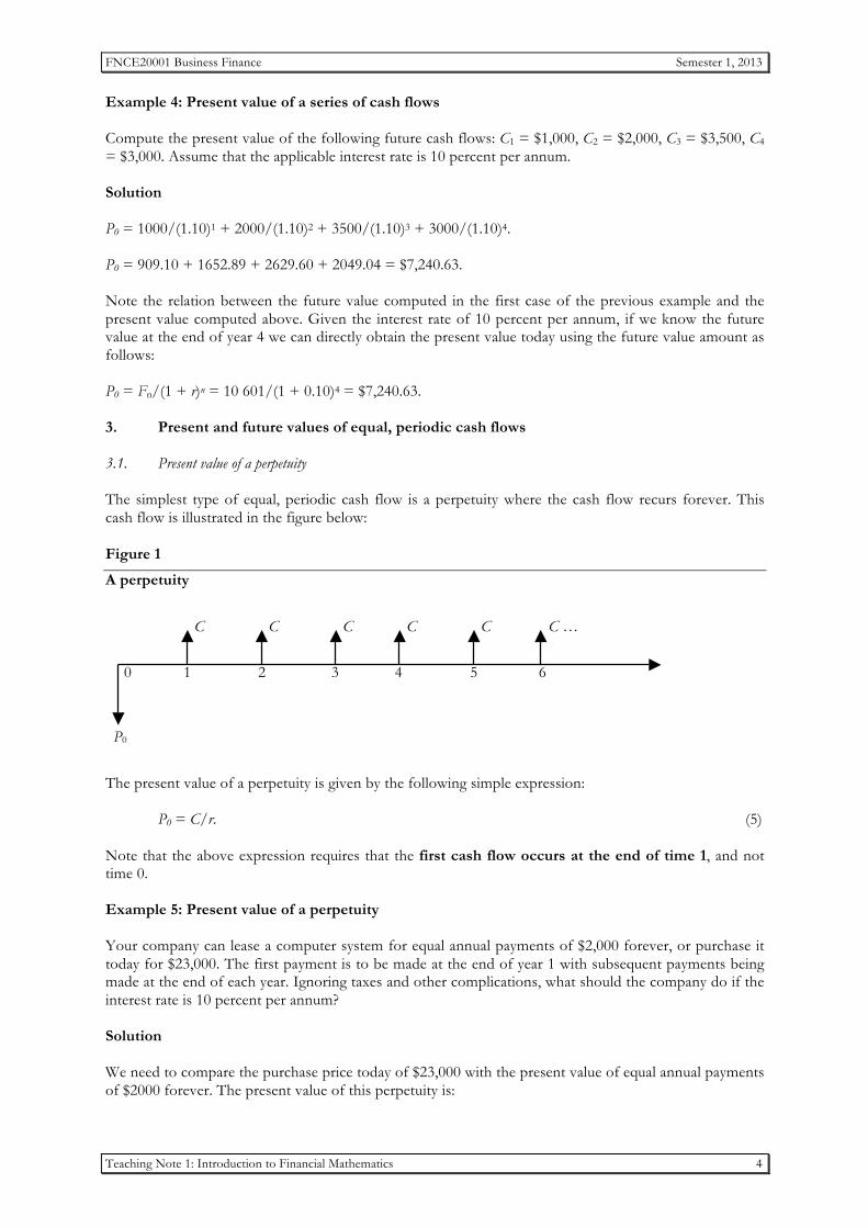
Example 4: Present value of a series of cash flows Compute the present value of the following future cash flows: C1 = $1,000, C2 = $2,000, C3 = $3,500, C4 = $3,000. Assume that the applicable interest rate is 10 percent per annum. Solution P0 = 1000/(1.10)1 + 2000/(1.10)2 + 3500/(1.10)3 + 3000/(1.10)4. P0 = 909.10 + 1652.89 + 2629.60 + 2049.04 = $7,240.63. Note the relation between the future value computed in the first case of the previous example and the present value computed above. Given the interest rate of 10 percent per annum, if we know the future value at the end of year 4 we can directly obtain the present value today using the future value amount as follows: P0 = Fn/(1 + r)n = 10 601/(1 + 0.10)4 = $7,240.63. 3. Present and future values of equal, periodic cash flows 3.1. Present value of a perpetuity The simplest type of equal, periodic cash flow is a perpetuity where the cash flow recurs forever. This cash flow is illustrated in the figure below: Figure 1

A perpetuity

The present value of a perpetuity is given by the following simple expression: P0 = C/r. (5) Note that the above expression requires that the first cash flow occurs at the end of time 1, and not time 0. Example 5: Present value of a perpetuity Your company can lease a computer system for equal annual payments of $2,000 forever, or purchase it today for $23,000. The first payment is to be made at the end of year 1 with subsequent payments being made at the end of each year. Ignoring taxes and other complications, what should the company do if the interest rate is 10 percent per annum? Solution We need to compare the purchase price today of $23,000 with the present value of equal annual payments of $2000 forever. The present value of this perpetuity is:

P0

C C C C C C …

0 1 2 3 4 5 6



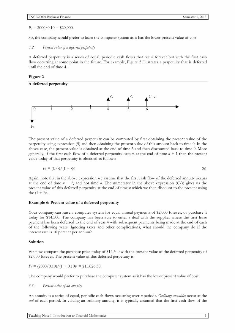
P0 = 2000/0.10 = $20,000. So, the company would prefer to lease the computer system as it has the lower present value of cost. 3.2. Present value of a deferred perpetuity A deferred perpetuity is a series of equal, periodic cash flows that recur forever but with the first cash flow occurring at some point in the future. For example, Figure 2 illustrates a perpetuity that is deferred until the end of time 4. Figure 2

A deferred perpetuity

The present value of a deferred perpetuity can be computed by first obtaining the present value of the perpetuity using expression (5) and then obtaining the present value of this amount back to time 0. In the above case, the present value is obtained at the end of time 3 and then discounted back to time 0. More generally, if the first cash flow of a deferred perpetuity occurs at the end of time n + 1 then the present value today of that perpetuity is obtained as follows: P0 = (C/r)/(1 + r)n. (6) Again, note that in the above expression we assume that the first cash flow of the deferred annuity occurs at the end of time n + 1, and not time n. The numerator in the above expression (C/r) gives us the present value of this deferred perpetuity at the end of time n which we then discount to the present using the (1 + r)n. Example 6: Present value of a deferred perpetuity Your company can lease a computer system for equal annual payments of $2,000 forever, or purchase it today for $14,500. The company has been able to enter a deal with the supplier where the first lease payment has been deferred to the end of year 4 with subsequent payments being made at the end of each of the following years. Ignoring taxes and other complications, what should the company do if the interest rate is 10 percent per annum? Solution We now compare the purchase price today of $14,500 with the present value of the deferred perpetuity of $2,000 forever. The present value of this deferred perpetuity is: P0 = (2000/0.10)/(1 + 0.10)3 = $15,026.30. The company would prefer to purchase the computer system as it has the lower present value of cost. 3.3. Present value of an annuity An annuity is a series of equal, periodic cash flows occurring over n periods. Ordinary annuities occur at the end of each period. In valuing an ordinary annuity, it is typically assumed that the first cash flow of the

P0

C C C …

0 1 2 3 4 5 6



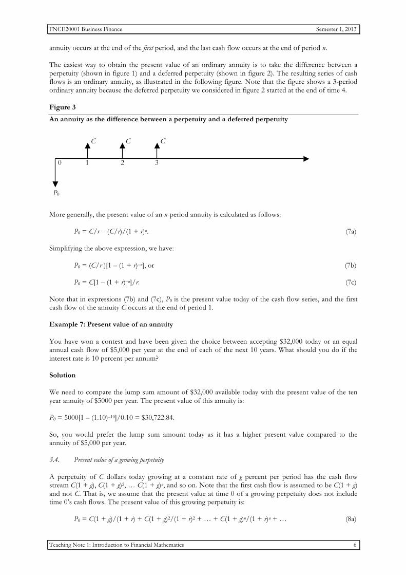
annuity occurs at the end of the first period, and the last cash flow occurs at the end of period n. The easiest way to obtain the present value of an ordinary annuity is to take the difference between a perpetuity (shown in figure 1) and a deferred perpetuity (shown in figure 2). The resulting series of cash flows is an ordinary annuity, as illustrated in the following figure. Note that the figure shows a 3-period ordinary annuity because the deferred perpetuity we considered in figure 2 started at the end of time 4. Figure 3

An annuity as the difference between a perpetuity and a deferred perpetuity

More generally, the present value of an n-period annuity is calculated as follows: P0 = C/r – (C/r)/(1 + r)n. (7a) Simplifying the above expression, we have: P0 = (C/r )[1 – (1 + r)–n], or (7b) P0 = C[1 – (1 + r)–n]/r. (7c) Note that in expressions (7b) and (7c), P0 is the present value today of the cash flow series, and the first cash flow of the annuity C occurs at the end of period 1. Example 7: Present value of an annuity You have won a contest and have been given the choice between accepting $32,000 today or an equal annual cash flow of $5,000 per year at the end of each of the next 10 years. What should you do if the interest rate is 10 percent per annum? Solution We need to compare the lump sum amount of $32,000 available today with the present value of the ten year annuity of $5000 per year. The present value of this annuity is: P0 = 5000[1 – (1.10)–10]/0.10 = $30,722.84. So, you would prefer the lump sum amount today as it has a higher present value compared to the annuity of $5,000 per year. 3.4. Present value of a growing perpetuity A perpetuity of C dollars today growing at a constant rate of g percent per period has the cash flow stream C(1 + g), C(1 + g)2, … C(1 + g)n, and so on. Note that the first cash flow is assumed to be C(1 + g) and not C. That is, we assume that the present value at time 0 of a growing perpetuity does not include time 0’s cash flows. The present value of this growing perpetuity is: P0 = C(1 + g)/(1 + r) + C(1 + g)2/(1 + r)2 + … + C(1 + g)n/(1 + r)n + … (8a)

P0

C C C

0 1 2 3



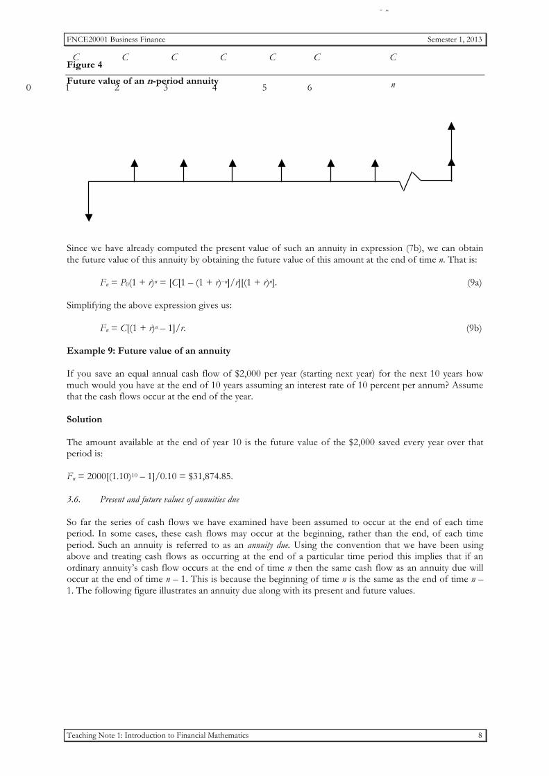
Multiplying expression (8a) through by (1 + g)/(1 + r), we have: P0(1 + g)/(1 + r) = C(1 + g)2/(1 + r)2 + … + C(1 + g)n+1/(1 + r)n+1+ … (8b) Subtracting expression (8b) from expression (8a) we get: P0 – P0(1 + g)/(1 + r) = C(1 + g)/(1 + r). (8c) Simplifying the above expression, we get: P0 = C(1 + g)/(1 + r)/[1 – (1 + g)/(1 + r)]. (8d) The above expression can be further simplified to give: P0 = C(1 + g)/(r – g). (8e) As noted above, expression (8e) assumes that the cash flow at time 1 is C(1 + g). In addition, for the above expression to be correctly defined we also need to assume that r > g. Example 8: Present value of a growing perpetuity Your company can lease a computer system for an annual lease payment of $1,800 next year with lease payments increasing at a constant annual rate of 2 percent forever, or purchase it today for $23,000. Assume an interest rate of 10 percent per annum. Ignoring taxes and other complications, what should the company do? How would your answer change if the first lease payment of $1,800 were due immediately (i.e., at the end of year 0) and then was to grow at a constant annual rate of 2 percent per annum forever? Assume end of the year cash flows. Solution A cash flow of $1,800 next year implies that C(1 + g) = $1,800. The present value of this growing perpetuity is: P0 = 1800/(0.10 – 0.02) = $22,500. So, the company would prefer to lease the computer system because the cost is lower in present value terms. If the first lease payment of $1,800 were due immediately then the present value of the cost of leasing is: New present value of cost of leasing, P0 = 1800 + 1800(1.02)/(0.10 – 0.02) = $24,750. The company would now prefer to purchase the computer system for $23,000 rather than leasing it. 3.5. Future value of an annuity The future value at the end of period n of an n-period annuity is the sum of the future values of each of these n cash flows. The cash flows are shown in the following figure.



Figure 4

Future value of an n-period annuity

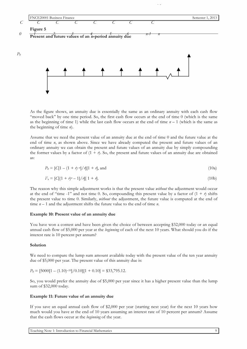
Since we have already computed the present value of such an annuity in expression (7b), we can obtain the future value of this annuity by obtaining the future value of this amount at the end of time n. That is: Fn = P0(1 + r)n = [C[1 – (1 + r)–n]/r][(1 + r)n]. (9a) Simplifying the above expression gives us: Fn = C[(1 + r)n – 1]/r. (9b) Example 9: Future value of an annuity If you save an equal annual cash flow of $2,000 per year (starting next year) for the next 10 years how much would you have at the end of 10 years assuming an interest rate of 10 percent per annum? Assume that the cash flows occur at the end of the year. Solution The amount available at the end of year 10 is the future value of the $2,000 saved every year over that period is: Fn = 2000[(1.10)10 – 1]/0.10 = $31,874.85. 3.6. Present and future values of annuities due So far the series of cash flows we have examined have been assumed to occur at the end of each time period. In some cases, these cash flows may occur at the beginning, rather than the end, of each time period. Such an annuity is referred to as an annuity due. Using the convention that we have been using above and treating cash flows as occurring at the end of a particular time period this implies that if an ordinary annuity’s cash flow occurs at the end of time n then the same cash flow as an annuity due will occur at the end of time n – 1. This is because the beginning of time n is the same as the end of time n – 1. The following figure illustrates an annuity due along with its present and future values.

Fn

C C C C C C

0 1 2 n 3 4 5 6

C



Figure 5

Present and future values of an n-period annuity due

As the figure shows, an annuity due is essentially the same as an ordinary annuity with each cash flow “moved back” by one time period. So, the first cash flow occurs at the end of time 0 (which is the same as the beginning of time 1) while the last cash flow occurs at the end of time n – 1 (which is the same as the beginning of time n). Assume that we need the present value of an annuity due at the end of time 0 and the future value at the end of time n, as shown above. Since we have already computed the present and future values of an ordinary annuity we can obtain the present and future values of an annuity due by simply compounding the former values by a factor of (1 + r). So, the present and future values of an annuity due are obtained as: P0 = [C[1 – (1 + r)–n]/r][1 + r], and (10a) Fn = [C[(1 + r)n – 1]/r][ 1 + r]. (10b) The reason why this simple adjustment works is that the present value without the adjustment would occur at the end of “time -1” and not time 0. So, compounding this present value by a factor of (1 + r) shifts the present value to time 0. Similarly, without the adjustment, the future value is computed at the end of time n – 1 and the adjustment shifts the future value to the end of time n. Example 10: Present value of an annuity due You have won a contest and have been given the choice of between accepting $32,000 today or an equal annual cash flow of $5,000 per year at the beginning of each of the next 10 years. What should you do if the interest rate is 10 percent per annum? Solution We need to compare the lump sum amount available today with the present value of the ten year annuity due of $5,000 per year. The present value of this annuity due is: P0 = [5000[1 – (1.10)–10]/0.10][1 + 0.10] = $33,795.12. So, you would prefer the annuity due of $5,000 per year since it has a higher present value than the lump sum of $32,000 today. Example 11: Future value of an annuity due If you save an equal annual cash flow of $2,000 per year (starting next year) for the next 10 years how much would you have at the end of 10 years assuming an interest rate of 10 percent per annum? Assume that the cash flows occur at the beginning of the year.

P0

Fn

C C C C C C

0 1 2 n

C

3 4 5 6

C

n-1



Solution The amount available at the end of year 10 is the future value of the annuity due of $2,000 every year over that period is:

Fn = [2000[(1.10)10 – 1]/0.10][1 + 0.10] = $35,062.33. Practice Problem 1 You have just won a lottery and have been offered the following alternative ways of receiving the prize money. Assume that each alternative is risk free and the interest rate is 8 percent per annum. a) $110,000 immediately. b) $140,000 at the end of year 3. c) $28,000 at the end of each of the next 5 years. d) $9,000 at the end of each year in perpetuity. e) $6,500 at the end of the first year growing at a rate of 2 percent in perpetuity. Assuming end of the year cash flows, which is the best way to receive the prize money? Practice Problem 2 Assume that the interest rate is 10 percent per annum and that all cash flows occur at the end of each year. Round off your final answers to the nearest dollar. a) Suppose you decide to invest $50,000 today. Compute the total value of your investment at the

end of 10 years. b) Your friend also decides to invest $50,000 but plans to do so in installments. Specifically, she will

invest $5,000 now, $10,000 at the end of year 1, $15,000 at the end of year 2, and $20,000 at the end of year 3. Compute the total value of her investment at the end of 10 years.

c) Another friend of yours also decides to invest $50,000 but to defer the investment until the end

of year 3. Compute the total value of his investment at the end of 10 years. d) Now assume that you and your friends have an investment time horizon of 10 years. What

additional amount would your friends have to invest today so that, at the end of year 10, the total value of their respective investments is the same as the total value of your investment?

e) Suppose that instead of investing the additional amounts today in part (d) your friends decide to

invest funds in equal annual amounts over the ten-year period. Compute the amounts that the two friends would now need to invest.

f) Now suppose that you and your friends decide to invest funds in equal annual amounts over the

ten-year period so each of you has the same total value at the end of ten years as computed in part (a). What would this equal annual amount be?

g) How does your answer in part (f) change if the equal annual amounts were invested at the

beginning of each year rather than at the end of each year as assumed above?



4. Some applications of financial mathematics 4.1. Valuing home mortgages In a standard, fixed-rate mortgage, a lump sum cash flow (i.e., the loan amount) is exchanged for equal, periodic payments over the duration of the mortgage. The payments are typically made on a monthly basis where each payment equals the sum of the interest payment and principal repayment. Computing the value of such a mortgage at any point over the loan’s time horizon is a specific application of the present value of an annuity. Calculating the periodic loan payments Assume P0 is borrowed today at an interest rate of r percent per period to be repaid in n equal payments of C dollars per period. Assuming that the periodic payment is made at the end of each period we have an n-period ordinary annuity. The amount borrowed today is the present value of this annuity as shown in expression (7c): P0 = C[1 – (1 + r)–n]/r. (7c) Re-arranging the above expression we can obtain the periodic payment as: C = r × P0/[1 – (1 + r)–n]. (7d) Example 12: Valuing a home mortgage A 25-year home loan for $100,000 has a monthly interest rate of 1 percent and payments are to be made at the end of each month. Compute the monthly payment on this loan. Compute the principal balance remaining at the end of the (a) first and (b) fifth year of the loan. Solution In this case, N = 25 × 12 = 300 months. Using expression (7d) we can obtain the monthly payment as: Monthly payment, C = 0.01(100000)/(1 – 1.01–300) = $1,053.22. The process of discounting the monthly payment essentially “strips off” the interest component from each month’s payment. We can therefore use expression (7c) to calculate the principal balance remaining on the loan at the end of any time period. The principal balance remaining at the end of the first year of the loan (i.e., after 12 months) is the present value of the remaining 288 (= 300 – 12) monthly payments, which is: P12 = 1053.22[1 – (1.01)–288]/0.01 = $99,324.59. Similarly, the principal balance remaining at the end of the fifth year of the loan (i.e., after 60 months) is the present value of the remaining 240 (= 300 – 60) monthly payments, which is: P60 = 1053.22[1 – (1.01)–240]/0.01 = $95,652.83. Obtaining the loan amortization schedule A loan amortization schedule shows the total payments on a loan and breaks up this amount into the interest paid in a particular period, the principal balance repaid in that period and the principal balance outstanding at the end of that period. The interest paid in any period is calculated as the per-period interest rate multiplied by the principal balance at the start of that period which is equal to the principal balance at



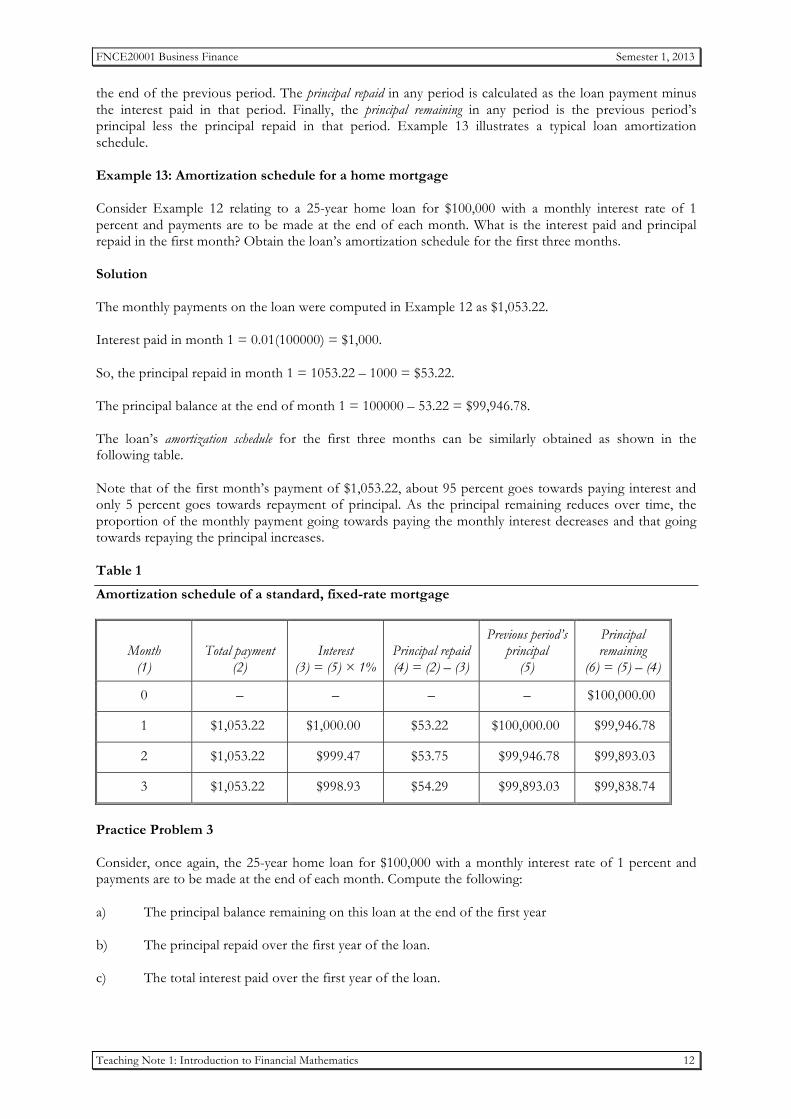
the end of the previous period. The principal repaid in any period is calculated as the loan payment minus the interest paid in that period. Finally, the principal remaining in any period is the previous period’s principal less the principal repaid in that period. Example 13 illustrates a typical loan amortization schedule. Example 13: Amortization schedule for a home mortgage Consider Example 12 relating to a 25-year home loan for $100,000 with a monthly interest rate of 1 percent and payments are to be made at the end of each month. What is the interest paid and principal repaid in the first month? Obtain the loan’s amortization schedule for the first three months. Solution The monthly payments on the loan were computed in Example 12 as $1,053.22. Interest paid in month 1 = 0.01(100000) = $1,000. So, the principal repaid in month 1 = 1053.22 – 1000 = $53.22. The principal balance at the end of month 1 = 100000 – 53.22 = $99,946.78. The loan’s amortization schedule for the first three months can be similarly obtained as shown in the following table. Note that of the first month’s payment of $1,053.22, about 95 percent goes towards paying interest and only 5 percent goes towards repayment of principal. As the principal remaining reduces over time, the proportion of the monthly payment going towards paying the monthly interest decreases and that going towards repaying the principal increases. Table 1

Amortization schedule of a standard, fixed-rate mortgage

Month (1)

Total payment (2)

Interest (3) = (5) × 1%

Principal repaid (4) = (2) – (3)

Previous period’s principal

(5)

Principal remaining

(6) = (5) – (4)

0 – – – – $100,000.00

1 $1,053.22 $1,000.00 $53.22 $100,000.00 $99,946.78

2 $1,053.22 $999.47 $53.75 $99,946.78 $99,893.03

3 $1,053.22 $998.93 $54.29 $99,893.03 $99,838.74

Practice Problem 3 Consider, once again, the 25-year home loan for $100,000 with a monthly interest rate of 1 percent and payments are to be made at the end of each month. Compute the following: a) The principal balance remaining on this loan at the end of the first year b) The principal repaid over the first year of the loan. c) The total interest paid over the first year of the loan.



4.2. Valuing debt securities The basic valuation process for financial securities, including debt and equity securities, involves obtaining the present value of the future cash flows that the security is expected to generate. Thus, the valuation process essentially involves applying the concepts discussed above. In general, debt securities are securities where the issuer borrows funds from investors with a contractual obligation to make regular interest payments to these investors as well as repay the funds borrowed when the contract matures in the future. The simplest type of debt security is one that pays a fixed amount (the face or maturity value) at some time in the future and no other cash flow over its life. Examples of this type of security are Treasury bills and bank bills which mature in less than a year and zero coupon bonds which typically have maturity dates well into the future. Example 14: Valuing discount securities Consider a Treasury bill with a face (or maturity) value of $100,000 and which matures in 180 days. Assuming that the market yield on this security is 6% p.a. what is its price today? Solution Since the security matures in 180 days we first need to compute the appropriate market yield over the security’s life. As there are 365 days in the year, the market yield appropriate over the 180-day period is: 180-day market yield = (n/365) × r = (180/365) × 0.06 = 0.02959 or 2.959%. The price can then be computed as the present value of the face value, which is: Price = 100000/[1 + 0.02959] = $97,126.13. Example 15: Valuing a zero coupon bond A zero coupon bond matures in 5 years and has a face value of $1,000. Compute the price of the bond today if the market yield on the bond is 8% p.a. Solution The price of the bond today is the present value of the face value which investors will receive at maturity 5 years from now. That is: P0 = 1000/(1 + 0.08)5 = $680.58. Valuing coupon paying debt securities is a little more complex because it involves obtaining the present value of the face value at maturity and the promised periodic coupon (or interest) payments, which are stated as a percentage of the face value. The coupon payments are typically made on a semi-annual basis but their valuation can be approximated quite well assuming annual coupon payments. So, the value of such securities can be obtained as the sum of the present value of the face value and the interest annuity, as shown in Example 16. Example 16: Valuing a coupon paying bond Consider a bond which pays a coupon of 10 percent on a semi-annual basis with 5 years to maturity and a face value of $1,000. If the bond has a market yield of 8 percent what price should it be selling for today? What would the price of this security be if the coupons were paid on an annual basis?



Solution The price of the security is equal to the present value of the annuity of coupon payments on the face value of $1000 and the face value paid at the end of year 5. As the coupons are paid semi-annually we have: Semi-annual coupon payments = 0.10/2 × 1000 = $50. There are 10 (= 5 × 2) coupon payments over the life of the security. So the appropriate semi-annual market yield is 4% (= 8/2). The price today should be: P0 = 50[(1 – (1 + 0.04)–10)/0.04] + 1000/(1 + 0.04)10. P0 = 405.54 + 675.56 = $1,081.10. Assuming that the coupons are paid on an annual basis gives the following price for the bond: P0 = 100[(1 – (1 + 0.08)–5)/0.08] + 1000/(1 + 0.08)5. P0 = 399.27 + 680.58 = $1,079.85. 4.3. Valuing equity securities The two most common types of equity securities are preference shares and ordinary shares. Unlike debt securities, there are no obligations for payments to be made to such shareholders. Dividends to preference shareholders are typically based on the face value of the shares on issue and are valued as the present value of a perpetuity, as shown in Example 17. Example 17: Valuing preference shares ACB Ltd has 8% $100 preference shares on issue and on which investors require a return of 10 percent per annum. At what price should these shares be selling for today? Solution The price of the preference shares are obtained as the present value of the expected perpetual dividend stream. The dividend stream from the preference shares is: D = 0.08 × 100 = $8.00. The price of the preference shares is: P0 = D/r = (0.08 × 100)/0.10 = $80.00. Dividends to ordinary shareholders need not follow any particular pattern although companies with a policy of paying regular dividends generally like to maintain either a constant dividend payout or with dividends growing over time. Thus, ordinary shares can often be valued as the present value of a perpetual stream of expected future dividends or a growing perpetuity over time, as shown in Example 18. Example 18: Valuing ordinary shares You are valuing the ordinary shares of four companies which are expected to pay the following dividends over time: !! BCA Ltd is expected to pay a dividend of $1.00 per year forever.



!! DCA Ltd is expected to pay a dividend of $1.00 next year with this amount expected to grow at a constant rate of 5% per annum forever.

!! FCA Ltd is not expected to pay a dividend for the next 3 years and then pay a dividend of $1.00 per

year forever. !! HCA Ltd is not expected to pay a dividend for the next 3 years and then pay a dividend of $1.00 per

year which is expected to grow at a constant rate of 5% per annum forever. What are your price estimates for each company if investors require a return of 10 percent per annum on all these companies? Solution BCA’s shares can be valued as the present value of a perpetuity. That is: BCA’s price = D/r = 1.00/0.10 = $10.00. DCA’s shares can be valued as the present value of a growing perpetuity. That is: DCA’s price = D1/(r – g)= 1.00/(0.10 – 0.05) = $20.00. FCA’s shares can be valued as the present value of a deferred perpetuity. That is: FCA’s price = [D4/r ]/(1 + r)3 = [1.00/0.10]/(1 + 0.10)3 = $7.51. HCA’s shares can be valued as the present value of a deferred perpetuity that grows at a constant rate. That is: HCA’s price = [D4/(r – g) ]/(1 + r)3 = [1.00/(0.10 – 0.05)]/(1 + 0.10)3 = $15.03. 5. Effective interest rates The above discussion assumes that interest is paid or received annually. However, this is often not the case. In the mortgage example, interest is paid on the monthly principal balance outstanding. Although the monthly interest rate in our mortgage example was 1 percent, the effective annual interest rate is not 12 percent because interest on the loan is computed (i.e., compounded) more frequently than once a year. The effective annual interest rate will differ from the nominal (or quoted) annual interest rate as long as interest is computed more often than once a year. If the stated annual interest rate is r percent and interest is computed m times a year, the per-period interest rate is r/m percent and the effective annual interest rate is calculated as: re = (1 + r/m)m – 1. (11) The above expression means that if we invest $1 at the quoted annual interest rate of r percent, but where interest is compounded m times during the year, our initial $1 investment will amount to $(1 + r/m)m by the end of the year. The effective annual interest rate would be as in expression (11). Note that if interest is calculated once a year (m = 1), then re = r. Continuous compounding The compounding interval becomes continuous as m approaches infinity; the expression (1 + r/m)m approaches e r, where e is the exponential constant taking the value 2.718281. With continuous compounding, the effective interest rate is computed as: re = e r – 1. (12)



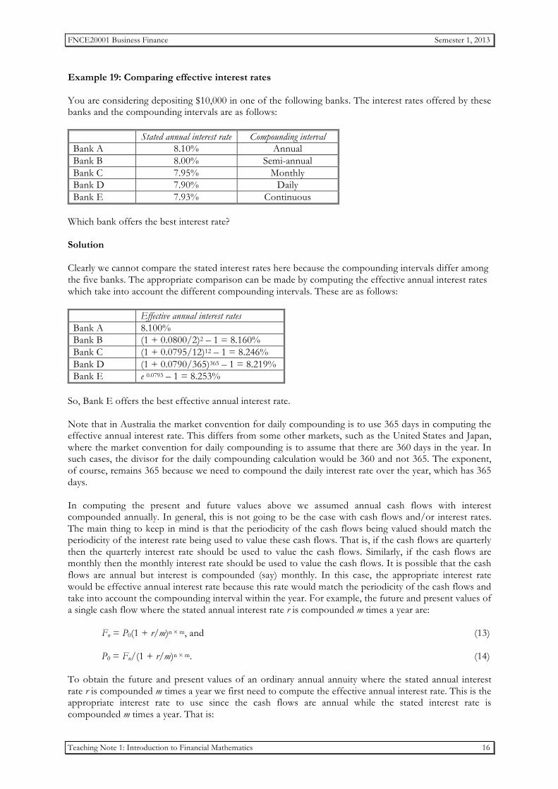
Example 19: Comparing effective interest rates You are considering depositing $10,000 in one of the following banks. The interest rates offered by these banks and the compounding intervals are as follows:

Stated annual interest rate Compounding interval Bank A 8.10% Annual Bank B 8.00% Semi-annual Bank C 7.95% Monthly Bank D 7.90% Daily Bank E 7.93% Continuous

Which bank offers the best interest rate? Solution Clearly we cannot compare the stated interest rates here because the compounding intervals differ among the five banks. The appropriate comparison can be made by computing the effective annual interest rates which take into account the different compounding intervals. These are as follows:

Effective annual interest rates Bank A 8.100% Bank B (1 + 0.0800/2)2 – 1 = 8.160% Bank C (1 + 0.0795/12)12 – 1 = 8.246% Bank D (1 + 0.0790/365)365 – 1 = 8.219% Bank E e 0.0793 – 1 = 8.253%

So, Bank E offers the best effective annual interest rate. Note that in Australia the market convention for daily compounding is to use 365 days in computing the effective annual interest rate. This differs from some other markets, such as the United States and Japan, where the market convention for daily compounding is to assume that there are 360 days in the year. In such cases, the divisor for the daily compounding calculation would be 360 and not 365. The exponent, of course, remains 365 because we need to compound the daily interest rate over the year, which has 365 days. In computing the present and future values above we assumed annual cash flows with interest compounded annually. In general, this is not going to be the case with cash flows and/or interest rates. The main thing to keep in mind is that the periodicity of the cash flows being valued should match the periodicity of the interest rate being used to value these cash flows. That is, if the cash flows are quarterly then the quarterly interest rate should be used to value the cash flows. Similarly, if the cash flows are monthly then the monthly interest rate should be used to value the cash flows. It is possible that the cash flows are annual but interest is compounded (say) monthly. In this case, the appropriate interest rate would be effective annual interest rate because this rate would match the periodicity of the cash flows and take into account the compounding interval within the year. For example, the future and present values of a single cash flow where the stated annual interest rate r is compounded m times a year are: Fn = P0(1 + r/m)n × m, and (13) P0 = Fn/(1 + r/m)n × m. (14) To obtain the future and present values of an ordinary annual annuity where the stated annual interest rate r is compounded m times a year we first need to compute the effective annual interest rate. This is the appropriate interest rate to use since the cash flows are annual while the stated interest rate is compounded m times a year. That is:



re = (1 + r/m)m – 1. The future and present values of an ordinary annual annuity over n years can then be computed as:

(1 ) 1n

en

e

rF Ar

+ −= × , and (15)

01 (1 ) ne

e

rP Ar

−− += × . (16)

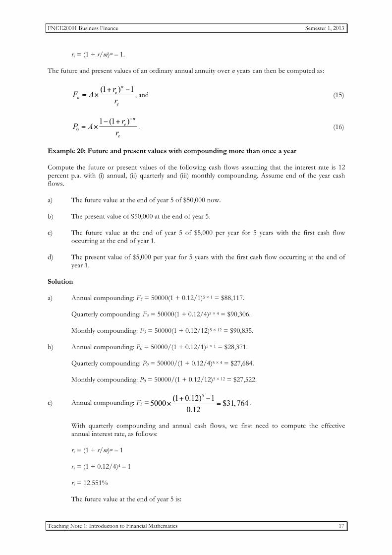
Example 20: Future and present values with compounding more than once a year Compute the future or present values of the following cash flows assuming that the interest rate is 12 percent p.a. with (i) annual, (ii) quarterly and (iii) monthly compounding. Assume end of the year cash flows. a) The future value at the end of year 5 of $50,000 now. b) The present value of $50,000 at the end of year 5. c) The future value at the end of year 5 of $5,000 per year for 5 years with the first cash flow

occurring at the end of year 1. d) The present value of $5,000 per year for 5 years with the first cash flow occurring at the end of

year 1. Solution a) Annual compounding: F5 = 50000(1 + 0.12/1)5 × 1 = $88,117. Quarterly compounding: F5 = 50000(1 + 0.12/4)5 × 4 = $90,306. Monthly compounding: F5 = 50000(1 + 0.12/12)5 × 12 = $90,835. b) Annual compounding: P0 = 50000/(1 + 0.12/1)5 × 1 = $28,371. Quarterly compounding: P0 = 50000/(1 + 0.12/4)5 × 4 = $27,684. Monthly compounding: P0 = 50000/(1 + 0.12/12)5 × 12 = $27,522.

c) Annual compounding: F5 =5(1 0.12) 15000 $31,764

0.12+ −

× = .

With quarterly compounding and annual cash flows, we first need to compute the effective

annual interest rate, as follows: re = (1 + r/m)m – 1 re = (1 + 0.12/4)4 – 1 re = 12.551% The future value at the end of year 5 is:



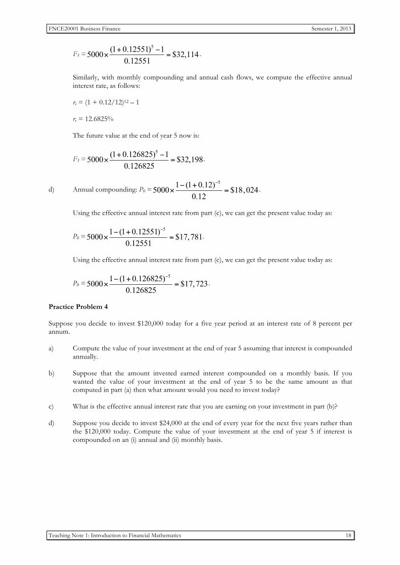
F5 =5(1 0.12551) 15000 $32,114

0.12551+ −

× = .

Similarly, with monthly compounding and annual cash flows, we compute the effective annual

interest rate, as follows: re = (1 + 0.12/12)12 – 1 re = 12.6825% The future value at the end of year 5 now is:

F5 =5(1 0.126825) 15000 $32,198

0.126825+ −

× = .

d) Annual compounding: P0 =51 (1 0.12)5000 $18,024

0.12

−− +× = .

Using the effective annual interest rate from part (c), we can get the present value today as:

P0 =51 (1 0.12551)5000 $17,781

0.12551

−− +× = .

Using the effective annual interest rate from part (c), we can get the present value today as:

P0 =51 (1 0.126825)5000 $17,723

0.126825

−− +× = .

Practice Problem 4 Suppose you decide to invest $120,000 today for a five year period at an interest rate of 8 percent per annum. a) Compute the value of your investment at the end of year 5 assuming that interest is compounded

annually. b) Suppose that the amount invested earned interest compounded on a monthly basis. If you

wanted the value of your investment at the end of year 5 to be the same amount as that computed in part (a) then what amount would you need to invest today?

c) What is the effective annual interest rate that you are earning on your investment in part (b)? d) Suppose you decide to invest $24,000 at the end of every year for the next five years rather than

the $120,000 today. Compute the value of your investment at the end of year 5 if interest is compounded on an (i) annual and (ii) monthly basis.



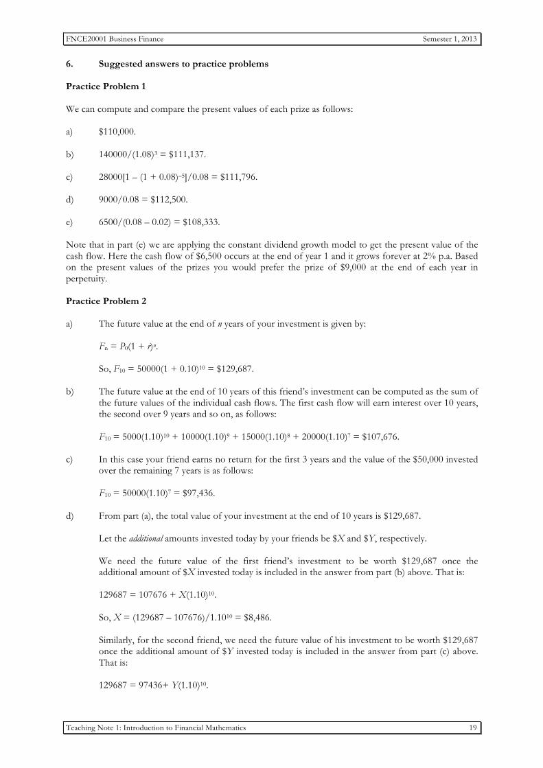
6. Suggested answers to practice problems Practice Problem 1 We can compute and compare the present values of each prize as follows: a) $110,000. b) 140000/(1.08)3 = $111,137. c) 28000[1 – (1 + 0.08)–5]/0.08 = $111,796. d) 9000/0.08 = $112,500. e) 6500/(0.08 – 0.02) = $108,333. Note that in part (e) we are applying the constant dividend growth model to get the present value of the cash flow. Here the cash flow of $6,500 occurs at the end of year 1 and it grows forever at 2% p.a. Based on the present values of the prizes you would prefer the prize of $9,000 at the end of each year in perpetuity. Practice Problem 2 a) The future value at the end of n years of your investment is given by:

Fn = P0(1 + r)n.

So, F10 = 50000(1 + 0.10)10 = $129,687. b) The future value at the end of 10 years of this friend’s investment can be computed as the sum of

the future values of the individual cash flows. The first cash flow will earn interest over 10 years, the second over 9 years and so on, as follows:

F10 = 5000(1.10)10 + 10000(1.10)9 + 15000(1.10)8 + 20000(1.10)7 = $107,676.

c) In this case your friend earns no return for the first 3 years and the value of the $50,000 invested

over the remaining 7 years is as follows: F10 = 50000(1.10)7 = $97,436. d) From part (a), the total value of your investment at the end of 10 years is $129,687.

Let the additional amounts invested today by your friends be $X and $Y, respectively. We need the future value of the first friend’s investment to be worth $129,687 once the additional amount of $X invested today is included in the answer from part (b) above. That is: 129687 = 107676 + X(1.10)10. So, X = (129687 – 107676)/1.1010 = $8,486. Similarly, for the second friend, we need the future value of his investment to be worth $129,687 once the additional amount of $Y invested today is included in the answer from part (c) above. That is: 129687 = 97436+ Y(1.10)10.



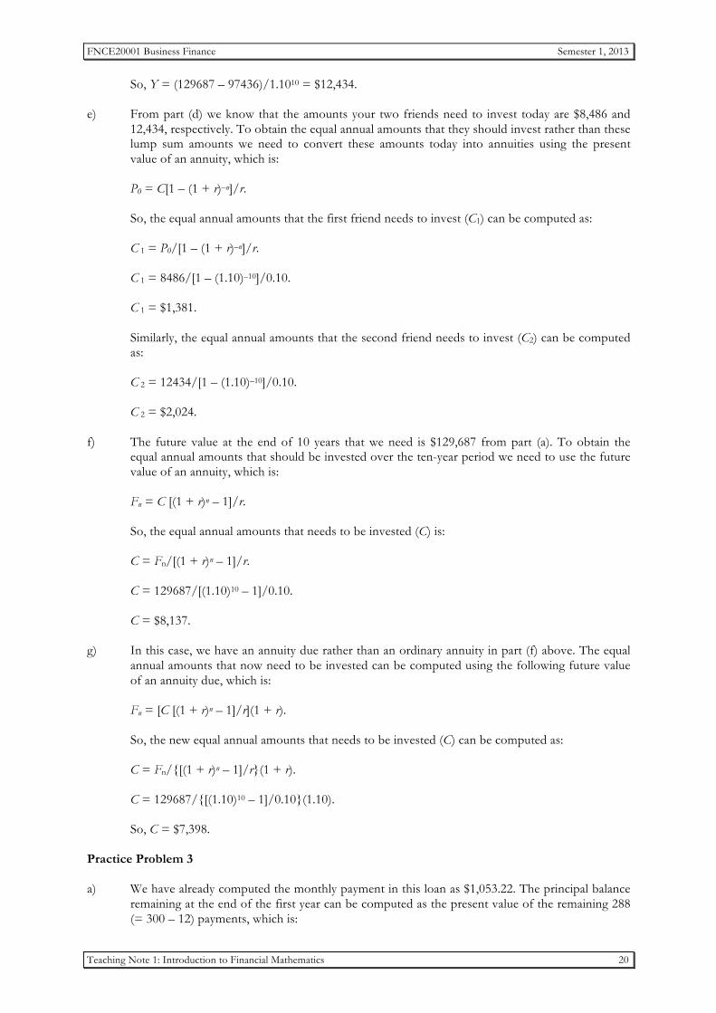
So, Y = (129687 – 97436)/1.1010 = $12,434. e) From part (d) we know that the amounts your two friends need to invest today are $8,486 and

12,434, respectively. To obtain the equal annual amounts that they should invest rather than these lump sum amounts we need to convert these amounts today into annuities using the present value of an annuity, which is:

P0 = C[1 – (1 + r)–n]/r. So, the equal annual amounts that the first friend needs to invest (C1) can be computed as: C 1 = P0/[1 – (1 + r)–n]/r. C 1 = 8486/[1 – (1.10)–10]/0.10. C 1 = $1,381. Similarly, the equal annual amounts that the second friend needs to invest (C2) can be computed

as: C 2 = 12434/[1 – (1.10)–10]/0.10. C 2 = $2,024. f) The future value at the end of 10 years that we need is $129,687 from part (a). To obtain the

equal annual amounts that should be invested over the ten-year period we need to use the future value of an annuity, which is:

Fn = C [(1 + r)n – 1]/r. So, the equal annual amounts that needs to be invested (C) is:

C = Fn/[(1 + r)n – 1]/r.

C = 129687/[(1.10)10 – 1]/0.10.

C = $8,137. g) In this case, we have an annuity due rather than an ordinary annuity in part (f) above. The equal

annual amounts that now need to be invested can be computed using the following future value of an annuity due, which is:

Fn = [C [(1 + r)n – 1]/r](1 + r). So, the new equal annual amounts that needs to be invested (C) can be computed as:

C = Fn/{[(1 + r)n – 1]/r}(1 + r).

C = 129687/{[(1.10)10 – 1]/0.10}(1.10).

So, C = $7,398. Practice Problem 3 a) We have already computed the monthly payment in this loan as $1,053.22. The principal balance

remaining at the end of the first year can be computed as the present value of the remaining 288 (= 300 – 12) payments, which is:



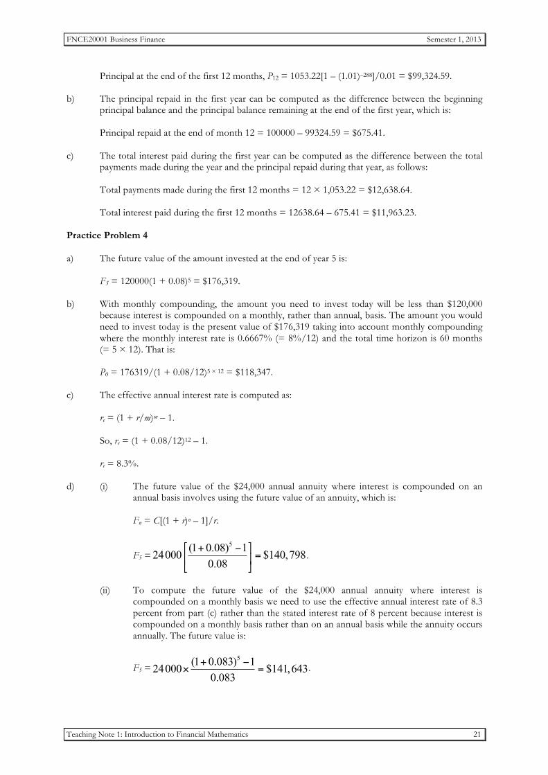
Principal at the end of the first 12 months, P12 = 1053.22[1 – (1.01)–288]/0.01 = $99,324.59.

b) The principal repaid in the first year can be computed as the difference between the beginning

principal balance and the principal balance remaining at the end of the first year, which is:

Principal repaid at the end of month 12 = 100000 – 99324.59 = $675.41. c) The total interest paid during the first year can be computed as the difference between the total

payments made during the year and the principal repaid during that year, as follows:

Total payments made during the first 12 months = 12 × 1,053.22 = $12,638.64.

Total interest paid during the first 12 months = 12638.64 – 675.41 = $11,963.23. Practice Problem 4 a) The future value of the amount invested at the end of year 5 is: F5 = 120000(1 + 0.08)5 = $176,319. b) With monthly compounding, the amount you need to invest today will be less than $120,000

because interest is compounded on a monthly, rather than annual, basis. The amount you would need to invest today is the present value of $176,319 taking into account monthly compounding where the monthly interest rate is 0.6667% (= 8%/12) and the total time horizon is 60 months (= 5 × 12). That is:

P0 = 176319/(1 + 0.08/12)5 × 12 = $118,347. c) The effective annual interest rate is computed as: re = (1 + r/m)m – 1. So, re = (1 + 0.08/12)12 – 1. re = 8.3%. d) (i) The future value of the $24,000 annual annuity where interest is compounded on an

annual basis involves using the future value of an annuity, which is:

Fn = C[(1 + r)n – 1]/r.

F5 =5(1 0.08) 124000 $140,798

0.08! "+ −

=$ %& '

.

(ii) To compute the future value of the $24,000 annual annuity where interest is

compounded on a monthly basis we need to use the effective annual interest rate of 8.3 percent from part (c) rather than the stated interest rate of 8 percent because interest is compounded on a monthly basis rather than on an annual basis while the annuity occurs annually. The future value is:

F5 =5(1 0.083) 124000 $141,643

0.083+ −

× = .



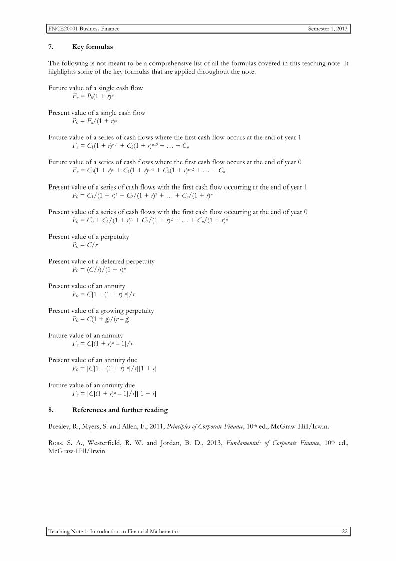
7. Key formulas The following is not meant to be a comprehensive list of all the formulas covered in this teaching note. It highlights some of the key formulas that are applied throughout the note. Future value of a single cash flow Fn = P0(1 + r)n Present value of a single cash flow P0 = Fn/(1 + r)n Future value of a series of cash flows where the first cash flow occurs at the end of year 1 Fn = C1(1 + r)n-1 + C2(1 + r)n-2 + … + Cn Future value of a series of cash flows where the first cash flow occurs at the end of year 0

Fn = C0(1 + r)n + C1(1 + r)n-1 + C2(1 + r)n-2 + … + Cn

Present value of a series of cash flows with the first cash flow occurring at the end of year 1 P0 = C1/(1 + r)1 + C2/(1 + r)2 + … + Cn/(1 + r)n Present value of a series of cash flows with the first cash flow occurring at the end of year 0

P0 = C0 + C1/(1 + r)1 + C2/(1 + r)2 + … + Cn/(1 + r)n Present value of a perpetuity P0 = C/r Present value of a deferred perpetuity P0 = (C/r)/(1 + r)n Present value of an annuity P0 = C[1 – (1 + r)–n]/r Present value of a growing perpetuity P0 = C(1 + g)/(r – g) Future value of an annuity Fn = C[(1 + r)n – 1]/r Present value of an annuity due P0 = [C[1 – (1 + r)–n]/r][1 + r] Future value of an annuity due Fn = [C[(1 + r)n – 1]/r][ 1 + r] 8. References and further reading Brealey, R., Myers, S. and Allen, F., 2011, Principles of Corporate Finance, 10th ed., McGraw-Hill/Irwin. Ross, S. A., Westerfield, R. W. and Jordan, B. D., 2013, Fundamentals of Corporate Finance, 10th ed., McGraw-Hill/Irwin.

Documents

Teaching Note 1 - Financial Math