Teaching New Keynesian Open Economy Macroeconomics at the

Intermediate Level

Peter Bofinger,

Professor of Economics, University of Wuerzburg and CEPR

Eric Mayer, Research and Teaching Assistant, University of Wuerzburg

Timo Wollmershäuser, Economist, Ifo Institute for Economic Research, Munich

Mailing Address: Timo Wollmershaeuser Ifo Institute for Economic Research Department of Business Cycle Analyses and Financial Markets Poschingerstrasse 5 81679 München Germany Email: wollmershaeuser@ifo.de Phone: +49 (89) 9224-1406 Fax: +49 (89) 9224-1462

---Abstract---

For the open economy the workhorse model in intermediate textbooks still is the Mundell-Fleming model, which basically extends the IS-LM model to open economy problems. The purpose of this paper is to present a simple New Keynesian model of the open economy, that introduces open economy considerations into the closed economy consensus version and that still allows for a simple and comprehensible analytical and graphical treatment. Above all, our model provides an efficient tool kit for the discussion of the costs and benefits of fixed and flexible exchange rates, which also was at the core of the Mundell-Fleming model. JEL classification: A 20, E 10, E 50, F 41 Keywords: open economy, inflation targeting, monetary policy rules, New Keynesian macroeconomics

The authors would like to thank Carol Osler, Stefan Reitz and Michael Woodford for extremely helpful and valuable comments.

Teaching New Keynesian Open Economy Macroeconomics at the

Intermediate Level

---Abstract---

For the open economy the workhorse model in intermediate textbooks still is the Mundell-Fleming model, which basically extends the IS-LM model to open economy problems. The purpose of this paper is to present a simple New Keynesian model of the open economy, that introduces open economy considerations into the closed economy consensus version and that still allows for a simple and comprehensible analytical and graphical treatment. Above all, our model provides an efficient tool kit for the discussion of the costs and benefits of fixed and flexible exchange rates, which also was at the core of the Mundell-Fleming model. JEL classification: A 20, E 10, E 50, F 41 Keywords: open economy, inflation targeting, monetary policy rules, New Keynesian macroeconomics

The authors would like to thank Carol Osler, Stefan Reitz and Michael Woodford for extremely helpful and valuable comments.

1

1 Introduction

In recent years a range of papers have been published trying to present an alternative

intermediate macroeconomic textbook model to the outdated IS-LM-AS-AD model. Among

them the most influential have been the IS-MP (monetary policy)-IA (inflation adjustment)

model by Romer (2000), the inflation targeting model by Walsh (2002), the AD (aggregate

demand)-PA (price adjustment) model by Weerapana (2003), the IS-PC (Phillips curve)-MR

(monetary policy rule) model by Carlin and Soskice (2004), and the BMW model by Bofinger,

Mayer and Wollmershäuser (2005). Similar to the class of dynamic New Keynesian macro

models popularised by Clarida, Gali and Gertler (1999) the main building blocks in all models

are an IS equation, that links the output gap to the real interest rate, a Phillips curve that relates

the inflation rate to the output gap, and a monetary policy rule that is evaluated in terms of or

derived from a social loss function. While the IS equation has survived the New Keynesian

revolution (even though it is nowadays derived from solid micro-foundations), the major

innovations with respect to the IS-LM-AS-AD model are

- that monetary policy is described by an interest rate rule (instead of a money supply rule),

- that inflation enters the model (instead of the price level),

- and that the supply side of the economy is summarised by a Phillips curve (instead of the

inconsistent AS apparatus).

For the open economy the workhorse model in intermediate textbooks still is the Mundell-

Fleming model, which basically extends the IS-LM model to open economy problems. The

purpose of this paper is to present a simple New Keynesian model of the open economy, that

introduces open economy considerations into the closed economy consensus version and that

still allows for a simple and comprehensible analytical and graphical treatment. Above all, our

2

model provides an efficient tool kit for the discussion of the costs and benefits of fixed and

flexible exchange rates, which also was at the core of the Mundell-Fleming model. However, we

tried to carry over the major innovations of the New Keynesian model cited above so that we are

able to discuss modern monetary policy issues.

2 The basic New Keynesian open economy model

For an extension of the closed-economy New Keynesian model to the open economy the effects

of international goods markets and international financial markets on the domestic economy

have to be taken into account. On the demand side of the economy which is described by the IS

equation we have to include net exports as an additional determinant besides domestic demand.

Thus, the output gap is not only dependent on the real interest rate r , which is under the control

of the central bank, but also on the real exchange rate q :i

(1) 1= − + + εy a b r c q ,

where a , b , and c are positive structural parameters of the open economy, and 1ε is a demand

shock. The parameter a reflects the fact that there may be positive neutral values of r . The

interest rate elasticity b and the exchange rate elasticity c take values smaller than one. If c is

equal to zero, equation (1) corresponds to the closed economy version of the IS-curve.

For the determination of the inflation rate we will differentiate between two polar cases. In the

first case, which represents a long-run perspective especially for a small open economy the

domestic inflation rate is completely determined by the foreign rate of inflation expressed in

domestic currency terms ( π f ), and hence by purchasing power parity (PPP):

(2) *π = π = π + ∆f s .

3

Because of the long-run perspective we do not include a shock term. Thus, the domestic inflation

rate equals the foreign inflation rate ( *π ) plus the nominal depreciation of the domestic currency

( ∆s ). In other words, we assume that the real exchange rate remains constant at its long-run

level (i.e. =q q ) as changes in the real exchange rate, which are defined by *∆ ≡ ∆ + π − πq s are

equal to zero.

In the second case we adopt a short-run perspective. We assume that companies follow the

strategy of pricing-to-market so that they leave prices unchanged in each local market even if the

nominal exchange rate changes. As a consequence, changes in the exchange rate mainly affect

the profits of enterprises. One can regard this as an open-economy balance-sheet channel where

changes in profitability are the main lever by which the exchange rate affects aggregate demand.

In this case the Phillips curve is identical with the domestic version:

(3) 0 2d yπ = π + + ε .

An alternative explanation for this simplified open economy Phillips curve has been given by

McCallum and Nelson (2000). Under the assumption that imports do not enter consumption, but

are used entirely as intermediate inputs, there is no distinction between domestic inflation and

consumer price inflation, and no direct exchange rate channel into consumer prices.

Of course, it would be interesting to discuss an intermediate case where the real exchange has an

impact on the inflation rate. But using an equation like

(4) ( ) 0 21π = − π + π = π + + ∆ + εd fe e d y e q ,

4

would make the presentation very difficult, above all the graphical analysis. According to (4) the

overall inflation rate would be calculated as a weighted average (by the factor e ) of domestic

inflation πd (determined by (3)) and imported inflation π f (determined by (2)).

As a further ingredient of open economy macro models we have to take into account the

behaviour of international financial markets’ participants which is in general described by the

uncovered interest parity condition (UIP):

(5) *∆ + α = −s i i .

According to equation (5) the differential between domestic ( i ) and foreign ( *i ) nominal interest

rates have to be equal to the percentage rate of nominal depreciation ( ∆s ) and a stochastic risk

premium ( α ). If UIP holds, risk averse investors are indifferent between an investment in

domestic and one in foreign assets.

As in the Mundell-Fleming model we will use our model in the following to discuss monetary

policy in two exchange rate regimes: flexible exchange rates (Section 3) and fixed exchange

rates (Section 4). The fundamental difference of each regime lies in the way of how central

banks set their basic operating target, the short-term interest rate.

3 Monetary policy under flexible exchange rates

For a discussion of monetary policy under flexible exchange rates it is important to decide how

the flexible exchange rate is determined. In the following we discuss three different variants:

- PPP and UIP hold simultaneously (Section 3.1),

- UIP holds, but deviations from PPP are possible (Section 3.2),

5

- both, UIP and PPP do not hold, and the exchange rate is a pure random variable (Section

3.3).

3.1 Monetary policy under flexible exchange rates if PPP and UIP hold simultaneously

(long-run scenario)

As it is well known that PPP does not hold in the short-term, the first case can mainly be

regarded as a long-run perspective. PPP implies that the real exchange remains constant by

definition:

(6) * 0∆ = ∆ + π − π =q s .

For the sake of simplicity we assume a UIP condition that is perfectly fulfilled and thus, without

a risk premium:

(7) *∆ = −s i i .

This expression can be transformed with the help of the Fisher equation

(8) = + πi r and * * *= + πi r ,

and equation (6) into real UIP

(9) *∆ = −q r r ,

which implies, if PPP is fulfilled (and hence 0∆ =q ), that

(10) *=r r .

Thus, one can see that in a world where PPP and UIP hold simultaneously there is no room for

an independent real interest rate policy, even under flexible exchange rates. As the domestic real

6

interest rate has to equal the real interest rate of the foreign (world) economy, the central bank

cannot target aggregate demand by means of the real rate.

This does not imply that monetary policy is completely powerless. As equation (8) shows, the

central bank can achieve a given real rate (which is determined according to equation (10) by the

foreign real interest rate) with different nominal interest rates. Changing nominal interest rates in

turn go along with varying rates of nominal depreciation or appreciation of the domestic

currency ∆s , for a given nominal foreign interest rate (see equation (7)). If *i and *r are

exogenous, then *π is exogenous as well, and the chosen (long-run) nominal interest rate finally

determines via the related nominal depreciation and the PPP equation (6) the domestic inflation

rate. If monetary policy is credible, the domestic inflation rate should on average be equal to the

inflation target set by the central bank.

Thus, the long-run scenario with valid UIP and valid PPP leads to the conclusion that monetary

policy has

- no real interest rate autonomy for targeting aggregate demand, but

- a nominal interest rate autonomy for targeting the inflation rate.

This comes rather close to the vision of the proponents of flexible exchange rates in the 1960s

who argued that this arrangement would allow each country an autonomous choice of its

inflation rate (see Johnson, 1972). It can be regarded as an open-economy version of the classical

dichotomy according to which monetary policy can affect nominal variables only without having

an impact on real variables.

7

3.2 Monetary policy under flexible exchange rates if UIP holds but not PPP (short-run

scenario)

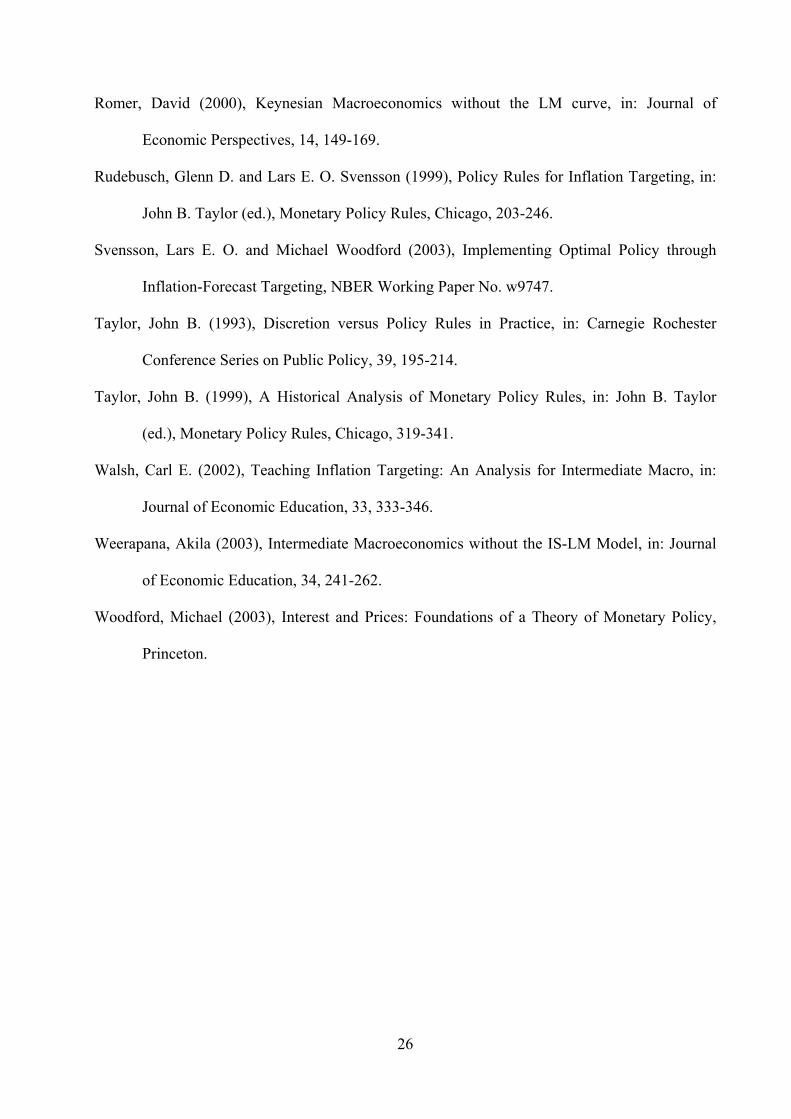
In our second scenario for flexible exchange rates we assume that the domestic inflation rate is

not affected by the exchange rate. This assumption corresponds with empirical evidence that in

the short-run the real exchange is rather unstable and mainly determined by the nominal

exchange rate (see Chart 1).

Chart 1: Nominal and real exchange rate

3.2.1 Optimal monetary policy under flexible exchange rates

As in the closed economy models it is assumed that the ultimate goal of monetary policy is to

promote welfare. In systems of flexible exchange rates this goal is usually interpreted in terms of

keeping the inflation rate close to the inflation target 0π which can be freely determined by the

central bank or the government, and stabilizing output around its potential. In the literature it is

common practice to summarize these goals by a quadratic loss function:ii

(11) ( )2 20= π − π + λL y ,

where λ denotes the central bank’s preferences. The intuition behind the quadratic loss function

is that positive and negative deviations of target values impose an identical loss on economic

agents. Large deviations from target values generate a more than proportional loss. The

popularity of the linear quadratic framework also stems from the fact that it is able to deal with

different notions of inflation targeting. If the parameter λ , which depicts the weight

policymakers attach to stabilizing the output gap compared to stabilizing the inflation rate, is

equal to zero policymakers only care about inflation. This type of inflation targeting is called

strict inflation targeting. If λ is greater than zero, the strategy is called flexible inflation

8

targeting. At the limit, if λ goes to infinity, policymakers only care about output. This

preference type is typically referred to as an output junkie.

Given the monetary policy transmission structure of the model, which runs from the real interest

rate over economic activity to the inflation rate, optimal monetary policy can be derived by

applying the following two-step procedure. First, we insert the Phillips curve (3) into the loss

function (11). Second, we minimize the modified loss function with respect to y. The solution

gives an optimal value of the output gap:

(12) ( ) 22

= − ε+ λdy

d.

Under a strategy of inflation targeting one way to conduct monetary policy is to follow an

instrument rule (Svensson and Woodford, 2003). Such a rule makes the reaction of the

instrument of monetary policy depend on all the information available at the time the instrument

is set and the structure of the economy. In our framework, the instrument rule can be derived by

inserting equation (12) into the IS equation (1) and by solving the resulting expression for r :

(13) ( )1 22

1= + ε + ε +

+ λopt a d cr q

b b bb d.

According to this reaction function the central bank responds to demand and supply shocks ( 1ε

and 2ε ), which are exogenous to the monetary policy decision, as well as to the real exchange

rate. In contrast to the domestic shocks, however, the real exchange rate is dependent on the

domestic real interest rate. This relationship is given by real UIP (equation (9)). Thus, for the

case of flexible exchange rates where UIP holds the real exchange rate in (13) has to be

substituted.

9

The major problem, however, is to approximate UIP, which prescribes a dynamic and forward-

looking law of motion of the exchange rate in a comparative-static model. In accordance with

Dornbusch (1986, Part I) we assume that the real exchange rate adjusts to its long-run level q

asymptotically, so we can write

(14) ( )1 , 0 1+ = + − < <q q g q q g ,

where 1+q is the real exchange rate in the next period and g is a key parameter determining the

average speed of adjustment.iii Combining equation (14) and the real UIP condition (9)

(augmented for risk premium shocks α ) yields an equation for the real exchange rate in terms of

the current real interest rate differential and the risk premium shock:

(15) ( )*11

= − − − α−

q q r rg

.

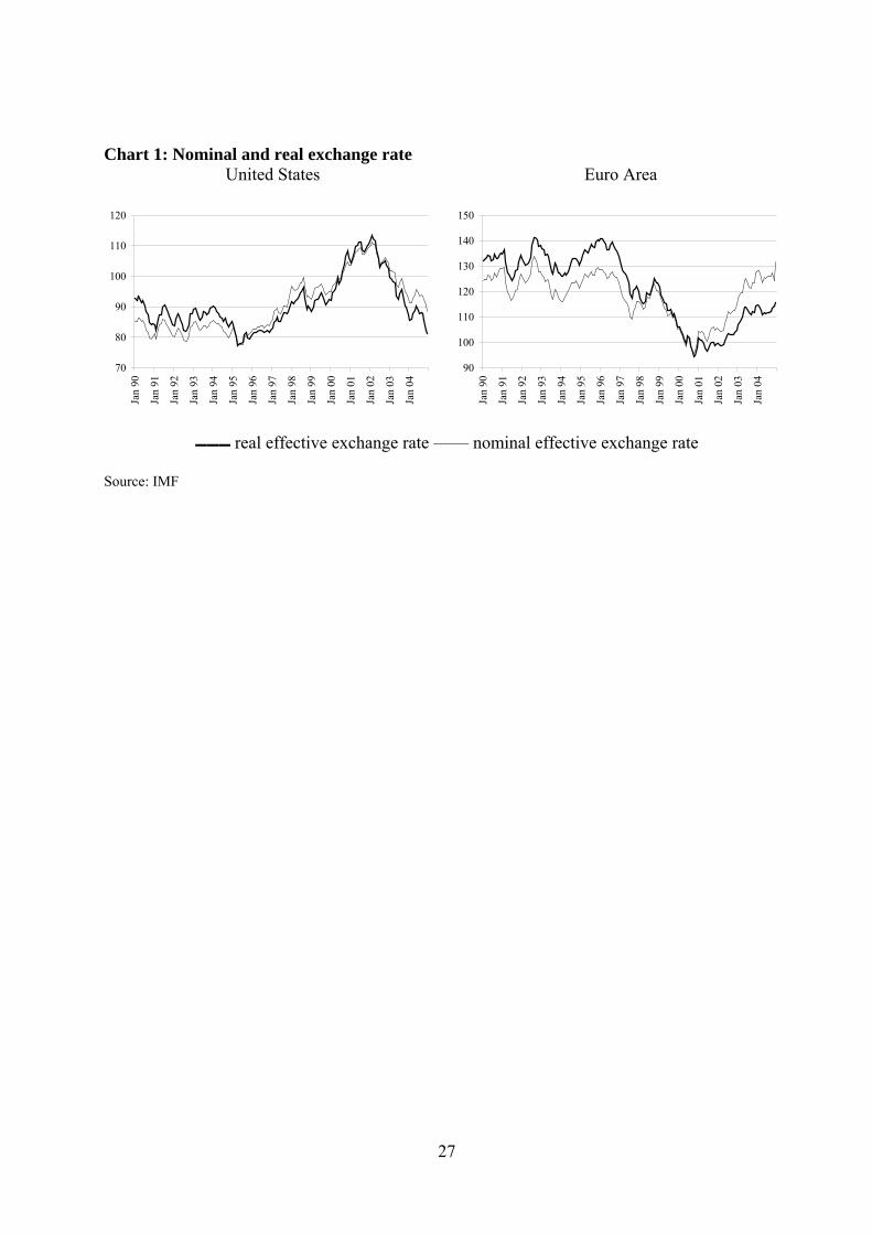
Note that we assumed that 1+∆ = −q q q . Equation (15) shows that a rise in the domestic real

interest rate will lead to an immediate real appreciation, which then is followed by a gradual

depreciation to the initial long-run equilibrium. The higher the parameter g , the lower the speed

of adjustment of the real exchange rate, and the larger the impact of real interest rate changes on

the current real exchange rate. Chart 2 shows the adjustment of the real exchange rate after an

increase of the domestic real interest rate by one percent for 0=g and 0.8g = . For simplicity

we assumed that the long-run level of the real exchange rate is equal to zero.

Chart 2: The dynamics of the real exchange rate after an increase of the domestic real interest

rate

10

For a comparative-static model, such as the one presented here, it is convenient to set 0=g .

Equation (15) then simplifies to

(16) *= − + αq r r .

Thus, the real exchange rate appreciates in a one-to-one relationship with the domestic real

interest rate.

In order to calculate the optimal interest rate rule of a central bank in a system of flexible

exchange rates where UIP holds (with the possibility of risk premium shocks) while PPP does

not hold we have to insert equation (16) into (13) and to solve the resulting equation for r (by

assuming that = optr r ):

(17) ( )( ) ( )*

1 22

1= + ε + ε + + α

+ + ++ + λopt a d cr r

b c b c b cb c d.

Equation (17) shows that real interest rate has to respond to the following types of shocks:

- domestic shocks: supply and demand shocks,

- international shocks: foreign real interest rate shocks and risk premium shocks.

The optimal interest rate response to shocks affecting the demand side ( 1ε , α , *r ) does not

depend on the central bank’s preferences λ . In the case of these shocks the central bank changes

the interest rate in a way, which guarantees that the output gap remains closed and that inflation

remains at its target level, irrespective of the preference type (see also equation (12)). Thus, as

long as shocks solely hit the demand side of the economy they do not inflict any costs on the

society. The reaction of the central bank to supply shocks 2ε depends on its preferences λ . A

central bank that only cares about inflation ( 0λ = ), requires a strong real rate response and,

accordingly, a large output gap. With an increasing λ the real interest rate response declines. In

11

equilibrium ( )*1 2 0ε = ε = α = =r the real interest rate will be given by the neutral real short-

term interest rate ( )0 /= +r a b c .

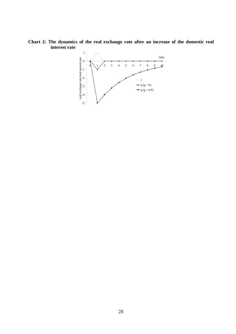
The strategy of inflation targeting under flexible exchange rates can also be presented

graphically. In the spirit of the IS-LM-AS-AD approach the graphical treatment requires two

diagrams (see Chart 3). The IS curve and the representation of monetary policy are depicted in

the y r− space. The IS curve relates the output gap to the real interest rate and the exogenous

shocks affecting the demand side of the economy. Thus, we have to replace q in equation (1) by

equation (16), which leads to a downward sloping curve in the y r− space:

(18) ( ) ( )*1= − + + + α + εy a b c r c r .

Note that the slope of the IS-curve is flatter in an open economy (1 ( )b c+ ) compared to a closed

economy (1 b ) in which 0=c . This implies that an identical increase of the real interest rate has

a weaker effect on aggregate demand in closed economy than in the open economy since in the

latter interest rate changes are accompanied by an appreciation of the real exchange rate. The

instrument rule enters as a horizontal line in the y r− space (marked by ( )r ⋅ where the dot

indicates the shift parameters of the monetary policy line 1 2, ,ε ε α and *r ). In equilibrium, at the

intersection of ( )*1 2 00r r rε = ε = α = = = and IS0, the output gap y is closed. The Phillips curve

is depicted as an upward sloping curve in the y − π space. If 0y = , inflation is at its target level.

For 1λ = the loss function of the central bank can be illustrated by circles around a bliss point in

the y − π space. The bliss point that represents the first best outcome with a loss of zero is

defined by an inflation rate π equal to the inflation target 0π and an output gap of zero. We can

derive the geometric form of the circle by transforming the loss function (11) into

12

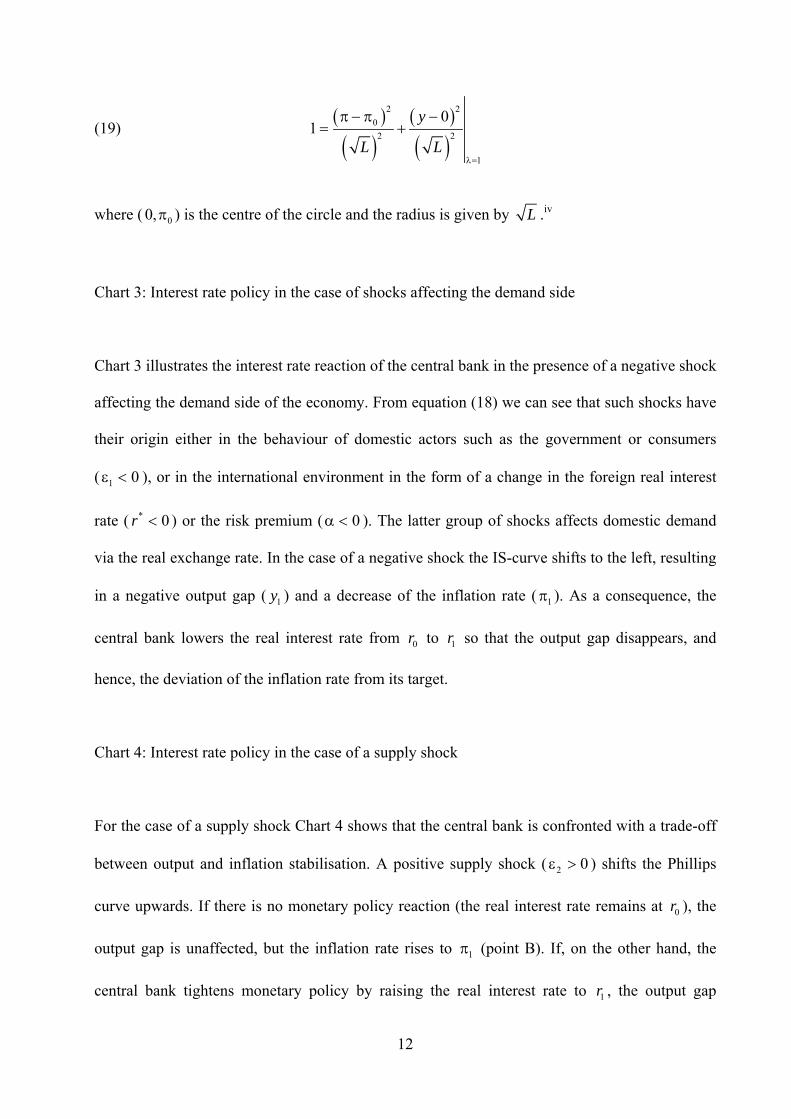
(19) ( )

( )( )

( )2 2

02 2

1

01

y

L Lλ=

π − π −= +

where ( 00,π ) is the centre of the circle and the radius is given by L .iv

Chart 3: Interest rate policy in the case of shocks affecting the demand side

Chart 3 illustrates the interest rate reaction of the central bank in the presence of a negative shock

affecting the demand side of the economy. From equation (18) we can see that such shocks have

their origin either in the behaviour of domestic actors such as the government or consumers

( 1 0ε < ), or in the international environment in the form of a change in the foreign real interest

rate ( * 0<r ) or the risk premium ( 0α < ). The latter group of shocks affects domestic demand

via the real exchange rate. In the case of a negative shock the IS-curve shifts to the left, resulting

in a negative output gap ( 1y ) and a decrease of the inflation rate ( 1π ). As a consequence, the

central bank lowers the real interest rate from 0r to 1r so that the output gap disappears, and

hence, the deviation of the inflation rate from its target.

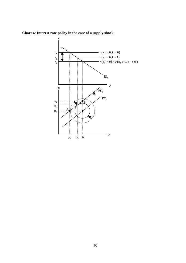
Chart 4: Interest rate policy in the case of a supply shock

For the case of a supply shock Chart 4 shows that the central bank is confronted with a trade-off

between output and inflation stabilisation. A positive supply shock ( 2 0ε > ) shifts the Phillips

curve upwards. If there is no monetary policy reaction (the real interest rate remains at 0r ), the

output gap is unaffected, but the inflation rate rises to 1π (point B). If, on the other hand, the

central bank tightens monetary policy by raising the real interest rate to 1r , the output gap

13

becomes negative, and the inflation rate falls back to its target level 0π (point A). The optimum

combination of y and π depends on the preferences λ of the central bank. If π and y are

equally weighted in the loss function, the iso-loss locus is a circle, and PC1 touches the circle at

( 2 2,π y ). In any case there is a social cost represented by the positive radius of the iso-loss circle.

3.2.2 Simple interest rate rules under flexible exchange rates

Instead of relying on all available information, a central bank can also restrict its information to a

small sub-set of directly observable variables. At the very heart of simple interest rate rules lies

the notion that they are not derived from an optimisation problem. Instead, the coefficients are

chosen ad hoc, based on the experiences and skills of the monetary policymakers.v The most

prominent version of a simple rule is the Taylor (1993) rule. According to this rule the actual real

interest rate is defined as the sum of the equilibrium real interest rate ( 0r ) and two additional

factors accounting for the actual economic situation that is assumed to be observable by

movements in the inflation rate and in the output gap:

(20) ( )0 0r r e f y= + π − π + with , 0>e f .

In our graphical analysis the Taylor rule can be represented by an upward-sloping monetary

policy (MP) line in the −y r space (see Chart 5). While variations of the output gap lead to

changes in the real interest rate, which constitute movements along the MP line, the inflation rate

represents a shift parameter.

The IS-curve is derived in the same way as in Section 3.2:

(21) ( ) ( )*1= − + + + α + εy a b c r c r .

14

In contrast to the previous section, under simple interest rate rules an explicit construction of an

aggregate demand (AD) curve in the y − π space is required, which depends on the simple

interest rate rule that is implemented by the central bank. Algebraically, the AD-curve can be

easily derived by inserting the Taylor rule (20) into the IS-curve (21), by replacing 0r with

( )+a b c , and by solving the resulting equation for π :

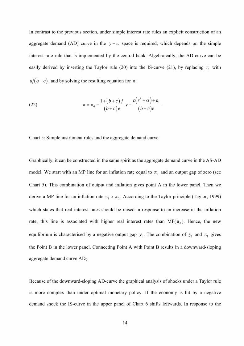
(22) ( )

( )( )

( )

*1

0

1 + α + ε+ +π = π − +

+ +

c rb c fy

b c e b c e.

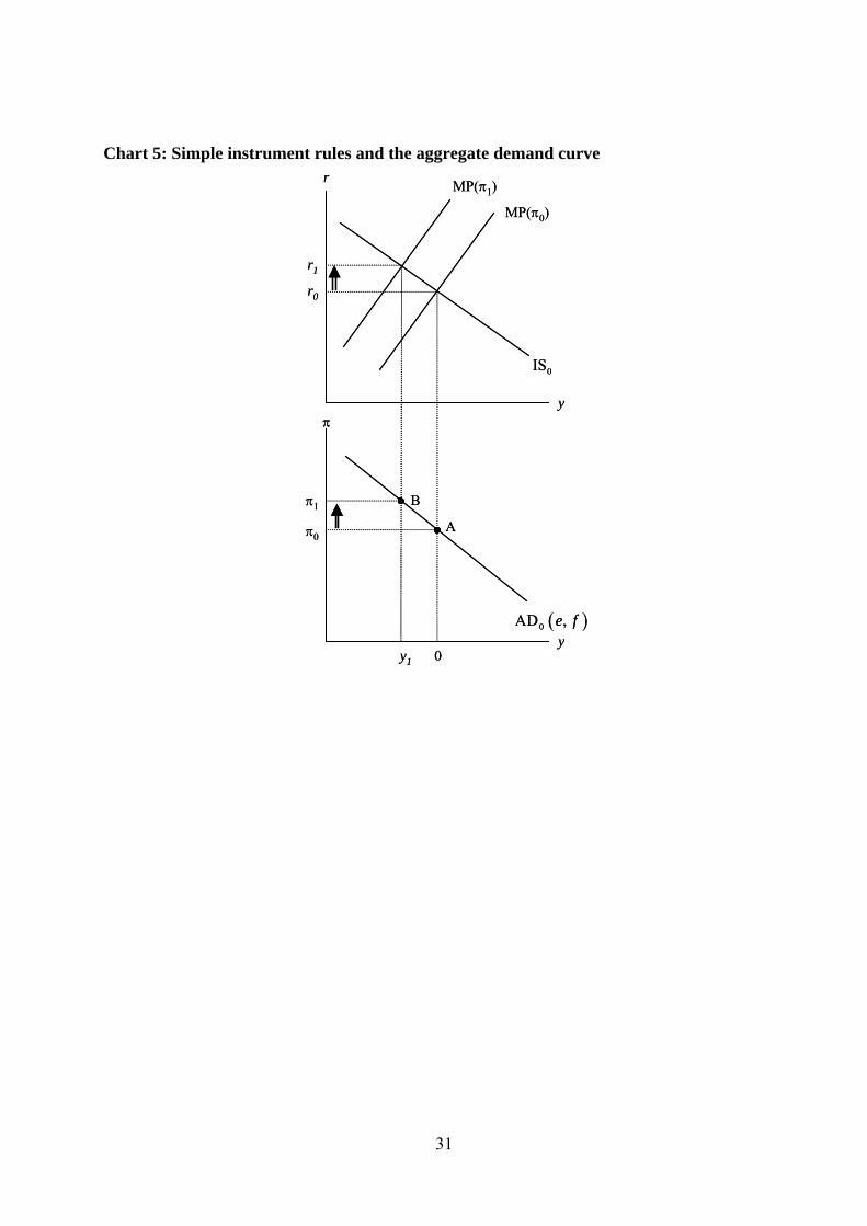
Chart 5: Simple instrument rules and the aggregate demand curve

Graphically, it can be constructed in the same spirit as the aggregate demand curve in the AS-AD

model. We start with an MP line for an inflation rate equal to 0π and an output gap of zero (see

Chart 5). This combination of output and inflation gives point A in the lower panel. Then we

derive a MP line for an inflation rate 1 0π > π . According to the Taylor principle (Taylor, 1999)

which states that real interest rates should be raised in response to an increase in the inflation

rate, this line is associated with higher real interest rates than MP( 0π ). Hence, the new

equilibrium is characterised by a negative output gap 1y . The combination of 1y and 1π gives

the Point B in the lower panel. Connecting Point A with Point B results in a downward-sloping

aggregate demand curve AD0.

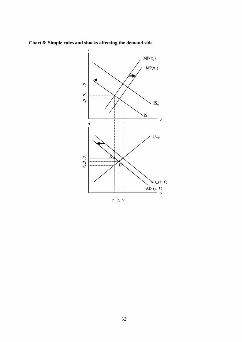
Because of the downward-sloping AD-curve the graphical analysis of shocks under a Taylor rule

is more complex than under optimal monetary policy. If the economy is hit by a negative

demand shock the IS-curve in the upper panel of Chart 6 shifts leftwards. In response to the

15

decrease of the output gap from 0 to 'y the central bank lowers real interest rates – by moving

along the MP( 0π )-line – from 0r to 'r , which leads to the output gap 'y . In the lower panel the

aggregate demand curve has to shift. Its new locus is determined by the fact that it has to go

through a point (A), which is defined by the new output gap ( 'y ) and the (so far) unchanged

inflation rate 0π . The new equilibrium is reached by the intersection of the shifted aggregate

demand curve with the unchanged Phillips-curve in point (B). It is characterized by an output

decline to 1y (which is less than 'y ) and an inflation rate 1π . The decline of the output gap from

'y to 1y and the inflation rate to 1π (instead of 'π ) is due to fact that the central bank

additionally reduces the real interest rate, because the Taylor rule requires a lower real rate as a

consequence of the decline in the inflation rate.

Chart 6: Simple rules and shocks affecting the demand side

In the upper panel this is reflected by a shift of the MP line to the right, which intersects with the

IS1 line at the same output level that results from the intersection of the AD1 line with the

Phillips curve in the lower panel. This may sound somewhat difficult but the mechanics of the

shifts are completely identical with the shifts in the IS-LM-AS-AD model in the case of the same

shock. Although in our model the decline in inflation implies an expansionary monetary impulse

because it lowers the real interest rate, in the IS-LM-AS-AD model the decrease in the price

level increases the real money stock, which also has an expansionary effect since it lowers the

nominal interest rate.

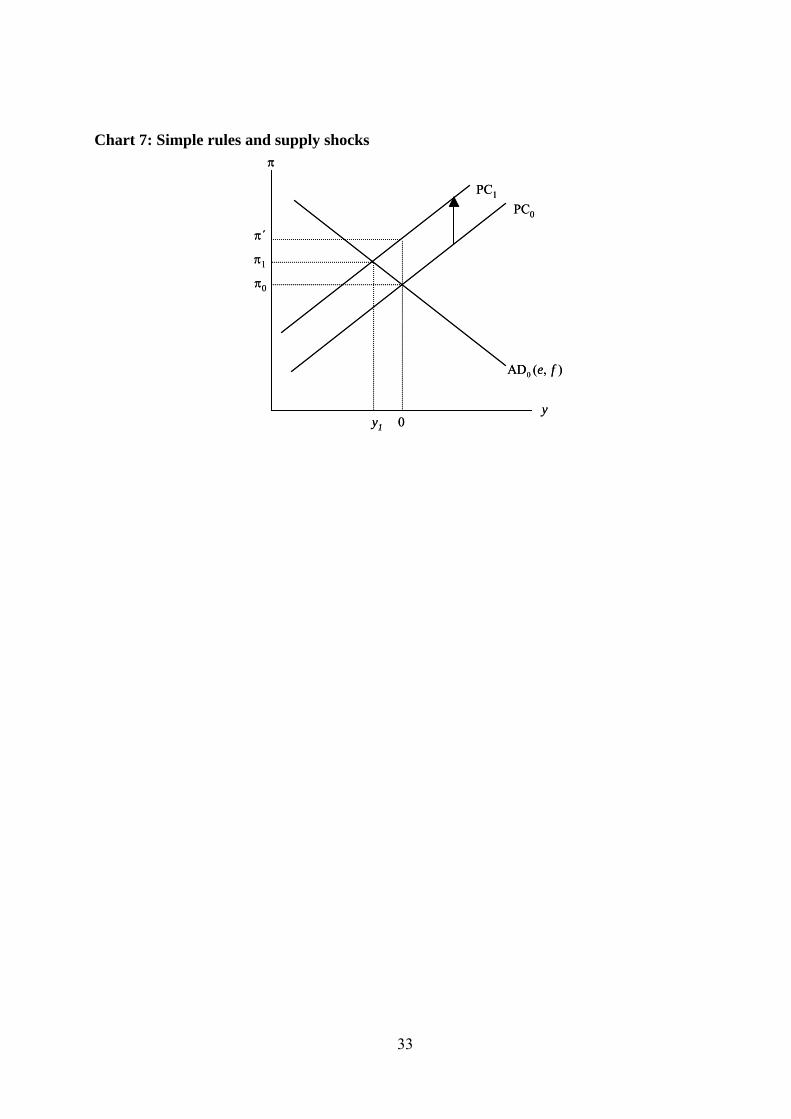
For a graphical discussion of a supply shock we only need to consider the − πy space (see Chart

7). The Phillips curve is shifted upwards which increases the inflation rate to 'π . In this case the

16

Taylor rule requires a higher real interest rate, which leads to a negative output gap 1y . The

reduced economic activity finally dampens the increase of the inflation rate to 1π .

Chart 7: Simple rules and supply shocks

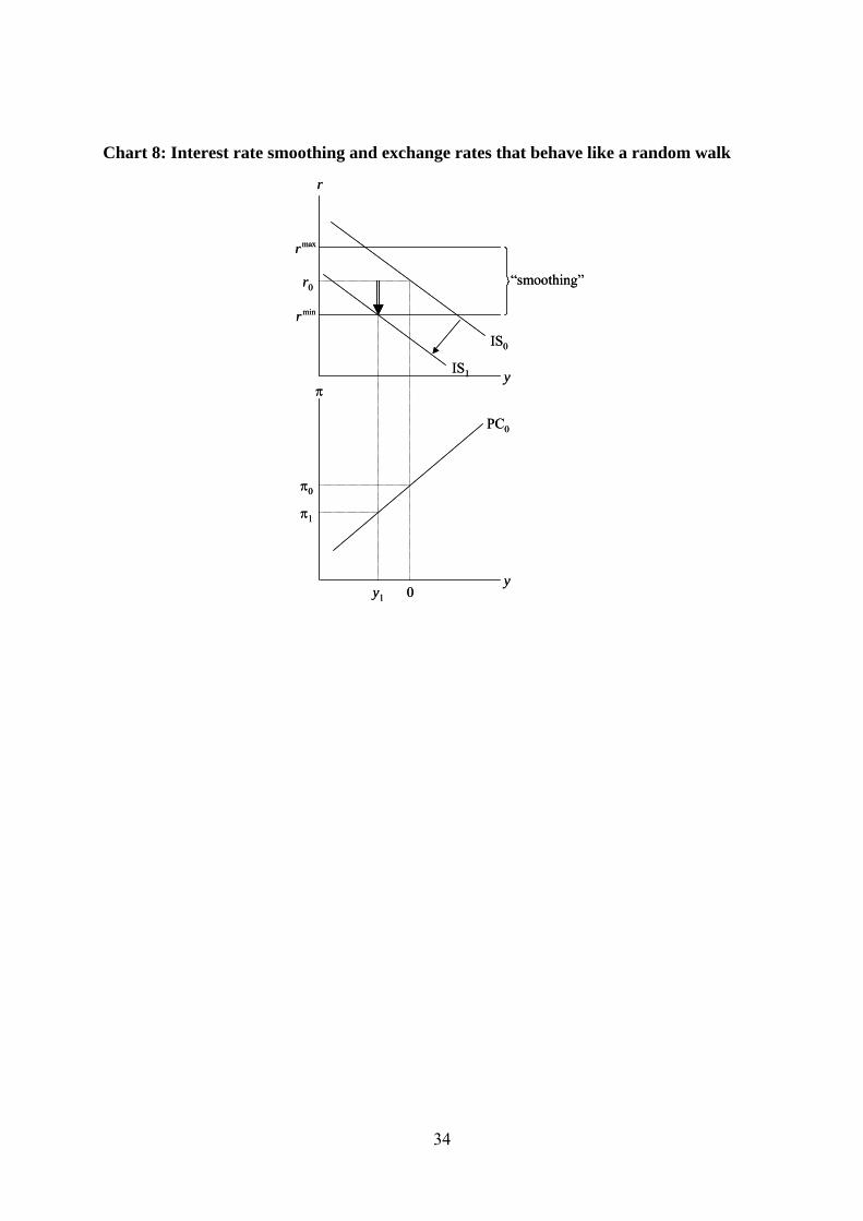
3.3 Monetary policy under flexible exchange rates that behave like a random walk

One of the main empirical findings on the determinants of exchange rates is that in a system of

flexible exchange rates no macroeconomic variable is able to explain exchange rate movements

(especially in the short and medium-run which is the only relevant time horizon for monetary

policy) and that a simple random walk out-performs the predictions of the existing models of

exchange rate determination (Meese and Rogoff, 1983). In a very simple way such random walk

behaviour can be described by

(23) = + ηq q

where η is a random white noise variable. Inserting equation (23) into (13) yields the following

optimum interest rate:

(24) ( )1 22

1= + ε + ε + η

+ λopt a d cr

b b bb d.

Random exchange rate movements constitute an additional shock to which the central bank has

to respond with its interest rate policy. At first sight, even under this scenario monetary policy

autonomy is still preserved. However, there are limitations, which depend on

- the size and the persistence of such shocks, and

- the impact of real exchange rate changes on aggregate demand, which is determined by

the coefficient c in equation (1).

17

Empirical evidence shows that the variance of real exchange rates exceeds the variance of

underlying economic variables such as money and output by far. This so-called “excess volatility

puzzle” of the exchange rate is excellently documented in the studies of Baxter and Stockman

(1989) and Flood and Rose (1995). Based on these results we assume that [ ] [ ]1η εVar Var .

Thus if a central bank would try to compensate the demand shocks created by changes in the real

exchange rate, it could generate highly unstable real interest rates. While this causes no problems

in our purely macroeconomic framework, there is no doubt that most central banks try to avoid

an excessive instability of short-term interest rates (“interest rate smoothing”) in order to

maintain sound conditions in domestic financial markets.vi If this has the consequence that the

central bank does not sufficiently react to a real exchange rate shock, the economy is confronted

with a sub-optimal outcome for the final targets y and π .

For the graphical solution the IS-curve is simply derived by inserting equation (23) into (1)

which eliminates q :

(25) 1= − + η + εy a b r c .

Exchange rate shocks η lead to a shift of the IS-curve, similar to what happens in the case of a

demand shock. In Chart 8 we introduced a smoothing band that limits the room of manoeuvre of

the central bank’s interest rate policy. In order to avoid undue fluctuations of the interest rate, the

central bank refrains from a full and optimal interest rate reaction in response to a random real

appreciation ( 0η < ) that shifts the IS-curve to the left. As a result, the shock is only partially

compensated so that the output gap and the inflation rate remain below their target levels.

Chart 8: Interest rate smoothing and exchange rates that behave like a random walk

18

4 Monetary policy under fixed exchange rates

With fixed exchange rates a central bank completely loses its leeway for a domestically oriented

interest rate policy. In order to avoid destabilising short-term capital inflows or outflows, the

central bank has to follow UIP in a very strict way. If the fixed rate system is credible, 0∆ =s

and the UIP condition simplifies to:

(26) *= + αi i .

Inserting equation (26) into (8) shows how the real interest rate is determined under fixed

exchange rates:

(27) *= + α − πr i .

4.1 Fixed exchange rates as a destabilising policy rule

As the real interest rate is only determined by foreign variables and as it depends negatively on

the domestic inflation rate, the central bank can no longer pursue an autonomous real interest

rate policy. In principle, this interest rate rule can be interpreted as a special case of a simple

interest rate rule. Equation (27) can easily be transformed into

(28) ( ) ( )( )*0 01 0= + α − π + − π − π + ⋅r i y ,

that is, a specific simple rule with 1= −e and 0=f (see equation (20) for a general definition

of simple rules). It is interesting to see that under fixed exchange rates real interest rates have to

fall when the domestic inflation rate rises. Thus, monetary policy becomes more expansive in

situations of accelerating price increases which questions the stabilizing properties of fixed

exchange rates in times of shocks.

19

This can also be shown with our graphical analysis. Since the real rate is not affected by the

domestic output gap, the monetary-policy line (MP) enters the −y r space as a horizontal line.

The IS-curve is given by:

(29) ( ) ( )*1= − + + + α + εy a b c r c r ,

which is equal to the IS curve under flexible exchange rates. The corresponding interest-rate-

rule-dependent AD-curve in the − πy space is derived in a similar way as in the case of simple

interest rate rules. By inserting the interest rate rule (27) in equation (29) we get:

(30) ( )* *1

1 ⎡ ⎤π = π + − + + α − ε⎣ ⎦+y a b r

b c.

This implies that the AD-curve has a positive slope. Compared with the negative slope of the

AD-curve under a Taylor rule (see Section 3.2.2), the positive slope reveals again the

destabilising property of the “interest rate rule” generated by fixed exchange rates. For the

graphical analysis it is important to see that

- the slopes of the IS-curve and the AD-curve have the same absolute value, but the

opposite sign;

- the slope of the AD-curve ( )1 +b c is greater than one as ( )0 1b c< + < . Thus, the AD-

curve is steeper than the Phillips curve whose slope is d and which is assumed to be

positive and smaller than one.

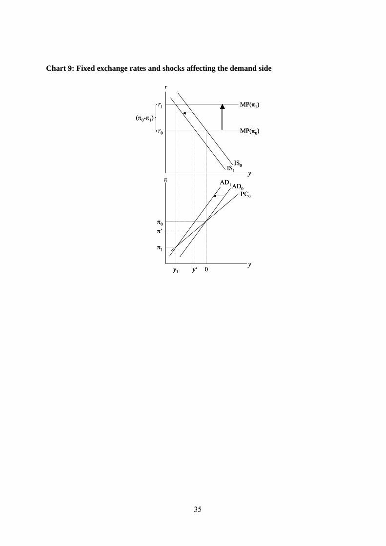
4.2 The impact of demand and supply shocks

In Chart 9 we use this framework to discuss the consequences of a negative shock that affects the

demand side of the domestic economy ( 1ε , *r , α ). The result is a shift of the IS-curve to the left.

20

Without repercussions on the real interest rate the output gap would fall to 'y and the inflation

rate to 'π . However, in a system of fixed exchange rates the initial fall in π increases the

domestic real interest rates since the nominal interest rate is kept unchanged on the level of the

foreign nominal interest rate. Thus, in a first step, we use the new output gap ( 'y ) and an

unchanged inflation rate ( 0π ) to construct the new location of the AD-curve in the − πy space.

It also shifts to the left to AD1.vii This finally leads to the new equilibrium combination ( 1 1,πy ),

which is the intersection between the Phillips curve and the new AD-curve. This equilibrium

goes along with a rise of the real interest rate from 0r to 1r , which is equal to the fall of the

inflation rate from 0π to 1π . It is obvious from Chart 9 that the monetary policy reaction in a

system of fixed exchange rates is destabilising since 1 'π < π and 1 '<y y .

Chart 9: Fixed exchange rates and shocks affecting the demand side

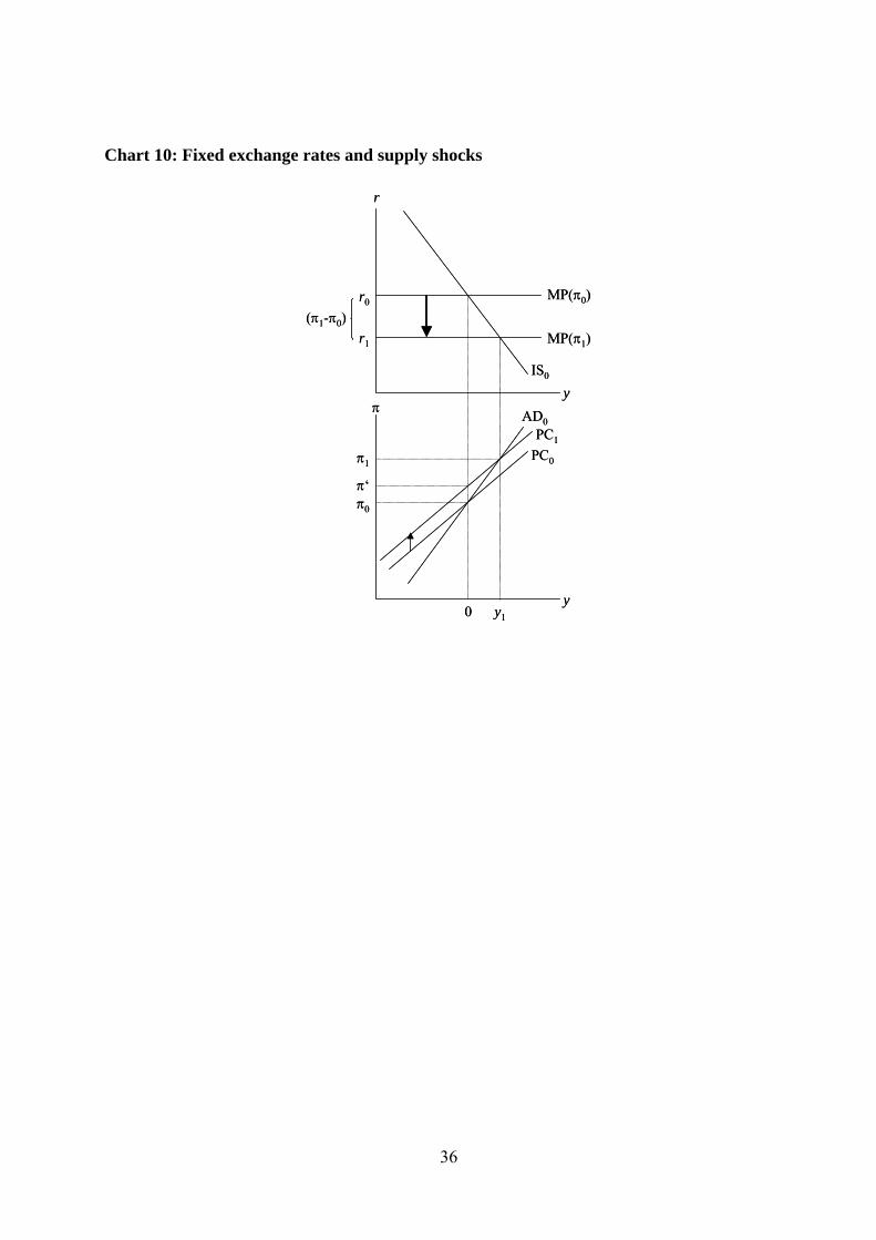
In Chart 10 we discuss the effects of a supply shock. Initially, the shock shifts the Phillips curve

upwards, which leads to a higher inflation rate ( 'π ) with an unchanged output gap. Since the rise

in inflation lowers the real interest rate, a positive output gap emerges which leads to a further

rise of π . The final equilibrium is the combination ( 1 1,πy ). Again, one can see that the “policy

rule” of fixed exchange rates has a destabilising effect as it increases the effects of the shock

compared to a situation in which there would have been no monetary policy reaction ( 0, 'π ).

Chart 10: Fixed exchange rates and supply shocks

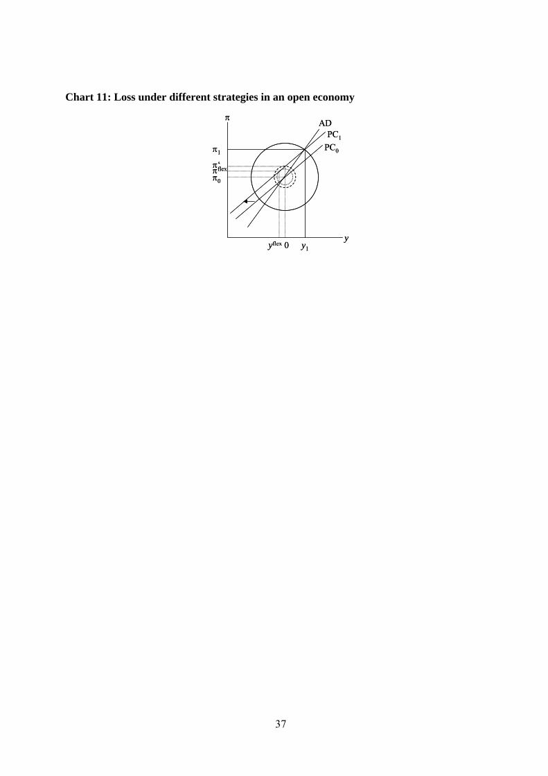
Chart 11 shows that this combination is also sub-optimal compared with the outcome a central

bank chooses under optimal policy behaviour in a system of flexible exchange rates (see Chart

21

4). Assuming again that the central bank equally weights π and y in its loss function, the dotted

circle ( flex flex,πy ) depicts the loss under flexible exchange rates. If the central bank had followed

a policy of constant real interest rates (that is absence of any policy reaction) the dashed circle

would have been realised with ( '0,π ). Under fixed exchange rates, however, the iso-loss circle

expands significantly, and the final outcome in terms of the central bank’s target variables is

( 1 1,πy ).

Chart 11: Loss under different strategies in an open economy

4.3 Fixed rates can also be stabilising

From this analysis one would be tempted to draw the conclusion that a system of fixed exchange

rates always performs poorly. However, this result is difficult to reconcile with the empirical fact

that for example countries like the Netherlands and Austria could follow a very successful

macroeconomic policy under almost absolutely fixed exchange rates in the 1980s and 1990s.

An explanation for this observation is that our analysis leaves it open how the foreign real

interest rate is determined. A stabilising movement of the domestic real interest rate can be

generated if the foreign central bank is confronted with and reacts to the same demand shocks as

the domestic economy. This was certainly the case in the Netherlands and Austria, which pegged

their currency to the D-Mark until 1998. The economies in both countries are very similar to the

German economy. Thus, in the literature on optimum currency areas the correlation of real

shocks plays a very important role (see e.g. Bayoumi and Eichengreen, 1992).

22

5 Summary and comparison with the results of the Mundell-Fleming model

For many central banks open economy considerations are of major importance for the conduct of

monetary policy. Above all the choice between absolutely fixed exchange rates (like unilateral

pegs or monetary unions) and perfectly flexible exchange rates is still a matter of debate. Today

the workhorse open economy model in intermediate textbooks is the Mundell-Fleming (MF)

model, even though our understanding of monetary policy has shifted away in recent years from

money supply rules and fixed-price models to interest rate rules and inflation targeting. This

paper presents an open economy model that ties in with the tradition of modern New Keynesian

(NK) macro models. It provides students taking an intermediate-level macroeconomics course

with a tool that allows a simple analytical and graphical analysis of monetary policy aspects

under both, fixed and flexible exchange rates.

For a summary of the open-economy version of the NK macro model it seems useful to compare

it with the main policy implications of the MF model. Under fixed exchange rates the MF model

comes to the conclusion that

- monetary policy is completely ineffective, while

- fiscal policy is more effective than in a closed-economy setting.

The NK model shows that monetary policy is not only ineffective but rather has a destabilising

effect on the domestic economy. Compared with the MF model the sources of demand shocks

can be made more explicit (above all the foreign real interest rate and the risk premium) and it is

also possible to analyse the effects of supply shocks. As far as the effects of fiscal policy are

concerned the NK model also comes to the conclusion that it is an effective policy tool, and that

it is more effective than in a closed economy. A restrictive fiscal policy has similar effects as a

23

negative demand shock so that we can use the results of Chart 9. It is obvious that the initial

effect on the output gap is magnified by the destabilising nature of the fixed exchange rate rule.

Under flexible exchange rates the MF models provides two main results:

- monetary policy is more effective than in a closed-economy setting, while

- fiscal policy becomes completely ineffective.

It is important to note that the MF model implicitly assumes that PPP is violated as it assumes

absolutely fixed prices. As far as UIP is concerned, the MF model makes the same assumption as

the baseline NK model: An increase in domestic interest rates is associated with an appreciation

of the domestic currency. For the three versions of flexible exchange rates the NK models comes

to results that are partly compatible and partly incompatible with the MF model.

For a world where PPP and UIP (long-run perspective) simultaneously hold the NK model

produces the contradictory result that there is no monetary policy autonomy with regard to the

real interest rate. Thus, the central bank is unable to cope with demand shocks. However,

because of its control over the nominal interest rate it can target the inflation rate and thus react

to supply shocks. For fiscal policy the NK model also differs from the MF model. As it assumes

an exogenously determined real interest rate, i.e. a horizontal monetary policy line, fiscal policy

has the same effects as in a closed economy. By shifting the IS-curve it can perfectly control the

output-gap and indirectly also the inflation rate.

Under a short-run perspective (UIP holds, PPP does not hold) the results of the NK model are

identical with regard to monetary policy. The central bank can control aggregate demand and the

inflation rate by the real interest rate. Fiscal policy is again effective and if one assumes that the

24

central bank does not react to actions of fiscal policy (constant real rate) it is as effective as in a

closed economy.

In the third scenario for flexible exchange rates (random walk) the results of the NK model are in

principle identical with those of the short-term perspective. However, the ability of monetary

policy to react to exchange rate shocks can be limited by the need to follow a policy of interest

rate smoothing. Thus, there can be clear limits to the promise of monetary policy autonomy

made by the MF model. Again fiscal policy remains fully effective.

In sum, the NK model shows that for flexible exchange rates a much more differentiated

approach is needed than under the MF model. Above all, the results of the MF model concerning

fiscal policy are no longer valid if monetary policy is conducted in the form of interest rate rule

instead of a monetary targeting rule on which the MF model is based. In the NK model fiscal

policy remains a powerful policy tool in all three version of flexible exchange rates, provided

that the central bank does not instantaneously off-set the fiscal impulse.

25

References

Baxter, Marianne and Alan C. Stockman (1989), Business Cycles and the Exchange-Rate

Regime: Some International Evidence, in: Journal of Monetary Economics, 23, 377-400.

Bayoumi, Tamim and Barry Eichengreen (1992), Shocking Aspects of European Monetary

Unification, CEPR Discussion Paper No. 643.

Bofinger, Peter, Eric Mayer, and Timo Wollmershauser (2005), The BMW Model: A New

Framework for Teaching Monetary Economics, in: Journal of Economic Education,

forthcoming.

Carlin, Wendy and David Soskice (2004), The 3-Equation New Keynesian Model: A Graphical

Exposition, CEPR Discussion Paper No. 4588.

Clarida, Richard, Jordi Gali, and Mark Gertler (1999), The Science of Monetary Policy: A New

Keynesian Perspective, in: Journal of Economic Literature, 37, 1661-1707.

Dornbusch, Rudi (1986), Dollars, Debts, and Deficits, Cambridge.

Flood, Robert P. and Andrew K. Rose (1995), Fixing exchange rates: A virtual quest for

fundamentals, in: Journal of Monetary Economics, 36, 3-37.

Johnson, Harry G. (1972), The Case for Flexible Exchange Rates, 1969, in: Harry G. Johnson

(ed.), Further Essays in Monetary Economics 198-222.

McCallum, Bennett T. and Edward Nelson (2000), Monetary Policy for an Open Economy: An

Alternative Framework with Optimizing Agents and Sticky Prices, in: Oxford Review of

Economic Policy, 16, 74-91.

Meese, Richard A. and Kenneth Rogoff (1983), Empirical Exchange Rate Models of the

Seventies: Do They Fit Out of Sample, in: Journal of International Economics, 14, 3-24.

26

Romer, David (2000), Keynesian Macroeconomics without the LM curve, in: Journal of

Economic Perspectives, 14, 149-169.

Rudebusch, Glenn D. and Lars E. O. Svensson (1999), Policy Rules for Inflation Targeting, in:

John B. Taylor (ed.), Monetary Policy Rules, Chicago, 203-246.

Svensson, Lars E. O. and Michael Woodford (2003), Implementing Optimal Policy through

Inflation-Forecast Targeting, NBER Working Paper No. w9747.

Taylor, John B. (1993), Discretion versus Policy Rules in Practice, in: Carnegie Rochester

Conference Series on Public Policy, 39, 195-214.

Taylor, John B. (1999), A Historical Analysis of Monetary Policy Rules, in: John B. Taylor

(ed.), Monetary Policy Rules, Chicago, 319-341.

Walsh, Carl E. (2002), Teaching Inflation Targeting: An Analysis for Intermediate Macro, in:

Journal of Economic Education, 33, 333-346.

Weerapana, Akila (2003), Intermediate Macroeconomics without the IS-LM Model, in: Journal

of Economic Education, 34, 241-262.

Woodford, Michael (2003), Interest and Prices: Foundations of a Theory of Monetary Policy,

Princeton.

27

Chart 1: Nominal and real exchange rate United States Euro Area

70

80

90

100

110

120

Jan

90

Jan

91

Jan

92

Jan

93

Jan

94

Jan

95

Jan

96

Jan

97

Jan

98

Jan

99

Jan

00

Jan

01

Jan

02

Jan

03

Jan

04

90

100

110

120

130

140

150

Jan

90

Jan

91

Jan

92

Jan

93

Jan

94

Jan

95

Jan

96

Jan

97

Jan

98

Jan

99

Jan

00

Jan

01

Jan

02

Jan

03

Jan

04

▬▬▬ real effective exchange rate —— nominal effective exchange rate

Source: IMF

28

Chart 2: The dynamics of the real exchange rate after an increase of the domestic real interest rate

-5

-4

-3

-2

-1

0

1

0 1 2 3 4 5 6 7 8 9 10

time

real

exc

hang

e ra

te/re

al in

tere

st ra

ter

q (g = 0)

q (g = 0.8)

29

Chart 3: Interest rate policy in the case of shocks affecting the demand side

π

r

y

y

π0

r0

0

PC0

y1

π1

r1

( )1 0ε =r

bliss point

( )1 0ε <r

0IS1IS

π

r

y

y

π0

r0

0

PC0

y1

π1

r1

( )1 0ε =r

bliss point

( )1 0ε <r

0IS1IS

30

Chart 4: Interest rate policy in the case of a supply shock

π

r

y

y

π0

r0

0

PC0

y2

π2

r2( ) ( )2 20 0,ε = = ε > λ → ∞r r

0IS

PC1

( )2 0, 1ε > λ =r

A

B

r1 ( )2 0, 0ε > λ =r

π1

y1

π

r

y

y

π0

r0

0

PC0

y2

π2

r2( ) ( )2 20 0,ε = = ε > λ → ∞r r

0IS

PC1

( )2 0, 1ε > λ =r

A

B

r1 ( )2 0, 0ε > λ =r

π1

y1

31

Chart 5: Simple instrument rules and the aggregate demand curve

π

r

y

y

r0

0

0IS

MP(π0)

MP(π1)

π0

π1

y1

r1

A

B

( )0AD ,e f

π

r

y

y

r0

0

0IS

MP(π0)

MP(π1)

π0

π1

y1

r1

A

B

( )0AD ,e f

32

Chart 6: Simple rules and shocks affecting the demand side

π

r

y

y

r0

0

PC0

MP(π0)

MP(π1)

π0π1

y1

r1

r´

y´

1AD ( , )e f0AD ( , )e f

0IS

1IS

π´ B

A

π

r

y

y

r0

0

PC0

MP(π0)

MP(π1)

π0π1

y1

r1

r´

y´

1AD ( , )e f0AD ( , )e f

0IS

1IS

π´ B

A

33

Chart 7: Simple rules and supply shocks π

y

π0

0

PC0

PC1

y1

π1

0AD ( , )e f

π´

π

y

π0

0

PC0

PC1

y1

π1

0AD ( , )e f

π´

34

Chart 8: Interest rate smoothing and exchange rates that behave like a random walk

π

r

y

y

π0

r0

0

PC0

maxr

minr

π1

y1

“smoothing”

IS0

IS1

π

r

y

y

π0

r0

0

PC0

maxr

minr

π1

y1

“smoothing”

IS0

IS1

35

Chart 9: Fixed exchange rates and shocks affecting the demand side

π

r

y

y

π0

r0

0

PC0

y‘

π‘

y1

π1

MP(π0)

MP(π1)r1

(π0-π1)

IS0IS1

AD0AD1

π

r

y

y

π0

r0

0

PC0

y‘

π‘

y1

π1

MP(π0)

MP(π1)r1

(π0-π1)

IS0IS1

AD0AD1

36

Chart 10: Fixed exchange rates and supply shocks

π

r

y

y

π0

r0

0

PC0

PC1

π‘

y1

π1

MP(π0)

MP(π1)r1

(π1-π0)

IS0

AD0π

r

y

y

π0

r0

0

PC0

PC1

π‘

y1

π1

MP(π0)

MP(π1)r1

(π1-π0)

IS0

AD0

37

Chart 11: Loss under different strategies in an open economy

π

y

π0

0

PC0

ADPC1

π‘

y1

π1

yflex

πflex

π

y

π0

0

PC0

ADPC1

π‘

y1

π1

yflex

πflex

38

i Following standard conventions, an increase in q is a real depreciation of the domestic currency.

ii For a microfounded derivation of the standard loss function see Woodford (2003, ch. 6).

iii The speed of adjustment can be expressed in terms of periods for a deviation of the real exchange rate from its

long-run level to decay by 50 percent: g / (1−g).

iv For λ ≠ 1, the geometric form of the loss function is an ellipse.

v Note that there is also an enormous literature on optimal simple rules that derives the coefficients of the simple rule

by minimizing the central bank’s loss function (see Rudebusch and Svensson, 1999). Although such an approach

would also be feasible within our model, we think that optimal simple rules are too complicated to be taught in

intermediate macro courses.

vi However, most models, as the one presented here, fail to integrate the variance of interest rate changes and its

consequences into a macroeconomic context.

vii In fact, the described shift of the AD-curve is only true in the case of ε1-shocks which affect the AD-curve and the

IS-curve by exactly the same extent (see equations (29) and (30)). If, however, the economy is hit by a α-shock or a

r*-shock, the AD-curve shifts by a larger amount than the IS-curve as b is typically greater than c.