Teaching Multivariate Analysis to Business-Major Students

Wing-Keung Wong and Teck-Wong Soon - Kent Ridge, Singapore

1. Introduction

During the last two or three decades, multivariate statistical analysis has become increasingly popular. The theory has made great progress, and with the rapid advances in computer technology, routine applications of multivariate statistical methods are imple- mented in several statistical software packages, making it simple even for the novice to undertake fairly sophisticated multivariate statistical analysis of data at their disposal.

While this is certainly a welcome development, we find, on the other hand, that many users of statistical packages are unable to appreciate, what they are doing, and this is particularly true for multivariate statistical methods. With the increasing use of multivariate statistical methods by business analysts, it is important for business-major students to develop an understanding of multivariate statistical methods: Even though business executives are not generally required to undertake sophisticated statistical analysis themselves, they are often presented with reports and articles based on such analysis. Furthermore, many executives have heard about these techniques and would like to use them as analytic and decision support tools.

The traditional approach to the teaching of multivariate statistical analysis, as exemplified by Anderson (1958), relies heavily on advanced matrix mathematics. On the other hand, Hury and Riedwyl(1988) suggest that it is possible to understand most of the basic ideas underlying multivariate statistical analysis without a mastery of such mathematics, provided that these are conveyed with the help of real data sets. Since most business data do not follow the usual normality assumption, there are often (possibly severe) limitations in the use of some of the standard multivariate statistical techniques. Real data sets are therefore required not only to illustrate the statistical techniques concerned, but also to clarify the assumptions needed for these techniques to be valid.

In this paper, we propose a non-mathematical data-driven approach for teaching multivariate statistical methods to business-major students. Despite this, we are mindful of the need for students to know some basic linear algebra and univariate statistical concepts. Such basic knowledge provides students with the foundation necessary for the application of the appropriate multivariate statistical procedures and for the interpretation of results.

Session B5 343

ICOTS 3, 1990: Wing-Keung Wong and Teck-Wong Soon

2. Business data and the approach to analyse them

Business data sets are usually large and undifferentiated. They are therefore generally closer to data encountered in the social sciences and differ somewhat from the more precise data encountered in the physical and natural sciences. Large and undifferentiated data sets contain so many inter-relationships that it is virtually impossible to make sense of them without fust arriving at a summary description. Multivariate statistical analysis, when applied to such data sets, should allow us to "explore" the data sets with a view to discovering, describing and understanding the major inter-relationships. While multivariate statistical techniques allow us to analyse, verify, test, and prove various hypotheses, it should be emphasised that with a large undifferentiated data set, we should, at least in the initial stages, be less involved with building a specific statistical model, or with the formal procedures of statistical inference. Thus, when teaching multivariate statistical analysis to business-major students, we should concentrate on the descriptive techniques rather than on the theory of the multivariate normal distribution, beginning with simple univariate statistical analysis leading to standard multivariate techniques such as principal component analysis, factor analysis, and cluster analysis which are applicable when the data is measured on a continuous or interval scale. Once the basic ideas have been conveyed, it would be a simple matter to introduce students to other related techniques, such as correspondence analysis and multi-dimensional scaling.

3. Illustrative example

To illustrate the approach outlined above, we consider the sample data set 'CARDATA' provided with the computer package STATGWHICS. The data set comprises 155 observations with 11 variables as follows: mpg, cylinders, displace, horsepower, accel, year, weight, origin, make, model and price. This data set is small enough for most computer packages to handle and large enough to approximate the type of data encountered in practice. Faced with such a data set, students are generally at a loss to know how to begin to analyse it, particularly when the objectives of the analysis have not been specified.

An obvious approach would be to begin by examining each of the variables in turn. Such an initial examination of the data has the merit of enabling students to obtain a better feel for the data. For example, on examining the variable mpg, we might consider the summary statistics tabulated in Table 1.

TABLE 1 Summary statistics for mpg

Number of Observations 154 Mean 28.79 Standard Deviation 7.37 Coefficient of Variation 25.62

Session B5

ICOTS 3, 1990: Wing-Keung Wong and Teck-Wong Soon

To enable students to familiarise themselves with the data, more elaborate univariate analysis can be undertaken. For example, students may construct histograms, plot stem-and-leaf diagrams, etc. Note also that because some variables may have missing values, the total number of observations reported may be less than 155.

Once the initial examination of data has begun, students might be led to raise further questions. For example, how does rnpg vary with other variables? If the other variable in question is a classifying (i.e. nominal-scaled) variable, the observations can be grouped before analysis. As an illustration, consider the case when the other variable is origin. Table 2 presents the summary statistics.

TABLE 2 Summary statistics for mpg by origin

United States Europe Japan

Number of Observations 85 2 5 44 Mean 25.26 32.55 33.48 Standard Deviation 6.12 8.18 5.27 Coefficient of Variation 24.22 25.13 15.75

These summary statistics suggest that Japanese cars with the highest rnpg are more economical than American or European cars. Students will then be led naturally to consider the possible reasons for this. Is it the case that Japanese cars are smaller or less powerful? Consideration of such questions will lead them to examine the variables weight and horsepower. Summary statistics presented in tables similar to Table 2 suggest that it is indeed the case that Japanese cars are lighter (i.e. smaller) and less powerful.

3.1 Regression and correlation analysis

The simple initial examination of data described above will prompt students to consider the relationship between two or more variables. They now know that Japanese cars are more fuel-economical because they are lighter and less powerful. Students will then be led to consider the relationship between fuel consumption, rnpg and weight or horsepower. The suggestion of plotting a scatterplot of rnpg against weight or horse- power can then be given. Students may then attempt to draw a "line of best fit" through the scatterplot. Figure 1, which shows the result of this exercise, indicates that rnpg decreases as weight increases. Students could then be asked to consider how best to fit the line and thus led to "least squares estimation", obtaining the line of best fit to be:

mpg = 55.89 - 0.0101 x weight

suggesting that for every lb increase in weight, the fuel consumption decreases by 0.01 mpg. Furthermore, students can be led to ask how much of the variation of rnpg can be explained by the variable weight. This leads naturally to R~ which is the proportion of the variation of the variable rnpg that is "explained" by weigh!. In this case,

Session B5

ICOTS 3, 1990: Wing-Keung Wong and Teck-Wong Soon

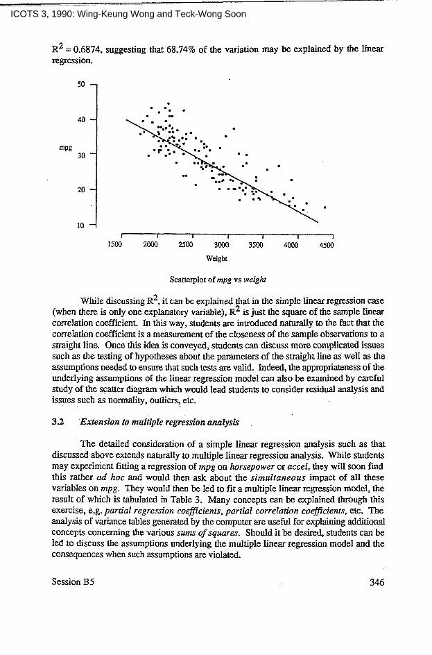
R2 = 0.6874, suggesting that 68.74% of the variation may be explained by. the linear regression.

I I I 1 1 I 1 1500 2000 2500 3000 3500 4000 4500

Weight

Scatterplot of mpg vs weight

While discussing R2, it can be explained that in the simple linear regression case (when there is only one explanatory variable), R2 is just the square of the sample linear correlation coefficient. In this way, students are introduced naturally to the fact that the correlation coefficient is a measurement of the closeness of the sample observations to a straight line. Once this idea is conveyed, students can discuss more complicated issues such as the testing of hypotheses about the parameters of the straight line as well as the assumptions needed to ensure that such tests are valid. Indeed, the appropriateness of the underlying assumptions of the linear regression model can also be examined by careful study of the scatter diagram which would lead students to consider residual analysis and issues such as normality, outliers, etc.

3 3 Extension to multiple regression analysis

The detailed consideration of a simple linear regression analysis such as that discussed above extends naturally to multiple linear regression analysis. While students may experiment fitting a regression of mpg on horsepower or accel, they will soon find this rather ad hoc and would then ask about the simultaneous impact of all these variables on mpg. They would then be led to fit a multiple linear regression model, the result of which is tabulated in Table 3. Many concepts can be explained through this exercise, e.g. partial regression coeficients, partial correlation coefficients, etc. The analysis of variance tables generated by the computer are useful for explaining additional concepts concerning the various s u m ofsquares. Should it be desired, students can be led to discuss the assumptions underlying the multiple linear regression model and the consequences when such assumptions are violated.

Session B5 346

ICOTS 3, 1990: Wing-Keung Wong and Teck-Wong Soon

While it may be argued that multiple regression analysis is not really multi- variate analysis, we are of the view that many useful concepts can be introduced in the manner we discuss. Sound understanding of such concepts is necessary as a prelude to the understanding of more complicated multivariate analytic techniques. Consideration of multiple regression analysis allows a natural introduction to the idea of the covariance or correlation matrix which is the basis of the standard multivariate analytic techniques such as principal components analysis and factor analysis. Likewise, linear discriminant analysis can be naturally related to multiple regression analysis.

TABLE 3 Regression of mpg on weight, displace, horsepower and accel

Variable Estimated Coefficient Standard Error It-value1

Intercept 52.8868 weight -0.0103 0.0017 6.06 displace 0.0239 0.01 17 2.04 horsepower -0.0709 0.0350 2.03 accel 0.3711 0.2036 1.82

R~ = 0.7346 Note: Because of missing observations, this regression is based on 150 observations.

3 3 Discriminant analysis

Multiple regression analysis presupposes that we are interested in a single response variable which is dependent on a number of independent or explanatory variables (regressors). Under multiple regression, the regressors are assumed fmed, or, if not fixed, inferences are conditioned on the values of the regressors. However, there are many multivariate problems in which all (or almost all) the variables are random variables, i.e. they are allowed to vary. Suppose, for example, we wish to discriminate between American and Japanese cars on the basis of observed values of the various variables. An obvious approach is to use multiple regression analysis with the origin as the dependent variable. Such an approach was developed by Fisher (1936). Since origin is a classification variable, we can in fact run the regression directly. However, despite the apparent similarity between multiple regression analysis and discriminant analysis, they are, in fact, conceptually different. In discriminant analysis, the "dependent" var- iable origin is fixed while the "independent" variables are random, i.e. they are allowed to vary. The result obtained with a stepwise regression of origin on mpg, weight. horsepower, accel, displace and price is, after eliminating insignificant coefficients:

origin = 3.65287 - 0.0092 x weight + 0.00012 xprice

with R~ = 0.3542, suggesting that a linear combination of weight and price will discriminate between American and Japanese cars. What should this linear combin- ation be? Obviously, the coefficients of the linear combination should be related to the

Session B5 347

ICOTS 3, 1990: Wing-Keung Wong and Teck-Wong Soon

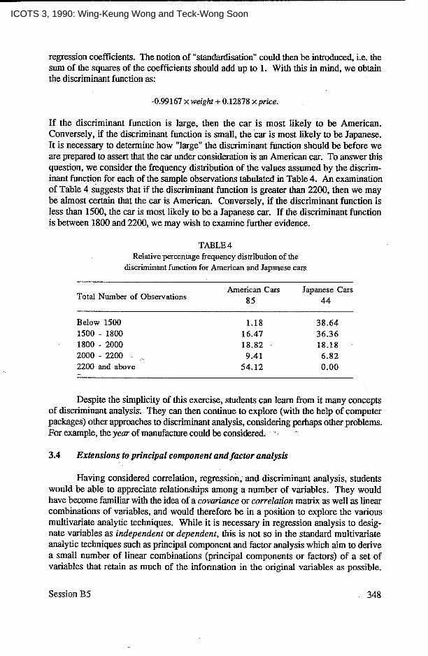
regression coefficients. The notion of "standardisation" could then be introduced, i.e. the sum of the squares of the coefficients should add up to 1. With this in mind, we obtain the discriminant function as:

-0.99167 x weight + 0.12878 xprice.

If the discriminant function is large, then the car is most likely to be American. Conversely, if the discriminant function is small, the car is most likely to be Japanese. It is necessary to determine how "large" the discriminant function should be before we are prepared to assert that the car under consideration is an American car. To answer this question, we consider the frequency distribution of the values assumed by the discrim- inant function for each of the sample observations tabulated in Table 4. An examination of Table 4 suggests that if the discriminant function is greater than 2200, then we may be almost certain that the car is American. Conversely, if the discriminant function is less than 1500, the car is most likely to be a Japanese car. If the discriminant function is between 1800 and 2200, we may wish to examine further evidence.

TMLE 4 Relative percentage frequency distribution of the

discriminant function for American and Japanese cars

American Cars Japanese Cars Total Number of Observations 85 44

Below 1500 1.18 38.64 1500 - 1800 16.47 36.36 1800 - 2000 18.82 18.18 2000 - 2200 - 9.41 6.82 2200 and above - 54.12 0.00

Despite the simplicity of this exercise, students can learn from it many concepts of discriminant analysis. They can then continue to explore (with the help of computer packages) other approaches to discriminant analysis, considering perhaps other problems. For example, the year of manufacture could be considered. .

3.4 Extensions to principal component and factor analysis

Having considered correlation, regression; and discriminant analysis, students would be able to appreciate relationships among a number of variables. They would have become familiar with the idea of a covariance or correlation matrix as well as linear combinations of variables, and would therefore be in a position to explore the various multivariate analytic techniques. While it is necessary in regression analysis to desig- nate variables as independent or dependent, this is not so in the standard multivariate analytic techniques such as principal component and factor analysis which aim to derive a small number of linear combinations (principal components or factors) of a set of variables that retain as much of the information in the original variables as possible.

Session B5 348

ICOTS 3, 1990: Wing-Keung Wong and Teck-Wong Soon

Such techniques are especially useful for summarising data and detecting linear relation- ship, and in exploratory data analysis. While principal component and factor analysis can be explained much more concisely and precisely in the language of matrix algebra (i.e. in terms of eigenvalues and eigenvectors), the basic concepts can be illustrated fairly easily to the non-mathematically inclined business-major students through an example.

For this purpose the same example can be used, building on students' familiarity with the example and their understanding and interpretation of results. For example, the first factor in a factor analysis of the above data exhibits a heavy loading in weight, horsepower, displace and mpg. These variables are related to the bulk of the car. The second factor exhibits a heavy loading in accel, a measure of speed, and the third in price. Although such interpretations appear natural and intuitive, they have nevertheless attracted considerable confusion and criticism. Students interested in such matters can be referred to books such as Gould (1981).

4. Conclusion

Statistical concepts are generally abstract and difficult for students, particularly business-major students who are not so mathematically inclined. Multivariate statistical analyses involving several variables are no less abstract, and are often expressed in terms of advanced matrix mathematics. We have therefore proposed and demonstrated a non- mathematical, data-driven approach for the teaching of such students. The irnplement- ation of this approach presupposes the availability of appropriate statistical packages and adequate computing facilities. The teacher can present a separate analysis at each lecture and discuss the results with the students who can be requested to undertake similar analyses on their own. Students learning multivariate statistical analysis through such an approach will not only be able to appreciate the basic concepts underlying multi- variate statistical analysis, but will also be able to confidently interpret the results of these analyses. Moreover, they will have the opportunity to manage a fairly large data set such as those most likely to be encountered in practice.

References

Anderson. T W (1958) An Introduction to Multivariate Statistical Analysis. John Wiley & Sons, London.

Fisher. R A (1936) The use of multiple measurements in taxonomic problems. Annals of Eugenics 7. 179-188.

Flury, Bernhard and Riedwyl, Hans (1988) Multivariate Statistics : A Practical Approach. Chapman and Hall, London.

Gnanadesikan, R (1977), Methods for Statistical Data Analysis of Multivariate Obser- vations. John Wiley & Sons. New York.

Gould, S J (1981) The Misrneasure of Man. W W Norton & Co, New York. Kaciak, Eugene and Koczkodaj, Waldemar W (1989) A spreadsheet approach to principal

components analysis. Journal of Microcomputer Applications 12, 281-291. Rao, C R (1964) The use and interpretation of principal component analysis in applied

research. Sankya A 26, 329-358.

Session B5 349

ICOTS 3, 1990: Wing-Keung Wong and Teck-Wong Soon