UNIT-I

Introduction

1.1 Introduction

The TCP/IP protocol suite allows computers of all sizes, from many different computer vendors, running totally different operating systems, to communicate with each other. It is quite amazing because its use has far exceeded its original estimates. What started in the late 1960s as a government-financed research project into packet switching networks has, in the 1990s, turned into the most widely used form of networking between computerrs. It is truly an open system in that the definition of the protocol suite and many of its implementations are publicly available at little or no charge. It forms the basis for what is called the worldwide Internet, or the Internet, a wide area network (WAN) of more than one million computers that literally spans the globe.

This chapter provides an overview of the TCP/IP protocol suite, to establish an adequate background for the remaining chapters. For a historical perspective on the early development of TCP/IP see [Lynch 1993].

1.2 Layering

Networking protocols are normally developed in layers, with each layer responsible for a different facet of the communications. A protocol suite, such as TCP/IP, is the combination of different protocols at various layers. TCP/IP is normally considered to be a 4-layer system, as shown in Figure 1.1.

Application Telnet, FTP, e-mail, etc.

Transport TCP, UDP

Network IP, ICMP, IGMP

Link device driver and interface card

Figure 1.1 The four layers of the TCP/IP protocol suite.

Each layer has a different responsibility.

1. The link layer, sometimes called the data-link layer or network interface layer, normally includes the device driver in the operating system and the corresponding network interface card in the computer. Together they handle all the hardware details of physically interfacing with the cable (or whatever type of media is being used).

2. The network layer (sometimes called the internet layer) handles the movement of packets around the network. Routing of packets, for example, takes place here. IP (Internet Protocol), ICMP (Internet Control Message Protocol), and IGMP (Internet Group Management Protocol) provide the network layer in the TCP/IP protocol suite.

3. The transport layer provides a flow of data between two hosts, for the application layer above. In the TCP/IP protocol suite there are two vastly different transport protocols: TCP (Transmission Control Protocol) and UDP (User Datagram Protocol).

TCP provides a reliable flow of data between two hosts. It is concerned with things such as dividing the data passed to it from the application into appropriately sized chunks for the network layer below, acknowledging received packets, setting timeouts to make certain the other end acknowledges packets that are sent, and so on. Because this reliable flow of data is provided by the transport layer, the application layer can ignore all these details.

UDP, on the other hand, provides a much simpler service to the application layer. It just sends packets of data called datagrams from one host to the other, but there is no guarantee that the datagrams reach the other end. Any desired reliability must be added by the application layer.

There is a use for each type of transport protocol, which we'll see when we look at the different applications that use TCP and UDP.

4. The application layer handles the details of the particular application. There are many common TCP/IP applications that almost every implementation provides:

o Telnet for remote login,

o FTP, the File Transfer Protocol,

o SMTP, the Simple Mail Transfer protocol, for electronic mail,

o SNMP, the Simple Network Management Protocol,

and many more, some of which we cover in later chapters.

If we have two hosts on a local area network (LAN) such as an Ethernet, both running FTP, Figure 1.2 shows the protocols involved.

Figure 1.2 Two hosts on a LAN running FTP.

We have labeled one application box the FTP client and the other the FTP server. Most network applications are designed so that one end is the client and the other side the server. The server provides some type of service to clients, in this case access to files on the server host. In the remote login application, Telnet, the service provided to the client is the ability to login to the server's host.

Each layer has one or more protocols for communicating with its peer at the same layer. One protocol, for example, allows the two TCP layers to communicate, and another protocol lets the two IP layers communicate.

On the right side of Figure 1.2 we have noted that normally the application layer is a user process while the lower three layers are usually implemented in the kernel (the operating system). Although this isn't a requirement, it's typical and this is the way it's done under Unix.

There is another critical difference between the top layer in Figure 1.2 and the lower three layers. The application layer is concerned with the details of the application and not with the movement of data across the network. The lower three layers know nothing about the application but handle all the communication details.

We show four protocols in Figure 1.2, each at a different layer. FTP is an application layer protocol, TCP is a transport layer protocol, IP is a network layer protocol, and the Ethernet protocols operate at the link layer. The TCP/IP protocol suite is a combination of many protocols. Although the commonly used name for the entire protocol suite is TCP/IP, TCP and IP are only two of the protocols. (An alternative name is the Internet Protocol Suite.)

The purpose of the network interface layer and the application layer are obvious-the former handles the details of the communication media (Ethernet, token ring, etc.) while

the latter handles one specific user application (FTP, Telnet, etc.). But on first glance the difference between the network layer and the transport layer is somewhat hazy. Why is there a distinction between the two? To understand the reason, we have to expand our perspective from a single network to a collection of networks.

One of the reasons for the phenomenal growth in networking during the 1980s was the realization that an island consisting of a stand-alone computer made little sense. A few stand-alone systems were collected together into a network. While this was progress, during the 1990s we have come to realize that this new, bigger island consisting of a single network doesn't make sense either. People are combining multiple networks together into an internetwork, or an internet. An internet is a collection of networks that all use the same protocol suite.

The easiest way to build an internet is to connect two or more networks with a router. This is often a special-purpose hardware box for connecting networks. The nice thing about routers is that they provide connections to many different types of physical networks: Ethernet, token ring, point-to-point links, FDDI (Fiber Distributed Data Interface), and so on.

TCP/IP Layering

There are more protocols in the TCP/IP protocol suite. Figure shows some of the additional protocols that we talk about in this text.

Figure 1.4 Various protocols at the different layers in the TCP/IP protocol suite.

TCP and UDP are the two predominant transport layer protocols. Both use IP as the network layer.

TCP provides a reliable transport layer, even though the service it uses (IP) is unreliable. UDP sends and receives datagrams for applications. A datagram is a unit of information (i.e., a certain number of bytes of information that is specified by the sender) that travels from the sender to the receiver. Unlike TCP, however, UDP is unreliable. There is no guarantee that the datagram ever gets to its final destination.

IP is the main protocol at the network layer. It is used by both TCP and UDP. Every piece of TCP and UDP data that gets transferred around an internet goes through the IP layer at both end systems and at every intermediate router. In Figure we also show an application accessing IP directly. This is rare, but possible.

ICMP is an adjunct to IP. It is used by the IP layer to exchange error messages and other vital information with the IP layer in another host or router. Although ICMP is used primarily by IP, it is possible for an application to also access it.

IGMP is the Internet Group Management Protocol. It is used with multicasting: sending a UDP datagram to multiple hosts. We describe the general properties of broadcasting (sending a UDP datagram to every host on a specified network) and multicasting

ARP (Address Resolution Protocol) and RARP (Reverse Address Resolution Protocol) are specialized protocols used only with certain types of network interfaces (such as Ethernet and token ring) to convert between the addresses used by the IP layer and the addresses used by the network interface.

1.4 Internet Addresses

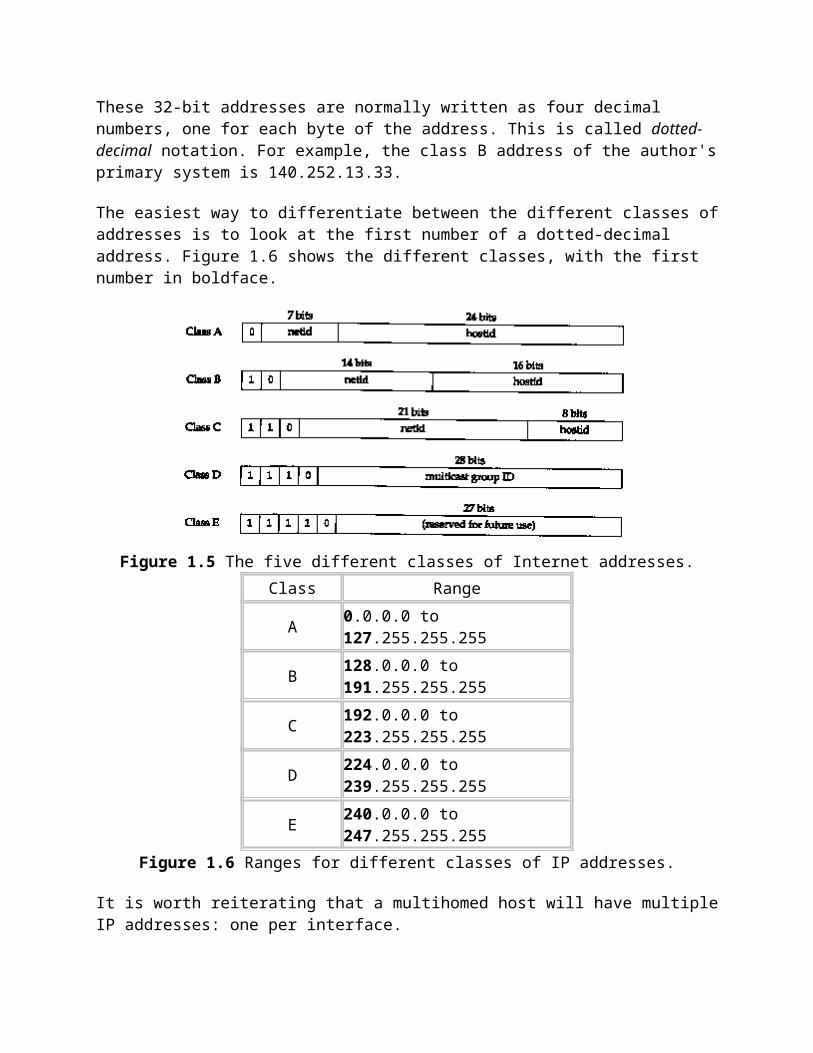
Every interface on an internet must have a unique Internet address (also called an IP address). These addresses are 32-bit numbers. Instead of using a flat address space such as 1, 2, 3, and so on, there is a structure to Internet addresses. Figure 1.5 shows the five different classes of Internet addresses.

These 32-bit addresses are normally written as four decimal numbers, one for each byte of the address. This is called dotted-decimal notation. For example, the class B address of the author's primary system is 140.252.13.33.

The easiest way to differentiate between the different classes of addresses is to look at the first number of a dotted-decimal address. Figure 1.6 shows the different classes, with the first number in boldface.

Figure 1.5 The five different classes of Internet addresses.

Class Range

A 0.0.0.0 to 127.255.255.255

B 128.0.0.0 to 191.255.255.255

C 192.0.0.0 to 223.255.255.255

D 224.0.0.0 to 239.255.255.255

E 240.0.0.0 to 247.255.255.255

Figure 1.6 Ranges for different classes of IP addresses.

It is worth reiterating that a multihomed host will have multiple IP addresses: one per interface.

Since every interface on an internet must have a unique IP address, there must be one central authority for allocating these addresses for networks connected to the worldwide Internet. That authority is the Internet Network Information Center, called the InterNIC. The InterNIC assigns only network IDs. The assignment of host IDs is up to the system administrator.

Registration services for the Internet (IP addresses and DNS domain names) used to be handled by the NIC, at nic.ddn.mil. On April 1, 1993, the InterNIC was created. Now the NIC handles these requests only for the Defense Data Network (DDN). All other Internet users now use the InterNIC registration services, at rs.internic.net.

There are actually three parts to the InterNIC: registration services (rs.internic.net), directory and database services (ds.internic.net), and information services (is.internic.net). See Exercise 1.8 for additional information on the InterNIC.

There are three types of IP addresses: unicast (destined for a single host), broadcast (destined for all hosts on a given network), and multicast (destined for a set of hosts that belong to a multicast group).

The Domain Name System

Although the network interfaces on a host, and therefore the host itself, are known by IP addresses, humans work best using the name of a host. In the TCP/IP world the Domain Name System (DNS) is a distributed database that provides the mapping between IP addresses and hostnames.

For now we must be aware that any application can call a standard library function to look up the IP address (or addresses) corresponding to a given hostname. Similarly a function is provided to do the reverse lookup-given an IP address, look up the corresponding hostname.

Most applications that take a hostname as an argument also take an IP address. When we use the Telnet client example, one time we specify a host-name and another time we specify an IP address.

1.6 Encapsulation

When an application sends data using TCP, the data is sent down the protocol stack, through each layer, until it is sent as a stream of bits across the network. Each layer adds information to the data by prepending headers (and sometimes adding trailer information) to the data that it receives. Figure 1.7 shows this process. The unit of data that TCP sends to IP is called a TCP segment. The unit of data that IP sends to the network interface is called an IP datagram. The stream of bits that flows across the Ethernet is called a frame.

The numbers at the bottom of the headers and trailer of the Ethernet frame in Figure 1.7 are the typical sizes of the headers in bytes. We'll have more to say about each of these headers in later sections.

A physical property of an Ethernet frame is that the size of its data must be between 46 and 1500 bytes. We'll encounter this minimum in Section 4.5 and we cover the maximum in Section 2.8.

All the Internet standards and most books on TCP/IP use the term octet instead of byte. The use of this cute, but baroque term is historical, since much of the early work on TCP/IP was done on systems such as the DEC-10, which did not use 8-bit bytes. Since almost every current computer system uses 8-bit bytes, we'll use the term byte in this text.

To be completely accurate in Figure 1.7 we should say that the unit of data passed between IP and the network interface is a packet. This packet can be either an IP datagram or a fragment of an IP datagram. We discuss fragmentation in detail in Section 11.5.

We could draw a nearly identical picture for UDP data. The only changes are that the unit of information that UDP passes to IP is called a UDP datagram, and the size of the UDP header is 8 bytes.

Figure 1.7 Encapsulation of data as it goes down the protocol stack.

Recall from Figure 1.4 that TCP, UDP, ICMP, and IGMP all send data to IP. IP must add some type of identifier to the IP header that it generates, to indicate the layer to which the data belongs. IP handles this by storing an 8-bit value in its header called the protocol field. A value of 1 is for ICMP, 2 is for IGMP, 6 indicates TCP, and 17 is for UDP.

Similarly, many different applications can be using TCP or UDP at any one time. The transport layer protocols store an identifier in the headers they generate to identify the application. Both TCP and UDP use 16-bit port numbers to identify applications. TCP and UDP store the source port number and the destination port number in their respective headers.

The network interface sends and receives frames on behalf of IP, ARP, and RARP. There must be some form of identification in the Ethernet header indicating which network layer protocol generated the data. To handle this there is a 16-bit frame type field in the Ethernet header.

1.7 Demultiplexing

When an Ethernet frame is received at the destination host it starts its way up the protocol stack and all the headers are removed by the appropriate protocol box. Each protocol box looks at certain identifiers in its header to determine which box in the next upper layer receives the data. This is called demultiplexing. Figure 1.8 shows how this takes place.

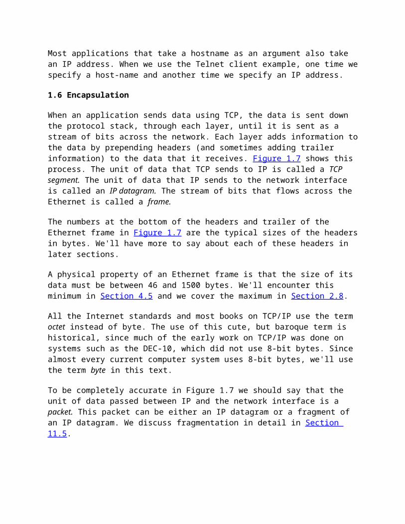
Figure 1.8 The demultiplexing of a received Ethernet frame.

Positioning the protocol boxes labeled "ICMP" and "IGMP" is always a challenge. In Figure 1.4 we showed them at the same layer as IP, because they really are adjuncts to IP. But here we show them above IP, to reiterate that ICMP messages and IGMP messages are encapsulated in IP datagrams.

We have a similar problem with the boxes "ARP" and "RARP." Here we show them above the Ethernet device driver because they both have their own Ethernet frame types, like IP datagrams. But in Figure 2.4 we'll show ARP as part of the Ethernet device driver, beneath IP, because that's where it logically fits.

Realize that these pictures of layered protocol boxes are not perfect.

When we describe TCP in detail we'll see that it really demultiplexes incoming segments using the destination port number, the source IP address, and the source port number.

1.8 Client-Server Model

Most networking applications are written assuming one side is the client and the other the server. The purpose of the application is for the server to provide some defined service for clients.

We can categorize servers into two classes: iterative or concurrent. An iterative server iterates through the following steps.

I1. Wait for a client request to arrive.

I2. Process the client request.

I3. Send the response back to the client that sent the request.

I4. Go back to step I1.

The problem with an iterative server is when step I2 takes a while. During this time no other clients are serviced. A concurrent server, on the other hand, performs the following steps.

Cl. Wait for a client request to arrive.

C2. Start a new server to handle this client's request. This may involve creating a new process, task, or thread, depending on what the underlying operating system supports. How this step is performed depends on the operating system.

This new server handles this client's entire request. When complete, this new server terminates.

C3. Go back to step Cl.

The advantage of a concurrent server is that the server just spawns other servers to handle the client requests. Each client has, in essence, its own server. Assuming the operating system allows multiprogramming, multiple clients are serviced concurrently.

The reason we categorize servers, and not clients, is because a client normally can't tell whether it's talking to an iterative server or a concurrent server.

As a general rule, TCP servers are concurrent, and UDP servers are iterative, but there are a few exceptions. We'll look in detail at the impact of UDP on its servers in Section 11.12, and the impact of TCP on its servers in Section 18.11.

1.9 Port Numbers

We said that TCP and UDP identify applications using 16-bit port numbers. How are these port numbers chosen?

Servers are normally known by their well-known port number. For example, every TCP/IP implementation that provides an FTP server provides that service on TCP port 21. Every Telnet server is on TCP port 23. Every implementation of TFTP (the Trivial File Transfer Protocol) is on UDP port 69. Those services that can be provided by any implementation of TCP/IP have well-known port numbers between 1 and 1023. The well-known ports are managed by the Internet Assigned Numbers Authority (IANA).

Until 1992 the well-known ports were between I and 255. Ports between 256 and 1023 were normally used by Unix systems for Unix-specific services-that is, services found on a

Unix system, but probably not found on other operating systems. The IANA now manages the ports between 1 and 1023.

An example of the difference between an Internet-wide service and a Unix-specific service is the difference between Telnet and Riogin. Both allow us to login across a network to another host. Telnet is a TCP/IP standard with a well-known port number of 23 and can be implemented on almost any operating system. Rlogin, on the other hand, was originally designed for Unix systems (although many non-Unix systems now provide it also) so its well-known port was chosen in the early 1980s as 513.

A client usually doesn't care what port number it uses on its end. All it needs to be certain of is that whatever port number it uses be unique on its host. Client port numbers are called ephemeral ports (i.e., short lived). This is because a client typically exists only as long as the user running the client needs its service, while servers typically run as long as the host is up.

Most TCP/IP implementations allocate ephemeral port numbers between 1024 and 5000. The port numbers above 5000 are intended for other servers (those that aren't well known across the Internet). We'll see many examples of how ephemeral ports are allocated in the examples throughout the text.

Solaris 2.2 is a notable exception. By default the ephemeral ports for TCP and UDP start at 32768. Section E.4 details the configuration options that can be modified by the system administrator to change these defaults.

The well-known port numbers are contained in the file /etc/services on most Unix systems. To find the port numbers for the Telnet server and the Domain Name System, we can execute

sun % grep telnet /etc/services telnet 23/tcp

says it uses TCP port 23

sun % grep domain /etc/servicesdomain 53/udpdomain 53/tcp

says it uses UDP port 53 and TCP port 53

Reserved Ports

Unix systems have the concept of reserved ports. Only a process with superuser privileges can assign itself a reserved port.

These port numbers are in the range of 1 to 1023, and are used by some applications (notably Rlogin, Section 26.2), as part of the authentication between the client and server.

1.10 Standardization Process

Who controls the TCP/IP protocol suite, approves new standards, and the like? There are four groups responsible for Internet technology.

1. The Internet Society (ISOC) is a professional society to facilitate, support, and promote the evolution and growth of the Internet as a global research communications infrastructure.

2. The Internet Architecture Board (IAB) is the technical oversight and coordination body. It is composed of about 15 international volunteers from various disciplines and serves as the final editorial and technical review board for the quality of Internet standards. The IAB falls under the ISOC.

3. The Internet Engineering Task Force (IETF) is the near-term, standards-oriented group, divided into nine areas (applications, routing and addressing, security, etc.). The IETF develops the specifications that become Internet standards. An additional Internet Engineering Steering Group (IESG) was formed to help the IETF chair.

4. The Internet Research Task Force (IRTF) pursues long-term research projects.

Both the IRTF and the IETF fall under the IAB. [Crocker 1993] provides additional details on the standardization process within the Internet, as well as some of its early history.

1.11 RFCs

All the official standards in the internet community are published as a Request for Comment, or RFC. Additionally there are lots of RFCs that are not official standards, but are published for informational purposes. The RFCs range in size from I page to almost 200 pages. Each is identified by a number, such as RFC 1122, with higher numbers for newer RFCs.

All the RFCs are available at no charge through electronic mail or using FTP across the Internet. Sending electronic mail as shown here:

To: rfc-info@OISI.EDU Subject: getting rfcs help: ways_to_get_rfcs

returns a detailed listing of various ways to obtain the RFCs.

The latest RFC index is always a starting point when looking for something. This index specifies when a certain RFC has been replaced by a newer RFC, and if a newer RFC updates some of the information in that RFC. There are a few important RFCs.

1. The Assigned Numbers RFC specifies all the magic numbers and constants that are used in the Internet protocols. At the time of this writing the latest version of this RFC is 1340 [Reynolds and Postel 1992]. All the Internet-wide well-known ports are listed here.

When this RFC is updated (it is normally updated at least yearly) the index listing for 1340 will indicate which RFC has replaced it.

2. The Internet Official Protocol Standards, currently RFC 1600 [Postel 1994]. This RFC specifies the state of standardization of the various Internet protocols. Each protocol has one of the following states of standardization: standard, draft standard, proposed standard, experimental, informational, or historic. Additionally each protocol has a requirement level: required, recommended, elective, limited use, or not recommended.

Like the Assigned Numbers RFC, this RFC is also reissued regularly. Be sure you're reading the current copy.

3. The Host Requirements RFCs, 1122 and 1123 [Braden 1989a, 1989b]. RFC 1122 handles the link layer, network layer, and transport layer, while RFC 1123 handles the application layer. These two RFCs make numerous corrections and interpretations of the important earlier RFCs, and are often the starting point when looking at any of the finer details of a given protocol. They list the features and implementation details of the protocols as either "must," "should," "may," "should not," or "must not."

[Borman 1993b] provides a practical look at these two RFCs, and RFC 1127 [Braden 1989c] provides an informal summary of the discussions and conclusions of the working group that developed the Host Requirements RFCs.

4. The Router Requirements RFC. The official version of this is RFC 1009 [Braden and Postel 1987], but a new version is nearing completion [Almquist 1993]. This is similar to the host requirements RFCs, but specifies the unique requirements of routers.

1.12 Standard, Simple Services

There are a few standard, simple services that almost every implementation provides. We'll use some of these servers throughout the text, usually with the Telnet client. Figure 1.9 describes these services. We can see from this figure that when the same service is provided using both TCP and UDP, both port numbers are normally chosen to be the same.

If we examine the port numbers for these standard services and other standard TCP/IP services (Telnet, FTP, SMTP, etc.), most are odd numbers. This is historical as these port numbers are derived from the NCP port numbers. (NCP, the Network Control Protocol, preceded TCP as a transport layer protocol for the ARPANET.) NCP was simplex, not full-duplex, so each application required two connections, and an even-odd pair of port numbers was reserved for each application. When TCP and UDP became the standard transport layers, only a single port number was needed per application, so the odd port numbers from NCP were used.

NameTCP port

UDP port

RFC Description

echo 7 7 862 Server returns whatever the client sends.

discard 9 9 863 Server discards whatever the client sends.

daytime 13 13 867Server returns the time and date in a human-readable format.

chargen 19 19 864

TCP server sends a continual stream of characters, until the connection is terminated by the client. UDP server sends a datagram containing a random number of characters each time the client sends a datagram.

time 37 37 868Server returns the time as a 32-bit binary number. This number represents the number of seconds since midnight January 1, 1900, UTC.

Figure 1.9 Standard, simple services provided by most implementations.

1.13 The Internet

In Figure 1.3 we showed an internet composed of two networks - an Ethernet and a token ring. In Sections 1.4 and 1.9 we talked about the worldwide Internet and the need to allocate IP addresses centrally (the InterNIC) and the well-known port numbers (the IANA). The word internet means different things depending on whether it's capitalized or not.

The lowercase internet means multiple networks connected together, using a common protocol suite. The uppercase Internet refers to the collection of hosts (over one million) around the world that can communicate with each other using TCP/IP. While the Internet is an internet, the reverse is not true.

1.14 Implementations

The de facto standard for TCP/IP implementations is the one from the Computer Systems Research Group at the University of California at Berkeley. Historically this has been distributed with the 4.x BSD system (Berkeley Software Distribution), and with the "BSD Networking Releases." This source code has been the starting point for many other implementations.

Figure 1.10 shows a chronology of the various BSD releases, indicating the important TCP/IP features. The BSD Networking Releases shown on the left side are publicly available source code releases containing all of the networking code: both the protocols themselves and many of the applications and utilities (such as Telnet and FTP).

Throughout the text we'll use the term Berkeley-derived implementation to refer to vendor implementations such as SunOS 4.x, SVR4, and AIX 3.2 that were originally developed from

the Berkeley sources. These implementations have much in common, often including the same bugs!

Figure 1.10 Various BSD releases with important TCP/IP features.

Much of the original research in the Internet is still being applied to the Berkeley system-new congestion control algorithms (Section 21.7), multicasting (Section 12.4), "long fat pipe" modifications (Section 24.3), and the like.

1.15 Application Programming Interfaces

Two popular application programming interfaces (APIs) for applications using the TCP/IP protocols are called sockets and TLI (Transport Layer Interface). The former is sometimes called "Berkeley sockets," indicating where it was originally developed. The latter, originally developed by AT&T, is sometimes called XTI (X/Open Transport Interface), recognizing the work done by X/Open, an international group of computer vendors that produce their own set of standards. XTI is effectively a superset of TLI.

This text is not a programming text, but occasional reference is made to features of TCP/IP that we look at, and whether that feature is provided by the most popular API (sockets) or not. All the programming details for both sockets and TLI are available in [Stevens 1990].

1.16 Test Network

Figure 1.11 shows the test network that is used for all the examples in the text. This figure is also duplicated on the inside front cover for easy reference while reading the book.

Figure 1.11 Test network used for all the examples in the text. All IP addresses begin with 140.252.

Most of the examples are run on the lower four systems in this figure (the author's subnet). All the IP addresses in this figure belong to the class B network ID 140.252. All the hostnames belong to the .tuc.noao.edu domain.(noao stands for "National Optical Astronomy Observatories" and tuc stands for Tucson.) For example, the lower right system has a complete hostname of svr4.tuc.noao.edu and an IP address of 140.252.13.34. The notation at the top of each box is the operating system running on that system. This collection of systems and networks provides hosts and routers running a variety of TCP/IP implementations.

It should be noted that there are many more networks and hosts in the noao.edu domain than we show in Figure 1.11. All we show here are the systems that we'll encounter throughout the text.

In Section 3.4 we describe the form of subnetting used on this network, and in Section 4.6 we'll provide more details on the dial-up SLIP connection between sun and netb. Section 2.4 describes SLIP in detail.

IP: Internet Protocol

3.1 Introduction

IP is the workhorse protocol of the TCP/IP protocol suite. All TCP, UDP, ICMP, and IGMP data gets transmitted as IP datagrams (Figure 1.4). A fact that amazes many newcomers to TCP/IP, especially those from an X.25 or SNA background, is that IP provides an unreliable, connectionless datagram delivery service.

By unreliable we mean there are no guarantees that an IP datagram successfully gets to its destination. IP provides a best effort service. When something goes wrong, such as a router temporarily running out of buffers, IP has a simple error handling algorithm: throw away the datagram and try to send an ICMP message back to the source. Any required reliability must be provided by the upper layers (e.g., TCP).

The term connectionless means that IP does not maintain any state information about successive datagrams. Each datagram is handled independently from all other datagrams. This also means that IP datagrams can get delivered out of order. If a source sends two consecutive datagrams (first A, then B) to the same destination, each is routed independently and can take different routes, with B arriving before A.

In this chapter we take a brief look at the fields in the IP header, describe IP routing, and cover subnetting. We also look at two useful commands: ifconfig and netstat. We leave a detailed discussion of some of the fields in the IP header for later when we can see exactly how the fields are used. RFC 791 [Postel 1981a] is the official specification of IP.

3.2 IP Header

Figure 3.1 shows the format of an IP datagram. The normal size of the IP header is 20 bytes, unless options are present.

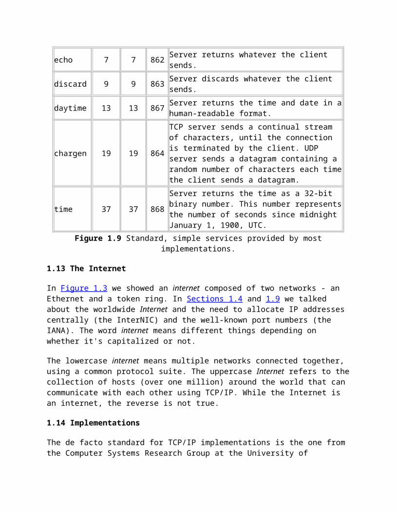
Figure 3.1 IP datagram, showing the fields in the IP header.

We will show the pictures of protocol headers in TCP/IP as in Figure 3.1. The most significant bit is numbered 0 at the left, and the least significant bit of a 32-bit value is numbered 31 on the right.

The 4 bytes in the 32-bit value are transmitted in the order: bits 0-7 first, then bits 8-15, then 16-23, and bits 24-31 last. This is called big endian byte ordering, which is the byte ordering required for all binary integers in the TCP/IP headers as they traverse a network. This is called the network byte order. Machines that store binary integers in other formats, such as the little endian format, must convert the header values into the network byte order before transmitting the data.

The current protocol version is 4, so IP is sometimes called IPv4. Section 3.10 discusses some proposals for a new version of IP.

The header length is the number of 32-bit words in the header, including any options. Since this is a 4-bit field, it limits the header to 60 bytes. In Chapter 8 we'll see that this limitation makes some of the options, such as the record route option, useless today. The normal value of this field (when no options are present) is 5.

The type-of-service field (TOS) is composed of a 3-bit precedence field (which is ignored today), 4 TOS bits, and an unused bit that must be 0. The 4 TOS bits are: minimize delay, maximize throughput, maximize reliability, and minimize monetary cost.

Only 1 of these 4 bits can be turned on. If all 4 bits are 0 it implies normal service. RFC 1340 [Reynolds and Postel 1992] specifies how these bits should be set by all the standard

applications. RFC 1349 [Almquist 1992] contains some corrections to this RFC, and a more detailed description of the TOS feature.

Figure 3.2 shows the recommended values of the TOS field for various applications. In the final column we show the hexadecimal value, since that's what we'll see in the tcpdump output later in the text.

ApplicationMinimize

delayMaximize

throughputMaximize reliability

Minimize monetary cost

Hex value

Telnet/Rlogin 1 0 0 0 0x10

FTP controldata

10

01

00

00

0x100x08

any bulk data 0 1 0 0 0x08

TFTP 1 0 0 0 0x10

SMTP command phasedata phase

10

01

00

00

0x100x08

DNS UDP queryTCP queryzone transfer

100

001

000

000

0x100x000x08

ICMPerrorquery

00

00

00

00

0x000x00

any IGP 0 0 1 0 0x04

SNMP 0 0 1 0 0x04

BOOTP 0 0 0 0 0x00

NNTP 0 0 0 1 0x02

Figure 3.2 Recommended values for type-of-service field.

The interactive login applications, Telnet and Rlogin, want a minimum delay since they're used interactively by a human for small amounts of data transfer. File transfer by FTP, on the other hand, wants maximum throughput. Maximum reliability is specified for network management (SNMP) and the routing protocols. Usenet news (NNTP) is the only one shown that wants to minimize monetary cost.

The TOS feature is not supported by most TCP/IP implementations today, though newer systems starting with 4.3BSD Reno are setting it. Additionally, new routing protocols such as OSPF and IS-IS are capable of making routing decisions based on this field.

In Section 2.10 we mentioned that SLIP drivers normally provide type-of-service queuing, allowing interactive traffic to be handled before bulk data. Since most implementations don't use the TOS field, this queuing is done ad hoc by SLIP, with the driver looking at the protocol field (to determine whether it's a TCP segment or not) and then checking the source and destination TCP port numbers to see if the port number corresponds to an interactive service. One driver comments that this "disgusting hack" is required since most implementations don't allow the application to set the TOS field.

The total length field is the total length of the IP datagram in bytes. Using this field and the header length field, we know where the data portion of the IP datagram starts, and its length. Since this is a 16-bit field, the maximum size of an IP datagram is 65535 bytes. (Recall from Figure 2.5 that a Hyperchannel has an MTU of 65535. This means there really isn't an MTU-it uses the largest IP datagram possible.) This field also changes when a datagram is fragmented, which we describe in Section 11.5.

Although it's possible to send a 65535-byte IP datagram, most link layers will fragment this. Furthermore, a host is not required to receive a datagram larger than 576 bytes. TCP divides the user's data into pieces, so this limit normally doesn't affect TCP. With UDP we'll encounter numerous applications in later chapters (RIP, TFTP, BOOTP, the DNS, and SNMP) that limit themselves to 512 bytes of user data, to stay below this 576-byte limit. Realistically, however, most implementations today (especially those that support the Network File System, NFS) allow for just over 8192-byte IP datagrams.

The total length field is required in the IP header since some data links (e.g., Ethernet) pad small frames to be a minimum length. Even though the minimum Ethernet frame size is 46 bytes (Figure 2.1), an IP datagram can be smaller. If the total length field wasn't provided, the IP layer wouldn't know how much of a 46-byte Ethernet frame was really an IP datagram.

The identification field uniquely identifies each datagram sent by a host. It normally increments by one each time a datagram is sent. We return to this field when we look at fragmentation and reassembly in Section 11.5. Similarly, we'll also look at the flags field and the fragmentation offset field when we talk about fragmentation.

RFC 791 [Postel 1981a] says that the identification field should be chosen by the upper layer that is having IP send the datagram. This implies that two consecutive IP datagrams, one generated by TCP and one generated by UDP, can have the same identification field. While this is OK (the reassembly algorithm handles this), most Berkeley-derived implementations have the IP layer increment a kernel variable each time an IP datagram is sent, regardless of which layer passed the data to IP to send. This kernel variable is initialized to a value based on the time-of-day when the system is bootstrapped.

The time-to-live field, or TTL, sets an upper limit on the number of routers through which a datagram can pass. It limits the lifetime of the datagram. It is initialized by the sender to some value (often 32 or 64) and decremented by one by every router that handles the datagram. When this field reaches 0, the datagram is thrown away, and the sender is

notified with an ICMP message. This prevents packets from getting caught in routing loops forever. We return to this field in Chapter 8 when we look at the Trace-route program.

We talked about the protocol field in Chapter 1 and showed how it is used by IP to demultiplex incoming datagrams in Figure 1.8. It identifies which protocol gave the data for IP to send.

The header checksum is calculated over the IP header only. It does not cover any data that follows the header. ICMP, IGMP, UDP, and TCP all have a checksum in their own headers to cover their header and data.

To compute the IP checksum for an outgoing datagram, the value of the checksum field is first set to 0. Then the 16-bit one's complement sum of the header is calculated (i.e., the entire header is considered a sequence of 16-bit words). The 16-bit one's complement of this sum is stored in the checksum field. When an IP datagram is received, the 16-bit one's complement sum of the header is calculated. Since the receiver's calculated checksum contains the checksum stored by the sender, the receiver's checksum is all one bits if nothing in the header was modified. If the result is not all one bits (a checksum error), IP discards the received datagram. No error message is generated. It is up to the higher layers to somehow detect the missing datagram and retransmit.

ICMP, IGMP, UDP, and TCP all use the same checksum algorithm, although TCP and UDP include various fields from the IP header, in addition to their own header and data. RFC 1071 [Braden, Borman, and Partridge 1988] contains implementation techniques for computing the Internet checksum. Since a router often changes only the TTL field (decrementing it by 1), a router can incrementally update the checksum when it forwards a received datagram, instead of calculating the checksum over the entire IP header again. RFC 1141 [Mallory and Kullberg 1990] describes an efficient way to do this.

The standard BSD implementation, however, does not use this incremental update feature when forwarding a datagram.

Every IP datagram contains the source IP address and the destination IP address. These are the 32-bit values that we described in Section 1.4.

The final field, the options, is a variable-length list of optional information for the datagram. The options currently defined are:

security and handling restrictions (for military applications, refer to RFC 1108 [Kent 1991] for details),

record route (have each router record its IP address. Section 7.3),

timestamp (have each router record its IP address and time. Section 7.4),

loose source routing (specifying a list of IP addresses that must be traversed by the datagram. Section 8.5), and

strict source routing (similar to loose source routing but here only the addresses in the list can be traversed. Section 8.5).

These options are rarely used and not all host and routers support all the options.

The options field always ends on a 32-bit boundary. Pad bytes with a value of 0 are added if necessary. This assures that the IP header is always a multiple of 32 bits (as required for the header length field).

3.3 IP Routing

Conceptually, IP routing is simple, especially for a host. If the destination is directly connected to the host (e.g., a point-to-point link) or on a shared network (e.g., Ethernet or token ring), then the IP datagram is sent directly to the destination. Otherwise the host sends the datagram to a default router, and lets the router deliver the datagram to its destination. This simple scheme handles most host configurations.

In this section and in Chapter 9 we'll look at the more general case where the IP layer can be configured to act as a router in addition to acting as a host. Most multiuser systems today, including almost every Unix system, can be configured to act as a router. We can then specify a single routing algorithm that both hosts and routers can use. The fundamental difference is that a host never forwards datagrams from one of its interfaces to another, while a router forwards datagrams. A host that contains embedded router functionality should never forward a datagram unless it has been specifically configured to do so. We say more about this configuration option in Section 9.4.

In our general scheme, IP can receive a datagram from TCP, UDP, ICMP, or IGMP (that is, a locally generated datagram) to send, or one that has been received from a network interface (a datagram to forward). The IP layer has a routing table in memory that it searches each time it receives a datagram to send. When a datagram is received from a network interface, IP first checks if the destination IP address is one of its own IP addresses or an IP broadcast address. If so, the datagram is delivered to the protocol module specified by the protocol field in the IP header. If the datagram is not destined for this IP layer, then (1) if the IP layer was configured to act as a router the packet is forwarded (that is, handled as an outgoing datagram as described below), else (2) the datagram is silently discarded.

Each entry in the routing table contains the following information:

Destination IP address. This can be either a complete host address or a network address, as specified by the flag field (described below) for this entry. A host address has a nonzero host ID (Figure 1.5) and identifies one particular host, while a network address has a host ID of 0 and identifies all the hosts on that network (e.g., Ethernet, token ring).

IP address of a next-hop router, or the IP address of a directly connected network. A next-hop router is one that is on a directly connected network to which we can send

datagrams for delivery. The next-hop router is not the final destination, but it takes the datagrams we send it and forwards them to the final destination.

Flags. One flag specifies whether the destination IP address is the address of a network or the address of a host. Another flag says whether the next-hop router field is really a next-hop router or a directly connected interface. (We describe each of these flags in Section 9.2.)

Specification of which network interface the datagram should be passed to for transmission.

IP routing is done on a hop-by-hop basis. As we can see from this routing table information, IP does not know the complete route to any destination (except, of course, those destinations that are directly connected to the sending host). All that IP routing provides is the IP address of the next-hop router to which the datagram is sent. It is assumed that the next-hop router is really "closer" to the destination than the sending host is, and that the next-hop router is directly connected to the sending host.

IP routing performs the following actions:

1. Search the routing table for an entry that matches the complete destination IP address (matching network ID and host ID). If found, send the packet to the indicated next-hop router or to the directly connected interface (depending on the flags field). Point-to-point links are found here, for example, since the other end of such a link is the other host's complete IP address.

2. Search the routing table for an entry that matches just the destination network ID. If found, send the packet to the indicated next-hop router or to the directly connected interface (depending on the flags field). All the hosts on the destination network can be handled with this single routing table entry All the hosts on a local Ethernet, for example, are handled with a routing table entry of this type.

This check for a network match must take into account a possible subnet mask, which we describe in the next section.

3. Search the routing table for an entry labeled "default." If found, send the packet to the indicated next-hop router.

If none of the steps works, the datagram is undeliverable. If the undeliverable datagram was generated on this host, a "host unreachable" or "network unreachable" error is normally returned to the application that generated the datagram.

A complete matching host address is searched for before a matching network ID. Only if both of these fail is a default route used. Default routes, along with the ICMP redirect message sent by a next-hop router (if we chose the wrong default for a datagram), are powerful features of IP routing that we'll come back to in Chapter 9.

The ability to specify a route to a network, and not have to specify a route to every host, is another fundamental feature of IP routing. Doing this allows the routers on the Internet, for example, to have a routing table with thousands of entries, instead of a routing table with more than one million entries.

Examples

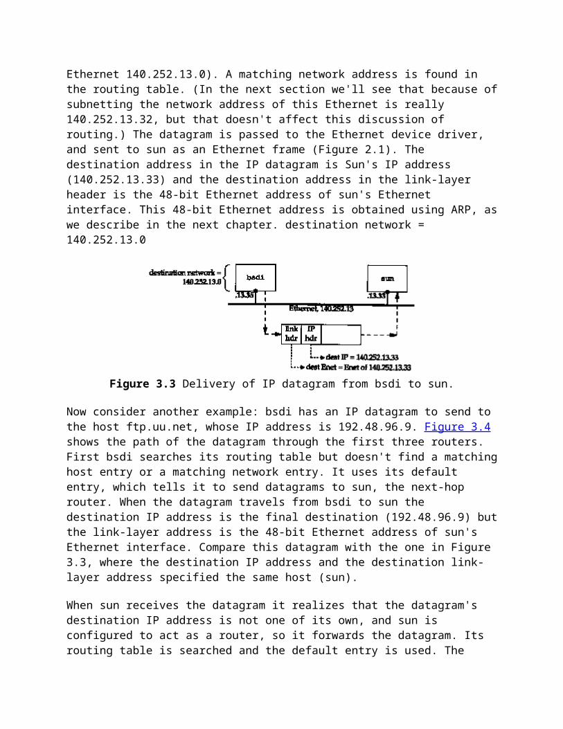
First consider a simple example: our host bsdi has an IP datagram to send to our host sun. Both hosts are on the same Ethernet (see inside front cover). Figure 3.3 shows the delivery of the datagram.

When IP receives the datagram from one of the upper layers it searches its routing table and finds that the destination IP address (140.252.13.33) is on a directly connected network (the Ethernet 140.252.13.0). A matching network address is found in the routing table. (In the next section we'll see that because of subnetting the network address of this Ethernet is really 140.252.13.32, but that doesn't affect this discussion of routing.) The datagram is passed to the Ethernet device driver, and sent to sun as an Ethernet frame (Figure 2.1). The destination address in the IP datagram is Sun's IP address (140.252.13.33) and the destination address in the link-layer header is the 48-bit Ethernet address of sun's Ethernet interface. This 48-bit Ethernet address is obtained using ARP, as we describe in the next chapter. destination network = 140.252.13.0

Figure 3.3 Delivery of IP datagram from bsdi to sun.

Now consider another example: bsdi has an IP datagram to send to the host ftp.uu.net, whose IP address is 192.48.96.9. Figure 3.4 shows the path of the datagram through the first three routers. First bsdi searches its routing table but doesn't find a matching host entry or a matching network entry. It uses its default entry, which tells it to send datagrams to sun, the next-hop router. When the datagram travels from bsdi to sun the destination IP address is the final destination (192.48.96.9) but the link-layer address is the 48-bit Ethernet address of sun's Ethernet interface. Compare this datagram with the one in Figure 3.3, where the destination IP address and the destination link-layer address specified the same host (sun).

When sun receives the datagram it realizes that the datagram's destination IP address is not one of its own, and sun is configured to act as a router, so it forwards the datagram. Its routing table is searched and the default entry is used. The default entry on sun tells it to

send datagrams to the next-hop router netb, whose IP address is 140.252.1.183. The datagram is sent across the point-to-point SLIP link, using the minimal encapsulation we showed in Figure 2.2. We don't show a link-layer header, as we do on the Ethernets, because there isn't one on a SLIP link.

When netb receives the datagram it goes through the same steps that sun just did: the datagram is not destined for one of its own IP addresses, and netb is configured to act as a router, so the datagram is forwarded. The default routing table entry is used, sending the datagram to the next-hop router gateway (140.252.1.4). ARP is used by netb on the Ethernet 140.252.1 to obtain the 48-bit Ethernet address corresponding to 140.252.1.4, and that Ethernet address is the destination address in the link-layer header.

gateway goes through the same steps as the previous two routers and its default routing table entry specifies 140.252.104.2 as the next-hop router. (We'll verify that this is the next-hop router for gateway using Traceroute in Figure 8.4.)

Figure 3.4 Initial path of datagram from bsdi to ftp.uu.net (192.48.96.9).

A few key points come out in this example.

1. All the hosts and routers in this example used a default route. Indeed, most hosts and some routers can use a default route for everything other than destinations on local networks.

2. The destination IP address in the datagram never changes. (In Section 8.5 we'll see that this is not true only if source routing is used, which is rare.) All the routing decisions are based on this destination address.

3. A different link-layer header can be used on each link, and the link-layer destination address (if present) always contains the link-layer address of the next hop. In our example both Ethernets encapsulated a link-layer header containing the next-hop's Ethernet address, but the SLIP link did not. The Ethernet addresses are normally obtained using ARP.

In Chapter 9 we'll look at IP routing again, after describing ICMP. We'll also look at some sample routing tables and how they're used for routing decisions.

3.4 Subnet Addressing

All hosts are now required to support subnet addressing (RFC 950 [Mogul and Postel 1985]). Instead of considering an IP address as just a network ID and host ID, the host ID portion is divided into a subnet ID and a host ID.

This makes sense because class A and class B addresses have too many bits allocated for the host ID: 224-2 and 216-2, respectively. People don't attach that many hosts to a single network. (Figure 1.5 shows the format of the different classes of IP addresses.) We subtract 2 in these expressions because host IDs of all zero bits or all one bits are invalid.

After obtaining an IP network ID of a certain class from the InterNIC, it is up to the local system administrator whether to subnet or not, and if so, how many bits to allocate to the subnet ID and host ID. For example, the internet used in this text has a class B network address (140.252) and of the remaining 16 bits, 8 are for the subnet ID and 8 for the host ID. This is shown in Figure 3.5.

16 bits 8 bits 8 bitsClass B netid = 140.252 subnetid hostid

Figure 3.5 Subnetting a class B address.

This division allows 254 subnets, with 254 hosts per subnet.

Many administrators use the natural 8-bit boundary in the 16 bits of a class B host ID as the subnet boundary. This makes it easier to determine the subnet ID from a dotted-decimal number, but there is no requirement that the subnet boundary for a class A or class B address be on a byte boundary.

Most examples of subnetting describe it using a class B address. Subnetting is also allowed for a class C address, but there are fewer bits to work with. Subnetting is rarely shown with

a class A address because there are so few class A addresses. (Most class A addresses are, however, subnetted.)

Subnetting hides the details of internal network organization (within a company or campus) to external routers. Using our example network, all IP addresses have the class B network ID of 140.252. But there are more than 30 subnets and more than 400 hosts distributed over those subnets. A single router provides the connection to the Internet, as shown in Figure 3.6.

In this figure we have labeled most of the routers as Rn, where n is the subnet number. We show the routers that connect these subnets, along with the nine systems from the figure on the inside front cover. The Ethernets are shown as thicker lines, and the point-to-point links as dashed lines. We do not show all the hosts on the various subnets. For example, there are more than 50 hosts on the 140.252.3 subnet, and more than 100 on the 140.252.1 subnet.

The advantage to using a single class B address with 30 subnets, compared to 30 class C addresses, is that subnetting reduces the size of the Internet's routing tables. The fact that the class B address 140.252 is subnetted is transparent to all Internet routers other than the ones within the 140.252 subnet. To reach any host whose IP

Figure 3.6 Arrangement of most of the noao.edu 140.252 subnets.

address begins with 140.252, the external routers only need to know the path to the IP address 140.252.104.1. This means that only one routing table entry is needed for all the 140.252 networks, instead of 30 entries if 30 class C addresses were used. Subnetting, therefore, reduces the size of routing tables. (In Section 10.8 we'll look at a new technique that helps reduce the size of routing tables even if class C addresses are used.)

To show that subnetting is not transparent to routers within the subnet, assume in Figure 3.6 that a datagram arrives at gateway from the Internet with a destination address of 140.252.57.1. The router gateway needs to know that the subnet number is 57, and that datagrams for this subnet are sent to kpno. Similarly kpno must send the datagram to R55, who then sends it to R57.

3.5 Subnet Mask

Part of the configuration of any host that takes place at bootstrap time is the specification of the host's IP address. Most systems have this stored in a disk file that's read at bootstrap time, and we'll see in Chapter 5 how a diskless system can also find out its IP address when it's bootstrapped.

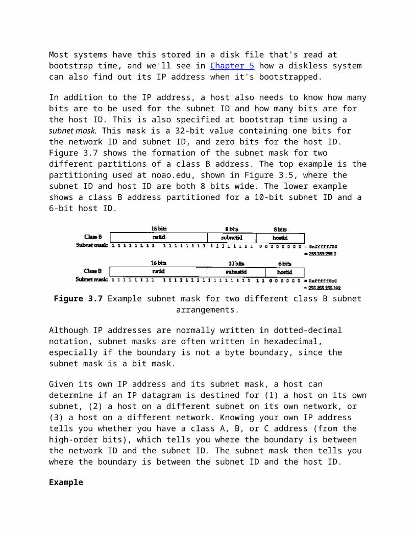
In addition to the IP address, a host also needs to know how many bits are to be used for the subnet ID and how many bits are for the host ID. This is also specified at bootstrap time using a subnet mask. This mask is a 32-bit value containing one bits for the network ID and subnet ID, and zero bits for the host ID. Figure 3.7 shows the formation of the subnet mask for two different partitions of a class B address. The top example is the partitioning used at noao.edu, shown in Figure 3.5, where the subnet ID and host ID are both 8 bits wide. The lower example shows a class B address partitioned for a 10-bit subnet ID and a 6-bit host ID.

Figure 3.7 Example subnet mask for two different class B subnet arrangements.

Although IP addresses are normally written in dotted-decimal notation, subnet masks are often written in hexadecimal, especially if the boundary is not a byte boundary, since the subnet mask is a bit mask.

Given its own IP address and its subnet mask, a host can determine if an IP datagram is destined for (1) a host on its own subnet, (2) a host on a different subnet on its own network, or (3) a host on a different network. Knowing your own IP address tells you whether you have a class A, B, or C address (from the high-order bits), which tells you

where the boundary is between the network ID and the subnet ID. The subnet mask then tells you where the boundary is between the subnet ID and the host ID.

Example

Assume our host address is 140.252.1.1 (a class B address) and our subnet mask is 255.255.255.0 (8 bits for the subnet ID and 8 bits for the host ID).

If a destination IP address is 140.252.4.5, we know that the class B network IDs are the same (140.252), but the subnet IDs are different (1 and 4). Figure 3.8 shows how this comparison of two IP addresses is done, using the subnet mask.

If the destination IP address is 140.252.1.22, the class B network IDs are the same (140.252), and the subnet IDs are the same (1). The host IDs, however, are different.

If the destination IP address is 192.43.235.6 (a class C address), the network IDs are different. No further comparisons can be made against this address.

Figure 3.8 Comparison of two class B addresses using a subnet mask.

The IP routing function makes comparisons like this all the time, given two IP addresses and a subnet mask.

3.6 Special Case IP Addresses

Having described subnetting we now show the seven special case IP addresses in Figure 3.9. In this figure, 0 means a field of all zero bits, -1 means a field of all one bits, and netid, subnetid, and hostid mean the corresponding field that is neither all zero bits nor all one bits. A blank subnet ID column means the address is not subnetted.

IP address Can appear as Description

net IDsubnet

IDhost ID source? destination?

0 0

0hostid

OKOK

nevernever

this host on this net (see restrictions below)specified host on this net (see restrictions below)

127 anything OK OK loopback address

-1 netidnetidnetid

subnetid1

-1 -1-1-1

nevernevernevernever

OKOKOKOK

limited broadcast (never forwarded)net-directed broadcast to netidsubnet-directed broadcast to netid, subnetidall-subnets-directed broadcast to netid

Figure 3.9 Special case IP addresses.

We have divided this table into three sections. The first two entries are special case source addresses, the next one is the special loopback address, and the final four are the broadcast addresses.

"The first two entries in the table, with a network ID of 0, can only appear as the source address as part of an initialization procedure when a host is determining its own IP address, for example, when the BOOTP protocol is being used (Chapter 16). In Section 12.2 we'll examine the four types of broadcast addresses in more detail.

3.7 A Subnet Example

This example shows the subnet used in the text, and how two different subnet masks are used. Figure 3.10 shows the arrangement.

Figure 3.10 Arrangement of hosts and networks for author's subnet.

If you compare this figure with the one on the inside front cover, you'll notice that we've omitted the detail that the connection from the router sun to the top Ethernet in Figure 3.10 is really a dialup SLIP connection. This detail doesn't affect our description of subnetting in this section. We'll return to this detail in Section 4.6 when we describe proxy ARP.

The problem is that we have two separate networks within subnet 13: an Ethernet and a point-to-point link (the hardwired SLIP link). (Point-to-point links always cause problems

since each end normally requires an IP address.) There could be more hosts and networks in the future, but not enough hosts across the different networks to justify using another subnet number. Our solution is to extend the subnet ID from 8 to II bits, and decrease the host ID from 8 to 5 bits. This is called variable-length subnets since most networks within the 140.252 network use an 8-bit subnet mask while our network uses an 11-bit subnet mask.

RFC 1009 [Braden and Postel 1987] allows a subnetted network to use more than one subnet mask. The new Router Requirements RFC [Almquist 1993] requires support for this.

The problem, however, is that not all routing protocols exchange the subnet mask along with the destination network ID. We'll see in Chapter 10 that RIP does not support variable-length subnets, while RIP Version 2 and OSPF do. We don't have a problem with our example, since RIP isn't required on the author's subnet.

Figure 3.11 shows the IP address structure used within the author's subnet. The first 8 bits of the 11-bit subnet ID are always 13 within the author's subnet. For the remaining 3 bits of the subnet ID, we use binary 001 for the Ethernet, and binary 010 for

Figure 3.11 Using variable-length subnets.

the point-to-point SLIP link. This variable-length subnet mask does not cause a problem for other hosts and routers in the 140.252 network-as long as all datagrams destined for the subnet 140.252.13 are sent to the router sun (IP address 140.252.1.29) in Figure 3.10, and if sun knows about the 11-bit subnet ID for the hosts on its subnet 13, everything is fine.

The subnet mask for all the interfaces on the 140.252.13 subnet is 255.255.255.224, or 0xffffffe0. This indicates that the rightmost 5 bits are for the host ID, and the 27 bits to the left are the network ID and subnet ID.

Figure 3.12 shows the allocation of IP addresses and subnet masks for the interfaces shown in Figure 3.10.

Host IP address Subnet maskNet ID/Subnet

IDHost

IDComment

sun140.252.1.29 140.252.13.33

255.255.255.0 255.255.255.224

140.252.1 140.252.13.32

29 1

on subnet 1on author's Ethernet

svr4 140.252.13.34 255.255.255.224 140.252.13.32 2

bsdi140.252.13.35 140.252.13.66

255.255.255.224 255.255.255.224

140.252.13.32 140.252.13.64

3 2

on Ethernetpoint-to-point

slip 140.252.13.65 255.255.255.224 140.252.13.64 1 point-to-point

140.252.13.63 255.255.255.224 140.252.13.32 31broadcast addr on Ethernet

Figure 3.12 IP addresses on author's subnet.

The first column is labeled "Host," but both sun and bsdi also act as routers, since they are multihomed and route packets from one interface to another.

The final row in this table notes that the broadcast address for the Ethernet in Figure 3.10 is 140.252.13.63: it is formed from the subnet ID of the Ethernet (140.252.13.32) and the low-order 5 bits in Figure 3.11 set to 1 (16+8+4+2+1 = 31). (We'll see in Chapter 12 that this address is called the subnet-directed broadcast address.)

3.8 ifconfig Command

Now that we've described the link layer and the IP layer we can show the command used to configure or query a network interface for use by TCP/IP. The ifconfig(8) command is normally run at bootstrap time to configure each interface on a host.

For dialup interfaces that may go up and down (such as SLIP links), ifconfig must be run (somehow) each time the line is brought up or down. How this is done each time the SLIP link is brought up or down depends on the SLIP software being used.

The following output shows the values for the author's subnet. Compare these values with the values in Figure 3.12.

sun % /usr/etc/ifconfig -a SunOS -a option says report on all interfaces leO : flags=63<UP, BROADCAST, NOTRAILERS, RUNNING> inet 140.252.13.33 netmask ffffffe0 broadcast 140.252.13.63 slO : flags=105KUP, POINTOPOINT, RUNNING, LINKO>inet 140.252.1.29 -> 140.252.1.183 netmask ffffff00 loO: flags=49<UP,LOOPBACK,RUNNING>inet 127.0.0.1 netmask ff000000

The loopback interface (Section 2.7) is considered a network interface. Its class A address is not subnetted.

Other things to notice are that trailer encapsulation (Section 2.3) is not used on the Ethernet, and that the Ethernet is capable of broadcasting, while the SLIP link is a point-to-point link.

The flag LINK0 for the SLIP interface is the configuration option that enables compressed slip (CSLIP, Section 2.5). Other possible options are LINK1, which enables CSLIP if a compressed packet is received from the other end, and LINK2, which causes all outgoing ICMP packets to be thrown away. We'll look at the destination address of this SLIP link in Section 4.6.

A comment in the installation instructions gives the reason for this last option: "This shouldn't have to be set, but some cretin pinging you can drive your throughput to zero."

bsdi is the other router. Since the -a option is a SunOS feature, we have to execute ifconfig multiple times, specifying the interface name as an argument:

bsdi % /sbin/ifconfig weO we0: flags=863<UP, BROADCAST, NOTRAILERS, RUNNING, SIMPLEX> inet 140.252.13.35 netmask ffffffe0 broadcast 140.252.13.63 bsdi % /sbin/ifconfig slO sl0 : flags=1011<UP, POINTOPOINT, LINKO inet 140.252.13.66 -> 140.252.13.65 netmask ffffffe0

Here we see a new option for the Ethernet interface (we0): SIMPLEX. This 4.4BSD flag specifies that the interface can't hear its own transmissions. It is set in BSD/386 for all the Ethernet interfaces. When set, if the interface is sending a frame to the broadcast address, a copy is made for the local host and sent to the loopback address. (We show an example of this feature in Section 6.3.)

On the host slip the configuration of the SLIP interface is nearly identical to the output shown above on bsdi, with the exception that the IP addresses of the two ends are swapped:

slip % /sbin/ifconfig slO sl0 : flags=1011<UP, POINTOPOINT, LINK0 inet 140.252.13.65 --> 140.252.13.66 netmask ffffffe0

The final interface is the Ethernet interface on the host svr4. It is similar to the Ethernet output shown earlier, except that SVR4's version of ifconfig doesn't print the RUNNING flag:

svr4 % /usr/sbin/ifconfig emdO emdO: flags=23<UP, BROADCAST, NOTRAILERS> inet 140.252.13.34 netmask ffffffe0 broadcast 140.252.13.63

The ifconfig command normally supports other protocol families (other than TCP/IP) and has numerous additional options. Check your system's manual for these details.

3.9 netstat Command

The netstat(l) command also provides information about the interfaces on a system. The -i flag prints the interface information, and the -n flag prints IP addresses instead of hostnames.

sun % netstat -in Name Mtu Net/Dest Address lpkts lerrs Opkts Oerrs Collis Queue leO 1500 140.252.13.32 140.252.13.33 67719 0 92133 0 1 0 slO 552 140.252.1.183 140.252.1.29 48035 0 54963 0 0 0 loO 1536 127.0.0.0 127.0.0.1 15548 0 15548 0 0 0

This command prints the MTU of each interface, the number of input packets, input errors, output packets, output errors, collisions, and the current size of the output queue.

We'll return to the netstat command in Chapter 9 when we use it to examine the routing table, and in Chapter 13 when we use a modified version to see active multicast groups.

3.10 IP Futures

There are three problems with IP. They are a result of the phenomenal growth of the Internet over the past few years. (See Exercise 1.2 also.)

1. Over half of all class B addresses have already been allocated. Current estimates predict exhaustion of the class B address space around 1995, if they continue to be allocated as they have been in the past.

2. 32-bit IP addresses in general are inadequate for the predicted long-term growth of the Internet.

3. The current routing structure is not hierarchical, but flat, requiring one routing table entry per network. As the number of networks grows, amplified by the allocation of multiple class C addresses to a site with multiple networks, instead of a single class B address, the size of the routing tables grows.

CIDR (Classless Interdomain Routing) proposes a fix to the third problem that will extend the usefulness of the current version of IP (IP version 4) into the next century. We discuss it in more detail in Section 10.8.

Four proposals have been made for a new version of IP, often called IPng, for the next generation of IP. The May 1993 issue of IEEE Network (vol. 7, no. 3) contains overviews of the first three proposals, along with an article on CIDR. RFC 1454 [Dixon 1993] also compares the first three proposals.

1. SIP, the Simple Internet Protocol. It proposes a minimal set of changes to IP that uses 64-bit addresses and a different header format. (The first 4 bits of the header still contain the version number, with a value other than 4.)

2. PIP. This proposal also uses larger, variable-length, hierarchical addresses with a different header format.

3. TUBA, which stands for "TCP and UDP with Bigger Addresses," is based on the OSI CLNP (Connectionless Network Protocol), an OSI protocol similar to IP. It provides much larger addresses: variable length, up to 20 bytes. Since CLNP is an existing protocol, whereas SIP and PIP are just proposals, documentation already exists on CLNP. RFC 1347 [Gallon 1992] provides details on TUBA. Chapter 7 of [Periman 1992] contains a comparison of IPv4 and CLNP. Many routers already support CLNP, but few hosts do.

4. TP/IX, which is described in RFC 1475 [Ullmann 1993]. As with SIP, it uses 64 bits for IP addresses, but it also changes the TCP and UDP headers: 32-bit port number for both protocols, along with 64-bit sequence numbers, 64-bit acknowledgment numbers, and 32-bit windows for TCP.

The first three proposals use basically the same versions of TCP and UDP as the transport layers.

Since only one of these four proposals will be chosen as the successor to IPv4, and since the decision may have been made by the time you read this, we won't say any more about them. With the forthcoming implementation of CIDR to handle the short-term problem, it will take many years to implement the successor to IPv4.

UNIT-II

ICMP: Internet Control Message Protocol

6.1 Introduction

ICMP is often considered part of the IP layer. It communicates error messages and other conditions that require attention. ICMP messages are usually acted on by either the IP layer or the higher layer protocol (TCP or UDP). Some ICMP messages cause errors to be returned to user processes.

ICMP messages are transmitted within IP datagrams, as shown in Figure 6.1.

Figure 6.1 ICMP messages encapsulated within an IP datagram.

RFC 792 [Postel 1981b] contains the official specification of ICMP.

Figure 6.2 shows the format of an ICMP message. The first 4 bytes have the same format for all messages, but the remainder differs from one message to the next. We'll show the exact format of each message when we describe it.

There are 15 different values for the type field, which identify the particular ICMP message. Some types of ICMP messages then use different values of the code field to further specify the condition.

The checksum field covers the entire ICMP message. The algorithm used is the same as we described for the IP header checksum in Section 3.2. The ICMP checksum is required.

Figure 6.2 ICMP message.

In this chapter we talk about ICMP messages in general and a few in detail: address mask request and reply, timestamp request and reply, and port unreachable. We discuss the echo request and reply messages in detail with the Ping program in Chapter 7, and we discuss the ICMP messages dealing with IP routing in Chapter 9.

6.2 ICMP Message Types

Figure 6.3 lists the different ICMP message types, as determined by the type field and code field in the ICMP message.

The final two columns in this figure specify whether the ICMP message is a query message or an error message. We need to make this distinction because ICMP error messages are sometimes handled specially. For example, an ICMP error message is never generated in response to an ICMP error message. (If this were not the rule, we could end up with scenarios where an error generates an error, which generates an error, and so on, indefinitely)

When an ICMP error message is sent, the message always contains the IP header and the first 8 bytes of the IP datagram that caused the ICMP error to be generated. This lets the receiving ICMP module associate the message with one particular protocol (TCP or UDP from the protocol field in the IP header) and one particular user process (from the TCP or UDP port numbers that are in the TCP or UDP header contained in the first 8 bytes of the IP datagram). We'll show an example of this in Section 6.5. An ICMP error message is never generated in response to

1. An ICMP error message. (An ICMP error message may, however, be generated in response to an ICMP query message.)

2. A datagram destined to an IP broadcast address (Figure 3.9) or an IP multicast address (a class D address, Figure 1.5).

3. A datagram sent as a link-layer broadcast.

4. A fragment other than the first. (We describe fragmentation in Section 11.5.)

5. A datagram whose source address does not define a single host. This means the source address cannot be a zero address, a loopback address, a broadcast address, or a multicast address.

type code Description Query Error

0 0 echo reply (Ping reply. Chapter 7) *

30123456789

10

destination unreachable:network unreachable (Section 9.3)host unreachable (Section 9.3)protocol unreachableport unreachable (Section 6.5)fragmentation needed but don't-fragment bit set (Section 11.6)source route failed (Section 8.5)destination network unknowndestination host unknownsource host isolated (obsolete)destination network administratively prohibited

***********

1112131415

destination host administratively prohibitednetwork unreachable for TOS (Section 9.3)host unreachable for TOS (Section 9.3)communication administratively prohibited by filteringhost precedence violationprecedence cutoff in effect

*****

4 0 source quench (elementary flow control. Section 11.11) *

50123

redirect (Section 9.5): redirect for networkredirect for hostredirect for type-of-service and networkredirect for type-of-service and host

****

8 0 echo request (Ping request. Chapter 7) *

9 10

00

router advertisement (Section 9.6) router solicitation (Section 9.6)

**

11 01

time exceeded:time-to-live equals 0 during transit (Traceroute, Chapter 8)time-to-live equals 0 during reassembly (Section 11.5)

**

12 01

parameter problem:IP header bad (catchall error)required option missing

**

1314

00

timestamp request (Section 6.4)timestamp reply (Section 6.4)

**

1516

00

information request (obsolete)information reply (obsolete)

**

1718

00

address mask request (Section 6.3)address mask reply (Section 6.3)

**

Figure 6.3 ICMP message types.

These rules are meant to prevent the broadcast storms that have occurred in the past when ICMP errors were sent in response to broadcast packets.

6.3 ICMP Address Mask Request and Reply

The ICMP address mask request is intended for a diskless system to obtain its subnet mask (Section 3.5) at bootstrap time. The requesting system broadcasts its ICMP request. (This is similar to a diskless system using RARP to obtain its IP address at bootstrap time.) An alternative method for a diskless system to obtain its subnet mask is the BOOTP protocol, which we describe in Chapter 16. Figure 6.4 shows the format of the ICMP address mask request and reply messages.

Figure 6.4 ICMP address mask request and reply messages.

The identifier and sequence number fields in the ICMP message can be set to anything the sender chooses, and these values are returned in the reply This allows the sender to match replies with requests.

We can write a simple program (named icmpaddrmask) that issues an ICMP address mask request and prints all replies. Since normal usage is to send the request to the broadcast address, that's what we'll do. The destination address (140.252.13.63) is the broadcast address for the subnet 140.252.13.32 (Figure 3.12).

sun % icmpaddnnask 140.252.13.63received mask = ffffffeO, from 140.252.13.33received mask = ffffffeO, from 140.252.13.35received mask = ffff0000, from 140.252.13.34

from ourselffrom bsdifrom svr4

The first thing we note in this output is that the returned value from svr4 is wrong. It appears that SVR4 is returning the general class B address mask, assuming no subnets, even though the interface on svr4 has been configured with the correct subnet mask:

svr4 % ifconfig emd0 emd0: flags=23<UP, BROADCAST ,NOTRAILERS>inet 140.252.13.34 netmask ffffffe0 broadcast 140.252.13.63

There is a bug in the SVR4 handling of the ICMP address mask request.

We'll watch this exchange on the host bsdi using tcpdump. The output is shown in Figure 6.5. We specify the -e option to see the hardware addresses.

1 0.0 8:0:20:3:f6:42 ff;ff:ff:ff:ff:ff ip 60: sun > 140.252.13.63: icmp: address mask request

2 0.00 (0.00) 0:0:c0:6f:2d:40 ff;ff:ff:ff:ff:ff ip 46: bsdi > sun: icmp: address mask is 0xffffffe0

3 0.01 (0.01) 0:0:c0:c2:9b:26 8:0:20:3:f6:42 ip 60: svr4 > sun: icmp: address mask is 0xffff0000

Figure 6.5 ICMP address mask request sent to broadcast address.

Note that the sending host, sun, receives an ICMP reply (the output line with the comment from ourself shown earlier), even though nothing is seen on the wire. This is a general characteristic of broadcasting: the sending host receives a copy of the broadcast packet through some internal loopback mechanism. Since by definition the term "broadcast" means all the hosts on the local network, it should include the sending host. (Referring to Figure 2.4 what is happening is that when the Ethernet driver recognizes that the destination address is the broadcast address, the packet is sent onto the network and a copy is made and passed to the loopback interface.)

Next, bsdi broadcasts the reply, while svr4 sends the reply only to the requestor. Normally the reply should be unicast unless the source IP address of the request is 0.0.0.0, which it isn't in this example. Therefore, sending the reply to the broadcast address is a BSD/386 bug.

The Host Requirements RFC says that a system must not send an address mask reply unless it is an authoritative agent for address masks. (To be an authoritative agent it must be specifically configured to send these replies. See Appendix E.) As we can see from this example, however, most host implementations send a reply if they get a request. Some hosts even send the wrong reply!

The final point is shown by the following example. We send an address mask request to our own IP address and to the loopback address:

sun % icmpaddrmask sun received mask = ff000000, from 140.252.13.33 sun % icmpaddrmask localhostreceived mask = ff000000, from 127.0.0.1

In both cases the returned address mask corresponds to the loopback address, the class A address 127.0.0.1. Again, referring to Figure 2.4 we see that IP datagrams sent to the host's own IP address (140.252.13.33 in this example) are actually sent to the loop-back interface. The ICMP address mask reply must correspond to the subnet mask of the interface on which the request was received (since a multihomed host can have different subnet masks for each interface), and in both cases the request is received from the loopback interface.

6.4 ICMP Timestamp Request and Reply

The ICMP timestamp request allows a system to query another for the current time. The recommended value to be returned is the number of milliseconds since midnight, Coordinated Universal Time (UTC). (Older manuals refer to UTC as Greenwich Mean Time.) The nice feature of this ICMP message is that it provides millisecond resolution, whereas some other methods for obtaining the time from another host (such as the rdate command provided by some Unix systems) provide a resolution of seconds. The drawback is that only the time since midnight is returned-the caller must know the date from some other means. Figure 6.6 shows the format of the ICMP timestamp request and reply messages.

Figure 6.6 ICMP timestamp request and reply messages.

The requestor fills in the originate timestamp and sends the request. The replying system fills in the receive timestamp when it receives the request, and the transmit time-stamp when it sends the reply. In actuality, however, most implementations set the latter two fields to the same value. (The reason for providing the three fields is to let the sender compute the time for the request to be sent, and separately compute the time for the reply to be sent.)

We can write a simple program (named icmptime) that sends an ICMP timestamp request to a host and prints the returned reply. We try it first on our small internet:

sun % icmptime bsdi orig = 83573336, recv = 83573330, xmit = 83573330, rtt = 2 msdifference = -6 ms sun % icmptime bsdi orig = 83577987, recv = 83577980, xmit = 83577980, rtt = 2 msdifference = -7 ms

The program prints the three timestamps in the ICMP message: the originate (orig), receive (recv), and transmit (xmit) timestamps. As we can see in this and the following examples, all the hosts set the receive and transmit timestamps to the same value.

We also calculate the round-trip time (rtt), which is the time the reply is received minus the time the request was sent. The difference is the received timestamp minus the originate timestamp. Figure 6.7 shows the relationship between these values.

Figure 6.7 Relationship between values printed by our icmptime program.

If we believe the RTT and assume that one-half of the RTT is for the request, and the other half for the reply, then the sender's clock needs to be adjusted by difference minus one-half the RTT, to have the same time as the host being queried. In the preceding example, the clock on bsdi was 7 and 8 ms behind the clock on sun.

Since the timestamp values are the number of milliseconds past midnight, UTC, they should always be less than 86,400,000 (24 x 60 x 60 x 1000). These examples were run just before 4:00 P.M. in a time zone that is 7 hours behind UTC, so the values being greater than 82,800,000 (2300 hours) makes sense.

If we run this program several times to the host bsdi we see that the final digit in the receive and transmit timestamp is always 0. This is because the software release (Version 0.9.4) only provides a 10-ms clock. (We describe this in Appendix B.)

If we run the program twice to the host svr4 we see that the low-order three digits of the SVR4 timestamp are always 0:

sun % icmptime svr4orig = 83588210, recv = 83588000, xmit = 83588000, rtt = 4 msdifference = -210 ms sun % icmptime svr4 orig = 83591547, recv = 83591000, xmit = 83591000, rtt = 4 msdifference = -547 ms

For some reason SVR4 doesn't provide any millisecond resolution using the ICMP time-stamp. This imprecision makes the calculated differences useless for subsecond adjustments.

If we try two other hosts on the 140.252.1 subnet, the results show that one clock differs from sun's by 3.7 seconds, and the other by nearly 75 seconds:

sun % icmptime gemini orig = 83601883, recv = 83598140, xmit = 83598140, rtt = 247 msdifference = -3743 ms sun % icmptime aix orig = 83606768, recv = 83532183, xmit = 83532183, rtt = 253 msdifference = -74585 ms

Another interesting example is to the router gateway (a Cisco router). It shows that when a system returns a nonstandard timestamp value (something other than milliseconds past midnight, UTC), it is supposed to turn on the high-order bit of the 32-bit timestamp. Our program detects this, and prints the receive and transmit timestamps in angle brackets (after turning off the high-order bit). Also, we can't calculate the difference between the originate and receive timestamps, since they're not the same units.

sun % icmptime gateway orig = 83620811, recv = <4871036>, xmit = <4871036>, rtt = 220 ms sun % icmptime gatewayorig = 83641007, recv = <4891232>, xmit = <4891232>, rtt = 213 ms

If we run our program to this host a few times it becomes obvious that the values do contain millisecond resolution and do count the number of milliseconds past some starting point, but the starting point is not midnight, UTC. (It could be a counter that's incremented every millisecond since the router was bootstrapped, for example.)

As a final example we'll compare sun's clock with a system whose clock is known to be accurate-an NTP stratum 1 server. (We say more about NTP, the Network Time Protocol, below.)

sun % icmptime clock.llnl.gov

orig = 83662791, recv = 83662919, xmit = 83662919, rtt = 359 msdifference = 128 ms sun % icmptime clock.llnl.gov orig = 83670425, recv = 83670559, xmit = 83670559, rtt = 345 msdifference = 134 ms

If we calculate the difference minus one-half the RTT, this output indicates that the clock on sun is between 38.5 and 51.5 ms fast.

Alternatives

There are other ways to obtain the time and date.

1. We described the daytime service and time service in Section 1.12. The former returns the current time and date in a human readable form, a line of ASCII characters. We can test this service using the telnet command: sun % telnet bsdi daytime Trying 140.252.13.35 ...Connected to bsdi.Escape character is "^]"Wed Feb 3 16:38:33 1993Connection closed by foreign host.

first three lines output are from the Telnet clienthere's the daytime service outputthis is also from the Telnet client

2. The time server, on the other hand, returns a 32-bit binary value with the number of seconds since midnight January 1, 1900, UTC. While this provides the date, the time value is in units of a second. (The rdate command that we mentioned earlier uses the TCP time service.)

3. Serious timekeepers use the Network Time Protocol (NTP) described in RFC 1305 [Mills 1992]. This protocol uses sophisticated techniques to maintain the clocks for a group of systems on a LAN or WAN to within millisecond accuracy. Anyone interested in precise timekeeping on computers should read this RFC.

4. The Open Software Foundation's (OSF) Distributed Computing Environment (DCE) defines a Distributed Time Service (DTS) that also provides clock synchronization between computers. [Rosenberg, Kenney, and Fisher 1992] provide additional details on this service.

5. Berkeley Unix systems provide the daemon timed(8) to synchronize the clocks of systems on a local area network. Unlike NTP and DTS, timed does not work across wide area networks.

6.5 ICMP Port Unreachable Error

The last two sections looked at ICMP query messages-the address mask and time-stamp queries and replies. We'll now examine an ICMP error message, the port unreachable

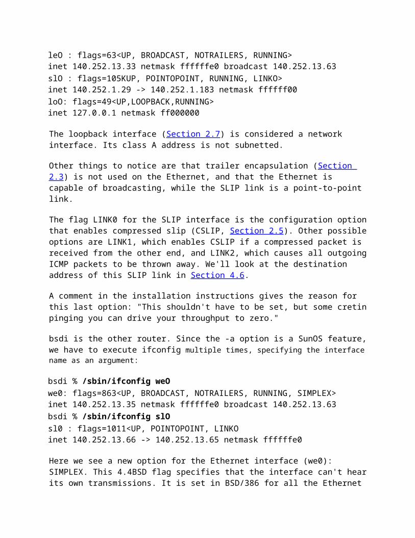
message, a subcode of the ICMP destination unreachable message, to see the additional information returned in an ICMP error message. We'll watch this using UDP (Chapter 11).

One rule of UDP is that if it receives a UDP datagram and the destination port does not correspond to a port that some process has in use, UDP responds with an ICMP port unreachable. We can force a port unreachable using the TFTP client. (We describe TFTP in Chapter 15.)

The well-known UDP port for the TFTP server to be reading from is 69. But most TFTP client programs allow us to specify a different port using the connect command. We use this to specify a port of 8888:

bsdi % tftptftp> connect svr4 8888tftp> get temp.fooTransfer timed out.tftp> quit

specify the hostname and port numbertry to fetch a fileabout 15 seconds later

The connect command saves the name of the host to contact and the port number on that host, for when we later issue the get command. After typing the get command a UDP datagram is sent to port 8888 on host svr4. Figure 6.8 shows the tcpdump output for the exchange of packets that takes place.

Before the UDP datagram can be sent to svr4 an ARP request is sent to determine its hardware address (line 1). The ARP reply (line 2) is returned and then the UDP datagram is sent (line 3). (We have left the ARP request-reply in this tcpdump output to remind us that this exchange may be required before the first IP datagram is sent from one host to the other. In future output we'll delete this exchange if it's not relevant to the topic being discussed.)

12

0.00.002050 (0.0020)

arp who-has svr4 tell bsdiarp reply svr4 is-at 0:0:c0:c2:9b:26

34

0.002723 (0.0007) 0.006399 (0.0037)

bsdi.2924 > svr4.8888: udp 20svr4 > bsdi: icmp: svr4 udp port 8888

56

5.000776 (4.9944)5.004304 (0.0035)

bsdi. 2924 > svr4.8888: udp 20svr4 > bsdi: icmp: svr4 udp port 8888

78

10.000887 (4.9966)10.004416 (0.0035)

bsdi. 2924 > svr4.8888: udp 20svr4 > bsdi: icmp: svr4 udp port 8888

910

15.001014 (4.9966)15.004574 (0.0036)

bsdi.2924 > svr4.8888: udp 20svr4 > bsdi: icmp: svr4 udp port 8888

1112

20.001177 (4.9966)20.004759 (0.0036)

bsdi.2924 > svr4.8888: udp 20 svr4 > bsdi: icmp: svr4 udp port 8888

Figure 6.8 ICMP port unreachable generated by TFTP request.

An ICMP port unreachable is immediately returned (line 4). But the TFTP client appears to ignore the ICMP message, sending another UDP datagram about 5 seconds later (line 5). This continues three more times before the client gives up.

Notice that the ICMP messages are exchanged between hosts, without a port number designation, while each 20-byte UDP datagram is from a specific port (2924) and to a specific port (8888).

The number 20 at the end of each UDP line is the length of the data in the UDP datagram. In this example 20 is the sum of the TFTP's 2-byte opcode, the 9-byte null terminated name temp.foo, and the 9-byte null terminated string netascii. (See Figure 15.1 for the details of the TFTP packet layout.)

If we run this same example using the -e option of tcpdump we see the exact length of each ICMP port unreachable message that's returned to the sender. This length is 70 bytes, and is allocated as shown in Figure 6.9.

Figure 6.9 ICMP message returned for our "UDP port unreachable" example.

One rule of ICMP is that the ICMP error messages (see the final column of Figure 6.3) must include the IP header (including any options) of the datagram that generated the error along with at least the first 8 bytes that followed this IP header. In our example, the first 8 bytes following the IP header contain the UDP header (Figure 11.2).

The important fact is that contained in the UDP header are the source and destination port numbers. It is this destination port number (8888) that caused the ICMP port unreachable to be generated. The source port number (2924) can be used by the system receiving the ICMP error to associate the error with a particular user process (the TFTP client in this example).

One reason the IP header of the datagram that caused the error is sent back is because in this IP header is the protocol field that lets ICMP know how to interpret the 8 bytes that follow (the UDP header in this example). When we look at the TCP header (Figure 17.2) we'll see that the source and destination port numbers are contained in the first 8 bytes of the TCP header. The general format of the ICMP unreachable messages is shown in Figure 6.10.

Figure 6.10 ICMP unreachable message.

In Figure 6.3 we noted that there are 16 different ICMP unreachable messages, codes 0 through 15. The ICMP port unreachable is code 3. Also, although Figure 6.10 indicates that the second 32-bit word in the ICMP message must be 0, the Path MTU Discovery mechanism (Section 2.9) allows a router to place the MTU of the outgoing interface in the low-order 16 bits of this 32-bit value, when code equals 4 ("fragmentation needed but the don't fragment bit is set"). We show an example of this error in Section 11.6.

Although the rules of ICMP allow a system to return more than the first 8 bytes of the data portion of the IP datagram that caused the ICMP error, most Berkeley-derived implementations return exactly 8 bytes. The Solaris 2.2 ip_icmp_return_data_bytes option returns the first 64 bytes of data by default (Section E.4).

tcpdump Time Line

Throughout the text we'll also display the tcpdump output in a time line diagram as shown in Figure 6.11.

Figure 6.11 Time line of TFTP request to an invalid port.

Time increases down the page and the labels on the far left of the figure are the same time values as in our tcpdump output (Figure 6.8). The labels at the top are the hostnames and port numbers for each side of the time line. Be aware that the y-axis down the page is not exactly proportional to the time value. When there is a significant time lag, as between each 5-second retransmission in this example, we'll designate that with a squiggle on both sides of the time line. When UDP or TCP data is being transmitted, we show that packet with a thicker line.

Why does the TFTP client keep retransmitting its request when the ICMP messages are being returned? An element of network programming is occurring in which BSD systems don't notify user processes using UDP of ICMP messages that are received for that socket unless the process has issued a connect on that socket. The standard BSD TFTP client does not issue the connect, so it never receives the ICMP error notification.

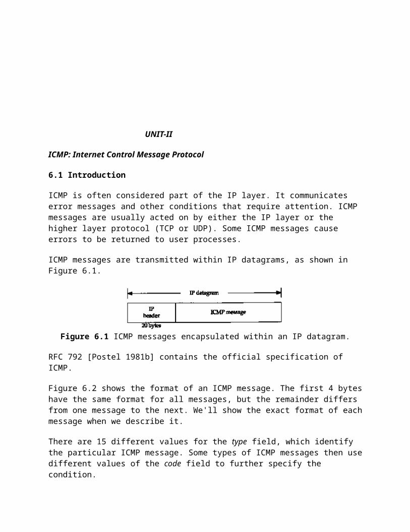
Another point to notice here is the poor retransmission timeout algorithm used by this TFTP client. It just assumes that 5 seconds is adequate and retransmits every 5 seconds, for a total of 25 seconds. We'll see later that TCP has a much better algorithm.

This old-fashioned timeout and retransmission algorithm used by the TFTP client is forbidden by the Host Requirements RFC. Nevertheless, all three systems on the author's subnet, and Solaris 2.2 still use it. AIX 3.2.2 applies an exponential backoff to its timeout, sending packets at 0, 5, 15, and 35 seconds, which is the recommended way We talk much more about timeouts in Chapter 21.

Finally note that the ICMP messages are returned about 3.5 ms after the UDP datagram is sent, which we'll see in Chapter 7 is similar to the round-trip times for Ping replies.

6.6 4.4BSD Processing of ICMP Messages

Since ICMP covers such a wide range of conditions, from fatal errors to informational messages, each ICMP message is handled differently, even within a given implementation. Figure 6.12 is a redo of Figure 6.3, showing the handling performed by 4.4BSD for each of the possible ICMP messages.

If the final column specifies the kernel, that ICMP message is handled by the kernel. If the final column specifies "user process", then that message is passed to all user processes that have registered with the kernel to read received ICMP messages. If there are none of these user processes, the message is silently discarded. (These user processes also receive a copy of all the other ICMP messages, even those handled by the kernel, but only after the kernel has processed the message.) Some messages are completely ignored. Finally, if the final column is a string in quotes, that is the Unix error message corresponding to that condition. Some of these errors, such as TCP's handling of a source quench, we'll cover in later chapters.

type code Description Handled by

0 0 echo reply user process

3 0123456789

101112

destination unreachable:network unreachablehost unreachableprotocol unreachableport unreachablefragmentation needed but DF bit setsource route faileddestination network unknowndestination host unknownsource host isolated (obsolete)dest. network administratively prohibiteddest. host administratively prohibitednetwork unreachable for TOS

"No route to host""No route to host""Connection refused""Connection refused""Message too long""No route to host""No route to host""No route to host""No route to host""No route to host""No route to host""No route to host""No route to host"

131415

host unreachable for TOScommunication administratively prohibitedhost precedence violationprecedence cutoff in effect

(ignored)(ignored)(ignored)

4 0 source quenchkernel for TCP, ignored by UDP

50123

redirect:redirect for networkredirect for hostredirect for type-of-service and networkredirect for type-of-service and host

kernel updates routing tablekernel updates routing tablekernel updates routing tablekernel updates routing table

8 0 echo request kernel generates reply

910

00

router advertisementrouter solicitation

user processuser process

11 01

time exceeded:TTL equals 0 during transitTTL equals 0 during reassembly

user processuser process

12 01

parameter problem:IP header bad (catchall error)required option missing

"Protocol not available""Protocol not available"

1314

00

timestamp requesttimestamp reply

kernel generates replyuser process

1516

00

information request (obsolete)information reply (obsolete)

(ignored)user process

1718

00

address mask requestaddress mask reply

kernel generates replyuser process

Figure 6.12 Handling of the ICMP message types by 4.4BSD.

Ping Program

7.1 Introduction

The name "ping" is taken from the sonar operation to locate objects. The Ping program was written by Mike Muuss and it tests whether another host is reachable. The program sends an ICMP echo request message to a host, expecting an ICMP echo reply to be returned. (Figure 6.3 lists all the ICMP message types.)

Normally if you can't Ping a host, you won't be able to Telnet or FTP to that host. Conversely, if you can't Telnet to a host. Ping is often the starting point to determine what the problem is. Ping also measures the round-trip time to the host, giving us some indication of how "far away" that host is.

In this chapter we'll use Ping as a diagnostic tool and to further explore ICMP. Ping also gives us an opportunity to examine the IP record route and timestamp options. Chapter II of [Stevens 1990] provides the source code for the Ping program.

Years ago we could make the unqualified statement that if we can't Ping a host, we can't Telnet or FTP to that host. With the increased awareness of security on the Internet, routers that provide access control lists, and firewall gateways, unqualified statements like this are no longer true. Reachability ol a given host may depend not only on reachability at the IP layer, but also on what protocol is being used, and the port numbers involved. Ping may show a host as being unreachable, yet we might be able to Telnet to port 25 (the mail server).

7.2 Ping Program

We call the ping program that sends the echo requests the client, and the host being pinged the server. Most TCP/IP implementations support the Ping server directly in the kernel-the server is not a user process. (The two ICMP query services that we described in Chapter 6, the address mask and timestamp requests, are also handled directly by the kernel.)

Figure 7.1 Format of ICMP message for echo request and echo reply.

As with other ICMP query messages, the server must echo the identifier and sequence number fields. Also, any optional data sent by the client must be echoed. These are presumably of interest to the client.

Unix implementations of ping set the identifier field in the ICMP message to the process ID of the sending process. This allows ping to identify the returned responses if there are multiple instances of ping running at the same time on the same host.

The sequence number starts at 0 and is incremented every time a new echo request is sent. ping prints the sequence number of each returned packet, allowing us to see if packets are

missing, reordered, or duplicated. IP is a best effort datagram delivery service, so any of these three conditions can occur.

Historically the ping program has operated in a mode where it sends an echo request once a second, printing each echo reply that is returned. Newer implementations, however, require the -s option to operate this way. By default, these newer implementations send only a single echo request and output "host is alive" if an echo reply is received, or "no answer" if no reply is received within 20 seconds.

LAN Output

ping output on a LAN normally looks like the following:

bsdi % ping svr4PING svr4 (140.252.13.34): 56 data bytes64 bytes from 140.252.13.34: icmp_seq=0 ttl=255 time=0 ms64 bytes from 140.252.13.34: icmp_seq=l ttl=255 time=0 ms64 bytes from 140.252.13.34: icmp_seq=2 ttl=255 time=0 ms64 bytes from 140.252.13.34: icmp_seq=3 ttl=255 time=0 ms64 bytes from 140.252.13.34: icmp_seq=4 ttl=255 time=0 ms64 bytes from 140.252.13.34: icmp_seq=5 ttl=255 time=0 ms64 bytes from 140.252.13.34: icmp_seq=6 ttl=255 time=0 ms64 bytes from 140.252.13.34: icmp_seq=7 ttl=255 time=0 ms^? type interrupt key to stop --- svr4 ping statistics ---8 packets transmitted, 8 packets received, 0% packet lossround-trip min/avg/max = 0/0/0 ms

When the ICMP echo reply is returned, the sequence number is printed, followed by the TTL, and the round-trip time is calculated. (TTL is the time-to-live field in the IP header. The current BSD ping program prints the received TTL each time an echo reply is received-some implementations don't do this. We examine the usage of the TTL in Chapter 8 with the traceroute program.)

As we can see from the output above, the echo replies were returned in the order sent (0, 1,2, and so on).

ping is able to calculate the round-trip time by storing the time at which it sends the echo request in the data portion of the ICMP message. When the reply is returned it subtracts this value from the current time. Notice that on the sending system, bsdi, the round-trip times are all calculated as 0 ms. This is because of the low-resolution timer available to the program. The BSD/386 Version 0.9.4 system only provides a IO-ms timer. (We talk more about this in Appendix B.) We'll see later that when looking at the tcpdump output from this ping example on a system with a finer resolution clock (the Sun) the time difference between the ICMP echo request and its echo reply is just under 4 ms.

The first line of output contains the IP address of the destination host, even though we specified its name (svr4). This implies that the name has been converted to the IP address by a resolver. We examine resolvers and the DNS in Chapter 14. For now realize that if we type a ping command, and a few seconds pass before the first line of output with the IP address is printed, this is the time required for the DNS to determine the IP address corresponding to the hostname. Figure 7.2 shows the tcpdump output for this example.

1 2

0.00.003733 (0.0037)

bsdi > svr4: icmp: echo request svr4 > bsdi: icmp: echo reply

34

0.998045 (0.9943)1.001747 (0.0037)

bsdi > svr4: icmp: echo request svr4 > bsdi: icmp: echo reply

56

1.997818 (0.9961)2.001542 (0.0037)

bsdi > svr4: icmp: echo request svr4 > bsdi: icmp: echo reply

78

2.997610 (0.9961)3.001311 (0.0037)

bsdi > svr4: icmp: echo request svr4 > bsdi: icmp: echo reply

910

3.997390 (0.9961)4.001115 (0.0037)

bsdi > svr4: icmp: echo request svr4 > bsdi: icmp: echo reply

1112

4.997201 (0.9961)5.000904 (0.0037)

bsdi > svr4: icmp: echo request svr4 > bsdi: icmp: echo reply

1314

5.996977 (0.9961)6.000708 (0.0037)

bsdi > svr4: icmp: echo request svr4 > bsdi: icmp: echo reply

1516

6.996764 (0.9961)7.000479 (0.0037)

bsdi > svr4: icmp: echo request svr4 > bsdi: icmp: echo reply

Figure 7.2 ping output across a LAN.

The time between sending the echo request and receiving the echo reply is always 3.7 ms. We can also see that echo requests are sent approximately 1 second apart.

Often the first round-trip time is larger than the rest. This occurs if the destination's hardware address isn't in the ARP cache of the sender. As we saw in Chapter 4, sending an ARP request and getting the ARP reply can take a few milliseconds before the first echo request can be sent. The following example shows this:

sun % arp -a make sun ARP cache is empty

sun % ping svr4PING svr4: 56 data bytes64 bytes from svr4 (140.252.13,34): icmp_seq=0. time=7. ms64 bytes from svr4 (140.252.13.34): icmp_seq=1. time=4. ms64 bytes from svr4 (140.252.13.34): icmp_seq=2. time=4. ms64 bytes from svr4 (140.252.13.34): icmp_seq=3. time=4. ms^? type interrupt key to stop---svr4 PING Statistics---4 packets transmitted, 4 packets received, 0% packet lossround-trip (ms) min/avg/max = 4/4/7

The additional 3 ms in the first RTT is probably for the ARP request and reply

This example was run on the host sun, which provides a timer with microsecond resolution, but the ping program prints the round-trip times with only millisecond resolution. The earlier example, run under BSD/386 Version 0.9.4, printed the round-trip times as 0 ms, since the available timer provided only IO-ms accuracy. The following output is from BSD/386 Version 1.0, which provides a timer with microsecond resolution and a version of ping that prints the higher resolution.

bsdi % ping svr4PING svr4 (140.252.13.34): 56 data bytes64 bytes from 140.252.13.34: icmp_seq=0 ttl=255 time=9.304 ms64 bytes from 140.252.13.34: icmp_seq=1 ttl=255 time=6.089 ms 64 bytes from 140.252.13.34: icmp_seq=2 ttl=255 time=6.079 ms 64 bytes from 140.252.13.34: icmp_seq=3 ttl=255 time=6.096 ms ^? type interrupt key to stop --- svr4 ping statistics ---4 packets transmitted, 4 packets received, 0% packet lossround-trip min/avg/max = 6.079/6.880/9.304 ms

WAN Output

On a wide area network the results can be quite different. The following example was captured on a weekday afternoon, a time when the Internet is normally busy:

gemini % ping vangogh.cs.berkeley.edu PING vangogh.cs.berkeley.edu: 56 data bytes64 bytes from (128.32.130.2): icmp_seq=0. time=660. ms64 bytes from (128.32.130.2): icmp_seq=5. time=1780. ms64 bytes from (128.32.130.2): icmp_seq=7. time=380. ms64 bytes from (128.32.130.2): icmp_seq=8. time=420. ms64 bytes from (128.32.130.2): icmp_seq=9. time=390. ms64 bytes from (128.32.130.2): icmp_seq=14. time=110. ms64 bytes from (128.32.130.2): icmp_seq=15. time=170. ms64 bytes from (128.32.130.2): icmp_seq=16. time=100. ms^? type interrupt key to stop ----vangogh.CS.Berkeley.EDU PING Statistics----17 packets transmitted, 8 packets received, 52% packet lossround-trip (ms) min/avg/max = 100/501/1780

Either the echo requests or the echo replies for sequence numbers 1, 2, 3, 4, 6, 10, II, 12, and 13 were lost somewhere. Note also the large variance in the round-trip times. (This high packet loss rate of 52% is an anomaly. This is not normal for the Internet, even on a weekday afternoon.)

It is also possible across WANs to see packets duplicated (the same sequence number printed two or more times), and to see packets reordered (sequence number N +1 printed before sequence number N).

Hardwired SLIP Links

Let's look at the round-trip times encountered over SLIP links, since they often run at slow asynchronous speeds, such as 9600 bits/sec or less. Recall our serial line throughput calculations in Section 2.10. For this example we'll set the speed of the hardwired SLIP link between hosts bsdi and slip to 1200 bits/sec.

We can estimate the round-trip time as follows. First, notice from the example Ping output shown earlier that by default it sends 56 bytes of data in the ICMP message. With a 20-byte IP header and an 8-byte ICMP header this gives a total IP datagram size of 84 bytes. (We can verify this by running tcpdump -e and seeing the Ethernet frame sizes.) Also, from Section 2.4 we know that at least two additional bytes are added: the END byte at the beginning and end of the datagram. It's also possible for additional bytes to be added by the SLIP framing, but that depends on the value of each byte in the datagram. At 1200 bits/sec with 8 bits per byte, I start bit, and I stop bit, the rate is 120 bytes per second, or 8.33 ms per byte. Our estimate is then (86 x 8.33 x 2), or 1433 ms. (The multiplier of 2 is because we are calculating the round-trip time.)

The following output verifies our calculation:

svr4 % ping -a slipPING slip: 56 data bytes64 bytes from slip (140.252.13.65): icmp_seq=0. time=1480. Ms64 bytes from slip (140.252.13.65): icmp_seq=1. time=1480. Ms 64 bytes from slip (140.252.13.65): icmp_seq=2. time=1480. Ms 64 bytes from slip (140.252.13.65): icmp_seq=3. time=1480. Ms ^?----slip PING Statistics----5 packets transmitted, 4 packets received, 20% packet lossround-trip (ms) min/avg/max = 1480/1480/1480

(The -s option is required for SVR4 to send one request every second.) The round-trip time is almost 1.5 seconds but the program is still sending out each ICMP echo request at 1-second intervals. This means there are two outstanding echo requests (sent at time 0 and time 1) before the first reply comes back (at time 1.480). That's also why the summary line says one packet has been lost. It really hasn't been lost, it's probably still on its way back.

We'll return to this slow SLIP link in Chapter 8 when we examine the traceroute program.

Dialup SLIP Links

The conditions change with a dialup SLIP link since we now have modems on each end of the link. The modems being used between the systems sun and netb provide what is called V.32 modulation (9600 bits/sec), V.42 error control (also called LAP-M), and V.42bis data compression. This means that our simple calculations, which were fairly accurate for a hardwired link where we knew all the parameters, become less accurate.

Numerous factors are at work. The modems introduce some latency. The size of the packets may decrease with the data compression, but the size may then increase to a multiple of the packet size used by the error control protocol. Also the receiving modem can't release received data bytes until the cyclic redundancy character (the checksum) has been verified. Finally, we're dealing with a computer's asynchronous serial interface on each end, and many operating systems read these interfaces only at fixed intervals, or when a certain number of characters have been received.

As an example, we ping the host gemini from the host sun:

sun % ping geminiPING gemini: 56 data bytes64 bytes from gemini (140.252.1.11): icmp_seq=0. time=373. ms64 bytes from gemini (140.252.1.11): icmp_seq=l. time=360. ms 64 bytes from gemini (140.252.1.11): icmp_seq=2. time=340. ms 64 bytes from gemini (140.252.1.11): icmp_seq=3. time-320. ms 64 bytes from gemini (140.252.1.11): icmp_seq=4. time=330. ms 64 bytes from gemini (140.252.1.11): icmp seq=5. time=310. ms 64 bytes from gemini (140.252.1.11): icmp seq=6. time==290. ms 64 bytes from gemini (140.252.1.11): icmp_seq-7. time=300. ms 64 bytes from gemini (140.252.1.11): icmp_seq=8. time=280. ms 64 bytes from gemini (140.252.1.11): icmp_seq=9. time=290. ms 64 bytes from gemini (140.252.1.11): icmp_seq=10. time=300. ms 64 bytes from gemini (140.252.1.11): icmp_seq=ll. time=280. ms --gemini PING Statistics--12 packets transmitted, 12 packets received, 0% packet lossround-trip (ms) min/avg/max = 280/314/373

Note that the first RTT is not a multiple of 10 ms, but every other line is. If we run this numerous times, we see this property every time. (This is not caused by the resolution of the clock on the host sun, because we know that its clock provides millisecond resolution from the tests we run in Appendix B.)

Also note that the first RTT is larger than the next, and they keep decreasing, and then they range between 280 and 300 ms. If we let it run for a minute or two, the RTTs stay in this range, never going below 260 ms. If we calculate the expected RTT at 9600 bits/sec (Exercise 7.2) we get 180 ms, so our observed values are about 1.5 times the expected value.

If we run ping for 60 seconds and look at the average RTT it calculates, we find that with V.42 and V.42bis our average is 277 ms. (This is better than the average printed for our preceding example, because we ran it longer to amortize the longer RTTs at the beginning.) If we turn off just the V.42bis data compression our average is 330 ms. If we turn off the V.42 error control (which also turns off the V.42bis data compression) our average is 300 ms. These modem parameters do affect the RTTs, and using the error control and data compression appears to be the best.

7.3 IP Record Route Option

The ping program gives us an opportunity to look at the IP record route (RR) option. Most versions of ping provide the -R option that enables the record route feature. It causes ping to set the IP RR option in the outgoing IP datagram (which contains the ICMP echo request message). This causes every router that handles the datagram to add its IP address to a list in the options field. When the datagram reaches the final destination, the list of IP addresses should be copied into the outgoing ICMP echo reply, and all the routers on the return path also add their IP addresses to the list. When ping receives the echo reply it prints the list of IP addresses.

As simple as this sounds, there are pitfalls. Generation of the RR option by the source host, processing of the RR option by the intermediate routers, and reflection of the incoming RR list in an ICMP echo request into the outgoing ICMP echo reply are all optional features. Fortunately, most systems today do support these optional features, but some systems don't reflect the IP list.

The biggest problem, however, is the limited room in the IP header for the list of IP addresses. We saw in Figure 3.1 that the header length in the IP header is a 4-bit field, limiting the entire IP header to 15 32-bit words (60 bytes). Since the fixed size of the IP header is 20 bytes, and the RR option uses 3 bytes for overhead (which we describe below), this leaves 37 bytes (60-20-3) for the list, allowing up to nine IP addresses. In the early days of the ARPANET, nine IP addresses seemed like a lot, but since this is a round-trip list (in the case of the -R option for ping), it's of limited use today. (In Chapter 8 we'll look at the Traceroute tool for determining the route followed by a datagram.) Despite these shortcomings, the record route option works and provides an opportunity to look in detail at the handling of IP options. Figure 7.3 shows the general format of the RR option in the IP datagram.

Figure 7.3 General format of record route option in IP header.

Code is a I-byte field specifying the type of IP option. For the RR option its value is 7. Len is the total number of bytes of the RR option, which in this case is 39. (Although it's possible to specify an RR option with less than the maximum size, ping always provides a 39-byte option field, to record up to nine IP addresses. Given the limited room in the IP header for options, it doesn't make sense to specify a size less than the maximum.)

Ptr is called the pointer field. It is a 1-based index into the 39-byte option of where to store the next IP address. Its minimum value is 4, which is the pointer to the first IP address. As each IP address is recorded into the list, the value of ptr becomes 8, 12, 16, up to 36. After the ninth address is recorded ptr becomes 40, indicating the list is full.

When a router (which by definition is multihomed) records its IP address in the list, which IP address is recorded? It could be the address of the incoming interface or the outgoing interface. RFC 791 [Postel 1981a] specifies that the router records the outgoing IP address. We'll see that when the originating host (the host running ping) receives the ICMP echo reply with the RR option enabled, it also records its incoming IP address in the list.

Normal Example

Let's run an example of the RR option with the ping program. We'll run ping on the host svr4 to the host slip. One intermediate router (bsdi) will handle the datagram. The following output is from svr4:

svr4 % ping -R slipPING slip (140.252.13.65): 56 data bytes64 bytes from 140.252.13.65: icmp_seq=0 ttl=254 time=280 msRR: bsdi (140.252.13.66)slip (140.252.13.65)bsdi (140.252.13.35)svr4 (140.252.13.34)64 bytes from 140.252.13.65: icmp_seq=1 ttl=254 time=280 ms (same route)64 bytes from 140.252.13.65: icmp_seq=2 ttl=254 time=270 ms (same route)^?--- slip ping statistics ---3 packets transmitted, 3 packets received, 0% packet lossround-trip min/avg/max = 270/276/280 ms

Figure 7.4 shows the four hops that the packets take (two in each direction), and which hop adds which IP address to the RR list.

Figure 7.4 ping with record route option.

The router bsdi adds a different IP address to the list in each direction. It always adds the IP address of the outgoing interface. We can also see that when the ICMP echo reply reaches the originating system (svr4) it adds the IP address of the incoming interface to the list.

We can also watch this exchange of packets from the host sun, running tcpdump with its -v option (to see the IP options). Figure 7.5 shows the output.

1 0.0 svr4 > slip: icmp: echo request (ttl 32, id 35835,optlen=40 RR{39}=RR(#0.0.0.0/0.0.0.0/0.0.0.0/0.0.0.0/0.0.0.0/0.0.0.0/0.0.0.0/0.0.0.0/0.0.0.0} EOL)

20.267746 (0.2677)

slip > svr4: icmp: echo reply (ttl 254, id 1976,optlen=40 RR{39}= RR(140.252.13.66/140.252.13.65/140.252.13.35/#0.0.0.0/0.0.0.0/0.0.0.0/0.0.0.0/0.0.0.0/0.0.0.0} EOL)

Figure 7.5 tcpdump output of record route option.

The output optlen=40 indicates there are 40 bytes of option space in the IP header. (Recall that the length of the IP header must be a multiple of 4 bytes.) RR{39} means the record route option is present, and its length field is 39. The list of nine IP addresses is then shown, with a pound sign (#) indicating which IP address is pointed to by the ptr field in the RR option header. Since we are watching these packets on the host sun (see Figure 7.4) we only see the ICMP echo request with the empty list, and the ICMP echo reply with three addresses in the list. We have deleted the remaining lines in the tcpdump output, since they are nearly identical to what we show in Figure 7.5.

The notation EOL at the end of the record route information indicates the IP option "end of list" value appeared. The EOL option has a value of 0. What's happening is that 39 bytes of RR data are in the 40 bytes of option space in the IP header. Since the option space is set to 0 before the datagram is sent, this final byte of 0 that follows the 39 bytes of RR data is interpreted as an EOL. That is what we want to have happen. If there are multiple options in the option field of the IP header, and pad bytes are needed before the next option starts, the other special character NOP ("no operation"), with a value of 1, can be used.

In Figure 7.5, SVR4 sets the TTL field of the echo request to 32, and BSD/386 sets it to 255. (It prints as 254 since the router bsdi has already decremented it by one.) Newer systems are setting the TTL of ICMP messages to the maximum (255).

It turns out that of the three TCP/IP implementations used by the author, both BSD/386 and SVR4 support the record route option. That is, they correctly update the RR list when forwarding a datagram, and they correctly reflect the RR list from an incoming ICMP echo request to the outgoing ICMP echo reply. SunOS 4.1.3, however, updates the RR list when forwarding a datagram, but does not reflect the RR list. Solaris 2.x corrects this problem.

Abnormal Output

The following example was seen by the author and provides a starting point for our description of the ICMP redirect message in Chapter 9. We ping the host aix on the 140.252.1 subnet (accessible through the dialup SLIP connection on the host sun) with the record route option. We get the following output, when run on the host slip:

slip % ping -R aixPING aix (140.252.1.92): 56 data bytes64 bytes from 140.252.1.92: icmp_seq-0 ttl=-251 time-650 msRR: bsdi (140.252.13.35)sun (140.252.1.29)netb (140.252.1.183)aix (140.252.1.92)gateway (140.252.1.4) why is this router used?netb (140.252.1.183)sun (140.252.13.33)bsdi (140.252.13.66)slip (140.252.13.65)64 bytes from aix: icmp_seq=l ttl=251 time=610 ms (same route) 64 bytes from aix: icmp_seq=2 ttl=251 time"600 ms (same route) ^?-- aix ping statistics -4 packets transmitted, 3 packets received, 25% packet lossround-trip min/avg/max = 600/620/650 ms

We could have run this example from the host bsdi. We chose to run it from slip to see all nine IP addresses in the RR list used.

The puzzle in this output is why the outgoing datagram (the ICMP echo request) went directly from netb to aix, but the return (the ICMP echo reply) went from aix, through the router gateway, before going to netb. What we're seeing here is a feature of IP routing that we describe below. Figure 7.6 shows the path of the datagrams.

Figure 7.6 ping with record route, showing IP routing feature.

The problem is that aix does not know to send IP datagrams destined for the subnet 140.252.13 to netb. Instead, aix has a default entry in its routing table that tells it to send all datagrams to the router gateway if it doesn't have a particular route for the destination. The router gateway has more routing knowledge than any of the hosts on the 140.252.1 subnet. (There are more than 150 hosts on this Ethernet and instead of running a routing daemon on every one, each has a "default" entry that points to the router gateway.)

An unanswered question here is why doesn't gateway send an ICMP redirect (Section 9.5) to aix to update its routing table? For some reason (perhaps that the datagram generating the redirect is an ICMP echo request message) the redirect is not generated. But if we use Telnet and connect to the daytime server on aix, the ICMP redirect is generated, and the routing table on aix is updated. If we then execute ping with the record route option enabled, the route shows that the datagrams go from netb to aix and back to netb, without the extra hop to the router gateway. We'll look at these ICMP redirects in more detail in Section 9.5.

7.4 IP Timestamp Option

The IP timestamp option is similar to the record route option. Figure 7.7 shows the format of the IP timestamp option (compare with Figure 7.3).

Figure 7.7 General format of timestamp option in IP header.

The code field is 0x44 for the timestamp option. The two fields len and ptr are the same as for the record route option: the total length of the option (normally 36 or 40) and a pointer to the next available entry (5,9, 13, etc.).

The next two fields are 4-bit values: OF is the overflow field and FL is a flags field. The operation of the timestamp option is driven by the flags field, as shown in Figure 7.8.

flags Description

0 Record only timestamps. This is what we show in Figure 7.7.

1Each router records its IP address and its timestamp. There is room for only four of these pairs in the options list.

3The sender initializes the options list with up to four pairs of IP addresses and a 0 timestamp. A router records its timestamp only if the next IP address in the list matches the router's.

Figure 7.8 Meaning of the flags value for timestamp option.

If a router can't add a timestamp because there's no room left, it just increments the overflow field.

The preferred value for the timestamps is the number of milliseconds past midnight, UTC, similar to the ICMP timestamp request and reply (Section 6.4). If this format is not available to a router, it can insert whatever time representation that it uses, but must then turn on the high-order bit of the timestamp to indicate the nonstandard value.

Given the limitations that we encountered with the record route option, things get worse with the timestamp option. If we record both IP addresses and timestamps (a flags of 1), we can store only four of these pairs. Recording only timestamps is next to useless because we have no indication regarding which timestamp corresponds to which router (unless we have a fixed topology that never changes). A flags of 3 is better, as we can then select which routers insert their timestamp. A more fundamental problem is that you probably have no control over how accurate the timestamp is at any given router. This makes it fruitless to try to measure hop times between routers using this IP option. We'll see that the traceroute program (Chapter 8) provides a better way of measuring hop times between routers.

7.5 Summary

The ping program is the basic connectivity test between two systems running TCP/IP. It uses the ICMP echo request and echo reply messages and does not use a transport layer (TCP or UDP). The Ping server is normally part of the kernel's ICMP implementation.

We looked at the normal ping output for a LAN, WAN, and SLIP links (dialup and hardwired), and performed some serial line throughput calculations for a dedicated SLIP link. ping also let us examine and use the IP record route option. We used this IP option to

see how default routes are often used, and will return to this topic in Chapter 9. We also looked at the IP timestamp option, but it is of limited practical use.

Exercises

7.1 Draw a time line for the ping output for the SLIP link in Section 7.2.

7.2 Calculate the RTT if the SLIP link between bsdi and slip is set to 9600 bits/sec. Assume the default of 56 bytes of data.

7.3 The current BSD ping program allows us to specify a pattern for the data portion of the ICMP message. (The first 8 bytes of the data portion are not filled with the pattern, since the time at which the packet is sent is stored here.) If we specify a pattern of 0xc0, recalculate the answer to the previous exercise. (Hint: Reread Section 2.4.)

7.4 Does the use of compressed SLIP (CSLIP, Section 2.5) affect the ping times that we observed in Section 7.2?

7.5 Examine Figure 2.4. Do you expect any difference between a ping of the loopback address, versus a ping of the host's Ethernet address?

Traceroute Program

8.1 Introduction

The Traceroute program, written by Van Jacobson, is a handy debugging tool that allows us to further explore the TCP/IP protocols. Although there are no guarantees that two consecutive IP datagrams from the same source to the same destination follow the same route, most of the time they do. Traceroute lets us see the route that IP datagrams follow from one host to another. Traceroute also lets us use the IP source route option.

The manual page states: "Implemented by Van Jacobson from a suggestion by Steve Deering. Debugged by a cast of thousands with particularly cogent suggestions or fixes from C. Philip Wood, Tim Seaver, and Ken Adelman."

8.2 Traceroute Program Operation

In Section 7.3 we described the IP record route option (RR). Why wasn't this used instead of developing a new application? There are three reasons. First, historically not all routers have supported the record route option, making it unusable on certain paths. (Traceroute doesn't require any special or optional features at any intermediate routers.)

Second, record route is normally a one-way option. The sender enables the option and the receiver has to fetch all the values from the received IP header and somehow return them to the sender. In Section 7.3 we saw that most implementations of the Ping server (the ICMP echo reply function within the kernel) reflect an incoming RR list, but this doubles the

number of IP addresses recorded (the outgoing path and the return path), which runs into the limit described in the next paragraph. (Traceroute requires only a working UDP module at the destination-no special server application is required.)

The third and major reason is that the room allocated for options in the IP header isn't large enough today to handle most routes. There is room for only nine IP addresses in the IP header options field. In the old days of the ARPANET this was adequate, but it is far too small nowadays.

Traceroute uses ICMP and the TTL field in the IP header. The TTL field (time-to-live) is an 8-bit field that the sender initializes to some value. The recommended initial value is specified in the Assigned Numbers RFC and is currently 64. Older systems would often initialize it to 15 or 32. We saw in some of the Ping examples in Chapter 7 that ICMP echo replies are often sent with the TTL set to its maximum value of 255.

Each router that handles the datagram is required to decrement the TTL by either one or the number of seconds that the router holds onto the datagram. Since most routers hold a datagram for less than a second, the TTL field has effectively become a hop counter, decremented by one by each router.

RFC 1009 [Braden and Postel 1987] required a router that held a datagram for more than 1 second to decrement the TTL by the number of seconds. Few routers implemented this requirement. The new Router Requirements RFC [Almquist 1993] makes this optional, allowing a router to treat the TTL as just a hop count.

The purpose of the TTL field is to prevent datagrams from ending up in infinite loops, which can occur during routing transients. For example, when a router crashes or when the connection between two routers is lost, it can take the routing protocols some time (from seconds to a few minutes) to detect the lost route and work around it. During this time period it is possible for the datagram to end up in routing loops. The TTL field puts an upper limit on these looping datagrams.

When a router gets an IP datagram whose TTL is either 0 or 1 it must not forward the datagram. (A destination host that receives a datagram like this can deliver it to the application, since the datagram does not have to be routed. Normally, however, no system should receive a datagram with a TTL of 0.) Instead the router throws away the datagram and sends back to the originating host an ICMP "time exceeded" message. The key to Traceroute is that the IP datagram containing this ICMP message has the router's IP address as the source address.

We can now guess the operation of Traceroute. It sends an IP datagram with a TTL of 1 to the destination host. The first router to handle the datagram decrements the TTL, discards the datagram, and sends back the ICMP time exceeded. This identifies the first router in the path. Traceroute then sends a datagram with a TTL of 2, and we find the IP address of the second router. This continues until the datagram reaches the destination host. But even though the arriving IP datagram has a TTL of 1, the destination host won't throw it away

and generate the ICMP time exceeded, since the datagram has reached its final destination. How can we determine when we've reached the destination?

Traceroute sends UDP datagrams to the destination host, but it chooses the destination UDP port number to be an unlikely value (larger than 30,000), making it improbable that an application at the destination is using that port. This causes the destination host's UDP module to generate an ICMP "port unreachable" error (Section 6.5) when the datagram arrives. All Traceroute needs to do is differentiate between the received ICMP messages-time exceeded versus port unreachable-to know when it's done.

The Traceroute program must be able to set the TTL field in the outgoing datagram. Not all programming interfaces to TCP/IP support this, and not all implementations support the capability, but most current systems do, and are able to run Traceroute. This programming interface normally requires the user to have superuser privilege, meaning it may take special privilege to run it on your host.

UNIT-III

IP Routing

9.1 Introduction

Routing is one of the most important functions of IP. Figure 9.1 shows a simplified view of the processing done at the IP layer. Datagrams to be routed can be generated either on the local host or on some other host. In the latter case this host must be configured to act as a router, or datagrams received through the network interfaces that are not ours are dropped (i.e., silently discarded).

In Figure 9.1 we also show a routing daemon, which is normally a user process. The most common daemons used on Unix systems are the programs routed and gated. (The term daemon means the process is running "in the background," carrying out operations on behalf of the whole system. Daemons are normally started when the system is

bootstrapped and run as long as the system is up.) The topics of which routing protocol to use on a given host, how to exchange routing information with adjacent routers, and how the routing protocols work are complex and can fill an entire book of their own. (Interested readers are referred to [Periman 1992] for many of the details.) We'll look briefly at dynamic routing and the Routing Information Protocol (RIP) in Chapter 10. Our main interest in the current chapter is how a single IP layer makes its routing decisions.

The routing table that we show in Figure 9.1 is accessed frequently by IP (on a busy host this could mean hundreds of times a second) but is updated much less frequently by a routing daemon (possibly about once every 30 seconds). The routing table can also be updated when ICMP "redirect" messages are received, something we'll look at in Section 9.5, and by the route command. This command is often executed when the system is bootstrapped, to install some initial routes. We'll also use the netstat command in this chapter to display the routing table.

Figure 9.1 Processing done at the IP layer.

9.2 Routing Principles

The place to start our discussion of IP routing is to understand what is maintained by the kernel in its routing table. The information contained in the routing table drives all the routing decisions made by IP.

In Section 3.3 we listed the steps that IP performs when it searches its routing table.

1. Search for a matching host address. 2. Search for a matching network address.

3. Search for a default entry. (The default entry is normally specified in the routing table as a network entry, with a network ID of 0.)

A matching host address is always used before a matching network address.

The routing done by IP, when it searches the routing table and decides which interface to send a packet out, is a routing mechanism. This differs from a routing policy, which is a set of rules that decides which routes go into the routing table. IP performs the routing mechanism while a routing daemon normally provides the routing policy.

Simple Routing Table

Let's start by looking at some typical host routing tables. On the host svr4 we execute the netstat command with the -r option to list the routing table and the -n option, which prints IP addresses in numeric format, rather than as names. (We do this because some of the entries in the routing table are for networks, not hosts. Without the -n option, the netstat command searches the file /etc/networks for the network names. This confuses the discussion by adding another set of names-network names in addition to hostnames.)

svr4 % netstat -rn Routing tablesDestination 140.252.13.65127.0.0.1default140.252.13.32

Gateway140.252.13.35127.0.0.1140.252.13.33140.252.13.34

FlagsUGHUHUGU

Refcnt0104

Use00025043

Interfaceemd0lo0emd0emd0

The first line says for destination 140.252.13.65 (host slip) the gateway (router) to send the packet to is 140.252.13.35 (bsdi). This is what we expect, since the host slip is connected to bsdi with a SLIP link, and bsdi is on the same Ethernet as this host. There are five different flags that can be printed for a given route.

U The route is up.G The route is to a gateway (router). If this flag is not set, the destination is directly connected. H The route is to a host, that is, the destination is a complete host address. If this flag is not set, the route is to a network, and the destination is a network address: a net ID, or a combination of a net ID and a subnet ID. D The route was created by a redirect (Section 9.5).M The route was modified by a redirect (Section 9.5).

The G flag is important because it differentiates between an indirect route and a direct route. (The G flag is not set for a direct route.) The difference is that a packet going out a

direct route has both the IP address and the link-layer address specifying the destination (Figure 3.3). When a packet is sent out an indirect route, the IP address specifies the final destination but the link-layer address specifies the gateway (that is, the next-hop router). We saw an example of this in Figure 3.4. In this routing table example we have an indirect route (the G flag is set) so the IP address of a packet using this route is the final destination (140.252.13.65), but the link-layer address must correspond to the router 140.252.13.35.

It's important to understand the difference between the G and H flags. The G flag differentiates between a direct and an indirect route, as described above. The H flag, however, specifies that the destination address (the first column of netstat output) is a complete host address. The absence of the H flag means the destination address is a network address (the host ID portion will be 0). When the routing table is searched for a route to a destination IP address, a host address entry must match the destination address completely, while a network address only needs to match the network ID and any subnet ID of the destination address. Also, some versions of the netstat command print all the host entries first, followed by the network entries.

The reference count column gives the number of active uses for each route. A connection-oriented protocol such as TCP holds on to a route while the connection is established. If we established a Telnet connection between the two hosts svr4 and slip, we would see the reference count go to 1. With another Telnet connection the reference count would go to 2, and so on.

The next column ("use") displays the number of packets sent through that route. If we are the only users of the route and we run the ping program to send 5 packets, the count goes up by 5. The final column, the interface, is the name of the local interface.

The second line of output is for the loopback interface (Section 2.7), always named lo0. The G flag is not set, since the route is not to a gateway. The H flag indicates that the destination address (127.0.0.1) is a host address, and not a network address. When the G field is not set, indicating a direct route, the gateway column gives the IP address of the outgoing interface.

The third line of output is for the default route. Every host can have one or more default routes. This entry says to send packets to the router 140.252.13.33 (sun) if a more specific route can't be found. This means the current host (svr4) can access other systems across the Internet through the router sun (and its SLIP link), using this single routing table entry. Being able to establish a default route is a powerful concept. The flags for this route (UG) indicate that it's a route to a gateway, as we expect.

Here we purposely call sun a router and not a host because when it's used as a default router, its IP forwarding function is being used, not its host functionality.

The Host Requirements RFC specifically states that the IP layer must support multiple default routes. Many implementations, however, don't support this. When multiple default

routes exist, a common technique is to round robin among them. This is what Solaris 2.2 does, for example.

The final line of output is for the attached Ethernet. The H flag is not set, indicating that the destination address (140.252.13.32) is a network address with the host portion set to 0. Indeed, the low-order 5 bits are 0 (Figure 3.11). Since this is a direct route (the G flag is not set) the gateway column specifies the IP address of the outgoing interface.

Implied in this final entry, but not shown by the netstat output, is the mask associated with this destination address (140.252.13.32). If this destination is being compared against the IP address 140.252.13.33, the address is first logically ANDed with the mask associated with the destination (the subnet mask of the interface, 0xffffffe0, from Section 3.7) before the comparison. For a network route to a directly connected network, the routing table mask defaults to the subnet mask of the interface. But in general the routing table mask can assume any 32-bit value. A value other than the default can be specified as an option to the route command.

The complexity of a host's routing table depends on the topology of the networks to which the host has access.

1. The simplest (but least interesting) case is a host that is not connected to any networks at all. The TCP/IP protocols can still be used on the host, but only to communicate with itself! The routing table in this case consists of a single entry for the loopback interface.

2. Next is a host connected to a single LAN, only able to access hosts on that LAN. The routing table consists of two entries: one for the loopback interface and one for the LAN (such as an Ethernet).

3. The next step occurs when other networks (such as the Internet) are reachable through a single router. This is normally handled with a default entry pointing to that router.

4. The final step is when other host-specific or network-specific routes are added. In our example the route to the host slip, through the router bsdi, is an example of this.

Let's follow through the steps IP performs when using this routing table to route some example packets on the host svr4.

1. Assume the destination address is the host sun, 140.252.13.33. A search is first made for a matching host entry. The two host entries in the table (slip and localhost) don't match, so a search is made through the routing table again for a matching network address. A match is found with the entry 140.252.13.32 (the network IDs and subnet IDs match), so the emd0 interface is used. This is a direct route, so the link-layer address will be the destination address.

2. Assume the destination address is the host slip, 140.252.13.65. The first search through the table, for a matching host address, finds a match. This is an indirect

route so the destination IP address remains 140.252.13.65, but the link-layer address must be the link-layer address of the gateway 140.252.13.35, and the interface is emd0.

3. This time we're sending a datagram across the Internet to the host aw.com (192.207.117.2). The first search of the routing table for a matching host address fails, as does the second search for a matching network address. The final step is a search for a default entry, and this succeeds. The route is an indirect route through the gateway 140.252.13.33 using the interface emd0.

4. In our final example we send a datagram to our own host. There are four ways to do this, using either the hostname, the host IP address, the loopback name, or the loopback IP address:

ftp svr4 ftp140.252.13.34

ftp localhostftp 127.0.0.1

In the first two cases, the second search of the routing table yields a network match with 140.252.13.32, and the packet is sent down to the Ethernet driver. As we showed in Figure 2.4 it will be seen that this packet is destined for the host's own IP address, and the packet is sent to the loopback driver, which sends it to the IP input queue.

In the latter two cases, specifying the name of the loopback interface or its IP address, the first search of the routing table finds the matching host address entry, and the packet is sent to the loopback driver, which sends it to the IP input queue.

In all four cases the packet is sent to the loopback driver, but two different routing decisions are made.

Initializing a Routing Table

We never said how these routing table entries are created. Whenever an interface is initialized (normally when the interface's address is set by the ifconfig command) a direct route is automatically created for that interface. For point-to-point links and the loopback interface, the route is to a host (i.e., the H flag is set). For broadcast interfaces such as an Ethernet, the route is to that network.

Routes to hosts or networks that are not directly connected must be entered into the routing table somehow. One common way is to execute the route command explicitly from the initialization files when the system is bootstrapped. On the host svr4 the following two commands were executed to add the entries that we showed earlier:

route add default sun 1route add slip bsdi 1

The third arguments (default and slip) are the destinations, the fourth argument is the gateway (router), and the final argument is a routing metric. All that the route command does with this metric is install the route with the G flag set if the metric is greater than 0, or without the G flag if the metric is 0.

Unfortunately, few systems agree on which start-up file contains the route commands. Under 4.4BSD and BSD/386 it is /etc/netstart, under SVR4 it is /etc/inet/rc.inet, under Solaris 2.x it is /etc/rc2.d/S69inet, SunOS 4.1.x uses /etc/rc.local, and AIX 3.2.2 uses /etc/rc.net.

Some systems allow a default router to be specified in a file such as /etc/defaultrouter, and this default is added to the routing table on every reboot.

Other ways to initialize a routing table are to run a routing daemon (Chapter 10) or to use the newer router discovery protocol (Section 9.6).

A More Complex Routing Table

The host sun is the default router for all the hosts on our subnet, since it has the dialup SLIP link that connects to the Internet (see the figure on the inside front cover).

sun % netstat -rn Routing tablesDestination Gateway Flags Refcnt Use Interface 140.252.13.65 140.252.13.35 UGH 0 171 le0127.0.0.1 127.0.0.1 UH 1 766 lo0140.252.1.183 140.252.1.29 UH 0 0 sl0default 140.252.1.183 UG 1 2955 sl0140.252.13.32 140.252.13.33 U 8 99551 le0

The first two entries are identical to the first two for the host svr4: a host-specific route to slip through the router bsdi, and the loopback route.

The third line is new. It is a direct route (the G flag is not set) to a host (the H flag is set) and corresponds to our point-to-point link, the SLIP interface. If we compare it to the output from the ifconfig command,

sun % ifconfig sl0sl0: flags=1051<UP,POINTOPOINT,RUNNING>inet 140.252.1.29 -> 140.252.1.183 netmask ffffff00

we see that the destination address in the routing table is the other end of the point-to-point link (the router netb) and the gateway address is really the local IP address of the outgoing interface (140.252.1.29). (We said earlier that the gateway address printed by netstat for a direct route is the local IP address of the interface to use.)

The default entry is an indirect route (G flag) to a network (no H flag), as we expect. The gateway address is the address of the router (140.252.1.183, the other end of the SLIP link) and not the local IP address of the SLIP link (140.252.1.29). Again, this is because it is an indirect route, not a direct route.

We should also note that the third and fourth lines output by netstat (the ones with an interface of sl0) are created by the SLIP software being used when the SLIP line is brought up, and deleted when the SLIP link is brought down.

No Route to Destination

All our examples so far have assumed that the search of the routing table finds a match, even if the match is the default route. What if there is no default route, and a match isn't found for a given destination?

The answer depends on whether the IP datagram being routed was generated on the host or is being forwarded (e.g., we're acting as a router). If the datagram was generated on this host, an error is returned to the application that sent the datagram, either "host unreachable" or "network unreachable." If the datagram was being forwarded, an ICMP host unreachable error is sent back to original sender. We examine this error in the following section.

9.3 ICMP Host and Network Unreachable Errors

The ICMP "host unreachable" error message is sent by a router when it receives an IP datagram that it cannot deliver or forward. (Figure 6.10 shows the format of the ICMP unreachable messages.) We can see this easily on our network by taking down the dialup SLIP link on the router sun, and trying to send a packet through the SLIP link from any of the other hosts that specify sun as the default router.

Older implementations of the BSD TCP/IP software generated either a host unreachable, or a network unreachable, depending on whether the destination was on a local subnet or not. 4.4BSD generates only the host unreachable.

Recall from the netstat output for the router sun shown in the previous section that the routing table entries that use the SLIP link are added when the SLIP link is brought up, and deleted when the SLIP link is brought down. This means that when the SLIP link is down, there is no default route on sun. But we don't try to change all the other host's routing tables on our small network, having them also remove their default route. Instead we count on the ICMP host unreachable generated by sun for any packets that it gets that it cannot forward.

We can see this by running ping on svr4, for a host on the other side of the dialup SLIP link (which is down):

svr4 % ping geminiICMP Host Unreachable from gateway sun (140.252.13.33) ICMP Host Unreachable from gateway sun (140.252.13.33)^? type interrupt key to stop

Figure 9.2 shows the tcpdump output for this example, run on the host bsdi.

1 2

0.00.00 (0.00)

svr4 > gemini: icmp: echo requestsun > svr4: icmp: host gemini unreachable

34

0.99 (0.99)0.99 (0.00)

svr4 > gemini: icmp: echo requestsun > svr4: icmp: host gemini unreachable

Figure 9.2 ICMP host unreachable in response to ping.

When the router sun finds no route to the host gemini, it responds to the echo request with a host unreachable.

If we bring the SLIP link to the Internet up, and try to ping an IP address that is not connected to the Internet, we expect an error. What is interesting is to see how far the packet gets into the Internet, before the error is returned:

sun % ping 192.82.148.1 this IP address is not connected to the InternetPING 192.82.148.1: 56 data bytesICMP Host Unreachable from gateway enss142.UT.westnet.net (192.31.39.21) for icmp from sun (140.252.1.29) to 192.82.148.1

Looking at Figure 8.5 we see that the packet made it through six routers before detecting that the IP address was invalid. Only when it got to the border of the NSFNET backbone was the error detected. This implies that the six routers that forwarded the packet were doing so because of default entries, and only when it reached the NSFNET backbone did a router have complete knowledge of every network connected to the Internet. This illustrates that many routers can operate with just partial knowledge of the big picture.

[Ford, Rekhter, and Braun 1993] define a top-level routing domain as one that maintains routing information to most Internet sites and does not use default routes. They note that five of these top-level routing domains exist on the Internet: the NFSNET backbone, the Commercial Internet Exchange (CIX), the NASA Science Internet (NSI), SprintLink, and the European IP Backbone (EBONE).

9.4 To Forward or Not to Forward

We've mentioned a few times that hosts are not supposed to forward IP datagrams unless they have been specifically configured as a router. How is this configuration done?

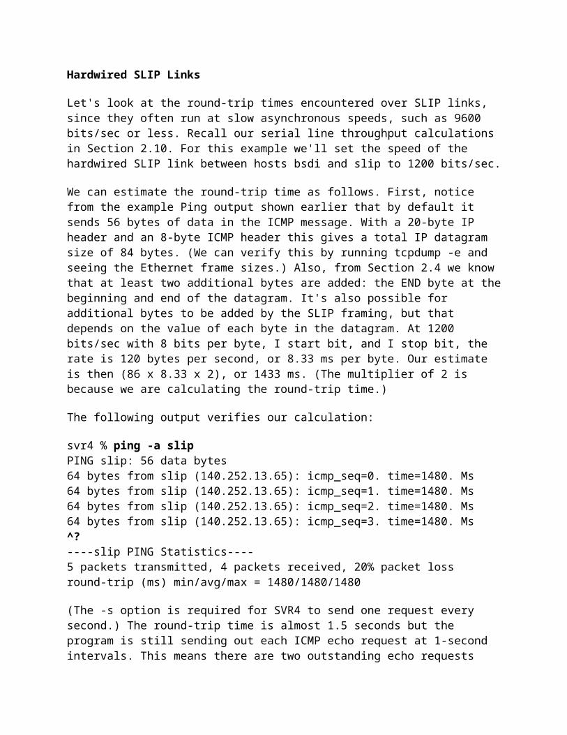
Most Berkeley-derived implementations have a kernel variable named ipforwarding, or some similar name. (See Appendix E.) Some systems (BSD/386 and SVR4, for example) only forward datagrams if this variable is nonzero. SunOS 4.1.x allows three values for the variable: -1 means never forward and never change the value of the variable, 0 means don't forward by default but set this variable to 1 when two or more interfaces are up, and 1 means always forward. Solaris 2.x changes the three values to be 0 (never forward), 1 (always forward), and 2 (only forward when two or more interfaces are up).

Older 4.2BSD hosts forwarded datagrams by default, which caused lots of problems for systems configured improperly. That's why this kernel option must always default to "never forward" unless the system administrator specifically enables forwarding.

9.5 ICMP Redirect Errors

The ICMP redirect error is sent by a router to the sender of an IP datagram when the datagram should have been sent to a different router. The concept is simple, as we show in the three steps in Figure 9.3. The only time we'll see an ICMP redirect is when the host has a choice of routers to send the packet to. (Recall the earlier example of this we saw in Figure 7.6.)

Figure 9.3 Example of an ICMP redirect.1. We assume that the host sends an IP datagram to Rl. This routing decision is often

made because Rl is the default router for the host. 2. Rl receives the datagram and performs a lookup in its routing table and determines

that R2 is the correct next-hop router to send the datagram to. When it sends the datagram to R2, Rl detects that it is sending it out the same interface on which the datagram arrived (the LAN to which the host and the two routers are attached). This is the clue to a router that a redirect can be sent to the original sender.

3. Rl sends an ICMP redirect to the host, telling it to send future datagrams to that destination to R2, instead of Rl.

A common use for redirects is to let a host with minimal routing knowledge build up a better routing table over time. The host can start with only a default route (either Rl or R2

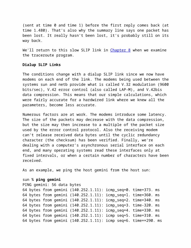
from our example in Figure 9.3) and anytime this default turns out to be wrong, it'll be informed by that default router with a redirect, allowing the host to update its routing table accordingly. ICMP redirects allow TCP/IP hosts to be dumb when it comes to routing, with all the intelligence in the routers. Obviously Rl and R2 in our example have to know more about the topology of the attached networks, but all the hosts attached to the LAN can start with a default route and learn more as they receive redirects.

An Example

We can see ICMP redirects in action on our network (inside front cover). Although we show only three hosts (aix, solaris, and gemini) and two routers (gateway and netb) on the top network, there are more than 150 hosts and 10 other routers on this network. Most of the hosts specify gateway as the default router, since it provides access to the Internet.

How is the author's subnet (the bottom four hosts in the figure) accessed from the hosts on the 140.252.1 subnet? First recall that if only a single host is at the end of the SLIP link, proxy ARP is used (Section 4.6). This means nothing special is required for hosts on the top network (140.252.1) to access the host sun (140.252.1.29). The proxy ARP software in netb handles this.

When a network is at the other end of the SLIP link, however, routing becomes involved. One solution is for every host and router to know that the router netb is the gateway for the network 140.252.13. This could be done by either a static route in each host's routing table, or by running a routing daemon in each host. A simpler way (and the method actually used) is to utilize ICMP redirects.

Let's run the ping program from the host solaris on the top network to the host bsdi (140.252.13.35) on the bottom network. Since the subnet IDs are different, proxy ARP can't be used. Assuming a static route has not been installed, the first packet sent will use the default route to the router gateway. Here is the routing table before we run ping:

solaris % netstat -rnRouting Table:

Destination Gateway Flags Ref Use Interface127.0.0.1 140.252.1.0224.0.0.0default

127.0.0.1140.252.1.32140.252.1.32140.252.1.4

UHUUUG

0330

8481504205747

lo0le0le0

(The entry for 224.0.0.0 is for IP multicasting. We describe it in Chapter 12.) If we specify the -v option to ping, we'll see any ICMP messages received by the host. We need to specify this to see the redirect message that's sent.

solaris % ping -sv bsdi PING bsdi: 56 data bytesICMP Host redirect from gateway gateway (140.252.1.4)to netb (140.252.1.183) for bsdi (140.252.13.35)64 bytes from bsdi (140.252.13.35): icmp_seq=0. time=383. Ms64 bytes from bsdi (140.252.13.35): icmp_seq=l. time=364. Ms64 bytes from bsdi (140.252.13.35): icmp_seq=2. time=353. Ms^? type interrupt key to stop --bsdi PING Statistics--4 packets transmitted, 3 packets received, 25% packet lossround-trip (ms) min/avg/max = 353/366/383

Before we receive the first ping response, the host receives an ICMP redirect from the default router gateway. If we then look at the routing table, we'll see that the new route to the host bsdi has been inserted. (This new entry is shown in a bolder font.)

Solaris % netstat -rnRouting Table:

Destination Gateway Flags Ref Use Interface 127.0.0.1 140.252.13.35140.252.1.0224.0.0.0default

127.0.0.1140.252.1.183140.252.1.32140.252.1.32140.252.1.4

UHHGHDUUUG

00330

84821504505747

lo0

le0le0

This is the first time we've seen the D flag, which means the route was installed by an ICMP redirect. The G flag means it's an indirect route to a gateway (netb), and the H flag means it's a host route (as we expect), not a network route.

Since this is a host route, added by a host redirect, it handles only the host bsdi. If we then access the host svr4, another redirect is generated, creating another host route. Similarly, accessing the host slip creates another host route. The point here is that each redirect is for a single host, causing a host route to be added. All three hosts on the author's subnet (bsdi, svr4, and slip) could also be handled by a single network route pointing to the router sun. But ICMP redirects create host routes, not network routes, because the router generating the redirect in this example (gateway) has no knowledge of the subnet structure on the 140.252.13 network.

More Details

Figure 9.4 shows the format of the ICMP redirect message.

Figure 9.4 ICMP redirect message.

There are four different redirect messages, with different code values, as shown in Figure 9.5.

code Description

0 123

redirect for networkredirect for hostredirect for type-of-service and networkredirect for type-of-service and host

Figure 9.5 Different code values for ICMP redirect.

There are three IP addresses that the receiver of an ICMP redirect must look at: (1) the IP address that caused the redirect (which is in the IP header returned as the data portion of the ICMP redirect), (2) the IP address of the router that sent the redirect (which is the source IP address of the IP datagram containing the redirect), and (3) the IP address of the router that should be used (which is in bytes 4-7 of the ICMP message).

There are numerous rules about ICMP redirects. First, redirects are generated only by routers, not by hosts. Also, redirects are intended to be used by hosts, not routers. It is assumed that routers participate in a routing protocol with other routers, and the routing protocol should obviate the need for redirects. (This means that in Figure 9.1 the routing table should be updated by either a routing daemon or redirects, but not by both.)

4.4BSD, when acting as a router, performs the following checks, all of which must be true before an ICMP redirect is generated.

1. The outgoing interface must equal the incoming interface. 2. The route being used for the outgoing datagram must not have been created or

modified by an ICMP redirect, and must not be the router's default route.

3. The datagram must not be source routed.

4. The kernel must be configured to send redirects.

The kernel variable is named ip_sendredirects, or something similar. (See Appendix E.) Most current systems (4.4BSD, SunOS 4.1.x, Solaris 2.x, and AIX 3.2.2, for example) enable this variable by default. Other systems such as SVR4 disable it by default.

Additionally, a 4.4BSD host that receives an ICMP redirect performs some checks before modifying its routing table. These are to prevent a misbehaving router or host, or a malicious user, from incorrectly modifying a system's routing table.

1. The new router must be on a directly connected network. 2. The redirect must be from the current router for that destination.

3. The redirect cannot tell the host to use itself as the router.

4. The route that's being modified must be an indirect route.

Our final point about redirects is that routers should send only host redirects (codes 1 or 3 from Figure 9.5) and not network redirects. Subnetting makes it hard to specify exactly when a network redirect can be sent instead of a host redirect. Some hosts treat a received network redirect as a host redirect, in case a router sends the wrong type.

9.6 ICMP Router Discovery Messages

We mentioned earlier in this chapter that one way to initialize a routing table is with static routes specified in configuration files. This is often used to set a default entry. A newer way is to use the ICMP router advertisement and solicitation messages.

The general concept is that after bootstrapping, a host broadcasts or multicasts a router solicitation message. One or more routers respond with a router advertisement message. Additionally, the routers periodically broadcast or multicast their router advertisements, allowing any hosts that are listening to update their routing table accordingly.

RFC 1256 [Deering 1991] specifies the format of these two ICMP messages. Figure 9.6 shows the format of the ICMP router solicitation message. Figure 9.7 shows the format of the ICMP router advertisement message sent by routers.

Figure 9.6 Format of ICMP router solicitation message.

Figure 9.7 Format of ICMP router advertisement message.

Multiple addresses can be advertised by a router in a single message. Number of addresses is the number. Address entry size is the number of 32-bit words for each router address, and is always 2. Lifetime is the number of seconds that the advertised addresses can be considered valid.

One or more pairs of an IP address and a preference then follow. The IP address must be one of the sending router's IP addresses. The preference level is a signed 32-bit integer indicating the preference of this address as a default router address, relative to other router addresses on the same subnet. Larger values imply more preferable addresses. The preference level 0x80000000 means the corresponding address, although advertised, is not to be used by the receiver as a default router address. The default value of the preference is normally 0.

Router Operation

When a router starts up it transmits periodic advertisements on all interfaces capable of broadcasting or multicasting. These advertisements are not exactly periodic, but are randomized, to reduce the probability of synchronization with other routers on the same subnet. The normal time interval between advertisements is between 450 and 600 seconds. The default lifetime for a given advertisement is 30 minutes.

Another use of the lifetime field occurs when an interface on a router is disabled. In that case the router can transmit a final advertisement on the interface with the lifetime set to 0.

In addition to the periodic, unsolicited advertisements, a router also listens for solicitations from hosts. It responds to these solicitations with a router advertisement.

If there are multiple routers on a given subnet, it is up to the system administrator to configure the preference level for each router as appropriate. For example, the primary default router would have a higher preference than a backup.

Host Operation

Upon bootstrap a host normally transmits three router solicitations, 3 seconds apart. As soon as a valid advertisement is received, the solicitations stop.

A host also listens for advertisements from adjacent routers. These advertisements can cause the host's default router to change. Also, if an advertisement is not received for the current default, that default can time out.

As long as the normal default router stays up, that router will send advertisements every 10 minutes, with a lifetime of 30 minutes. This means the host's default entry won't time out, even if one or two advertisements are lost.

Implementation

The router discovery messages are normally generated by and processed by a user process (a daemon). This adds yet another program updating the routing table in Figure 9.1, although it would only add or delete a default entry. The daemon would have to be configured to act as a router or a host.

These two ICMP messages are new and not supported by all systems. Solaris 2.x is the only system in our network that supports these messages (the in.rdisc.daemon). Although the RFC recommends using IP multicasting whenever possible, router discovery can work using broadcast messages also.

TFTP: Trivial File Transfer Protocol

15.1 Introduction

TFTP is the Trivial File Transfer Protocol. It is intended to be used when bootstrapping diskless systems (normally workstations or X terminals). Unlike the File Transfer Protocol (FTP), which we describe in Chapter 27 and which uses TCP, TFTP was designed to use UDP, to make it simple and small. Implementations of TFTP (and its required UDP, IP, and a device driver) can fit in read-only memory.

This chapter provides an overview of TFTP because we'll encounter it in the next chapter with the Bootstrap Protocol. We also encountered TFTP in Figure 5.1 when we bootstrapped the host sun from the network. It issued a TFTP request after obtaining its IP address using RARP.

RFC 1350 [Sollins 1992] is the official specification of version 2 of TFTP. Chapter 12 of [Stevens 1990] provides a complete source code implementation of a TFTP client and server, and describes some of the programming techniques used with TFTP.

15.2 Protocol

Each exchange between a client and server starts with the client asking the server to either read a file for the client or write a file for the client. In the normal case of bootstrapping a diskless system, the first request is a read request (RRQ). Figure 15.1 shows the format of the five TFTP messages. (Opcodes 1 and 2 share the same format.)

Figure 15.1 Format of the five TFTP messages.

The first 2 bytes of the TFTP message are an opcode. For a read request (RRQ) and write request (WRQ) the filename specifies the file on the server that the client wants to read from. or write to. We specifically show that this filename is terminated by a byte of 0 in Figure 15.1. The mode is one of the ASCII strings netascii or octet (in any combination of uppercase or lowercase), again terminated by a byte of 0. netascii means the data are lines

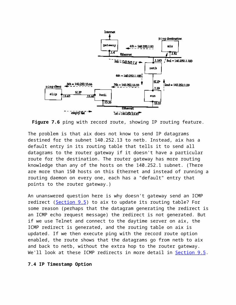
of ASCII text with each line terminated by the 2-character sequence of a carriage return followed by a linefeed (called CR/LF). Both ends must convert between this format and whatever the local host uses as a line delimiter. An octet transfer treats the data as 8-bit bytes with no interpretation.

Each data packet contains a block number that is later used in an acknowledgment packet. As an example, when reading a file the client sends a read request (RRQ) specifying the filename and mode. If the file can be read by the client, the server responds with a data packet with a block number of 1. The client sends an ACK of block number 1. The server responds with the next data packet, with a block number of 2. The client sends an ACK of block number 2. This continues until the file is transferred. Each data packet contains 512 bytes of data, except for the final packet, which contains 0-511 bytes of data. When the client receives a data packet with less than 512 bytes of data, it knows it has received the final packet.

In the case of a write request (WRQ), the client sends the WRQ specifying the filename and mode. If the file can be written by the client, the server responds with an ACK of block number 0. The client then sends the first 512 bytes of file with a block number of 1. The server responds with an ACK of block number 1.

This type of data transmission is called a stop-and-wait protocol. It is found only in simple protocols such as TFTP. We'll see in Section 20.3 that TCP provides a different form of acknowledgment, which can provide higher throughput. TFTP is designed for simplicity of implementation, not high throughput.

The final TFTP message type is the error message, with an opcode of 5. This is what the server responds with if a read request or write request can't be processed. Read and write errors during file transmission also cause this message to be sent, and transmission is then terminated. The error number gives a numeric error code, followed by an ASCII error message that might contain additional, operating system specific information.

Since TFTP uses the unreliable UDP, it is up to TFTP to handle lost and duplicated packets. Lost packets are detected with a timeout and retransmission implemented by the sender. (Be aware of a potential problem called the "sorcerer's apprentice syndrome" that can occur if both sides time out and retransmit. Section 12.2 of [Stevens 1990] shows how the problem can occur.) As with most UDP applications, there is no checksum in the TFTP messages, which assumes any corruption of the data will be caught by the UDP checksum (Section 11.3).

15.3 An Example

Let's examine TFTP by watching the protocol in action. We'll run the TFTP client on the host bsdi and fetch a text file from the host svr4:

bsdi % tftp svr4 start the TFTP client

tftp> get testl.c fetch a file from the server Received 962 bytes in 0.3 seconds tftp> quit and terminatebsdi % ls -1 testl.c how many bytes in thefile we fetched? -rw-r-r- 1 rstevens staff 914 Mar 20 11:41 test1.c bsdi % wc -1 testl.c and how many lines? 48 testl.c

The first point that catches our eye is that the file contains 914 bytes under Unix, but TFTP transfers 962 bytes. Using the wc program we see that there are 48 lines in the file, so the 48 Unix newline characters are expanded into 48 CR/LF pairs, since the TFTP default is a netascii transfer. Figure 15.2 shows the packet exchange that takes place.

1 0.0 bsdi.ll06 > svr4.tftp: 19 RRQ "testl.c" 2 3

0.287080 (0.2871)0.291178 (0.0041)

svr4.1077 > bsdi.ll06: udp 516bsdi.1106 > svr4.1077: udp 4

4 5

0.299446 (0.0083)0.312320 (0.0129)

svr4.1077 > bsdi.1106: udp 454bsdi.ll06 > svr4.1077: udp 4

Figure 15.2 Packet exchange for TFTP of a file.

Line 1 shows the read request from the client to the server. Since the destination UDP port is the TFTP well-known port (69), tcpdump interprets the TFTP packet and prints RRQ and the name of the file. The length of the UDP data is printed as 19 bytes and is accounted for as follows: 2 bytes for the opcode, 7 bytes for the filename, 1 byte of 0, 8 bytes for netascii, and another byte of 0.

The next packet is from the server (line 2) and contains 516 bytes: 2 bytes for the opcode, 2 bytes for the block number, and 512 bytes of data. Line 3 is the acknowledgment for this data: 2 bytes for the opcode and 2 bytes for the block number.

The final data packet (line 4) contains 450 bytes of data. The 512 bytes of data in line 2 and this 450 bytes of data account for the 962 bytes of data output by the client.

Note that tcpdump doesn't output any additional TFTP protocol information for lines 2-5, whereas it interpreted the TFTP message in line 1. This is because the server's port number changes between lines 1 and 2. The TFTP protocol requires that the client send the first packet (the RRQ or WRQ) to the server's well-known UDP port (69). The server then allocates some other unused ephemeral port on the server's host (1077 in Figure 15.2), which is then used by the server for all further packet exchange between this client and server. The client's port number (1106 in this example) doesn't change, tcpdump has no idea that port 1077 on host svr4 is really a TFTP server.

The reason the server's port number changes is so the server doesn't tie up the well-known port for the amount of time required to transfer the file (which could be many seconds or

even minutes). Instead, the well-known port is left available for other TFTP clients to send their requests to, while the current transfer is under way.

Recall from Figure 10.6 that when the RIP server had more than 512 bytes to send to the client, both UDP datagrams came from the server's well-known port. In that example, even though the server had to write multiple datagrams to send all the data back, the server did one write, followed by the next, both from its well-known port. Here, with TFTP, the protocol is different since there is a longer term relationship between the client and server (which we said could be seconds or minutes). If one server process used the well-known port for the duration of the file transfer, it would either have to refuse any further requests that arrived from other clients, or that one server process would have to multiplex file transfers with multiple clients at the same time, on the same port (69). The simplest solution is to have the server obtain a new port after it receives the RRQ or WRQ. Naturally the client must detect this new port when it receives the first data packet (line 2 in Figure 15.2) and then send all further acknowledgments (lines 3 and 5) to that new port. In Section 16.3 we'll see TFTP used when an X terminal is bootstrapped.

15.4 Security

Notice in the TFTP packets (Figure 15.1) that there is no provision for a username or password. This is a feature (i.e., "security hole") of TFTP. Since TFTP was designed for use during the bootstrap process it could be impossible to provide a username and password.

This feature of TFTP was used by many crackers to obtain copies of a Unix password file and then try to guess passwords. To prevent this type of access, most TFTP servers nowadays provide an option whereby only files in a specific directory (often /tftpboot on Unix systems) can be accessed. This directory then contains only the bootstrap files required by the diskless systems.

For additional security, the TFTP server on a Unix system normally sets its user ID and group ID to values that should not be assigned to any real user. This allows access only to files that have world-read or world-write permissions.

BOOTP: Bootstrap Protocol

16.1 Introduction

In Chapter 5 we described how a diskless system, with no knowledge of its IP address, can determine its IP address using RARP when it is bootstrapped. There are two problems with RARP: (1) the only thing returned is the IP address, and (2) since RARP uses a link-layer broadcast, RARP requests are not forwarded by routers (necessitating an RARP server on every physical network). This chapter describes an alternative method for a diskless system to bootstrap itself, called the Bootstrap Protocol, or BOOTP.

BOOTP uses UDP and normally works in conjunction with TFTP (Chapter 15). RFC 951 [Croft and Gilmore 1985] is the official specification for BOOTP with clarifications given in RFC 1542 [Wimer 1993].

16.2 BOOTP Packet Format

BOOTP requests and replies are encapsulated in UDP datagrams, as shown in Figure 16.1.

Figure 16.1 Encapsulation of BOOTP requests and replies within a UDP datagram.

Figure 16.2 shows the format of the 300-byte BOOTP request and reply.

Figure 16.2 Format of BOOTP request and reply.

Opcode is 1 for a request and 2 for a reply. The hardware type field is 1 for a 10 Mbits/sec Ethernet, the same value that is in the field of the same name in an ARP request or reply (Figure 4.3). Similarly, the hardware address length is 6 bytes for an Ethernet.

The hop count is set to 0 by the client, but can be used by a proxy server (described in Section 16.5).

The transaction ID is a 32-bit integer set by the client and returned by the server. This lets the client match a response with a request. The client should set this to a random number for each request.

Number of seconds can be set by the client to the time since it started trying to bootstrap. The servers can look at this value, and perhaps a secondary server for a client won't

respond until the number of seconds has exceeded some value, implying that the client's primary server is down.

If the client already knows its IP address, it fills in the client IP address. Otherwise, the client sets this to 0. In the latter case the server fills in your IP address with the client's IP address. The server IP address is filled in by the server. If a proxy server is used (Section 16.5), that proxy server fills in its gateway IP address.

The client must set its client hardware address. Although this is the same value as in the Ethernet header, by placing the field in the UDP datagram also, it is easily available to any user process (e.g., a BOOTP server) that receives the datagram. It is normally much harder (or impossible) for a process reading UDP datagrams to determine the fields in the Ethernet header that carried the UDP datagram.

The server hostname is a null terminated string that is optionally filled in by the server. The server can also fill in the boot filename with the fully qualified, null terminated pathname of a file to bootstrap from.

The vendor-specific area is used for various extensions to BOOTP. Section 16.6 describes some of these extensions.

When a client is bootstrapping using BOOTP (an opcode of 1) the request is normally a link-layer broadcast and the destination IP address in the IP header is normally 255.255.255.255 (the limited broadcast. Section 12.2). The source IP address is often 0.0.0.0 since the client does not know its own IP address yet. Recall from Figure 3.9 that 0.0.0.0 is a valid source IP address when a system is bootstrapping itself.

Port Numbers

There are two well-known ports for BOOTP: 67 for the server and 68 for the client. This means the client does not choose an unused ephemeral port, but uses 68 instead. The reason two port numbers were chosen, instead of just one for the server, is that a server's reply can be (but normally isn't) broadcast.

If the server's reply were broadcast, and if the client were to choose an ephemeral port number, these broadcasts would also be received by other applications on other hosts that happen to be using the same ephemeral port number. Hence, it is considered bad form to broadcast to a random (i.e., ephemeral) port number.

If the client also used the server's well-known port (67) as its port, then all servers on the network are awakened to look at each broadcast reply. (If all the servers were awakened, they would examine the opcode, see that it's a reply and not a request, and go back to sleep.) Therefore the choice was made to have all clients use a single well-known port that differs from the server's well-known port.

If multiple clients are bootstrapping at the same time, and if the server broadcasts the replies, each client sees the replies intended for the other clients. The clients can use the transaction ID field in the BOOTP header to match replies with requests, or the client can examine the returned client hardware address.

16.3 An Example

Let's look at an example of BOOTP when an X terminal is bootstrapped. Figure 16.3 shows the tcpdump output. (The client's name is proteus and the server's name is mercury. This tcpdump output was obtained on a different network from the one we've been using for all the other examples in the text.)

1 0.0 0.0.0.0.68 > 255.255.255.255.bootp: secs: 100 ether 0:0:a7:0:62:7c

2 0.355446 (0.3554) mercury.bootp > proteus.68: secs:100 Y:proteus S: mercury G: mercury ether 0:0:a7:0:62:7cfile "/local/var/bootfiles/Xncdl9r"

3 0.355447 (0.0000) arp who-has proteus tell 0.0.0.04 0.851508 (0.4961) arp who-has proteus tell 0.0.0.05 1.371070 (0..5196) arp who-has proteus tell proteus

6 1.863226 (0..4922) proteus.68 > 255.255.255.255.bootp: secs: 100 ether 0:0:a7:0:62:7c

7 1.71038 (0..0078) mercury.bootp > proteus.68: secsilOO Y:proteus S: mercury G: mercury ether 0:0:a7:0;62:7cfile "/local/var/bootfiles/Xncdl9r"

8 3.871038 (2.0000) proteus.68 > 255.255.255.255.bootp:secs: 1OO ether 0:0:a7:0:62:7c

9 3.878850 (0.0078) mercury.bootp > proteus. 68: secs: 100 Y:proteus S: mercury G: mercury ether 0:0:a7:0:62:7cfile "/local/var/bootfiles/Xncdl9r"

10 5.925786 (2.0469) arp who-has mercury tell proteus11 5.929692 (0.0039) arp reply mercury is-at 8:0:2b:28:eb:1d

12 5.929694 (0.0000) proteus. tftp > mercury, tftp: 37 RRQ "/local/var/bootfiles/Xncdl9r"

13 5.996094 (0.0664) mercury.2352 > proteus.tftp: 516 DATA block 1 14 6.000000 (0.0039) proteus. tftp > mercury. 2352: 4 ACK

many lines deleted here 15 14.980472 (8.9805) mercury.2352 > proteus.tftp: 516 DATA block 2510 16 14.984376 (0.0039) proteus. tftp > mercury. 2352: 4 ACK 17 14.984377 (0.0000) mercury. 2352 > proteus. tftp: 228 DATA block 2464 18 14.984378 (0.0000) proteus.tftp > mercury.2352: 4 ACK

Figure 16.3 Example of BOOTP being used to bootstrap an X terminal.

In line 1 we see the client's request from 0.0.0.0.68, destined for 255.255.255.255.67. The only fields the client has filled in are the number of seconds and its Ethernet address. We'll see that this client always sets the number of seconds to 100. The hop count and transaction ID are both 0 since they are not output by tcpdump. (A transaction ID of 0 means the client ignores the field, since it would set this field to a random number if it was going to verify the returned value in the response.)

Line 2 is the reply from the server. The fields filled in by the server are the client's IP address (which tcpdump prints as the name proteus), the server's IP address (printed as the name mercury), the IP address of a gateway (printed as the name mercury), and the name of a boot file.

After receiving the BOOTP reply, the client immediately issues an ARP request to see if anyone else on the network has its IP address. The name proteus following who-has corresponds to the target IP address (Figure 4.3), and the sender's IP address is set to 0.0.0.0. It sends another identical ARP request 0.5 second later, and another one 0.5 second after that. In the third ARP request (line 5) it changes the sender's IP address to be its own IP address. This is a gratuitous ARP request (Section 4.7).

Line 6 shows that the client waits another 0.5 second and broadcasts another BOOTP request. The only difference between this request and line 1 is that now the client puts its own IP address in the IP header. It receives the same reply from the same server (line 7). The client waits another 2 seconds and broadcasts yet another BOOTP request (line 8) and receives the same reply from the same server.

The client then waits another 2 seconds and sends an ARP request for its server mercury (line 10). The ARP reply is received and the client immediately issues a TFTP read request for its boot file (line 12). What follows are 2464 TFTP data packets and acknowledgments. The amount of data transferred is 512 x 2463+224 = 1,261,280 bytes. This loads the operating system into the X terminal. We have deleted most of the TFTP lines from Figure 16.3.

One thing to notice, when comparing this TFTP exchange with Figure 15.2, is that here the client uses the TFTP well-known port (69) for the entire transfer. Since one of the two partners is using port 69, tcpdump knows that the packets are TFTP messages, so it is able to interpret each packet using the TFTP protocol. This is why Figure 16.3 indicates which packets contain data, which contain acknowledgments, and what the block number is for each packet. We didn't get this additional information in Figure 15.2 because neither end was using TFTP's well-known port for the data transfer. Normally the TFTP client cannot use TFTP's well-known port, since that port is used by the server on a multiuser system. But here the system is being bootstrapped, so a TFTP server is not provided, allowing the client to use the port for the duration of the transfer. This also implies that the TFTP server on mercury doesn't care what the client's port number is-it sends the data to the client's port, whatever that happens to be.

From Figure 16.3 we see that 1,261,280 bytes are transferred in 9 seconds. This is a rate of about 140,000 bytes per second. While this is slower than most FTP file transfers across an Ethernet, it is not that bad for a simple stop-and-wait protocol such as TFTP.

What follows as this X terminal is bootstrapped are additional TFTP transfers of the terminal's font files, some DNS name server queries, and then the initialization of the X protocol. The total time in Figure 16.3 was almost 15 seconds, and another 6 seconds is taken for the remaining steps. This gives a total of 21 seconds to bootstrap the diskless X terminal.

16.4 BOOTP Server Design

The BOOTP client is normally provided in read-only memory on the diskless system. It is interesting to see how the server is normally implemented.

First, the server reads UDP datagrams from its well-known port (67). Nothing special is required. This differs from an RARP server (Section 5.4), which we said had to read Ethernet frames with a type field of "RARP request." The BOOTP protocol also made it easy for the server to obtain the client's hardware address, by placing it into the BOOTP packet (Figure 16.2).

An interesting problem arises: how can the server send a response directly back to the client? The response is a UDP datagram, and the server knows the client's IP address (probably read from a configuration file on the server). But if the client sends a UDP datagram to that IP address (the normal way UDP output is handled), the server's host will probably issue an ARP request for that IP address. But the client can't respond to the ARP request since it doesn't know its IP address yet! (This is called the "chicken and egg" issue in RFC 951.)

There are two solutions. The first, commonly used by Unix servers, is tor the server to issue an ioctl(2) request to the kernel, to place an entry into the ARP cache for this client. (This is what the arp -s command does. Section 4.8.) The server can do this since it knows the client's hardware address and IP address. This means that when the server sends the UDP datagram (the BOOTP reply), the server's ARP module will find the client's IP address in the ARP cache.

An alternative solution is tor the server to broadcast the BOOTP reply, instead of sending it directly to the client. Since reducing the number of broadcasts on a network is always desirable, this solution should be used only if the server cannot make an entry into its ARP cache. Normally it requires superuser permission to make an entry into the ARP cache, requiring a broadcast reply if the server is nonprivileged.

16.5 BOOTP Through a Router

We said in Section 5.4 that one of the drawbacks of RARP is that it uses a link-layer broadcast, which is normally not forwarded by a router. This required an RARP server on

each physical network. BOOTP can be used through a router, if supported by the router. (Most major router vendors do support this feature.)

This is mainly intended for diskless routers, because if a multiuser system with a disk is used as a router, it can probably run a BOOTP server itself. Alternatively, the common Unix BOOTP server (Appendix F) supports this relay mode, but again, if you can run a BOOTP server on the physical network, there's normally no need to forward the requests to yet another server on another network.

What happens is that the router (also called the "BOOTP relay agent") listens tor BOOTP requests on the server's well-known port (67). When a request is received, the relay agent places its IP address into the gateway IP address field in the BOOTP request, and sends the request to the real BOOTP server. (The address placed by the relay agent into the gateway field is the IP address of the interface on which the request was received.) The relay agent also increments the hops field by one. (This is to prevent infinite loops in case the request is reforwarded. RFC 951 mentions that the request should probably be thrown away if the hop count reaches 3.) Since the outgoing request is a unicast datagram (as opposed to the original client request that was broadcast), it can follow any route to the real BOOTP server, passing through other routers. The real server gets the request, forms the BOOTP reply, and sends it back to the relay agent, not the client. The real server knows that the request has been forwarded, since the gateway field in the request is nonzero. The relay agent receives the reply and sends it to the client.

16.6 Vendor-Specific Information

In Figure 16.2 we showed a 64-byte vendor-specific area, RFC 1533 [Alexander and Droms 1993] defines the format of this area. This area contains optional information for the server to return to the client.

If information is provided, the first 4 bytes of this area are set to the IP address 99.130.83.99. This is called the magic cookie and means there is information in the area.

The rest of this area is a list of items. Each item begins with a 1-byte tag field. Two of the items consist of just the tag field: a tag of 0 is a pad byte (to force following items to preferred byte boundaries), and a tag of 255 marks the end of the items. Any bytes remaining in this area after the first end byte should be set to this value (255).

Other than these two 1-byte items, the remaining items consist of a single length byte, followed by the information. Figure 16.4 shows the format of some of the items in the vendor-specific area.

Figure 16.4 Format of some of the items in the vendor-specific area.

The subnet mask and time value are really fixed-length items because their values always occupy 4 bytes. The time offset is the number of seconds since midnight January 1,1900, UTC.

The gateway item is an example of a variable-length item. The length is always a multiple of 4, and the values are the 32-bit IP addresses of one or more gateways (routers) for the client to use. The first one returned must be the preferred gateway.

There are 14 other items defined in RFC 1533. Probably the most important is the IP address of a DNS name server, with a tag value of 6. Other items return the IP address of a printer server, the IP address of a time server, and so on. Refer to the RFC for all the details.

Returning to our example in Figure 16.3, we never saw an ICMP address mask request (Section 6.3) that would have been broadcast by the client to find its subnet mask. Although it wasn't output by tcpdump, we can probably assume that the client's subnet mask was returned in the vendor-specific area of the BOOTP reply.

The Host Requirements RFC recommends that a system using BOOTP obtain its subnet mask using BOOTP, not ICMP.

The size of the vendor-specific area is limited to 64 bytes. This is a constraint for some applications. A new protocol named DHCP (Dynamic Host Configuration Protocol) is built on, but replaces, BOOTP. DHCP extends this area to 312 bytes and is defined in RFC 1541 [Droms 1993].

UNIT-IV

TCP Connection Establishment and Termination

18.1 Introduction

TCP is a connection-oriented protocol. Before either end can send data to the other, a connection must be established between them. In this chapter we take a detailed look at how a TCP connection is established and later terminated.

This establishment of a connection between the two ends differs from a connectionless protocol such as UDP. We saw in Chapter 11 that with UDP one end just sends a datagram to the other end, without any preliminary handshaking.

18.2 Connection Establishment and Termination

To see what happens when a TCP connection is established and then terminated, we type the following command on the system svr4:

svr4 % telnet bsdi discard Trying 192.82.148.3 ...Connected to bsdi.Escape character is '^]'.^] type Control, right bracket to talk to the Telnet client telnet> quit terminate the connection Connection closed.

The telnet command establishes a TCP connection with the host bsdi on the port corresponding to the discard service (Section 1.12). This is exactly the type of service we need to see what happens when a connection is established and terminated, without having the server initiate any data exchange.

tcpdump Output

Figure 18.1 shows the tcpdump output for the segments generated by this command.

1 0.0 svr4.1037 > bsdi.discard: S 1415531521:1415531521(0) win 4096 <mss 1024>

2 0.002402 (0.0024) bsdi.discard > svr4.1037: S 1823083521:1823083521(0) ack 1415531522 win 4096 <mss 1024>

3 0.007224 (0.0048) svr4.1037 > bsdi.discard: ack 1823083522 win 4096

4 4.155441 (4.1482) svr4.1037 > bsdi.discard: F 1415531522:1415531522(0) ack 1823083522 win 4096

5 4.156747 (0.0013) bsdi.discard > svr4.1037: . ack 1415531523 win 4096

6 4.158144 (0.0014) bsdi.discard > svr4.1037: F 1823083522:1823083522(0) ack 1415531523 win 4096

7 4.180662 (0.0225) svr4.1037 > bsdi.discard: . ack 1823083523 win 4096 Figure 18.1 tcpdump output for TCP connection establishment and termination.

These seven TCP segments contain TCP headers only. No data is exchanged. For TCP segments, each output line begins with

source > destination: flags

where flags represents four of the six flag bits in the TCP header (Figure 17.2). Figure 18.2 shows the five different characters that can appear in the flags output.

flag3-character

abbreviationDescription

SFRP.

SYNFINRSTPSH

-

synchronize sequence numberssender is finished sending datareset connectionpush data to receiving process as soon as possiblenone of above four flags is on

Figure 18.2 flag characters output by tcpdump for flag bits in TCP header.

In this example we see the S, F, and period. We'll see the other two flags (R and P) later. The other two TCP header flag bits-ACK and URG-are printed specially by tcpdump.

It's possible for more than one of the four flag bits in Figure 18.2 to be on in a single segment, but we normally see only one on at a time.

RFC 1025 [Postel 1987], the TCP and IP Bake Off, calls a segment with the maximum combination of allowable flag bits turned on at once (SYN, URG, PSH, FIN, and 1 byte of data) a Kamikaze packet. It's also known as a nastygram, Christmas tree packet, and lamp test segment.

In line 1, the field 1415531521:1415531521 (0) means the sequence number of the packet was 1415531521 and the number of data bytes in the segment was 0. tcpdump displays this by printing the starting sequence number, a colon, the implied ending sequence number, and the number of data bytes in parentheses. The advantage of displaying both the sequence number and the implied ending sequence number is to see what the implied ending sequence number is, when the number of bytes is greater than 0. This field is output only if (1) the segment contains one or more bytes of data or (2) the SYN, FIN, or RST flag

was on. Lines 1, 2, 4, and 6 in Figure 18.1 display this field because of the flag bits-we never exchange any data in this example.

In line 2 the field ack 1415531522 shows the acknowledgment number. This is printed only if the ACK flag in the header is on.

The field win 4096 in every line of output shows the window size being advertised by the sender. In these examples, where we are not exchanging any data, the window size never changes from its default of 4096. (We examine TCP's window size in Section 20.4.)

The final field that is output in Figure 18.1, <mss 1024> shows the maximum segment size (MSS) option specified by the sender. The sender does not want to receive TCP segments larger than this value. This is normally to avoid fragmentation (Section 11.5). We discuss the maximum segment size in Section 18.4, and show the format of the various TCP options in Section 18.10.

Time Line

Figure 18.3 shows the time line for this sequence of packets. (We described some general features of these time lines when we showed the first one in Figure 6.11.) This figure shows which end is sending packets. We also expand some of the tcpdump output (e.g., printing SYN instead of S). In this time line we have also removed the window size values, since they add nothing to the discussion.

Connection Establishment Protocol

Now let's return to the details of the TCP protocol that are shown in Figure 18.3. To establish a TCP connection:

1. The requesting end (normally called the client) sends a SYN segment specifying the port number of the server that the client wants to connect to, and the client's initial sequence number (ISN, 1415531521 in this example). This is segment 1.

2. The server responds with its own SYN segment containing the server's initial sequence number (segment 2). The server also acknowledges the client's SYN by ACKing the client's ISN plus one. A SYN consumes one sequence number.

3. The client must acknowledge this SYN from the server by ACKing the server's ISN plus one (segment 3).

These three segments complete the connection establishment. This is often called the three-way handshake.

Figure 18.3 Time line of connection establishment and connection termination.

The side that sends the first SYN is said to perform an active open. The other side, which receives this SYN and sends the next SYN, performs a passive open. (In Section 18.8 we describe a simultaneous open where both sides can do an active open.)

When each end sends its SYN to establish the connection, it chooses an initial sequence number for that connection. The ISN should change over time, so that each connection has a different ISN. RFC 793 [Postel 1981c] specifies that the ISN should be viewed as a 32-bit counter that increments by one every 4 microseconds. The purpose in these sequence numbers is to prevent packets that get delayed in the network from being delivered later and then misinterpreted as part of an existing connection.

How are the sequence numbers chosen? In 4.4BSD (and most Berkeley-derived implementations) when the system is initialized the initial send sequence number is initialized to 1. This practice violates the Host Requirements RFC. (A comment in the code acknowledges that this is wrong.) This variable is then incremented by 64,000 every half-second, and will cycle back to 0 about every 9.5 hours. (This corresponds to a counter that is incremented every 8 microseconds, not every 4 microseconds.) Additionally, each time a connection is established, this variable is incremented by 64,000.

The 4.1-second gap between segments 3 and 4 is the time between establishing the connection and typing the quit command to telnet to terminate the connection.

Connection Termination Protocol

While it takes three segments to establish a connection, it takes four to terminate a connection. This is caused by TCP's half-close. Since a TCP connection is full-duplex (that is, data can be flowing in each direction independently of the other direction), each direction must be shut down independently. The rule is that either end can send a FIN when it is done sending data. When a TCP receives a FIN, it must notify the application that the other end has terminated that direction of data flow. The sending of a FIN is normally the result of the application issuing a close.

The receipt of a FIN only means there will be no more data flowing in that direction. A TCP can still send data after receiving a FIN. While it's possible for an application to take advantage of this half-close, in practice few TCP applications use it. The normal scenario is what we show in Figure 18.3. We describe the half-close in more detail in Section 18.5.

We say that the end that first issues the close (e.g., sends the first FIN) performs the active close and the other end (that receives this FIN) performs the passive close. Normally one end does the active close and the other does the passive close, but we'll see in Section 18.9 how both ends can do an active close.

Segment 4 in Figure 18.3 initiates the termination of the connection and is sent when the Telnet client closes its connection. This happens when we type quit. This causes the client TCP to send a FIN, closing the flow of data from the client to the server.

When the server receives the FIN it sends back an ACK of the received sequence number plus one (segment 5). A FIN consumes a sequence number, just like a SYN. At this point the server's TCP also delivers an end-of-file to the application (the discard server). The server then closes its connection, causing its TCP to send a FIN (segment 6), which the client TCP must ACK by incrementing the received sequence number by one (segment 7).

Figure 18.4 shows the typical sequence of segments that we've described for the termination of a connection. We omit the sequence numbers. In this figure sending the FINs is caused by the applications closing their end of the connection, whereas the ACKs of these FINs are automatically generated by the TCP software.

Connections are normally initiated by the client, with the first SYN going from the client to the server. Either end can actively close the connection (i.e., send the first FIN). Often, however, it is the client that determines when the connection should be terminated, since client processes are often driven by an interactive user, who enters something like "quit" to terminate. In Figure 18.4 we can switch the labels at the top, calling the left side the server and the right side the client, and everything still works fine as shown. (The first example in Section 14.4, for example, shows the daytime server closing the connection.)

Figure 18.4 Normal exchange of segments during connection termination.

Normal tcpdump Output

Having to sort through all the huge sequence numbers is cumbersome, so the default tcpdump output shows the complete sequence numbers only on the SYN segments, and shows all following sequence numbers as relative offsets from the original sequence numbers. (To generate the output for Figure 18.1 we had to specify the -S option.) The normal tcpdump output corresponding to Figure 18.1 is shown in Figure 18.5.

1 0.0 svr4.1037 > bsdi.discard: S 1415531521:1415531521(0) win 4096 <mss 1024>

2 0.002402 (0.0024) bsdi.discard > svr4.1037: S 1823083521:1823083521(0) ack 1415531522 win 4096 <mss 1024>

3 0.007224 (0.0048) svr4.1037 > bsdi.discard: . ack 1 win 4096 4 4.155441 (4.1482) svr4.1037 > bsdi.discard: F 1:1(0) ack 1 win 4096 5 4.156747 (0.0013) bsdi.discard > svr4.1037: . ack 2 win 4096 6 4.158144 (0.0014) bsdi.discard > svr4.1037: F 1:1(0) ack 2 win 4096 7 4.180662 (0.0225) svr4.1037 > bsdi.discard: . ack 2 win 4096

Figure 18.5 Normal tcpdump output for connection establishment and termination.

Unless we need to show the complete sequence numbers, we'll use this form of output in all following examples.

TCP Interactive Data Flow

19.1 Introduction

The previous chapter dealt with the establishment and termination of TCP connections. We now examine the transfer of data using TCP.

Studies of TCP traffic, such as [Caceres et al. 1991], usually find that on a packet-count basis about half of all TCP segments contain bulk data (FTP, electronic mail, Usenet news) and the other half contain interactive data (Telnet and Rlogin, for example). On a byte-count basis the ratio is around 90% bulk data and 10% interactive, since bulk data segments tend to be full sized (normally 512 bytes of user data), while interactive data tends to be much smaller. (The above-mentioned study found that 90% of Telnet and Rlogin packets carry less than 10 bytes of user data.)

TCP obviously handles both types of data, but different algorithms come into play for each. In this chapter we'll look at interactive data transfer, using the Rlogin application. We'll see how delayed acknowledgments work and how the Nagle algorithm reduces the number of

small packets across wide area networks. The same algorithms apply to Telnet. In the next chapter we'll look at bulk data transfer.

19.2 Interactive Input

Let's look at the flow of data when we type an interactive command on an Rlogin connection. Many newcomers to TCP/IP are surprised to find that each interactive keystroke normally generates a data packet. That is, the keystrokes are sent from the client to the server 1 byte at a time (not one line at a time). Furthermore, Rlogin has the remote system (the server) echo the characters that we (the client) type. This could generate four segments: (1) the interactive keystroke from the client, (2) an acknowledgment of the keystroke from the server, (3) the echo of the keystroke from the server, and (4) an acknowledgment of the echo from the client. Figure 19.1 shows this flow of data.

Figure 19.1 One possible way to do remote echo of interactive keystroke.

Normally, however, segments 2 and 3 are combined-the acknowledgment of the keystroke is sent along with the echo. We describe the technique that combines these (called delayed acknowledgments) in the next section.

We purposely use Rlogin for the examples in this chapter because it always sends one character at a time from the client to the server. When we describe Telnet in Chapter 26, we'll see that it has an option that allows lines of input to be sent from the client to the server, which reduces the network load.

Figure 19.2 shows the flow of data when we type the five characters date\n. (We do not show the connection establishment and we have removed all the type-of-service output. BSD/386 sets the TOS for an Rlogin connection for minimum delay.) Line 1 sends the character d from the client to the server. Line 2 is the acknowledgment of this character and its echo. (This is combining the middle two segments in Figure 19.1.) Line 3 is the acknowledgment of the echoed character. Lines 4-6 correspond to the character a, lines 7-9 to the character t, and lines 10-12 to the character e. The fractional second delays between lines 3-4, 6-7, 9-10, and 12-13 are the human delays between typing each character.

Notice that lines 13-15 are slightly different. One character is sent from the client to the server (the Unix newline character, from our typing the RETURN key) but two characters are echoed. These two characters are a carriage return and linefeed (CR/LF), to move the cursor back to the left and space down one line.

Line 16 is the output of the date command from the server. The 30 bytes are composed of the following 28 characters

Sat Feb 6 07:52:17 MST 1993 1 0.0 bsdi.1023 > svr4.login: P 0:1(1) ack 1 win 4096 2 0.016497 (0.0165) svr4.login > bsdi.1023: P 1:2(1) ack 1 win 4096 3 0.139955 (0.1235) bsdi.1023 > svr4.login: . ack 2 win 4096 4 0.458037 (0.3181) bsdi.1023 > svr4.login: P 1:2(1) ack 2 win 4096 5 0.474386 (0.0163) svr4.login > bsdi.1023: P 2:3(1) ack 2 win 4096 6 0.539943 (0.0656) bsdi.1023 > svr4.login: . ack 3 win 4096 7 0.814582 (0.2746) bsdi.1023 > svr4.login: P 2:3(1) ack 3 win 4096 8 0.831108 (0.0165) svr4.login > bsdi.1023: P 3:4(1) ack 3 win 4096 9 0.940112 (0.1090) bsdi.1023 > svr4.login: . ack 4 win 4096 10 1.191287 (0.2512) bsdi.1023 > svr4.login: P 3:4(1) ack 4 win 4096 11 1.207701 (0.0164) svr4.login > bsdi.1023: P 4:5(1) ack 4 win 4096 12 1.339994 (0.1323) bsdi.1023 > svr4.login: . ack 5 win 4096 13 1.680646 (0.3407) bsdi.1023 > svr4.login: P 4:5(1) ack 5 win 4096 14 1.697977 (0.0173) svr4.login > bsdi.1023: P 5:7(2) ack 5 win 4096 15 1.739974 (0.0420) bsdi.1023 > svr4.login: . ack 7 win 4096 16 1.799841 (0.0599) svr4.login > bsdi.1023: P 7:37(30) ack 5 win 4096 17 1.940176 (0.1403) bsdi.1023 > svr4.login: . ack 37 win 4096 18 1.944338 (0.0042) svr4.login > bsdi.1023: P 37:44(7) ack 5 win 4096 19 2.140110 (0.1958) bsdi.1023 > svr4.login: . ack 44 win 4096

Figure 19.2 TCP segments when date typed on Rlogin connection.

plus a CR/LF pair at the end. The next 7 bytes sent from the server to the client (line 18) are the client's prompt on the server host: svr4 % . Line 19 acknowledges these 7 bytes.

Notice how the TCP acknowledgments operate. Line 1 sends the data byte with the sequence number 0. Line 2 ACKs this by setting the acknowledgment sequence number to 1, the sequence number of the last successfully received byte plus one. (This is also called the sequence number of the next expected byte.) Line 2 also sends the data byte with a sequence number of 1 from the server to the client. This is ACKed by the client in line 3 by setting the acknowledged sequence number to 2.

19.3 Delayed Acknowledgments

There are some subtle points in Figure 19.2 dealing with timing that we'll cover in this section. Figure 19.3 shows the time line for the exchange in Figure 19.2. (We have deleted

all the window advertisements from this time line, and have added a notation indicating what data is being transferred.)

We have labeled the seven ACKs sent from bsdi to svr4 as delayed ACKs. Normally TCP does not send an ACK the instant it receives data. Instead, it delays the ACK, hoping to have data going in the same direction as the ACK, so the ACK can be sent along with the data. (This is sometimes called having the ACK piggyback with the data.) Most implementations use a 200-ms delay-that is, TCP will delay an ACK up to 200 ms to see if there is data to send with the ACK.

Figure 19.3 Time line of data flow for date command typed on an rlogin connection.

If we look at the time differences between bsdi receiving the data and sending the ACK, they appear to be random: 123.5, 65.6, 109.0, 132.3,42.0, 140.3, and 195.8 ms. Look instead at the actual times (starting from 0) when the ACKs are sent: 139.9, 539.9, 940.1, 1339.9, 1739.9, 1940.1, and 2140.1 ms. (We have marked these with an asterisk to the left of the time in Figure 19.3.) There is a multiple of 200 ms between these times. What is happening here is that TCP has a timer that goes off every 200 ms, but it goes off at fixed points in time-every 200 ms relative to when the kernel was bootstrapped. Since the data being acknowledged arrives randomly (at times 16.4, 474.3, 831.1, etc.), TCP asks to be notified the next time the kernel's 200-ms timer expires. This can be anywhere from 1 to 200 ms in the future.

If we look at how long it takes svr4 to generate the echo of each character it receives, the times are 16.5, 16.3, 16.5, 16.4, and 17.3 ms. Since this time is less than 200 ms, we never see a delayed ACK on that side. There is always data ready to be sent before the delayed ACK timer expires. (We could still see a delayed ACK if the wait period, about 16 ms, crosses one of the kernel's 200-ms clock tick boundaries. We just don't see any of these in this example.)

We saw this same scenario in Figure 18.7 with the 500-ms TCP timer used when detecting a timeout. Both TCP timers, the 200- and 500-ms timers, go off at times relative to when the kernel was bootstrapped. Whenever TCP sets a timer, it can go off anywhere between 1-200 or 1-500 ms in the future.

The Host Requirements RFC states that TCP should implement a delayed ACK but the delay must be less than 500 ms.

19.4 Nagle Algorithm

We saw in the previous section that 1 byte at a time normally flows from the client to the server across an Rlogin connection. This generates 41-byte packets: 20 bytes for the IP header, 20 bytes for the TCP header, and 1 byte of data. These small packets (called tinygrams) are normally not a problem on LANs, since most LANs are not congested, but

these tinygrams can add to congestion on wide area networks. A simple and elegant solution was proposed in RFC 896 [Nagle 1984], called the Nagle algorithm.

This algorithm says that a TCP connection can have only one outstanding small segment that has not yet been acknowledged. No additional small segments can be sent until the acknowledgment is received. Instead, small amounts of data are collected by TCP and sent in a single segment when the acknowledgment arrives. The beauty of this algorithm is that it is self-clocking: the faster the ACKs come back, the faster the data is sent. But on a slow WAN, where it is desired to reduce the number of tinygrams, fewer segments are sent. (We'll see in Section 22.3 that the definition of "small" is less than the segment size.)

We saw in Figure 19.3 that the round-trip time on an Ethernet for a single byte to be sent, acknowledged, and echoed averaged around 16 ms. To generate data faster than this we would have to be typing more than 60 characters per second. This means we rarely encounter this algorithm when sending data between two hosts on a LAN.

Things change, however, when the round-trip tune (RTT) increases, typically across a WAN. Let's look at an Rlogin connection between our host slip and the host vangogh.cs.berkeley.edu. To get out of our network (see inside front cover), two SLIP links must be traversed, and then the Internet is used. We expect much longer round-trip times. Figure 19.4 shows the time line of some data flow while characters were being typed quickly on the client (similar to a fast typist). (We have removed the type-of-service information, but have left in the window size advertisements.)

Figure 19.4 Dataflow using rlogin between slip and vangogh.cs.berkeley.edu.

The first thing we notice, comparing Figure 19.4 with Figure 19.3, is the lack of delayed ACKs from slip to vangogh. This is because there is always data ready to send before the delayed ACK timer expires.

Next, notice the various amounts of data being sent from the left to the right: 1, 1, 2, 1, 2, 2, 3, 1, and 3 bytes. This is because the client is collecting the data to send, but doesn't send it until the previously sent data has been acknowledged. By using the Nagle algorithm only nine segments were used to send 16 bytes, instead of 16 segments.

Segments 14 and 15 appear to contradict the Nagle algorithm, but we need to look at the sequence numbers to see what's really happening. Segment 14 is in response to the ACK received in segment 12, since the acknowledged sequence number is 54. But before this data segment is sent by the client, segment 13 arrives from the server. Segment 15 contains the ACK of segment 13, sequence number 56. So the client is obeying the Nagle algorithm, even though we see two back-to-back data segments from the client to the server.

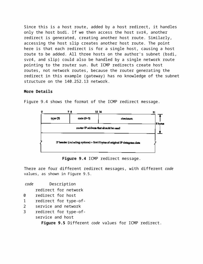
Also notice in Figure 19.4 that one delayed ACK is present, but it's from the server to the client (segment 12). We are assuming this is a delayed ACK since it contains no data. The server must have been busy at this time, so that the Rlogin server was not able to echo the character before the server's delayed ACK timer expired.

Finally, look at the amounts of data and the sequence numbers in the final two segments. The client sends 3 bytes of data (numbered 18, 19, and 20), then the server acknowledges these 3 bytes (the ACK of 21 in the final segment) but sends back only 1 byte (numbered 59). What's happening here is that the server's TCP is acknowledging the 3 bytes of data once it has received them correctly, but it won't have the echo of these 3 bytes ready to send back until the Rlogin server sends them. This shows that TCP can acknowledge received data before the application has read and processed that data. The TCP acknowledgment just means TCP has correctly received the data. We also have an indication that the server process has not read these 3 bytes of data because the advertised window in the final segment is 8189, not 8192.

Disabling the Nagle Algorithm

There are times when the Nagle algorithm needs to be turned off. The classic example is the X Window System server (Section 30.5): small messages (mouse movements) must be delivered without delay to provide real-time feedback for interactive users doing certain operations.

Here we'll show another example that's easier to demonstrate-typing one of the terminal's special function keys during an interactive login. The function keys normally generate multiple bytes of data, often beginning with the ASCII escape character. If TCP gets the data 1 byte at a time, it's possible for it to send the first byte (the ASCII ESC) and then hold the remaining bytes of the sequence waiting for the ACK of this byte. But when the server receives this first byte it doesn't generate an echo until the remaining bytes are received. This often triggers the delayed ACK algorithm on the server, meaning that the remaining bytes aren't sent for up to 200 ms. This can lead to noticeable delays to the interactive user.

The sockets API uses the TCP_NODELAY socket option to disable the Nagle algorithm.

The Host Requirements RFC states that TCP should implement the Nagle algorithm but there must be a way for an application to disable it on an individual connection.

An Example

We can see this interaction between the Nagle algorithm and keystrokes that generate multiple bytes. We establish an Rlogin connection from our host slip to the host vangogh.cs.berkeley.edu. We then type the Fl function key, which generates 3 bytes: an escape, a left bracket, and an M. We then type the F2 function key, which generates another 3 bytes. Figure 19.5 shows the tcpdump output. (We have removed the type-of-service information and the window advertisements.)

type Fl key 1 0.0 slip.1023 > vangogh. login: P 1:2(1) ack 2 2 0.250520 (0.2505) vangogh.login > slip.1023: P 2:4(2) ack 2 3 0.251709 (0.0012) slip.1023 > vangogh.login: P 2:4(2) ack 4 4 0.490344 (0.2386) vangogh.login > slip.1023: P 4:6(2) ack 4 5 0.588694 (0.0984) slip.1023 > vangogh.login: . ack 6

type F2 key 6 2.836830 (2.2481) slip.1023 > vangogh.login: P 4:5(1) ack 6 7 3.132388 (0.2956) vangogh.login > slip.1023: P 6:8(2) ack 5 8 3.133573 (0.0012) slip.1023 > vangogh.login: P 5:7(2) ack 8 9 3.370346 (0.2368) vangogh.login > slip.1023: P 8:10(2) ack 7 10 3.388692 (0.0183) slip.1023 > vangogh.login: . ack 10

Figure 19.5 Watching the Nagle algorithm when typing characters that generate multiple bytes of data.

Figure 19.6 shows the time line for this exchange. At the bottom of this figure we show the 6 bytes going from the client to the server with their sequence numbers, and the 8 bytes of echo being returned.

When the first byte of input is read by the rlogin client and written to TCP, it is sent by itself as segment 1. This is the first of the 3 bytes generated by the Fl key. Its echo is returned in segment 2, and only then are the next 2 bytes sent (segment 3). The echo of the second 2 bytes is received in segment 4 and acknowledged in segment 5.

The reason the echo of the first byte occupies 2 bytes (segment 2) is because the ASCII escape character is echoed as 2 bytes: a caret and a left bracket. The next 2 bytes of input, a left bracket and an M, are echoed as themselves.

The same exchange occurs when the next special function key is typed (segments 6-10). As we expect, the time difference between segments 5 and 10 (slip sending the acknowledgment of the echo) is a multiple of 200 ms, since both ACKs are delayed.

Figure 19.6 Time line for Figure 19.5 (watching the Nagle algorithm).

We now repeat this same example using a version of rlogin that has been modified to turn off the Nagle algorithm. Figure 19.7 shows the tcpdump output. (Again, we have deleted the type-of-service information and the window advertisements.)

type Fl key 1 0.0 slip.1023 > vangogh.login: P 1:2(1) ack 2 2 0.002163 (0.0022) slip.1023 > vangogh.login: P 2:3(1) ack 2 3 0.004218 (0.0021) slip.1023 > vangogh.login: P 3:4(1) ack 2 4 0.280621 (0.2764) vangogh.login > slip.1023: P 5:6(1) ack 4 5 0.281738 (0.0011) slip.1023 > vangogh.login: . ack 2 6 2.477561 (2.1958) vangogh.login > slip.1023: P 2:6(4) ack 4 7 2.478735 (0.0012) slip.1023 > vangogh.login: . ack 6

type F2 key 8 3.217023 (0.7383) slip.1023 > vangogh.login: P 4:5(1) ack 6 9 3.219165 (0.0021) slip.1023 > vangogh.login: P 5:6(1) ack 6 10 3.221688 (0.0025) slip.1023 > vangogh.login: P 6:7(1) ack 6

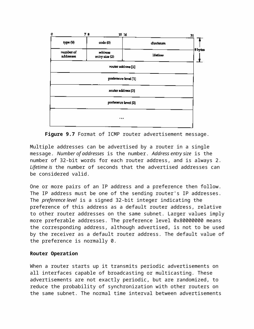
11 3.460626 (0.2389) vangogh.login > slip.1023: P 6:8(2) ack 5 12 3.489414 (0.0288) vangogh.login > slip.1023: P 8:10(2) ack 1 13 3.640356 (0.1509) slip.1023 > vangogh.login: . ack 10

Figure 19.7 Disabling the Nagle algorithm during an Rlogin session.

It is instructive and more enlightening to take this output and construct the time line, knowing that some of the segments are crossing in the network. Also, this example requires careful examination of the sequence numbers, to follow the data flow. We show this in Figure 19.8. We have numbered the segments to correspond with the numbering in the tcpdump output in Figure 19.7.

The first change we notice is that all 3 bytes are sent when they're ready (segments 1,2, and 3). "There is no delay-the Nagle algorithm has been disabled.

The next packet we see in the tcpdump output (segment 4) contains byte 5 from the server with an ACK 4. This is wrong. The client immediately responds with an ACK 2 (it is not delayed), not an ACK 6, since it wasn't expecting byte 5 to arrive. It appears a data segment was lost. We show this with a dashed line in Figure 19.8.

How do we know this lost segment contained bytes 2, 3, and 4, along with an ACK 3? The next byte we're expecting is byte number 2, as announced by segment 5. (Whenever TCP receives out-of-order data beyond the next expected sequence number, it normally responds with an acknowledgment specifying the sequence number of the next byte it expects to receive.) Also, since the missing segment contained bytes 2, 3, and 4, it means the server must have received segment 2, so the missing segment must have specified an ACK 3 (the sequence number of the next byte the server is expecting to receive.) Finally, notice that the retransmission, segment 6, contains data from the missing segment and segment 4. This is called repacketization, and we'll discuss it more in Section 21.11.

Returning to our discussion of disabling the Nagle algorithm, we can see the 3 bytes of the next special function key that we type is sent as three individual segments (8, 9, and 10). This time the server echoes the byte in segment 8 first (segment II), and then echoes the bytes in segments 9 and 10 (segment 12).

What we've seen in this example is that the default use of the Nagle algorithm can cause additional delays when multibyte keystrokes are entered while running an interactive application across a WAN. We return to the topic of timeout and retransmission in Chapter 21.

Figure 19.8 Time line for Figure 19.7 (Nagle algorithm disabled).

TCP Timeout and Retransmission

21.1 Introduction

TCP provides a reliable transport layer. One of the ways it provides reliability is for each end to acknowledge the data it receives from. the other end. But data segments and acknowledgments can get lost. TCP handles this by setting a timeout when it sends data, and if the data isn't acknowledged when the timeout expires, it retransmits the data. A

critical element of any implementation is the timeout and retransmission strategy. How is the timeout interval determined, and how frequently does a retransmission occur?

We've already seen two examples of timeout and retransmission: (1) In the ICMP port unreachable example in Section 6.5 we saw the TFTP client using UDP employing a simple (and poor) timeout and retransmission strategy: it assumed 5 seconds was an adequate timeout period and retransmitted every 5 seconds. (2) In the ARP example to a nonexistent host (Section 4.5), we saw that when TCP tried to establish the connection it retransmitted its SYN using a longer delay between each retransmission. TCP manages four different timers for each connection.

1. A retransmission timer is used when expecting an acknowledgment from the other end. This chapter looks at this timer in detail, along with related issues such as congestion avoidance.

2. A persist timer keeps window size information flowing even if the other end closes its receive window. Chapter 22 describes this timer.

3. A keepalive timer detects when the other end on an otherwise idle connection crashes or reboots. Chapter 23 describes this timer.

4. A 2MSL timer measures the time a connection has been in the TIME_WAIT state. We described this state in Section 18.6.

In this chapter we start with a simple example of TCP's timeout and retransmission and then move to a larger example that lets us look at all the details involved in TCP's timer management. We look at how typical implementations measure the round-trip time of TCP segments and how TCP uses these measurements to estimate the retransmission timeout of the next segment it transmits. We then look at TCP's congestion avoidance-what TCP does when packets are lost-and follow through an actual example where packets are lost. We also look at the newer fast retransmit and fast recovery algorithms, and see how they let TCP detect lost packets faster than waiting for a timer to expire.

21.2 Simple Timeout and Retransmission Example

Let's first look at the retransmission strategy used by TCP. We'll establish a connection, send some data to verify that everything is OK, disconnect the cable, send some more data, and watch what TCP does:

bsdi % telnet svr4 discard Trying 140.252.13.34...Connected to svr4.Escape character is '^]'.Hello, world send this line normally and hi disconnect cable before sending this line Connection closed by foreign host. output whenTCP gives up after 9 minutes

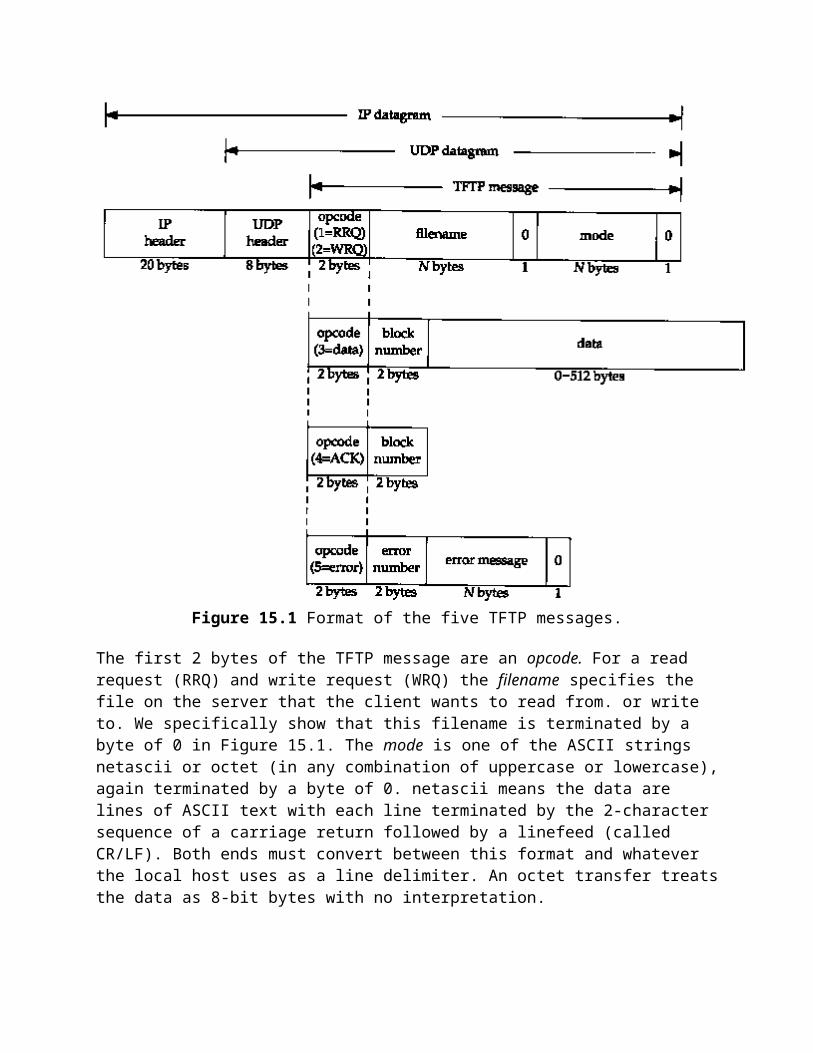
Figure 21.1 shows the tcpdump output. (We have removed all the type-of-service information that is set by bsdi.)

1 0.0 bsdi.1029 > svr4.discard: S 1747921409:1747921409(0) win 4096 <mss 1024>

2 0.004811 ( 0.0048) svr4.discard > bsdi.1029: S 3416685569:3416685569(0) ack 1747921410 win 4096 <mss 1024>

3 0.006441 ( 0.0016) bsdi.1029 > svr4.discard: . ack 1 win 4096 4 6.102290 ( 6.0958) bsdi.1029 > svr4.discard: P 1:15(14) ack 1 win 4096 5 6.259410 ( 0.1571) svr4.discard > bsdi.1029: . ack 15 win 4096 6 24.480158 (18.2207) bsdi.1029 > svr4.discard: P 15:23(8) ack 1 win 4096 7 25.493733 ( 1.0136) bsdi.1029 > svr4.discard: P 15:23(8) ack 1 win 4096 8 28.493795 ( 3.0001) bsdi.1029 > svr4.discard: P 15:23(8) ack 1 win 4096 9 34.493971 ( 6.0002) bsdi.1029 > svr4.discard: P 15:23(8) ack 1 win 4096 10 46.484427 (11.9905) bsdi.1029 > svr4.discard: P 15:23(8) ack 1 win 4096 11 70.485105 (24.0007) bsdi.1029 > svr4.discard: P 15:23(8) ack 1 win 4096 12 118.486408 (48.0013) bsdi.1029 > svr4.discard: P 15:23(8) ack 1 win 4096 13 182.488164 (64.0018) bsdi.1029 > svr4.discard: P 15:23(8) ack 1 win 4096 14 246.489921 (64.0018) bsdi.1029 > svr4.discard: P 15:23(8) ack 1 win 4096 15 310.491678 (64.0018) bsdi.1029 > svr4.discard: P 15:23(8) ack 1 win 4096 16 374.493431 (64.0018) bsdi.1029 > svr4.discard: P 15:23(8) ack 1 win 4096 17 438.495196 (64.0018) bsdi.1029 > svr4.discard: P 15:23(8) ack 1 win 4096 18 502.486941 (63.9917) bsdi.1029 > svr4.discard: P 15:23(8) ack 1 win 4096 19 566.488478 (64.0015) bsdi.1029 > svr4.discard: R 23:23(0) ack 1 win 4096

Figure 21.1 Simple example of TCP's timeout and retransmission.

Lines 1, 2, and 3 correspond to the normal TCP connection establishment. Line 4 is the transmission of "hello, world" (12 characters plus the carriage return and linefeed), and line 5 is its acknowledgment. We then disconnect the Ethernet cable from svr4.

Line 6 shows "and hi" being sent. Lines 7-18 are 12 retransmissions of that segment, and line 19 is when the sending TCP finally gives up and sends a reset.

Examine the time difference between successive retransmissions: with rounding they occur 1, 3, 6, 12, 24, 48, and then 64 seconds apart. We'll see later in this chapter that the first timeout is actually set for 1.5 seconds after the first transmission. (The reason it occurs 1.0136 seconds after the first transmission, and not exactly 1.5 seconds, was explained in Figure 18.7.) After this the timeout value is doubled for each retransmission, with an upper limit of 64 seconds.

This doubling is called an exponential backoff. Compare this to the TFTP example in Section 6.5, where every retransmission occurred 5 seconds after the previous.

The time difference between the first transmission of the packet (line 6 at time 24.480) and the reset (line 19 at time 566.488) is about 9 minutes. Modem TCP's are persistent when trying to send data!

On most implementations this total timeout value is not tunable. Solaris 2.2 allows the administrator to change this (the tcp_ip_abort_interval variable in Section E.4) and its default is only 2 minutes, not the more common 9 minutes.

21.3 Round-Trip Time Measurement

Fundamental to TCP's timeout and retransmission is the measurement of the round-trip time (RTT) experienced on a given connection. We expect this can change over time, as routes might change and as network traffic changes, and TCP should track these changes and modify its timeout accordingly.

First TCP must measure the RTT between sending a byte with a particular sequence number and receiving an acknowledgment that covers that sequence number. Recall from the previous chapter that normally there is not a one-to-one correspondence between data segments and ACKs. In Figure 20.1 this means that one RTT that can be measured by the sender is the time between the transmission of segment 4 (data bytes 1-1024) and the reception of segment 7 (the ACK of bytes 1-2048), even though this ACK is for an additional 1024 bytes. We'll use M to denote the measured RTT.

The original TCP specification had TCP update a smoothed RTT estimator (called R) using the low-pass filter

R <- R + (1-)M

where is a smoothing factor with a recommended value of 0.9. This smoothed RTT is updated every time a new measurement is made. Ninety percent of each new estimate is from the previous estimate and 10% is from the new measurement.

Given this smoothed estimator, which changes as the RTT changes, RFC 793 recommended the retransmission timeout value (RTO) be set to

RTO = R

where is a delay variance factor with a recommended value of 2.

[Jacobson 1988] details the problems with this approach, basically that it can't keep up with wide fluctuations in the RTT, causing unnecessary retransmissions. As Jacobson notes, unnecessary retransmissions add to the network load, when the network is already loaded. It is the network equivalent of pouring gasoline on a fire.

What's needed is to keep track of the variance in the RTT measurements, in addition to the smoothed RTT estimator. Calculating the RTO based on both the mean and variance

provides much better response to wide fluctuations in the round-trip times, than just calculating the RTO as a constant multiple of the mean. Figures 5 and 6 in [Jacobson 1988] show a comparison of the RFC 793 RTO values for some actual round-trip times, versus the RTO calculations we show below, which take into account the variance of the round-trip times.

As described by Jacobson, the mean deviation is a good approximation to the standard deviation, but easier to compute. (Calculating the standard deviation requires a square root.) This leads to the following equations that are applied to each RTT measurement M.

Err = M - AA <- A + gErr

D <- D+ h(|Err| - D)RTO = A + 4D

where A is the smoothed RTT (an estimator of the average) and D is the smoothed mean deviation. Err is the difference between the measured value just obtained and the current RTT estimator. Both A and D are used to calculate the next retransmission timeout (RTO). The gain g is for the average and is set to 1/8 (0.125). The gain for the deviation is h and is set to 0.25. The larger gain for the deviation makes the RTO go up faster when the RTT changes.

[Jacobson 1988] specified 2D in the calculation of RTO, but after further research, [Jacobson 1990c] changed the value to 4D, which is what appeared in the BSD Net/1 implementation.

Jacobson specifies a way to do all these calculations using integer arithmetic, and this is the implementation typically used. (That's one reason g, h, and the multiplier 4 are all powers of 2, so the operations can be done using shifts instead of multiplies and divides.)

Comparing the original method with Jacobson's, we see that the calculations of the smoothed average are similar ( is one minus the gain g) but a different gain is used. Also, Jacobson's calculation of the RTO depends on both the smoothed RTT and the smoothed mean deviation, whereas the original method used a multiple of the smoothed RTT.

We'll see how these estimators are initialized in the next section, when we go through an example.

Karn's Algorithm

A problem occurs when a packet is retransmitted. Say a packet is transmitted, a timeout occurs, the RTO is backed off as shown in Section 21.2, the packet is retransmitted with the longer RTO, and an acknowledgment is received. Is the ACK for the first transmission or the second? This is called the retransmission ambiguity problem.

[Karn and Partridge 1987] specify that when a timeout and retransmission occur, we cannot update the RTT estimators when the acknowledgment for the retransmitted data finally arrives. This is because we don't know to which transmission the ACK corresponds. (Perhaps the first transmission was delayed and not thrown away, or perhaps the ACK of the first transmission was delayed.)

Also, since the data was retransmitted, and the exponential backoff has been applied to the RTO, we reuse this backed off RTO for the next transmission. Don't calculate a new RTO until an acknowledgment is received for a segment that was not retransmitted.

21.4 An RTT Example

We'll use the following example throughout this chapter to examine various implementation details of TCP's timeout and retransmission, slow start, and congestion avoidance.

Using our sock program, 32768 bytes of data are sent from our host slip to the discard service on the host vangogh.cs.berkeley.edu using the command:

slip % sock -D -i -n32 vangogh.cs.berkeley.edu discard

From the figure on the inside front cover, slip is connected from the 140.252.1 Ethernet by two SLIP links, and from there across the Internet to the destination. With two 9600 bits/sec SLIP links, we expect some measurable delays.

This command performs 32 1024-byte writes, and since the MTU between slip and bsdi is 296, this becomes 128 segments, each with 256 bytes of user data. The total time for the transfer is about 45 seconds and we see one timeout and three retransmissions.

While this transfer was running we ran tcpdump on the host slip and captured all the segments sent and received. Additionally we specified the -D option to turn on socket debugging (Section A.6). We were then able to run a modified version of the trpt(8) program to print numerous variables in the connection control block relating to the round-trip timing, slow start, and congestion avoidance.

Given the volume of trace output, we can't show it all. Instead we'll look at pieces as we proceed through the chapter. Figure 21.2 shows the transfer of data and acknowledgments for the first 5 seconds. We have modified this output slightly from our previous display of tcpdump output. Although we only measure the times that the packet is sent or received on the host running tcpdump, in this figure we want to show that the packets are crossing in the network (which they are, since this LAN connection is not like a shared Ethernet), and show when the receiving host is probably generating the ACKs. (We have also removed all the window advertisements from this figure, slip always advertised a window of 4096, and vangogh always advertised a window of 8192.)

Figure 21.2 Packet exchange and RTT measurement.

Also note in this figure that we have numbered the segments 1-13 and 15, in the order in which they were sent or received on the host slip. This correlates with the tcpdump output that was collected on this host.

Round-Trip Time Measurements

Three curly braces have been placed on the left side of the time line indicating which segments were timed for RTT calculations. Not all data segments are timed.

Most Berkeley-derived implementations of TCP measure only one RTT value per connection at any time. If the timer for a given connection is already in use when a data segment is transmitted, that segment is not timed.

The timing is done by incrementing a counter every time the 500-ms TCP timer routine is invoked. This means that a segment whose acknowledgment arrives 550 rns after the segment was sent could end up with either a 1 tick RTT (implying 500 ms) or a 2 tick RTT (implying 1000 ms).

In addition to this tick counter for each connection, the starting sequence number of the data in the segment is also remembered. When an acknowledgment that includes this sequence number is received, the timer is turned off. If the data was not retransmitted when the ACK arrives, the smoothed RTT and smoothed mean deviation are updated based on this new measurement.

The timer for the connection in Figure 21.2 is started when segment 1 is transmitted, and turned off when its acknowledgment (segment 2) arrives. Although its RTT is 1.061 seconds (from the tcpdump output), examining the socket debug information shows that three of TCP's clock ticks occurred during this period, implying an RTT of 1500 ms.

The next segment timed is number 3. When segment 4 is transmitted 2.4 ms later, it cannot be timed, since the timer for this connection is already in use. When segment 5 arrives, acknowledging the data that was being timed, its RTT is calculated to be 1 tick (500 ms), even though we see that its RTT is 0.808 seconds from the tcpdump output.

The timer is started again when segment 6 is transmitted, and turned off when its acknowledgment (segment 10) is received 1.015 seconds later. The measured RTT is 2 clock ticks. Segments 7 and 9 cannot be timed, since the timer is already being used. Also, when segment 8 is received (the ACK of 769), nothing is updated since the acknowledgment was not for bytes being timed.

Figure 21.3 shows the relationship in this example between the actual RTTs that we can determine from the tcpdump output, and the counted clock ticks.

Figure 21.3 RTT measurements and clock ticks.

On the top we show the clock ticks, every 500 ms. On the bottom we show the times output by tcpdump, and when the timer for the connection is turned on and off. We know that 3 ticks occur between sending segment 1 and receiving segment 2, 1.061 seconds later, so we

assume the first tick occurs at time 0.03. (The first tick must be between 0.00 and 0.061.) The figure then shows how the second measured RTT was counted as 1 tick, and the third as 2 ticks.

In this complete example, 128 segments were transmitted, and 18 RTT samples were collected. Figure 21.4 shows the measured RTT (taken from the tcpdump output) along with the RTO used by TCP for the timeout (taken from the socket debug output). The x-axis starts at time 0 in Figure 21.2, when the first data segment is transmitted, not when the first SYN is transmitted.

Figure 21.4 Measured RTT and TCP's calculated RTO for example.

The first three data points for the measured RTT correspond to the 3 RTTs that we show in Figure 21.2. The gaps in the RTT samples around times 10, 14, and 21 are caused by retransmissions that took place there (which we'll show later in this chapter). Kam's algorithm prevents us from updating our estimators until another segment is transmitted and acknowledged. Also note that for this implementation, TCP's calculated RTO is always a multiple of 500 ms.

RTT Estimator Calculations

Let's see how the RTT estimators (the smoothed RTT and the smoothed mean deviation) are initialized and updated, and how each retransmission timeout is calculated.

The variables A and D are initialized to 0 and 3 seconds, respectively. The initial retransmission timeout is calculated using the formula

RTO = A + 2D = 0 + 2x3 = 6 seconds

(The factor 2D is used only for this initial calculation. After this 4D is added to A to calculate RTO, as shown earlier.) This is the RTO for the transmission of the initial SYN.

It turns out that this initial SYN is lost, and we time out and retransmit. Figure 21.5 shows the first four lines from the tcpdump output file.

1 0.0 slip.1024 > vangogh. discard: S 35648001:35648001(0) win 4096 <mss 256>

2 5.802377 (5.8024) slip.1024 > vangogh.discard: S 35648001:35648001(0) win 4096 <mss 256>

3 6.269395 (0.4670) vangogh.discard > slip.1024: S 1365512705:1365512705(0) ack 35648002 win 8192 <mss 512>

4 6.270796 (0.0014) slip. 1024 > vangogh.discard: . ack 1 win 4096 Figure 21.5 Timeout and retransmission of initial SYN.

When the timeout occurs after 5.802 seconds, the current RTO is calculated as

RTO = A + 4D = 0 + 4x3 = 12 seconds

The exponential backoff is then applied to the RTO of 12. Since this is the first timeout we use a multiplier of 2, giving the next timeout value as 24 seconds. The next timeout is calculated using a multiplier of 4, giving a value of 48 seconds: 12 x 4. (These initial RTOs for the first SYN on a connection, 6 seconds and then 24 seconds, are what we saw in Figure 4.5.)

The ACK arrives 467 ms after the retransmission. The values of A and D are not updated, because of Karn's algorithm dealing with the retransmission ambiguity. The next segment sent is the ACK on line 4, but it is not timed since it is only an ACK. (Only segments containing data are timed.)

When the first data segment is sent (segment 1 in Figure 21.2) the RTO is not changed, again owing to Karn's algorithm. The current value of 24 seconds is reused until an RTT measurement is made. This means the RTO for time 0 in Figure 21.4 is really 24, but we didn't plot that point.

When the ACK for the first data segment arrives (segment 2 in Figure 21.2), three clock ticks were counted and our estimators are initialized as

A = M + 0.5 = 1.5 + 0.5 = 2D = A/2 = 1

(The value 1.5 for M is for 3 clock ticks.) The previous initialization of A and D to 0 and 3 was for the initial RTO calculation. This initialization is for the first calculation of the estimators using the first RTT measurement M. The RTO is calculated as

RTO = A + 4D = 2 + 4x1 = 6 seconds

When the ACK for the second data segment arrives (segment 5 in Figure 21.2), 1 clock tick is counted (0.5 seconds) and our estimators are updated as

Err = M - A = 0.5 - 2 = -1.5A = A + gErr = 2 - 0.125x1.5 = 1.8125

D = D + h(|Err| - D) = 1 + 0.25x(1.5 - 1) = 1.125RTO = A + 4D = 1.8125 + 4x1.125 = 6.3125

There are some subtleties in the fixed-point representations of Err, A, and D, and the fixed-point calculations that are actually used (which we've shown in floating-point for simplicity). These differences yield an RTO of 6 seconds (not 6.3125), which is what we plot in Figure 21.4 for time 1.871.

Slow Start

We described the slow start algorithm in Section 20.6. We can see it in action again in Figure 21.2.

Only one segment is initially transmitted on the connection, and its acknowledgment must be received before another segment is transmitted. When segment 2 is received, two more segments are transmitted.

21.5 Congestion Example

Now let's look at the transmission of the data segments. Figure 21.6 is a plot of the starting sequence number in a segment versus the time that the segment was sent. This provides a nice way to visualize the data transmission. Normally the data points should move up and to the right, with the slope of the points being the transfer rate. Retransmissions will appear as motion down and to the right.

At the beginning of Section 21.4 we said the total time for the transfer was about 45 seconds, but we show only 35 seconds in this figure. These 35 seconds account for sending the data segments only. The first data segment was not transmitted until 6.3 seconds after the first SYN was sent, because the first SYN appears to have been lost and was retransmitted (Figure 21.5). Also, after the final data segment and the FIN were sent (at time 34.1 in Figure 21.6) it took another 4.0 seconds to receive the final 14 ACKs from the receiver, before the receiver's FIN was received.

Figure 21.6 Sending of 32768 bytes of data from slip to vangogh.

We can immediately see the three retransmissions around times 10, 14, and 21 in Figure 21.6. At each of these three points we can also see that only one segment is retransmitted, because only one dot dips below the upward slope.

Let's examine the first of these dips in detail (around the 10-second mark). From the tcpdump output we can put together Figure 21.7.

Figure 21.7 Packet exchange for retransmission around the 10-second mark.

We have removed all the window advertisements from this figure, except for segment 72, which we discuss below, slip always advertised a window of 4096, and vangogh advertised a window of 8192. The segments are numbered in this figure as a continuation of Figure 21.2, where the first data segment across the connection was numbered 1. As in Figure 21.2, the segments are numbered according to their send or receive order on the host slip, where tcpdump was being run. We have also removed a few segments that have no relevance to the discussion (44, 47, and 49, all ACKs from vangogh).

It appears that segment 45 got lost or arrived damaged-we can't tell from this output. What we see on the host slip is the acknowledgment for everything up through but not including byte 6657 (segment 58), followed by eight more ACKs of this same sequence number. It is the reception of segment 62, the third of the duplicate ACKs, that forces the retransmission of the data starting at sequence number 6657 (segment 63). Indeed, Berkeley-derived implementations count the number of duplicate ACKs received, and when the third one is received, assume that a segment has been lost and retransmit only one segment, starting with that sequence number. This is Jacobson's fast retransmit algorithm, which is followed by his fast recovery algorithm. We discuss both algorithms in Section 21.7.

Notice that after the retransmission (segment 63), the sender continues normal data transmission (segments 67, 69, and 71). TCP does not wait for the other end to acknowledge the retransmission.

Let's examine what happens at the receiver. When normal data is received in sequence (segment 43), the receiving TCP passes the 256 bytes of data to the user process. But the next segment received (segment 46) is out of order: the starting sequence number of the data (6913) is not the next expected sequence number (6657). TCP saves the 256 bytes of data and responds with an ACK of the highest sequence number successfully received, plus one (6657). The next seven segments received by vangogh (48, 50, 52, 54, 55, 57, and 59) are also out of order. The data is saved by the receiving TCP, and duplicate ACKs are generated.

Currently there is no way for TCP to tell the other end that a segment is missing. Also, TCP cannot acknowledge out-of-order data. All vangogh can do at this point is continue sending the ACKs of 6657.

When the missing data arrives (segment 63), the receiving TCP now has data bytes 6657-8960 in its buffer, and passes these 2304 bytes to the user process. All 2304 bytes are acknowledged in segment 72. Also notice that this ACK advertises a window of 5888 (8192 - 2304), since the user process hasn't had a chance to read the 2304 bytes that are ready for it.

If we look in detail at the tcpdump output for the dips around times 14 and 21 in Figure 21.6, we see that they too were caused by the receipt of three duplicate ACKs, indicating that a packet had been lost. In each of these cases only a single packet was retransmitted.

We'll continue this example in Section 21.8, after describing more about the congestion avoidance algorithms.

21.6 Congestion Avoidance Algorithm

Slow start, which we described in Section 20.6, is the way to initiate data flow across a connection. But at some point we'll reach the limit of an intervening router, and packets can be dropped. Congestion avoidance is a way to deal with lost packets. It is described in [Jacobson 1988].

The assumption of the algorithm is that packet loss caused by damage is very small (much less than 1%), therefore the loss of a packet signals congestion somewhere in the network between the source and destination. There are two indications of packet loss: a timeout occurring and the receipt of duplicate ACKs. (We saw the latter in Section 21.5. If we are using a timeout as an indication of congestion, we can see the need for a good RTT algorithm, such as that described in Section 21.3.)

Congestion avoidance and slow start are independent algorithms with different objectives. But when congestion occurs we want to slow down the transmission rate of packets into the network, and then invoke slow start to get things going again. In practice they are implemented together.

Congestion avoidance and slow start require that two variables be maintained for each connection: a congestion window, cwnd, and a slow start threshold size, ssthresh. The combined algorithm operates as follows:

1. Initialization for a given connection sets cwnd to one segment and ssthresh to 65535 bytes.

2. The TCP output routine never sends more than the minimum of cwnd and the receiver's advertised window.

Congestion avoidance is flow control imposed by the sender, while the advertised window is flow control imposed by the receiver. The former is based on the sender's assessment of perceived network congestion; the latter is related to the amount of available buffer space at the receiver for this connection.

3. When congestion occurs (indicated by a timeout or the reception of duplicate ACKs), one-half of the current window size (the minimum of cwnd and the receiver's advertised window, but at least two segments) is saved in ssthresh. Additionally, if the congestion is indicated by a timeout, cwnd is set to one segment (i.e., slow start).

4. When new data is acknowledged by the other end, we increase cwnd, but the way it increases depends on whether we're performing slow start or congestion avoidance.

If cwnd is less than or equal to ssthresh, we're doing slow start; otherwise we're doing congestion avoidance. Slow start continues until we're halfway to where we were when congestion occurred (since we recorded half of the window size that got us into trouble in step 2), and then congestion avoidance takes over.

Slow start has cwnd start at one segment, and be incremented by one segment every time an ACK is received. As mentioned in Section 20.6, this opens the window exponentially: send one segment, then two, then four, and so on.

Congestion avoidance dictates that cwnd be incremented by 1/cwnd each time an ACK is received. This is an additive increase, compared to slow start's exponential increase. We want to increase cwnd by at most one segment each round-trip time

(regardless how many ACKs are received in that RTT), whereas slow start will increment cwnd by the number of ACKs received in a round-trip time.

All 4.3BSD releases and 4.4BSD incorrectly add a small fraction of the segment size (the segment size divided by 8) during congestion avoidance. This is wrong and should not be emulated in future releases [Floyd 1994]. Nevertheless, we show this term in future calculations, to arrive at the same answer as the (incorrect) implementation.

The 4.3BSD Tahoe release, described in [Leffler et al. 1989], performed slow start only if the other end was on a different network. This was changed with the 4.3BSD Reno release so that slow start is always performed.

Figure 21.8 is a visual description of slow start and congestion avoidance. We show cwnd and ssthresh in units of segments, but they're really maintained in bytes.

Figure 21.8 Visualization of slow start and congestion avoidance.

In this figure we assume that congestion occurred when cwnd had a value of 32 segments. ssthresh is then set to 16 segments and cwnd is set to 1 segment. One segment is then sent at time 0 and assuming its ACK is returned at time 1, cwnd is incremented to 2 segments. Two segments are then sent and assuming their ACKs return by time 2, cwnd is incremented to 4 segments (once for each ACK). This exponential increase continues until cwnd equals ssthresh, after 8 ACKs are received between times 3 and 4. From this point on the increase in cwnd is linear, with a maximum increase of one segment per round-trip time.

As we can see in this figure, the term "slow start" is not completely correct. It is a slower transmission of packets than what caused the congestion, but the rate of increase in the number of packets injected into the network increases during slow start. The rate of increase doesn't slow down until ssthresh is reached, when congestion avoidance takes over.

21.7 Fast Retransmit and Fast Recovery Algorithms

Modifications to the congestion avoidance algorithm were proposed in 1990 [Jacobson 1990b]. We've already seen these modifications in action in our congestion example (Section 21.5).

Before describing the change, realize that TCP is required to generate an immediate acknowledgment (a duplicate ACK) when an out-of-order segment is received. This duplicate ACK should not be delayed. The purpose of this duplicate ACK is to let the other end know that a segment was received out of order, and to tell it what sequence number is expected.

Since we don't know whether a duplicate ACK is caused by a lost segment or just a reordering of segments, we wait for a small number of duplicate ACKs to be received. It is assumed that if there is just a reordering of the segments, there will be only one or two duplicate ACKs before the reordered segment is processed, which will then generate a new ACK. If three or more duplicate ACKs are received in a row, it is a strong indication that a segment has been lost. (We saw this in Section 21.5.) We then perform a retransmission of what appears to be the missing segment, without waiting for a retransmission timer to expire. This is the fast retransmit algorithm. Next, congestion avoidance, but not slow start is performed. This is the fast recovery algorithm.

In Figure 21.7 we saw that slow start was not performed after the three duplicate ACKs were received. Instead the sender did the retransmission, followed by three more segments with new data (segments 67, 69, and 71), before the acknowledgment of the retransmission was received (segment 72).

The reason for not performing slow start in this case is that the receipt of the duplicate ACKs tells us more than just a packet has been lost. Since the receiver can only generate the duplicate ACK when another segment is received, that segment has left the network and is in the receiver's buffer. That is, there is still data flowing between the two ends, and we don't want to reduce the flow abruptly by going into slow start. This algorithms are usually implemented together as follows.

1. When the third duplicate ACK is received, set ssthresh to one-half the current congestion window, cwnd.

Retransmit the missing segment. Set cwnd to ssthresh plus 3 times the segment size.

2. Each time another duplicate ACK arrives, increment cwnd by the segment size and transmit a packet (if allowed by the new value of cwnd).

3. When the next ACK arrives that acknowledges new data, set cwnd to ssthresh (the value set in step 1). This should be the ACK of the retransmission from step 1, one round-trip time after the retransmission. Additionally, this ACK should acknowledge all the intermediate segments sent between the lost packet and the receipt of the

first duplicate ACK. This step is congestion avoidance, since we're slowing down to one-half the rate we were at when the packet was lost.

We'll see what happens to the two variables cwnd and ssthresh in the calculations in the next section.

The fast retransmit algorithm first appeared in the 4.3BSD Tahoe release, but it was incorrectly followed by slow start. The fast recovery algorithm appeared in the 4.3BSD Reno release.

21.8 Congestion Example (Continued)

Watching a connection using tcpdump and the socket debug option (which we described in Section 21.4) we can see the values of cwnd and ssthresh as each segment is transmitted. If the MSS is 256 bytes, the initial values of cwnd and ssthresh are 256 and 65535, respectively. Each time an ACK is received we can see cwnd incremented by the MSS, taking on the values 512, 768, 1024, 1280, and so on. Assuming congestion doesn't occur, eventually the congestion window will exceed the receiver's advertised window, meaning the advertised window will limit the data flow.

A more interesting example is to see what happens when congestion occurs. We'll use the same example from Section 21.4. There were four occurrences of congestion while this example was being run. There was a timeout on the transmission of the initial SYN to establish the connection (Figure 21.5), followed by three lost packets during the data transfer (Figure 21.6).

Figure 21.9 shows the values of the two variables cwnd and ssthresh when the initial SYN is retransmitted, followed by the first seven data segments. (We showed the exchange of the initial data segments and their ACKs in Figure 21.2.) We show the data bytes transmitted using the tcpdump notation: 1:257(256) means bytes 1 through 256.

Segment# Action Variable

(Figure 21.2) Send Receive Comment cwnd ssthresh

SYN

SYN

ACK

SYN, ACK

-

initialize

timeoutretransmit

-

256

256

-

65535

512

-

1234

1:257(256)

257:513(256)513:769(256)

ACK 257 slow start 512 512

56789

101112

769:1025(256)1025:1281(256)

1281:1537(256)

1537:1793(256)-

ACK 513

ACK 769

ACK 1025

ACK 1281

slow start

cong. avoid

cong. avoid

cong. avoid

768

885

991

1089

512

512

512

512

Figure 21.9 Example of congestion avoidance.

When the timeout of the SYN occurs, ssthresh is set to its minimum value (512 bytes. which is two segments for this example), cwnd is set to one segment (256 bytes, which it was already at) to enter the slow start phase.

When the SYN and ACK are received, nothing happens to the two variables, since new data is not being acknowledged.

When the ACK 257 arrives, we are still in slow start since cwnd is less than or equal to ssthresh, so cwnd in incremented by 256. The same thing happens when the ACK 512 arrives.

When the ACK 769 arrives we are no longer in slow start, but enter congestior avoidance. The new value for cwnd is calculated as

cwnd <- cwnd + segsize x segsize/cwnd + segsize/8

This is the 1/cwnd increase that we mentioned earlier, taking into account that cwnd is really maintained in bytes and not segments. For this example we calculate

cwnd <- 768 + 256 x 256 / 768 + 256 / 8

which equals 885 (using integer arithmetic). When the next ACK 1025 arrives we calculate

cwnd <- 885 + 256x256/885 + 256/8

which equals 991. (In these expressions we include the incorrect 256/8 term to match the values calculated by the implementation, as we noted in Section 21.6)

This additive increase in cwnd continues until the first retransmission, around the 10-second mark in Figure 21.6. Figure 21.10 is a plot of the same data as in Figure 21.6, with the value of cwnd added.

Figure 21.10 Value of cwnd and send sequence number while data is being transmitted.

The first six values for cwnd in this figure are the values we calculated for Figure 21.9. It is impossible in this figure to tell the difference visually between the exponential increase during slow start and the additive increase during congestion avoidance, because the slow start phase is so quick.

We need to explain what is happening at the three points where a retransmission occurs. Recall that each of the retransmissions took place because three duplicate ACKs were received, indicating a packet had been lost. This is the fast retransmit algorithm from Section 21.7. ssthresh is immediately set to one-half the window size that was in effect when the retransmission took place, but cwnd is allowed to keep increasing while the duplicate ACKs are received, since each duplicate ACK means that a segment has left the network (the receiving TCP has buffered it, waiting for the missing hole in the data to arrive). This is the fast recovery algorithm.

Figure 21.11 is similar to Figure 21.9, showing the values of cwnd and ssthresh. The segment numbers in the first column correspond to Figure 21.7.

Segment# Action Variable

(Figure 21.7) Send Receive Comment cwnd ssthresh

58 596061

8705:8961(256)ACK 6657

ACK 6657ACK 6657

ACK of new data

duplicate ACK #1duplicate ACK #2

2426

24262426

512

512512

6263646566676869707172

6657:6913(256)

8961:9217(256)

9217:9473(256)

9473:9729(256).

ACK 6657

ACK 6657ACK 6657ACK 6657

ACK 6657

ACK 6657

ACK 8961

duplicate ACK #3retransmission

duplicate ACK #4duplicate ACK #5duplicate ACK #6

duplicate ACK #7

duplicate ACK #8

ACK of new data

1792

204823042560

2816

3072

1280

1024

102410241024

1024

1024

1024

Figure 21.11 Example of congestion avoidance (continued).

The values for cwnd have been increasing continually, from the final value in Figure 21.9 for segment 12 (1089), to the first value in Figure 21.11 for segment 58 (2426). The value of ssthresh has remained the same (512), since there have been no retransmissions in this period.

When the first two duplicate ACKs arrive (segments 60 and 61) they are counted, and cwnd is left alone. (This is the flat portion of Figure 21.10 preceding the retransmission.) When the third one arrives, however, ssthresh is set to one-half cwnd (rounded down to the next multiple of the segment size), cwnd is set to ssthresh plus the number of duplicate ACKs times the segment size (i.e., 1024 plus 3 times 256). The retransmission is then sent.

Five more duplicate ACKs arrive (segments 64-66, 68, and 70) and cwnd is incremented by the segment size each time. Finally a new ACK arrives (segment 72) and cwnd is set to ssthresh (1024) and the normal congestion avoidance takes over. Since cwnd is less than or equal to ssthresh (they are equal), the segment size is added to cwnd, giving a value of 1280. When the next new ACK is received (which isn't shown in Figure 21.11), cwnd is greater than ssthresh, so cwnd is set to 1363.

During the fast retransmit and fast recovery phase, we transmit new data after receiving the duplicate ACKs in segments 66, 68, and 70, but not after receiving the duplicate ACKs in segments 64 and 65. The reason is the value of cwnd, versus the number of unacknowledged bytes of data. When segment 64 is received, cwnd equals 2048, but we have 2304 unacknowledged bytes (nine segments: 46, 48, 50, 52, 54, 55, 57, 59, and 63). We can't send anything. When segment 65 arrives, cwnd equals 2304, so we still can't send anything. But when segment 66 arrives, cwnd equals 2560, so we can send a new data segment. Similarly when segment 68 arrives, cwnd equals 2816, which is greater than the 2560 bytes of unacknowledged data, so we can send another new data segment. The same scenario happens when segment 70 is received.

W^hen the next retransmission takes place at time 14.3 in Figure 21.10, it is also triggered by the reception of three duplicate ACKs, so we see the same increase in cwnd as one more duplicate ACK arrives, followed by a decrease to 1024.

The retransmission at time 21.1 in Figure 21.10 is also triggered by duplicate ACKs. We receive three more duplicates after the retransmission, so we see three additional increases in cwnd, followed by a decrease to 1280. For the remainder of the transfer cwnd increases linearly to a final value of 3615.

Per-Route Metrics

Newer TCP implementations maintain many of the metrics that we've described in this chapter in the routing table entry. When a TCP connection is closed, if enough data was sent to obtain meaningful statistics, and if the routing table entry for the destination is not a default route, the following information is saved in the routing table entry, for the next use of the entry: the smoothed RTT, the smoothed mean deviation, and the slow start threshold. The quantity "enough data" is 16 windows of data. This gives 16 RTT samples, which allows the smoothed RTT filter to converge within 5% of the correct value.

Additionally, the route(8) command can be used by the administrator to set the metrics for a given route: the three values mentioned in the preceding paragraph, along with the MTU, the outbound bandwidth-delay product (Section 20.7), and the inbound bandwidth-delay product.

When a new TCP connection is established, either actively or passively, if the routing table entry being used for the connection has values for these metrics, the corresponding variable is initialized from the metrics.

UNIT-V

SNMP: Simple Network Management Protocol

25.1 Introduction

As the number of networks within an organization grows, along with the diversity of systems comprising this internet (routers from various vendors, hosts with embedded router functionality, terminal servers, etc.), managing all these systems within a coherent framework becomes important. This chapter looks at the standards used within the Internet protocol suite for network management.

Network management of a TCP/IP internet consists of network management stations (managers) communicating with network elements. The network elements can be anything that runs the TCP/IP protocol suite: hosts, routers, X terminals, terminal servers, printers, and so on. The software in the network element that runs the management software is called the agent. Management stations are normally workstations with color monitors that graphically display relevant facts about the elements being monitored (which links are up and down, volume of traffic across various links over time, etc.).

"The communication can be two way: the manager asking the agent for a specific value ("how many ICMP port unreachables have you generated?"), or the agent telling the manager that something important happened ("an attached interface has gone down"). Also, the manager should be able to set variables in the agent ("change the value of the default IP TTL to 64"), in addition to reading variables from the agent. TCP/IP network management consists of three pieces.

1. A Management Information Base (MIB) that specifies what variables the network elements maintain (the information that can be queried and set by the manager). RFC 1213 [McCloghrie and Rose 1991] defines the second version of this, called MIB-II.

2. A set of common structures and an identification scheme used to reference the variables in the MIB. This is called the Structure of Management Information (SMI) and is specified in RFC 1155 [Rose and McCloghrie 1990]. For example, the SMI specifies that a Counter is a nonnegative integer that counts from 0 through 4,294,967,295 and then wraps around to 0.

3. The protocol between the manager and the element, called the Simple Network Management Protocol (SNMP). RFC 1157 [Case et al. 1990] specifies the protocol. This details the format of the packets exchanged. Although a wide variety of transport protocols could be used, UDP is normally used with SNMP.

These RFCs define what is now called SNMPv1, or just SNMP, which is the topic of this chapter. During 1993 additional RFCs were published specifying SNMP Version 2 (SNMPv2), which we describe in Section 25.12.

Our approach to SNMP in this chapter is to describe the protocol between the manager and the agent first, and then look at the data types for the variables maintained by the agent. We describe the database of information maintained by the agent (the MIB), looking at the groups that we've described in this text: IP, UDP, TCP, and so on. We show examples at each point along the way, tying network management back to the protocol concepts from earlier chapters.

25.2 Protocol

SNMP defines only five types of messages that are exchanged between the manager and agent.

1. Fetch the value of one or more variables: the get-request operator. 2. Fetch the next variable after one or more specified variables: the get-next-request

operator. (We describe what we mean by "next" later in this chapter.)

3. Set the value of one or more variables: the set-request operator.

4. Return the value of one or more variables: the get-response operator. This is the message returned by the agent to the manager in response to the get-request, get-next-request, and set-request operators.

5. Notify the manager when something happens on the agent: the trap operator.

The first three messages are sent from the manager to the agent, and the last two are from the agent to the manager. (We'll refer to the first three as the get, get-next, and set operators.) Figure 25.1 summarizes these five operators.

Since four of the five SNMP messages are simple request-reply protocols (the manager sends a request, the agent sends back a reply) SNMP uses UDP. This means that a request from the manager may not arrive at the agent, and the agent's reply may not make it back to the manager. The manager probably wants to implement a timeout and retransmission.

Figure 25.1 Summary of the five SNMP operators.

The manager sends its three requests to UDP port 161. The agent sends traps to UDP port 162. By using two different port numbers, a single system can easily run both a manager and an agent. (See Exercise 25.1.)

Figure 25.2 shows the format of the five SNMP messages, encapsulated in a UDP datagram.

Figure 25.2 Format of the five SNMP messages.

In this figure we specify the size in bytes of the IP and UDP headers only. This is because the encoding used for the SNMP message-called ASN.1 and BER, which we describe later in this chapter-varies depending on the type of variable and its value.

The version is 0. This value is really the version number minus one, as the version of SNMP that we describe is called SNMPv1.

Figure 25.3 shows the values for the PDU type. (PDU stands for Protocol Data Unit, a fancy word for "packet.")

PDU type Name

0 get-request

1 get-next-request

2 set-request

3 get-response

4 trap

Figure 25.3 PDU types for SNMP messages.

The community is a character string that is a cleartext password between the manager and agent. A common value is the 6-character string public.

For the get, get-next, and set operators, the request ID is set by the manager, and returned by the agent in the get-response message. We've seen this type of variable with other UDP applications. (Recall the DNS identification field in Figure 14.3, and the transaction ID field in Figure 16.2.) It lets the client (the manager in this case) match the responses from the server (the agent) to the queries that the client issued. "This field also allows the manager to issue multiple requests to one or more agents, and then be able to sort out the returned replies.

The error status is an integer returned by the agent specifying an error. Figure 25.4 shows the values, names, and descriptions.

error status

Name Description

0 noError all is OK

1 tooBig agent could not fit reply into a single SNMP message

2 noSuchName operation specified a nonexistent variable

3 badValue a set operation specified an invalid value or syntax

4 readonly manager tried to modify a read-only variable

5 genErr some other error

Figure 25.4 SNMP error status values.

If an error occurred, the error index is an integer offset specifying which variable was in error. It is set by the agent only for the noSuchName, badValue, and readonly errors.

A list of variable names and values follows in the get, get-next, and set requests. The value portion is ignored for the get and get-next operators.

For the trap operator (a PDU type of 4), the format of the SNMP message changes. We describe the fields in the trap header when we describe this operator in Section 25.10.

25.3 Structure of Management Information

SNMP uses only a few different types of data. In this section we'll look at those data types, without worrying about how the data is actually encoded (that is, the bit pattern used to store the data).

INTEGER. Some variables are declared as an integer with no restrictions (e.g., the MTU of an interface), some are defined as taking on specific values (e.g., the IP forwarding flag is 1 if forwarding is enabled or 2 if forwarding is disabled), and others are defined with a minimum and maximum value (e.g., UDP and TCP port numbers are between 0 and 65535).

OCTET STRING. A string of 0 or more 8-bit bytes. Each byte has a value between 0 and 255. In the BER encoding used for this data type and the next, a count of the number of bytes in the string precedes the string. These strings are not null-terminated strings.

DisplayString. A string of 0 or more 8-bit bytes, but each byte must be a character from the NVT ASCII set (Section 26.4). All variables of this type in the MIB-II must contain no more than 255 characters. (A O-length string is OK.)

OBJECT IDENTIFIER. We describe these in the next section.

NULL. This indicates that the corresponding variable has no value. It is used, for example, as the value of all the variables in a get or get-next request, since the values are being queried, not set.

lpAddress. An OCTET STRING of length 4, with 1 byte for each byte of the IP address.

PhysAddress. An OCTET STRING specifying a physical address (e.g., a 6-byte Ethernet address).

Counter. A nonnegative integer whose value increases monotonically from 0 to 232-1 (4,294,967,295), and then wraps back to 0.

Gauge. A nonnegative integer between 0 and 232 -1, whose value can increase or decrease, but latches at its maximum value. That is, if the value increments to 232 - 1, it stays there until reset. The MIB variable tcpCurrEstab is an example: it is the number of TCP connections currently in the ESTABLISHED or CLOSE_WAIT state.

TimeTicks. A counter that counts the time in hundredths of a second since some epoch. Different variables can specify this counter from a different epoch, so the epoch used for each variable of this type is specified when the variable is declared in the MIB. For example, the variable sysUpTime is the number of hundredths of a second that the agent has been up.

SEQUENCE. This is similar to a structure in the C programming language. For example, we'll see that the MIB defines a SEQUENCE named UdpEntry containing information about an agent's active UDP end points. (By "active" we mean ports currently in use by an application.) Two entries are in the structure:

1. udpLocalAddress, of type lpAddress, containing the local IP address.

2. udpLocalPort, of type INTEGER, in the range 0 through 65535, specifying the local port number.

SEQUENCE OF. This is the definition of a vector, with all elements having the same data type. If each element has a simple data type, such as an integer, then we have a simple vector (a one-dimensional array). But we'll see that SNMP uses this data type with each element of the vector being a SEQUENCE (structure). We can then think of it as a two-dimensional array or table.

For example, the UDP listener table is named udpTable and it is a SEQUENCE OF the 2-element SEQUENCE (structure) UdpEntry that we just described. Figure 25.5 shows this two-dimensional array.

Figure 25.5 UDP listener table (udpTable) as a two-dimensional array in SNMP.

The number of rows in these tables is not specified by SNMP, but we'll see that a manager using the get-next operator (Section 25.7) can determine when the final row of a table has been returned. Also, in Section 25.6 we'll see how the manager specifies which row of a table it wants to get or set.

25.4 Object Identifiers

An object identifier is a data type specifying an authoritatively named object. By "authoritative" we mean that these identifiers are not assigned randomly, but are allocated by some organization that has responsibility for a group of identifiers.

An object identifier is a sequence of integers separated by decimal points. These integers traverse a tree structure, similar to the DNS (Figure 14.1) or a Unix filesystem. There is an unnamed root at the top of the tree where the object identifiers start. (This is the same direction of tree traversal that's used with a Unix filesystem.)

Figure 25.6 shows the structure of this tree when used with SNMP. All variables in the MIB start with the object identifier 1.3.6.1.2.1.

Each node in the tree is also given a textual name. The name corresponding to the object identifier 1.3.6.1.2.1 is iso.org.dod.internet.mgmt.mib. These names are for human readability. The names of the MIB variables that are in the packets exchanged between the manager and agent (Figure 25.2) are the numeric object identifiers, all of which begin with 1.3.6.1.2.1.

Figure 25.6 Object identifiers in the Management Information Base.

Besides the mib object identifiers in Figure 25.6 we also show one named iso.org.dod.internet.private.enterprises (1.3.6.1.4.1). "This is where vendor-specific MIBs are located. The Assigned Numbers RFC lists around 400 identifiers registered below this node.

25.5 Introduction to the Management Information Base

The Management Information Base, or MIB, is the database of information maintained by the agent that the manager can query or set. We describe what's called MIB-II, specified in RFC 1213 [McCloghrie and Rose 1991].

As shown in Figure 25.6, the MIB is divided into groups named system, interfaces, at (address translation), ip, and so on.

In this section we describe only the variables in the UDP group. This is a simple group with only a few variables and a single table. In the next sections we use this group to show the details of instance identification, lexicographic ordering, and some simple examples of these features. After these examples we return to the MIB in Section 25.8 and describe some of the other groups in the MIB.

In Figure 25.6 we showed the group named udp beneath mib. Figure 25.7 shows the structure of the UDP group.

Figure 25.7 Tree structure of IP address table.

There are four simple variables and a table containing two simple variables. Figure 25.8 describes the four simple variables.

Name Datatype R/W Description

udpInDatagrams Counter Number of UDP datagrams delivered to user processes.

udpNoPorts Counter Number of received UDP datagrams for which no application process was at the destination port.

udpInErrors Counter Number of undeliverable UDP datagrams for reasons other than no application at destination port (e.g., UDP checksum error).

udpOutDatagrams Counter Number of UDP datagrams sent.

Figure 25.8 Simple variables in udp group.

We'll use this format to describe all the MIB variables in this chapter. The column labeled "R/W" is empty if the variable is read-only, or contains a bullet (*) if the variable is read-

write. We always include this column, even if all the variables in a group are read-only (since they are in the udp group) to reiterate that none of the variables can be set by the manager. Also, when the data type is an INTEGER with bounds, we specify the lower limit and upper limit, as we do for the UDP port number in the next figure.

Figure 25.9 describes the two simple variables in the udpTable.

UDP listener table, index = < udpLocalAddress >.< udpLocalPort >

Name Datatype R/W Description

udpLocalAddress lpAddress Local IP address for this listener. 0.0.0.0 indicates the listener is willing to receive datagrams on any interface.

udpLocalPort [0..65535] Local port number for this listener.

Figure 25.9 Variables in udpTable.

Each time we describe the variables in an SNMP table, the first row of the figure indicates the value of the "index" used to reference each row of the table. We show some examples of this in the next section.

Case Diagrams

There is a relationship between the first three counters in Figure 25.8. Case Diagrams [Case and Partridge 1989] visually illustrate the relationships between the various MIB variables in a given group. Figure 25.10 is a Case Diagram for the UDP group.

Figure 25.10 Case Diagram for UDP group.

What this diagram shows is that the number of UDP datagrams delivered to applications (udpInDatagrams) is the number of UDP datagrams delivered from IP to UDP, minus udpInErrors, minus udpNoPorts. Also, the number of UDP datagrams delivered to IP (udpOutDatagrams) is the number passed to UDP from the applications. This illustrates that udpInDatagrams does not include udpInErrors or udpNoPorts.

These diagrams were used during the development of the MIB to verify that all data paths for a packet were accounted for. [Rose 1994] shows Case Diagrams for all the groups in the MIB.

25.6 Instance Identification

Every variable in the MIB must be identified when SNMP is referencing it, to fetch or set its value. First, only leaf nodes are referenced. SNMP does not manipulate entire rows or columns of tables. Returning to Figure 25.7, the leaf nodes are the four that we described in Figure 25.8 and the two in Figure 25.9. mib, udp, udpTabie, and udpEntry are not leaf nodes.

Simple Variables

Simple variables are referenced by appending ".0" to the variable's object identifier. For example, the counter udpInDatagrams from Figure 25.8, whose object identifier is 1.3.6.1.2.1.7.1, is referenced as 1.3.6.1.2.1.7.1.0. The textual name of this reference is iso.org.dod.internet.mgmt.mib.udp.udpInDatagrams.0.

Although references to this variable are normally abbreviated as just udpInDatagrams.0, we reiterate that the name of the variable that appears in the SNMP message (Figure 25.2) is the object identifier 1.3.6.1.2.1.7.1.0.

Tables

Instance identification of table entries is more detailed. Let's return to the UDP listener table (Figure 25.7).

One or more indexes are specified in the MIB for each table. For the UDP listener table, the MIB defines the index as the combination of the two variables udpLocalAddress, which is an IP address, and udpLocalPort, which is an integer. (We showed this index in the top row in Figure 25.9.)

Assume there are three rows in the UDP listener table: the first row is for IP address 0.0.0.0 and port 67, the second for 0.0.0.0 and port 161, and the third for 0.0.0.0 and port 520. Figure 25.11 shows this table.

udpLocalAddress udpLocalPort

0.0.0.0 67

0.0.0.0 161

0.0.0.0 520

Figure 25.11 Sample UDP listener table.

This implies that the system is willing to receive UDP datagrams on any interface for ports 67 (BOOTP server), 161 (SNMP), and 520 (RIP). The three rows in the table are referenced as shown in Figure 25.12.

Lexicographic Ordering

There is an implied ordering in the MIB based on the order of the object identifiers. All the entries in MIB tables are lexicographically ordered by their object identifiers. This means the six variables in Figure 25.12 are ordered in the MIB as shown in Figure 25.13. Two key points result from this lexicographic ordering.

Row Object identifier Abbreviated name Value

11.3.6.1.2.1.7.5.1.1.0.0.0.0.671.3.6.1.2.1.7.5.1.2.0.0.0.0.67

udpLocalAddress.0.0.0.0.67udpLocalPort.0.0.0.0.67

0.0.0.067

21.3.6.1.2.1.7.5.1.1.0.0.0.0.1611.3.6.1.2.1.7.5.1.2.0.0.0.0.161

udpLocalAddress.0.0.0.0.161udpLocalPort.0.0.0.0.161

0.0.0.0 161

31.3.6.1.2.1.7.5.1.1.0.0.0.0.5201.3.6.1.2.1.7.5.1.2.0.0.0.0.520

udpLocalAddress.0.0.0.0.520udpLocalPort.0.0.0.0.520

0.0.0.0 520

Figure 25.12 Instance identification for rows in UDP listener table.

ColumnObject identifier

(lexicographically ordered)Abbreviated name Value

11.3.6.1.2.1.7.5.1.1.0.0.0.0.67 1.3.6.1.2.1.7.5.1.1.0.0.0.0.1611.3.6.1.2.1.7.5.1.1.0.0.0.0.520

udpLocalAddress.0.0.0.0.67udpLocalAddress.0.0.0.0.161udpLocalAddress.0.0.0.0.520

0.0.0.00.0.0.00.0.0.0

21.3.6.1.2.1.7.5.1.2.0.0.0.0.67 1.3.6.1.2.1.7.5.1.2.0.0.0.0.1611.3.6.1.2.1.7.5.1.2.0.0.0.0.520

udpLocalPort.0.0.0.0.67udpLocalPort.0.0.0.0.161udpLocalPort.0.0.0.0.520

67161520

Figure 25.13 Lexicographic ordering of UDP listener table.1. Since all instances for a given variable (udpLocalAddress) appear before all

instances for the next variable in the table (udpLocalPort), this implies that tables are accessed in a column-row order. This results from the lexicographic ordering of the object identifiers, not the human-readable names.

2. The ordering of the rows in a table depends on the values of the indexes for the table. In Figure 25.13, 67 is lexicographically less than 161, which is lexicographically less than 520.

Figure 25.14 shows this column-row order for our sample UDP listener table.

Figure 25.14 UDP listener table, showing column-row ordering.

We'll also see this column-row ordering when we use the get-next operator in the next section.

25.7 Simple Examples

In this section we'll show some examples that fetch the values of variables from an SNMP agent. The software used to query the agent is called snmpi and is from the ISODE system. Both are described briefly in [Rose 1994].

Simple Variables

We'll query a router for two simple variables from the UDP group:

sun % snmpi -a gateway -c secret

snmpi> get udpInDatagrams.0 udpNoPorta.0udplnDatagrams.0=616168udpNoPorts.0=33

snmpi> quit

The -a option identifies the agent we want to communicate with, and the -c option specifies the SNMP community. It is a password supplied by the client (snmpi in this case) and if the server (the agent in the system gateway) recognizes the community name, it honors the manager's request. An agent could allow clients within one community read-only access to its variables, and clients in another community read-write access.

The program outputs its snmpi> prompt, and we can type commands such as get, which translates into an SNMP get-request message. When we're done, we type quit. (In all further examples we'll remove this final quit command.) Figure 25.15 shows the two lines of tcpdump output for this example.

1 0.0 sun.1024 > gateway.161: GetRequest(42) 1.3.6.1.2.1.7.1.0 1.3.6.1.2.1.7.2.0

2 0.348875 (0.3489) gateway.161 > sun.1024: GetResponse(46)1.3.6.1.2.1.7.1.0=6161681.3.6.1.2.1.7.2.0=33

Figure 25.15 tcpdump output for simple SNMP query.

The request for the two variables is sent in a single UDP datagram, and the response is also a single UDP datagram.

We show the variables as their respective object identifiers, because that is what's sent in the SNMP messages. We had to specify the instance of the two variables as 0. Notice also that the name of the variable (its object identifier) is always returned in the response. We'll see below that this is required for the get-next operator to work.

get-next Operator

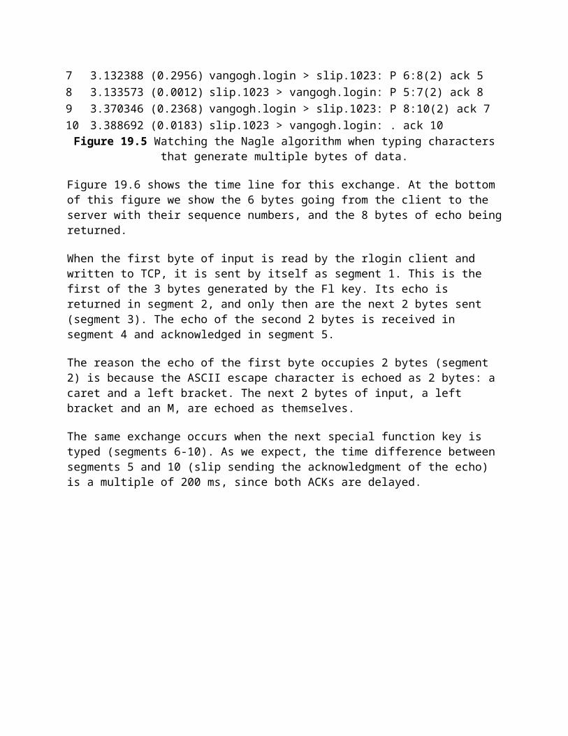
The operation of the get-next operator is based on the lexicographic ordering of the MIB. We start the following example by asking for the next object identifier after udp (without specifying any instance, since this is not a leaf object). This returns the first object in the UDP group. We then ask for the next entry after this one, and the second entry is returned. We repeat this one more time to get the third entry:

sun % sninpi -a gateway -c secret

snmpi> next udpudpInDatagrams.0=616318

snmpi> next udpInDatagraros.0 udpNoPorts.0=33

snmpi> next udpNoPorts.0 udpInErrors.0=0

This example shows why a get-next operator must return the name of the variable: we ask the agent for the next variable, and the agent returns its name and value.

Using the get-next operator in this fashion, one could imagine a manager with a loop that starts at the beginning of the MIB and queries the agent for every variable that the agent maintains. Another use of this operator is to iterate through tables.

Table Access

We can reiterate the column-row ordering of tables using our simple query program to step through the entire UDP listener table. We start by asking for the next variable after udpTable. Since this is not a leaf object we can't specify an instance, but the get-next operator still returns the next object in the table. We then work our way through the table, with the agent returning the next variable, in column-row order:

sun % snmpi-a gateway -c secret

snmpi> next udpTable udpLocalAddress.0.0.0.0.67=0.0.0.0

snmpi> next udpLocalAddress.0.0.0.0.67 udpLocalAddress.0.0.0.0.161-0.0.0.0

snmpi> next udpLocalAddress.0.0.0.0.161 udpLocalAddress.0.0.0.0.52 0=0.0.0.0

snmpi> next udpLocalAddress.0.0.0.0.520 udpLocalPort.0.0.0.0.67=67

snmpi> next udpLocalPort.0.0.0.0.67 udpLocalPort.0.0.0.0.161=161

snmpi> next udpLocalPort.0.0.0.0.161 udpLocalPort.0.0.0.0.520=520

snmpi> next udpLocalPort.0.0.0.0.520 snmpInPkts.0=59 we're finished with the UDP listener table

We see that the order returned corresponds to Figure 25.14.

How does a manager know when it reaches the end of a table? Since the response to the get-next operator contains the name of the next entry in the MIB after the table, the manager can tell when the name changes. In our example the last entry in the UDP listener table is followed by the variable snmpInPkts.

Telnet and Rlogin: Remote Login

26.1 Introduction

Remote login is one of the most popular Internet applications. Instead of having a hardwired terminal on each host, we can login to one host and then remote login across the network to any other host (that we have an account on, of course).

Two popular applications provide remote login across TCP/IP internets.

1. Telnet is a standard application that almost every TCP/IP implementation provides. It works between hosts that use different operating systems. Telnet uses option negotiation between the client and server to determine what features each end can provide.

2. Rlogin is from Berkeley Unix and was developed to work between Unix systems only, but it has been ported to other operating systems also.

In this chapter we look at both Telnet and Rlogin. We start with Rlogin because it's simpler.

Telnet is one of the oldest of the Internet applications, dating back to 1969 on the ARPANET. Its name is actually an acronym that stands for "telecommunications network protocol."

Remote login uses the client-server paradigm. Figure 26.1 shows the typical arrangement of the Telnet client and server. (We could draw a similar picture for an Rlogin client and server.)

Figure 26.1 Overview of Telnet client-server.

There are numerous points in this figure.

1. The Telnet client interacts with both the user at the terminal and the TCP/IP protocols. Normally everything we type is sent across the TCP connection, and everything received from the connection is output to our terminal.

2. The Telnet server often deals with what's called a pseudo-terminal device, at least under Unix systems. This makes it appear to the login shell that's invoked on the server, and to any programs run by the login shell, that they're talking to a terminal device. Some applications, such as full-screen editors, assume they're talking to a terminal device. Indeed, making the login shell on the server think that it's talking to a terminal is often one of the hardest programming aspects involved in writing a remote login server.

3. Only a single TCP connection is used. Since there are times when the Telnet client must talk to the Telnet server (and vice versa) there needs to be some way to delineate commands that are sent across the connection, versus user data. We'll see how both Telnet and Rlogin handle this.

4. We show dashed boxes in Figure 26.1 to note that the terminal and pseudoterminal drivers, along with the TCP/IP implementation, are normally part of the operating system kernel. The Telnet client and server, however, are often user applications.

5. We show the login shell on the server host to reiterate that we have to login to the server. We must have an account on that system to login to it, using either Telnet or Rlogin.

It is interesting to compare the complexity of Telnet and Rlogin by looking at the number of lines of source code required to implement the client and server for each. Figure 26.2 shows these counts for the standard Telnet and Rlogin client and server, as distributed in different versions from Berkeley (Figure 1.10).

Figure 26.2 Comparison of Telnet/Rlogin/client/server, number of lines of source code.

It is the continuing addition of new options to Telnet that causes its implementation to grow, while Rlogin remains simple and stable.

Remote login is not a high-volume data transfer application. As we've mentioned earlier, lots of small packets are normally exchanged between the two end systems. [Paxson 1993] found that the ratio of bytes sent by the client (the user typing at the terminal) to the number of bytes sent back by the server is about 1:20. This is because we type short commands that often generate lots of output.

26.2 Rlogin Protocol

Rlogin appeared with 4.2BSD and was intended for remote login only between Unix hosts. This makes it a simpler protocol than Telnet, since option negotiation is not required when the operating system on the client and server are known in advance. Over the past few years, Rlogin has also been ported to several non-Unix environments.

RFC 1282 [Kantor 1991] specifies the Rlogin protocol. As with the Routing Information Protocol (RIP) RFC, however, this one was written after Rlogin had been in use for many years. Chapter 15 of [Stevens 1990] describes programming remote login clients and servers, and provides the complete source code for the Rlogin client and server. Chapters 25 and 26 of [Comer and Stevens 1993] provide the implementation details and source code for a Telnet client.

Application Startup

Rlogin uses a single TCP connection between the client and server. After the normal TCP connection establishment is complete, the following application protocol takes place between the client and server.

1. The client writes four strings to the server; (a) a byte of 0, (b) the login name of the user on the client host, terminated by a byte of 0, (c) the login name of the user on

the server host, terminated by a byte of 0, (d) the name of the user's terminal type, followed by a slash, followed by the terminal speed, terminated by a byte of 0. Two login names are required because users aren't required to have the same login name on each system.

The terminal type is passed from the client to the server because many full-screen applications need to know it. The terminal speed is passed because some applications operate differently depending on the speed. For example, the vi editor works with a smaller window when operating at slower speeds, so it doesn't take forever to redraw the window.

2. The server responds with a byte of 0. 3. The server has the option of asking the user to enter a password. This is handled as

normal data exchange across the Rlogin connection-there is no special protocol. The server sends a string to the client (which the client displays on the terminal), often Password:. If the client does not enter a password within some time limit (often 60 seconds), the server closes the connection.

We can create a file in our home directory on the server (named .rhosts) with lines containing a hostname and our username. If we login from the specified host with that username, we are not prompted for a password. Most security texts, such as [Curry 1992], strongly suggest never using this feature because of the security hole it presents.

If we are prompted by the server for a password, what we type is sent to the server as cleartext. Each character of the password that we type is sent as is. Anyone who can read the raw network packets can read the characters of our password. Newer implementations of the Rlogin client, such as 4.4BSD, first try to use Kerberos, which avoids sending cleartext passwords across the network. This requires a compatible server that also supports Kerberos. ([Curry 1992] describes Kerberos in more detail.)

4. The server normally sends a request to the client asking for the terminal's window size (described later).

The client sends 1 byte at a time to the server and all echoing is done by the server. We saw this in Section 19.2. Also, the Nagle algorithm is normally enabled (Section 19.4), causing multiple input bytes to be sent as a single TCP segment across slower networks. The operation is simple: everything typed by the user is sent to the server, and everything sent by the server to the client is displayed on the terminal.

Additional commands exist that can be sent from the client to the server and from the server to the client. Let's first describe the scenarios that require these commands.

Flow Control

By default, flow control is done by the Rlogin client. The client recognizes the ASCII STOP and START characters (Control-S and Control-Q) typed by the user, and stops or starts the terminal output.

If this isn't done, each time we type Control-S to stop the terminal output, the Control-S character is sent across the network to the server, and the server stops writing to the network-but up to a window's worth of output may have been already written by the server and will be displayed before the output is stopped. Hundreds or thousands of bytes of data will scroll down the screen before the output stops. Figure 26.3 shows this scenario.

Figure 26.3 Rlogin connection if server performs STOP/START processing.

To an interactive user this delayed response to the Control-S character is bad.

Sometimes, however, the application running on the server needs to interpret each byte of input, and doesn't want the client looking at the input bytes and treating Control-S and Control-Q specially. (The emacs editor is an example of an application that uses these two characters for its own commands.) To handle this, the capability is provided for the server to tell the client whether or not to perform flow control.

Client Interrupt

A problem similar to flow control occurs when we type the interrupt key (often DELETE or Control-C), to abort the process currently running on the server. The scenario is similar to what we show in Figure 26.3, with up to one window full of data in the pipe from the server to the client, while the interrupt key makes its way across the connection in the other direction. We want the interrupt key to terminate what's being displayed on the screen as quickly as possible.

In both this case and the flow control scenario, it is rare for the flow of data from the client to the server to be stopped by flow control. This direction contains only characters that we type. Therefore it is not necessary for these special input characters (Control-S or interrupt) to be sent from the client to the server using TCP's urgent mode.

Window Size Changes

With a windowed display we can dynamically change the size of the window while an application is running. Some applications (typically those that manipulate the entire window, such as a full-screen editor) need to know these changes. Most current Unix systems provide the capability for an application to be told of these window size changes.

With remote login, however, the change in the window size occurs on the client, but the application that needs to be told is running on the server. Some form of notification is

required for the Rlogin client to tell the server that the window size has changed, and what the new size is.

Server to Client Commands

We can now summarize the four commands that the Rlogin server can send to the client across the TCP connection. The problem is that only a single TCP connection is used, so the server needs to mark these command bytes so the client knows to interpret them as commands, and not display the bytes on the terminal. TCP's urgent mode is used for this (Section 20.8).

When the server sends a command to the client, the server enters urgent mode with the last byte of urgent data being the command byte from the server. When the client receives the urgent mode notification, it reads from the connection, saving the data until the command byte (the last byte of urgent data) is encountered. The data that's saved by the client can be displayed on the terminal, or discarded, depending on the command. Figure 26.4 describes the four command bytes.

Byte Description

0x02

Flush output. The client discards all the data received from the server, up through the command byte (the last byte of urgent data). The client also discards any pending terminal output that may be buffered. The server sends this command when it receives the interrupt key from the client.

0x10 The client stops performing flow control.

0x20 The client resumes flow control processing.

0x80The client responds immediately by sending the current window size to the server, and notifies the server in the future if the window size changes. This command is normally sent by the server immediately after the connection is established.

Figure 26.4 Rlogin commands from the server to the client.

One reason for sending these commands using TCP's urgent mode is that the first command ("flush output") needs to be sent to the client even if the flow of data from the server to the client is stopped by TCP's windowed flow control. This condition-the server's output to the client being flow control stopped-is likely to occur, since processes running on the server can usually generate output faster than the client's terminal can display it. Conversely, it is rare for the flow of data from the client to the server to be flow control stopped, since this direction of data flow contains the characters that we type.

Recall our example in Figure 20.14 where we saw the urgent notification go across the connection even though the window size was 0. (We'll see another example of this in the next section.) The remaining three commands aren't time critical, but they use the same technique for symplicity.

Client to Server Commands

Only one command from the client to the server is currently defined: sending the current window size to the server. Window size changes from the client are not sent to the server unless the client receives the command 0x80 (Figure 26.4) from the server.

Again, since a single TCP connection is used, the client must have some way of marking the commands that it sends across the connection, so that the server doesn't pass them to the application running on the server. The client does this by sending 2 bytes of 0xff followed by two special flag bytes.

For the window size command, the two flag bytes are each the ASCII character s. Following this are four 16-bit values (in network byte order): the number of rows (e.g., 25), the number of characters per column (e.g., 80), the number of pixels in the X direction, and the number of pixels in the Y direction. Often the final two 16-bit values are 0, because most applications invoked by the Rlogin server deal with the size of the screen in characters, not pixels.

This form of command that we've described from the client to the server is called in-band signaling since the command bytes are sent in the normal stream of data. The bytes used to denote these in-band commands, 0xff, are chosen because we are unlikely to type keys that generate these bytes. But the Rlogin method is not perfect. If we could generate two consecutive bytes of 0xff from our keyboard, followed by two ASCII s's, the next 8 bytes we type will be interpreted as window sizes.

The Rlogin commands from the server to the client, which we described in Figure 26.4, are termed out-of-band signaling since the technique used is called "out-of-band data" by most APIs. But recall our discussion of TCP's urgent mode in Section 20.8 where we said that urgent mode is not out-of-band data, and the command byte is sent in the normal stream of data, pointed to by the urgent pointer.

Since in-band signaling is used from the client to the server, the server must examine every byte that it receives from the client, looking for two consecutive bytes of 0xff. But with out-of-band signaling used from the server to the client, the client does not need to examine the data that it receives from the server, until the server enters urgent mode. Even in urgent mode, the client only needs to look at the byte pointed to by the urgent pointer. Since the ratio of bytes from the client to server, versus from the server to client, is about 1:20, it makes sense to use in-band signaling for the low-volume data flow (client to server) and out-of-band signaling for the higher volume data flow (server to client).

Client Escapes

Normally everything we type to the Rlogin client is sent to the server. Occasionally, however, we want to talk directly to the Rlogin client program itself, and not have what we type sent to the server. This is done by typing a tilde (~) as the first character of a line, followed by one of the following four characters:

1. A period terminates the client.

2. The end-of-file character (often Control-D) terminates the client.

3. The job control suspend character (often Control-Z) suspends the client.

4. The job-control delayed-suspend character (often Control-Y) suspends only the client input. Everything we type is now interpreted by whatever program we run on the client host, but anything sent to the Rlogin client by the Rlogin server is output to our terminal. This can be used when we start a long running job on the server and we want to know when it outputs something, but we want to continue running other programs on the client.

The last two commands are supported only if the client Unix system supports job control.

26.3 Rlogin Examples

We'll look at two examples: the first shows the client-server protocol at the start of an Rlogin session, and the second shows what happens when we type our interrupt key to abort a running process on the server that is generating lots of output. In Figure 19.2 we showed the normal flow of data across an Rlogin session.

Initial Client-Server Protocol

Figure 26.5 shows the time line for an Rlogin connection from the host bsdi to the server on svr4. (We have removed the normal TCP connection establishment, the window advertisements, and the type-of-service information.)

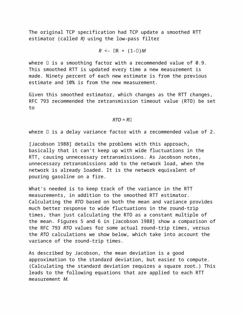
Figure 26.5 Time line for an Rlogin connection.

The protocol we described in the previous section can be seen in segments 1-9. The client sends a single byte of 0 (segment 1) followed by three strings (segment 3). In this example the three strings are rstevens (the login name on the client), rstevens (the login name on the server), and ibmpc3/9600 (the terminal type and speed). The server authenticates this and responds with a byte of 0 (segment 5).

The server then sends the window request command (segment 7). It is sent using TCP's urgent mode and again we see an implementation (SVR4) that uses the older, but more

common interpretation, where the urgent pointer specifies the sequence number plus one of the last byte of urgent data. The client responds with 12 bytes of data: 2 bytes of 0xff, 2 bytes of s, and 4 16-bit values.

The next four segments from the server (10, 12, 14, and 16) are the operating system greeting from the server. This is followed by the 7-byte shell prompt on the server: "svr4 % " in segment 18.

The data entered by the client is then sent 1 byte at a time, as shown in Figure 19.2. The connection can be closed by either end. If we type a command that causes the shell running on the server to terminate, the server's end does the active close. If we type an escape to the Rlogin client (normally a tilde), followed by a period or our end-of-file character, the client does the active close.

The client port number in Figure 26.5 is 1023, which is within the range controlled by the IANA (Section 1.9). The Rlogin protocol requires the client to have a port number less than 1024, termed a reserved port. On Unix systems, a client cannot obtain a reserved port unless the process has superuser privilege. This is part of the authentication between the client and server, which allows the user to login without entering a password. [Stevens 1990] discusses these reserved ports and the authentication used between the client and server in more detail.

Client Interrupt Key

Let's look at another example, this one involving TCP's urgent mode, when the flow of data has been stopped and we type the interrupt key. This example brings together many of the TCP algorithms we described earlier: urgent mode, silly window avoidance, windowed flow control, and the persist timer. We start the client on the host sun. We login to bsdi, output a big text file to the terminal, and then stop the output by typing Control-S. When the output stops we type our interrupt key (DELETE) to abort the program:

sun % rlogin bsdi all the operating system greetings

bsdi % cat /usr/share/misc/termcap output big file to terminal lots of terminal output we type Control-S to stop the output, and wait until the output stops

^? type our interrupt key, and this is echoed bsdi % then our prompt is output

The following points summarize the state of the client, the server, and the connection.

1. We stop the terminal output by typing Control-S. 2. The Rlogin client is blocked from writing to the terminal, since the terminal's output

buffer will fill.

3. The Rlogin client therefore cannot read from the network, so the client's TCP receive buffer fills.

4. The client's TCP advertises a window of 0 to stop the sender (the Rlogin server's TCP) when the receive buffer fills.

5. The server's TCP send buffer fills when its output is stopped by the client's window of 0.

6. The Rlogin server is stopped, since the send buffer is full. Therefore, the Rlogin server cannot read from the application that's running on the server (cat).

7. The cat application stops when its output buffer fills.

8. We then type the interrupt key to terminate the cat application on the server. This is sent from the client TCP to the server TCP because this direction of data flow has not been flow-control stopped.

9. The cat application receives the interrupt, and terminates. This causes its output buffer (which the Rlogin server is reading) to be flushed, which wakes up the Rlogin server. The Rlogin server then enters urgent mode and sends the "flush output" command (0x02) to the client.

Figure 26.6 is a summary of the data flow from the server to the client. (The sequence numbers are taken from the time line that we show next.)

Figure 26.6 Summary of data flow from server to client in Rlogin example.

The shaded portion of the send buffer is the unused portion of the 4096-byte buffer. Figure 26.7 is the time line for this example.

Figure 26.7 Rlogin example when client stops output and then aborts program on server.

In segments 1-3 the server sends full-sized segments to the client. The ACK in segment 4 only advertises a window of 1024 because the output is stopped: since the client can't write to the terminal, it can't read from the network. Segment 5 is not full sized, and the ACK in segment 6 advertises only the remaining space in the 4096-byte receive buffer. The client must advertise a window of 349 bytes, because if it advertised a window of 0 (which we might expect from silly window avoidance. Section 22.3), it would be moving the right edge of the window to the left, which must not happen (Section 20.3). Since the server can't send a full-sized buffer when it receives segment 6, it performs silly window avoidance, sends nothing, and sets a 5-second persist timer. When the timer expires it sends 349 bytes

(segment 7) and since the client's output is still stopped, the acknowledgment in segment 8 advertises a window of 0.

At this point we type our interrupt key and it is transmitted in segment 9. A window of 0 bytes is still advertised. When the Rlogin server receives the interrupt key it passes it to the application (cat) and the application terminates. Since the application was terminated by a terminal interrupt, its output is flushed and this is passed to the Rlogin server. This causes the server to send the "flush output" command to the client using TCP's urgent mode. We see this in segment 10. Notice, however, that the command byte of 0x02 is at sequence number 30146 (the urgent pointer minus one). There are 3419 bytes ahead of the command byte (sequence numbers 26727:30145) buffered at the server that the server wants to send.

Segment 10, with the urgent notification, contains the next byte of data from the server to the client (sequence number 26727). It does not contain the "flush output" command byte. The server can send this single byte in segment 10 because we saw in Section 22.2 that a sender with data can always probe a closed window by sending 1 byte of data. The client's TCP responds immediately in segment II with a zero window, but the receipt of the urgent notification in segment 10 causes the client's TCP to notify the Rlogin client that the other end of the connection has entered urgent mode.

Once the Rlogin client receives the urgent notification from its TCP, and starts reading the data that's already waiting for it, the window opens up (segment 13). The data buffered by the server is then sent (segments 14, 15, 17, and 18). The last of these contains the final byte of urgent data (sequence number 30146), which contains the command byte from the server to the client. When the client reads this byte it discards all the data that it read in segments 14, 15, 17, and 18, and flushes its terminal output queue. The next 2 bytes, in segment 19, are the echo of the interrupt key: "^?". The final segment we show (21) contains the shell prompt from the client.

This example shows how data can be buffered at both ends of the connection when the client types the interrupt key. If this action only discarded the 3419 bytes buffered at the server, without discarding the 4096 bytes at the client, these 4096 bytes of data, along with whatever was buffered in the terminal output queue on the client, would be output.

26.4 Telnet Protocol

Telnet was designed to work between any host (i.e., any operating system) and any terminal. Its specification in RFC 854 [Postel and Reynolds 1983a] defines the lowest common denominator terminal, called the network virtual terminal (NVT). The NVT is an imaginary device from which both ends of the connection, the client and server, map their real terminal to and from. That is, the client operating system must map whatever type of terminal the user is on to the NVT. The server must then map the NVT into whatever terminal type the server supports.

The NVT is a character device with a keyboard and printer. Data typed by the user on the keyboard is sent to the server, and data received from the server is output to the printer. By default the client echoes what the user types to the printer, but we'll see that options are normally supported to change this.

NVT ASCII

The term NVT ASCII refers to the 7-bit U.S. variant of the ASCII character set used throughout the Internet protocol suite. Each 7-bit character is sent as an 8-bit byte, with the high-order bit set to 0.

An end-of-line is transmitted as the 2-character sequence CR (carriage return) followed by an LF (linefeed). We show this as \r\n. A carriage return is transmitted as the 2-character sequence CR followed by a NUL (byte of 0). We show this as \r\0.

In the following chapters we'll see that FTP, SMTP, Finger, and Whois all use NVT ASCII for client commands and server responses.

Telnet Commands

Telnet uses in-band signaling in both directions. The byte 0xff (255 decimal) is called IAC, for "interpret as command." The next byte is the command byte. To send the data byte 255, two consecutive bytes of 255 are sent. (In the previous paragraph we said that the data stream is NVT ASCII, which are 7-bit values, implying a data byte of 255 cannot be sent by Telnet. There is a binary option for Telnet, RFC 856 [Postel and Reynolds 1983b], which we don't discuss, that allows 8-bit data transmission.) Figure 26.8 lists all the Telnet commands.

NameCode

(decimal)Description

EOF 236 end-of-file

SUSP 237 suspend current process (job control)

ABORT 238 abort process

EOR 239 end of record

SE 240 suboption end

NOP 241 no operation

DM 242 data mark

BRK 243 break

IP 244 interrupt process

AO 245 abort output

AYT 246 are you there?

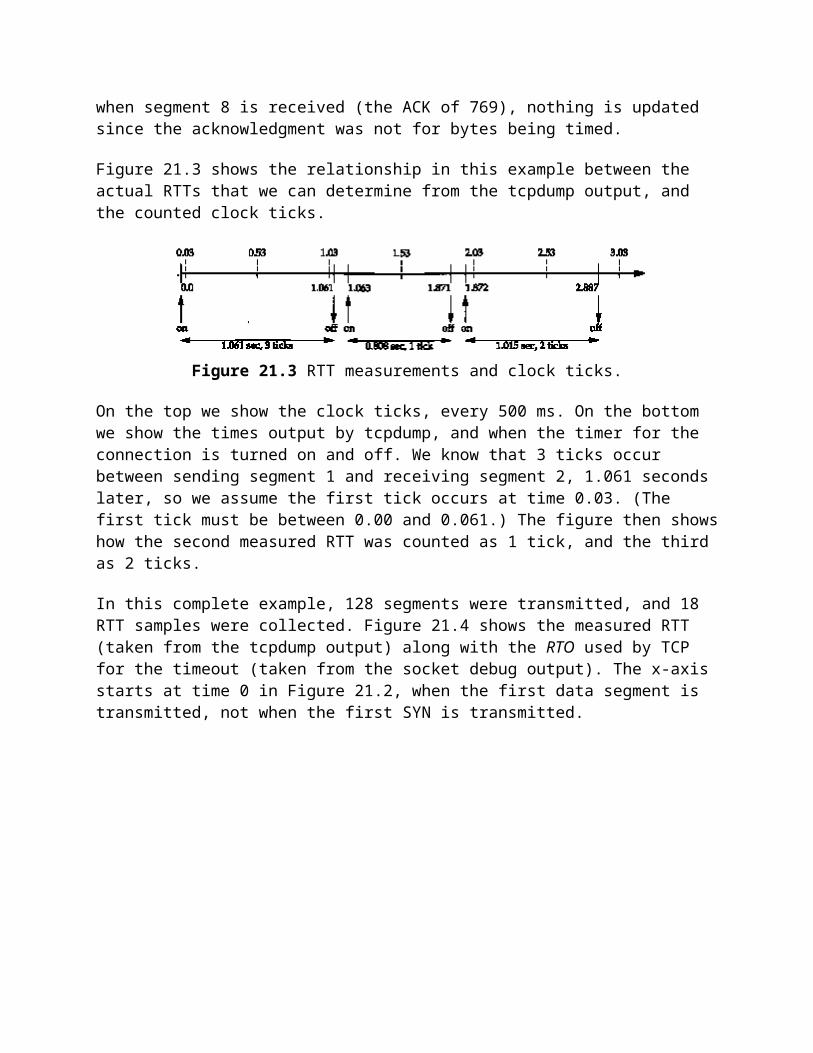
EC 247 escape character

EL 248 erase line

GA 249 go ahead

SB 250 suboption begin

WILL 251 option negotiation (Figure 26.9)

WONT 252 option negotiation

IX) 253 option negotiation

DONT 254 option negotiation

IAC 255 data byte 255

Figure 26.8 Telnet commands, when preceded by IAC (255).

Since many of these commands are rarely used, we describe the important commands when we encounter them in the discussion below and in the examples in the next section.

Option Negotiation

Although Telnet starts with both sides assuming an NVT, the first exchange that normally takes place across a Telnet connection is option negotiation. The option negotiation is symmetric - either side can send a request to the other. Either side can send one of four different requests for any given option.

1. WILL. The sender wants to enable the option itself. 2. DO. The sender wants the receiver to enable the option.

3. WONT. The sender wants to disable the option itself.

4. DONT. The sender wants the receiver to disable the option.

Since the rules of Telnet allow a side to either accept or reject a request to enable an option (cases 1 and 2 above), but require a side to always honor a request to disable an option (cases 3 and 4 above), these four cases lead to the six scenarios shown in Figure 26.9.

Sender Receiver Description

1. WILL -> <- DO

sender wants to enable option receiver says OK

2. WILL -><- DONT

sender wants to enable option receiver says NO

3. DO -><- WILL

sender wants receiver to enable optionreceiver says OK

4. DO -><- WONT

sender wants receiver to enable optionreceiver says NO

5. WONT -> sender wants to disable option

<- DONT receiver must say OK

6. DONT -><- WONT

sender wants receiver to disable optionreceiver must say OK

Figure 26.9 Six scenarios for Telnet option negotiation.

Option negotiation requires 3 bytes: the IAC byte, followed by the byte for WILL, DO, WONT, or DONT, followed by an ID byte specifying the option to enable or disable. Currently more than 40 different options can be negotiated. The Assigned Numbers RFC specifies the value for the option byte and the relevant RFC that describes the option. Figure 26.10 shows the option codes that we'll see in this chapter.

Option ID (decimal)

Name RFC

1 echo 857

3 suppress go ahead 858

5 status 859

6 timing mark 860

24 terminal type 1091

31 window size 1073

32 terminal speed remote 1079

33 flow control 1372

34 linemode 1184

36 environment variables 1408

Figure 26.10 Telnet option codes discussed in the text.

Telnet option negotiation, like most of the Telnet protocol, is intended to be symmetrical. Either end can initiate the negotiation of an option. But remote login is not a symmetrical application. The client performs some tasks, and the server performs others. We'll see as we look at some of the Telnet options that some are intended only for the client (asking to enable linemode, for example), and some are only for the server.

Suboption Negotiation

Some options require more information than just "enable" or "disable." Specifying the terminal type is an example: an ASCII string must be sent by the client identifying the type of terminal. To handle these options, suboption negotiation is defined.

RFC 1091 [VanBokkelen 1989] defines the suboption negotiation for the terminal type. First one side (normally the client) asks to enable the option by sending the 3-byte sequence

<IAC, WILL, 24>

where 24 (decimal) is the option ID for the terminal type option. If the receiver (the server) says OK, its response is

<IAC, DO, 24>

The server then sends

<IAC, SB, 24, 1, IAC, SE>

asking the client for its terminal type. SB is the suboption-begin command. The next byte of 24 identifies that this is a suboption for the terminal type option. (SB is always followed by the option number to which the suboption refers.) The next byte of 1 means "send your terminal type." The suboption-end command must be prefixed by an IAC, just like the SB command. The client responds with the command

<IAC, SB, 24, 0, 'I', 'B', 'M', 'P', 'C', IAC, SE>

if its terminal type is the string ibmpc. The fourth byte, 0, means "my terminal type is." (The "official" list of acceptable terminal types is in the Assigned Numbers RFC, but on Unix systems at least, any name that is acceptable to the server is OK. This is normally the terminals supported by either the termcap or terminfo database.) The terminal type is specified in the Telnet suboption as all uppercase, and normally converted to lowercase by the server.

Half-Duplex, Character at a Time, Line at a Time, or Linemode?

There are four modes of operation for most Telnet clients and servers.

1. Half-duplex.

This is the default mode, but it is rarely used today. The default NVT is a half-duplex device that requires a GO AHEAD command (GA) from the server before accepting user input. The user input is echoed locally from the NVT keyboard to the NVT printer so that only completed lines are sent from the client to the server.

While this provides the lowest common denominator for terminal support, it doesn't adequately handle full-duplex terminals communicating with hosts that support full-duplex communications, which is the norm today. RFC 857 [Postel and Reynolds 1983c] defines the ECHO option and RFC 858 [Postel and Reynolds 1983d] defines the SUPPRESS GO AHEAD option. The combination of these two options provides support for the next mode, character at a time, with remote echo.

2. Character at a time.

This is what we saw with Rlogin. Each character we type is sent by itself to the server. The server echoes most characters, unless the application on the server turns echoing off.

The problems with this mode are perceptible delays in echoing across long delay networks and the high volume of network traffic. Nevertheless, we'll see this is the common default for most implementations today.

We'll see that the way to enter this mode is for the server to have the SUPPRESS GO AHEAD option enabled. This can be negotiated by having the client send a DO SUPPRESS GO AHEAD (asking to enable the option at the server), or the server sending a WILL SUPPRESS GO AHEAD to the client (asking to enable the option itself). The server normally follows this with a WILL ECHO, asking to do the echoing.

3. Line at a time.

This is often called "kludge line mode," because its implementation comes from reading between the lines in RFC 858. This REG states that both the ECHO and SUPPRESS GO AHEAD options must be in effect to have character-at-a-time input with remote echo. Kludge line mode takes this to mean that when either of these options is not enabled, Telnet is in a line-at-a-time mode. In the next section we'll see an example of how this mode is negotiated, and how it is disabled when a program that needs to receive every keystroke is run on the server.

4. Linemode.

We use this term to refer to the real linemode option, defined in RFC 1184 [Bor-man 1990]. This option is negotiated between the client and server and corrects all the deficiencies in the kludge line mode. Newer implementations support this option.

Figure 26.11 shows the default operating mode between various Telnet clients and servers. The entry "char" means character at a time, "kludge" means the kludge line mode, and "linemode" means the real RFC 1184 linemode.

Client Server

SunOS 4.1.3 Solaris 2.2 SVR4 AIX 3.2.2 BSD/386 4.4BSD

SunOS 4.1.3 char char char char kludge kludge

Solaris 2.2 char char char char kludge kludge

SVR4 char char char char kludge kludge

AIX 3.2.2 char char char char kludge kludge

BSD/386 char char char char linemode linemode

4.4BSD char char char char linemode linemode

Figure 26.11 Default modes of operation between various Telnet clients and servers.

The only two implementations in this figure that support real linemode are BSD/386 and 4.4BSD. These two servers are also the only ones that attempt to negotiate kludge line mode if real linemode isn't supported by the client. All the clients and servers shown in this figure do support kludge line mode, but they don't select it by default, unless negotiated by the server.

Synch Signal

Telnet defines its synch signal as the Data Mark command (DM in Figure 26.8) sent as TCP urgent data. The DM command is the synchronization mark in the data stream that tells the receiver to return to normal processing. It can be sent in either direction across a Telnet connection.

When one end receives notification that the other end has entered urgent mode, it starts reading the data stream, discarding all data other than Telnet commands. The final byte of urgent data is the DM byte. The reason for using TCP's urgent mode is to allow the Telnet commands to be sent across the connection, even if the TCP data flow has been stopped by TCP's flow control. We'll see examples of Telnet's synch signal in the next section.

Client Escapes

As with the Rlogin client, the Telnet client also lets us talk to it, instead of sending what we type to the server. The normal client escape character is Control-] (control and the right bracket, commonly printed as "^]"). This causes the client to print its prompt, normally "telnet> ". There are lots of commands that we can type at this point to change characteristics of the session or to print information. A help command is provided by most Unix clients that displays the available commands.

We'll see examples of the client escape, and some of the commands we can issue, in the next section.

FTP: File Transfer Protocol

27.1 Introduction

FTP is another commonly used application. It is the Internet standard for file transfer. We must be careful to differentiate between file transfer, which is what FTP provides, and file access, which is provided by applications such as NFS (Sun's Network File System, Chapter 29). The file transfer provided by FTP copies a complete file from one system to another system. To use FTP we need an account to login to on the server, or we need to use it with a server that allows anonymous FTP (which we show an example of in this chapter).

Like Telnet, FTP was designed from the start to work between different hosts, running different operating systems, using different file structures, and perhaps different character sets. Telnet, however, achieved heterogeneity by forcing both ends to deal with a single standard: the NVT using 7-bit ASCII. FTP handles all the differences between different

systems using a different approach. FTP supports a limited number of file types (ASCII, binary, etc.) and file structures (byte stream or record oriented).

RFC 959 [Postel and Reynolds 1985] is the official specification for FTP. This RFC contains a history of the evolution of file transfer over the years.

27.2 FTP Protocol

FTP differs from the other applications that we've described because it uses two TCP connections to transfer a file.

1. The control connection is established in the normal client-server fashion. The server does a passive open on the well-known port for FTP (21) and waits for a client connection. The client does an active open to TCP port 21 to establish the control connection. The control connection stays up for the entire time that the client communicates with this server. This connection is used for commands from the client to the server and for the server's replies.

The IP type-of-service for the control connection should be "minimize delay" since the commands are normally typed by a human user (Figure 3.2).

2. A data connection is created each time a file is transferred between the client and server. (It is also created at other times, as we'll see later.)

The IP type-of-service for the data connection should be "maximize throughput" since this connection is for file transfer.

Figure 27.1 shows the arrangement of the client and server and the two connections between them.

Figure 27.1 Processes involved in file transfer.

This figure shows that the interactive user normally doesn't deal with the commands and replies that are exchanged across the control connection. Those details are left to the two protocol interpreters. The box labeled "user interface" presents whatever type of interface is desired to the interactive user (full-screen menu selection, line-at-a-time commands, etc.) and converts these into FTP commands that are sent across the control connection. Similarly the replies returned by the server across the control connection can be converted to any format to present to the interactive user.

This figure also shows that it is the two protocol interpreters that invoke the two data transfer functions, when necessary.

Data Representation

Numerous choices are provided in the FTP protocol specification to govern the way thefile is transferred and stored. A choice must be made in each of four dimensions.

1. File type. a. ASCII file type.

(Default) The text file is transferred across the data connection in NVT ASCII. This requires the sender to convert the local text file into NVT ASCII, and the receiver to convert NVT ASCII to the local text file type. The end of each line is transferred using the NVT ASCII representation of a carriage return, followed by a linefeed. This means the receiver must scan every byte, looking for the CR, LF pair. (We saw the same scenario with TFTP's ASCII file transfer in Section 15.2.)

b. EBCDIC file type.An alternative way of transferring text files when both ends are EBCDICsystems.

c. Image file type. (Also called binary.)The data is sent as a contiguous stream of bits. Normally used to transfer binary files.

d. Local file type.A way of transferring binary files between hosts with different byte sizes. The number of bits per byte is specified by the sender. For systems using 8-bit bytes, a local file type with a byte size of 8 is equivalent to the image file type.

2. Format control. This choice is available only for ASCII and EBCDIC file types.

a. Nonprint.(Default) The file contains no vertical format information.

b. Telnet format control. The file contains Telnet vertical format controls for a printer to interpret.

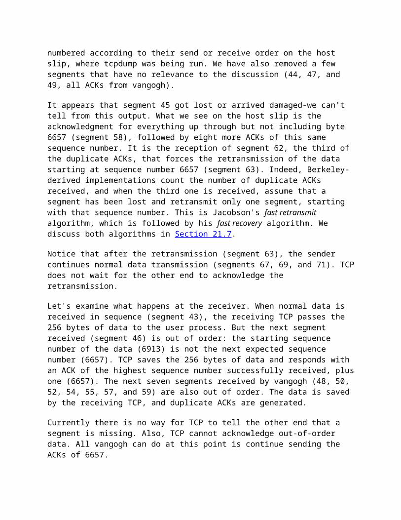
c. Fortran carriage control.The first character of each line is the Fortran format control character.

3. Structure.

a. File structure.(Default) The file is considered as a contiguous stream of bytes. There is no internal file structure.

b. Record structure.This structure is only used with text files (ASCII or EBCDIC).

c. Page structure.Each page is transmitted with a page number to let the receiver store the pages in a random order. Provided by the TOPS-20 operating system. (The Host Requirements RFC recommends against implementing this structure.)

4. Transmission mode. This specifies how the file is transferred across the data connection.

a. Stream mode.(Default) The file is transferred as a stream of bytes. For a file structure, the end-of-file is indicated by the sender closing the data connection. For a record structure, a special 2-byte sequence indicates the end-of-record and end-of-file.

b. Block mode.The file is transferred as a series of blocks, each preceded by one or more header bytes.

c. Compressed mode.A simple run-length encoding compresses consecutive appearances of the same byte. In a text file this would commonly compress strings of blanks, and in a binary file this would commonly compress strings of 0 bytes. (This is rarely used or supported. There are better ways to compress files for FTP.)

If we calculate the number of combinations of all these choices, there could be 72 different ways to transfer and store a file. Fortunately we can ignore many of the options, because they are either antiquated or not supported by most implementations.

Common Unix implementations of the FTP client and server restrict us to the following choices:

Type: ASCII or image. Format control: nonprint only.

Structure: file structure only

Transmission mode: stream mode only.

This limits us to one of two modes: ASCII or image (binary).

This implementation meets the minimum requirements of the Host Requirements RFC. (This RFC also requires support for the record structure, but only if the operating system supports it, which Unix doesn't.)

Many non-Unix implementations provide FTP capabilities to handle their own file formats. The Host Requirements RFC states "The FTP protocol includes many features, some of which are not commonly implemented. However, for every feature in FTP, there exists at least one implementation."

FTP Commands

The commands and replies sent across the control connection between the client and server are in NVT ASCII. This requires a CR, LF pair at the end of each line (i.e., each command or each reply).

The only Telnet commands (those that begin with IAC) that can be sent by the client to the server are interrupt process (<IAC, IP>) and the Telnet synch signal (<IAC, DM> in urgent mode). We'll see that these two Telnet commands are used to abort a file transfer that is in progress, or to query the server while a transfer is in progress. Additionally, if the server receives a Telnet option command from the client (WILL, WONT, DO, or DONT) it responds with either DONT or WONT.

The commands are 3 or 4 bytes of uppercase ASCII characters, some with optional arguments. More than 30 different FTP commands can be sent by the client to the server. Figure 27.2 shows some of the commonly used commands, most of which we'll encounter in this chapter.

Command Description

ABOR LIST filelistPASS passwordPORT n1,n2,n3,n4,n5,n6QUITRETR filenameSTOP filenameSYSTTYPE typeUSER username

abort previous FTP command and any data transferlist files or directoriespassword on serverclient IP address (nl.n2.n3.n4) and port (n5 x 256 + n6)logoff from serverretrieve (get) a filestore (put) a fileserver returns system typespecify file type: A for ASCII, I for imageusemame on server

Figure 27.2 Common FTP commands.

We'll see in the examples in the next section that sometimes there is a one-to-one correspondence between what the interactive user types and the FTP command sent

across the control connection, but for some operations a single user command results in multiple FTP commands across the control connection.

FTP Replies

The replies are 3-digit numbers in ASCII, with an optional message following the number. The intent is that the software needs to look only at the number to determine how to process the reply, and the optional string is for human consumption. Since the clients normally output both the numeric reply and the message string, an interactive user can determine what the reply says by just reading the string (and not have to memorize what all the numeric reply codes mean).

Each of the three digits in the reply code has a different meaning. (We'll see in Chapter 28 that the Simple Mail Transfer Protocol, SMTP, uses the same conventions for commands and replies.)

Figure 27.3 shows the meanings of the first and second digits of the reply code.

Reply Description

1yzPositive preliminary reply. The action is being started but expect another reply before sending another command

2yz Positive completion reply A new command can be sent

3yzPositive intermediate reply. The command has been accepted but another command must be sent

4yzTransient negative completion reply The requested action did not take place, but the error condition is temporary so the command can be reissued later.

5yzPermanent negative completion reply. The command was not accepted and should not be retried.

X0z Syntax errors.

x1z Information.

x2z Connections. Replies referring to the control or data connections.

x3z Authentication and accounting. Replies for the login or accounting commands.

x4z Unspecified.

x5z Filesystem status.

Figure 27.3 Meanings of first and second digits of 3-digit reply codes.

The third digit gives additional meaning to the error message. For example, here are some typical replies, along with a possible message string.

125Data connection already open; transfer starting. 200 Command OK.

214 Help message (for human user).

331 Username OK, password required.

425 Can't open data connection.

452 Error writing file.

500 Syntax error (unrecognized command).

501 Syntax error (invalid arguments).

502 Unimplemented MODE type.

Normally each FTP command generates a one-line reply For example, the QUIT command could generate the reply:

221 Goodbye.

If a multiline reply is needed, the first line contains a hyphen instead of a space after the 3-digit reply code, and the final line contains the same 3-digit reply code, followed by a space. For example, the HELP command could generate the reply:

214- The following commands are recognized (* =>'s unimplemented). USER PORT STOR MSAM* RNTO NLST MKD CDUP PASS PASV APPE MRSQ* ABOR SITE XMKD XCUP ACCT* TYPE MLFL* MRCP* DELE SYST RMD STOU SMNT* STRU MAIL* ALLO CWD STAT XRMD SIZE REIN* MODE MSND* REST XCWD HELP PWD MDTM QUIT RETR MSOM* RNFR LIST NOOP XPWD214 Direct comments to ftp-bugs@bsdi.tuc.noao.edu.

Connection Management

There are three uses for the data connection.

1. Sending a file from the client to the server. 2. Sending a file from the server to the client.

3. Sending a listing of files or directories from the server to the client.

The FTP server sends file listings back across the data connection, rather than as multiline replies across the control connection. This avoids any line limits that restrict the size of a directory listing and makes it easier for the client to save the output of a directory listing into a file, instead of printing the listing to the terminal.

We've said that the control connection stays up for the duration of the client-server connection, but the data connection can come and go, as required. How are the port numbers chosen for the data connection, and who does the active open and passive open?

First, we said earlier that the common transmission mode (under Unix the only transmission mode) is the stream mode, and that the end-of-file is denoted by closing the data connection. This implies that a brand new data connection is required for every file transfer or directory listing. The normal procedure is as follows:

1. The creation of the data connection is under control of the client, because it's the client that issues the command that requires the data connection (get a file, put a file, or list a directory).

2. The client normally chooses an ephemeral port number on the client host for its end of the data connection. The client issues a passive open from this port.

3. The client sends this port number to the server across the control connection using the PORT command.

4. The server receives the port number on the control connection, and issues an active open to that port on the client host. The server's end of the data connection always uses port 20.

Figure 27.4 shows the state of the connections while step 3 is being performed. We assume the client's ephemeral port for the control connection is 1173, and the client's ephemeral port for the data connection is 1174. The command sent by the client is the PORT command and its arguments are six decimal numbers in ASCII, separated by commas. The first four numbers specify the IP address on the client that the server should issue the active open to (140.252.13.34 in this example), and the next two specify the 16-bit port number. Since the 16-bit port number is formed from two numbers, its value in this example is 4 x 256 +150 = 1174.

Figure 27.4 PORT command going across FTP control connection.

Figure 27.5 shows the state of the connection when the server issues the active open to the client's end of the data connection. The server's end point is at port 20.

Figure 27.5 FTP server doing active open of data connection.

The server always does the active open of the data connection. Normally the server also does the active close of the data connection, except when the client is sending a tile to the server in stream mode, which requires the client to close the connection (which gives the server the end-of-tile notification).

It is also possible for the client to not issue the PORT command, in which case the server issues the active open to the same port number being used by the client for its end of the control connection (1173 in this example). This is OK, since the server's port numbers for the two connections are different: one is 20 and the other is 21. Nevertheless, in the next section we'll see why current implementations normally don't do this.

27.3 FTP Examples

We now look at some examples using FTP: its management of the data connection, how text files are sent using NVT ASCII, FTP'S use of the Telnet synch signal to abort an inprogress transfer, and finally the popular "anonymous FTP."

Connection Management: Ephemeral Data Port

Let's first look at FTP's connection management with a simple FTP session that just lists a file on the server. We run the client on the host svr4 with the -d flag (debug). This tells it to print the commands and replies that are exchanged across the control connection. All the lines preceded by ---> are sent by the client to the server, and the lines that begin with a 3-digit number are the server's replies. The client's interactive prompt is ftp>.

svr4 % ftp -d bsdi -d option for debug output Connected to bsdi. client does active open of control connection 220 bsdi FTP server (Version 5.60) ready. server responds it is ready Name (bsdi:rstevens): client prompts us for a login name ---> USER rstevens we type RETURN, so client sends default 331 Password required for rstevens. Password: we type our password; it's not echoed ---> PASS XXXXXXX client sends it as cleartext 230 User rstevens logged in. ftp> dir hello.c ask for directory listing of a single file ---> PORT 140,252,13,34,4,150 see figure 27.4 200 PORT command successful.

---> LIST hello.c 150 Opening ASCII mode data connection for /bin/ls. -rw-r--r-- 1 rstevens staff 38 Jul 17 12:47 hello.c 226 Transfer complete. remote: hello.c output by client 56 bytes received in 0.03 seconds (1.8 Kbytes/s) ftp> quit we're done---> QUIT 221 Goodbye.

When the FTP client prompts us for a login name, it prints the default (our login name on the client). When we type the RETURN key, this default is sent.

Asking for a directory listing of a single file causes a data connection to be established and used. This example follows the procedure we showed in Figures 27.4 and 27.5. The client asks its TCP for an ephemeral port number for its end of the data connection, and sends this port number (1174) to the server in a PORT command. We can also see that a single interactive user command (dir) becomes two FTP commands (PORT and LIST).

Figure 27.6 is the time line of the packet exchange across the control connection. (We have removed the establishment and termination of the control connection, along with all the window size advertisements.) We note in this figure where the data connection is opened, used, and then closed.

Figure 27.6 Control connection for FTP example.

Figure 27.7 is the time line for the data connection. The times in this figure are from the same starting point as Figure 27.6. We have removed all window advertisements, but have left in the type-of-service field, to show that the data connection uses a different type-of-service (maximize throughput) than the control connection (minimize delay). (The TOS values are in Figure 3.2.)

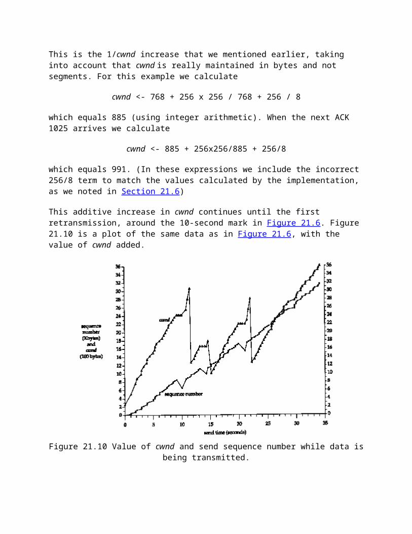
Figure 27.7 Data connection for FTP example.

In this time line the FTP server does the active open of the data connection, from port 20 (called ftp-data), to the port number from the PORT command (1174). Also in this example, where the server writes to the data connection, the server does the active close of the data connection, which tells the client when the listing is complete.

Connection Management: Default Data Port

If the client does not send a PORT command to the server, to specify the port number for the client's end of the data connection, the server uses the same port number for the data connection that is being used for the control connection. This can cause problems for clients that use the stream mode (which the Unix FTP clients and server always use), as we show below.

The Host Requirements RFC recommends that an FTP client using the stream mode send a PORT command to use a nondefault port number before each use of the data connection.

Returning to the previous example (Figure 27.6), what if we asked for another directory listing a few seconds after the first? The client would ask its kernel to choose another ephemeral port number (perhaps 1175) and the next data connection would be between svr4 port 1175 and bsdi port 20. But in Figure 27.7 the server did the active close of the data connection, and we showed in Section 18.6 that the server won't be able to assign port 20 to the new data connection, because that local port number was used by an earlier connection that is still in the 2MSL wait state.

The server gets around this by specifying the SO_REUSEADDR option that we mentioned in Section 18.6. This lets it assign port 20 to the new connection, and the new connection will have a different foreign port number (1175) from the one that's in the 2MSL wait (1174), so everything is OK.

This scenario changes if the client does not send the PORT command, specifying an ephemeral port number on the client. We can force this to happen by executing the user command sendport to the FTP client. Unix FTP clients use this command to turn off sending PORT commands to the server before each use of a data connection.

Figure 27.8 shows the time line only for the data connections for two consecutive LIST commands. The control connection originates from port 1176 on host svr4, so in the absence of PORT commands, the client and server use this same port number for the data connection. (We have removed the window advertisements and type-of-service values.)

Figure 27.8 Data connection for two consecutive LIST commands.

The sequence of events is as follows.

1. The control connection is established from the client port 1176 to the server port 21. (We don't show this.)

2. When the client does the passive open for the data connection on port 1176, it must specify the SO_REUSEADDR option since that port is already in use by the control connection on the client.

3. The server does the active open of the data connection (segment 1) from port 20 to port 1176. The client accepts this (segment 2), even though port 1176 is already in use on the client, because the two socket pairs

<svr4, 1176, bsdi, 21><svr4, 1176, bsdi, 20>

are different (the port numbers on bsdi are different). TCP demultiplexes incoming segments by looking at the source IP address, source port number, destination IP address, and destination port number, so as long as one of the four elements differs, all is OK.

4. The server does the active close of the data connection (segment 5), which puts the socket pair

<svr4, 1176, bsdi, 20>

in a 2MSL wait on the server.

5. The client sends another LIST command across the control connection. (We don't show this.) Before doing this the client does a passive open on port 1176 for its end of the data connection. The client must specify the SO_REUSEADDR option again, since the port number 1176 is already in use.

6. The server issues an active open for the data connection from port 20 to port 1176. Before doing this the server must specify SO_REUSEADDR, since the local port (20) is associated with a connection that is in the 2MSL wait, but from what we showed in Section 18.6, the connection won't succeed. The reason is that the socket pair for the connection request equals the socket pair from step 4 that is still in a 2MSL wait. The rules of TCP forbid the server from sending the SYN. There is no way for the server to override this 2MSL wait of the socket pair before reusing the same socket pair.

At this point the BSD server retries the connection request every 5 seconds, up to 18 times, for a total of 90 seconds. We see that segment 9 succeeds about 1 minute later. (We mentioned in Chapter 18 that SVR4 uses an MSL of 30 seconds, for a 2MSL wait of 1 minute.) We don't see any SYNs from these failures in this time line because the active opens fail and the server's TCP doesn't even send a SYN.

The reason the Host Requirements RFC recommends using the PORT command is to avoid this 2MSL wait between successive uses of a data connection. By continually changing the port number on one end, the problem we just showed disappears.

Text File Transfer: NVT ASCII Representation or Image?

Let's verify that the transmission of a text file uses NVT ASCII by default. This time we don't specify the -d flag, so we don't see the client commands, but notice that the client still prints the server's responses:

sun % ftp bsdi Connected to bsdi.220 bsdi FTP server (Version 5.60) ready. Name (bsdi:rstevens): we type RETURN 331 Password required for rstevens. Password: we type our password 230 User rstevens logged in.ftp> get hello.c fetch a file200 PORT command successful.150 Opening ASCII mode data connection for hello.c (38 bytes). 226 Transfer complete. server says file contains 38 bytes local: hello.c remote: hello.c output by client42 bytes received in 0.0037 seconds (11 Kbytes/s) 42 bytes across data connection ftp> quit 221 Goodbye.sun % ls -l hello.c -rw-rw-r-1 rstevens 38 Jul 18 08:48 hello.c but file contains 38 bytes sun % wc -l hello.c count the lines in the file 4 hello.c

Forty-two bytes are transferred across the data connection because the file contains four lines. Each Unix newline character (\n) is converted into the NVT ASCII 2-byte end-of-line sequence (\r\n) by the server for transmission, and then converted back by the client for storage.

Newer clients attempt to determine if the server is of the same system type, and if so, transfer files in binary (image file type) instead of ASCII. This helps in two ways.

1. The sender and receiver don't have to look at every byte (a big savings). 2. Fewer bytes are transferred if the host operating system uses fewer bytes for the

end-of-line than the 2-byte NVT ASCII sequence (a smaller savings).

We can see this optimization using a BSD/386 client and server. We'll enable the debug mode, to see the client FTP commands:

bsdi % ftp -d slip specify -d to see client commands Connected to slip.

220 slip FTP server (Version 5.60) ready. Name (slip:rstevens): we type RETURN---> USER rstevens 331 Password required for rstevens. Password: we type our password ---> PASS XXXX 230 User rstevens logged in. ---> SYST this is sent automatically by client 215 UNIX Type: L8 Version: BSD-199103 server's replyRemote system type is UNIX. information output by client Using binary mode to transfer files. information output by client ftp> get hello.c fetch a file---> TYPE I sent automatically by client 200 Type set to I. ---> PORT 140,252,13,66,4,84 port number=4x256+84=1108 200 PORT command successful. ---> RETR hello.c 150 Opening BINARY mode data connection for hello.c (38 bytes). 226 Transfer complete. 38 bytes received in 0.035 seconds (1.1 Kbytes/s) only 38 bytes this timeftp> quit ---> QUIT221 Goodbye.

After we login to the server, the client FTP automatically sends the SYST command, which the server responds to with its system type. If the reply begins with the string "215 UNIX Type: L8", and if the client is running on a Unix system with 8 bits per byte, binary mode (image) is used for all file transfers, unless changed by the user.

When we fetch the file hello.c the client automatically sends the command TYPE I to set the file type to image. Only 38 bytes are transferred across the data connection.

The Host Requirements RFC says an FTP server must support the SYST command (it was an option in RFC 959). But the only systems used in the text (see inside front cover) that support it are BSD/386 and AIX 3.2.2. SunOS 4.1.3 and Solaris 2.x reply with 500 (command not understood). SVR4 has the extremely unsocial behavior of replying with 500 and closing the control connection!

Aborting A File Transfer: Telnet Synch Signal

We now look at how the FTP client aborts a file transfer from the server. Aborting a file transfer from the client to the server is easy - the client stops sending data across the data connection and sends an ABOR to the server on the control connection. Aborting a receive,

however, is more complicated, because the client wants to tell the server to stop sending data immediately. We mentioned earlier that the Telnet synch signal is used, as we'll see in this example.

We'll initiate a receive and type our interrupt key after it has started. Here is the interactive session, with the initial login deleted:

ftp> get a.out fetch a large file ---> TYPE I client and server are both 8-bit byte Unix systems 200 Type set to I.---> PORT 140,252,13,66,4,99200 PORT command successful.---> RETR a.out150 Opening BINARY mode data connection for a.out (28672 bytes). ^? type our interrupt key receive aborted output by client waiting for remote to finish abort output by client 426 Transfer aborted. Data connection closed. 226 Abort successful1536 bytes received in 1.7 seconds (0.89 Kbytes/s)

After we type our interrupt key, the client immediately tells us it initiated the abort and is waiting for the server to complete. The server sends two replies: 426 and 226. Both replies are sent by the Unix server when it receives the urgent data from the client with the ABOR command.

Figures 27.9 and 27.10 show the time line for this session. We have combined the control connection (solid lines) and the data connection (dashed lines) to show the relationship between the two.

Figure 27.9 Aborting a file transfer (first half).

The first 12 segments in Figure 27.9 are what we expect. The commands and replies across the control connection set up the file transfer, the data connection is opened, and the first segment of data is sent from the server to the client.

Figure 27.10 Aborting a file transfer (second half).

In Figure 27.10, segment 13 is the receipt of the sixth data segment from the server on the data connection, followed by segment 14, which is generated by our typing the interrupt key. Ten bytes are sent by the client to abort the transfer:

<IAC, IP, IAC, DM, A, B, O, R, \r, \n>

We see two segments (14 and 15) because of the problem we detailed in Section 20.8 dealing with TCP's urgent pointer. (We saw the same handling of this problem in Figure 26.17 with Telnet.) The Host Requirements RFC says the urgent pointer should point to the last byte of urgent data, while most Berkeley-derived implementations have it point 1 byte beyond the last byte of urgent data. The FTP client purposely writes the first 3 bytes as urgent data, knowing the urgent pointer will (incorrectly) point to the next byte that is written (the data mark, DM, at sequence number 54). This first write with 3 bytes of urgent data is sent immediately, along with the urgent pointer, followed by the next 7 bytes. (The BSD FTP server does not have a problem with which interpretation of the urgent pointer is

used by the client. When the server receives urgent data on the control connection it reads the next FTP command, looking for ABOR or STAT, ignoring any embedded Telnet commands.)

Notice that despite the server saying the transfer was aborted (segment 18, on the control connection), the client receives 14 more segments of data (sequence numbers 1537 through 5120) on the data connection. These segments were probably queued in the network device driver on the server when the abort was received, but the client prints "1536 bytes received" meaning it ignores all the segments of data that it receives (segments 17 and later) after sending the abort (segments 14 and 15).

In the case of a Telnet user typing the interrupt key, we saw in Figure 26.17 that by default the Unix client does not send the interrupt process command as urgent data. We said this was OK because there is little chance that the flow of data from the client to the server is stopped by flow control. With FTP the client is also sending an interrupt process command across the control connection, and since two connections are being used there is little chance that the control connection is stopped by flow control. Why does FTP send the interrupt process command as urgent data when Telnet does not? The answer is that FTP uses two connections, whereas Telnet uses one, and on some operating systems it may be hard for a process to monitor two connections for input at the same time. FTP assumes that these marginal operating systems at least provide notification that urgent data has arrived on the control connection, allowing the server to then switch from handling the data connection to the control connection.

Anonymous FTP

One form of FTP is so popular that we'll show an example of it. It's called anonymous FTP, and when supported by a server, allows anyone to login and use FTP to transfer files. Vast amounts of free information are available using this technique.

How to find which site has what you're looking for is a totally different problem. We mention it briefly in Section 30.4.

We'll use anonymous FTP to the site ftp.uu.net (a popular anonymous FTP site) to fetch the errata file for this book. To use anonymous FTP we login with the username of "anonymous" (you learn to spell it correctly after a few times). When prompted for a password we type our electronic mail address.

sun % ftp ftp.uu.net Connected to ftp.uu.net.220 ftp.UU.NET FTP server (Version 2.0WU(13) Fri Apr 9 20:44:32 EDT 1993) ready. Name (ftp.uu.net:rstevens): anonymous 331 Guest login ok, send your complete e-mail address as password. Password: we type rstevens@noao.edu; it's not echoed 230-230- Welcome to the UUNET archive.

230- A service of UUNET Technologies Inc, Falls Church, Virginia 230- For information about UUNET, call +1 703 204 8000, or see the files 230- in /uunet-info

more greeting lines 230 Guest login ok, access restrictions apply. ftp> cd published/books change to the desired directory 250 CWD command successful.ftp> binary we'll transfer a binary file 200 Type set to I.ftp> get stevens.tcpipivl.errata.Z fetch the file200 PORT command successful.150 Opening BINARY mode data connection for stevens.tcpipivl.errata.Z (105 bytes). 226 Transfer complete, (you may get a different file size) local: stevens.tcpipivl.errata.Z remote: stevens.tcpipivl.errata.Z 105 bytes received in 4.1 seconds (0.83 Kbytes/s) ftp> quit 221 Goodbye.sun % uncompress stevens.tcpipivl.errata.Z sun % more stevens.tcpipivl.errata

The uncompress is because many files available for anonymous FTP are compressed using the Unix compress(l) program, resulting in a file extension of .Z. These files must be transferred using the binary file type, not the ASCII file type.

Anonymous FTP from an Unknown IP Address

We can tie together some features of routing and the Domain Name System using anonymous FTP. In Section 14.5 we talked about pointer queries in the DNS - taking an IP address and returning the hostname. Unfortunately not all system administrators set up their name servers correctly with regard to pointer queries. They often add new hosts to the file required for name-to-address mapping, but forget to add them to the file for address-to-name mapping. We often see this with traceroute, when it prints an IP address instead of a hostname.

Some anonymous FTP servers require that the client have a valid domain name. This allows the server to log the domain name of the host that's doing the transfer. Since the only client identification the server receives in the IP datagram from the client is the IP address of the client, the server can call the DNS to do a pointer query, and obtain the domain name of the client. If the name server responsible for the client host is not set up correctly, this pointer query can fail. To see this error we'll do the following steps.

1. Change the IP address of our host slip (see the figure on the inside front cover) to 140.252.13.67. This is a valid IP address for the author's subnet, but not entered into the name server for the noao.edu domain.

2. Change the destination IP address of the SLIP link on bsdi to 140.252.13.67.

3. Add a routing table entry on sun that directs datagrams for 140.252.13.67 to the router bsdi. (Recall our discussion of this routing table in Section 9.2.)

Our host slip is still reachable across the Internet, because we saw in Section 10.4 that the routers gateway and netb just sent any datagram destined for the subnet 140.252.13 to the router sun. Our router sun knows what to do with these datagrams from the routing table entry we made in step 3 above. What we have created is a host with complete Internet connectivity, but without a valid domain name. That is, a pointer query for the IP address 140.252.13.67 will fail.

We now use anonymous FTP to a server that we know requires a valid domain name:

slip % ftp ftp.uu.net Connected to ftp.uu.net.220 ftp.UU.NET FTP server (Version 2.0WU(13) Fri Apr 9 20:44:32 EDT 1993) ready. Name (ftp.uu.net:rstevens): anonymous 530- Sorry, we're unable to map your IP address 140.252.13.67 to a hostname 530- in the DNS. This is probably because your nameserver does not have a 530- PTR record for your address in its tables, or because your reverse 530- nameservers are not registered. We refuse service to hosts whose 530- names we cannot resolve. If this is simply because your nameserver is 530- hard to reach or slow to respond then try again in a minute or so, and 530- perhaps our nameserver will have your hostname in its cache by then. 530- If not, try reaching us from a host that is in the DNS or have your 530- system administrator fix your servers. 530 User anonymous access denied.. Login failed.Remote system type is UNIX.Using binary mode to transfer files. ftp> quit 221 Goodbye.

The error reply from the server is self-explanatory.

NFS: Network File System

29.1 Introduction

In this chapter we describe NFS, the Network File System, another popular application that provides transparent file access for client applications. The building block of NFS is Sun RPC: Remote Procedure Call, which we must describe first.

Nothing special need be done by the client program to use NFS. The kernel detects that the file being accessed is on an NFS server and automatically generates the RPC calls to access the file.

Our interest in NFS is not in all the details on file access, but in its use of the Internet protocols, especially UDP.

29.2 Sun Remote Procedure Call

Most network programming is done by writing application programs that call system-provided functions to perform specific network operations. For example, one function performs a TCP active open, another performs a TCP passive open, another sends data across a TCP connection, another sets specific protocol options (enable TCP's keepalive timer), and so on. In Section 1.15 we mentioned that two popular sets of functions for network programming (called APIs) are sockets and TLI. The API used by the client and the API used by the server can be different, as can the operating systems running on the client and server. It is the communication protocol and application protocol that determine if a given client and server can communicate with each other. A Unix client written in C using sockets and TCP can communicate with a mainframe server written in COBOL using some other API and TCP, if both hosts are connected across a network and both have a TCP/IP implementation.

Typically the client sends commands to the server, and the server sends replies back to the client. All the applications we've looked at so far - Ping, Traceroute, routing daemons, and the clients and servers for the DNS, TFTP, BOOTP, SNMP, Telnet, FTP, and SMTP-are built this way.

RPC, Remote Procedure Call, is a different way of doing network programming. A client program is written that just calls functions in the server program. This is how it appears to the programmer, but the following steps actually take place.

1. When the client calls the remote procedure, it's really calling a function on the local host that's generated by the RPC package. This function is called the client stub. The client stub packages the procedure arguments into a network message, and sends this message to the server.

2. A server stub on the server host receives the network message. It takes the arguments from the network message, and calls the server procedure that the application programmer wrote.

3. When the server function returns, it returns to the server stub, which takes the return values, packages them into a network message, and sends the message back to the client stub.

4. The client stub takes the return values from the network message and returns to the client application.

The network programming done by the stubs and the RPC library routines uses an API such as sockets or TLI, but the user application-the client program, and the server procedures called by the client-never deal with this API. The client application just calls the server procedures and all the network programming details are hidden by the RPC package, the client stub, and the server stub. An RPC package provides numerous benefits.

1. The programming is easier since there is little or no network programming involved. The application programmer just writes a client program and the server procedures that the client calls.

2. If an unreliable protocol such as UDP is used, details like timeout and retransmission are handled by the RPC package. This simplifies the user application.

3. The RPC library handles any required data translation for the arguments and return values. For example, if the arguments consist of integers and floating point numbers, the RPC package handles any differences in the way integers and floating point numbers are stored on the client and server. This simplifies coding clients and servers that can operate in heterogeneous environments.

Details of RPC programming are provided in Chapter 18 of [Stevens 1990]. Two popular RPC packages are Sun RPC and the RPC package in the Open Software Foundation's (OSF) Distributed Computing Environment (DCE). Our interest in RPC is to see what the procedure call and procedure return messages look like for the Sun RPC package, since it's used by the Network File System, which we describe in this chapter. Version 2 of Sun RPC is defined in RFC 1057 [Sun Microsystems 1988a].

Sun RPC

Sun RPC comes in two flavors. One version is built using the sockets API and works with TCP and UDP. Another, called TI-RPC (for "transport independent"), is built using the TLI API and works with any transport layer provided by the kernel. From our perspective the two are the same, although we talk only about TCP and UDP in this chapter.

Figure 29.1 shows the format of an RPC procedure call message, when UDP is used.

Figure 29.1 Format of RPC procedure call message as a UDP datagram.

The IP and UDP headers are the standard ones we showed earlier (Figures 3.1 and 11.2). What follows after the UDP header is defined by the RPC package.

The transaction ID (XID) is set by the client and returned by the server. When the client receives a reply it compares the XID returned by the server with the XID of the request it sent. If they don't match, the client discards the message and waits for the next one from the server. Each time the client issues a new RPC, it changes the XID. But if the client retransmits a previously sent RPC (because it hasn't received a reply), the XID does not change.

The call variable is 0 for a call, and 1 for a reply. The current RPC version is 2. The next three variables, program number, version number, and procedure number, identify the specific procedure on the server to be called.

The credentials identify the client. In some instances nothing is sent here, and in other instances the numeric user ID and group IDs of the client are sent. The server can look at the credentials and determine if it will perform the request or not. The verifier is used with Secure RPC, which uses DES encryption. Although the credentials and verifier are variable-length fields, their length is encoded as part of the field.

Following this are the procedure parameters. The format of these depends on the definition of the remote procedure by the application. How does the receiver (the server stub) know

the size of the parameters? Since UDP is being used, the size of the UDP datagram, minus the length of all the fields up through the verifier, is the size of the parameters. When TCP is used instead of UDP, there is no inherent length, since TCP is a byte stream protocol, without record boundaries. To handle this, a 4-byte length field appears between the TCP header and the XID, telling the receiver how many bytes comprise the RPC call. This allows the RPC call message to be sent in multiple TCP segments, if necessary. (The DNS uses a similar technique; see Exercise 14.4.)

Figure 29.2 shows the format of an RPC reply. This is sent by the server stub to the client stub, when the remote procedure returns.

Figure 29.2 Format of RPC procedure reply message as a UDP datagram.

The XID in the reply is just copied from the XID in the call. The reply is 1, which we said differentiates this message from a call. The status is 0 if the call message was accepted. (The message can be rejected if the RPC version number isn't 2, or if the server cannot authenticate the client.) The verifier is used with secure RPC to identify the server.

The accept status is 0 on success. A nonzero value can indicate an invalid version number or an invalid procedure number, for example. As with the RPC call message, if TCP is used instead of UDP, a 4-byte length field is sent between the TCP header and the XID.

29.3 XDR: External Data Representation

XDR, External Data Representation, is the standard used to encode the values in the RPC call and reply messages-the RPC header fields (XID, program number, accept status, etc.), the procedure parameters, and the procedure results. Having a standard way of encoding all these values is what lets a client on one system call a procedure on a system with a different architecture. XDR is defined in RFC 1014 [Sun Microsystems 1987].

XDR defines numerous data types and exactly how they are transmitted in an RPC message (bit order, byte order, etc.). The sender must build an RPC message in XDR format, then the receiver converts the XDR format into its native representation. We see, for example, in Figures 29.1 and 29.2, that all the integer values we show (XID, call, program number, etc.) are 4-byte integers. Indeed, all integers occupy 4 bytes in XDR. Other data types supported by XDR include unsigned integers, booleans, floating point numbers, fixed-length arrays, variable-length arrays, and structures.

29.4 Port Mapper

The RPC server programs containing the remote procedures use ephemeral ports, not well-known ports. This requires a "registrar" of some form that keeps track of which RPC programs are using which ephemeral ports. In Sun RPC this registrar is called the port mapper.

The term "port" in this name originates from the TCP and UDP port numbers, features of the Internet protocol suite. Since TI-RPC works over any transport layer, and not just TCP and UDP, the name of the port mapper in systems using TI-RPC (SVR4 and Solaris 2.2, for example) has become rpcbind. We'll continue to use the more familiar name of port mapper.

Naturally, the port mapper itself must have a well-known port: UDP port 111 and TCP port 111. The port mapper is also just an RPC server program. It has a program number (100000), a version number (2), a TCP port of 111, and a UDP port of 111. Servers register themselves with the port mapper using RPC calls, and clients query the port mapper using RPC calls. The port mapper provides four server procedures:

1. PMAPPROC_SET. Called by an RPC server on startup to register a program number, version number, and protocol with a port number.

2. PMAPPROCJJNSET. Called by server to remove a previously registered mapping.

3. PMAPPROC_GETPORT. Called by an RPC client on startup to obtain the port number for a given program number, version number, and protocol.

4. PMAPPROC_DUMP. Returns all entries (program number, version number, protocol, and port number) in the port mapper database.

When an RPC server program starts, and is later called by an RPC client program, the following steps take place.

1. The port mapper must be started first, normally when the system is bootstrapped. It creates a TCP end point and does a passive open on TCP port 111. It also creates a UDP end point and waits for a UDP datagram to arrive for UDP port 111.

2. When the RPC server program starts, it creates a TCP end point and a UDP end point for each version of the program that it supports. (A given RPC program can support multiple versions. The client specifies which version it wants when it calls a server

procedure.) An ephemeral port number is bound to both end points. (It doesn't matter whether the TCP port number is the same or different from the UDP port number.) The server registers each program, version, protocol, and port number by making a remote procedure call to the port mapper's PMAPPROC_SET procedure.

3. When the RPC client program starts, it calls the port mapper's PMAP-PROC_GETPORT procedure to obtain the ephemeral port number for a given program, version, and protocol.

4. The client sends an RPC call message to the port number returned in step 3. If UDP is being used, the client just sends a UDP datagram containing an RPC call message (Figure 29.1) to the server's UDP port number. The server responds by sending a UDP datagram containing an RPC reply message (Figure 29.2) back to the client.

If TCP is being used, the client does an active open to the server's TCP port number, and then sends an RPC call message across the connection. The server responds with an RPC reply message across the connection.

The program rpcinfo(8) prints out the port mapper's current mappings. (It calls the port mapper's PMAPPROC_DUMP procedure.) Here is some typical output:

sun % /usr/etc/rpcinfo -p program vers proto port 100005 1 tcp 702 mountd mount daemon for NFS 100005 1 udp 699 mountd100005 2 tcp 702 mountd100005 2 udp 699 mountd 100003 2 udp 2049 nfs NFS itself 100021 1 tcp 709 niockmgr NFS lock manager 100021 1 udp 1036 niockmgr100021 2 tcp 721 niockmgr100021 2 udp 1039 niockmgr100021 3 tcp 713 niockmgr 100021 3 udp 1037 niockmgr

We see that some programs do support multiple versions, and each combination of a program number, version number, and protocol has its own port number mapping maintained by the port mapper.

Both versions of the mount daemon are accessed through the same TCP port number (702) and the same UDP port number (699), but each version of the lock manager has its own port number.

29.5 NFS Protocol

NFS provides transparent file access for clients to files and filesystems on a server. This differs from FTP (Chapter 27), which provides file transfer. With FTP a complete copy of the file is made. NFS accesses only the portions of a file that a process references, and a goal of NFS is to make this access transparent. This means that any client application that works with a local tile should work with an NFS file, without any program changes whatsoever.

NFS is a client-server application built using Sun RPC. NFS clients access tiles on an NFS server by sending RPC requests to the server. While this could be done using normal user processes - that is, the NFS client could be a user process that makes explicit RPC calls to the server, and the server could also be a user process-NFS is normally not implemented this way for two reasons. First, accessing an NFS tile must be transparent to the client. Therefore the NFS client calls are performed by the client operating system, on behalf of client user processes. Second, NFS servers are implemented within the operating system on the server for efficiency. If the NFS server were a user process, every client request and server reply (including the data being read or written) would have to cross the boundary between the kernel and the user process, which is expensive.

In this section we look at version 2 of NFS, as documented in RFC 1094 [Sun Microsystems 1988b]. A better description of Sun RPC, XDR, and NFS is given in [X/Open 1991]. Details on using and administering NFS are in [Stern 1991]. The specifications for version 3 of the NFS protocol were released in 1993, which we cover in Section 29.7.

Figure 29.3 shows the typical arrangement of an NFS client and an NFS server. There are many subtle points in this figure.

Figure 29.3 Typical arrangement of NFS client and NFS server.1. It is transparent to the client whether it's accessing a local file or an NFS file. The

kernel determines this when the file is opened. After the tile is opened, the kernel passes all references to local tiles to the box labeled "local file access," and all references to an NFS tile are passed to the "NFS client" box.

2. The NFS client sends RPC requests to the NFS server through its TCP/IP module. NFS is used predominantly with UDP, but newer implementations can also use TCP.

3. The NFS server receives client requests as UDP datagrams on port 2049. Although NFS could be made to use the port mapper, allowing the server to use an ephemeral port, UDP port 2049 is hardcoded into most implementations.

4. When the NFS server receives a client request, the requests are passed to its local file access routines, which access a local disk on the server.

5. It can take the NFS server a while to handle a client's request. The local file-system is normally accessed, which can take some time. During this time, the server does not want to block other client requests from being serviced. To handle this, most NFS servers are multithreaded-that is, there are really multiple NFS servers running inside the server kernel. How this is handled depends on the operating system. Since most Unix kernels are not multithreaded, a common technique is to start multiple instances of a user process (often called nfsd) that performs a single system call and remains inside the kernel as a kernel process.

6. Similarly, it can take the NFS client a while to handle a request from a user process on the client host. An RPC is issued to the server host, and the reply is waited for. To provide more concurrency to the user processes on the client host that are using NFS, there are normally multiple NFS clients running inside the client kernel. Again, the implementation depends on the operating system. Unix systems often use a technique similar to the NFS server technique: a user process named biod that performs a single system call and remains inside the kernel as a kernel process.

Most Unix hosts can operate as either an NFS client, an NFS server, or both. Most PC implementations (MS-DOS) only provide NFS client implementations. Most IBM mainframe implementations only provide NFS server functions.

NFS really consists of more than just the NFS protocol. Figure 29.4 shows the various RPC programs normally used with NFS.

ApplicationProgram number

Version numbers

Number ofprocedures

port mapperNFSmountlock managerstatus monitor

100000100003100005100021100024

221

1,2,31

4155

196

Figure 29.4 Various RPC programs used with NFS.

The versions we show in this figure are the ones found on systems such as SunOS 4.1.3. Newer implementations are providing newer versions of some of the programs. Solaris 2.2,

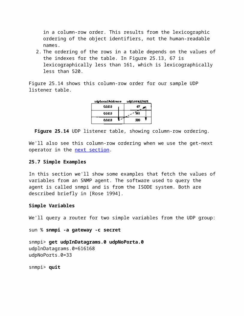
for example, also supports versions 3 and 4 of the port mapper, and version 2 of the mount daemon. SVR4 also supports version 3 of the port mapper.

The mount daemon is called by the NFS client host before the client can access a filesystem on the server. We discuss this below.

The lock manager and status monitor allow clients to lock portions of files that reside on an NFS server. These two programs are independent of the NFS protocol because locking requires state on both the client and server, and NFS itself is stateless on the server. (We say more about NFS's statelessness later.) Chapters 9, 10, and 11 of [X/Open 1991] document the procedures used by the lock manager and status monitor for file locking with NFS.

File Handles

A fundamental concept in NFS is the file handle. It is an opaque object used to reference a file or directory on the server. The term opaque denotes that the server creates the file handle, passes it back to the client, and then the client uses the file handle when accessing the file. The client never looks at the contents of the file handle-its contents only make sense to the server.

Each time a client process opens a file that is really a file on an NFS server, the NFS client obtains a file handle for that file from the NFS server. Each time the NFS client reads or writes that file for the user process, the file handle is sent back to the server to identify the file being accessed.

Normal user processes never deal with file handles - it is the NFS client code and the NFS server code that pass them back and forth. In version 2 of NFS a file handle occupies 32 bytes, although this increases with version 3 to 64 bytes.

Unix servers normally store the following information in the file handle: the filesystem identifier (the major and minor device numbers of the filesystem), the i-node number (a unique number within a filesystem), and an i-node generation number (a number that changes each time an i-node is reused for a different file).

Mount Protocol

The client must use the NFS mount protocol to mount a server's filesystem, before the client can access files on that filesystem. This is normally done when the client is bootstrapped. The end result is for the client to obtain a file handle for the server's file-system.

Figure 29.5 shows the sequence of steps that takes place when a Unix client issues the mount (8) command, specifying an NFS mount.

Figure 29.5 Mount protocol used by Unix mount command.

The following steps take place.

1. The port mapper is started on the server, normally when the server bootstraps. 2. The mount daemon (mountd) is started on the server, after the port mapper. It

creates a TCP end point and a UDP end point, and assigns ephemeral port number to each. It then registers these port numbers with the port mapper.

3. The mount command is executed on the client and it issues an RPC call to the port mapper on the server to obtain the port number of the server's mount daemon. Either TCP or UDP can be used for this client exchange with the port mapper, but UDP is normally used.

4. The port mapper replies with the port number.

5. The mount command issues an RPC call to the mount daemon to mount a file-system on the server. Again, either TCP or UDP can be used, but UDP is typical. The server can now validate the client, using the client's IP address and port number, to see if the server lets this client mount the specified filesystem.

6. The mount daemon replies with the file handle for the given filesystem.

7. The mount command issues the mount system call on the client to associate the file handle returned in step 5 with a local mount point on the client. This file handle is stored in the NFS client code, and from this point on any references by user processes to files on that server's filesystem will use that file handle as the starting point.

This implementation technique puts all the mount processing, other than the mount system call on the client, in user processes, instead of the kernel. The three programs we show-the mount command, the port mapper, and the mount daemon-are all user processes. As an example, on our host sun (the NFS client) we execute

sun # mount -t nfs bsdi:/usr /nfs/bsdi/usr

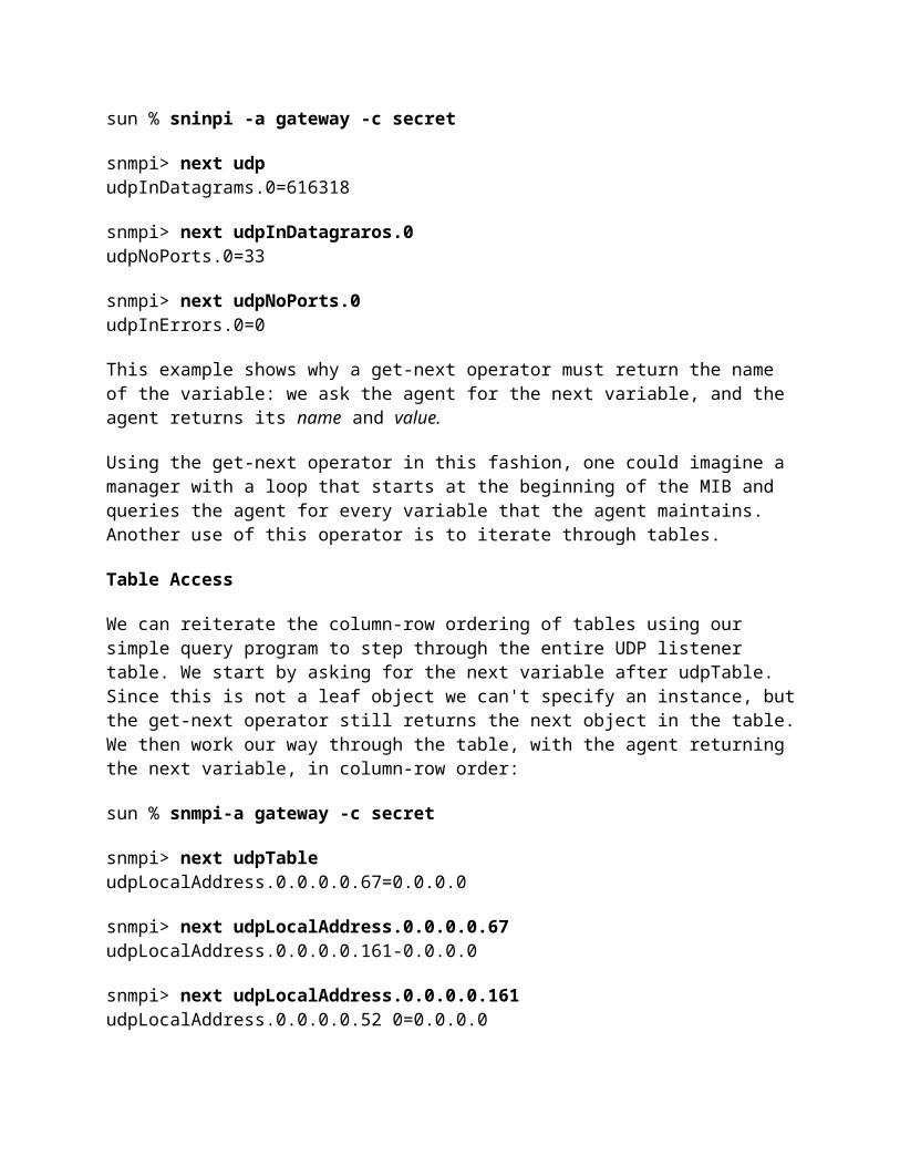
This mounts the directory /usr on the host bsdi (the NFS server) as the local file-system /nfs/bsdi/usr. Figure 29.6 shows the result.

Figure 29.6 Mounting the bsdi:/usr directory as /nfs/bsdi/usr on the host sun.

When we reference the file /nfs/bsdi/usr/rstevens/hello.c on the client sun we are really referencing the file /usr/rstevens/hello.c on the server bsdi.

NFS Procedures

The NFS server provides 15 procedures, which we now describe. (The numbers we use are not the same as the NFS procedure numbers, since we have grouped them according to functionality.) Although NFS was designed to work between different operating systems, and not just Unix systems, some of the procedures provide Unix functionality that might not be supported by other operating systems (e.g., hard links, symbolic links, group owner, execute permission, etc.). Chapter 4 of [Stevens 1992] contains additional information on the properties of Unix filesystems, some of which are assumed by NFS.

1. GETATTR. Return the attributes of a file; type of file (regular file, directory, etc.), permissions, size of file, owner of file, last-access time, and so on.

2. SETATTR. Set the attributes of a file. Only a subset of the attributes can be set: permissions, owner, group owner, size, last-access time, and last-modification time.

3. STATFS. Return the status of a filesystem: amount of available space, optimal size for transfer, and so on. Used by the Unix df command, for example.

4. LOOKUP. Lookup a file. This is the procedure called by the client each time a user process opens a file that's on an NFS server. A file handle is returned, along with the attributes of the file.

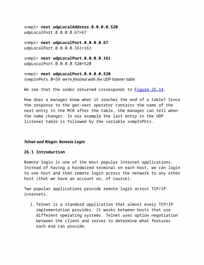
5. READ. Read from a file. The client specifies the file handle, starting byte offset, and maximum number of bytes to read (up to 8192).

6. WRITE. Write to a file. The client specifies the file handle, starting byte offset, number of bytes to write, and the data to write.

7. *NFS writes are required to be synchronous. The server cannot respond OK until it has successfully written the data (and any other file information that gets updated) to disk.

8. CREATE. Create a file.

9. REMOVE. Delete a file.

10. RENAME. Rename a file.

11. LINK. Make a hard link to a file. A hard link is a Unix concept whereby a given file on disk can have any number of directory entries (i.e., names, also called hard links) that point to the file.

12. SYMLINK. Create a symbolic link to a file. A symbolic link is a file that contains the name of another file. Most operations that reference the symbolic link (e.g., open) really reference the file pointed to by the symbolic link.

13. READLINK. Read a symbolic link, that is, return the name of the file to which the symbolic link points.

14. MKDIR. Create a directory.

15. RMDIR. Delete a directory.

16. READDIR. Read a directory. Used by the Unix ls command, for example.

These procedure names actually begin with the prefix NFSPROC_, which we've dropped.

UDP or TCP?

NFS was originally written to use UDP, and that's what all vendors provide. Newer implementations, however, also support TCP. TCP support is provided for use on wide area networks, which are getting faster over time. NFS is no longer restricted to local area use.

The network dynamics can change drastically when going from a LAN to a WAN. The round-trip times can vary widely and congestion is more frequent. These characteristics of WANs led to the algorithms we examined with TCP - slow start and congestion avoidance. Since UDP does not provide anything like these algorithms, either the same algorithms must be put into the NFS client and server or TCP should be used.

NFS Over TCP

The Berkeley Net/2 implementation of NFS supports either UDP or TCP. [Macklem 1991] describes this implementation. Let's look at the differences when TCP is used.

1. When the server bootstraps, it starts an NFS server that does a passive open on TCP port 2049, waiting for client connection requests. This is usually in addition to the normal NFS UDP server that waits for incoming datagrams to UDP port 2049.

2. When the client mounts the server's filesystem using TCP, it does an active open to TCP port 2049 on the server. This results in a TCP connection between the client and server for this filesystem. If the same client mounts another file-system on the same server, another TCP connection is created.

3. Both the client and server set TCP's keepalive option on their ends of the connection (Chapter 23). This lets either end detect if the other end crashes, or crashes and reboots.

4. All applications on the client that use this server's filesystem share the single TCP connection for this filesystem. For example, in Figure 29.6 if there were another directory named smith beneath /usr on bsdi, references to files in /nfs/bsdi/usr/rstevens and /nfs/bsdi/usr/smith would share the same TCP connection.

5. If the client detects that the server has crashed, or crashed and rebooted (by receiving a TCP error of either "connection timed out" or "connection reset by peer"), it tries to reconnect to the server. The client does another active open to reestablish the TCP connection with the server for this filesystem. Any client requests that timed out on the previous connection are reissued on the new connection.

6. If the client crashes, so do the applications that are running when it crashes. When the client reboots, it will probably remount the server's filesystem using TCP, resulting in another TCP connection to the server. The previous connection between this client and server for this filesystem is half-open (the server thinks it's still open), but since the server set the keepalive option, this half-open connection will be terminated when the next keepalive probe is sent by the server's TCP.

Over time, additional vendors plan to support NFS over TCP.

29.6 NFS Examples

Let's use tcpdump to see which NFS procedures are invoked by the client for typical file operations. When tcpdump detects a UDP datagram containing an RPC call (call equals 0 in Figure 29.1) with a destination port of 2049, it decodes the datagram as an NFS request. Similarly if the UDP datagram is an RPC reply (reply equals 1 in Figure 29.2) with a source port of 2049, it decodes the datagram as an NFS reply.

Simple Example: Reading a File

Our first example just copies a file to the terminal using the cat(l) command, but the file is on an NFS server:

sun % cat /nfs/bsdi/usr/rstevens/hello.c copy file to terminal main (){printf ("hello, world\n"); }

On the host sun (the NFS client) the filesystem /nfs/bsdi/usr is really the /usr file-system on the host bsdi (the NFS server), as shown in Figure 29.6. The kernel on sun detects this when cat opens the file, and uses NFS to access the file. Figure 29.7 shows the tcpdump output.

1 0.0 sun.7aa6 > bsdi. nfs: 104 getattr 2 0.003587 (0.0036) bsdi.nfs > sun.7aa6: reply ok 96 3 0.005390 (0.0018) sun.7aa7 > bsdi.nfs: 116 lookup "rstevens" 4 0.009570 (0.0042) bsdi.nfs > sun.7aa7: reply ok 128 5 0.011413 (0.0018) sun.7aa8 > bsdi.nfs: 116 lookup "hello.c" 6 0.015512 (0.0041) bsdi.nfs > sun.7aa8: reply ok 128 7 0.018843 (0.0033) sun.7aa9 > bsdi.nfs: 104 getattr 8 0.022377 (0.0035) bsdi.nfs > sun.7aa9: reply ok 96 9 0.027621 (0.0052) sun.7aaa > bsdi.nfs: 116 read 1024 bytes @ 0 10 0.032170 (0.0045) bsdi.nfs > sun.7aaa: reply ok 140

Figure 29.7 NFS operations to read a file.

When tcpdump decodes an NFS request or reply, it prints the XID field for the client, instead of the port number. The XID field in lines 1 and 2 is 0x7aa6.

The filename /nfs/bsdi/usr/rstevens/hello.c is processed by the open function in the client kernel one element at a time. When it reaches /nfs/bsdi/usr it detects that this is a mount point to an NFS mounted filesystem.

In line 1 the client calls the GETATTR procedure to fetch the attributes of the server's directory that the client has mounted (/usr). This RPC request contains 104 bytes of data, exclusive of the IP and UDP headers. The reply in line 2 has a return value of OK and contains 96 bytes of data, exclusive of the IP and UDP headers. We see in this figure that the minimum NFS message contains around 100 bytes of data.

In line 3 the client calls the LOOKUP procedure for the file rstevens and receives an OK reply in line 4. The LOOKUP specifies the filename rstevens and the file handle that was saved by the kernel when the remote filesystem was mounted. The reply contains a new file handle that is used in the next step.

In line 5 the client does a LOOKUP of hello.c using the file handle from line 4. It receives another file handle in line 6. This new file handle is what the client uses in lines 7 and 9 to reference the file /nfs/bsdi/usr/rstevens/hello.c. We see that the client does a LOOKUP for each component of the pathname that is being opened.

In line 7 the client does another GETATTR, followed by a READ in line 9. The client asks for 1024 bytes, starting at offset 0, but receives less. (After subtracting the sizes of the RPC fields, and the other values returned by the READ procedure, 38 bytes of data are returned in line 10. This is indeed the size of the file hello.c.)

In this example the user process knows nothing about these NFS requests and replies that are being done by the kernel. The application just calls the kernel's open function, which causes 3 requests and 3 replies to be exchanged (lines 1-6), and then calls the kernel's read function, which causes 2 requests and 2 replies (lines 7-10). It is transparent to the client application that the file is on an NFS server.

Simple Example: Creating a Directory

As another simple example we'll change our working directory to a directory that's on an NFS server, and then create a new directory:

sun % cd /nfs/bsdi/usr/rstevens change working directory sun % mkdir Mail and create a directory

Figure 29.8 shows the tcpdump output.

1 0.0 sun.7ad2 > bsdi.nfs: 104 getattr 2 0.004912 ( 0.0049) bsdi.nfs > sun.7ad2: reply ok 96 3 0.007266 ( 0.0024) sun.7ad3 > bsdi.nfs: 104 getattr 4 0.010846 ( 0.0036) bsdi.nfs > sun.7ad3: reply ok 96 5 35.769875 (35.7590) sun.7ad4 > bsdi.nfs: 104 getattr 6 35.773432 ( 0.0036) bsdi.nfs > sun.7ad4: reply ok 96 7 35.775236 ( 0.0018) sun.7ad5 > bsdi.nfs: 112 lookup "Mail" 8 35.780914 ( 0.0057) bsdi.nfs > sun.7ad5: reply ok 28 9 35.782339 ( 0.0014) sun.7ad6 > bsdi.nfs: 144 mkdir "Mail" 10 35.992354 ( 0.2100) bsdi.nfs > aun.7ad6: reply ok 128

Figure 29.8 NFS operations for cd to NFS directory, then mkdir.

Changing our directory causes the client to call the GETATTR procedure twice (lines 1-4). When we create the new directory, the client calls the GETATTR procedure (lines 5 and 6), followed by a LOOKUP (lines 7 and 8, to verify that the directory doesn't already exist), followed by a MKDIR to create the directory (lines 9 and 10). The reply of OK in line 8 doesn't mean that the directory exists. It just means the procedure returned, tcpdump

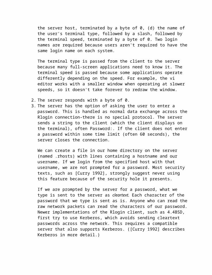
doesn't interpret the return values from the NFS procedures. It normally prints OK and the number of bytes of data in the reply.

Statelessness

One of the features of NFS (critics of NFS would call this a wart, not a feature) is that the NFS server is stateless. "The server does not keep track of which clients are accessing which files. Notice in the list of NFS procedures shown earlier that there is not an open procedure or a close procedure. The LOOKUP procedure is similar to an open, but the server never knows if the client is really going to reference the file after the client does a LOOKUP.

The reason for a stateless design is to simplify the crash recovery of the server after it crashes and reboots.

Example: Server Crash

In the following example we are reading a file from an NFS server when the server crashes and reboots. This shows how the stateless server approach lets the client "not know" that the server crashes. Other than a time pause while the server crashes and reboots, the client is unaware of the problem, and the client application is not affected.

On the client sun we start a cat of a long file (/usr/share/lib/termcap on the NFS server svr4), disconnect the Ethernet cable during the transfer, shut down and reboot the server, then reconnect the cable. The client was configured to read 1024 bytes per NFS read. Figure 29.9 shows the tcpdump output.

1 0.0 sun.7ade > svr4.nfs: 104 getattr 2 0.007653 ( 0.0077) svr4.nfs > sun.7ade: reply ok 96 3 0.009041 ( 0.0014) sun.7adf > svr4.nfs: 116 lookup "share" 4 0.017237 ( 0.0082) svr4.nfs > sun.7adf: reply ok 128 5 0.018518 ( 0.0013) sun.7ae0 > svr4.nfs: 112 lookup "lib" 6 0.026802 ( 0.0083) svr4.nfs > sun.7ae0: reply ok 128 7 0.028096 ( 0.0013) sun.7ael > svr4.nfs: 116 lookup "termcap" 8 0.036434 ( 0.0083) svr4.nfs > sun.7ael: reply ok 128 9 0.038060 ( 0.0016) sun.7ae2 > svr4.nfs: 104 getattr 10 0.045821 ( 0.0078) svr4.nfs > sun.7ae2: reply ok 96 11 0.050984 ( 0.0052) sun.7ae3 > svr4.nfs: 116 read 1024 bytes @ 0 12 0.084995 ( 0.0340) svr4.nfs > sun.7ae3: reply ok 1124

reading continues 128 3.430313 ( 0.0013) sun.7b22 > svr4.nfs: 116 read 1024 bytes @ 64512 129 3.441828 ( 0.0115) svr4.nfs > sun.7b22: reply ok 1124 130 4.125031 ( 0.6832) sun.7b23 > svr4.nfs: 116 read 1024 bytes @ 65536 131 4.868593 ( 0.7436) sun.7b24 > svr4.nfs: 116 read 1024 bytes @ 73728

132 4.993021 ( 0.1244) sun.7b23 > svr4.nfs: 116 read 1024 bytes @ 65536 133 5.732217 ( 0.7392) sun.7b24 > svr4.nfs: 116 read 1024 bytes @ 73728 134 6.732084 ( 0.9999) sun.7b23 > svr4.nfs: 116 read 1024 bytes @ 65536 135 7.472098 ( 0.7400) sun.7b24 > svr4.nfs: 116 read 1024 bytes @ 73728 136 10.211964 ( 2.7399) sun.7b23 > svr4.nfs: 116 read 1024 bytes @ 65536 137 10.951960 ( 0.7400) sun.7b24 > svr4.nfs: 116 read 1024 bytes @ 73728 138 17.171767 ( 6.2198) sun.7b23 > svr4.nfs: 116 read 1024 bytes @ 65536 139 17.911762 ( 0.7400) sun.7b24 > svr4.nfs: 116 read 1024 bytes @ 73728 140 31.092136 (13.1804) sun.7b23 > svr4.nfs: 116 read 1024 bytes @ 65536 141 31.831432 ( 0.7393) sun.7b24 > svr4.nfs: 116 read 1024 bytes @ 73728 142 51.090854 (19.2594) sun.7b23 > svr4.nfs: 116 read 1024 bytes @ 65536 143 51.830939 ( 0.7401) sun.7b24 > svr4.nfs: 116 read 1024 bytes @ 73728 144 71.090305 (19.2594) sun.7b23 > svr4.nfs: 116 read 1024 bytes @ 65536 145 71.830155 ( 0.7398) sun.7b24 > svr4.nfs: 116 read 1024 bytes @ 73728

retransmissions continue 167 291.824285 ( 0.7400) sun.7b24 > svr4.nfs: 116 read 1024 bytes @ 73728 168 311.083676 (19.2594) sun.7b23 > svr4.nfs: 116 read 1024 bytes @ 65536

server reboots 169 311.149476 ( 0.0658) arp who-has sun tell svr4170 311.150004 ( 0.0005) arp reply sun is-at 8:0:20:3:f6:42 171 311.154852 ( 0.0048) svr4.nfs > sun.7b23: reply ok 1124 172 311.156671 ( 0.0018) sun.7b25 > svr4.nfs: 116 read 1024 bytes @ 66560 173 311.168926 ( 0.0123) svr4.nfs > sun.7b25: reply ok 1124

reading continues Figure 29.9 Client reading a file when an NFS server crashes and reboots.

Lines 1-10 correspond to the client opening the file. The operations are similar to those shown in Figure 29.7. In line II we see the first READ of the file, with 1024 bytes of data returned in line 12. This continues (a READ of 1024 followed by a reply of OK) through line 129.

In lines 130 and 131 we see two requests that time out and are retransmitted in lines 132 and 133. The first question is why are there two read requests, one starting at offset 65536 and the other starting at 73728? The client kernel has detected that the client application is performing sequential reads, and is trying to prefetch data blocks. (Most Unix kernels do this read-ahead.) The client kernel is also running multiple NFS block I/O daemons (biod processes) that try to generate multiple RPC requests on behalf of clients. One daemon is reading 8192 bytes starting at 65536 (in 1024-byte chunks) and the other is performing the read-ahead of 8192 bytes starting at 73728.

Client retransmissions occur in lines 130-168. In line 169 we see the server has rebooted, and it sends an ARP request before it can reply to the client's NFS request in line 168. The response to line 168 is sent in line 171. The client READ requests continue.

The client application never knows that the server crashes and reboots, and except for the 5-minute pause between lines 129 and 171, this server crash is transparent to the client.

To examine the timeout and retransmission interval in this example, realize that there are two client daemons with their own timeouts. The intervals for the first daemon (reading at offset 65536), rounded to two decimal points, are: 0.68, 0.87, 1.74, 3.48, 6.96, 13.92, 20.0, 20.0, 20.0, and so on. The intervals for the second daemon (reading at offset 73728) are the same (to two decimal points). It appears that these NFS clients are using a timeout that is a multiple of 0.875 seconds with an upper bound of 20 seconds. After each timeout the retransmission interval is doubled: 0.875, 1.75,3.5, 7.0, and 14.0.

How long does the client retransmit? The client has two options that affect this. First, if the server filesystem is mounted hard, the client retransmits forever, but if the server filesystem is mounted soft, the client gives up after a fixed number of retransmissions. Also, with a hard mount the client has an option of whether to let the user interrupt the infinite retransmissions or not. If the client host specifies interruptibility when it mounts the server's filesystem, if we don't want to wait 5 minutes for the server to reboot after it crashes, we can type our interrupt key to abort the client application.

Idempotent Procedures

An RPC procedure is called idempotent if it can be executed more than once by the server and still return the same result. For example, the NFS read procedure is idempotent. As we saw in Figure 29.9, the client just reissues a given READ call until it gets a response. In our example the reason for the retransmission was that the server had crashed. If the server hasn't crashed, and the RPC reply message is lost (since UDP is unreliable), the client just retransmits and the server performs the same READ again. The same portion of the same file is read again and sent back to the client.

This works because each READ request specifies the starting offset of the read. If there were an NFS procedure asking the server to read the next N bytes of a file, this wouldn't work. Unless the server is made stateful (as opposed to stateless), if a reply is lost and the client reissues the READ for the next N bytes, the result is different. This is why the NFS READ and WRITE procedures have the client specify the starting offset. The client maintains the state (the current offset of each file), not the server.

Unfortunately, not all filesystem operations are idempotent. For example, consider the following steps: the client NFS issues the REMOVE request to delete a file; the server NFS deletes the file and responds OK; the server's response is lost; the client NFS times out and retransmits the request; the server NFS can't find the file and responds with an error; the client application receives an error saying the file doesn't exist. This error return to the client application is wrong-the file did exist and was deleted.

The NFS operations that are idempotent are: GETATTR, STATES, LOOKUP, READ, WRITE, READLINK, and READDIR. The procedures that are not idempotent are: CREATE, REMOVE,

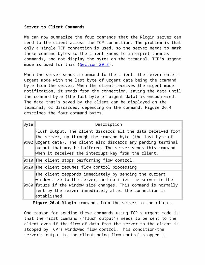
RENAME, LINK, SYMLINK, MKDIR, and RMDIR. SETATTR is normally idempotent, unless it's being used to truncate a file.

Since lost responses can always happen with UDP, NFS servers need a way to handle the nonidempotent operations. Most servers implement a recent-reply cache in which they store recent replies for the nonidempotent operations. Each time the server receives a request, it first checks this cache, and if a match is found, returns the previous reply instead of calling the NFS procedure again. [Juszczak 1989] provides details on this type of cache.

This concept of idempotent server procedures applies to any UDP-based application, not just NFS. The DNS, for example, provides an idempotent service. A DNS server can execute a resolver's request any number of times with no ill effects (other than wasted network resources).

TCP/IP Applications

30.1 Introduction

In this chapter we describe additional TCP/IP applications that many implementations support. Some are simple and easy to cover completely (Finger and Whois), while another is complex (the X Window System). We provide only a brief overview of this complex application, focusing on its use of the TCP/IP protocols.

Additionally we provide an overview of some Internet resource discovery tools. These are tools to help us navigate our way around the Internet, searching for items whose location and exact name we don't know.

30.2 Finger Protocol

The Finger protocol returns information on one or more users on a specified host. It's commonly used to see if someone is currently logged on, or to figure out someone's login name, to send them mail. RFC 1288 [Zimmerman 1991] specifies the protocol.

Many sites do not run a Finger server for two reasons. First, a programming error in an earlier version of the server was one of the entry points used by the infamous Internet worm of 1988. (RFC 1135 [Reynolds 1989] and [Curry 1992] describe the worm in more detail.) Second, the Finger protocol can reveal detailed information on users (login names, phone numbers, when they last logged in, etc.) that many administrators consider private. Section 3 of RFC 1288 details the security aspects of this service.

From a protocol perspective, the Finger server has a well-known port of 79. The client does an active open to this port and sends a one-line query The server processes the query, sends back the output, and closes the connection. The query and response are NVT ASCII, similar to what we saw with FTP and SMTP.

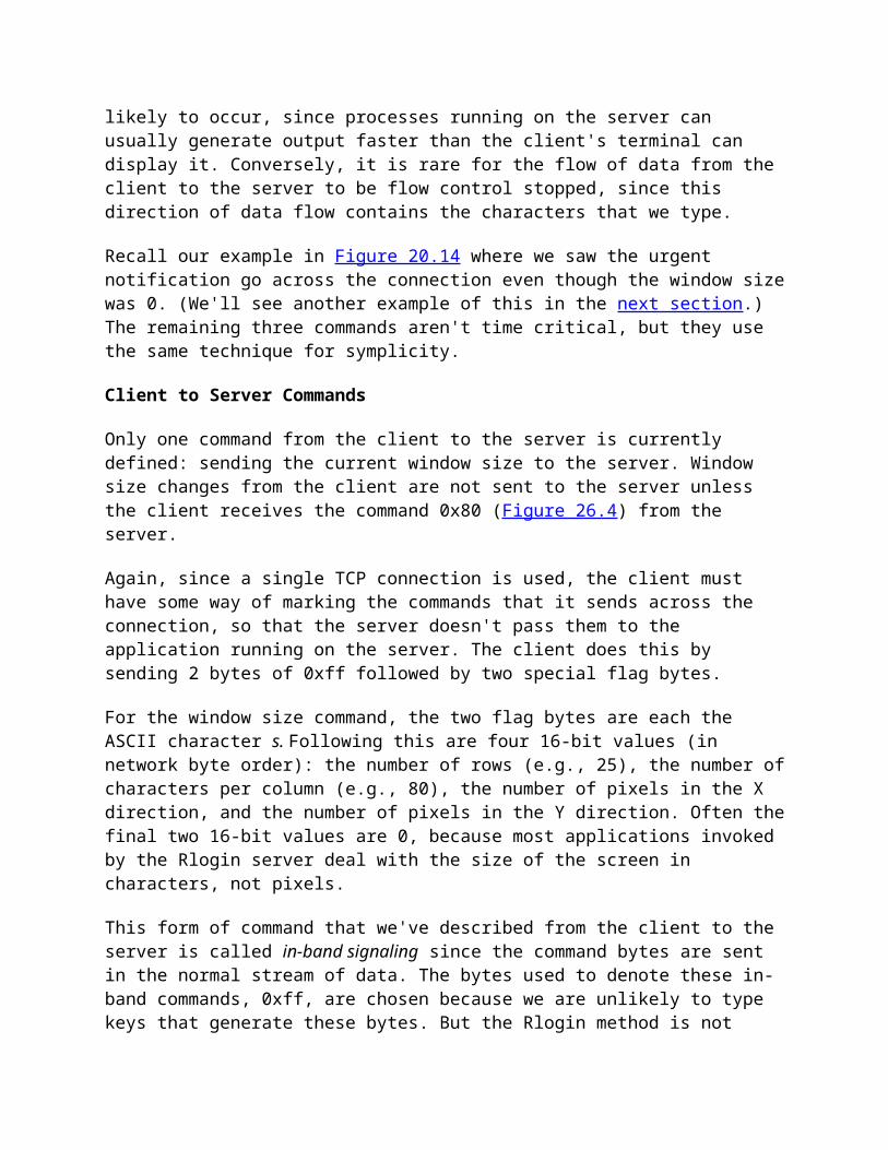
While most Unix users access the Finger server using the finger(l) client, we'll start by using the Telnet client to connect directly to the server and see the one-line commands issued by the client. If the client query is an empty line (which in NVT ASCII is transmitted as a CR followed by an LF), it is a request for information on all online users.

sun % telnet slip finger Trying 140.252.13.65 ... first three lines are output by Telnet client Connected to slip.Escape character is '^]' .

here we type RETURN as the Finger client command Login Name Tty Idle Login Time Office Office Phone rstevens Richard Stevens *co 45 Jul 31 09:13 rstevens Richard Stevens *c2 45 Aug 5 09:41 Connection closed by foreign host. output by Telnet client

The blank output fields for the office and office phone are taken from optional fields in the user's password file entry (which aren't present in this example).

The server must be the end that does the active close, since a variable amount of information is returned by the server, and the reception of the end-of-file by the client is how the client knows when the output is complete.

When the client request consists of a usemame, the server responds with information only about that user. Here's another example, with the Telnet client output removed:

sun % telnet vangogh.cs.berkeley.edu finger rstevens this is the client request we type Login: rstevens Name: Richard Stevens Directory: /a/guest/rstevens Shell: /bin/csh Last login Thu Aug 5 09:55 (PDT) on ttyq2 from sun.tuc.noao.edu Mail forwarded to: rstevens@noao.edu No Plan.

When a system has the Finger service completely disabled, the client's active open will receive an RST from the server, since no process has a passive open on port 79:

sun % finger @svr4[svr4.tuc.noao.edu] connect: Connection refused

Some sites provide a server on port 79, but it just outputs information to the client, and doesn't honor any client requests:

sun % finger @att.com [att.com] this line output by Finger client; remainder from

server ---------------------------------------------------------------------------------- There are no user accounts on the AT&T Internet gateway, To send email to an AT&T employee, send email to their name separated by periods at att.com. If the employee has an email address registered in the employee database, they will receive email - otherwise, you'll receive a non-delivery notice. For example: John.Q.Public@att.com sun % finger clinton@whitehouse.gov [whitehouse.gov]Finger service for arbitrary addresses on whitehouse.gov is not supported. If you wish to send electronic mail, valid addresses are "PRESIDENT@WHITEHOUSE.GOV", and "VICE-PRESIDENT@WHITEHOUSE.GOV"

Another possibility is for an organization to implement a firewall gateway: a router between the organization and the Internet that filters out (i.e., discards) certain IP datagrams. ([Cheswick and Bellovin 1994] discuss firewall gateways in detail.) The firewall gateway can be configured to discard incoming datagrams that are TCP segments for port 79. In this case the Finger client times out after about 75 seconds.

There are additional options for the Finger server, and for the Unix finger client. Refer to RFC 1288 and the finger(l) manual page for the details.

RFC 1288 states that vending machines with TCP/IP connections that provide a Finger server should reply to a client request consisting of a blank line with a list of all items currently available. They should reply to a client request consisting of a name with a count or list of available items for that product.

30.3 Whois Protocol

The Whois protocol is another information service. Although any site can provide a Whois server, the one at the InterNIC, rs.internic.net, is most commonly used. This server maintains information about all registered DNS domains and many system administrators responsible for systems connected to the Internet. (Another server is provided at nic.ddn.mil, but contains information only about the MILNET.) Unfortunately the information can be out of data or incomplete. RFC 954 [Harrenstien, Stahl, and Feinler 1985] documents the Whois service.

From a protocol perspective, the Whois server has a well-known TCP port of 43. It accepts connection requests from clients, and the client sends a one-line query to the server. The server responds with whatever information is available and then closes the connection. The requests and replies are transmitted using NVT ASCII. This is almost identical to the Finger server, although the requests and replies contain different information.

The common Unix client is the whois(1) program, although we can use Telnet and type in the commands ourself. The starting place is to send a request consisting of just a question mark, which returns more detailed information on the supported client requests.

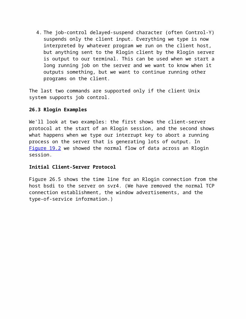
When the NIC moved to the InterNIC in 1993, the site for the Whois server moved from nic.ddn.mil to rs.internic.net. Many vendors still ship versions of the whois client with the name nic.ddn.mil built in. You may need to specify the command-line argument -h rs.internic.net to contact the correct server.

Alternately, we can Telnet to rs.internic.net and login as whois.

We'll use the Whois server to track down the author. (We've removed the extraneous Telnet client output.) Our first request is for all names that match "stevens."

sun % telnet rs.internic.net whois stevens this is the client command we type

information on 25 other "stevens" that we omit

Stevens, W. Richard (WRS28) stevens@kohala.com +1 602 297 9416 The InterNIC Registration Services Host ONLY contains Internet Information (Networks, ASN's, Domains, and POC's). Please use the whois server at nic.ddn.mil for MILNET Information.

The three uppercase letters followed by a number in parentheses after the name, (WRS28), are the person's NIC handle. The next query contains an exclamation point and a NIC handle, to fetch more information about this person.

sun % telnet rs.internic.net whois !wrs28 client request that we type Stevens, W. Richard (WRS28) stevens@kohala.com Kohala Software 1202 E. Paseo del Zorro Tucson, AZ 85718 +1 602 297 9416 Record last updated on 11-Jan-91.

Lots of additional information about Internet variables can also be queried. For example, the request net 140.252 returns information about the class B address 140.252.

White Pages

Using the VRFY command of SMTP, along with the Finger protocol and the Whois protocol to locate users on the Internet is similar to using the white pages of a telephone book to find someone's phone number. At the present time ad hoc tools such as these are all that's widely available, but research is under way to improve this type of service.

[Schwartz and Tsirigotis 1991] contains additional information on various white pages services being tried on the Internet. The particular tool, called Netfind, can be accessed by using Telnet to either bruno.cs.colorado.edu or ds.internic.net and logging in as netfind.

RFC 1309 [Weider, Reynolds, and Heker 1992] provides an overview of the OSI directory service, called X.500, and compares and contrasts it with current Internet techniques (Finger and Whois).

30.4 Archie, WAIS, Gopher, Veronica, and WWW

The tools that we described in the previous two sections-Finger, Whois, and a white pages service-are for locating information on people. Other tools exist to locate files and documents, and this section gives an overview of these tools. We only provide an overview, because examining the details of each tool is beyond the scope of this book. Methods are given for accessing these tools across the Internet, and you are encouraged to do so, to find which tool can help you. Additional tools are continually being developed. [Obraczka, Danzig, and Li 1993] provide an overview of resource discovery services on the Internet.

Archie

Many of the resources used in this text were obtained using anonymous FTP. The problem is finding which FTP site has the program we want. Sometimes we don't even know the exact filename, but we know some keywords that probably appear in the filename.

Archie provides a directory of thousands of FTP servers across the Internet. We can access this directory by logging into an Archie server and searching for files whose name contains a specified regular expression. The output is a list of servers with matching filenames. We then use anonymous FTP to that site to fetch the file.

There are many Archie servers across the world. One starting point is to use Telnet to ds.internic.net, login as archie, and execute the command servers. This provides a list of all the Archie servers, and their location.

WAIS: Wide Area Information Servers

Archie helps us locate filenames that contain keywords, but sometimes we're looking for a file or database that contains a keyword. That is, we want to search for a file that contains a keyword, not a filename containing a keyword.

WAIS knows about hundreds of databases that contain information on both computer-related topics and other general topics. To use WAIS we select the databases to search and specify the keywords. To try WAIS Telnet to quake.think.com and login as wais.

Gopher

Gopher is a menu-driven front end to other Internet resource services, such as Archie, WAIS, and anonymous FTP Gopher is one of the easiest to use, since its user interface is the same, regardless of which resource service it's using.

To use Gopher, Telnet into is.internic.net and login as gopher.

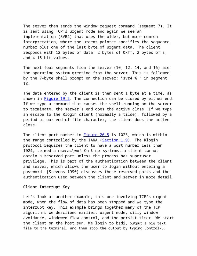
Veronica: Very Easy Rodent-Oriented Netwide Index to Computerized Archives

Just as Archie is an index of anonymous FTP servers. Veronica is an index of titles of Gopher items. A Veronica search typically searches hundreds of Gopher servers.

To access Veronica we must go through a Gopher client. Select the Gopher menu item "Beyond InterNIC: Virtual Treasures of the Internet" and then select Veronica from the next menu.

WWW: World Wide Web

World Wide Web lets us browse a large, worldwide set of services and documents using a tool called hypertext. As information is displayed, certain keywords are highlighted, and we can select more information on those keywords. To access WWW, Telnet to info.cern.ch.

30.5 X Window System

The X Window System, or just X, is a client-server application that lets multiple clients (applications) use the bit-mapped display managed by a server. "The server is the software that manages a display, keyboard, and mouse. The client is an application program that runs on either the same host as the server or on a different host. In the latter case the common form of communication between the client and server is TCP, although other protocols such as DECNET can be used. In some instances the server is a dedicated piece of hardware (an X terminal) that communicates with clients on other hosts. In another instance, a stand-alone workstation, the client and server are on the same host and communicate using interprocess communication on that host, without any network involvement at all. Between these two extremes is a workstation that supports clients on the same host and clients on other hosts.

X requires a reliable, bidirectional stream protocol, such as TCP. (X was not designed for an unreliable protocol such as UDP.) The communication between the client and server consists of 8-bit bytes exchanged across this connection. [Nye 1992] gives the format of the more than 150 messages exchanged between the client and server across their TCP connection.

On a Unix system, when the X client and X server are on the same host, the Unix domain protocols are normally used instead of TCP, because there is less protocol processing than if TCP were used. The Unix domain protocols are a form of interprocess communication that can be used between clients and servers on the same host. Recall in Figure 2.4 that when TCP is used for communication between two processes on the same host, the loopback of this data takes place below the IP layer, implying that all the TCP and IP processing takes place.

Figure 30.1 shows one possible scenario with three clients using one display. One client is on the same host as the server, using the Unix domain protocols. The other two clients are on different hosts, using TCP. One client is normally a window manager that has authority

for the layout of windows on the display. The window manager allows us to move windows around the screen, or change their size, for example.

Figure 30.1 Three X clients using one display.

On first glance the terms client and server appear backward. With applications such as Telnet and FTP we think of the client as the interactive user at the keyboard and display. But with X, the keyboard and display belong to the server. Think of the server as the end providing the service. The service provided by X is access to a window, keyboard, and mouse. With Telnet the service is logging in to the remote host. With FTP the service is the filesystem on the server.

The X server is normally started when the X terminal or workstation is bootstrapped. The server creates a TCP end point and does a passive open on port 6000 + n, where n is the display number (normally 0). Most Unix servers also create a Unix domain socket with the name /tmp/.X11-unix/Xn, where n is again the display number.

When a client is started on another host, it creates a TCP end point and performs an active open to port 6000 + n on the server. Each client gets its own TCP connection to the server. It is the server's responsibility to multiplex all the clients. From this point on the client sends requests to the server across the TCP connection (e.g., create a window), the server sends back replies, and the server also sends events to the client (mouse button pushed, keyboard key pressed, window exposed, window resized, etc.).

Figure 30.2 is a redo of Figure 30.1, emphasizing that the clients communicate with the X server process, which in turn manages the windows on the display. Not shown here is that the X server also manages the keyboard and mouse.

Figure 30.2 Three clients using one display.

This design, where a single server handles multiple clients, differs from the normal TCP concurrent server design that we described in Section 18.11. The FTP and Telnet servers, for example, spawn a new process each time a new TCP connection request arrives, so each client communicates with a different server process. With X, however, all clients, running on the same host or on a different host, communicate with a single server.

Lots of data can be exchanged across the TCP connection between an X client and its server. The amount depends on the specific application design. For example, if we run the Xclock client, which displays the current time and date on the client in a window on the server, specifying an update of once a second, an X message is sent across the TCP connection from the client to the server once a second. If we run the X terminal emulator, Xterm, each keystroke we type becomes a 32-byte X message (72 bytes with the standard IP and TCP headers), with a larger X message in the reverse direction with the character echo. [Droms and Dyksen 1990] measure the TCP traffic between various X clients and one particular server.

Xscope Program

A handy program for examining what's exchanged between an X client and its server is Xscope. It's provided with most X window implementations. It sits between a client and server, passing everything in both directions, and also deciphering all the client requests and server replies. Figure 30.3 shows the setup.

Figure 30.3 Using xscope to monitor an X connection.

We first start the xscope process on the same host as the server, but xscope listens for TCP connection requests on port 6001, not 6000. We then start a client on another host and specify display number 1, not 0, so the client connects to xscope, not directly to the server. When the connection request from the client arrives, xscope creates a TCP connection to the real server at port 6000, and copies everything between the client and server, and produces a readable description of the requests and replies.

We'll start xscope on our host sun and then run the xclock client on the host svr4.

svr4 % DISPLAY=sun:l xclock -digital -update 5

This displays the time and date in the digital format

Thu Sep 9 10:32:55 1993

in a window on the host sun. We specify an update time of once every 5 seconds.

We specify the -q option for xscope to produce minimal output. Various levels of verbosity are available, to see all the fields in each message. The following output shows the first three requests and replies.

sun % xscope -q0.00: Client -> 12 bytes0.02: 152 bytes <-- X11 Server 0.03: Client -> 48 bytes............REQUEST: CreateGC............REQUEST: GetProperty0.20: 396 bytes <-- X11 Server

..............REPLY: GetProperty 0.30: Client -> 8 bytes0.38: Client -> 20 bytes............REQUEST: InternAtom0.43: 32 bytes <-- XII Server

..............REPLY: InternAtom

The first client message at time 0.00 and the server's response at time 0.02 are the standard connection setup between the client and server. The client identifies its byte ordering and the version of the server that it expects. The server responds with various information about itself.

The next message at time 0.03 contains two client requests. The first request creates a graphics context in the server in which the client will draw. The second gets a property from the server (the RESOURCEJVIANAGER property). Properties provide for communication between clients, often between an application and the window manager. The server's 396-byte reply at time 0.20 contains this property.

The next two messages from the client at times 0.30 and 0.38 form a single request to return an atom. (Each property has a unique integer ID called an atom.) The server replies at time 0.43 with the atom.

It is impossible to delve farther into this example without providing lots of details about the X window system, which isn't the purpose of this section. In this example a total of 12 segments comprising 1668 bytes is sent by the client and a total of 10 segments comprising 1120 bytes is sent by the server, before the window is displayed. The elapsed time was 3.17 seconds. From this point the client sent a small request every 5 seconds, averaging 44 bytes, with an update to the window. This continued until the client was terminated.

LBX: Low Bandwidth X

The encoding used by the X protocol is optimized for LANs, where the time spent encoding and decoding the data is more important than minimizing the amount of data transmitted. While this is OK for an Ethernet, it becomes a problem for slow serial lines, such as SLIP and PPP links (Sections 2.4 and 2.6).

Work is progressing to define a standard called Low Bandwidth X (LBX) that uses the following techniques to reduce the amount of network traffic: caching, sending differences from previous packets, and compression. Specifications should appear early in 1994 with a sample implementation in the X window system Release 6.