T.C ATILIM UNIVERSITY

MODES ADVANCED SYSTEM SIMULATION

MODES 650

A COMPREHENSIVE REVIEW OF METHODS FOR SIMULATION OUTPUT ANALYSIS

Christos AlexopoulosSchool of Industrial and Systems Engineering

Georgia Institute of TechnologyAtlanta, Georgia 30332–0205, U.S.A.

represented by:

Adel Agila

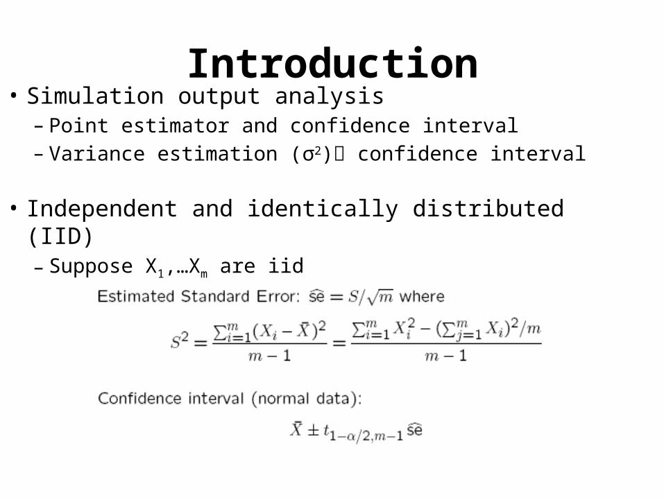
Introduction• Simulation output analysis – Point estimator and confidence interval– Variance estimation (σ2) confidence interval

• Independent and identically distributed (IID)– Suppose X1,…Xm are iid

The Methods

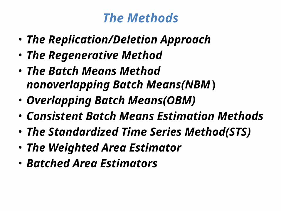
• The Replication/Deletion Approach• The Regenerative Method• The Batch Means Method

nonoverlapping Batch Means(NBM)• Overlapping Batch Means(OBM)• Consistent Batch Means Estimation Methods• The Standardized Time Series Method(STS)• The Weighted Area Estimator• Batched Area Estimators

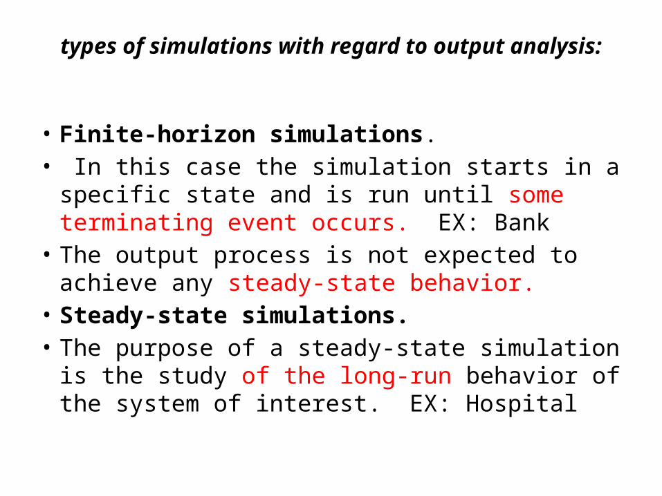
types of simulations with regard to output analysis:

• Finite-horizon simulations.• In this case the simulation starts in a specific state

and is run until some terminating event occurs. EX: Bank

• The output process is not expected to achieve any steady-state behavior.

• Steady-state simulations. • The purpose of a steady-state simulation is the

study of the long-run behavior of the system of interest. EX: Hospital

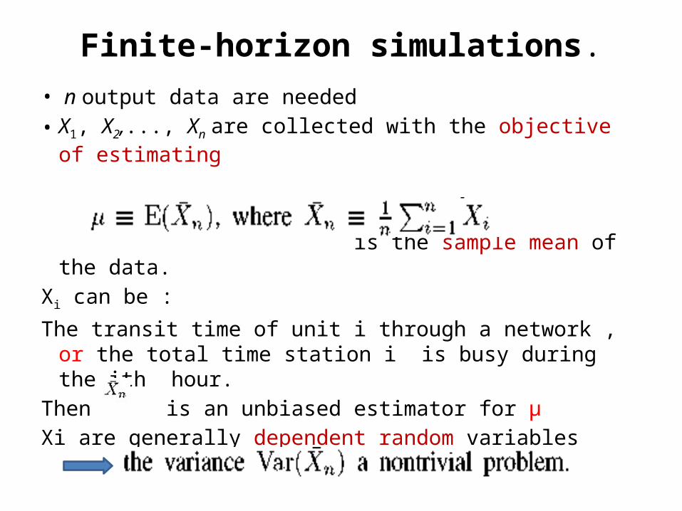
Finite-horizon simulations.• n output data are needed • X1, X2,..., Xn are collected with the objective of

estimating

is the sample mean of the data.Xi can be :

The transit time of unit i through a network , or the total time station i is busy during the ith hour.

Then is an unbiased estimator for μ Xi are generally dependent random variables

Finite-horizon simulations.

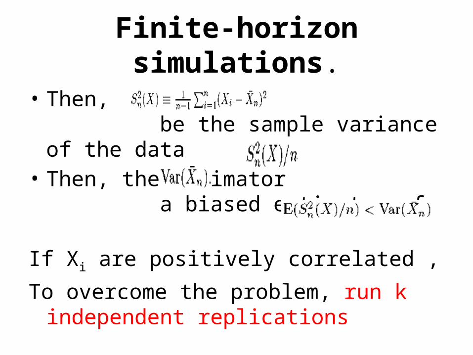
• Then, let be the sample variance of the data

• Then, the estimator a biased estimator of

If Xi are positively correlated ,

To overcome the problem, run k independent replications

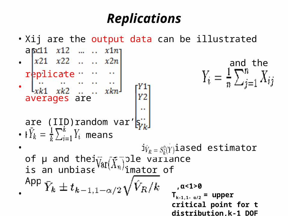
Replications

• Xij are the output data can be illustrated as:• and the replicate • averages are are (IID)random var’s• Here their means• is unbiased estimator of μ and

their sample variance is an unbiased estimator of Approximate 1-α cI for u

• 0<α<1 ,Tk-1,1- α/2 = upper critical point for t distribution,k-1 DOF

STEADY-STATE ANALYSIS

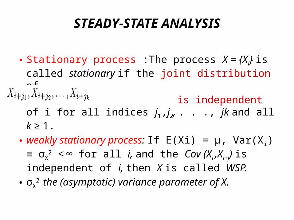
• Stationary process :The process X = {Xi} is called stationary if the joint distribution of

is independent of i for all indices j1,j2, . . ., jk and all k ≥ 1.

• weakly stationary process: If E(Xi) = µ, Var(Xi) ≡ σX

2 < ∞ for all i, and the Cov (Xi ,Xi+j) is independent of i, then X is called WSP.

• σX2 the (asymptotic) variance parameter of X.

Stationary Process

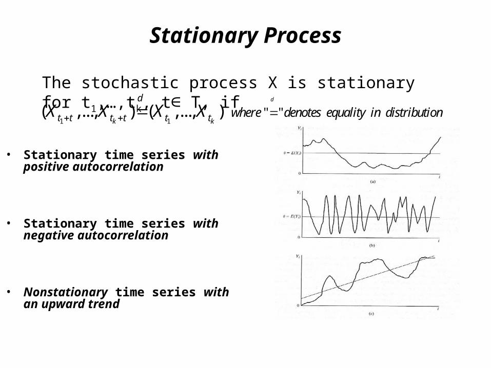
• Stationary time series with positive autocorrelation

• Stationary time series with negative autocorrelation

• Nonstationary time series with an upward trend

The stochastic process X is stationary for t1,…,tk, t T, if∈

1 1" "( ,..., ) ( ,..., )

d

k k

d

t t t t t t where denotes equality in distributionX X X X

Stationary Process

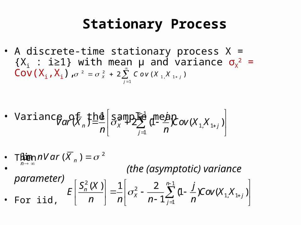
• A discrete-time stationary process X = {Xi : i≥1} with mean µ and variance σX

2 = Cov(Xi,Xi),

• Variance of the sample mean

• Then• (the (asymptotic) variance parameter)

• For iid,

2 21, 1

1

2 ( )X jj

Cov X X

2lim ( )nnnVar X

2 12

1, 11

( ) 1 2(1 ) ( )

1

nn

X jj

S X jE Cov X X

n n n n

12

1, 11

1( ) 2 (1 ) ( )

n

n X jj

jVar X Cov X X

n n

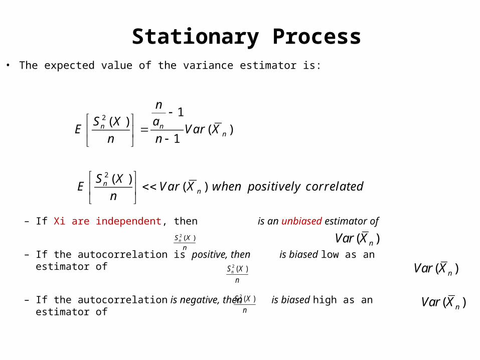
Stationary Process • The expected value of the variance estimator is:

– If Xi are independent, then is an unbiased estimator of

– If the autocorrelation is positive, then is biased low as an estimator of

– If the autocorrelation is negative, then is biased high as an estimator of

2

2

1( )

( )1

( )( )

n nn

nn

nS X a

E Var Xn n

S XE Var X when positively correlated

n

( )nVar X

( )nVar X

( )nVar X2 ( )nS X

n

2 ( )nS X

n

2 ( )nS X

n

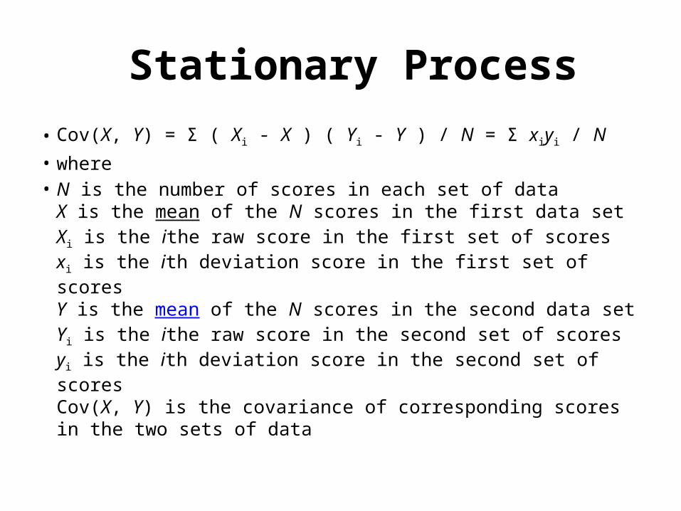
Stationary Process • Cov(X, Y) = Σ ( Xi - X ) ( Yi - Y ) / N = Σ xiyi / N • where• N is the number of scores in each set of data

X is the mean of the N scores in the first data setXi is the ithe raw score in the first set of scoresxi is the ith deviation score in the first set of scoresY is the mean of the N scores in the second data setYi is the ithe raw score in the second set of scoresyi is the ith deviation score in the second set of scoresCov(X, Y) is the covariance of corresponding scores in the two sets of data

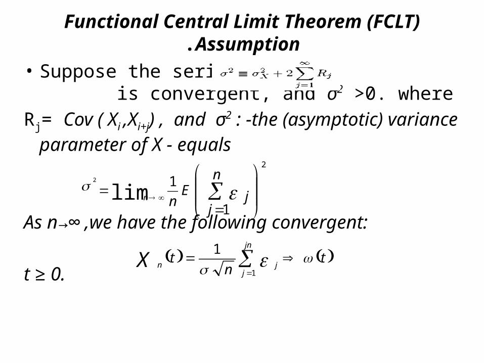
Functional Central Limit Theorem (FCLT) Assumption.

• Suppose the series is convergent, and σ2 >0. where

Rj= Cov ( Xi ,Xi+j) , and σ2 : -the (asymptotic) variance parameter of X - equals

As n→∞ ,we have the following convergent:

t ≥ 0.

tn

tjn

jjnX

1

1

n

jjE

nn

1

12

lim2

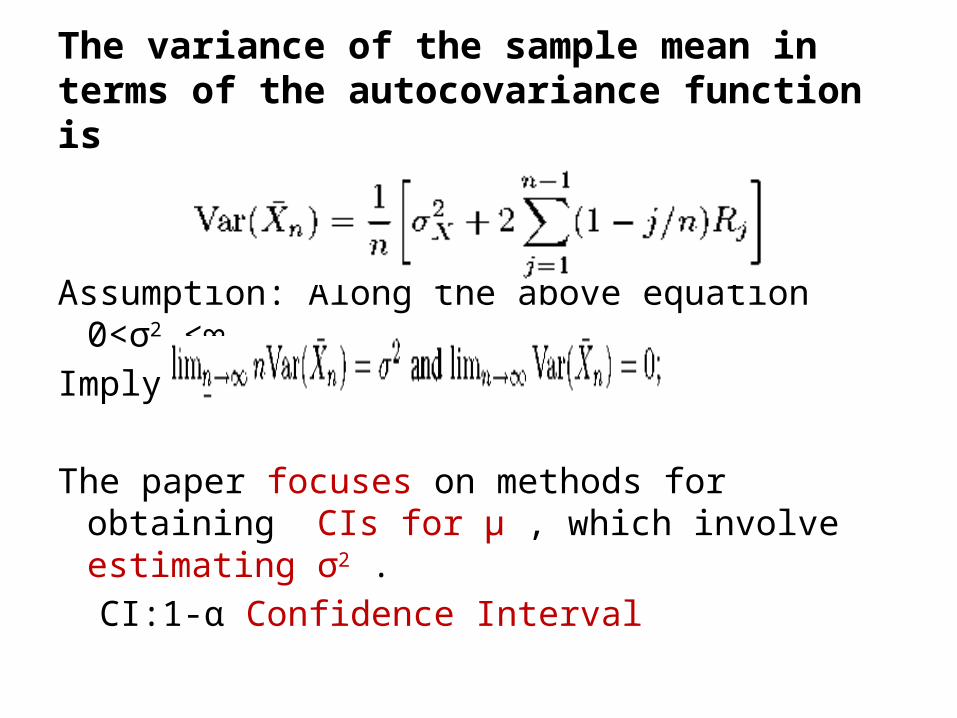
The variance of the sample mean in terms of the autocovariance function is

Assumption: Along the above equation 0<σ2 <∞.Imply

The paper focuses on methods for obtaining CIs for μ , which involve estimating σ2 .

CI:1-α Confidence Interval

The Replication/Deletion Approach

• K independent replications • each of length l +n observations.• Discard the first l observations from each run.• Use the IID sample means • Compute the point estimate • If k is large ,compute the approximate 1-α cI

for μ:Ex: Note

The Replication/Deletion Approach

• For (l ,n, and k)• (a) As l increased for fixed n, the “systematic” error in

each Yi(l , n) due to the initial conditions decreased. • (b) As n increased for fixed l , the systematic and

sampling errors in Yi(l , n) decreased.

• (c) #of replications k cannot effect The Yi(l , n) k.• (d) For fixed n, the CI is valid only if l / lnk → ∞ as k

→ ∞. l increase faster than lnk.• Replication method (more )is expensive

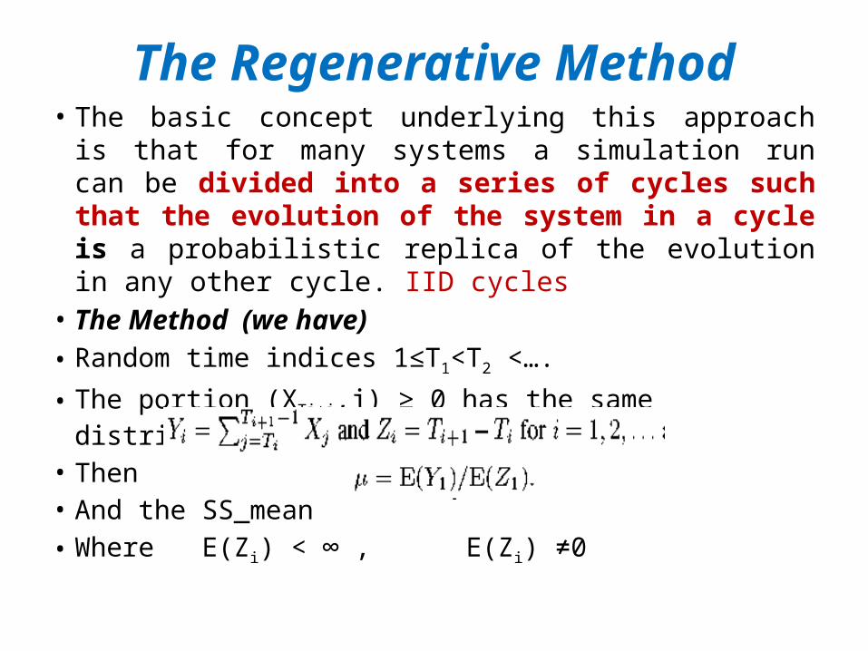
The Regenerative Method• The basic concept underlying this approach is that for

many systems a simulation run can be divided into a series of cycles such that the evolution of the system in a cycle is a probabilistic replica of the evolution in any other cycle. IID cycles

• The Method (we have)• Random time indices 1≤T1<T2 <….

• The portion (XTi+j,j) ≥ 0 has the same distribution for i . • Then • And the SS_mean• Where E(Zi) < ∞ , E(Zi) ≠0

The Regenerative Method

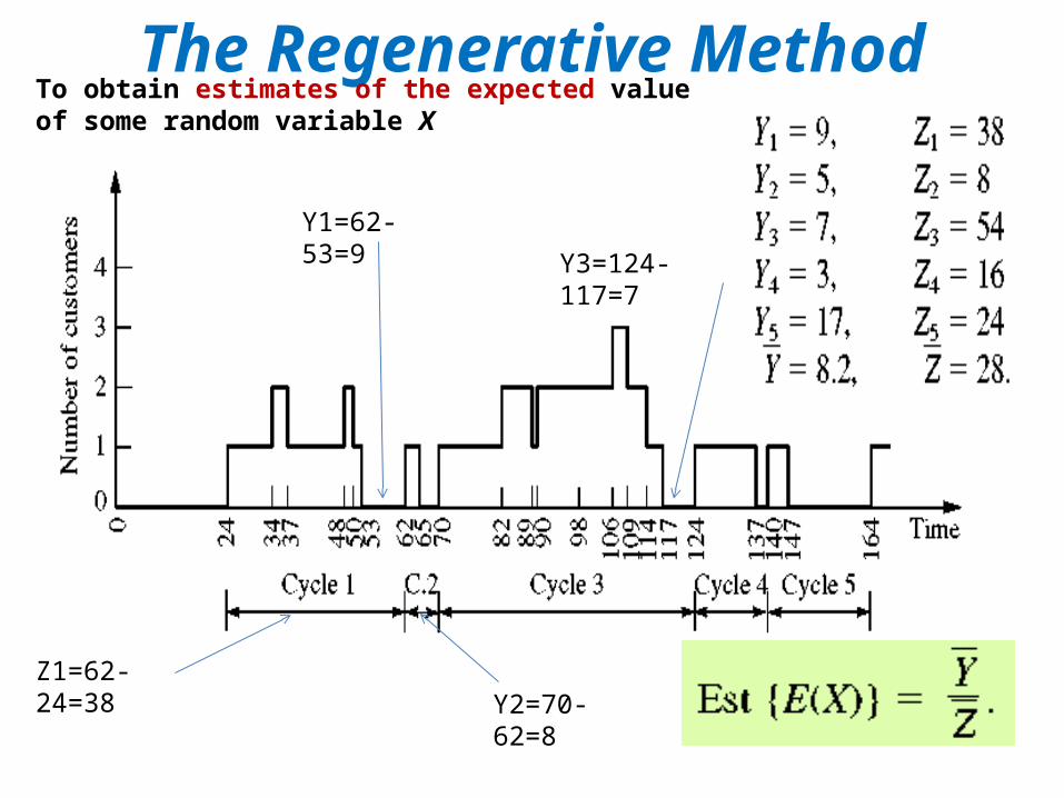
Y1=62-53=9

Y3=124-117=7

Y2=70-62=8Z1=62-24=38

To obtain estimates of the expected value of some random variable X

The Regenerative Method

The Regenerative Method

• Disadvantages• difficult to apply in prac tice because the

majority of simulations have either no regenerative points or very long cycle lengths.

The Batch Means Method nonoverlapping Batch Means(NBM)

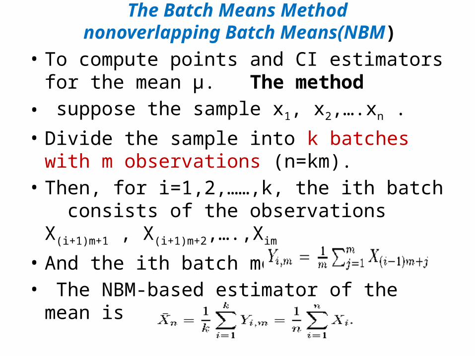
• To compute points and CI estimators for the mean µ. The method

• suppose the sample x1, x2,….xn .• Divide the sample into k batches with m

observations (n=km).• Then, for i=1,2,……,k, the ith batch consists of

the observations X(i+1)m+1 , X(i+1)m+2,….,Xim • And the ith batch mean• The NBM-based estimator of the mean is

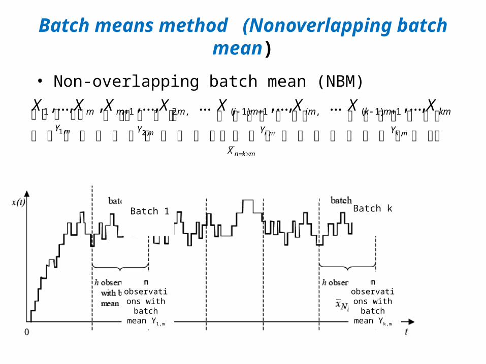
• Non-overlapping batch mean (NBM)

Batch means method (Nonoverlapping batch mean)

m observations

with batch mean Y1,m

Batch 1

m observations

with batch mean Yk,m

Batch k

1, 2, , ,

1 1 2 , ( 1) 1 , ( 1) 1,..., , ,..., ... ,..., ... ,...,

m m i m k m

n k m

m m m i m im k m km

Y Y Y Y

X

X X X X X X X X

Nonoverlapping batch mean (NBM)

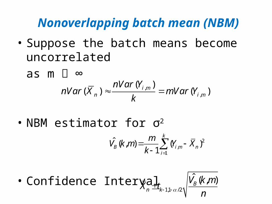
• Suppose the batch means become uncorrelated as m ∞

• NBM estimator for σ2

• Confidence Interval

,,

( )( ) ( )i m

n i m

nVar YnVar X mVar Y

k

2,

1

ˆ ( , ) ( )1

k

B i m ni

mV k m Y X

k

1,1 / 2

ˆ ( , )Bn k

V k mX t

n

Consistent Batch Means Estimation Methods

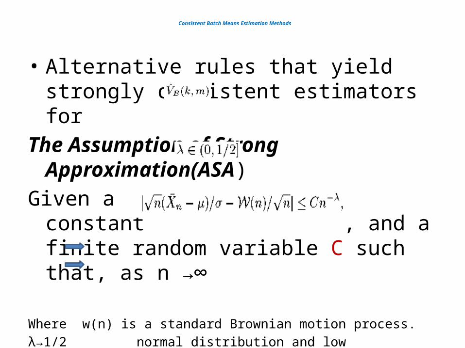
• Alternative rules that yield strongly consistent estimators for

The Assumption of Strong Approximation(ASA)Given a constant , and a finite random

variable C such that, as n →∞

Where w(n) is a standard Brownian motion process. λ→1/2 normal distribution and low correlation among Xi .λ→0 the absence of one of the above .

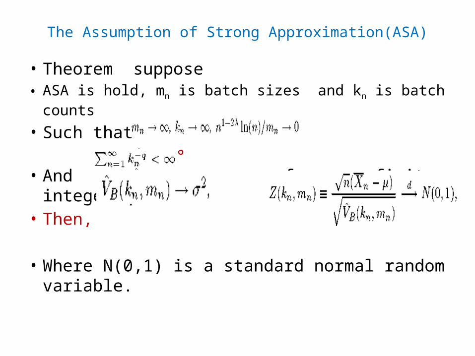
The Assumption of Strong Approximation(ASA)

• Theorem suppose • ASA is hold, mn is batch sizes and kn is batch counts

• Such that , as n →∞ • And for some finite integer q ≥ 1.• Then, and

• Where N(0,1) is a standard normal random variable.

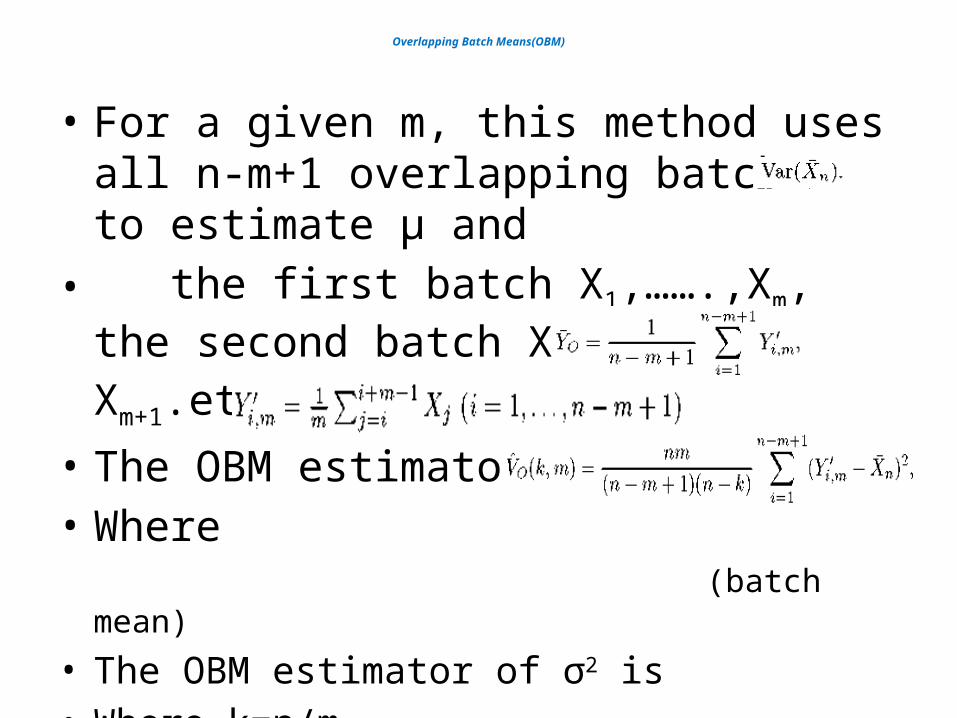
Overlapping Batch Means(OBM)

• For a given m, this method uses all n-m+1 overlapping batches to estimate µ and

• the first batch X1,…….,Xm, the second batch X2,……….., Xm+1.etc

• The OBM estimator of µ is• Where (batch mean)

• The OBM estimator of σ2 is• Where k=n/m.

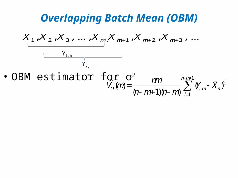
Overlapping Batch Mean (OBM)

• OBM estimator for σ2

1 2 3 , 1 2 3, , , ... , , , , ...m m m mX X X X X X X

Y1,m

Y2,m

12

,1

ˆ ( ) ( )( 1)( )

n m

O i m ni

nmV m Y X

n m n m

NBM vs. OBM

29

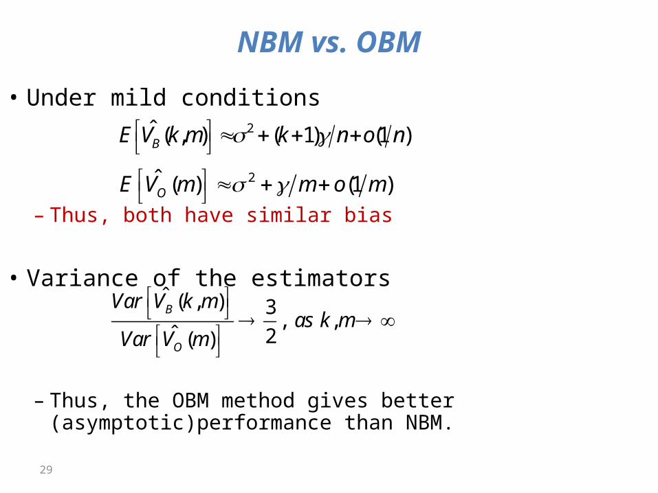
• Under mild conditions

– Thus, both have similar bias

• Variance of the estimators

– Thus, the OBM method gives better (asymptotic)performance than NBM.

2ˆ ( , ) ( 1) (1 )BE V k m k n o n 2ˆ ( ) (1 )OE V m m o m

ˆ ( , ) 3, ,

ˆ 2( )

B

O

Var V k mas k m

Var V m

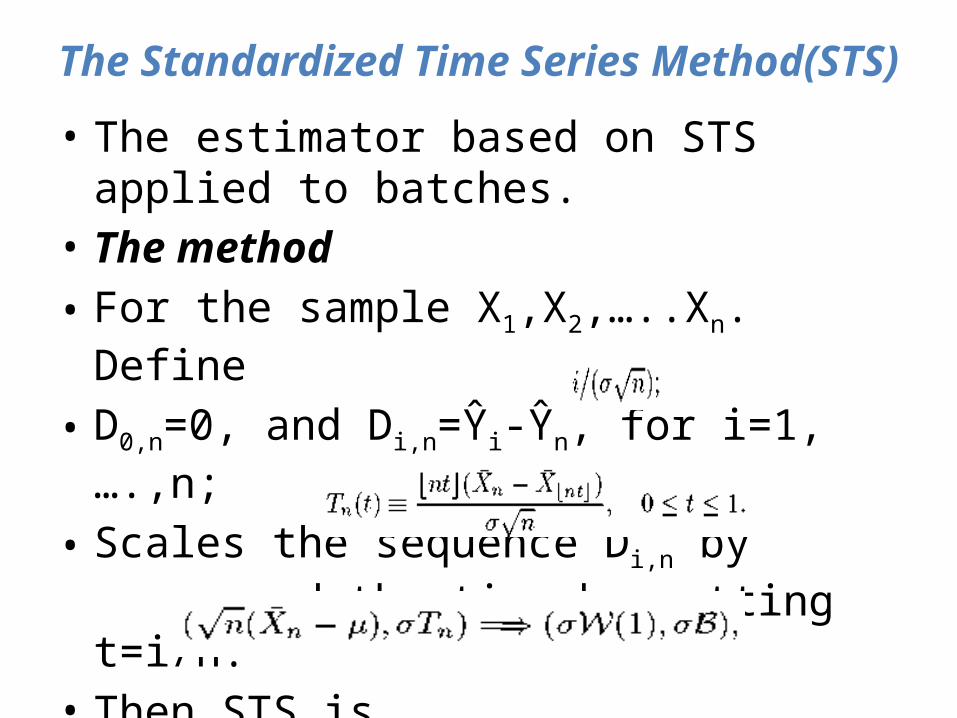
The Standardized Time Series Method(STS)

• The estimator based on STS applied to batches.• The method• For the sample X1,X2,…..Xn. Define

• D0,n=0, and Di,n=Ŷi-Ŷn, for i=1,….,n;

• Scales the sequence Di,n by and the time by setting t=i/n.

• Then STS is• If X satisfies a FCLT, then as n →∞

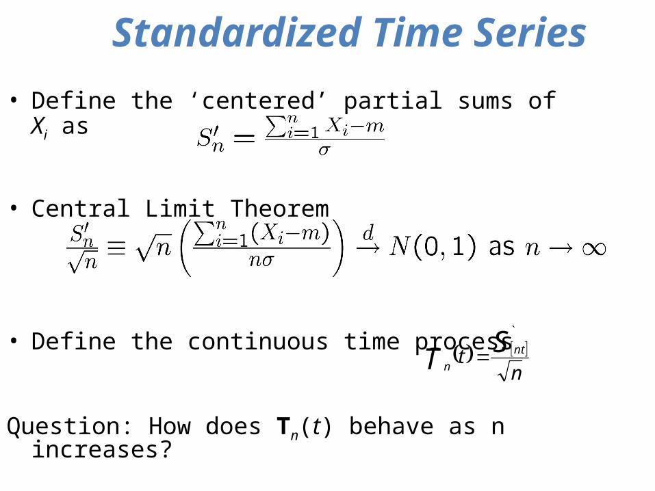
Standardized Time Series • Define the ‘centered’ partial sums of Xi as

• Central Limit Theorem

• Define the continuous time process

Question: How does Tn(t) behave as n increases?

ntS

T nt

n

`

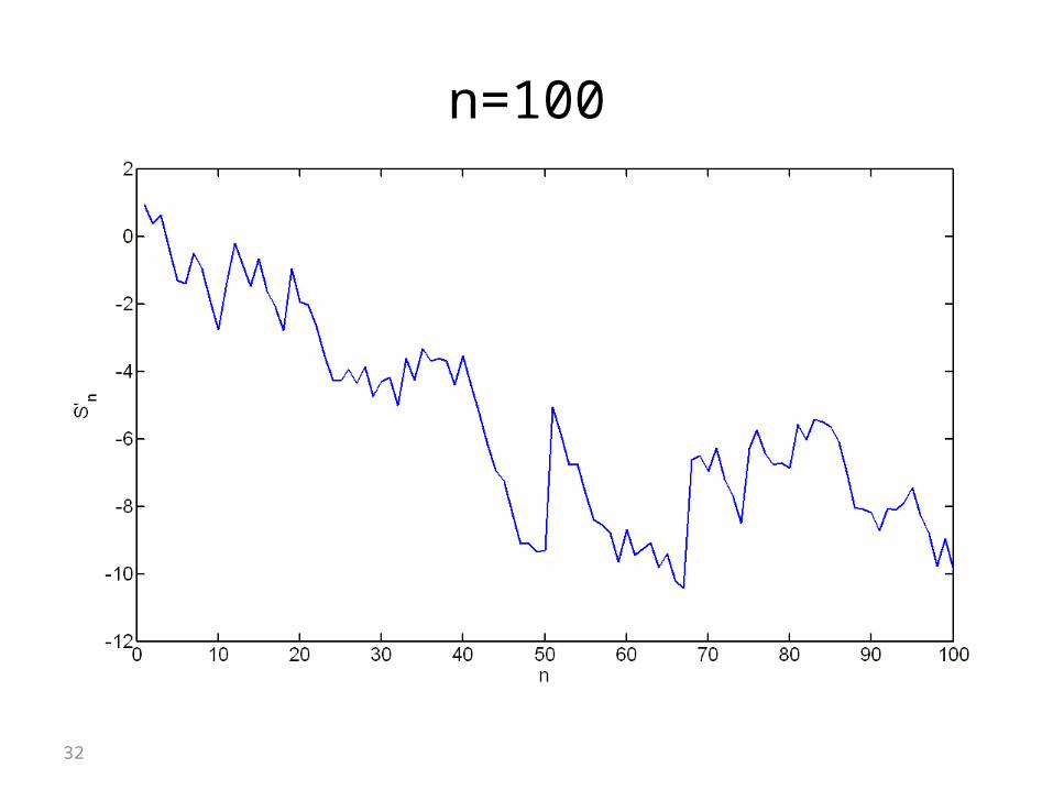
n=100

32

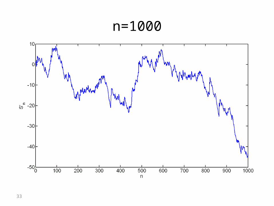
n=1000

33

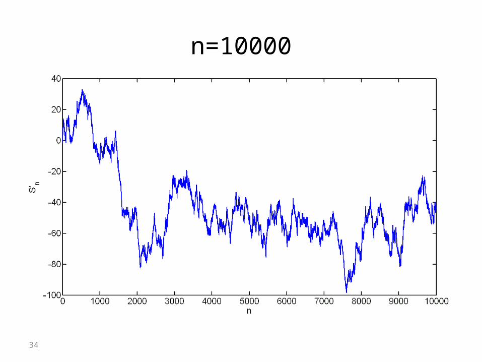
n=10000

34

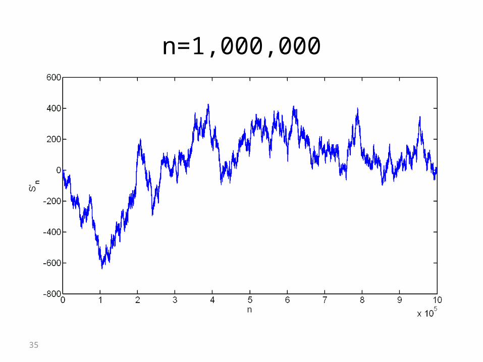
n=1,000,000

35

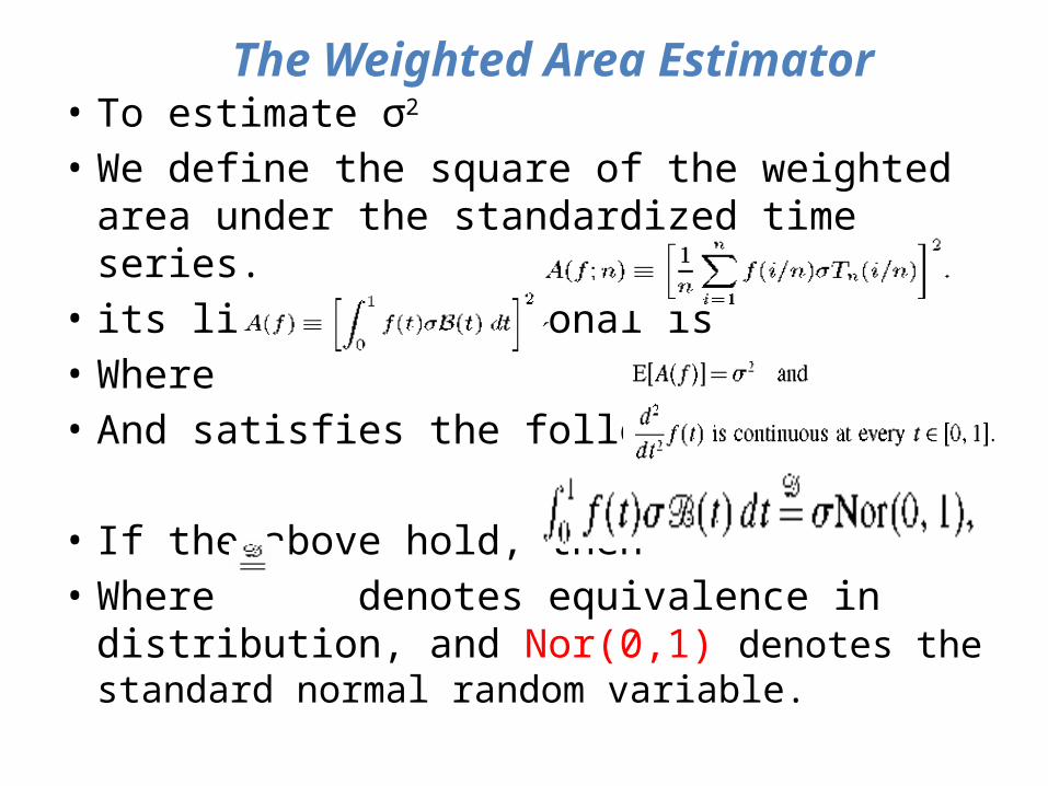
• To estimate σ2 • We define the square of the weighted area

under the standardized time series. • its limiting functional is• Where• And satisfies the following

• If the above hold, then• Where denotes equivalence in distribution,

and Nor(0,1) denotes the standard normal random variable.

The Weighted Area Estimator

The Weighted Area Estimator

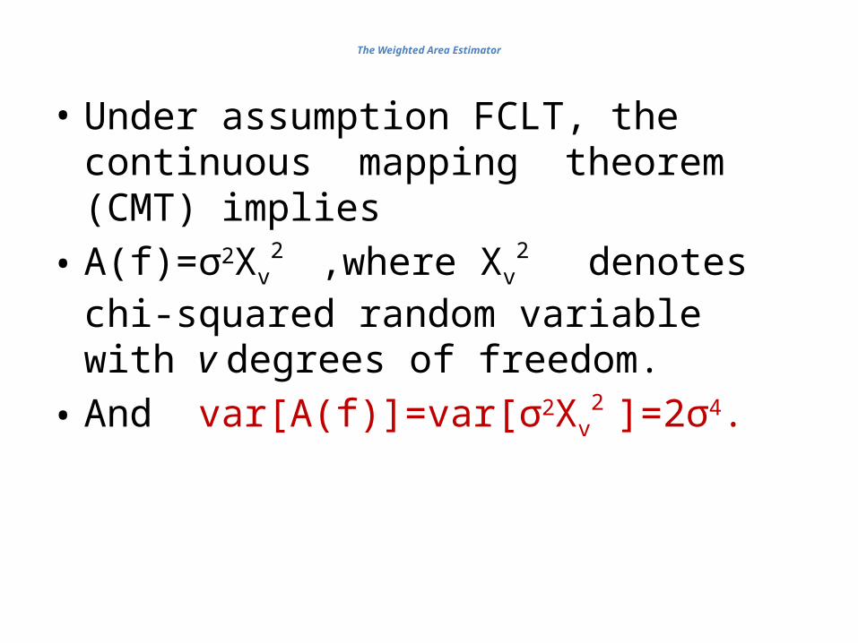
• Under assumption FCLT, the continuous mapping theorem (CMT) implies

• A(f)=σ2Xv2 ,where Xv

2 denotes chi-squared random variable with v degrees of freedom.

• And var[A(f)]=var[σ2Xv2 ]=2σ4.

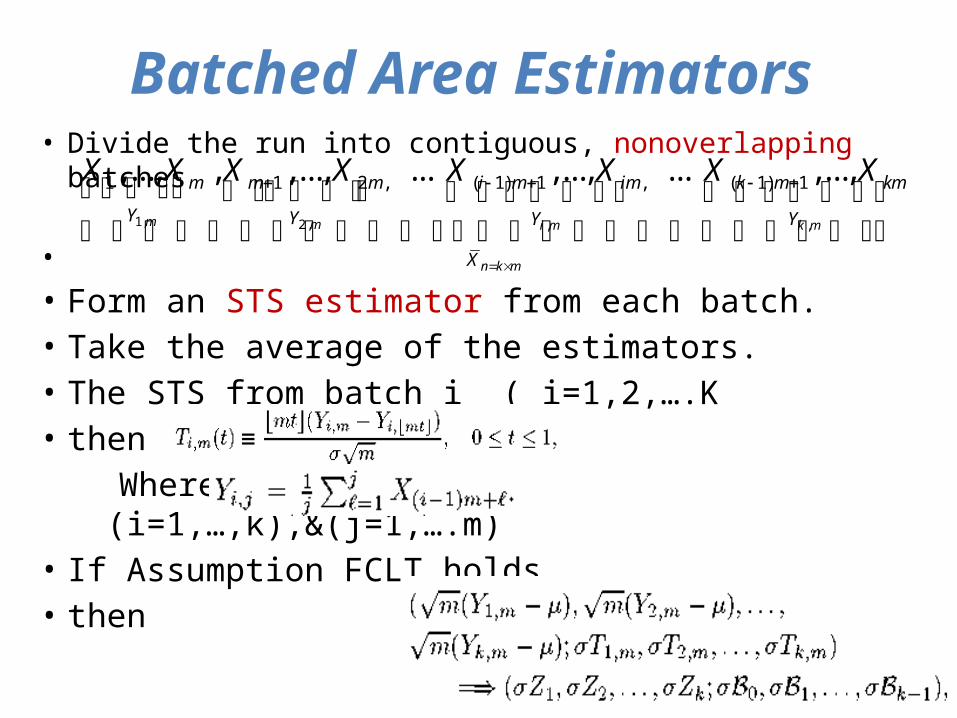
Batched Area Estimators • Divide the run into contiguous, nonoverlapping batches

• • Form an STS estimator from each batch.• Take the average of the estimators.• The STS from batch i ( i=1,2,….K • then Where (i=1,…,k),&(j=1,….m)• If Assumption FCLT holds, • then

1, 2, , ,

1 1 2 , ( 1) 1 , ( 1) 1,..., , ,..., ... ,..., ... ,...,

m m i m k m

n k m

m m m i m im k m km

Y Y Y Y

X

X X X X X X X X

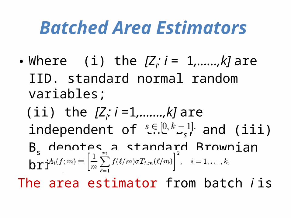
Batched Area Estimators

• Where (i) the [Zi: i = 1,……,k] are IID. standard normal random variables;

(ii) the [Zi: i =1,…….,k] are independent of the Bs; and (iii) Bs denotes a standard Brownian bridge on [s,s+1], for

The area estimator from batch i is

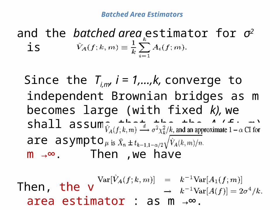
Batched Area Estimators

and the batched area estimator for σ2 is

Since the Ti,m, i = 1,...,k, converge to independent Brownian bridges as m becomes large (with fixed k), we shall assume that the the Ai (f; m) are asymptotically independent as m →∞. Then ,we have

Then, the variance of the batched area estimator : as m →∞.