Embed Size (px)
Citation preview
Taylor Rules in the Open Economy
Campbell Leith*
Simon Wren-Lewis**
*University of Glasgow
**University of Exeter
November 2002
Abstract : Taylor rules which link short-term interest rates to fluctuations in inflation and output, have been shown to be a good guide (both positively and normatively) to the conduct of monetary policy. As a result they have been used extensively to model policy in the context of both closed and open economy models. A key question that arises when analysing the conduct of such policy rules in the open economy case is whether the relevant measure of inflation is the growth in output prices or consumer prices. In this paper, we show that embedding a rule specified in terms of output price inflation into a benchmark two-country model confirms the existing result that local stability requires that the response of nominal interest rates to excess inflation should be such that real interest rates rise (the Taylor Principle), but this requirement may be partially offset by raising the interest rate response to increases in the output gap. However, all the conventional results do not hold when we replace output price inflation with consumer price inflation. In this case, Taylor rules which satisfy the Taylor principle will not support a unique rational expectations path for prices and other macroeconomic variables in response to specific shocks. Our results suggest that adoption of consumer price based Taylor rules might be chronically destabilising
JEL codes: E40, E52
Keywords: Taylor Rules, Inflation Targeting, Interest Rate Rules.
Address for correspondence: C. B. Leith, Department of Economics, University of Glasgow, Adam Smith Building, Glasgow G12 8RT E-Mail: [email protected]

2
1. Introduction
Monetary policy rules based on inflation targets are widely used in the literature, in
the context of both closed and open economy models. The best known example is the Taylor
rule (see Taylor (1993)), which takes the following form,
( ) ( )Tt t p t y t tR r m m y yπ π π= + + − + − (1)
where Rt represents the short-term nominal interest rate. The rule requires the central bank to
raise this interest rate in response to excess inflation, Ttπ π− and the output gap, t ty y− .
Taylor (op. cit.) argued that for such a rule to approximate optimal monetary policy it should
satisfy what has become known as the Taylor Principle , which states that the response of
nominal interest rates to excess inflation should be more than one for one, such that real rates
rise whenever inflation lies above its target, cet. par. That the rule should satisfy the Taylor
Principle has been confirmed more formally in the context of simple General Equilibrium
models which include nominal price rigidities (see for example, Clarida et al (1999) and
Woodford (2001)).
In extending this analysis to the open economy, a key issue is whether consumer price
inflation might be a better target than output price inflation. There are several reasons why
adopting a rule based on consumer price inflation may behave differently from a rule
formulated in terms of a measure of output prices, such as the GDP deflator. For example, the
impact of monetary policy on the exchange rate may be passed through into consumer prices
faster than monetary policy affects domestic prices through other channels of the transmission
mechanism, especially as the exchange rate can be thought of an asset price which reflects not
only current monetary policy, but also anticipated future policy. Additionally, the impact of
foreign shocks may take longer to be revealed in domestic output and inflation data, relative
to the affect they have on consumer price inflation through the exchange rate. (See Svensson
(2000) for a discussion of this and related issues.) In practice all central banks implementing
inflation targeting have chosen a consumer price-based measure of inflation.
Empirical work which seeks to estimate Taylor rules as a means of describing and
evaluating past policy has not reached a conclusion on this issue. For example, the original
Taylor rule (Taylor, op. cit.) is specified in terms of output prices in the form of the GDP
deflator. This measure is also adopted in the empirical work of, for example, Fair (2000),
McCallum (2000) and Orphanides (2001). However, it is as least as common for the rule to be
specified in terms of CPI inflation – see for example, Clarida et al (1998), Gerlach and
Schnabel (2000) and Altavilla (2000). A rare example of where the two measures are
compared is, Clarida et al (2000), who show that replacing an output-price definition of
3
excess inflation with CPI inflation does not significantly alter the estimated coefficients of a
Taylor-type rule describing US monetary policy.
At the same time a related theoretical literature has attempted to characterise optimal
monetary policy in the context of small country open economy models 1. In deriving optimal
monetary policy rules for a benchmark small open economy model, Clarida et al (2001) argue
that the policy maker’s problem is isomorphic to that in the closed economy case, and that
optimal monetary policy should, therefore, follow a simple Taylor rule, with excess inflation
defined in terms of output price inflation. Essentially this paper argues that monetary policy
should seek to minimise the distortions caused by nominal inertia (the only uncompensated
distortion in the model) in an attempt to recreate the equilibrium that would emerge under
flexible prices. Since the nominal inertia is assumed to only apply to output prices then this
should be the appropriate target for monetary policy. Subsequent work has suggested that
relaxing some of the assumptions underpinning this benchmark model, say, for example, by
allowing for stickiness or incomplete exchange-rate pass-through in the setting of import
prices, may result in open economy variables, such as the exchange rate, entering into the
optimal monetary rule (see, for example, Corsetti and Pesenti (2001), Monacelli (1999) and
Kara and Nelson (2002)). However, even in the benchmark model, where monetary policy
need only compensate for domestic price stickiness, there is no suggestion that adopting an
alternative definition for target inflation would fundamentally destabilise the economy.
In this paper we argue that, in the context of a two country model where PPP holds
for consumer prices but not output prices (as in Obstfeld and Rogoff (1996) for example), if
both countries implement Taylor rules which satisfy the Taylor Principle, defining excess
inflation in terms of consumer prices will result in indeterminacy, such that there will not be a
unique rational expectations path for prices. This indeterminacy does not arise if each
economy targets output price inflation. This implies that adoption of Taylor rules based on
consumer price inflation may not just be sub-optimal, but may be chronically destabilising.
In section 2 we develop a version of the Obstfeld-Rogoff model (op cit), which is
widely used in the literature. We augment that model in three ways. First, we relax the
assumption that consumers are infinitely lived, by introducing a fixed probability of death.
This prevents monetary policy shocks having permanent real effects. Second, we introduce a
rudimentary government sector, so that consumers in both countries can hold positive
quantities of government debt, but where fiscal policy does not induce any changes in
aggregate demand following a shock. Third, we introduce nominal inertia via Calvo (1983)
contracts, which motivates the need for a monetary policy rule. In section 3 we demonstrate
1 Benigno and Benigno (2001) and Clarida et al (2002) consider the desirability of co-ordinating monetary policies in the context of a two country model. However, the fundamental stabilising
4
the key results of the paper, using the benchmark model developed in section 2. Section 4
concludes.
2. A Two-Country Model under flexible exchange rates.
In this section we augment the two country model of Obstfeld and Rogoff (1996) -
henceforth O-R - so that we can use it to analyse the stability of alternative monetary policy
rules.
The Consumer’s Problem
Consider the utility of a typical home consumer, i, who consumes from a basket of
consumption goods, derives utility from real money balances and provides labour services,
2[ln( ) ln( ) ( ) ]exp( ( )2
ii i is
t t t s s
st
ME U E c N s t ds
Pκχ β
∞
= + − − −∫ (2)
where β is the individual’s discount rate (discussed below) and the basket of consumption
goods is defined by the following CES index applied across home and foreign goods,
11
1
0
[ ( ) ]i is sc c z dz
θ θ
θ θ
−
−= ∫ (3)
Similarly, the consumer price index is given by,
11
1 1
0
[ ( ) ]sP p z dzθ θ− −= ∫ (4)
Since there are assumed to be no impediments to trade, the law of one price holds for each
individual good, so that the Home price index can be re-written as,
11
1 * 1 1
0
[ ( ) ( ( )) ]n
s s s s
n
P p z dz p z dzθ θ θε− − −= +∫ ∫ (5)
where p(z) is the home currency price of good z, p*(z) is the foreign currency price of good z
and ε is the nominal exchange rate (where a rise represents a depreciation for home).
In O-R consumers are infinitely lived. As the authors show, this means that
temporary, asymmetric changes in monetary policy lead to permanent changes in the real
economy, because the distribution of wealth between the two economies changes. As we wish
to analyse the ability of interest rate rules specified in terms of alternative definitions of
excess inflation to stabilise the economy in the face of various shocks it is helpful to avoid
this result, by introducing the possibility that consumers have finite lives. This then ensures
properties of interest rate rules under alternative definitions of excess inflation are not considered in these papers.

5
that there is a unique steady-state which any viable interest rate rule must return our
economies to following a temporary shock. The uniqueness of this steady-state will then
allow us to compare the stabilising properties of alternative interest rate rules in a consistent
manner. Specifically, we follow Blanchard (1985) and assume that consumers face a constant
instantaneous probability of death, k , so that consumers discount future utility at the rate,
kσ + , where σ is the rate of time preference in the absence of the probability of death and
the effective interest rate faced by consumers in borrowing/lending and discounting their
future labour income is given by, tr k+ .
The consumer can hold her financial wealth in the form of domestic government
bonds, foreign bonds, and money balances. Since PPP holds at all points in time, the ex ante
real rates of return on domestic and foreign bonds will be the same, such that *t tr r= .
Additionally, we assume that all debt is fully indexed such that surprise inflation will not
affect the real rate of return on the consumer’s interest bearing financial wealth, cet. par.
Domestic consumers receive a share in the profits of domestic firms, tΠ . It is assumed that
the consumer receives a premium from perfectly competitive insurance companies in return
for their financial assets should they die. This effectively raises the rate of return from holding
financial assets by k . Consumers earn a real wage, wt and pay real lump sum taxation of tτ .
Therefore, the consumer’s budget constraint, in real terms, is given by,
**( )( ) ( )
( )
i i i i it t t t t t t
t tt t t t t
ii it t
t t t t tt t
A A M F Fd r k r k
P P P P P
Mk w N c
P P
ε ε
π τ
= + − − + +
Π+ − + + − −
(6)
where itA represents consumer i’s financial assets, which can either be held as domestic
bonds, as money, itM or in the form of foreign bonds, *i
tF .
The consumer than has to maximise utility (2), subject to their budget constraint (6)
along with the standard solvency conditions. The various first order conditions this implies
are given below. Firstly, there is the usual consumption Euler equation,
( )i it t tdc r cσ= − (7)
The optimisation also yields a money demand equation,
i it t
t t
M cP R
χ= (8)
where tR is the nominal interest rate. The individual’s optimal labour supply decision will
satisfy,
1i t
t it t
WN
P c κ= (9)
6
Integrating the consumer’s Euler equation forwards and substituting into the
intertemporal budget constraint yields the fully solved out version of the consumption
function,
( )( ( )exp( ( ( ) ) )si
i it s st s s
t s st t
A Wc k N r k d ds
P P Pσ τ µ µ
∞ Π= + + + − − +∫ ∫ (10)
If we normalise total population size to one, then it is possible to aggregate across
generations by noting that the current size of a generation of size k when born at time z is
exp( ( ))k k z t− . Therefore, for example aggregate consumption is given by,
exp( ( ))t
it tc c k k i t di
−∞
= −∫ (11)
Applying this aggregation to all variables allows us to derive the aggregate domestic
consumption function as,
( )( ( )exp( ( ) )s
t s st s s
t s st t
A Wc k N r k d ds
P P P µσ τ µ∞ Π= + + + − − +∫ ∫ (12)
where the aggregate financial wealth of domestic consumers is made up of their holdings of
money, domestic bonds and foreign bonds, *t t t tA M D F= + + .
The relationship between aggregate per capita labour supply and the real wage is
given as2,
1
exp( ( ))t
tt i
t t
WN k k i t di
P cκ −∞
= −∫ (13)
While the money demand equation is given by,
t t
t t
M cP R
χ= (14)
In the foreign country there will be corresponding equations for labour supply, money
demand and consumption.
The Firm’s Problem
Firms are assumed to maximise the discounted value of their profits. In the absence of
capital and without any constraints on price setting the firm would simply maximise profits in
each period in a static manner. However, it is assumed that firms are subject to the constraints
implied by Calvo (1983) contracts such that at each point in time firms are able to change
prices with a probability α . As firms cannot adjust their prices continuously, there is an
2 In general the non-linear formulation of the labour supply decision means that a simple aggregation in terms of per capita aggregates is not possible. However, upon log-linearisation this equation can be represented in terms of percentage deviations from steady-state of aggregate variables.

7
intertemporal dimension to the firm’s pricing/output decision. Suppose the firm is able to
change its current price, then its objective function for determining its optimal value is given
by,
( )
( ) [ ( ) ( ) ](exp( ( ) )s
s st s s
s st t
p z WV z y z N z r d ds
P P µ α µ∞
= − − +∫ ∫ (15)
For simplicity it is assumed that the firms production technology is linear, ( ) ( )t ty z N z= . The
CES form of the utility function implies that the ith consumer’s demand for product z is given
by,
( )
( ) i itt t
t
p zc z c
P
θ−
=
(16)
Integrating demands across consumers and assuming that the home government allocates its
spending in the same pattern as home consumers implies that world demand for product z is
given by,
* *( )( ) ( )t
t t t t tt
p zy z c c g g
P
θ−
= + + +
(17)
where y(z), c, c*, g, and g* are defined as real per capita variables. Given the linear
production function, the firm’s (per capita) demand for labour will be equivalent to equation
(17).
Utilising the home and foreign demands for product z, allows us to rewrite the firm’s
objective function as,
* *( ) ( )( ) [ ( )](exp( ( ) )
ss s s
t s s s ss s st t
p z W p zV z c c g g r d ds
P P P
θ
µ α µ−∞
= − + + + − +
∫ ∫ (18)
where the discount rate is raised by the instantaneous probability α to reflect the fact that this
price may be in force for some time.
The optimal price implied by the maximisation of this objective function is therefore
given by,
1
* *
1
* *
1( )exp( ( ) )
( )
1( 1) ( )exp( ( ) )
s
s s s s sst t
t
s
s s s st st t
W c g c g r d dsP
p z
c g c g r d dsP
θ
µ
θ
µ
θ α µ
θ α µ
−∞
−∞
+
+ + + − +
=
− + + + − +
∫ ∫
∫ ∫
(19)
The home output price index, ( )tp h is a weighted average of the prices set in the
past, where the weights reflect the probability that these prices are still in existence,
11
1( ) [ exp( ( )) ]t
t sp h p t s dsθ
θα α−
−
−∞
= − −∫ % (20)
8
where tp% is the price set in accordance with equation (19) by those home producers that were
able to change prices at that point in time. The aggregate consumer price level is, in turn,
given by,
1
1 1 1[ ( ) (1 )( ( ) ) ]t t t tP np h n p fθ θ θε− − −= + − (21)
Home output is given by,
* *( )( ) ( )t
t t t t tt
p hy h c g c g
P
θ−
= + + +
(22)
which, given the linear production technology, means that demand for labour is obtained by
summing across the n home firms,
* *( )( )t
t t t t tt
p hN n c g c g
P
θ−
= + + +
(23)
The Government
The home government’s budget constraint, in real terms, is given by,
( )t t t t t t t tdl r l m m gπ τ= − − + − (24)
where the total liabilities of the government, lt are made of government bonds held by home
consumers (dt) or by foreign consumers ( *tf ), and non-interest bearing money, mt. Aside from
borrowing and seigniorage, the government finances spending by levying a lump-sum tax of
tτ on home consumers.
The introduction of a probability of death, which was necessary to generate a unique
steady-state, implies that government debt is an element of net wealth and that Ricardian
Equivalence does not hold. As a result there may be interactions between monetary and fiscal
policy when stabilising the economy following a shock.3 However, since the focus of this
paper is on the specification of the monetary policy rule, we wish to formulate fiscal policy in
such a way that it does not directly affect the macroeconomic outcomes in our economies.
The simplest way of achieving this is by assuming that government spending is constant and
that lump-sum taxation is adjusted to ensure that the real value of government liabilities
remain at their steady-state level, such that,
t t t tg r l R mτ = + − (25)
This means that there is no delay in adjusting taxation to ensure that government debt remains
at its steady-state level and that fiscal policy does not affect aggregate demand even although
consumers face a probability of death. Additionally, the fact that government debt is indexed
9
and fiscal policy is clearly solvent, means that we can ignore the complications that the Fiscal
Theory of the Price Level creates for the conduct of monetary policy (for a summary see
Woodford (2001)). Similar policies are followed in the foreign economy.
Appendix I details the log-linearisation of the model around its steady-state. We now
consider the implications of adopting different definitions of excess inflation in monetary
policy rules of the Taylor form.
3.Defining Excess Inflation in the Taylor Rule
Monetary Policy Targeting Output Price Inflation
In this subsection we assume that monetary policy follows a Taylor rule which
specifies excess inflation in terms of output prices. Monetary policy in both economies
involves setting nominal interest rates to target domestic output price inflation such that,
ˆ ˆ ˆ(1 ) ( )t op t y trR m h m yπ= + + (26)
and,
* * * *ˆ ˆ ˆ(1 ) ( )t op t y yrR m f m yπ= + + (27)
where a hatted variable denotes percentage deviation from steady-state as defined in
Appendix I.
We then embed these rules into our log-linearised two country model, which allows
us to write the model in matrix form as,
ˆ ˆtd = tx Ax (28)
where ' *ˆ ˆ ˆ ˆ ˆ ˆ ˆ[ ( ) , ( ) , , , , ]t t t t t t th h e c c aπ π=x is a vector of six endogenous variables4, and A is the
transition matrix detailed in Appendix II, whose elements are combinations of the underlying
structural parameters of the model, and which describes the dynamic evolution of our two
economies.
Necessary Conditions for Saddle-Path Stability
The question we now pose is which values of the monetary policy parameters opm
and *opm ensure that the model will deliver saddlepath stability? In other words can we
identify the conditions under which policy will generate a unique path for prices under
3 For an analysis of such interactions in the context of a similar open economy model see Leith and Wren-Lewis (2002), which extends the closed economy analysis of Leith and Wren-Lewis (2000).

10
rational expectations and ensure that both countries return to their steady-state values
following a temporary shock?
With a flexible exchange rate and forward-looking price-setting and consumption
behaviour, the only predetermined variable in the system is financial wealth, ˆta . The
remaining five variables are ‘jump’ variables. Saddlepath stability requires there to be as
many eigenvalues with positive real parts as there are ‘jump’ variables. The necessary
condition for saddlepath stability is, therefore, that the determinant is negative. In the general
case the determinant of the transition matrix is quite complex. However, it can be simplified
by assuming that *y ym m= . Under this simplifying assumption the determinant becomes,
* *[1]( ) ( [2] [3] )( ) [4] ( (1 ))op op y op op y y
gA m m A A m m m A m r m
yσ− − + + − − + − (29)
where [ ] 0A i > , i=1,..4 are expressions combining the structural parameters of the model, but
which are not a function of the parameters of the policy rules. These expressions are defined
in Appendix III, where they are also shown to be positive. This expression reveals that
positive coefficients on excess inflation and the output gap in the monetary policy rules of the
two economies will ensure a negative determinant consistent with saddlepath stability. The
expression also shows that there are potential interactions between policy parameters in
achieving saddlepath stability. To see this we solve the determinant condition for the two
policy coefficients on excess inflation to give,
( [2] [3] ) [4]( (1 ))
[1] [2] [3]
jy op y
iop j
op y
gA A m m A r m
ym
A m A A m
σ+ + − + −> −
+ + (30)
and [2] [3]
[1]yj
op
A A mm
A
+> − (31)
where i and j refer to the respective monetary authorities5.
The conditions in equations (30) and (31) can be represented diagrammatically as the
area to the right of the parabola in Figure 1, which has been drawn under the assumption that
0ym = .
4 The model can be reduced to a dynamic system in six variables by using the market clearing conditions in the goods and bonds markets as shown in Appendix II. 5 There are corresponding conditions with the signs reversed (i.e when opm strongly violates the Taylor
principle), but numerical evaluation of the eigenvalues (see footnote 6 below) suggests that although this satisfies the determinant condition it does not deliver saddlepath stability.
11
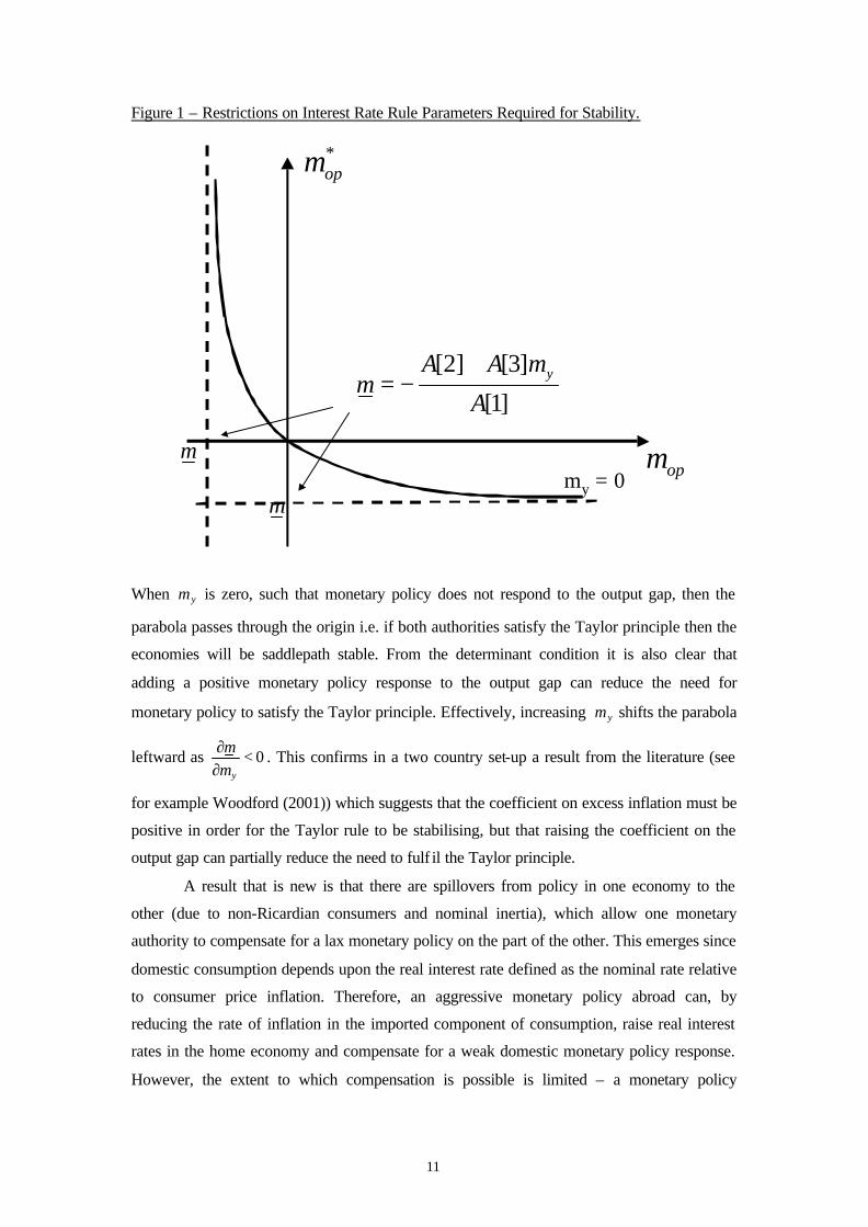
Figure 1 – Restrictions on Interest Rate Rule Parameters Required for Stability.
When ym is zero, such that monetary policy does not respond to the output gap, then the
parabola passes through the origin i.e. if both authorities satisfy the Taylor principle then the
economies will be saddlepath stable. From the determinant condition it is also clear that
adding a positive monetary policy response to the output gap can reduce the need for
monetary policy to satisfy the Taylor principle. Effectively, increasing ym shifts the parabola
leftward as 0y
mm∂ <
∂. This confirms in a two country set-up a result from the literature (see
for example Woodford (2001)) which suggests that the coefficient on excess inflation must be
positive in order for the Taylor rule to be stabilising, but that raising the coefficient on the
output gap can partially reduce the need to fulf il the Taylor principle.
A result that is new is that there are spillovers from policy in one economy to the
other (due to non-Ricardian consumers and nominal inertia), which allow one monetary
authority to compensate for a lax monetary policy on the part of the other. This emerges since
domestic consumption depends upon the real interest rate defined as the nominal rate relative
to consumer price inflation. Therefore, an aggressive monetary policy abroad can, by
reducing the rate of inflation in the imported component of consumption, raise real interest
rates in the home economy and compensate for a weak domestic monetary policy response.
However, the extent to which compensation is possible is limited – a monetary policy
[2] [3]
[1]yA A m
mA
+= −
m
m
opm
*opm
my = 0

12
parameter iopm m< cannot be compensated for by increasing the responsiveness of monetary
policy in the second economy.
Overall, our analysis of Taylor rules using excess inflation defined in terms of output
prices, in the context of a benchmark two country model with nominal inertia, confirms and
extends results already detailed in the literature. Satisfying the Taylor principle allows the
rules to generate a unique equilibrium path for prices. Allowing monetary policy to respond to
deviations of output from equilibrium can, partially, mitigate the need to satisfy the Taylor
principle. We also find that policy spillovers imply that one monetary authority can
compensate to a limited degree for a relatively weak monetary response to inflation in another
economy.
Monetary Policy in Both Economies Targeting Consumer Price Inflation
We now assume that the monetary policy of the both economies involves setting nominal
interest rates to target consumer price inflation so that,
ˆ ˆ ˆ(1 )t cp t y trR m m yπ= + + (32)
and,
* * * * *ˆ ˆ ˆ(1 )t cp t y trR m m yπ= + + (33)
Appendix IV details the dynamic system under this monetary policy specification. The
determinant of the transition matrix when the interest rate rule is defined in terms of consumer
price inflation is given by,
*
* *
( )2 [1] 2( [2] [3] ) 2 [4] ( (1 ))cp cp y
y ycp cp cp cp
m m m gA A A m A r m
m m m m yσ+ + + − + −
+ + (34)
Now suppose that we consider the set of parameter values such that op cp pm m m= =
and * * *op cp pm m m= = , in other words we condition on the strength of the monetary policy rule,
so that the only difference is the price measure targeted. It is then straightforward to show that
the ratio of the determinants of the two transition matrices when excess inflation is defined in
terms of consumer and output prices, respectively is given by,
*
2
p pm m−
+ (35)
In other words, a combination of positive feedback parameters which ensures
saddlepath stability in the case of output price inflation, will unambiguously fail to do so
when excess inflation is defined in terms of consumer prices, since the sign of the determinant
of the transition matrix of the underlying dynamic system changes. It is therefore the case that
the results shown above for output price inflation are reversed by simply changing the
13
definition of excess inflation from output price inflation to consumer price inflation. In
particular, Taylor rules using consumer prices that satisfy the Taylor principle will no longer
stabilise the two economies6. Furthermore, it is not possible for the monetary authorities to
alter the coefficient on the output gap to compensate for the instability induced by targeting
consumer price inflation in the Taylor rule.
Monetary Policy in One Economy Targeting Consumer Price Inflation
The final case we consider is where the home economy targets consumer price
inflation,
ˆ ˆ ˆ(1 )t cp t y trR m m yπ= + + (36)
while the foreign economy targets output price inflation7,
* * * *ˆ ˆ ˆ(1 ) ( )t op t y yrR m f m yπ= + + (37)
Details of the dynamic system under this combination of policy rules is given in Appendix V.
However, the key result is that the ratio of the determinants when both countries target output
price inflation, relative to the case where one economy adopts a CPI inflation target is given
by,
2
1 pm− (38)
Therefore, if a country is aggressively targeting CPI inflation, such that the coefficient on
excess inflation in a Taylor rule is greater than one, then this will also lead to indeterminacy.
To understand the intuition behind these results, it is helpful to remove the output gap
term and concentrate solely on the consequences of changing the definition of excess
inflation.
Rules reacting to Inflation Alone
In order to highlight the differences between output price and CPI inflation targeting
in the context of Taylor rules, we shall consider the uniqueness or otherwise of the dynamic
path towards the unique steady-state. We shall initially describe a dynamic path that returns
6 Of course the analysis of the determinant only gives us necessary conditions for saddlepath stability. However, numerical analysis of the eigenvalues of the dynamic system using a plausible parameter set described in Leith and Wren-Lewis (2002) confirms that monetary policy rules based on output price inflation which satisfy the Taylor principle will be saddlepath stable. However, when we turn to the case of consumer price inflation, any combination of positive inflation feedback parameters implies that there are too many stable roots – we are faced with the problem of indeterminacy. 7 Since the two economies are otherwise symmetrical, consideration of this final case implies that we have covered all possible permutations of definitions of excess inflation across our two rules/economies.

14
our economies to equilibrium following an asymmetric shock. We shall then consider whether
or not deviations from the initial jumps in variables assumed as part of this dynamic path
imply that we fail to reach the equilibrium. In the case of output price inflation targeting, we
shall see that deviating from our equilibrium path implies that our economies evolve along an
explosive trajectory, while in the case of CPI inflation targeting a return to equilibrium will
still be achieved. In other words, there is a unique saddle -path equilibrium under output price
inflation targeting, but indeterminacy under CPI inflation rules.
Intuition is clearer if we assume that the wealth effects in our model are negligible.
Without wealth effects, then after the shock has ended the economy must have returned to
steady-state8. The particular shock we consider is a preference shock, which temporarily
raises demand for home goods relative to foreign. Given our forward-looking Phillips curves,
equations (58) and (59), with excess demand (supply) at home (abroad) output price inflation
must be falling (rising) at home (abroad). Since, inflation in both economies must return to
equilibrium once the shock is over, these inflation paths determine the initial inflation jumps
(positive at home, negative overseas) necessary to restore equilibrium once the shock has
passed.
A key issue is what happens to the real exchange rate (competitiveness) during and
after this shock. This is because, under PPP, real interest rates are equalised across our two
economies, so the only way of deflating the home economy relative to the foreign is to induce
a real exchange rate appreciation. By combining the definitions of home and foreign GDP,
equations (70) and (71), we can relate the difference between home and foreign output to the
real exchange rate,
*ˆ ˆ ˆt t ty y eθ− = (39)
With no change in nominal interest rates, the nominal exchange rate would jump to a
new equilibrium level which is consistent with the steady state level of the real exchange rate
i.e. a nominal depreciation from the home country’s point of view. However, to the extent that
higher inflation at home results in higher nominal interest rates at home relative to abroad,
then monetary policy will pull the exchange rate in the opposite direction. Critically, the sign
of the net effect depends on whether output or consumer price inflation is targeted.
Consider targeting output price inflation first. The dynamics of the exchange rate are
given by,
8 If the wealth effects introduced through our infinitely lived consumers are significant, then changes in the distribution of financial wealth between the two consumers can prolong the effects of a given shock. Once the shock has passed, to the extent that one country has accumulated the financial wealth of the other, there will be inflationary pressure in that country while finitely lived consumers run-down their holdings of net foreign assets. However, the uniqueness, or otherwise, of the saddlepath can still be considered by analysing the behaviour of inflation and the exchange rate when the initial jumps in these variables are different from an assumed dynamic path which reaches the steady-state.
15
*ˆ ˆ ˆ( ) ( )t op t op tde m h m fπ π= − (40)
As long as the Taylor principle is followed, the real exchange rate will be depreciating
following the preference shock. and the effect on the exchange rate of higher home interest
rates outweighs the effect of higher output prices. Therefore, the initial shock will generate a
jump appreciation in the home real exchange rate, followed by a depreciation towards
equilibrium as inflation unwinds. Suppose, however, that home (overseas) inflation is still
above (below) equilibrium once the shock is over. Equation (40) tells us that if the real
exchange rate is to return to equilibrium, then the home real exchange rate must be
appreciated relative to its steady-state value. This appreciation will be reducing (raising)
demand for home (foreign) goods. However, with a forward-looking Phillips curve, these
changes in demand will be raising (reducing) home (overseas) inflation9. Thus by deviating
from the assumed equilibrium path, the economy will fail to reach the steady-state. Therefore,
there is a unique saddlepath which will return the economy to equilibrium for a given shock,
under rules specified in terms of output price inflation.
Now consider consumer price inflation targeting. The nominal interest rate
differential is given by
* * *ˆ ˆ ˆ ˆ(1 ) (1 )t t cp t cp tR R m mπ π− = + − + (41)
Using the definition of consumer price inflation and the UIP condition for the nominal
exchange rate, this can be rearranged as,
*
*
*ˆ ˆ ˆ ˆ( ( ) ( ) )cp cp
t t t t
cp cp
m mR R h f
m mπ π
−− = +
+ (42)
Differentiating the definition of the real exchange rate with respect to time, and utilising
equation (42) reveals that the dynamics for the real exchange rate are given by,
*
*
*
* *
ˆ ˆ ˆ ˆ ˆ( ) ( ) ( ( ) ( ) )
2 2ˆ ˆ( ) ( )
cp cpt t t t t
cp cp
cp cpt t
cp cp cp cp
m mde h f h f
m m
m mh f
m m m m
π π π π
π π
−= − + + +
+
= − ++ +
(43)
Notice that the signs of the coefficients on home and foreign inflation in the equation of
motion for the real exchange rate are now reversed in the case of CPI-based rules.
The initial inflation shock will now generate a jump depreciation in the home real
exchange rate, followed by a appreciation towards equilibrium while the shock lasts. Suppose,
however, we deviate from the equilibrium path, so that home (foreign) inflation is still
positive (negative) once the shock has passed. Equation (43) implies that the real exchange
rate must be appreciating. For this to remain consistent with attaining the steady-state the real
9 Note the opposite is true when inflation is determined in a backward-looking manner, but this is exactly what is required when inflation is considered to be a predetermined variable.
16
exchange rate must be depreciated relative to equilibrium, raising (lowering) the demand for
home (overseas) goods. In the context of forward-looking Phillips curves this implies that
home (foreign) output price inflation is falling (rising) , so that we can also reach the steady-
state following this alternative dynamic path10. In other words, there are multiple paths to the
steady-state, which leaves the price level undefined. CPI-inflation based rules generate
indeterminacy in the context of our benchmark two-country model.
In the case where one economy (in this case home) targets CPI inflation and the other
economy (foreign) targets output price inflation the interest rate differential can be shown to
be,
* *
* 1 1 ( )ˆ ˆ ˆ ˆ( ) ( )1 1
cp op op cpt t t t
cp cp
m m m mR R h f
m mπ π
+ + + −− = −
− − (44)
The numerators of these expressions capture the ‘direct’ impact of output price inflation in the
two economies on the monetary policies of the two economies. It is clear that monetary policy
in the home country responds to both domestic and foreign inflation, while the foreign
economy reacts only to output price inflation in that economy. As a result the impact of
foreign inflation on the interest rate differential, depends not only on monetary policy in the
foreign economy, but on the extent to which the home monetary authorities offset that policy.
However, the interesting factor in this expression is the numerator, 1 cpm− , which captures
the repercussions of the monetary policy response to home and foreign inflation on the
exchange rate which then feeds through into home CPI inflation. Accordingly, when the home
country aggressively targets CPI inflation, 1cpm > , exchange rate movements can dominate
the setting of monetary policy, such that an inflationary shock in the home country actually
leads to a reduction in the nominal interest rate differential. This then prevents the monetary
authorities engineering the real exchange rate appreciation required to disinflate the home
economy. We can also note that this reasoning goes through for the home economy even if
overseas monetary policy and inflation are fixed.11
The logic of these arguments requires only that an appreciated real exchange rate
deflates the demand for goods. The intertemporal behaviour of consumers is not critical here.
In fact, it is possible to demonstrate these stability results in a simpler (but less satisfactory)
model in which consumption responds statically to real interest rates, labour supply is fixed
and an appreciation in the real exchange rate reduces demand for domestic output. In addition,
as noted above, the result also carries over into a world where prices are set by backward-
10 Again this logic is reversed when inflation is considered to be a predetermined variable, set according to a backward-looking rule of thumb. 11 See Linnemann and Schabert (2001) who generate a similar result for a small open economy.
17
looking rules of thumb, and inflation is determined by a traditional accelerationist Phillips
curve.
To obtain this clear-cut result we relied on two key features of the model: PPP and the
lack of any ‘home bias’ in consumption patterns in the two economies. However, even if we
relax these assumptions, the basic mechanism underlying the different outcomes under the
two rules would still come through to some extent. As long as there is some pass-through
from the exchange rate to consumer prices, then relying on a rule specified in terms of
consumer prices will lessen the ability of one economy to disinflate relative to another
following a given asymmetric inflationary shock. If the degree of openness of the economy is
large enough and the pass-through from the exchange rate to consumer prices sufficiently
fluid then we may continue to observe that Taylor rules specified in terms of consumer price
inflation are destabilising.
4.Conclusions
In this paper we considered the ability of Taylor rules to stabilise a standard ‘new
open economy macroeconomics’ description of the open economy. We found that much of
the analysis of closed economy Taylor rules applies to the open economy when the excess
inflation term in the rule is specified in terms of output prices. The only major difference,
relative to the closed economy or small open economy cases, was that failure to fulfil the
Taylor principle on the part of one monetary authority could be partially offset by a more
active monetary policy on the part of the monetary authority in the second economy.
However, if the Taylor rule was specified in terms of consumer price inflation (as is
frequently the case), these conventional results no longer held. Rules which satisfied the
Taylor principle, and which were consistent with estimated policy reaction functions, but
which targeted CPI inflation, would not deliver a unique rational expectations path for prices.
Our results imply that adoption of Taylor rules based on consumer rather than output price
inflation may be chronically destabilising. Therefore, to the extent that Taylor rules are a
reasonable description of central bank behaviour, the fact that more central banks are adopting
explicit inflation targets based on consumer prices should be a cause for concern.
18
References:
Altavilla, C. (2000), “Assessing Monetary Rules Performance across EMU Countries”, mimeograph, University of Leuven. Ball, L. (1998), “Policy Rules for Open Economies”, NBER Working Paper No. 6760. Benigno, G. and P. Benigno (2001), “Implementing Monetary Cooperation through Inflation Targeting”, mimeograph, Bank of England. Clarida, R., J. Gali and M. Gertler (1998), “Monetary Policy Rules in Practice. Some International Evidence”, European Economic Review, No. 42, pp 1033-1067. Clarida, R., J. Gali and M. Gertler (1999), “The Science of Monetary Policy: A New Keynesian Perspective”, Journal of Economic Literature, Vol. XXXXVII, pp 1661-1707. Clarida, R., J. Gali and M. Gertler (2000), “Monetary Policy Rules and Macroeconomic Stability: Evidence and Some Theory”, Quarterly Journal of Economics, pp. 147-180. Clarida, R., J. Gali and M. Gertler (2001), “Optimal Monetary Policy in Open Economies: An Integrated Approach”, American Economic Review, Vol, pp Clarida, R., J. Gali and M. Gertler (2002), “A Simple Framework for International Monetary Policy Analysis”, mimeograph, Columbia University. Corsetti, Giancarlo and Paolo Pesenti (2001). “The International Dimension of Optimal Monetary Policy”. NBER Working Paper No. 8230. Erceg, C. J., D. W. Henderson and A. T. Levin (2000), `Optimal Monetary Policy with Staggered Wage and Price Contracts', Journal of Monetary Economics 46, pp281-313. Freedman, C. (1996), “What Operating Procedures Should be Adopted to Maintain Price Stability – Practical Issues”, in Achieving Price Stability – A Symposium Sponsored by the Federal Reserve Bank of Kansas City, Pub Federal Reserve Board of Kansas City. Gerlach, S. and G. Schnabel (2000), “The Taylor Rule and Interest Rates in the EMU Area”, Economics Letters, 46, pp165-171. Kara, A. and E. Nelson (2002), “The Exchange Rate and Inflation in the UK”, mimeograph, Bank of England. Leith, C. and S. Wren-Lewis (2000), “Interactions Between Monetary and Fiscal Policy Rules”, Economic Journal, Vol 110, No. 462, pp 93-108. Leith, C. and S. Wren-Lewis (2002), “Interactions Between Monetary and Fiscal Policy Under Flexible Exchange Rates”, mimeograph, University of Glasgow. Linnemann, L. and A. Schabert (2001), “Monetary Policy, Exchange Rates and Real Indeterminacy”, mimeograph, University of Cologne. McCallum, B. T. (2000), “Alternative Monetary Policy Rules: A Comparison with Historical Settings for the United States, the United Kingdom, and Japan”, NBER Working Paper No. 7725.

19
Monacelli, Tommaso (1999). “Open Economy Policy Rules under Imperfect Pass-Through”, mimeograph, New York University. Obstfeld, M. and K. Rogoff (1995), “Exchange Rate Dynamics Redux”, Journal of Political Economy, No. 103, pp 624-660. Orphanides, A. (2001), “Monetary Policy Rules, Macroeconomic Stability and Inflation: A View from the Trenches”, European Central Bank Working Paper No. 115. Svensson, L.E.O. (2000), “Open-Economy Inflatioin Targeting”, Journal of International Economics, 50, pp155-183. Taylor, J. (1993), “Discretion Versus Policy Rules in Practice”, Carnegie-Rochester Series on Public Policy, Vol 39, pp195-214. Woodford, M. (2001), “Fiscal Requirements for Price Stability”, Journal of Money, Credit and Banking No.33: pp 669-728. Woodford, M, (2001), “The Taylor Rule and Optimal Monetary Policy”, American Economic Review, 91(2), pp 232-237.

20
Appendix I – Log-linearising the model around its steady-state.
The Steady-State
In this Appendix we linearise our model around a symmetrical steady-state. We also
assume, for simplicity, that the rate of inflation in our steady-state is zero, so that the mis-
pricing due to overlapping contracts will not exist in steady-state. Equation (19) shows that
the optimal price in steady-state, which is the same as that which would be set under flexible
prices, is given by
( )1
p h Wθ
θ=
− (45)
Combining this with the labour supply condition, the linear production function and the
national accounting identity (in the symmetrical steady-state the current account will be in
balance so that y c g= + ), yields the following equilibrium output,
2 4( 1)
2
g gy N
θθκ
−± += = (46)
If government spending is set equal to zero, then this is identical to the steady-state output
found in Obstfeld and Rogoff (op. cit.).
The steady-state consumption function is given by,
( )
( )y D F M
c kr k P P
τ εσ − += + + + + (47)
The domestic government’s budget constraint becomes,
* gD F
P rτ −+ = (48)
money demand is given by,
M cP r
χ= (49)
Note that in this symmetrical equilibrium, with PPP due to free trade, it will also be the case
that the real value of debt held overseas will be the same in both countries, *F F
P Pε= . This
fact, combined with equations (46)-(49), will determine the steady-state value of real assets in
the model, along with the equilibrium real interest rate,
2(1 ) (1 )( (1 ) 4 ( )( )12 1
g g g gk k
y y y yr
gy
τσ σ σ −− + − − + +
=−
(50)

21
Since consumers are not infinitely lived, the real interest rate is not identical to consumers’
rate of time preference, but will be affected by the outstanding stock of government liabilities,
since these liabilities constitute consumers’ net wealth.
Log-Linearising the Model:
We now proceed to log-linearise the model around this symmetrical steady-state. To
illustrate this consider the labour supply equation,
1
exp( ( ))t
tt i
t t
WN k k i t di
P cκ −∞
= −∫ (51)
Taking the natural logarithm of both sides, differentiating and evaluating this expression at
the symmetrical steady-state yields,
ˆt t tN w c= −) ) (52)
Where a hatted variable denotes the percentage deviation from steady-state, ˆ t x xt
dXX
X== .
This approach can be applied to all the equations in our model.
Next, consider the linearised expression for the optimal price set by a home firm,
( )[ ]exp( ( )( )t s s
t
p r P w r s t dsα α∞
= + + − + −∫) ) )% (53)
Differentiating this expression with respect to time and substituting for the definition of
consumer prices, 1 1 1 ˆ( ) ( )2 2 2t t t tP p h p f ε= + +
) ) ) , yields,
1 1 1 ˆˆ ˆ( )( ( ) ( ) )2 2 2t t t t t tdp r p p h p f wα ε= + − − − −
) ) )% % (54)
Log-linearising the expression for the index of home country output prices gives,
ˆˆ ( ) exp( ( )) ]t
t sp h p t s dsα α−∞
= − −∫ % (55)
Differentiating with respect to time,
ˆˆ ˆ( ) ( ( ) )t t tdp h p p hα= −% (56)
Differentiating again,
ˆˆ ˆ( ) ( ( ) )
1 1 1ˆˆ ˆ ˆ ˆ( ) ( ) ( )( ( ) ( ) )
2 2 2
t t t
t t t t t
d h dp dp h
r h r w r p h p f
π α
α π α α α α ε
= −
= − + + + − −
% (57)
Substituting the linearised labour supply function and the definition of the real
exchange rate into this expression gives the open economy Phillips curve for the home
economy,
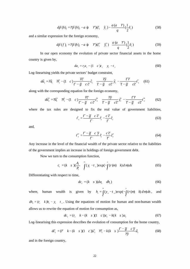
22
( ) 1
ˆ ˆ ˆ ˆ ˆ( ) ( ) ( )( ) ( )2t t t t t
rd h r h r c y e
α απ π α αθ+= − + + − (58)
and a similar expression for the foreign economy,
* * ( ) 1ˆ ˆ ˆ ˆ ˆ( ) ( ) ( )( ) ( )
2t t t t t
rd f r h r c y e
α απ π α αθ+= − + + + (59)
In our open economy the evolution of private sector financial assets in the home
country is given by,
(1 )t t t t t tda r a c yχ τ= − + + − (60)
Log-linearising yields the private sectors’ budget constraint,
ˆ ˆ ˆ ˆ ˆ ˆ(1 )t t t t t t
ryrc rda ra rr c y
g c g c g cτχ τ
τ χ τ χ τ χ= + − + + −
− + − + − + (61)
along with the corresponding equation for the foreign economy,
* * * * *ˆ ˆ ˆ ˆ ˆ ˆ(1 )t t t t t t
ryrc rda ra rr c y
g c g c g cτχ τ
τ χ τ χ τ χ= + − + + −
− + − + − + (62)
where the tax rules are designed to fix the real value of government liabilities,
ˆ ˆ ˆt t t
g c cr c
τ χ χττ τ
− += − (63)
and,
* *ˆ ˆ ˆt t t
g y cr c
τ χ χττ τ
− += − (64)
Any increase in the level of the financial wealth of the private sector relative to the liabilities
of the government implies an increase in holdings of foreign government debt.
Now we turn to the consumption function,
( )( ( )exp( ( ( ) ) )s
tt s s
t t t
Ac k y r k d ds
Pσ τ µ µ
∞
= + + − − +∫ ∫ (65)
Differentiating with respect to time,
( )( )t t tdc k da dhσ= + + (66)
where, human wealth is given by ( )exp( ( ( ) ) )s
t s s
t t
h y r k d dsτ µ µ∞
= − − +∫ ∫ , and
( )t t t t tdh r k h y τ= + − + . Using the equations of motion for human and non-human wealth
allows us to rewrite the equation of motion for consumption as,
( ( )(1 )) ( )t t t tdc r k k c k k aσ χ σ= + − + + − + (67)
Log-linearising this expression describes the evolution of consumption for the home country,
ˆ ˆ ˆ ˆ( ( )(1 )) ( )t t t t
g ydc r k k c rr k k a
ryτ χσ χ σ − += + − + + + − + (68)
and in the foreign country,
23
* * *ˆ ˆ ˆ ˆ( ( )(1 )) ( )t t t t
g ydc r k k c rr k k a
ryτ χσ χ σ − += + − + + + − + (69)
This is the usual consumption Euler equation, adjusted for holdings of money balances and
allowing for the possibility that finite lives mean that government debt constitutes an element
in net wealth.
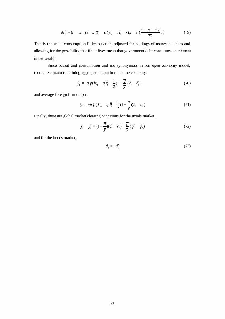
Since output and consumption and not synonymous in our open economy model,
there are equations defining aggregate output in the home economy,
*1ˆˆ ˆ ˆ ˆ( ) (1 )( )2t t t t t
gy p h P c c
yθ θ= − + + − + (70)
and average foreign firm output,
* *1ˆˆ ˆ ˆ ˆ( ) (1 )( )2t t t t t
gy p f P c c
yθ θ= − + + − + (71)
Finally, there are global market clearing conditions for the goods market,
* * *ˆ ˆ ˆ ˆ ˆ ˆ(1 )( ) ( )t t t t t t
g gy y c c g g
y y+ = − + + + (72)
and for the bonds market,
*ˆ ˆt ta a= − (73)
24
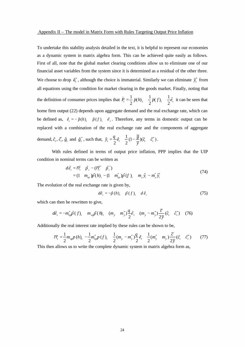
Appendix II – The model in Matrix Form with Rules Targeting Output Price Inflation
To undertake this stability analysis detailed in the text, it is helpful to represent our economies
as a dynamic system in matrix algebra form. This can be achieved quite easily as follows.
First of all, note that the global market clearing conditions allow us to eliminate one of our
financial asset variables from the system since it is determined as a residual of the other three.
We choose to drop *ˆta , although the choice is immaterial. Similarly we can eliminate *ˆty from
all equations using the condition for market clearing in the goods market. Finally, noting that
the definition of consumer prices implies that 1 1 1 ˆ( ) ( )2 2 2t t t tP p h p f ε= + +
) ) ) it can be seen that
home firm output (22) depends upon aggregate demand and the real exchange rate, which can
be defined as, ˆˆ ˆ ˆ( ) ( )t t t te p h p f ε= − + + . Therefore, any terms in domestic output can be
replaced with a combination of the real exchange rate and the components of aggregate
demand, *ˆ ˆ ˆ, ,t t tc c g and *ˆ tg , such that, *1ˆ ˆ ˆ ˆ(1 )( )
2 2t t t t
gy e c c
yθ= + − + .
With rules defined in terms of output price inflation, PPP implies that the UIP
condition in nominal terms can be written as
* *
* * *
ˆ ˆ ˆ ˆ ˆ( )
ˆ ˆ ˆ ˆ(1 ) ( ) (1 ) ( )t t t t t
op t op t y t y t
d rr rr
m h m f m y m y
ε π π
π π
= + − +
= + − + + − (74)
The evolution of the real exchange rate is given by,
ˆˆ ˆ ˆ( ) ( )t t t tde h f dπ π ε= − + + (75)
which can then be rewritten to give,
* * * *ˆ ˆ ˆ ˆ ˆ ˆ( ) ( ) ( ) ( ) ( )2 2t op t op t y y t y y t t
cde m f m h m m e m m c c
yθπ π= − + + + + − + (76)
Additionally the real interest rate implied by these rules can be shown to be,
* * * *1 1 1 1ˆ ˆ ˆ ˆ( ) ( ) ( ) ( ) ( )
2 2 2 2 2 2t op t op t y y t y y t t
crr m h m f m m e m m c c
yθπ π= − + − + + + (77)
This then allows us to write the complete dynamic system in matrix algebra form as,
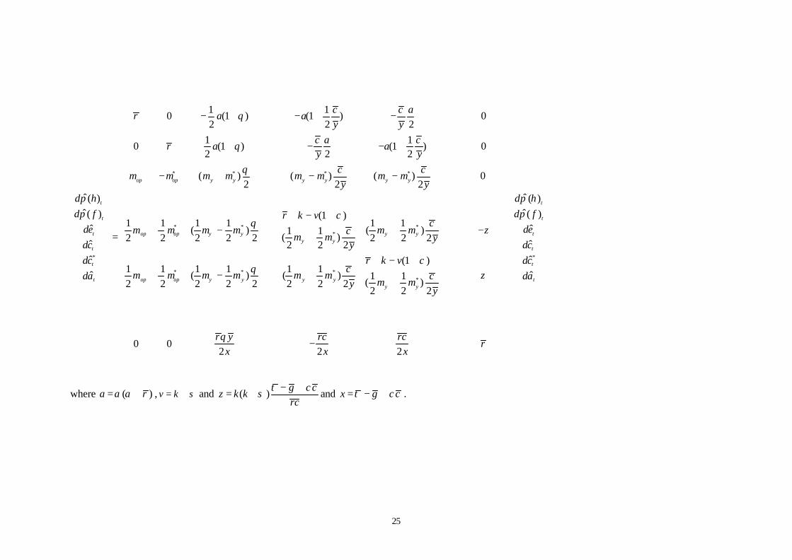
25
* * * *
* **
*
1 10 (1 ) (1 ) 0
2 2 2
1 10 (1 ) (1 ) 0
2 2 2
( ) ( ) ( ) 02 2 2
ˆ( )ˆ( ) (1 )
1 1 1 1 1ˆ ( ) (1 1( )2 2 2 2 2 2
ˆ 2 2 2ˆ
ˆ
op op y y y y y y
t
t
t op op y yy y
t
t
t
c c ar a a
y y
c a cr a a
y y
c cm m m m m m m m
y yd h
d f r k vde m m m m c
m mdc y
dc
da
θ
θ
θ
ππ χ
θ
− + − + −
+ − − +
− + − −
+ − + + −
= +
*
*
* * **
ˆ ( )ˆ( )
1 ˆ)2 2
ˆ
ˆ(1 )1 1 1 1 1 1
( ) ( ) ˆ1 1( )2 2 2 2 2 2 2 22 2 2
0 02 2 2
t
t
ty y
t
t
op op y y y y ty y
d h
d fc
dem m zy
dc
dcr k vc
m m m m m m z dacm my
y
r y rc rcr
x x x
ππ
χθ
θ
+ − + − + +
− + +
−
where ( )a rα α= + , v k σ= + and ( )g c
z k krc
τ χσ − += + and x g cτ χ= − + .

26
Appendix III – The signs of the coefficients of the determinant
( )
2 2( )[1] 2 (1 )(1 ) ( )(1 )
i
r r g g gA z z r
g y y yy
α α τθ θ σ θτ
+ −
= − + − + − − + −
6444444447444444448 (78)
In order to determine the sign of A[1] we need to know the sign of the bracketed expression,
(i). Substituting for the definition of z, and the value of the equilibrium real interest rate (50)
allows us to rewrite this as,
2
(1 )(1 ) ( )(1 )
2 ( ) (1 )(1 ) ( )
0
(1 ) (1 ) (1 ) 4 ( )( )
g gz z r
y y
gk k
y y
g g g gk k
y y y y
τθ θ σ θ
ττσ θ θ
τσ σ σ
−+ − + − − +
−+ − + + = >
−− + − − + +
(79)
Which implies that A[1]>0.
Coefficient A[3] is given by,
( )
2((1 2 )(1 ) 2 (1 ))
( )1[2]
2( )((1 2 )(1 ) )
ii
g gz
y yr rA
g g gr
y y y
θ θα ατ τ σ θ θ
+ − + − + = − −− − + − +
64444444744444448
(80)
The bracketed expression labelled (ii) can be shown to be,
2
2
(1 2 )(1 ) 2 (1 )) ( )((1 2 )(1 )
( ) (1 3 )(1 ) (1 2 )
0
(1 ) (1 ) (1 ) 4 ( )( )
g g g gz r
y y y y
g g gk k
y y y y
g g g gk k
y y y y
τθ θ σ θ θ
τ ττσ θ θ θ
τσ σ σ
−+ − + − − − + − +
−+ + − − + + + = >
−− + − − + +
(81)
by substituting for z and the equilibrium real interest rate. Here the sign of this coefficient is
positive.
Coefficient A[3] is given by,
( )
2 ( )( )[3] (1 )(1 ) ( )(1 ) 0
i
r r r g gA z z r
g y yy
α α σ τθ θ σ θ
τ
+ − −
= + − + − − + > −
6444444447444444448 (82)
Where the sign of this coefficient is determined by the same bracketed expression as in (79)
allowing us to conclude that this coefficient is also positive.
Finally, coefficient A[4] is given by,

27
( )
3
[4] (1 ) ( )
iii
g grA z r
g y yy
τσ
τ
−
= − − − −
64444744448 (83)
and the bracketed expression, (iii) can again be shown to be positive,
2
(1 ) ( )
2 ( )(1 )( )0
(1 ) (1 ) (1 ) 4 ( )( )
g gz r
y y
gk k
y y
g g g gk k
y y y y
τ σ
ττσ
τσ σ σ
−− − −
−+ −= >
−− + − − + +
(84)
28
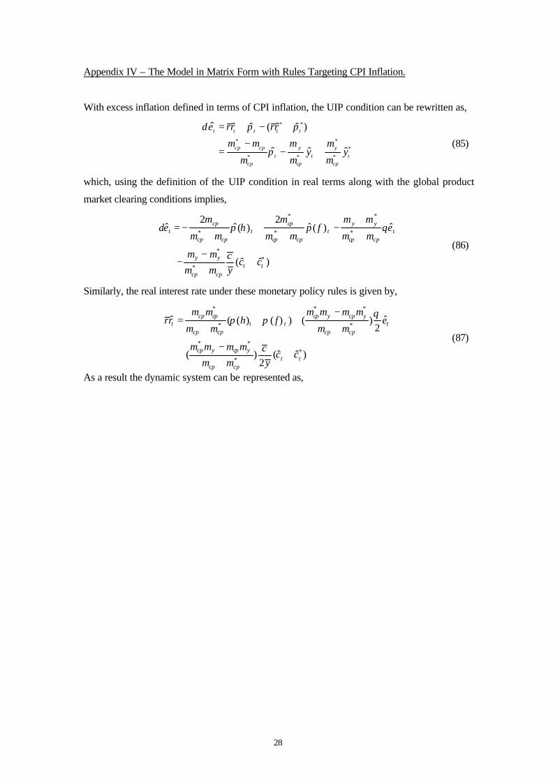
Appendix IV – The Model in Matrix Form with Rules Targeting CPI Inflation.
With excess inflation defined in terms of CPI inflation, the UIP condition can be rewritten as,
* *
* **
* * *
ˆ ˆ ˆ ˆ ˆ( )
ˆ ˆ ˆ
t t t t t
cp cp y y
t t tcp cp cp
d rr rr
m m m my y
m m m
ε π π
π
= + − +
−= − +
(85)
which, using the definition of the UIP condition in real terms along with the global product
market clearing conditions implies,
* *
* * *
**
*
2 2ˆ ˆ ˆ ˆ( ) ( )
ˆ ˆ( )
cp cp y yt t t t
cp cp cp cp cp cp
y yt t
cp cp
m m m mde h f e
m m m m m m
m m cc c
ym m
π π θ+
= − + −+ + +
−− +
+
(86)
Similarly, the real interest rate under these monetary policy rules is given by,
* * *
* *
* **
*
ˆ ˆ( ( ) ( ) ) ( )2
ˆ ˆ( ) ( )2
cp cp cp y cp yt t t t
cp cp cp cp
cp y cp yt t
cp cp
m m m m m mrr h f e
m m m m
m m m m cc c
ym m
θπ π
−= + +
+ +
−+ +
+
(87)
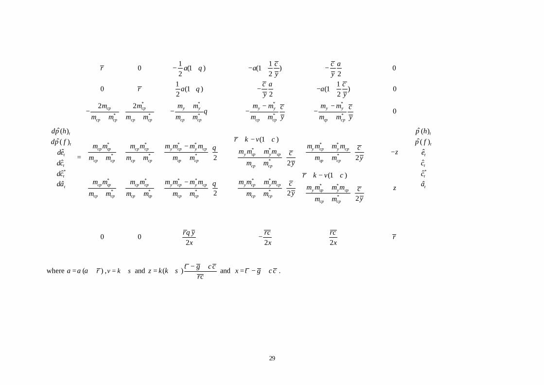
As a result the dynamic system can be represented as,
29
* * * *
* * * * *
*
*
*
1 10 (1 ) (1 ) 0
2 2 21 1
0 (1 ) (1 ) 02 2 2
2 20
ˆ( )ˆ( )
ˆ
ˆ
ˆ
ˆ
cp cp y y y y y y
cp cp cp cp cp cp cp cp cp cp
t
tcp cp cp
tcp cp
t
t
t
c c ar a a
y yc a c
r a ay y
m m m m m m m mc cy ym m m m m m m m m m
d h
d fm m m
dem m
dc
dcda
θ
θ
θ
ππ
− + − + −
+ − − +
+ − −− − − −
+ + + + +
= +
* * * * ** *
* * **
* * * * * *
* * *
(1 )
2 22
2
cp y cp y cp y cp y cpy cp y cp
cp cp cp cp cp cpcp cp
cp cp cp cp y cp y cp y cp y cp
cp cp cp cp cp cp cp c
r k vm m m m m m m m m cm m m m zc
ym m m m m mym m
m m m m m m m m m m m m
m m m m m m m m
χθ
θ
+ − + + − +
+ − + + + +
− + + + + +
*
* **
*
ˆ ( )ˆ( )
ˆ
ˆ
ˆ(1 )ˆ
22
0 02 2 2
t
t
t
t
t
ty cp y cp
pcp cp
h
f
e
c
cr k vc am m m m zcy
ym m
r y rc rcr
x x x
ππ
χ
θ
+ − + + + +
−
where ( )a rα α= + ,v k σ= + and ( )g c
z k krc
τ χσ − += + and x g cτ χ= − + .
30
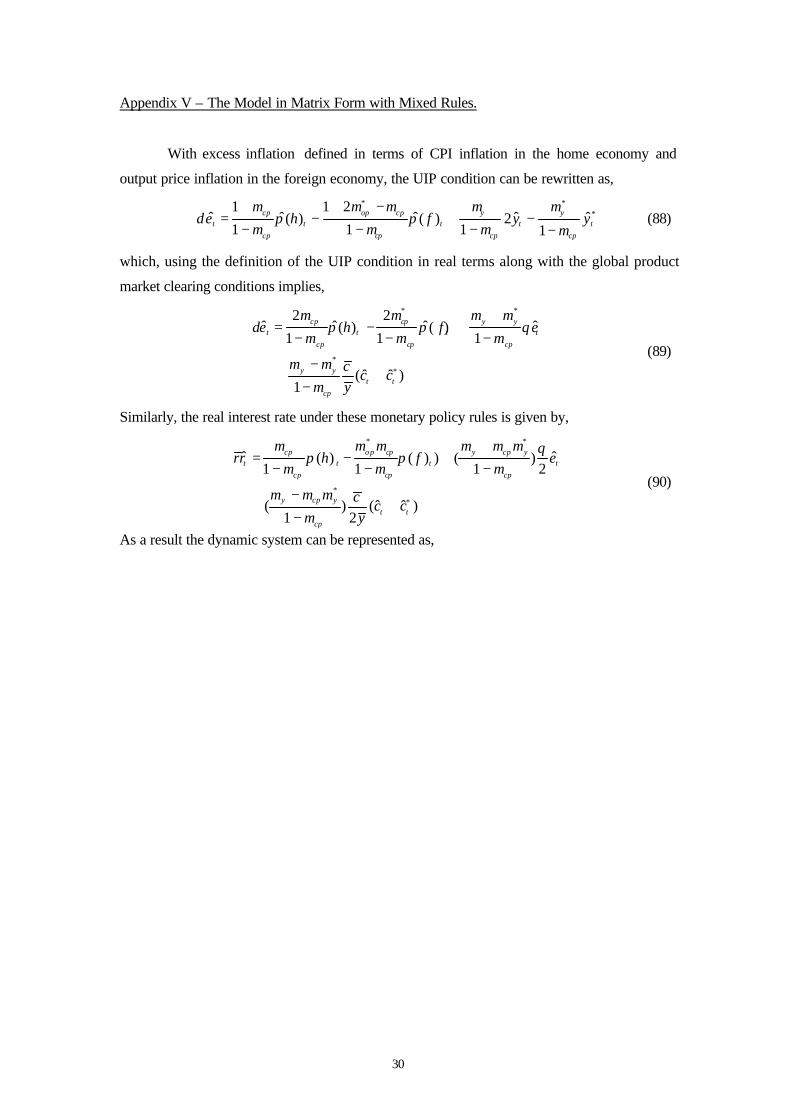
Appendix V – The Model in Matrix Form with Mixed Rules.
With excess inflation defined in terms of CPI inflation in the home economy and
output price inflation in the foreign economy, the UIP condition can be rewritten as,
* *
*1 1 2
ˆ ˆ ˆ ˆ ˆ( ) ( ) 21 1 1 1
cp op cp y yt t t t t
cp cp cp cp
m m m m md h f y y
m m m mε π π
+ + −= − + −
− − − − (88)
which, using the definition of the UIP condition in real terms along with the global product
market clearing conditions implies,
* *
*
*
2 2ˆ ˆ ˆ ˆ( ) ( )
1 1 1
ˆ ˆ( )1
cp cp y yt t t t
cp cp cp
y yt t
cp
m m m mde h f e
m m m
m m cc c
m y
π π θ+
= − +− − −
−+ +
−
(89)
Similarly, the real interest rate under these monetary policy rules is given by,
* *
*
*
ˆ ˆ( ) ( ) ) ( )1 1 1 2
ˆ ˆ( ) ( )1 2
cp op cp y cp yt t t t
cp cp cp
y cp y
t t
cp
m m m m m mrr h f e
m m m
m m m cc c
m y
θπ π
+= − +
− − −
−+ +
−
(90)
As a result the dynamic system can be represented as,

31
* * * *
* *
*
1 10 (1 ) (1 ) 0
2 2 2
1 10 (1 ) (1 ) 0
2 2 2
2 20
1 1 1 1 1
ˆ ( )ˆ( )
ˆ1 1 1
ˆ
ˆ
ˆ
cp op y y y y y y
cp cp cp cp cp
t
tcp cp op y y cp
tcp cp cp
t
t
t
c c ar a a
y y
c a cr a a
y y
m m m m m m m mc cm m m m y m y
d h
d fm m m m m m
dem m m
dc
dcda
θ
θ
θ
ππ
− + − + −
+ − − +
+ − −−
− − − − −
+ −
− − −=
**
* * **
(1 )
2 1 21 2
(1 )
1 1 1 2 1 21 2
0 02 2 2
y y cpy y cp
cpcp
cp cp op y y cp y y cpy y cp
cp cp cp cpcp
r k vm m m cm m m zc
m ym y
r k vm m m m m m m m m c
m m m zcm m m m y
m y
r y rc rcr
x x x
χθ
χθ
θ
+ − + + −
− − − − + − + +
+ − −− − − − − −
−
*
ˆ( )ˆ( )
ˆ
ˆ
ˆ
ˆ
t
t
t
t
t
t
h
f
e
c
ca
ππ
where ( )a rα α= + ,v k σ= + and ( )g c
z k krc
τ χσ − += + and x g cτ χ= − + .

32