Embed Size (px)
Citation preview

Taxation and Liquidity: Evidence from Retirement Savings
Elizabeth Chorvat†
University of Illinois
ABSTRACT
This paper tests the response of a cross section of U.S. households to a change in the price of liquidity by the 2003 Jobs and Growth Tax Relief Reconciliation Act, whether that response was tax efficient, and the distribution of that response. Empirical results based on regression analyses of Survey of Consumer Finances data between 1998 and 2010 suggest that lower, middle, and high-income households responded to the enactment of the dividend preference in a tax-efficient manner, increasing allocations to liquid accounts and away from tax-preferred retirement accounts. Notwithstanding the conventional wisdom among public economists and tax academics alike that behavioral responses to changes in the taxation of investments occur predominantly among the wealthy, the paper finds that the largest behavioral response to the 2003 dividend preference appears to have been among those households in the highest and lowest income groups, with the largest response among the lowest income households. If household income is an important determinant to the value of liquidity, we might well understand that those with the highest need for liquidity might have the largest response to a reduction in the cost of that liquidity. Curiously, while middle-income households responded to the lower cost of liquidity in a tax-efficient manner, theirs was a distinctly smaller response.
In both popular and academic discourse regarding the tax rate applicable to dividends,
the common assumption prior to, and indeed after, the passage of the Jobs and Growth Tax
Relief Reconciliation Act of 2003 (JGTRRA) was that capital gains preferences primarily
impact the wealthy, on the theory that high-income households held investment portfolios
which would be most affected by the rate cut.1 Director of the National Economic Council
Lawrence Summers predicted that reductions in taxation on returns to stock would accrue
† Elizabeth Chorvat is a Visiting Assistant Professor at the University of Illinois College of Business. The author would like to thank Omri Ben-Shahar, Charlotte Crane, Jim Hines, Will Howell, William Hubbard, Damon Jones, Brigitte Madrian, Willard Manning, Jim Sallee, and seminar participants at the University of Chicago, Cornell Law School, and the University of Michigan for their invaluable comments. Sincere appreciation is also extended to Gerhard Fries of the Federal Reserve Board and Catherine Haggerty at the National Opinion Research Center for their assistance with the data, and to the Office of Tax Policy Research at the University of Michigan for research support. 1 See Daniel Feenberg & Lawrence Summers, Who Benefits from Capital Gains Tax Reductions? in 4 TAX POLICY AND THE ECONOMY 1 (Lawrence H. Summers, ed. 1990) (explaining that “capital gains are highly concentrated among those with high incomes); Karen C. Burke & Grayson M.P. McCouch, Turning Slogans into Tax Policy, 27 VA. TAX REV. 747, 781 (2008); Paul Krugman, The Tax-Cut Con, N.Y. TIMES, Sept. 14, 2003, at 54 (asserting of the provisions of JGTRRA that “the core measures . . . benefit only the wealthy”).
TAXATION AND LIQUIDITY By Elizabeth Chorvat
Preliminary Draft; Please Do Not Cite or Quote
Comments Welcome Page 2
primarily to the benefit of high-income households, and that any behavioral response would
only reinforce that prediction.2 Interestingly, the largest behavioral changes seem to have
occurred among the poorest households, with combined incomes of less than $100,000.3
The paper presents evidence that the behavioral response to the rate change is related to
the value of liquidity. We might well imagine that the ability of lower-income households to
buy and hold stocks in liquid form – which is to say, outside of a retirement account – is all the
more related to the cost of liquidity, because the ability to sell stock investments in the event of
an unforeseen shock to the household budget is more important to these households. After all,
liquidity often matters more to the poor than to the wealthy. An exogenous shock to the
budget may be more hazardous to the integrity of a lower-income household than to the
integrity of a wealthy household.
To test the response of a cross section of U.S. households to a change in the price of
liquidity, whether that response is tax efficient, and the distribution of that response, the paper
examines changes to investment allocations between liquid and illiquid accounts. A simple
form of illiquid account is the tax-deferred retirement account, more accurately denominated as
a tax-deferred account or TDA.4 Under standard economic theory, individuals allocate their
portfolios in a tax-efficient manner between retirement accounts and fully taxable accounts
when they place a higher percentage of their highly-taxed assets in retirement accounts.5
2 Feenberg & Lawrence Summers, supra note __ at 16, 20-21. 3 See infra at Figure I Summary Statistics and note 62 and accompanying text. Benefits, of course, are a far more complicated issue, and are beyond the scope of this paper, which concerns only the behavioral response to the rate change, and whether that response was tax efficient. 4 For ease of exposition, I will refer to these TDAs as “retirement accounts,” although by this term I mean only tax-deferred retirement accounts. 5 James Poterba, Valuing Assets in Retirement Savings Accounts, NATIONAL TAX JOURNAL, 57 (2004) 489-512. Interest-bearing bonds, for example, to which ordinary rates apply, are more efficiently held in a tax-deferred account, as deferral provides the taxpayer greater value the higher the tax rate applicable to the income. For assets which are taxed at lower effective tax rates, however, the value of deferral is low. The paradigmatic example of a tax-favored asset would be land or so-called growth stocks, which do not pay
TAXATION AND LIQUIDITY By Elizabeth Chorvat
Preliminary Draft; Please Do Not Cite or Quote
Comments Welcome Page 3
Withdrawals from these accounts, however, generally result in significant penalties.6
Importantly, therefore, liquidity needs influence portfolio allocation.7 Moreover, there are
limits on amounts which can be placed in retirement accounts.8 Absent such considerations,
however, one would expect that individual or household portfolios would be allocated such
that the greater percentage of highly-taxed assets would be held in retirement accounts, being
those assets which can most benefit from deferral, while tax-favored assets would generally be
held outside of such accounts, in liquid form.9
Of course, the reality is more complicated than this simple story.10 Setting aside any
complications, we might generally expect that, if the applicable rate on dividends is reduced, it
would be less attractive than before to hold dividend-paying stocks in a retirement account, and
therefore we might expect to observe that the percentage of stock held within retirement
accounts would decrease. Similarly, we might expect that that amount of stock held within a
retirement account as compared to the total amount of stock in the portfolio – in and out of the
dividends and on which there is no current taxation. Upon disposition and realization of gain, however, these assets are taxed at comparatively favorable capital gains rates. 6 Under IRC §72(t), amounts withdrawn prior to age fifty-nine and one-half are generally subject to a penalty of ten percent while, under IRC §408, amounts withdrawn after that time are includible in taxable income. 7 Poterba et al., Asset Location for Retirement Savers, in PRIVATE PENSIONS AND PUBLIC POLICIES 290 (Gale et al., eds., 2004). 8 For example, under IRC §219, individuals under the age of fifty can contribute up to a maximum of $5,000 per year. For individuals over the age of fifty, the contribution limit is $6000. There are exceptions, for example, where an individual receives distributions from his or her 401(k), 403(b), or other pension plan and then contributes these amounts to his or her IRA within the proscribed period. Another type of tax-preferred vehicle would be insurance investments, which are subject to different limitations than TDAs, and which relate to the character of the investment. 9 Of course, the benefit of holding tax-preferred assets within tax-favored vehicles might be negligible, or potentially even negative because, upon withdrawal of these assets from the TDA, the fair market value of the assets withdrawn are subject to inclusion in taxable income and taxed at full ordinary rates. By contrast, if the asset is held for a substantial period of time with no current tax cost and, upon disposition, it will be taxed at capital gains rates, it might be more prudent to hold such an asset outside of the TDA. 10 Some comparatively high-tax assets are more liquid than those that carry a tax preference. Consider securities issued by the U.S. treasury as contrasted with gain from a wholly-owned small business. While the latter is generally more favorably taxed, the former is far more liquid such that, given the penalties for early withdrawal from tax-deferred accounts, it may make sense to hold some inherently liquid assets such as treasury securities outside of the retirement account. Moreover, the tax characteristics of the income generated by certain instruments have a direct effect on the nature of the cash flows they provide. For example, tax-exempt bonds pay a lower pre-tax rate of interest than would be the case if these bonds paid taxable interest.

TAXATION AND LIQUIDITY By Elizabeth Chorvat
Preliminary Draft; Please Do Not Cite or Quote
Comments Welcome Page 4
account, so to speak – might decrease as well.11 Under JGTRRA, dividends came to be taxed
at capital gains rates, with a rate of 15% for individuals in the highest tax brackets.12 Prior to
the change, dividends were taxed at rates applicable to ordinary income, which included a
maximum rate of thirty-five percent.13
This paper sets out to explore one simple hypothesis, which is to say, whether the
enactment of the 2003 dividend preference resulted in tax-efficient changes to portfolio
composition with respect to investors’ allocations of dividend-paying stocks and mutual funds
as between taxable (liquid) accounts and tax-deferred retirement accounts. While a significant
academic literature has investigated the effect of the 2003 tax cut on corporate behavior,14
scant attention has been directed toward the effect of a dividend tax preference on household
investment behavior in general, or on retirement savings in particular. This paper attempts to
make a modest contribution toward that end.
Empirical results based on regression analysis of SCF data between 1998 and 2010
suggest that lower, middle, and high-income households responded in a tax-efficient manner to
the enactment of the dividend preference, shifting stock holdings away from tax-preferred
11 For purposes of the analyses in the paper, I call these two variables the “within” estimator and the “in and out” estimator, meaning the proportion of stock invested within the retirement account and the proportion of stock in the retirement account as compared to all of the stock in the portfolio. 12 IRC §1(h). The preference rate legislation was passed as a temporary measure in 2003 and was extended in December 2010 through the end of 2012. 13 In 1998 and 2001 – the first and second of five iterations of the Survey of Consumer Finances examined here − the maximum rate of tax on dividends was 39.6 percent. This does not account for state taxes. In 2001, the Economic Growth and Tax Relief Reconciliation Act (EGTRRA) retroactively reduced the highest marginal tax rate on ordinary income from 39.6% to 39.1%, and provided for further reductions such that, when fully phased in, the highest marginal rate would be 35%. The highest marginal rate on ordinary income remained at 35% until the American Taxpayer Relief Act of 2012, actually passed in 2013, which increased the highest marginal rate to 39.6% for individuals with taxable income exceeding $400,000. To be more specific, JGTRRA altered the phase-in of EGTRRA, such that the highest marginal rate that applied in 2003 was 35%. 14 See, e.g. Raj Chetty & Emmanuel Saez, The Effects of the 2003 Dividend Tax Cut on Corporate Behavior: Interpreting the Evidence, 96 AM. ECON. REV. 124 (2006); Alan J. Auerbach & Kevin A. Hassett, Dividend Taxes and Firm Valuation: New Evidence, 96 AM. ECON. REV. 119 (2006); Raj Chetty & Emmanuel Saez, Dividend Taxes and Corporate Behavior: Evidence from the 2003 Dividend Tax Cut, 120 QUART. J. ECON. 792 (2006).
TAXATION AND LIQUIDITY By Elizabeth Chorvat
Preliminary Draft; Please Do Not Cite or Quote
Comments Welcome Page 5
retirement accounts and into taxable accounts. Household-level responses to the 2003 tax
reform were significant and robust to assumptions regarding normality, homoskedasticity, and
selection effects. Moreover, robustness checks using the 2007-2009 panel study indicate that
the results observed between 2001 and 2004 were the result of the enactment of the dividend
preference, and not as a consequence of the 2002 market downturn, or changes in the
composition of individuals entering or leaving the survey.
The most interesting findings were regarding the distribution of the behavioral
response to the rate change. While the response was strong among the wealthy, it was stronger
still among the relatively poorer households, with an increase in total stock holdings almost
twenty times as large as among the highest income households. Curiously, while the middle-
income households responded to the lower cost of liquidity in a tax-efficient manner, theirs
was a distinctly smaller response. We might easily imagine a story regarding the strong price
response by the lower-income households in the sample, given that the tax on dividends fell to
near zero for those in the 15-20 % bracket, and that liquidity would theoretically be of greater
value to the comparatively poorer households. The price response by the higher-income
households, whose tax rate was cut in half, is equally understandable, but it is difficult to
explain the much smaller response by those households in the middle-income brackets. Again,
although the behavioral response by the middle-income households was tax efficient, the total
stock holdings for that group actually fell over the period. Whether there were contravening
effects that occurred to dampen the response is an area for future research.
Part I of the paper discusses the value of liquidity and sets forth a simple model of
portfolio allocation given a liquidity constraint. Part II discusses the empirical methods used to
test the hypothesis, as well as the results of these tests. Part III details robustness checks to
confirm the results and differentiate the effects of the dividend tax change and other important
TAXATION AND LIQUIDITY By Elizabeth Chorvat
Preliminary Draft; Please Do Not Cite or Quote
Comments Welcome Page 6
events that occurred between 2001 and 2004. For example, there was a significant market
crash during the period. Part IV discusses the distribution of portfolio response, and Part V
concludes with a discussion of important limitations and possible extensions of the analysis.
I. THE VALUE OF LIQUIDITY
A. Prior Literature
Keynes described liquidity as the choice to hold cash when interest-bearing
instruments are available.15 An individual’s liquidity preference, according to Keynes, was a
function of his propensity to consume presently versus that part of his income which will be
reserved for future consumption.16 This liquidity preference, born of the propensity to
consume, was thus most heavily influenced by the uncertainty of bond interest prices.17
Because bond interest was “the reward for parting with liquidity,” interest rates were, in
Keynes’ view, the best measure of the liquidity preference.18
The alternative view of liquidity espoused by James Tobin explained the choice to hold
liquid assets – which he called “transactional” as opposed to “investment” balances – as a form
of insurance against discrepancies between receipts and expenditures.19 Liquidity has value for
the obvious reason that unforeseen events arise.20 We can easily see that liquidity preferences
will vary, both for reasons relating to one’s propensity to consume as well as to household
circumstances. Liquid balances provide opportunities for consumption.21 Tobin describes the
ability to hold investment balances rather than cash or cash equivalents as a luxury available to 15 JOHN MAYNARD KEYNES, THE GENERAL THEORY OF EMPLOYMENT, INTEREST AND MONEY 169 (1936). 16 Id. at 168-69. 17 Id. at 170. 18 Id. at 169-73. 19 James Tobin, Liquidity Preference as Behavior Towards Risk 25 Rev. Econ. Studies 65 (1958) (explaining that preference for liquidity relates to risk aversion). See generally R.L. Crouch, Tobin vs. Keynes on Liquidity Preference, 53 REV. ECON. & STAT. 368 (1971). 20 Id. 21 Listokin describes cash as providing a transaction function, “enabling investors to consume quickly and easily.” See Listokin, supra note 18, at 1685.

TAXATION AND LIQUIDITY By Elizabeth Chorvat
Preliminary Draft; Please Do Not Cite or Quote
Comments Welcome Page 7
those with sufficiently large portfolios.22 These are the wealthier households, for whom
interest is the reward for the lack of liquidity that they can well afford. On the other hand,
among those with lower incomes, random shocks to the household budget can overwhelm
current resources. As a result, liquidity constraints on lower income households have
significant effects on their savings and consumption.23 Moreover, these constraints often have
significant effects on welfare.24 In fact, the literature is well settled that liquidity constraints on
households with lower incomes have a larger effect on their behavior than households with
higher incomes.25 Consequently, one can easily surmise that a significant relaxation of
liquidity constraints would have a significant positive value to the lower-income households so
constrained. If household income is an important determinant to the value of liquidity, we
might then well understand that those with the highest need for liquidity might have the largest
response to a reduction in the cost of that liquidity. More specifically, if the subjective value
of liquidity is driving those portfolios adjustments that we observe, we might expect to see that
lower household incomes value liquidity more, and hence exhibit a larger behavioral response
to the rate change.
B. A Simple Model of Portfolio Allocation
We have from Keynes and Tobin that the choice between liquid and illiquid assets is
driven by both propensity to consume and uncertainty. We might well imagine that the
liquidity preference is also impacted by taxation, because taxation alters the cost of liquidity.26
22 Tobin, supra note 19, at 66. 23 Angus Deaton, Saving and Liquidity Constraints, 59 ECONOMETRICA 1221 (1991) 24 Tullio Japelli & Marco Pagano, The Welfare Effects of Liquidity Constraints, 51 OXFORD ECON. PAPERS 410 (1999). 25 R. Glenn Hubbard & Kenneth Judd, Liquidity Constraints, Fiscal Policy and Consumption, 1 BROOKINGS PAPERS ON ECONOMIC ACTIVITY 1 (1986). 26 Of course, taxation may also alter the income associated with illiquid assets, but that is beyond the scope of this paper. See Listokin, supra note 18, at 1686-88 (describing the impact of asymmetric taxation on the
TAXATION AND LIQUIDITY By Elizabeth Chorvat
Preliminary Draft; Please Do Not Cite or Quote
Comments Welcome Page 8
A number of recent studies have analyzed the effects of taxation on portfolio choice.27 These
studies have generally found that households make decisions that can at least roughly be
thought as rational with respect to tax rates.28 That is, as the marginal tax rate on a certain type
of income increases, a taxpayer is less likely to invest in that type of asset. Furthermore, more
highly taxed assets are more likely to be held in tax-deferred accounts, thus reducing the tax
rate on the income from such an asset.29
Taking together the value of liquidity discussed in the prior section with the models of
portfolio selection just discussed, we can derive a simple model of the effect of reducing the
taxation of dividends on household portfolio choice. The model of portfolio choice discussed
in this section is given in order to motivate the empirical discussion in the rest of the paper.
We might thus expect that individuals preferentially allocate to their tax-deferred
accounts those assets that are comparatively highly taxed and that, all else being equal, if an
asset becomes more favorably taxed, individuals will reallocate some of these investments
away from tax-preferred but less liquid accounts in favor of fully-taxable accounts. We can
write a very simple model to illustrate this concept.
If we consider that an individual will hold an exogenously-determined amount of stock
, where the tax rate is , the return on the stock is , and the proportion of stock held
outside of the tax-deferred account is , and the value increase due to greater liquidity from
choice between holding in liquid or illiquid form as a distortion of the interest rate earned on investment balances). 27 James Poterba & Andrew Samwick, Taxation and Household Portfolio Composition: US Evidence from the 1980s and 1990s, 87 J. PUBLIC ECON. 5 (2003). See also Daniel Bergstresser & James Poterba, Asset Allocation and Asset Location: Household Evidence from the Survey of Consumer Finances, 88 J. PUBLIC ECON. 1893 (2004). 28 For example, Poterba and Samwick found that the likelihood of owning tax-favored assets such as tax exempt bonds is highly correlated with the marginal tax rate on ordinary income for the household. 29 Bergstresser and Poterba, supra, note 27.
S � r
a

TAXATION AND LIQUIDITY By Elizabeth Chorvat
Preliminary Draft; Please Do Not Cite or Quote
Comments Welcome Page 9
not being held in a tax-deferred account (“liquidity value”) is the function , where
, , then we can set up the maximization problem in the following manner.30
(1)
The first order condition is then:
, (2)
which gives us that:
. (3)
As decreases, the denominator increases, such that the fraction decreases. Because
is concave, as the derivative decreases, the argument of the function – the amount of stock
allocated to the taxable account – must increase.31 In other words, a larger percentage within
the stock portfolio must be allocated to taxable accounts rather than held in the TDA. Of
course, reducing the tax rate might also increase the optimal proportion of the portfolio
allocated to stock and, indeed, the allocation between tax-deferred and taxable accounts may
also affect the optimal level of stock. Adding such considerations will only complicate the
model, however. It will not change the basic result that, where the tax value of deferral
decreases, but the liquidity value does not, then a larger portion of stock should be held outside
of the tax-deferred account.
We might also expect that the proportion of assets held as stock within the tax-deferred
accounts would decrease as more stock is held outside of the TDA. As the amount of stock
held within the TDA decreases, we would then expect that other assets would make up a larger 30 I am simplifying somewhat here by treating the returns in the tax-deferred account as if they are in fact tax free. We could, alternatively, treat r as the after-tax rate of investments in the tax-deferred account and as the additional tax rate they face in the fully taxable accounts. 31 Note that the argument of the function, which is to say, , represents the amount of stock held outside the tax-deferred account. For a proof that a, the proportion of stock allocated to taxable accounts, must increase as decreases, see Appendix C.
maxaL aS 1+ 1��( )r( )�� ��+ 1�a( )S 1+ r( )
� �� � � �� �� �1
1 11 1S r
L aS rS r
��
�� �� � � � �
�
�

TAXATION AND LIQUIDITY By Elizabeth Chorvat
Preliminary Draft; Please Do Not Cite or Quote
Comments Welcome Page 10
percentage of the account. Returning to the model, as a increases, the increase will be
reflected by associated changes in both the numerator and denominator of equation (3). In
sum, then, we would expect that the proportion of TDA held as stock, as compared to other
assets, would decrease.
A significant assumption of this analysis is that the other characteristics of equity
remain the same. For example, if a large number of companies did not pay dividends before
this change, and began to pay dividends following the change in the tax rules, then it might be
the case that equities would become less tax favored, which would alter the underlying
allocation.32 If this occurred, it would be difficult to make any predictions without knowing
more about the changes to dividend policies, the tax situations of individual investors, as well
as their liquidity preferences. Noting, then, that this model may appear to be too simplistic to
fully describe behavior under every eventuality, we will nonetheless proceed to test whether it
accurately predicted investor behavior following the 2003 Act.
To recapitulate, the basic intuition is that, if the deferral value of holding stock in a
TDA is decreased, holding liquidity value constant, we would expect less to be held within the
account. We would then expect the proportion of stock within the TDA as compared to other
assets in that account to decrease. Moreover, we would expect the proportion of the investor’s
portfolio of stock in the TDA as compared to the proportion outside the TDA would decrease.
II. EMPIRICAL TESTS
A. Data
In order to examine investor responses to the enactment of the 2003 dividend
preference, I analyze data from four successive reports from the Survey of Consumer Finances: 32 The stock of companies which pay out dividends is more highly taxed than the stock of companies which do not, since every year dividends are taxed, as compared with capital gains being taxed at some point in the future.

TAXATION AND LIQUIDITY By Elizabeth Chorvat
Preliminary Draft; Please Do Not Cite or Quote
Comments Welcome Page 11
those surveys for 1998 and 2001, which report data for years prior to the tax law change, and
those surveys for 2004, 2007, and 2010, which report data for years to which the change in the
tax code applied.33 I utilize data from these sources to examine whether there were any
observable shifts in the patterns of asset allocation within tax-deferred accounts or in the
pattern of allocating stock holdings both within and without TDAs.
To better understand some of the basic context for the analysis presented, we might
examine the basic statistics.
Figure I. Summary Statistics
Total observations: Total with positive TDA balances: Average Income 1998-2001: Average Income 2004-2010: Median Income 1998-2001: Median Income 2004-2010: Median Age 1998-2001: Median Age 2004-2010: Average IRA balances 1998-2001: Average IRA balances 2004-2010: Average stock holding in TDA 1998-2001: Average stock holdings in TDA 2004-2010: [To be included: Average Holdings in TDA by income] Average proportion of TDA held in stock 1998-2001: Average proportion of TDA held in stock 2004-2010:
33 The Federal Reserve Board’s Survey of Consumer Finances is “a triennial survey of the balance sheet, pension, income, and other demographic characteristics of U.S. families.” See http://www. Federal reserve.gov/pubs/oss/oss2/scf index.html (last visited April 17, 2011). Note that we might not expect to observe a significant change in behavior reflected in the SCF for 2004 as a direct result of legislative changes in 2003, because the change would have occurred in mid-2003 (to affect January 1, 2004 and beyond) and the SCF for 2004 could reflect data from as early as statements from the last quarter of 2003.

TAXATION AND LIQUIDITY By Elizabeth Chorvat
Preliminary Draft; Please Do Not Cite or Quote
Comments Welcome Page 12
Average proportion of total stock held in TDA 1998-2001: Average proportion of stock held in TDA 2004-2010: [To be included: Average Proportions in TDA by income]
Average Stock holding outside of TDA by Income: Income level < $100,000 $100,000-200,000 > $200,000 1998-2001 36,955 280,247 6,142,554 2004-2010 78,762 128,236 6,578,348
Total TDA balances by Income: Income level < $100,000 $100,000-200,000 >$200,000 1998-2001 17,420 119,538 440,536 2004-2010 24,484 101,841 589,567
From the above statistics, we can see that survey respondents are little older than the
U.S. population, and perhaps a little wealthier on average as well.34 However, they do not
appear to so different from the population to undermine our inferences for the purposes
external validity.
We might note that it was among the lower-income individuals that we see the largest
increase in stock held outside of the account. By contrast, we see that the middle-income
households actually saw a reduction in the amount of stock held outside of the TDA. We will
address this in greater detail infra in Section IV, DISTRIBUTION OF PORTFOLIO RESPONSE.
We see a similar pattern emerging for total retirement account balances. The higher
and the lower-income groups both exhibited higher total balances following imposition of the
dividend rate preference, while the middle-income households saw a reduction in total TDA
balances after the tax changes.
34 The US census lists the median age of the US population in 2010 as 37, and the median household income as 49,277. UNITED STATES CENSUS BUREAU, HISTORICAL TABLES, TABLE H-8.

TAXATION AND LIQUIDITY By Elizabeth Chorvat
Preliminary Draft; Please Do Not Cite or Quote
Comments Welcome Page 13
To calculate a rough elasticity of response to the dividend rate cut, we use can use the
standard elasticity formula of differences in demand divided by differences in the tax rates.35
For the proportion of the TDA held in stock, we find that the SCF respondents seemed to have
exhibited an elasticity of for the within estimator while, for the proportion of stock held
in the TDA versus outside of it, they seem to have exhibited an elasticity of .36 These
are broadly consistent with the CBO’s estimate of the long-run elasticity of capital investment
to tax of .37
B. Estimating Stock Proportions
Unfortunately, the Surveys for years prior to the 2004 report did not question
respondents explicitly about the specific percentage of stock (as opposed to other assets) held
in his or her IRA or other tax-deferred accounts. This might appear to be a stumbling block in
our quest to use the data to test our hypothesis. Fortunately, a method developed by
Bergstresser and Poterba allows us to estimate the proportion of tax-deferred accounts which
are held in stock and, from this, we can estimate the amount of stock held in TDAs by our
respondents.38 More specifically, the Bergstresser and Poterba methodology is to use the
results of a question in which the Survey asked generally how the TDA was allocated, in
addition to asking how much was invested in the TDAs owned by the respondent as well as
35 That is we calculate .
36 In calculating the elasticities above, I use the tax rates for those households in the highest income brackets, because capital is earned largely by this group. See Thomas L. Hungerford, Changes in the Distribution of Income Among Tax Filers between 1996 and 2006: The Role of Labor Income, CAPITAL INCOME AND TAX POLICY, CONGRESSIONAL RESEARCH SERVICE (2011). 37 Tim Dowd, Robert McClelland & Athiphat Mathitacharoen, New Evidence on the Tax Elasticity of Capital Gains, JCX-56-12 (2012). 38 Daniel Bergstresser & James Poterba, Asset Allocation and Asset Location: Household Evidence from the Survey of Consumer Finances, 88 J. PUBLIC ECON. 1893 (2004).
TAXATION AND LIQUIDITY By Elizabeth Chorvat
Preliminary Draft; Please Do Not Cite or Quote
Comments Welcome Page 14
other members of the respondent’s household. This question, or an essentially identical
question, has been employed for many years in the SCF. Fortunately, these questions were
asked in every year in which we are utilizing the Bergstresser and Poterba variable, the SCF
not having asked the explicit allocation question in the years prior to 2004.39 To be precise, the
relevant question posed by the Survey in each of the four years under examination was:
How is the money in (all) your family's IRA and Keogh account(s) invested? Is most of it in CDs or other bank accounts, most of it in stocks, most of it in bonds or similar assets, or what? Note that this question does not elicit a specific percentage of the TDA invested in
each of these asset categories. Rather, it merely asks respondents to give a gross generalization
of the how the TDAs are invested. Possible answers are “all” or “mostly” to stock or bonds, to
CDs, or to other specific asset classes. Bergstresser and Poterba utilized the responses to this
question by making the simplifying assumption that, where individuals stated that the TDA
was “all or mostly” invested in stock, then the entire account was allocated to stock. Where
the respondents indicated that the TDA was “split” between stocks and a single other asset
class, then half of that person’s TDA was assumed to be designated as held in stock. While not
stated explicitly in the article, it would appear that, where the respondent stated that his or her
investments were “split” between stocks, bonds, and CDs, then one-third of the TD was
assumed to be allocated to stock. Because essentially the same question was asked in the 2004
and 2007 SCFs, we can utilize a similar methodology to estimate the amount of stock held in
tax-deferred accounts at that time.40
39 Because we are able to confirm the accuracy of the Bergstresser and Poterba variable as an estimator for the value of stock held within the TDA, we can proceed to utilize the variable for all four years under analysis. 40 As will be discussed later in the paper, it turns out that the methodology employed by Bergstresser and Poterba predicts rather well the proportion of the respondents’ TDAs allocated to stock. Taking advantage of an additional question which was added to the Survey beginning in 2004, as well as information provided by the Federal Reserve, we will be able to see that the Bergstresser and Poterba methodology actually predicts

TAXATION AND LIQUIDITY By Elizabeth Chorvat
Preliminary Draft; Please Do Not Cite or Quote
Comments Welcome Page 15
While the Bergstresser and Poterba variable provides important information, we must
pair this allocation estimate with the amount invested within a given respondent’s TDA(s) in
order to determine how much stock was held in that account(s), as well as to determine the
average proportion of stock within the TDA(s) as compared to the total value invested in the
TDA(s). Fortunately, the Survey asks individuals to provide the value of their tax-deferred
accounts, so we are able to determine these amounts.41
In addition to testing the change in the proportion of stock within the TDA, we could
also test whether the proportion of stock held inside the IRA(s) versus that held inside plus
outside the IRA(s) changed as a result of change in the tax law. For this, we would also need
to know the value of stock held outside of the IRA. Luckily, the SCF inquires after the value
of stock and mutual funds held by individuals not in TDAs or other tax-preferred vehicles.
To summarize, then, this paper utilizes data explicitly measured by the SCF, in
addition to a methodology employed by Bergstresser and Poterba, in order to analyze whether
households which have financial assets in both taxable and tax-deferred accounts held
portfolios that were tax efficient.42 This extends the Bergstresser and Poterba analysis to
investigate whether changes to the tax law in 2003 altered individual investors’ allocations of
stocks and mutual funds that pay dividends, as between taxable and tax-favored accounts.
More specifically, for example, this paper examines whether there was a change in portfolios
with respect to the percentage of stocks versus bonds which, because equities became
relatively more tax favored, should have been shifted out of tax-favored vehicles such as
retirement accounts. quite well the respondents’ own estimates of the percentage of stock within their TDAs. See Part III relating to discussions with Gerhard Fries of the Federal Reserve Board. 41 Please refer to Appendix A for the wording of the questions. 42 Bergstresser & Poterba, supra note 31. The authors found that approximately two thirds of households with financial assets in both taxable and tax-deferred accounts held portfolios that are tax efficient, and that most of the other third could have reduced their taxes by relocating heavily taxed fixed income assets to their tax-deferred account.

TAXATION AND LIQUIDITY By Elizabeth Chorvat
Preliminary Draft; Please Do Not Cite or Quote
Comments Welcome Page 16
Recall that, in order to pursue this investigation, we need to know or be able to
estimate the amount of stock held in TDAs, the total size of these accounts, as well as the total
amount of stock held outside of such deferral vehicles. As discussed above, the question
regarding the precise level of stocks within the TDA is only included in the SCF questionnaire
for years beginning with 2004. Because I utilize the Bergstresser and Poterba methodology we
might then, as an initial matter, first examine whether the Bergstresser and Poterba formulation
is a good estimator of the amount invested in stock in the tax-deferred account. Toward that
end, I compared the Bergstresser and Poterba estimator for the years 2004 and 2007, with the
more precise estimate we can obtain from the SCF data for those same years.
For the 2004 survey, we find that the Bergstresser and Poterba variable gives us an
estimate of an average value of $41,841.32 of stock contained in the TDAs of survey
participants. By comparison, the more precise estimate for stock within the TDAs provided by
the explicit question introduced in the 2004 survey, and included since that time, gives us an
estimate of $42,156.86. This is a difference of $315.54, which implies the Bergstresser and
Poterba estimator is not a bad estimator for the amount of stock held in TDAs. Making the
same comparison for the 2007 survey yields a Bergstresser and Poterba estimator of
$46,156.31 for stock within the TDA. What we might denominate the more precise or “direct”
estimator introduced in 2004 yields an estimate of $47,352.36. Again, the Bergstresser and
Poterba estimator proves to be a good, although not perfect, estimator.
Note that we are not necessarily interested in estimating the absolute level, but rather
we are interested in performing statistical inference based on changes to these levels. We can
see that, for the more precise or direct estimate, we find an average increase of stock in the
TDA between 2004 and 2007 of . By comparison, for
the Bergstresser and Poterba estimator, we observed a growth of

TAXATION AND LIQUIDITY By Elizabeth Chorvat
Preliminary Draft; Please Do Not Cite or Quote
Comments Welcome Page 17
. Again, the estimator performs fairly well. It is in the correct direction and with
about the correct magnitude.43 Obviously the comparison is not perfect, but perhaps much
better than one might initially predict, given the seeming ad hoc nature of the Bergresster and
Poterba estimator. We might also note that this estimator is not the result of data mining the
2004 and 2007 data, but rather was hypothesized before the data were collected.44 Therefore,
it seems reasonable to say that the Bergstresser and Poterba estimator does give some
indication of the change in the amount of stock within the tax-deferred accounts. If we find
highly significant results, this would indicate that we would have likely found similar results if
the more precise estimator had been available in earlier iterations of the Survey.
C. Estimating Control Variables
Having now a principled estimator that we can use to compare portfolio allocations
both before and after the 2003 dividend tax change, we now can proceed to test whether
investors undertook the changes in portfolio allocations that we might expect to see if they are
making tax efficient decisions. Prior to describing the specifications we will test, we might
first note that we should control for a number of factors which might confound the effects we
seek to isolate. For example, it is common that investors are advised to shift their portfolios
away from stock as they near retirement. Moreover, as one nears retirement, the liquidity
restrictions that result from the early withdrawal penalty become less significant. As a result,
if the subject population ages, we would expect that the portfolio allocations of the investors
43 Note that this slight increase in the average value of stock within TDAs between 2004 and 2007 is reflected in Figure 2 at page 16, infra. Recall that both of these years are after the enactment of the new dividend tax regime. If we were to compare the average amount of stock in tax-deferred accounts before the change (which is to say, for Survey years 1998 and 2001) to the amount after the change (years 2004 and 2007), we would expect to find that the total amount of stock is less the years after the change as compared to the years before the change. 44 Recall that Bergstresser & Poterba was published in 2004.
TAXATION AND LIQUIDITY By Elizabeth Chorvat
Preliminary Draft; Please Do Not Cite or Quote
Comments Welcome Page 18
should change. To account for this possibility, the specifications include controls for both age
and age squared.
Another concern for which we must account would be the notion that risk aversion is
to some degree a function of wealth. In order to account for this effect, the specifications
below include the natural logarithm on income as a control.
Next, we might naturally imagine that market fluctuations are something for which we
should account. The value of the S&P 500 (a reasonable index for valuing stock and mutual
funds in TDAs) was 1,211 on July 1, 2001. On July 1, 2004, the index reported a value of
1,128, which is rather similar. By contrast, on July 1, 2007, the value of the S&P 500 was
1519.43 and, on July 1, 1998, it was reported as 1236.72. We might imagine that the closing
values on these dates would be reasonably illustrative of stock markets for the relevant years,
being at the midpoint of each year, and thus might well represent the market value at the time
when the average respondent could be providing data to the Survey.
Of particular concern for this analysis, however, is the fact that the value of the S&P
500 on January 1, 2001 was 1,366, and value in January 1, 2004 was 1,111. In other words,
there was a reduction in the market value of large-cap stocks of about 19% between these two
dates. If survey respondents were referencing old quarterly statements, as opposed the values
which they could obtain online, it is possible that a change in market value might explain most
or even all of the differences that we observe. The plausibility of this explanation, however,
would depend on when respondents were surveyed.
Unfortunately, in the public data set, we are not provided the dates on which
respondents were surveyed, nor do we know how they obtained the values reported for the
total amounts in their retirement accounts. So, while we cannot know with any degree of
certainty, it may be the case that, having made an allocation within their tax-deferred accounts,

TAXATION AND LIQUIDITY By Elizabeth Chorvat
Preliminary Draft; Please Do Not Cite or Quote
Comments Welcome Page 19
respondents did not rebalance, either for market changes or for changes in the tax law. In other
words, the sharp decline in stock prices between 2001 and 2004 may have caused the reduction
in the proportion of the TDAs allocated to stock evident in Figure 1, infra at page 16. Thus,
inertia, together with a drop in the stock market, could have combined to cause a reduction in
the proportion of the IRA accounts allocated to stock. Because market fluctuations affect the
stock held outside deferral accounts in the same manner as inside, we might expect, however,
little difference in the proportion of stock held within TDAs versus that held outside of these
accounts.
D. Specifications and Empirical Findings
We consider two major tests of the hypothesis that, in a tax-efficient response to the
2003 change to the taxation of dividends that made allocations of stock to tax-deferred
accounts less valuable, investors reduced these allocations. In the first specification, we test
the proportion of tax-deferred accounts allocated to stock before and after the 2003 legislation.
The second tests the effect of the tax change on the proportion of stock held within tax-
deferred accounts as compared to outside of these accounts. I believe that this second test is
important because we might observe a drop in the proportion of TDAs invested in stock simply
because the market declined over the period. As it happens, the empirical results suggest that
the S&P 500 does not affect investor allocations ‒ a result that may run counter to one’s initial
intuition.
Specification (1)
Specification (2)

TAXATION AND LIQUIDITY By Elizabeth Chorvat
Preliminary Draft; Please Do Not Cite or Quote
Comments Welcome Page 20
Results from regressions performed according to these specifications are presented below.
Table 1. OLS Specifications
____________________________________________________________________________________________________________
TDA Percent in Stock
(1)
Percent Stock in TDA (2)
Dividend Tax -0.137***
(0.002) -0.127***
(0.003) Ln Income 0.036***
(5.87e-04) -0.008***
(6.00e-04) S& P July 1 3.09e-05
(4.63e-06) -6.26e-06 (6.02e-06)
N=24,16645
*** p<0.01, ** p<0.05, * p<0.1 ______________________________________________________________________________________ Notes: standard errors in parentheses. Also included are regressors for age, age squared, and average S&P. Source: Author’s calculations using SCF data.
Here we find several interesting results. First, we would have predicted that the level
of the S&P 500 would have been correlated with the proportion of tax-deferred accounts held
in stock. Many mutual funds are designed to track the S&P. We know from the results of
specification (1) that the index is not correlated with movements within the deferral accounts.
From the results of specifications (2), we can conclude that the index is not correlated with
movements outside of these accounts. This result may relate to the fact that we only consider
four time periods. Of course, if survey respondents actually rebalance their portfolios within
their deferral accounts to maintain their preferred allocations, this is precisely what we would
expect to see. We might have expected that the S&P 500 would have a higher correlation with
45 The SCF reports imputed values for missing data such that the uncorrected number of observations is five times the actual number of observations. The number reported in all tables in this paper is the actual number of observations. Left uncorrected, the imputation process would result in incorrect standard errors. In order to address this issue, I utilized the repeated-imputation inference method. See DONALD B. RUBIN, MULTIPLE IMPUTATION FOR NONRESPONSE IN SURVEYS (1987).

TAXATION AND LIQUIDITY By Elizabeth Chorvat
Preliminary Draft; Please Do Not Cite or Quote
Comments Welcome Page 21
those assets held outside the tax-deferred accounts, since it is not costless to rebalance outside
of these account.46
While we see that there is a significant decrease in both the proportion of stock in tax-
deferred accounts both within in the deferral acounts and as compared to stock held outside of
the TDAs as well, we cannot be sure that these changes are the result of the change in the
taxation of dividends. Unfortunately, all of the years associated with the dividend tax
preference are after 2003, and all of the years that tax dividends at ordinary rates are before
2003. Since all of the years with the dividend preference are after the tax change, anything that
changed between 2001 and 2004 and continues will be confounded with the dividend tax
change. Therefore, if there was a secular trend resulting in allocations to stock in tax-deferred
accounts, we would still observe the same result. If we look at a time series of the proportion
of the tax-deferred account invested in stock − given in Figure 2 below − we see that there
does not apear to be a secular trend resulting in a lower proportion of the TDA being invested
in stock. While this evidence is not dispositive, it is indicative of the absence of such a trend.
Figure 2.
46 If it is costly to trade, inertia should play a larger role. Because trades have a tax cost outside of tax-deferred accounts, it would be more costly for investors to rebalance their portfolios outside the TDA than within these accounts. Therefore, we would expect to find more correlation outside of the deferral accounts. I am not entirely confident of this reasoning, but it would explain the observed results.
0
0.05
0.1
0.15
0.2
0.25
0.3
1998 2001 2004 2007 2010
Proportion of TDA in Stock "within"
Proportion of TDA in Stock

TAXATION AND LIQUIDITY By Elizabeth Chorvat
Preliminary Draft; Please Do Not Cite or Quote
Comments Welcome Page 22
We see a slightly different result if we look at a time series of the proportion of stock
held within the tax-deferred account as compared to the total amount of stock in the portfolio.
Figure 3.
While the time series for the allocation within the tax-deferred accounts as shown in
the “Proportion of TDA in Stock” at Figure 2 appears to provide good evidence for the
proposition that something occurring between 2001 and 2004 had a significant impact on stock
allocation within the portfolio, this is less clear in the “Proportion of Stock in TDA” time series
at Figure 3. While is it true that the proportion of stock held within the TDAs is lower for both
years following the dividend tax change than was the case for the both of the years before the
tax change, the most significant decrease in the portion of stock held inside tax-deferred
accounts appears to have occurred between 2004 and 2007. The reason for this is not entirely
clear, although we might reasonably imagine that it takes time to accumulate a greater
proportion of stock outside of the TDAs, or that taxpayers were more willing to accumulate
stock in their taxable accounts after it appeared more certain that the dividend preference
would remain in place for some period of time.
0 0.05
0.1 0.15
0.2 0.25
0.3 0.35
1998 2001 2004 2007 2010
Proportion of Stock in TDA "in and out"
Proportion of Stock in TDA
TAXATION AND LIQUIDITY By Elizabeth Chorvat
Preliminary Draft; Please Do Not Cite or Quote
Comments Welcome Page 23
In the next section, I utilize standard robustness checks to address the potential issue of
the secular trend, as well as to address the concerns typically associated with cross sectional
data, such as individuals entering or leaving the survey or possible changes to the type of
individual willing to be surveyed (selection effects). Moreover, our observations are
necessarily right censored, since we are dealing with proportions. Additionally, there is of
necessity a lower bound of zero for these proportions, because individuals are precluded under
the applicable regulations from holding naked short positions within a tax-deferred account.
This means that the taxpayer’s net investment in all stocks within the TDA cannot be below
zero, when short and long positions are considered together. Because the data are thus
inherently double censored, it is important to confirm our results from OLS with regression
analyses that take this censoring into account.
III. ROBUSTNESS CHECKS
In addition to the concern common to all such studies that the results which we observe
are the consequence of a secular trend, rather than the change in the law, there are issues with
cross sectional data that should be addressed with regarding individuals entering and leaving
the study, as well as possible changes to the type of individual willing to be surveyed. In
performing robustness checks to address these issues, and to ascertain whether the results
obtained are sensitive to modeling changes, I have employed (i) a synthetic panel and (ii) an
analysis of the recently released “short panel” for 2007-2009. Moreover, in order to address
the possibility for confounded results on account of censored data, I utilize Tobit, censored
least absolute deviation (CLAD), symmetrically-trimmed least squares (STLS), and censored
conditional mean analyses to confirm the results originally obtained using OLS.
A. Synthetic Panel
TAXATION AND LIQUIDITY By Elizabeth Chorvat
Preliminary Draft; Please Do Not Cite or Quote
Comments Welcome Page 24
Panel data allows us to track individuals ensuring that the differences that we observe
are differences in the control variables, rather than different people entering the observational
data. Here, we want to ensure that we are observing changes in the investment behavior of
individuals over time, and not the investment behavior of different individuals. This is difficult
to do with cross-sectional data, since there are always new individuals entering the data over
time. Synthetic panel data is intended to approximate panel data. Instead of tracking
individuals over time, we track the average of the cohort over time, . In particular, we
group individuals into cohorts, according to characteristics that do not change over time – or
change in a predictable fashion – and observe the differences in the averages over time, which
becomes almost like observing a single person over time.
Following Deaton (1985), we employ synthetic cohorts in the following model:
′
where and , The cohorts were formulated based on date of birth
within three-year periods, observed across the period from 1998 to 2007. Although we lose
some “coverage” at the ends, primarily abound eighteen years of age and ninety-five years of
age, we have sufficient data with the SCF, primarily between the ages of twenty-five to eighty-
five. A synthetic panel may help to answer the question as to whether individuals altered their
investment behavior for reasons other than the tax change incorporating a rate preference for
dividends such as, for example, a secular decrease in stock or a secular increase in retirement
savings vehicles other than stock. Following Devereaux (2006), and grouping by three-year
cohorts (and a bit longer in the tails), we have only about 20-25 cells into which we can place
the respondents’ 21,525 observations. For the synthetic panel, we can utilize the fixed effects
estimator and the random effects estimator. Note that the Tobit is not useful here because, with

TAXATION AND LIQUIDITY By Elizabeth Chorvat
Preliminary Draft; Please Do Not Cite or Quote
Comments Welcome Page 25
a synthetic panel, we track the average of a cohort over time, so there are no zero observations,
and no censored data. We find the results to be somewhat similar for the two specifications.
Table 2. Fixed Effect Specifications on Synthetic Panel
____________________________________________________________________________________________________________
TDA Percent in Stocks
(within) Percent Stock in TDA
(in and out)
Dividend Tax 0.0020 (0.012)
-0.088*** (0.024)
Ln Income 0.0068 (0.011)
-0.026* (0.023)
S&P July 1 0.000*** (0.000)
-0.001*** (0.000)
Observations = 21,525 Groups = 21
*** p<0.01, ** p<0.05, * p<0.1
________________________________________________________________________ Notes: standard errors in parentheses. Also included are regressors for age, age squared, and average S&P. Source: Author’s calculations using SCF data.
Note that all of our variables, including the tax dummy, are time based, so fixed effects
works well here. In this case we see that for the proportion of stock held inside the retirement
account as a proportion of the portfolio as a whole, the coefficient on the dummy variable for the
tax change has the predicted sign. It does not have the predicted sign, however, for that proportion
of the retirement account which is held in stock. We might note that that the coefficient is not
statistically significant. Therefore, the fixed effects specification on the synthetic panel is
inconclusive with regard to the effect of the dividend tax change on the allocation of stock within
the retirement accounts. Next we turn to the random effects specification.

TAXATION AND LIQUIDITY By Elizabeth Chorvat
Preliminary Draft; Please Do Not Cite or Quote
Comments Welcome Page 26
Table 3. Random Effect Specifications on Synthetic Panel
____________________________________________________________________________________________________________
TDA Percent in Stocks (within)
Percent Stock in TDA (in and out)
Dividend Tax -0.029*
(0.0123) -0.100*** (0.0193)
Ln Income -0.055*** (0.0084)
-0.007** (0.007)
S&P July 1 0.000 (0.000)
-0.001*** (0.000)
Observations = 21,525 Groups =21
*** p<0.01, ** p<0.05, * p<0.1
________________________________________________________________________ Notes: standard errors in parentheses. Also included are regressors for age, age squared, and average S&P. Source: Author’s calculations using SCF data.
We see here that the coefficients on the tax change dummy variable have the predicted sign
and are statistically significant in this analysis. Of course, the notorious assumptions about the lack
of correlations between and the independent variables make the results from the random effects
analysis less credible. We can also see that we are finding the wrong sign for the effect of income
on stock holdings, because we might expect that as income increases, investors would likely hold a
greater percentage of stock outside their retirement accounts because their risk aversion should be
lower. Generally, however, we might note the similarity of results from the synthetic panel to the
results from the OLS regression in Table 1 and the Tobit regression in Table 8a. Although we find
little or no change in the proportion of stock within the retirement account, the decrease of 10% in
stock in the retirement account versus the total (the within and without variable) is very significant.
This is strongly suggestive that investors decreased the allocation of stock in their retirement
accounts as compared to those held outside of their tax-preferred accounts.
At this point we should consider the problems inherent in the use of synthetic panel data.
Some studies have argued that including a few hundred observations per cell will suffice to solve

TAXATION AND LIQUIDITY By Elizabeth Chorvat
Preliminary Draft; Please Do Not Cite or Quote
Comments Welcome Page 27
the sampling error problem.47 Devereaux (2006) has argued persuasively, however, that a larger
population base, perhaps thousands per cohort, is necessary to avoid substitution bias. The
problem is that the cohort mean may differ from the true cohort mean, because the observations
within the cohort are collected at different points in time, such that . In
short, we may have two problems. There may not be enough individuals in each cell. Also,
establishing three-year birth cohorts may not ensure that the individuals within these cohorts are
similar enough. We can clearly see that this may render our findings from the synthetic panel
subject to question.
B. Results from Short Panel
Recall that, in this analysis, we began without utilizing either panel data or a significant
time series analysis, but rather by employing only data from four different SCFs which, as the
reader may recall, does not disclose personal identifying information, and does not follow
individuals over time. This precludes comparisons of individual differences over the time
period. Moreover, although the results from the synthetic panel were similar to those results
obtained under the cross sectional analysis, we have seen that the problems inherent in using
synthetic panel data may well apply here.
On March 29, 2012, data from a 2009 resurvey of the 2007 respondents was released.
Because this data was given in the form of a short panel, it allow us to better understand how
investors respond to financial crises, because the difference between that which we observe in
2009 and in 2007 provides an indication of the manner in which investors reacted to the
financial crisis of 2008. If we are able to hypothesize that the reaction to the financial crisis in
2008 was similar to the reaction to the decline in the market between 2001 and 2004, then we
47 Verbeek & Nijman (1993).
TAXATION AND LIQUIDITY By Elizabeth Chorvat
Preliminary Draft; Please Do Not Cite or Quote
Comments Welcome Page 28
might be able to better account for, or even eliminate, the effect of the 2001 crash from the
differences which we observe in portfolio allocation between 2001 and 2004.48
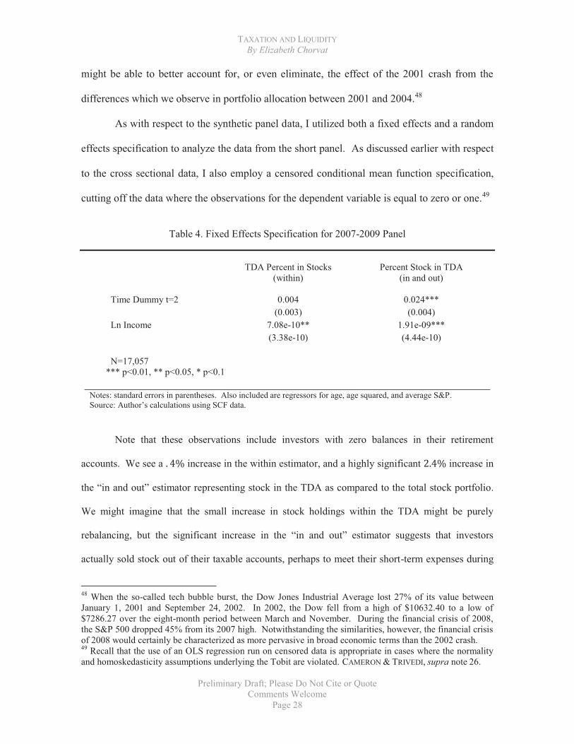
As with respect to the synthetic panel data, I utilized both a fixed effects and a random
effects specification to analyze the data from the short panel. As discussed earlier with respect
to the cross sectional data, I also employ a censored conditional mean function specification,
cutting off the data where the observations for the dependent variable is equal to zero or one.49
Table 4. Fixed Effects Specification for 2007-2009 Panel
TDA Percent in Stocks
(within)
Percent Stock in TDA
(in and out)
Time Dummy t=2 0.004 (0.003)
0.024*** (0.004)
Ln Income 7.08e-10** (3.38e-10)
1.91e-09*** (4.44e-10)
N=17,057
*** p<0.01, ** p<0.05, * p<0.1 ________________________________________________________________________
Notes: standard errors in parentheses. Also included are regressors for age, age squared, and average S&P. Source: Author’s calculations using SCF data.
Note that these observations include investors with zero balances in their retirement
accounts. We see a increase in the within estimator, and a highly significant increase in
the “in and out” estimator representing stock in the TDA as compared to the total stock portfolio.
We might imagine that the small increase in stock holdings within the TDA might be purely
rebalancing, but the significant increase in the “in and out” estimator suggests that investors
actually sold stock out of their taxable accounts, perhaps to meet their short-term expenses during
48 When the so-called tech bubble burst, the Dow Jones Industrial Average lost 27% of its value between January 1, 2001 and September 24, 2002. In 2002, the Dow fell from a high of $10632.40 to a low of $7286.27 over the eight-month period between March and November. During the financial crisis of 2008, the S&P 500 dropped 45% from its 2007 high. Notwithstanding the similarities, however, the financial crisis of 2008 would certainly be characterized as more pervasive in broad economic terms than the 2002 crash. 49 Recall that the use of an OLS regression run on censored data is appropriate in cases where the normality and homoskedasticity assumptions underlying the Tobit are violated. CAMERON & TRIVEDI, supra note 26.

TAXATION AND LIQUIDITY By Elizabeth Chorvat
Preliminary Draft; Please Do Not Cite or Quote
Comments Welcome Page 29
the downturn. In the next specification, the data for observations with either a zero or one as the
value of the dependent variable are censored before running the fixed effects specification again – a
so-called censored conditional mean function.
Table 5. Censored Conditional Mean Specification for 2007-2009 Panel
______________________________________________________________________________
TDA Percent in Stocks
(within)
Percent Stock in TDA (in and out)
Time Dummy t=2 0.0146 (0.010)
0.096*** (.012)
Ln Income 1.24e-09* (7.50e-10)
1.64e-09* (8.97e-10)
N=17,057
*** p<0.01, ** p<0.05, * p<0.1
_______________________________________________________________________ Notes: standard errors in parentheses. Also included are regressors for age, age squared, and average S&P. Source: Author’s calculations using SCF data.
We can see a increase in the within estimator, and a highly significant
increase in the “in and out” estimator. In the next specification, the data is analyzed using random
effects assumptions within a Tobit model on the panel data. Please refer to section C., below, for
the theoretical underpinnings of the application of the Tobit model for this data which relate to the
particular nature of the data as left censored.
See next page --

TAXATION AND LIQUIDITY By Elizabeth Chorvat
Preliminary Draft; Please Do Not Cite or Quote
Comments Welcome Page 30
Table 6. RE Tobit Specification for 2007-2009 Panel
____________________________________________________________________________________________________________
TDA Percent in Stocks (within)
Percent Stock in TDA
(in and out)
Time Dummy t=2 0.014** (0.007)
0.059*** (0.009)
Ln Income 2.18e-09*** (8.21e-10)
-4.63e-10*** (1.35e-09)
N=17,057
*** p<0.01, ** p<0.05, * p<0.1
________________________________________________________________________ Notes: standard errors in parentheses. Also included are regressors for age, age squared, and average S&P. Source: Author’s calculations using SCF data.
For the random effects specification, we see likewise very significant increases in stock
proportions held both within the retirement accounts, and in the proportion held inside the
retirement accounts as compared to total stock holdings by the investors. These are extremely
helpful and important findings. Of particular interest, the analysis of the 2007-2009 panel reveal
changes to portfolio allocation which were significant, and in the opposite direction of findings as a
result of the tax increase, lending confidence to the suggestion that the results observed between
2001 and 2004 were the result of the enactment of the dividend preference, and not as a
consequence of the 2002 market downturn, or changes in the composition of individuals entering or
leaving the survey.
We might, at this point, consider the results obtained from our alternate specifications.
First, consider the results from our analysis of the 2007-2009 “short panel” for the “within” and the
“in and out” estimators. Note especially the positive sign on the stock proportions, which are in the
opposite direction of our results for the effect of the tax change, suggesting that our results were
not influenced by the market crisis that occurred during the time period.

TAXATION AND LIQUIDITY By Elizabeth Chorvat
Preliminary Draft; Please Do Not Cite or Quote
Comments Welcome Page 31
Next, we turn to the results for the proportion of total stock in the retirement account.
Note that, for both estimators, the within and this so-called “in and out” estimator, all three
show positive effects such that, if we believe that the downturns are similar, we are more
confident in our general results.
C. Censored Data
One potential objection to the application of OLS to portfolio data is that our
observations are necessarily right censored, since we are dealing with proportions.50
Moreover, there is of necessity a lower bound of zero for these proportions, because
individuals are precluded under the applicable regulations from holding naked short positions
within a tax-deferred account.51 This means that the taxpayer’s net investment in all stocks
within the TDA cannot be below zero, when short and long positions are considered together.
Because the data are thus inherently double censored, the natural specification which lends
itself to modeling data with these restrictions would be a Tobit analysis of the effect of the
change in the tax law on portfolio allocation, with respect to both the within and within versus
without estimators.
Of course, the Tobit specifications are essentially the same as those detailed above with
some small differences. The latent variable in these specifications would be the optimal
proportion of stock in these accounts for the investor, assuming there were no limitations on
investment in the tax-deferred account. For the first specification we then have:
50 In theory, the proportions that we observe might be greater than one for the proportion of the retirement account that is held in stock, if the taxpayer borrowed to purchase stock in the account. There are rules precluding such transactions, however, so we return to our intuitive notion that the proportions observed should not exceed one. 51 Taxpayers may nonetheless engage in “covered” short position with respect to the same stock within a tax-deferred account, on the theory that that there is a net zero position within the tax-deferred account.

TAXATION AND LIQUIDITY By Elizabeth Chorvat
Preliminary Draft; Please Do Not Cite or Quote
Comments Welcome Page 32
Specification (1ˈ)
if
Likewise, we apply the same transformation to specification (2) given above, at page 13,
denoting each with a prime (ˈ) to indicate the Tobit transformation.
Table 7a. Tobit Specifications
____________________________________________________________________________________________________________
TDA Percent in
Stocks (1’)
Percent Stock in TDA (2’)
Dividend Tax -0.278***
(0.006) -0.115***
(0.008) Ln Income 0.134***
(0.002) 0.017***
(0.002) S & P July 1 1.38e-04***
(1.85e-05) -0.001***
(2.25e-05) N=24,166
*** p<0.01, ** p<0.05, * p<0.1 __________________________________________________________________________ Notes: standard errors in parentheses. Also included are regressors for age, age squared, and average S&P. Source: Author’s calculations using SCF data.
We can see that, while the coefficients are somewhat different than those observed
with the standard OLS specification, and larger, we observe the same basic story employing
the Tobit models as with the use of the OLS. Note that, because Tobit is regarded as fragile to
violations of the normality and homoskedasticity assumptions, it is necessary to test the

TAXATION AND LIQUIDITY By Elizabeth Chorvat
Preliminary Draft; Please Do Not Cite or Quote
Comments Welcome Page 33
validity of these assumptions. 52 When a LaGrange multiplier test is run on the error terms, the
p-value returned is indistinguishable from zero. Therefore, we can reject the hypothesis that
the error terms are homoskedastic and normally distributed,
One way to address the problem of the fragility of the Tobit assumptions is to employ
an OLS regression run on the observations where there are positive balances in the tax deferred
accounts. This is appropriate in cases where the normality and homoskedasticity assumptions
underlying the Tobit are violated.53 This is sometimes referred to as a censored conditional
expectation.
Table 7b. Censored Conditional Expectation
____________________________________________________________________________________________________________
TDA Percent in Stocks
(1)
Percent Stock in TDA (2)
Dividend Tax -0.0548***
(0.0047) -.1183*** (0.0030)
Ln Income 0.0472*** (0.0012)
0.0835*** (0.002)
S & P July 1 2.45e-5* (1.0e-5)
-0.001*** (0.000)
N=17,684
*** p<0.01, ** p<0.05, * p<0.1 __________________________________________________________________________
Notes: standard errors in parentheses. Also included are regressors for age, age squared, and average S&P. Source: Author’s calculations using SCF data.
52 The test for sensitivity of the Tobit model to nonnormality and heteroskedasticity is conducted by computing the LaGrange multiplier statistic for testing the Tobit specification against the alternative of a model that is nonlinear in the regressors and contains an error term that can be heteroskedastic and nonnormally distributed. The test is carried out by taking a Box-Cox transformation of the dependent
variable and testing whether the parameter is equal to one. A rejection of the null would indicate that the Tobit specification is unsuitable, because an alternative value for lambda would be necessary to return the linearity, homoskedasticity, and normality assumptions that are necessary for consistent estimation. See D. Vincent, Btobit: Stata Module to Produce a Test of the Tobit Secification, at http://ideas.repec.org/c/boc/bocode/s457163.html (2010). 53 A. COLIN CAMERON & PRAVIN K. TRIVEDI, MICROECONOMETRICS USING STATA 578-541 (2009).
TAXATION AND LIQUIDITY By Elizabeth Chorvat
Preliminary Draft; Please Do Not Cite or Quote
Comments Welcome Page 34
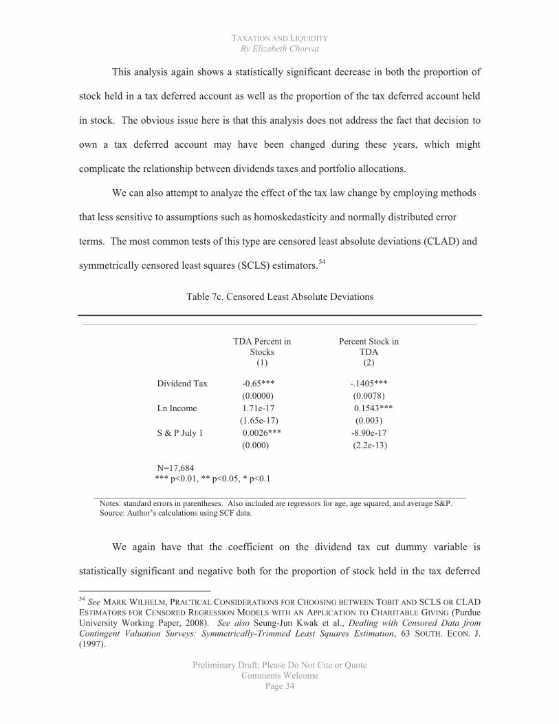
This analysis again shows a statistically significant decrease in both the proportion of
stock held in a tax deferred account as well as the proportion of the tax deferred account held
in stock. The obvious issue here is that this analysis does not address the fact that decision to
own a tax deferred account may have been changed during these years, which might
complicate the relationship between dividends taxes and portfolio allocations.
We can also attempt to analyze the effect of the tax law change by employing methods
that less sensitive to assumptions such as homoskedasticity and normally distributed error
terms. The most common tests of this type are censored least absolute deviations (CLAD) and
symmetrically censored least squares (SCLS) estimators.54
Table 7c. Censored Least Absolute Deviations
____________________________________________________________________________________________________________
TDA Percent in Stocks
(1)
Percent Stock in TDA (2)
Dividend Tax -0.65***
(0.0000) -.1405*** (0.0078)
Ln Income 1.71e-17 (1.65e-17)
0.1543*** (0.003)
S & P July 1 0.0026*** (0.000)
-8.90e-17 (2.2e-13)
N=17,684
*** p<0.01, ** p<0.05, * p<0.1 __________________________________________________________________________
Notes: standard errors in parentheses. Also included are regressors for age, age squared, and average S&P. Source: Author’s calculations using SCF data.
We again have that the coefficient on the dividend tax cut dummy variable is
statistically significant and negative both for the proportion of stock held in the tax deferred
54 See MARK WILHELM, PRACTICAL CONSIDERATIONS FOR CHOOSING BETWEEN TOBIT AND SCLS OR CLAD ESTIMATORS FOR CENSORED REGRESSION MODELS WITH AN APPLICATION TO CHARITABLE GIVING (Purdue University Working Paper, 2008). See also Seung-Jun Kwak et al., Dealing with Censored Data from Contingent Valuation Surveys: Symmetrically-Trimmed Least Squares Estimation, 63 SOUTH. ECON. J. (1997).

TAXATION AND LIQUIDITY By Elizabeth Chorvat
Preliminary Draft; Please Do Not Cite or Quote
Comments Welcome Page 35
account as opposed to outside of it and the proportion of the tax deferred account held as stock.
One point that is surprising is the magnitude of the coefficient for the specification analyzing
the effect of the proportion of the TDA held in stocks. This appears to indicate that there was a
sixty five percentage point drop in the proportion of the tax deferred accounts held as stock.
This seems quite large.
This large change in the within variable likely has to do with the particular method
used to analyze the change. Unlike least squares analysis, which is sensitive to changes in the
expected value of the dependent variable, absolute deviations methods are sensitive to changes
in the median of the dependent variable. If the values of the dependent variable are grouped, it
is possible that a small change in the overall distribution might change the median more than it
does the average.55
We can see that this is the case here. Among those who had positive balances in their
tax deferred account, the median value of the proportion of the account held in stock before the
tax change was 100% percent. The median value after for those who had positive balances
was 35%. However there was only a 14% change in the average value. We can see that while
absolute deviations methods are not as sensitive to errors, we must remember they are telling
us about the change to median values rather than changes to average values.
Another method of analyzing censored data which is not as sensitive to assumptions
about the error terms is symmetrically trimmed least squares.
See next page --
55 To see this, imagine that there is a group of 100 observations, 49 of which have a value of zero and 51 of which have a value of 1. The median value is then 1. The mean is .51 If two observations switch from one to zero, the median switches from one to zero, while the mean only drops to .49.

TAXATION AND LIQUIDITY By Elizabeth Chorvat
Preliminary Draft; Please Do Not Cite or Quote
Comments Welcome Page 36
Table 8d. Symmetrically Trimmed Least Squares
____________________________________________________________________________________________________________
TDA Percent in
Stocks (1)
Percent Stock in TDA (2)
Dividend Tax -0.842**
(0.328) -.1234*** (0.0159)
Ln Income 0.132*** (0.0298)
0.1026*** (0.004)
S & P July 1 0.0001 (0.0007)
-0.0018*** (0.0002)
N=17,057
*** p<0.01, ** p<0.05, * p<0.1 __________________________________________________________________________ Notes: standard errors in parentheses. Also included are regressors for age, age squared, and average S&P. Source: Author’s calculations using SCF data.
We see again that the signs of the coefficients on the dummy variables for the tax changes
are negative and statistically significant. We have the same issue here as we did above with the
proportion of the TDA held in stock. That is, the analysis indicates that there was a very large
change in the proportion of the tax deferred accounts held in stock We can see that the
confidence interval for this coefficient runs from about a 19% to a 148% drop in the proportion
of the IRA held in stock. This is an enormous range. Therefore, this would not be a good
method for attempting to estimate what the actual change was. However, even with this very
low degree of precision, we see that the analysis tells us that the effect was negative and
statistically significant.
Considering the opposite sign and the significance of the changes in stock holdings
during the market downturn which occurred during the period, we are all that much more
confident in our findings. Investor behavior in response to the 2003 dividend preference

TAXATION AND LIQUIDITY By Elizabeth Chorvat
Preliminary Draft; Please Do Not Cite or Quote
Comments Welcome Page 37
appears to be consistent with the behavior which would be predicted by the tax-efficient model
of behavior described in Tobin (1958).
IV. THE DISTRIBUTION OF PORTFOLIO RESPONSE
The behavioral effect of tax rate changes, more technically framed as the elasticity of
response, has been of interest to economists since the early twentieth century.56 We may want
to examine how the reductions in the proportion of stock inside and outside of the retirement
accounts were distributed among income groups. This may help us understand the dynamics
of the effect on the tax change on portfolio choice.
The basic theory discussed at the beginning of the paper does not tell us very much
about how we would expect the portfolio allocations to be distributed across income groups.
The only unambiguous prediction which theory provides is that we expect for the proportions
of stock in the TDA to decrease; it does not tell us how much we would expect it to decrease,
nor does it tell us precisely what factors we would expect to influence this decision other than
the tax rates. While we might expect that those in the lowest income groups would value a
marginal increase in liquidity more highly than those in the upper income groups,57 it may also
be that the lower-income households had less in their TDAs to begin with, so that there is less
ability to create liquidity from their portfolios. The theory only predicts that for each group we
would expect both the proportion of stock within and without the TDAs should decrease.
Therefore, the analysis here does not technically test the main hypothesis, but rather merely
allows us a richer understanding of the effects of the tax.
56 The basic notion of taxing elastic and inelastic behavior dates back to Frank P. Ramsey, A Contribution to the Theory of Taxation, 37 Economic Journal 47 (1927). See also James A. Mirrlees, An Exploration in the Theory of Optimum Income Taxation, 38 Rev. Econ. Stud. 175 (1971) (extending the notion of Ramsey taxation to the taxation of income from labor). 57 This follows because if one has more assets it likely easier to keep a portion of them liquid. In addition, since we are sorting by income, those at the highest income groups have a ready source of liquidity, namely the cash flow of their income.
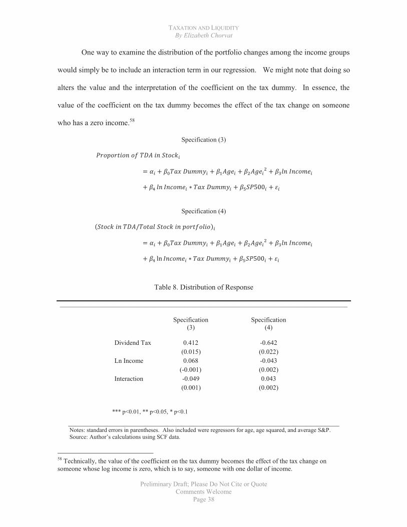
TAXATION AND LIQUIDITY By Elizabeth Chorvat
Preliminary Draft; Please Do Not Cite or Quote
Comments Welcome Page 38
One way to examine the distribution of the portfolio changes among the income groups
would simply be to include an interaction term in our regression. We might note that doing so
alters the value and the interpretation of the coefficient on the tax dummy. In essence, the
value of the coefficient on the tax dummy becomes the effect of the tax change on someone
who has a zero income.58
Specification (3)
Specification (4)
Table 8. Distribution of Response
____________________________________________________________________________________________________________
Specification
(3) Specification
(4)
Dividend Tax 0.412 (0.015)
-0.642 (0.022)
Ln Income 0.068 (-0.001)
-0.043 (0.002)
Interaction -0.049 (0.001)
0.043 (0.002)
*** p<0.01, ** p<0.05, * p<0.1 __________________________________________________________________________ Notes: standard errors in parentheses. Also included were regressors for age, age squared, and average S&P. Source: Author’s calculations using SCF data.
58 Technically, the value of the coefficient on the tax dummy becomes the effect of the tax change on someone whose log income is zero, which is to say, someone with one dollar of income.

TAXATION AND LIQUIDITY By Elizabeth Chorvat
Preliminary Draft; Please Do Not Cite or Quote
Comments Welcome Page 39
The equations estimated above seem to tell us that the correlation between the dividend
tax reduction and the proportion of the retirement account invested in stock is highly
dependent on the income of the family. For poorer families, the tax changes seem correlated
with an increase in the proportion of the retirement accounts held in stock, while for those with
median income (actually, even below median income) and above, the effect of the tax changes
are correlated with a decrease in the proportion of the retirement account held in stock. By
contrast, it would appear that, based on the linear equation derived from the analysis above, we
would predict that lower income households decreased the proportion of their stock held in
their retirement accounts while, for higher income households, they decreased it by a much
lower amount. That is, to evaluate the predicted value for any given household, we have to
include income twice. So, for example, at the median income in the survey, we have that the
coefficient on tax variable for the proportion of the retirement account held in stock has the
value -0.122, implying that the tax change reduced the proportion by about 12 percentage
points.59 The equivalent result for the portion of total stock that is allocated to the TDA is -
0.305, implying a reduction of about 31 percentage points for those with median income.
However, the specifications given above impose the restriction that the effects take the
same form for all income groups. To allow for nonlinear effects, we might separate the
population into different groups and then examine the average effect of the tax changes for
each of these different income groups separately. This might tells us more than the coefficient
on an interaction term by allowing for the relationship to be different in a nonlinear fashion.
First, we examine the proportion of the TDA invested in stock. I use the same three
groups that I used above for the summary statistics. We see that the effect for those making
more than $200,000 is a larger drop than was true for the general population (of about 29%).
59 Mean log income is 11.14636 and median log income is 10.93311.

TAXATION AND LIQUIDITY By Elizabeth Chorvat
Preliminary Draft; Please Do Not Cite or Quote
Comments Welcome Page 40
Table 9. Distribution of Response: Proportion of TDA in Stock
< $100,000
$100,000-$200,000 > $200,000
Dividend Tax -0.058 (.002)
-0.253 (.008)
-0.290 (.005)
*** p<0.01, ** p<0.05, * p<0.1
______________________________________________________________________________________ Notes: standard errors in parentheses. Also included are regressors for age, age squared, and average S&P. Source: Author’s calculations using SCF data.
We see that for those between 100,000 and 200,000 we still have a large negative
effect of about 25%. Finally for those who had family incomes of less than $100,000, we saw
a much smaller drop. We can note that for all of these groups the effect of the tax change was
still to reduce the amount of the TDAs allocated to stock.
To sum up, we see that the reduction in the tax rate on dividends is correlated with a
reduction in the proportion of the TDAs allocated to stock for each of the three groups. The
largest reduction was found among those with the highest income. Those in the next group had
a similar, although slightly smaller, reduction. We can see that the reductions were much
stronger among those earning more than $100,000 than those families with incomes below this.
In short, we see that the effect of the tax change is very dependent upon the income of the
family.
We can conduct a similar analysis on the other variable, the proportion of stock held in
retirement accounts versus the stock held outside of the retirement account. Under this
analysis, we have:
See next page –

TAXATION AND LIQUIDITY By Elizabeth Chorvat
Preliminary Draft; Please Do Not Cite or Quote
Comments Welcome Page 41
Table 10. Distribution of Response: Proportion of Stock Held in TDA
< $100,000
$100,000-$200,000 > $200,000
Dividend Tax -0.208 (.005)
-0.054 (.008)
-0.051 (.005)
*** p<0.01, ** p<0.05, * p<0.1
______________________________________________________________________________________ Notes: standard errors in parentheses. Also included are regressors for age, age squared, and average S&P. Source: Author’s calculations using SCF data.
For households with incomes over $100,000 we see a drop of a little over five
percentage points. But, for those households with incomes less than $100,000, we saw a much
larger drop. This is almost the exact reverse of what we saw with the proportion of the
retirement accounts held in stock.
Above we saw that the drop in the proportion of the IRA which is allocated to stock is
something that occurs mostly among higher (or at least higher than median income) families.
This is in contrast to what happens for the proportion of stock held in the TDA versus total
stock held by the family, where that proportion goes down with income, although not
monotonically.
We can bring into this analysis some of the summary statistics discussed above at
Section II, Table I. We see that the proportion TDA stock holdings to total stock holdings
dropped substantially for the lowest of three income groups. We can see that this group
essentially doubled its stock holdings outside of the TDA, while they did not double the size of
their TDAs (and also slightly reducing the proportion of the TDA allocated to stocks). This
resulted in a high proportion of their stock holdings being held outside of their TDAs.
Thus, for the lowest income households, the largest effect of the reduction in taxes on
dividends seems to have been an increase of their holdings of stock outside of the TDA. Given
that this was one of the goals of the tax law changes, it is interesting to note that this group
TAXATION AND LIQUIDITY By Elizabeth Chorvat
Preliminary Draft; Please Do Not Cite or Quote
Comments Welcome Page 42
substantially increased its holdings of stocks outside of TDAs. There are a variety of reasons
why this might have occurred. For these households, liquidity may matter more, and the
limitations imposed by the TDAs are too restrictive to result in an attractive investment. By
reducing the income tax on income tax on investments for this group this increased the amount
of stock investment substantially. Of course, without further analysis this is essentially a just-
so-story.
For the highest income group we also observe that there was an increase of over
$400,000 in the amount of stock held outside of TDAs. So we see that for these two groups,
the tax changes seem to have increased their stock holding outside of TDAs.
One odd point is that outside stockholdings by those in the middle income group seem
to have dropped. Interestingly, so did the size of the TDAs held by this group, as well the
proportion of their TDAs allocated to stocks. This seems to indicate that this group reduced its
stock holding and retirement savings during this period.
We might be concerned that perhaps some easily controlled for factors such as the
value of the stock market at given time might be the true factor that is responsible for the
changes discussed in this section, rather than the tax change. The summary statistics discussed
in Section II, supra, do not have the ability to control for these types of effects. One way to
examine whether this is a real possibility would be to run separate regressions for different
income groups to see if the value of the coefficient on the dummy variable for the tax change is
different for the different groups. In this case, the dependent variable is the amount of stock
outside of the TDA, and then we use as control variables such factors as the tax change and the
value of the S&P 500 around the time of the survey and other factors such as age and age
squared.
Doing this for the different groups gives us the following results:
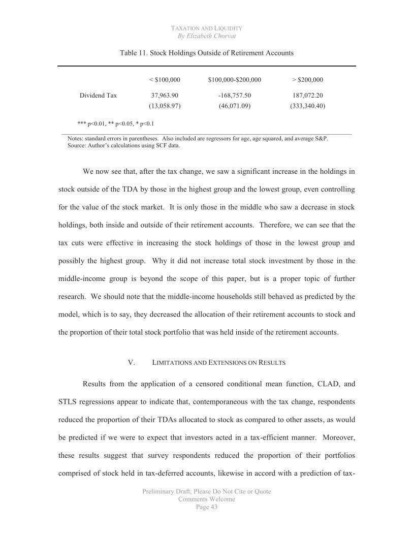
TAXATION AND LIQUIDITY By Elizabeth Chorvat
Preliminary Draft; Please Do Not Cite or Quote
Comments Welcome Page 43
Table 11. Stock Holdings Outside of Retirement Accounts
< $100,000
$100,000-$200,000 > $200,000
Dividend Tax 37,963.90 (13,058.97)
-168,757.50 (46,071.09)
187,072.20 (333,340.40)
*** p<0.01, ** p<0.05, * p<0.1
______________________________________________________________________________________ Notes: standard errors in parentheses. Also included are regressors for age, age squared, and average S&P. Source: Author’s calculations using SCF data.
We now see that, after the tax change, we saw a significant increase in the holdings in
stock outside of the TDA by those in the highest group and the lowest group, even controlling
for the value of the stock market. It is only those in the middle who saw a decrease in stock
holdings, both inside and outside of their retirement accounts. Therefore, we can see that the
tax cuts were effective in increasing the stock holdings of those in the lowest group and
possibly the highest group. Why it did not increase total stock investment by those in the
middle-income group is beyond the scope of this paper, but is a proper topic of further
research. We should note that the middle-income households still behaved as predicted by the
model, which is to say, they decreased the allocation of their retirement accounts to stock and
the proportion of their total stock portfolio that was held inside of the retirement accounts.
V. LIMITATIONS AND EXTENSIONS ON RESULTS
Results from the application of a censored conditional mean function, CLAD, and
STLS regressions appear to indicate that, contemporaneous with the tax change, respondents
reduced the proportion of their TDAs allocated to stock as compared to other assets, as would
be predicted if we were to expect that investors acted in a tax-efficient manner. Moreover,
these results suggest that survey respondents reduced the proportion of their portfolios
comprised of stock held in tax-deferred accounts, likewise in accord with a prediction of tax-
TAXATION AND LIQUIDITY By Elizabeth Chorvat
Preliminary Draft; Please Do Not Cite or Quote
Comments Welcome Page 44
efficient behavior.60 There are, however, some ancillary issues that arise from the limitations
on the available data that are discussed in this Part.
A. The “Respondents’ Estimation” Variable
In the course of calculating the stock proportion variable for the 2004 SCF data, I
attempted to use the new-to-2004 “respondents’ estimation” variable, in order to determine
how well it compares with the Bergstresser and Poterba variable, as we might imagine that this
variable could afford a more direct method of calculating the percentage of tax-deferred
accounts which are constituted of stock.61 With the “short panel” data, we should be all the
more well-equipped to gauge the reliability of the Bergstresser and Poterba estimator of
portfolio allocation within the deferral accounts although, as discussed earlier, the
Bergstresser and Poterba estimator appears to perform well as a proxy for the more direct
measure of portfolio allocation within TDAs introduced with the 2004 Survey.
B. Assumptions Inherent in the Model
Important limitations upon any model are the assumptions that presuppose constancy
throughout the periods observed. One important factor which might not have remained
constant between 1998 and 2007 is the dividend policy of corporations. If the dividend policy
of corporations significantly changes, then it is not so clear that the tax efficiency of holding
corporate stock would have been impacted by the 2003 legislation. To illustrate, consider a
60 See, e.g., Brad M. Barber & Terrance Odean, Are Individual Investors Tax Savvy?, 88 J. PUB. ECON. 419 (2004) (utilizing individual-level data to examine trading behavior). 61 In order to further test the causality which we might infer from these results, one might attempt to obtain data from mutual fund companies or other investment advisors on the actual changes made by individuals to both their taxable and tax-deferred accounts. In this analysis, I actually utilize the dollar amount of stock invested within tax-deferred retirement vehicles in 2001 divided by the total dollar amount invested in retirement vehicles for that year versus the dollar amount of stock invested within tax-deferred retirement vehicles in 2004 divided by the total dollar amount invested in retirement vehicles for that year, because of issues relating to changes in the value of the market, in order that the comparison reflects more than mere changes in market value.

TAXATION AND LIQUIDITY By Elizabeth Chorvat
Preliminary Draft; Please Do Not Cite or Quote
Comments Welcome Page 45
corporation which, prior to the change in the tax rules, did not pay dividends. This stock
would not have been most prudently held within a deferral account, unless one was expecting
to actively trade such shares, because any accession to the value of the stock would have been
provided deferral under the Code until a realization event, such as the sale or transfer of the
shares. If after this change in the rules, such a corporation began to pay dividends, then the
character of the asset has changed from an asset which clearly should not be held inside of a
deferral account to one which might well benefit from being held in a TDA, depending upon
the relevant tax and non-tax considerations.
C. Constancy of Liquidity Value
For purposes of the model described at Part I, we assume constancy of liquidity value.
Given the heterogeneity of response we observe among different income classes of households,
this may indeed be a strong assumption. Of course, any change in the value ascribed to
liquidity will necessarily alter the allocation of any particular asset, as between tax-deferred
and fully taxable accounts. Many models would predict that, as the economic situation of the
taxpayer changes, the demand for liquidity will also change. It is possible that changes in
liquidity value may explain some of the changes in portfolio allocation which we observe. The
natural prediction, however, would be that the demand for liquidity should go up in bad
economic times and down in relatively good economic times. Our empirical findings appear to
run counter to this intution. That is, as the economy improved, at least as measured by the
S&P 500, the demand for liquidity (which is to say, stock outside of the tax-deferred account)
appeared to increase. Even so, we must always be mindful of the assumption that the
respondents’ taste for liquidity is assumed to be constant in our simple model, even though
many models would argue otherwise.

TAXATION AND LIQUIDITY By Elizabeth Chorvat
Preliminary Draft; Please Do Not Cite or Quote
Comments Welcome Page 46
Conclusions
The conclusions we might draw from a principled review of the empirical results in
this study are both positive and normative. First, from a positive standpoint, it appears that
empirical results based on regression analyses of Survey of Consumer Finances data suggest that
investors reallocated their stock portfolios in a tax efficient manner, moving stocks from tax
preferred retirement accounts to taxable accounts. Of particular interest, while the behavioral
response to the decrease in the tax rate – effectively, the decrease in the price of holding stock
in liquid form – was strong among the wealthy, it was stronger still among the relatively poorer
households, with an increase in total stock holdings almost twenty times as large as among the
highest income households.62 Curiously, while the middle-income households responded to
the lower cost of liquidity in a tax-efficient manner, theirs was a distinctly smaller response.
Therefore, we can see that the tax cuts were effective in increasing the stock holdings of those
in the lowest income households, and possibly the highest-income households. Why the tax
cut did not increase total stock investment by those in middle-income households is beyond the
scope of this paper, but is a proper topic of further research. We should note that the middle-
income households still behaved as predicted by the model, which is to say, they decreased the
allocation of their retirement accounts to stock and the proportion of their total stock portfolio
that held inside of the retirement accounts.
The normative conclusions suggested by these results may be distinguished as
microeconomic effects and macroeconomic effects. At the microeconomic level, we know
62 Returning to the summary statistics and, in particular, the average stock holdings outside of the retirement accounts, note the difference in the behavioral response of the lowest and highest income households. The lower-income households increased their liquid stock holdings by 113%, while the upper-income households increased their liquid holdings by approximately 7%.
TAXATION AND LIQUIDITY By Elizabeth Chorvat
Preliminary Draft; Please Do Not Cite or Quote
Comments Welcome Page 47
that, because asset location affects portfolio performance, a tax-efficient response to legislative
reform generates positive and significant effects for welfare in retirement.63
A more subtle microeconomic prediction would be that a reallocation of stock away
from tax-preferred retirement accounts into taxable accounts would tie consumption to market
changes. Because a larger proportion of stock would be reallocated in favor of in liquid
accounts, these investments are made available for consumption, and are subject to the
traditional wealth effects associated with market changes. This is consistent with the results in
the panel study, where the 2008 market downturn was associated with the sale of stock in
liquid accounts, increasing the proportion of stock portfolios held in retirement accounts.
At the macroeconomic level, a reallocation of stock into liquid accounts would
increase the taxable base. This increase, however, would be offset by a larger decrease in the
taxable base as bonds – which are fully taxable at ordinary rates – are reallocated to tax
preferred accounts.64 This net decrease in the taxable base would be disfavored from a policy
perspective. Moreover, the shift from equity investments to debt instruments for retirement
savings would have uncertain implications for the future growth in those accounts, and the
resulting household security for retirement.
63 Shoven & Sialm, supra note 11, at 36-37. The gains to tax-efficient portfolio allocation are enhanced if the stocks and bonds differ substantially in the extent to which their returns are distributed to the asset holder. Id. at 36. 64 John B. Shoven & Clemens Sialm, Asset Allocation in Tax-Deferred and Conventional Savings Accounts, 88 J. PUB. ECON. 23, 24 (2003). By “bonds” I mean of course corporate and U.S. federal government bonds, the interest on which is fully taxable at ordinary rates, and not state or municipal bonds. IRC §§ 61, 103. Investors are taxed at ordinary rates as well on interest received on original issue discount or OID debt, as well as the effective interest rate implied in the bond. IRC §§ 1271-1274. Government bonds, which constitute a significant share of individual portfolios, are fully taxable at ordinary rates at the federal (although not the state) level. Individuals would likely reallocate both corporate and U.S. federal government debt.

TAXATION AND LIQUIDITY By Elizabeth Chorvat
Preliminary Draft; Please Do Not Cite or Quote
Comments Welcome Page 48
Appendix A The SCF questions related to the total amount invested in tax-deferred accounts:
X3610 How much in total is in your [IRA(s)/Keogh account(s)/IRA and Keogh accounts]? X3620 How much in total is in your spouse's [IRA(s)/Keogh account(s)/IRA and Keogh
accounts]? X3630 How much in total is in your partner's [IRA(s)/Keogh account(s)/IRA and Keogh
accounts]?
SCF questions relating to the allocation of the funds in the tax-deferred account: X3631 How is the money in (this/all of these) IRA and Keogh accounts(s) invested? Is
most of it in CDs or other bank accounts, most of it in stocks, most of it in bonds or similar assets, or what?
How is the money in (all) your family's IRA and Keogh account(s) invested? Is
most of it in CDs or other bank accounts, most of it in stocks, most of it in bonds or similar assets, or what?
1. *CDs/Bank accounts; "money market" 2. Bonds/Similar assets; T-Bills; treasury notes 4. Combinations of 1, 2, & 3 ; "mixed"/"diversified" -- NFS 5. Combination of 2 & 3 above 6. Combination of 1 & 2 above 11. Universal life policy or other similar insurance product 12. Annuity 13. Commodities 14. Real estate/mortgages 15. Limited partnership/other similar investment 16. Brokerage account/cash management account (CMA) -7. *Split/Other 0. Inap. (No IRA/Keogh accounts: X3601^=1)
For the 2004 and 2007 the following question was added with regard to tax-deferred accounts:
X6556 About what percent is in stocks(in your [IRA(s)/Keogh account(s)/IRA and Keogh accounts])
X6564 About what percent is in stocks(in your spouse’s [IRA(s)/Keogh account(s)/IRA and Keogh accounts])
X6572 About what percent is in stocks(in your partner’s [IRA(s)/Keogh account(s)/IRA and Keogh accounts])
Code percent * 100
It is based on the answer to this question that the more precise estimates of the
percentage of the tax-deferred accounts invested in stock was determined.

TAXATION AND LIQUIDITY By Elizabeth Chorvat
Preliminary Draft; Please Do Not Cite or Quote
Comments Welcome Page 49
Appendix B
Comparative Statics of Portfolio Allocation
To analyze the comparative statics of the allocation of stock between fully taxable and
tax deferred accounts, which is to say, that a, the proportion of stock allocated to taxable
accounts, must increase as decreases, we can utilize the implicit function theorem, which
gives us that:
Recall, from equation (2), we have that the investor optimizes utility over his portfolio,
taking into account the tax rate, rate of return, and liquidity value in the following manner,
where the proportion of the portfolio outside of the deferral account is:
This gives us that:
We can see that, if the numerator and denominator are both negative, then the
derivative will be negative. In other words, if the tax rate increases, the proportion of
stock held outside of the TDA, in taxable accounts, will decrease. Equivalently a, the
proportion of stock allocated to taxable accounts, will increase as decreases.
Let us examine the right-hand side, then, to see when will be negative. We can
see that the denominator of the right-hand side will be negative if, as assumed, is
concave. If we examine the numerator, we see that the first term, , is
� �� � � �� � � �1 1 1 1 1 0S r L aS r S r� �� ��� � � � �

TAXATION AND LIQUIDITY By Elizabeth Chorvat
Preliminary Draft; Please Do Not Cite or Quote
Comments Welcome Page 50
negative, because is positive. The second term,
, is positive, because of the term and the assumption of concavity for .
Given, then, that the first term is negative and the second is positive, we must determine the
conditions under which the sum of these two terms in the numerator will result in a negative
value.
If the sum of these terms is negative, then we have that:
We can rewrite this as:
If we divide both sides of the inequality by , we will switch the sign of the
inequality, because we are dividing by a negative number. This gives us:
We can then move to the other side of the
inequality (subtracting it from both sides), which give us:
Next, we can divide both sides of the inequality by . We note
that, owing to the concavity of , this term is negative, so we then have:
Or, equivalently, multiplying both sides by -1, we could write:
Recalling once again that the liquidity function is concave, this inequality
condition tells us that the rate of decline in the marginal value of liquidity needs to be very
TAXATION AND LIQUIDITY By Elizabeth Chorvat
Preliminary Draft; Please Do Not Cite or Quote
Comments Welcome Page 51
small relative to the marginal value of liquid wealth. This is saying that the value of liquidity
to investors does not decline so fast that, if the investor doubled the amount of liquid wealth,
there would be a one unit change in the marginal value of liquid wealth. Another way to
conceptualize this intuition would be to think of the investor’s liquidity function as “up-
weighting” the value of liquid wealth. Thus, the comparative statics tell us that, if the amount
of a liquid asset were to double, the marginal value of liquid wealth cannot fall by more than
1 unit of “up-weight.”
We see from equation that, at the optimum,
. This is to say that the marginal value of a liquid dollar will be equal to
the marginal value from gaining a tax advantage. We can see, that for any realistic set of
values 2 > for all wealth levels and, irrespective of the size of the increase in liquid
wealth, the marginal value of liquidity can never drop by 1 unit, so the requirement of equation
or, equivalently, of equation is very likely met. In other words, for to be
negative, equation or, equivalently, equation must be true. The intuition here is
that the rate of decline in the value of a liquid dollar has to be small in relation to the value of
the liquid dollar.
TAXATION AND LIQUIDITY By Elizabeth Chorvat
Preliminary Draft; Please Do Not Cite or Quote
Comments Welcome Page 52
Appendix C
Comparative Statics of the Allocation within Tax Deferred Accounts
For completeness, we can demonstrate that, if the amount of stock held in the tax
deferred account declines, the proportion of the tax deferred account held as stock will also
decline. To analyze the allocation of the tax deferred account as between stock and other
assets, we begin by assuming that the foregoing model regarding the allocation of stock
between the taxable and taxed deferred accounts is correct. Here, because we are merely
attempting to predict the sign of the change in the proportion of stock in the TDA following the
rate change, we can allow for an approximation of the actual ratio. We do not know the actual
ratio, because the rate change might affect non-stock as well as stock assets. If we assume that
the amount of non-stock assets in the tax deferred account are either constant or increasing65
then, we can see that, if the amount of the stock in the account decreases,66 then it must be the
case that the ratio:
will decline, where represents the stock held in the tax deferred account, and
represents the non-stock assets held in the tax deferred account. We can see this by noting that
the derivative of this ratio with respect to stock in the account, , will be:
by the quotient rule.
65 There would be no reason to decrease the non-stock assets in the account, because the method of taxation for non-stock assets has not changed. 66 See Appendix B.

TAXATION AND LIQUIDITY By Elizabeth Chorvat
Preliminary Draft; Please Do Not Cite or Quote
Comments Welcome Page 53
We can then see that, because this fraction must necessarily be positive under our
assumptions, therefore the derivative is positive. This of course implies that a decline in the
absolute amount of the stock in the tax deferred account will result in a decline in the
proportion of the tax deferred account held as stock. Therefore, we can expect that, if the
amount of stock held in the tax deferred account declines, the proportion of the tax deferred
account held as stock will also decline.