Tax Cuts for Whom - The National Bureau of Economic … Cuts For Whom? Heterogeneous Effects of Income Tax Changes on Growth and Employment Owen M. Zidar NBER Working Paper No. 21035

NBER WORKING PAPER SERIES

TAX CUTS FOR WHOM? HETEROGENEOUS EFFECTS OF INCOME TAX CHANGES ON GROWTH AND EMPLOYMENT

Owen M. Zidar

Working Paper 21035http://www.nber.org/papers/w21035

NATIONAL BUREAU OF ECONOMIC RESEARCH1050 Massachusetts Avenue

Cambridge, MA 02138March 2015

Revised February 2017

I am grateful to Alan Auerbach, Dominick Bartelme, Alex Bartik, Marianne Bertrand, David Card, Gabe Chodorow-Reich, Austan Goolsbee, Ben Keys, Pat Kline, Attila Lindner, Zachary Liscow, Neale Mahoney, Atif Mian, John Mondragon, Enrico Moretti, Matt Notowidigdo, Christina Romer, David Romer, Jesse Rothstein, Emmanuel Saez, Jim Sallee, Andrew Samwick, Amir Sufi, Laura Tyson, Johannes Wieland, Dan Wilson, Danny Yagan, and Eric Zwick for helpful comments and Dan Feenberg for generous help with TAXSIM. I am especially thankful to Amir Sufi as well as Marianne Bertrand and Adair Morse for generously sharing data with me. This project grew out of an undergraduate research project that I worked on with Daniel Cohen, and I am grateful to him and Jim Feyrer for input on the paper at its inception. Stephanie Kestelman, Stephen Lamb, Francesco Ruggieri, Karthik Srinivasan, and John Wieselthier provided excellent research assistance. This work is supported by the Kathryn and Grant Swick Faculty Research Fund at the University of Chicago Booth School of Business. The latest version of this paper can always be found at http://faculty.chicagobooth.edu/owen.zidar/. The views expressed herein are those of the author and do not necessarily reflect the views of the National Bureau of Economic Research.

NBER working papers are circulated for discussion and comment purposes. They have not been peer-reviewed or been subject to the review by the NBER Board of Directors that accompanies official NBER publications.

© 2015 by Owen M. Zidar. All rights reserved. Short sections of text, not to exceed two paragraphs, may be quoted without explicit permission provided that full credit, including © notice, is given to the source.

Tax Cuts For Whom? Heterogeneous Effects of Income Tax Changes on Growth and Employment Owen M. ZidarNBER Working Paper No. 21035March 2015, Revised February 2017JEL No. E32,E62,H2,H20,H31,N12

ABSTRACT

This paper investigates how tax changes for different income groups affect aggregate economic activity. I construct a measure of who received (or paid for) tax changes in the postwar period using tax return data from NBER's TAXSIM. I aggregate each tax change by income group and state. Variation in the income distribution across U.S. states and federal tax changes generate variation in regional tax shocks that I exploit to test for heterogeneous effects. I find that the positive relationship between tax cuts and employment growth is largely driven by tax cuts for lower-income groups, and that the effect of tax cuts for the top 10% on employment growth is small.

Owen M. ZidarUniversity of ChicagoBooth School of Business5807 South Woodlawn AvenueChicago, IL 60637and [email protected]

There are two ideas of government. There are those who believe that if you just legislate tomake the well-to-do prosperous, that their prosperity will leak through on those below. TheDemocratic idea has been that if you legislate to make the masses prosperous their prosperitywill find its way up and through every class that rests upon it.

—William Jennings Bryan (July, 1896)

The consequences of changing tax policy for different groups are fiercely debated. Some policy

makers maintain that tax changes for high-income earners “trickle down” and are the most

effective way to affect prosperity. They argue that higher marginal tax rates for top-income

taxpayers lead to large distortions in labor supply, investment, and hiring, so tax cuts for

top-income taxpayers most effectively increase aggregate economic activity. Others, however,

contend the opposite. They argue that lower-income groups have higher marginal propensities

to consume and disincentives to work from means-tested benefits, so tax cuts for lower-income

groups generate sizable consumption and labor supply responses, and thereby, more overall

activity. Do tax changes for high-income earners “trickle down?” Would these effects be larger

if the tax changes were less targeted at the top?

Variation in income tax policy in the U.S. can help us answer these questions and inform

the debate on “trickle down” versus “bottom up” economics. In the early 1980s and 2000s, the

largest tax cuts as a share of income went to top-income taxpayers. In the early 1990s, top-

income earners faced tax increases while taxpayers with low to moderate incomes received tax

cuts. This paper investigates how the composition of tax changes affects subsequent economic

activity. The possibility that the impact of tax changes depends not only on how large the

changes are, but also on how they are distributed has important implications for understanding

macroeconomic activity, designing countercyclical policy, and assessing the consequences of

many redistributive policies.

The main contribution of this paper is to use new data and a novel source of variation

to quantify the importance of the distribution of tax changes for their overall impact on eco-

nomic activity. I find that tax cuts that go to high-income taxpayers generate less growth than

similarly-sized tax cuts for low and moderate income taxpayers. In fact, the positive relationship

between tax cuts and employment growth is largely driven by tax cuts for lower-income groups

and the effect of tax cuts for the top 10% on employment growth is small.

Establishing this result requires overcoming three empirical difficulties. First, many tax

changes happen in response to current or expected economic conditions. Second, tax changes

for low- and high-income taxpayers often occur at the same time, so separately identifying the

1

effects of low- and high-income tax cuts is difficult. Third, the number of data points and tax

changes in the postwar period is limited.

This paper uses variation in the regional impact of national tax shocks to overcome these

empirical difficulties. Variation in the income distribution across U.S. states lead to heteroge-

neous regional impacts of federal income tax changes. For instance, Connecticut, whose share

of top-income taxpayers is nearly twice that of the typical state, faced relatively larger shocks

to high-income earners after the Omnibus Budget Reconciliation Act of 1993, which raised top-

income tax rates. I focus on a subset of federal tax changes that are not related to the current

state of the economy according to the classification approach of Romer and Romer (2010).1

The interaction of (1) regional heterogeneity and (2) exogenous federal tax changes produces

plausibly exogenous regional tax shocks, differently-sized shocks for different income groups,

and more data on the economic consequences of tax changes.

I use individual tax return data from NBER’s TAXSIM to quantify these tax shocks. For

each tax change, I construct a measure of who received (or paid for) the tax change. The

measure of the tax change is based on three things for every individual return: income and

deductions in the year prior to an exogenous tax change, the old tax schedule, and the new

tax schedule. For example, consider a taxpayer in 1992 whose income was $180,000. Based

on her 1992 income and deductions, she would have paid $50,500 in taxes according to the old

1992 tax rate schedule and $54,000 according to the new 1993 tax rate schedule. My measure

assigns her a $3,500 tax increase for 1993. I use the prior year’s tax data to avoid conflating

behavioral responses and measured changes in tax liabilities. I then aggregate these mechanical

tax changes for each taxpayer in a state by income group, such as the bottom 90% and top 10%

of national AGI respectively.

With these year-state-income group level tax shock measures, I investigate how responsive

employment growth and economic activity are to tax shocks for different income groups. I

estimate the dynamic effects of tax changes for different groups using event studies, distributed

lag models, and more parsimonious two-year changes. Since federal tax changes differ in their

progressivity, the tax shock from a given federal tax change differs regionally based on each

1They use the historical record (such as congressional records, economic reports and presidential speeches)to identify tax changes that were taken for more exogenous reasons such as pursuing long run growth or deficitreduction. Doing so reinforces my ability to overcome endogeneity concerns. Appendix Table A1 lists each taxchange and how it is classified.

2

location’s income distribution. These regional differences in tax shocks enable me to identify

the effects of tax shocks for both low- and high-income groups. For example, I identify the

impact of high-income tax changes by comparing the responsiveness of employment growth

in states like Connecticut to responsiveness in states with less exposure to high-income shocks.

The empirical analysis has three components: (1) evidence of heterogeneous effects, (2) research

design validation, (3) mechanisms and discussion.

First, I find that state employment growth and economic activity are substantially more

responsive to tax shocks for lower-income groups than to equally-sized tax shocks for top earners.

In particular, a 1% of state GDP tax cut for the bottom 90% results in roughly 3.4 percentage

points of employment growth over a two-year period. The corresponding estimate for the top

10% is 0.2 percentage points and is statistically insignificant. Other measures of state economic

activity, such as state GDP, payrolls, and net earnings, respond similarly, in that they are very

responsive to tax changes for the bottom 90% and unresponsive to tax changes for the top 10%.

Second, I provide several pieces of evidence to support the validity of these estimates. I build

and use new state-level microsimulation models of social insurance programs (AFDC, TANF,

SNAP, SSI, and Medicaid) to show that the impacts of tax changes for lower-income groups

do not reflect policy changes in social insurance programs. Event study evidence shows that

tax shocks are not disproportionately favoring states that are doing poorly relative to how fast

they normally grow. Similarly, differential state cyclicality as well as contemporaneous oil price

shocks, interest rate shocks, or regional trends are not driving the results.

Third, in terms of mechanisms, I show how tax changes for different groups impact labor

market outcomes and consumption. Tax changes for the bottom 90% have much greater impact

on both the extensive margin and intensive margin of labor supply than tax changes for the

top 10%. Specifically, a 1% of state GDP tax increase for the bottom 90% lowers labor force

participation rates by 3.5 percentage points and hours by roughly 2%. Tax changes of the same

size for the top 10% have no detectable impact on these margins. State-level consumption also

shows larger impacts for bottom 90% tax changes. These estimates on labor market outcomes

and consumption are reduced-form effects on equilibrium outcomes that reflect changes in both

changes in supply and demand. I find that real wages increase after tax changes for lower-

income groups. While the estimates are imprecise, they suggest that labor supply responses are

an important mechanism for the results.

3

The empirical literature on these mechanisms – consumption and labor supply – is consistent

with the possibility of heterogeneous aggregate effects of tax changes. One strand of evidence

relates to heterogeneous consumption responses.2 Many studies provide evidence that lower-

income households tend to have higher marginal propensities to consume (McCarthy, 1995;

Parker, 1999; Dynan et al., 2004; Johnson et al., 2006; Jappelli and Pistaferri, 2010; Parker et

al., 2013).3 A second strand of evidence relates to tax policy and labor supply responses of

different income groups. On the extensive margin for lower-income groups, Eissa and Liebman

(1996) and Meyer and Rosenbaum (2001) show that the Earned Income Tax Credit has strongly

increased labor force participation.4 For high-income earners, there is some evidence that the

costs of raising taxes on top-income taxpayers in terms of labor supply and other margins may be

limited (Saez et al., 2012; Romer and Romer, 2014) and largely reflect shifting in the timing or

form of income (Goolsbee, 2000; Auerbach and Siegel, 2000). By focusing on the overall impacts

of tax changes for different groups, this paper not only incorporates the effects of heterogeneous

consumption responses, but also provides evidence on the heterogeneous effects of supply side

policies that often do not assess the efficacy of tax changes for low- versus high-income groups.

The estimates in this paper build on the regional multiplier literature, which was recently

surveyed by Ramey (2011). In particular, the empirical approach in this paper resembles that

of Nakamura and Steinsson (2014), but for taxes (with heterogeneity) rather than government

spending.5 This regional approach complements the approach of Mertens and Ravn (2013) who

2Many macro papers, which often have consumption responses as a key channel, also support the notionthat heterogeneity matters in the context of fiscal policy. Monacelli and Perotti (2011) use an incompletemarkets model with borrowing constraints to show that lump sum redistribution from savers to borrowers isexpansionary when nominal prices are sticky. The main intuition is that while both borrowers and saversoptimize inter-temporally, redistribution to borrowers also relaxes their borrowing constraint and results in alevel of consumption that exceeds the amount that savers reduced their consumption. This higher level ofaggregate consumption raises output and employment. Similarly, Heathcote (2005) finds that temporary taxcuts can have large real effects in simulated models with heterogeneous agents and incomplete markets. Galı etal. (2007) show that macro models with some cash-on-hand agents and sticky prices do a better job explainingobserved aggregate consumption patterns than representative-agent models.

3Note that not all papers, e.g., Shapiro and Slemrod (1995), find significant differences in spending responsesas a function of income. More broadly, Chetty et al. (2014) estimate that approximately 85% of individuals arerule-of-thumb spenders. Saez and Zucman (2016) also show total savings among the bottom 90% is roughly zeroand has been flat since the 1980s.

4While evidence based on bunching (Heckman, 1983; Saez, 2010) suggests that intensive margin responsesare small, other work, such as Kline and Tartari (2016), provides evidence that tax policy changes can lead tonontrivial intensive margin responses among low-income groups. Kosar and Moffitt (2016) provide evidence onthe cumulative marginal tax rates of low-income households.

5See Suarez Serrato and Wingender (2011) for a paper estimating how high- and low-skilled workers respondto different types of government spending shocks. Chodorow-Reich et al. (2012) and Hausman (2016) use similarmethods to analyze two important fiscal policy episodes – Medicaid payments to states in the Great Recession

4

investigate differences for personal income and corporate taxes as well as Mertens (2013) for

top-income groups using a time series approach with national data on tax rates. Constructing

a new measure of changes in tax liabilities based on micro tax return data also contributes to

this literature because measurement error can partly explain large differences in the estimated

effects of fiscal policy (Mertens and Ravn, 2014). In addition, the regional approach provides

more power and variation in tax shocks for different groups, which enables me to separate and

identify their effects on economic activity.

1 Data on Tax Changes and Economic Activity

1.1 Tax Data

This section describes how I construct a national time-series of tax changes by income group

from 1950-2011. The following section then shows how this national series is distributed across

U.S. states.

1.1.1 National Tax Changes by Income Group

I use tax measures from NBER when possible and rely on the Statistics of Income (SOI) tables

to calculate changes before 1960.6 To calculate tax changes occurring after 1960, I use NBER’s

Tax Simulator TAXSIM, which is a program that calculates individual tax liabilities for every

annual tax schedule since 1960 and stores a large sample of actual tax returns. I construct my

measure of tax changes by comparing each individual’s income and payroll tax liabilities in the

year preceding a tax change to what their tax liabilities would have been if the new tax schedule

had been applied. For instance, consider the 1993 Omnibus Budget Reconciliation Act. For

every taxpayer, my measure subtracts how much she paid in 1992 from how much she would

have paid in 1992 if the 1993 tax schedule had been in place.7 When calculating tax liabilities,

TAXSIM takes into account every individuals’ deductions and credits and their treatment under

both the 1992 and 1993 tax schedules, resulting in a highly detailed measure of the mechanical,

and payments to veterans in 1936, respectively. Important contributions also include Clemens and Miran (2012);Shoag (2010); Wilson (2012).

6See appendix A.1.1 for a description of how I calculate the four pre-NBER tax changes, which affected taxliabilities in 1948, 1950, 1954, and 1960. This approach is similar to that of Barro and Redlick (2011), who focuson marginal rate changes rather than tax liability changes.

7See appendix A.1.2 for a more detail on the 1993 example tax change calculation.

5

policy-induced change in tax liability at the individual tax return level.8 After calculating a

change in tax liability for each taxpayer, I collapse the data by averaging it for every income

percentile of AGI.

Figure 1 shows the results for four recent, prominent tax changes. Based on this measure

of tax changes, 1993 taxpayers below median AGI received a modest tax cut of less than one

percent of AGI and only the highest-income taxpayers faced higher taxes. A similar pattern

emerges in 1991 under George H.W. Bush. In contrast, high-income taxpayers received the

largest cuts in 1982 and 2003 under Reagan and Bush, respectively.

To compute total changes in income and payroll taxes in a given year, I multiply the average

change in liability for each percentile by the number of returns in that percentile and then sum

up each percentile’s aggregate tax changes to obtain total tax changes for the bottom 90% and

top 10% groups. I define tax shocks as a share of GDP, i.e., T gt ≡

Tax Liability ChangegtGDPt

, where

Tax Liability Changegt is the sum of mechanical changes in tax liability for those in income

group g ∈ {Bottom 90,Top 10} in year t. As a robustness check, I compare my measure, i.e.,

the sum of tax changes for the bottom 90% and top 10%, to the Romer and Romer (2010) total

tax change measure. They are quite similar.9 Differences between my aggregate measure and

their measure are partially due to tax changes that did not affect income or payroll taxes, such

as corporate income tax changes, and are defined accordingly: TNONINC ≡ TROMER −∑

g Tgt .

Exogenous tax changes occurred in thirty-one years of the postwar period.10 In exogenous

years, the average income and payroll tax change was -0.16% of GDP, or roughly $25 billion in

2011 dollars. It was -0.075% overall in the entire sample. On average, in exogenous years in

which the top 10% taxpayers did not see a tax increase, the size of the tax cut for the bottom

90% and the top 10% was roughly the same size. In exogenous years in which the top 10% did

see tax increases, the size of the tax increase as a share of output was an order of magnitude

8Note that this method avoids bracket creep issues in the period before the Great Moderation since thehypothetical tax schedule applies to the old tax form data. Since inflation has been low during the GreatModeration, measurement error induced by this approach (due to inflation indexing) is quite small in magnitude.Also, it is not obviously correct to weight old tax data by CPI since median income growth has stagnated. Assuch, adjusting for the mild inflation of the Great Moderation may exacerbate measurement error rather thanreduce it.

9Appendix Figure A7 plots both series by year. The Romer tax change measure is at a quarterly frequency,so I sum their measure to construct an annualized version.

10Exogenous is defined as a year in which Romer and Romer (2010) show a nonzero tax change where morethan half the revenue was from an exogenous change. Stricter definitions of exogenous, i.e., ways to categorizeyears in which there were both exogenous and endogenous changes occurring in that year, produced very similarresults. For non-exogenous years, the tax change measure is set to zero. Appendix Table A1 lists exogenous taxchanges used in this paper.

6

larger for the top 10% than for the bottom 90%. On average, tax changes have been negative

for both groups, meaning that tax cuts as a share of output tend to be larger than tax increases

as a share of output.

Panel A of Figure 2 shows how income and payroll taxes have changed by AGI quintile since

1960. There are a few notable features. First, tax changes for different income groups often

happen simultaneously.11 Second, the magnitudes of tax changes for the top 10% are larger

in share of output terms since their income share is large and has been increasing. Third, tax

increases have been rare since the 1980s, especially on the bottom four quintiles. Fourth, the

earlier tax increases on the bottom 90% mostly came through payroll tax increases before 1980.

1.1.2 State Tax Changes by Income Group

National tax changes have disparate impacts across regions of the United States due to substan-

tial variation in the income distribution across states. Panel B of Figure 2 shows the average

share of taxpayers who have incomes in the top 10% nationally from 1980-2007. Based on this

measure, a taxpayer in Connecticut is roughly three times more likely to be in the top 10% than

a taxpayer in Maine.

Similar to the national changes, I define state tax shocks as a share of state GDP, i.e.,

T gs,t ≡

Tax Liability Changegs,tGDPs,t

, where Tax Liability Change is the sum of mechanical changes in tax

liability for all the residents in state s and group g in year t. Note that the income groups are

defined on a national basis, so top 10% means a taxpayer’s adjusted gross income is in the top

10% of national taxpayers (as opposed to a measure relative to others in their state). I am

able to aggregate by state since TAXSIM has a variable indicating the state of residence for

nearly all tax returns. However, taxpayers with AGI above $200,000 in nominal dollars have

the state identifier removed in the IRS data.12 This data limitation causes the first measure of

tax changes to be approximated within TAXSIM for very high incomes at the state level.13

11Based on Frisch and Waugh (1933) logic, a tax change that provides atypical changes to a given incomegroup will influence estimates more strongly than proportionate tax changes. Appendix Figure A9 shows thispoint explicitly – years like 2003 provided disproportionately larger tax cuts to the top 10% given the size of thetax change for the bottom 90%.

12In 1975, the first year with state data available, the price level was roughly 25% of the 2010 level, so thiscutoff amounts to roughly $800,000 of AGI. Put another way, $200,000 was between the 99.9% and 99.99%income cutoff in the 1975 AGI distribution. In 2010, an AGI of $200,000 is still well above the 95th incomepercentile (the cutoff is roughly $150,000).

13Due to the $200,000 censoring, I have to extrapolate part of the state shares for the top-income group. Idetermine the total number of income earners whose incomes exceed the $200,000 cutoff every year and allocate

7

1.2 Non-Tax Data

1.2.1 Non-Tax Data at the State Level

The main measures of economic activity are employment and income. I use two measures of

employment – the employment-to-population ratio and the number of people employed.14 I also

use two measures of state income: state GDP and net earnings. Net earnings (which is state

personal income less personal government transfers and dividends, interest, and rents) provides

a measure of income that nets out components that are less related to regional tax shocks.

A limitation of the income measures, however, is that they are in nominal terms and convert-

ing them into real terms is difficult because state-level price indexes are imperfect. My preferred

state price index is PACCRAs,t , which is the average price index from the American Chamber of

Commerce Researchers Association on cost of living in a state-year. It has been used in the

local labor markets literature, e.g., Moretti (2013), to construct regional price indexes and is

available for the full panel of states since 1980. I supplement this price index with PMorettis,t ,

which follows the approach from Moretti (2013) to create a local price index based on state

house prices and national CPI.15

To better understand mechanisms, I also analyze several labor market outcomes from the

Current Population Survey (CPS) at the state level: labor force participation, hours, wages,

and real wages.16 I focus on labor force participation to analyze extensive margin responses,

and on hours among full-time employed residents aged 25 to 60 to isolate intensive margin

responses. Wages are wage income divided by hours among full-time workers. Finally, to

remove the influence of compositional changes of labor market participants on average wages,

I also construct composition-constant wages.17 Appendix A.2 provides additional detail on

them according to extrapolated state shares for that year. I assume that each state’s share of the total numberof U.S. income earners just below the cutoff (from $150,000 to $200,000) is the same as its share of nationalincome earners whose incomes exceed $200,000. Very little extrapolation is required in the early years, in whichmore than 99% of incomes fall below the censoring cutoff. In 2010, more than 95% of income earners still earnedless than $200,000.

14I use the Current Population Survey (CPS) to construct employment-to-population ratios, the Bureau ofLabor Statistics (BLS) for employment, and Bureau of Economic Analysis (BEA) for GDP at the state level.

15Moretti (2013) uses a local price index based on rental payments and national CPI, but rental payments areonly available in 1980, 1990, and the 2000s, so I use state house prices from FHFA in place of rental payments.Since house prices are asset prices that are forward-looking, I prefer the PACCRA

s,t measure, but show results

using PMorettis,t as well as PBLS

s,t , which is a price index based on BLS city price indexes but is only available forroughly twenty cities. See data appendix A.2 for details.

16I also provide supplemental evidence on payrolls, which are from the County Business Patterns, as well asemployment rates. The employment rate is the share of people in the labor force who are employed.

17I follow the approach of Busso et al. (2013) and Suarez Serrato and Zidar (2016) to construct composition-

8

variable sources and definitions. Real wages and real composition-constant wages are these

nominal series divided by a price index, which is PACCRAs,t unless otherwise specified.

There are two main sets of controls. First, I include controls on oil prices and real inter-

est rates from Nakamura and Steinsson (2014). Second, I use controls for contemporaneous

policy and spending changes. I construct microsimulation models to measure social insurance

policy changes in an analogous way to my tax shocks.18 Specifically, I develop a state-specific,

formula-driven mechanical change in spending for Aid to Families with Dependent Children

(AFDC), Temporary Assistance for Needy Families (TANF), the Supplemental Nutrition As-

sistance Program (SNAP), Supplemental Security Income (SSI), and Medicaid. I then divide

each mechanical spending change by state GDP. To supplement these controls, I also control

directly for several other policy parameters that are enumerated in data appendix A.3.

1.2.2 Non-Tax Data at the National Level

Aggregate macroeconomic outcome variables come from the BEA. In particular, real GDP,

consumption, investment, and government data are the chain-type quantity indexes from the

Bureau of Economic Analysis’ National Income and Product Accounts Table 1.1.3; the nominal

GDP data come from the National Income and Product Accounts Table 1.1.5.

2 Econometric Methods

This section describes how I estimate the relationship between changes in taxes for different

groups and subsequent economic activity. First, I fit distributed lag models and direct pro-

jections to look at the dynamic relationship between (i) tax changes by income group and (ii)

subsequent changes in economic activity at the state level. I then consider a more parsimonious

specification that estimates the relationship between (i) two-year changes in taxes by income

group and (ii) two-year changes in economic activity. Second, I study these relationships at the

national level using a specification that is similar to that of Romer and Romer (2010), but has

tax changes that are decomposed by income group. The national approach, while inherently

noisy and suggestive due to limited data, supplements the state results by quantifying aggregate

effects.

constant wages.18Appendix C provides more detail on these microsimulation models.

9

2.1 State-level Effects of Tax Changes for Different Income Groups

2.1.1 Distributed Lag Model of Tax Changes for Different Income Groups

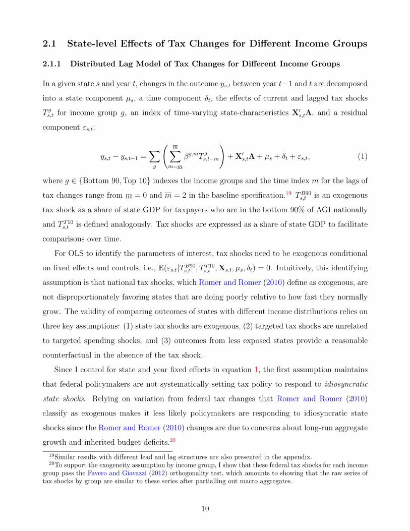
In a given state s and year t, changes in the outcome ys,t between year t−1 and t are decomposed

into a state component µs, a time component δt, the effects of current and lagged tax shocks

T gs,t for income group g, an index of time-varying state-characteristics X′s,tΛ, and a residual

component εs,t:

ys,t − ys,t−1 =∑g

(m∑

m=m

βg,mT gs,t−m

)+ X′s,tΛ + µs + δt + εs,t, (1)

where g ∈ {Bottom 90,Top 10} indexes the income groups and the time index m for the lags of

tax changes range from m = 0 and m = 2 in the baseline specification.19 TB90s,t is an exogenous

tax shock as a share of state GDP for taxpayers who are in the bottom 90% of AGI nationally

and T T10s,t is defined analogously. Tax shocks are expressed as a share of state GDP to facilitate

comparisons over time.

For OLS to identify the parameters of interest, tax shocks need to be exogenous conditional

on fixed effects and controls, i.e., E(εs,t|TB90s,t , T T10

s,t ,Xs,t, µs, δt) = 0. Intuitively, this identifying

assumption is that national tax shocks, which Romer and Romer (2010) define as exogenous, are

not disproportionately favoring states that are doing poorly relative to how fast they normally

grow. The validity of comparing outcomes of states with different income distributions relies on

three key assumptions: (1) state tax shocks are exogenous, (2) targeted tax shocks are unrelated

to targeted spending shocks, and (3) outcomes from less exposed states provide a reasonable

counterfactual in the absence of the tax shock.

Since I control for state and year fixed effects in equation 1, the first assumption maintains

that federal policymakers are not systematically setting tax policy to respond to idiosyncratic

state shocks. Relying on variation from federal tax changes that Romer and Romer (2010)

classify as exogenous makes it less likely policymakers are responding to idiosyncratic state

shocks since the Romer and Romer (2010) changes are due to concerns about long-run aggregate

growth and inherited budget deficits.20

19Similar results with different lead and lag structures are also presented in the appendix.20To support the exogeneity assumption by income group, I show that these federal tax shocks for each income

group pass the Favero and Giavazzi (2012) orthogonality test, which amounts to showing that the raw series oftax shocks by group are similar to these series after partialling out macro aggregates.

10

Even if state tax shocks are exogenous, they may occur at the same time as other progressive

policy changes. If progressive tax and spending policy systematically occur at the same time

and both increase growth, then βB90 would reflect both the true effect of tax changes for the

bottom 90% and the effects of spending policies, resulting in upwardly-biased estimates. To

address this concern, I directly control for government transfer payments as well as specific

policy parameters. I first control for a comprehensive measure of total government spending

on transfer programs, but this amount of spending responds to economic conditions. To isolate

changes in policy parameters from changes in economic conditions, my preferred approach is to

control for mechanical policy-induced changes in social insurance program spending. I include

the mechanical policy-induced spending changes of several key transfer programs in the vector of

controls Xs,t in the baseline specification, and then present estimates that control for additional

policy parameters in robustness specifications.

I provide several pieces of evidence to support the third assumption that outcomes from

less exposed states provide a reasonable counterfactual in the absence of the tax shock. I

consider the possibility that states that disproportionately benefit from a given tax change

may be generally more cyclical. I do so by replacing year fixed effects δt in equation 1 with

δq(s),t where δq(s),t is each state’s cyclicality-quintile-specific year fixed effect. The function

q(s) : {AL,AK, ...,WY } → {1, ..., 5} gives the quintile of the state’s sensitivity to national

changes in economic conditions. I present a few ways to measure how cyclically-sensitive each

state is, but the baseline approach follows the β-differencing approach of Blanchard and Katz

(1992), which regresses changes in state economic activity on national changes in economic

activity to estimate the state’s average responsiveness to national shocks.21 The resulting group-

by-year fixed effect δq(s),t measures common year shocks in the 10 states with similar levels

of cyclicality. Additionally, I consider regional trends as well as other controls used in the

regional multiplier literature (e.g., state-specific trends and state-specific interest rate and oil

price sensitivity). I provide further support for the third assumption by examining the path of

economic activity preceding tax shocks for bottom- and top-income groups.

21See appendix B.1 for details. I also show results using deciles instead of quintiles and using quintiles ofeach state’s standard deviation in real GDP per capita σs,1963−1979 in the years preceding the sample period1980-2007.

11

2.1.2 Direct Projections of Tax Changes for Different Income Groups

To examine how the path of economic activity evolves before and after tax shocks for bottom-

and top-income groups, I run a series of direct projection regressions for different horizons

h ∈ {−4,−3, ..., 5}:

ys,t+h − ys,t−1 = αB90h (TB90

s,t ) + αT10h (T T10

s,t ) + X′s,tΛh + µs,h + δt,h + εs,t,h, (2)

where s and t index state and year, ys,t+h − ys,t−1 is a measure of growth in economic activity

at horizon h, and µs,h and δt,h are horizon-specific state and year fixed effects.22 The path

of economic activity around the tax shocks for bottom and top-income groups is described by

the sequences of coefficients {αB90h }h=5

h=−4 and {αT10h }h=5

h=−4, which quantify the impacts of these

shocks on economic activity over different horizons. As noted by Jorda (2005); Stock and

Watson (2007); Auerbach and Gorodnichenko (2013), using direct projections of tax shocks

on outcomes is attractive because it does not impose dynamic restrictions on the estimates at

different horizons. I use these specifications to estimate average outcomes before tax shocks to

determine if tax shocks for different groups occur soon after unusually good or bad economic

times. The direct projection approach also shows how the effects of tax changes vary over time

and can potentially reveal anticipatory effects, which may vary by income group.

2.1.3 Two-Year Effects of Tax Changes for Different Income Groups

While the direct projection specifications are useful for examining how economic activity evolves

around a tax change, I fit more parsimonious models that use two-year changes to show the

cumulative effects of tax changes on employment and income for different income groups.23 The

two-year specification follows a similar specification to Nakamura and Steinsson (2014), but for

tax shocks (by income group) rather than for government spending shocks:

22In the baseline specification, I use cyclicality-quintile year fixed effects described in the prior section, i.e.,δq(s),t formed using the β-differencing approach of Blanchard and Katz (1992), which are indexed by the horizon,i.e., δq(s),t,h. I also include the mechanical policy-induced spending changes of several key transfer programs inthe vector of controls Xs,t in the baseline specification as well. Specifically, the 5 distinct policy controls are themechanical changes in AFDC, TANF, SNAP, SSI, and Medicaid spending as a percentage of state GDP.

23Note that each of the elements of the tax shock are normalized by the initial level of state GDP (i.e., Ys,t−2).There is nothing special about two-year changes per se other than that this duration is somewhat standard inthis literature (e.g., Nakamura and Steinsson (2014)).

12

Ys,t − Ys,t−2Ys,t−2

= bB90

(2∑

m=0

TB90s,t−m

)+ bT10

(2∑

m=0

T T10s,t−m

)+ X′s,tΛ + as + dt + es,t. (3)

In this case, the year fixed effects dt absorb common aggregate macroeconomic shocks and the

state-fixed effects effectively control for different state trends in the outcome. An advantage of

this specification is that the average effects of tax changes are captured by one parameter for

each income group (rather than a parameter for each lag of each income group). I use dq(s),t

instead of dt in the baseline specification (where dq(s),t is each state’s cyclicality-quintile-specific

year fixed effect) and also control for mechanical policy-induced spending changes.

2.2 National Effects of Tax Changes for Different Income Groups

I also fit specifications similar to equation 1 at the national level:

yt − yt−1 =m∑

m=m

(γB90,mTB90

t−m + γT10,mT T10t−m + X′t−mΓm

)+ νt, (4)

where γB90,m and γT10,m are the effects of changes in taxes as a share of GDP at lag m and

the time index m for the lags of tax changes range from m = 0 and m = 2 in the baseline

specification. TB90t is an exogenous tax shock as a share of national GDP for taxpayers who

are in the bottom 90% of AGI nationally and T T10t is defined analogously. Xt = [TNONINC,t]

includes non-income and non-payroll tax changes that Romer and Romer (2010) classify as

exogenous (e.g., corporate tax changes). One way to interpret equation 4 is that it decomposes

the Romer and Romer (2010) exogenous tax change measure into three mutually exclusive and

collectively exhaustive components: TB90t , T T10

t , and the non-income and non-payroll portion,

i.e., TNONINC,t.

3 Effect of Tax Changes for Different Income Groups

This section provides results on the effects of tax changes for different income groups on economic

activity. Section 3.1 provides evidence on the effects of tax changes for different groups on

employment and income growth. Section 3.2 provides results for mechanisms and highlights

supplemental national results. Section 3.3 discusses the estimates and relates them to existing

13

evidence. Finally, section 3.4 briefly describes additional support for the validity of the estimates

and robustness tests.

3.1 Impacts on State Economic Activity

Figure 3 shows the evolution of the state employment-to-population ratio and state employment

relative to the year before a tax change for different income groups. Panel A shows that the

employment-to-population ratio exhibits little trend prior to tax changes and then gradually

falls in the years following a tax change for the bottom 90%. Specifically, the estimates for

the impact of tax changes in year h for the bottom 90%, αB90h from equation 2, and those

for the top 10%, αT10h , are shown in blue and red respectively. The employment-to-population

ratio is roughly 4 percentage points lower three years after a 1% of state GDP tax change for

the bottom 90% relative to the employment-to-population ratio the year before the tax change

(i.e., αB903 ≈ 4). After four years, on average, the ratio improves slightly to be roughly 3

percentage points below the level prior to the tax change. Panel B shows similar patterns for

state employment. State employment tends to be 2% lower in the year after the tax change

for the bottom 90%, falls to 4% two years after the change, and then recovers somewhat to be

roughly 2% lower four years after the tax change. Tax changes for the top 10%, in contrast,

have no detectable impact on the state employment-to-population ratio and state employment

in the eight-year window around tax changes.

Figure 4 shows the evolution of the state income and prices. Panel A shows that nominal

state GDP sharply declines following tax changes for the bottom 90% and is roughly 8 percent

lower than the year before the tax change. These declines are very large.24 However, panel B

shows prices also fall by roughly 6 percent. This price decline estimate is noisy, but indicates

that the GDP declines are smaller in real terms. Panels C and D show results for real GDP

using the ACCRA price index PACCRAs,t and a home-price-based index PHPI

s,t . The real series

show smaller impacts, especially three and four years after the tax changes for the bottom 90%.

In terms of estimates from tax changes for the top 10%, estimates for both measures of income in

nominal and real terms provide no evidence that tax changes for high-income earners materially

impact economic activity over a business cycle frequency.25

24I discuss the magnitudes and relate them to existing literature in section 3.3.25While it is possible that the effects show up further into the future, detecting such effects is inherently

difficult. See Romer and Romer (2014) for some historical evidence on longer-term effects.

14

Table 1 presents the main regression estimates of state employment and income. Panel

A shows estimates of the distributed lag specification using equation 1 as well as the sum of

effects∑2

m=0 βg,m of tax changes for each group g ∈ {Bottom 90,Top 10}. Panel B shows

estimates from the more parsimonious two-year change specification using 3. For each panel,

the baseline specification is a rich set of controls: mechanical policy changes in spending as a

share of state GDP on social insurance programs (AFDC, TANF, SNAP, SSI, and Medicaid) as

well as state and cyclicality-quintile by year fixed effects. Employment declines roughly 3.5% in

both specifications following a tax change of 1% of state GDP for the bottom 90%, and top tax

changes have no impact in either specification. Panel B also reports the p-value for the test that

bB90 = bB90, i.e., that the impacts on two-year employment growth from tax changes for both

groups are equal. This test is rejected with 94% confidence in column 1. The employment-to-

population ratio also shows similar patterns but is less precise over a two-year window relative

to three and four years after the tax change as shown in Figure 3. The next three columns

show estimates for nominal and real state GDP. The impacts are very large for the bottom

90% and not for the top 10%. Although the point estimates for state GDP are less stable and

range from 5.3% to 9.2%, the qualitative pattern of nearly all responsiveness from lower-income

groups and small impacts from top groups is very robust.26 Each specification rejects the null

hypothesis of equal impacts from tax changes for the bottom 90% and top 10% with more than

99% confidence.

3.2 Mechanisms

The results in section 3.1 show large employment and income declines after tax changes affecting

lower-income taxpayers. These employment and income results are reduced-form estimates that

reflect changes in both the supply and demand for labor following a tax change. This section

discusses impacts on labor market outcomes and on consumption, the relative importance of

supply and demand changes at the state level, and effects on aggregate investment.

Figure 5 shows the impacts of tax changes for different groups on extensive and intensive

labor market responses, real wages, and consumption. On the extensive margin, Panel A shows

that labor force participation rates decline roughly 3 percentage points three and four years

26Appendix Tables A8 and A9 show robustness tests for nominal state GDP. Appendix Tables A10 and A11show robustness tests for real state GDP.

15

after a tax change for the bottom 90%. On the intensive margin, hours of workers who work

at least 48 weeks decline by roughly 2 percent soon after the tax change but return to the

levels before the tax change.27 Panel C shows that real wages increase following tax changes for

the bottom 90%.28 These real wage results, though imprecise, reveal the relative importance

of supply and demand changes in the labor market. The increase in real wages suggests that

supply-side responses are important and may exceed demand-side responses to tax changes for

the bottom 90%.

In terms of aggregate mechanisms, Table 4 shows national results for real GDP and its

components. Real GDP decreases 3.8% following tax changes for the bottom 90% and decreases

1.1% following tax changes for the top 10%. These point estimates are noisy – the standard error

for the top 10% estimate is 4.6% at the national level – but could be consistent with impacts

of tax changes from the top 10% that spillover to other states. That said, the impacts on the

top 10% are statistically indistinguishable from zero and 2.7 percentage points lower than the

aggregate estimate for the bottom 90%. The components of GDP are also noisy.29 Other than

the impacts on investment, which are much more responsive to tax changes for the bottom 90%

and are weakly significant statistically, there is not enough variation in the time series to pin

down heterogeneous effects on macro aggregates.30 The investment responses and the overall

real GDP point estimates, however, suggest that the effects of additional economic growth from

tax changes for the bottom 90% tend to exceed the effects from income changes among those

who are more likely to save.

27Results are similar for hours of workers who work on average at least 35 hours per week and at least 48weeks per year.

28Nominal wages tend to be roughly flat but then increase following tax changes for the bottom 90%. PanelC uses the ACCRA price index PACCRA

s,t as a deflator and adjusts wages holding constant the composition ofworkers, which indicates that the real wage increases are reflecting actual increases rather than compositionalshifts in labor supply. Results using other deflators and raw average wages are similar and presented in appendixFigure A14.

29Given the limited number of tax changes events in the postwar period, the possibility of coincidental trendsin income inequality, for example, suggests caution when interpreting the national results and provides anotherreason why evidence from the state-level analysis, especially when the analysis accounts for regional trends, maybe more informative.

30The consumption results are somewhat mixed. Although durable good consumption is much more responsiveto bottom 90% tax changes, the non-durable consumption estimates work in the opposite direction, leading tosimilar overall consumption impacts. The similarity in consumption impacts is inconsistent with the literatureon MPCs and the state-level results in Figure 4 which show much larger responses from the bottom 90% onconsumption.

16

3.3 Discussion of Results

Quantitatively, the main reduced-form results in this paper are large, but within a range that is

consistent with existing cross-sectional evidence. In particular, the 3.4% estimate for the increase

in state employment from a 1% of GDP tax cut for the bottom 90% translates to roughly $31,500

per job.31 These cost-per-job estimates are consistent with those reported in Ramey (2011):

$25,000 in Wilson (2012), roughly $28, 600 in Chodorow-Reich et al. (2012), $30,000 in Suarez

Serrato and Wingender (2011), and $35,000 in Shoag (2010).32 My estimates for the impact

of tax cuts for the top 10% on employment are statistically and economically indistinguishable

from zero, so the corresponding cost-per-job estimate is much higher. Therefore, given my

estimates by income group, the overall impact of a tax cut of 1% of GDP that goes half to the

bottom 90% and half to the top 10% will have roughly a $63,000 cost-per-job.

The estimates for impacts on real income, however, are larger than most papers in this

literature.33 First, the variation that I am exploiting could potentially yield stronger effects than

prior studies. Second, the confidence intervals are large, so one cannot rule out smaller effects.

Third, in terms of point estimates, the average output multiplier in a recent survey by Chodorow-

Reich (2017) is 2.1, though some studies estimate sizable cumulative output multipliers (e.g.,

Leduc and Wilson (2015) estimate a cumulative multiplier of 6.6). The estimated impact on real

income from the bottom 90% depends on the specification, but is roughly 7.34 The impact from

the top 10% is roughly zero, so the overall multiplier on real income, computed as the average of

the group-specific multipliers, is roughly 3.5. It is important to emphasize that these estimates

are regional multipliers, which can differ from national multipliers to the extent that time fixed

effects absorb general equilibrium forces (e.g., countercyclical monetary policy).35 Since state

31Using 2011 numbers, the cost of a 1% of GDP tax cut is roughly $150 billion and a 3.4% increase inemployment on a base of 140 million is 4.76 million. Therefore, the cost-per-job is $150,000M

4.76M = $31, 513.32Note that Wilson (2012) and Chodorow-Reich et al. (2012) focus on effects during a recession, which likely

results in lower cost-per-job estimates. There are also estimates of smaller multipliers (e.g., Clemens and Miran(2012)). See Chodorow-Reich (2017) for a recent survey.

33Nakamura and Steinsson (2014), for example, find output multipliers from government spending of 1.32 to4.79 in their Table 3 and roughly similar estimates for output multipliers in real terms.

34See, for example, Figure 4 panels C and D or the real income estimates in Table 1 or appendix Tables A6and A7. Other measures of income, e.g., total personal income from CPS, increase by roughly 5% as shown inappendix Figure A21, but these estimates are noisy.

35Although regional multipliers are generally believed to be larger than national multipliers, the relative sizeof regional and national multipliers is an active area of research (Chodorow-Reich, 2017). It is also worth notingthat common national shocks like countercyclical monetary policy are not likely to be fully absorbed by time fixedeffects given regional heterogeneity and the possibility of heterogeneous impacts of monetary policy changes.

17

GDP, particularly in real terms, is measured with error,36 my preferred interpretation of these

results is that the point estimates for real income are more variable and thus less reliable than the

employment estimates, but impacts on both outcomes provide robust evidence that economic

activity is substantially more responsive to tax changes for the bottom 90% than to those for

the top 10%. Okun’s law suggests that employment and GDP are closely related, so putting

emphasis on the better measured of the two seems advantageous.

In terms of mechanisms and the relative importance of consumption and labor supply re-

sponses, rationalizing the large responses in economic activity through consumption responses

alone is not persuasive. First, the traditional multiplier of MPC1−MPC

would require marginal

propensities to consume that are larger than most MPCs estimated in the literature, e.g., John-

son et al. (2006) and Parker et al. (2013). Second, in terms of heterogeneous MPCs by income

group, the initial impact on consumption could be sizable,37 but the subsequent rounds do not

feed back exclusively to lower-income groups, so the MPCs in subsequent rounds are not the

MPCs of lower-income consumers, but economy-wide average MPCs. Third, to the extent some

of the initial spending is on durable goods, which are often traded, the impacts from increased

consumption may not be especially concentrated in the states where tax change recipients live

(other than through spillovers to the consumption of complementary non-tradables). Substan-

tial labor supply responses, therefore, are likely an important mechanism, which is consistent

with the evidence presented on labor force participation, hours, and real wages.

One may find these results surprising from the perspective of the theoretical literature.

Although the employment estimates are comparable to those in the empirical literature on

regional multipliers, it may be somewhat surprising from the perspective of the theoretical

literature that tax cuts for lower-income earners are more effective than government spending.38

Farhi and Werning (2016), however, show that externally-financed regional multipliers with

36BEA relies on measures from a range of sources when computing state GDP, many of which are from theeconomic census. The economic census is compiled every five years and in non-benchmark years, state GDPestimates involve “interpolation and extrapolation techniques using indicator series that mirror the movement inthe GDP by state component being estimated.” See https://www.bea.gov/regional/pdf/gsp/GDPState.pdf.

37 Aaronson et al. (2012) show that household spending increases by roughly $700 per quarter following a$250 per quarter income increase due to minimum wage increases. This 700

250 ≈ 3X impact on spending amonglow-income earners comes from a small number of households that make large durable purchases following theincome shock. Similar spending behavior following tax shocks for lower-income earners could generate sizableimpacts on economic activity.

38MPC estimates are typically smaller than 1 and the traditional government spending multiplier is 11−MPC ,

so the traditional tax multiplier is smaller than the traditional government spending multiplier, i.e., MPC < 1implies that MPC

1−MPC < 11−MPC .

18

https://www.bea.gov/regional/pdf/gsp/GDPState.pdf

redistribution and non-Ricardian agents can be larger than traditional multipliers. Additionally,

other channels, such as extensive margin labor supply responses with heterogeneous agents, are

often not incorporated and can impact conclusions about multipliers.

The results may also be surprising in terms of Ricardian equivalence. Ricardian agents

will increase expenditures based on the annuity value of the tax change, which may be zero

if they expect to finance the tax change in the future.39 However, there are a few reasons

why Ricardian equivalence may fail, especially when considering tax changes for lower-income

groups in a spatial setting. First, agents may consider tax changes a transfer if the tax change

is (i) financed contemporaneously by other agents (from other locations or from other income

groups) or (ii) if they expect others to pay for it in the future. Second, agents may be liquidity

constrained. Third, agents may be myopic. These considerations may also help explain why

there are different impacts for different income groups.

3.4 Threats to Validity and Robustness

There are three key threats to the validity of the estimates: endogenous tax changes, prior

economic conditions and differential trends, and concomitant progressive government spending

changes. First, I assess the concern that the composition of tax shocks may be endogenous by

appealing to an orthogonality test used by Favero and Giavazzi (2012). This test compares the

federal tax change series before and after partialling out macro aggregates. Appendix Figure A8

shows that the raw tax shock series and the orthogonalized tax shock series are very similar for

each income group, supporting the compositional exogeneity assumption.40

Tables 2 and 3 present distributed lag estimates for a wide range of robustness tests to

address the second and third concerns, respectively. Table 2 shows impacts of tax changes on

state employment growth.41 The first five columns present different ways to account for state-

specific cyclicality; (1) presents the baseline specification with cyclicality-quintile by year fixed

effects, (2) presents year effects, (3) presents cyclicality-quintile by year fixed effects where the

39This discussion of Ricardian equivalence draws from the discussion of Ricardian equivalence and regionalmultipliers in Chodorow-Reich (2017).

40More generally, tax changes could be endogenous by income group, year, and state. I address concerns withrespect to the timing and location of tax changes by using only tax changes Romer and Romer (2010) classifyas exogenous and by exploiting regional variation in the income distribution.

41Appendix Tables A8 and A9 show results for nominal state GDP. Appendix Tables A10 and A11 showresults for real state GDP.

19

quintiles are defined based on the standard deviation in state GDP per capita, (4) cyclicality-

decile by year fixed effects, and (5) cyclicality-quintile by year fixed effects that group states

only using the years before the sample (i.e., before 1980). The next five columns show controls

for state-specific sensitivity to other shocks and trends; (6) controls for oil price interacted with

state dummies, (7) controls for real interest rate interacted with state dummies, (8) and (9)

add region fixed effects to (6) and (7), and (10) includes state-specific trends. The specific

point estimates for the impact on employment growth from tax changes for the bottom 90%

depend on the specification, are almost always significant statistically, and tend to be within a

one percentage point range of the baseline estimates. Similar patterns emerge in Table 3, which

shows results for a wide range of policy parameters and controls for government spending. Panel

B of both tables show the same controls using the two-year change specification for additional

measures of economic activity and show similar patterns. For example, Table 3 shows that

two-year employment growth following a tax change for the bottom 90% ranges between 3.2

percent to 3.6 percent across 11 different policy controls. Overall, the general patterns are quite

robust. Almost all the impact on economic activity from tax changes comes from tax changes

from the bottom 90%.

4 Conclusion

This paper quantifies the importance of the distribution of tax changes for their overall impact

on economic activity. I construct a new data series of tax changes by income group from tax

return data. I use this series and variation from the income distribution across states and

federal tax shocks to estimate the effects of tax changes for different groups. I find that the

stimulative effects of income tax cuts are largely driven by tax cuts for the bottom 90% and

that the empirical link between employment growth and tax changes for the top 10% is weak

to negligible over a business cycle frequency. These effects are not confounded by changes in

progressive spending, state trends, or prior economic conditions. The effects seem to come from

labor supply responses as well as increased consumption and investment.

These results are important for characterizing central equity-efficiency tradeoffs in tax policy.

If policy makers aim to increase economic activity in the short to medium run, this paper

strongly suggests that tax cuts for top-income earners will be less effective than tax cuts for

20

lower-income earners. While it is possible that tax cuts for top-income earners have sizable

long-run impacts through different channels such as human capital investment, firm creation,

or innovation,42 much more compelling evidence on these channels is needed to support top-

income tax cuts on efficiency grounds, especially given the magnitude of resources devoted to

these tax policy changes. Overall, the results not only suggest some skepticism for “trickle

down” economics, but they also provide evidence that supply-side tax policies should do more

to consider the relative efficacy of tax cuts targeted lower in the income distribution. Finally, as

a note of caution, the estimates in this paper come from modest changes in tax rates that have

been executed in the post-war period; using these estimates to evaluate the likely impacts of

large tax changes on high-income earners requires extrapolation beyond the observed variation

in the data.

42Extending the analysis to study medium- and longer-term effects of tax changes, such as new firm creationor patent activity, is a good topic for future research.

21

References

Aaronson, Daniel, Sumit Agarwal, and Eric French, “The Spending and Debt Responseto Minimum Wage Hikes,” American Economic Review, 2012, 102 (7), 3111–3139.

Auerbach, Alan and Jonathan Siegel, “Capital-Gains Realizations of the Rich and Sophis-ticated,” American Economic Review, 2000, 90 (2), 276–282.

Auerbach, Alan J. and Yuriy Gorodnichenko, “Output Spillovers from Fiscal Policy,”American Economic Review, May 2013, 103 (3), 141–46.

Autor, David H., Alan Manning, and Christopher L. Smith, “The Contribution of theMinimum Wage to US Wage Inequality over Three Decades: A Reassessment,” AmericanEconomic Journal: Applied Economics, January 2016, 8 (1), 58–99.

Barro, Robert J. and Charles J. Redlick, “Macroeconomic Effects from Government Pur-chases and Taxes,” The Quarterly Journal of Economics, 2011, 126 (1), 51–102.

Blanchard, Olivier Jean and Lawrence F. Katz, “Regional Evolutions,” Brookings Paperson Economic Activity, 1992, 1992 (1), 1–75.

Busso, Matias, Jesse Gregory, and Patrick Kline, “Assessing the Incidence and Efficiencyof a Prominent Place Based Policy,” American Economic Review, September 2013, 103 (2),897–947.

Chetty, Raj, John N. Friedman, Sren Leth-Petersen, Torben Heien Nielsen, andTore Olsen, “Active vs. Passive Decisions and Crowd-Out in Retirement Savings Accounts:Evidence from Denmark,” The Quarterly Journal of Economics, 2014, 129 (3), 1141–1219.

Chodorow-Reich, Gabriel, “Geographic Cross-Sectional Fiscal Multipliers: What Have WeLearned?,” Harvard University Working Paper, 2017.

, Laura Feiveson, Zachary Liscow, and William Gui Woolston, “Does State FiscalRelief During Recessions Increase Employment? Evidence from the American Recovery andReinvestment Act,” American Economic Journal: Economic Policy, 2012, 4 (3), 118–145.

Clemens, Jeffrey and Stephen Miran, “Fiscal Policy Multipliers on Subnational Govern-ment Spending,” American Economic Journal: Economic Policy, 2012, 4 (2), 46–68.

Dynan, Karen, Jonathan Skinner, and Stephen Zeldes, “Do the Rich Save More?,”Journal of Political Economy, 2004, 112 (2), 397–444.

Eissa, Nada and Jeffrey B. Liebman, “Labor Supply Response to the Earned Income TaxCredit,” The Quarterly Journal of Economics, 1996, 111 (2), 605–637.

Farhi, Emmanuel and Ivan Werning, “Fiscal Multipliers: Liquidity Traps and CurrencyUnions,” Handbook of Macroeconomics, forthcoming, 2016, 2, 2417–2492.

Favero, Carlo and Francesco Giavazzi, “Measuring Tax Multipliers: The Narrative Methodin Fiscal VARs,” American Economic Journal: Economic Policy, 2012, 4 (2), 69–94.

22

Frisch, Ragnar and Frederick V. Waugh, “Partial Time Regressions as Compared withIndividual Trends,” Econometrica, 1933, 1 (4), 387–401.

Galı, Jordi, J. David Lopez-Salido, and Javier Valles, “Understanding the Effects ofGovernment Spending on Consumption,” Journal of the European Economic Association,2007, 5 (1), 227–270.

Goolsbee, Austan, “What Happens When You Tax the Rich? Evidence from ExecutiveCompensation,” Journal of Political Economy, 2000, 108 (2), 352–378.

Hausman, Joshua K., “Fiscal Policy and Economic Recovery: The Case of the 1936 Veterans’Bonus,” American Economic Review, 2016, 106 (4), 1100–1143.

Heathcote, Jonathan, “Fiscal Policy with Heterogenous Agents and Incomplete Markets,”Review of Economic Studies, 2005, 72 (1), 161–188.

Heckman, James J., “Comment,” in “Behavioral Simulation Methods in Tax Policy Analy-sis,” University of Chicago Press, 1983, pp. 70–82.

Jappelli, Tullio and Luigi Pistaferri, “The Consumption Response to Income Changes,”Annual Review of Economics, 2010, 2, 479–506.

Johnson, David S., Jonathan A. Parker, and Nicholas S. Souleles, “Household Ex-penditure and the Income Tax Rebates of 2001,” American Economic Review, 2006, 96 (5),1589–1610.

Jorda, Oscar, “Estimation and Inference of Impulse Responses by Local Projections,” Amer-ican Economic Review, 2005, 95 (1), 161–182.

Kline, Patrick and Melissa Tartari, “Bounding the Labor Supply Responses to a Random-ized Welfare Experiment: A Revealed Preference Approach,” American Economic Review,2016, 106 (4), 972–1014.

Kosar, Gizem and Robert A. Moffitt, “Trends in Cumulative Marginal Tax Rates Fac-ing Low-Income Families, 1997-2007,” Working Paper 22782, National Bureau of EconomicResearch 2016.

Leduc, Sylvain and Daniel Wilson, “Are State Governments Roadblocks to Federal Stim-ulus? Evidence from Highway Grants in the 2009 Recovery Act,” Federal Reserve Bank ofSan Francisco Working Paper, 2015.

McCarthy, Jonathan, “Imperfect Insurance and Differing Propensities to Consume AcrossHouseholds,” Journal of Monetary Economics, 1995, 36 (2), 301–327.

Mertens, Karel, “Marginal Tax Rates and Income: New Time Series Evidence,” NBER Work-ing Paper 19171, 2013.

and Morten O. Ravn, “The Dynamic Effects of Personal and Corporate Income TaxChanges in the United States,” American Economic Review, 2013, 103 (4), 1212–1247.

and , “A Reconciliation of SVAR and Narrative Estimates of Tax Multipliers,” Journalof Monetary Economics, 2014, 68, S1–S19.

23

Meyer, Bruce and Dan T. Rosenbaum, “Welfare, the Earned Income Tax Credit, andthe Labor Supply of Single Mothers,” The Quarterly Journal of Economics, 2001, 116 (3),1063–1114.

Monacelli, Tommaso and Roberto Perotti, “Tax Cuts, Redistribution, and BorrowingConstraints,” Technical Report, Bocconi University May 2011.

Moretti, Enrico, “Real Wage Inequality,” American Economic Journal: Applied Economics,2013, 5 (1), 65–103.

Nakamura, Emi and Jon Steinsson, “Fiscal Stimulus in a Monetary Union: Evidence fromUS Regions,” American Economic Review, 2014, 104 (3), 753–792.

Parker, Jonathan, “The Reaction of Household Consumption to Predictable Changes in SocialSecurity Taxes,” American Economic Review, 1999, 89 (4), 959–973.

Parker, Jonathan A., Nicholas S. Souleles, David S. Johnson, and Robert Mc-Clelland, “Consumer Spending and the Economic Stimulus Payments of 2008,” AmericanEconomic Review, 2013, 103 (6), 2530–2553.

Ramey, Valerie A., “Can Government Purchases Stimulate the Economy?,” Journal of Eco-nomic Literature, 2011, 49 (3), 673–685.

Romer, Christina D. and David H. Romer, “The Macroeconomic Effects of Tax Changes:Estimates Based on a New Measure of Fiscal Shocks,” American Economic Review, 2010, 100(3), 763–801.

and , “The Incentive Effects of Marginal Tax Rates: Evidence from the Interwar Era,”American Economic Journal: Economic Policy, 2014, 6 (3), 242–281.

Ruggles, Steven, Katie Genadek, Ronald Goeken, Josiah Grover, and MatthewSobek, “Integrated Public Use Microdata Series: Version 5.0 [dataset],” Minneapolis: Uni-versity of Minnesota 2010.

Saez, Emmanuel, “Do Taxpayers Bunch at Kink Points?,” American Economic Journal:Economic Policy, 2010, 2 (3), 180–212.

and Gabriel Zucman, “Wealth Inequality in the United States since 1913: Evidence fromCapitalized Income Tax Data,” The Quarterly Journal of Economics, 2016, 131 (2), 519–578.

, Joel Slemrod, and Seth H. Giertz, “The Elasticity of Taxable Income with Respect toMarginal Tax Rates: A Critical Review,” Journal of Economic Literature, 2012, 50 (1), 3–50.

Serrato, Juan Carlos Suarez and Owen Zidar, “Who Benefits from State Corporate TaxCuts? A Local Labor Markets Approach with Heterogeneous Firms,” American EconomicReview, 2016, 106 (9), 2582–2624.

Shapiro, Matthew D. and Joel Slemrod, “Consumer Response to the Timing of Income:Evidence from a Change in Tax Withholding,” American Economic Review, March 1995, 85(1), 274–283.

24

Shoag, Daniel, “The Impact of Government Spending Shocks: Evidence on the Multiplierfrom State Pension Plan Returns,” Working Paper, Harvard University 2010.

Stock, James and Mark Watson, “Why has U.S. Inflation Become Harder to Forcast?,”Journal of Money, Banking and Credit, 2007, 39, 3–33.

Suarez Serrato, Juan Carlos and Philippe Wingender, “Estimating Local Fiscal Multi-pliers,” Working Paper, U.C. Berkeley 2011.

Wilson, Daniel J., “Fiscal Spending Jobs Multipliers: Evidence from the 2009 AmericanRecovery and Reinvestment Act,” American Economic Journal: Economic Policy, 2012, 4(3), 251–282.

Yagan, Danny, “Is the Great Recession Really Over? Longitudinal Evidence of EnduringEmployment Impacts,” Unpublished Manuscript, 2016.

25

Figure 1: Selected Historical Tax Changes for Each AGI Percentile

−2

02

−2

02

0 50 100 0 50 100

1982 1991

1993 2003

Ave

rag

e C

ha

ng

e in

Ta

x L

iab

ility

as S

ha

re o

f A

GI

AGI PercentileGraphs by Year

Notes: This figure displays the average mechanical change in income and payroll tax liability for each tax return in TAXSIM from tax schedule changes as

a share of adjusted gross income (AGI) by AGI percentile for 1993 and for three other prominent years. For display purposes, it does not show results for

the smallest AGI percentile (since the smallest income group result is amplified by a small denominator).

Figure 2: Federal Tax Changes by Income Group and Heterogeneous High-Income Shares

A. Federal Income and Payroll Tax Changes by AGI Quintile

-.6-.4

-.20

.2.4

.6Pe

rcen

t of G

DP

1950 1960 1970 1980 1990 2000 2010Year

Tax Change: Bottom 20% Tax Change: 21-40%Tax Change: 41-60% Tax Change: 61-80%Tax Change: Top 20% Exogenous Changes

B. Share of High-Income Taxpayers

11.47 − 15.489.92 − 11.478.66 − 9.927.57 − 8.666.84 − 7.573.90 − 6.84

Notes: This figure shows that there is both time-series and cross-sectional variation in tax changes by income

group. Panel A displays changes in individual income and payroll tax liabilities by income quintile as a share of

GDP from 1950 to 2007. Tax returns from TAXSIM are used to construct a tax change measure. The period

from 2008-2011 has no exogenous tax changes so those years are coded as zero exogenous change for each AGI

quintile throughout the paper. Both exogenous and endogenous tax changes are shown in the figure (Appendix

Table A1 shows how each tax change is classified). Panel B shows that there is substantial geographic variation

in the location of households in the top-income decile. For instance, 12.4% of households filing from Virginia

are in the top 10% of AGI nationally on average from 1980-2007. The data plotted are the average shares of

households filing from a given state for the years 1980-2007 who are in the top 10% nationally in that year.

Figure 3: Cumulative Growth in State Employment-to-Population Ratio and Employment

A. Employment-to-Population Ratio B. Employment

-.1-.0

50

.05

Per

cent

age

poin

ts

-3 -2 -1 0 1 2 3 4Years Since Tax Change

Bottom 90 Top 10

-.1-.0

50

.05

Per

cent


Bottom 90 Top 10

Notes: This figure shows event studies of a 1% of GDP tax increase on the state employment-to-population ratio and employment for those with AGI inthe bottom 90% nationally in blue and for those with AGI in the top 10% nationally in red. Specifically, the figure plots the estimates from the baselinespecification of equation 2 for the impact of tax changes in year h for the bottom 90%, αB90

h , and the top 10%, αT10h . The baseline specification includes

controls for mechanical changes in AFDC, TANF, SNAP, SSI, and Medicaid spending as a percentage of state GDP, as well as cyclicality-quintile year fixedeffects. See section 2 for details. Standard errors are robust and clustered by state; 95% confidence intervals are shown as dotted lines. The sample periodis 1980-2007.

28

Figure 4: Cumulative Growth in State Economic Activity

-.15

-.1-.0

50

.05

.1P

erce

nt


A. Nominal GDP

-.15

-.1-.0

50

.05

.1P

erce

nt


B. ACCRA Price Index

-.2-.1

0.1

.2P

erce

nt


C. Real GDP (ACCRA)

-.15

-.1-.0

50

.05

.1P

erce

nt


D. Real GDP (Moretti HPI)

Bottom 90 Top 10

Notes: This figure shows event studies of a 1% of GDP tax increase on outcomes for those with AGI in the bottom 90% nationally in blue and for those withAGI in the top 10% nationally in red. These outcomes are (a) nominal state GDP, (b) the ACCRA state price index PACCRA

s,t , (c) real state GDP using

PACCRAs,t , and (d) real state GDP using PMoretti

s,t . Specifically, the figure plots the estimates from the baseline specification of equation 2 for the impact

of tax changes in year h for the bottom 90%, αB90h , and the top 10%, αT10

h . The baseline specification includes controls for mechanical changes in AFDC,TANF, SNAP, SSI, and Medicaid spending as a percentage of state GDP, as well as cyclicality-quintile year fixed effects. See section 2 for details. Standarderrors are robust and clustered by state; 95% confidence intervals are shown as dotted lines. The sample period is 1980-2007.

29

Figure 5: Cumulative Growth in State Labor Market Outcomes and Consumption

-.1-.0

50

.05

Perc

enta

ge p

oint

s


A. Labor Force Participation Rate

-.04

-.02

0.0

2.0

4Pe

rcen

t


B. Hours

-.2-.1

0.1

.2Pe

rcen

t


C. Composition-Constant Real Wages (ACCRA)

-.15

-.1-.0

50

.05

.1Pe

rcen

t


D. Consumption

Bottom 90 Top 10

Notes: This figure shows event studies of a 1% of GDP tax increase on outcomes for those with AGI in the bottom 90% nationally in blue and for those withAGI in the top 10% nationally in red. These outcomes are (a) labor force participation rate (in percentage points), (b) mean hours worked among thosethat have worked at least 48 weeks in the past year, (c) real composition-constant average wages using PACCRA

s,t , and (d) state consumption. Specifically,

the figure plots the estimates from the baseline specification of equation 2 for the impact of tax changes in year h for the bottom 90%, αB90h , and the top

10%, αT10h . The baseline specification includes controls for mechanical changes in AFDC, TANF, SNAP, SSI, and Medicaid spending as a percentage of

state GDP, as well as cyclicality-quintile year fixed effects. See section 2 for details. Standard errors are robust and clustered by state; 95% confidenceintervals are shown as dotted lines. The sample period is 1980-2007 for (a)-(c). However, state consumption is only available since 1997, so the sampleperiod for (d) is 1997-2007.

30

Table 1: State-level Effects of Tax Changes for Different Income Groups

Panel A: Distributed Lag Model of Tax Changes for Different Income GroupsEmployment Emp/Pop Nominal GDP Real GDP (ACCRA) Real GDP (Moretti)

B90 0.33 0.97 -2.05 -0.29 0.86(1.22) (1.59) (2.18) (2.83) (2.79)

B90 1-Year Lag -1.87** -1.23 -7.39*** -8.40*** -5.96***(0.89) (1.34) (1.34) (2.85) (1.87)

B90 2-Year Lag -1.98 -2.48* 0.25 2.11 -0.17(1.25) (1.35) (1.44) (2.11) (2.05)

T10 0.52 0.47 1.05* 0.91 1.00(0.45) (0.40) (0.58) (0.99) (1.08)

T10 1-Year Lag -0.24 -0.66 0.10 0.88 -0.11(0.60) (0.41) (0.70) (0.61) (1.25)

T10 2-Year Lag -0.61 -0.80 -0.12 -0.12 -0.41B90 Sum: βt + βt−1 + βt−2 -3.52 -2.74 -9.19*** -6.59 -5.27

(2.28) (1.68) (3.40) (4.97) (4.44)T10 Sum: βt + βt−1 + βt−2 -0.33 -0.99 1.03 1.67 0.48

(1.57) (0.65) (1.56) (1.33) (3.41)Bottom - Top: -3.19 -1.74 -10.22** -8.26 -5.75

(3.14) (1.87) (3.96) (5.10) (4.57)

Panel B: Two-Year ChangesEmployment Emp/Pop Nominal GDP Real GDP (ACCRA) Real GDP (Moretti)

Bottom 90 -3.42** -1.53 -11.98*** -9.70*** -7.00**(1.54) (0.96) (2.21) (3.46) (2.88)

Top 10 0.22 -0.24 0.75 1.44* 0.56(0.90) (0.33) (0.96) (0.85) (2.17)

P-Value (Bottom 90 = Top 10) 0.06 0.23 0.00 0.00 0.03

Notes: Panel A presents estimates of the effects of tax changes for different income groups g ∈{Bottom 90,Top 10} at different lags m from the following specification: ys,t − ys,t−1 = αs + δq(s),t +∑

g

(∑2m=0 β

g,mT gs,t−m

)+X′s,tΛ+εs,t, where ys,t is the log outcome (for all outcomes other than the employment-

to-population ratio, which is measured in percentage terms), αs is a state-fixed effect, δq(s),t is each state’scyclicality-quintile-specific year fixed effect where q(s) : {AL,AK, ...,WY } → {1, ..., 5} to be the quintile ofthe state’s sensitivity to national changes in economic conditions (see section 2.1.1 or appendix B.1 for de-tails), TB90

s,t is an exogenous tax shock as a share of state GDP for taxpayers who are in the bottom 90%

of AGI nationally, TT10s,t is defined analogously, and Xs,t includes controls for mechanical changes in AFDC,

TANF, SNAP, SSI, and Medicaid spending as a percentage of state GDP with the same lag structure as thetax changes (i.e., current values, one year lags, and two year lags). Similarly, Panel B presents estimates ofthe effects of tax changes for the bottom 90%, bB90, and the top 10%, bT10, from the following specification:Ys,t−Ys,t−2

Ys,t−2= as + dq(s),t + bB90

(∑2m=0 T

B90s,t−m

)+ bT10

(∑2m=0 T

T10s,t−m

)+ X′s,tΛ + es,t, where Ys,t is the level

of the outcome,Ys,t−Ys,t−2

Ys,t−2is two-year growth in the outcome, as is a state-fixed effect, dq(s),t is each state’s

cyclicality-quintile-specific year fixed effect,(∑2

m=0 Tgs,t−m

)is the change in taxes over the last two years, and

Xs,t includes controls for mechanical changes in AFDC, TANF, SNAP, SSI, and Medicaid spending as a shareof state GDP defined analogously as the tax shocks. For the Employment-to-Population ratio, the outcome isthe simple difference, i.e., Ys,t − Ys,t−2. P-values for the null hypothesis that the effects of tax changes for thebottom 90% and top 10% are the same, i.e., bB90 = bT10, are presented in the last row of Panel B. Standarderrors are clustered by state (*** p<0.01, ** p<0.05, * p<0.1). Data are at the state-year level from 1980-2007.See appendix A.2 for data definitions and sources.

31

Table 2: State-level Effects of Tax Changes by Income Group on Employment: Cyclical Robustness(1) (2) (3) (4) (5) (6) (7) (8) (9) (10) (11) (12)

Panel A: Distributed Lag Model of Tax Changes for Different Income GroupsTB90s,t 0.33 1.01 0.40 0.36 1.22 0.89 0.40 1.10 0.44 -0.17 -0.33 -0.50

(1.22) (0.87) (0.72) (1.26) (0.93) (0.90) (0.78) (1.10) (1.03) (1.23) (1.42) (1.29)TB90s,t−1 -1.87** -2.07** -1.71** -1.91** -1.41* -2.14** -2.27*** -1.98** -2.37*** -2.22** -2.41*** -2.49**

(0.89) (0.78) (0.67) (0.78) (0.76) (0.81) (0.76) (0.82) (0.65) (1.00) (0.70) (1.00)TB90s,t−2 -1.98 -1.17 -0.86 -2.24* -0.85 -1.32 -1.84* -1.19 -1.86* -2.80* -2.84* -2.58*

(1.25) (1.10) (0.87) (1.19) (1.22) (1.18) (1.03) (1.33) (0.93) (1.43) (1.42) (1.35)T T10s,t 0.52 0.33 0.22 0.32 0.32 0.29 0.32 0.33 0.29 0.56 0.55 0.48

(0.45) (0.32) (0.32) (0.36) (0.28) (0.32) (0.32) (0.36) (0.36) (0.46) (0.44) (0.48)T T10s,t−1 -0.24 -0.43 -0.19 -0.56 -0.30 -0.49 -0.55 -0.38 -0.55 -0.28 -0.26 -0.29

(0.60) (0.44) (0.46) (0.50) (0.36) (0.46) (0.46) (0.39) (0.43) (0.65) (0.55) (0.63)T T10s,t−2 -0.61 -0.66 -0.59 -0.92 -0.62 -0.74 -0.83* -0.58 -0.82* -0.74 -0.69 -0.67

(0.67) (0.46) (0.56) (0.56) (0.42) (0.47) (0.49) (0.36) (0.42) (0.72) (0.62) (0.69)B90 Sum: βt + βt−1 + βt−2 -3.52 -2.23 -2.17 -3.80** -1.04 -2.57 -3.71** -2.06 -3.79** -5.20** -5.58** -5.57**

(2.28) (2.07) (1.81) (1.87) (2.11) (2.22) (1.71) (2.60) (1.66) (2.52) (2.05) (2.73)T10 Sum: βt + βt−1 + βt−2 -0.33 -0.76 -0.56 -1.17 -0.60 -0.94 -1.06 -0.62 -1.08 -0.46 -0.40 -0.48

(1.57) (1.07) (1.17) (1.21) (0.85) (1.08) (1.10) (0.81) (0.96) (1.67) (1.34) (1.65)Bottom - Top: -3.19 -1.47 -1.61 -2.63 -0.44 -1.63 -2.64 -1.43 -2.71 -4.74 -5.18* -5.10

(3.14) (2.13) (2.43) (2.36) (2.06) (2.26) (2.17) (2.73) (2.02) (3.48) (2.78) (3.63)

Panel B: Two-Year ChangesBottom 90 -3.42** -2.58* -2.58* -3.58*** -1.55 -2.68* -3.45*** -2.45 -3.37** -4.25** -4.44** -4.69**

(1.54) (1.31) (1.33) (1.28) (1.35) (1.38) (1.16) (1.77) (1.35) (1.71) (1.57) (1.80)Top 10 0.22 -0.00 -0.05 -0.24 -0.01 -0.02 -0.11 0.10 -0.14 0.31 0.24 0.15

(0.90) (0.65) (0.61) (0.66) (0.49) (0.63) (0.59) (0.54) (0.57) (0.88) (0.72) (0.93)P-Value (Bottom 90 = Top 10) 0.06 0.04 0.12 0.02 0.22 0.04 0.01 0.20 0.06 0.03 0.04 0.03

Controls1) Baseline Cyclicality Y N N N N N N N N Y Y Y2) Year N Y N N N Y Y Y Y N N N3) σGDPPC Cyclicality N N Y N N N N N N N N N4) Alternate β-diff Control #1 N N N Y N N N N N N N N5) Alternate β-diff Control #2 N N N N Y N N N N N N N6) Oil Price x State N N N N N Y N N N Y N N7) Real Interest Rate x State N N N N N N Y N N Y N N8) Oil Price x State + Region Y N N N N N N Y N N Y N9) Real Interest Rate x State + Region N N N N N N N N Y N Y N10) State Trends N N N N N N N N N N N Y

Notes: Each specification is the same as column 1 in Table 1 other than the controls. The first five columns present different ways to account for state-specificcyclicality (see section 2.1.1 or appendix B.1 for details); (1) baseline specification with cyclicality-quintile by year fixed effects, (2) year fixed effects, (3)cyclicality-quintile by year fixed effects where the quintiles are defined based on the standard deviation in state GDP per capita, (4) cyclicality-decile byyear fixed effects, and (5) cyclicality-quintile by year fixed effects that group states only using the years before the sample (i.e., before 1980). The nextfive columns show controls for state-specific sensitivity to other shocks and trends; (6) controls for oil price interacted with state dummies, (7) controls forreal interest rate interacted with state dummies, (8) and (9) add region fixed effects to (6) and (7), and (10) includes state-specific trends. Standard errorsare clustered by state (*** p<0.01, ** p<0.05, * p<0.1) in all specifications other than (8) and (9), which are clustered by region. The sample period is1980-2007. See appendix A.2 for data definitions and sources.

32

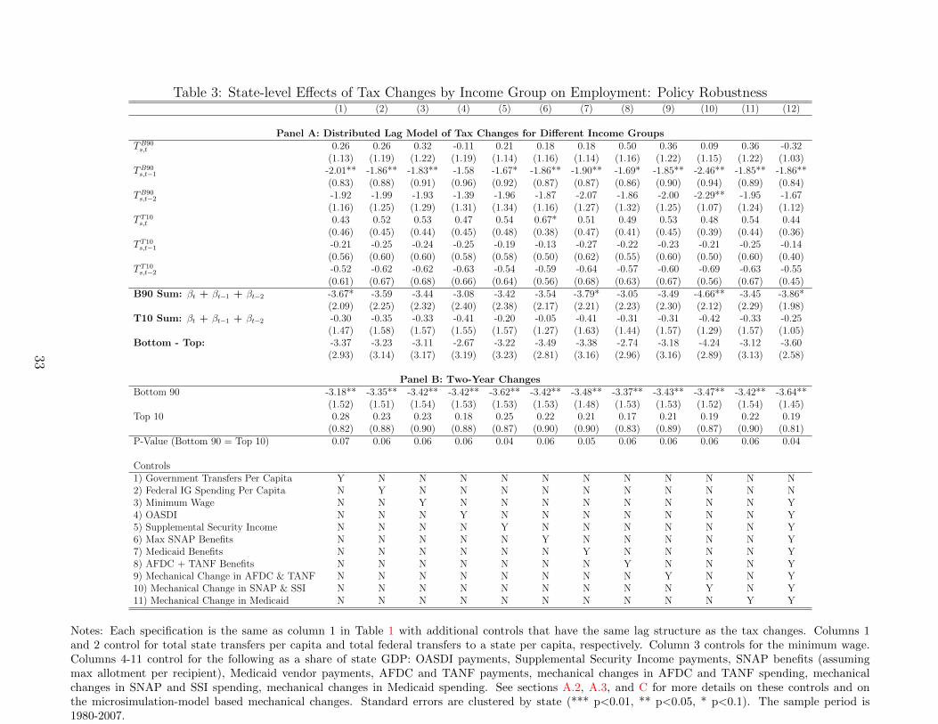
Table 3: State-level Effects of Tax Changes by Income Group on Employment: Policy Robustness(1) (2) (3) (4) (5) (6) (7) (8) (9) (10) (11) (12)

Panel A: Distributed Lag Model of Tax Changes for Different Income GroupsTB90s,t 0.26 0.26 0.32 -0.11 0.21 0.18 0.18 0.50 0.36 0.09 0.36 -0.32

(1.13) (1.19) (1.22) (1.19) (1.14) (1.16) (1.14) (1.16) (1.22) (1.15) (1.22) (1.03)TB90s,t−1 -2.01** -1.86** -1.83** -1.58 -1.67* -1.86** -1.90** -1.69* -1.85** -2.46** -1.85** -1.86**

(0.83) (0.88) (0.91) (0.96) (0.92) (0.87) (0.87) (0.86) (0.90) (0.94) (0.89) (0.84)TB90s,t−2 -1.92 -1.99 -1.93 -1.39 -1.96 -1.87 -2.07 -1.86 -2.00 -2.29** -1.95 -1.67

(1.16) (1.25) (1.29) (1.31) (1.34) (1.16) (1.27) (1.32) (1.25) (1.07) (1.24) (1.12)T T10s,t 0.43 0.52 0.53 0.47 0.54 0.67* 0.51 0.49 0.53 0.48 0.54 0.44

(0.46) (0.45) (0.44) (0.45) (0.48) (0.38) (0.47) (0.41) (0.45) (0.39) (0.44) (0.36)T T10s,t−1 -0.21 -0.25 -0.24 -0.25 -0.19 -0.13 -0.27 -0.22 -0.23 -0.21 -0.25 -0.14

(0.56) (0.60) (0.60) (0.58) (0.58) (0.50) (0.62) (0.55) (0.60) (0.50) (0.60) (0.40)T T10s,t−2 -0.52 -0.62 -0.62 -0.63 -0.54 -0.59 -0.64 -0.57 -0.60 -0.69 -0.63 -0.55

(0.61) (0.67) (0.68) (0.66) (0.64) (0.56) (0.68) (0.63) (0.67) (0.56) (0.67) (0.45)B90 Sum: βt + βt−1 + βt−2 -3.67* -3.59 -3.44 -3.08 -3.42 -3.54 -3.79* -3.05 -3.49 -4.66** -3.45 -3.86*

(2.09) (2.25) (2.32) (2.40) (2.38) (2.17) (2.21) (2.23) (2.30) (2.12) (2.29) (1.98)T10 Sum: βt + βt−1 + βt−2 -0.30 -0.35 -0.33 -0.41 -0.20 -0.05 -0.41 -0.31 -0.31 -0.42 -0.33 -0.25

(1.47) (1.58) (1.57) (1.55) (1.57) (1.27) (1.63) (1.44) (1.57) (1.29) (1.57) (1.05)Bottom - Top: -3.37 -3.23 -3.11 -2.67 -3.22 -3.49 -3.38 -2.74 -3.18 -4.24 -3.12 -3.60

(2.93) (3.14) (3.17) (3.19) (3.23) (2.81) (3.16) (2.96) (3.16) (2.89) (3.13) (2.58)

Panel B: Two-Year ChangesBottom 90 -3.18** -3.35** -3.42** -3.42** -3.62** -3.42** -3.48** -3.37** -3.43** -3.47** -3.42** -3.64**

(1.52) (1.51) (1.54) (1.53) (1.53) (1.53) (1.48) (1.53) (1.53) (1.52) (1.54) (1.45)Top 10 0.28 0.23 0.23 0.18 0.25 0.22 0.21 0.17 0.21 0.19 0.22 0.19


Controls1) Government Transfers Per Capita Y N N N N N N N N N N N2) Federal IG Spending Per Capita N Y N N N N N N N N N N3) Minimum Wage N N Y N N N N N N N N Y4) OASDI N N N Y N N N N N N N Y5) Supplemental Security Income N N N N Y N N N N N N Y6) Max SNAP Benefits N N N N N Y N N N N N Y7) Medicaid Benefits N N N N N N Y N N N N Y8) AFDC + TANF Benefits N N N N N N N Y N N N Y9) Mechanical Change in AFDC & TANF N N N N N N N N Y N N Y10) Mechanical Change in SNAP & SSI N N N N N N N N N Y N Y11) Mechanical Change in Medicaid N N N N N N N N N N Y Y

Notes: Each specification is the same as column 1 in Table 1 with additional controls that have the same lag structure as the tax changes. Columns 1and 2 control for total state transfers per capita and total federal transfers to a state per capita, respectively. Column 3 controls for the minimum wage.Columns 4-11 control for the following as a share of state GDP: OASDI payments, Supplemental Security Income payments, SNAP benefits (assumingmax allotment per recipient), Medicaid vendor payments, AFDC and TANF payments, mechanical changes in AFDC and TANF spending, mechanicalchanges in SNAP and SSI spending, mechanical changes in Medicaid spending. See sections A.2, A.3, and C for more details on these controls and onthe microsimulation-model based mechanical changes. Standard errors are clustered by state (*** p<0.01, ** p<0.05, * p<0.1). The sample period is1980-2007.

33

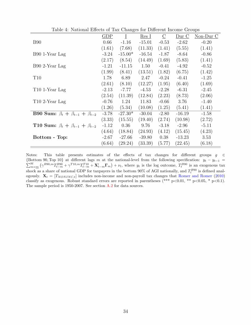
Table 4: National Effects of Tax Changes for Different Income Groups

GDP I Res I C Dur C Non-Dur CB90 0.66 -1.16 -15.01 -0.53 -2.62 -0.20

(1.61) (7.68) (11.33) (1.41) (5.55) (1.41)B90 1-Year Lag -3.24 -15.00* -16.54 -1.87 -8.64 -0.86

(2.17) (8.54) (14.49) (1.69) (5.83) (1.41)B90 2-Year Lag -1.21 -11.15 1.50 -0.41 -4.92 -0.52

(1.99) (8.41) (13.51) (1.82) (6.75) (1.42)T10 1.78 6.89 2.47 -0.24 -0.41 -1.25

(2.61) (8.10) (12.27) (1.95) (6.40) (1.69)T10 1-Year Lag -2.13 -7.77 -4.53 -2.28 -6.31 -2.45

(2.54) (11.39) (12.84) (2.23) (8.73) (2.06)T10 2-Year Lag -0.76 1.24 11.83 -0.66 3.76 -1.40

(1.26) (5.34) (10.08) (1.25) (5.41) (1.41)B90 Sum: βt + βt−1 + βt−2 -3.78 -27.30* -30.04 -2.80 -16.19 -1.58

(3.33) (15.55) (19.40) (2.74) (10.98) (2.72)T10 Sum: βt + βt−1 + βt−2 -1.12 0.36 9.76 -3.18 -2.96 -5.11

(4.64) (18.84) (24.93) (4.12) (15.45) (4.23)Bottom - Top: -2.67 -27.66 -39.80 0.38 -13.23 3.53

(6.64) (29.24) (33.39) (5.77) (22.45) (6.18)

Notes: This table presents estimates of the effects of tax changes for different groups g ∈{Bottom 90,Top 10} at different lags m at the national-level from the following specification: yt − yt−1 =∑m

m=m

(γB90,mTB90

t−m + γT10,mTT10t−m + X′t−mΓm

)+ νt, where yt is the log outcome, TB90

t is an exogenous tax

shock as a share of national GDP for taxpayers in the bottom 90% of AGI nationally, and TB90t is defined anal-

ogously. Xt = [TNONINC,t] includes non-income and non-payroll tax changes that Romer and Romer (2010)classify as exogenous. Robust standard errors are reported in parentheses (*** p<0.01, ** p<0.05, * p<0.1).The sample period is 1950-2007. See section A.2 for data sources.

34

Appendices for Online Publication

This appendix contains several sections. Section A.1 discusses how I measure tax changes

in the years before NBER’s TAXSIM is available. It also enumerates all of the tax changes

and how they are classified. Section A.2 defines all economic variables used in the paper and

documents sources. Similarly, section A.3 defines and provides sources for all of the policy and

social insurance variables. Section B describes how I construct adjustments for state-specific

cyclicality, namely, how I construct β-differencing cyclicality groups. Section C describes the

social insurance microsimulation models and how they are used to estimate annual state-specific

policy-induced changes in social insurance spending.

A Data

A.1 Tax Data

35

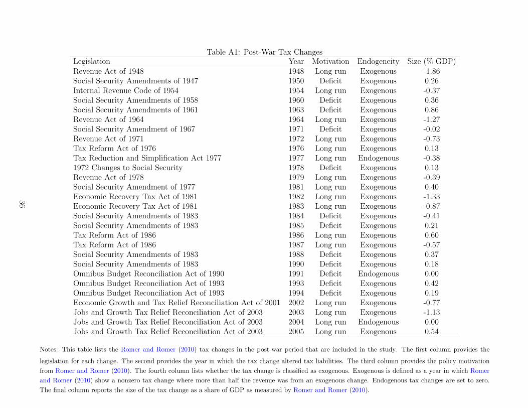
Table A1: Post-War Tax ChangesLegislation Year Motivation Endogeneity Size (% GDP)Revenue Act of 1948 1948 Long run Exogenous -1.86Social Security Amendments of 1947 1950 Deficit Exogenous 0.26Internal Revenue Code of 1954 1954 Long run Exogenous -0.37Social Security Amendments of 1958 1960 Deficit Exogenous 0.36Social Security Amendments of 1961 1963 Deficit Exogenous 0.86Revenue Act of 1964 1964 Long run Exogenous -1.27Social Security Amendment of 1967 1971 Deficit Exogenous -0.02Revenue Act of 1971 1972 Long run Exogenous -0.73Tax Reform Act of 1976 1976 Long run Exogenous 0.13Tax Reduction and Simplification Act 1977 1977 Long run Endogenous -0.381972 Changes to Social Security 1978 Deficit Exogenous 0.13Revenue Act of 1978 1979 Long run Exogenous -0.39Social Security Amendment of 1977 1981 Long run Exogenous 0.40Economic Recovery Tax Act of 1981 1982 Long run Exogenous -1.33Economic Recovery Tax Act of 1981 1983 Long run Exogenous -0.87Social Security Amendments of 1983 1984 Deficit Exogenous -0.41Social Security Amendments of 1983 1985 Deficit Exogenous 0.21Tax Reform Act of 1986 1986 Long run Exogenous 0.60Tax Reform Act of 1986 1987 Long run Exogenous -0.57Social Security Amendments of 1983 1988 Deficit Exogenous 0.37Social Security Amendments of 1983 1990 Deficit Exogenous 0.18Omnibus Budget Reconciliation Act of 1990 1991 Deficit Endogenous 0.00Omnibus Budget Reconciliation Act of 1993 1993 Deficit Exogenous 0.42Omnibus Budget Reconciliation Act of 1993 1994 Deficit Exogenous 0.19Economic Growth and Tax Relief Reconciliation Act of 2001 2002 Long run Exogenous -0.77Jobs and Growth Tax Relief Reconciliation Act of 2003 2003 Long run Exogenous -1.13Jobs and Growth Tax Relief Reconciliation Act of 2003 2004 Long run Endogenous 0.00Jobs and Growth Tax Relief Reconciliation Act of 2003 2005 Long run Exogenous 0.54

Notes: This table lists the Romer and Romer (2010) tax changes in the post-war period that are included in the study. The first column provides the

legislation for each change. The second provides the year in which the tax change altered tax liabilities. The third column provides the policy motivation

from Romer and Romer (2010). The fourth column lists whether the tax change is classified as exogenous. Exogenous is defined as a year in which Romer

and Romer (2010) show a nonzero tax change where more than half the revenue was from an exogenous change. Endogenous tax changes are set to zero.

The final column reports the size of the tax change as a share of GDP as measured by Romer and Romer (2010).

36

A.1.1 Pre-NBER Tax Changes

Only four exogenous changes, affecting tax liabilities in 1948, 1950, 1954, and 1960, took place in

a time preceding the coverage of TAXSIM. For each of these changes, I manually calculated tax

changes by income group using the SOI data.43 The SOI reports provide data on the number

of taxable returns and the amount of taxable income for groups created by size of adjusted

gross income. With many AGI brackets, one can form a rough idea of how taxes changed

across the income distribution. For each income bracket, I created a representative taxpayer

by dividing the amount of taxable income by the number of taxable returns. I then calculated

this representative person’s change in payroll or federal income tax liability using her income

in the year prior to the tax change, the old schedule and the new schedule. Data from the tax

schedule were from (2) and (3) for the income tax changes and from (5) for the payroll rate and

base changes. For instance, in 1960, any representative taxpayer whose earnings were below the

payroll tax base of $4,800 had to pay 1% of their income extra since rates increased from 5%

to 6%. Note that Barrow and Sahasakul (1983) used a somewhat similar approach to calculate

average marginal rates.

In general, the following sources were helpful for constructing these tax change measures: (1)

the Brooking Institution’s “Individual Income Tax Brackets, 1945-2010,” (2) the Tax Founda-

tion’s “U.S. Federal Individual Income Tax Rates History, 1913-2010,” (3) the Internal Revenue

Service’s annual individual income tax return reports, and (4) the Tax Policy Center’s Historical

Payroll Tax Rates report.44

A.1.2 Tax Change Calculation for Each Tax Return: 1993 Example

This section provides an example of the tax liability change calculation described in 1.1.1 for

1993. Recall the 1993 Omnibus Budget Reconciliation Act, which raised rates on high-income

taxpayers by adding new brackets in 1993 according to the schedule in Table A2. For every

taxpayer, my measure subtracts how much she paid in 1992 from how much she would have paid

in 1992 if the 1993 tax schedule had been in place. Figure A6 plots the results for 1993.45 Many

individuals with adjusted gross income above $100,000, and especially those with adjusted gross

income exceeding $150,000, faced a roughly thousand-dollar tax increase based on this measure.

43 The 1948 change was from the Revenue Act of 1948, the 1950 change was from the 1947 Social SecurityAmendment, the 1954 change was from the 1950 Social Security Amendment and the Internal Revenue Code of1954, and the 1960 change was from the 1958 Social Security Amendment (Romer & Romer (2009)).

44Note that the Tax Policy Center data on the payroll base and rates come from the following two SocialSecurity Administration sites: http://www.ssa.gov/OACT/COLA/cbb.html and http://www.ssa.gov/OACT/

ProgData/taxRates.html.45Note that the 1993 results are based on the sample of 1992 tax returns and the 1992 and 1993 tax schedules.

37

http://www.ssa.gov/OACT/COLA/cbb.html

http://www.ssa.gov/OACT/ProgData/taxRates.html

http://www.ssa.gov/OACT/ProgData/taxRates.html

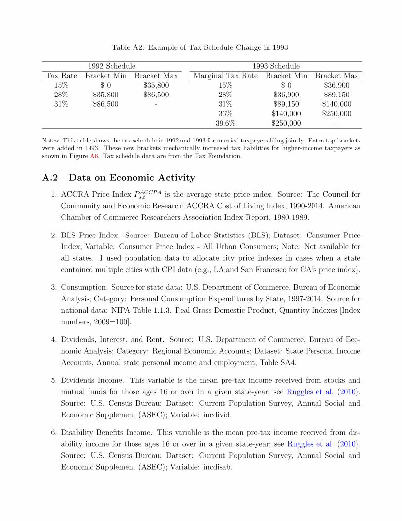
Table A2: Example of Tax Schedule Change in 1993

1992 Schedule 1993 ScheduleTax Rate Bracket Min Bracket Max Marginal Tax Rate Bracket Min Bracket Max

15% $ 0 $35,800 15% $ 0 $36,90028% $35,800 $86,500 28% $36,900 $89,15031% $86,500 - 31% $89,150 $140,000

36% $140,000 $250,00039.6% $250,000 -

Notes: This table shows the tax schedule in 1992 and 1993 for married taxpayers filing jointly. Extra top bracketswere added in 1993. These new brackets mechanically increased tax liabilities for higher-income taxpayers asshown in Figure A6. Tax schedule data are from the Tax Foundation.

A.2 Data on Economic Activity

1. ACCRA Price Index PACCRAs,t is the average state price index. Source: The Council for

Community and Economic Research; ACCRA Cost of Living Index, 1990-2014. American

Chamber of Commerce Researchers Association Index Report, 1980-1989.

2. BLS Price Index. Source: Bureau of Labor Statistics (BLS); Dataset: Consumer Price

Index; Variable: Consumer Price Index - All Urban Consumers; Note: Not available for

all states. I used population data to allocate city price indexes in cases when a state

contained multiple cities with CPI data (e.g., LA and San Francisco for CA’s price index).

3. Consumption. Source for state data: U.S. Department of Commerce, Bureau of Economic

Analysis; Category: Personal Consumption Expenditures by State, 1997-2014. Source for

national data: NIPA Table 1.1.3. Real Gross Domestic Product, Quantity Indexes [Index

numbers, 2009=100].

4. Dividends, Interest, and Rent. Source: U.S. Department of Commerce, Bureau of Eco-

nomic Analysis; Category: Regional Economic Accounts; Dataset: State Personal Income

Accounts, Annual state personal income and employment, Table SA4.

5. Dividends Income. This variable is the mean pre-tax income received from stocks and

mutual funds for those ages 16 or over in a given state-year; see Ruggles et al. (2010).

Source: U.S. Census Bureau; Dataset: Current Population Survey, Annual Social and

Economic Supplement (ASEC); Variable: incdivid.

6. Disability Benefits Income. This variable is the mean pre-tax income received from dis-

ability income for those ages 16 or over in a given state-year; see Ruggles et al. (2010).


Economic Supplement (ASEC); Variable: incdisab.

7. Durable Consumption. Source: NIPA Table 1.1.3. Real Gross Domestic Product, Quan-

tity Indexes [Index numbers, 2009=100].

8. Employment: This variable indicates the number of people employed in a given state-year.

Source: Bureau of Labor Statistics, Local Area Unemployment Statistics.

9. Employment Rate. This variable is the share of people, ages 16 or over, in the labor force

who report employment status 10 “At work” or 12 “Has job, not at work last week” in the

CPS; see Ruggles et al. (2010). Source: U.S. Census Bureau; Dataset: Current Population

Survey, Annual Social and Economic Supplement (ASEC).

10. Employment-to-Population Ratio. This variable is the share of people, ages 16 or over,

who report employment status 10 “At work” or 12 “Has job, not at work last week” in the

CPS; see Ruggles et al. (2010). Source: U.S. Census Bureau; Dataset: Current Population


11. FHFA HPI Index. This is a broad measure of the movement of single-family house prices.

It measures the average price changes in repeat sales or refinancing on the same properties.

Source: Federal Housing Finance Agency House Price Index Datasets, Purchase-Only

Indexes (Estimated using Sales Price Data).

12. GDP. Source: NIPA Table 1.1.3. Real Gross Domestic Product, Quantity Indexes [Index

numbers, 2009=100].

13. Hours. This variable is the mean hours worked by employed residents in a given state-year

given that they worked at least 48 weeks that year and are at least 16 years of age. This

variable is constructed using data drawn from the U.S. Census Bureau; Dataset: Current

Population Survey, Annual Social and Economic Supplement (ASEC); see Ruggles et al.

(2010). I follow Moretti (2013) by restricting the sample to workers aged between 25

and 60 and by using uhrsworkly, wkswork1, and wkswork2 to create a proxy for the

number of weeks worked by taking the mean value of wkswork2 in cases where wkswork1

is missing, and call this proxy wkswork. Hours is the product of wkswork and uhrsworkly.

I additionally restrict the sample to those who work at least 48 weeks (as determined by

the proxy wkswork, described above).

14. Interest Income. This variable is the mean pre-tax income received from interest on savings

accounts, certificates of deposit, money market funds, bonds, treasury notes, IRAs, and/or

other investments which paid interest for those ages 16 or over in a given state-year; see

Ruggles et al. (2010). Source: U.S. Census Bureau; Dataset: Current Population Survey,

Annual Social and Economic Supplement (ASEC); Variable: incint.

15. Investment. Source: NIPA Table 1.1.3. Real Gross Domestic Product, Quantity Indexes

[Index numbers, 2009=100].

39

16. Labor Force Participation Rate. This variable is the share of persons, ages 16 or over,

participating in the labor force; see Ruggles et al. (2010). Source: U.S. Census Bureau;

Dataset: Current Population Survey, Annual Social and Economic Supplement (ASEC).

This variable is constructed simply from the given indicator “labforce,” which is an in-

dicator for whether that person is in the labor force. Those coded “yes” were either: at

work; held a job but were temporarily absent due to factors like vacation or illness; seeking

work; or were temporarily laid off during the reference period.

17. Moretti CPI Price Index PCPIs,t . This variable is a state-specific price index that is con-

structed following Moretti (2013):

(a) I draw gross monthly rental cost of housing (rentgrs) from the Current Population


(b) Housing consumption weights wt are provided by Moretti (2013)& Yagan (2016).

These weights estimate the portion of non-housing costs that vary systematically

with housing costs. For reference, this weight is approximately .35 in 2000.

(c) Define ps,t as average gross monthly rental cost of housing by state-year.

(d) Define rs,1980 the average gross monthly rental cost of housing by state in 1980.

(e) Define cpit as national CPI from FRED, anchored to 1 in 1980.

(f) Define rental CPI cpirs,t=ps,trs,1980

. Let cpirt be the annual mean of cpirs,t.

(g) Then define cpiadjt =cpit

(1− wt)− wt

(1− wt)cpirt .

(h) Finally, let PCPIs,t = (1− wt)(cpi

adjt ) + w(cpirs,t).

As noted in Moretti (2013), this measure includes local variation in housing and non-

housing costs, but is limited in that non-housing costs come from national cpi and so that

portion of the price index does not vary by state.

18. Moretti HPI Price Index PMorettis,t . This variable is a state-specific price index that is

constructed following Moretti (2013). The construction of this variable follows the same

steps as “Moretti CPI” above, except I utilize a Housing Price Index (FHFA HPI Index)

in place of rentgrs. HPI is drawn from Federal Housing Finance Agency House Price

Index Datasets, Purchase-Only Indexes (Estimated using Sales Price Data). See FHFA

HPI Index above for a short description of this variable.

19. Net Earnings. Source: U.S. Department of Commerce, Bureau of Economic Analysis; Cat-

egory: Regional Economic Accounts; Dataset: State Personal Income Accounts, Annual

state personal income and employment, Table SA4.

20. Nominal GDP. Source: NIPA Table 1.1.5.

40

21. Oil Price. This variable is the average spot price of West Texas Intermediate. Source: St.

Louis Federal Reserve FRED database.

22. Part-time Employment Rate. This variable is the share of persons, ages 16 or over,

participating in the labor force who report employment status 10 “At work” or 12 “Has

job, not at work last week” in the CPS, and also worked fewer than 48 weeks in the past

year. I use wkswork1 and wkswork2 to create a proxy for the number of weeks worked

by taking the mean value of wkswork2 in cases where wkswork1 is missing. Each of these

variable is drawn from the CPS; see Ruggles et al. (2010). Source: U.S. Census Bureau;

Dataset: Current Population Survey, Annual Social and Economic Supplement (ASEC).

23. Payroll. This variable is the total state payroll in a given year. Source: Quarterly Census

of Employment and Wages (QCEW) - Statewide.

24. Personal Income. Source: U.S. Department of Commerce, Bureau of Economic Analy-

sis; Category: Regional Economic Accounts; Dataset: State Personal Income Accounts,

Annual state personal income and employment, Table SA4.

25. Personal Transfer Receipts. Source: U.S. Department of Commerce, Bureau of Economic

Analysis; Category: Regional Economic Accounts; Dataset: State Personal Income Ac-

counts, Annual state personal income and employment, Table SA4.

26. Real Interest Rate. This variable is generated through the Federal Funds Rate less national

CPI inflation. Source: St. Louis Federal Reserve FRED database.

27. Rent Income. This variable is the mean pre-tax income received from rent (after ex-

penses) for those ages 16 or over in a given state-year; see Ruggles et al. (2010). Source:

U.S. Census Bureau; Dataset: Current Population Survey, Annual Social and Economic

Supplement (ASEC); Variable: incrent.

28. Residential Investment. Source: NIPA Table 1.1.3. Real Gross Domestic Product, Quan-

tity Indexes [Index numbers, 2009=100].

29. State GDP. This variable indicates the Gross Domestic Product by state-year. Source:

U.S. Department of Commerce, Bureau of Economic Analysis; Category: Regional Eco-

nomic Accounts; Dataset: Annual Gross Domestic Product (GDP) by State; Series: SIC

All GDP Components & NAICS All GDP Components.

30. State Population. This variable indicates the number of residents in a state-year. Source:

Federal Reserve Bank of St. Louis, FRED; Series: Resident Population in state s.

31. State GDP/Capita. This variable is state GDP divided by State Population; sources

above.

41

32. Total Income. This variable is the mean total pre-tax personal income or losses from all

sources for those ages 16 or over in a given state-year; see Ruggles et al. (2010). Source:


Supplement (ASEC); Variable: inctot.

33. Unemployment Benefit Income. This variable is the mean pre-tax income received from

state or federal unemployment compensation, Supplemental Unemployment Benefits (SUB),

or union unemployment or strike benefits for those ages 16 or over in a given state-year.


Economic Supplement (ASEC); Variable: incunemp.

34. Wage. This variable is the mean wage of full-time workers in a given state-year. This

is built utilizing variables from the U.S. Census Bureau; Dataset: Current Population

Survey, Annual Social and Economic Supplement (ASEC); see Ruggles et al. (2010). I

follow Moretti (2013) in terms of sample restrictions. Specifically, I take wage to be

incwage/hours, where incwage comes directly from the CPS and hours is constructed as

noted in the item above. In cases in which workers work fewer than 48 weeks per year,

as estimated by the wkswork proxy also noted above, I set the wage value to missing so

that the state-year measure reflects the average wages of full-time workers as in Moretti

(2013). Finally, I restrict the sample to workers aged between 25 and 60.

35. Welfare Income. This variable is the mean pre-tax income received from various public

assistant programs (welfare) for those ages 16 or over in a given state-year; see Ruggles

et al. (2010). Source: U.S. Census Bureau; Dataset: Current Population Survey, Annual

Social and Economic Supplement (ASEC); Variable: incwelfr.

36. Worker’s Compensation Income. This variable is the mean pre-tax income received from

worker’s compensation payments or other payments as a result of job-related injury or

illness for those ages 16 or over in a given state-year; see Ruggles et al. (2010). Source:


Supplement (ASEC); Variable: incwkcom.

37. Composition-Constant Wage. I use Ruggles et al. (2010) data on age, sex, education, state,

and wages (defined above) from the Integrated Public Use Microdata Series (IPUMS)

Annual Social and Economic Supplement (ASEC) of the Current Population Survey (CPS)

spanning 1975-2007. I follow the approach of Busso et al. (2013) and Suarez Serrato

and Zidar (2016) to construct composition-constant wages in two steps. First, I restrict

the sample to full-time workers (i.e., those working at least 48 weeks) who are aged

between 25 and 60 and then de-mean wages and worker characteristics (i.e., age, sex,

years of education) relative to the whole sample of these workers from 1975-2007 to create

a constant reference group across states and years. Second, weighting each observation

42

by the supplement weight provided by the CPS, I then estimate the coefficients of the

following linear regression model of hourly wages:

wi,s,t = β1Agei,s,t + β2Educi,s,t + β3Malei,s,t + µs,t + ui,s,t, (5)

where i, s, and t index individuals, states, and years respectively; x denotes the demeaned

value of the variable x; Age is age in years; Educ is approximate46 years of education; Male

is an indicator for being male; and µs,t is a state by year fixed effect. The composition-

constant wage state is the sum of the average wage in the entire sample and the estimated

state-year specific average wage, i.e., wi,s,t + µs,t.

A.2.1 Real Series

Real outcomes are the nominal outcomes divided by a specified pricing index. I use the following

indices throughout the paper:

1. ACCRA

2. BLS Price Index

3. Moretti CPI

4. Moretti HPI

The construction and sources of these indices are described in section A.2.

A.2.2 Demographic Groups

In the appendix of this paper, I present estimates of the effects of tax changes on certain demo-

graphic groups.47 I only determine outcomes by demographic group if the data originate from

the Integrated Public Use Microdata Series (IPUMS) Annual Social and Economic Supplement

(ASEC) of the Current Population Survey (CPS); see section A.2. I define these groups as

follows:

1. Skilled. Indicates working age people that have at least some college; i.e., educ takes value

80, 81, 90, 91, 92, 100, 110, 111, 120, 121, 122, 123, 124, or 125.

2. Unskilled. Indicates working-age people with no college, or with education unreported.

3. Aged 25-45. Indicates working-age people aged 25 to 45, exclusive.

46Specifically, Educ is defined as follows: 0 if educ is 2, 2.5 if educ is 10, 1 if educ is 11, 2 if educ is 12, 3 ifeduc is 13, 4 if educ is 14, 5.5 if educ is 20, 5 if educ is 21, 6 if educ is 22, 7.5 if educ is 30, 7 if educ is 31, 8 ifeduc is 32, 9 if educ is 40, 10 if educ is 50, 11 if educ is 60, 12 if inlist(educ, 70, 71, 72, 73), 13 if inlist(educ, 80,81), 14 if inlist(educ, 90, 91, 92), 15 if educ is 100, 16 if inlist(educ, 110, 111), 17 if inlist(educ, 120, 121), 18 ifinlist(educ, 122, 123, 124), 20 if educ is 125, . if inlist(educ, 1, 999).

47See appendix Figures A15, A16, A17, A18, A19, A20, and Table A4.

43

4. Aged 45-60. Indicates working-age people aged 45 to 60, inclusive.

5. Men. Indicates working-age men. Determined by sex.

6. Women. Indicates working-age women. Determined by sex.

7. White. Indicates working-age people who report their race as white (i.e., race takes value

100).

8. Non-White. Indicates working-age people who do not report their race as white.

Note that “working age people” are ages 16 or over, as that is the full sample of reported

individuals in the Integrated Public Use Microdata Series (IPUMS) Annual Social and Economic

Supplement (ASEC) of the Current Population Survey (CPS).

A.3 Data on Social Insurance

A.3.1 Controls

This subsection lists and describes the social insurance variables directly controlled for in re-

gressions.

1. Government Transfers Per Capita. This variable is the total state transfers per capita by

state-year. Source: U.S. Department of Commerce, Bureau of Economic Analysis; Cat-

egory: Regional Economic Accounts; Dataset: State Personal Income Accounts, Annual

State Personal Income and Employment, all tables and areas; Series: SA4 1929 2015 ALL.

2. Federal IG Spending Per Capita. This variable is the total federal transfers to a state

per capita by state-year. Source: U.S. Census Bureau’s Historical Database on Individual

Government Finances.

3. Minimum Wage. This variable is the minimum wage by state-year. Data are from repli-

cation files provided by Autor et al. (2016).

4. OASDI. This variable is the ratio of total Old-Age, Survivors, and Disability Insurance

(OASDI) payments in a state to that state’s GDP. Source: Annual Statistical Supplement

to the Social Security Bulletin 1980-2015.

5. Supplemental Security Income. This variable is the ratio of total Supplemental Security

Income (SSI) payments in a state to that state’s GDP. The total SSI payment in a state

is constructed by taking the average federal SSI payment and multiplying that by the

number of recipients in a state. Data on federal SSI payments and state recipients are

drawn from the Social Security Administration (SSA) - Annual Statistical Supplement to

the Social Security Bulletin 1980-2015.

44

6. COLA. This variable is the annual cost of living adjustment (COLA) interacted with state

dummies. Data on COLA are drawn from the Social Security Administration Database.

See: https://www.ssa.gov/oact/cola/SSIamts.html.

7. SNAP Benefits x State. This variable is the ratio of total Supplemental Nutrition As-

sistance Program (SNAP) Benefits to National GDP. This amount is then interacted

with state dummies. Data on SNAP benefits is drawn from the United States Depart-

ment of Agriculture. See: http://www.fns.usda.gov/pd/supplemental-nutrition-

assistance-program-snap.

8. Max SNAP Benefits. This variable is the maximum Supplemental Nutrition Assistance

Program (SNAP) allotment for families of size 4 multiplied by the number of recipients in

that state three years prior and then divided by that state’s GDP. Data on SNAP benefits

are drawn from the United States Department of Agriculture. See: http://www.fns.

usda.gov/pd/supplemental-nutrition-assistance-program-snap.

9. SNAP Benefits Per Household. This variable is the ratio of total Supplemental Nutrition

Assistance Program (SNAP) benefits in a state to that state’s GDP. Data on SNAP

benefits are drawn from the United States Department of Agriculture. See: http://www.

fns.usda.gov/pd/supplemental-nutrition-assistance-program-snap.

10. FPL x State. This variable is the federal poverty level for a family of size 4 interacted

with state dummies. Source: Social Security Administration, 2015 Annual Statistical

Supplement, Data on Social Welfare and the Economy Table 3.E8.

11. FMAP. This variable is the Federal Medical Assistance Percentage (FMAP) for each state.

Source: Federal Medical Assistance Percentages, U.S. Department of Health and Human

Services.

12. Medicaid Benefits. This variable is the ratio of total Medicaid vendor payments in a state

to that state’s GDP. Data on state-level recipients and vendor payments is drawn from

HFCA-2082 Medicaid State Reports for 1975-1998 and MSIS-2082 Medicaid State Reports

for 1999-2012. See: https://www.cms.gov/Research-Statistics-Data-and-Systems/

Computer-Data-and-Systems/MedicaidDataSourcesGenInfo/MSIS-Tables.html.

13. AFDC + TANF Benefits. This variable is the ratio of total AFDC payments in a state

to that state’s GDP in years prior to 1997. In 1997 and later, this variable takes the

ratio of total TANF payments in a state to that state’s GDP. Data on AFDC and TANF

payments come from the U.S. Department of Health and Human Services Office of Fam-

ily Assistance. See: http://www.acf.hhs.gov/ofa/resource/afdc-caseload-data-

1960-1995 and http://www.acf.hhs.gov/ofa/programs/tanf/data-reports.

45

https://www.ssa.gov/oact/cola/SSIamts.html

http://www.fns.usda.gov/pd/supplemental-nutrition-assistance-program-snap






https://www.cms.gov/Research-Statistics-Data-and-Systems/Computer-Data-and-Systems/MedicaidDataSourcesGenInfo/MSIS-Tables.html

https://www.cms.gov/Research-Statistics-Data-and-Systems/Computer-Data-and-Systems/MedicaidDataSourcesGenInfo/MSIS-Tables.html

http://www.acf.hhs.gov/ofa/resource/afdc-caseload-data-1960-1995


http://www.acf.hhs.gov/ofa/programs/tanf/data-reports

14. Max AFDC + TANF Benefits. This variable is the maximum AFDC payment for families

with two children multiplied by the number of recipients in that state three years prior

and then divided by that state’s GDP in years prior to 1997. In 1997 and later, this

variable takes the maximum AFDC payment for families of size 3, multiplies this by

lagged recipients in a state, and then divides it by that state’s GDP. Data on AFDC and

TANF payments come from the U.S. Department of Health and Human Services Office

of Family Assistance. See: http://www.acf.hhs.gov/ofa/resource/afdc-caseload-

data-1960-1995 and http://www.acf.hhs.gov/ofa/programs/tanf/data-reports.

A.3.2 Policy Parameters for Spending Simulations

This subsection lists the policy parameters used to simulate social insurance spending.

Aid to Families with Dependent Children (AFDC)

1. Need Standard, for all family sizes from 1 to 12. This variable comes from the Transfer

Income Model (TRIM3) project website. See: http://trim3.urban.org.

2. Payment Standard, for family sizes from 1 to 12. This variable comes from the Transfer


3. Maximum Benefit, for family sizes from 1 to 12. This variable comes from the Transfer


4. Earnings Disregard. This formula is drawn from welfare legislation, namely, the Omnibus

Budget Reconciliation Act of 1981, the Deficit Reduction Act of 1984, and the Family

Support Act of 1988.

Temporary Assistance for Needy Families (TANF)

1. A number of state-specific need standards, payment standards, and maximum benefits,

for all family sizes from 1 to 12. These income standards include the Allowable Pay-

ment, the Assistance Standard, the Benefit Amount, the Budgetary Adjustment, the

Budgetary Standards, the Cash Assistance Monthly Standard, the Consolidated Need

Standard, the Family Allowance, the Family Maximum, the Family Size Allowance, the

Family Wage Level, the Flat Grant Amount, the Grant Standard, the Maximum Aid

Payment, the Maximum Benefit, the Maximum Benefit Payment Schedule, the Maxi-

mum Financial Assistance Payment, the Maximum Grant, the Maximum Payment, the

Maximum Payment Level, the Maximum Payment Amount, the Need Standard, the Net

Income Standard, the Payment Allowance, the Payment Benefit, the Payment Level, the

Payment Maximum, the Payment Standard, the Standard of Assistance, the Standard of

Need, the TEEM Standard of Need, the Transitional Standard, and the Work Incentive

46



http://www.acf.hhs.gov/ofa/programs/tanf/data-reports

http://trim3.urban.org



Payment. These variables come from the Urban Institute’s Welfare Rules Database. See:

http://wrd.urban.org/wrd/Query/query.cfm.

2. A number of state-specific variables used as a threshold for the gross income test, for

all family sizes from 1 to 12. These include the Adjusted Standard Needs Budget, the

Assistance Standard, the Budgetary Needs Standard, the Budgetary Standards, the Con-

solidated Need Standard, the Countable Income Limit, the Gross Income Test, the Maxi-

mum Benefit Payment Schedule, the Minimum Basic Standard of Adequate Care, the Need

Standard, the Net Monthly Income Standard, the Standard of Assistance, the Standard of

Need, and the TEEM Standard of Need. These variables come from the Urban Institute’s

Welfare Rules Database. See: http://wrd.urban.org/wrd/Query/query.cfm.

3. A number of state-specific variables used as a threshold for the net income test, for all

family sizes from 1 to 12. These include the Adjusted Income Standard, the Adjusted

Standard Needs Budget, the Allocation Allowance Standard, the Allowable Payment, the

Benefit Standard, the Budgetary Needs Standard, the Budgetary Standards, the Family

Size Allowance, the Flat Grant Amount, the Income Eligibility Standard, the Maximum

Benefit, the Minimum Basic Standard of Adequate Care, the Need Standard, the Net

Monthly Income Standard, the Payment Level, the Payment Standard, the Recognizable

Needs, the Standard of Assistance, the Standard of Need, and the Transitional Standard.

These variables come from the Urban Institute’s Welfare Rules Database. See: http:

//wrd.urban.org/wrd/Query/query.cfm.

4. Maximum Gross Earned Income Limit, which is used as a threshold for the gross earnings

test. This variable is available for all family sizes from 1 to 12 and comes from the

Urban Institute’s Welfare Rules Database. See: http://wrd.urban.org/wrd/Query/

query.cfm.

5. Payment Standard and Standard of Assistance, which are used as a threshold for the

unearned income test. These variables are available for all family sizes from 1 to 12 and

come from the Urban Institute’s Welfare Rules Database. See: http://wrd.urban.org/

wrd/Query/query.cfm.

6. Earnings Disregard for the net income test and benefit computation. These formulae are

drawn from the Urban Institute’s Welfare Rules Database. See: http://wrd.urban.org/

wrd/Query/query.cfm.

7. Federal Poverty Level (FPL), as defined by the U.S. Department of Health and Human

Services. Source: Social Security Administration, 2015 Annual Statistical Supplement,

Data on Social Welfare and the Economy Table 3.E8.

47

http://wrd.urban.org/wrd/Query/query.cfm










Supplemental Nutrition Assistance Program (SNAP)

1. Net Income Limit and Gross Income Limit. These variables are multiples (100% and

130%, respectively) of the Federal Poverty Level, as defined by the Department of Health

and Human Services. Source: Social Security Administration, 2015 Annual Statistical

Supplement, Data on Social Welfare and the Economy Table 3.E8.

2. Maximum Coupon Allotment. This parameter is set by the U.S. Department of Agri-

culture. See: https://www.fns.usda.gov/snap/fact-sheet-resources-income-and-

benefits.

3. Standard Deduction. This parameter is set by the U.S. Department of Agriculture. See:

https://www.fns.usda.gov/snap/fact-sheet-resources-income-and-benefits.

4. Excess Shelter Deduction. This parameter is set by the U.S. Department of Agri-

culture. See: https://www.fns.usda.gov/snap/fact-sheet-resources-income-and-

benefits.

5. Earnings Disregard. Source: U.S. Department of Agriculture. See: https://www.fns.

usda.gov/snap/fact-sheet-resources-income-and-benefits.

Supplemental Security Income (SSI)

1. Monthly Federal Standard for Individuals and Couples. These parameters are set by the

Social Security Administration. See: https://www.ssa.gov/oact/cola/SSIamts.html.

2. Earnings and Gross Income Disregards. Source: Social Security Administration. See:

https://www.ssa.gov/pubs/EN-05-11015.pdf.

Medicaid

1. Federal Poverty Level (FPL), as defined by the U.S. Department of Health and Human

Services. Source: Social Security Administration, 2015 Annual Statistical Supplement,

Data on Social Welfare and the Economy Table 3.E8.

2. Earnings Disregard, which is used to compute countable income for Medicaid from 1997

onwards. This formula comes from the Transfer Income Model (TRIM3) project website.

See: http://trim3.urban.org.

3. Income Limit for Children, Elderly, and (section 1931) Parents, as a percentage of the

Federal Poverty Level. These parameters are drawn from the Transfer Income Model

(TRIM3) project website. See: http://trim3.urban.org.

48

https://www.fns.usda.gov/snap/fact-sheet-resources-income-and-benefits







https://www.ssa.gov/oact/cola/SSIamts.html

https://www.ssa.gov/pubs/EN-05-11015.pdf



4. Age Limit for Children. This parameter is drawn from the Transfer Income Model

(TRIM3) project website. See: http://trim3.urban.org.

5. All AFDC parameters, which are used to assess eligibility for low-income families until

1996.

6. All SSI parameters, which are used to assess eligibility for the elderly.

B Empirical Appendix

B.1 β-Differences as Cyclicality Controls

I use β-differencing for cyclical controls primarily following Blanchard and Katz (1992). I run

the following regression for each state s:

∆GDPPCs,t = µs + βs∆GDPPCt + εs,t,

where GDPPCs,t is the logarithm of GDP per capita in state s at time t and GDPPCt is the

logarithm of the aggregate national GDP per capita at time t. I run this regression on both 1963-

2015.48 This produces cyclicality coefficients βs for each state that measure how responsive the

state’s economic activity is to changes in national conditions. I then group states into categories

based on these coefficients. Specifically, the function q(s) : {AL,AK, ...,WY } → {1, ..., 5} gives

the quintile of the state’s sensitivity to national changes in economic conditions. I use these

quintiles in the baseline specification but also show results using deciles instead of quintiles in

Table 2. Finally, I also show results in Table 2 using quintiles of each state’s standard deviation

in real GDP per capita σs,1963−1979 in the years preceding the sample period 1980-2007.

C Social Insurance Microsimulation Models

C.1 Overview

This section describes the social insurance microsimulation models49 and how I use them to es-

timate annual policy-induced changes in social insurance spending for each state. First, I draw

individual- and household-level data from IPUMS-CPS and simulate each person’s entitlement

(if any) to a number of programs, namely, Aid to Families with Dependent Children (AFDC),

Temporary Assistance for Needy Families (TANF), Supplemental Nutrition Assistance Program

(SNAP), Supplemental Security Income (SSI), and Medicaid. Second, I aggregate individual

benefits at the state level and estimate each program’s annual spending. Subsequently, for

48I also present rules only using 1963-1979, i.e., the years the precede the state analysis sample.49Francesco Ruggieri provided extraordinary research assistance on the microsimulation models.

49


each year and program I perform the same simulation using lagged inputs and current policy

parameters, i.e., I estimate each state’s spending per program holding constant financial and

demographic characteristics, and letting only policy parameters vary. Finally, I construct the

one-year, mechanical change in social insurance spending by comparing each program’s expen-

diture in the year preceding a policy rule change to what the state-level spending would have

been if the new policy parameters had been in place.

C.1.1 Aid to Families with Dependent Children (AFDC)

Aid to Families with Dependent Children (AFDC) was the main cash assistance program for low-

income, one-parent families with dependent children. It was replaced by Temporary Assistance

for Needy Families (TANF) in 1996, following the enactment of the Personal Responsibility and

Work Opportunity Reconciliation Act (PRWORA). My simulation exploits most policy param-

eters used to determine eligibility, namely, each state’s need standard, payment standard, and

maximum benefit. For each household, I test whether gross income, i.e., earned and unearned

income, and net income are below the threshold for eligibility. Then, I compute the earnings

disregard assuming that each family is newly potentially eligible and that child care expense

disregards are fully utilized.

C.1.2 Temporary Assistance for Needy Families (TANF)

Temporary Assistance for Needy Families (TANF) is the cash assistance program for low-income

families with dependent children. Following President Clinton’s welfare reform in 1996, states

currently have broader flexibility – within federal limits – in setting policy parameters and

rules, including various income and asset tests for eligibility. My simulation tests whether each

household passes a gross income test (if any), a net income test (if any), a gross earnings test

(if any), and an unearned income test (if any). Then, I estimate earnings disregards (if any)

for the net income test, for TANF benefit computation, or both, assuming that each family has

not received TANF benefits before.50

C.1.3 Supplemental Nutrition Assistance Program (SNAP)

The Supplemental Nutrition Assistance Program (SNAP), formerly known as the Food Stamps

program, provides coupons to eligible low-income households to help them buy a nutritionally

adequate low-cost diet. SNAP policy parameters are set by the U.S. Department of Agriculture,

so program rules have little between-state variation. My simulation tests whether gross income,

i.e., unearned and earned income, is below the threshold for eligibility. Then, I estimate net

(“countable”) income by subtracting earnings disregards, a standard deduction, and an excess

50Because earnings disregards are usually decreasing in the number of months a family has already receivedcash assistance, this assumption is likely to overstate the true earnings disregard and, subsequently, the TANFmonthly benefit.

50

shelter deduction. In doing so, I assume that households living in non-owned properties pay

30% of their monthly earnings in rentals. Finally, I compare countable income to the threshold

for net income eligibility and determine whether each household is entitled to a positive benefit.

C.1.4 Supplemental Security Income (SSI)

Supplemental Security Income (SSI) provides cash benefits to aged, blind, or disabled persons

with limited income and assets. The main policy parameters are set by the Social Security

Administration (SSA), but states can provide supplemental payments and impose additional

requirements for benefits other than federal SSI. My simulation follows the definition of “house-

hold” as provided by SSI policy rules. Income tests and benefit computation rules are defined

for one-person or two-person households (individuals and couples), so my simulation excludes

household income not directly accruing to potential SSI recipients. I estimate net (“countable”)

income by subtracting an earnings disregard from gross income. I test whether this is below the

threshold for eligibility and then compute SSI monthly benefit.

C.1.5 Medicaid

Medicaid provides health insurance for low-income families, children, parents, disabled individ-

uals, and the elderly. Because observations in this paper range from 1980 to 2007, the expansion

of Medicaid eligibility to a large number of non-disabled adults provided for by the Affordable

Care Act is not taken into account. For each state and year, I estimate the number of individuals

eligible for Medicaid through one (or more) of the following channels:

• Aid to Families with Dependent Children (AFDC): until 1996, eligibility for AFDC au-

tomatically implied that all family members were entitled to health care coverage under

Medicaid. President Clinton’s welfare reform delinked Medicaid from eligibility for welfare

cash assistance;

• Supplemental Security Income (SSI): elderly and disabled persons eligible for SSI are

automatically entitled to Medicaid;

• eligibility for children whose family income is below a state-specific multiple of the federal

poverty level;

• eligibility for parents whose family income is below a state-specific multiple of the federal

poverty level.

Subsequently, I estimate the state-year level of spending for Medicaid by multiplying the number

of eligible adults, elderly, and children by a state- and category-specific average cost provided

by the Transfer Income Model (TRIM) from the Urban Institute.

51

For all of the social insurance programs described above, I do not test whether countable assets

are below the threshold for eligibility because this variable is not available in IPUMS-CPS.

C.2 Policy Parameters and Spending Formulae

C.2.1 Aid to Families with Dependent Children (AFDC)

Although the key features of the program did not change between 1980 and 1996, some policy

rules were modified following the implementation of three acts: the Omnibus Budget Reconcili-

ation Act of 1981, the Deficit Reduction Act of 1984, and the Family Support Act of 1988. The

list of policy rules below applied to AFDC programs in every state in July 1996, when AFDC

was replaced by TANF.

Policy Parameters

• Dependent Children (DC): AFDC was not available for needy families without depen-

dent children.

• Gross Monthly Income (GMI): all of a family’s earned and unearned income, after

applicable disregards, such as $50 a month for child support and optional earned income

disregards for certain students.

• Net Monthly Income (NMI): a household’s Gross Monthly Income minus the following

deductions:

– the Earned Income Tax Credit (EITC);

– $90 per month for work expenses for individuals employed full- or part-time;

– for an individual who received AFDC in at least one of the prior four months:

∗ all monthly earned income of a child who is a full-time student or who is a

part-time student and not employed full-time;

∗ $30 and 1/3 of such person’s remaining income for the first four consecutive

months, and $30 for each of the eight subsequent months;

– for full-time workers:

∗ actual expenses for dependent care up to $175 per month for each dependent

child who is at least age 2 or each incapacitated adult;

∗ up to $200 per month for each dependent child who is under age 2;

– for part-time workers: a lesser amount could be applicable at state option.

52

• Countable Assets (CA): all of a family’s assets, excluding the home, one automobile

(provided the family member’s ownership interest did not exceed a limit chosen by the Sec-

retary of Health and Human Services), burial plots and (up to $1,500) funeral agreements

for each member of the assistance unit.

• Asset Limit (AL): the state-specific threshold for countable assets.

• Need Standard (NS): the income level each State considered essential for basic con-

sumption items. It was increasing in household size.

• Payment Standard (PS): the income level each State used as a threshold for AFDC

payments. It was increasing in household size.

• Maximum Monthly Benefit (MMB): the maximum monthly payment, which several

states set below the payment standard. It was increasing in household size.

• Household Size (HS).

Spending Estimate

As of July 1996, AFDC spending per household in a given month in a given state could be

expressed as:

AFDChsm =I[DChsm ≥ 1]·I[GMIhsm ≤ 1.85 ·NSsm(HS)]·I[NMIhsm ≤ NSsm(HS)]·I[CAhsm ≤ ALsm]·min{PSsm(HS)−NMIhsm;MMB(HS)},

(6)

where I[·] is the indicator function, h denotes household, s denotes state of residence, m denotes

month, and y denotes year. Thus, AFDC spending in month m in state s can be computed as

follows:

AFDCsm =Hs∑h=1

AFDChsm, (7)

where Hs is the number of households residing in state s. It follows that AFDC spending in

state s in year y can be expressed as:

AFDCsy =12∑

m=1

AFDCsm =12∑

m=1

Hs∑h=1

AFDChsm. (8)

C.2.2 Temporary Assistance for Needy Families (TANF)

The Personal Responsibility and Work Opportunity Reconciliation Act (PRWORA) of 1996

gave states broader flexibility in designing their cash assistance programs for families with de-

53

pendent children. Matching funds were replaced by a block grant, and states were required to

establish a number of job programs in order to smooth the transition between welfare and work.

Policy Parameters

• Dependent Children (DC): TANF is not available for needy families without dependent

children.

• Months of Assistance (MA): federal law prohibits states from providing TANF-funded

assistance to individuals in families with an adult who has received assistance for 60

months; states can set lower limits.

• Countable Assets (CA): all of a family’s liquid financial assets and other forms of

property, excluding the home value. Most states fully or partially disregard the value of

vehicles.

• Asset Limit (AL): each state sets a limit on countable assets in order to determine

eligibility for TANF.

• Gross Monthly Income (GMI): all of a household’s earned and unearned income.

• Net Monthly Income (NMI): a household’s gross monthly income minus a number of

deductions and/or disregards specified by each State.

• Income Standard (IS), which – depending upon States – is called Need Standard (NS),

Payment Standard (PS), Benefit Standard (BS), Income Standard (IS), Transitional Stan-

dard (TS), Allowable Payment (AP), Countable Income Limit (CIL), Adjusted Income

Standard (AIS), Family Size Allowance (FSA), Standard of Assistance (SA), or Grant

Standard (GS). These income thresholds are generally increasing in household size and

are set by States in order to:

– determine eligibility based on gross income and/or net income;

– compute benefit amount.

• Federal Poverty Level (FPL), a measure of income issued every year by the Department

of Health and Human Services.

• Multiplier for Gross Income Eligibility (MGIE): the multiplier of each income

threshold used to determine gross income eligibility.

• Multiplier for Net Income Eligibility (MNIE): the multiplier of each income thresh-

old used to determine gross income eligibility.

54

• Multiplier for Benefit Computation (MBC): the multiplier of each income threshold

used to compute benefit amount.

• Maximum Monthly Benefit (MMB): the maximum monthly payment, which is adopted

by a few states only. It is increasing in household size.

• Flat Benefit (FB): some states provide flat cash assistance benefits, irrespective of

household size.

Spending Estimate

Given the large degree of state flexibility in designing the cash assistance program, TANF

spending per household in a given month in a given state can be summarized using three different

formulas:

1. Income Standard minus Net Income:

TANFhsm =I[DChsm ≥ 1]·I[MAh ≤ 60]·I[GMIhsm ≤MGIE · ISsm(HS)]·I[NMIhsm ≤MNIE · ISsm(HS)]·I[CAhsm ≤ ALsm]·(MBC · ISsm(HS)−NMIhsm)

(9)

2. Income Standard minus Net Income, within Maximum Monthly Benefit:

TANFhsm =I[DChsm ≥ 1]·I[MAh ≤ 60]·I[GMIhsm ≤MGIE · ISsm(HS)]·I[NMIhsm ≤MNIE · ISsm(HS)]·I[CAhsm ≤ ALsm]·min{MBC · ISsm(HS)−NMIhsm;MMB(HS)}

(10)

3. Flat Benefit:TANFhsm =I[DChsm ≥ 1]·

I[MAh ≤ 60]·I[GMIhsm ≤MGIE · ISsm(HS)]·I[NMIhsm ≤MNIE · ISsm(HS)]·I[CAhsm ≤ ALsm]·FB

(11)

55


month, and y denotes year. Thus, TANF spending in month m in state s can be computed as

follows:

TANFsm =Hs∑h=1

TANFhsm, (12)

where Hs is the number of households residing in state s. It follows that TANF spending in


TANFsy =12∑

m=1

TANFsm =12∑

m=1

Hs∑h=1

TANFhsm. (13)

C.2.3 Supplemental Nutrition Assistance Program (SNAP)

SNAP policy rules and parameters were almost left unchanged between 1980 and 2007. A gross

income test was required for eligibility starting in 1983 and the dependent care deduction was

capped starting in 1986. Policy parameters as of July 2007 are described below.

Policy Parameters

• Gross Monthly Income (GMI): all of a household’s cash income except a number of

disregards.


deductions:

– Standard Deduction: a “standard” monthly deduction which varies by household size

and is indexed for inflation;

– Earned Income Deduction: 20% of any earned income, in recognition of taxes and

work expenses;

– Child Support Deduction: any amounts paid out as legally obligated child support;

– Dependent Care Deduction: out-of-pocket dependent care expenses, when related to

work or training;

– Excess Shelter Deduction: shelter expenses (including utility costs) that exceed 50%

of net income after all other deductions, typically expenses that exceed about one-

third of gross monthly income. The excess shelter deduction does not vary upon

household size.

• Countable Assets (CA): a household’s assets, including cash on hand, checking and

savings accounts, savings certificates, stocks and bonds, a portion of the value of vehicles.

• Asset Limit (AL): the threshold for countable assets.

56

• Maximum Monthly Allotment (MMA): this is increasing in household size and is

based upon the level of the U.S. Department of Agriculture’s lowest-cost food plan.

• Federal Poverty Level (FPL): a measure of income issued every year by the Department

of Health and Human Services. This is higher in Alaska and Hawaii.


Spending Estimate

As of 2007, SNAP spending per household in a given month in a given state can be expressed

as:

SNAPhsm =I[GMIhsm ≤ 1.3 · FPLsy(HS)]·I[NMIhsm ≤ FPLsy(HS)]·I[CAhsm ≤ ALsm]·(MMAsy(HS)− 0.3 ·NMIhsm),

(14)


month, and y denotes year. Thus, SNAP spending in month m in state s can be computed as

follows:

SNAPsm =Hs∑h=1

SNAPhsm, (15)

where Hs is the number of households residing in state s. It follows that SNAP spending in


SNAPsy =12∑

m=1

SNAPsm =12∑

m=1

Hs∑h=1

SNAPhsm. (16)

C.2.4 Supplemental Security Income (SSI)

SSI policy rules and parameters underwent no change in the time period considered in this paper.

Policy Parameters

• Household Size (HS): this can take value 1 or 2, because SSI benefits are available for

individuals or couples.

• Gross Monthly Income (GMI): all of a household’s cash income, consisting of both

earnings and unearned income (such as other social insurance payments).


deductions:

57

– the first $20 of non-needs-based monthly income from virtually any source;

– the first $32.5 in monthly earnings;

– 50% of the remaining monthly earnings: this income disregard is provided as an

incentive to undertake work activities.

• Countable Assets (CA): a household’s assets, excluding an individual’s home, the

entire value of an automobile used for essential transportation, any property essential to

income-producing activity, and household goods and personal effects totaling $2,000 or

less.

• Asset Limit (AL): the threshold for countable assets; this is higher for couples than for

individuals.

• Maximum Net Monthly Income (MNMI): this is increasing in household size and

is based upon the Federal Poverty Level, issued every year by the Department of Health

and Human Services. Because some states provide supplemental payments to SSI, the

effective maximum net monthly income varies across states.

Spending Estimate

SSI spending per household in a given month in a given state can be expressed as:

SSIhsm =I[NMIhsm ≤MNMIsy(HS)]·I[CAhsm ≤ ALsm]·(MNMIsy(HS)−NMIhsm),

(17)


month, and y denotes year. Thus, SSI spending in month m in state s can be computed as

follows:

SSIsm =Hs∑h=1

SSIhsm, (18)

where Hs is the number of households residing in state s. It follows that SSI spending in state

s in year y can be expressed as:

SSIsy =12∑

m=1

SSIsm =12∑

m=1

Hs∑h=1

SSIhsm. (19)

C.2.5 Medicaid

Because Medicaid does not provide recipients with cash benefits, the policy parameters de-

scribed below are used to determine one’s eligibility for Medicaid through each of the paths set

by federal and state law.

58

Policy Parameters

1. Eligibility through Aid to Families with Dependent Children (until 1996):

• Dependent Children (DC): AFDC was not available for needy families without

dependent children.

• Gross Monthly Income (GMI): all of a family’s earned and unearned income,

after applicable disregards, such as $50 a month for child support and optional earned

income disregards for certain students.

• Net Monthly Income (NMI): a household’s Gross Monthly Income minus the

following deductions:

– the Earned Income Tax Credit (EITC);

– $90 per month for work expenses for individuals employed full- or part-time;

– for an individual who received AFDC in at least one of the prior four months:

∗ all monthly earned income of a child who is a full-time student or who is a

part-time student and not employed full-time;

∗ $30 and 1/3 of such person’s remaining income for the first four consecutive

months, and $30 for each of the eight subsequent months;

– for full-time workers:

∗ actual expenses for dependent care up to $175 per month for each dependent

child who is at least age 2 or each incapacitated adult;

∗ up to $200 per month for each dependent child who is under age 2;

– for part-time workers: a lesser amount could be applicable at state option.

• Countable Assets (CA): all of a family’s assets, excluding the home, one automo-

bile (provided the family member’s ownership interest did not exceed a limit chosen

by the Secretary of Health and Human Services), burial plots and (up to $1,500)

funeral agreements for each member of the assistance unit.


• Need Standard (NS): the income level each State considered essential for basic

consumption items. It was increasing in household size.


2. Eligibility through Supplemental Security Income:

• Household Size (HS): this can take value 1 or 2, because SSI benefits are available

for individuals or couples.

• Gross Monthly Income (GMI): all of a household’s cash income, consisting of

both earnings and unearned income (such as other social insurance payments).

59

• Net Monthly Income (NMI): a household’s Gross Monthly Income minus the

following deductions:

– the first $20 of non-needs-based monthly income from virtually any source;

– the first $32.5 in monthly earnings;

– 50% of the remaining monthly earnings: this income disregard is provided as an

incentive to undertake work activities.

• Countable Assets (CA): a household’s assets, excluding an individual’s home,

the entire value of an automobile used for essential transportation, any property

essential to income-producing activity, and household goods and personal effects

totaling $2,000 or less.

• Asset Limit (AL): the threshold for countable assets; this is higher for couples

than for individuals.

• Maximum Net Monthly Income (MNMI): this is increasing in household size

and is based upon the Federal Poverty Level, issued every year by the Department

of Health and Human Services. Because some states provide supplemental payments

to SSI, the effective maximum net monthly income varies across states.

3. Eligibility for Children and Parents:

• Gross Monthly Income (GMI): all of a household’s earnings and unearned in-

come.

• Net Monthly Income (NMI): until 1996, Net Monthly Income for Medicaid used

to be determined according to AFDC rules. Following the Personal Responsibility

and Work Opportunity Reconciliation Act (PRWORA), which delinked AFDC eligi-

bility from Medicaid, Net Monthly Income calculation rules involved a state-specific

earnings disregard as well as a deduction in recognition of child care expenses and a

child support deduction.

• Countable Assets (CA): all of a household’s countable resources, as defined by

federal and state law.


• Federal Poverty Level (FPL): a measure of income issued every year by the

Department of Health and Human Services. This is higher in Alaska and Hawaii.

• Children’s Income Limit Multiplier (MCH): the Federal Poverty Level multi-

plier used to determine income eligibility for children.

• Parents’ Income Limit Multiplier (MPA): the Federal Poverty Level multiplier

used to determine income eligibility for parents.


60

Spending Estimate

Medicaid is a dummy variable which takes value 1 if all conditions for eligibility are met.

1. Eligibility through Aid to Families with Dependent Children (until 1996). As

of July 1996, Medicaid eligibility through AFDC can be expressed as:

MEDAFDChsm =I[DChsm ≥ 1]·

I[GMIhsm ≤ 1.85 ·NSsm(HS)]·I[NMIhsm ≤ NSsm(HS)]·I[CAhsm ≤ ALsm],

(20)

where I[·] is the indicator function, h denotes household, s denotes state of residence, m

denotes month, and y denotes year.

2. Eligibility through Supplemental Security Income. Medicaid eligibility through

SSI can be expressed as:

MEDSSIhsm =I[NMIhsm ≤MNMIsy(HS)]·

I[CAhsm ≤ ALsm],(21)



3. Eligibility for Children

MEDCHhsm =I[NMIhsm ≤MCH · FPLsy(HS)]·




4. Eligibility for Parents

MEDPAhsm =I[NMIhsm ≤MPA · FPLsy(HS)]·




Medicaid spending in month m in state s can be estimated by multiplying the number of

eligible individuals by the average health care expense per Medicaid recipient (labeled as AVG):

MEDsm = AV Gsm ·Hs∑h=1

MEDhsm, (24)

61

where Hs is the number of households residing in state s. It follows that Medicaid spending in


MEDsy =12∑

m=1

MEDsm =12∑

m=1

AV Gsm ·Hs∑h=1

MEDhsm. (25)

C.3 Actual and Simulated Spending for Social Insurance Programs

This section shows how simulated social insurance spending at the state level compares to actual

data. All states and the District of Columbia are included, and observations range from 1980

to 2007.

62

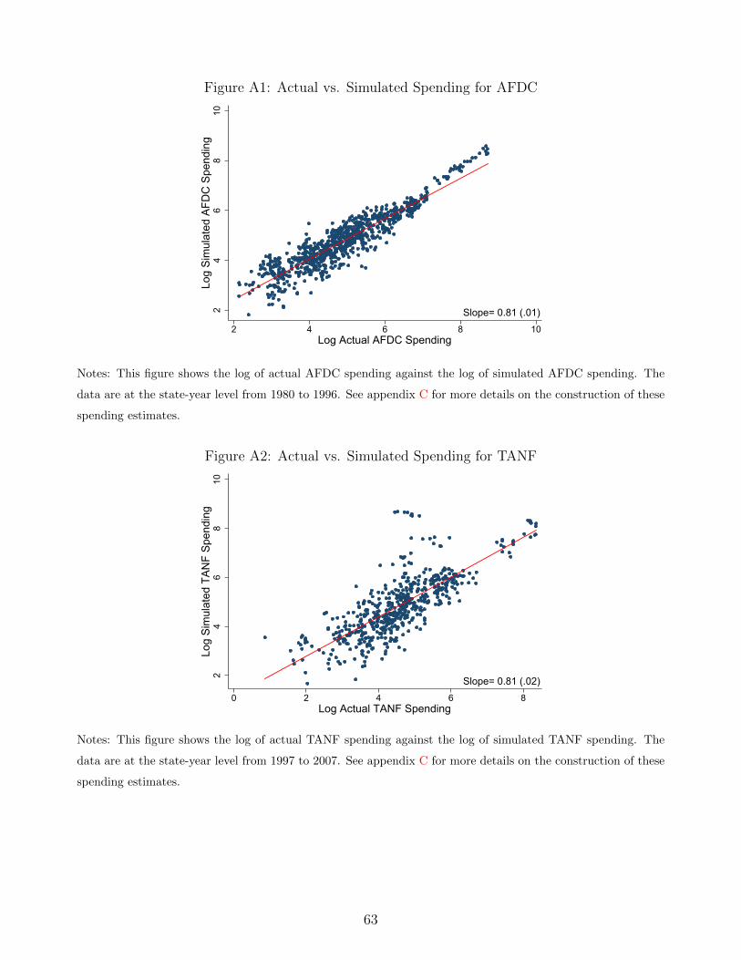
Figure A1: Actual vs. Simulated Spending for AFDC

24

68

10Lo

g Si

mul

ated

AFD

C S

pend

ing

2 4 6 8 10Log Actual AFDC Spending

Slope= 0.81 (.01)

Notes: This figure shows the log of actual AFDC spending against the log of simulated AFDC spending. The

data are at the state-year level from 1980 to 1996. See appendix C for more details on the construction of these

spending estimates.

Figure A2: Actual vs. Simulated Spending for TANF

24

68

10Lo

g Si

mul

ated

TAN

F Sp

endi

ng

0 2 4 6 8Log Actual TANF Spending

Slope= 0.81 (.02)

Notes: This figure shows the log of actual TANF spending against the log of simulated TANF spending. The


spending estimates.

63

Figure A3: Actual vs. Simulated Spending for SSI

02

46

8Lo

g Si

mul

ated

SSI

Spe

ndin

g

0 2 4 6 8Log Actual SSI Spending

Slope= .7 (.02)

Notes: This figure shows the log of actual SSI spending against the log of simulated SSI spending. The data are

at the state-year level from 1980 to 2007. See appendix C for more details on the construction of these spending

estimates.

Figure A4: Actual vs. Simulated Spending for SNAP

24

68

10Lo

g Si

mul

ated

SN

AP S

pend

ing

2 4 6 8Log Actual SNAP Spending

Slope= .91 (.01)

Notes: This figure shows the log of actual SNAP spending against the log of simulated SNAP spending. The


spending estimates.

64

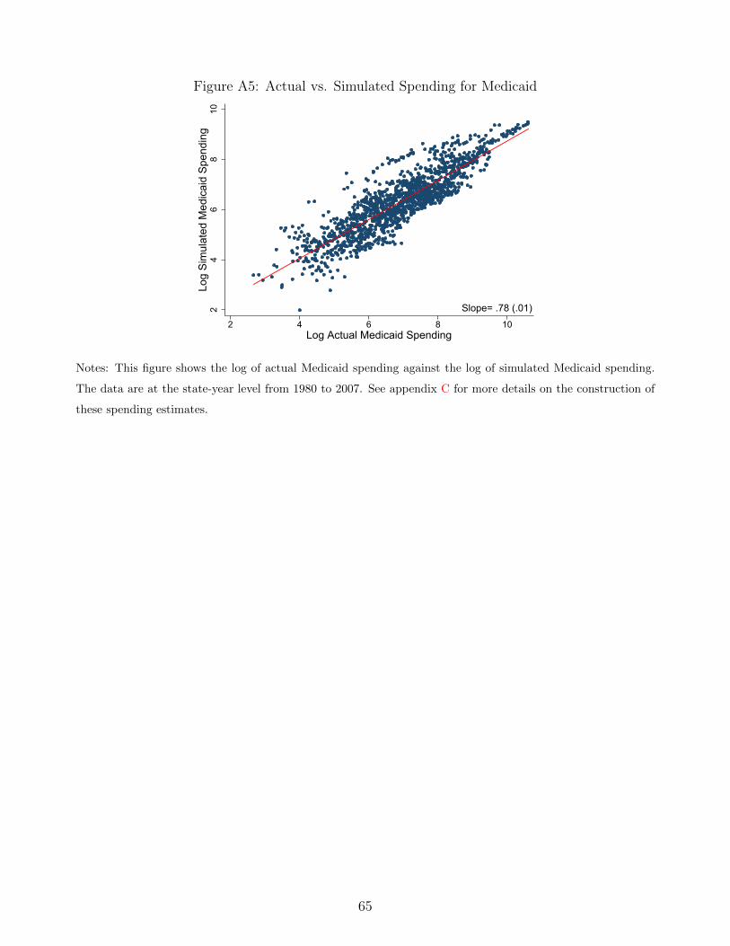
Figure A5: Actual vs. Simulated Spending for Medicaid

24

68

10Lo

g Si

mul

ated

Med

icai

d Sp

endi

ng

2 4 6 8 10Log Actual Medicaid Spending

Slope= .78 (.01)

Notes: This figure shows the log of actual Medicaid spending against the log of simulated Medicaid spending.

The data are at the state-year level from 1980 to 2007. See appendix C for more details on the construction of

these spending estimates.

65

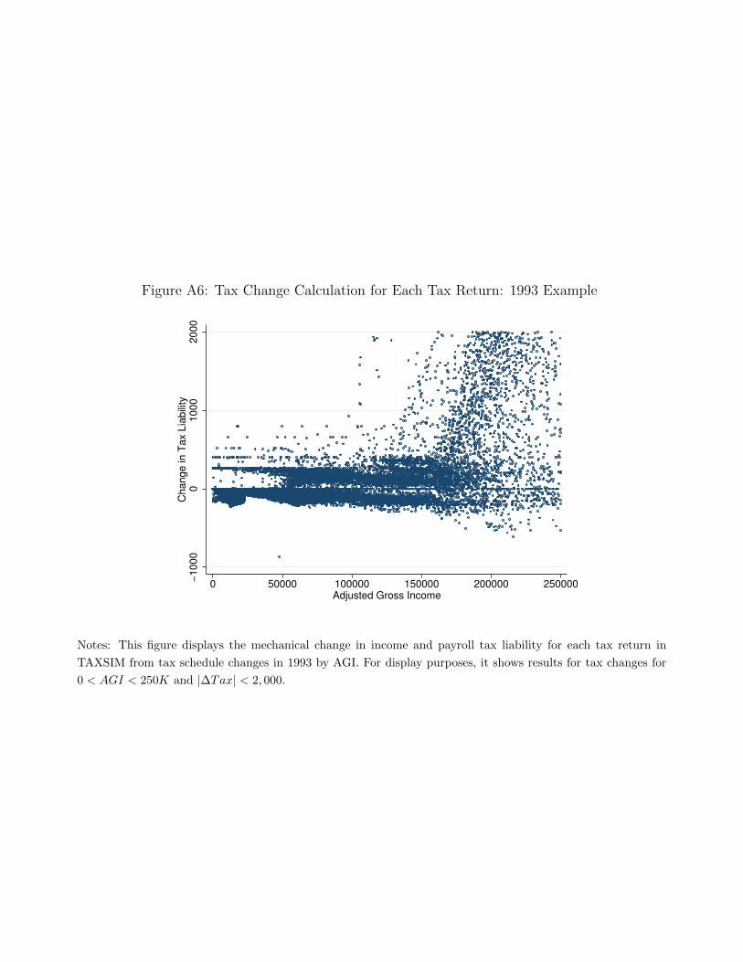
Figure A6: Tax Change Calculation for Each Tax Return: 1993 Example

−1000

01000

2000

Change in T

ax L

iabili

ty

0 50000 100000 150000 200000 250000Adjusted Gross Income

Notes: This figure displays the mechanical change in income and payroll tax liability for each tax return in

TAXSIM from tax schedule changes in 1993 by AGI. For display purposes, it shows results for tax changes for

0 < AGI < 250K and |∆Tax| < 2, 000.

Figure A7: Comparison of Aggregate Tax Changes with Romer & Romer Changes

−1

.5−

1−

.50

.51

Ta

x C

ha

ng

e a

s a

Sh

are

of

GD

P

1940 1960 1980 2000 2020Year

Romer Tax Measure Income and Payroll Tax Changes

Notes: This figure shows two postwar time series of tax changes: (1) the sum of all income and payroll tax

changes that Romer and Romer (2010) classify as exogenous and (2) the exogenous tax change measures of

Romer and Romer (2010). Both series are as a share of GDP. Some of the Romer and Romer (2010) tax changes

affect corporate taxes and other revenue sources, but the two series track each other fairly closely.

67

Figure A8: Favero and Giavazzi Orthogonality Test for Both Tax Change Series

A. Tax Changes for Top 10%

−.6

−.4

−.2

0.2

.4T

ax C

hange a

s a

Share

of G

DP

1940 1960 1980 2000 2020Year

Top 10% Tax Shock Orthogonalized Top 10% Tax Shock

B. Tax Changes for Bottom 90%

−.4

−.2

0.2

.4T

ax C

hange a

s a

Share

of G

DP

1940 1960 1980 2000 2020Year

Bot. 90% Tax Shock Orthogonalized Bot. 90% Tax Shock

Notes: This figure plots the raw time series of federal income and payroll tax changes as a share of GDP as well

as an orthogonalized time series of the residual of the tax change measure after partialling out lagged macro

aggregates, which are annual log changes in employment, inflation, government transfers as a share of GDP, and

federal debt as a share of GDP. The graphs show that the orthogonalized version is quite similar to the raw time

series, suggesting that these federal tax shock series for the top 10% and bottom 90% both pass the Favero and

Giavazzi (2012) orthogonality test. See data section for sources and section 3.4 for additional discussion.

68

Figure A9: Frisch Waugh Regression: Tax Changes for Top versus Bottom

1950

195119521953

1954

195519561957195819591960

1961 1962

1963

1964

1965

19661967196819691970

1971

1972 197319741975

1976

1977 1978

1979

19801981

1982

1983

19841985

1986

1987

1988

19891990

1991

1992

1993

1994

19951996199719981999

2000

2001

2002

2003

20042005 200620072008200920102011

−.6

−.4

−.2

0.2

.4C

ha

ng

e in

Ta

x L

iab

ility

fo

r T

op

10

% a

s %

of

GD

P

−.4 −.2 0 .2 .4Change in Tax Liability for Bottom 90% as % of GDP

Notes: This figure plots exogenous tax changes for those with AGI in top 10% by those for the bottom 90%.

Both tax changes are as a share of output. The figure also plots the predicted value of exogenous tax changes

for those in the top 10% from a simple bivariate regression on exogenous tax changes for those with AGI in the

bottom 90%. Years that fall below the best fit line had tax changes that went disproportionately to the top 10%

(given the magnitude of tax changes for the bottom 90% as a share of output).

69

Figure A10: Cumulative Growth in Emp-to-Pop Ratio and Employment: Lagged Tax Changes as Controls

A. Employment/Population B. Employment

-.1-.0

50

.05

Perc

enta

ge p

oint

s


Bottom 90 Top 10

-.1-.0

50

.05

Perc

ent


Bottom 90 Top 10

Notes: This figure shows event studies of a 1% of GDP tax increase on the state employment-to-population ratio and employment for those with AGI inthe bottom 90% nationally in blue and for those with AGI in the top 10% nationally in red. Specifically, the figure plots the estimates from the baselinespecification of equation 2 for the impact of tax changes in year h for the bottom 90%, αB90


controls for mechanical changes in AFDC, TANF, SNAP, SSI, and Medicaid spending as a percentage of state GDP, as well as cyclicality-quintile year fixedeffects. See section 2 for details. One and two year lags of tax changes and spending controls are also included. Standard errors are robust and clusteredby state; 95% confidence intervals are shown as dotted lines. The sample period is 1980-2007.

70

Figure A11: Cumulative Growth in Prices, GDP, and Earnings: Lagged Tax Changes as Controls

-.15

-.1-.0

50

.05

Perc

ent


A. Nominal GDP

-.2-.1

0.1

Perc

ent


B. ACCRA Index

-.2-.1

0.1

.2Pe

rcen

t


C. Real GDP (ACCRA)

-.10

.1.2

Perc

ent


D. Real GDP (Moretti HPI)-.1

5-.1

-.05

0.0

5Pe

rcen

t


E. Net Earnings

-.15

-.1-.0

50

.05

.1Pe

rcen

t


F. Consumption

-.2-.1

0.1

Perc

ent


G. Real Net Earnings (ACCRA)

-.15

-.1-.0

50

.05

.1Pe

rcen

t


H. Real Net Earnings (Moretti HPI)

Bottom 90 Top 10

Notes: This figure shows event studies of a 1% of GDP tax increase on outcomes for those with AGI in the bottom 90% nationally in blue and for thosewith AGI in the top 10% nationally in red. The outcomes are (a) nominal state GDP, (b) the ACCRA state price index PACCRA

s,t , (c) real state GDP using

PACCRAs,t , (d) real state GDP using PMoretti

s,t , (e) nominal net earnings, (f) consumption, (g) real net earnings using PACCRAs,t , and (h) real net earnings

using PMorettis,t . Specifically, the figure plots the estimates from the baseline specification of equation 2 for the impact of tax changes in year h for the

bottom 90%, αB90h , and the top 10%, αT10

h . The baseline specification includes controls for mechanical changes in AFDC, TANF, SNAP, SSI, and Medicaidspending as a percentage of state GDP, as well as cyclicality-quintile year fixed effects. See section 2 for details. One and two year lags of tax changes andspending controls are also included. Standard errors are robust and clustered by state; 95% confidence intervals are shown as dotted lines. The sampleperiod is 1980-2007 for (a)-(e) and (g)-(h). However, state consumption is only available since 1997, so the sample period for (f) is 1997-2007.

71

Figure A12: Cumulative Growth in State-level Labor Market Outcomes: Lagged Tax Changes as Controls

-.15

-.1-.0

50

.05

.1Pe

rcen

t


A. Payroll

-.1-.0

50

.05

Perc

enta

ge p

oint

s


B. Labor Force Participation Rate

-.06

-.04

-.02

0.0

2.0

4Pe

rcen

t


C. Hours

-.10

.1.2

.3Pe

rcen

t


D. Real Wage (ACCRA)-.1

-.05

0.0

5.1

.15

Perc

ent


E. Real Payroll (ACCRA)

-.04

-.02

0.0

2.0

4Pe

rcen

tage

poi

nts


F. Employment Rate

-.1-.0

50

.05

.1.1

5Pe

rcen

t


G. Wage

-.2-.1

0.1

.2.3

Perc

ent


H. Real Comp-Constant Wage (ACCRA)

Bottom 90 Top 10

Notes: This figure shows event studies of a 1% of GDP tax increase on outcomes for those with AGI in the bottom 90% nationally in blue and for thosewith AGI in the top 10% nationally in red. These outcomes are (a) nominal state payroll, (b) labor force participation rate, (c) mean hours worked amongthose who worked at least 48 weeks in the past year, (d) mean real wages using PACCRA

s,t , (e) real state payroll using PACCRAs,t , (f) employment rate, (g)

mean wages, and (h) real composition-constant average wages using PACCRAs,t . Specifically, the figure plots the estimates from the baseline specification

of equation 2 for the impact of tax changes in year h for the bottom 90%, αB90h , and the top 10%, αT10

h . The baseline specification includes controls formechanical changes in AFDC, TANF, SNAP, SSI, and Medicaid spending as a percentage of state GDP, as well as cyclicality-quintile year fixed effects. Seesection 2 for details. One and two year lags of tax changes and spending controls are also included. Standard errors are robust and clustered by state; 95%confidence intervals are shown as dotted lines. The sample period is 1980-2007.

72

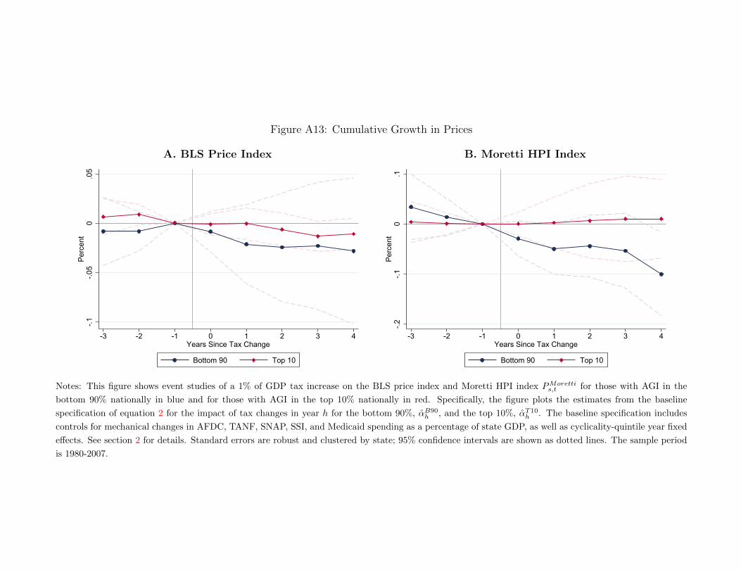
Figure A13: Cumulative Growth in Prices

A. BLS Price Index B. Moretti HPI Index

-.1-.0

50

.05

Perc

ent


Bottom 90 Top 10

-.2-.1

0.1

Perc

ent


Bottom 90 Top 10

Notes: This figure shows event studies of a 1% of GDP tax increase on the BLS price index and Moretti HPI index PMorettis,t for those with AGI in the

bottom 90% nationally in blue and for those with AGI in the top 10% nationally in red. Specifically, the figure plots the estimates from the baseline

specification of equation 2 for the impact of tax changes in year h for the bottom 90%, αB90h , and the top 10%, αT10

h . The baseline specification includes

controls for mechanical changes in AFDC, TANF, SNAP, SSI, and Medicaid spending as a percentage of state GDP, as well as cyclicality-quintile year fixed

effects. See section 2 for details. Standard errors are robust and clustered by state; 95% confidence intervals are shown as dotted lines. The sample period

is 1980-2007.

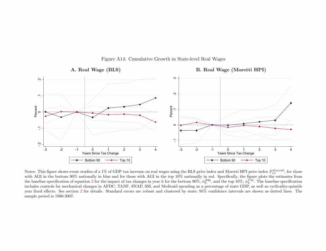
Figure A14: Cumulative Growth in State-level Real Wages

A. Real Wage (BLS) B. Real Wage (Moretti HPI)

-.2-.1

0.1

.2Pe

rcen

t


Bottom 90 Top 10

-.10

.1.2

.3Pe

rcen

t


Bottom 90 Top 10

Notes: This figure shows event studies of a 1% of GDP tax increase on real wages using the BLS price index and Moretti HPI price index PMorettis,t , for those

with AGI in the bottom 90% nationally in blue and for those with AGI in the top 10% nationally in red. Specifically, the figure plots the estimates fromthe baseline specification of equation 2 for the impact of tax changes in year h for the bottom 90%, αB90

h , and the top 10%, αT10h . The baseline specification

includes controls for mechanical changes in AFDC, TANF, SNAP, SSI, and Medicaid spending as a percentage of state GDP, as well as cyclicality-quintileyear fixed effects. See section 2 for details. Standard errors are robust and clustered by state; 95% confidence intervals are shown as dotted lines. Thesample period is 1980-2007.

Figure A15: Cumulative Growth in Employment-to-Population Ratio by Demographic Split

-.1-.0

50

.05

Perc

enta

ge p

oint

s


A. Skilled

-.1-.0

50

.05

.1Pe

rcen

tage

poi

nts


B. Unskilled

-.05

0.0

5.1

Perc

enta

ge p

oint

s


C. Aged 25-45

-.15

-.1-.0

50

.05

.1Pe

rcen

tage

poi

nts


D. Aged 45-60-.1

-.05

0.0

5Pe

rcen

tage

poi

nts


E. Men

-.1-.0

50

.05

Perc

enta

ge p

oint

s


F. Women

-.1-.0

50

.05

Perc

enta

ge p

oint

s


G. White

-.2-.1

5-.1

-.05

0.0

5Pe

rcen

tage

poi

nts


H. Non-White

Bottom 90 Top 10

Notes: This figure shows event studies of a 1% of GDP tax increase on the state employment-to-population ratio by demographic splits for those with AGIin the bottom 90% nationally in blue and for those with AGI in the top 10% nationally in red. Specifically, the figure plots the estimates from the baselinespecification of equation 2 for the impact of tax changes in year h for the bottom 90%, αB90


controls for mechanical changes in AFDC, TANF, SNAP, SSI, and Medicaid spending as a percentage of state GDP, as well as cyclicality-quintile year fixedeffects. See section 2 for details. See section A.2.2 for details on each demographic split. Standard errors are robust and clustered by state; 95% confidenceintervals are shown as dotted lines. The sample period is 1980-2007.

75

Figure A16: Cumulative Growth in Employment Rate by Demographic Split

-.04

-.02

0.0

2.0

4Pe

rcen

t


A. Skilled

-.1-.0

50

.05

.1Pe

rcen

t


B. Unskilled

-.06

-.04

-.02

0.0

2.0

4Pe

rcen

t


C. Aged 25-45

-.05

0.0

5Pe

rcen

t


D. Aged 45-60-.0

50

.05

Perc

ent


E. Men

-.06

-.04

-.02

0.0

2.0

4Pe

rcen

t


F. Women

-.04

-.02

0.0

2.0

4Pe

rcen

t


G. White

-.2-.1

0.1

.2Pe

rcen

t


H. Non-White

Bottom 90 Top 10

Notes: This figure shows event studies of a 1% of GDP tax increase on the state employment rate by demographic splits for those with AGI in the bottom90% nationally in blue and for those with AGI in the top 10% nationally in red. Specifically, the figure plots the estimates from the baseline specificationof equation 2 for the impact of tax changes in year h for the bottom 90%, αB90

h , and the top 10%, αT10h . The baseline specification includes controls for

mechanical changes in AFDC, TANF, SNAP, SSI, and Medicaid spending as a percentage of state GDP, as well as cyclicality-quintile year fixed effects. Seesection 2 for details. See section A.2.2 for details on each demographic split. Standard errors are robust and clustered by state; 95% confidence intervalsare shown as dotted lines. The sample period is 1980-2007.

76

Figure A17: Cumulative Growth in Labor Force Participation Rate by Demographic Split

-.1-.0

50

.05

Perc

enta

ge p

oint

s


A. Skilled

-.1-.0

50

.05

.1Pe

rcen

tage

poi

nts


B. Unskilled

-.04

-.02

0.0

2.0

4.0

6Pe

rcen

tage

poi

nts


C. Aged 25-45

-.15

-.1-.0

50

.05

.1Pe

rcen

tage

poi

nts


D. Aged 45-60-.1

-.05

0.0

5Pe

rcen

tage

poi

nts


E. Men

-.1-.0

50

.05

Perc

enta

ge p

oint

s


F. Women

-.1-.0

50

.05

Perc

enta

ge p

oint

s


G. White

-.3-.2

-.10

.1Pe

rcen

tage

poi

nts


H. Non-White

Bottom 90 Top 10

Notes: This figure shows event studies of a 1% of GDP tax increase on the state labor force participation rate by demographic splits for those with AGI inthe bottom 90% nationally in blue and for those with AGI in the top 10% nationally in red. Specifically, the figure plots the estimates from the baselinespecification of equation 2 for the impact of tax changes in year h for the bottom 90%, αB90


controls for mechanical changes in AFDC, TANF, SNAP, SSI, and Medicaid spending as a percentage of state GDP, as well as cyclicality-quintile year fixedeffects. See section 2 for details. See section A.2.2 for details on each demographic split. Standard errors are robust and clustered by state; 95% confidenceintervals are shown as dotted lines. The sample period is 1980-2007.

77

Figure A18: Cumulative Growth in Hours by Demographic Split

-.04

-.02

0.0

2.0

4.0

6Pe

rcen

t


A. Skilled

-.06

-.04

-.02

0.0

2.0

4Pe

rcen

t


B. Unskilled

-.04

-.02

0.0

2.0

4Pe

rcen

t


C. Aged 25-45

-.1-.0

50

.05

Perc

ent


D. Aged 45-60-.0

6-.0

4-.0

20

.02

.04

Perc

ent


E. Men

-.04

-.02

0.0

2.0

4.0

6Pe

rcen

t


F. Women

-.04

-.02

0.0

2.0

4Pe

rcen

t


G. White

-.1-.0

50

.05

.1Pe

rcen

t


H. Non-White

Bottom 90 Top 10

Notes: This figure shows event studies of a 1% of GDP tax increase on hours worked (if at least 48 weeks were worked in the past year) by demographicsplits for those with AGI in the bottom 90% nationally in blue and for those with AGI in the top 10% nationally in red. Specifically, the figure plots theestimates from the baseline specification of equation 2 for the impact of tax changes in year h for the bottom 90%, αB90

h , and the top 10%, αT10h . The

baseline specification includes controls for mechanical changes in AFDC, TANF, SNAP, SSI, and Medicaid spending as a percentage of state GDP, as wellas cyclicality-quintile year fixed effects. See section 2 for details. See section A.2.2 for details on each demographic split. Standard errors are robust andclustered by state; 95% confidence intervals are shown as dotted lines. The sample period is 1980-2007.

78

Figure A19: Cumulative Growth in Wage by Demographic Split

-.2-.1

0.1

.2Pe

rcen

t


A. Skilled

-.15

-.1-.0

50

.05

.1Pe

rcen

t


B. Unskilled

-.15

-.1-.0

50

.05

.1Pe

rcen

t


C. Aged 25-45

-.2-.1

0.1

.2Pe

rcen

t


D. Aged 45-60-.2

-.10

.1.2

Perc

ent


E. Men

-.2-.1

5-.1

-.05

0.0

5Pe

rcen

t


F. Women

-.15

-.1-.0

50

.05

.1Pe

rcen

t


G. White

-.20

.2.4

Perc

ent


H. Non-White

Bottom 90 Top 10

Notes: This figure shows event studies of a 1% of GDP tax increase on wages by demographic splits for those with AGI in the bottom 90% nationally inblue and for those with AGI in the top 10% nationally in red. Specifically, the figure plots the estimates from the baseline specification of equation 2 for theimpact of tax changes in year h for the bottom 90%, αB90

h , and the top 10%, αT10h . The baseline specification includes controls for mechanical changes in

AFDC, TANF, SNAP, SSI, and Medicaid spending as a percentage of state GDP, as well as cyclicality-quintile year fixed effects. See section 2 for details.See section A.2.2 for details on each demographic split. Standard errors are robust and clustered by state; 95% confidence intervals are shown as dottedlines. The sample period is 1980-2007.

79

Figure A20: Cumulative Growth in Real Wage by Demographic Split

-.2-.1

0.1

.2.3

Perc

ent


A. Skilled

-.2-.1

0.1

.2Pe

rcen

t


B. Unskilled

-.2-.1

0.1

.2Pe

rcen

t


C. Aged 25-45

-.4-.2

0.2

.4Pe

rcen

t


D. Aged 45-60-.2

-.10

.1.2

.3Pe

rcen

t


E. Men

-.2-.1

0.1

.2Pe

rcen

t


F. Women

-.2-.1

0.1

.2Pe

rcen

t


G. White

-.20

.2.4

.6Pe

rcen

t


H. Non-White

Bottom 90 Top 10

Notes: This figure shows event studies of a 1% of GDP tax increase on real wages using PACCRAs,t by demographic splits for those with AGI in the bottom

90% nationally in blue and for those with AGI in the top 10% nationally in red. Specifically, the figure plots the estimates from the baseline specificationof equation 2 for the impact of tax changes in year h for the bottom 90%, αB90

h , and the top 10%, αT10h . The baseline specification includes controls for

mechanical changes in AFDC, TANF, SNAP, SSI, and Medicaid spending as a percentage of state GDP, as well as cyclicality-quintile year fixed effects. Seesection 2 for details. See section A.2.2 for details on each demographic split. Standard errors are robust and clustered by state; 95% confidence intervalsare shown as dotted lines. The sample period is 1980-2007.

80

Figure A21: Cumulative Growth in Income by Type of Income

A. Total Income B. Dividends Income

-.15

-.1-.0

50

.05

Perc

ent


Bottom 90 Top 10

-2-1

01

2Pe

rcen

t


Bottom 90 Top 10

C. Rent Income D. Interest Income

-3-2

-10

12

Perc

ent


Bottom 90 Top 10

-.6-.4

-.20

.2.4

Perc

ent


Bottom 90 Top 10

Notes: This figure shows event studies of a 1% of GDP tax increase on outcomes for those with AGI in the bottom 90% nationally in blue and for those withAGI in the top 10% nationally in red. These outcomes are (a) total income, (b) dividends income, (c) rent income, and (d) interest income. Specifically, thefigure plots the estimates from the baseline specification of equation 2 for the impact of tax changes in year h for the bottom 90%, αB90

h , and the top 10%,αT10h . The baseline specification includes controls for mechanical changes in AFDC, TANF, SNAP, SSI, and Medicaid spending as a percentage of state

GDP, as well as cyclicality-quintile year fixed effects. See section 2 for details. Standard errors are robust and clustered by state; 95% confidence intervalsare shown as dotted lines. The sample period is 1980-2007.

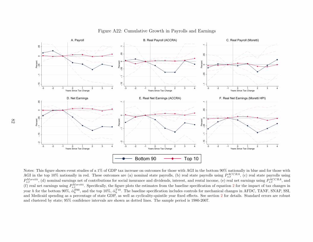
Figure A22: Cumulative Growth in Payrolls and Earnings

-.15

-.1-.0

50

.05

Perc

ent


A. Payroll

-.15

-.1-.0

50

.05

.1Pe

rcen

t


B. Real Payroll (ACCRA)

-.1-.0

50

.05

.1Pe

rcen

t


C. Real Payroll (Moretti)-.2

-.15

-.1-.0

50

.05

Perc

ent


D. Net Earnings

-.2-.1

0.1

Perc

ent


E. Real Net Earnings (ACCRA)

-.15

-.1-.0

50

.05

.1Pe

rcen

t


F. Real Net Earnings (Moretti HPI)

Bottom 90 Top 10

Notes: This figure shows event studies of a 1% of GDP tax increase on outcomes for those with AGI in the bottom 90% nationally in blue and for those withAGI in the top 10% nationally in red. These outcomes are (a) nominal state payrolls, (b) real state payrolls using PACCRA

s,t , (c) real state payrolls using

PMorettis,t , (d) nominal earnings net of contributions for social insurance and dividends, interest, and rental income, (e) real net earnings using PACCRA

s,t , and

(f) real net earnings using PMorettis,t . Specifically, the figure plots the estimates from the baseline specification of equation 2 for the impact of tax changes in

year h for the bottom 90%, αB90h , and the top 10%, αT10

h . The baseline specification includes controls for mechanical changes in AFDC, TANF, SNAP, SSI,and Medicaid spending as a percentage of state GDP, as well as cyclicality-quintile year fixed effects. See section 2 for details. Standard errors are robustand clustered by state; 95% confidence intervals are shown as dotted lines. The sample period is 1980-2007.

82

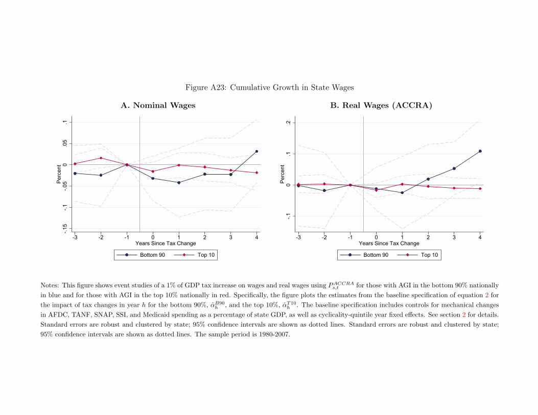
Figure A23: Cumulative Growth in State Wages

A. Nominal Wages B. Real Wages (ACCRA)

-.15

-.1-.0

50

.05

.1Pe

rcen

t


Bottom 90 Top 10

-.10

.1.2

Perc

ent


Bottom 90 Top 10

Notes: This figure shows event studies of a 1% of GDP tax increase on wages and real wages using PACCRAs,t for those with AGI in the bottom 90% nationally

in blue and for those with AGI in the top 10% nationally in red. Specifically, the figure plots the estimates from the baseline specification of equation 2 for

the impact of tax changes in year h for the bottom 90%, αB90h , and the top 10%, αT10

h . The baseline specification includes controls for mechanical changes

in AFDC, TANF, SNAP, SSI, and Medicaid spending as a percentage of state GDP, as well as cyclicality-quintile year fixed effects. See section 2 for details.

Standard errors are robust and clustered by state; 95% confidence intervals are shown as dotted lines. Standard errors are robust and clustered by state;

95% confidence intervals are shown as dotted lines. The sample period is 1980-2007.

Figure A24: Cumulative Growth in Part-time Employment Rate

-.04

-.02

0.0

2.0

4Pe

rcen

tage

poi

nts


Bottom 90 Top 10

Notes: This figure shows event studies of a 1% of GDP tax increase on the part-time employment rate for those with AGI in the bottom 90% nationally in

blue and for those with AGI in the top 10% nationally in red. Specifically, the figure plots the estimates from the baseline specification of equation 2 for the

impact of tax changes in year h for the bottom 90%, αB90h , and the top 10%, αT10

h . The baseline specification includes controls for mechanical changes in

AFDC, TANF, SNAP, SSI, and Medicaid spending as a percentage of state GDP, as well as cyclicality-quintile year fixed effects. See section 2 for details.

Standard errors are robust and clustered by state; 95% confidence intervals are shown as dotted lines. The sample period is 1980-2007.

Figure A25: Cumulative Growth in State Emp-to-Pop Ratio and Employment: Includes Non-Personal Income Taxes in Top Decile

A. Employment/Population B. Employment

-.1-.0

50

.05

Perc

enta

ge p

oint

s


Bottom 90 Top 10

-.1-.0

50

.05

.1Pe

rcen

t


Bottom 90 Top 10

Notes: This figure shows event studies of a 1% of GDP tax increase on the state employment-to-population ratio and employment for those with AGI in thebottom 90% nationally in blue and for those with AGI in the top 10% nationally in red. Specifically, the figure plots the estimates from the specification ofequation 2 for the impact of tax changes in year h for the bottom 90%, αB90

h , and the top 10%, αT10h . However, unlike the baseline specification definition for

tax changes for the top 10%, I also allocate the non-personal income tax changes to top earners in the same proportion as the top 10% shares are allocated.This is done in an attempt to resolve potential issues with exclusions of non-personal income taxes (corporate taxes, etc.) biasing estimates for the Top 10%group. The baseline specification includes controls for mechanical changes in AFDC, TANF, SNAP, SSI, and Medicaid spending as a percentage of stateGDP, as well as cyclicality-quintile year fixed effects. See section 2 for details. Standard errors are robust and clustered by state; 95% confidence intervalsare shown as dotted lines. The sample period is 1980-2007.

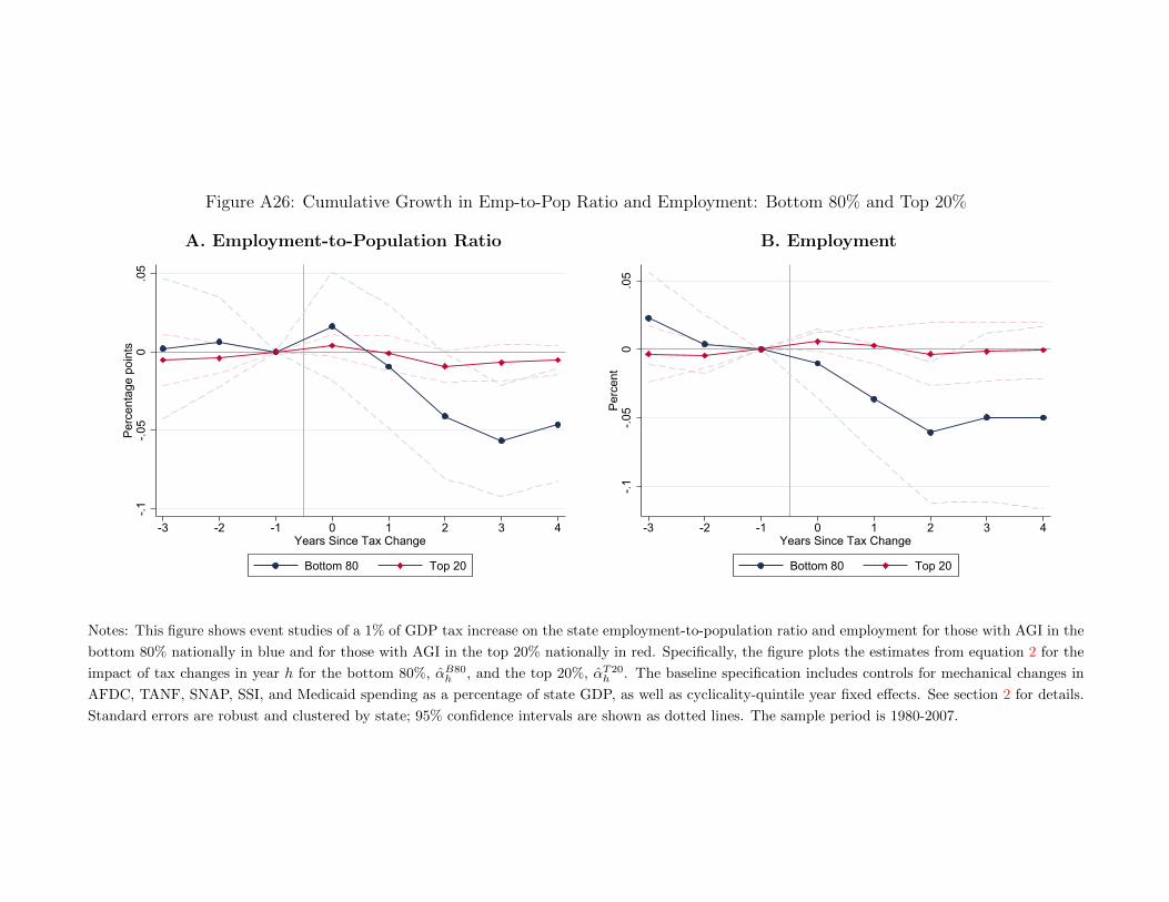
Figure A26: Cumulative Growth in Emp-to-Pop Ratio and Employment: Bottom 80% and Top 20%

A. Employment-to-Population Ratio B. Employment

-.1-.0

50

.05

Perc

enta

ge p

oint

s


Bottom 80 Top 20

-.1-.0

50

.05

Perc

ent


Bottom 80 Top 20

Notes: This figure shows event studies of a 1% of GDP tax increase on the state employment-to-population ratio and employment for those with AGI in the

bottom 80% nationally in blue and for those with AGI in the top 20% nationally in red. Specifically, the figure plots the estimates from equation 2 for the

impact of tax changes in year h for the bottom 80%, αB80h , and the top 20%, αT20

h . The baseline specification includes controls for mechanical changes in

AFDC, TANF, SNAP, SSI, and Medicaid spending as a percentage of state GDP, as well as cyclicality-quintile year fixed effects. See section 2 for details.

Standard errors are robust and clustered by state; 95% confidence intervals are shown as dotted lines. The sample period is 1980-2007.

Table A3: Summary Statistics

Panel A: State Summary StatisticsVariable Mean Std. Dev. Min. Max NYear 1980 2007 1400Log Employment 15.151 0.879 12.04 16.64 1400Log State GDP 26.585 0.976 23.36 28.43 1400Employment Rate 93.520 2.111 81.23 97.94 1400Emp/Pop 60.145 4.175 39.72 73.45 1400LFP Rate 64.277 3.676 46.27 76.74 1400Part-Time Emp Rate 18.747 3.655 10.06 37.94 1400Log Payroll 25.763 0.989 22.61 27.53 1400Log Hours 7.657 0.017 7.58 7.72 1400Log Wages 3.071 0.137 2.49 3.46 1400Log Comp-Constant Wages 2.996 0.122 2.45 3.36 1400Employment Growth 1.388 1.632 -6.77 10.35 1350GDP Growth 2.758 2.933 -32.89 25.76 1350Real GDP Growth (ACCRA) 2.655 3.692 -59.01 27.77 1246Real GDP Growth (Moretti) 2.670 3.273 -29.48 22.26 1350TB90s,t -0.075 0.186 -1.08 0.46 1400T T10s,t -0.013 0.171 -1.27 1.57 1400

Panel B: National Summary StatisticsVariable Mean Std. Dev. Min. Max NYear 1950 2007 58GDP Growth 3.366 2.144 -1.93 7.75 57Investment Growth 3.855 8.326 -17.67 24.13 57Residential Investment Growth 2.141 11.791 -23.47 35.05 57Consumption Growth 3.507 1.653 -0.83 7.12 57Durable Consumption Growth 4.956 6.192 -8.68 19.33 57Non-Durable Consumption Growth 2.653 1.422 -2.46 5.41 57TB90t -0.038 0.139 -0.45 0.28 58T T10t -0.023 0.135 -0.49 0.31 58

87

Table A4: 2-Year Change - Demographic Robustness

Panel A: SkillSkilled LFP Rate Emp Rate Hours Wage Real WageBottom 90 -2.21* -0.56 0.24 -1.05 1.91

(1.20) (0.45) (0.93) (3.51) (4.53)Top 10 0.03 -0.33* 0.08 -0.87 -0.43

(0.40) (0.19) (0.32) (1.34) (0.96)UnskilledBottom 90 0.74 -2.12* -2.11*** 0.69 2.31

(1.21) (1.20) (0.79) (2.59) (3.01)Top 10 -0.53* 0.29 0.48*** -0.76 -0.36

(0.32) (0.28) (0.17) (0.96) (0.99)

Panel B: AgeAged 25-45 LFP Rate Emp Rate Hours Wage Real WageBottom 90 0.53 -2.52** -0.49 -2.85 -0.33

(0.98) (0.94) (0.63) (2.84) (3.66)Top 10 -0.17 0.08 0.20 -1.33 -0.91

(0.35) (0.28) (0.23) (1.06) (0.97)Aged 45-60Bottom 90 0.65 -2.17*** -2.31** -1.92 0.09

(1.48) (0.69) (0.87) (3.44) (4.69)Top 10 0.58 -0.03 0.17 -0.21 0.46

(0.46) (0.22) (0.33) (2.01) (1.62)

Panel C: SexMen LFP Rate Emp Rate Hours Wage Real WageBottom 90 -0.52 -1.95** -0.91 -2.38 0.26

(0.98) (0.83) (0.78) (2.92) (3.95)Top 10 -0.21 0.20 0.26 -0.23 0.15

(0.34) (0.27) (0.22) (1.45) (1.09)WomenBottom 90 -0.50 -1.44 -1.15 -2.13 -0.00

(0.94) (0.97) (0.92) (2.27) (2.80)Top 10 -0.30 -0.15 0.29 -1.71 -1.14

(0.39) (0.23) (0.32) (1.39) (1.49)

Panel D: RaceWhite LFP Rate Emp Rate Hours Wage Real WageBottom 90 0.03 -1.68** -1.00 -3.10 -0.73

(0.89) (0.75) (0.64) (2.57) (3.41)Top 10 -0.38 -0.02 0.20 -0.45 -0.11

(0.40) (0.22) (0.23) (1.62) (1.28)Non-WhiteBottom 90 -6.25** 0.01 -2.54 5.54 7.52

(3.08) (2.20) (1.78) (5.82) (7.10)Top 10 0.89 0.40 0.93 -3.16 -1.51

(1.05) (0.88) (0.69) (2.43) (3.01)

Notes: This table presents state-level estimates of two-year tax changes for different demographic groups. Each

specification is the same as column 1 in Table 1. The subsample (demographic group) of outcomes drawn from

the CPS varies, as specified in the first column. In the cases of the labor force participation rate and employment

rate, the outcomes are the simple difference, i.e., Ys,t − Ys,t−2, rather than the ratio described in equation 3.

Hours are restricted to those working at least 48 weeks in the past year. See section A.2.2 for details on each

demographic split. In each specification, I absorb state-specific effects and cluster standard errors by state (***

p<0.01, ** p<0.05, * p<0.1). The sample period is 1980-2007.

88

Table A5: 2-Year Change - Policy Robustness (Additional)(1) (2) (3) (4) (5) (6)

EmploymentBottom 90 -4.74** -3.21** -3.61** -4.74** -3.15** -3.43**

(1.79) (1.54) (1.50) (1.79) (1.49) (1.55)Top 10 0.16 -0.10 0.29 0.16 0.22 0.21

(0.93) (0.71) (0.83) (0.93) (0.88) (0.89)State GDPBottom 90 -12.12*** -11.65*** -12.28*** -12.11*** -11.08*** -11.98***

(2.19) (2.22) (2.22) (2.19) (1.99) (2.21)Top 10 0.40 0.39 0.87 0.40 0.75 0.75

(1.03) (0.91) (0.89) (1.03) (0.89) (0.97)Employment RateBottom 90 -1.98* -1.79** -1.76** -1.98* -1.62** -1.72**

(0.99) (0.82) (0.78) (0.99) (0.77) (0.79)Top 10 0.05 0.06 0.05 0.05 0.05 0.07

(0.22) (0.22) (0.21) (0.22) (0.21) (0.22)Emp/Pop

Bottom 90 -1.76 -1.66 -1.59 -1.76 -1.43 -1.52(1.19) (1.00) (0.95) (1.19) (0.94) (0.96)

Top 10 -0.26 -0.31 -0.22 -0.26 -0.24 -0.23(0.35) (0.34) (0.32) (0.35) (0.33) (0.34)

PayrollBottom 90 -8.78*** -8.36*** -8.72*** -8.80*** -7.49*** -8.36***

(2.95) (2.55) (2.54) (2.95) (2.38) (2.61)Top 10 0.09 -0.13 0.45 0.09 0.32 0.34

(1.10) (0.83) (0.90) (1.10) (0.95) (1.03)Net EarningsBottom 90 -11.58*** -10.34*** -10.86*** -11.57*** -9.88*** -10.56***

(2.11) (1.96) (1.99) (2.11) (1.77) (1.94)Top 10 0.59 0.57 0.83 0.59 0.72 0.75

(0.73) (0.79) (0.64) (0.73) (0.64) (0.72)

Controls1) COLA Y N N N N N2) SNAP Benefits x State N Y N N N N3) SNAP Benefits Per Household N N Y N N N4) FPL x State N N N Y N N5) FMAP N N N N Y N6) Max AFDC + TANF Benefits N N N N N Y

Notes: This table presents state-level estimates of two-year changes in taxes for different groups on economic

activity using a variety of ways to account for sensitivity to state-specific policies. Each specification is the same as

column 1 in Table 1 with additional controls. Column 1 controls for the annual cost of living adjustment (COLA).

Columns 2 and 3 control for the ratio of total Supplemental Nutrition Assistance Program (SNAP) benefits to

GDP, calculated in different ways. Column 4 controls for the Federal Poverty Level (FPL) interacted with state

dummies. Column 5 controls for the Federal Medical Assistance Percentage (FMAP). Column 6 controls for

total AFDC and TANF payments, as determined by the maximum payment for the modal households. See

sections A.2 and A.3 for more details on these controls. Standard errors are clustered by state (*** p<0.01, **

p<0.05, * p<0.1). The sample period is 1980-2007.

89

Table A6: State-level Effects of Tax Changes by Income Group on Economic Activity: Cyclical Robustness

(1) (2) (3) (4) (5) (6) (7) (8) (9) (10) (11) (12)Employment RateBottom 90 -1.74** -2.39*** -1.80** -1.89** -1.42** -2.33*** -2.44*** -2.26** -2.54** -1.70* -2.01** -1.95*

(0.79) (0.73) (0.73) (0.80) (0.56) (0.78) (0.83) (0.79) (0.81) (0.95) (0.72) (0.99)Top 10 0.05 0.14 0.14 -0.32 0.07 0.19 0.06 0.16 0.08 -0.01 -0.03 0.05

(0.21) (0.21) (0.22) (0.23) (0.18) (0.24) (0.22) (0.25) (0.21) (0.23) (0.28) (0.22)Emp/Pop

Bottom 90 -1.53 -1.62* -1.03 -1.08 -0.49 -1.59* -1.54 -1.64 -1.88 -1.39 -1.73 -1.78(0.96) (0.89) (0.99) (0.97) (0.89) (0.94) (0.94) (0.95) (1.05) (1.08) (1.45) (1.18)

Top 10 -0.24 -0.12 0.02 -0.45 -0.24 -0.06 -0.20 -0.05 -0.11 -0.26 -0.25 -0.27(0.33) (0.33) (0.39) (0.33) (0.31) (0.36) (0.34) (0.35) (0.36) (0.32) (0.38) (0.34)

PayrollBottom 90 -8.37*** -7.45** -4.93* -7.95*** -5.24* -7.09** -7.56** -6.18 -7.71* -8.17** -8.38* -8.79***

(2.61) (3.10) (2.55) (2.20) (2.80) (3.27) (2.91) (4.62) (3.74) (3.06) (3.80) (2.94)Top 10 0.32 0.47 -0.07 -0.25 0.11 0.34 -0.12 0.34 -0.05 -0.09 -0.12 0.08

(1.01) (0.83) (0.85) (0.81) (0.72) (0.85) (0.70) (0.84) (0.75) (1.03) (0.81) (1.11)Net EarningsBottom 90 -10.59*** -7.99** -5.10* -10.84*** -6.73** -7.79** -7.89** -6.28 -8.00* -10.15*** -9.94*** -11.47***

(1.95) (3.30) (2.56) (1.91) (2.75) (3.39) (3.25) (4.50) (3.86) (2.13) (2.21) (2.11)Top 10 0.73 0.89 0.19 -0.13 0.55 0.65 0.49 0.63 0.40 0.52 0.40 0.58

(0.70) (0.87) (0.85) (0.63) (0.83) (0.78) (0.79) (0.84) (0.80) (0.71) (0.44) (0.73)Controls1) Baseline Cyclicality Y N N N N N N N N Y Y Y2) Year N Y N N N Y Y Y Y N N N3) σGDPPC Cyclicality N N Y N N N N N N N N N4) Alternate β-diff Control #1 N N N Y N N N N N N N N5) Alternate β-diff Control #2 N N N N Y N N N N N N N6) Oil Price x State N N N N N Y N N N Y N N7) Real Interest Rate x State N N N N N N Y N N Y N N8) Oil Price x State + Region Y N N N N N N Y N N Y N9) Real Interest Rate x State + Region N N N N N N N N Y N Y N10) State Trends N N N N N N N N N N N Y

Notes: This table presents state-level estimates of two-year changes in taxes for different groups on economic activity using a variety of ways to accountfor state-specific cyclicality, trends, and sensitivity to other macro shocks. Each specification is the same as column 1 in Table 1 other than the controls.The first five columns present different ways to account for state-specific cyclicality (see section 2.1.1 or appendix B.1 for details); (1) baseline specificationwith cyclicality-quintile by year fixed effects, (2) year fixed effects, (3) cyclicality-quintile by year fixed effects where the quintiles are defined based on thestandard deviation in state GDP per capita, (4) cyclicality-decile by year fixed effects, and (5) cyclicality-quintile by year fixed effects that group statesonly using the years before the sample (i.e., before 1980). The next five columns show controls for state-specific sensitivity to other shocks and trends; (6)controls for oil price interacted with state dummies, (7) controls for real interest rate interacted with state dummies, (8) and (9) add region fixed effects to(6) and (7), and (10) includes state-specific trends. Standard errors are clustered by state (*** p<0.01, ** p<0.05, * p<0.1) in all specifications other than(8) and (9), which are clustered by region. The sample period is 1980-2007. See appendix A.2 for data definitions and sources.

90

Table A7: State-level Effects of Tax Changes by Income Group on Economic Activity: Policy Robustness

(1) (2) (3) (4) (5) (6) (7) (8) (9) (10) (11) (12)Employment RateBottom 90 -1.68** -1.77** -1.74** -1.74** -1.78** -1.74** -1.68** -1.75** -1.74** -1.78** -1.75** -1.78**

(0.80) (0.79) (0.79) (0.79) (0.78) (0.79) (0.81) (0.80) (0.79) (0.79) (0.80) (0.80)Top 10 0.06 0.04 0.04 0.04 0.05 0.05 0.05 0.05 0.05 0.04 0.05 0.06

(0.20) (0.21) (0.21) (0.21) (0.21) (0.21) (0.21) (0.22) (0.21) (0.21) (0.21) (0.21)Emp/Pop

Bottom 90 -1.35 -1.52 -1.53 -1.53 -1.59* -1.53 -1.48 -1.52 -1.53 -1.52 -1.53 -1.53(0.95) (0.97) (0.96) (0.96) (0.95) (0.96) (0.98) (0.96) (0.96) (0.98) (0.96) (0.98)

Top 10 -0.20 -0.24 -0.24 -0.26 -0.23 -0.24 -0.24 -0.25 -0.24 -0.24 -0.24 -0.23(0.30) (0.34) (0.33) (0.33) (0.33) (0.33) (0.33) (0.33) (0.33) (0.33) (0.33) (0.31)

PayrollBottom 90 -7.82*** -8.54*** -8.38*** -8.37*** -8.60*** -8.37*** -8.54*** -8.30*** -8.38*** -8.46*** -8.39*** -8.72***

(2.55) (2.62) (2.61) (2.61) (2.53) (2.60) (2.61) (2.63) (2.61) (2.61) (2.62) (2.58)Top 10 0.47 0.28 0.29 0.29 0.36 0.33 0.31 0.25 0.32 0.26 0.33 0.20

(0.88) (1.03) (1.01) (1.00) (0.98) (1.02) (1.03) (0.92) (1.01) (0.96) (1.01) (0.90)Net EarningsBottom 90 -10.21*** -10.72*** -10.59*** -10.59*** -10.65*** -10.59*** -10.55*** -10.53*** -10.59*** -10.65*** -10.59*** -10.57***

(1.95) (1.97) (1.95) (1.94) (1.92) (1.97) (1.97) (1.97) (1.96) (1.96) (1.96) (1.99)Top 10 0.83 0.69 0.75 0.69 0.74 0.73 0.73 0.67 0.73 0.69 0.73 0.67

(0.63) (0.69) (0.72) (0.68) (0.69) (0.70) (0.69) (0.67) (0.70) (0.68) (0.70) (0.65)Controls1) Government Transfers Per Capita Y N N N N N N N N N N N2) Federal IG Spending Per Capita N Y N N N N N N N N N N3) Minimum Wage N N Y N N N N N N N N Y4) OASDI N N N Y N N N N N N N Y5) Supplemental Security Income N N N N Y N N N N N N Y6) Max SNAP Benefits N N N N N Y N N N N N Y7) Medicaid Benefits N N N N N N Y N N N N Y8) AFDC + TANF Benefits N N N N N N N Y N N N Y9) Mechanical Change in AFDC & TANF N N N N N N N N Y N N Y10) Mechanical Change in SNAP & SSI N N N N N N N N N Y N Y11) Mechanical Change in Medicaid N N N N N N N N N N Y Y

Notes: This table presents state-level estimates of two-year changes in taxes for different groups on economic activity using a variety of ways to accountfor sensitivity to state-specific policies. Each specification is the same as column 1 in Table 1 with additional controls. Columns 1 and 2 control fortotal state transfers per capita and total federal transfers to a state per capita, respectively. Column 3 controls for the minimum wage. Columns 4-11control for the following as a share of state GDP: OASDI payments, Supplemental Security Income payments, SNAP benefits (assuming max allotment perrecipient), Medicaid vendor payments, AFDC and TANF payments, mechanical changes in AFDC and TANF spending, mechanical changes in SNAP andSSI spending, mechanical changes in Medicaid spending. See sections A.2, A.3, and C for more details on these controls and on the microsimulation-modelbased mechanical changes. Standard errors are clustered by state (*** p<0.01, ** p<0.05, * p<0.1). The sample period is 1980-2007.

91

Table A8: State-level Effects of Tax Changes by Income Group on State GDP: Cyclical Robustness(1) (2) (3) (4) (5) (6) (7) (8) (9) (10) (11) (12)

Panel A: Distributed Lag Model of Tax Changes for Different Income GroupsTB90s,t -2.05 -1.60 0.63 -1.76 -0.69 -1.91 -0.13 -1.25 -0.07 -1.06 -1.15 -1.65

(2.18) (2.44) (1.74) (2.33) (1.98) (2.75) (1.90) (3.81) (2.72) (2.36) (2.64) (2.48)TB90s,t−1 -7.39*** -8.15*** -5.24*** -6.69*** -6.71*** -7.95*** -7.54*** -7.51** -7.51*** -6.64*** -6.83*** -7.29***

(1.34) (1.95) (1.30) (1.15) (1.50) (2.11) (1.83) (2.82) (2.23) (1.32) (1.61) (1.32)TB90s,t−2 0.25 -1.09 -0.85 -0.25 0.71 -0.75 -0.97 -0.56 -0.98 0.65 0.53 0.55

(1.44) (1.71) (1.34) (1.55) (1.71) (1.80) (1.65) (2.39) (2.31) (1.72) (2.18) (1.77)T T10s,t 1.05* 0.96 0.55 0.53 1.02 0.90 0.66 0.85 0.74 0.95 0.90*** 0.84

(0.58) (0.60) (0.64) (0.63) (0.64) (0.61) (0.52) (0.60) (0.54) (0.61) (0.20) (0.65)T T10s,t−1 0.10 -0.08 -0.53 -0.11 0.03 -0.32 -0.59 -0.24 -0.48 -0.33 -0.25 -0.18

(0.70) (0.58) (0.67) (0.62) (0.57) (0.56) (0.61) (0.51) (0.53) (0.74) (0.52) (0.76)T T10s,t−2 -0.12 -0.08 -0.65 -0.44 0.09 -0.47 -0.51 -0.24 -0.46 -0.67 -0.59 -0.42

(0.57) (0.57) (0.57) (0.65) (0.56) (0.54) (0.53) (0.36) (0.42) (0.62) (0.36) (0.59)B90 Sum: βt + βt−1 + βt−2 -9.19*** -10.84** -5.45* -8.70** -6.69* -10.62* -8.64** -9.31 -8.55 -7.04* -7.45 -8.39*

(3.40) (5.09) (2.95) (3.44) (3.94) (5.69) (3.85) (7.66) (5.34) (3.91) (4.50) (4.27)T10 Sum: βt + βt−1 + βt−2 1.03 0.81 -0.64 -0.02 1.14 0.12 -0.44 0.37 -0.21 -0.05 0.06 0.24

(1.56) (1.44) (1.52) (1.48) (1.50) (1.36) (1.29) (1.13) (1.13) (1.68) (0.75) (1.71)Bottom - Top: -10.22** -11.65** -4.81 -8.69** -7.83* -10.73* -8.20* -9.68 -8.35 -6.99 -7.51 -8.63*

(3.96) (5.48) (3.50) (3.75) (4.45) (5.98) (4.42) (8.18) (6.02) (4.45) (4.88) (4.84)

Panel B: Two-Year ChangesBottom 90 -11.98*** -13.16*** -7.60*** -11.71*** -9.81*** -12.81*** -12.78*** -11.70* -12.36** -11.64*** -11.58*** -11.98***

(2.21) (4.17) (2.37) (2.21) (3.05) (4.46) (3.79) (5.89) (4.77) (2.28) (2.29) (2.20)Top 10 0.75 0.90 -0.10 0.18 0.74 0.53 0.26 0.65 0.32 0.24 0.31 0.38



Notes: This table presents analogous results to Table 2 for state GDP. The first five columns present different ways to account for state-specific cyclicality(see section 2.1.1 or appendix B.1 for details); (1) baseline specification with cyclicality-quintile by year fixed effects, (2) year fixed effects, (3) cyclicality-quintile by year fixed effects where the quintiles are defined based on the standard deviation in state GDP per capita, (4) cyclicality-decile by year fixedeffects, and (5) cyclicality-quintile by year fixed effects that group states only using the years before the sample (i.e., before 1980). The next five columnsshow controls for state-specific sensitivity to other shocks and trends; (6) controls for oil price interacted with state dummies, (7) controls for real interestrate interacted with state dummies, (8) and (9) add region fixed effects to (6) and (7), and (10) includes state-specific trends. Standard errors are clusteredby state (*** p<0.01, ** p<0.05, * p<0.1) in all specifications other than (8) and (9), which are clustered by region. The sample period is 1980-2007. Seeappendix A.2 for data definitions and sources.

92

Table A9: State-level Effects of Tax Changes by Income Group on State GDP: Policy Robustness(1) (2) (3) (4) (5) (6) (7) (8) (9) (10) (11) (12)

Panel A: Distributed Lag Model of Tax Changes for Different Income GroupsTB90s,t -2.06 -2.27 -2.07 -2.58 -1.41 -3.07 -2.11 -1.57 -2.10 -2.31 -2.03 -2.12

(2.11) (2.17) (2.18) (2.13) (1.81) (2.00) (2.08) (2.18) (2.20) (2.15) (2.19) (1.85)TB90s,t−1 -7.54*** -7.45*** -7.31*** -6.39*** -5.14*** -6.59*** -7.19*** -6.91*** -7.28*** -7.91*** -7.36*** -4.13***

(1.48) (1.36) (1.34) (1.33) (1.20) (1.30) (1.37) (1.26) (1.33) (1.41) (1.35) (1.34)TB90s,t−2 0.38 0.11 0.30 2.15 0.43 0.15 -0.16 0.54 0.19 0.30 0.28 1.12

(1.37) (1.44) (1.43) (1.48) (1.35) (1.44) (1.42) (1.42) (1.45) (1.40) (1.44) (1.24)T T10s,t 0.94 1.03* 1.04* 0.97* 0.98 1.39*** 0.86 1.00* 1.05* 1.02** 1.07* 0.77*

(0.57) (0.59) (0.58) (0.56) (0.68) (0.42) (0.58) (0.57) (0.58) (0.49) (0.58) (0.46)T T10s,t−1 0.15 0.06 0.11 0.12 0.30 0.18 0.07 0.16 0.09 0.08 0.08 0.26

(0.62) (0.70) (0.71) (0.65) (0.54) (0.52) (0.70) (0.64) (0.71) (0.66) (0.70) (0.40)T T10s,t−2 0.05 -0.16 -0.10 -0.15 0.17 -0.15 -0.17 -0.02 -0.13 -0.22 -0.13 0.24

(0.53) (0.57) (0.56) (0.54) (0.52) (0.43) (0.55) (0.53) (0.57) (0.53) (0.56) (0.34)B90 Sum: βt + βt−1 + βt−2 -9.22*** -9.60*** -9.09** -6.82* -6.13** -9.50*** -9.46*** -7.94** -9.18*** -9.92*** -9.11** -5.14**

(3.03) (3.43) (3.41) (3.48) (2.63) (3.18) (3.33) (3.32) (3.42) (3.31) (3.42) (2.50)T10 Sum: βt + βt−1 + βt−2 1.14 0.93 1.05 0.95 1.45 1.43 0.76 1.14 1.01 0.89 1.02 1.27

(1.35) (1.58) (1.56) (1.48) (1.56) (1.04) (1.55) (1.43) (1.56) (1.39) (1.56) (0.96)Bottom - Top: -10.36*** -10.54** -10.14** -7.77* -7.58** -10.93*** -10.22** -9.08** -10.20** -10.82*** -10.13** -6.41**

(3.46) (4.03) (3.97) (3.96) (3.09) (3.39) (3.93) (3.77) (3.97) (3.81) (3.97) (2.68)

Panel B: Two-Year ChangesBottom 90 -11.43*** -12.23*** -11.98*** -11.97*** -12.01*** -11.97*** -11.85*** -11.91*** -11.99*** -12.09*** -11.98*** -11.94***

(2.17) (2.23) (2.21) (2.18) (2.14) (2.22) (2.21) (2.23) (2.21) (2.19) (2.21) (2.16)Top 10 0.90 0.69 0.80 0.66 0.76 0.77 0.76 0.69 0.75 0.69 0.76 0.66



Notes: This table presents analogous results to Table 3 for state GDP. Columns 1 and 2 control for total state transfers per capita and total federal transfersto a state per capita, respectively. Column 3 controls for the minimum wage. Columns 4-11 control for the following as a share of state GDP: OASDIpayments, Supplemental Security Income payments, SNAP benefits (assuming max allotment per recipient), Medicaid vendor payments, AFDC and TANFpayments, mechanical changes in AFDC and TANF spending, mechanical changes in SNAP and SSI spending, mechanical changes in Medicaid spending.See sections A.2, A.3, and C for more details on these controls and on the microsimulation-model based mechanical changes. Standard errors are clusteredby state (*** p<0.01, ** p<0.05, * p<0.1). The sample period is 1980-2007.

93

Table A10: State-level Effects of Tax Changes by Income Group on Real State GDP: Cyclical Robustness(1) (2) (3) (4) (5) (6) (7) (8) (9) (10) (11) (12)

Panel A: Distributed Lag Model of Tax Changes for Different Income GroupsTB90s,t -0.29 0.02 3.44 -0.24 1.61 0.06 0.06 -0.12 0.24 0.17 -0.38 -1.46

(2.83) (2.52) (2.21) (3.54) (2.54) (2.84) (1.67) (4.03) (1.91) (3.37) (3.68) (3.39)TB90s,t−1 -8.40*** -10.85*** -7.74*** -6.80*** -8.35*** -10.71*** -10.86*** -10.65** -11.16** -8.19** -8.91** -9.11***

(2.85) (2.87) (1.95) (2.36) (2.74) (2.97) (3.37) (4.20) (4.20) (3.18) (3.81) (2.97)TB90s,t−2 2.11 0.08 -0.33 3.52 2.36 -0.10 -1.09 -0.24 -1.09 1.17 1.08 1.64

(2.11) (1.65) (1.99) (2.66) (2.09) (1.78) (2.69) (1.21) (1.45) (2.64) (2.40) (2.65)T T10s,t 0.91 1.49 0.58 1.49 1.33 1.48 1.02 1.36 1.12 0.62 0.67 0.68

(0.99) (1.12) (1.03) (0.97) (1.07) (1.17) (0.96) (1.15) (0.95) (1.04) (0.91) (0.96)T T10s,t−1 0.88 0.91 0.40 1.37* 0.79 0.81 0.18 0.71 0.35 0.32 0.50 0.63

(0.61) (0.78) (0.70) (0.71) (0.68) (0.79) (0.86) (0.77) (0.71) (0.69) (0.56) (0.61)T T10s,t−2 -0.12 -0.00 -0.37 -0.99 0.14 -0.21 -0.68 -0.19 -0.59 -0.85 -0.69 -0.42

(0.77) (0.81) (0.89) (1.06) (0.76) (0.84) (1.04) (0.75) (1.00) (0.84) (0.55) (0.79)B90 Sum: βt + βt−1 + βt−2 -6.59 -10.75** -4.62 -3.52 -4.39 -10.76** -11.89* -11.01 -12.01** -6.85 -8.21 -8.92

(4.97) (4.27) (3.88) (6.03) (4.85) (4.84) (6.01) (6.73) (5.05) (6.66) (7.58) (6.68)T10 Sum: βt + βt−1 + βt−2 1.67 2.40 0.61 1.87 2.27 2.09 0.52 1.88 0.89 0.09 0.47 0.89

(1.33) (1.83) (1.59) (1.51) (1.75) (1.87) (1.81) (1.72) (1.57) (1.45) (1.12) (1.26)Bottom - Top: -8.26 -13.14** -5.23 -5.39 -6.66 -12.85** -12.41** -12.90 -12.90** -6.94 -8.68 -9.81

(5.10) (5.17) (4.33) (6.19) (5.42) (5.69) (5.74) (7.42) (5.29) (6.67) (7.29) (6.79)

Panel B: Two-Year ChangesBottom 90 -9.70*** -13.18*** -6.96*** -8.98** -8.05** -13.27*** -14.28*** -12.54* -14.15** -10.22** -10.87** -11.32***

(3.46) (3.53) (2.36) (3.63) (3.39) (3.82) (3.78) (5.66) (4.55) (4.06) (4.51) (3.81)Top 10 1.44* 2.09 0.66 2.30** 1.57 1.83 1.03 1.86 1.17 0.49 0.88 1.08



Notes: This table presents analogous results to Table 2 for real state GDP using the ACCRA price index PACCRAs,t . The first five columns present different

ways to account for state-specific cyclicality (see section 2.1.1 or appendix B.1 for details); (1) baseline specification with cyclicality-quintile by year fixedeffects, (2) year fixed effects, (3) cyclicality-quintile by year fixed effects where the quintiles are defined based on the standard deviation in state GDP percapita, (4) cyclicality-decile by year fixed effects, and (5) cyclicality-quintile by year fixed effects that group states only using the years before the sample(i.e., before 1980). The next five columns show controls for state-specific sensitivity to other shocks and trends; (6) controls for oil price interacted with statedummies, (7) controls for real interest rate interacted with state dummies, (8) and (9) add region fixed effects to (6) and (7), and (10) includes state-specifictrends. Standard errors are clustered by state (*** p<0.01, ** p<0.05, * p<0.1) in all specifications other than (8) and (9), which are clustered by region.The sample period is 1980-2007. See appendix A.2 for data definitions and sources.

94

Table A11: State-level Effects of Tax Changes by Income Group on Real State GDP: Policy Robustness(1) (2) (3) (4) (5) (6) (7) (8) (9) (10) (11) (12)

Panel A: Distributed Lag Model of Tax Changes for Different Income GroupsTB90s,t -0.32 -0.66 -0.66 -0.53 0.32 -1.09 -0.15 0.62 -0.42 -0.69 -0.50 -0.61

(2.83) (2.85) (2.92) (2.89) (2.65) (2.81) (2.83) (2.85) (2.83) (2.87) (2.85) (2.89)TB90s,t−1 -8.61*** -8.33*** -8.29*** -7.66** -6.28** -7.65*** -8.24*** -7.58*** -8.23*** -9.24*** -8.38*** -6.22**

(2.97) (2.97) (2.89) (2.88) (2.52) (2.71) (2.90) (2.68) (2.85) (3.00) (2.86) (2.86)TB90s,t−2 2.19 1.92 2.91 3.91* 2.21 1.97 1.87 2.58 2.09 2.36 2.22 3.29*

(2.09) (2.18) (2.22) (2.01) (1.93) (2.08) (2.12) (1.96) (2.11) (2.05) (2.08) (1.76)T T10s,t 0.92 0.96 1.10 0.84 0.89 1.29 0.81 0.82 0.92 0.92 0.96 1.11

(1.01) (1.00) (0.97) (0.96) (0.86) (1.12) (1.01) (1.07) (0.99) (1.06) (1.00) (1.04)T T10s,t−1 0.79 0.91 1.03* 0.86 1.10* 1.01 0.91 0.97 0.88 0.85 0.82 1.14*

(0.63) (0.60) (0.58) (0.59) (0.57) (0.67) (0.59) (0.59) (0.62) (0.65) (0.62) (0.66)T T10s,t−2 -0.04 -0.12 -0.12 -0.21 0.14 -0.14 -0.08 0.01 -0.15 -0.21 -0.16 0.12

(0.75) (0.76) (0.77) (0.76) (0.83) (0.74) (0.77) (0.78) (0.76) (0.71) (0.76) (0.72)B90 Sum: βt + βt−1 + βt−2 -6.74 -7.07 -6.03 -4.28 -3.76 -6.78 -6.51 -4.38 -6.56 -7.57 -6.65 -3.54

(4.93) (5.12) (5.15) (5.04) (4.27) (4.67) (5.04) (4.62) (4.98) (4.92) (5.00) (4.41)T10 Sum: βt + βt−1 + βt−2 1.67 1.75 2.01 1.48 2.13 2.16 1.63 1.80 1.65 1.56 1.63 2.37

(1.34) (1.36) (1.34) (1.26) (1.32) (1.62) (1.36) (1.37) (1.35) (1.39) (1.33) (1.49)Bottom - Top: -8.41 -8.83* -8.04 -5.76 -5.89 -8.93* -8.15 -6.18 -8.21 -9.13* -8.28 -5.91

(5.05) (5.18) (5.31) (5.14) (4.59) (4.90) (5.11) (4.84) (5.11) (4.97) (5.12) (4.71)

Panel B: Two-Year ChangesBottom 90 -9.41*** -9.87*** -9.70*** -9.71*** -9.71*** -9.67*** -9.64*** -9.67*** -9.70*** -9.83*** -9.72*** -9.76***

(3.48) (3.50) (3.53) (3.43) (3.44) (3.51) (3.50) (3.46) (3.47) (3.47) (3.47) (3.60)Top 10 1.52* 1.40 1.66** 1.38 1.44* 1.47* 1.44* 1.39 1.44* 1.39 1.44* 1.55*



Notes: This table presents analogous results to Table 3 for real state GDP using the ACCRA price index PACCRAs,t . Columns 1 and 2 control for total

state transfers per capita and total federal transfers to a state per capita, respectively. Column 3 controls for the minimum wage. Columns 4-11 control forthe following as a share of state GDP: OASDI payments, Supplemental Security Income payments, SNAP benefits (assuming max allotment per recipient),Medicaid vendor payments, AFDC and TANF payments, mechanical changes in AFDC and TANF spending, mechanical changes in SNAP and SSI spending,mechanical changes in Medicaid spending. See sections A.2, A.3, and C for more details on these controls and on the microsimulation-model based mechanicalchanges. Standard errors are clustered by state (*** p<0.01, ** p<0.05, * p<0.1). The sample period is 1980-2007.

95

Documents

Tax Cuts for Whom - The National Bureau of Economic … Cuts For Whom? Heterogeneous Effects of Income Tax Changes on Growth and Employment Owen M. Zidar NBER Working Paper No. 21035