IFS Working Paper W17/08 Duccio Gamannossi degl’Innocenti

Matthew D. Rablen

Tax avoidance and optimal income tax enforcement

Tax Avoidance and Optimal Income Tax Enforcement1

Duccio Gamannossi degl’Innocenti†*

Matthew D. Rablen‡*

June 2017

Abstract

We examine the optimal auditing problem of a tax authority when taxpayers can

choose both to evade and avoid. For a convex penalty function the

incentive-compatibility constraints may bind for the richest taxpayer and at a

positive level of both evasion and avoidance. The audit function is non-increasing in

reported income, and is higher for progressive tax functions than for regressive tax

functions. Higher marginal tax rates increase the incentives for non-compliance,

overturning the well-known Yitzhaki paradox.

JEL Classification: H26, K42, D82, H21.

Keywords: Tax avoidance, Tax evasion, Optimal auditing, Tax administration.

1Acknowledgements: We are grateful to Andrea Vindigni, Chris Hutcheon, and participants at the TARC

Workshop on Tax Avoidance (London) and the 4th

Annual TARC Workshop (Exeter) for helpful comments. Rablen

gratefully acknowledges support from the ESRC (ES/K005944/1). Gamannossi degl’Innocenti gratefully

acknowledges financial support from the Ministero dell’Istruzione, dell’Università e della Ricerca (cycle XXVIII)

and from the European Commission (Erasmus mobility grant 2015-1-IT02-KA103-013713/5). This paper was

written while Gamannossi degl’Innocenti was a visitor at Brunel University London, for whose hospitality he is

thankful.

† Department of Economics, University of Exeter, Exeter, EX4 4PU, UK; d.gamannossi@exeter.ac.uk.

‡ Department of Economics, University of Sheffield, Sheffield, S1 4DT, UK; m.rablen@sheffield.ac.uk.

* Tax Administration Research Centre, University of Exeter, Exeter EX4 4PU, UK.

1

INTRODUCTION

Individuals take a variety of actions to reduce their tax liabilities. In particular, one may

distinguish between actions that are clearly in breach of the law (tax evasion); actions that are not

explicitly ruled out under law, but which violate its spirit (tax avoidance); and actions that are

legitimate (tax planning). Explicit in this definition of tax avoidance is that we consider acts of

form-changing that are so artificial in nature that the courts will deem them illegal if the tax

authority mounts a legal challenge. These acts are often complex, and – unlike evasion – must be

purchased from specialist providers known as “promoters”. A recent example of this type of

avoidance scheme is a 2012 legal case in the UK between H.M. Revenue and Customs (HMRC)

and businessman Howard Schofield, who bought an avoidance scheme to reduce the amount of

tax due on a £10m. capital gain on a share holding. The scheme used self-cancelling option

agreements that would return the seller to his original position yet create an allowable loss.

Although, viewed separately, the options created exempt gains and allowable losses, when

viewed together as a composite transaction they did not. HMRC (2012) described the scheme as

“an artificial, circular, self-cancelling scheme designed with no purpose other than to avoid tax”,

and it was ultimately outlawed.

The first economic studies relating to tax compliance (e.g., Allingham and Sandmo, 1972;

Srinivasan, 1973; Yitzhaki, 1974; Christiansen, 1980) utilised a general economic model of

crime owing to Becker (1968). As this model lends itself much more readily to tax evasion

(which is a crime) than tax avoidance (which is not outright illegal), these studies neglect the

possibility of tax avoidance altogether. The economic literature that followed has largely retained

this bias, even though in many countries it seems likely that loss of tax revenue due to avoidance

activity is significant. For instance, according to Cobham (2005), developing countries lose $285

bn. per year due to tax evasion and tax avoidance. Estimates provided by the UK tax authority

put the value of tax avoidance at £2.7 bn., compared to £4.4 bn. for tax evasion (HMRC, 2015).

One of the chief lines of enquiry of economists has been to study how a tax authority can collect

a given amount of income tax revenue at minimum enforcement cost, when taxpayers can

illegally under-report their true income. The instruments potentially available to the tax authority

to achieve this objective are (i) a tax function, which associates a tax liability to each level of

income; (ii) a penalty function, which associates a level of penalty to each level of evaded tax,

and (iii) an audit function, which associates a probability of audit to each level of reported

income.

Like much of the literature, we focus on the audit function by exogenously assuming the form of

the penalty and/or tax functions. This is justified if (i) the entity that sets the audit function (the

tax authority) does not have discretion over fiscal policy and (ii) the setting of penalties is highly

constrained. In practice both these conditions usually hold: the design of the tax function is

typically seen as a policy matter to be determined by the Treasury (whereas the collection of tax

is seen as an operational matter), while the penalty function is fixed in legislation (making it

costly to change) and is bounded in its severity by the requirement that it be proportional to the

perceived seriousness of the crime. Sanchez and Sobel (1993) assume that taxpayers are risk

neutral, that the penalty rate on undeclared tax is constant, and that the tax function is given.

They give general conditions under which tax revenue is most efficiently collected as follows:

2

taxpayers reporting an amount of income above a threshold amount are audited with probability

zero, while taxpayers reporting an amount of income below the threshold are audited with a

probability that is just sufficient that they will choose to report their income truthfully.2 Given

this audit probability function, all taxpayers with true income above the threshold amount declare

exactly the threshold amount, and so pay the same amount of tax. Accordingly, the “effective”

tax function (after taking into account the non-payment of tax due to under-reporting) becomes

flat above the threshold declaration amount.

Another strand of literature assumes that a unified entity can simultaneously set the audit,

penalty, and tax functions. In this setting Chander and Wilde (1998) show that, if taxpayers are

risk neutral and fines are maximal, then the effective tax function is regressive and the audit

function is non-increasing. Marhuenda and Ortuño-Ortín (1994) show that these results continue

to hold for a range of other (exogenously imposed) penalty functions. Chander (2007)

generalises these results to a particular class of risk averse preferences.3 Few other general

results exist, however: for instance, Mookherjee and Png (1989) show that the introduction of

risk aversion can imply that the audit function is not always non-increasing in the amount of

income declared.

In this paper we investigate how accounting for the ability of individuals to avoid tax, as well as

to evade tax, alters the conclusions for optimal enforcement of models in which only tax evasion

is possible. In our model individuals can engage in tax evasion by under-reporting their income,

but can also, at a cost, participate in a tax avoidance scheme that permits them to further lower

reported income. Additional to the financial cost of avoidance, both forms of non-compliance are

assumed, when detected, to impose psychic harm in the form of a social stigma cost. The nature

of the avoidance scheme is not unambiguously prohibited by law, but is unacceptable to the tax

authority. Accordingly, if the tax authority learns of the scheme, it will move to outlaw it

ex-post. If a taxpayer is audited the tax authority observes whether they are using a tax avoidance

scheme and also the extent of any tax evasion. The taxpayer is fined on the evaded tax, but the

tax authority has no grounds to impose a fine on the avoided tax (it can only take measures to

outlaw the scheme and then recover the tax owed on the avoided income). In this context we

characterise the audit function first for a linear penalty function, and later for a general penalty

function. The tax authority can condition its audit function only on the amount of income

declared; it does not observe the amount of non-compliance or how it is split between evasion

and avoidance. We therefore look for a taxpayer such that, if this taxpayer (weakly) prefers to

report truthfully rather than hide an amount of income, then all other taxpayers will also wish to

report truthfully.

We find that, if the penalty function is linear or strictly concave then, irrespective of the tax

function, it holds that (i) if the wealthiest taxpayer is induced to report honestly, so will all other

taxpayers; and (ii) at every income declaration, x, enforcement must be just sufficient that the

wealthiest taxpayer does not wish to evade the amount of income w – x (if evasion is more

attractive than avoidance), or does not wish to avoid the amount of income w – x (if avoidance is

more attractive than evasion). That is, if the tax authority enforces to the point where “pure”

2 Earlier contributions that arrived at the conclusion of an audit threshold under less general assumptions include

Reinganum and Wilde (1985), Scotchmer (1987) and Morton (1993). 3 See, however, Hindriks (1999) for situations in which the regressivity of the tax function is reversed.

3

evasion/avoidance becomes unattractive then mixtures of evasion and avoidance will also be

unattractive. On the other hand, if the penalty function is convex (the marginal rate of penalty is

increasing) then it is possible that the focus of enforcement is not the wealthiest taxpayer, but

rather a taxpayer with intermediate wealth. The level of wealth of this critical taxpayer is an

increasing function of income declared, implying that the focus of enforcement is on lower

wealth individuals at lower levels of declared income, and on higher wealth individuals at higher

levels of declared income. It also becomes possible that taxpayers prefer engaging

simultaneously in evasion and avoidance over pure strategies. When this is so the optimal mix of

avoidance and evasion moves in favour of avoidance as reported income decreases, as the

competitiveness of the market for avoidance schemes increases, and as the social stigma

associated with tax non-compliance falls.

In all cases we find the audit function to be a non-increasing function of declared income. When

enforcement is predicated on the wealthiest taxpayer the audit function is strictly decreasing in

declared income. The function is shifted upwards by an increase in wealth (of the wealthiest

taxpayer), and shifted downwards by a steepening of penalties, an increase in the social stigma

attached to tax non-compliance, and a lessening of competition in the market for avoidance

schemes. When the focus of enforcement is not the wealthiest taxpayer, however, the audit

function becomes independent of declared income and of the competitiveness of the market for

avoidance. By analysing the audit function under example progressive and regressive tax

functions we find that, as in Chander and Wilde (1998), less enforcement is required to achieve

truth-telling under a regressive tax than under a progressive tax. Stronger risk aversion shifts the

audit function downwards, with larger downward movements for lower values of reported

income.

We also find that an increase in marginal rates of tax stimulates incentives for non-compliance,

such that the audit function must shift upwards to maintain truthful reporting. This is the opposite

of the finding of Yitzhaki (1974), in which the incentives to be non-compliant diminish as

marginal tax rates increase. The difference in predictions is of interest as Yitzhaki’s finding is

counter-intuitive and at variance with most empirical evidence. Whereas taxpayers can only

evade in Yitzhaki’s model, in our model they can also avoid. We find that the incentives to avoid

unambiguously increase following an increase in marginal tax rates, so even though the

incentives for evasion may worsen, nonetheless the tax system becomes more costly to enforce,

and compliance falls unless enforcement is stiffened.

This article adds to the small, but growing, economic literature that models the tax avoidance

choice (Alm, 1988; Alm and McCallin, 1990; Alm et al., 1990; Cowell, 1990). Like us, Alm and

McCallin (1990) describe avoidance as a risky asset owing to the possibility of effective

anti-avoidance measures by the tax authority, whereas the remaining papers characterise

avoidance as a riskless, albeit costly, asset. None of these contributions considers the

implications for optimal auditing of tax avoidance, however.

Much of the remaining literature on tax avoidance, however, is concerned with whether income

tax has “real” effects upon labor supply or simply leads to changes in the “form” of

compensation (e.g., Slemrod and Kopczuk 2002; Piketty, Saez, and Stantcheva 2014; Slemrod

1995, 1996, 2001; Uribe-Teran, 2015). Feldstein (1999) finds that accounting for tax avoidance

4

significantly increases estimates of the implied deadweight loss of income taxation. Fack and

Landais (2010) show that the response of charitable deductions to tax rates is concentrated

primarily along the avoidance margin (rather than the real contribution margin), while Gruber

and Saez (2002) show that the elasticity of a broad measure of income is notably smaller than the

equivalent elasticity for taxable income, suggesting that much of the response of taxable income

comes through deductions, exemptions, and exclusions. In these studies, the term “tax

avoidance” typically refers to all form-changing actions that reduce a tax liability.4 This

definition overlaps with ours but is broader in the sense that it also includes actions that fall in to

our notion of tax planning. By this broader definition, Lang et al. (1997) estimate that tax

avoidance costs the German exchequer an amount equal to around 34 percent of income taxes

paid.

The article adds to the small, but growing, economic literature on tax avoidance (in the broad

sense). Slemrod and Kopczuk (2002), Piketty et al. (2014) and Uribe-Teran (2015) analyse

theoretically the elasticity of taxable income in the presence of avoidance. In the empirical

literature, Slemrod (1995; 1996) finds pronounced tax avoidance effects in the response of

high-earners to tax changes, while

The plan of the article is as follows: the “Model” section outlines the model; the main analysis is

performed in the “Analysis” section; and a range of extensions are considered in the

“Extensions” section. The final section concludes. All proofs are in the Appendix.

MODEL

A taxpayer has an income (wealth) w; w differs among individuals on the support [0, ], where

> 0. Each taxpayer faces a tax on income w given by t(w), satisfying t(w) < w and tꞌ ≥ 0.

Taxpayers behave as if they maximise expected utility, where utility is denoted by U(z), with Uꞌ

> 0 and Uꞌꞌ ≤ 0. A taxpayer’s true income w is not observed by the tax authority, but the taxpayer

must declare an amount x ∈ [0,w]. A taxpayer can choose to illegally evade an amount of income

E and to avoid paying tax on a further amount of income A, where x = w – E – A.

Evasion is financially costless but avoidance technology is bought in a market in which

“promoters” sell avoidance schemes to “users”.5 A common feature of this market is the “no

saving, no fee” arrangement under which the price received by a promoter is linked to the

amount by which their scheme stands to reduce the user’s tax liability. Although systematic

information regarding the precise contractual terms upon which avoidance schemes are typically

sold is scarce, we understand from a detailed investigation in the UK that, for the majority of

mass-marketed schemes, the fee is related to the reduction in the annual theoretical tax liability

of the user, not the ex-post realisation of the tax saved (Committee of Public Accounts 2013).

This implies, in particular, that the monetary risks associated with the possible subsequent

detection and termination of a tax avoidance scheme are borne by the user.6 Accordingly, we

4 For a detailed discussion of these “form-changing” actions see, e.g., Stiglitz (1985) and Slemrod and Yitzhaki

(2002). 5 For analyses of the market for tax advice see, e.g., Reinganum and Wilde (1991) and Damjanovic and Ulph

(2010). 6 It is apparent that such arrangements give promoters incentives to mis-represent the level of risk involved in

5

assume that the promoter’s fee is a proportion ϕ ∈ (0,1) of the tax saving accruing from the

Scheme. In this way, ϕ may be interpreted as measuring the degree of competition in the market

for tax avoidance schemes, with lower values of ϕ indicating the presence of stronger

competitive forces. When a taxpayer is simultaneously evading and avoiding, the tax saving

accruing to the avoidance scheme is not always unambiguous, however. To see this, note that the

total tax underpayment of a taxpayer is given by t(w) – t(x). This can be decomposed in two

ways: one decomposition is to assign t(w) – t(w – E) to be the evaded tax, and t(x + A) – t(x) to

be the avoided tax, but an alternative taxonomy is to assign t(x + E) – t(x) to be the evaded tax

and t(w) – t(w – A) to be the avoided tax. These alternative approaches are equivalent if the tax

function is assumed to be linear, but are distinct otherwise. As our results are not especially

sensitive to which of these conventions is adopted, however, we adopt the first of these

decompositions in our baseline specification. Hence, we may write the total fee paid by the

taxpayer7 to the promoter as ϕ[t(x + A) – t(x)].

We adopt a principal-agent approach in which the principal can commit to an audit and penalty

function which taxpayers then take as given. Though important, as in many other contexts, we do

not address the issue of how the principal can make these commitments.8 A taxpayer reporting

income x is audited with probability p(x). If audited, E and A are observed. A taxpayer must then

make a payment f(t(w) – t(w – E)) on account of the amount of evaded tax, where f(0) = 0 and fꞌ

> 1 (which, together, imply f(k) > k for k > 0). The taxpayer cannot be fined on the avoided tax,

however. The tax authority mounts a (successful) legal challenge to the avoidance scheme,

giving the tax authority the right to reclaim the tax owed. Thus, instead of paying t(x), the

taxpayer must pay t(x + A).

The experiments of Baldry (1986) provide compelling evidence that the non-compliance

decision is not just a simple gamble. This can be rationalized by introducing an additional cost

into the decision. This cost can be financial (Chetty, 2009; Lee, 2001) or psychic. We adopt a

psychic cost interpretation, where the psychic cost is identified as the social stigma associated

with being caught performing activities that either abuse the spirit of the law, or outright violate

it. Other models to allow for costs due to social stigma include al-Nowaihi and Pyle (2000),

Benjamini and Maital (1985), Dell’Anno, (2009), Dhami and al-Nowaihi (2007), Gordon (1989),

and Kim (2003). Social stigma is incurred when A + E (= w – x) > 0 and the taxpayer is audited.

Specifically, in the audit state of the world we write

otherwise.0>

;= if0=

s

wxxwS

One might think that the stigma cost, as well as having a fixed component, might also have a

component that increases in the total amount of non-compliance (A + E). We shall allow for this

possibility in Section 4 as an extension to the baseline model.9 It might also be argued that the

particular schemes. Consistent with this point, Committee of Public Accounts (2013, p. 11) indeed finds evidence of

such mis-selling. 7 The cost of the avoidance scheme is assumed not to be deductible from income tax for analytical tractability.

8 Reinganum and Wilde (1986) and Erard and Feinstein (1994) study the case of the principal not being able to

make commitments. 9 A further line of literature (see, e.g., Hashimzade et al., 2014; 2015; 2016; Myles and Naylor, 1996) relates social

6

social stigma associated with avoidance and evasion differ. For instance, Kirchler et al. (2003)

find socially positive attitudes towards tax avoidance (but socially negative attitudes towards tax

evasion) among students, fiscal officers and small business owners in Austria. Recent poll

evidence for the UK, however, suggests that evasion and avoidance are viewed similarly (Stone,

2015). Given the mixed evidence, and that public attitudes may well vary over time, assuming

that social stigma is associated equally with avoidance and evasion seems reasonable.

A taxpayer’s expected utility is therefore given by

,1= an UxpUxpEU (1)

where Un is a taxpayer’s utility in the state in which they are not audited and U

a is a taxpayer’s

utility in the state in which they are audited. We then write Un

≡ U(wn) and U

a ≡ U(w

a) – S(w –

x), where {wa,w

n} are, respectively, a taxpayer’s wealth in the audit and non-audit states. Note

that, owing to the equality x = w – E – A, we can write wa and w

n as either functions of {x, A, w}

or of {E, A, w}. As each formulation yields separate insights we define both here. In the former

case we have

;=,, xtAxtxtwwAxwn

;)(=,, xtAxtAxtwtfAxtwwAxwa

and in the latter we have

;=,, EAwtEwtEAwtwwEAwn

.)(=,, EAwtEwtEwtwtfEwtwwEAwa

We adopt the standard assumption of limited liability, whereby the tax and fine payments of a

taxpayer cannot exceed their wealth w. Accordingly, to ensure that the limited liability condition

always holds, we assume wa (x, A, w) > 0, a necessary condition for which is that w ≥ f(t(w)).

A mechanism for the tax authority consists of a set of possible income reports M ∈ [0, w], a tax

function t(∙), an audit function p(∙), and a penalty function f(∙). In this article we focus only on

incentive compatible mechanisms, i.e., mechanisms that induces all taxpayers to report truthfully.

The standard justification for this approach is the revelation principle: when this holds then, for

any feasible mechanism, one can find an equivalent mechanism that induce taxpayers to report

truthfully (see, e.g., Myerson, 1979; 1982; 1989). Chander and Wilde (1998) show that the

revelation principle applies when the tax authority has unfettered ability to choose the tax and

audit functions, while the penalty function is only constrained to be bounded above.

Unfortunately, penalty functions of this type deviate significantly from those observed in

practice as the penalty for under-reporting by any amount, no matter how small, is extreme. As

noted by Cremer and Gahvari (1995), however, adopting more appealing but exogenously given

penalties implies that one can no longer rely on the revelation principle. Whereas most of the

stigma to the prevalence of non-compliance among taxpayers. We do not explore this route here, but offer it as a

possible avenue for future research.

7

literature has implicitly opted for tractability over realism, here we follow the lead of Marhuenda

and Ortuño-Ortín (1994) in considering a setting in which the revelation principle does not hold.

Implicitly, therefore, we restrict attention to the set of mechanisms that are payoff equivalent to

the set of incentive compatible mechanisms we consider here. Our focus shall be primarily on the

shape of the audit function for a given penalty and tax function. Accordingly, we do not allow

the tax authority to choose the latter two functions.

The utility when reporting truthfully (honestly) is Uh

≡ U(wh), where w

h = w – t(w). In order that

the mechanism be incentive compatible, a taxpayer must never receive a utility higher than

U(wh) when reporting x < w. This implies that

. allfor and 0, ,0, allfor ,; wwxxwA

UU

UUwAxp

an

hn

(2)

Performing an audit costs the tax authority an amount c > 0. Given this, a revenue maximising

scheme will always minimise p(x; A, w) subject to the condition in (2) holding. It follows that, at

an optimum, (2) must bind, so

.= if0

;< if)()()(

==,;

wx

wxsxtxAtxAtwtf

xtxAtxtwt

UU

UU

wAxp an

hn

(3)

The restriction p(x; A, w) ≤ 1 necessarily holds as Uh ≥ U

a. When x = w the definition of p(x; A,

w) becomes arbitrary, for the condition in (2) must hold for any p(x). In setting p(w; A, w) = 0 we

follow Chander (2007, p. 325). In what follows we define p(w; A, w) on the interval x < w unless

it is explicitly stated otherwise. Note in (3) that the tax function always appears in the form t(z1)

– t(z2), with the implication that the audit function is independent of the level of the tax function

(any vertical shift of t(∙) must cancel). Accordingly, it is without loss of generality that we set

t(0) = 0.

The tax authority cannot, however, utilise p(x; A, w) as it observes x, but not A or w. Instead, the

tax authority must choose p(x) such that, for each x, reporting is truthful for all feasible A and w.

Accordingly, we then define p(x) as

wAxpxpwA

,;max=,

.

The arguments of A and w that maximise p(x; A, w) we write as A* = argmaxA p(x; A, w

*) and w

*

= argmaxw p(x; A*, w).

ANALYSIS

We start by considering the special case in which taxpayers are risk neutral (Uꞌꞌ = 0) while the

case of risk aversion (Uꞌꞌ < 0) will be considered in the Extension Section. Initially we shall not

restrict the form of the tax function, but instead restrict the penalty function to be linear: f(z) = [1

8

+ h]z, h > 0. In this way we obtain a very simple version of the model that provides ready

intuitions.

Proposition 1 If the penalty function is linear then

.> if

;ˆ< if1

=

sxtwtf

xtwtsxtwt

xtwt

xp (4)

where

xtwths

xtwth

1= .

According to Proposition 1, the predictions of the linear model hinge on the value of ϕ: when ϕ <

avoidance carries a higher expected return than evasion, and when ϕ > the reverse holds.

Thus, when the market for avoidance schemes is sufficiently competitive (ϕ < ) it is sufficient

to incentivise truthful reporting by all taxpayers that the wealthiest taxpayer does not wish to

avoid all of their income. This holds irrespective of the shape of the tax function. If, however, ϕ

> then evasion is more attractive to taxpayers than is avoidance. In this case it is sufficient to

incentivise truthful reporting that the wealthiest taxpayer does not wish to evade all of their

income.

The form of p(x) in (4) applies more generally whenever A* takes corner values and w

* = (not

only when the penalty function is linear). It transpires that a corner solution necessarily arises

when fꞌꞌ ≤ 0, and may also arise when fꞌꞌ > 0 under further conditions. We now analyse the

comparative statics properties of p(x) in (4).

Proposition 2 In an equilibrium in which A*∈ {0,w – x} and w

* = then the comparative statics

of p(x) are given as in columns 1 and 2 of Table 1.

Proposition 2 is most readily understood with respect to the expected marginal returns to evasion

and avoidance. The expected return to the gamble of reporting x < w (rather than w) is given, for

a fixed p, by

wwwEAwpswEAwpEAR hnc ,,)(1,,=, (5)

In the formulation in (5) we retain A and E, by suppressing x. This allows us to consider, e.g., the

effect of moving A holding E constant (with x adjusting to maintain the equality x = w – E – A).

As taxpayers are risk neutral it must hold that R(A*, E

*) = 0, for if R(A

*, E

*) > 0 incentive

compatibility is violated, and if R(A*, E

*) < 0 the tax authority could achieve truthtelling at lower

cost. From (5) the expected marginal benefit to, respectively, E and A (for a fixed p) are therefore

given by

9

;)(1= EAwtpA

R

(6)

.1= EwtfpA

R

E

R

(7)

The corner solution A* = 0 arises when ∂R/∂E > ∂R/∂A for all A and the corner solution A

* = w –

x when ∂R/∂A > ∂R/∂E for all A. As the p(x) in Proposition 2 is predicated on requiring the

wealthiest taxpayer to report truthfully, it is responsive to changes in . In particular, when A* =

0, if the wealthiest taxpayer chooses to evade in full an incremental increase in their income, the

effect on the expected return to evasion is given by

.)()(1=| .const= wtEwtwtfpw

Rx

Note by inspection of (4) that at the corner solution A*

= 0 it holds that p < [fꞌ(t( ) – t(x))]-1

, so

1 – pfꞌ(t( ) – t( – E)) > 0. It follows that ∂R/∂ |x = const. > 0, so the probability of audit must

necessarily rise to maintain a zero expected return to non-compliance. If instead A* = w – x then,

if the wealthiest taxpayer chooses to avoid in full an incremental increase in their income, the

effect on the expected return to avoidance is given by

).(1=| .const= wtpw

Rx

By inspection of (4), at the corner solution A* = w – x it holds that p < 1 – ϕ, so necessarily

∂R/∂ |x = const. > 0. Again, the probability of audit must rise to preserve a zero expected return.

Hence, whichever corner solution for A applies, the audit function is increasing in the wealth of

the wealthiest taxpayer. As it is gainful to the wealthiest taxpayer to increase evasion (when A* =

0) and avoidance (when A* = w – x) it follows that to discourage the taxpayer from reporting low

values of x requires more enforcement activity than does discouraging the reporting of higher

values, hence the audit function is decreasing in reported income.

When the avoidance market is sufficiently competitive that avoidance is a superior instrument in

reducing a taxpayer’s liability than is evasion (i.e., ∂R/∂A > ∂R/∂E) a further increase in the

competitiveness of the market for avoidance schemes (a fall in ϕ) induces the wealthiest taxpayer

to wish to avoid more, and forces p(x) to shift upwards to maintain truth-telling. When, however,

the avoidance market is sufficiently uncompetitive that in any case avoidance is unappealing

(relative to evasion) as a means of reducing one’s tax liability, then the audit function becomes

independent of ϕ. Similarly, a multiplicative shift in the penalty function (which increases the

marginal rate of penalty by a fixed proportion) only affects p(x) when the wealthiest taxpayer

wishes to evade rather than avoid. In this case evasion becomes more costly at the margin,

thereby relaxing the truth-telling constraint. We also see that an increase in social stigma results

in a fall in the attractiveness of both evasion and avoidance, allowing p(x) to shift downwards

while maintaining honest reporting.

10

A proportional increase in marginal tax rates (a multiplicative shift of the tax function such that

t( ) – t(x) increases for every x) increases both the expected benefits and costs of evasion and

avoidance, making its effect difficult to anticipate with intuition alone. In the absence of

avoidance it is well-known that the standard model of tax compliance of Yitzhaki (1974) predicts

that an increase in the marginal tax rate decreases the incentive to evade, which implies (in a

model without avoidance) that the tax authority would therefore be able to shift downwards the

audit function while still achieving truthful reporting. In columns 1 and 2 of Table 1 we observe

the opposite result: as marginal tax rates increase the audit function increases. To understand this

result, first consider the corner solution A* = 0. Here what is crucial is how the expected return to

evasion responds to a multiplicative shift of the tax function. As t(0) = 0 a multiplicative shift

can equally be thought of as an anti-clockwise pivot of t(∙) around the origin (intercept). Hence

we may write t(∙) as εt(∙), and then consider lim ε → 1 ∂R/∂ε|A = 0 :

.0>1=|lim 0=1

xtwtfpEwtwtR

A

Hence, when A* = 0, evasion is made more attractive by stiffening marginal tax rates. When A

* =

w – x it is instead crucial how the expected return to avoidance responds to a multiplicative shift

of the tax function. We have

,0>1=|lim =1

AwtwtpR

xwAε

(8)

which implies that the audit function must shift upwards to restore the expected return to zero.

Noting from (6) that 1 – p – ϕ > 0 is the condition for avoidance to be gainful in expectation, (8)

implies that, when avoidance is gainful in expectation, a multiplicative shift of the tax function

will increase the expected return to avoidance.

Having established that a linear penalty function always leads to a corner A* we now examine the

case in which the penalty function is kept general. In particular, we are interested in

understanding the conditions under which A* ∈ (0, w – x). An alternative approach to

differentiating p(x; A, w) directly (as we did above) is to exploit the observation that R(A*, E

*) =

0. The implicit function theorem (IFT) then implies that (10) and (11) can also be rewritten more

generally as

,,;

),;(

=),;(

wAzsww

z

w

z

wwAxp

z

w

z

w

z

wAxpan

hnna

(9)

giving

;1),;(

=),;(

sww

AxtfwAxp

A

wAxpan

(10)

.),;(1

=),;(

sww

wtfwAxp

w

wAxpan

(11)

11

Using (10), at a stationary point for A we have

,1

=),;(

fwAxp

(12)

and, from (11), at a stationary point for w we have

.1

=),;(f

wAxp

(13)

To verify when these define a maximum we use (10) and (11) to compute the second derivatives

at a stationary point as

;

),;(=|

),;(2

0=),;(2

2

sww

fAxtwAxp

A

wAxpan

A

wAxp

(14)

.

),;(=|

),;(2

0=),;(2

2

sww

fwtwAxp

w

wAxpan

w

wAxp

(15)

Inspecting equations (14) and (15) we see that their sign is the sign of fꞌꞌ, so for an interior

maximum with respect to one or both of A and w it must hold that fꞌꞌ > 0. We now

investigate the case in which A* ∈ (0, w – x):

Lemma 1 If

(i) xwA 0, then ffxp 1<1< and 1<xp ;

(ii) w* ∈ (x + A, ) then p(x) fꞌ = 1

> 1 – ϕ.

Lemma 1 implies that both the expected marginal returns to avoidance and evasion must be

positive when A* is an interior value, whereas, when w

* is an interior value it holds that ∂R(A,

E)/∂E = 0 > ∂R(A, E)/∂A. Define εf (z) = zfꞌ (z)/f (z) to be the elasticity of the penalty function

with respect to evaded tax. With Lemma 1 in hand, we have the following Proposition:

Proposition 3

(i) If A* ∈ (0, w – x), a necessary condition for which is that s > εf (t( ) – t(x+A

*)) – 1, then

;

1=)(

Axtwtfxp

w* = ;

(ii) If w* ∈ (x + A, ), a necessary condition for which is that s < εf (t( ) – t(x+A

*)) – 1, then

12

;

1=)(

xtwtfxp

A* = 0.

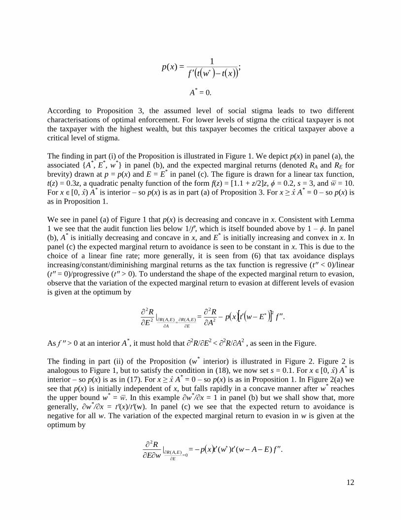
According to Proposition 3, the assumed level of social stigma leads to two different

characterisations of optimal enforcement. For lower levels of stigma the critical taxpayer is not

the taxpayer with the highest wealth, but this taxpayer becomes the critical taxpayer above a

critical level of stigma.

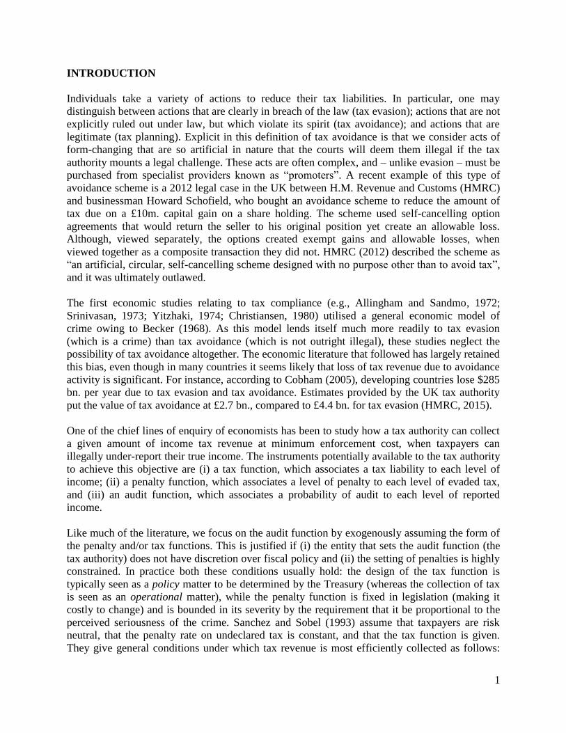
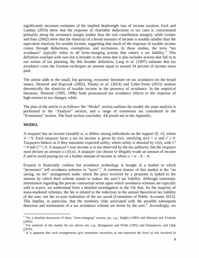
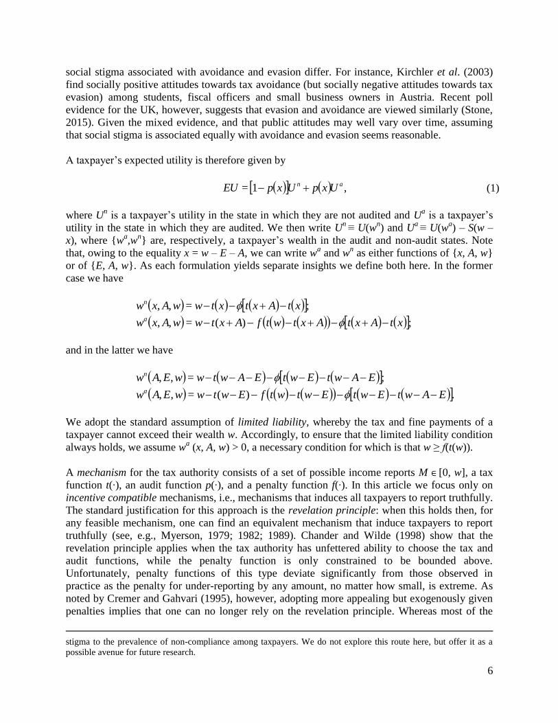
The finding in part (i) of the Proposition is illustrated in Figure 1. We depict p(x) in panel (a), the

associated {A*, E

*, w

*} in panel (b), and the expected marginal returns (denoted RA and RE for

brevity) drawn at p = p(x) and E = E* in panel (c). The figure is drawn for a linear tax function,

t(z) = 0.3z, a quadratic penalty function of the form f(z) = [1.1 + z/2]z, ϕ = 0.2, s = 3, and = 10.

For x ∈ [0, ) A* is interior – so p(x) is as in part (a) of Proposition 3. For x ≥ A

* = 0 – so p(x) is

as in Proposition 1.

We see in panel (a) of Figure 1 that p(x) is decreasing and concave in x. Consistent with Lemma

1 we see that the audit function lies below 1/fꞌ, which is itself bounded above by 1 – ϕ. In panel

(b), A* is initially decreasing and concave in x, and E

* is initially increasing and convex in x. In

panel (c) the expected marginal return to avoidance is seen to be constant in x. This is due to the

choice of a linear fine rate; more generally, it is seen from (6) that tax avoidance displays

increasing/constant/diminishing marginal returns as the tax function is regressive (tꞌꞌ < 0)/linear

(tꞌꞌ = 0)/progressive (tꞌꞌ > 0). To understand the shape of the expected marginal return to evasion,

observe that the variation of the expected marginal return to evasion at different levels of evasion

is given at the optimum by

.=|2

2

2

),(=

),(2

2

fEwtxpA

R

E

R

E

EAR

A

EAR

As f ꞌꞌ > 0 at an interior A*, it must hold that ∂

2R/∂E

2 < ∂

2R/∂A

2 , as seen in the Figure.

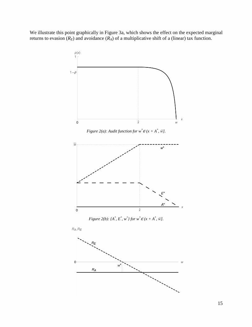
The finding in part (ii) of the Proposition (w* interior) is illustrated in Figure 2. Figure 2 is

analogous to Figure 1, but to satisfy the condition in (18), we now set s = 0.1. For x ∈ [0, ) A* is

interior – so p(x) is as in (17). For x ≥ A* = 0 – so p(x) is as in Proposition 1. In Figure 2(a) we

see that p(x) is initially independent of x, but falls rapidly in a concave manner after w* reaches

the upper bound w* = . In this example ∂w

*/∂x = 1 in panel (b) but we shall show that, more

generally, ∂w*/∂x = tꞌ(x)/tꞌ(w). In panel (c) we see that the expected return to avoidance is

negative for all w. The variation of the expected marginal return to evasion in w is given at the

optimum by

.)()(=|0=

),(

2

fEAwtwtxpwE

R

E

EAR

13

As fꞌꞌ > 0 at an interior w*, it must hold that ∂

2R/∂E∂w

<

0, as seen in the Figure.

Figure 1(a): Audit function for A*∈ (0, w

* – x].

Figure 1(b): {A*, E

*, w

*} for A

*∈ (0, w* – x].

14

Figure 1(c): Expected marginal return to avoidance and evasion for A*∈ (0, w

* – x)

We now formally investigate the comparative statics of the two cases analysed above:

Proposition 4 In an equilibrium in which either A* or w

* takes an interior value the comparative

statics of {A*, p(x), w

*} are given as in columns 3 and 4 of Table 1.

When A* takes an interior value the results in Table 1 (column 3) for the comparative statics of

p(x) are consistent with those obtained in Proposition 2: the audit function is a decreasing

function of declared income, shifts downwards with increases in ϕ and s, and shifts upwards in

. Moreover, ∂A*/∂x can be written as

,1<11

1=

fAxtww

xtf

x

Ahn

with the implication that E* is an increasing function of x (and A

*/E

* is a decreasing function of

x). Whether A*/E

* is an increasing or decreasing function of wealth depends on the shape of the

tax function. If the tax function is progressive or linear then it can be shown that ∂A*/∂ > 1, so

E* must fall, but both A

* and E

* may rise if the tax function is regressive.

When w* takes an interior value, however, the audit function becomes independent of declared

income (and this holds for any tax function). The audit function also becomes independent of

(as it is not predicated on the wealthiest taxpayer) and of ϕ (as avoidance is dominated by

evasion as a means of reducing tax liability). In both types of interior optimum a steepening of

the penalty function shifts the audit function downwards.

We now return to the question of the effects of a proportional increase in marginal tax rates (a

steepening of the tax function – again by means of an anti-clockwise pivot about the intercept).

Matching our finding in Proposition 2 for the case of a corner solution, the findings in Table 1

predict the opposite of the Yitzhaki (1974) finding: as marginal tax rates increase the tax

authority must shift upwards the audit function to maintain truthful reporting. This finding is of

note as Yitzhaki’s result is not only paradoxical intuitively, but much empirical and experimental

evidence finds a negative relationship between compliance and the tax rate (see, e.g., Bernasconi

et al., 2014, and the references therein).10

In interpreting this result it is of importance to note

that the Yitzhaki (1974) model can be augmented with a constant utility cost due to social stigma

– as in our model – without affecting the direction of the relationship between marginal tax rates

and non-compliance.11

This difference between models is not, therefore, a part of the

explanation of our differing findings. Rather, the reversal of Yitzhaki’s finding relies on the idea

that, even in cases where evasion becomes less attractive following an increase in marginal tax

rates, tax avoidance will become more attractive for sure. Thus the overall incentives for

non-compliance grow, even if the incentives for evasion weaken.

10

See also Piolatto and Rablen (2017) for a detailed analysis of Yitzhaki’s finding, and when it is and is not

overturned. 11

If, however, social stigma is viewed as a monetary, rather than utility cost, then a negative relationship between

compliance and the marginal tax rate can emerge in the Yitzhaki framework when the stigma cost is sufficiently

high (see, e.g., al-Nowaihi and Pyle, 2000).

15

We illustrate this point graphically in Figure 3a, which shows the effect on the expected marginal

returns to evasion (RE) and avoidance (RA) of a multiplicative shift of a (linear) tax function.

Figure 2(a): Audit function for w*∈ (x + A

*, ].

Figure 2(b): {A*, E

*, w

*} for w

*∈ (x + A*, ].

16

Figure 2(c): Expected marginal return to avoidance and evasion for w*∈ (x + A

*, ).

Specifically, we increase the marginal tax rate from t– = 0.2 to t

+ = 0.7 in the model specification

used in Figure 1. The increase in marginal tax rates is seen to increase the expected marginal

return to avoidance, so that the overall expected marginal return to non-compliance at the

optimum is increased (making p(x) higher).

Figure 3a: Effect of a multiplicative shift in the tax function on the expected marginal return to avoidance and

evasion – risk neutral case.

Figure 3b: Effect of a multiplicative shift in the tax function on the expected marginal return to avoidance and

evasion – risk aversion case (U(z) = z2/3

).

17

In this case the expected marginal return to evasion does not uniformly increase or decrease, but

rather evasion becomes subject to stronger diminishing marginal returns (recall that evasion and

avoidance are inversely related for a fixed x, so the amount of evasion increases from right to left

in Figure 3).

EXTENSIONS

In this Section we consider a range of realistic extensions to the model of the previous Section.

As, however, these extensions reduce (often substantially) the tractability of the model, we

proceed here with solved examples, rather than general analytic solutions. As a key feature of

our analysis is the incorporation of tax avoidance, we herein focus on the case in which the

incentive compatibility constraints bind for an interior level of avoidance.

Optimal Auditing

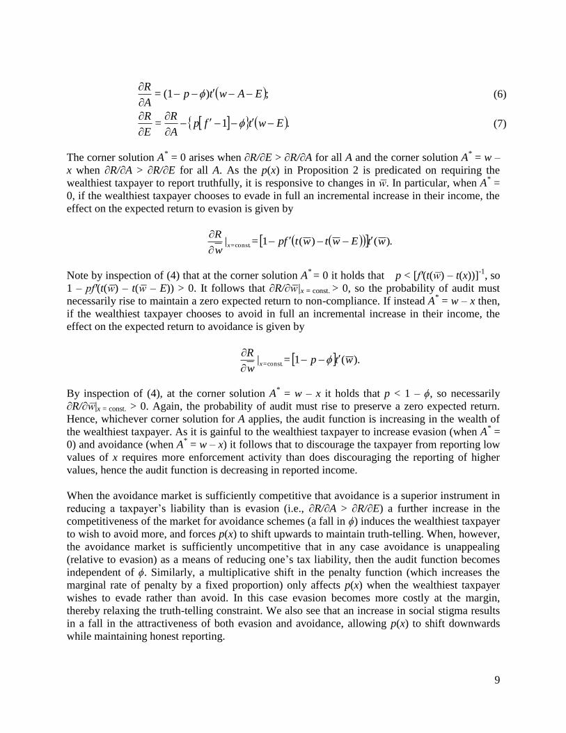
We now revisit the finding of Chander and Wilde (1998) that regressive tax functions are more

efficient than progressive tax functions (in the sense that they cost less to enforce). In Figure 4

we show p(x) for the linear (tꞌꞌ = 0), regressive (tꞌꞌ < 0), and progressive (tꞌꞌ > 0) cases.12

As in

previous Figures, A* is interior for x < and A

* = 0 for x ≥ . We see that the audit function in the

progressive case is everywhere above the audit function in the regressive case.

Figure 4: Audit function for a progressive, linear, and regressive tax function.

12

The specific functions depicted are t(x) = 0.3x (linear case); t(x) = 0.3x – 0.01x2 (regressive case); and t(x) =

0.06x2 (progressive case).

18

Hence, the model retains Chander and Wilde’s finding regarding the desirability of regressive

taxation from an enforcement cost perspective. Our finding is not importantly altered if we

instead employ the alternative formulation of the model whereby t(x + E) – t(x + E) is considered

the evaded tax and t(w) – t(w – A) is considered to be the avoided tax.

Risk Aversion

So far we have restricted the utility function to be linear. More generally, however, much

evidence points towards risk aversion, which implies a utility function satisfying Uꞌꞌ < 0. Figure

5 illustrates p(x) when taxpayers are risk neutral (U(x) = x) and when they are risk averse (U(x) =

x2/3

). The audit function under risk aversion is seen to lie everywhere below the equivalent

function when taxpayers are risk neutral. To understand this finding we apply Jensen’s inequality

to obtain

.1=1 nahna wxpSwxpUUUxpUxp

This inequality implies that wh ≤ p(x)[w

a –

S] + [1 – p(x)]w

n, which is equivalent to p(x) ≤ [w

n –

wh]/[w

n – w

a +

S]. Under risk neutrality this inequality binds, so p(x) must necessarily lie below

the risk neutral level when risk aversion is introduced.

Furthermore, the audit function under risk neutrality is steeper than under risk aversion. Under

risk neutrality an increase in declared income affects the taxpayer’s payoff by the difference

between the expected marginal return from truthful declaration and the expected marginal return

of the lottery associated with under-declaration. However, if the taxpayer is risk averse, the

expected marginal utility of an increase of x will also factor (positively) the reduction of risk.

Hence, in the risk aversion case, the audit function is less sensitive to increases in the amount

declared.

Figure 5: Effect of risk aversion.

19

Allowing for risk aversion – in particular, decreasing absolute risk aversion – also allows us to

demonstrate that the differences in findings in our model and the analysis of Yitzhaki continue to

pertain. In Figure 3b we observe that the tendency for avoidance to become more attractive after

a tax rate rise is more pronounced in the presence of risk aversion than without it.

Variable Social Stigma

We now relax the previous assumption of a constant utility cost of social stigma by allowing for

this cost to contain a variable component. We write

otherwise;0>

;= if0=

xws

wxxwS

where ψ ≥ 0. When ψ = 0 we recover the specification of S(∙) used in the previous Section.

Figure 6 compares the audit function in the two cases: one with a constant social stigma (s = 3, ψ

= 0) and one with variable stigma (s = 3, ψ = 0.9). As can be seen from the Figure, the increase

in ψ causes p(x) to shift downward and become flatter. While the first effect is due to the

absolute increase of the stigma cost, the second one is caused by variation in the marginal stigma

cost. Indeed, for a unitary increase of declared income x, the taxpayer reduces his stigma by an

amount ψ, hence, the reduction in the probability of audit following an increase x is smaller the

higher is ψ. In this way, holding the level of stigma constant, stiffer deterrence is needed when

the stigma cost is dependent on evaded liabilities so as to counteract the stigma-relieving effect

of an increase in the declaration.

Figure 6: Effect of a variable component to social stigma.

20

CONCLUSION

In this article we investigated how accounting for the ability of individuals to avoid tax, as well

as to evade tax, alters the conclusions for optimal auditing of models in which only tax evasion is

possible. The nature of the avoidance activity we consider is not explicitly prohibited by law, but

is unacceptable to the tax authority. Accordingly, if the tax authority learns of the avoidance, it

moves (successfully in our model) to outlaw it ex-post.

Some key features of the literature that considers only evasion are preserved: we find that the

audit function is a non-increasing function of declared income and, as in Chander and Wilde

(1998), less enforcement is required to enforce a regressive tax than to enforce a progressive tax.

The model does, however, also yield new insights, in particular around the relationship between

tax compliance and marginal tax rates. The evasion-only literature has encountered the so-called

“Yitzhaki puzzle” whereby stiffer marginal tax rates decrease incentives to be non-compliant. In

our framework, however, the opposite applies: incentives to be non-compliant increase with

marginal tax rates. The key to this result is that the incentives to avoid tax unambiguously

increase following an increase in marginal tax rates. Thus, even though the incentives for evasion

may worsen, nonetheless, the tax system becomes more costly to enforce, and overall

compliance falls unless enforcement is stiffened.

We are also able to understand further questions such as “which taxpayers are the most difficult

(expensive) to make compliant?”; and “should tax auditing be geared to preventing avoidance or

evasion?” On the first question, we find that in plausible circumstances it is the wealthiest

taxpayer who is the most difficult to make compliant. While we know of no direct empirical

evidence on this matter, our result chimes with the findings of attitudinal research regarding

perceptions of the compliance of the rich (e.g., Wallschutzky, 1984; Citrin, 1979). The answer to

the second question depends critically on (i) the level and shape of the penalties for evasion; and

(ii) the competitiveness of the market for avoidance schemes (for this determines the share of the

possible proceeds from avoidance that must be paid as a fee). If the penalty function is linear or

concave then, irrespective of the tax function, a non-compliant taxpayer will engage purely in

avoidance, or purely in evasion. Thus enforcement is focused entirely on one form of

non-compliance or the other. When, however, the penalty function is convex (which seems quite

likely empirically, given that smaller cases of tax evasion are typically punished through fines,

but larger cases are punished through prison sentences) a non-compliant taxpayer may

simultaneously want to avoid and evade tax, so enforcement must reflect both of these

possibilities. We have shown that a taxpayer’s preferred mix of avoidance and evasion moves in

favour of avoidance as reported income decreases, as the competitiveness of the market for

avoidance schemes increases, and as the social stigma associated with tax non-compliance falls.

We finish with some avenues for future research. First, it would be of interest to allow for

imperfect audit effectiveness, as in Rablen (2014) and Snow and Warren (2005a; 2005b), for it

might be that evasion and avoidance differ in the amount of tax inspector time required to detect

them. Second, it might also be of interest to model more carefully the market for avoidance. In

21

practice there are a range of providers of tax advice, ranging from those that offer solely tax

planning, to those that are willing to offer aggressive (or even criminal) methods, making it

important to understand the separate supply- and demand-side effects. A last suggestion is to

explore the effects of different forms of avoidance. We assume that avoidance permits some

amount of income to be hidden from the tax authority, but an alternative modelling approach

might be to assume that it allows some amount of income to be taxed at a lower rate.

REFERENCES

Allingham, M. G. and Sandmo, A. (1972). Income tax evasion: A theoretical analysis. Journal of

Public Economics, 1(3-4), pp. 323–338.

al-Nowaihi, A. and Pyle, D. (2000). Income tax evasion: a theoretical analysis. In A. MacDonald

and D. Pyle (eds.) Illicit Activity: The Economics of Crime and Tax Fraud. Aldershot:

Ashgate, pp. 249–266.

Alm, J. (1988). Compliance costs and the tax avoidance tax evasion decision. Public Finance

Quarterly, 16(1), pp. 31–66.

Alm, J., Bahl, R. and Murray, M. N. (1990). Tax structure and tax compliance. Review of

Economics and Statistics, 72(4), pp. 603–613.

Alm, J. and McCallin, N. J. (1990). Tax avoidance and tax evasion as a joint portfolio choice.

Public Finance / Finances Publiques, 45(2), pp. 193–200.

Baldry, J. C. (1986). Tax evasion is not a gamble. Economics Letters, 22(4), pp. 333–335.

Becker, G. S. (1968). Crime and punishment: An economic approach. Journal of Political

Economy, 76(2), pp. 169–217.

Benjamini, Y. and Maital, S. (1985). Optimal tax evasion and optimal tax evasion policy:

behavioural aspects. In W. Gaertner and A. Wenig (eds.) The Economics of the Shadow

Economy. Berlin: Springer-Verlag, pp. 245–264.

Bernasconi, M., Corazzini, L. and Seri, R. (2014). Reference dependent preferences, hedonic

adaptation and tax evasion: Does the tax burden matter? Journal of Economic Psychology,

40(1), pp. 103–118.

Chander, P. (2007). Income tax evasion and the fear of ruin. Economica, 74(294), pp. 315–328.

Chander, P. and Wilde, L. L. (1998). A general characterization of optimal income tax

enforcement. Review of Economic Studies, 65(1), pp. 165–183.

Chetty, R. (2009). Is the taxable income elasticity sufficient to calculate deadweight loss? The

implications of evasion and avoidance. American Economic Journal: Economic Policy,

22

1(2), pp. 31–52.

Christiansen, V. (1980). Two comments on tax evasion. Journal of Public Economics, 13(3), pp.

389–393.

Citrin, J. (1979). Do people want something for nothing: public opinion on taxes and public

spending. National Tax Journal, 32(2), pp. 113–129.

Cobham, A. (2005). Tax evasion, tax avoidance and development finance. QEH Working Paper

Series No. 129, University of Oxford.

Committee of Public Accounts (2013) Tax Avoidance: Tackling Marketed Avoidance Schemes.

London: The Stationery Office.

Cowell, F. A. (1990). Tax sheltering and the cost of evasion. Oxford Economic Papers, 42(1), pp.

231–243.

Cremer, H. and Gahvari, F. (1995). Tax evasion and the general income tax. Journal of Public

Economics, 60(2), pp. 235–249.

Damjanovic, T. and Ulph, D. (2010). Tax progressivity, income distribution and tax

non-compliance. European Economic Review, 54(4), pp. 594–607.

Dell’Anno, R. (2009). Tax evasion, tax morale and policy maker’s effectiveness. Journal of

Socio-Economics, 38(6), pp. 988–997.

Dhami, S. and al-Nowaihi, A. (2007). Why do people pay taxes: Expected utility theory versus

prospect theory. Journal of Economic Behavior and Organization, 64(1), pp. 171–192.

Erard, B. and Feinstein, J. (1994). Honesty and evasion in the tax compliance game. RAND

Journal of Economics, 25(1), pp. 1–19.

Feldstein, M. (1999). Tax avoidance and the deadweight loss of the income tax. Review of

Economics and Statistics, 81(4), pp. 674–680.

Fack, G. and Landais, C. (2010). Are tax incentives for charitable giving efficient? Evidence

from France. American Economic Journal: Economic Policy, 2(2), pp. 117–141.

Gruber, J. and Saez, E. (2002). The elasticity of taxable income: evidence and implications.

Journal of Public Economics, 84(1), pp. 1–32.

Gordon, J. P. F. (1989). Individual morality and reputation costs as deterrents to tax evasion.

European Economic Review, 33(4), pp. 797–805.

Hashimzade, N., Myles, G. D., Page, F. and Rablen, M. D. (2014). Social networks and

occupational choice: The endogenous formation of attitudes and beliefs about tax

23

compliance. Journal of Economic Psychology, 40(1), pp. 134–146.

Hashimzade, N., Myles, G. D., Page, F. and Rablen, M. D. (2015). The use of agent-based

modelling to investigate tax compliance. Economics of Governance, 16(2), pp. 143–164.

Hashimzade, N., Myles, G. D. and Rablen, M. D. (2016). Predictive analytics and the targeting

of audits. Journal of Economic Behavior and Organization, 124(1), pp. 130–145.

Hindriks, J. (1999). On the incompatibility between revenue maximisation and tax progressivity.

European Journal of Political Economy, 15(1), pp. 123–140.

HMRC (2012) Court of Appeal Backs HMRC in Tax Avoidance Case, NAT69/12, London: HM

Revenue and Customs.

HMRC (2015) Measuring Tax Gaps 2015 Edition: Tax Gap Estimates for 2013-14, London: HM

Revenue and Customs.

Kim, Y. (2003). Income distribution and equilibrium multiplicity in a stigma-based model of tax

evasion. Journal of Public Economics, 87(7-8), pp. 1591–1616.

Kirchler, E., Maciejovsky, B. and Schneider, F. (2003). Everyday representations of tax

avoidance, tax evasion, and tax flight: do legal differences matter? Journal of Economic

Psychology, 24(4), pp. 535–553.

Lang, O., Nöhrbaß , K. H. and Stahl, K. (1997). On income tax avoidance: the case of Germany.

Journal of Public Economics, 66(2), pp. 327–347.

Lee, K. (2001). Tax evasion and self-insurance. Journal of Public Economics, 81(1), pp. 73–81.

Marhuenda, F. and Ortuño-Ortín, I. (1994). Honesty vs. progressiveness in income tax

enforcement problems. Working paper no. 9406, University of Alicante.

Mookherjee, D. and Png, I. (1989). Optimal auditing, insurance, and redistribution. Quarterly

Journal of Economics, 104(2), pp. 399–415.

Morton, S. (1993). Strategic auditing for fraud. The Accounting Review, 68(4), pp. 825–839.

Myerson, R. B. (1979). Incentive compatibility and the bargaining problem. Econometrica,

47(1), pp. 61–74.

Myerson, R. B. (1982). Optimal coordination mechanisms in generalized principal-agent

problems. Journal of Mathematical Economics, 10(1), pp. 67–81.

Myerson, R. B. (1989). Mechanism design. In J. Eatwell, M. Milgate, and P. Newman (eds.)

Allocation, Information, and Markets. New York: Macmillan Press, pp. 191–206.

24

Myles, G. D. and Naylor, R. A. (1996). A model of tax evasion with group conformity and social

customs. European Journal of Political Economy, 12(1), pp. 49–66.

Piketty, T., Saez, E. and Stantcheva, S. (2014). Optimal taxation of top labor incomes: A tale of

three elasticities. American Economic Journal : Economic Policy, 6(1), pp. 230–271.

Piolatto, A. and Rablen, M. D. (2017). Prospect theory and tax evasion: A reconsideration of the

Yitzhaki puzzle. Theory and Decision, 82(4), pp. 543–565.

Rablen, M. D. (2014). Audit probability versus effectiveness: The Beckerian approach revisited.

Journal of Public Economic Theory, 16(2), pp. 322–342.

Reinganum, J. and Wilde, L. (1985). Income tax compliance in a principal-agent framework.

Journal of Public Economics, 26(1), pp. 1–18.

Reinganum, J. and Wilde, L. (1986). Equilibrium verification and reporting policies in a model

of tax compliance. International Economic Review, 27(3), pp. 739–760.

Reinganum, J. and Wilde, L. (1991). Equilibrium enforcement and compliance in the presence of

tax practitioners. Journal of Law, Economics & Organization, 7(1), pp. 163–181.

Sanchez, I. and Sobel, J. (1993). Hierarchical design and enforcement of income tax policies.

Journal of Public Economics, 50(3), pp. 345–369.

Scotchmer, S. (1987). Audit classes and tax enforcement policy. American Economic Review,

77(2), pp. 229–233.

Slemrod, J. (1995). Income creation or income shifting? Behavioral responses to the tax reform

act of 1986. American Economic Review, 85(2), pp. 175–180.

Slemrod, J. (1996). High-income families and the tax changes of the 1980s: The anatomy of

behavioral response. In M. Feldstein and J. M. Poterba (eds.) Empirical Foundations of

Household Taxation. Chicago: University of Chicago Press, pp. 169–192.

Slemrod, J. (2001). A general model of the behavioral response to taxation. International Tax and

Public Finance, 8(2), pp. 119–128.

Slemrod, J. and Yitzhaki, S. (2002). Tax avoidance, evasion and administration. In A. Auerbach

and M. Feldstein (eds.) Handbook of Public Economics. 1st Ed. Amsterdam:

North-Holland, pp. 1423–1470.

Slemrod, J. and Kopczuk, W. (2002). The optimal elasticity of taxable income. Journal of Public

Economics, 84(1), pp. 91–112.

Snow, A. and Warren Jr., R. S. (2005a). Ambiguity about audit probability, tax compliance, and

taxpayer welfare. Economic Inquiry, 43(4), pp. 865–871.

25

Snow, A. and Warren Jr., R. S. (2005b). Tax evasion under random audits with uncertain

detection. Economics Letters, 88(1), pp. 97–100.

Srinivasan, T. N. (1973). Tax evasion: A model. Journal of Public Economics, 2(4), pp.

339–346.

Stiglitz, J. E. (1985). The general theory of tax avoidance. National Tax Journal, 38(3), pp.

325–337.

Stone, J. (2015). Most people think legal tax avoidance is just as wrong as illegal tax evasion,

poll suggests. The Independent, 1 March 2015, London: Independent Print Limited.

Available at:

http://www.independent.co.uk/news/uk/politics/most-people-think-legal-tax-avoidance-is-j

ust-as-wrong-as-illegal-tax-evasion-10077934.html (Accessed: 10 October 2016)

Uribe-Teran, C. (2015). Down the rabbit-hole: Tax avoidance and the elasticity of taxable

income. Mimeo.

Wallschutzky, I. G. (1984). Possible causes of tax evasion. Journal of Economic Psychology,

5(4), pp. 371–384.

Yitzhaki, S. (1974). A note on 'Income tax evasion: A theoretical analysis'. Journal of Public

Economics, 3(2), pp. 201–202.

26

APPENDIX

Proof of Proposition 1: For each value of x, we wish to maximise p(x; A, w) in (3) with respect

to A and w (allowing the suppressed variable E to vary). First, maximising with respect to A, the

first order condition for a maximum is

.

1

1=

,;2

sxtxAtxAtwth

xAtxtwths

A

wAxp

(A.1)

Then (A.1) implies that A* = 0 when

,1

=ˆ>xtwths

xtwth

and A* = w – x when ϕ < . When ϕ = all feasible values of A weakly maximise p(x; A, w).

Taking the case ϕ > first, to find p(x) we now maximise p(x; 0, w) with respect to w. The first

derivative with respect to w is

,0>

1=

;0,2

sxtwth

wts

w

wxp

(A.2)

so w* = . In the case ϕ < the relevant first derivative with respect to w is

,0>

1=

,;2

sxtwt

wts

w

wxwxp

(A.3)

so again w* = .

Proof of Proposition 2: Differentiating in (4) we obtain that, if A* = 0, then

0;>1)w(

=)(

sf

fxpt

w

xp

0;<)w(1

=)(

sf

tfxp

x

xp

0;<=)(

sf

xp

s

xp

0;<=);(

sf

fxpfxp

27

0;>][1=),(

fxpxptxp

0.=)(

xp

The comparative statics when A* = w – x follow similarly.

Proof of Lemma 1: (i) We first prove p(x)fꞌ < 1 From (11), (13) and (15), if there exists a ≤

such that p(x; A, w) attains the value p(x; A, ) = [fꞌ(t( ) – t(x + A))]-1

then p(x; A, ) = maxw p(x;

A, w) – for if (10) defines a maximum in A, as assumed, then (10) defines a maximum in w. p(x;

A, ) is maximised in A when = 0 (as fꞌꞌ > 0 for there to be an interior A*), so ≠ w

* for, by

assumption, if it were that = w* then p(x; A, ) would be maximised for an interior value of A.

Hence we have [fꞌ(t( ) – t(x + A*))]

-1 > p(x; A

*, w

*) = p(x). As this will hold for every , we have

p(x)fꞌ < 1. If ∂p(x; A, w)/∂w > 0 everywhere then there does not exist a ≤ such that ∂p(x; A,

w)/∂w = 0. We note that it cannot be that ∂p(x; A, w)/∂w < 0 everywhere as ∂p(x; A, w)/∂w|A = w – x

= 0 = ϕ tꞌ(x)/[s + f(0)] > 0. In this case p(x; A, w) is maximised at w = and satisfies p(x; A, ) <

[fꞌ(t( ) – t(x + A))]-1

. An analogous argument to that above then establishes that p(x)fꞌ < 1. Then,

from (12), we may set p(x) = ϕ[fꞌ – 1]-1

in p(x)fꞌ < 1 to obtain [1 – ϕ] fꞌ > 1. That p(x) < 1 – ϕ

follows immediately. Part (ii) follows by similar arguments.

Proof of Proposition 3: Using (10), the effect of w on p(x; A, w) when ∂p(x; A, w)/∂A = 0 is

given by

0;>

),;(1=|

),;(

0=),;(

sww

wtwAxp

w

wAxpan

A

wAxp

where the inequality follows from Lemma 1. This implies that when A* is interior, w

* is

maximal. Substituting w = in (12) we therefore obtain

.1

=)( Axtwtf

xp

From (10) and Lemma 1 we have

0.>=)(1

AxtwtfxtAxtAxtwtfs

AxtwtfAxtwtAxtwtfsxp

Hence, it must hold that s > εf (t( ) – t(x+A*)) – 1, where εf (z) = zfꞌ (z)/f (z) is the elasticity of the

penalty function with respect to evaded tax, so interior values of A* arise for sufficiently high

social stigma costs.

Using (11), the effect of A on p(x; A, w) when ∂p(x; A, w)/∂w = 0 is given by

28

.0<),;(1=|),;(

0=),;( AxtwAxp

A

wAxp

w

wAxp

This implies that when w* is interior, A

* takes its minimum possible value of zero. Substituting A

= 0 in (13) we therefore obtain

.1

=)(xtwtf

xp

From (11) we have

0.<1=)(1

xtwtfs

xtwtfxtwtxp

(A. 4)

As (A. 4) is negative, it must be that s < εf (t(w*) – t(x)) – 1. Hence, w

* is interior when a

sufficiently low level of social stigma prevails, whereas A* is interior when a sufficiently high

level of social stigma prevails.

Proof of Proposition 4: The comparative statics of a pivot around (z, f(z)) = (0, 0) are found by

writing f(∙) as εf(∙), differentiating with respect to ε, and then examining the resulting derivative

as ε → 1. The pivot of the tax function is performed analogously. The comparative statics of a

shift of the tax function are found by replacing t(∙) with t(∙) + ε, differentiating with respect to ε,

and then examining the resulting derivative as ε → 0. When A*∈ (0, w – x) we use the implicit

function theorem in (10) to obtain:

0;<)(= xAtsgns

Asgn

0;<)]()([= sfxtxAtfsgnA

sgn

0;>][1][1= fwwfsgnw

Asgn hn

0;<))(][)(1][1(= fxAtwwxtfsgnx

Asgn hn

0;>))()((=)(

xtwtssgnfA

sgn

29

0;>)]()w(1}[]{[1])][()(([=)(

xttffwwxAtwtsgntA

sgn hn

and when w*∈ (x, x + A) we use the IFT in (11) to obtain

0;>)(=

wtsgn

s

wsgn

0;<][

)(=

)(2

sf

wtssgn

fwsgn

0;>)(

)(=

wt

xtsgn

x

wsgn

;0=0=w

sgnw

sgn

0;<

)(=

)(2

f

wtfsgn

twsgn

0.=(0)= sgnw

sgn

Turning to p(x), we use the IFT in (2) along with (10) or (11) to obtain

0;<)(=)( hn wwsgn

s

xpsgn

0;<)]([=);(

fwwsgnfxp

sgn hn

;, if0=(0)

;0, if 0<)(1

=)(

Axxwsgn

xwAsww

xpsgn

x

xpsgn cn

;, if0=(0)

;0, if0>1})]({[1=

)(

Axxwsgn

xwAfsgn

w

xpsgn

30

;, if0=(0)

;0, if0>1)]([1=

);(

Axxwsgn

xwAfsgntxpsgn

;, if0=(0)

;0, if0<1][1=

)(

Axxwsgn

xwAfsgnxpsgn

31

Tables

Table 1: Comparative statics.

0=A xwA = xwA 0, wAxw ,

)(xp )(xp A )(xp w )(xp

x 0

w 0 0

0 0 0

s

pivot of f(∙) 0

pivot of t(∙) 0