Taurus™ TSUPREM-4™ User GuideVersion N-2017.09, September 2017

ii Taurus™ TSUPREM-4™ User GuideN-2017.09

Copyright and Proprietary Information Notice© 2017 Synopsys, Inc. This Synopsys software and all associated documentation are proprietary to Synopsys, Inc. and may only be used pursuant to the terms and conditions of a written license agreement with Synopsys, Inc. All other use, reproduction, modification, or distribution of the Synopsys software or the associated documentation is strictly prohibited.

Destination Control StatementAll technical data contained in this publication is subject to the export control laws of the United States of America. Disclosure to nationals of other countries contrary to United States law is prohibited. It is the reader’s responsibility to determine the applicable regulations and to comply with them.

DisclaimerSYNOPSYS, INC., AND ITS LICENSORS MAKE NO WARRANTY OF ANY KIND, EXPRESS OR IMPLIED, WITH REGARD TO THIS MATERIAL, INCLUDING, BUT NOT LIMITED TO, THE IMPLIED WARRANTIES OF MERCHANTABILITY AND FITNESS FOR A PARTICULAR PURPOSE.

TrademarksSynopsys and certain Synopsys product names are trademarks of Synopsys, as set forth athttps://www.synopsys.com/company/legal/trademarks-brands.html.All other product or company names may be trademarks of their respective owners.

Third-Party LinksAny links to third-party websites included in this document are for your convenience only. Synopsys does not endorse and is not responsible for such websites and their practices, including privacy practices, availability, and content.

Synopsys, Inc.690 E. Middlefield RoadMountain View, CA 94043www.synopsys.com

CONTENTS

Contents

About This Guide xxv

Overview. . . . . . . . . . . . . . . . . . . . . . . . . . . . . . . . . . . . . . . . . . . . . . . . . xxvRelated Publications . . . . . . . . . . . . . . . . . . . . . . . . . . . . . . . . . . . . . . . xxvi

Reference Materials . . . . . . . . . . . . . . . . . . . . . . . . . . . . . . . . . . . . . xxviConventions . . . . . . . . . . . . . . . . . . . . . . . . . . . . . . . . . . . . . . . . . . . . . xxviCustomer Support . . . . . . . . . . . . . . . . . . . . . . . . . . . . . . . . . . . . . . . . . xxvii

Accessing SolvNet . . . . . . . . . . . . . . . . . . . . . . . . . . . . . . . . . . . . . . xxviiContacting the Synopsys Technical Support Center . . . . . . . . . . . xxviiiContacting Your Local TCAD Support Team Directly . . . . . . . . . xxviii

Chapter 1: Introduction to TSUPREM-4 1-1

Product Name Change . . . . . . . . . . . . . . . . . . . . . . . . . . . . . . . . . . . . . . 1-1Program Overview . . . . . . . . . . . . . . . . . . . . . . . . . . . . . . . . . . . . . . . . . 1-1Processing Steps . . . . . . . . . . . . . . . . . . . . . . . . . . . . . . . . . . . . . . . . . . . 1-2Simulation Structure . . . . . . . . . . . . . . . . . . . . . . . . . . . . . . . . . . . . . . . . 1-2Additional Features. . . . . . . . . . . . . . . . . . . . . . . . . . . . . . . . . . . . . . . . . 1-2

Chapter 2: Using TSUPREM-4 2-1

Program Execution and Output. . . . . . . . . . . . . . . . . . . . . . . . . . . . . . . . 2-1Starting TSUPREM-4 . . . . . . . . . . . . . . . . . . . . . . . . . . . . . . . . . . . . 2-1Program Output . . . . . . . . . . . . . . . . . . . . . . . . . . . . . . . . . . . . . . . . . 2-2

Printed Output . . . . . . . . . . . . . . . . . . . . . . . . . . . . . . . . . . . . . . . . 2-2Graphical Output . . . . . . . . . . . . . . . . . . . . . . . . . . . . . . . . . . . . . . 2-2

Errors, Warnings, and Syntax . . . . . . . . . . . . . . . . . . . . . . . . . . . . . . 2-3File Specification . . . . . . . . . . . . . . . . . . . . . . . . . . . . . . . . . . . . . . . . . . 2-3

File Types. . . . . . . . . . . . . . . . . . . . . . . . . . . . . . . . . . . . . . . . . . . . . . 2-3Default File Names . . . . . . . . . . . . . . . . . . . . . . . . . . . . . . . . . . . . . . 2-3Environment Variables . . . . . . . . . . . . . . . . . . . . . . . . . . . . . . . . . . . 2-4

Taurus™ TSUPREM-4™ User Guide iiiN-2017.09

Contents

Input Files . . . . . . . . . . . . . . . . . . . . . . . . . . . . . . . . . . . . . . . . . . . . . . . . 2-4Command Input Files. . . . . . . . . . . . . . . . . . . . . . . . . . . . . . . . . . . . . 2-4Mask Data Files . . . . . . . . . . . . . . . . . . . . . . . . . . . . . . . . . . . . . . . . . 2-5Profile Files . . . . . . . . . . . . . . . . . . . . . . . . . . . . . . . . . . . . . . . . . . . . 2-5Other Input Files . . . . . . . . . . . . . . . . . . . . . . . . . . . . . . . . . . . . . . . . 2-5

Output Files. . . . . . . . . . . . . . . . . . . . . . . . . . . . . . . . . . . . . . . . . . . . . . . 2-5Terminal Output . . . . . . . . . . . . . . . . . . . . . . . . . . . . . . . . . . . . . . . . . 2-6Output Listing Files . . . . . . . . . . . . . . . . . . . . . . . . . . . . . . . . . . . . . . 2-6

Standard Output File—s4out. . . . . . . . . . . . . . . . . . . . . . . . . . . . . 2-6Informational Output File—s4inf . . . . . . . . . . . . . . . . . . . . . . . . . 2-6Diagnostic Output File—s4dia . . . . . . . . . . . . . . . . . . . . . . . . . . . 2-6

Saved Structure Files . . . . . . . . . . . . . . . . . . . . . . . . . . . . . . . . . . . . . 2-7TSUPREM-4 . . . . . . . . . . . . . . . . . . . . . . . . . . . . . . . . . . . . . . . . . 2-7TIF. . . . . . . . . . . . . . . . . . . . . . . . . . . . . . . . . . . . . . . . . . . . . . . . . 2-7Medici . . . . . . . . . . . . . . . . . . . . . . . . . . . . . . . . . . . . . . . . . . . . . . 2-7MINIMOS 5 . . . . . . . . . . . . . . . . . . . . . . . . . . . . . . . . . . . . . . . . . 2-7Wave . . . . . . . . . . . . . . . . . . . . . . . . . . . . . . . . . . . . . . . . . . . . . . . 2-7

Graphical Output . . . . . . . . . . . . . . . . . . . . . . . . . . . . . . . . . . . . . . . . 2-7Extract Output Files . . . . . . . . . . . . . . . . . . . . . . . . . . . . . . . . . . . . . . 2-8Electrical Data Output Files . . . . . . . . . . . . . . . . . . . . . . . . . . . . . . . . 2-8

Library Files . . . . . . . . . . . . . . . . . . . . . . . . . . . . . . . . . . . . . . . . . . . . . . 2-8Initialization Input File—s4init . . . . . . . . . . . . . . . . . . . . . . . . . . . . . 2-9Ion Implant Data File—s4imp0 . . . . . . . . . . . . . . . . . . . . . . . . . . . . . 2-9Ion Implant Damage Data File—s4idam . . . . . . . . . . . . . . . . . . . . . . 2-9Plot Device Definition File—s4pcap . . . . . . . . . . . . . . . . . . . . . . . . 2-10Key Files—s4fky0 and s4uky0 . . . . . . . . . . . . . . . . . . . . . . . . . . . . 2-10Authorization File—s4auth . . . . . . . . . . . . . . . . . . . . . . . . . . . . . . . 2-10

Chapter 3: TSUPREM-4 Models 3-1

Simulation Structure . . . . . . . . . . . . . . . . . . . . . . . . . . . . . . . . . . . . . . . . 3-2Coordinates . . . . . . . . . . . . . . . . . . . . . . . . . . . . . . . . . . . . . . . . . . . . 3-2Initial Structure . . . . . . . . . . . . . . . . . . . . . . . . . . . . . . . . . . . . . . . . . 3-2Regions and Materials . . . . . . . . . . . . . . . . . . . . . . . . . . . . . . . . . . . . 3-2

Grid Structure . . . . . . . . . . . . . . . . . . . . . . . . . . . . . . . . . . . . . . . . . . . . . 3-3Mesh, Triangular Elements, and Nodes . . . . . . . . . . . . . . . . . . . . . . . 3-3Defining Grid Structure . . . . . . . . . . . . . . . . . . . . . . . . . . . . . . . . . . . 3-3Explicit Specification of Grid Structure. . . . . . . . . . . . . . . . . . . . . . . 3-3

The LINE Statement . . . . . . . . . . . . . . . . . . . . . . . . . . . . . . . . . . . 3-4Generated Grid Lines . . . . . . . . . . . . . . . . . . . . . . . . . . . . . . . . . . 3-4Eliminating Grid Lines . . . . . . . . . . . . . . . . . . . . . . . . . . . . . . . . . 3-5

Automatic Grid Generation . . . . . . . . . . . . . . . . . . . . . . . . . . . . . . . . 3-5Automatic Grid Generation in the X-Direction. . . . . . . . . . . . . . . 3-6Automatic Grid Generation in the Y-Direction. . . . . . . . . . . . . . . 3-7

Changes to the Mesh During Processing . . . . . . . . . . . . . . . . . . . . . . 3-7DEPOSITION and EPITAXY . . . . . . . . . . . . . . . . . . . . . . . . . . . 3-7

iv Taurus™ TSUPREM-4™ User GuideN-2017.09

Contents

TN

Structure Extension . . . . . . . . . . . . . . . . . . . . . . . . . . . . . . . . . . . . 3-8ETCH and DEVELOP . . . . . . . . . . . . . . . . . . . . . . . . . . . . . . . . . 3-8Oxidation and Silicidation. . . . . . . . . . . . . . . . . . . . . . . . . . . . . . . 3-9

Adaptive Gridding . . . . . . . . . . . . . . . . . . . . . . . . . . . . . . . . . . . . . . 3-10Refinement . . . . . . . . . . . . . . . . . . . . . . . . . . . . . . . . . . . . . . . . . 3-10Unrefinement. . . . . . . . . . . . . . . . . . . . . . . . . . . . . . . . . . . . . . . . 3-11Adaptive Gridding for Damage. . . . . . . . . . . . . . . . . . . . . . . . . . 3-12Usage. . . . . . . . . . . . . . . . . . . . . . . . . . . . . . . . . . . . . . . . . . . . . . 3-12

1-D Simulation of Simple Structures . . . . . . . . . . . . . . . . . . . . . . . . 3-13Initial Impurity Concentration . . . . . . . . . . . . . . . . . . . . . . . . . . . . . 3-13

Diffusion . . . . . . . . . . . . . . . . . . . . . . . . . . . . . . . . . . . . . . . . . . . . . . . . 3-14DIFFUSION Statement . . . . . . . . . . . . . . . . . . . . . . . . . . . . . . . . . . 3-15

Temperature . . . . . . . . . . . . . . . . . . . . . . . . . . . . . . . . . . . . . . . . 3-15Ambient Gas Pressure . . . . . . . . . . . . . . . . . . . . . . . . . . . . . . . . . 3-15Ambient Gas Characteristics. . . . . . . . . . . . . . . . . . . . . . . . . . . . 3-15Ambients and Oxidation of Materials . . . . . . . . . . . . . . . . . . . . . 3-16Default Ambients . . . . . . . . . . . . . . . . . . . . . . . . . . . . . . . . . . . . 3-16Chlorine. . . . . . . . . . . . . . . . . . . . . . . . . . . . . . . . . . . . . . . . . . . . 3-17Chemical Predeposition. . . . . . . . . . . . . . . . . . . . . . . . . . . . . . . . 3-17Solution of Diffusion Equations . . . . . . . . . . . . . . . . . . . . . . . . . 3-17

Diffusion of Impurities. . . . . . . . . . . . . . . . . . . . . . . . . . . . . . . . . . . 3-18Impurity Fluxes . . . . . . . . . . . . . . . . . . . . . . . . . . . . . . . . . . . . . . 3-18Mobile Impurities and Ion Pairing . . . . . . . . . . . . . . . . . . . . . . . 3-19Electric Field . . . . . . . . . . . . . . . . . . . . . . . . . . . . . . . . . . . . . . . . 3-20Diffusivities. . . . . . . . . . . . . . . . . . . . . . . . . . . . . . . . . . . . . . . . . 3-22

Point Defect Enhancement. . . . . . . . . . . . . . . . . . . . . . . . . . . . . . . . 3-24PD.FERMI Model . . . . . . . . . . . . . . . . . . . . . . . . . . . . . . . . . . . . 3-24PD.TRANS and PD.FULL Models. . . . . . . . . . . . . . . . . . . . . . . 3-25Paired Fractions of Dopant Atoms . . . . . . . . . . . . . . . . . . . . . . . 3-265-Stream Diffusion Model . . . . . . . . . . . . . . . . . . . . . . . . . . . . . 3-26Initialization of Pairs . . . . . . . . . . . . . . . . . . . . . . . . . . . . . . . . . . 3-27Boundary Conditions for Pairs . . . . . . . . . . . . . . . . . . . . . . . . . . 3-27Reaction Rate Constants . . . . . . . . . . . . . . . . . . . . . . . . . . . . . . . 3-31

Activation of Impurities . . . . . . . . . . . . . . . . . . . . . . . . . . . . . . . . . . 3-35Physical Mechanisms . . . . . . . . . . . . . . . . . . . . . . . . . . . . . . . . . 3-35Activation Models . . . . . . . . . . . . . . . . . . . . . . . . . . . . . . . . . . . . 3-35Model Details . . . . . . . . . . . . . . . . . . . . . . . . . . . . . . . . . . . . . . . 3-36Solid Solubility Model . . . . . . . . . . . . . . . . . . . . . . . . . . . . . . . . 3-37Solid Solubility Tables . . . . . . . . . . . . . . . . . . . . . . . . . . . . . . . . 3-37Dopant Clustering Model . . . . . . . . . . . . . . . . . . . . . . . . . . . . . . 3-38Pressure-Dependent Equilibrium Model. . . . . . . . . . . . . . . . . . . 3-38Transient Clustering Model. . . . . . . . . . . . . . . . . . . . . . . . . . . . . 3-38Dopant-Interstitial Clustering Model . . . . . . . . . . . . . . . . . . . . . 3-39Dopant-Vacancy Clustering Model. . . . . . . . . . . . . . . . . . . . . . . 3-40Full Dynamics of Dopant-Defect Clustering . . . . . . . . . . . . . . . 3-40Transient Precipitation Model. . . . . . . . . . . . . . . . . . . . . . . . . . . 3-59DDC and Precipitation Initialization. . . . . . . . . . . . . . . . . . . . . . 3-60

aurus™ TSUPREM-4™ User Guide v-2017.09

Contents

Initialization for In-Situ Doping . . . . . . . . . . . . . . . . . . . . . . . . . 3-63Segregation of Impurities. . . . . . . . . . . . . . . . . . . . . . . . . . . . . . . . . 3-63

Segregation Flux . . . . . . . . . . . . . . . . . . . . . . . . . . . . . . . . . . . . . 3-63Interface Trap Model . . . . . . . . . . . . . . . . . . . . . . . . . . . . . . . . . . . . 3-64

Using the Interface Trap Model . . . . . . . . . . . . . . . . . . . . . . . . . 3-67Dose Loss Model . . . . . . . . . . . . . . . . . . . . . . . . . . . . . . . . . . . . . . . 3-67Diffusion of Point Defects . . . . . . . . . . . . . . . . . . . . . . . . . . . . . . . . 3-68

Equilibrium Concentrations . . . . . . . . . . . . . . . . . . . . . . . . . . . . 3-68Charge State Fractions . . . . . . . . . . . . . . . . . . . . . . . . . . . . . . . . 3-69Point Defect Diffusion Equations . . . . . . . . . . . . . . . . . . . . . . . . 3-70Interstitial and Vacancy Diffusivities . . . . . . . . . . . . . . . . . . . . . 3-72Reaction of Pairs With Point Defects . . . . . . . . . . . . . . . . . . . . . 3-73Recombination of Interstitials With Vacancies. . . . . . . . . . . . . . 3-74Absorption by Traps, Clusters, and Dislocation Loops . . . . . . . 3-76

Injection and Recombination of Point Defects at Interfaces . . . . . . 3-76Surface Recombination Velocity Models . . . . . . . . . . . . . . . . . . 3-76Trapped Nitrogen–Dependent Surface Recombination . . . . . . . 3-78Injection Rate . . . . . . . . . . . . . . . . . . . . . . . . . . . . . . . . . . . . . . . 3-78Moving-Boundary Flux. . . . . . . . . . . . . . . . . . . . . . . . . . . . . . . . 3-79

Interstitial Traps . . . . . . . . . . . . . . . . . . . . . . . . . . . . . . . . . . . . . . . . 3-80Enabling, Disabling, and Initialization . . . . . . . . . . . . . . . . . . . . 3-80

Interstitial Clustering Models. . . . . . . . . . . . . . . . . . . . . . . . . . . . . . 3-811-Moment Clustering Model. . . . . . . . . . . . . . . . . . . . . . . . . . . . 3-812-Moment Interstitial Clustering Model . . . . . . . . . . . . . . . . . . . 3-84Equilibrium Small Clustering . . . . . . . . . . . . . . . . . . . . . . . . . . . 3-87Transient Small Clustering . . . . . . . . . . . . . . . . . . . . . . . . . . . . . 3-88

Vacancy Clustering Models . . . . . . . . . . . . . . . . . . . . . . . . . . . . . . . 3-90Large Clustering Model . . . . . . . . . . . . . . . . . . . . . . . . . . . . . . . 3-90Equilibrium Small Clustering . . . . . . . . . . . . . . . . . . . . . . . . . . . 3-92Transient Small Clustering . . . . . . . . . . . . . . . . . . . . . . . . . . . . . 3-93

Initialization of Large Point-Defect Clusters . . . . . . . . . . . . . . . . . . 3-95Dislocation Loop Model . . . . . . . . . . . . . . . . . . . . . . . . . . . . . . . . . 3-97

Equations for Dislocation Loop Model. . . . . . . . . . . . . . . . . . . . 3-97Loop Density Specified by L.DENS. . . . . . . . . . . . . . . . . . . . . . 3-98Loop Density Specified by L.THRESH . . . . . . . . . . . . . . . . . . . 3-98Evolution of Loops . . . . . . . . . . . . . . . . . . . . . . . . . . . . . . . . . . . 3-99Effects of Dislocation Loops. . . . . . . . . . . . . . . . . . . . . . . . . . . . 3-99

Oxidation . . . . . . . . . . . . . . . . . . . . . . . . . . . . . . . . . . . . . . . . . . . . . . . 3-99Theory of Oxidation. . . . . . . . . . . . . . . . . . . . . . . . . . . . . . . . . . . . 3-100Analytical Oxidation Models . . . . . . . . . . . . . . . . . . . . . . . . . . . . . 3-101

Overview . . . . . . . . . . . . . . . . . . . . . . . . . . . . . . . . . . . . . . . . . . 3-101Usage. . . . . . . . . . . . . . . . . . . . . . . . . . . . . . . . . . . . . . . . . . . . . 3-104The ERFC Model . . . . . . . . . . . . . . . . . . . . . . . . . . . . . . . . . . . 3-104ERF1, ERF2, and ERFG Models . . . . . . . . . . . . . . . . . . . . . . . 3-105

Numerical Oxidation Models. . . . . . . . . . . . . . . . . . . . . . . . . . . . . 3-107Oxide Growth Rate . . . . . . . . . . . . . . . . . . . . . . . . . . . . . . . . . . 3-107VERTICAL Model . . . . . . . . . . . . . . . . . . . . . . . . . . . . . . . . . . 3-110

vi Taurus™ TSUPREM-4™ User GuideN-2017.09

Contents

TN

COMPRESS Model. . . . . . . . . . . . . . . . . . . . . . . . . . . . . . . . . . 3-110VISCOUS Model . . . . . . . . . . . . . . . . . . . . . . . . . . . . . . . . . . . 3-112VISCOELA Model . . . . . . . . . . . . . . . . . . . . . . . . . . . . . . . . . . 3-114Anisotropic Stress-Dependent Reaction . . . . . . . . . . . . . . . . . . 3-119Strength-Limited Stress. . . . . . . . . . . . . . . . . . . . . . . . . . . . . . . 3-119

Polysilicon Oxidation. . . . . . . . . . . . . . . . . . . . . . . . . . . . . . . . . . . 3-119Surface Tension and Reflow . . . . . . . . . . . . . . . . . . . . . . . . . . . . . 3-119N2O Oxidation. . . . . . . . . . . . . . . . . . . . . . . . . . . . . . . . . . . . . . . . 3-120

Nitrogen Trap and Generation. . . . . . . . . . . . . . . . . . . . . . . . . . 3-120Surface Reaction Rate . . . . . . . . . . . . . . . . . . . . . . . . . . . . . . . . 3-121Thin Oxidation Rate . . . . . . . . . . . . . . . . . . . . . . . . . . . . . . . . . 3-121

Boron Diffusion Enhancement in Oxides . . . . . . . . . . . . . . . . . . . 3-121Diffusion Enhancement in Thin Oxides . . . . . . . . . . . . . . . . . . 3-122Diffusion Enhancement Due to Fluorine . . . . . . . . . . . . . . . . . 3-124

Silicide Models . . . . . . . . . . . . . . . . . . . . . . . . . . . . . . . . . . . . . . . . . . 3-124TiSi2 Growth Kinetics . . . . . . . . . . . . . . . . . . . . . . . . . . . . . . . . . . 3-125

Reaction at TiSi2/Si Interface . . . . . . . . . . . . . . . . . . . . . . . . . . 3-125Diffusion of Silicon. . . . . . . . . . . . . . . . . . . . . . . . . . . . . . . . . . 3-125Reaction at TiSi2/Si Interface . . . . . . . . . . . . . . . . . . . . . . . . . . 3-125Oxygen Dependence . . . . . . . . . . . . . . . . . . . . . . . . . . . . . . . . . 3-125Initialization . . . . . . . . . . . . . . . . . . . . . . . . . . . . . . . . . . . . . . . 3-126Material Flow . . . . . . . . . . . . . . . . . . . . . . . . . . . . . . . . . . . . . . 3-126

Impurities and Point Defects . . . . . . . . . . . . . . . . . . . . . . . . . . . . . 3-126Specifying Silicide Models and Parameters. . . . . . . . . . . . . . . . . . 3-126

Materials . . . . . . . . . . . . . . . . . . . . . . . . . . . . . . . . . . . . . . . . . . 3-127Impurities . . . . . . . . . . . . . . . . . . . . . . . . . . . . . . . . . . . . . . . . . 3-127Reactions . . . . . . . . . . . . . . . . . . . . . . . . . . . . . . . . . . . . . . . . . . 3-127Dopants . . . . . . . . . . . . . . . . . . . . . . . . . . . . . . . . . . . . . . . . . . . 3-129

Tungsten, Cobalt, and Nickel Silicide Models . . . . . . . . . . . . . . . 3-129Other Silicides . . . . . . . . . . . . . . . . . . . . . . . . . . . . . . . . . . . . . . . . 3-130

Stress Models . . . . . . . . . . . . . . . . . . . . . . . . . . . . . . . . . . . . . . . . . . . 3-130Stress History Model . . . . . . . . . . . . . . . . . . . . . . . . . . . . . . . . . . . 3-130Thermal Stress Model Equations . . . . . . . . . . . . . . . . . . . . . . . . . . 3-130

Boundary Conditions. . . . . . . . . . . . . . . . . . . . . . . . . . . . . . . . . 3-130Initial Conditions. . . . . . . . . . . . . . . . . . . . . . . . . . . . . . . . . . . . 3-131Intrinsic Stress in Deposited Layers . . . . . . . . . . . . . . . . . . . . . 3-131Effect of Etching and Depositional Stress. . . . . . . . . . . . . . . . . 3-132Using the Stress History Model . . . . . . . . . . . . . . . . . . . . . . . . 3-132Limitations . . . . . . . . . . . . . . . . . . . . . . . . . . . . . . . . . . . . . . . . 3-132

Dopant-Induced Stress Models . . . . . . . . . . . . . . . . . . . . . . . . . . . 3-133Dopant-Induced Stress During Deposition . . . . . . . . . . . . . . . . 3-134Dopant-Induced Stress During Diffusion . . . . . . . . . . . . . . . . . 3-134

Ion Implantation . . . . . . . . . . . . . . . . . . . . . . . . . . . . . . . . . . . . . . . . . 3-134Analytic Ion Implant Models . . . . . . . . . . . . . . . . . . . . . . . . . . . . . 3-135

Implanted Impurity Distributions . . . . . . . . . . . . . . . . . . . . . . . 3-135Implant Moment Tables . . . . . . . . . . . . . . . . . . . . . . . . . . . . . . 3-136Gaussian Distribution . . . . . . . . . . . . . . . . . . . . . . . . . . . . . . . . 3-138

aurus™ TSUPREM-4™ User Guide vii-2017.09

Contents

Pearson Distribution . . . . . . . . . . . . . . . . . . . . . . . . . . . . . . . . . 3-138Dual Pearson Distribution . . . . . . . . . . . . . . . . . . . . . . . . . . . . . 3-139Dose-Dependent Implant Profiles . . . . . . . . . . . . . . . . . . . . . . . 3-140Tilt and Rotation Tables . . . . . . . . . . . . . . . . . . . . . . . . . . . . . . 3-141Multilayer Implants . . . . . . . . . . . . . . . . . . . . . . . . . . . . . . . . . . 3-142Lateral Distribution . . . . . . . . . . . . . . . . . . . . . . . . . . . . . . . . . . 3-142Depth-Dependent Lateral Distribution . . . . . . . . . . . . . . . . . . . 3-143Dose Integration From Lateral Distribution . . . . . . . . . . . . . . . 3-143Wafer Tilt and Rotation. . . . . . . . . . . . . . . . . . . . . . . . . . . . . . . 3-143BF2 Implant. . . . . . . . . . . . . . . . . . . . . . . . . . . . . . . . . . . . . . . . 3-144Analytic Damage Model . . . . . . . . . . . . . . . . . . . . . . . . . . . . . . 3-144Taurus Analytic Implant Model . . . . . . . . . . . . . . . . . . . . . . . . 3-145

MC Ion Implant Model . . . . . . . . . . . . . . . . . . . . . . . . . . . . . . . . . 3-147Old TSUPREM-4 MC Model . . . . . . . . . . . . . . . . . . . . . . . . . . 3-147Taurus MC Implant . . . . . . . . . . . . . . . . . . . . . . . . . . . . . . . . . . 3-148Binary Scattering Theory . . . . . . . . . . . . . . . . . . . . . . . . . . . . . 3-150Amorphous Implant Calculation . . . . . . . . . . . . . . . . . . . . . . . . 3-154Electronic Stopping . . . . . . . . . . . . . . . . . . . . . . . . . . . . . . . . . . 3-156Damage Accumulation and De-Channeling . . . . . . . . . . . . . . . 3-157BF2 MC Implantation . . . . . . . . . . . . . . . . . . . . . . . . . . . . . . . . 3-160MC Implant Into Polysilicon. . . . . . . . . . . . . . . . . . . . . . . . . . . 3-160MC Implant Into Hexagonal Silicon Carbide . . . . . . . . . . . . . . 3-161MC Implant Into Si1-xGex. . . . . . . . . . . . . . . . . . . . . . . . . . . . . 3-162

Boundary Conditions for Ion Implantation . . . . . . . . . . . . . . . . . . 3-162Boundary Conditions for Taurus Analytic and Taurus MC

Implant . . . . . . . . . . . . . . . . . . . . . . . . . . . . . . . . . . . . . . . . . 3-162Implant Damage Model . . . . . . . . . . . . . . . . . . . . . . . . . . . . . . . . . 3-163

Damage Produced During Implant . . . . . . . . . . . . . . . . . . . . . . 3-164Profiling Implant Damages . . . . . . . . . . . . . . . . . . . . . . . . . . . . 3-166Cumulative Damage Model . . . . . . . . . . . . . . . . . . . . . . . . . . . 3-166Conservation of Total Defect Concentrations. . . . . . . . . . . . . . 3-168Using the Implant Damage Model . . . . . . . . . . . . . . . . . . . . . . 3-168

Fields to Store Implant Information. . . . . . . . . . . . . . . . . . . . . . . . 3-169Save and Load As-Implant Profiles . . . . . . . . . . . . . . . . . . . . . . . . 3-170

Epitaxial Growth. . . . . . . . . . . . . . . . . . . . . . . . . . . . . . . . . . . . . . . . . 3-171Layer Thickness . . . . . . . . . . . . . . . . . . . . . . . . . . . . . . . . . . . . . . . 3-171Incorporation of Impurities . . . . . . . . . . . . . . . . . . . . . . . . . . . . . . 3-172Diffusion of Impurities. . . . . . . . . . . . . . . . . . . . . . . . . . . . . . . . . . 3-172Selective Epitaxy . . . . . . . . . . . . . . . . . . . . . . . . . . . . . . . . . . . . . . 3-172Orientation-Dependent Growth Rate . . . . . . . . . . . . . . . . . . . . . . . 3-172

Deposition . . . . . . . . . . . . . . . . . . . . . . . . . . . . . . . . . . . . . . . . . . . . . . 3-173Layer Thickness . . . . . . . . . . . . . . . . . . . . . . . . . . . . . . . . . . . . . . . 3-173Anisotropy . . . . . . . . . . . . . . . . . . . . . . . . . . . . . . . . . . . . . . . . . . . 3-173Incorporation of Impurities . . . . . . . . . . . . . . . . . . . . . . . . . . . . . . 3-174Photoresist Type. . . . . . . . . . . . . . . . . . . . . . . . . . . . . . . . . . . . . . . 3-174Polycrystalline Materials . . . . . . . . . . . . . . . . . . . . . . . . . . . . . . . . 3-174Deposition With Taurus Topography . . . . . . . . . . . . . . . . . . . . . . 3-174

viii Taurus™ TSUPREM-4™ User GuideN-2017.09

Contents

TN

Masking, Exposure, and Development of Photoresist . . . . . . . . . . . . 3-175Etching . . . . . . . . . . . . . . . . . . . . . . . . . . . . . . . . . . . . . . . . . . . . . . . . 3-175

Defining the Etch Region. . . . . . . . . . . . . . . . . . . . . . . . . . . . . . . . 3-175Removal of Material . . . . . . . . . . . . . . . . . . . . . . . . . . . . . . . . . . . 3-176Trapezoidal Etch Model. . . . . . . . . . . . . . . . . . . . . . . . . . . . . . . . . 3-176

Parameters . . . . . . . . . . . . . . . . . . . . . . . . . . . . . . . . . . . . . . . . . 3-176Etch Steps . . . . . . . . . . . . . . . . . . . . . . . . . . . . . . . . . . . . . . . . . 3-177Etch Examples. . . . . . . . . . . . . . . . . . . . . . . . . . . . . . . . . . . . . . 3-177

Etching With Taurus Topography . . . . . . . . . . . . . . . . . . . . . . . . . 3-179Modeling Polycrystalline Materials . . . . . . . . . . . . . . . . . . . . . . . . . . 3-179

Diffusion . . . . . . . . . . . . . . . . . . . . . . . . . . . . . . . . . . . . . . . . . . . . 3-180Diffusion in Grain Interiors. . . . . . . . . . . . . . . . . . . . . . . . . . . . 3-180Grain Boundary Structure . . . . . . . . . . . . . . . . . . . . . . . . . . . . . 3-180Diffusion Along Grain Boundaries . . . . . . . . . . . . . . . . . . . . . . 3-181

Segregation Between Grain Interior and Boundaries . . . . . . . . . . 3-181Grain Size Model . . . . . . . . . . . . . . . . . . . . . . . . . . . . . . . . . . . . . . 3-182

Grain Growth. . . . . . . . . . . . . . . . . . . . . . . . . . . . . . . . . . . . . . . 3-183Interface Oxide Breakup and Epitaxial Regrowth . . . . . . . . . . . . . 3-185

Oxide Breakup. . . . . . . . . . . . . . . . . . . . . . . . . . . . . . . . . . . . . . 3-185Epitaxial Regrowth . . . . . . . . . . . . . . . . . . . . . . . . . . . . . . . . . . 3-186

Dependence of Polysilicon Oxidation Rate on Grain Size . . . . . . 3-186Using the Polycrystalline Model . . . . . . . . . . . . . . . . . . . . . . . . . . 3-187

Electrical Calculations . . . . . . . . . . . . . . . . . . . . . . . . . . . . . . . . . . . . 3-188Automatic Regrid. . . . . . . . . . . . . . . . . . . . . . . . . . . . . . . . . . . . . . 3-188Poisson Equation . . . . . . . . . . . . . . . . . . . . . . . . . . . . . . . . . . . . . . 3-189

Boltzmann and Fermi-Dirac Statistics . . . . . . . . . . . . . . . . . . . 3-189Ionization of Impurities. . . . . . . . . . . . . . . . . . . . . . . . . . . . . . . 3-190Solution Methods . . . . . . . . . . . . . . . . . . . . . . . . . . . . . . . . . . . 3-191

Carrier Mobility . . . . . . . . . . . . . . . . . . . . . . . . . . . . . . . . . . . . . . . 3-191Tabular Form. . . . . . . . . . . . . . . . . . . . . . . . . . . . . . . . . . . . . . . 3-192Arora Mobility Model . . . . . . . . . . . . . . . . . . . . . . . . . . . . . . . . 3-192Caughey Mobility Model . . . . . . . . . . . . . . . . . . . . . . . . . . . . . 3-193

Quantum Mechanical Model for MOSFET . . . . . . . . . . . . . . . . . . 3-193Capacitance Calculation. . . . . . . . . . . . . . . . . . . . . . . . . . . . . . . . . 3-194

DC Method . . . . . . . . . . . . . . . . . . . . . . . . . . . . . . . . . . . . . . . . 3-194MOS Capacitances . . . . . . . . . . . . . . . . . . . . . . . . . . . . . . . . . . 3-195

References. . . . . . . . . . . . . . . . . . . . . . . . . . . . . . . . . . . . . . . . . . . . . . 3-195

Chapter 4: Input Statement Descriptions 4-1

Input Statements . . . . . . . . . . . . . . . . . . . . . . . . . . . . . . . . . . . . . . . . . . . 4-2Format . . . . . . . . . . . . . . . . . . . . . . . . . . . . . . . . . . . . . . . . . . . . . . . . 4-2Syntax. . . . . . . . . . . . . . . . . . . . . . . . . . . . . . . . . . . . . . . . . . . . . . . . . 4-2Specifying Materials and Impurities . . . . . . . . . . . . . . . . . . . . . . . . . 4-2Parameters . . . . . . . . . . . . . . . . . . . . . . . . . . . . . . . . . . . . . . . . . . . . . 4-3

Character . . . . . . . . . . . . . . . . . . . . . . . . . . . . . . . . . . . . . . . . . . . . 4-3

aurus™ TSUPREM-4™ User Guide ix-2017.09

Contents

Logical. . . . . . . . . . . . . . . . . . . . . . . . . . . . . . . . . . . . . . . . . . . . . . 4-3Numerical . . . . . . . . . . . . . . . . . . . . . . . . . . . . . . . . . . . . . . . . . . . 4-3

Statement Description Format . . . . . . . . . . . . . . . . . . . . . . . . . . . . . . 4-4Parameter Definition Table . . . . . . . . . . . . . . . . . . . . . . . . . . . . . . 4-4Syntax of Parameter Lists . . . . . . . . . . . . . . . . . . . . . . . . . . . . . . . 4-4

Documentation and Control . . . . . . . . . . . . . . . . . . . . . . . . . . . . . . . . . . 4-6COMMENT . . . . . . . . . . . . . . . . . . . . . . . . . . . . . . . . . . . . . . . . . . . . 4-7

Description . . . . . . . . . . . . . . . . . . . . . . . . . . . . . . . . . . . . . . . . . . 4-7Examples . . . . . . . . . . . . . . . . . . . . . . . . . . . . . . . . . . . . . . . . . . . . 4-7Notes . . . . . . . . . . . . . . . . . . . . . . . . . . . . . . . . . . . . . . . . . . . . . . . 4-7

SOURCE . . . . . . . . . . . . . . . . . . . . . . . . . . . . . . . . . . . . . . . . . . . . . . 4-8Description . . . . . . . . . . . . . . . . . . . . . . . . . . . . . . . . . . . . . . . . . . 4-8Reusing Combinations of Statements . . . . . . . . . . . . . . . . . . . . . . 4-8Generating Templates . . . . . . . . . . . . . . . . . . . . . . . . . . . . . . . . . . 4-8Examples . . . . . . . . . . . . . . . . . . . . . . . . . . . . . . . . . . . . . . . . . . . . 4-8

RETURN . . . . . . . . . . . . . . . . . . . . . . . . . . . . . . . . . . . . . . . . . . . . . . 4-9Description . . . . . . . . . . . . . . . . . . . . . . . . . . . . . . . . . . . . . . . . . . 4-9Returning From Batch Mode. . . . . . . . . . . . . . . . . . . . . . . . . . . . . 4-9Exiting Interactive Input Mode . . . . . . . . . . . . . . . . . . . . . . . . . . . 4-9Example. . . . . . . . . . . . . . . . . . . . . . . . . . . . . . . . . . . . . . . . . . . . 4-10

INTERACTIVE . . . . . . . . . . . . . . . . . . . . . . . . . . . . . . . . . . . . . . . . 4-11Description . . . . . . . . . . . . . . . . . . . . . . . . . . . . . . . . . . . . . . . . . 4-11Interactive Input Mode . . . . . . . . . . . . . . . . . . . . . . . . . . . . . . . . 4-11Example. . . . . . . . . . . . . . . . . . . . . . . . . . . . . . . . . . . . . . . . . . . . 4-11

PAUSE. . . . . . . . . . . . . . . . . . . . . . . . . . . . . . . . . . . . . . . . . . . . . . . 4-12Description . . . . . . . . . . . . . . . . . . . . . . . . . . . . . . . . . . . . . . . . . 4-12Example. . . . . . . . . . . . . . . . . . . . . . . . . . . . . . . . . . . . . . . . . . . . 4-12

STOP . . . . . . . . . . . . . . . . . . . . . . . . . . . . . . . . . . . . . . . . . . . . . . . . 4-13Description . . . . . . . . . . . . . . . . . . . . . . . . . . . . . . . . . . . . . . . . . 4-13Example. . . . . . . . . . . . . . . . . . . . . . . . . . . . . . . . . . . . . . . . . . . . 4-13

FOREACH/END . . . . . . . . . . . . . . . . . . . . . . . . . . . . . . . . . . . . . . . 4-14Description . . . . . . . . . . . . . . . . . . . . . . . . . . . . . . . . . . . . . . . . . 4-14Examples . . . . . . . . . . . . . . . . . . . . . . . . . . . . . . . . . . . . . . . . . . . 4-14Notes . . . . . . . . . . . . . . . . . . . . . . . . . . . . . . . . . . . . . . . . . . . . . . 4-15

LOOP/L.END . . . . . . . . . . . . . . . . . . . . . . . . . . . . . . . . . . . . . . . . . 4-16Description . . . . . . . . . . . . . . . . . . . . . . . . . . . . . . . . . . . . . . . . . 4-17Termination of Optimization Looping . . . . . . . . . . . . . . . . . . . . 4-17Parameter Sensitivity. . . . . . . . . . . . . . . . . . . . . . . . . . . . . . . . . . 4-17Examples . . . . . . . . . . . . . . . . . . . . . . . . . . . . . . . . . . . . . . . . . . . 4-18Advantages . . . . . . . . . . . . . . . . . . . . . . . . . . . . . . . . . . . . . . . . . 4-19

L.MODIFY . . . . . . . . . . . . . . . . . . . . . . . . . . . . . . . . . . . . . . . . . . . 4-20Description . . . . . . . . . . . . . . . . . . . . . . . . . . . . . . . . . . . . . . . . . 4-20

IF/ELSEIF/ELSE/IF.END . . . . . . . . . . . . . . . . . . . . . . . . . . . . . . . . 4-21Description . . . . . . . . . . . . . . . . . . . . . . . . . . . . . . . . . . . . . . . . . 4-21Conditional Operators . . . . . . . . . . . . . . . . . . . . . . . . . . . . . . . . . 4-22Expression for Condition . . . . . . . . . . . . . . . . . . . . . . . . . . . . . . 4-22

ASSIGN . . . . . . . . . . . . . . . . . . . . . . . . . . . . . . . . . . . . . . . . . . . . . . 4-23

x Taurus™ TSUPREM-4™ User GuideN-2017.09

Contents

TN

Description . . . . . . . . . . . . . . . . . . . . . . . . . . . . . . . . . . . . . . . . . 4-26Varying During Statement Looping . . . . . . . . . . . . . . . . . . . . . . 4-27ASSIGN With Mathematical Expressions . . . . . . . . . . . . . . . . . 4-27ASSIGN and Optimization . . . . . . . . . . . . . . . . . . . . . . . . . . . . . 4-28Expansion of ASSIGNed Variable . . . . . . . . . . . . . . . . . . . . . . . 4-28Reading the External Data File . . . . . . . . . . . . . . . . . . . . . . . . . . 4-29Reading the Array From a String . . . . . . . . . . . . . . . . . . . . . . . . 4-29

INTERMEDIATE . . . . . . . . . . . . . . . . . . . . . . . . . . . . . . . . . . . . . . 4-30Advantages of INTERMEDIATES. . . . . . . . . . . . . . . . . . . . . . . 4-31Scope Definition . . . . . . . . . . . . . . . . . . . . . . . . . . . . . . . . . . . . . 4-31Value Type . . . . . . . . . . . . . . . . . . . . . . . . . . . . . . . . . . . . . . . . . 4-33Array Values . . . . . . . . . . . . . . . . . . . . . . . . . . . . . . . . . . . . . . . . 4-34Comparison to ASSIGN . . . . . . . . . . . . . . . . . . . . . . . . . . . . . . . 4-36Snapshot . . . . . . . . . . . . . . . . . . . . . . . . . . . . . . . . . . . . . . . . . . . 4-37Load/Save Intermediates . . . . . . . . . . . . . . . . . . . . . . . . . . . . . . . 4-38Example. . . . . . . . . . . . . . . . . . . . . . . . . . . . . . . . . . . . . . . . . . . . 4-38

ECHO. . . . . . . . . . . . . . . . . . . . . . . . . . . . . . . . . . . . . . . . . . . . . . . . 4-39Description . . . . . . . . . . . . . . . . . . . . . . . . . . . . . . . . . . . . . . . . . 4-39Examples . . . . . . . . . . . . . . . . . . . . . . . . . . . . . . . . . . . . . . . . . . . 4-39

OPTION . . . . . . . . . . . . . . . . . . . . . . . . . . . . . . . . . . . . . . . . . . . . . . 4-40Selecting a Graphics Device . . . . . . . . . . . . . . . . . . . . . . . . . . . . 4-41Redirecting Graphics Output. . . . . . . . . . . . . . . . . . . . . . . . . . . . 4-41Printed Output . . . . . . . . . . . . . . . . . . . . . . . . . . . . . . . . . . . . . . . 4-41Informational and Diagnostic Output . . . . . . . . . . . . . . . . . . . . . 4-42Echoing and Execution of Input Statements . . . . . . . . . . . . . . . . 4-42Version Compatibility . . . . . . . . . . . . . . . . . . . . . . . . . . . . . . . . . 4-42Strict Syntax Check. . . . . . . . . . . . . . . . . . . . . . . . . . . . . . . . . . . 4-42Automatic Save . . . . . . . . . . . . . . . . . . . . . . . . . . . . . . . . . . . . . . 4-42Load/Save Files in Compressed Format . . . . . . . . . . . . . . . . . . . 4-43Examples . . . . . . . . . . . . . . . . . . . . . . . . . . . . . . . . . . . . . . . . . . . 4-43

DEFINE . . . . . . . . . . . . . . . . . . . . . . . . . . . . . . . . . . . . . . . . . . . . . . 4-45Description . . . . . . . . . . . . . . . . . . . . . . . . . . . . . . . . . . . . . . . . . 4-45Format and Syntax . . . . . . . . . . . . . . . . . . . . . . . . . . . . . . . . . . . 4-45Examples . . . . . . . . . . . . . . . . . . . . . . . . . . . . . . . . . . . . . . . . . . . 4-45Usage Notes. . . . . . . . . . . . . . . . . . . . . . . . . . . . . . . . . . . . . . . . . 4-46

UNDEFINE . . . . . . . . . . . . . . . . . . . . . . . . . . . . . . . . . . . . . . . . . . . 4-48Description . . . . . . . . . . . . . . . . . . . . . . . . . . . . . . . . . . . . . . . . . 4-48Example. . . . . . . . . . . . . . . . . . . . . . . . . . . . . . . . . . . . . . . . . . . . 4-48Redefined Parameter Names . . . . . . . . . . . . . . . . . . . . . . . . . . . . 4-48

CPULOG . . . . . . . . . . . . . . . . . . . . . . . . . . . . . . . . . . . . . . . . . . . . . 4-49Description . . . . . . . . . . . . . . . . . . . . . . . . . . . . . . . . . . . . . . . . . 4-49Examples . . . . . . . . . . . . . . . . . . . . . . . . . . . . . . . . . . . . . . . . . . . 4-49Limitations . . . . . . . . . . . . . . . . . . . . . . . . . . . . . . . . . . . . . . . . . 4-49

HELP . . . . . . . . . . . . . . . . . . . . . . . . . . . . . . . . . . . . . . . . . . . . . . . . 4-50Description . . . . . . . . . . . . . . . . . . . . . . . . . . . . . . . . . . . . . . . . . 4-50Example. . . . . . . . . . . . . . . . . . . . . . . . . . . . . . . . . . . . . . . . . . . . 4-50Notes . . . . . . . . . . . . . . . . . . . . . . . . . . . . . . . . . . . . . . . . . . . . . . 4-50

aurus™ TSUPREM-4™ User Guide xi-2017.09

Contents

!(Exclamation Mark) . . . . . . . . . . . . . . . . . . . . . . . . . . . . . . . . . . . . 4-50Device Structure Specification . . . . . . . . . . . . . . . . . . . . . . . . . . . . . . . 4-51

MESH. . . . . . . . . . . . . . . . . . . . . . . . . . . . . . . . . . . . . . . . . . . . . . . . 4-52Description . . . . . . . . . . . . . . . . . . . . . . . . . . . . . . . . . . . . . . . . . 4-53Grid Creation Methods . . . . . . . . . . . . . . . . . . . . . . . . . . . . . . . . 4-53Horizontal Grid Generation. . . . . . . . . . . . . . . . . . . . . . . . . . . . . 4-54Vertical Grid Generation. . . . . . . . . . . . . . . . . . . . . . . . . . . . . . . 4-54Scaling the Grid Spacing. . . . . . . . . . . . . . . . . . . . . . . . . . . . . . . 4-551D Mode . . . . . . . . . . . . . . . . . . . . . . . . . . . . . . . . . . . . . . . . . . . 4-55Examples . . . . . . . . . . . . . . . . . . . . . . . . . . . . . . . . . . . . . . . . . . . 4-55

LINE. . . . . . . . . . . . . . . . . . . . . . . . . . . . . . . . . . . . . . . . . . . . . . . . . 4-56Description . . . . . . . . . . . . . . . . . . . . . . . . . . . . . . . . . . . . . . . . . 4-56Placing Grid Lines. . . . . . . . . . . . . . . . . . . . . . . . . . . . . . . . . . . . 4-56Example. . . . . . . . . . . . . . . . . . . . . . . . . . . . . . . . . . . . . . . . . . . . 4-57Additional Notes . . . . . . . . . . . . . . . . . . . . . . . . . . . . . . . . . . . . . 4-57

ELIMINATE . . . . . . . . . . . . . . . . . . . . . . . . . . . . . . . . . . . . . . . . . . 4-58Description . . . . . . . . . . . . . . . . . . . . . . . . . . . . . . . . . . . . . . . . . 4-58Overlapping Regions. . . . . . . . . . . . . . . . . . . . . . . . . . . . . . . . . . 4-59Examples . . . . . . . . . . . . . . . . . . . . . . . . . . . . . . . . . . . . . . . . . . . 4-59

BOUNDARY . . . . . . . . . . . . . . . . . . . . . . . . . . . . . . . . . . . . . . . . . . 4-61Description . . . . . . . . . . . . . . . . . . . . . . . . . . . . . . . . . . . . . . . . . 4-61Limitations . . . . . . . . . . . . . . . . . . . . . . . . . . . . . . . . . . . . . . . . . 4-61Example. . . . . . . . . . . . . . . . . . . . . . . . . . . . . . . . . . . . . . . . . . . . 4-62

REGION. . . . . . . . . . . . . . . . . . . . . . . . . . . . . . . . . . . . . . . . . . . . . . 4-63Description . . . . . . . . . . . . . . . . . . . . . . . . . . . . . . . . . . . . . . . . . 4-64Redefining Material of the Region . . . . . . . . . . . . . . . . . . . . . . . 4-64Region Generation Based On Fields . . . . . . . . . . . . . . . . . . . . . . 4-65Examples . . . . . . . . . . . . . . . . . . . . . . . . . . . . . . . . . . . . . . . . . . . 4-65

INITIALIZE. . . . . . . . . . . . . . . . . . . . . . . . . . . . . . . . . . . . . . . . . . . 4-68Description . . . . . . . . . . . . . . . . . . . . . . . . . . . . . . . . . . . . . . . . . 4-70Mesh Generation . . . . . . . . . . . . . . . . . . . . . . . . . . . . . . . . . . . . . 4-71Previously Saved Structure Files. . . . . . . . . . . . . . . . . . . . . . . . . 4-71Crystalline Orientation . . . . . . . . . . . . . . . . . . . . . . . . . . . . . . . . 4-71Specifying Initial Doping . . . . . . . . . . . . . . . . . . . . . . . . . . . . . . 4-71Redefining Material of the Region . . . . . . . . . . . . . . . . . . . . . . . 4-72Examples . . . . . . . . . . . . . . . . . . . . . . . . . . . . . . . . . . . . . . . . . . . 4-72

LOADFILE . . . . . . . . . . . . . . . . . . . . . . . . . . . . . . . . . . . . . . . . . . . 4-74Description . . . . . . . . . . . . . . . . . . . . . . . . . . . . . . . . . . . . . . . . . 4-74TSUPREM-4 Files . . . . . . . . . . . . . . . . . . . . . . . . . . . . . . . . . . . 4-75Older Versions. . . . . . . . . . . . . . . . . . . . . . . . . . . . . . . . . . . . . . . 4-75User-Defined Materials and Impurities. . . . . . . . . . . . . . . . . . . . 4-75Replacing Materials of Regions . . . . . . . . . . . . . . . . . . . . . . . . . 4-75Examples . . . . . . . . . . . . . . . . . . . . . . . . . . . . . . . . . . . . . . . . . . . 4-75

SAVEFILE. . . . . . . . . . . . . . . . . . . . . . . . . . . . . . . . . . . . . . . . . . . . 4-77Description . . . . . . . . . . . . . . . . . . . . . . . . . . . . . . . . . . . . . . . . . 4-80TSUPREM-4 Files . . . . . . . . . . . . . . . . . . . . . . . . . . . . . . . . . . . 4-80Older Versions. . . . . . . . . . . . . . . . . . . . . . . . . . . . . . . . . . . . . . . 4-80

xii Taurus™ TSUPREM-4™ User GuideN-2017.09

Contents

TN

TIF Files . . . . . . . . . . . . . . . . . . . . . . . . . . . . . . . . . . . . . . . . . . . 4-80Medici Files . . . . . . . . . . . . . . . . . . . . . . . . . . . . . . . . . . . . . . . . . 4-81MINIMOS . . . . . . . . . . . . . . . . . . . . . . . . . . . . . . . . . . . . . . . . . . 4-81Temperature . . . . . . . . . . . . . . . . . . . . . . . . . . . . . . . . . . . . . . . . 4-81Examples . . . . . . . . . . . . . . . . . . . . . . . . . . . . . . . . . . . . . . . . . . . 4-81

STRUCTURE . . . . . . . . . . . . . . . . . . . . . . . . . . . . . . . . . . . . . . . . . 4-82Description . . . . . . . . . . . . . . . . . . . . . . . . . . . . . . . . . . . . . . . . . 4-84Order of Operations. . . . . . . . . . . . . . . . . . . . . . . . . . . . . . . . . . . 4-85Usage. . . . . . . . . . . . . . . . . . . . . . . . . . . . . . . . . . . . . . . . . . . . . . 4-85TSUPREM-4 Version Compatibility . . . . . . . . . . . . . . . . . . . . . 4-85Examples . . . . . . . . . . . . . . . . . . . . . . . . . . . . . . . . . . . . . . . . . . . 4-85

MASK . . . . . . . . . . . . . . . . . . . . . . . . . . . . . . . . . . . . . . . . . . . . . . . 4-87Description . . . . . . . . . . . . . . . . . . . . . . . . . . . . . . . . . . . . . . . . . 4-87Examples . . . . . . . . . . . . . . . . . . . . . . . . . . . . . . . . . . . . . . . . . . . 4-88

PROFILE . . . . . . . . . . . . . . . . . . . . . . . . . . . . . . . . . . . . . . . . . . . . . 4-89Description . . . . . . . . . . . . . . . . . . . . . . . . . . . . . . . . . . . . . . . . . 4-91OFFSET Parameter . . . . . . . . . . . . . . . . . . . . . . . . . . . . . . . . . . . 4-92Interpolation . . . . . . . . . . . . . . . . . . . . . . . . . . . . . . . . . . . . . . . . 4-92IMPURITY Parameter . . . . . . . . . . . . . . . . . . . . . . . . . . . . . . . . 4-92Profile in 2D Rectangular Region . . . . . . . . . . . . . . . . . . . . . . . . 4-93Importing Columnwise 2D Profiles . . . . . . . . . . . . . . . . . . . . . . 4-93Importing 2D Profiles in TIF or TS4 Format . . . . . . . . . . . . . . . 4-93Examples . . . . . . . . . . . . . . . . . . . . . . . . . . . . . . . . . . . . . . . . . . . 4-94

ELECTRODE . . . . . . . . . . . . . . . . . . . . . . . . . . . . . . . . . . . . . . . . . 4-98Description . . . . . . . . . . . . . . . . . . . . . . . . . . . . . . . . . . . . . . . . . 4-98Examples . . . . . . . . . . . . . . . . . . . . . . . . . . . . . . . . . . . . . . . . . . . 4-99

Process Steps. . . . . . . . . . . . . . . . . . . . . . . . . . . . . . . . . . . . . . . . . . . . 4-100DEPOSITION . . . . . . . . . . . . . . . . . . . . . . . . . . . . . . . . . . . . . . . . 4-101

Description . . . . . . . . . . . . . . . . . . . . . . . . . . . . . . . . . . . . . . . . 4-104Deposition With Taurus Topography . . . . . . . . . . . . . . . . . . . . 4-105Examples . . . . . . . . . . . . . . . . . . . . . . . . . . . . . . . . . . . . . . . . . . 4-106Additional DEPOSITION Notes. . . . . . . . . . . . . . . . . . . . . . . . 4-107

EXPOSE. . . . . . . . . . . . . . . . . . . . . . . . . . . . . . . . . . . . . . . . . . . . . 4-108Description . . . . . . . . . . . . . . . . . . . . . . . . . . . . . . . . . . . . . . . . 4-108Example. . . . . . . . . . . . . . . . . . . . . . . . . . . . . . . . . . . . . . . . . . . 4-109

DEVELOP . . . . . . . . . . . . . . . . . . . . . . . . . . . . . . . . . . . . . . . . . . . 4-110Description . . . . . . . . . . . . . . . . . . . . . . . . . . . . . . . . . . . . . . . . 4-110Example. . . . . . . . . . . . . . . . . . . . . . . . . . . . . . . . . . . . . . . . . . . 4-110

ETCH . . . . . . . . . . . . . . . . . . . . . . . . . . . . . . . . . . . . . . . . . . . . . . . 4-111Description . . . . . . . . . . . . . . . . . . . . . . . . . . . . . . . . . . . . . . . . 4-113Removing Regions . . . . . . . . . . . . . . . . . . . . . . . . . . . . . . . . . . 4-113Etching With Taurus Topography. . . . . . . . . . . . . . . . . . . . . . . 4-115Examples . . . . . . . . . . . . . . . . . . . . . . . . . . . . . . . . . . . . . . . . . . 4-116

IMPLANT . . . . . . . . . . . . . . . . . . . . . . . . . . . . . . . . . . . . . . . . . . . 4-117Description . . . . . . . . . . . . . . . . . . . . . . . . . . . . . . . . . . . . . . . . 4-127Gaussian and Pearson Distributions . . . . . . . . . . . . . . . . . . . . . 4-127Table of Range Statistics. . . . . . . . . . . . . . . . . . . . . . . . . . . . . . 4-128

aurus™ TSUPREM-4™ User Guide xiii-2017.09

Contents

Point Defect Generation . . . . . . . . . . . . . . . . . . . . . . . . . . . . . . 4-129Extended Defects. . . . . . . . . . . . . . . . . . . . . . . . . . . . . . . . . . . . 4-130Boundary Conditions. . . . . . . . . . . . . . . . . . . . . . . . . . . . . . . . . 4-130Rotation Angle and Substrate Rotation. . . . . . . . . . . . . . . . . . . 4-130Saving and Loading As-Implanted Profiles . . . . . . . . . . . . . . . 4-131TSUPREM-4 Version Considerations . . . . . . . . . . . . . . . . . . . 4-131Examples . . . . . . . . . . . . . . . . . . . . . . . . . . . . . . . . . . . . . . . . . . 4-132

DIFFUSION. . . . . . . . . . . . . . . . . . . . . . . . . . . . . . . . . . . . . . . . . . 4-136Description . . . . . . . . . . . . . . . . . . . . . . . . . . . . . . . . . . . . . . . . 4-139Ambient Gas . . . . . . . . . . . . . . . . . . . . . . . . . . . . . . . . . . . . . . . 4-139Oxidation Limitations . . . . . . . . . . . . . . . . . . . . . . . . . . . . . . . . 4-140Reflow . . . . . . . . . . . . . . . . . . . . . . . . . . . . . . . . . . . . . . . . . . . . 4-140Examples . . . . . . . . . . . . . . . . . . . . . . . . . . . . . . . . . . . . . . . . . . 4-141

EPITAXY. . . . . . . . . . . . . . . . . . . . . . . . . . . . . . . . . . . . . . . . . . . . 4-142Description . . . . . . . . . . . . . . . . . . . . . . . . . . . . . . . . . . . . . . . . 4-145Example. . . . . . . . . . . . . . . . . . . . . . . . . . . . . . . . . . . . . . . . . . . 4-146

STRESS . . . . . . . . . . . . . . . . . . . . . . . . . . . . . . . . . . . . . . . . . . . . . 4-147Description . . . . . . . . . . . . . . . . . . . . . . . . . . . . . . . . . . . . . . . . 4-148Printing and Plotting of Stresses and Displacements . . . . . . . . 4-149Example. . . . . . . . . . . . . . . . . . . . . . . . . . . . . . . . . . . . . . . . . . . 4-149

Output . . . . . . . . . . . . . . . . . . . . . . . . . . . . . . . . . . . . . . . . . . . . . . . . . 4-150SELECT. . . . . . . . . . . . . . . . . . . . . . . . . . . . . . . . . . . . . . . . . . . . . 4-151

Description . . . . . . . . . . . . . . . . . . . . . . . . . . . . . . . . . . . . . . . . 4-151Solution Values . . . . . . . . . . . . . . . . . . . . . . . . . . . . . . . . . . . . . 4-151Mathematical Operations and Functions. . . . . . . . . . . . . . . . . . 4-153Examples . . . . . . . . . . . . . . . . . . . . . . . . . . . . . . . . . . . . . . . . . . 4-154

PRINT.1D . . . . . . . . . . . . . . . . . . . . . . . . . . . . . . . . . . . . . . . . . . . 4-156Description . . . . . . . . . . . . . . . . . . . . . . . . . . . . . . . . . . . . . . . . 4-158Layers . . . . . . . . . . . . . . . . . . . . . . . . . . . . . . . . . . . . . . . . . . . . 4-158Interface Values. . . . . . . . . . . . . . . . . . . . . . . . . . . . . . . . . . . . . 4-158Saving Profiles in a File . . . . . . . . . . . . . . . . . . . . . . . . . . . . . . 4-158Examples . . . . . . . . . . . . . . . . . . . . . . . . . . . . . . . . . . . . . . . . . . 4-159

PLOT.1D . . . . . . . . . . . . . . . . . . . . . . . . . . . . . . . . . . . . . . . . . . . . 4-160Description . . . . . . . . . . . . . . . . . . . . . . . . . . . . . . . . . . . . . . . . 4-166Line Type and Color . . . . . . . . . . . . . . . . . . . . . . . . . . . . . . . . . 4-166Examples . . . . . . . . . . . . . . . . . . . . . . . . . . . . . . . . . . . . . . . . . . 4-167

PLOT.2D . . . . . . . . . . . . . . . . . . . . . . . . . . . . . . . . . . . . . . . . . . . . 4-168Description . . . . . . . . . . . . . . . . . . . . . . . . . . . . . . . . . . . . . . . . 4-171Line Type and Color . . . . . . . . . . . . . . . . . . . . . . . . . . . . . . . . . 4-171Examples . . . . . . . . . . . . . . . . . . . . . . . . . . . . . . . . . . . . . . . . . . 4-171

CONTOUR . . . . . . . . . . . . . . . . . . . . . . . . . . . . . . . . . . . . . . . . . . 4-173Description . . . . . . . . . . . . . . . . . . . . . . . . . . . . . . . . . . . . . . . . 4-174Line Type and Color . . . . . . . . . . . . . . . . . . . . . . . . . . . . . . . . . 4-174Example. . . . . . . . . . . . . . . . . . . . . . . . . . . . . . . . . . . . . . . . . . . 4-174

COLOR . . . . . . . . . . . . . . . . . . . . . . . . . . . . . . . . . . . . . . . . . . . . . 4-175Description . . . . . . . . . . . . . . . . . . . . . . . . . . . . . . . . . . . . . . . . 4-176Plot Device Selection . . . . . . . . . . . . . . . . . . . . . . . . . . . . . . . . 4-176

xiv Taurus™ TSUPREM-4™ User GuideN-2017.09

Contents

TN

Examples . . . . . . . . . . . . . . . . . . . . . . . . . . . . . . . . . . . . . . . . . . 4-176PLOT.3D . . . . . . . . . . . . . . . . . . . . . . . . . . . . . . . . . . . . . . . . . . . . 4-177

Description . . . . . . . . . . . . . . . . . . . . . . . . . . . . . . . . . . . . . . . . 4-178Line Type and Color . . . . . . . . . . . . . . . . . . . . . . . . . . . . . . . . . 4-179Examples . . . . . . . . . . . . . . . . . . . . . . . . . . . . . . . . . . . . . . . . . . 4-179

LABEL. . . . . . . . . . . . . . . . . . . . . . . . . . . . . . . . . . . . . . . . . . . . . . 4-180Description . . . . . . . . . . . . . . . . . . . . . . . . . . . . . . . . . . . . . . . . 4-183Label Placement . . . . . . . . . . . . . . . . . . . . . . . . . . . . . . . . . . . . 4-183Line, Symbol, and Rectangle . . . . . . . . . . . . . . . . . . . . . . . . . . 4-183Color . . . . . . . . . . . . . . . . . . . . . . . . . . . . . . . . . . . . . . . . . . . . . 4-184Examples . . . . . . . . . . . . . . . . . . . . . . . . . . . . . . . . . . . . . . . . . . 4-184

EXTRACT . . . . . . . . . . . . . . . . . . . . . . . . . . . . . . . . . . . . . . . . . . . 4-185Description . . . . . . . . . . . . . . . . . . . . . . . . . . . . . . . . . . . . . . . . 4-190Solution Variables . . . . . . . . . . . . . . . . . . . . . . . . . . . . . . . . . . . 4-191Extraction Procedure . . . . . . . . . . . . . . . . . . . . . . . . . . . . . . . . . 4-191Targets for Optimization . . . . . . . . . . . . . . . . . . . . . . . . . . . . . . 4-193File Formats. . . . . . . . . . . . . . . . . . . . . . . . . . . . . . . . . . . . . . . . 4-193Error Calculation . . . . . . . . . . . . . . . . . . . . . . . . . . . . . . . . . . . . 4-193Examples . . . . . . . . . . . . . . . . . . . . . . . . . . . . . . . . . . . . . . . . . . 4-194Optimization Examples . . . . . . . . . . . . . . . . . . . . . . . . . . . . . . . 4-196

ELECTRICAL . . . . . . . . . . . . . . . . . . . . . . . . . . . . . . . . . . . . . . . . 4-198Description . . . . . . . . . . . . . . . . . . . . . . . . . . . . . . . . . . . . . . . . 4-203Files and Plotting. . . . . . . . . . . . . . . . . . . . . . . . . . . . . . . . . . . . 4-203Examples . . . . . . . . . . . . . . . . . . . . . . . . . . . . . . . . . . . . . . . . . . 4-203Optimization Examples . . . . . . . . . . . . . . . . . . . . . . . . . . . . . . . 4-204Quantum Effect in CV Plot . . . . . . . . . . . . . . . . . . . . . . . . . . . . 4-205

VIEWPORT. . . . . . . . . . . . . . . . . . . . . . . . . . . . . . . . . . . . . . . . . . 4-207Description . . . . . . . . . . . . . . . . . . . . . . . . . . . . . . . . . . . . . . . . 4-207Scaling Plot Size . . . . . . . . . . . . . . . . . . . . . . . . . . . . . . . . . . . . 4-207Examples . . . . . . . . . . . . . . . . . . . . . . . . . . . . . . . . . . . . . . . . . . 4-208

Models and Coefficients . . . . . . . . . . . . . . . . . . . . . . . . . . . . . . . . . . . 4-209METHOD. . . . . . . . . . . . . . . . . . . . . . . . . . . . . . . . . . . . . . . . . . . . 4-210

Description . . . . . . . . . . . . . . . . . . . . . . . . . . . . . . . . . . . . . . . . 4-225Oxidation Models . . . . . . . . . . . . . . . . . . . . . . . . . . . . . . . . . . . 4-225Grid Spacing in Growing Oxide . . . . . . . . . . . . . . . . . . . . . . . . 4-225Rigid Versus Viscous Substrate . . . . . . . . . . . . . . . . . . . . . . . . 4-225Point Defect Modeling . . . . . . . . . . . . . . . . . . . . . . . . . . . . . . . 4-226PD.FERMI Model . . . . . . . . . . . . . . . . . . . . . . . . . . . . . . . . . . . 4-226PD.TRANS Model . . . . . . . . . . . . . . . . . . . . . . . . . . . . . . . . . . 4-226PD.FULL Model . . . . . . . . . . . . . . . . . . . . . . . . . . . . . . . . . . . . 4-226PD.5STR Model . . . . . . . . . . . . . . . . . . . . . . . . . . . . . . . . . . . . 4-226Customizing the Point Defect Models . . . . . . . . . . . . . . . . . . . 4-227Enable/Disable User-Specified Models . . . . . . . . . . . . . . . . . . 4-227Solving the Poisson Equation . . . . . . . . . . . . . . . . . . . . . . . . . . 4-227Adaptive Gridding. . . . . . . . . . . . . . . . . . . . . . . . . . . . . . . . . . . 4-228Fine Control. . . . . . . . . . . . . . . . . . . . . . . . . . . . . . . . . . . . . . . . 4-229Initial Time Step . . . . . . . . . . . . . . . . . . . . . . . . . . . . . . . . . . . . 4-229

aurus™ TSUPREM-4™ User Guide xv-2017.09

Contents

Internal Solution Methods. . . . . . . . . . . . . . . . . . . . . . . . . . . . . 4-229Time Integration . . . . . . . . . . . . . . . . . . . . . . . . . . . . . . . . . . . . 4-229System Solutions . . . . . . . . . . . . . . . . . . . . . . . . . . . . . . . . . . . . 4-230Minimum-Fill Reordering . . . . . . . . . . . . . . . . . . . . . . . . . . . . . 4-230Block Solution. . . . . . . . . . . . . . . . . . . . . . . . . . . . . . . . . . . . . . 4-230Automatic Tune for Optimal Numerical Method . . . . . . . . . . . 4-230Solution Method . . . . . . . . . . . . . . . . . . . . . . . . . . . . . . . . . . . . 4-231Matrix Structure . . . . . . . . . . . . . . . . . . . . . . . . . . . . . . . . . . . . 4-231Matrix Refactoring . . . . . . . . . . . . . . . . . . . . . . . . . . . . . . . . . . 4-231Discontinuous Temperature Change . . . . . . . . . . . . . . . . . . . . . 4-231Error Tolerances . . . . . . . . . . . . . . . . . . . . . . . . . . . . . . . . . . . . 4-231More Accurate Dose Integration From Lateral Distribution. . . 4-232Sensitivity of Implanted Profiles to Nonplanar Interfaces . . . . 4-232Examples . . . . . . . . . . . . . . . . . . . . . . . . . . . . . . . . . . . . . . . . . . 4-232

EQUATION . . . . . . . . . . . . . . . . . . . . . . . . . . . . . . . . . . . . . . . . . . 4-233Description . . . . . . . . . . . . . . . . . . . . . . . . . . . . . . . . . . . . . . . . 4-234Initialization of Solution . . . . . . . . . . . . . . . . . . . . . . . . . . . . . . 4-235

AMBIENT . . . . . . . . . . . . . . . . . . . . . . . . . . . . . . . . . . . . . . . . . . . 4-236Description . . . . . . . . . . . . . . . . . . . . . . . . . . . . . . . . . . . . . . . . 4-248Oxidation Models . . . . . . . . . . . . . . . . . . . . . . . . . . . . . . . . . . . 4-248Examples . . . . . . . . . . . . . . . . . . . . . . . . . . . . . . . . . . . . . . . . . . 4-251Parameter Dependencies . . . . . . . . . . . . . . . . . . . . . . . . . . . . . . 4-252Examples . . . . . . . . . . . . . . . . . . . . . . . . . . . . . . . . . . . . . . . . . . 4-252Additional AMBIENT Notes . . . . . . . . . . . . . . . . . . . . . . . . . . 4-253

MOMENT . . . . . . . . . . . . . . . . . . . . . . . . . . . . . . . . . . . . . . . . . . . 4-254Description . . . . . . . . . . . . . . . . . . . . . . . . . . . . . . . . . . . . . . . . 4-260Using the MOMENT Statement . . . . . . . . . . . . . . . . . . . . . . . . 4-261Using SIMS Data . . . . . . . . . . . . . . . . . . . . . . . . . . . . . . . . . . . 4-262Examples . . . . . . . . . . . . . . . . . . . . . . . . . . . . . . . . . . . . . . . . . . 4-264Additional Notes . . . . . . . . . . . . . . . . . . . . . . . . . . . . . . . . . . . . 4-264

MATERIAL . . . . . . . . . . . . . . . . . . . . . . . . . . . . . . . . . . . . . . . . . . 4-265Description . . . . . . . . . . . . . . . . . . . . . . . . . . . . . . . . . . . . . . . . 4-278Viscosity and Compressibility . . . . . . . . . . . . . . . . . . . . . . . . . 4-279Stress Dependence. . . . . . . . . . . . . . . . . . . . . . . . . . . . . . . . . . . 4-279Modeling the Energy Bandgap . . . . . . . . . . . . . . . . . . . . . . . . . 4-279Examples . . . . . . . . . . . . . . . . . . . . . . . . . . . . . . . . . . . . . . . . . . 4-279

IMPURITY . . . . . . . . . . . . . . . . . . . . . . . . . . . . . . . . . . . . . . . . . . 4-281Description . . . . . . . . . . . . . . . . . . . . . . . . . . . . . . . . . . . . . . . . 4-305Impurity Type . . . . . . . . . . . . . . . . . . . . . . . . . . . . . . . . . . . . . . 4-305Solution Options . . . . . . . . . . . . . . . . . . . . . . . . . . . . . . . . . . . . 4-306Other Parameters . . . . . . . . . . . . . . . . . . . . . . . . . . . . . . . . . . . . 4-306Multiplication to Diffusivity . . . . . . . . . . . . . . . . . . . . . . . . . . . 4-306Anisotropic Diffusivity . . . . . . . . . . . . . . . . . . . . . . . . . . . . . . . 4-306User-Defined Active Concentration . . . . . . . . . . . . . . . . . . . . . 4-306Examples . . . . . . . . . . . . . . . . . . . . . . . . . . . . . . . . . . . . . . . . . . 4-307

REACTION . . . . . . . . . . . . . . . . . . . . . . . . . . . . . . . . . . . . . . . . . . 4-308Description . . . . . . . . . . . . . . . . . . . . . . . . . . . . . . . . . . . . . . . . 4-310

xvi Taurus™ TSUPREM-4™ User GuideN-2017.09

Contents

TN

Defining and Deleting . . . . . . . . . . . . . . . . . . . . . . . . . . . . . . . . 4-311Insertion of Native Layers. . . . . . . . . . . . . . . . . . . . . . . . . . . . . 4-311Reaction Equation . . . . . . . . . . . . . . . . . . . . . . . . . . . . . . . . . . . 4-311Parameters . . . . . . . . . . . . . . . . . . . . . . . . . . . . . . . . . . . . . . . . . 4-311Effects . . . . . . . . . . . . . . . . . . . . . . . . . . . . . . . . . . . . . . . . . . . . 4-312

MOBILITY . . . . . . . . . . . . . . . . . . . . . . . . . . . . . . . . . . . . . . . . . . 4-313Description . . . . . . . . . . . . . . . . . . . . . . . . . . . . . . . . . . . . . . . . 4-316Tables and Analytic Models . . . . . . . . . . . . . . . . . . . . . . . . . . . 4-317Analytic Models . . . . . . . . . . . . . . . . . . . . . . . . . . . . . . . . . . . . 4-317Tables or Model Selection. . . . . . . . . . . . . . . . . . . . . . . . . . . . . 4-317Example. . . . . . . . . . . . . . . . . . . . . . . . . . . . . . . . . . . . . . . . . . . 4-317

INTERSTITIAL. . . . . . . . . . . . . . . . . . . . . . . . . . . . . . . . . . . . . . . 4-319Description . . . . . . . . . . . . . . . . . . . . . . . . . . . . . . . . . . . . . . . . 4-334Bulk and Interface Parameters . . . . . . . . . . . . . . . . . . . . . . . . . 4-334Examples . . . . . . . . . . . . . . . . . . . . . . . . . . . . . . . . . . . . . . . . . . 4-334Additional INTERSTITIAL Notes . . . . . . . . . . . . . . . . . . . . . . 4-335

VACANCY . . . . . . . . . . . . . . . . . . . . . . . . . . . . . . . . . . . . . . . . . . 4-336Description . . . . . . . . . . . . . . . . . . . . . . . . . . . . . . . . . . . . . . . . 4-348Bulk and Interface Parameters . . . . . . . . . . . . . . . . . . . . . . . . . 4-348Examples . . . . . . . . . . . . . . . . . . . . . . . . . . . . . . . . . . . . . . . . . . 4-348Additional VACANCY Notes. . . . . . . . . . . . . . . . . . . . . . . . . . 4-349

ANTIMONY . . . . . . . . . . . . . . . . . . . . . . . . . . . . . . . . . . . . . . . . . 4-350Description . . . . . . . . . . . . . . . . . . . . . . . . . . . . . . . . . . . . . . . . 4-355Examples . . . . . . . . . . . . . . . . . . . . . . . . . . . . . . . . . . . . . . . . . . 4-355Additional ANTIMONY Notes. . . . . . . . . . . . . . . . . . . . . . . . . 4-356

ARSENIC. . . . . . . . . . . . . . . . . . . . . . . . . . . . . . . . . . . . . . . . . . . . 4-357Description . . . . . . . . . . . . . . . . . . . . . . . . . . . . . . . . . . . . . . . . 4-362Examples . . . . . . . . . . . . . . . . . . . . . . . . . . . . . . . . . . . . . . . . . . 4-363Additional ARSENIC Notes . . . . . . . . . . . . . . . . . . . . . . . . . . . 4-363

BORON . . . . . . . . . . . . . . . . . . . . . . . . . . . . . . . . . . . . . . . . . . . . . 4-364Description . . . . . . . . . . . . . . . . . . . . . . . . . . . . . . . . . . . . . . . . 4-369Examples . . . . . . . . . . . . . . . . . . . . . . . . . . . . . . . . . . . . . . . . . . 4-369Additional BORON Notes . . . . . . . . . . . . . . . . . . . . . . . . . . . . 4-370

PHOSPHORUS . . . . . . . . . . . . . . . . . . . . . . . . . . . . . . . . . . . . . . . 4-371Description . . . . . . . . . . . . . . . . . . . . . . . . . . . . . . . . . . . . . . . . 4-376Examples . . . . . . . . . . . . . . . . . . . . . . . . . . . . . . . . . . . . . . . . . . 4-377Additional PHOSPHORUS Notes . . . . . . . . . . . . . . . . . . . . . . 4-377

Chapter 5: Tutorial Examples 5-1

1-D Bipolar Example . . . . . . . . . . . . . . . . . . . . . . . . . . . . . . . . . . . . . . . 5-2TSUPREM-4 Input File Sequence. . . . . . . . . . . . . . . . . . . . . . . . . . . 5-2Initial Active Region Simulation . . . . . . . . . . . . . . . . . . . . . . . . . . . . 5-3Mesh Generation . . . . . . . . . . . . . . . . . . . . . . . . . . . . . . . . . . . . . . . . 5-4

Adaptive Gridding. . . . . . . . . . . . . . . . . . . . . . . . . . . . . . . . . . . . . 5-4Model Selection . . . . . . . . . . . . . . . . . . . . . . . . . . . . . . . . . . . . . . . . . 5-4

aurus™ TSUPREM-4™ User Guide xvii-2017.09

Contents

Oxidation Model . . . . . . . . . . . . . . . . . . . . . . . . . . . . . . . . . . . . . . 5-4Point Defect Model . . . . . . . . . . . . . . . . . . . . . . . . . . . . . . . . . . . . 5-5

Processing Steps. . . . . . . . . . . . . . . . . . . . . . . . . . . . . . . . . . . . . . . . . 5-5Buried Layer Masking Oxide . . . . . . . . . . . . . . . . . . . . . . . . . . . . 5-5Buried Layer . . . . . . . . . . . . . . . . . . . . . . . . . . . . . . . . . . . . . . . . . 5-5Epitaxial Layer . . . . . . . . . . . . . . . . . . . . . . . . . . . . . . . . . . . . . . . 5-6Pad Oxide and Nitride Mask . . . . . . . . . . . . . . . . . . . . . . . . . . . . . 5-6

Saving the Structure . . . . . . . . . . . . . . . . . . . . . . . . . . . . . . . . . . . . . . 5-6Plotting the Results . . . . . . . . . . . . . . . . . . . . . . . . . . . . . . . . . . . . . . 5-6

Specifying a Graphics Device . . . . . . . . . . . . . . . . . . . . . . . . . . . . 5-7The SELECT Statement . . . . . . . . . . . . . . . . . . . . . . . . . . . . . . . . 5-7The PLOT.1D Statement. . . . . . . . . . . . . . . . . . . . . . . . . . . . . . . . 5-7Labels . . . . . . . . . . . . . . . . . . . . . . . . . . . . . . . . . . . . . . . . . . . . . . 5-8

Printing Layer Information . . . . . . . . . . . . . . . . . . . . . . . . . . . . . . . . 5-8The PRINT.1D Statement . . . . . . . . . . . . . . . . . . . . . . . . . . . . . . . 5-8Using PRINT.1D LAYERS . . . . . . . . . . . . . . . . . . . . . . . . . . . . . 5-9

Completing the Active Region Simulation . . . . . . . . . . . . . . . . . . . . 5-9Reading a Saved Structure . . . . . . . . . . . . . . . . . . . . . . . . . . . . . 5-10Field Oxidation . . . . . . . . . . . . . . . . . . . . . . . . . . . . . . . . . . . . . . 5-11

Final Structure . . . . . . . . . . . . . . . . . . . . . . . . . . . . . . . . . . . . . . . . . 5-11Local Oxidation . . . . . . . . . . . . . . . . . . . . . . . . . . . . . . . . . . . . . . . . . . 5-12

Calculation of Oxide Shape . . . . . . . . . . . . . . . . . . . . . . . . . . . . . . . 5-12Mesh Generation . . . . . . . . . . . . . . . . . . . . . . . . . . . . . . . . . . . . . 5-14Pad Oxide and Nitride Layers . . . . . . . . . . . . . . . . . . . . . . . . . . . 5-14Plotting the Mesh . . . . . . . . . . . . . . . . . . . . . . . . . . . . . . . . . . . . 5-14Model Selection. . . . . . . . . . . . . . . . . . . . . . . . . . . . . . . . . . . . . . 5-15Plotting the Results . . . . . . . . . . . . . . . . . . . . . . . . . . . . . . . . . . . 5-16Plotting Stresses . . . . . . . . . . . . . . . . . . . . . . . . . . . . . . . . . . . . . 5-17

2-D Diffusion With Point Defects . . . . . . . . . . . . . . . . . . . . . . . . . . 5-19Automatic Grid Generation. . . . . . . . . . . . . . . . . . . . . . . . . . . . . 5-20Field Implant . . . . . . . . . . . . . . . . . . . . . . . . . . . . . . . . . . . . . . . . 5-20Oxidation. . . . . . . . . . . . . . . . . . . . . . . . . . . . . . . . . . . . . . . . . . . 5-20Grid Plot . . . . . . . . . . . . . . . . . . . . . . . . . . . . . . . . . . . . . . . . . . . 5-21Contour of Boron Concentration. . . . . . . . . . . . . . . . . . . . . . . . . 5-21Using the FOREACH Statement. . . . . . . . . . . . . . . . . . . . . . . . . 5-23Vertical Distribution of Point Defects. . . . . . . . . . . . . . . . . . . . . 5-24Lateral Distribution of Point Defects . . . . . . . . . . . . . . . . . . . . . 5-25Shaded Contours of Interstitial Concentration . . . . . . . . . . . . . . 5-25

Local Oxidation Summation . . . . . . . . . . . . . . . . . . . . . . . . . . . . . . 5-26Point Defect Models . . . . . . . . . . . . . . . . . . . . . . . . . . . . . . . . . . . . . . . 5-26

Creating the Test Structure . . . . . . . . . . . . . . . . . . . . . . . . . . . . . . . 5-29Automatic Grid Generation. . . . . . . . . . . . . . . . . . . . . . . . . . . . . 5-29Outline of Example . . . . . . . . . . . . . . . . . . . . . . . . . . . . . . . . . . . 5-29

Oxidation and Plotting of Impurity Profiles . . . . . . . . . . . . . . . . . . 5-29Simulation Procedure . . . . . . . . . . . . . . . . . . . . . . . . . . . . . . . . . 5-29PD.FERMI and PD.TRANS Models. . . . . . . . . . . . . . . . . . . . . . 5-30PD.FULL Model . . . . . . . . . . . . . . . . . . . . . . . . . . . . . . . . . . . . . 5-30

xviii Taurus™ TSUPREM-4™ User GuideN-2017.09

Contents

TN

Printing Junction Depth. . . . . . . . . . . . . . . . . . . . . . . . . . . . . . . . 5-31Doping and Layer Information . . . . . . . . . . . . . . . . . . . . . . . . . . 5-31

Point Defect Profiles . . . . . . . . . . . . . . . . . . . . . . . . . . . . . . . . . . . . 5-32Commentary. . . . . . . . . . . . . . . . . . . . . . . . . . . . . . . . . . . . . . . . . . . 5-32

Choosing a Point Defect Model . . . . . . . . . . . . . . . . . . . . . . . . . 5-32

Chapter 6: Advanced Examples 6-1

NMOS LDD Process . . . . . . . . . . . . . . . . . . . . . . . . . . . . . . . . . . . . . . . 6-2Creating the Initial Structure . . . . . . . . . . . . . . . . . . . . . . . . . . . . . . . 6-2

Setting the Grid Density . . . . . . . . . . . . . . . . . . . . . . . . . . . . . . . . 6-3Adaptive Gridding. . . . . . . . . . . . . . . . . . . . . . . . . . . . . . . . . . . . . 6-4Masking Information. . . . . . . . . . . . . . . . . . . . . . . . . . . . . . . . . . . 6-4

Field Isolation Simulation . . . . . . . . . . . . . . . . . . . . . . . . . . . . . . . . . 6-4Displaying the Plot . . . . . . . . . . . . . . . . . . . . . . . . . . . . . . . . . . . . 6-5

Active Region Simulation . . . . . . . . . . . . . . . . . . . . . . . . . . . . . . . . . 6-7Modeling Polysilicon . . . . . . . . . . . . . . . . . . . . . . . . . . . . . . . . . . 6-7LDD Implant . . . . . . . . . . . . . . . . . . . . . . . . . . . . . . . . . . . . . . . . . 6-8Oxide Spacer and Source/Drain Implant. . . . . . . . . . . . . . . . . . . . 6-9Source/Drain Contacts. . . . . . . . . . . . . . . . . . . . . . . . . . . . . . . . . . 6-9Plots. . . . . . . . . . . . . . . . . . . . . . . . . . . . . . . . . . . . . . . . . . . . . . . 6-11

Formation of the Complete NMOS Transistor . . . . . . . . . . . . . . . . 6-12Electrical Extraction. . . . . . . . . . . . . . . . . . . . . . . . . . . . . . . . . . . . . 6-14

Threshold Voltage . . . . . . . . . . . . . . . . . . . . . . . . . . . . . . . . . . . . 6-14MOS Capacitance . . . . . . . . . . . . . . . . . . . . . . . . . . . . . . . . . . . . 6-15Source/Drain Junction Capacitance . . . . . . . . . . . . . . . . . . . . . . 6-16Plotting Results of Electrical Extraction . . . . . . . . . . . . . . . . . . . 6-17

Trench Implant Simulation . . . . . . . . . . . . . . . . . . . . . . . . . . . . . . . . . . 6-18Structure Generation . . . . . . . . . . . . . . . . . . . . . . . . . . . . . . . . . . . . 6-19Analytic Implant . . . . . . . . . . . . . . . . . . . . . . . . . . . . . . . . . . . . . . . 6-19Plotting the Results of the Analytic Method . . . . . . . . . . . . . . . . . . 6-21MC Implant . . . . . . . . . . . . . . . . . . . . . . . . . . . . . . . . . . . . . . . . . . . 6-23

Overview . . . . . . . . . . . . . . . . . . . . . . . . . . . . . . . . . . . . . . . . . . . 6-23Using the MC Model. . . . . . . . . . . . . . . . . . . . . . . . . . . . . . . . . . 6-23

Plotting the Results of the MC Method . . . . . . . . . . . . . . . . . . . . . . 6-23Boron Contours . . . . . . . . . . . . . . . . . . . . . . . . . . . . . . . . . . . . . . 6-23Vertical Profiles. . . . . . . . . . . . . . . . . . . . . . . . . . . . . . . . . . . . . . 6-24Sidewall Profiles . . . . . . . . . . . . . . . . . . . . . . . . . . . . . . . . . . . . . 6-26

Summary . . . . . . . . . . . . . . . . . . . . . . . . . . . . . . . . . . . . . . . . . . . . . 6-27Poly-Buffered LOCOS . . . . . . . . . . . . . . . . . . . . . . . . . . . . . . . . . . . . . 6-27

Structure Generation . . . . . . . . . . . . . . . . . . . . . . . . . . . . . . . . . . . . 6-27Using the VISCOEL Model . . . . . . . . . . . . . . . . . . . . . . . . . . . . . . . 6-28Plotting the Results . . . . . . . . . . . . . . . . . . . . . . . . . . . . . . . . . . . . . 6-29

CMOS Process . . . . . . . . . . . . . . . . . . . . . . . . . . . . . . . . . . . . . . . . . . . 6-31Main Loop . . . . . . . . . . . . . . . . . . . . . . . . . . . . . . . . . . . . . . . . . . . . 6-33Mesh Generation . . . . . . . . . . . . . . . . . . . . . . . . . . . . . . . . . . . . . . . 6-33

aurus™ TSUPREM-4™ User Guide xix-2017.09

Contents

CMOS Processing . . . . . . . . . . . . . . . . . . . . . . . . . . . . . . . . . . . . . . 6-35Models. . . . . . . . . . . . . . . . . . . . . . . . . . . . . . . . . . . . . . . . . . . . . 6-35Channel Doping Plot . . . . . . . . . . . . . . . . . . . . . . . . . . . . . . . . . . 6-35Lightly Doped Drain Structure . . . . . . . . . . . . . . . . . . . . . . . . . . 6-35Contacts. . . . . . . . . . . . . . . . . . . . . . . . . . . . . . . . . . . . . . . . . . . . 6-35Saving the Structure . . . . . . . . . . . . . . . . . . . . . . . . . . . . . . . . . . 6-36End of Main Loop . . . . . . . . . . . . . . . . . . . . . . . . . . . . . . . . . . . . 6-36

Plotting the Results . . . . . . . . . . . . . . . . . . . . . . . . . . . . . . . . . . . . . 6-360.8 Micron Device. . . . . . . . . . . . . . . . . . . . . . . . . . . . . . . . . . . . 6-38Final Mesh. . . . . . . . . . . . . . . . . . . . . . . . . . . . . . . . . . . . . . . . . . 6-38Arsenic Profiles in Gate . . . . . . . . . . . . . . . . . . . . . . . . . . . . . . . 6-381.2 Micron Device. . . . . . . . . . . . . . . . . . . . . . . . . . . . . . . . . . . . 6-39

DMOS Power Transistor . . . . . . . . . . . . . . . . . . . . . . . . . . . . . . . . . . . 6-40Mesh Generation . . . . . . . . . . . . . . . . . . . . . . . . . . . . . . . . . . . . . . . 6-41Processing the DMOS Power Transistor . . . . . . . . . . . . . . . . . . . . . 6-41

Gate Processing . . . . . . . . . . . . . . . . . . . . . . . . . . . . . . . . . . . . . . 6-43Source Processing . . . . . . . . . . . . . . . . . . . . . . . . . . . . . . . . . . . . 6-43

Summary . . . . . . . . . . . . . . . . . . . . . . . . . . . . . . . . . . . . . . . . . . . . . 6-45SOI MOSFET . . . . . . . . . . . . . . . . . . . . . . . . . . . . . . . . . . . . . . . . . . . . 6-46

Mesh Generation . . . . . . . . . . . . . . . . . . . . . . . . . . . . . . . . . . . . . . . 6-46Depositing a Layer With Nonuniform Grid Spacing . . . . . . . . . 6-47

Process Simulation. . . . . . . . . . . . . . . . . . . . . . . . . . . . . . . . . . . . . . 6-49MOSFET With Self-Aligned Silicides . . . . . . . . . . . . . . . . . . . . . . . . . 6-50

Preparation for Silicidation . . . . . . . . . . . . . . . . . . . . . . . . . . . . . . . 6-50Silicidation . . . . . . . . . . . . . . . . . . . . . . . . . . . . . . . . . . . . . . . . . . . . 6-51

Polysilicon Emitter Study . . . . . . . . . . . . . . . . . . . . . . . . . . . . . . . . . . . 6-54Process Simulation. . . . . . . . . . . . . . . . . . . . . . . . . . . . . . . . . . . . . . 6-54

Models. . . . . . . . . . . . . . . . . . . . . . . . . . . . . . . . . . . . . . . . . . . . . 6-54Processing . . . . . . . . . . . . . . . . . . . . . . . . . . . . . . . . . . . . . . . . . . 6-55

Plotting the Results . . . . . . . . . . . . . . . . . . . . . . . . . . . . . . . . . . . . . 6-57After Implant . . . . . . . . . . . . . . . . . . . . . . . . . . . . . . . . . . . . . . . . 6-57Doping and Grain Size . . . . . . . . . . . . . . . . . . . . . . . . . . . . . . . . 6-58Doping Versus Stripe Width . . . . . . . . . . . . . . . . . . . . . . . . . . . . 6-59

SiGe HBT Process . . . . . . . . . . . . . . . . . . . . . . . . . . . . . . . . . . . . . . . . 6-59Initial Structure and Collector Region Generation . . . . . . . . . . . . . 6-60Using SiGe-Related Models. . . . . . . . . . . . . . . . . . . . . . . . . . . . . . . 6-61Base and Emitter . . . . . . . . . . . . . . . . . . . . . . . . . . . . . . . . . . . . . . . 6-68

Chapter 7: User-Specified Equation Interface 7-1

Overview. . . . . . . . . . . . . . . . . . . . . . . . . . . . . . . . . . . . . . . . . . . . . . . . . 7-1Using USEIT. . . . . . . . . . . . . . . . . . . . . . . . . . . . . . . . . . . . . . . . . . . . . . 7-2

EQUATION . . . . . . . . . . . . . . . . . . . . . . . . . . . . . . . . . . . . . . . . . . . . 7-3New Solution Variable . . . . . . . . . . . . . . . . . . . . . . . . . . . . . . . . . 7-3Solving Method . . . . . . . . . . . . . . . . . . . . . . . . . . . . . . . . . . . . . . . 7-3Initialization . . . . . . . . . . . . . . . . . . . . . . . . . . . . . . . . . . . . . . . . . 7-3

xx Taurus™ TSUPREM-4™ User GuideN-2017.09

Contents

TN

Example for Initialization . . . . . . . . . . . . . . . . . . . . . . . . . . . . . . . 7-4Adding Expressions to Equations . . . . . . . . . . . . . . . . . . . . . . . . . 7-5Flux at Interfaces. . . . . . . . . . . . . . . . . . . . . . . . . . . . . . . . . . . . . . 7-6Diffusion Along Boundaries . . . . . . . . . . . . . . . . . . . . . . . . . . . . . 7-6Update Solution. . . . . . . . . . . . . . . . . . . . . . . . . . . . . . . . . . . . . . . 7-7

INTERMEDIATE . . . . . . . . . . . . . . . . . . . . . . . . . . . . . . . . . . . . . . . 7-7Advantages of Intermediates. . . . . . . . . . . . . . . . . . . . . . . . . . . . . 7-7

Application of User-Specified Models . . . . . . . . . . . . . . . . . . . . . . . 7-7Modification of Built-in Functions . . . . . . . . . . . . . . . . . . . . . . . . . . 7-8

ACTIVE . . . . . . . . . . . . . . . . . . . . . . . . . . . . . . . . . . . . . . . . . . . . 7-8MOBILE . . . . . . . . . . . . . . . . . . . . . . . . . . . . . . . . . . . . . . . . . . . . 7-9

Built-in Keywords . . . . . . . . . . . . . . . . . . . . . . . . . . . . . . . . . . . . . . . 7-9Operators . . . . . . . . . . . . . . . . . . . . . . . . . . . . . . . . . . . . . . . . . . . . . 7-10Mathematical Functions. . . . . . . . . . . . . . . . . . . . . . . . . . . . . . . . . . 7-11Physical Functions . . . . . . . . . . . . . . . . . . . . . . . . . . . . . . . . . . . . . . 7-12Interface Functions. . . . . . . . . . . . . . . . . . . . . . . . . . . . . . . . . . . . . . 7-13Miscellaneous Functions . . . . . . . . . . . . . . . . . . . . . . . . . . . . . . . . . 7-14

Examples. . . . . . . . . . . . . . . . . . . . . . . . . . . . . . . . . . . . . . . . . . . . . . . . 7-14Interstitial Clustering Model . . . . . . . . . . . . . . . . . . . . . . . . . . . . . . 7-15Transient Clustering Model . . . . . . . . . . . . . . . . . . . . . . . . . . . . . . . 7-16Dislocation-Loop Model . . . . . . . . . . . . . . . . . . . . . . . . . . . . . . . . . 7-17Diffusion in PD.TRANS . . . . . . . . . . . . . . . . . . . . . . . . . . . . . . . . . 7-18Interface Trap Model . . . . . . . . . . . . . . . . . . . . . . . . . . . . . . . . . . . . 7-19Boron-Interstitial Clustering Model With Small Clusters . . . . . . . . 7-20Diffusion Enhancement in Thinner Oxides . . . . . . . . . . . . . . . . . . . 7-24Surface Recombination Rate Depending on Nitrogen. . . . . . . . . . . 7-265-Stream Diffusion Model . . . . . . . . . . . . . . . . . . . . . . . . . . . . . . . . 7-26

Bulk Equations . . . . . . . . . . . . . . . . . . . . . . . . . . . . . . . . . . . . . . 7-27Boundary Conditions. . . . . . . . . . . . . . . . . . . . . . . . . . . . . . . . . . 7-28Implementation . . . . . . . . . . . . . . . . . . . . . . . . . . . . . . . . . . . . . . 7-28

Coupling With Small Clusters . . . . . . . . . . . . . . . . . . . . . . . . . . . . . 7-34SiGe Model . . . . . . . . . . . . . . . . . . . . . . . . . . . . . . . . . . . . . . . . . . . 7-37

Chapter 8: Advanced Calibration 8-1

Overview. . . . . . . . . . . . . . . . . . . . . . . . . . . . . . . . . . . . . . . . . . . . . . . . . 8-1Parameter File . . . . . . . . . . . . . . . . . . . . . . . . . . . . . . . . . . . . . . . . . . 8-1Merging a Process Flow and Parameter File With Merger . . . . . . . . 8-2TSUPREM-4 Rules File. . . . . . . . . . . . . . . . . . . . . . . . . . . . . . . . . . . 8-3

Merging a Merger File and TSUPREM-4 Rules File . . . . . . . . . . 8-5Monte Carlo Implantation . . . . . . . . . . . . . . . . . . . . . . . . . . . . . . . . . 8-5

Models and Parameters . . . . . . . . . . . . . . . . . . . . . . . . . . . . . . . . . . . . . . 8-6Models of Advanced Calibration of TSUPREM-4 . . . . . . . . . . . . . . 8-6Contents of AdvCal_1d_tables_2008.09.smr . . . . . . . . . . . . . . . . . . 8-7

Gridblock. . . . . . . . . . . . . . . . . . . . . . . . . . . . . . . . . . . . . . . . . . . . 8-7Startblock . . . . . . . . . . . . . . . . . . . . . . . . . . . . . . . . . . . . . . . . . . . 8-7

aurus™ TSUPREM-4™ User Guide xxi-2017.09

Contents

Pattern-Actions . . . . . . . . . . . . . . . . . . . . . . . . . . . . . . . . . . . . . . 8-13Complex Models . . . . . . . . . . . . . . . . . . . . . . . . . . . . . . . . . . . . . 8-15

Guidelines for Additional Calibration . . . . . . . . . . . . . . . . . . . . . . . . . 8-19Accuracy and Limitations of Advanced Calibration of

TSUPREM-4 . . . . . . . . . . . . . . . . . . . . . . . . . . . . . . . . . . . . . 8-20Fine-Tuning Parameters . . . . . . . . . . . . . . . . . . . . . . . . . . . . . . . . . . 8-20

Point-Defect Parameters . . . . . . . . . . . . . . . . . . . . . . . . . . . . . . . 8-21Dopant Parameters . . . . . . . . . . . . . . . . . . . . . . . . . . . . . . . . . . . 8-21As-Implanted Dopant Profiles. . . . . . . . . . . . . . . . . . . . . . . . . . . 8-24Polysilicon. . . . . . . . . . . . . . . . . . . . . . . . . . . . . . . . . . . . . . . . . . 8-24Dopant Penetration Through Gate Oxide . . . . . . . . . . . . . . . . . . 8-24

References. . . . . . . . . . . . . . . . . . . . . . . . . . . . . . . . . . . . . . . . . . . . . . . 8-25

Appendix A: Default Coefficients A-1

Default Coefficient Values . . . . . . . . . . . . . . . . . . . . . . . . . . . . . . . . . . . A-1Impurity Parameters . . . . . . . . . . . . . . . . . . . . . . . . . . . . . . . . . . . . . . A-2Impurity Diffusion Coefficients. . . . . . . . . . . . . . . . . . . . . . . . . . . . . A-2Segregation and Transport Coefficients. . . . . . . . . . . . . . . . . . . . . . . A-5Polysilicon Grain Segregation . . . . . . . . . . . . . . . . . . . . . . . . . . . . . . A-7Clustering and Solid Solubility . . . . . . . . . . . . . . . . . . . . . . . . . . . . . A-7Point Defect Parameters. . . . . . . . . . . . . . . . . . . . . . . . . . . . . . . . . . . A-9Oxidation . . . . . . . . . . . . . . . . . . . . . . . . . . . . . . . . . . . . . . . . . . . . . A-12Diffusion Enhancement in Oxides . . . . . . . . . . . . . . . . . . . . . . . . . . A-16Silicidation . . . . . . . . . . . . . . . . . . . . . . . . . . . . . . . . . . . . . . . . . . . . A-16Analytical Implant . . . . . . . . . . . . . . . . . . . . . . . . . . . . . . . . . . . . . . A-18Taurus MC Implant . . . . . . . . . . . . . . . . . . . . . . . . . . . . . . . . . . . . . A-19Electrical Parameters . . . . . . . . . . . . . . . . . . . . . . . . . . . . . . . . . . . . A-20Material Coefficients . . . . . . . . . . . . . . . . . . . . . . . . . . . . . . . . . . . . A-22Numerical Methods . . . . . . . . . . . . . . . . . . . . . . . . . . . . . . . . . . . . . A-25Automatic Grid Generation Parameters . . . . . . . . . . . . . . . . . . . . . . A-26Adaptive Grid Parameters . . . . . . . . . . . . . . . . . . . . . . . . . . . . . . . . A-27Grid Parameters . . . . . . . . . . . . . . . . . . . . . . . . . . . . . . . . . . . . . . . . A-28

References. . . . . . . . . . . . . . . . . . . . . . . . . . . . . . . . . . . . . . . . . . . . . . . A-28Notes . . . . . . . . . . . . . . . . . . . . . . . . . . . . . . . . . . . . . . . . . . . . . . . . . . . A-32

Appendix B: Graphics Devices B-1

Determining the Device . . . . . . . . . . . . . . . . . . . . . . . . . . . . . . . . . . . . . B-1Output . . . . . . . . . . . . . . . . . . . . . . . . . . . . . . . . . . . . . . . . . . . . . . . . . . . B-2

Supported Devices . . . . . . . . . . . . . . . . . . . . . . . . . . . . . . . . . . . . . . . B-2X (Window). . . . . . . . . . . . . . . . . . . . . . . . . . . . . . . . . . . . . . . . . . B-2I/X . . . . . . . . . . . . . . . . . . . . . . . . . . . . . . . . . . . . . . . . . . . . . . . . . B-3X/BW . . . . . . . . . . . . . . . . . . . . . . . . . . . . . . . . . . . . . . . . . . . . . . B-3POSTSCRIPT (PS,PS-P) . . . . . . . . . . . . . . . . . . . . . . . . . . . . . . . B-3

xxii Taurus™ TSUPREM-4™ User GuideN-2017.09

Contents

TN

L/POSTSCRIPT (PS-L) . . . . . . . . . . . . . . . . . . . . . . . . . . . . . . . . B-3PS-INSERT . . . . . . . . . . . . . . . . . . . . . . . . . . . . . . . . . . . . . . . . . . B-3C/POSTSCRIPT (PS-C,PS-CP) . . . . . . . . . . . . . . . . . . . . . . . . . . B-4CL/POSTSCRIPT (PS-CL). . . . . . . . . . . . . . . . . . . . . . . . . . . . . . B-4C/PS-INSERT . . . . . . . . . . . . . . . . . . . . . . . . . . . . . . . . . . . . . . . . B-4REPLOT . . . . . . . . . . . . . . . . . . . . . . . . . . . . . . . . . . . . . . . . . . . . B-4HP2648 (2648) . . . . . . . . . . . . . . . . . . . . . . . . . . . . . . . . . . . . . . . B-4HP2623 (2623) . . . . . . . . . . . . . . . . . . . . . . . . . . . . . . . . . . . . . . . B-4TEK4100 (4100) . . . . . . . . . . . . . . . . . . . . . . . . . . . . . . . . . . . . . . B-4TEKBW. . . . . . . . . . . . . . . . . . . . . . . . . . . . . . . . . . . . . . . . . . . . . B-4TEK4010 (4010) . . . . . . . . . . . . . . . . . . . . . . . . . . . . . . . . . . . . . . B-4XTERM. . . . . . . . . . . . . . . . . . . . . . . . . . . . . . . . . . . . . . . . . . . . . B-4REGIS (VT240, VT241) . . . . . . . . . . . . . . . . . . . . . . . . . . . . . . . . B-4HP7550 (7550) . . . . . . . . . . . . . . . . . . . . . . . . . . . . . . . . . . . . . . . B-4HP7550-P (7550-P) . . . . . . . . . . . . . . . . . . . . . . . . . . . . . . . . . . . . B-4PRINTRONIX. . . . . . . . . . . . . . . . . . . . . . . . . . . . . . . . . . . . . . . . B-4SELANAR . . . . . . . . . . . . . . . . . . . . . . . . . . . . . . . . . . . . . . . . . . B-5SUN (SUNVIEW). . . . . . . . . . . . . . . . . . . . . . . . . . . . . . . . . . . . . B-5I/SUN . . . . . . . . . . . . . . . . . . . . . . . . . . . . . . . . . . . . . . . . . . . . . . B-5APOLLO . . . . . . . . . . . . . . . . . . . . . . . . . . . . . . . . . . . . . . . . . . . . B-5I/APOLLO. . . . . . . . . . . . . . . . . . . . . . . . . . . . . . . . . . . . . . . . . . . B-6

Unsupported Devices . . . . . . . . . . . . . . . . . . . . . . . . . . . . . . . . . . . . . . . B-6TEK4510 (4510) . . . . . . . . . . . . . . . . . . . . . . . . . . . . . . . . . . . . . . B-6HPJET (THINKJET). . . . . . . . . . . . . . . . . . . . . . . . . . . . . . . . . . . B-6HPDESK (HP2671G, HP2673). . . . . . . . . . . . . . . . . . . . . . . . . . . B-6HPLP (LP2563). . . . . . . . . . . . . . . . . . . . . . . . . . . . . . . . . . . . . . . B-6IMAGEN. . . . . . . . . . . . . . . . . . . . . . . . . . . . . . . . . . . . . . . . . . . . B-6DITROFF . . . . . . . . . . . . . . . . . . . . . . . . . . . . . . . . . . . . . . . . . . . B-6TGPLOT . . . . . . . . . . . . . . . . . . . . . . . . . . . . . . . . . . . . . . . . . . . . B-6TGPLOT-P . . . . . . . . . . . . . . . . . . . . . . . . . . . . . . . . . . . . . . . . . . B-6

The Default Device. . . . . . . . . . . . . . . . . . . . . . . . . . . . . . . . . . . . . . . . . B-7DEFAULT. . . . . . . . . . . . . . . . . . . . . . . . . . . . . . . . . . . . . . . . . . . B-7

Modifying s4pcap . . . . . . . . . . . . . . . . . . . . . . . . . . . . . . . . . . . . . . . . . . B-7PIXX and PIXY . . . . . . . . . . . . . . . . . . . . . . . . . . . . . . . . . . . . . . B-7PUNX and PUNY . . . . . . . . . . . . . . . . . . . . . . . . . . . . . . . . . . . . . B-7FILE . . . . . . . . . . . . . . . . . . . . . . . . . . . . . . . . . . . . . . . . . . . . . . . B-7LIKE . . . . . . . . . . . . . . . . . . . . . . . . . . . . . . . . . . . . . . . . . . . . . . . B-7PEN and AREA. . . . . . . . . . . . . . . . . . . . . . . . . . . . . . . . . . . . . . . B-8BFSZ . . . . . . . . . . . . . . . . . . . . . . . . . . . . . . . . . . . . . . . . . . . . . . . B-8

Appendix C: Format of Mask Data Files C-1

Introduction. . . . . . . . . . . . . . . . . . . . . . . . . . . . . . . . . . . . . . . . . . . . . . . C-1Format . . . . . . . . . . . . . . . . . . . . . . . . . . . . . . . . . . . . . . . . . . . . . . . . . . . C-1

aurus™ TSUPREM-4™ User Guide xxiii-2017.09

Contents

Appendix D: Data Format of Saved Structure Files D-1

Introduction. . . . . . . . . . . . . . . . . . . . . . . . . . . . . . . . . . . . . . . . . . . . . . . D-1TSUPREM-4 Structure File Format . . . . . . . . . . . . . . . . . . . . . . . . . . . . D-1

Current Version . . . . . . . . . . . . . . . . . . . . . . . . . . . . . . . . . . . . . . . . . D-2Program Identification. . . . . . . . . . . . . . . . . . . . . . . . . . . . . . . . . . D-2Coordinates . . . . . . . . . . . . . . . . . . . . . . . . . . . . . . . . . . . . . . . . . . D-2Edges . . . . . . . . . . . . . . . . . . . . . . . . . . . . . . . . . . . . . . . . . . . . . . . D-2Regions . . . . . . . . . . . . . . . . . . . . . . . . . . . . . . . . . . . . . . . . . . . . . D-2Triangles . . . . . . . . . . . . . . . . . . . . . . . . . . . . . . . . . . . . . . . . . . . . D-3Model Parameters . . . . . . . . . . . . . . . . . . . . . . . . . . . . . . . . . . . . . D-3Solution Values . . . . . . . . . . . . . . . . . . . . . . . . . . . . . . . . . . . . . . . D-5Nodes. . . . . . . . . . . . . . . . . . . . . . . . . . . . . . . . . . . . . . . . . . . . . . . D-5Example. . . . . . . . . . . . . . . . . . . . . . . . . . . . . . . . . . . . . . . . . . . . . D-5

Older Versions of TSUPREM-4 . . . . . . . . . . . . . . . . . . . . . . . . . . . . D-6Regions . . . . . . . . . . . . . . . . . . . . . . . . . . . . . . . . . . . . . . . . . . . . . D-6Model Parameters . . . . . . . . . . . . . . . . . . . . . . . . . . . . . . . . . . . . . D-7Solution Values . . . . . . . . . . . . . . . . . . . . . . . . . . . . . . . . . . . . . . . D-7Nodes. . . . . . . . . . . . . . . . . . . . . . . . . . . . . . . . . . . . . . . . . . . . . . . D-8

Medici Structure File Format . . . . . . . . . . . . . . . . . . . . . . . . . . . . . . . . . D-8Example. . . . . . . . . . . . . . . . . . . . . . . . . . . . . . . . . . . . . . . . . . . . . D-9

Appendix E: Using the MINIMOS 5 Interface E-1

Overview of the TSUPREM-4 Interface to MINIMOS 5. . . . . . . . . . . . E-1Step 1: Directing TSUPREM-4 to Generate a Formatted File . . . . . . . . E-2

Defining the MINIMOS 5 Simulation Region. . . . . . . . . . . . . . . . . . E-2Notes on the Size of the MINIMOS 5 Simulation Region . . . . . . . . E-5Nonplanar Oxide Regions in MINIMOS 5 . . . . . . . . . . . . . . . . . . . . E-5

Step 2: Converting the Formatted File to FORTRAN Binary . . . . . . . . E-6Step 3: Running MINIMOS 5. . . . . . . . . . . . . . . . . . . . . . . . . . . . . . . . . E-6

Notes on Using MINIMOS 5 . . . . . . . . . . . . . . . . . . . . . . . . . . . . . . . E-7Interpreting Error Messages . . . . . . . . . . . . . . . . . . . . . . . . . . . . . . . . . . E-8

Glossary Glossary-1

Index Index-1

xxiv Taurus™ TSUPREM-4™ User GuideN-2017.09

ABOUT THIS GUIDE

About This Guide

OverviewThis manual includes details for using the Synopsys Taurus™ TSUPREM-4™ tool and covers all aspects of the TSUPREM-4 2D process simulation program.

This manual contains the following chapters:

About This Guide Includes conventions, related publications, and customer support information.

Chapter 1 Gives an overview of the program.

Chapter 2 Discusses the execution of TSUPREM-4, the required input files, the output files generated, and other files required to run the program.

Chapter 3 Describes the physical models for the physical processes simulated by TSUPREM-4 and discusses some of the numerical methods used during the simulation.

Chapter 4 Contains detailed descriptions of the input statements recognized by TSUPREM-4. The description of each statement includes a summary of the statement syntax, descriptions of the statement parameters, and a discussion of the use of the statement, with examples.

Chapter 5 Presents simple examples illustrating the use of the program.

Chapter 6 Presents more complicated examples illustrating the use of the program for simulating complete processes.

Chapter 7 Describes the USEIT Option, Physical Model, and Equation Interface language, and details examples.

Chapter 8 Describes the use of the TSUPREM-4 Advanced Calibration file with the Merger application.

Appendix A Lists the default simulation coefficient values and the literature references from which they were derived.

Taurus™ TSUPREM-4™ User Guide xxvN-2017.09

About This Guide Related Publications

Related PublicationsFor additional information about TSUPREM-4, see:

• The Synopsys® TCAD Installation Notes document.

• The documentation installed with the TSUPREM-4 software package is available from the TSUPREM-4 Help menu.

• The TSUPREM-4 release notes are available from the SolvNet® support site (see Accessing SolvNet on page xxvii).

• Taurus Layout Tutorial is available from the Documentation page of SolvNet (see Accessing SolvNet on page xxvii).

Reference Materials

This manual uses many references from the changing body of industry literature. Where appropriate, you are directed to source material.

If a button label is gray, the button is not currently active. Attempts to click the button are ignored.

ConventionsThe following conventions are used in Synopsys documentation.

Appendix B Describes the plot device definition file s4pcap. This file contains information that describes the available graphical output devices.

Appendix C Describes the data format used by mask data files.

Appendix D Describes the data formats files created with the SAVEFILE statement.

Appendix E Contains a detailed description of the interface to the MINIMOS 5 device simulation program.

Convention Description

Courier Indicates command syntax.

Courier italic Indicates a user-defined value in Synopsys syntax, such as object_name. (A user-defined value that is not Synopsys syntax is indicated by regular text font italic.)

Courier bold Indicates user input—text you type verbatim—in Synopsys syntax and examples. (User input that is not Synopsys syntax, such as a user name or password you enter in a GUI, is indicated by regular text font bold.)

xxvi Taurus™ TSUPREM-4™ User GuideN-2017.09

Customer Support About This Guide

Customer SupportCustomer support is available through SolvNet online customer support and through contacting the Synopsys support center.

Accessing SolvNet

SolvNet includes an electronic knowledge base of technical articles and answers to frequently asked questions about Synopsys tools. SolvNet also gives you access to a wide range of Synopsys online services, which include downloading software, viewing documentation, and entering a call to the Synopsys support center.

To access SolvNet:

1. Go to https://solvnet.synopsys.com.

2. Enter your user name and password. (If you do not have a Synopsys user name and password, follow the instructions to register with SolvNet.)

3. If you need help using SolvNet, click Help on the SolvNet menu bar.

[ ] Denotes optional parameters, such as pin1 [pin2 ... pinN]

| Indicates a choice among alternatives, such as low | medium | high (This example indicates that you can enter one of three possible values for an option: low, medium, or high.)

_ Connects terms that are read as a single term by the system, such as set_annotated_delay.

Control-c Indicates a keyboard combination, such as holding down the Control key and pressing c.

\ Indicates a continuation of a command line.

/ Indicates levels of directory structure.

Edit > Copy Indicates a path to a menu command, such as opening the Edit menu and choosing Copy.

Convention Description

Taurus™ TSUPREM-4™ User Guide xxviiN-2017.09

About This Guide Customer Support

Contacting the Synopsys Technical Support Center

If you have problems, questions, or suggestions, you can contact Synopsys support in the following ways:

• Go to the Synopsys Global Support Centers site on www.synopsys.com. There you can find e-mail addresses and telephone numbers for Synopsys support centers throughout the world.

• Go to either the Synopsys SolvNet site or the Synopsys Global Support Centers site and open a case online (Synopsys user name and password required).

Contacting Your Local TCAD Support Team Directly

Send an e-mail message to:

• support-tcad-us@synopsys.com from within North America and South America.

• support-tcad-eu@synopsys.com from within Europe.

• support-tcad-ap@synopsys.com from within Asia Pacific (China, Taiwan, Singapore, Malaysia, India, Australia).

• support-tcad-kr@synopsys.com from Korea.

• support-tcad-jp@synopsys.com from Japan.

xxviii Taurus™ TSUPREM-4™ User GuideN-2017.09

CHAPTER 1

TN

Introduction to TSUPREM-41 1

The chapter includes discussions of the following:

• Product Name Change

• Program Overview

• Processing Steps

• Simulation Structure

• Additional Features

Product Name ChangeThe Synopsys process simulation tools Taurus Process and TSUPREM-4 have been consolidated into one product under the name Taurus TSUPREM-4. The executables for both tools (process or tsuprem4) are included with the Taurus TSUPREM-4 distribution and you may choose either executable. If you own TSUPREM-4, you can run Taurus Process in 2D. Taurus Process 3D requires the purchase of an upgrade to 3D.

Program OverviewTSUPREM-4 is part of the Taurus TSUPREM-4 product, which consists of the following tools:

• Taurus Process

• TSUPREM-4

TSUPREM-4 is a computer program for simulating the processing steps used in the manufacture of silicon integrated circuits and discrete devices. TSUPREM-4 simulates the incorporation and redistribution of impurities in a two-dimensional

aurus™ TSUPREM-4™ User Guide 1-1-2017.09

Chapter 1: Introduction to TSUPREM-4 Processing Steps

(2-D) device cross-section perpendicular to the surface of the silicon wafer. The output information provided by the program includes:

• Boundaries of the various layers of materials in the structure

• Distribution of impurities within each layer

• Stresses produced by oxidation, thermal cycling, or film deposition

Processing StepsThe types of processing steps modeled by the current version of the program include:

• Ion implantation

• Inert ambient drive-in

• Silicon and polysilicon oxidation and silicidation

• Epitaxial growth

• Low temperature deposition and etching of various materials

Simulation StructureA TSUPREM-4 simulated structure consists of a number of regions, each of which is composed of one of a number of materials. Each material can be doped with multiple impurities. The materials available in TSUPREM-4 are single-crystal silicon, polycrystalline silicon, silicon dioxide, silicon nitride, silicon oxynitride, titanium, titanium silicide, tungsten, tungsten silicide, photoresist, aluminum, and user-defined materials. The available impurities are boron, phosphorus, arsenic, antimony, and user-defined impurities.

Additional FeaturesTSUPREM-4 also simulates the distribution of point defects (interstitials and vacancies) in silicon layers and their effects on the diffusion of impurities. The distribution of the oxidizing species in silicon dioxide layers is simulated to calculate oxidation rates.

1-2 Taurus™ TSUPREM-4™ User GuideN-2017.09

CHAPTER 2

TN

Using TSUPREM-42

This chapter discusses starting TSUPREM-4, required input files, output files generated, and miscellaneous files required to execute the program. The chapter includes discussions of the following:

• Program Execution and Output

• File Specification

• Input Files

• Output Files

• Library Files

Program Execution and OutputThis section describes execution of TSUPREM-4 and program output.

Starting TSUPREM-4

The execution of TSUPREM-4 is initiated with the command:

tsuprem4 <input filename>

where the optional command-line argument, <input filename>, specifies the name of a TSUPREM-4 command input file.

If you specify<input filename>, TSUPREM-4 will execute the statements contained in the input file. If you leave the file specification blank, the program will respond by printing a header identifying the program version on the your terminal. You then will be prompted for the file specification of a command input file.

Note:The file specification must conform to conventions in the operating system. It must not contain more than 80 characters.

aurus™ TSUPREM-4™ User Guide 2-1-2017.09

Chapter 2: Using TSUPREM-4 Program Execution and Output

If you do not specify a file in response to the prompt, the program enters interactive input mode, described in Documentation and Control, p. 4-6. In this case, you must enter the input statements from your terminal.

Program Output

Commands entered from the your terminal or from an input file are treated identically. In either case, the command will be read and displayed as soon as you have executed it. (See Errors, Warnings, and Syntax, p. 2-3.)

TSUPREM-4 generates both printed and graphical outputs that describe the simulation results. You can obtain all outputs generated before the termination of program execution. The locations of these outputs are described in Output Files, p. 2-5.

Printed Output You can obtain the following printed output:

• Solution information (for example, impurity concentrations) along vertical or horizontal lines through the structure or along material interfaces (PRINT.1D statement)

• Results produced by the EXTRACT statement

• Extracted electrical characteristics (for example, sheet resistance) produced by the ELECTRICAL statement

• Summary of the mask information for each mask level (MASK statement)

• Summary of ion implantation parameters (IMPLANT statement)

• Informational and error messages to indicate the progress of the simulation

Graphical Output You can obtain the following graphical output:

• Plots of solution values along a line through the structure or along a material interface (PLOT.1D statement)

• Two-dimensional plots of the structure, showing material boundaries, simulation grid, contours of impurity or point defect concentrations, or growth velocity and stress vectors (PLOT.2D statement)

• Three-dimensional (“bird’s-eye view” or “surface projection”) plots of solution values (PLOT.3D statement)

• Plots of electrical parameters, such as capacitance or channel conductance versus bias voltage (PLOT.1D statement)

• Plots of user-specified data (for example, for comparing measured and simulated profiles)

Solutions can also be saved for later analysis with graphical post-processing programs.

2-2 Taurus™ TSUPREM-4™ User GuideN-2017.09

File Specification Chapter 2: Using TSUPREM-4

Errors, Warnings, and Syntax

If an error is detected in processing a command, a message is printed. If commands are being read from a file, no-execute mode is set, and the remainder of the statements in the input file are checked for syntax, but not executed.

The program also prints warning messages. Warnings are not fatal and serve only to indicate potential problems that you should be aware of. Warning messages normally indicate any corrective action taken automatically by the program.

File SpecificationIn this manual, file names are highlighted by printing them in an italic font. Lowercase names are used for input files, library files, and plot files, while uppercase names are used for saved structure files.

File Types

Files used by TSUPREM-4 are grouped into two categories:

• Files known to the program (library files)

• Files specified by the user

Files known to the program (for example, s4init, and s4pcap) have names assigned by Synopsys TCAD. You can change the file names when you execute the program or have the system administrator who installs the program at your site change them.

You can specify the following files:

• Command input files

• Plot output files

• Saved solution files

You can use any names for these files provided that they conform to the file naming conventions of the operating system.

Default File Names

The default names for output listing files are derived from the name of the command input file, if one was specified on the tsuprem4 command line or in response to the file name prompt. This allows multiple copies of TSUPREM-4 to be executed simultaneously (using different command input files) in a single directory, without encountering naming conflicts among the output files. The output file names are derived by removing the extension (the last “.” and any following characters in the file name), if any, from the input file name and adding the extensions .out, .inf, and .dia for the output, informational, and diagnostic output files, respectively. If no input file name was specified (that is, TSUPREM-4

Taurus™ TSUPREM-4™ User Guide 2-3N-2017.09

Chapter 2: Using TSUPREM-4 Input Files

is being run in interactive mode), you may use the default names s4out, s4inf, and s4dia.

Environment Variables

Environment variables can be used to override the default values for library file names, standard file identifiers, and graphics output device names (see Appendix B). A unique environment variable is associated with each file. These environment variables are described in the remainder of this chapter in the descriptions of the file identifiers they control.

The following environment variables are used in TSUPREM-4:

Input FilesTSUPREM-4 requires several types of input files. You will supply one or more command input files. In addition, the program can read solution files generated by previous TSUPREM-4, Taurus Lithography simulations, mask data files, and library files. TSUPREM-4 also reads Technology Interchange Format (TIF) files for use with Taurus Workbench, Michelangelo, and Taurus Topography.

Command Input Files

Command input files contain statements that direct the TSUPREM-4 simulation. These are text files that can be created and modified using any text editor. In interactive applications, your terminal serves as the primary command input file, while secondary command input files are specified with the SOURCE statement.

Descriptive names can be used for specialized command input files—process description files, coefficient files, and simulation control files are examples of

S4OUT Standard output file identifier p. 2-6

S4INF Informational output file identifier p. 2-6

S4DIA Diagnostic output file identifier p. 2-6

S4FKY0 Formatted key file identifier p. 2-10

S4UKY0 Unformatted key file identifier p. 2-10

S4INIT Initialization input file identifier p. 2-9

S4IMP0 Ion implant data file identifier p. 2-9

S4IDAM Ion implant damage data file identifier p. 2-9

S4ADVANCED Advanced parameter file identifier p. 2-10

S4PCAP Plot device definition file identifier p. 2-10

S4AUTH Authorization file identifier p. 2-10

DEFPDEV Graphics output device name p. 2-7 and Appendix B

2-4 Taurus™ TSUPREM-4™ User GuideN-2017.09

Output Files Chapter 2: Using TSUPREM-4

special-purpose command input files. A detailed description of the valid input statements and their proper format is provided in Chapter 4.

For convenience when using the STUDIO visualization program, end command input file names with the extension .inp.

Mask Data Files

Mask data files are created by Taurus Layout. These files contain the mask information from a cross section of a mask layout. Mask data files are formatted text files; the format of these files is described in Appendix C. By convention, the extension .tl1 is used for the mask layout files used by TSUPREM-4.

Profile Files

Profile files contain doping profile information to be read by the PROFILE statement. Profile data can also be plotted with the PLOT.1D statement or used as a target for optimization. The format of these files is described in Chapter 4, PROFILE, p. 4-89.

Other Input Files

The following files also are read by TSUPREM-4; they are described elsewhere:

• TSUPREM-4 structure files contain saved solution information. (See Program Output, p. 2-2.)

• The s4init library file contains commands to initialize the model coefficients used by TSUPREM-4. (See Appendix B.)

• The s4compat64 file contains commands to modify the model coefficients to make TSUPREM-4 version 6.5 give the same results as version 6.4.

• The s4imp0 library file contains ion implant range statistics for use by the IMPLANT statement. (See Ion Implant Data File—s4imp0, p. 2-9.)

• The s4pcap library file defines the characteristics of the various graphical output devices available to TSUPREM-4. (See Plot Device Definition File—s4pcap, p. 2-10 and Appendix B.)

• The s4auth library file contains information on the computer systems for which TSUPREM-4 has been licensed. (See Authorization File—s4auth, p. 2-10.)

Output FilesTSUPREM-4 produces a variety of printed and graphical output and data files describing the simulation results. The various types of output are described in the remainder of this section.

Taurus™ TSUPREM-4™ User Guide 2-5N-2017.09

Chapter 2: Using TSUPREM-4 Output Files

Terminal Output

The standard and error output streams normally appear at your terminal, but in some computing environments they can be redirected to a file, or appear both at your terminal and in an output file. The standard output consists of output from the PRINT.1D command as well as informational, error, and warning messages generated by many commands. If ECHO is set with the OPTION command (it is set by default), the input statements are also printed on the standard output.

The error output usually will be interspersed with the standard output. The error output receives error messages generated by the program. In interactive mode, input prompts are also sent to the error output. (See Errors, Warnings, and Syntax, p. 2-3.)

Output Listing Files

This section describes the various output listing files.

Standard OutputFile—s4out

A record of each TSUPREM-4 execution is sent to the output listing file. The default name for this file is derived from the name of the input file, but use of the environment variable S4OUT overrides this name during program execution (see File Specification, p. 2-3). This text file includes a listing of all input statements, error messages, and printed output produced by the program.

InformationalOutput File—

s4inf

Additional information produced by TSUPREM-4 can be sent to the informational output file. The default name for this file is derived from the name of the input file, but the environment variable S4INF can be used to override this name during program execution. (See File Specification, p. 2-3.)

This text file can be useful in understanding the operation of the program, but it is not normally of interest to you. Output to the informational file can be enabled or disabled using the INFORMAT keyword on the OPTION statement; by default, it is disabled.

DiagnosticOutput File—

s4dia

Diagnostic information produced by TSUPREM-4 can be sent to the diagnostic output file. The default name for this file is derived from the name of the input file, but the environment variable S4DIA can be used to override this name during program execution. (See File Specification, p. 2-3.)

This text file receives diagnostic information on the internal operation of the program, and is not normally of interest to you. Output to the diagnostic file can be enabled or disabled using the DIAGNOST keyword on the OPTION statement; by default, it is disabled.

2-6 Taurus™ TSUPREM-4™ User GuideN-2017.09

Output Files Chapter 2: Using TSUPREM-4

Saved Structure Files

The structure and impurity distributions can be saved in a number of formats. The name of a saved structure file is specified by the OUT.FILE parameter on the SAVEFILE statement. All files are written in text format, so they can be transferred easily between hardware platforms. Some structure files can both be read and written by TSUPREM-4. The structure file formats used by TSUPREM-4 are described in the following sections.

TSUPREM-4 This is the primary file format for saving structures and solution information for later use in TSUPREM-4. This is the default format produced by the SAVEFILE statement. TSUPREM-4 structure files contain complete structure and solution information plus some model specifications. They can be read with the INITIALIZE and LOADFILE statements and used as a basis for further simulations. (See Appendix B for the format of TSUPREM-4 structure files.)

TIF TIF files are used to communicate with Taurus WorkBench, Michelangelo, Taurus Topography, and Taurus Visual. TIF files are produced by specifying the TIF parameter on the SAVEFILE statement. TIF files contain complete structure and solution information plus some model specifications. They can be read by TSUPREM-4 with the INITIALIZE and LOADFILE statements and used as a basis for further simulations. TIF files also can be used to pass structures to Medici.

Medici Medici structure files are used to communicate with Synopsys TCAD’s Medici device simulation program. They contain the full physical structure plus net and total doping concentrations. Medici structure files can also be read by many versions of PISCES. TIF files also can be used to pass structures to Medici. (See Appendix D for the format of Medici structure files.)

MINIMOS 5 Structure files can also be created with a format that can be read into the MINIMOS 5 device simulation program from the Technical University of Vienna. These files contain the structure and doping information needed by MINIMOS 5. (See Appendix D for the use of MINIMOS 5 structure files.)

Wave Solution data can be saved in wave format for later graphical display using Wavefront Technologies’ Data Visualizer program. The format of these files is described in The Data Visualizer Version 2.0 Programming Guide from Wavefront Technologies.

Graphical Output

Graphical output is sent to the device determined by the DEVICE parameter on the OPTION statement or to a default output device (see OPTION, p. 4-40). This is typically the user’s terminal, but some graphics devices use output files specified in the s4pcap file (see Plot Device Definition File—s4pcap, p. 2-10).

Taurus™ TSUPREM-4™ User Guide 2-7N-2017.09

Chapter 2: Using TSUPREM-4 Library Files

The device names that can be specified are defined in the s4pcap file. Drivers are available for a variety of devices, including graphics terminals, pen plotters, and laser printers. (See Appendix B for a list of available devices is given inAppendix B.)

TSUPREM-4 selects a graphics output device by the following process:

1. If a valid DEVICE parameter has been specified on an OPTION statement, its value is used as the device name.

2. If the DEFPDEV environment variable specifies a valid device name, that device is used.

3. If the TERM environment variable specifies a valid device name, that device is used.

4. If none of the above steps produces a valid device name, the default device in the s4pcap file is used. The default device can be linked to any device in s4pcap; in the s4pcap file shipped by Synopsys TCAD, the default device is equivalent to ps, which produces files in PostScript format.

This selection process occurs the first time that plotting is requested in a job.

Extract Output Files

The EXTRACT statement (see EXTRACT, p. 4-185) allows printing of arbitrary device structure information such as layer thicknesses and impurity concentrations. Extracted information is sent to the file specified by the OUT.FILE parameter on the EXTRACT statement. The formatting features of the EXTRACT statement allows the flexible combination of text and data in the output file.

Electrical Data Output Files

The ELECTRICAL statement saves extracted electrical characteristics in the file specified by the OUT.FILE parameter. (See ELECTRICAL, p. 4-198.)

Library FilesThe following files are used for specific purposes by TSUPREM-4 and, in most cases, you will not need to reference or modify these files directly. The names of these files are predefined, but can be overridden by specifying appropriate environment variables. (See Environment Variables, p. 2-4.) These files are typically installed in a library common to all users of the program, but you can use your own customized version, if you wish.

CAUTIONTSUPREM-4 will not run correctly if these files are missing or inaccessible.

2-8 Taurus™ TSUPREM-4™ User GuideN-2017.09

Library Files Chapter 2: Using TSUPREM-4

Initialization Input File—s4init

The initialization input file contains simulation input statements that specify the default coefficients for the materials, impurities, and numerical models in TSUPREM-4. This file is read automatically each time TSUPREM-4 is executed. The default name for this file is s4init, but the environment variable S4INIT can be used to override this name during program execution. Default values of coefficients and model parameters can be changed by modifying this file. It is a text file, and can be modified with any text editor or with the studio TSUPREM-4 Command Editor.

Note:Normally, all files read by TSUPREM-4 must be accessible by the user who runs the program. An exception is made for s4init: If the set-user-ID (or set-group-ID) mode is set for the TSUPREM-4 executable file (and set-user-ID execution is allowed by the file system containing the executable), then s4init may be owned by the user (or group) that owns the TSUPREM-4 executable. Thus, it is possible for TSUPREM-4 to use an s4init file that cannot otherwise be read by the user.

Ion Implant Data File—s4imp0

The ion implant data file defines the range statistics for the ion implantation of impurities in various materials. The default name for this file is s4imp0, but the environment variable S4IMP0 can be used to override this name during program execution. This file is in text format, and can be modified by any standard text editor. The data in the file is formatted in a manner that is defined in the file. Range statistics data for any number of materials can be represented. For each material, data for several impurity ions is present, with range statistics listed for a sequence of implantation energies for each ion.

Ion Implant Damage Data File—s4idam

The ion implant damage data file defines the range statistics for the ion implantation damages of impurities in silicon. The default name for this file is s4idam, but the environment variable S4IDAM can be used to override this name during program execution. This file is in text format and can be modified by any standard text editor. The data in the file is formatted in a manner that is defined in the file. Range statistics data for any number of tables can be represented. A file format is defined to contain tables of parameters for the damage model. The format of the implant damage file is the same as that used by Taurus, except:

• Multiple tables may be specified in a file. A line of the form:

table <tablename>

where <tablename> is the name specified by DAM.TABL which must appear before the header line in each table.

Taurus™ TSUPREM-4™ User Guide 2-9N-2017.09

Chapter 2: Using TSUPREM-4 Library Files

• The only implant condition recognized in the header line is “energy”.

• Blank lines may be inserted between tables.

The data values are the same as in the Taurus file; that is, range, sigma, lateral spread, dl (depth dependence of lateral spread), asym (asymmetry of vertical profile; not used), kurt (kurtosis of vertical profile; not used), lambda, and (scale) factor. This format allows for expansion to include other implant conditions (for example, tilt) at a later time. It also allows the existing data in Taurus to be copied without changes for use in TSUPREM-4.

Plot Device Definition File—s4pcap

The plot device definition file contains the information required to set up and use various graphics output devices. The default name for this file is s4pcap, but the environment variable S4PCAP can be used to override this name during program execution. The file is in standard text format, and can be modified by any text editor. The format is not intended to be self-explanatory. (See Appendix B for more information on this file.)

Key Files—s4fky0 and s4uky0

The files s4fky0 and s4uky0 define the statement names, parameter names, and default values used by TSUPREM-4, and are used to check the syntax of the command input file. They contain identical information in different formats: The file s4fky0 is in text format, and can be modified by any standard text editor. The file s4uky0 is in binary format, and can be used more efficiently than s4fky0 during the syntax check. s4uky0 is generated from s4fky0 during the initial installation of TSUPREM-4. Only the unformatted key file s4uky0 needs to be available when the program is executed. Note that statement and parameter names must agree with names coded in the program source, and cannot be changed simply by modifying the key files. The environment variables S4FKY0 and S4UKY0 can be used to override the default names of these files during program execution.

Authorization File—s4auth

The authorization file s4auth contains authorization values that enable the execution of TSUPREM-4. If this file contains invalid authorization values, an error will be displayed, indicating that the program is not authorized for execution on the machine. Synopsys TCAD must be contacted for assistance in correcting this problem. The file s4auth is a text file. The environment variable S4AUTH can be used to override the default name of this file during program execution. The s4auth file is not required by versions of TSUPREM-4 that use a license management program.

2-10 Taurus™ TSUPREM-4™ User GuideN-2017.09

CHAPTER 3

TN

TSUPREM-4 Models3

This chapter describes the modeling capabilities of TSUPREM-4 for the analysis of fabrication processing steps. Discussions include the following:

• Simulation Structure

• Grid Structure

• Diffusion

• Oxidation

• Silicide Models

• Stress Models

• Ion Implantation

• Epitaxial Growth

• Deposition

• Masking, Exposure, and Development of Photoresist

• Etching

• Modeling Polycrystalline Materials

• Electrical Calculations

• Dislocation Loop Model

• References

• Equations used to model the physical processes are discussed in terms of the statement parameters documented in Chapter 4.

• For a more detailed discussion of the physical basis of many of the models described in this chapter, refer to the Stanford University SUPREM-III Technical Report Reference [1].

aurus™ TSUPREM-4™ User Guide 3-1-2017.09

Chapter 3: TSUPREM-4 Models Simulation Structure

Simulation StructureA TSUPREM-4 simulation represents a 2-D cross-section of a portion of a semiconductor wafer.

Coordinates

Usually, the coordinate represents distance parallel to the surface of the wafer, and the coordinate corresponds to depth into the wafer. In plots of the structure,

increases from left to right, and y increases from top to bottom. In specialized applications, the coordinate also lies parallel to the surface of the wafer, giving a simulation space in the plane of the wafer surface.

The coordinate system is defined by the user and is fixed relative to the initial structure, meaning that the coordinate system is tied to the substrate, not to the wafer surface.

Initial Structure

The initial structure is defined as a rectangular region of arbitrary (user-defined) width and depth. By default, the top of the structure is exposed, and reflecting boundary conditions are applied to the sides and bottom. However, this can be changed using the BOUNDARY statement (see Chapter 4, BOUNDARY, p. 4-61). Deposition, etching, impurity predeposition, oxidation, silicidation, reflow, and out-diffusion occur at exposed surfaces, while photolithographic exposure and ion implantation always occur at the top surface.

Note:There are restrictions on these processes when surfaces other than the top surface are exposed; see the description of the BOUNDARY statement (Chapter 4, BOUNDARY, p. 4-61) for details.

Regions and Materials

The structure is composed of from one to forty regions of arbitrary shape. Each region consists of a single material. By definition, adjacent regions (that is, regions that meet along an edge) contain different materials. The same material can be present in multiple (non-adjacent) regions.

x

y

x

y

3-2 Taurus™ TSUPREM-4™ User GuideN-2017.09

Grid Structure Chapter 3: TSUPREM-4 Models

Grid StructureThe continuous physical processes modeled by TSUPREM-4 are approximated numerically using finite difference (for diffusion) and finite element (for oxide flow) solution techniques.

Mesh, Triangular Elements, and Nodes

Each region of the structure is divided into a mesh of nonoverlapping triangular elements. There can be up to 200,000 triangles in a TSUPREM-4 mesh. Solution values are calculated at the mesh nodes at the corners of the triangular elements. At points where two or more materials meet, there are multiple solution values (multiple nodes), one for each material at the meeting point. On an exposed boundary, there is also an extra node at each point, which represents concentrations in the ambient gas.

The total number of nodes in a structure is calculated by adding the number of mesh points in each material, plus the number of mesh points along exposed boundaries. There can be up to 100,000 nodes in a TSUPREM-4 mesh. Additional nodes may be required on a temporary basis when simulating process steps that modify the structure. The total of the user-defined nodes plus temporary nodes must not exceed the maximum of 100,000. In addition, the initial grid must not have more than 1000 grid lines in either the x or y direction.

Defining Grid Structure

A grid structure must be defined before process simulation can start. You define an initial grid structure by explicitly specifying the locations and spacing of grid lines or, automatically, by generating a grid given the width and (optionally) the locations of mask edges. Once an initial grid has been defined, it is adjusted automatically as various process steps are simulated.

The statements that generate and modify the grid have parameters to control the grid spacing. All grid spacing specifications are multiplied by the value of the GRID.FAC parameter on the MESH statement.

Explicit Specification of Grid Structure

You can specify a nonuniform rectangular grid that is modified by removing portions of some grid lines. The modified rectangular grid is then converted to a triangular grid by adding diagonals. The nonuniform rectangular grid is specified by means of the LINE, BOUNDARY, and REGION statements and modified with the ELIMINATE statement. The triangular grid is produced by the INITIALIZE statement (see Chapter 4, INITIALIZE, p. 4-68 for complete descriptions of these statements).

Taurus™ TSUPREM-4™ User Guide 3-3N-2017.09

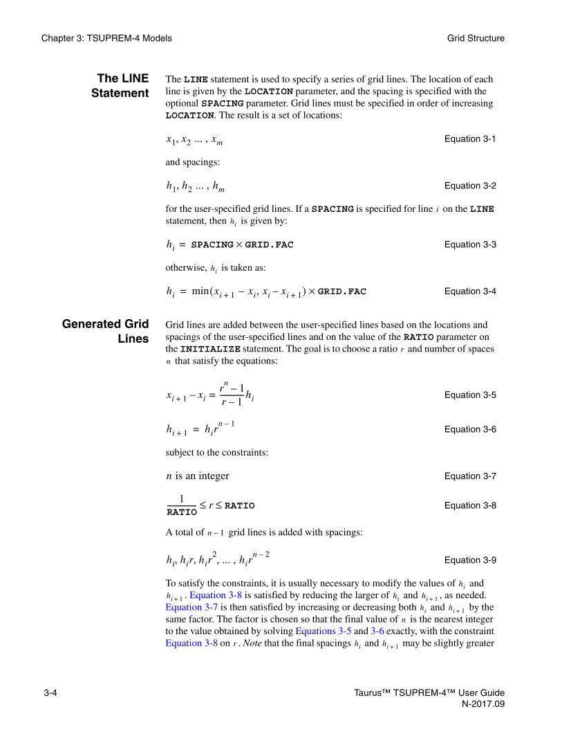
Chapter 3: TSUPREM-4 Models Grid Structure

The LINEStatement

The LINE statement is used to specify a series of grid lines. The location of each line is given by the LOCATION parameter, and the spacing is specified with the optional SPACING parameter. Grid lines must be specified in order of increasing LOCATION. The result is a set of locations:

Equation 3-1

and spacings:

Equation 3-2

for the user-specified grid lines. If a SPACING is specified for line on the LINE statement, then is given by:

Equation 3-3

otherwise, is taken as:

Equation 3-4

Generated GridLines

Grid lines are added between the user-specified lines based on the locations and spacings of the user-specified lines and on the value of the RATIO parameter on the INITIALIZE statement. The goal is to choose a ratio and number of spaces

that satisfy the equations:

Equation 3-5

Equation 3-6

subject to the constraints:

Equation 3-7

Equation 3-8

A total of grid lines is added with spacings:

Equation 3-9

To satisfy the constraints, it is usually necessary to modify the values of and . Equation 3-8 is satisfied by reducing the larger of and , as needed.

Equation 3-7 is then satisfied by increasing or decreasing both and by the same factor. The factor is chosen so that the final value of is the nearest integer to the value obtained by solving Equations 3-5 and 3-6 exactly, with the constraint Equation 3-8 on . Note that the final spacings and may be slightly greater

x1 x2 ... , xm,

h1 h2 ... , hm,

i

hi

hi SPACING= GRID.FAC×

hi

hi min xi 1+ xi, – xi xi 1+–( ) GRID.FAC×=

r

n

xi 1+ xir

n1–

r 1–-------------hi=–

hi 1+ hirn 1–

=

n is an integer

1RATIO---------------- r RATIO≤ ≤

n 1–

hi hir hir2

... , hirn 2–,,,

hi

hi 1+ hi hi 1+

hi hi 1+

n

r hi hi 1+

3-4 Taurus™ TSUPREM-4™ User GuideN-2017.09

Grid Structure Chapter 3: TSUPREM-4 Models

than their user-specified values, and the ratio may be slightly larger than RATIO or smaller than to satisfy the constraint that be an integer.

Two special cases should be noted: If and are both greater than or equal to the distance , then no grid lines are added between and ; and if and are equal, then uniformly spaced lines are added.

The and grids are generated independently, using the same algorithms.

Eliminating GridLines

The ELIMINATE statement (see Chapter 4, ELIMINATE, p. 4-58) can be used to thin out the grid in user-specified portions of the structure. The user specifies a rectangular subregion of the structure and whether vertical grid lines (COLUMNS) or horizontal grid lines (ROWS) are to be eliminated. The program then removes every other grid line in the specified direction within the specified region. Each additional ELIMINATE statement that specifies the region removes half of the remaining grid lines.

In some instances, it is not possible to eliminate grid lines when the specified region overlaps the region specified on a previous ELIMINATE statement. In these cases, a warning is printed and the elimination is not performed. The ELIMINATE statement is guaranteed to work when the specified region is the same as, totally included in, or totally separate from the regions specified on previous ELIMINATE statements.

The ELIMINATE statement is used during initialization to create a structure. It cannot be used to remove grid lines after initialization. The only way to remove grid lines after structure initialization is with STRUCTURE UNREFINE.

Automatic Grid Generation

If no LINE X statements are specified, grid lines in the x direction are generated automatically. Similarly, if no LINE Y statements are specified, the vertical grid is generated automatically. Automatic grid generation in either direction can be combined with manual grid generation in the other direction.

Automatic grid generation is controlled by parameters on the MESH statement and by the WIDTH and DX parameters on the INITIALIZE statement. Automatic grid generation in the x direction also depends on the location of mask edges obtained from mask information read with the MASK statement.

Automatic grid generation is intended for applications in which fine manual control over the grid is not needed. It is especially useful when mask information from the Taurus Layout—IC Layout Interface is available.

Note:Specifications for automatic grid generation can be put in the s4init file, allowing advanced users of TSUPREM-4 to set process-specific defaults for use by less experienced users.

r

1 RATIO⁄ n

hi hi 1+

xi 1+ xi– xi xi 1+ hi

hi 1+

x y

Taurus™ TSUPREM-4™ User Guide 3-5N-2017.09

Chapter 3: TSUPREM-4 Models Grid Structure

Automatic GridGeneration in the

X-Direction

A grid in the x direction (that is, a set of vertical grid lines) is generated automatically if an INITIALIZE statement without an IN.FILE is processed and no LINE X statements have been specified since the last INITIALIZE statement.

Placement of grid lines in the x direction is controlled by the DX.MIN, DX.MAX, and DX.RATIO parameters on the MESH statement and the WIDTH and DX parameters on the INITIALIZE statement. Automatic elimination of vertical grid lines is controlled by the LY.SURF and LY.ACTIV parameters on the MESH statement.

X Grid From WIDTHParameter

The WIDTH parameter on the INITIALIZE statement specifies the width of the device. The grid spacing in the x direction is specified by the DX parameter on the INITIALIZE statement or by DX.MAX on the MASK statement if DX is not specified.

X Grid From MASKStatement

If the WIDTH parameter is not specified, but a MASK statement has been used to read mask information, the locations of mask edges are used to guide generation of the grid. A line is placed at each mask edge, with spacing given by:

Equation 3-10

To either side of the mask edge, the grid spacing increases by a factor of DX.RATIO until a spacing of:

Equation 3-11

is reached, or until a point halfway between two mask edges is reached. A spacing of is used far from mask edges.

If the GRID parameter is used on the MASK statement, only edges on the specified mask levels are used for grid generation. If the G.EXTENT parameter is used, the spacing is used for the specified distance under the mask line before increasing towards .

Column Elimination If no ELIMINATE COLUMNS statements are specified, a default set of eliminate operations is performed on the vertical grid lines. One elimination is done between:

Equation 3-12

and the bottom of the structure. Eight eliminations are done between LY.ACTIV and the bottom of the structure. These eliminations are intended to remove all but two grid lines below LY.ACTIV.

If the WIDTH parameter is not specified and if no mask information has been read with a MASK statement, vertical grid lines are placed at x=0 and x=1 micron producing a grid for 1-D simulations.

hmin DX.MIN GRID.FAC×=

hmax DX.MAX GRID.FAC×=

hmax

hminhmax

y12--- LY.SURF LY.ACTIV+( )=

3-6 Taurus™ TSUPREM-4™ User GuideN-2017.09

Grid Structure Chapter 3: TSUPREM-4 Models

Automatic GridGeneration in the

Y-Direction

A grid in the y direction (that is, a set of horizontal grid lines) is generated automatically if an INITIALIZE statement without an IN.FILE is processed and if no LINE Y statements have been specified since the last INITIALIZE statement.

Automatic grid generation in the y direction is controlled by the LY.SURF, DY.SURF, LY.ACTIV, DY.ACTIV, LY.BOT, DY.BOT, and DY.RATIO parameters on the MESH statement.

For grid generation, the structure is divided into three regions.

• The surface region extends from y=0 down to LY.SURF, and has grid spacing . The surface region has the finest grid spacing. It

normally contains shallow implants and the channels of MOS transistors.

• The active region extends from LY.SURF down to LY.ACTIV and has a grid spacing that varies smoothly from to

. The active region extends to below the deepest junctions in the structure.

• The substrate region extends from LY.ACTIV to LY.BOT and has a grid spacing that starts at . It increases by factors of DY.RATIO until it reaches a spacing of . The substrate region is very deep, but has few vertical grid lines. It provides for accurate modeling of point defect recombination.

Note:The default values for the automatic grid generation parameters are typical of those required for simulating small-geometry MOS processes. Especially when using bipolar or power processes, you are encouraged to customize the default values for your needs.

Changes to the Mesh During Processing

The initial grid applies to the structure, not to the space containing the structure. Thus, processing steps that change the device structure must necessarily change the mesh structure as well. The processing steps that change the grid are deposition, epitaxy, etching, photoresist development, oxidation, and silicidation. In addition, if adaptive gridding is enabled, the grid may be modified during ion implantation and diffusion. The structure can also be truncated, reflected, or extended using the STRUCTURE statement.

DEPOSITION andEPITAXY

The DEPOSITION and EPITAXY statements deposit a conformal layer on the exposed surface of the structure (see Chapter 4, DEPOSITION, p. 4-101 and Chapter 4, EPITAXY, p. 4-142). The grid distribution normal to the exposed surface is controlled by four parameters:

• Layer thickness (THICKNES)

• Nominal grid spacing (DY)

DY.SURF GRID.FAC×

DY.USRF GRID.FAC×DY.ACTIV GRID.FAC×

DY.ACTIV GRID.FAC×DY.BOT GRID.FAC×

Taurus™ TSUPREM-4™ User Guide 3-7N-2017.09

Chapter 3: TSUPREM-4 Models Grid Structure

• Location of the nominal grid spacing relative to the top surface of the layer (YDY)

• Number of grid spaces in the layer (SPACES)

The thickness must always be specified. Effects produced by various combinations of parameters are as follows:

• If none of the other parameters is specified, a single grid space is placed in the layer.

• If SPACES or DY (but not both) is specified, a uniform grid spacing of THICKNES/SPACES or DY (multiplied by GRID.FAC) is used.

• If both SPACES and DY are specified, a nonuniform grid spacing is used, with a spacing of at a depth YDY below the surface and spacing that increases or decreases by a constant ratio for a total of

grid spaces. The grid spacing varies linearly from the value at YDY to the top and bottom of the layer, increasing or decreasing at the same rate on either side of YDY to produce the required number of grid spaces. Not all combinations of SPACES, DY, and YDY will produce a valid grid; in particular, the average grid spacing can never be less than half of DY.

Normally, the grid spacing parallel to the exposed surface is the same as the spacing along the original surface. However, when the grid spacing perpendicular to the surface is large compared to the parallel spacing, the parallel spacing is increased to avoid grid elements with low ratios of width to height. By default the width/height ratio is constrained to be at least 0.5, but this value can be changed with the AR.MIN parameter on the DEPOSITION or EPITAXY statements. Exposed corners on the original surface produce arcs at the surface of the deposited layer. These arcs are approximated by straight segments of length

or smaller.

StructureExtension

The STRUCTURE statement with the EXTEND parameter works similarly to deposition, except that grid is added horizontally to one edge of the structure; the parameters WIDTH, DX, and XDX are used in place of THICKNES, DY, and YDY. Note that XDX in this case is the absolute x coordinate at which the grid spacing specified by DX applies.

ETCH andDEVELOP

The ETCH and DEVELOP statements remove a specified portion of the structure. The grid is modified in two steps:

1. Nodes are added along the etch boundary. Nodes are placed at points where the etch boundary intersects the boundary of the material to be removed. Within the material being removed, the spacing of the added nodes is set to the smaller of the grid spacing of the points defining the etch boundary and the grid spacing in the material being removed.

2. Mesh elements inside the etch boundary are removed.

DY GRID.FAC×

SPACES GRID.FAC⁄

ARC.SPAC GRID.FAC×

3-8 Taurus™ TSUPREM-4™ User GuideN-2017.09

Grid Structure Chapter 3: TSUPREM-4 Models

Oxidation andSilicidation

The moving silicon/oxide interface and the material expansion produced during oxidation require continuous modifications to the simulation mesh. Three kinds of grid manipulation are required:

• Removal of nodes in consumed layers

• Addition of nodes in a growing layer (for example, during oxidation)

• Removal or rearrangement of nodes in regions where oxide is deforming

The following descriptions are in terms of oxidation, but apply equally to silicidation and other reactions. The only difference is that DY.DEFAU is used for the growing material instead of DY.OXIDE and GRID.OXI. This difference has no effect for any processes other than oxidation.

Removal of Nodes inConsumed Silicon

As oxidation occurs, the silicon/oxide interface advances into the silicon, while the growing oxide expands away from the silicon. Nodes (both silicon and oxide) on the interface move with the interface; nodes in the silicon interior remain fixed, while nodes in the oxide move with the oxide flow. As a consequence, interface nodes are continuously moving towards silicon nodes, which must be removed to allow the interface to advance.

Addition of Nodes ina Growing Layer

On the oxide side of the interface, the triangular mesh elements are expanding. To maintain solution accuracy in the oxide (for example, calculating the diffusion of oxidant in the oxide), it is necessary to add nodes to the oxide. The addition of nodes to the oxide is controlled by the DY.OXIDE, DY.EXACT, DY.LOCAL,and GRID.OXI parameters on the METHOD statement. (See Chapter 4, METHOD, p. 4-210.)

Precise grid spacing is obtained by adding new nodes in a growing layer at the distance specified by from an existing node in the layer. Because only one node can be added at each point on an interface during a simulation time step, the size of the time steps may need to be reduced to achieve the desired spacing. This reduction in the time step can be disabled by specifying ^DY.EXACT on the METHOD statement. By default, DY.EXACT is set to allow cutting of the time steps to control the grid spacing. The algorithm will not allow grid points to be added at spacings less than 1Å, and control of the spacing may not be precise for spacings less than 2Å.

The grid control algorithms and parameters apply to the entire structure. To avoid adding very fine grid in field regions when growing gate oxides, an option has been added to allow the grid spacing to vary with the oxide growth rate. When DY.LOCAL is specified on the METHOD statement, the grid spacing to be used at each point in the growing oxide is:

Equation 3-13

where is the growth rate at a point in the structure and is the maximum growth rate at all interfaces of the same type in the structure. (DY.DEFAU is used

DY.OXIDE GRID.FAC×

hvmax

v----------DY.OXIDE GRID.FAC×=

v vmax

Taurus™ TSUPREM-4™ User Guide 3-9N-2017.09

Chapter 3: TSUPREM-4 Models Grid Structure

instead of DY.OXIDE for reactions other than oxidation.) DY.LOCAL is set true by default.

If DY.OXIDE is zero, an extra node is added when the spacing in the oxide is approximately equal to the spacing in the silicon multiplied by the value of GRID.OXI. For (the silicon to silicon/dioxide volumetric expansion ratio) you might expect the number of nodes added to the oxide to equal the number of nodes removed from the silicon. Actually, more nodes are added to the oxide, because the apparent spacing of nodes in the silicon is reduced by the movement of the interface.The DY.OXIDE parameter is the preferred means of controlling grid spacing in the oxide. The GRID.OXI parameter is considered obsolete, and is retained only for compatibility with older versions of the program.

Nodes in RegionsWhere Oxide

Deforms

The flow of oxide may not be uniform when masking layers are present. At the edge of a nitride layer, for example, two corners of a triangular mesh element may be constrained by the presence of the nitride, while the third is being carried by the flow of oxide out from under the mask. In such situations, mesh triangles can become severely distorted, and could prevent further oxidation unless appropriate remedies are applied, such as flipping triangles and removing nodes or triangles in congested portions of the mesh. (In flipping triangles, the line common to two adjacent triangles is removed to form a quadrilateral, then a line is added to divide the quadrilateral into two triangles using the opposite two corners.)

In some cases, it may be necessary to eliminate a very thin triangle of one material that protrudes into another material. To avoid creating a hole in the structure, the material type of the triangle is changed to that of the surrounding structure.

Numerical Integrity After any modification to the mesh, a check is made for triangles that might lead to numerical difficulties (that is, loss of accuracy or poor convergence). Where possible, these triangles are eliminated by adjusting the triangularization or by adding nodes. Where such adjustment is not possible or would lead to large numerical errors, the discretization of the triangle is modified to avoid numerical instability.

Adaptive Gridding

To reduce the effort required to set up an initial grid and to improve simulation accuracy, TSUPREM-4 can perform adaptive mesh refinement during ion implantation, diffusion, and oxidation. It can perform adaptive mesh unrefinement during diffusion and oxidation.

Refinement Adaptive mesh refinement in TSUPREM-4 consists of splitting an edge of a triangle by adding a node at its midpoint if the estimated error at the midpoint is greater than the user-specified limit:

Equation 3-14

GRID.OXI 2.2=

ε REL.ADAP ERR.FAC C ABS.ADAP+××>

3-10 Taurus™ TSUPREM-4™ User GuideN-2017.09

Grid Structure Chapter 3: TSUPREM-4 Models

where REL.ADAP, ABS.ADAP, and ERR.FAC are parameters on the METHOD statement and is the value of a solution variable.

For adaptive gridding during ion implantation (with the analytical models):

• is the concentration of the impurity being implanted.

• is calculated directly from the ion implantation model.

No mesh refinement takes place during implants with the Monte Carlo (MC) model.

For adaptive gridding during diffusion:

• The calculation is done for each mobile impurity species, using values of based on estimates of the curvature of the impurity profile.

For adaptive gridding during oxidation:

• The calculation is done for the oxidizing species, using values of based on estimates of the curvature of the profile of the oxidant.

Separate values of REL.ADAP and ABS.ADAP are specified for each solution value in each material. ERR.FAC is a single value that scales the relative errors specified by REL.ADAP. The minimum grid spacing produced during adaptive refinement is specified for each solution value and material by the MIN.SPAC parameter on the METHOD statement.

Unrefinement Adaptive mesh unrefinement in TSUPREM-4 consists of removing mesh points that are not required to maintain the accuracy of the solution. The criterion for point removal is:

Equation 3-15

where UNREFINE is a parameter on the METHOD statement. Unrefinement is done twice in each diffusion step, about one quarter and three quarters of the way through the step. The maximum grid spacing produced by unrefinement is specified for each material by the MIN.SPAC parameter on the METHOD statement.

You can also request mesh unrefinement with the UNREFINE parameter on the STRUCTURE statement. The REPEAT parameter specifies the maximum number of unrefinement passes. Normally unrefinement does not remove points in the undoped (or background doped) substrate, but if ROWS or COLUMNS is specified on the STRUCTURE statement, these points can be removed. This can be useful in preparing a structure for device simulation. The unrefinement can be limited to a portion of the structure with the X.MIN, X.MAX, Y.MIN, and Y.MAX parameters.

C

C

ε

ε

ε

ε UNREFINE REL.ADAP ERR.FAC C ABS.ADAP+××( )×<

Taurus™ TSUPREM-4™ User Guide 3-11N-2017.09

Chapter 3: TSUPREM-4 Models Grid Structure

AdaptiveGridding for

Damage

The interstitial distribution is necessarily abrupt near amorphous and crystalline boundary after regrowth because the boundary location is determined by comparing implant damage concentration to the MAX.DAM parameter value, and then the interstitial concentration is reset to the equilibrium value in the regrowth region. Thus, the interstitial dose is sensitive to the mesh density near the boundary region. The adaptive gridding method based on the phase transition between amorphous and crystalline regions makes denser mesh near the boundary so that it increases simulation accuracy. Unlike the adaptive gridding of other solutions which uses the absolute and relative errors based on the solution values, the adaptive gridding for damage solution is performed on the transformed profile of damage:

Equation 3-16

Usage The IMP.ADAP parameter on the METHOD statement enables or disables adaptive gridding during ion implantation. The DIF.ADAP parameter enables or disables adaptive gridding (both refinement and unrefinement) during diffusion. The OX.ADAP parameter enables or disables adaptive gridding in oxide based on oxidant concentration. DAM.ADAP parameter enables or disables adaptive gridding in the region near amorphous and crystalline boundary. Refinement is disabled for impurity/material combinations for which REL.ADAP is zero. No unrefinement will occur in materials for which MIN.SPAC is zero, and no unrefinement will occur if UNREFINE is zero.

Note:IMP.ADAP and DAM.ADAP are applicable for analytic implants for regrid prior to a Monte Carlo implant.

Adaptive gridding reduces the impact of the initial grid on the speed and accuracy of the simulation but does not eliminate it entirely. Meshes that rely heavily on adaptive gridding tend to be less regular than manually specified meshes of similar density. Results using these irregular meshes may appear less accurate because of the irregular variation of the numerical error from point to point. Regular, manually generated meshes may be preferable when precise comparison of similar solutions is required.

Even with adaptive gridding, you must verify that the following requirements are met to ensure accurate simulations:

• The initial grid spacing in layers that receive implants must be smaller than the standard deviation of the implanted profile.

• When an epitaxial layer is grown on a substrate with a high surface impurity concentration, the first grid space in the epi layer must be small compared to the expected depth of out-diffusion into the epi layer.

There may be cases where you want to modify or disable adaptive gridding:

• Adaptive refinement during diffusion following a MC implant may cause a large number of nodes to be added in response to statistical variations in the

s 1 DAM.GRAD ln D0 MAX.DAMA⁄( )×[ ]tanh+=

3-12 Taurus™ TSUPREM-4™ User GuideN-2017.09

Grid Structure Chapter 3: TSUPREM-4 Models

implanted profile. It is often a good idea to disable DIF.ADAP during the first few minutes of diffusion following a MC implant.

• When oxidizing through a poly layer you may want to disable OX.ADAPT between the time when the oxidation first breaks through the poly and the time when the poly layer has been consumed across its entire width. This avoids adding unnecessary extra nodes in the pad oxide under the poly.

• In situations where less accuracy is needed, you may want to set ERR.FAC to a value greater than 1. Similarly, where more accuracy is needed you may want to use a value less than 1.

• For large structures that undergo long high-temperature diffusion cycles, you may want to be more aggressive in removing unneeded mesh points. It is usually safe to use values of UNREFINE as high as 1.0.

• There may be cases where unrefinement is removing mesh points you will soon be needing. (For example, nodes near the surface may be removed prior to an implant that needs them.) In this case you can disable unrefinement by setting UNREFINE to 0 until the points are used.

• You may want to reduce the value of MAX.SPAC in silicon for small geometry devices and increase the value for power devices.

1-D Simulation of Simple Structures

In many simulations, the geometry and doping vary in the y direction only. Such structures are represented internally as 1-D structures, with considerable savings in simulation time and memory requirements.

1-D structures are automatically converted to 2-D structures whenever an etch or expose step destroys the uniformity of the structure in the x direction. 1-D structures are also converted to two dimensions for display (using the PLOT.2D statement) or saving to a file. Such conversions are temporary, and 1-D simulation resumes after plotting or saving.

All saved structures are stored as 2-D structures; structures that are uniform in the x direction are converted to 1-D structures when they are read from a file. Full 2-D simulation of 1-D structures can be forced by specifying ^FAST on the MESH statement.

Initial Impurity Concentration

The initial impurity concentration in a structure can be specified directly or by specifying the resistivity of the material. In either case, one of two styles can be used:

• In the old-style specification, ANTIMONY, ARSENIC, BORON, and PHOSPHOR parameters are used to set the impurity concentration or resistivity of antimony, arsenic, boron, and phosphorus, respectively; CONCENTR or RESISTIV is used to determine whether the concentration or resistivity is specified.

Taurus™ TSUPREM-4™ User Guide 3-13N-2017.09

Chapter 3: TSUPREM-4 Models Diffusion

• In the new-style specification, impurity is specified by name with the IMPURITY parameter and the concentration or resistivity is specified with the I.CONC or I.RESIST parameters.

The old-style and new-style specifications can be mixed when specifying impurity concentrations directly, that is, the IMPURITY and I.CONC parameters can be used on the same statement with the ANTIMONY, ARSENIC, BORON, and PHOSPHOR parameters. Only one impurity can be specified when RESISTIV or I.RESIST is specified.

When the resistivity is specified, the concentration is given by:

Equation 3-17

where and are the electron and hole mobilities, respectively, and is the resistivity. The carrier mobilities are contained in three internal tables—one for hole mobility in p-type silicon, one for electron mobility in arsenic- and antimony-doped silicon, and one for electron mobility in silicon doped with other donor impurities. The tables are from Masetti, et al. Reference [2].

Note:The mobility tables used for determining the initial concentration are not the same as those used for calculating sheet resistance with the ELECTRICAL statement. Thus, the extracted sheet resistance is not identical to the specified resistivity of the starting material.

The same calculation is used for all materials, even though it is only meaningful for silicon and polysilicon; a warning is printed if the resistivity is specified for other materials.

Specification of the initial impurity concentration is the same for the INITIALIZE, DEPOSITION, and EPITAXY statements.

DiffusionThe most fundamental process simulated by TSUPREM-4 is diffusion, which, when performed in an oxidizing ambient or in the presence of an appropriate metal, also produces oxidation or silicidation. In addition to simulating the diffusion of the dopant atoms, TSUPREM-4 models the diffusion of point defects (that is, self-interstitials and vacancies) and, in some cases, an oxidizing species (assumed to be O2 or H2O). For silicidation, diffusion of metal and/or silicon atoms through silicide is modeled. The models used by the DIFFUSION statement are described in the following sections.

C

1qμnρ------------ donor impurity

1qμpρ------------ acceptor impurity

=

μn μp ρ

3-14 Taurus™ TSUPREM-4™ User GuideN-2017.09

Diffusion Chapter 3: TSUPREM-4 Models

DIFFUSION Statement

The DIFFUSION statement (see Chapter 4, DIFFUSION, p. 4-136) is used to model the diffusion of impurities under oxidizing and nonoxidizing conditions. The duration of the diffusion step (in minutes) is specified with the TIME parameter.

Temperature The initial temperature of the step (in °C) is given by the TEMPERAT parameter. Linear variation of the temperature over the step can be specified with the T.RATE or T.FINAL parameters. If T.RATE is specified, the temperature varies as:

Equation 3-18

where is the time since the start of the step and is the diffusion temperature (in °C) at time . If T.FINAL is specified, the temperature varies as:

Equation 3-19

If neither T.RATE nor T.FINAL is specified, the temperature is constant. The physical coefficients that depend on temperature are presumed to be valid in the range 800 to 1250×°C, but temperatures outside this range are allowed.

Ambient GasPressure

The pressure of the ambient gas during the step can vary linearly with time, and is specified with the PRESSURE parameter and either the P.RATE or P.FINAL parameter. The PRESSURE parameter specifies the initial pressure. If neither P.RATE nor P.FINAL is specified, the pressure is constant. If P.RATE is specified, the pressure varies as:

Equation 3-20

where is the time since the start of the step and is the pressure at time . If P.FINAL is specified, the pressure varies as:

Equation 3-21

These values must be chosen to yield positive, nonzero pressures throughout the step.

Ambient GasCharacteristics

The characteristics of the ambient gas can be specified in one of two ways:

• Specify a previously defined ambient with one of the parameters DRYO2, WETO2, STEAM, INERT, AMB.1, AMB.2, AMB.3, AMB.4, or AMB.5.

• Define the ambient gas directly by specifying the flows of the oxidizing and nonoxidizing species with the parameters F.O2, F.H2O, F.H2, F.N2, and F.HCL or HCL.

Tc TEMPERAT T.RATE t×+=

t Tc

t

Tc TEMPERATT.FINAL TEMPERAT–( )

TIME------------------------------------------------------------t+=

P PRESSURE P.RATE t×+=

t P t

P PRESSUREP.FINAL PRESSURE–( )

TIME------------------------------------------------------------t+=

Taurus™ TSUPREM-4™ User Guide 3-15N-2017.09

Chapter 3: TSUPREM-4 Models Diffusion

Ambients andOxidation of

Materials

The characteristics of defined ambients and the physical coefficients describing the oxidation of materials are specified with the AMBIENT statement(see Chapter 4, AMBIENT, p. 4-236). The flows of the oxidizing and nonoxidizing species associated with the ambient are specified with the F.O2, F.H2O, F.H2, F.N2, and F.HCL parameters. The default gas pressure can be specified for the ambient with the PRESSURE parameter, and the default chlorine percentage can be specified with HCL.

If flows of both O2 and H2 are present in the ambient, these gases are assumed to undergo a complete pyrogenic reaction to form H2O as given by:

Equation 3-22

The final flows of O2, H2, and H2O after the pyrogenic reaction are given by:

Equation 3-23

Equation 3-24

Equation 3-25

The partial pressures of the oxidizing species are given by:

Equation 3-26

Equation 3-27

If the resulting ambient contains both O2 and H2, the oxidation rate is based on the partial pressure of H2O.

Default Ambients The following default ambients are defined:

• DRYO2: The dry oxygen ambient contains 100% O2.

• WETO2: The wet oxygen ambient contains 92% H2O and 8% N2. This reflects evidence that wet O2 (oxygen bubbled through H2O at 95°C) is equivalent to pyrogenic steam with O2 and H2 flow rates of 1.175 and 2.0 liters/minute, respectively Reference [3]. (The actual ambient contains 8% O2, but because TSUPREM-4 cannot model simultaneous oxidation by H2O and O2, nitrogen is substituted for the oxygen in the simulation.)

• STEAM: The steam ambient contains 100% H2O. This represents formation of H2O by a complete pyrogenic reaction of O2 and H2, without excess O2 or H2.

• INERT: The inert ambient contains 100% N2 (or other inert gasses).

The default PRESSURE for each of these ambients is 1 atmosphere.

H212---O2 H2O→+

FO2 F.O2 min F.O2,F.H22

------------- –=

FH2 F.H2 min 2 F.O2,F.H2×( )–=

FH2O F.H2O min 2 F.O2,F.H2×( )+=

PO2

FO2

FO2 FH2O FH2 F.N2 F.HCL+ + + +-----------------------------------------------------------------------------------P=

H20

FH2O

FO2 FH2O FH2 F.N2 F.HCL+ + + +-----------------------------------------------------------------------------------P=

3-16 Taurus™ TSUPREM-4™ User GuideN-2017.09

Diffusion Chapter 3: TSUPREM-4 Models

Chlorine The inclusion of chlorine in the ambient is specified with either the HCL or F.HCL parameter. These parameters are related by:

Equation 3-28

where , , and are the final flows of O2, H2, and H2O, respectively, after the pyrogenic reaction of O2 and H2 to form H2O. The chlorine percentage is defined as 100 times the mole fraction of atomic chlorine relative to the total ambient gas.

Example For example, in dry oxygen 1% chlorine represents the presence of one chlorine atom for every 99 O2 molecules. Either HCL or F.HCL can be used when defining an ambient on the AMBIENT or DIFFUSION statement. If HCL is specified along with a predefined ambient on the DIFFUSION statement, the specified chlorine percentage is used instead of the percentage or flow rate defined for the ambient.

Coefficient Tables The effects of chlorine in the ambient gas on the oxidation rate of silicon are represented by tables of coefficients that modify the linear oxidation rate. The tables are specified with the AMBIENT statement. (See Chapter 4, AMBIENT, p. 4-236.) The tables are 2D with the rows representing chlorine percentages and the columns representing diffusion temperatures. Linear interpolation is used to obtain values for temperatures or percentages between the values in the table. For temperatures or percentages outside the range of values present in the tables, the values in the first or last rows or columns, as appropriate, are used. (See Analytical Oxidation Models, p. 3-101 for the use of the coefficients in these tables.)

ChemicalPredeposition

A chemical predeposition step can be modeled with the DIFFUSION statement by specifying the concentrations of one or more impurities in the ambient gas. The impurity concentrations are specified explicitly with the parameters ANTIMONY, ARSENIC, BORON, and PHOSPHOR or with the IMPURITY and I.CONC parameters. Impurities can also be included in a thermal oxidation step, but the resulting oxide is always modeled as a high-quality thermal oxide; the effects of high impurity concentrations on the oxide characteristics are not simulated.

Solution ofDiffusion

Equations

The diffusion equations are nonlinear because of the dependence of the diffusion coefficients and electric field on the impurity, point defect, and carrier concentrations. These dependencies also couple the equations for multiple impurities and point defects. An accurate solution to this coupled nonlinear system is obtained by dividing the total diffusion time specified by the TIME parameter into a series of smaller time steps represented by . The initial time step is set by the INIT.TIM parameter on the METHOD statement (see Chapter 4, METHOD, p. 4-210). For each time step thereafter, the value of is made as large as possible while holding the estimated error in the solution to acceptably small values. The time step is chosen to satisfy Reference [4].

HCL 100 F.HCL

FO2 FH2O FH2 F.N2 F.HCL+ + + +-----------------------------------------------------------------------------------=

FO2 FH2 FH20

Δt

Δt

Δt

Taurus™ TSUPREM-4™ User Guide 3-17N-2017.09

Chapter 3: TSUPREM-4 Models Diffusion

Equation 3-29

where:

• is the number of nodes in the structure.

• is the number of diffusing species (impurities and point defects) at each node.

• is the concentration of species at node .

• is the estimated error in .

• REL.ERR and ABS.ERR are the relative and absolute error for each species, specified with the METHOD statement.

The time step may be also be reduced during oxidation to avoid numerical difficulties or to prevent mesh tangling.

Diffusion of Impurities

This section describes the equations that model the diffusion of dopant atoms in the device structure. Diffusion of dopants is simulated in all materials.

The diffusion equation solved for each impurity present in the structure is:

Equation 3-30

where:

• is the chemical impurity concentration.

• is the divergence operator.

Impurity Fluxes The impurity fluxes in the interior of a material region are given by:

Equation 3-31

Equation 3-32

1n---

ΔCij

REL.ERRj Cij ABS.ERRj+⋅-------------------------------------------------------------------

j 1=

m

2

i 1=

n

1≤

n

m

Cij j i

ΔCij Cij

∂C∂t------- ∇ Jm Jn+( )⋅–=

C

∇ .

Jm Dm ∇ CmMM′------

zs CmMM′------

qEkT-------– Cm

MM′------

VFSUBkT

------------------∇p +–=

Jn Dn ∇ CmNN′-----

zs CmNN′-----

qEkT-------– Cm

NN′-----

VFSUBkT

------------------∇p +–=

3-18 Taurus™ TSUPREM-4™ User GuideN-2017.09

Diffusion Chapter 3: TSUPREM-4 Models

where:

• and are the flux and diffusivity of impurities diffusing with (or as) interstitials.

• and are the flux and diffusivity of impurities diffusing with vacancies.

• is the charge of the ionized impurity (+1 for donors and –1 for acceptors).

• is the electronic charge.

• is Boltzmann’s constant.

• is the absolute temperature.

• is the mobile impurity concentration.

• is the gradient operator.

• and model the enhancement (or retardation) of diffusion due to nonequilibrium point defect concentrations.

• is the hydrostatic pressure. VFSUB is the parameter associated with the pressure-dependent substitutional atom formation energy. This is only applicable when the boolean parameters ST.EFORM or ST.ALPHA in the METHOD statement are turned on. See Pressure Dependence of Migration Energy, p. 3-23.

Mobile Impuritiesand Ion Pairing

TSUPREM-4 includes a model for the pairing of positively and negatively charged dopant ions, see References [5], [ 6 ], and [ 7 ]. This model reduces the concentration of mobile dopant atoms according to:

Equation 3-33

Equation 3-34

where is the electrically active dopant concentration (see Activation of Impurities, p. 3-35), and and are the ion pairing factors for donors and acceptors, respectively. Ion pairing reduces the diffusivity of dopants where the concentration of dopants of the opposite type is large.

The ion pairing model assumes that positively charged donors can bind with negatively charged acceptors to form neutral pairs:

Equation 3-35

The forward reaction rate is proportional to the number of unpaired donor and acceptor ions, while the reverse reaction rate is proportional to the number of pairs. In equilibrium:

Equation 3-36

Jm Dm

Jn Dn

zs

q

k

T

Cm

∇

M M′⁄ N N′⁄

p

Cm

Cm Fpd Ca donors( )=

Cm Fpa Ca= acceptors( )

CaFpd Fpa

D+

A-

P→←+

Nd( Np ) Na Np–( ) ΩNp=–

Taurus™ TSUPREM-4™ User Guide 3-19N-2017.09

Chapter 3: TSUPREM-4 Models Diffusion

Where and are the total concentrations of electrically active donors and acceptors, respectively, is the concentration of ion pairs, and is a proportionality factor. Equation 3-36 can be solved for the number of ion pairs, giving:

Equation 3-37

The pairing factors are then given by:

Equation 3-38

Equation 3-39

The parameter is given by:

Equation 3-40

where IP.OMEGA is a parameter on the MATERIAL statement; the default value for silicon and polysilicon is 6.0 Reference [6]. The ion pairing model is enabled or disabled for each material by the ION.PAIR parameter on the MATERIAL statement; by default, it is enabled for silicon and polysilicon, but disabled for all other materials, including new user-defined materials.

The ion pairing model is significant because it allows the dependence of the impurity diffusivity to be modeled in both n-type and p-type materials. In particular, it may reduce the effective diffusivity of boron in n-type materials without affecting its diffusivity at high p-type concentrations.

Electric Field In insulator and conductor materials, the electric field vector is zero. In semiconductor materials, the electric field is given by:

Equation 3-41

where is the ratio of the electron concentration to the effective intrinsic carrier concentration, that is, . The distribution of the charge carriers can be extracted either by assuming local charge neutrality or by numerically solving the

Nd NaNp Ω

Np12--- Nd( Na Ω ) Nd( Na Ω )2

4Nd Na–+ +–+ +=

Fpd 1NpNd------–

= donors( )

Fpa 1NpNa------–

= acceptors( )

Ω

Ω IP.OMEGA ni=

E

E ∇ψ–=

kTq

------∇ηη

--------–=

ηn nie⁄

3-20 Taurus™ TSUPREM-4™ User GuideN-2017.09

Diffusion Chapter 3: TSUPREM-4 Models

Poisson equation. By default, local charge neutrality is assumed so that the electron concentration is written as:

Equation 3-42

where:

• and are the sums of the electrically active donor and acceptor impurity concentrations, respectively.

• is the effective intrinsic carrier concentration given by:

Equation 3-43

Equation 3-44

where EG.ADD, NI.0, NI.E, and NI.F are specified in the MATERIAL statement. EG.ADD can be specified with a number or an expression.

Presence of the electric field term produces couplings among the diffusion equations for the different impurities.

Note:Turning on the POISSON parameter in the METHOD statement specifies that the Poisson equation is to be solved instead of assuming local charge neutrality. The Poisson equation is solved only for silicon or polysilicon materials. However, in polycrystalline material, the electric field on grain boundary is always calculated by local charge neutrality regardless of the specification of solving the Poisson equation.

The electrically active and mobile impurity concentrations ( and , respectively) are assumed to be the same. The model for calculating these values is described in Activation of Impurities, p. 3-35.

nNd Na–

2------------------

Nd Na–

2------------------

2

nie2

++=

Nd Na

nie

nie niEG.ADD–

2kT----------------------- exp=

ni NI.0 exp NI.E–kT

---------------- TNI.F⋅=

Ca Cm

Taurus™ TSUPREM-4™ User Guide 3-21N-2017.09

Chapter 3: TSUPREM-4 Models Diffusion

Diffusivities It is assumed that impurities diffuse in semiconductor materials as dopant-defect pairs. The diffusion coefficients and are sums of the effective diffusivities of impurities due to pairing with defects in various charge states:

Equation 3-45

The components of diffusivity are given by:

Equation 3-46

Equation 3-47

where the parameters DIX.0, DIX.E, DIP.0, DIP.E, DIM.0, DIM.E, DIMM.0, DIMM.E, DVX.0, DVX.E, DVP.0, DVP.E, DVM.0, DVM.E, DVMM.0, and DVMM.E are specified in the ANTIMONY, ARSENIC, BORON, and PHOSPHORUS statements (see Chapter 4, PHOSPHORUS, p. 4-371).

Diffusivities for arbitrary charge states are given by:

Equation 3-48

where the parameters DIC.0, DIC.E, DVC.0, and DVC.E for the charge state are specified on the IMPURITY statement (see Chapter 4,

IMPURITY, p. 4-281).

PolysiliconEnhancement

The factor FGB is applied only for materials for which the polycrystalline model is disabled, and only if the value specified is nonzero. It compensates for the omission of the grain-boundary diffusion flux in polycrystalline materials when the polycrystalline diffusion models are not used.

Dm Dn

Dm Fstn Fstsm FGB⋅ ⋅ DI.FAC DI.F11 0

0 DI.F22Dmkη k–

k 6–=

6

⋅ ⋅⋅=

Dn Fstn Fstsn FGB⋅ ⋅ DV.FAC DV.F11 0

0 DV.F22Dnkη k–( )

k 6–=

6

⋅ ⋅⋅=

Dmk Fαm D0 mk, Dnk Fαn D0 nk,⋅=⋅=

D0 m0, DIX.0 exp DIX.E–kT

------------------- ⋅= D0 n0, DVX.0 exp DVX.E–

kT------------------- ⋅=

D0 m1, DIP.0 exp DIP.E–kT

------------------- ⋅= D0 n1, DVP.0 exp DVP.E–

kT------------------- ⋅=

D0 m 1–( ), DIM.0 exp DIM.E–kT

------------------- ⋅= D0 n 1–( ), DVM.0 exp DVM.E–

kT------------------- ⋅=

D0 m 2–( ), DIMM.0 exp DIMM.E–kT

----------------------- ⋅= D0 n 2–( ), DVMM.0 exp DVMM.E–

kT----------------------- ⋅=

D0 mk, DIC.0 exp DIC.E–kT

------------------- ⋅= D0 nk, DVC.0 exp DVC.E–

kT------------------- ⋅=

k C.STATE=

3-22 Taurus™ TSUPREM-4™ User GuideN-2017.09

Diffusion Chapter 3: TSUPREM-4 Models

User-DefinedIsotropic

Multiplication

The diffusivities can be multiplied by the parameters DI.FAC and DV.FAC in the IMPURITY statement. Parameters values can be numbers or formulas. This provides the method for users to define more complicated diffusivity models.

User-DefinedAnisotropic

Multiplication

Dopant diffusion in presence of anisotropic stress is not isotropic anymore. To provide the modeling capability for this type of anisotropic diffusion, the user-specified tensor expression can be taken. It describes the anisotropic diffusion path, which is given by the parameters DI.F11, DI.F22, DV.F11, and DV.F22 in the IMPURITY statement. Each parameter can be given by any formula expression.

PressureDependence of

Migration Energy

The pressure dependence of the migration energy of a dopant-defect pair or a substitutional atom is modeled by assuming that the migration energy depends linearly on the pressure and a activation volume, VMIPAIR for a dopant-interstitial pair and VMVPAIR for a dopant-vacancy pair. The factors Fstsm or Fstsn are applied only for diffusion in silicon materials for which the stress history is modeled, and the ST.DIFF model is enabled. The activating volumes, VMIPAIR and VMVPAIR, have a dimension of A3 and are specified in the IMPURITY statement. The parameters for setting stress history and stress dependent diffusion are specified in the METHOD statement.

Equation 3-49

Note:If you define VD, the value of VD is assigned to both VMIPAIR and VMVPAIR.

PressureDependence of

Formation Energy

The pressure dependence of the formation energy of a dopant-defect pair and a substitutional atom is modeled by assuming that the formation energy depends linearly on the pressure and a activation volume, VFIPAIR for a dopant-interstitial pair, VFVPAIR for a dopant-vacancy pair and VFSUB for a substitutional atom. The factors Fαm and Fαn are applied only for diffusion in silicon materials for which the stress history is modeled, and either the ST.EFORM model or the ST.ALPHA model is enabled. The activating volumes, VFIPAIR, VFVPAIR and VFSUB have a dimension of A3 and are specified in the IMPURITY statement. The parameters for setting stress history and stress dependent diffusion are specified in the METHOD statement.

Equation 3-50

p

Fstsm expp VMIPAIR⋅–

kT--------------------------------- , Fstsn exp

p VMVPAIR⋅–kT

--------------------------------- = =

p

Fαm expp VFIPAIR VFSUB–( )⋅–

kT------------------------------------------------------------- =

Fαn expp VFVPAIR VFSUB–( )⋅–

kT------------------------------------------------------------- =

Taurus™ TSUPREM-4™ User Guide 3-23N-2017.09

Chapter 3: TSUPREM-4 Models Diffusion

Note:If you define VALPHAM instead of VFIPAIR, the value of VFIPAIR is calculated by VALPHAM+VFSUB; similarly, VFVPAIR from VALPHAN+VFSUB.

Figure 3-1 Energy diagram for pressure-dependent migration/formation energy for interstitial and dopant-interstitial pair

Point Defect Enhancement

The definition of the point defect enhancement factors and depends on the NSTREAMS, PAIR.SAT, and PAIR.REC parameters specified on the METHOD statement. For NSTREAMS =1 (for example, if PD.FERMI is set on the METHOD statement) and in materials other than silicon, the point defect concentrations are assumed to be at their thermal equilibrium values so that:

PD.FERMI Model Equation 3-51

and Equations 3-30, 3-31, and 3-32 reduce to:

Equation 3-52

Em(I)ST. DIFFVD

Em(Ai)ST. DIFFVMIPAIR

Ef(Ai)ST. EFORMVFIPAIR

Ef(I)ST. EFORMVCEQUIL

Ef(As)ST. EFORMVFSUB

Eb(Ai)

E(Dm) E(αm)

M M'⁄ N N'⁄

MM′------

NN′----- 1= =

C∂t∂

------ ∇– Dm Dn+( ) ∇Cm zsCmqEkT-------– VFSUB Cm

∇pkT-------⋅+

–⋅=

3-24 Taurus™ TSUPREM-4™ User GuideN-2017.09

Diffusion Chapter 3: TSUPREM-4 Models

PD.TRANS andPD.FULL Models

For NSTREAMS =3 (for example, if PD.TRANS or PD.FULL is set on the METHOD statement), use the full equations for the enhancement factors:

Equation 3-53

Equation 3-54

and are the ratios of the dopant-defect pair concentrations to the substitutional dopant concentration under equilibrium conditions. They are used to define and :

Equation 3-55

Equation 3-56

The values of and are calculated from:

Equation 3-57

where:

Equation 3-58

Equation 3-59

MM′------

I

I*

----Km Kmv

I*

I----+

Km KmvV

V*

------+------------------------------

1 αmI

I*

----Km Kmv

I*

I----+

Km KmvV

V*

------+------------------------------

αnV

V*

------Kn Kni

V*

V------+

Kn KniI

I*

----+---------------------------

+ +

---------------------------------------------------------------------------------------------------------------=

NN′-----

V

V*

------Kn Kni

V*

V------+

Kn KniI

I*

----+---------------------------

1 αmI

I*

----Km Kmv

I*

I----+

Km KmvV

V*

------+------------------------------

αnV

V*

------Kn Kni

V*

V------+

Kn KniI

I*

----+---------------------------

+ +

---------------------------------------------------------------------------------------------------------------=

αm αn

M′ N′

M′ αmCm≡

N′ αnCm≡

αm αn

αm

Dmk

DMk----------η k–

k= and αn

Dnk

DNk---------η k–

k=

DMk DIPAIR.0 exp DIPAIR.EkT

--------------------------– ⋅=

DNk DVPAIR.0 exp DVPAIR.EkT

--------------------------– ⋅=

Taurus™ TSUPREM-4™ User Guide 3-25N-2017.09

Chapter 3: TSUPREM-4 Models Diffusion

and DIPAIR.0, DIPAIR.E, DVPAIR.0, and DVPAIR.E are parameters on the IMPURITY, ANTIMONY, ARSENIC, BORON, and PHOSPHORUS statements. Physically, and are the diffusivities of the (z+k)-charged dopant-defect pairs; they are expected to have values comparable to the diffusivities of interstitials and vacancies, respectively. The charge state (z+k)’s of the dopant-interstitial pairs and the dopant-vacancy pairs are specified with the parameters C.IPAIR and C.VPAIR, respectively. Instead, turing on the boolean parameters C.IP.ALL and C.VP.ALL assumes the diffusivities of dopant-interstitial pairs and dopant-vacancy pairs respectively to be independent of charge state.

Paired Fractionsof Dopant Atoms

The values of and vary with the Fermi level, but do not otherwise depend on the dopant or defect concentrations. Physically, they represent the fractions of dopant atoms that are coupled with interstitials and vacancies. The and terms prevent the pair concentrations from exceeding the total dopant concentrations when the concentrations of point defects are very high Reference [8]. These terms are calculated only if PAIR.SAT is true (set on the METHOD statement, directly or by specifying PD.FULL); otherwise, they are set to 0.

5-StreamDiffusion Model

Setting the parameter NSTREAMS to 5 or turning on the parameter PD.5STR specifies to solve the transient equations of both dopant-interstitial and dopant-vacancy pairs:

Equation 3-60

Equation 3-61

where and are the reaction rates for generation of dopant-interstitial and dopant-vacancy pairs, respectively;

Equation 3-62

Equation 3-63

and are the dopant-assisted recombination rates for interstitials and vacancies;

Equation 3-64

Equation 3-65

DMk DNk

αm αn

αm αn

t∂∂M ∇ Jm Gm Rm–( ) Gmv Rmv–( )– RDDCM–+⋅–=

t∂∂N ∇ Jn Gn Rn–( ) Gni Rni–( )– RDDCN–+⋅–=

Gm Rm– Gn Rn–

Gm Rm– Km SI

I*

---- M

αm-------–

=

Gn Rn– Kn SV

V*

------ N

αn------–

=

Gmv Rmv– Gni Rni–

Gmv Rmv– KmvMαm------- V

V*

------ S–

=

Gni Rni– KniNαn------ I

I*

---- S–

=

3-26 Taurus™ TSUPREM-4™ User GuideN-2017.09

Diffusion Chapter 3: TSUPREM-4 Models

and and are the reaction rate of dopant-interstitial and dopant-vacancy pairs, respectively, for dopant-defect clusters (see the details in the DDC.FULL model description):

Equation 3-66

Equation 3-67

The concentration S of substitutional atoms is calculated by;

Equation 3-68

The flux equations of dopant-interstitial pairs and dopant-vacancy pairs are given by:

Equation 3-69

Equation 3-70

Initialization ofPairs

The parameters IP.FRACA, VP.FRACA and S.FRACA in the IMPURITY statement determines the redistribution of the dopant-defect pairs and the substitutional atoms in the epitaxial regrowth region as follows;

Equation 3-71

Equation 3-72

BoundaryConditions for

Pairs

The flux of dopant-defect pairs at silicon boundary can be calculated by one of the following models;

• Surface recombination flux

• Segregation flux

Turning on PAIR.SEG in the METHOD statement applies the segregation flux of pairs instead of the surface recombination flux.

RDDCM RDDCN

RDDCM RDDC S M+, RDDC I M+, RDDC I n( ) M+,2RDDC M M+, RDDC C M+, RDDC V n 1+( ) M+,

RDDC XI2 V+,–

+ ++ + +

=

RDDCN RDDC S N+, RDDC V N+, RDDC V n( ) N+,2RDDC N N+, RDDC C N+, RDDC I n 1+( ) N+,

RDDC XV2 I+,–

+ ++ + +

=

S Cm M– N–=

Jm Dm ∇ Mαm------- zs

Mαm------- qE

kT-------–

Mαm------- VFSUB

kT------------------∇p +

⋅–=

Jn Dn ∇ Nαn------ zs

Nαn------ qE

kT-------–

Nαn------ VFSUB

kT------------------∇p +

⋅–=

M IP.FRACA

IP.FRACA VP.FRACA S.FRACA+ +---------------------------------------------------------------------------------------- Cm=

N VP.FRACA

IP.FRACA VP.FRACA S.FRACA+ +---------------------------------------------------------------------------------------- Cm=

Taurus™ TSUPREM-4™ User Guide 3-27N-2017.09

Chapter 3: TSUPREM-4 Models Diffusion

SurfaceRecombination of

Dopant-Defect Pairs

The surface recombination rates of pairs in the 5-stream diffusion model can be defined for the interface between two materials in the IMPURITY statement. The parameters KSIP.0 and KSIP.E define the prefactor and the activation energy for the surface recombination of dopant-interstitial pairs, respectively. Likewise, KSVP.0 and KSVP.E for dopant-vacancy pairs.

Equation 3-73

Equation 3-74

where:

Equation 3-75

Equation 3-76

and are defined as follows:

Equation 3-77

Equation 3-78

Pair SegregationModel

The segregation model for dopant-interstitial pairs is derived with the following reaction:

Equation 3-79

where is the concentration of (z+k)-charged dopant-interstitial pairs, is the concentration of dopants at the boundary of a neighbor material adjacent to silicon material, is the k-charged interstitial at silicon boundary which is generated by the dissociation of the dopant-interstitial pair. Likewise, for dopant-vacancy pairs,

Equation 3-80

For the 2-phase segregation model (Segregation of Impurities, p. 3-63):

Equation 3-81

Fm kms M∗ M–( )=

Fn kns N∗ N–( )=

M∗αm

1 αm αn+ +-----------------------------C=

N∗αn

1 αm αn+ +-----------------------------C=

kms kns

kms KSIP.0KSIP.E

kT---------------------–

exp⋅=

kns KSVP.0KSVP.E

kT---------------------–

exp⋅=

M z k+( ) qijn+ Cj I k( ) qjin+ +↔

M z k+( ) Cj

I k( )

N z k+( ) qijn+ Cj V k( ) qjin+ +↔

Fm SEG.IFRA hI

Ii0*

----- SEG.IPOW

Cjηqji M

αmI I*⁄

------------------ η

qij

m--------–

⋅=

3-28 Taurus™ TSUPREM-4™ User GuideN-2017.09

Diffusion Chapter 3: TSUPREM-4 Models

Equation 3-82

For the interface trap model (Interface Trap Model, p. 3-64):

Equation 3-83

Equation 3-84

Unlike the pair surface recombination model, the interstitial and vacancy concentrations and the dopant concentration at silicon boundaries are directly affected by Equation 3-79 and Equation 3-80. The generation flux of interstitial and vacancy at silicon boundary due to pair segregation is and , respectively. The segregation flux of total dopant concentration is calculated by

.

Turning on the PAIR.SEG parameter in the METHOD statement specifies the pair segregation model, instead of surface recombination model (Equation 3-73 and Equation 3-74). The parameters SEG.IFRA, SEG.IPOW, SEG.VPOW can be defined in the IMPURITY statement.

AutomaticTransition From 5- to

4-, and 3-StreamDiffusion

Turning on the boolean parameter PAIR.EQU in the METHOD statement enables the automatic transition from the 5-stream diffusion model to 4- or 3- stream diffusion model. This method is available only when the DDC.FULL model is disabled. It considerably speeds up because the concentrations of dopant-defect pairs are analytically calculated instead of numerically solving the equations. After each incremental time step in diffusion, the following conditions are tested at all nodes to determine if the local equilibrium assumption can be applied:

Equation 3-85

Equation 3-86

where Meq and Neq are the concentrations of dopant-interstitial pairs and dopant-vacancy pairs in local equilibrium. respectively.

Fn 1 SEG.IFRA–( )hV

Vi0*

------- SEG.VPOW

Cjηqji N

αnV V*⁄

-------------------- η

qij

m--------–

=

Fm SEG.IFRA h⋅ iI

Ii0*

----- SEG.IPOW

κiσM

αmI I*⁄

------------------

fηqij ri

σσmax-----------+

–

×=

Fn 1 SEG.IFRA–( )hiV

Vi0*

------- SEG.VPOW

κiσN

αnV V*⁄

--------------------

fηqij ri

σσmax-----------+

–

×=

Fm– Fn–

Fm Fn+

M Meq– T.EQPAIR REL.ERR⋅<

N Neq– T.EQPAIR REL.ERR⋅<

Taurus™ TSUPREM-4™ User Guide 3-29N-2017.09

Chapter 3: TSUPREM-4 Models Diffusion

When the condition in Equation 3-85 is satisfied, the concentration of dopant-interstitial pairs is analytically calculated instead of numerically solving Equation 3-60.

Equation 3-87

and the substitutional concentration is computed from:

Equation 3-88

The reaction rates and are reformulated as follows:

Equation 3-89

Equation 3-90

Likewise, when the condition Equation 3-86 is satisfied, the concentration of dopant-vacancy pairs is analytically calculated instead of numerically solving Equation 3-61.

Mαm-------

Cm N–( ) II∗-----

Km KmvI∗I-----+

Km KmvVV∗------+

------------------------------

1 αmII∗-----

Km KmvI∗I-----+

Km KmvVV∗------+

------------------------------

+

---------------------------------------------------------------- SII∗-----

Km KmvI∗I-----+

Km KmvVV∗------+

------------------------------

= =

SCm N–

1 αmII∗-----

Km KmvI∗I-----+

Km KmvVV∗------+

------------------------------

+

-----------------------------------------------------------=

Gm Rm– Gmv Rmv–

Gm Rm–t∂

∂M ∇ Jm RDDCM+⋅+ Gmv Rmv–( )+=

Gmv Rmv–Kmv

VV∗------

Km KmvVV∗------+

------------------------------t∂

∂M ∇ Jm RDDCM+⋅+ –

KmKmv

Km KmvVV∗------+

------------------------------SII∗-----

VV∗------ 1–

+

=

3-30 Taurus™ TSUPREM-4™ User GuideN-2017.09

Diffusion Chapter 3: TSUPREM-4 Models

Equation 3-91

and the substitutional concentration is computed from:

Equation 3-92

The reaction rates and are reformulated as follows:

Equation 3-93

Equation 3-94

When both conditions of Equation 3-85 and Equation 3-86 are satisfied, the 5-stream diffusion model becomes the exactly same as the PD.FULL model.

Reaction RateConstants

The and terms arise from the competition between the kick-out and Frank-Turnbull mechanisms of pair formation Reference [9].

• and are the reaction rate constants for generation of dopant-interstitial and dopant-vacancy pairs.

• is the rate constant for the reaction of dopant-interstitial pairs with vacancies.

• is the rate constant for the reaction of dopant-vacancy pairs with interstitials.

Nαn------

Cm M–( ) VV∗------

Kn KniV∗V------+

Kn KniII∗-----+

----------------------------

1 αnVV∗------

Kn KniV∗V------+

Kn KniII∗-----+

----------------------------

+

---------------------------------------------------------------- SVV∗------

Kn KniV∗V------+

Kn KniII∗-----+

----------------------------

= =

SCm M–

1 αnVV∗------

Kn KniV∗V------+

Kn KniII∗-----+

----------------------------

+

---------------------------------------------------------=

Gn Rn– Gni Rni–

Gn Rn–t∂

∂N ∇ Jn RDDCN+⋅+ Gni Rni–( )+=

Gni Rni–Kni

II∗-----

Kn KniII∗-----+

--------------------------t∂

∂N ∇ Jn RDDCN+⋅+ –

KnKni

Kn KniII∗-----+

--------------------------SII∗-----

VV∗------ 1–

+

=

Km Kn

Km Kn

Kmv

Kni

Taurus™ TSUPREM-4™ User Guide 3-31N-2017.09

Chapter 3: TSUPREM-4 Models Diffusion

Thus, and are the reaction rate constants for dopant-assisted recombination of interstitials and vacancies. The values of the reaction rate constants are computed from:

Equation 3-95

Equation 3-96

Equation 3-97

Equation 3-98

where , , , and are given by:

Equation 3-99

Equation 3-100

Equation 3-101

Equation 3-102

The capture radii R.I.S, R.V.S, R.IP.V, and R.VP.I and barrier energies E.I.S, E.V.S, E.IP.V, and E.VP.I are specified by parameters on the IMPURITY, ANTIMONY, ARSENIC, BORON, and PHOSPHORUS statements. The capture radii and barrier energies can be dependent on the charge state by setting the charge-state parameters C.INTERS, C.VACANC, C.IPAIR and C.VAPIR. Instead, turning on C.I.ALL, C.V.ALL, C.IP.ALL and C.VP.ALL specifies the charge-independence.

Turning on the parameter KO.FULL in the METHOD statement specifies to use the consistent point-defect diffusivity with the that of a point-defect diffusion for kick-out reaction rate.

Kmv Kni

Km gmkφIkη k–

k 2–=

1

=

Kn gnkφVkη k–

k 2–=

1

=

Kmv rmvjk

Dmj

DMj--------- φVkη j k+( )–

k 2–=

1

j 2–=

1

=

Kni rnijk

Dnj

DNj--------- φIkη j k+( )–

k 2–=

1

j 2–=

1

=

gmk gnk rmvjk rnijk

gmk R.I.S 4πDIIi* exp E.I.S

kT----------------–

⋅=

gnk R.V.S 4πDVVi* exp E.V.S

kT----------------–

⋅=

rmvjk R.IP.V 4π DMj DVk+( )Vi* exp E.IP.V

kT-------------------–

⋅=

rnijk R.VP.I 4π DNj DIk+( )Ii* exp E.VP.I

kT-------------------–

⋅=

3-32 Taurus™ TSUPREM-4™ User GuideN-2017.09

Diffusion Chapter 3: TSUPREM-4 Models

Equation 3-103

Equation 3-104

Equation 3-105

Equation 3-106

By default, the KO.FULL parameter is turned off so that:

, , and Equation 3-107

For the detail description of the stress-dependent multiplication factors , , , , and the user-defined multiplication factor parameters,

D.FACTOR, D.F11, D.F22, and CEQUIL.F, see Diffusion of Point Defects, p. 3-68.

Turning on the parameter FT.FULL in the METHOD statement specifies to calculate Equation 3-103 to Equation 3-106 and the following:

Equation 3-108

Equation 3-109

By default, the FT.FULL parameter is turned off, which specifies to set and as well as Equation 3-107.

The interstitial and vacancy diffusivities ( and ) and charge fractions ( and ) are described in Diffusion of Point Defects, p. 3-68.

Three plausible assumptions are provided to define the dopant-assisted recombination rates and in the IMPURITY statement:

• IP.V.LOW assumes that only (z+k)-charged dopant-interstitial paris and (-k)-charged vacancies react in bulk material.(default).

• IP.V.MED assumes that z-charged dopant-interstitial pairs (or uncharged vacancies) can react with vacancies (or dopant-interstitial pairs) in any charged state, and that (z+k)-charged dopant-interstitial paris and (-k)-charged vacancies react in bulk material.

• IP.V.HIGH assumes that dopant-interstitial pairs in any charge state can react with vacancies in any charge state.

Likewise, VP.I.LOW, VP.I.MED, and VP.I.HIGH for the reaction of dopant-vacancy pairs and interstitials.

DIk FDIsts D.FACTOR D.F11 D.F22+( ) 2⁄ DIk⋅ ⋅ ⋅=

DVk FDVsts D.FACTOR D.F11 D.F22+( ) 2⁄ DVk⋅ ⋅ ⋅=

Ii*

FIsts CEQUIL.F Ii0*⋅ ⋅=

Vi*

FVsts CEQUIL.F Vi0*⋅ ⋅=

DIk DIk= DVk DVk= Ii*

Ii0*

= Vi*

Vi0*

=

FDIstsFDVsts FIsts FVsts

DMk Fstn Fsts FGB⋅ ⋅( ) DI.FAC DI.F11 DI.F22+( )⋅ ⋅( ) 2 DMk⋅⁄=

DNk Fstn Fsts FGB⋅ ⋅( ) DV.FAC DV.F11 DV.F22+( )⋅ ⋅( ) 2 DNk⋅⁄=

DMk DMk= DNk DNk=

DIk DVkφIk φVk

Kmv Kni

Taurus™ TSUPREM-4™ User Guide 3-33N-2017.09

Chapter 3: TSUPREM-4 Models Diffusion

The dopant-assisted recombination factors are calculated only if PAIR.REC is true (set on the METHOD statement, directly or by specifying PD.FULL); otherwise, they are set to 1.

If neither PAIR.SAT nor PAIR.REC is set, Equations 3-53 and 3-54 reduce to:

Equation 3-110

Equation 3-111

This is the approximation used in many other process simulators.

If the spatial variation of and is small, you can approximate Equations 3-30, 3-31, and 3-32 by:

Equation 3-112

This form of the equation (with the approximation of Equations 3-110 and 3-111) is used for the TWO.DIM model in TSUPREM-4 prior to version 6.0. It is used in versions 6.0 and later (without the approximation of Equations 3-110 and 3-111) if PAIR.GRA and PD.PFLUX are false (reset on the METHOD statement, directly or by specifying PD.TRANS). (Equations 3-30, 3-31, and 3-32 are always used if PD.PFLUX is true to avoid numerical difficulties.)

The parameter PD.PAIR in IMPURITY statement specifies that the impurity diffuses by pairing with point-defects. With PD.TRANS or PD.FULL, PD.PAIR is on by default. Turning off PD.PAIR specifies to solve Equations 3-52 for the diffusion of the impurity regardless of the specification of PD.TRANS or PD.FULL.

MM′------

I

I*

----=

NN′-----

V

V*

------=

M M′⁄ N N′⁄

∂C∂t------- ∇ Dm

MM′------ Dn

NN′-----+

∇Cm zsCmqEkT-------– VFSUB C⋅ m

∇pkT-------+

–⋅–=

3-34 Taurus™ TSUPREM-4™ User GuideN-2017.09

Diffusion Chapter 3: TSUPREM-4 Models

Activation of Impurities

The electrically active concentration of an impurity may be less than its chemical concentration.

PhysicalMechanisms

Four physical mechanisms are considered in calculating the active concentration:

• Solid solubility limits: These are presumed to be the result of precipitation at high concentrations and are present at equilibrium. The formation and dissolution of precipitates occurs over time rather than instantaneously. Implanted dopants are considered to be initially active only to some minimum activation level.

• Dopant clustering: At high concentrations, some dopants form inactive clusters that are stable at equilibrium. These clusters are modeled by assuming that the active concentration is in equilibrium with the precipitated dopant.

• Dopant-defect clusters (for example, boron-interstitial clusters or BICs): These clusters incorporate point defects as well as dopant atoms. Their formation and dissolution rates depend on the concentration of point defects, which in turn is affected by the formation and dissolution of the clusters. These clusters often form following ion implantation and can persist for minutes or hours at low temperatures but are not stable in equilibrium. They are modeled by following their transient behavior as they form and dissolve.

• Small dopant-defect clusters: These are small, short-lived precursors to the larger dopant-defect clusters described above. They are modeled by assuming that they are in equilibrium with the instantaneous concentrations of dopants and point defects.

ActivationModels

These physical mechanisms are included in the following TSUPREM-4 activation models:

• ACT.EQUI: Solid solubility limits and dopant clustering are considered. Both are treated as equilibrium phenomena (that is, the activation is a function of the instantaneous temperature and does not depend on the processing history). This is the simplest model; it is best suited for long anneals where transient effects are insignificant. If you include the final temperature ramp-down cycle when using this model you will probably obtain an unrealistically low activation level. This can be remedied by specifying the final anneal temperature with the TEMPERAT parameter on the SELECT or SAVEFILE statement.

• ACT.TRAN: Solid solubility limits and dopant clustering are considered, but the activation occurs over time rather than instantaneously. Implanted dopants are considered to be initially active only to some minimum activation level. For more on the ACT.TRAN model, see Transient Clustering Model, p. 3-38.

• ACT.FULL: All four of the physical mechanisms described above are included. A transient solution is used for the dopant-defect clusters, while the other mechanisms are treated as equilibrium phenomena.

Taurus™ TSUPREM-4™ User Guide 3-35N-2017.09

Chapter 3: TSUPREM-4 Models Diffusion

• DDC.FULL: Most advanced activation model. All activation mechanisms described above are included. In addition, the full dynamics of the dopant-defect clustering are taken into account.

The activation model is specified in the METHOD statement.

Model Details The active dopant concentration is found by adjusting the total dopant concentration C to account for grain boundaries (in polycrystalline materials), dopant-defect clusters, small dopant-defect clusters, solid solubility limits, and dopant clustering, in that order. The concentration after adjusting for grain boundaries and dopant-defect clusters is:

Equation 3-113

where is the dopant concentration in polycrystalline grain boundaries (see Modeling Polycrystalline Materials, p. 3-179), is the precipitation concentration(Transient Precipitation Model, p. 3-59), is the concentration in the dopant-interstitial clusters (Dopant-Interstitial Clustering Model, p. 3-39) and is the concentration in the dopant-vacancy clusters (Dopant-Vacancy Clustering Model, p. 3-40). is the concentration in the dopant-defect cluster which consists of DDC.N.D dopant atoms.(Full Dynamics of Dopant-Defect Clustering, p. 3-40) The subtraction of , and is done when the ACT.FULL model or the DDC.FULL model are used. The subtractions of whole ’s are only done when the DDC.FULL model is used. is adjusted to account for small dopant-defect clusters by:

Equation 3-114

where DDCS.0, DDCS.E, IFRACS, and DDCS.N are parameters on the IMPURITY statement. DDCS.0 and DDCS.E specify the fraction of dopants that are clustered in equilibrium and IFRACS specifies the number of interstitials associated with each dopant atom. DDCS.N is the number of dopant atoms in the cluster, and must be either 1 or 2 (any other value is ignored). The number of interstitials stored in small dopant-defect clusters is given by

Equation 3-115

When ACT.TRAN or ACT.EQUI is used, .

Ca1 C wgb– Ccl0– Ccl1– Ccl2 DDC.N.DCDDCLUST––=

wgbCcl0

Ccl1

Ccl2CDDCLUST

Ccl0 Ccl1 Ccl2

CDDCLUST Ca1

Ca DDCS.0 exp DDCS.E–kT

----------------------- Ca

IIi

∗------ IFRACS DDCS.N

⋅+ Ca1=

Idds IFRACS Ca1 Ca–( )⋅=

Idds 0=

3-36 Taurus™ TSUPREM-4™ User GuideN-2017.09

Diffusion Chapter 3: TSUPREM-4 Models

Solid SolubilityModel

At high doping concentrations, the active concentration is limited by solid solubility to:

Equation 3-116

where Css is the solid solubility and is calculated by:

Equation 3-117

These calculations are only done when the ACT.FULL model is used; When ACT.TRAN or ACT.EQUI is used, .

In version 6.4 and earlier, the active concentration is simply . This form is still used if V.COMPAT=6.4 is specified on

the OPTION statement.

Solid SolubilityTables

The solid solubilities of impurities are represented by tables of values that are specified with the IMPURITY statement (see Chapter 4, IMPURITY, p. 4-281). Each table is one dimensional, with up to 100 rows corresponding to the diffusion temperatures. Pairs of temperatures and concentrations are specified using the SS.TEMP and SS.CONC parameters; a separate IMPURITY statement must be used for each table entry. The table can be cleared by specifying the SS.CLEAR parameter.

The material to which the table applies is specified with the MATERIAL parameter. The solid solubility data for boron, phosphorus, and antimony can also be specified on the BORON, PHOSPHORUS, and ANTIMONY statements, respectively. The solubility data for silicon and polysilicon is obtained from published polynomial approximations Reference [10].

Logarithmic interpolation is used to obtain values of solid solubility for temperatures between the values in a table. For temperatures outside the range of values present in the table, the value is extrapolated using the first two or last two values in the table. In the default tables, the first two values in each table are the same, so the extrapolation results in the first value being used at temperatures below the lowest temperature in the table. Similarly, the last two values of each table are the same, so that the last value is used for temperatures above the highest temperature in the table.

Cas

Ca2 Ca2 0.9Css≤,

Css

Ca2 1.1Css–( )2

0.4Css-----------------------------------------– , 0.9Css Ca2 1.1≤ ≤ Css

Css , Ca2 1.1Css≥

=

Ca2

Ca2 DDCS.0 exp DDCS.E–kT

----------------------- Ca2

IIi

∗------ IFRACS DDCS.N

⋅+ Ca1 Ccl0+=

Ca2 Ca1=

Cas min Ca2 Css,( )=

Taurus™ TSUPREM-4™ User Guide 3-37N-2017.09

Chapter 3: TSUPREM-4 Models Diffusion

DopantClustering Model

In the clustering model, the electrically active impurity concentration is obtained by solving:

Equation 3-118

where the parameters CTN.0, CTN.E, and CTN.F are specified in the IMPURITY statement (see Chapter 4, IMPURITY, p. 4-281). The clustering parameters for arsenic can also be specified on the ARSENIC statement.

Both the solid solubility and clustering models are used to calculate the active concentration , although usually the parameters are chosen so that only one of them affects . If no solid solubility is specified, then , while if CTN.0 is zero, then . When ACT.EQUI is used,

Pressure-Dependent

EquilibriumModel

The equilibrium active concentration depends on the hydrostatic pressure by:

Equation 3-119

TransientClustering Model

The transient clustering model simulates the activation of dopant atoms following ion implantation. It does this by solving the transient equation for the active concentration :

Equation 3-120

where is the chemical concentration of the dopant and is the equilibrium active concentration given by in Activation of Impurities, p. 3-35. The time constant for the activation of dopants is given by:

Equation 3-121

where T.ACT.0 and T.ACT.E are parameters on the IMPURITY statement.

After an implant, it is assumed that all implanted dopant atoms are inactive, that is, ion implantation increases the value of but does not change the value of ; in amorphized regions, the implanted dopants are assumed to be inactive unless ^CL.INI.A has been specified for the dopant and material on the IMPURITY statement. This assumption is modified by the constraint:

Equation 3-122

where is the intrinsic carrier concentration and ACT.MIN is a parameter on the IMPURITY statement. Thus activation to a level comparable to occurs instantaneously, after which Equation 3-121 takes over. The result is that

Ca∗

Cas Ca∗ CTN.0 exp

CTN.E–kT

--------------------- Ca

∗⋅CTN.F

+=

Ca∗

Ca∗ Cas Ca2=

Ca∗ Cas= Ca Ca

∗=

Ca∗ p( ) min Ca2 Ca

∗ p VFSUB⋅kT

-------------------------– exp( , )=

Ca

∂ C Ca–( )∂t

------------------------Ca Ca

*–

τa------------------=

C Ca*

Ca

τa

τa T.ACT.0 exp T.ACT.E–

kT---------------------------- ×=

C Ca

Ca min Ca* ACT.MIN ni×,( )≥

ni

ni

3-38 Taurus™ TSUPREM-4™ User GuideN-2017.09

Diffusion Chapter 3: TSUPREM-4 Models

transient-enhanced diffusion can occur in the tail of an implanted profile without significant diffusion near the peak.

The transient clustering model is activated by specifying the ACT.TRAN parameter on the METHOD statement; it is disabled by specifying the ACT.EQUI parameter.

Dopant-Interstitial

Clustering Model

In some cases, the activation of impurities is strongly dependent on the past sequence of processing conditions to which a wafer has been subjected. An important example is the transient clustering of boron following an ion implantation and annealing at about 900°C or less. This clustering can by modeled by:

Equation 3-123

Equation 3-124

Equation 3-125

where is the concentration of dopant atoms in transient dopant-defect clusters and DDC.T.0, DDC.T.E, DDC.F.0, DDC.F.E, DDCF.D.N, DDCF.N.N, DDCF.I.N, DDCR.N.N, and DDCR.I.N are parameters on the IMPURITY statement.

This equation models dopant-defect clusters with DDCF.D.N dopant atoms per cluster, DDCF.I.N interstitials required to form a cluster, DDCR.I.N interstitial atoms required to dissolve a cluster, and interstitials in the cluster. DDC.F.0 and DDC.F.E control the amount of clustering while DDC.T.0 and DDC.T.E control the rate of clustering and declustering. Because

is subtracted from the total concentration before computing , the dopant in transient clusters is inactive and immobile.

The net capture rate of interstitials by clusters is given by:

Equation 3-126

where IFRACM is a parameter on the IMPURITY statement (see Point Defect Diffusion Equations, p. 3-70). Ideally, IFRACM should be equal to

, but it is available as a separate parameter for flexibility in modeling.

∂Ccl1

∂t-------------

1τdd------- KddFni

Ca

ni------ DDCF.D.NηDDCF.N.N I

I∗----- DDCF.I.N

Ccl1ηDDCR.N.N II∗----- DDCR.I.N–

=

τdd DDC.T.0 exp DDC.T.EkT

-----------------------– ⋅=

KddF DDC.F.0 exp DDC.F.EkT

-----------------------– ⋅=

Ccl1

DDCF.I.N DDCR.I.N–

Ccl1 Ca

Rdd IFRACMCcl1∂

t∂-------------=

DDCF.I.N DDCR.I.N–( ) DDCF.D.N⁄

Taurus™ TSUPREM-4™ User Guide 3-39N-2017.09

Chapter 3: TSUPREM-4 Models Diffusion

The dopant-defect clustering model is enabled by specifying ACT.FULL on the METHOD statement.

Dopant-VacancyClustering Model

The dopant-vacancy clustering can by modeled by:

Equation 3-127

Equation 3-128

Equation 3-129

where is the concentration of dopant atoms in transient dopant-vacancy clusters and DVC.T.0, DVC.T.E, DVC.F.0, DVC.F.E, DVCF.D.N, DVCF.N.N, DVCF.V.N, DVCR.N.N, and DVCR.V.N are parameters on the IMPURITY statement.

This equation models dopant-vacancy clusters with DVCF.D.N dopant atoms per cluster, DVCF.V.N vacancies required to form a cluster, DVCR.V.N vacancies required to dissolve a cluster, and vacancies in the cluster.

The net capture rate of vacancies by clusters is given by:

Equation 3-130

where VFRACM is a parameter on the IMPURITY statement (see Point Defect Diffusion Equations, p. 3-70). Ideally, IFRACM should be equal to

, but it is available as a separate parameter for flexibility in modeling.

The dopant-vacancy clustering model is enabled by specifying ACT.FULL on the METHOD statement.

Full Dynamics ofDopant-Defect

Clustering

The DDC.FULL model is a superset of the ACT.FULL model. In other words, DDC.FULL enables to solve not only C0, C1 and C2 solutions but also the dopant-defect cluster solutions for full dynamics. Turning on DDC.FULL in the METHOD statement specifies that the full dynamics of dopant-defect clustering are to be considered.

∂Ccl2

∂t-------------

1τdv------- KdvFni

Ca

ni------ DVCF.D.NηDVCF.N.N V

V∗------ DVCF.V.N

Ccl2ηDVCR.N.N VV∗------ DVCR.V.N–

=

τdv DVC.T.0 exp DVC.T.EkT

-----------------------– ⋅=

KdvF DVC.F.0 exp DVC.F.EkT

-----------------------– ⋅=

Ccl2

DVCF.V.N DVCR.V.N–

Rdv VFRACMCcl2∂

t∂-------------=

DVCF.V.N DVCR.V.N–( ) DVCF.D.N⁄

3-40 Taurus™ TSUPREM-4™ User GuideN-2017.09

Diffusion Chapter 3: TSUPREM-4 Models

Reaction Definition The dopant-defect clustering reaction is defined in the IMPURITY statement. The dopant-defect cluster in the left-hand side of the reactions among Equation 3-135 to Equation 3-249 is defined by the DDC.L parameter while that in the right-hand side is by the DDC.R parameter (synonym: DDCLUSTE). Only one parameter among DDC.L and DDC.R can be specified. The mobile species which is consumed in the reaction is specified by D.DDC for mobile dopants such as fluorine, I.DDC for interstitials, V.DDC for vacancies, IP.DDC for dopant-interstitial pairs, and VP.DDC for dopant-vacancy pairs.

The following steps show how to define the dopant-defect clustering reaction.

1. If the dopant-defect cluster solution is not defined yet, define the dopant-defect solution and its numerical method. For example:

IMPURITY NEW IMP=B2I1 TIF.NAME=B2I CHARGE=0METHOD IMP=B2I1 NONE REL.ERR=0.01 ABS.ERR=1E7

2. Associate the dopant-defect cluster with the impurity of the dopant. For example, since B2I is a boron-interstitial cluster which is composed of two boron atoms and one interstitial:

IMPURITY IMP=BORON IMP.DDC=B2I1 +DDC.D.N=2 DDC.D.I=1

3. Define the reaction to form the dopant-defect cluster. For example, to define the reaction :

IMPURITY IMP=BORON DDC.R=B2I1 IP.DDC C.IPAIR=1 +DDC.KF.0=2E-9 DDC.KF.E=1.58 DDC.EQ.0=5E20 DDC.EQ.E=-0.38

If the forward and reverse reaction rates do not depend on the charge state of BI pair:

IMPURITY IMP=BORON DDC.R=B2I1 IP.DDC C.IP.ALL +DDC.KF.0=2E-9 DDC.KF.E=1.58 DDC.EQ.0=5E20 DDC.EQ.E=-0.38

By default, C.IP.ALL is true.

Note:When dopant-defect clustering evolves one type of dopant-defect clusters to another type of dopant-defect clusters, for example,

, you can specify either DDC.L=B2I1 or DDC.R=B3I2, but not both. The following two statements define the same reaction:

IMPURITY IMP=BORON DDC.L=B2I1 IP.DDC ...IMPURITY IMP=BORON DDC.R=B3I2 IP.DDC ...

Reaction RateParameters

In the IMPURITY statement, the reaction rate constants for a given dopant-defect cluster DDCLUSTE can be defined by the parameters DDC.KF.0 and DDC.KF.E for the prefactor and energy barrier respectively of the forward (DDCLUSTE formation) reaction, and the parameters DDC.KR.0 and DDC.KR.E for the reverse (DDCLUSTE dissolution) reaction.

BS1–

BI1

B2I0↔+

B2I0

BIk

B3I20

kp+↔+

Taurus™ TSUPREM-4™ User Guide 3-41N-2017.09

Chapter 3: TSUPREM-4 Models Diffusion

for charge j (and k)

Equation 3-131

for charge j (and k)

Equation 3-132

When the equilibrium concentration of a dopant-defect cluster is assumed to be identical for all reactions, the parameters DDC.EQ.0 and DDC.EQ.E can be set instead of DDC.KR.0 and DDC.KR.E. The reverse reaction constant is calculated by one of the following equations:

Equation 3-133

where:

Equation 3-134

The charge state of a dopant-defect cluster can be specified with the one of the parameters, CHARGE, ACCEPTOR, NEUTRAL and DONOR in the IMPURITY statement.

The reaction rate constants depend on the charge states of the reactants which can be specified with some of the parameters C.INTERS, C.IPAIR, C.VACANC, C.VPAIR, DDC.C.VP, and DDC.C.IP. Turning on the Boolean parameters C.I.ALL, C.IP.ALL, C.V.ALL, or C.VP.ALL assumes the reaction rate constants to be independent of the charge states.

ClusteringReactions With

Point-Defects

The dopant-defect clustering reaction associated with an impurity X to evolve from one dopant-defect cluster to another dopant-defect cluster by capturing point-defects is described by:

Equation 3-135

Equation 3-136

Equation 3-137

Equation 3-138

where n and m are positive integers satisfying (n+m)>2.

fj k( ), DDC.KF.0DDC.KF.E–

kT-------------------------------- exp⋅=

rj k( ), DDC.KR.0DDC.KR.E–

kT-------------------------------- exp⋅=

rj k( ), rEQ fj k( ),⋅=

rEQ DDC.EQ.0DDC.EQ.E–

kT-------------------------------- exp⋅=

XnImj

Ik

XnIm 1+l

j k l–+( )p+↔+

XnIm 1+j

Vk

XnIml

j k l–+( )p+↔+

XnVmj

Vk

XnVm 1+l

j k l–+( )p+↔+

XnVm 1+j

Ik

XnVml

j k l–+( )p+↔+

3-42 Taurus™ TSUPREM-4™ User GuideN-2017.09

Diffusion Chapter 3: TSUPREM-4 Models

DDC+I In the reactions for Equation 3-135 and Equation 3-138, the reaction rate of a qDDC-charged dopant-defect cluster and an interstitial to form a qDDCSLUST -charged dopant-defect cluster is given by:

Equation 3-139

or:

Equation 3-140

where:

Equation 3-141

Equation 3-142

where fCI,k and rCI,k are the forward and reverse reaction rate constants, respectively. By turning on C.I.ALL so that the reaction rate constants are independent of the charge state of interstitials, Equation 3-139 is simplified to:

Equation 3-143

DDC+V In the reactions for Equation 3-136 and Equation 3-137, the reaction rate of a qDDC-charged dopant-defect cluster a vacancy to form a qDDCSLUST -charged dopant-defect cluster is given by:

Equation 3-144

or:

Equation 3-145

where:

Equation 3-146

RDDC C I+, kfCICDDCII∗----- krCICDDCLUSTη

qDDC– qDDCLUST+–=

RDDC C I+, kfCI CDDCII∗----- rEQ CI, CDDCLUSTη

qDDC– qDDCLUST+–

=

kfCI Ii*

fCI k, φIkη k–

k=

krCI Ii*

rCI k, φIkη k–

k=

RDDC C I+, fCICDDCI rCICDDCLUSTI∗ηqDDC– qDDCLUST+

–=

RDDC C V+, kfCVCDDCVV∗------ krCVCDDCLUSTη

qDDC– qDDCLUST+–=

RDDC C V+, kfCV CDDCVV∗------ rEQ CV, CDDCLUSTη

qDDC– qDDCLUST+–

=

kfCV Vi*

fCV k, φVkη k–

k=

Taurus™ TSUPREM-4™ User Guide 3-43N-2017.09

Chapter 3: TSUPREM-4 Models Diffusion

Equation 3-147

where fCV,k and rCV,k are the forward and reverse reaction rate constants, respectively. By turning on C.V.ALL so that the reaction rate constants are independent of the charge state of interstitials, Equation 3-144 is simplified to:

Equation 3-148

Reactions forPD.PAIR Impurity

Only

Usually dopants in silicon diffuse only by pairing with point-defects while the substitutional atoms cannot move. However, some impurities such as fluorine atoms which have small ionic radii can travel directly from one interstitial site to another one without point-defect pairing. Such impurities can be defined by turning off PD.PAIR in the IMPURITY statement.

For example, when the dopant-defect cluster XV2 which have one dopant and two vacancies captures one interstitial, it generates XV which represents either a dopant-vacancy pair for the dopant with PD.PAIR or a dopant-vacancy cluster (for example, FV) for the dopant with ^PD.PAIR.

The reactions associated with dopant-defect pairs are as follows:

Equation 3-149

Equation 3-150

Equation 3-151

Equation 3-152

Equation 3-153

Equation 3-154

Equation 3-155

Equation 3-156

Equation 3-157

Equation 3-158

krCV Vi*

rCV k, φVkη k–

k=

RDDC C V+, fCVCDDCV rCVCDDCLUSTV∗ηqDDC– qDDCLUST+

–=

XSz

XIz j+

X2Ik

2z j k–+( )p+↔+

XSz

XVz j+

X2Vk

2z j k–+( )p+↔+

XIz j+

Ik

XI2l

z j k l–+ +( )p+↔+

XVz j+

Vk

XV2l

z j k l–+ +( )p+↔+

XV2z j+

Ik

XVz l+

j k l–+( )p+↔+

XI2z j+

Vk

XIz l+

j k l–+( )p+↔+

XIz j+

XIz k+

X2I2l

2z j k l–+ +( )p+↔+

XVz j+

XVz k+

X2V2l

2z j k l–+ +( )p+↔+

XIz j+

XVz k+

X2l

2z j k l–+ +( )p+↔+

I n( ) XIz j+

XI n 1+( )k

z j k–+( )p+↔+

3-44 Taurus™ TSUPREM-4™ User GuideN-2017.09

Diffusion Chapter 3: TSUPREM-4 Models

Equation 3-159

Equation 3-160

Equation 3-161

Equation 3-162

Equation 3-163

Equation 3-164

Equation 3-165

where , and are z-charged substitutional atoms, (z+j)-charged dopant-interstitial and dopant-vacancy pairs respectively, and are n-size small interstitial and vacancy clusters respectively (Transient Small Clustering, p. 3-88 and Transient Small Clustering, p. 3-93).

S+M In the reaction for Equation 3-149, the reaction rate of a z-charged substitutional dopant atom and a dopant-interstitial pair to form a qDDCSLUST-charged dopant-defect cluster is given by:

Equation 3-166

or:

Equation 3-167

where:

Equation 3-168

Equation 3-169

where fSM,k and rSM,k are the forward and reverse reaction rate constants, respectively.

I n 1+( ) XVz j+

XI n( )k

z j k–+( )p+↔+

V n( ) XVz j+

XV n 1+( )k

z j k–+( )p+↔+

V n 1+( ) XIz j+

XV n( )k

z j k–+( )p+↔+

XnImj

XIz k+

Xn 1+ Im 1+l

z j k l–+ +( )p+↔+

XnIm 1+j

XVz k+

Xn 1+ Iml

z j k l–+ +( )p+↔+

XnVmj

XVz k+

Xn 1+ Vm 1+l

z j k l–+ +( )p+↔+

XnVm 1+j

XIz k+

Xn 1+ Vml

z j k l–+ +( )p+↔+

XSz

XIz j+

XVz j+

I n( ) V n( )

RDDC S M+, kfSMSMαm------- krSMCDDCLUSTη

2z– qDDCLUST+–=

RDDC S M+, kfSM SMαm------- rEQ SM, CDDCLUSTη

2z– qDDCLUST+–

=

kfSM fSM k,Dmk

DMk---------- η k–

k=

krSM rSM k,Dmk

DMk---------- η

k–

k=

Taurus™ TSUPREM-4™ User Guide 3-45N-2017.09

Chapter 3: TSUPREM-4 Models Diffusion

By turning on C.IP.ALL so that the reaction rate constants are independent of the charge state of dopant-interstitial pairs, Equation 3-166 is simplified to:

Equation 3-170

S+N In the reaction for Equation 3-150, the reaction rate of a z-charged substitutional dopant atom and a dopant-vacancy pair to form a qDDCSLUST-charged dopant-defect cluster is given by:

Equation 3-171

or:

Equation 3-172

where:

Equation 3-173

Equation 3-174

where fSN,k and rSN,k are the forward and reverse reaction rate constants, respectively. By turning on C.VP.ALL so that the reaction rate constants are independent of the charge state of dopant-interstitial pairs, Equation 3-171 is simplified to:

Equation 3-175

M+I In the reaction for Equation 3-151, the reaction rate of a self-interstitial and a dopant-interstitial pair to form a qDDCSLUST-charged dopant-defect cluster is given by;

Equation 3-176

RDDC S M+, fSMS M⋅ rSMαmCDDCLUSTη2z– qDDCLUST+

–=

RDDC S N+, kfSNSNαn------ krSNCDDCLUSTη

2z– qDDCLUST+–=

RDDC S N+, kfSN SNαn------ rEQ SN, CDDCLUSTη

2z– qDDCLUST+–

=

kfSN fSN k,Dnk

DNk--------- η k–

k=

krSN rSN k,Dnk

DNk--------- η

k–

k=

RDDC S N+, fSNS N⋅ rSNαnCDDCLUSTη2z– qDDCLUST+

–=

RDDC I M+, kfIMI

I*

---- M

αm------- krIMCDDCLUSTη

z qDDCLUST+––=

3-46 Taurus™ TSUPREM-4™ User GuideN-2017.09

Diffusion Chapter 3: TSUPREM-4 Models

or:

Equation 3-177

where:

Equation 3-178

Equation 3-179

where fIM,jk and rIM,jk are the forward and reverse reaction rate constants, respectively. By turning on C.I.ALL and C.IP.ALL so that the reaction rate constants are independent of the charge states of interstitials and dopant-interstitial pairs, Equation 3-176 is simplified to:

Equation 3-180

N+V In the reaction for Equation 3-152, the reaction rate of a vacancy and a dopant-vacancy pair to form a qDDCSLUST-charged dopant-defect cluster is given by:

Equation 3-181

or:

Equation 3-182

where:

Equation 3-183

Equation 3-184

where fVN,jk and rVN,jk are the forward and reverse reaction rate constants, respectively.

RDDC I M+, kfIMI

I*

---- M

αm------- rEQ IM, CDDCLUSTη

z qDDCLUST+––

=

kfIM Ii*

fIM jk, φIj

Dmk

DMk---------- η j k+( )–

j k,=

krIM Ii*

rIM jk, φIj

Dmk

DMk---------- η

j k+( )–

j k,=

RDDC I M+, fIMI M⋅ rIMαmI∗CDDCLUSTηz q+ DDCLUST–

–=

RDDC V N+, kfVNV

V*

------ N

αn------ krVNCDDCLUSTη

z qDDCLUST+––=

RDDC V N+, kfVNV

V*

------ N

αn------ rEQ VN, CDDCLUSTη

z qDDCLUST+––

=

kfVN Vi*

fVN jk, φVj

Dnk

DNk--------- η j k+( )–

j k,=

krVN Vi*

rVN jk, φVj

Dnk

DNk--------- η

j k+( )–

j k,=

Taurus™ TSUPREM-4™ User Guide 3-47N-2017.09

Chapter 3: TSUPREM-4 Models Diffusion

By turning on C.V.ALL and C.VP.ALL so that the reaction rate constants are independent of the charge states of interstitials and dopant-interstitial pairs, Equation 3-176 is simplified to:

Equation 3-185

XV2 + I In the reaction for Equation 3-153, the reaction rate of a qDDCL-charged dopant-vacancy cluster with an interstitial to form a dopant-vacancy pair is given by:

Equation 3-186

or:

Equation 3-187

where:

Equation 3-188

Equation 3-189

When C.I.ALL is true (default), then Equation 3-186 will be:

Equation 3-190

XI2 + V In the reaction for Equation 3-154, the reaction rate of a qDDCL-charged dopant-interstitial cluster with a vacancy to form a dopant-interstitial pair is given by:

Equation 3-191

or:

Equation 3-192

RDDC V N+, fVNV N⋅ rVNαnV∗CDDCLUSTηz q+ DDCLUST–

–=

RDDC XV2 I+, kfXV2ICDDC.LII∗----- krXV2I

Nαn------ η

z qDDC.L––=

RDDC XV2 I+, kfXV2I CDDC.LII∗----- rEQ XV2I,

Nαn------ η

z qDDC.L––

=

kfXV2I Ii*

fXV2I j, φIjηj–

j=

krXV2I Ii*

rXV2I j, φIjηj–

j=

RDDC XV2 I+, fXV2ICDDC.LI rXV2II∗Nαn------ η

z qDDC.L––=

RDDC XI2 V+, kfXI2VCDDC.LVV∗------ krXI2V

Mαm------- η

z qDDC.L––=

RDDC XI2 V+, kfXI2V CDDC.LVV∗------ rEQ XI2V,

Mαm------- η

z qDDC.L––

=

3-48 Taurus™ TSUPREM-4™ User GuideN-2017.09

Diffusion Chapter 3: TSUPREM-4 Models

where:

Equation 3-193

Equation 3-194

When C.V.ALL is true (default), then Equation 3-192 will be:

Equation 3-195

M+M In the reaction for Equation 3-155, the reaction rate of two dopant-interstitial pairs to form a qDDCSLUST-charged dopant-interstitial cluster is given by:

Equation 3-196

or:

Equation 3-197

where:

Equation 3-198

Equation 3-199

where fMM,jk and rMM,jk are the forward and reverse reaction rate constants, respectively. By turning on C.IP.ALL so that the reaction rate constants are independent of the charge state of dopant-interstitial pairs, Equation 3-196 is simplified to:

Equation 3-200

kfXI2V Vi*

fXI2V j, φVjηj–

j=

krXI2V Vi*

rXI2V j, φVjηj–

j=

RDDC XI2 V+, fXI2VCDDC.LV rXI2VV∗ Mαm------- η

z qDDC.L––=

RDDC M M+, kfMMMαm------- 2

krMMCDDCLUSTη2– z qDDCLUST+

–=

RDDC M M+, kfMMMαm------- 2

rEQ MM, CDDCLUSTη2– z qDDCLUST+

– =

kfMM fMM jk,Dmj

DMj--------- Dmk

DMk---------- η j k+( )–

j k,=

krMM rMM k,Dmj

DMj--------- Dmk

DMk---------- η

j k+( )–

j k,=

RDDC M M+, fMMM2

rMMαm2

CDDCLUSTη2z q+ DDCLUST–

–=

Taurus™ TSUPREM-4™ User Guide 3-49N-2017.09

Chapter 3: TSUPREM-4 Models Diffusion

N+N In the reaction for Equation 3-156, the reaction rate of two dopant-vacancy pairs to form a qDDCSLUST-charged dopant-vacancy cluster is given by:

Equation 3-201

or:

Equation 3-202

where:

Equation 3-203

Equation 3-204

where fNN,jk and rNN,jk are the forward and reverse reaction rate constants, respectively. By turning on C.VP.ALL so that the reaction rate constants are independent of the charge state of dopant-interstitial pairs, Equation 3-201 is simplified to:

Equation 3-205

M+N In the reaction for Equation 3-157, the reaction rate of a dopant-interstitial pair and a dopant-vacancy pair to form a qDDCSLUST-charged dopant-defect cluster is given by:

Equation 3-206

or:

Equation 3-207

where:

Equation 3-208

RDDC N N+, kfNNNαn------ 2

krNNCDDCLUSTη2– z qDDCLUST+

–=

RDDC N N+, kfNNNαn------ 2

rEQ NN, CDDCLUSTη2– z qDDCLUST+

– =

kfNN fNN jk,Dnj

DNj--------- Dnk

DNk--------- η j k+( )–

j k,=

krNN rNN k,Dnj

DNj--------- Dnk

DNk--------- η

j k+( )–

j k,=

RDDC N N+, fNNN2

rNNαn2CDDCLUSTη

2z q+ DDCLUST––=

RDDC M N+, kfMNMαm------- N

αn------ krMNCDDCLUSTη

2z q+– DDCLUST–=

RDDC M N+, kfNNMαm------- N

αn------ rEQ MN, CDDCLUSTη

2– z qDDCLUST+–

=

kfMN fMN jk,Dmj

DMj--------- Dnk

DNk--------- η j k+( )–

j k,=

3-50 Taurus™ TSUPREM-4™ User GuideN-2017.09

Diffusion Chapter 3: TSUPREM-4 Models

Equation 3-209

where fMN,jk and rMN,jk are the forward and reverse reaction rate constants, respectively. By turning on C.IP.ALL and C.VP.ALL so that the reaction rate constants are independent of the charge state of dopant-interstitial pairs, Equation 3-206 is simplified to:

Equation 3-210

I(n)+M In the reaction for Equation 3-158, the reaction rate of a n-size interstitial cluster and a dopant-interstitial pair to form a qDDCSLUST-charged dopant-defect cluster is given by:

Equation 3-211

Equation 3-212

where:

Equation 3-213

Equation 3-214

where fI(n)M,k and rI(n)M,k are the forward and reverse reaction rate constants, respectively. By turning on C.IP.ALL so that the reaction rate constants are independent of the charge state of dopant-interstitial pairs, Equation 3-211 is simplified to:

Equation 3-215

I(n+1) + N In the reaction for Equation 3-159, the reaction rate of a (n+1)-size interstitial cluster and a dopant-vacancy pair to form a qDDCR-charged dopant-defect cluster is given by:

Equation 3-216

krMN rMN jk,Dmj

DMj--------- Dnk

DNk--------- η

j k+( )–

j k,=

RDDC M N+, fMNMN rMNαmαnCDDCLUSTη2z q+– DDCLUST–=

RDDC I n( ) M+, kfI n( )MI n( )Mαm------- krI n( )MCDDCLUSTη

z q+– DDCLUST–=

RDDC I n( ) M+, kfI n( )M I n( )Mαm------- rEQ rI n( )M, CDDCLUSTη

z q+– DDCLUST– =

kfI n( )M fI n( )M k,Dmk

DMk---------- η k–

k=

krI n( )M rI n( )M k,Dmk

DMk---------- η

k–

k=

RDDC I n( ) M+, fI n( )MI n( )M rI n( )MαmCDDCLUSTηz q+– DDCLUST–=

RDDC In 1+ N+, kfIn 1+ NI n 1+( )Nαn------ krIn 1+ NCDDC.Rη

z q+– DDC.R–=

Taurus™ TSUPREM-4™ User Guide 3-51N-2017.09

Chapter 3: TSUPREM-4 Models Diffusion

or:

Equation 3-217

where is the small interstitial cluster with size n+1:

Equation 3-218

Equation 3-219

The parameters for the reaction is defined in the IMPURITY statement. When C.VP.ALL is true (default):

Equation 3-220

V(n)+N In the reaction for Equation 3-160, the reaction rate of a n-size vacancy cluster and a dopant-vacancy pair to form a qDDCSLUST-charged dopant-defect cluster is given by:

Equation 3-221

or:

Equation 3-222

where:

Equation 3-223

Equation 3-224

where fV(n)N,k and rV(n)N,k are the forward and reverse reaction rate constants, respectively.

RDDC In 1+ N+, kfIn 1+ N I n 1+( )Nαn------ rEQ In 1+ N, CDDC.Rη

z q+– DDC.R– =

I n 1+( )

kfIn 1+ N fIn 1+ N k,Dnk

DNk--------- η k–

k=

krIn 1+ N rIn 1+ N k,Dnk

DNk--------- η k–

k=

RDDC In 1+ N+, fIn 1+ NI n 1+( )N rIn 1+ N k, αnCDDC.Rηz– qDDC.R+

–=

RDDC V n( ) N+, kfV n( )NV n( )Nαn------ krV n( )NCDDCLUSTη

z q+– DDCLUST–=

RDDC V n( ) N+, kfV n( )N V n( )Nαn------ rEQ V n( )N, CDDCLUSTη

z q+– DDCLUST– =

kfV n( )N fV n( )N k,Dnk

DNk--------- η k–

k=

krV n( )N rV n( )N k,Dnk

DNk--------- η

k–

k=

3-52 Taurus™ TSUPREM-4™ User GuideN-2017.09

Diffusion Chapter 3: TSUPREM-4 Models

By turning on C.VP.ALL so that the reaction rate constants are independent of the charge state of dopant-interstitial pairs, Equation 3-221 is simplified to:

Equation 3-225

V(n+1) + M In the reaction for Equation 3-161, the reaction rate of a (n+1)-size vacancy cluster and a dopant-interstitial pair to form a qDDCR-charged dopant-defect cluster is given by:

Equation 3-226

or:

Equation 3-227

where is the small vacancy cluster with size n+1:

Equation 3-228

Equation 3-229

The parameters for the reaction is defined in the IMPURITY statement. When C.IP.ALL is true (default):

Equation 3-230

DDC+M In the reactions for Equation 3-162 and Equation 3-165, the reaction rate of a qDDC-charged dopant-defect cluster and a dopant-interstitial pair to form a qDDCSLUST- charged dopant-defect cluster is given by:

Equation 3-231

RDDC V n( ) N+, fV n( )NV n( )N rV n( )NαnCDDCLUSTηz q+– DDCLUST–=

RDDC Vn 1+ M+, kfVn 1+ MV n 1+( )Mαm------- krVn 1+ MCDDC.Rη

z q+– DDC.R–=

RDDC Vn 1+ M+, kfVn 1+ M V n 1+( )Mαm------- rEQ Vn 1+ M, CDDC.Rη

z q+– DDC.R– =

Vn 1+

kfVn 1+ M fVn 1+ M k,Dmk

DMk---------- η k–

k=

krVn 1+ M rVn 1+ M k,Dmk

DMk---------- η k–

k=

RDDC Vn 1+ M+, fVn 1+ MV n 1+( )M rVn 1+ M k, αmCDDC.Rηz– qDDC.R+

–=

RDDC C M+, kfCMCDDCMαm------- krCMCDDCLUSTη

z q– DDC– qDDCLUST+–=

Taurus™ TSUPREM-4™ User Guide 3-53N-2017.09

Chapter 3: TSUPREM-4 Models Diffusion

or:

Equation 3-232

where:

Equation 3-233

Equation 3-234

where fCM,k and rCM,k are the forward and reverse reaction rate constants, respectively. By turning on C.IP.ALL so that the reaction rate constants are independent of the charge state of dopant-interstitial pairs, Equation 3-231 is simplified to:

Equation 3-235

DDC+N In the reactions for Equation 3-163 and Equation 3-164, the reaction rate of a qDDC-charged dopant-defect cluster and a dopant-vacancy pair to form a qDDCSLUST- charged dopant-defect cluster is given by:

Equation 3-236

or:

Equation 3-237

where:

Equation 3-238

Equation 3-239

where fCN,k and rCN,k are the forward and reverse reaction rate constants, respectively. By turning on C.VP.ALL so that the reaction rate constants are

RDDC C M+, kfCM CDDCMαm------- rEQ CM, CDDCLUSTη

z q– DDC– qDDCLUST+–

=

kfCM fCM k,Dmk

DMk---------- η k–

k=

krCM rCM k,Dmk

DMk---------- η

k–

k=

RDDC C M+, fCMCDDCM rCMαmCDDCLUSTηz qDDC–– qDDCLUST+

–=

RDDC C N+, kfCNCDDCNαn------ krCNCDDCLUSTη

z q– DDC– qDDCLUST+–=

RDDC C N+, kfCN CDDCNαn------ rEQ CM, CDDCLUSTη

z q– DDC– qDDCLUST+–

=

kfCN fCN k,Dnk

DNk--------- η k–

k=

krCN rCN k,Dnk

DNk--------- η

k–

k=

3-54 Taurus™ TSUPREM-4™ User GuideN-2017.09

Diffusion Chapter 3: TSUPREM-4 Models

independent of the charge state of dopant-interstitial pairs, Equation 3-236 is simplified to:

Equation 3-240

Reactions for^PD.PAIR Impurity

Only

By turning off PD.PAIR in the IMPURITY statement, XI and XV are not mobile dopant-defect pairs but dopant-defect clusters while the dopant X itself is mobile. The dopant-defect clustering reactions only for the impurities diffusing without pairing are as follows:

Equation 3-241

Equation 3-242

Equation 3-243

Equation 3-244

Equation 3-245

Equation 3-246

Equation 3-247

Equation 3-248

Equation 3-249

where , and are z-charged mobile atoms, k-charged dopant-interstitial and dopant-vacancy clusters respectively, and are n-size small interstitial and vacancy clusters respectively (Transient Small Clustering, p. 3-88 and Transient Small Clustering, p. 3-93:)

X+X In the reaction for Equation 3-241, the reaction rate between z-charged dopants to form a qDDCSLUST-charged dopant cluster is given by:

Equation 3-250

or:

Equation 3-251

RDDC C N+, fCNCDDCN rCNαnCDDCLUSTηz qDDC–– qDDCLUST+

–=

Xz

Xz

X2k

2z k–( )p+↔+

Xz

Ij

+ XIk

z j k–+( )p+↔

Xz

Vj

+ XVk

z j k–+( )p+↔

XVj

Ik

Xz

j k z–+( )p+↔+

XIj

Vk

Xz

j k z–+( )p+↔+

I n( ) Xz

XI n( )k

z k–( )p+↔+

V n( ) Xz

XV n( )k

z k–( )p+↔+

XnImj

Xz

Xn 1+ Imk

z j k–+( )p+↔+

XnVmj

Xz

Xn 1+ Vmk

z j k–+( )p+↔+

Xz

XIk

XVk

I n( ) V n( )

RDDC X X+, fXXCm2

rXXCDDCLUSTη2z– qDDCLUST+

–=

RDDC X X+, fXX Cm2

rEQ XX, CDDCLUSTη2z– qDDCLUST+

–( )=

Taurus™ TSUPREM-4™ User Guide 3-55N-2017.09

Chapter 3: TSUPREM-4 Models Diffusion

X+I In the reaction for Equation 3-242, the reaction rate between z-charged dopants and interstitials to form a qDDCSLUST-charged dopant interstitial cluster is given by:

Equation 3-252

or:

Equation 3-253

where:

Equation 3-254

Equation 3-255

where fXI,k and rXI,k are the forward and reverse reaction rate constants, respectively. By turning on C.I.ALL so that the reaction rate constants are independent of the charge state of interstitials, Equation 3-252 is simplified to:

Equation 3-256

X+V In the reaction for Equation 3-243, the reaction rate of z-charged dopants and vacancies to form qDDCSLUST-charged dopant-vacancy clusters is given by:

Equation 3-257

or:

Equation 3-258

where:

Equation 3-259

RDDC X I+, kfXICmII∗----- krXICDDCLUSTη

z– qDDCLUST+–=

RDDC X I+, kfXI CmII∗----- rEQ XI, CDDCLUSTη

z– qDDCLUST+–

=

kfXI Ii*

fXI k, φIkη k–

k=

krXI Ii*

rXI k, φIkη k–

k=

RDDC X I+, fXICmI rXICDDCLUSTI∗ηz– qDDCLUST+

–=

RDDC X V+, kfXVCmVV∗------ krXVCDDCLUSTη

z– qDDCLUST+–=

RDDC X V+, kfXV CmVV∗------ rEQ XV, CDDCLUSTη

z– qDDCLUST+–

=

kfXV Vi*

fXV k, φVkη k–

k=

3-56 Taurus™ TSUPREM-4™ User GuideN-2017.09

Diffusion Chapter 3: TSUPREM-4 Models

Equation 3-260

where fXV,k and rXV,k are the forward and reverse reaction rate constants, respectively. By turning on C.V.ALL so that the reaction rate constants are independent of the charge state of vacancies, Equation 3-257 is simplified to:

Equation 3-261

XV+I In the reaction for Equation 3-244, the reaction rate of qDDCL-charged dopant-vacancy clusters and interstitials to form z-charged dopants is given by:

Equation 3-262

Equation 3-263

where:

Equation 3-264

Equation 3-265

where fXV+I,k and rXV+I,k are the forward and reverse reaction rate constants, respectively. By turning on C.I.ALL so that the reaction rate constants are independent of the charge state of vacancies, Equation 3-262 is simplified to:

Equation 3-266

XI+V In the reaction for Equation 3-245, the reaction rate of qDDCL-charged dopant-interstitial clusters and vacancies to form z-charged dopants is given by:

Equation 3-267

Equation 3-268

krXV Vi*

rXV k, φVkη k–

k=

RDDC X V+, fXVCmV rXVCDDCLUSTV∗ηz– qDDCLUST+

–=

RDDC XV I+, kfXV I+ CDDCLII∗----- krXV I+ Cmη

z q– DDCL–=

RDDC XV I+, kfXV I+ CDDCLII∗----- rEQ XV I+, Cmη

z qDDCL––

=

kfXV I+ Ii*

fXV I+ k, φIkη k–

k=

krXV I+ Ii*

rXV I+ k, φIkη k–

k=

RDDC XV I+, fXV I+ CDDCLI rXV I+ CmI∗ηz q– DDCL

–=

RDDC XI V+, kfXI V+ CDDCLVV∗------ krXI V+ Cmη

z q– DDCL–=

RDDC XI V+, kfXI V+ CDDCLVV∗------ rEQ XI V+, Cmη

z qDDCL––

=

Taurus™ TSUPREM-4™ User Guide 3-57N-2017.09

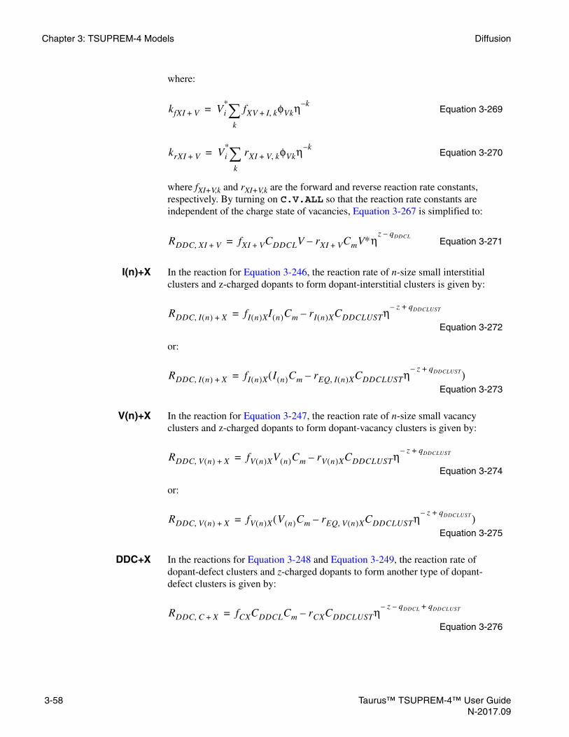
Chapter 3: TSUPREM-4 Models Diffusion

where:

Equation 3-269

Equation 3-270

where fXI+V,k and rXI+V,k are the forward and reverse reaction rate constants, respectively. By turning on C.V.ALL so that the reaction rate constants are independent of the charge state of vacancies, Equation 3-267 is simplified to:

Equation 3-271

I(n)+X In the reaction for Equation 3-246, the reaction rate of n-size small interstitial clusters and z-charged dopants to form dopant-interstitial clusters is given by:

Equation 3-272

or:

Equation 3-273

V(n)+X In the reaction for Equation 3-247, the reaction rate of n-size small vacancy clusters and z-charged dopants to form dopant-vacancy clusters is given by:

Equation 3-274

or:

Equation 3-275

DDC+X In the reactions for Equation 3-248 and Equation 3-249, the reaction rate of dopant-defect clusters and z-charged dopants to form another type of dopant-defect clusters is given by:

Equation 3-276

kfXI V+ Vi*

fXV I+ k, φVkη k–

k=

krXI V+ Vi*

rXI V+ k, φVkη k–

k=

RDDC XI V+, fXI V+ CDDCLV rXI V+ CmV∗ηz q– DDCL

–=

RDDC I n( ) X+, fI n( )XI n( )Cm rI n( )XCDDCLUSTηz– qDDCLUST+

–=

RDDC I n( ) X+, fI n( )X I n( )Cm rEQ I n( )X, CDDCLUSTηz– qDDCLUST+

–( )=

RDDC V n( ) X+, fV n( )XV n( )Cm rV n( )XCDDCLUSTηz– qDDCLUST+

–=

RDDC V n( ) X+, fV n( )X V n( )Cm rEQ V n( )X, CDDCLUSTηz– qDDCLUST+

–( )=

RDDC C X+, fCXCDDCLCm rCXCDDCLUSTηz– qDDCL– qDDCLUST+

–=

3-58 Taurus™ TSUPREM-4™ User GuideN-2017.09

Diffusion Chapter 3: TSUPREM-4 Models

or:

Equation 3-277

TransientPrecipitation

Model

When ACT.FULL or DDC.FULL models are turned on, the transient precipitation is simulated by solving the following equation:

Equation 3-278

where is given by:

Equation 3-279

is the equilibrium active concentration (Dopant Clustering Model, p. 3-38).

The time constant is given by:

for Equation 3-280

for Equation 3-281

Equations 3-278 is solved by two methods, that is, either the analytical method or the numerical method. The analytical method solves by assuming that does not vary within a time step. Likewise, with the ACT.TRAN model, Equations 3-120 which is similar to Equations 3-278 is always solved by the analytical method. Calculating the solution by the analytical method is much faster than iteratively solving the equation by the numerical method. However, when the total concentration is much larger than the equilibrium active concentration, that is,

and the boundary moves so quickly that the moving flux reduces a lot of the total concentration near surface, the total concentration can be smaller than the clustering concentration, which causes the negative active concentration. Thus, the numerical method which takes account of the moving boundary flux as well as the transient equilibrium active concentration is necessary in such a case. C0.NUMER, C0.ANALY and C0.HYBRI in the METHOD statement are the parameters to control the methods. C0.NUMER specifies to solve always by the numerical method while C0.ANALY does always by the analytical method. C0.HYBRI specifies that the numerical method is to be used when a boundary moves or temperature ramps; otherwise, the analytical method to be used.

RDDC C X+, fCX CDDCLCm rEQ CX, CDDCLUSTηz– qDDCL– qDDCLUST+

–( )=

Ccl0∂t∂

-------------Ccl0 Ccl0

*–

τcl0--------------------------–=

Ccl0*

Ca∗ DDCS.0 exp DDCS.E–

kT----------------------- Ca

∗ IIi

∗------ IFRACS DDCS.N

⋅+

C= wgb– Ccl1– Ccl2 DDC.N.DCDDCLUST Ccl0*

–––

Ca∗

τcl0

τcl0 C0.TF.0 C0.TF.E

kT-----------------------–

exp⋅= Ccl0 Ccl0*≤

τcl0 C0.TR.0 C0.TR.E

kT-----------------------–

exp⋅= Ccl0 Ccl0*>

Ccl0*

C Ccl0*∼

Taurus™ TSUPREM-4™ User Guide 3-59N-2017.09

Chapter 3: TSUPREM-4 Models Diffusion

Turning on the C0.TRAN parameter in the METHOD statement specifies to update C0 during the temperature ramp so that the active concentration must be always bigger than ACT.NI times the intrinsic carrier concentration, which is compatible with the ACT.TRAN model.

DDC andPrecipitationInitialization

The parameter DDCTOT.C defines the fraction of total dopant-defect clusters to implanted dopants in a crystalline region. The parameter DDCTOT.A defines the fraction of total dopant-defect clusters to the total clusters in the regrowth region. For correct initialization, these parameters must be defined when:

• DDC.T.0 of both and are nonzero and ACT.FULL is turned on

or:

• DDC.FULL is turned on

Hereinafter, it will be described by assuming that at least one of the above conditions is satisfied.

The parameters DDCFRACC and DDCFRACA define the fractions of a dopant-defect cluster of full dynamics to the total dopant-defect clusters in a crystalline region after implants and a regrowth region, that is, an amorphous region after implants, respectively.

The cluster solutions are initialized after implantation as follows;

Equation 3-282

where:

Equation 3-283

The parameter C0.INI.F determines the ratio of the initial precipitation to the implant dopant concentration subtracted by dopant-defect cluster concentration. Initializing a dopant-interstitial cluster requires the adjustment of the interstitial concentration. (See Cumulative Damage Model, p. 3-166.)

Equation 3-284

where:

Equation 3-285

Equation 3-286

Ccl1 Ccl2

Ccl0 Ccl0′

Ccl0Δ+=

Ccl0Δ 1 DDCTOT.C–( ) C0.INI.F Cimplant⋅ ⋅=

Ccl1 Ccl1′

Ccl1Δ+=

Ccl1Δ C1.INI.F DDCTOT.C⋅C1.INI.F C2.INI.F DDCFRACC+ +----------------------------------------------------------------------------------------------------- Cimplant⋅=

Ccl2 Ccl2′

Ccl2Δ+=

3-60 Taurus™ TSUPREM-4™ User GuideN-2017.09

Diffusion Chapter 3: TSUPREM-4 Models

where:

Equation 3-287

Equation 3-288

where:

Equation 3-289

The net capture of point-defects by clusters is given by:

Equation 3-290

Equation 3-291

Since the formation of dopant-defect clusters is limited by the number of point-defects, Equations , Equations and Equations are modified by:

Equation 3-292

Equation 3-293

Equation 3-294

Note: You may not define both nonzero DDC.I.N and DDC.V.N. But it is allowed to define both zero DDC.I.N and DDC.V.N, that is, dopant-only clusters. In such a case, .

In recrystallization during the anneal process following implant, clusters are initialized in an amorphous region as follows:

Equation 3-295

Equation 3-296

CΔ cl2C2.INI.F DDCTOT.C⋅

C1.INI.F C2.INI.F DDCFRACC+ +----------------------------------------------------------------------------------------------------- Cimplant⋅=

CDDC CDDC′

CDDCΔ+=

CDDCΔ DDCFRACC DDCTOT.C DDC.D.N⁄⋅C1.INI.F C2.INI.F DDCFRACC+ +--------------------------------------------------------------------------------------------------- Cimplant⋅=

IΔ IFRACM Ccl1Δ⋅ DDC.I.N CDDCΔ⋅+=

VΔ VFRACM Ccl2Δ⋅ DDC.V.N CDDCΔ⋅+=

Ccl1modΔ Ccl1 min 1.0 I IΔ⁄,( )⋅Δ=

Ccl2modΔ Ccl2 min 1.0 V VΔ⁄,( )⋅Δ=

CDDCmodΔ CDDC min 1.0

DDC.I.N I IΔ⁄⋅ DDC.V.N V VΔ⁄⋅+DDC.I.N DDC.V.N+

----------------------------------------------------------------------------------------, ⋅Δ=

CDDCmodΔ CDDCΔ=

Ccl0 1 DDCTOT.A–( ) Ccl total,⋅=

Ccl1C1FRAC.A DDCTOT.A⋅

C1FRAC.A C2FRAC.A DDCFRACA+ +----------------------------------------------------------------------------------------------------- Ccl total,⋅=

Taurus™ TSUPREM-4™ User Guide 3-61N-2017.09

Chapter 3: TSUPREM-4 Models Diffusion

Equation 3-297

Equation 3-298

When the boolean parameter CL.INI.A has been turned on, the total dopant clustering concentration in an amorphous region is initialized.

When ACT.NI > 0, the maximum active concentration in the regrowth region is limited by the minimum value among ACT.AMOR, ACT.NI.ni and Ca*. Ca* is taken into account only when the boolean EQACT.A parameter is turned on in the METHOD statement:

for ^EQACT.A:

Equation 3-299

for EQACT.A:

Equation 3-300

or:

when ACT.NI = 0

when

Equation 3-301

However, turning off CL.INI.A specifies to assume that all dopants are activated, that is, .

ACT.AMOR is the maximum active concentration in the recrystallized region of an amorphous region, and ACT.NI is the multiplication factor of the intrinsic carrier concentration, ni. C1FRAC.A denotes the fraction of to the total cluster concentration, . ACT.NI is corresponding to ACT.MIN in the ACT.TRAN model.

Having the DDC.FULL model disabled sets all DDCFRACC to zero, DDCTOT.C to C1.INI.F, and DDCTOT.A to C1FRAC.A.

In a crystalline region:

Equation 3-302

Ccl2C2FRAC.A DDCTOT.A⋅

C1FRAC.A C2FRAC.A DDCFRACA+ +----------------------------------------------------------------------------------------------------- Ccl total,⋅=

CDDCDDCFRACA DDCTOT.A DDC.D.N⁄⋅

C1FRAC.A DDCFRACA+------------------------------------------------------------------------------------ Ccl total,⋅=

Ccl total, max C min ACT.AMOR ACT.NI ni⋅,( ) 0.0,–( )=

Ccl total, max C min ACT.AMOR ACT.NI ni Ca∗,⋅,( ) 0.0,–( )=

Ccl total, max C ACT.AMOR 0.0,–( )= ACT.NI 0.0=

Ccl total, 0.0=

Ccl1

Ccl total,

Ccl0 min Ccl0_before_recrystallization Ccl0 min,,( )=

3-62 Taurus™ TSUPREM-4™ User GuideN-2017.09

Diffusion Chapter 3: TSUPREM-4 Models

where is calculated by:

Equation 3-303

and Equation 3-304

For the deposition of a doped material, all the dopants are assumed to be initially clustered. The precipitation is instantly dissolved at the very beginning of a post- thermal process with Equation 3-302.

Initialization forIn-Situ Doping

In-situ doping during epitaxial growth is performed with the EPITAXY or DEPOSIT commands. When a dopant is added to each incremental layer, the maximum of the initial active concentration of the dopant is set to the equilibrium active concentration by default. To change the initial active concentration, turn off the method for the initialization in equilibrium and specify the in-situ doping active concentration.

MATERIAL MAT=SILICON !EQACT.INIMPURITY IMP=BORON MAT=SILICON ACT.INSI=1E20

If ACT.INSI is not specified, the default value, 5E22, is used for boron. phosphorus, arsenic, and antimony.

Segregation of Impurities

The segregation of impurities at material interfaces is treated as a nonequilibrium process by TSUPREM-4.

Segregation Flux At an interface between materials and , the impurity flux from material to material (normal to the interface) is given by:

Equation 3-305

where:

• and are the concentrations in materials and , respectively.

• and are the charges

• is the interface transport coefficient.

• is the intrinsic equilibrium interface segregation coefficient.

Ccl0 min,

Camin DDCS.0 exp DDCS.EkT

-------------------– Camin

IIi

∗------ IFRACS

DDCS.N⋅+

C wgb– Ccl0 min,– Ccl1– Ccl2 DDC.D.NCDDCLUST––=

Camin min Ca∗ ACT.NI ni⋅,( )=

i j J i

j

J hCi

m-----η

qij Cjηqji–

=

Ci Cj i j

qij qji

h

m

Taurus™ TSUPREM-4™ User Guide 3-63N-2017.09

Chapter 3: TSUPREM-4 Models Diffusion

This expression represents the impurity flux in the diffusion equation at interfaces between different materials and between the ambient gas and the exposed surfaces of the simulation structure.

The segregation is based on the chemical impurity concentrations when the ACT.EQUI model is used and the active concentrations when other activation models are used. (When , the chemical concentrations are used in all cases.) For materials using the polycrystalline model, segregation at material interfaces is based on the concentration in the grain interior.

TransportCoefficient

The transport coefficient is given by:

Equation 3-306

SegregationCoefficient

The segregation coefficient defines the ratio in intrinsic equilibrium, when the interface impurity flux vanishes. The segregation coefficient is given by:

Equation 3-307

Fermi-LevelDependence

When the charge state of a dopant in a material is different from that in the neighbor material, the segregation of the charged dopant in the material i (or j) must depend on the Fermi-level for charge conservation. The charges and are defined by the SEG.CPOW parameter.

The coefficients TRANS.0, TRANS.E, SEG.0, SEG.E, and SEG.CPOW for each impurity and pair of materials are defined on the coefficient statements for impurities (see Chapter 4, IMPURITY, p. 4-281, Chapter 4, ANTIMONY, p. 4-350, Chapter 4, ARSENIC, p. 4-357, Chapter 4, BORON, p. 4-364, and Chapter 4, PHOSPHORUS, p. 4-371). For an interface between materials and , material

is specified by the MATERIAL parameter and material is specified with the/MATERIA parameter.

Moving-BoundaryFlux

There is an additional flux at oxidizing interfaces due to the consumption of silicon containing impurities. The flux is from the silicon into the oxide and is of magnitude , where is the impurity concentration on the silicon side of the interface and is the velocity of the interface.

Interface Trap Model

Assuming that there are trap sites at the interface between two adjacent materials, the dopant diffusing through the interface can be trapped into the trap site Reference [11]. The model is activated by specifying the ITRAP parameter on the METHOD statement.

V.COMPAT 6.4≤

h TRANS.0 exp TRANS.E–

kT---------------------------- ⋅=

Ci Cj⁄

m SEG.0 exp SEG.E–

kT--------------------- ⋅=

qij qji

i j

i j

vCSi CSi

v

3-64 Taurus™ TSUPREM-4™ User GuideN-2017.09

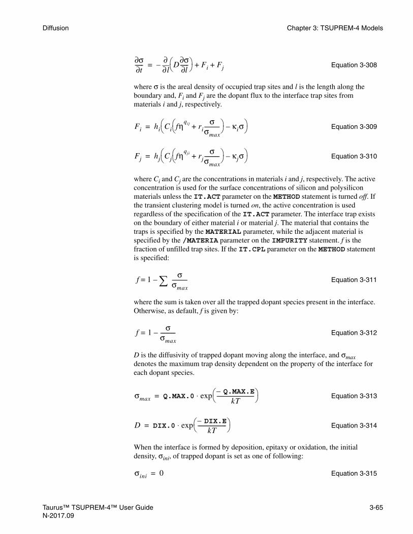
Diffusion Chapter 3: TSUPREM-4 Models

Equation 3-308

where σ is the areal density of occupied trap sites and l is the length along the boundary and, Fi and Fj are the dopant flux to the interface trap sites from materials i and j, respectively.

Equation 3-309

Equation 3-310

where Ci and Cj are the concentrations in materials i and j, respectively. The active concentration is used for the surface concentrations of silicon and polysilicon materials unless the IT.ACT parameter on the METHOD statement is turned off. If the transient clustering model is turned on, the active concentration is used regardless of the specification of the IT.ACT parameter. The interface trap exists on the boundary of either material i or material j. The material that contains the traps is specified by the MATERIAL parameter, while the adjacent material is specified by the /MATERIA parameter on the IMPURITY statement. f is the fraction of unfilled trap sites. If the IT.CPL parameter on the METHOD statement is specified:

Equation 3-311

where the sum is taken over all the trapped dopant species present in the interface. Otherwise, as default, f is given by:

Equation 3-312

D is the diffusivity of trapped dopant moving along the interface, and σmax denotes the maximum trap density dependent on the property of the interface for each dopant species.

Equation 3-313

Equation 3-314

When the interface is formed by deposition, epitaxy or oxidation, the initial density, σini, of trapped dopant is set as one of following:

Equation 3-315

σ∂t∂

------l∂

∂D

σ∂l∂

------ – Fi Fj+ +=

Fi hi Ci fηqij ri

σσmax-----------+

κiσ– =

Fj hj Cj fηqji rj

σσmax-----------+

κjσ– =

f 1σ

σmax-----------–=

f 1σ

σmax-----------–=

σmax Q.MAX.0 exp Q.MAX.E–

kT---------------------------- ⋅=

D DIX.0 exp DIX.E–

kT--------------------- ⋅=

σini 0=

Taurus™ TSUPREM-4™ User Guide 3-65N-2017.09

Chapter 3: TSUPREM-4 Models Diffusion

Equation 3-316

Equation 3-317

The initial density of trapped dopant is set by specifying one of parameters, IT.ZERO (Equation 3-315), IT.THERM (Equation 3-316), or IT.STEAD (Equation 3-317) on the METHOD statement. Equation 3-317 satisfies the steady state, Fi+Fj=0.

Note:If the impurity is first introduced by implantation, the initial value of the occupied trap density of the impurity is set to zero regardless of the above specification.

Assuming that the interface trap exists on the boundary of material i, hereinafter, the transport coefficients hi and hj are given by:

Equation 3-318

Equation 3-319

The ri and rj denote the ratio of detrapping rate to trapping rate at the interface with materials i and j, respectively, which are given by:

Equation 3-320

Equation 3-321

The detrapping of trapped dopant from an interface is determined by how many more dopants can be accepted into the material, as well as how many trapped dopants exist. For concentrations over critical concentration, no more detrapping occurs. SEG.SS and /SEG.SS specify that the critical concentrations are the same as the solid solubilities of dopant in materials i and j, respectively. SEG.SS and /SEG.SS may be applied only to the silicon or polysilicon material. The κi and κj are then given by:

Equation 3-322

σini Q.INI.0 exp Q.INI.E–

kT---------------------------- ⋅=

σini

σmaxf hiCi hjCj+( )hiCi 1 ri–( ) hjCj 1 rj–( ) σmax hiκi hjκj+( )+ +----------------------------------------------------------------------------------------------------------------=

hi TRANS.0 exp TRANS.E–

kT---------------------------- ⋅=

hj /TRANS.0 exp /TRANS.E–

kT------------------------------ ⋅=

ri RATIO.0 exp RATIO.E–

kT---------------------------- ⋅=

rj /RATIO.0 exp /RATIO.E–

kT------------------------------ ⋅=

κi ri

Css,i

σmax-----------, κj rj

Css,j

σmax----------- ==

3-66 Taurus™ TSUPREM-4™ User GuideN-2017.09

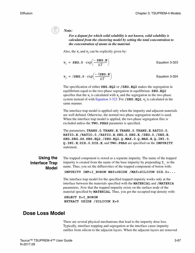
Diffusion Chapter 3: TSUPREM-4 Models

Note:For a dopant for which solid solubility is not known, solid solubility is calculated from the clustering model by setting the total concentration to the concentration of atoms in the material.

Also, the κi and κj can be explicitly given by:

Equation 3-323

Equation 3-324

The specification of either SEG.EQ2 or /SEG.EQ2 makes the segregation in equilibrium equal to the two-phase segregation in equilibrium. SEG.EQ2 specifies that the κi is calculated with κj and the segregation in the two-phase system instead of with Equation 3-323. For /SEG.EQ2, κj is calculated in the same manner.

The interface trap model is applied only when the impurity and adjacent materials are well defined. Otherwise, the normal two-phase segregation model is used. When the interface trap model is applied, the two-phase segregation flux is excluded unless the TWO.PHAS parameter is specified.

The parameters, TRANS.0, TRANS.E, TRANS.0, TRANS.E, RATIO.0, RATIO.E, /RATIO.0, /RATIO.E, SEG.0, SEG.E, /SEG.0, /SEG.E, SEG.SEG.SS, SEG.EQ2, /SEG.EQ2, Q.MAX.0, Q.MAX.E, Q.INI.0, Q.INI.E, DIX.0, DIX.E, and TWO.PHAS are specified on the IMPURITY statement.

Using theInterface Trap

Model

The trapped component is stored as a separate impurity. The name of the trapped impurity is created from the name of the base impurity by prepending I_ to the name. Thus, you set the diffusivities of the trapped component of boron with:

The interface trap model for the specified trapped impurity works only at the interface between the materials specified with the MATERIAL and /MATERIA parameters. Note that the trapped impurity exists on the surface node of the material specified by MATERIAL. Thus, you get the occupied trap density with:

Dose Loss Model

There are several physical mechanisms that lead to the impurity dose loss. Typically, interface trapping and segregation at the interface cause impurity outflux from silicon to the adjacent layers. When the adjacent layers are removed

κi SEG.0 exp SEG.E–

kT--------------------- ⋅=

κj /SEG.0 exp /SEG.E–

kT----------------------- ⋅=

IMPURITY IMP=I_BORON MAT=OXIDE /MAT=SILICON DIX.0=...

SELECT Z=I_BORONEXTRACT OXIDE /SILICON X=0

Taurus™ TSUPREM-4™ User Guide 3-67N-2017.09

Chapter 3: TSUPREM-4 Models Diffusion

later in the process flow, like a sacrificial oxide, the impurity trapped there is also removed. This means dose loss for the impurity that remains inside silicon wafer.

This section describes dose loss mechanism due to the impurity sweeping by the advancing epitaxial recrystallization front when an amorphized silicon layer is annealed. This effect has been observed for indium, where up to 80% of the dose can disappear during the epitaxial recrystallization of the amorphized layer. For arsenic, similarly fast dose loss has been reported, although not as dramatic as for indium.

A simple model can describe this effect. During epitaxial recrystallization of the amorphized layer, all indium above certain threshold concentration is swept by the advancing recrystallization front. This applies to all dopants that happen to be inside the amorphous layer, regardless of which ion was implanted.

Threshold concentration of 6e18 cm-3 was identified for indium for this purpose. The threshold concentration can be specified by parameter MAX.AMOR on the IMPURITY command. The values of MAX.AMOR parameter for the other dopants is set to a very high value of 5e22 cm-3.

Diffusion of Point Defects

This section describes the equations that model the diffusion of interstitials and vacancies in silicon. The modeling of point defects depends on the NSTREAMS, PD.PFLUX, PD.PTIME, and PD.PREC parameters on the METHOD statement (see p. 3-18). For NSTREAMS =1 (for example, if PD.FERMI is set on the METHOD statement), the interstitial and vacancy concentrations depend only on the Fermi level:

Equation 3-325

The point defect enhancement factors and in the equation for diffusion of impurities are unity (see Diffusion of Impurities, p. 3-18), and there is no enhancement (or retardation) of impurity diffusion due to oxidation.

EquilibriumConcentrations

The equilibrium concentrations and are given by:

Equation 3-326

Equation 3-327

Equation 3-328

I I*

= and V V*

=

M M′⁄ N N′⁄

I*

V*

I*

Ii* φIkη k–

k 2–=

2

= V*

Vi* φVkη k–

k 2–=

2

=

Ii*

FIsts CEQUIL.F Ii0*⋅ ⋅=

Vi*

FVsts CEQUIL.F Vi0*⋅ ⋅=

3-68 Taurus™ TSUPREM-4™ User GuideN-2017.09

Diffusion Chapter 3: TSUPREM-4 Models

Equation 3-329

where CEQUIL.0 and CEQUIL.E are parameters on the INTERSTITIAL and VACANCY statements.

PressureDependence

The factors FIsts and FVsts are applied only in silicon materials for which the stress history is modeled, and either the ST.EFORM model or the ST.PDEQ model is enabled in the METHOD statement. The activating volume, VCEQUIL has a dimension of A3 and is specified in the INTERSTI and VACANCY statements.

Equation 3-330

User-DefinedIsotropic

Multiplication

The point-defect concentration in intrinsic equilibrium can be multiplied by the parameter CEQUIL.F in the INTERSTI and VACANCY statements. Parameters values can be numbers or formulas. This allows you to define more complicated equilibrium models for point-defects.

Charge StateFractions

The charge state fractions and are given by:

Equation 3-331

Equation 3-332

Equation 3-333

Equation 3-334

Equation 3-335

Equation 3-336

Equation 3-337

Ii0*

and Vi0*

CEQUIL.0 exp CEQUIL.E–

kT------------------------------- ⋅=

FIsts and FVsts expp VCEQUIL⋅–

kT--------------------------------- =

φIk φVk

φIk

φ′Ik

φ′Ik

k 6–=

6

---------------------= and φVk

φ′Vk

φ′Vk

k 6–=

6

-----------------------=

φ′I 2–( ) and φ′V 2–( ) DNEG.0 exp DNEG.E–

kT------------------------ ⋅=

φ′I 1–( ) and φ′V 1–( ) NEG.0 exp NEG.E–

kT--------------------- ⋅=

φ′I0 and φ′V0 NEU.0 exp NEU.E–

kT--------------------- ⋅=

φ′I1 and φ′V1 POS.0 exp POS.E–

kT--------------------- ⋅=

φ′I2 and φ′V2 DPOS.0 exp DPOS.E–

kT------------------------ ⋅=

φ′Ik and φ′Vk FRAC.0 exp FRAC.E–

kT------------------------ ⋅=

Taurus™ TSUPREM-4™ User Guide 3-69N-2017.09

Chapter 3: TSUPREM-4 Models Diffusion

The last form gives the fractions for arbitrary charge states . The parameters for interstitials are specified on the INTERSTITIAL statement (see Chapter 4, INTERSTITIAL, p. 4-319), while the parameters for vacancies are specified on the VACANCY statement (see Chapter 4, VACANCY, p. 4-336); the charge state is specified by the C.STATE parameter. Note that the defect concentrations are not actually calculated when NSTREAMS=1; the values and

are used when the interstitial and vacancy concentrations are printed or plotted.

Point DefectDiffusion

Equations

For NSTREAMS =3 (for example, if PD.TRANS or PD.FULL is set on the METHOD statement), the equations for point defect diffusion are solved:

Equation 3-338

Equation 3-339

Equation 3-340

where:

• and are the concentrations of dopant-interstitial and dopant-vacancy pairs defined in Diffusion of Impurities, p. 3-18.

6– k 6≤ ≤

k

I*

V*

∂ I Ic Idds+ +( )∂t

------------------------------------∂M∂t

--------+ ∇ DII*∇ I

I*

---- Jm+–⋅

Gp Rb Rti RsIcI RlIcI–– RsVcI RlVcI– Rl–– Rdd–

R DDCMRDDC C I+, RDDC I M+, RDDC X I+,––––

––+

–=

∂ V Vc+( )∂t

----------------------∂N∂t-------+ ∇ DVV

*∇ V

V*

------ Jn+–

Gp Rb– RsVcV RlVcV–– RsIcV RlIcV– Rdv–

R DDCN– RDDC C V+, RDDC V N+, RDDC X V+,–––

–+

⋅–=

Gp

KmvVV∗------

Km KmvVV∗------+

------------------------------∂M∂t

-------- ∇ Jm RDDCM+⋅+

KniII∗-----

Kn KniII∗-----+

--------------------------∂N∂t------- ∇ Jn RDDCN+⋅+ +

=

M N

3-70 Taurus™ TSUPREM-4™ User GuideN-2017.09

Diffusion Chapter 3: TSUPREM-4 Models

• and are the corresponding fluxes.

• and are the concentrations of interstitials and vacancies in small clusters (see Equilibrium Small Clustering, p. 3-87).

• is the concentration of interstitials in small dopant-defect clusters (see Activation of Impurities, p. 3-35).

• , , , and model the loss of free interstitials to dopant-defect clusters (Dopant-Interstitial Clustering Model, p. 3-39), bulk recombination (Recombination of Interstitials With Vacancies, p. 3-74), interstitial traps (Interstitial Traps, p. 3-80), dislocation loops (Dislocation Loop Model, p. 3-97), respectively. The term model the loss of free vacancies to the small interstitial clusters(Transient Small Clustering, p. 3-88) and {311} defects (Interstitial Clustering Models, p. 3-81).

• , , and model the loss of free interstitials to small interstitial clusters (Transient Small Clustering, p. 3-88), large interstitial clusters, that is, {311} defects (Interstitial Clustering Models, p. 3-81), small vacancy clusters (Transient Small Clustering, p. 3-93), large vacancy clusters (Large Clustering Model, p. 3-90).

• , , and model the loss of free vacancies to small vacancy clusters (Transient Small Clustering, p. 3-93), large vacancy clusters (Large Clustering Model, p. 3-90), small interstitial clusters (Transient Small Clustering, p. 3-88), large interstitial clusters, that is, {311} defects (Interstitial Clustering Models, p. 3-81).

• and term model the loss of free interstitials and vacancies to the dopant-defect clusters. (DDC+I, p. 3-43, DDC+V, p. 3-43), XV+I, p. 3-57, and XI+V, p. 3-57.

• and model the loss of free interstitials to dopant-defect clusters by reacting with a dopant-interstitial pair and another dopant-defect cluster respectively. (M+I, p. 3-46 and N+V, p. 3-47).

• and term model the loss of free interstitials and vacancies by the reaction with the mobile dopant to form the dopant-defect clusters. These terms are only applicable for the impurity which diffuses without pairing to point-defects. (X+I, p. 3-56 and X+V, p. 3-56)

•

(Full Dynamics of Dopant-Defect Clustering, p. 3-40)

•

(Full Dynamics of Dopant-Defect Clustering, p. 3-40)

The sums are taken over all dopant species present in the structure. The and terms are included only if PD.PTIME is true (set on the METHOD statement, directly or by specifying PD.FULL); otherwise, they are set to 0. Likewise, the and terms are included only if PD.PFLUX is true (set on the METHOD statement, directly or by specifying PD.FULL).

Jm Jn

Ic Vc

I dsd

Rdd Rb Rt Rl

RsIcI RlIcI RsVcI RlVcI

RsVcV RlVcV RsIcV RlIcV

RDDC C I+, RDDC C V+,

RDDC I M+, RDDC C I+,

RDDC X I+, RDDC X V+,

RDDCM RDDC S M+, R+ DDC I M+, RDDC In M+, 2RDDC M M+,RDDC C M+, R+ DDC M N+, RDDC Vn 1+ M+, RDDC XI2 V+,–

+ ++ +

=

RDDCN RDDC S N+, R+ DDC V N+, RDDC In 1+ N+, 2RDDC N N+,RDDC C N+, R+ DDC M N+, RDDC Vn N+, RDDC XV2 I+,–

+ ++ +

=

M N

Jm

Jn

Taurus™ TSUPREM-4™ User Guide 3-71N-2017.09

Chapter 3: TSUPREM-4 Models Diffusion

For NSTREAMS =5 or PD.5STR, the equations for point defect diffusion are solved:

Equation 3-341

Equation 3-342

Interstitial andVacancy

Diffusivities

and are the diffusivities of interstitials and vacancies, respectively, given by:

Equation 3-343

Equation 3-344

where and are specified by:

Equation 3-345

∂ I Ic Idds+ +( )∂t

------------------------------------ ∇ DII*∇ I

I*

---- –

⋅ Gm Rm–( ) Gni Rni–( )

R– b

––

Rti RsIcI RlIcI–– R– sVcI RlVcI– Rl– Rdd–

RDDC C I+, RDDC I M+, RDDC X I+,–––

–

–=

∂ V Vc+( )∂t

------------------------ ∇ DVV*∇ V

V*

------ –

⋅ Gn Rn–( ) Gmv Rmv–( )

R– b

–

RsVcV RlVcV––

–

RsIcV R– lIcV–

RDDC C V+, RDDC V N+, RDDC X V+,–––

–=

DI DV

DI FDIsts D.FACTOR D.F11 0

0 D.F22

DIkφIkη k–

k

φIkη k–

k

−−−−−−−−−−−−−−−−−−−⋅ ⋅ ⋅ =

DV FDVsts D.FACTOR D.F11 0

0 D.F22

DVkφVkη k–

k

φVkη k–

k

−−−−−−−−−−−−−−−−−−−−⋅ ⋅ ⋅=

DIk DVk

DIk and DVk D.0 exp D.E–kT

-------------- ⋅ DC.0 exp

DC.E–kT

------------------ ⋅×=

3-72 Taurus™ TSUPREM-4™ User GuideN-2017.09

Diffusion Chapter 3: TSUPREM-4 Models

where DC.0 and DC.E are specified for . D.0, D.E, DC.0, DC.E, and C.STATE for and are specified on the INTERSTITIAL (Chapter 4, INTERSTITIAL, p. 4-319) and VACANCY (Chapter 4, VACANCY, p. 4-336) statements, respectively. DC.0 and DC.E can also be set for all charge states by specifying C.ALL.

Two approaches can be used to specify the diffusivity of point defects:

1. D.0 (in cm2/s or microns2/min) and D.E can be used to specify the basic dif-fusivity while DC.0 (unitless) and DC.E specify relative diffusivities of the various charge states

2. DC.0 (in cm2/s or microns2/min) and DC.E can be used to specify the diffusivities of the various charge states while DC.0 (unitless) and DC.E specify a scale factor for adjusting the total diffusivity.

Note:While theoretical calculations suggest that the point defect diffusivities may depend on the Fermi level, this dependence has not been experimentally characterized. By default, all of the DC.0 are set to 1.0 and all of the DC.E are set to zero, so the diffusivity (determined by the values of D.0 and D.E using approach 1 above) is independent of the Fermi level.

PressureDependence

The factor FDIsts and FDVsts is applied only for diffusion in silicon materials for which the stress history is modeled, and the ST.DIFF model is enabled. The activating volume, VD has a dimension of A3 and is specified on the INTERSTI and VACANCY statements. The parameters ST.HIST and ST.DIFF for setting stress history and stress dependent diffusion are specified on the METHOD statement.

Equation 3-346

User-DefinedIsotropic

Multiplication

The diffusivities can be multiplied by the parameter D.FACTOR in the INTERSTI and VACANCY statements. Parameters values can be numbers or formulas. This allows you to define more complicated point-defect diffusivity models.

User-DefinedAnisotropic

Multiplication

To provide the modeling capability for an anisotropic point-defect diffusion, the user-specified tensor expression can be taken. It describes the anisotropic diffusion path, which is given by the parameters D.F11 and D.F22 in the INTERSTI and VACANCY statement. Each parameter can be given by any formula expression.

Reaction of PairsWith Point

Defects

In the PD.FULL model, the terms are the result of dopant-defect pairs reacting with dopants. Normally, when dopant-interstitial pairs break up, they produce an interstitial, which is accounted for by the and terms in Equation 3-338.

C.STATE k=DI DV

FDIsts and FDVsts expp VD⋅–kT

----------------- =

Gp

M Jm

Taurus™ TSUPREM-4™ User Guide 3-73N-2017.09

Chapter 3: TSUPREM-4 Models Diffusion

However, when dopant-assisted recombination is dominant, dopant-interstitial pairs are destroyed by absorbing a vacancy rather than producing an interstitial. Under these circumstances, the term cancels the and terms in Equation 3-338 and subtracts them from Equation 3-339 instead. Similarly, dopant-vacancy pairs can either produce a vacancy or absorb an interstitial when they dissolve.

Recombinationof Interstitials

With Vacancies

The net recombination rate of interstitials with vacancies in the bulk silicon is given by:

Equation 3-347

Equation 3-348

for true PD.PREC in the PD.FULL model, otherwise

where:

• is the substitutional dopant concentration.

• , , and are described in Diffusion of Impurities, p. 3-18.

• and are described in Equilibrium Small Clustering, p. 3-87.

Again, the sums are taken over all dopant species. The and terms model dopant-assisted recombination; they are included only if PD.PREC is true (set on the METHOD statement, directly or by specifying PD.FULL); otherwise, they are set to zero.

The bulk recombination factor is specified by:

Equation 3-349

where KB.0 and KB.E are parameters on the INTERSTITIAL statement.

The factor FIV describes the dependence of the recombination rate on the charge states of the point defects:

Equation 3-350

Equation 3-351

Gp M Jm

Rb Kb FIV FcV FIc+ +( ) II∗-----

VV∗------ 1–

Rprec+=

Rprec

KmKmv

Km KmvVV∗------+

------------------------------KnKni

Kn KniII∗-----+

--------------------------+

S II∗-----

VV∗------ 1–

=

Rprec 0=

S C M– N–=

Km Kn Kmv Kni

FIc FcV

Kmv Kni

Kb

Kb KB.0 exp KB.E–kT

------------------ ⋅=

FIV Ii∗Vi

∗ KIV jk, φIjηj– φVkη k–

j k, α⁄=

KIV jk, KIV.0 exp KIV.E–

kT--------------------- ⋅=

3-74 Taurus™ TSUPREM-4™ User GuideN-2017.09

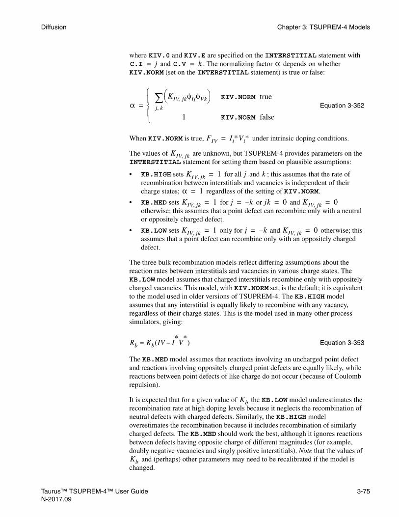
Diffusion Chapter 3: TSUPREM-4 Models

where KIV.0 and KIV.E are specified on the INTERSTITIAL statement with and . The normalizing factor depends on whether

KIV.NORM (set on the INTERSTITIAL statement) is true or false:

Equation 3-352

When KIV.NORM is true, under intrinsic doping conditions.

The values of are unknown, but TSUPREM-4 provides parameters on the INTERSTITIAL statement for setting them based on plausible assumptions:

• KB.HIGH sets for all and ; this assumes that the rate of recombination between interstitials and vacancies is independent of their charge states; regardless of the setting of KIV.NORM.

• KB.MED sets for or and otherwise; this assumes that a point defect can recombine only with a neutral or oppositely charged defect.

• KB.LOW sets only for and otherwise; this assumes that a point defect can recombine only with an oppositely charged defect.

The three bulk recombination models reflect differing assumptions about the reaction rates between interstitials and vacancies in various charge states. The KB.LOW model assumes that charged interstitials recombine only with oppositely charged vacancies. This model, with KIV.NORM set, is the default; it is equivalent to the model used in older versions of TSUPREM-4. The KB.HIGH model assumes that any interstitial is equally likely to recombine with any vacancy, regardless of their charge states. This is the model used in many other process simulators, giving:

Equation 3-353

The KB.MED model assumes that reactions involving an uncharged point defect and reactions involving oppositely charged point defects are equally likely, while reactions between point defects of like charge do not occur (because of Coulomb repulsion).

It is expected that for a given value of the KB.LOW model underestimates the recombination rate at high doping levels because it neglects the recombination of neutral defects with charged defects. Similarly, the KB.HIGH model overestimates the recombination because it includes recombination of similarly charged defects. The KB.MED should work the best, although it ignores reactions between defects having opposite charge of different magnitudes (for example, doubly negative vacancies and singly positive interstitials). Note that the values of

and (perhaps) other parameters may need to be recalibrated if the model is changed.

C.I j= C.V k= α

αKIV jk, φIjφVk

j k, KIV.NORM true

1 KIV.NORM false

=

FIV Ii∗Vi

∗=

KIV jk,

KIV jk, 1= j k

α 1=

KIV jk, 1= j k–= jk 0= KIV jk, 0=

KIV jk, 1= j k–= KIV jk, 0=

Rb Kb= IV I*

V*

–( )

Kb

Kb

Taurus™ TSUPREM-4™ User Guide 3-75N-2017.09

Chapter 3: TSUPREM-4 Models Diffusion

Note:Versions of the program prior to 1999.2 did not use the KIV.0, KIV.E, or KIV.NORM parameters, but some of them did use KB.LOW, KB.MED, and KB.HIGH. If compatibility with those versions is required, use KIV.NORM when KB.LOW is used and ^KIV.NORM when KB.MED is used, or use V.COMPAT=1998.4 on the OPTION statement.

Absorption byTraps, Clusters,and Dislocation

Loops

is the rate of absorption of interstitials at stationary interstitial trapping sites; is given by Equation 3-374 in Interstitial Traps, p. 3-80. is the rate of absorption by interstitial clusters (see Interstitial Clustering Models, p. 3-81). is the rate of absorption of interstitials by dislocation loops (see Dislocation Loop Model, p. 3-97).

Injection and Recombination of Point Defects at Interfaces

Recombination of interstitials and vacancies at interfaces with other materials is modeled as Reference [12].

Equation 3-354

where:

• is the local concentration of interstitials or vacancies.

• is the equilibrium concentration of interstitials or vacancies.

• is the surface recombination rate.

• KSURF.F is the expression string which is specified in the INTERSTITIAL or VACANCY statements.

SurfaceRecombination

Velocity Models

There are three models for the surface recombination velocity, specified by the V.MAXOX, V.INITOX, and V.NORM parameters on the INTERSTITIAL and VACANCY statements. In each case, the surface recombination rate depends on the motion of the interface due to oxidation:

Equation 3-355

Equation 3-356

Equation 3-357

Rt Rt

Rc

Rl

Rs KSURF.F K⋅ s C C*

–( )=

C

C*

Ks

Ks Ksurf Ksvel Ksurf–( ) vvmax---------- Kpow

+= V.MAXOX model( )

Ks Ksurf 1 Ksrat+v

vinit--------- Kpow

= V.INITOX model( )

Ks Ksurf Ksvelv

vnorm------------- Kpow

+= V.NORM model( )

3-76 Taurus™ TSUPREM-4™ User GuideN-2017.09

Diffusion Chapter 3: TSUPREM-4 Models

where is the local velocity of the interface and , and are specified by:

Equation 3-358

Equation 3-359

Equation 3-360

Equation 3-361

where KSURF.0, KSURF.E, KSVEL.0, KSVEL.E, KSRAT.0, KSRAT.E, KPOW.0, and KPOW.E are parameters on the INTERSTITIAL and VACANCY statements.

The three models differ primarily in the normalizing factor for the interface velocity. This section describes the differences between the models, and their advantages and disadvantages.

V.MAXOX Model The V.MAXOX model (the model used in releases of TSUPREM-4 prior to version 6.0) uses , the maximum y component of interface velocity in the structure. The disadvantage of this model is that the normalization factor varies with time and oxidation conditions so that the peak recombination velocity does not depend on the oxidation rate.

V.INITOX Model The V.INITOX model (the model used in SUPREM-IV from Stanford University and the University of Florida) corrects the time dependence by using a normalization factor:

Equation 3-362

where and are the linear and thin regime oxidation rates defined in Oxidation, p. 3-99. Thus is the initial oxidation rate of a bare silicon surface. This normalizing factor gives a good time dependence, but the initial surface recombination velocity is still independent of the oxidation conditions such as wet or dry ambient, pressure, or presence of HCl.

V.NORM Model The V.NORM model provides both the time dependence and the dependence on the oxidation conditions by using a constant normalizing factor specified by you:

Equation 3-363

v Ksurf Ksvel Ksrat

Ksurf KSURF.0 exp KSURF.E–

kT---------------------------- ⋅=

Ksvel KSVEL.0 exp KSVEL.E–

kT---------------------------- ⋅=

Ksrat KSRAT.0 exp KSRAT.E–

kT---------------------------- ⋅=

Kpow KPOW.0 exp KPOW.E–

kT------------------------ ⋅=

vmax

vinitBA--- rthin+=

BA--- rthin

vinit

vnorm VNORM.0 exp VNORM.E–

kT---------------------------- ⋅=

Taurus™ TSUPREM-4™ User Guide 3-77N-2017.09

Chapter 3: TSUPREM-4 Models Diffusion

where VNORM.0 and VNORM.E are parameters on the INTERSTITIAL and VACANCY statements.

TrappedNitrogen–

DependentSurface

Recombination

The point defect recombination at interfaces depends on trapped nitrogen atoms. Since the recombination rate at interfaces is proportional to the number of kink sites which is supposed to be reduced by trapping nitrogen, the recombination of interstitials and vacancies at interfaces is given by:

Equation 3-364

where N.MAX.0 and N.MAX.E are parameters on the INTERSTITIAL and VACANCY statements. The model is taken into account by specifying the PD.NREC parameter on the METHOD statement.

Injection Rate At moving interfaces there can be injection of interstitials and/or vacancies into the silicon. The injection rate is given either as a function of the interface velocity or by an analytical function of time, depending on whether the GROWTH parameter has been specified on the INTERSTITIAL or VACANCY statement. The injection rate also depends on which of the injection/recombination models (V.MAXOX, V.INITOX, or V.NORM) is specified.

When GROWTH is true, the injection is calculated based on the local interface velocity:

Equation 3-365

Equation 3-366

Equation 3-367

where:

• THETA.F is the expression string.

• VMOLE is the number of silicon atoms per cubic centimeter.

• is the fraction of silicon atoms injected.

• is the local interface velocity.

• , , and are given by Equations 3-361, 3-362, and 3-363, respectively.

R KSURF.F K⋅ s 1σN

N.MAX.0N.MAX.E

kT-----------------------–

exp-----------------------------------------------------------------–

C C*

–( )=

Gs

Gs THETA.F VMOLE θvKpow⋅ ⋅= V.MAXOX model( )

Gs THETA.F VMOLE θvv

vinit--------- Gpow

⋅ ⋅= V.INITOX model( )

Gs THETA.F VMOLE θvv

vnorm------------- Gpow

⋅ ⋅= V.NORM model( )

θ

v

Kpow vinit vnorm

3-78 Taurus™ TSUPREM-4™ User GuideN-2017.09

Diffusion Chapter 3: TSUPREM-4 Models

The values of and are specified as:

Equation 3-368

Equation 3-369

where THETA.F, THETA.E, GPOW.0, and GPOW.E are parameters on the INTERSTITIAL and VACANCY statements.

If GROWTH is false, the analytical model is used:

Equation 3-370

Equation 3-371

where is the time into the oxidation step and and are given by:

Equation 3-372

Equation 3-373

where THETA.F, A.0, A.E, T0.0, and T0.E are parameters on the INTERSTITIAL and VACANCY statements. Note that this model must be calibrated for a particular starting structure and growth conditions.

The GROWTH model is normally used for injection of interstitials at an oxide/silicon interface. The analytical model is used with to disable injection of interstitials at other interfaces and injection of vacancies at all interfaces.

Moving-Boundary Flux

There is an additional flux at oxidizing interfaces due to the consumption of silicon containing point defects. The flux is directed out of the silicon and is of magnitude , where is the interstitial or vacancy concentration in the silicon and is the velocity of the interface. Point defects are not modeled in materials other than silicon, so point defects removed in this fashion have no further effect on the simulation.

θ Gpow

θ THETA.0 exp THETA.E–

kT---------------------------- ⋅=

Gpow GPOW.0 exp GPOW.E–

kT------------------------ ⋅=

Gs THETA.FA

T0 t+( )Kpow

---------------------------⋅= V.MAXOX model( )

Gs THETA.F A⋅( ) T0 t+( )Gpow=( ) V.INITOX and V.NORM models( )

t A T0

A A.0 exp A.E–kT

-------------- ⋅=

T0 T0.0 exp T0.E–kT

------------------ ⋅=

A.0 0=

vCSi CSi

v

Taurus™ TSUPREM-4™ User Guide 3-79N-2017.09

Chapter 3: TSUPREM-4 Models Diffusion

Interstitial Traps

The rate of absorption of interstitials at stationary trapping sites is given by References [13] and [14]:

Equation 3-374

where:

• is the concentration of filled interstitial traps.

• is the concentration of empty traps.

• and are the forward and reverse rates for the trap-filling reaction.

In equilibrium, the forward and reverse reactions proceed at equal rates giving:

Equation 3-375

where and are the equilibrium concentrations of filled and empty traps, respectively. Thus, Equation 3-374 becomes:

Equation 3-376

The total number of traps is given by:

Equation 3-377

where TRAP.CON is a parameter on the INTERSTITIAL statement. The reaction rate and equilibrium concentration of empty traps are given by:

Equation 3-378

Equation 3-379

where K.TRAP.0, K.TRAP.E, F.TRAP.0, and F.TRAP.E are parameters on the INTERSTITIAL statement.

Enabling,Disabling, and

Initialization

The interstitial trap model is enabled by setting TRAP.CON to a nonzero value and disabled by setting TRAP.CON to zero. The empty trap concentration is initialized to its equilibrium value at the start of the first diffusion step (DIFFUSION or EPITAXY statement) after the trap model is first enabled. In some cases it may be desirable to initialize the empty trap concentration to a value

Rt

∂TF

∂t--------- kfTEI krTF–= =

TF

TE

kf kr

kr

kfTE*

I*

TF*

---------------=

TF*

TE*

Rt

∂TF

∂t--------- kf TEI

TE*

I*

TF*

-----------TF–= =

TT TF TE+ TF*

TE*

+ TRAP.CON= = =

kf K.TRAP.0 exp K.TRAP.EkT

--------------------------– ⋅=

TE*

F.TRAP.0 exp F.TRAP.EkT

--------------------------– TRAP.CON×⋅=

TE

TE*

3-80 Taurus™ TSUPREM-4™ User GuideN-2017.09

Diffusion Chapter 3: TSUPREM-4 Models

smaller than its equilibrium value. This can be accomplished by first setting to the desired initial concentration of empty traps, doing a short diffusion (with TRAP.CON set nonzero to enable the trap model), then setting to the actual equilibrium concentration of empty traps.

Interstitial Clustering Models

TSUPREM-4 includes two models for the formation and dissolution of interstitial clusters ({311} or {113} defects). These clusters play an important part in transient-enhanced diffusion (TED) of impurities following ion implantation. The main effect of the models is to delay the onset of TED at low temperatures and to distribute the diffusion enhancement over a longer period of time. This eliminates the excessive diffusion at low temperatures that is predicted by older versions of TSUPREM-4.

The two interstitial clustering models are distinguished by the number of equations used to characterize the population of clusters. The 1-moment model uses a single equation to calculate the total number of interstitials bound in clusters. The 2-moment model uses an additional equation to calculate the number of clusters, and thus contains information on the size distribution of the clusters. All other things being equal, a 2-moment model should provide more flexible modeling and give more accurate results, but in practice the obtainable accuracy depends on the form of the model as well as on the number of moments. The 1-moment model in TSUPREM-4 is very general and can be adjusted to agree well with measured data. The 2-moment model is more constrained by theoretical concerns and is less flexible; while it can achieve reasonable agreement with experiment, it does not appear to have any advantages over the 1-moment model at present.

In addition to the model of {311} large interstitial clustering, TSUPREM-4 includes the two small interstitial clustering models, that is, the equilibrium model and the transient model. The transient small interstitial clustering model provides the full dynamics of the interstitial clusters. The boolean parameter CL.FULL specifies to use the transient small interstitial clustering model.

1-MomentClustering Model

The kinetics of {311} formation and dissolution are not well understood, and several models have been proposed (for example, Reference [15]). TSUPREM-4, therefore, uses a generalized model that includes many of the proposed models as subsets.

Equation 3-380

where is the concentration of clustered interstitials, and and describe cluster interaction with interstitials and vacancies, respectively. The

TE*

TE*

CIc∂t∂

----------- RIcI RIcV–=

CIc RIcI RIcV

Taurus™ TSUPREM-4™ User Guide 3-81N-2017.09

Chapter 3: TSUPREM-4 Models Diffusion

interstitial interaction includes three terms describing the nucleation, the clustering of interstitials and one describing the declustering:

for ^CL.FULL Equation 3-381

or:

for CL.FULL Equation 3-382

The first term in Equation 3-381 models the nucleation of the interstitial clusters at high interstitial supersaturation, which is given by:

Equation 3-383

where is the concentration of unclustered interstitials, and is the equilibrium concentration of interstitials.

When the CL.FULL model is set, the smallest large cluster forms when the small cluster I(max) captures one free interstitial by the reaction rate (Transient Small Clustering, p. 3-88). The second term models growth and dissolution of the large interstitial clusters by consuming and emitting free interstitials.

Equation 3-384

The vacancy interaction includes the one recombination and one generation term, as well as the reaction with the interstitial small clusters (only for the CL.FULL model):

for ^CL.FULL Equation 3-385

or:

for CL.FULL Equation 3-386

is the reaction rate of small interstitial clusters with vacancies (Transient Small Clustering, p. 3-88).

Equation 3-387

where is the concentration of free vacancies, and is the equilibrium concentration of vacancies. The first term models dissolution of the interstitial

RIcI RsIcI RlIcI+=

RIcI max 1+( )RsIcI max 1+( ) RlIcI+=

RsIcI

RsIcI KfiICL.IF

I∗CL.ISF-----------------------=

I I∗

RsIc max 1+( )RlIcI

RlIcI KfcICL.IFC

I∗CL.ISFC-------------------------- CIc αI+( )CL.CF KrCIc

CL.CR–=

RIcV RlIcV=

RIcV max 1+( )RsIcV max 1+( ) RlIcV+=

RsIcV max 1+( )

RlIcV KrvVCLI.VRC

V∗CLI.VSRC------------------------------CIc

CLI.CRKfvV∗CLI.VSFCCIc

CLI.CF–=

V V∗

3-82 Taurus™ TSUPREM-4™ User GuideN-2017.09

Diffusion Chapter 3: TSUPREM-4 Models

clusters by consuming vacancies. The second term models emission of vacancies by the interstitial clusters. The reactions constants are given by:

Equation 3-388

Equation 3-389

Equation 3-390

Equation 3-391

Equation 3-392

and , CL.IF, CL.ISF, CL.IFC, CL.ISFC, CL.CF, CL.CR, CL.KF.0, CL.KF.E, CL.KFC.0, CL.KFC.E, CL.KR.0, and CL.KR.E are parameters specified on the INTERSTITIAL statement. Besides, CLI.KR.0, CLI.KR.E, CLI.KF.0, CLI.KF.E, CLI.VRC, CLI.VSRC, CLI.CR, CLI.VSFC and CLI.CF are parameters specified on the VACANCY statement.

The changes in are accompanied by corresponding inverse changes in . Thus clustering reduces the number of free interstitials, while the dissolution of clusters releases interstitials.

The clustered interstitial concentration is initialized to the value specified for ABS.ERR (109/cm3 in silicon) or to the equilibrium value determined by Initialization of Large Point-Defect Clusters, p. 3-95 when the point defect models are first activated. After that, the concentration is determined by Equation 3-380.

Choosing ModelParameters

The interstitial clustering model is designed to work automatically, but for correct operation suitable parameter values must be chosen. Parameters for the model are set on the INTERSTITIAL and VACANCY statements specifying MATERIAL=SILICON as the material. Parameters should be chosen so that:

• Clusters form rapidly when the interstitial concentration is very high (that is, following an implant).

• Clusters decay at a suitable rate when the interstitial concentration is low.

• There is a small but nonzero concentration of clustered interstitials at equilibrium. This is required for numerical reasons, and may be needed to start the clustering process following a subsequent implant.

• The clustering model does not interfere with simulations of high-concentration diffusion, oxidation-enhanced diffusion, or other situations in which nonequilibrium interstitial concentrations may be present.

Kfi CL.KF.0CL.KF.E

kT-----------------------–

exp⋅=

Kfc CL.KFC.0CL.KFC.E

kT--------------------------–

exp⋅=

Kr CL.KR.0CL.KR.E

kT-----------------------–

exp⋅=

Krv CLI.KR.0CLI.KR.E

kT--------------------------–

exp⋅=

Kfv CL.KFV.0CL.KFV.E

kT--------------------------–

exp⋅=

α CL.KFC=

CIc I

CIc

Taurus™ TSUPREM-4™ User Guide 3-83N-2017.09

Chapter 3: TSUPREM-4 Models Diffusion

• The clustering model is numerically well behaved.

To obtain clustering following an implant, either the or term (or both) must be nonzero. For rapid clustering in response to an excess of interstitials, CL.IF, CL.IFC, and/or CL.CF must be set appropriately; larger values increase the dependence of the clustering rate on the interstitial concentration. Use CL.ISF and CL.ISFC to modify the clustering rate at high doping concentrations.

Dissolution of clusters and the release of interstitials requires a nonzero term. The parameter CL.CR must be greater than zero to avoid numerical difficulties (a value of 1.0 is typical). The forward reaction terms are also active during dissolution, so the net dissolution rate depends on the and terms as well as on the term.

The clustering model should also be examined to determine its impact on high-concentration diffusion (with PD.FULL) or OED. In either of these cases, excess interstitials could produce clustering, which can affect the diffusion of impurities.

The interstitial clustering model has been designed to be numerically well behaved when used with “reasonable” parameter values. In general this means that the clustering and dissolution rates must not be too large and the concentration of clustered interstitials must approach a reasonable value in equilibrium. In practice, it has been found that parameter values that give physically reasonable results are numerically well behaved.

The default parameter values use only the and terms. They have been chosen to fit the clustering data of Poate, et al. Reference [16] when used with the default values of the point defect parameters.

Using the Model The model is enabled by using the CL.1M parameter on the INTERSTITIAL statement:

INTERST MAT=SILICON CL.1M

The model is enabled by default. To disable the model use:

INTERST MAT=SILICON CL.NONE

The concentration of clustered interstitials is obtained by specifying the name cl_interst in the SELECT statement:

SELECT Z=LOG10(CL_INTERST)

In Synopsys TCAD’s graphical post-processing programs and in TIF files, the name clInterst is used.

2-MomentInterstitial

Clustering Model

The 2-moment interstitial clustering model, based on the work of Gencer and Dunham Reference [18], includes the nucleation and growth of {311} clusters, Ostwald ripening and decay of clusters, and conversion of {311} clusters into dislocation loops. The model calculates the first two moments of the size distribution of interstitial clusters, that is, the number of clusters and the number

Kfi Kfc

Kr

Kfi KfcKr

Kfc Kr

3-84 Taurus™ TSUPREM-4™ User GuideN-2017.09

Diffusion Chapter 3: TSUPREM-4 Models

of interstitials contained in the clusters. It can be used with the existing model for dislocation loops, although it is designed to include modeling of at least some dislocation loops.

Model Equations The 2-moment clustering model is an implementation of Gencer’s analytical kinetic precipitation model (AKPM). The density of clusters and concentration of interstitials contained in clusters are calculated as:

Equation 3-393

Equation 3-394

Equation 3-395

Equation 3-396

where and are the concentration and diffusivity of free interstitials.

When the CL.FULL model is set, Equation 3-393 and Equation 3-394 are modified as follows:

Equation 3-397

Equation 3-398

, which gives the dependence of the dissolution rate on the average cluster size, is given by:

Equation 3-399

where is specified by CL.K1, which directly controls the dissolution of two-atom clusters; and is the average number of interstitials in a cluster.

DIcCIc

DIc∂t∂

----------- DIλ0 I2

DIcIi∗Csγ0–( )=

CIc∂t∂

---------- RsIcI R+ lIcI=

RsIcI 2DIc∂

t∂-----------=

RlIcI DIλ1DIc I Ii∗Csγ1–( )=

I DI

DIc∂t∂

----------- RsIcI max 1+( ) RsIcV max 1+( ) D–– Iλ0DIcIi∗Csγ0=

CIc∂t∂

---------- max 1+( ) RsIcI max 1+( ) RsIcV max 1+( )–( ) RlIcI+=

Csγ0

Csγ0

Css

K1

s 1–----------- for s ncrit<

CslK31

s 1–----------- α

for s ncrit>

=

K1s C D⁄=

Taurus™ TSUPREM-4™ User Guide 3-85N-2017.09

Chapter 3: TSUPREM-4 Models Diffusion

, which gives the dependence of the rate of interstitial release on the average cluster size, is given by:

Equation 3-400

where and are chosen to make and continuous at ; . . . . . ; and

Equation 3-401

Equation 3-402

CL.LAM0, CL.LAM1, CL.K0, CL.K1, CL.K2, CL.CSS.0, CL.CSS.E, CL.CSL.0, CL.CSL.E, CL.NCRIT, and CL.ALPHA are parameters specified for MATERIAL=SILICON on the INTERSTITIAL statement.

Equation 3-393 models the nucleation and dissolution of two-atom clusters. is the capture length for these processes.

Equation 3-394 models the absorption and release of interstitials by clusters. The three terms on the right side model the absorption of interstitials during nucleation, the absorption of interstitials by nucleated clusters, and the release of interstitials by nucleated clusters. is the capture length for absorption and release of interstitials by nucleated clusters. is the concentration of interstitials in equilibrium with a population of large {311} clusters.

For , some of the {311} defects unfault to form dislocation loops. These dislocation loops are included in the 2-moment model by modifying the cluster dissolution rates. controls the dissolution rate when loops are present, and

is the concentration of interstitials in equilibrium with a population of large dislocation loops.

Using the Model The 2-moment clustering model is an alternative to the previously available (1-moment) model of {311} clusters. It is selected by specifying the parameter CL.2M on the INTERSTITIAL statement. The old, 1-moment model is now selected by CL.1M (with CL.MODEL as a synonym) and both models are disabled by specifying CL.NONE. The clustering models can be used in conjunction with any other models in the program, including the existing models for dislocation loops and small interstitial clusters, but you may wish to disable the older models when the 2-moment model is used to avoid modeling the same physical phenomena twice.

Csγ1

Csγ1

Csss 2–

s K0+--------------- 1

K0 2+( )K2

s K0+---------------------------+ for s ncrit<

Csl 1 K+ 4

K0 2+

s K0+---------------

α for s ncrit>

=

K3 K4 Csγ0 Csγ1 s ncrit=λ0 CL.LAM0= λ1 CL.LAM1= K0 CL.K0= K2 CL.K2=α CL.ALPHA= ncrit CL.NCRIT=

Css CL.CSS.0 exp CL.CSS.E

kT--------------------------–

⋅=

Csl CL.CSL.0 exp CL.CSL.E

kT--------------------------–

⋅=

λ0

λ1Ii

∗Css

s ncrit>

αIi

∗Csl

3-86 Taurus™ TSUPREM-4™ User GuideN-2017.09

Diffusion Chapter 3: TSUPREM-4 Models

At present, the 2-moment clustering model is an experimental model: It is intended for those doing research into alternative models and not for routine simulations. No defaults are provided for the model parameters, but sample parameter values are available on request.

The concentration of clustered interstitials is obtained by specifying the name cl_interst in the SELECT statement:

SELECT Z=LOG10(CL_INTERST)

The concentration of clusters (the number of clusters per unit volume) is obtained by specifying cl_im0:

SELECT Z=LOG10(CL_IM0)

EquilibriumSmall Clustering

At high concentrations, point defects will tend to form small, loosely-bound clusters, reducing the number of free defects available to enhance diffusion of dopants.

These are modeled in TSUPREM-4 by assuming that the number of interstitials in small clusters in equilibrium with the number of free interstitials:

Equation 3-403

Equation 3-404

where ECLUST.0, ECLUST.E, and ECLUST.N for interstitials of charge state are specified on the INTERSTITIAL statement. ECLUST.N

denotes the number of defects in the cluster (typically 2–4) while ECLUST.0 and ECLUST.E specify the concentration of interstitials in small clusters when the free interstitial concentrations are in thermal equilibrium.

Vacancies can react with small clusters of interstitials to reduce the total number of interstitials and vacancies:

Equation 3-405

Equation 3-406

where KCV.0 and KCV.E (parameters on the INTERSTITIAL statement) specify the relative reaction rate between small interstitial clusters in charge state

and vacancies in charge state .

The number of point defects in small clusters can be significant following an implant with damage, especially at low temperatures. These clusters can reduce

Ic ECLUST.N KIiηi–

i

II∗----- ECLUST.N=

KIi ECLUST.0 exp ECLUST.E–kT

----------------------------- ⋅=

C.STATE i=

FcVII∗----- ECLUST.N 1–

Vi∗ KcV ij, KIi η

i– φVjηj–

i j,=

KcV ij, KCV.0 exp KCV.E–

kT--------------------- ⋅=

C.I i= C.V j=

Taurus™ TSUPREM-4™ User Guide 3-87N-2017.09

Chapter 3: TSUPREM-4 Models Diffusion

the number of free point defects and the amount of diffusion enhancement of dopants.

Transient SmallClustering

The reactions associated with the size-n small interstitial cluster is as follows:

I(n), Ik and Vk denote the n-size interstitial small cluster, k-charged interstitial and k-charged vacancy, respectively. The transient equation for the n-size small interstitial cluster is:

Equation 3-407

for , where and model the lost of the n-size small interstitial clusters by reaction with dopant-interstitial pairs and dopant-vacancy pairs respectively to form the dopant-interstitial clusters (Full Dynamics of Dopant-Defect Clustering, p. 3-40), and and are described as follows:

Equation 3-408

Equation 3-409

Equation 3-410

Equation 3-411

Equation 3-412

Equation 3-413

where:

for n>2 Equation 3-414

I(n-1) I(n) I(n+1)

Vk Ik

Vk Ik

Vk Ik

Vk Ik

fr

fr

t∂∂I n( ) RIcI n( ) RIcV n( )– RDDC I n( ) M+, RDDC I n( ) N+,––=

2 n max≤ ≤ RDDC I n( ) M+, RDDC I n( ) N+,

RIcI n( ) RIcV n( )

RIcI n( ) RIcI n 1–( ) n( )→( ) RIcI n( ) n 1+( )→( )–=

RIcV n( ) RIcV n( ) n 1–( )→( ) RIcV n 1+( ) n( )→( )–=

RIcI n 1–( ) n( )→( ) kfin( )

I n 1–( )I

I*

---- krin( )

I n( )–=

RIcI n( ) n 1+( )→( ) kfin 1+( )

I n( )I

I*

---- krin 1+( )

I n 1+( )–=

RIcV n( ) n 1–( )→( ) krvn( )

I n( )V

V*

------ kfvn( )

I n 1–( )–=

RIcV n 1+( ) n( )→( ) krvn 1+( )

I n 1+( )V

V*

------ kfvn 1+( )

I n( )–=

kfin( )

Ii*

fnki φIkη k–

k=

3-88 Taurus™ TSUPREM-4™ User GuideN-2017.09

Diffusion Chapter 3: TSUPREM-4 Models

for n=2 Equation 3-415

for n>2 Equation 3-416

for n=2 Equation 3-417

for n>2 Equation 3-418

for n=2 Equation 3-419

Equation 3-420

The parameter SC.SIZE defines the size n and the charge state k of interstitials and vacancies can be specified with the parameters C.INTERS and C.VACANC respectively in the INTERSTI statement. The reaction rate constants , , , and are computed as follows:

Equation 3-421

Equation 3-422

Equation 3-423

Equation 3-424

For SC.SIZE=2, in addition to C.STATE, the parameter SC.C.I is provided to specify the charge state of the other interstitial. SC.C.I must be equal to or less than C.STATE.

kfi2( ) Ii

*2

I*

------ f2jki φIjφIkη j k+( )–

j k,=

krin( )

Ii*

rnki φIkη k–

k=

kri2( )

Ii*

r2jki φIjφIkη j k+( )–

j k,=

kfvn( )

Vi*

fnkv φVkη k–

k=

kfv2( ) Ii

*Vi

*

I*

---------- fnkv φVkη k–

k=

krvn( )

Vi*

rnkv φVkη k–

k=

fnki

rnki

fnkv

rnkv

fnki

SC.KFI.0SC.KFI.E

kT--------------------------–

exp⋅=

rnki

SC.KRI.0SC.KRI.E

kT--------------------------–

exp⋅=

fnkv

SC.KFV.0SC.KFV.E

kT--------------------------–

exp⋅=

rnkv

SC.KRV.0SC.KRV.E

kT--------------------------–

exp⋅=

Taurus™ TSUPREM-4™ User Guide 3-89N-2017.09

Chapter 3: TSUPREM-4 Models Diffusion

The net capture rate of free interstitials by the small interstitial clusters is given by:

Equation 3-425

The net capture rate of free vacancies by the small interstitial clusters is given by:

Equation 3-426

Vacancy Clustering Models

TSUPREM-4 includes the models for the formation and dissolution of small vacancy clusters and large vacancy clusters (or voids). Small vacancy clusters can evolve into large clusters. The large vacancy clustering model uses a single equation to calculate the total number of vacancies bound in clusters. In addition to the large vacancy clustering model, TSUPREM-4 includes the small vacancy clustering models, that is, the equilibrium model and the transient model. The transient small vacancy clustering model provides the full dynamics of the vacancy clusters. The Boolean parameter CL.FULL specifies to use the transient small vacancy clustering model.

Large ClusteringModel

Equation 3-427

where is the concentration of clustered vacancies, and and model the vacancy cluster interaction with vacancies and interstitials, respectively. The vacancy interaction includes three terms describing the nucleation, the clustering of vacancies, and one describing the declustering:

for ^CL.FULL Equation 3-428

or:

for CL.FULL Equation 3-429

The first term in Equation 3-428 models the nucleation of the vacancy clusters at high vacancy supersaturation, which is given by:

Equation 3-430

where is the concentration of unclustered vacancies, and is the equilibrium concentration of vacancies.

RsIcI RIcI 1 2→( ) RIcI n n 1+→( )

n 1=

max

+=

RsIcV RIcV n 1+ n→( )

n 1=

max

=

CVc∂t∂

------------ RVcV RVcI–=

CVc RVcV RVcI

RVcV RsVcV RlVcV+=

RVcV max 1+( )RsVcV max 1+( ) RlVcV+=

RsVcV

RsVcV KfiVCL.VF

V∗CL.VSF------------------------=

V V∗

3-90 Taurus™ TSUPREM-4™ User GuideN-2017.09

Diffusion Chapter 3: TSUPREM-4 Models

When the CL.FULL model is set, the smallest large cluster forms when the small cluster V(max) captures one free vacancy by the reaction rate (Transient Small Clustering, p. 3-93). The second term models growth and dissolution of the large vacancy clusters by consuming and emitting free vacancies.

Equation 3-431

The interstitial interaction includes the one recombination and one generation term, as well as the reaction with the vacancy small clusters (only for the CL.FULL model):

for ^CL.FULL Equation 3-432

or:

for CL.FULL Equation 3-433

is the reaction rate of small vacancy clusters with interstitials (Transient Small Clustering, p. 3-93).

Equation 3-434

where is the concentration of free interstitials, and is the equilibrium concentration of interstitials. The first term models dissolution of the vacancy clusters by consuming interstitials. The second term models emission of interstitials by the vacancy clusters. The reactions constants are given by:

Equation 3-435

Equation 3-436

Equation 3-437

Equation 3-438

Equation 3-439

RsVcV max 1+( )RlVcV

RlVcV KfcVCL.VFC

V∗CL.VSFC--------------------------- CVc αV+( )CL.CF KrCVc

CL.CR–=

RVcI RlVcI=

RVcI max 1+( )RsVcI max 1+( ) RlVcI+=

RsVcI max 1+( )

RlVcI KrvICLV.IRC

I∗CLV.ISRC-----------------------------CVc

CLV.CRKfvI∗

CLV.ISFCCVc

CLV.CF–=

I I∗

Kfi CL.KF.0CL.KF.E

kT-----------------------–

exp⋅=

Kfc CL.KFC.0CL.KFC.E

kT--------------------------–

exp⋅=

Kr CL.KR.0CL.KR.E

kT-----------------------–

exp⋅=

Krv CLV.KR.0CLV.KR.E

kT--------------------------–

exp⋅=

Kfv CLV.KF.0CLV.KF.E

kT--------------------------–

exp⋅=

Taurus™ TSUPREM-4™ User Guide 3-91N-2017.09

Chapter 3: TSUPREM-4 Models Diffusion

and , CL.VF, CL.VSF, CL.VFC, CL.VSFC, CL.CF, CL.CR, CL.KF.0, CL.KF.E, CL.KFC.0, CL.KFC.E, CL.KR.0, and CL.KR.E are parameters specified on the VACANCY statement. Besides, CLV.KR.0, CLV.KR.E, CLV.KF.0, CLV.KF.E, CLV.IRC, CLV.ISRC, CLV.CR, CLV.ISFC and CLV.CF are parameters specified on the INTERST statement.

The changes in are accompanied by corresponding inverse changes in . Thus clustering reduces the number of free vacancies, while the dissolution of clusters releases vacancies.

The clustered vacancy concentration is initialized to the value specified for ABS.ERR (109/cm3 in silicon) or to the equilibrium value determined by Initialization of Large Point-Defect Clusters, p. 3-95.

Choosing ModelParameters

Parameters for the model are set on the VACANCY and INTERSTITIAL statements specifying MATERIAL=SILICON as the material.

To obtain clustering following an implant, either the or term (or both) must be nonzero. For rapid clustering in response to an excess of interstitials, CL.VF, CL.VFC, and/or CL.CF must be set appropriately; larger values increase the dependence of the clustering rate on the vacancy concentration. Use CL.VSF and CL.VSFC to modify the clustering rate at high doping concentrations.

Dissolution of clusters and the release of vacancies requires a nonzero term. The parameter CL.CR must be greater than zero to avoid numerical difficulties (a value of 1.0 is typical). The forward reaction terms are also active during dissolution, so the net dissolution rate depends on the and terms as well as on the term.

Using the Model The model is enabled by using the CL.1M parameter on the VACANCY statement:

VACANCY MAT=SILICON CL.1M

The model is disabled by default:

VACANCY MAT=SILICON CL.NONE

The concentration of clustered vacancies is obtained by specifying the name cl_vacancy in the SELECT statement:

SELECT Z=LOG10(CL_VACANCY)

In Synopsys TCAD’s graphical post-processing programs and in TIF files, the name clVacan is used.

EquilibriumSmall Clustering

These are modeled in TSUPREM-4 by assuming that the number of vacancies in small clusters in equilibrium with the number of free vacancies:

Equation 3-440

α CL.KFC=

CVc V

CVc

Kfi Kfc

Kr

Kfi KfcKr

Vc ECLUST.N KVjηj–

j

VV∗------ ECLUST.N=

3-92 Taurus™ TSUPREM-4™ User GuideN-2017.09

Diffusion Chapter 3: TSUPREM-4 Models

Equation 3-441

where ECLUST.0, ECLUST.E, and ECLUST.N for vacancies of charge state are specified on the VACANCY statement. ECLUST.N denotes

the number of vacancies in the cluster (typically 2–4) while ECLUST.0 and ECLUST.E specify the concentration of vacancies in small clusters when the free vacancy concentrations are in thermal equilibrium.

Interstitials can react with small clusters of vacancies to reduce the total number of interstitials and vacancies:

Equation 3-442

Equation 3-443

where KIC.0 and KIC.E (parameters on the VACANCY statement) specify the relative reaction rate between interstitials in charge state and small vacancy clusters in charge state . KCV.0, KCV.E, KIC.0, and KIC.E for all charge state combinations can be set using C.ALL.

Transient SmallClustering

The reactions associated with the size-n small vacancy cluster is as follows:

V(n), Ik and Vk denote the n-size vacancy small cluster, k-charged interstitial and k-charged vacancy, respectively. The transient equation for the n-size small vacancy cluster is:

Equation 3-444

for , where and models the lost of the n-size small vacancy clusters by reaction with dopant-interstitial pairs and dopant-vacancy pairs respectively to form dopant-vacancy clusters(Full Dynamics of Dopant-Defect Clustering, p. 3-40), and and are described as follows:

Equation 3-445

KVj ECLUST.0 exp ECLUST.E–kT

----------------------------- ⋅=

C.STATE j=

FIc Ii∗ V

V∗------ ECLUST.N 1–

KIc ij, φIiηi–KVjη

j–

i j,=

KIc ij, KIC.0 exp KIC.E–

kT--------------------- ⋅=

C.INTERS i=C.VACANC j=

V(n-1) V(n) V(n+1)

Ik Vk

Ik Vk

Ik Vk

Ik Vk

fr

fr

t∂∂V n( ) RVcV n( ) RVcI n( )– RDDC V n( ) M+, RDDC V n( ) N+,––=

2 n max≤ ≤ RDDC I n( ) M+, RDDC I n( ) N+,

RVcV n( ) RVcI n( )

RVcV n( ) RVcV n 1–( ) n( )→( ) RVcV n( ) n 1+( )→( )–=

Taurus™ TSUPREM-4™ User Guide 3-93N-2017.09

Chapter 3: TSUPREM-4 Models Diffusion

Equation 3-446

Equation 3-447

Equation 3-448

Equation 3-449

Equation 3-450

where:

for n>2 Equation 3-451

for n=2 Equation 3-452

for n>2 Equation 3-453

for n=2 Equation 3-454

for n>2 Equation 3-455

for n=2 Equation 3-456

Equation 3-457

The parameter SC.SIZE defines the size n and the charge state k of interstitials and vacancies can be specified with the parameters C.INTERS and C.VACANC respectively in the VACANCY statement.

RVcI n( ) RVcI n( ) n 1–( )→( ) RVcI n 1+( ) n( )→( )–=

RVcV n 1–( ) n( )→( ) kfvn( )

V n 1–( )V

V*

------ krvn( )

V n( )–=

RVcV n( ) n 1+( )→( ) kfvn 1+( )

V n( )V

V*

------ krvn 1+( )

V n 1+( )–=

RVcI n( ) n 1–( )→( ) krin( )

V n( )I

I*

---- kfin( )

V n 1–( )–=

RVcI n 1+( ) n( )→( ) krin 1+( )

V n 1+( )I

I*

---- kfin 1+( )

V n( )–=

kfvn( )

Vi*

fnkv φVkη k–

k=

kfv2( ) Vi

*2

V*

-------- f2jkv φVjφVkη j k+( )–

j k,=

krvn( )

Vi*

rnkv φVkη k–

k=

krv2( )

Vi*

r2jkv φVjφVkη j k+( )–

j k,=

kfin( )

Ii*

fnki φIkη k–

k=

kfi2( ) Ii

*Vi

*

V*

---------- fnki φIkη k–

k=

krin( )

Ii*

rnki φIkη k–

k=

3-94 Taurus™ TSUPREM-4™ User GuideN-2017.09

Diffusion Chapter 3: TSUPREM-4 Models

The reaction rate constants , , , and are computed as follows:

Equation 3-458

Equation 3-459

Equation 3-460

Equation 3-461

For SC.SIZE=2, in addition to C.STATE, the parameter SC.C.V is provided to specify the charge state of the other vacancy. SC.C.V must be equal to or less than C.STATE.

The net capture rate of free vacancies by the small vacancy clusters is given by:

Equation 3-462

The net capture rate of free interstitials by the small vacancy clusters is given by:

Equation 3-463

Initialization of Large Point-Defect Clusters

The initial concentration of interstitial clusters after implants can be set by using the parameters, either CL.INI.F or CL.EQUIL in the INTERSTI statement. Likewise, for the initial concentration of vacancy clusters, either CL.INI.F or CL.EQUIL in the VACANCY statement. Turning on CL.EQUIL precedes the specification of CL.INI.F. CL.INI.F and determines the fraction of point-defects that form point-defect clusters at the beginning of the post-implant anneal. The value of the CL.INI.F parameter must be in the range from 0 to 1. CL.INI.F applies to the point-defects that are remaining after the dopant-defect cluster formation. For example, if the value of CL.INI.F is 1, it will grab all point-defects that are remaining after the dopant-defect clusters are created. It is not recommended to set it to 1 because there will be no point-defects left to form the mobile equilibrium dopant-defect pairs. Turning on CL.EQUIL in the INTERST statement specifies to be initialized to the equilibrium concentration. It is preferable for the 3-stream diffusion model to assume the interstitial cluster concentration in equilibrium at the beginning of an anneal

fnkv

rnkv

fnki

rnki

fnkv

SC.KFV.0SC.KFV.E

kT--------------------------–

exp⋅=

rnkv

SC.KRV.0SC.KRV.E

kT--------------------------–

exp⋅=

fnki

SC.KFI.0SC.KFI.E

kT--------------------------–

exp⋅=

rnki

SC.KRI.0SC.KRI.E

kT--------------------------–

exp⋅=

RsVcV RVcV 1 2→( ) RVcV n n 1+→( )

n 1=

max

+=

RsVcI RVcI n 1+ n→( )

n 1=

max

=

CIc

Taurus™ TSUPREM-4™ User Guide 3-95N-2017.09

Chapter 3: TSUPREM-4 Models Diffusion

following implantation Reference [17]. Likewise, turning on CL.EQUIL in the VACANCY statement specifies to be initialized to the equilibrium concentration. The equilibrium concentration of clustered point-defects depends on the balance between all its terms. It can be found by setting in Equation 3-380 or in Equation 3-427, and by solving it consistently with other equations for I, V, and . The concentrations of point defects, I and V, the concentration of interstitial clusters, , and the concentration of vacancy clusters, are calculated by numerically solving the following equations:

Equation 3-464

Equation 3-465

Equation 3-466

Equation 3-467

where the subscript ‘0’ denotes the solutions before the point defects are added by and into the structure and/or the system temperature is abruptly changed.

The error tolerance of the convergence can be controlled by the ERR.INIT parameter in the METHOD statement. To avoid poor convergence due to the negative point-defect solutions during the Newton iteration, the minimum values of point-defect solutions can be set by the MIN.INIT parameter in the INTERST and VACANCY statements.

Note:The CL.EQUIL model is not applicable when the CL.FULL model is turned on. If no convergence happens with CL.EQUIL, the initial clustering concentration will be calculated with CL.INI.F. by showing the following warning message:*** Warning: No convergence during initialization with

CL.EQUIL. Continued to initialize with CL.INI.F.

The description of the CL.INI.F parameter and CL.EQUIL Boolean parameter provided above, applies outside of the amorphized layer. Inside the amorphized

CVc

CIc∂ t∂⁄ 0=

CVc∂ t∂⁄ 0=

CIc CVcCIc

CVc

I I0–( )km

km kmvV V*⁄+

----------------------------------- M M0–( )kniI I

*⁄

kn kniI I*⁄+

----------------------------- N N0–( )–

Ic Ic 0,–( ) Iddcs Iddcs 0,–( ) Cicl Cicl 0,–( )

+

+ +

+

IΔ=

V V0–( )kn

kn kniI I*⁄+

----------------------------- N N0–( )kmvV V

*⁄

km kmvV V*⁄+

----------------------------------- M M0–( )–

Vc Vc 0,–( ) Vddcs Vddcs 0,–( ) Cvcl Cvcl 0,–( )+ + +

+

VΔ=

RIcI RIcV– 0=

RVcV RVcI– 0=

IΔ VΔ

3-96 Taurus™ TSUPREM-4™ User GuideN-2017.09

Diffusion Chapter 3: TSUPREM-4 Models

layer, all interstitial clusters, even those created before this implant, are completely wiped out during the epitaxial recrystallization of the amorphized layer.

Dislocation Loop Model

It has been observed that amorphizing implants give rise to dislocation loops at the edge of the amorphized region following annealing. The size of these loops has been observed to grow (presumably by absorption of interstitials) in oxidizing ambients and shrink (by emission of interstitials) in inert ambients. The observed reduction in the amount of oxidation-enhanced diffusion (OED) in underlying dopant distributions is consistent with the presumption of growth and shrinkage by absorption and emission of interstitials.

Dislocation loops can also form at the peak of the damage distribution following nonamorphizing implants.

Equations forDislocation Loop

Model

The Dislocation Loop Model implements the interaction between interstitials and dislocation loops Reference [103]. The rate of absorption of interstitials by dislocation loops is given by:

Equation 3-468

Equation 3-469

Equation 3-470

where is the volume density (number/cm3), is the loop radius (in cm), and KLOOP.0 and KLOOP.E are parameters on the INTERSTITIAL statement. The default value for KLOOP.0 (29.8047) is the value fit by Huang and Dutton Reference [103]; the value of the activation energy in the expression for KLOOP.E (0.4) and the expression for are from Hu Reference [104].

The other quantities in the equation above are:

• , diffusivity of interstitials.

• , interstitial concentration.

• , Boltzmann’s constant.

• , temperature (Kelvins).

• , internal energy associated with a stacking fault in silicon (70 × 10-5 N/cm).

• , volume per silicon atom (2 × 10-23 cm3).

• , magnitude of the Burger’s vector for the dislocation loop (3.14 × 10-8 cm).

• , shear modulus of silicon (6.6406 × 106 N/cm2).

Rl

Rl 2π2KLDIρvr I Iloop

*–( )=

KL KLOOP.0 expKLOOP.E

kT-----------------------–

=

Iloop* I* exp

γΩbkT--------- exp μbΩ

4πrkT 1 v–( )--------------------------------ln

8rb----- =

ρv r

Iloop*

DI

I

k

T

γ

Ω

b

μ

Taurus™ TSUPREM-4™ User Guide 3-97N-2017.09

Chapter 3: TSUPREM-4 Models Diffusion

• , Poisson ratio for silicon (0.28).

The evolution of the loop radius is given by:

Equation 3-471

where:

• is the {111} planar density of silicon (1.57 × 1015/cm2).

• is the equilibrium concentration of interstitials in the presence of dislocation loops.

decreases from about 10 times for 100Å loops down to one or two times for loops of 1000Å or more. Loops of radius RLMIN or less dissolve quickly

during diffusion in an inert ambient. To save simulation time, such loops are discarded. RLMIN is specified on the INTERSTITIAL statement; it initially defaults to cm (100Å).

The initial loop radius is specified by the L.RADIUS parameter on the IMPLANT statement. The density of loops can either be set to a fixed value (specified by the L.DENS parameter with the location derived from the L.DMIN and L.DMAX parameters) or the location and density can be specified indirectly with the L.THRESH and L.FRAC parameters.

Loop DensitySpecified by

L.DENS

End-of-range dislocation loops are created following amorphizing ion implantation steps. The initial volume density and radius are specified by the L.DENS and L.RADIUS parameters, respectively, on the IMPLANT statement. Loops are produced in that portion of the structure where the interstitial concentration (due to implant damage, before recombination) is in the range:

Equation 3-472

where L.DMIN and L.DMAX are parameters on the IMPLANT statement (default values of 1020/cm3 and 1.15x1022/cm3). The concentration of interstitials corresponding to the edge of the amorphous region is from the work of Cerva and Hobler Reference [5]. The concentration of interstitials is not reduced by the formation of end-of-range loops. Pre-existing dislocation loops in the region where are presumed to be destroyed by the implant. The loop density and radius are taken to be constant for a particular implant.

Loop DensitySpecified by

L.THRESH

Dislocation loops can also be created near the peak of the damage profile produced by nonamorphizing implants. These loops are modeled by assuming that a specified fraction L.FRAC of the interstitials above some threshold L.THRESH are incorporated into dislocation loops of radius L.RADIUS, where L.FRAC,

v

r

drdt-----

πNo------ KLDI I Iloop

*–( )=

No

Iloop*

Iloop* I*

I*

1008–×10

ρv r

L.DMIN I L.DMAX≤<

I L.DMIN>

3-98 Taurus™ TSUPREM-4™ User GuideN-2017.09

Oxidation Chapter 3: TSUPREM-4 Models

L.THRESH, and L.RADIUS are parameters on the IMPLANT statement. The loop density is given by:

Equation 3-473

The concentration of interstitials is reduced by the number of interstitials incorporated into dislocation loops, .

Evolution ofLoops

Following the implant, the loop density remains constant, but the change in radius is a function of the interstitial concentration and thus depends on position. When the radius decreases to less than RLMIN, both the radius and density are set to zero. The density can vary with position as a result of multiple implants. The density and radius can be selected for printing or plotting by specifying dloop or rloop, respectively, as values of the Z parameter on the SELECT statement. The loop radius is reported in centimeters.

Effects ofDislocation

Loops

Dislocation loops affect the diffusion of impurities by absorbing or emitting interstitials. They tend to reduce the impact of transient-enhanced diffusion effects immediately after an implant, but can produce a long-term diffusivity enhancement as they dissolve; this effect is particularly important for high-dose subamorphizing boron implants. Similarly, they tend to reduce the immediate impact of oxidation on impurity diffusion while producing a smaller long-term enhancement.

OxidationOxidation occurs whenever a DIFFUSION statement specifies an oxidizing ambient and either exposed silicon or polysilicon or exposed oxide adjacent to silicon or polysilicon is present in the structure. An oxidizing ambient is one containing O2, H2O, or N2O. The flows of O2, H2O, or N2O can be specified directly on the DIFFUSION statement or a predefined ambient containing O2, H2O, or N2O (that is, DRYO2, WETO2, STEAM, or N2O) can be specified (see Diffusion, p. 3-14, and Chapter 4, DIFFUSION, p. 4-136, and Chapter 4, AMBIENT, p. 4-236). If an ambient contains O2 or N2O with H2O, the oxidation rate is based on the partial pressure of H2O.

Oxidation occurs at points in the structure where an oxide region is adjacent to a silicon or polysilicon region. If a structure contains an exposed silicon or polysilicon surface at the start of an oxidation step, a native oxide of thickness INITIAL (specified on the AMBIENT statement) is deposited on this surface before proceeding with the oxidation.

Five oxidation models are available. All are based on the 1-D theory of Deal and Grove Reference [19]. The differences are in the way they extend the Deal-Grove model to 2-D. Theory of Oxidation, p. 3-100 outlines the basic theory of oxidation, while the sections Analytical Oxidation Models, p. 3-101 through

ρvL.FRAC max I L.THRESH– 0,( )⋅

πNor2

-------------------------------------------------------------------------------=

L.FRAC max I L.THRESH– 0,( )

Taurus™ TSUPREM-4™ User Guide 3-99N-2017.09

Chapter 3: TSUPREM-4 Models Oxidation

VISCOELA Model, p. 3-114 describe how the theory is applied by the models available in TSUPREM-4.

Theory of Oxidation

Oxidation in TSUPREM-4 is based on the theory of Deal and Grove Reference [19], which is briefly outlined. The flux of oxidant (assumed to be O2 or H2O) entering the oxide from the ambient gas is given by:

Equation 3-474

where:

• is the gas-phase mass-transfer coefficient.

• is the concentration of oxidant in the oxide at the surface

• where:

is the Henry’s law coefficient for the oxidant in oxide and is the partial pressure of oxidant in the ambient.

• is the unit vector normal to the oxide surface, pointing towards the oxide.

The flux of oxidant in the oxide is:

Equation 3-475

where:

• is the diffusivity of oxidant in the oxide.

• is the local concentration of oxidant.

• is the gradient operator.

The rate of oxidant consumption at the oxidizing interface is:

Equation 3-476

where:

• is the surface reaction rate.

• is the oxidant concentration at the interface.

• is the unit vector normal to the interface pointing away from the oxide.

In steady state, the divergence of the fluxes is zero:

Equation 3-477

F h C*

Co–( )ns=

h

Co

C*

HPox=

H

Pox

ns

F D∇C=

D

C

∇

F ksCni=

ks

C

ni

∇ F⋅ 0=

3-100 Taurus™ TSUPREM-4™ User GuideN-2017.09

Oxidation Chapter 3: TSUPREM-4 Models

The oxide growth rate is given by:

Equation 3-478

where:

• represents the interface velocity relative to the oxide.

• is the number of oxidant molecules needed to form each cubic centimeter of oxide.

The term models the rapid growth that is seen during the initial stages of oxidation; the calculation of this term depends on whether an analytical or numerical model is used.

In 1D, Equations 3-474 through 3-478 can be solved to give:

Equation 3-479

where is the oxide thickness and and are given by:

Equation 3-480

Equation 3-481

In TSUPREM-4, and are specified in terms of the linear and parabolic rate constants and , respectively.

The analytical models are based on Equation 3-479, while the numerical models use Equations 3-474 through 3-478. Values of and for the numerical models are derived from Equations 3-480 and 3-481, using the user-specified linear and parabolic rate constants.

Analytical Oxidation Models

There are two analytical models, ERFC and ERFG (ERF1 and ERF2 are subsets of ERFG). They differ in how the growth rate depends on the coordinate near the mask edge.

Overview The analytical oxidation models in TSUPREM-4 are designed for fast simulation of simple structures. They are limited to structures consisting of a planar silicon substrate covered by an optional initial oxide layer; masking layers over the oxide are ignored. Oxidation occurs to the right of an assumed mask location specified by MASK.EDG on the AMBIENT statement. Any actual mask layers on the structure move vertically with the surface of the growing oxide, but do not affect

dYdt------

FN1------ rthin+=

dY dt⁄

N1

rthin

dydt------

BA 2y+----------------=

y A B

A 2D1ks----

1h---+

=

B2DC

*

N1--------------=

A B

B A⁄ B

D ks

x

Taurus™ TSUPREM-4™ User Guide 3-101N-2017.09

Chapter 3: TSUPREM-4 Models Oxidation

the oxide shape. Furthermore, the ERF1, ERF2, and ERFG models assume that the initial silicon surface is planar, at .

Oxide Growth Rate The analytical oxidation models are based on Equation 3-479, with an added term to model thin oxide growth. Far to the right of MASK.EDG the oxidation rate is:

Equation 3-482

where:

• is the unmasked (one-dimensional) oxide thickness.

• , , and are the linear, parabolic, and thin regime oxidation rate constants, respectively, described below.

Thin Regime The thin regime oxidation rate constant is given by Reference [20].

Equation 3-483

where the parameters THINOX.0, THINOX.E, and THINOX.L are specified in the AMBIENT statement (see Chapter 4, AMBIENT, p. 4-236) for each of the oxidizing species. Different values of THINOX.0, THINOX.E, and THINOX.L can be defined for each of the three available silicon orientations and for polysilicon by specifying the <111>, <110>, <100>, or POLYSILI parameters in the AMBIENT statement.

Linear Rate The linear oxidation rate constant is given by References [3], [21], [22], and [23]:

Equation 3-484

where represents the intrinsic linear oxidation rate and , , and represent the dependence on partial pressure, carrier concentration, and chlorine concentration, respectively. The intrinsic linear oxidation rate is given by:

Equation 3-485

where is the diffusion temperature in °C, and the parameters L.LIN.0, L.LIN.E, H.LIN.0, H.LIN.E, and LIN.BREA are specified in the AMBIENT statement for each of the oxidizing species. Different values of L.LIN.0, L.LIN.E, H.LIN.0, and H.LIN.E can be defined for each of the three available silicon orientations and for polysilicon by specifying the <111>, <110>, <100>, or POLYSILI parameters in the AMBIENT statement.

y 0=

dy∞dt

---------B

A 2y∞+------------------- rthin+=

y∞

B A⁄ B rthin

rthin THINOX.0 exp THINOX.E–

kT------------------------------- exp

y∞–

THINOX.L-------------------------- ⋅=

B A⁄ l0lPlClCl=

l0 lP lC lCl

l0

L.LIN.0 exp L.LIN.E–

kT---------------------------- ⋅ Tc LIN.BREA<

H.LIN.0 exp H.LIN.E–

kT---------------------------- ⋅ Tc LIN.BREA≥

=

Tc

3-102 Taurus™ TSUPREM-4™ User GuideN-2017.09

Oxidation Chapter 3: TSUPREM-4 Models

The partial pressure dependence of the linear oxidation rate is given by:

Equation 3-486

where the parameter LIN.PDEP is specified in the AMBIENT statement for each of the oxidizing species.

The concentration dependence is only used with the numeric models; it is described in Numerical Oxidation Models, p. 3-107.

The chlorine dependence of the linear oxidation rate is obtained by interpolating within a table of values depending on the chlorine percentage and the diffusion temperature (see DIFFUSION Statement, p. 3-15). The values in the table are specified with the LIN.CLDE, COLUMN, TEMPERAT, LIN.PCT, and TABLE parameters in the AMBIENT statement for each of the oxidizing species. Values of

are specified with the LIN.CLDE and TABLE parameters for the column of the table defined by the COLUMN parameter. The chlorine percentages associated with the rows of the table are defined with the LIN.PCT and TABLE parameters. The temperature associated with each column of the table is defined with the TEMPERAT parameter.

Parabolic Rate The parabolic oxidation rate constant is given by References [3], [21], [22], and [23]:

Equation 3-487

where represents the intrinsic parabolic oxidation rate and and represent the dependence on partial pressure and chlorine concentration, respectively. The intrinsic parabolic oxidation rate is given by:

Equation 3-488

where is the diffusion temperature in °C, and the parameters L.PAR.0, L.PAR.E, H.PAR.0, H.PAR.E, and PAR.BREA are specified in the AMBIENT statement for each of the oxidizing species.

The partial pressure dependence of the parabolic oxidation rate is given by:

Equation 3-489

where the parameter PAR.PDEP is specified in the AMBIENT statement for each of the oxidizing species.

lPP

1 atmosphere----------------------------------

LIN.PDEP

=

lC

lCl

B p0pPpCl=

p0 pP pCl

p0

L.PAR.0 exp L.PAR.E–

kT---------------------------- ⋅ Tc PAR.BREA<

H.PAR.0 exp H.PAR.E–

kT---------------------------- ⋅ Tc PAR.BREA≥

=

Tc

pPP

1 atmosphere----------------------------------

PAR.PDEP

=

Taurus™ TSUPREM-4™ User Guide 3-103N-2017.09

Chapter 3: TSUPREM-4 Models Oxidation

The chlorine dependence of the parabolic oxidation rate is obtained by interpolating within a table of values depending on the chlorine percentage and the diffusion temperature (see DIFFUSION Statement, p. 3-15).

The values in the table are specified with the PAR.CLDE, COLUMN, TEMPERAT, PAR.PCT, and TABLE parameters in the AMBIENT statement for each of the oxidizing species. Values of are specified with the PAR.CLDE and TABLE parameters for the column of the table defined by the COLUMN parameter.

The chlorine percentages associated with the rows of the table are defined with the PAR.PCT and TABLE parameters. The temperature associated with each column of the table is defined with the TEMPERAT parameter.

Usage Oxide growth is vertical, with the oxide interface moving in the +y direction and everything above it moving in the -y direction. (Actually, all silicon nodes, except for those at the oxide interface, remain stationary, while all nonsilicon nodes, except for oxide nodes at the interface, move with the oxide surface. This is the origin of the restrictions on the device structure for the analytical models.)

The analytical models are appropriate for oxidation of planar or near-planar surfaces; they are not appropriate for very nonplanar structures, or structures containing non-silicon layers below the top layer of oxide (for example, silicon-on-insulator structures). Likewise, the analytical models cannot be used to simulate oxidation of polysilicon.

The unmasked thickness is calculated by numerically integrating Equation 3-482, starting with the initial value specified by the INITIAL parameter on the AMBIENT statement. The analytical models are only correct when the value of the INITIAL parameter is equal to the actual initial oxide thickness. Because the INITIAL parameter also specifies the thickness of the native oxide deposited on exposed silicon surfaces prior to oxidation, the results are accurate when oxidizing bare silicon.

The ERFC Model The ERFC model is the simplest oxidation model available in TSUPREM-4. It is selected by specifying the ERFC parameter on the METHOD statement (seeChapter 4, METHOD, p. 4-210). The ERFC model uses one parameter, SPREAD, in addition to the INITIAL and MASK.EDG parameters. All three parameters are specified on the AMBIENT statement (see Chapter 4, AMBIENT, p. 4-236).

The oxidation rate as a function of is given by:

Equation 3-490

where:

• is the position of the mask edge.

• is the unmasked oxide thickness.

pCl

y∞

x

dy x( )dt

-------------12--- erfc

2SPREAD-------------------

xo x–

y∞ INITIAL–-----------------------------------⋅

dy∞dt

---------=

xo MASK.EDG=

y∞

3-104 Taurus™ TSUPREM-4™ User GuideN-2017.09

Oxidation Chapter 3: TSUPREM-4 Models

The SPREAD parameter controls the width of the “bird’s beak” relative to the unmasked oxide thickness. From Equation 3-490, you can see that the growth rate at is half the unmasked growth rate; thus MASK.EDG actually represents the half-thickness point, not necessarily the true location of the mask edge.

RecommendedUsage

The ERFC model is accurate for 1-D simulations, provided that the coefficients are accurate, INITIAL is correctly set or a bare silicon surface is being oxidized, and the dependence of the oxidation rate on doping can be neglected. The ERFC model can also be used for simulating local oxidation of planar or near-planar structures, if accurately calibrated. It is the fastest of the oxidation models, but this speed advantage is rarely significant. The ERFC model does not simulate the oxidation of polysilicon, nor does it take into account masking layers. Because of its limitations, the ERFC is not often used.

ERF1, ERF2, andERFG Models

The ERFG model is a more complex analytical model for oxidation of silicon under a nitride mask. It is based on the work of Guillemot, et al. Reference [24] and contains two models, selected by the ERF1 and ERF2 parameters on the METHOD statement (see Chapter 4, METHOD, p. 4-210). If ERFG is specified, ERF1 or ERF2 is selected by the program based on the initial pad oxide and nitride mask thicknesses.

Parameters The ERF1 model uses three parameters, NIT.THIC, ERF.H, and ERF.LBB in addition to the INITIAL and MASK.EDG parameters. The ERF2 model uses two additional parameters, ERF.Q and ERF.DELT. All seven parameters are specified on the AMBIENT statement (see Chapter 4, AMBIENT, p. 4-236).

Initial Structure The ERF1, ERF2, and ERFG models assume that the initial structure consists of a planar silicon surface at , with a pad oxide of thickness INITIAL and a nitride mask of thickness NIT.THIC to the left of MASK.EDG. The nitride mask need not be present in the simulated structure.

ERF1 Model The ERF1 model is used when the thickness of the nitride mask is small compared to the pad oxide thickness. The oxidation rate as a function of for the ERF1 model is given by:

Equation 3-491

where:

Equation 3-492

xo

y 0=

x

dy x( )dt

-------------12--- erfc

xo x–

ERF.LBB----------------------- c

2ln 10( )+ c–

c+ dy∞dt

---------=

cπ

2------- 1

2H′1 0.44–-------------------–

=

Taurus™ TSUPREM-4™ User Guide 3-105N-2017.09

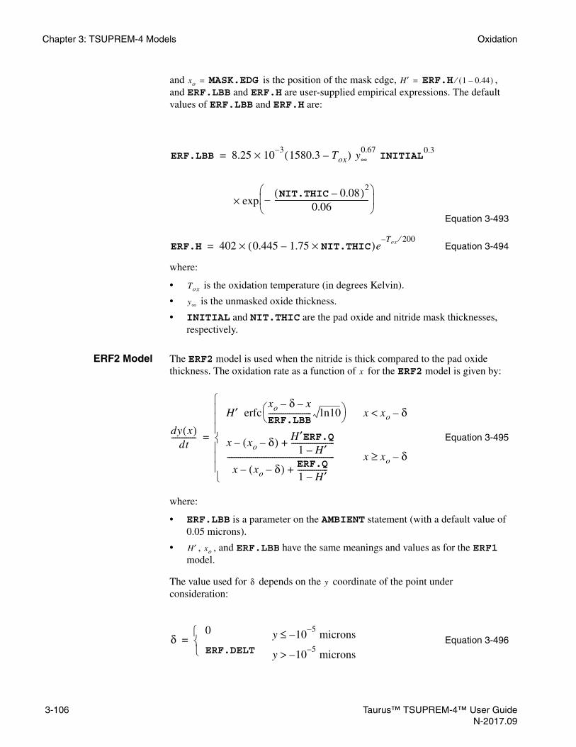
Chapter 3: TSUPREM-4 Models Oxidation

and is the position of the mask edge, , and ERF.LBB and ERF.H are user-supplied empirical expressions. The default values of ERF.LBB and ERF.H are:

Equation 3-493

Equation 3-494

where:

• is the oxidation temperature (in degrees Kelvin).

• is the unmasked oxide thickness.

• INITIAL and NIT.THIC are the pad oxide and nitride mask thicknesses, respectively.

ERF2 Model The ERF2 model is used when the nitride is thick compared to the pad oxide thickness. The oxidation rate as a function of for the ERF2 model is given by:

Equation 3-495

where:

• ERF.LBB is a parameter on the AMBIENT statement (with a default value of 0.05 microns).

• , , and ERF.LBB have the same meanings and values as for the ERF1 model.

The value used for depends on the coordinate of the point under consideration:

Equation 3-496

xo MASK.EDG= H′ ERF.H 1 0.44–( )⁄=

ERF.LBB 8.25 103–

1580.3 Tox–( ) y∞0.67

INITIAL0.3

exp NIT.THIC 0.08–( )2

0.06--------------------------------------------------–

×

×=

ERF.H 402 0.445 1.75 NIT.THIC×–( )eTox 200⁄–

×=

Tox

y∞

x

dy x( )dt

-------------

H′ erfcxo δ– x–

ERF.LBB----------------------- ln10 x xo δ–<

x xo δ–( ) H′ERF.Q1 H′–

-----------------------+–

x xo δ–( ) ERF.Q

1 H′–----------------+–

--------------------------------------------------------- x xo δ–≥

=

H′ xo

δ y

δ0 y 10

5– microns–≤

ERF.DELT y 105– microns–>

=

3-106 Taurus™ TSUPREM-4™ User GuideN-2017.09

Oxidation Chapter 3: TSUPREM-4 Models

where ERF.DELT is a parameter on the AMBIENT statement (with a default value of 0.04 microns). Thus the breakpoint in Equation 3-495 occurs at MASK.EDG when calculating the position of the top surface of the oxide ( microns), but is offset by ERF.DELT when calculating the position of the silicon/oxide interface ( microns).

ERFG Model The ERFG model selects either ERF1 or ERF2 depending on the values of INITIAL, and NIT.THIC. ERF1 is used if

, and ERF2 is used otherwise.

RecommendedUsage

The ERFG models provide a fast, analytical simulation of local oxidation of planar surfaces. The accuracy of this model has not been determined. (Note that these models differ slightly from those proposed by Guillemot et al. Guillemot computes the final oxide shape as a function of the final field oxide thickness, while TSUPREM-4 uses the same equations to calculate the oxide growth rate as a function of the field oxide thickness at each time point in the simulation.)

The ERFG shares all the limitations of the ERFC model. In addition, it places more restrictions on the initial structure and has more parameters that need to be determined. The ERFC model is rarely used in practical simulations.

Numerical Oxidation Models

There are four numerical models of oxidation, VERTICAL, COMPRESS, VISCOUS, and VISCOELA in TSUPREM-4. These models are designed for accurate simulation of arbitrary structures, using the masking layers present in the simulated structure. They work by solving Equations 3-474 through 3-478 directly to obtain the growth rate at each point on the oxide/silicon interface. The models differ in the way in which the oxide flow caused by volume expansion is calculated. This section describes the calculation of the oxide growth rate. VERTICAL Model, p. 3-110, COMPRESS Model, p. 3-110,VISCOUS Model, p. 3-112, and VISCOELA Model, p. 3-114 discuss how the four models simulate the oxide flow.

Oxide GrowthRate

The oxide growth rate is calculated using Equations 3-474 through 3-478. Equations 3-474 gives the flux of oxidant molecules entering the oxide from the ambient gas. The gas-phase mass transfer coefficient is given by:

Equation 3-497

where TRANS.0 and TRANS.E are specified on the AMBIENT statement with the OXIDE and /AMBIENT parameters (see Chapter 4, AMBIENT, p. 4-236). Henry’s law coefficient is specified for each oxidizing species (O2 or H2O) with the HENRY.CO parameter on the AMBIENT statement.

y 105– –≤

y 105– –>

NIT.THIC 2.5≤ INITIAL 0.035μm+×

h

h TRANS.0 exp TRANS.E–

kT---------------------------- ⋅=

H

Taurus™ TSUPREM-4™ User Guide 3-107N-2017.09

Chapter 3: TSUPREM-4 Models Oxidation

Diffusion of oxidant through the oxide is modeled by Equation 3-475. The diffusivity is calculated from the parabolic oxidation rate using Equations 3-480 and 3-481:

Equation 3-498

where is given by:

Equation 3-499

and THETA is a parameter on the AMBIENT statement. The parabolic oxidation rate is given by Equation 3-487 in Analytical Oxidation Models, p. 3-101.

The diffusivity in other materials is given by:

Equation 3-500

where D.0 and D.E are parameters on the AMBIENT statement.

The rate at which the oxidant molecules react with silicon at the oxide/silicon interface is given by Equation 3-476. The reaction rate is derived from Equation 3-480:

Equation 3-501

where it is assumed that . The value of is the linear growth rate given by Equation 3-484 in Analytical Oxidation Models, p. 3-101. For polycrystalline materials, this rate is enhanced by the presence of grain boundaries as described in Dependence of Polysilicon Oxidation Rate on Grain Size, p. 3-186.

ConcentrationDependence

The electron concentration dependence of the linear oxidation rate is given by References [25], [26], and [27]:

Equation 3-502

where:

Equation 3-503

B

D BN1

2C*

---------=

N1

N1THETA for O2

2 THETA× for H2O

=

B

D D.0 exp D.E–kT

-------------- ⋅=

ks

ksBA---

N1

C*

------=

k h« B A⁄

lC

lC1 analytical oxidation models

1 γV CV 1–( )+ numerical oxidation models

=

γV GAMMA.0 exp GAMMA.E–

kT---------------------------- ⋅=

3-108 Taurus™ TSUPREM-4™ User GuideN-2017.09

Oxidation Chapter 3: TSUPREM-4 Models

Equation 3-504

The parameters GAMMA.0 and GAMMA.E are specified in the AMBIENT statement for each of the oxidizing species; is the electron concentration in the silicon at the oxidizing interface. The terms , , and are the normalized intrinsic concentrations of positive, negative, and double negative vacancies, respectively, given by:

Equation 3-505

Equation 3-506

Equation 3-507

Equation 3-508

Equation 3-509

Equation 3-510

Equation 3-511

Equation 3-512

The dependence on carrier concentration is a function of the location along the oxidizing interface, and is only used with the numerical oxidation models. The surface reaction rate depends on the local crystal orientation of the interface, which is derived from the user-specified substrate orientation and rotation.

Thin Regime The thin regime oxidation rate constant in Equation 3-478 is given by Reference [20].

Equation 3-513

CV

1 C + ni

n---- C

_

nni---- C =

nni---- 2

+ + +

1 C + C_

C =+ + +---------------------------------------------------------------------------------=

n

C + C_

C =

C + expE + Ei–

kT-----------------

=

C_

expEi E -–

kT-----------------

=

C = exp2Ei E

_– E = –

kT----------------------------------

=

E + 0.35 eV=

E_

Eg 0.57 eV–=

E = Eg 0.12 eV–=

Ei

Eg

2------ 0.75ln 0.719( )kT eV+=

Eg 1.174.73 10

4–T

2×T 636+

--------------------------------- eV–=

rthin THINOX.0= exp THINOX.E–

kT------------------------------- exp

yeff–

THINOX.L-------------------------- ⋅

Taurus™ TSUPREM-4™ User Guide 3-109N-2017.09

Chapter 3: TSUPREM-4 Models Oxidation

where the parameters THINOX.0, THINOX.E, and THINOX.L are specified in the AMBIENT statement (see Chapter 4, AMBIENT, p. 4-236) for each of the oxidizing species. Different values of THINOX.0, THINOX.E, and THINOX.L can be defined for each of the three available silicon orientations and for polysilicon by specifying the <111>, <110>, <100>, or POLYSILI parameters in the AMBIENT statement. The effective thickness at each point on the oxidizing interface is calculated as the oxide thickness required to produce the observed oxidant concentration in a 1-D solution to the Deal-Grove equations.

Usage The numerical models have no restrictions regarding initial oxide thickness. The value of INITIAL need not correspond to the oxide thickness in the starting structure, but is still used for the thickness of the native oxide to be deposited on bare silicon or polysilicon surfaces prior to oxidation.

VERTICAL Model The VERTICAL model is the simplest of the numerical oxidation models in TSUPREM-4. In this model, the oxide/silicon interface is constrained to move in the +y direction while the expansion of the oxide occurs in the -y direction. The implementation assumes that there is a single active oxide/silicon interface, with the oxide on top. All layers above the interface move with the oxide surface, and all layers below the interface remain fixed. Because the growth is only in the y direction, the growth rate depends only on the orientation of the silicon substrate (and not on the orientation of the interface).

RecommendedUsage

The VERTICAL model is the fastest of the numerical oxidation models. It is useful for uniform oxidation with arbitrary initial oxide thickness (INITIAL need not be set), and for local oxidation when the initial structure is approximately planar. It is not appropriate for fully recessed oxides, trenches, or other nonplanar structures. The VERTICAL model can be used to model silicon-on-insulator structures, provided that only one silicon/oxide interface is being oxidized. There must be no path for oxidant to diffuse to underlying oxide layers. The VERTICAL model does not simulate oxidation of polysilicon.

COMPRESSModel

The COMPRESS model simulates viscous flow of the oxide during oxidation. The movement of the oxide/silicon interface is two dimensional (movement is perpendicular to the interface), and variation of crystal orientation along the interface is taken into account when calculating the oxidation rate. The viscous flow of the oxide is calculated in two dimensions using linear (3-node) finite elements.

The name COMPRESS comes from the fact that a small amount of compressibility must be allowed to ensure that the model remains numerically well-behaved. Because of the simplicity of the model and the small amount of compressibility, the model cannot be used to calculate accurate values of stress, and does not include the effects of stress on the oxidation process.

yeff

3-110 Taurus™ TSUPREM-4™ User GuideN-2017.09

Oxidation Chapter 3: TSUPREM-4 Models

CompressibleViscous Flow

The equations governing oxide flow were derived by Chin, et al. Reference [28]. The oxide flow is described by a creeping-flow equation:

Equation 3-514

where:

• is the shear viscosity of oxide.

• is the local velocity.

• is the hydrostatic pressure.

The incompressibility condition can be written:

Equation 3-515

To solve these equations with the 3-node element, the incompressibility condition is modified to relate the divergence of velocity to the pressure:

Equation 3-516

where , specified by POISS.R on the MATERIAL statement (Chapter 4, MATERIAL, p. 4-265), is a parameter analogous to the Poisson ratio. The viscosity is specified by analogy to an elastic model:

Equation 3-517

where is specified by the YOUNG.M parameter on the MATERIAL statement. Equations 3-514, 3-516, and 3-517 are applied to all materials except single-crystal silicon, which remains fixed.

BoundaryConditions

The stress in the direction normal to a material interface is continuous across the interface, while the stress normal to a free surface is zero. There is no slippage between materials at an interface.

Model Parameters Default values of YOUNG.M and POISS.R are provided for each material, except for aluminum and photoresist, which should not be present in the structure during oxidation; users must provide values for these parameters for user-defined materials that are present in the structure during oxidation with the COMPRESS model.

COMPRESS Model:Recommended

Usage

The COMPRESS model is recommended for simulating the oxidation of general nonplanar structures and structures containing polysilicon when stress calculations are not required. Because it does not include the effects of stress on

μ∇2V ∇P=

μ

V

P

∇ V⋅ 0=

∇ V⋅ 1 2v–

μ--------------- P–=

v

μ E2 1 v+( )--------------------=

E

Taurus™ TSUPREM-4™ User Guide 3-111N-2017.09

Chapter 3: TSUPREM-4 Models Oxidation

the oxidation process, the COMPRESS model should be used only when one or more of the following conditions is satisfied:

• Structure is planar.

• Amount of oxide grown is small.

• Exact details of the shape of the oxide are not critical.

When none of these conditions is satisfied, the VISCOELA or VISCOUS model should be used. The COMPRESS mode is slower than the VERTICAL model and has somewhat larger memory requirements.

VISCOUS Model The VISCOUS model simulates viscous flow of the oxide during oxidation. The movement of the oxide/silicon interface is 2-D (movement is perpendicular to the interface), and variation of crystal orientation along the interface is taken into account when calculating the oxidation rate. The viscous flow of the oxide is calculated in two dimensions using 7-node finite elements, which allow accurate values of stress to be computed Reference [29].

IncompressibleViscous Flow

The equations and boundary conditions governing oxide flow are the same as for the COMPRESS model (Equations 3-514 through 3-517), except that surface tension is included (refer to Surface Tension and Reflow, p. 3-119) and a different set of parameters is used. The viscosity is specified for each material by:

Equation 3-518

where VISC.0 and VISC.E are parameters on the MATERIAL statement (see Chapter 4, MATERIAL, p. 4-265). The parameter , which determines the degree of compressibility, is specified as VISC.X on the MATERIAL statement. The default value of for all materials (except aluminum and photoresist) is 0.499, which produces a negligible amount of compressibility; the user must provide values for these parameters for user-defined materials that are present in the structure during oxidation with the VISCOUS model.

The stresses are calculated from the constitutive equations for each material:

Equation 3-519

Equation 3-520

Equation 3-521

μo VISC.0 exp VISC.E–

kT------------------------ ⋅=

v

v

σxx σyy+μ

12--- v–-----------

∂ux

∂x--------

∂uy

∂y--------+

=

σxx σyy– 2μ∂ux

∂x--------

∂uy

∂y--------–

=

σxy μ∂ux

∂y--------

∂uy

∂x--------+

=

3-112 Taurus™ TSUPREM-4™ User GuideN-2017.09

Oxidation Chapter 3: TSUPREM-4 Models

where and are the and components of velocity, and , , and are the components of the stress tensor. The stresses in a purely viscous model are proportional to the flow velocities, and thus fall to zero when oxidation stops. The stresses reported by TSUPREM-4 after an oxidation step are the values calculated at the end of the step, before the flow is stopped. The stresses calculated by the VISCOUS model replace any stresses that may have been previously calculated using the ST.HISTO model or the STRESS statement.

Stress Dependence When STRESS.D is set true on the AMBIENT statement, the surface reaction rate , diffusivity of oxidant in oxide , and the oxide viscosity are modified to

reflect their dependence on the stresses in the oxide:

Equation 3-522

Equation 3-523

Equation 3-524

where , , and are the stress-dependent reaction rate, diffusivity, and viscosity, respectively, and VR, VT, VD, and VC are parameters on the AMBIENT statement. The exponential in Equation 3-523 is limited for positive arguments (that is, negative values of ) to the value of VDLIM (a parameter on the AMBIENT statement) to prevent unrealistic enhancement of the diffusivity. The surface reaction rate depends both on the stress normal to the interface:

Equation 3-525

and on the stress in the plane perpendicular to the interface:

Equation 3-526

where and are the components of the unit vector normal to the interface. The oxidant diffusivity depends on the hydrostatic pressure defined by:

Equation 3-527

while the oxide viscosity depends on the total shear stress :

Equation 3-528

Newton-Raphson iteration is used to solve the nonlinear equations produced by the stress dependencies. Many iterations are usually required for convergence, and in some cases full convergence is not be obtained. Thus, the time required to

ux uy x y σxx σyy σxy

ks D μ

k′s ksexp σnVR

kT-------------–

exp σtVT

kT------------–

=

D′ D exp pVDkT

---------– =

μ μo

σsVC 2kT⁄sinh σsVC 2kT⁄( )-----------------------------------------=

k′s D′ μ

p

σn σxxnx2 σyyny

22σxynxny+ +( )–=

σt σxxny2 σyynx

22σxynxny–+( )–=

nx ny

p

p 12--- σxx σyy+( )–=

σs

σs14--- σxx σyy–( )2 σxy

2+=

Taurus™ TSUPREM-4™ User Guide 3-113N-2017.09

Chapter 3: TSUPREM-4 Models Oxidation

simulate stress-dependent oxidation may be 20–200 times that required without the stress dependencies.

RecommendedUsage

The VISCOUS model has been made largely obsolete by the VISCOELA model. It is more accurate than the VISCOELA model when the viscosity is much smaller than Young’s modulus, but is much slower when stress dependence is used. It is occasionally useful in verifying the results of the VISCOELA model, but it is often difficult to determine whether the difference between the two models is due to the differences in the physical model or to differences in numerical approach.

VISCOELA Model The VISCOELA model simulates viscoelastic flow of the oxide during oxidation. The movement of the oxide/silicon interface is 2-D (movement is perpendicular to the interface), and variation of crystal orientation along the interface is taken into account when calculating the oxidation rate. The viscoelastic flow of the oxide is calculated in two dimensions by using three-node finite elements, which use numerical techniques that allow approximate values of stress to be computed. The model is similar to that developed by Senez, et al., References [30] and in Appendix A.

Viscoelastic Flow The VISCOELA model adds an elastic component to the equations used by the COMPRESS and VISCOUS models. In one dimension, the stress is related to the strain by:

Equation 3-529

where:

• is the modulus of elasticity in shear.

• is the stress relaxation time ( is the viscosity).

This states that the change in stress is proportional to the change in strain, minus a relaxation term that is proportional to the stress. In three dimensions, the equations are written most simply in terms of volumetric (dilatory) and shear components:

Equation 3-530

where:

Equation 3-531

σε

∂σ∂t------ 2G

∂ε∂t-----

στ---–=

G

τ μ G⁄= μ

∂σv

∂t--------- 3K

∂εv

∂t--------

σv

τv-----–= , τv

μv

K-----=

∂σ′∂t

-------- 2G∂ε′∂t-------

σ′τ′-----–= , τ′ μ

G----=

σv13--- σxx σyy σzz+ +( )≡ and εv

13--- εxx εyy εzz+ +( )≡

3-114 Taurus™ TSUPREM-4™ User GuideN-2017.09

Oxidation Chapter 3: TSUPREM-4 Models

are the volumetric components of the stress and strain, respectively, and:

Equation 3-532

are the shear components.

The strains are defined by:

Equation 3-533

where , , and are the components of the flow displacements. Note that and are zero for the 2-D case analyzed in TSUPREM-4.

The stresses must satisfy the force balance equations:

Equation 3-534

These equations can be combined with Equation 3-530 and solved for the flow velocities. The stress in the direction normal to a material interface is continuous across the interface, while the stress normal to a free surface is zero (unless surface tension is included). (See Surface Tension and Reflow, p. 3-119.) There is no slippage between mat.erials at an interface. The equations are solved in silicon only if ^SKIP.SIL has been specified on the METHOD statement.

Model Parameters The VISCOELA model uses the same elasticity parameters as the COMPRESS model and the same viscosity and stress dependence parameters as the VISCOUS model. The bulk modulus and shear modulus are given by:

Equation 3-535

where and are specified on the MATERIAL statement.

σ′

σxx σv–

σyy σv–

σzz σv–

σxy

≡ and ε′

εxx εv–

εyy εv–

εzz εv–

εxy

≡

εxx

∂ux

∂x--------≡ εyy

∂uy

∂y--------≡ εzz

∂uz

∂y--------≡

εxy12---

∂ux

∂y--------

∂uy

∂x--------+

≡

ux uy uz uz

εzz

∂σxx

∂x-----------

∂σxy

∂y----------- 0=+

∂σyy

∂y-----------

∂σxy

∂x----------- 0=+

K G

KE

3 1 2ν–( )-----------------------= , G

E2 1 ν+( )--------------------=

E YOUNG.M= ν POISS.R=

Taurus™ TSUPREM-4™ User Guide 3-115N-2017.09

Chapter 3: TSUPREM-4 Models Oxidation

The bulk viscosity and shear viscosity are given by:

Equation 3-536

where VISC.0, VISC.E, and are specified on the MATERIAL statement. Note that is normally very slightly less than 0.5, so is much larger than and is much larger than typical oxidation times. Thus the relaxation in volumetric stress is negligible.

Stress Dependence The oxidant diffusivity, interface reaction rate, and material viscosities depend on stress in the same way as in the VISCOUS model except that Von Mises shear stress is used when computing material viscosities and that the user-defined multiplication factors can be applied to diffusivity or surface reaction rate. Stress dependence is enabled by default; it can be disabled by specifying ^STRESS.D on the AMBIENT statement.

Equation 3-537

Equation 3-538

R.FACTOR and D.FACTOR are the expressions of the multiplication factors which can be defined for each oxidant in the AMBIENT statement.

Equation 3-539

where , , and are the stress-dependent reaction rate, diffusivity, and viscosity, respectively, and VR, VT, VD, and VC are parameters on the AMBIENT statement. The exponential in Equation 3-523 is limited for positive arguments (that is, negative values of ) to the value of VDLIM (a parameter on the AMBIENT statement) to prevent unrealistic enhancement of the diffusivity. The surface reaction rate depends both on the stress normal to the interface:

Equation 3-540

and on the stress in the plane perpendicular to the interface:

Equation 3-541

where and are the components of the unit vector normal to the interface. The oxidant diffusivity depends on the hydrostatic pressure defined by:

Equation 3-542

μv μ

μv

2μ 1 νv+( )3 1 2νv–( )--------------------------= , μ VISC.0 exp VISC.E–

kT----------------------- ⋅=

νv VISC.X=

νv μv

K τv

k′s R.FACTOR k⋅ sexp σnVR

kT-------------–

exp σtVT

kT------------–

=

D′ D.FACTOR D⋅ exp pVDkT

---------– =

μ μo

σsVC 2kT⁄sinh σsVC 2kT⁄( )-----------------------------------------=

k′s D′ μ

p

σn σxxnx2 σyyny

22σxynxny+ +( )–=

σt σxxny2 σyynx

22σxynxny–+( )–=

nx ny

p

p 13--- σxx σyy σzz+ +( )–=

3-116 Taurus™ TSUPREM-4™ User GuideN-2017.09

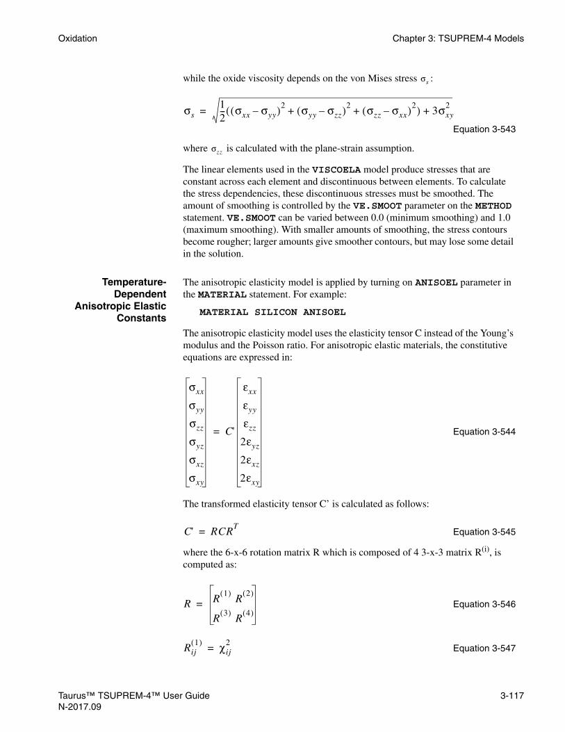
Oxidation Chapter 3: TSUPREM-4 Models

while the oxide viscosity depends on the von Mises stress :

Equation 3-543

where is calculated with the plane-strain assumption.

The linear elements used in the VISCOELA model produce stresses that are constant across each element and discontinuous between elements. To calculate the stress dependencies, these discontinuous stresses must be smoothed. The amount of smoothing is controlled by the VE.SMOOT parameter on the METHOD statement. VE.SMOOT can be varied between 0.0 (minimum smoothing) and 1.0 (maximum smoothing). With smaller amounts of smoothing, the stress contours become rougher; larger amounts give smoother contours, but may lose some detail in the solution.

Temperature-Dependent

Anisotropic ElasticConstants

The anisotropic elasticity model is applied by turning on ANISOEL parameter in the MATERIAL statement. For example:

MATERIAL SILICON ANISOEL

The anisotropic elasticity model uses the elasticity tensor C instead of the Young’s modulus and the Poisson ratio. For anisotropic elastic materials, the constitutive equations are expressed in:

Equation 3-544

The transformed elasticity tensor C’ is calculated as follows:

Equation 3-545

where the 6-x-6 rotation matrix R which is composed of 4 3-x-3 matrix R(i), is computed as:

Equation 3-546

Equation 3-547

σs

σs12--- σxx σyy–( )2 σyy σzz–( )2 σzz σxx–( )2

+ +( ) 3σxy2

+=

σzz

σxx

σyy

σzz

σyz

σxz

σxy

C'

εxx

εyy

εzz

2εyz

2εxz

2εxy

=

C' RCRT

=

R R1( )

R2( )

R3( )

R4( )

=

Rij1( ) χij

2=

Taurus™ TSUPREM-4™ User Guide 3-117N-2017.09

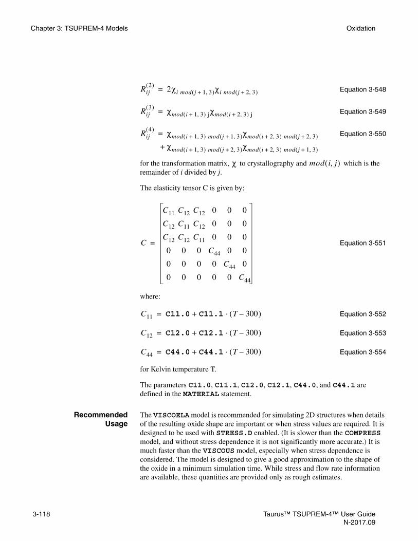
Chapter 3: TSUPREM-4 Models Oxidation

3-118

Equation 3-548

Equation 3-549

Equation 3-550

for the transformation matrix, to crystallography and which is the remainder of i divided by j.

The elasticity tensor C is given by:

Equation 3-551

where:

Equation 3-552

Equation 3-553

Equation 3-554

for Kelvin temperature T.

The parameters C11.0, C11.1, C12.0, C12.1, C44.0, and C44.1 are defined in the MATERIAL statement.

RecommendedUsage

The VISCOELA model is recommended for simulating 2D structures when details of the resulting oxide shape are important or when stress values are required. It is designed to be used with STRESS.D enabled. (It is slower than the COMPRESS model, and without stress dependence it is not significantly more accurate.) It is much faster than the VISCOUS model, especially when stress dependence is considered. The model is designed to give a good approximation to the shape of the oxide in a minimum simulation time. While stress and flow rate information are available, these quantities are provided only as rough estimates.

Rij2( )

2χi mod j 1 3,+( )χi mod j 2 3,+( )=

Rij3( ) χmod i 1 3,+( ) jχmod i 2 3,+( ) j=

Rij4( ) χmod i 1 3,+( ) mod j 1 3,+( )χmod i 2 3,+( ) mod j 2 3,+( )

χmod i 1 3,+( ) mod j 2 3,+( )χmod i 2 3,+( ) mod j 1 3,+( )+

=

χ mod i j,( )

C

C11 C12 C12 0 0 0

C12 C11 C12 0 0 0

C12 C12 C11 0 0 0

0 0 0 C44 0 0

0 0 0 0 C44 0

0 0 0 0 0 C44

=

C11 C11.0 C11.1 T 300–( )⋅+=

C12 C12.0 C12.1 T 300–( )⋅+=

C44 C44.0 C44.1 T 300–( )⋅+=

Taurus™ TSUPREM-4™ User GuideN-2017.09

Oxidation Chapter 3: TSUPREM-4 Models

The VISCOELA model must be used when comprehensive stress history modeling (using ST.HISTO) is required; see Stress History Model, p. 3-130. When ST.HISTO is used with the VISCOELA model, intrinsic and thermal mismatch stresses are included in the oxidation model and the stress model is enabled during inert anneals to model relaxation of stresses in the structure.

AnisotropicStress-

DependentReaction

Due to crystal anisotropy, reactions across silicon-oxide interface take place at different rates, and the dependence of the reaction rates on local stress is a function of the local crystal orientation. This anisotropic stress dependence of reaction rate often leads to the formation of distinctive <111> facets at the silicon-oxide interface near the STI bottom corners. When ST.R.ANIis set true on the AMBIENT statement, the surface reaction rate in Equation 3-522 is computed using crystal orientation dependent parameters VR, and VT, where VR is extracted from normal activation volumes in 100, 110 and 111 crystal directions, VR100, VR110, and VR111 respectively; and VT is extracted from tangential activation volumes in 100, 110 and 111 crystal directions, VT100, VT110, and VT111 respectively. The individual activation volumes in normal and tangential directions across the reaction interface are parameters on the AMBIENT statement. It is applicable only to the VISCOUS and VISCOELA models.

Strength-LimitedStress

The strength limit model can be used to prevent unphysical large stress levels during the stress simulation. Once the model is turned on, the absolute stress values for each stress component are bounded within the strength limit. The ST.LIMIT parameter in the METHOD command can be used to turn on the model. The default setting for the parameter is off and the default strength limit is taken as 1/20 of the Young’s modulus. The STRENGTH parameter can be reset by using the MATERIAL command. It is applicable only to the VISCOUS and VISCOELA models.

Polysilicon Oxidation

The oxidation of polysilicon is treated using the models for the oxidation of silicon. Only the COMPRESS, VISCOUS, and VISCOELA models allow oxidation of polysilicon. Values of THINOX.0, THINOX.E, THINOX.L, L.LIN.0, L.LIN.E, H.LIN.0, and H.LIN.E may be defined for polysilicon by specifying the POLYSILI parameter on the AMBIENT statement. The ratio of polysilicon thickness consumed to oxide thickness grown can be defined with the ALPHA parameter on the AMBIENT statement.

Surface Tension and Reflow

The VISCOUS and VISCOELA models include the effects of surface tension. The surface tension is modeled as a tensile force along the surface of magnitude specified by the SURF.TEN parameter on the MATERIAL statement. On planar surfaces, the forces on either side of any point of the surface cancel, giving no net force. But on curved surfaces there is a net force in the direction of the curvature

k′s

Taurus™ TSUPREM-4™ User Guide 3-119N-2017.09

Chapter 3: TSUPREM-4 Models Oxidation

with magnitude inversely proportional to the radius of curvature. The resulting force tends to round off corners and smooth irregularities in the surface. With appropriate values of SURF.TEN and material viscosities, the surface tension model can be used to simulate reflow processes.

The surface tension model is active during oxidation with the VISCOUS and VISCOELA model and whenever stress history modeling is active (that is, when both VISCOELA and ST.HISTO are used).

N2O Oxidation

In N2O oxidation or oxynitridation, nitrogens are trapped at Si/SiO2 interfaces so that the number of oxidizing sites, for this reason the oxidation rate is reduced. N2O oxidation is specified by the N2O parameter in the DIFFUSION statement.

Nitrogen Trapand Generation

It is assumed that N2O oxidants reach to Si/SiO2 interfaces then break up there so that nitrogens are generated. Some of nitrogen are trapped at the interfaces. The trapping flux of nitrogen is described with the interface trap model by ignoring the detrapping flux.

Equation 3-555

where h is the trapping rate, Ci is the nitrogen concentration at the interface. σN and σmax are the trapped density and the maximum trap density, respectively. The coefficients h and σmax are specified in the IMPURITY statement (See Segregation Flux, p. 3-63). The total nitrogen flux at interfaces is the sum of the trapping flux into interfaces and the 2-phase segregation flux into adjacent materials. The generation rate of nitrogen is dependent on the boundary velocity and is given by:

Equation 3-556

Equation 3-557

The N.G.0, N.G.E, N.V.0, N.V.E, N.GPOW.0, and N.GPOW.E are specified in the AMBIENT statement.

Note:N2O oxidation invokes the interface trap model for nitrogen regardless of the specification of the ITRAP parameter in the METHOD statement.

Ftrap hCi 1σN

σmax-----------–

ni=

G N.G.0N.G.E

kT----------------–

vv

N.V.0N.V.E

kT----------------–

exp---------------------------------------------------

gpow·

exp=

gpow N.GPOW.0N.GPOW.E

kT--------------------------–

exp=

3-120 Taurus™ TSUPREM-4™ User GuideN-2017.09

Oxidation Chapter 3: TSUPREM-4 Models

Surface ReactionRate

Since the surface reaction rate is proportional to the number of available oxidizing sites, the rate of oxidant consumption at the oxidizing interface is given by:

Equation 3-558

where:

• ks is the surface reaction rate.

• Ci is the oxidant concentration at the interface.

• σN is the nitrogen density trapped at the interface.

• Different values of N.0 and N.E can be defined for each of the three available silicon orientations and for polysilicon by specifying the <111>, <110>, <100>, or POLYSILI parameters in the AMBIENT statement.

Thin OxidationRate

For the thin oxidation regime, the thin oxidation rate is given by:

Equation 3-559

Different values of N.THIN.0 and N.THIN.E can be defined for each of the three available silicon orientations and for polysilicon by specifying the <111>, <110>, <100>, or POLYSILI parameters in the AMBIENT statement.

Boron Diffusion Enhancement in Oxides

Ultrathin gate oxides allow easier dopant penetration between polysilicon and bulk silicon. Boron penetrates more easily than most other dopants because it has a larger diffusivity than the others do. A nonstoichiometric layer rich in peroxy-linkage-defect forms when oxide is grown on top of the silicon Reference [31]. Dopant diffusion is enhanced in thinner oxides because of the greater ratio of nonstoichiometric layer thickness to the total oxide thickness. Also fluorine increases the number of peroxy-linkage-defects and thus enhances dopant diffusion.

F ksCi 1σN

N.0N.EkT

----------– exp

----------------------------------------–

ni=

rthin THINOX.0THINOX.E

kT----------------------------–

y– eff

THINOX.L----------------------------

1σN

N.THIN.0N.THIN.E

kT----------------------------–

exp

----------------------------------------------------------------------------–

×

expexp=

Taurus™ TSUPREM-4™ User Guide 3-121N-2017.09

Chapter 3: TSUPREM-4 Models Oxidation

DiffusionEnhancement in

Thin Oxides

It is assumed that the formation of silicon-oxide (SiO) due to the reaction between oxygen and silicon atom increases the number of peroxy-linkage-defects. The interstitial segregation at silicon/oxide interfaces introduces silicon atoms into the oxide. The SiO is assumed to be immobile and to react with oxygen to produce SiO2 to rarely dissolve into SiO and O. The volume expansion due to this SiO2 formation in bulk is assumed to be negligible. The diffusivity of impurities depends on the distribution of SiO.

Equation 3-560

Equation 3-561

Equation 3-562

Equation 3-563

, and are the concentrations of silicon atom, SiO in oxide, and interstitial in silicon, respectively. The diffusivity of silicon atom in oxide is set to Reference [32]. is the segregation value of interstitial at the interface between silicon and oxide. Its value is set to

corresponding to the value of Agarwal’s work Reference [32]. and are the bulk reaction rates of silicon atom and SiO with oxygen, respectively. is the reaction rate of silicon atom with oxygen at oxide surfaces.

The diffusion enhancement in oxide is described as follows:

Equation 3-564

is a diffusivity in pure thick oxides. is the temperature-dependent factors for the diffusion-enhancement due to SiO. is the constant for normalization ( /cm3).

The activation energy of is set to -0.28 eV Reference [31]. The experimental data for calibration were taken from Reference [33]. It is assumed that has the same value as to avoid the redundancy due to the lack of measured data. The new impurity names for silicon atom and SiO are given by IOX and SIO, respectively.

IMPURITY MODEL=DEOX IMP=IOX NEW C.INIT=1E5IMPURITY MODEL=DEOX IMP=SIO NEW C.INIT=1E5METHOD IMP=IOX PART REL.ERR=0.01 ABS.ERR=1E9METHOD IMP=SIO NONE REL.ERR=0.01 ABS.ERR=1E9

∂CSi

∂t----------- ∇ DSi∇CSi–

kSiCSi CO2–⋅–=

∂CSiO

∂t-------------- kSiCSi CO2

kSiOCSiO CO2–=

FSi hSi CSi mI–( ) at silicon/oxide interfaces=

FSi kiCSi at oxide surfaces=

CSi CSiO I

DSi

13.0 4.5eV kT⁄–( )exp m

2.9 105–× 2.19eV kT⁄( )exp mCI

*

kSi kSiO

ki

D Do 1 fSiO

CSiO

CSiO2

-------------+ =

D0 fSiO

CSiO2

2.2 1022×

fSiO

KSiO

KSi

3-122 Taurus™ TSUPREM-4™ User GuideN-2017.09

Oxidation Chapter 3: TSUPREM-4 Models

TaurN-20

The diffusivities of silicon atom and boron in oxide is given by:

IMPURITY IMP=IOX MAT=OXIDE DIX.0=13.0 +DIX.E=4.5 CM.SEC

IMPURITY D.MODEL=DEOX IMP=BORON MAT=OXIDE +DI.FAC=1+4.55e-22*exp(0.28/kt)*SIO

The bulk reactions are given by:

REACTION MODEL=DEOX +NAME=KbIOXnO MAT.BULK=OXIDE +IMP.L=IOX /IMP.L=O2 IMP.R=SIO +EI.L=1.0 /EI.L=0.5 EI.R=1.0 +NI.L=1.0 /NI.L=0.0 NI.R=1.0 +RATE.0=7.673E6 RATE.E=4.0 EQUIL.0=0.0

REACTION MODEL=DEOX +NAME=KbSiOnO MAT.BULK=OXIDE +IMP.L=SiO /IMP.L=O2 +EI.L=1.0 /EI.L=0.5 +NI.L=1.0 /NI.L=0.0 +RATE.0=7.673E6 RATE.E=4.0 EQUIL.0=0.0

The segregation flux of interstitial is given by:

REACTION MODEL=DEOX +NAME=ISEG +/MAT.L=OXIDE MAT.R=SILICON +/IMP.L=IOX IMP.R=INTERST +RATE.0=0.01 RATE.E=0.0 +EQUIL.0=2.9E-5 EQUIL.E=-2.19

The surface reaction rate of silicon atom is given by:

REACTION MODEL=DEOX +NAME=KiIOX +/MAT.L=OXIDE MAT.R=AMBIENT +/IMP.L=IOX IMP.R=O2 +/EI.L=1.0 EI.R=1.0 +/NI.L=1.0 NI.R=0.0 +RATE.0=8.67E7 RATE.E=4.0 EQUIL.0=0.0

Since the model DEOX is initially disabled in s4init file, it needs to be activated to use the model by:

METHOD MODEL=DEOX ENABLE

The SiO distribution is believed to be mostly concentrated near the Si/SiO2 interface and thus the dense grid structure is needed near the interface. Usually it is believed that the native oxide thickness must be thinner than the default value 20 angstroms.

METHOD DY.OXIDE=0.0005AMBIENT INITIAL=0.0005

us™ TSUPREM-4™ User Guide 3-12317.09

Chapter 3: TSUPREM-4 Models Silicide Models

Note:This model applies only to dry oxidation. The accuracy of this model is not verified for the oxidation on low oxygen pressure.

DiffusionEnhancement

Due to Fluorine

Fluorine enhances the boron diffusion in oxides. For the diffusion model of fluorine, fluorine is assumed to be electrically neutral. The diffusion enhancement due to fluorine is added to Equation 3-564.

Equation 3-565

where is an equilibrium constant and is a fluorine concentration. and the diffusivities and segregation values of fluorine were extracted by fitting the published data Reference [34].

IMPURITY D.MODEL=DEOX IMP=BORON MAT=OXIDE +DI.FAC=1+4.55e-22*exp(0.28/kt)*SIO+2.23e-20*Fluorine

To consider the fluorine effect, the model FLUORINE as well as the model DEOX must be activated as follows:

METHOD MODEL=DEOX ENALEMETHOD MODEL=FLUORINE ENABLE

If the model FLUORINE is enabled while the model DEOX is disabled, the diffusion enhancement of boron due to fluorine is ignored even though the diffusion equation for fluorine is solved.

Note:In s4init, MODEL=FLUORINE is enabled from version A-2008.09. Thus, TSUPREM-4 simulates the fluorine diffusion when fluorine atoms are present in the structure. However, BF2 implantation does not introduce fluorine atoms by default. To add fluorine atoms by BF2 implants, either II.MOLEC in the METHOD statement or MOLECULE in the BF2 IMPLANT statement must be turned on.

Silicide ModelsTSUPREM-4 allows you to define models for new materials and reactions. This ability has been used to define models for the growth of titanium and tungsten silicides. The following sections describe the kinetics of TiSi2 growth, the specification of the model and parameters, and suggestions for how you can model other silicides.

D Do 1 fSiO

CSiO

CSiO2

------------- fF

CF

CSiO2

-------------+ + =

fF CF fF

3-124 Taurus™ TSUPREM-4™ User GuideN-2017.09

Silicide Models Chapter 3: TSUPREM-4 Models

TiSi2 Growth Kinetics

Titanium silicide is assumed to form when silicon atoms react in the silicide with titanium at the TiSi2/Ti interface. The consumption of silicon and titanium lead to deformation of the material layers in the structure. Note that while the discussion that follows describes the growth of TiSi2 on silicon, it also applies to growth of TiSi2 on polycrystalline silicon.

Reaction at TiSi2/Si Interface

At the TiSi2/Si interface you have the reaction:

Equation 3-566

Thus silicon (on the Si side of the interface) reacts to form silicon atoms (on the TiSi2 side of the interface) plus some number of vacancies (on the Si side of the interface). The reaction is reversible, allowing the reformation of silicon (if silicon is released by nitridation of TiSi2, for example). The forward rate of this reaction depends only on temperature, while the reverse rate is also proportional to the concentration of diffusing silicon atoms in the TiSi2. For each silicon atom removed from the silicon side of the interface, the volume of silicon is reduced by:

Equation 3-567

where MOL.WT and DENSITY are the molecular weight and density, respectively, of silicon, as specified on the MATERIAL statement.

Diffusion ofSilicon

Silicon is transported across the TiSi2 layer by simple diffusion:

Equation 3-568

where is the concentration of diffusion silicon atoms and is their diffusivity.

Reaction at TiSi2/Si Interface

At the TiSi2/Ti interface you have the reaction:

Equation 3-569

This reaction is assumed to be irreversible. The forward reaction rate is proportional to the concentration of diffusing silicon at the TiSi2 side of the interface. The volumes of Ti and TiSi2 change according to Equation 3-567.

OxygenDependence

The silicidation process may be influenced by the presence of oxygen in the silicide[35]. This oxygen is assumed to enter the silicide at interfaces with silicon dioxide and diffuse in the silicide according to Fick’s law. The oxygen retards the reaction of silicon atoms at the silicide/silicon and silicide/metal interfaces and the

Si(Si) →← Si(TiSi2) + aV(Si)

a

ΔV MOL.WT

6.022 1023× DENSITY×------------------------------------------------------------=

∂C∂t------- ∇ D∇C–

⋅–=

C D

2Si TiSi2( ) Ti Ti( )+ →← TiSi2 TiSi2( )

Taurus™ TSUPREM-4™ User Guide 3-125N-2017.09

Chapter 3: TSUPREM-4 Models Silicide Models

diffusion of silicon in the silicide. The retardation factor is assumed to be of the form , where is the oxygen concentration in the silicide and is a critical oxygen concentration for the reduction.

Initialization The TiSi2 growth model is initialized by inserting a thin layer of titanium silicide between layers of titanium and silicon (or polysilicon) wherever they come into contact. This layer is added automatically as needed when titanium is deposited.

Material Flow Consumption of silicon and titanium and growth of TiSi2 cause distortion of the layers making up the structure. The flow of material caused by silicidation is calculated using the VERTICAL, COMPRESS, or VISCOELA growth models described in VERTICAL Model, p. 3-110, the COMPRESS Model, p. 3-110, and the VISCOELA Model, p. 3-114; silicide growth occurs only if one of these models has been specified.

Impurities and Point Defects

Impurities in silicides are modeled in the same way as in other nonsemiconductor materials. Transport within a silicide is governed by simple diffusion (that is, no electric field effects). Segregation at material interfaces is as described in Segregation of Impurities, p. 3-63.

Point defects can participate in reactions at interfaces with silicon. The current titanium silicide model specifies the generation of vacancies by the consumption of silicon (Equation 3-566). The reaction rate has not yet been adequately calibrated to experimental data, however; it is suggested that the PD.FERMI model be used for silicide growth processes.

Specifying Silicide Models and Parameters

The specification of the titanium silicide model requires the following:

• The new materials (titanium and TiSi2 in this case) must be defined.

• Any diffusing species that participates in the growth reactions must be defined.

• The growth reactions themselves (one at each interface) must be defined.

• The deposition of initial layers (for example, the initial TiSi2 layer between titanium and silicon) must be specified.

• The diffusion and segregations of impurities in the new materials and at interfaces must be specified.

All of these are accomplished with TSUPREM-4 input statements. Thus no new code is required to implement new silicide models.

1 min CO COcrit⁄ 1,( )– COCOcrit

3-126 Taurus™ TSUPREM-4™ User GuideN-2017.09

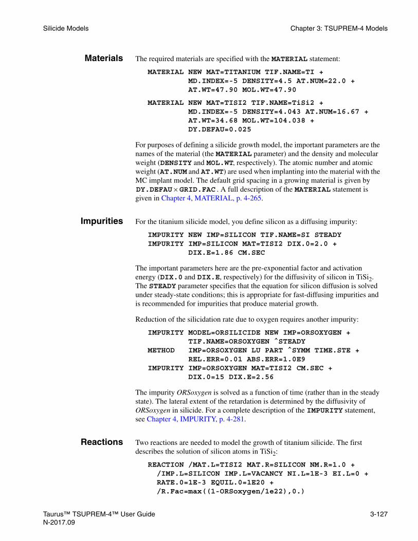
Silicide Models Chapter 3: TSUPREM-4 Models

Materials The required materials are specified with the MATERIAL statement:

MATERIAL NEW MAT=TITANIUM TIF.NAME=TI +MD.INDEX=-5 DENSITY=4.5 AT.NUM=22.0 +AT.WT=47.90 MOL.WT=47.90

MATERIAL NEW MAT=TISI2 TIF.NAME=TiSi2 +MD.INDEX=-5 DENSITY=4.043 AT.NUM=16.67 +AT.WT=34.68 MOL.WT=104.038 +DY.DEFAU=0.025

For purposes of defining a silicide growth model, the important parameters are the names of the material (the MATERIAL parameter) and the density and molecular weight (DENSITY and MOL.WT, respectively). The atomic number and atomic weight (AT.NUM and AT.WT) are used when implanting into the material with the MC implant model. The default grid spacing in a growing material is given by

. A full description of the MATERIAL statement is given in Chapter 4, MATERIAL, p. 4-265.

Impurities For the titanium silicide model, you define silicon as a diffusing impurity:

IMPURITY NEW IMP=SILICON TIF.NAME=SI STEADYIMPURITY IMP=SILICON MAT=TISI2 DIX.0=2.0 +

DIX.E=1.86 CM.SEC

The important parameters here are the pre-exponential factor and activation energy (DIX.0 and DIX.E, respectively) for the diffusivity of silicon in TiSi2. The STEADY parameter specifies that the equation for silicon diffusion is solved under steady-state conditions; this is appropriate for fast-diffusing impurities and is recommended for impurities that produce material growth.

Reduction of the silicidation rate due to oxygen requires another impurity:

IMPURITY MODEL=ORSILICIDE NEW IMP=ORSOXYGEN +TIF.NAME=ORSOXYGEN ^STEADY

METHOD IMP=ORSOXYGEN LU PART ^SYMM TIME.STE +REL.ERR=0.01 ABS.ERR=1.0E9

IMPURITY IMP=ORSOXYGEN MAT=TISI2 CM.SEC +DIX.0=15 DIX.E=2.56

The impurity ORSoxygen is solved as a function of time (rather than in the steady state). The lateral extent of the retardation is determined by the diffusivity of ORSoxygen in silicide. For a complete description of the IMPURITY statement, see Chapter 4, IMPURITY, p. 4-281.

Reactions Two reactions are needed to model the growth of titanium silicide. The first describes the solution of silicon atoms in TiSi2:

REACTION /MAT.L=TISI2 MAT.R=SILICON NM.R=1.0 +/IMP.L=SILICON IMP.L=VACANCY NI.L=1E-3 EI.L=0 +RATE.0=1E-3 EQUIL.0=1E20 +/R.Fac=max((1-ORSoxygen/1e22),0.)

DY.DEFAU GRID.FAC×

Taurus™ TSUPREM-4™ User Guide 3-127N-2017.09

Chapter 3: TSUPREM-4 Models Silicide Models

This statement implements the reverse of the reaction of Equation 3-566:

Equation 3-570

Parameters ending in “.L” denote reactants (silicon atoms in TiSi2 and vacancies in silicon) while parameters ending in “.R” denote products (bulk silicon). Parameters can also be classified by which side of the material interface they are associated with. In this case, the vacancies are on the silicon side of the interface (no “/” in the parameter name), while silicon (as an impurity) is on the TiSi2 side of the interface (with “/” in the parameter name).

By default, one molecule of each impurity and no molecules of each material participate in the reaction. These defaults have been overridden for silicon (NM.R=1.0 implies that one silicon atom participates) and for vacancies (NI.L=1e-3 implies that one vacancy is generated for each 1000 reactions). The forward reaction rate in this case is given by:

Equation 3-571

where and denote the vacancy and silicon concentrations, respectively. EI.L=0 has been specified, so there is no dependency on the vacancy concentration; /EI.L defaults to 1.0. /R.FAC models the reduction in the reaction rate caused by oxygen in the silicide. The equilibrium concentration of reactant impurities to product impurities is given by:

Equation 3-572

Note:There are no product impurities in this case. The equilibrium concentration of silicon diffusing in TiSi2 has been specified as 1e20.

For a complete description of the REACTION statement, see Chapter 4, REACTION, p. 4-308.

The reaction at the interface between TiSi2 and polysilicon is the same as at silicon interfaces except that no vacancies are involved:

REACTION /MAT.L=TISI2 MAT.R=POLY NM.R=1.0 +/IMP.L=SILICON RATE.0=1E-3 EQUIL.0=1E20/R.Fac=max((1-ORSoxygen/1e22),0.)

The reaction at the Ti/TiSi2 interface is specified by:

REACTION /MAT.L=TITANIUM /NM.L=0.5 MAT.R=TISI2 +NM.R=0.5 IMP.L=SILICON RATE.0=104 RATE.E=1.0 +EQUIL.0=1.0 R.Fac=max((1-ORSoxygen/1e22),0.)

Si TiSi2( ) 103–V Si( )+ →← Si Si( )

Rf /R.FAC RATE.0⋅ exp RATE.E–

kT------------------------ V[ ]EI.L Si[ ]/EI.L=

V[ ] Si[ ]

V[ ]EI.L Si[ ]/EI.L EQUIL.0 exp EQUIL.E–

kT---------------------------- =

3-128 Taurus™ TSUPREM-4™ User GuideN-2017.09

Silicide Models Chapter 3: TSUPREM-4 Models

This corresponds directly with Equation 3-569 except that you have divided the quantities of all reactants by two. The forward reaction rate is proportional to the silicon concentration at the Ti/TiSi2 interface. The equilibrium ratio of reactant impurities to product impurities (=[Si]) has been set to 1.0, a very small value. The reduction in the rate due to oxygen is specified by R.FAC rather than /R.FAC because in this reaction the silicide is specified as MAT.R (instead of /MAT.L).

The initial TiSi2 layers to be deposited between titanium layers and exposed silicon and poly silicon layers are also specified with REACTION statements:

REACTION MAT=TITANIUM /MAT=SILICON +MAT.NEW=TISI2 THICK=0.002

REACTION MAT=TITANIUM /MAT=POLY +MAT.NEW=TISI2 THICK=0.002

These specify that 0.002 microns of TiSi2 should be deposited on silicon or polysilicon before depositing titanium.

Dopants Diffusion and segregation of impurities in silicides are specified in the usual way:

BORON MAT=TISI2 CM.SEC DIX.0=6.0E-7 DIX.E=2.0BORON SILICON /MAT=TISI2 SEG.0=0.3 +

TRANS.0=1E-6 TRANS.E=2.0BORON MAT=POLY /MAT=TISI2 SEG.0=0.3 +

TRANS.0=1E-6 TRANS.E=2.0

The MATERIAL and /MATERIA parameters must be used when specifying new material names; they are optional when specifying old built-in materials. These parameters could also be specified with the IMPURITY statement:

IMPURITY IMP=BORON MAT=TISI2 CM.SEC +DIX.0=6.0E-7 DIX.E=2.0

IMPURITY IMP=BORON MAT=SILICON /MAT=TISI2 +SEG.0=0.3 TRANS.0=1E-6 TRANS.E=2.0

Tungsten, Cobalt, and Nickel Silicide Models

The tungsten, cobalt, and nickel silicide models are identical in form to the titanium silicide model. The parameters of the models are different, however, reflecting the differences between the materials (see References [36] to [42] for the tungsten silicide model and References [43] to [47] for the cobalt silicide model). The names of the relevant materials are tungsten and WSi2 for tungsten silicide, cobalt and CoSi2 for cobalt silicide, and nickel and NiSi2 for nickel silicide.

Taurus™ TSUPREM-4™ User Guide 3-129N-2017.09

Chapter 3: TSUPREM-4 Models Stress Models

Other Silicides

Models for other silicides can be defined following the example given above for titanium silicide. The diffusing impurity in the silicide can be metal or silicon or both.

Stress ModelsTSUPREM-4 has several models for calculating the stresses produced during the fabrication model. The most complete is the stress history (ST.HISTO) model. Older and more limited capabilities are provided by the STRESS statement and the VISCOUS oxidation model.

Stress History Model

A number of physical phenomena give rise to stress in a structure during fabrication. These include volume changes during oxidation, thermal mismatch between materials, intrinsic strain in deposited layers, and surface tension. These phenomena are simulated by the stress history (ST.HISTO) model in TSUPREM-4.

Thermal Stress Model Equations

The effect of thermal expansion during temperature ramping is modeled by adding an additional term to Equation 3-530 for the volumetric stress:

Equation 3-573

where LCTE is the linear coefficient of thermal expansion specified on the MATERIAL statement and is the temperature.

BoundaryConditions

The boundary conditions assume that the thermal expansion is dominated by a thick silicon substrate with equivalent conditions on the front and back surfaces (so there is no curvature of the wafer). Thermal expansion of the substrate produces a constant strain in the direction. The displacement in the x direction at vertical reflecting boundaries and in silicon when SKIP.SIL is set is proportional to x, ux = xLCTEΔT, while the displacement in the y direction at horizontal reflecting boundaries and in silicon when SKIP.SIL is set is proportional to y, uy = yLCTEΔT. The value of LCTE for silicon is used for these boundary conditions.When solving thermal stress equations with above boundary conditions, no thermal stresses are generated in the thick silicon substrate. The expanded substrate is then used as a reference to calculate the relative thermal expansions for the layer structures above the substrate. (When

∂σv∂t

--------- 3K∂εv∂t

-------- LCTEdTdt------–

σvτv------–=

T

εzz LCTE TΔ= z

3-130 Taurus™ TSUPREM-4™ User GuideN-2017.09

Stress Models Chapter 3: TSUPREM-4 Models

saving strain components to results files, only the mechanical deformation strains are saved.}

Surface tension acts on the surface of the structure; see Surface Tension and Reflow, p. 3-119 for details.

Initial Conditions The final stress from one high-temperature processing step is used as the starting stress for the next; if the temperature changes between the end of one step and the start of the next, a very short ramping step is inserted automatically by the program to compute the change in stress caused by the change in temperature. The stress is set to zero at the first temperature specified after structure initialization; this temperature may be specified as part of a high-temperature processing step (that is, DIFFUSION, DEPOSITION, or EPITAXY) or on a SELECT or SAVEFILE statement. The stresses may be modified during deposition and etching, as described below. The STRESS statement and oxidation with the VISCOUS model compute new stresses, ignoring and replacing previously calculated values.

Intrinsic Stressin Deposited

Layers

The intrinsic stress in deposited layers can be specified for each material with the INTRIN.S parameter on the MATERIAL statement. This intrinsic stress is included whenever stress history modeling is enabled. Each deposition step is followed by a stress relaxation calculation to determine the stresses in the structure following the deposition. The model includes the effects of surface tension; the stress is only calculated when ST.HISTO and VISCOELA models are active.

Note:The interpretation of the INTRIN.S parameter by the stress history model is different from that used by the STRESS statement (obsolete). Both work by placing an initial stress in the deposited layer and then allowing the layer to relax to conform to the boundary conditions (for example, zero stress normal to free surfaces). The STRESS statement uses INTRIN.S as the initial stress, while the stress history model uses an initial stress that gives INTRIN.S as the x (and z) component of stress in a uniform, planar layer after relaxation. Table 3-1 summarizes the difference. For the ST.HISTO model to generate the same results as the STRESS statement, you must multiply INTRIN.S by

, where is the value of POISS.R.1 2ν–( ) 1 ν–( )⁄ ν

Taurus™ TSUPREM-4™ User Guide 3-131N-2017.09

Chapter 3: TSUPREM-4 Models Stress Models

Effect of Etchingand Depositional

Stress

When stressed material is removed or deposited from a structure, the balance of forces acting on the remaining material changes, as do the stresses in the remaining structure. Thus, each etching or deposition step is followed by a stress relaxation calculation to determine the stresses in the structure after the etch. The model includes the effects of surface tension; the stress is only calculated when the ST.HISTO and VISCOELA models are active.

Using the StressHistory Model

The stress history in a structure is simulated when the following conditions are satisfied:

• Stress history simulation has been enabled by the ST.HISTO parameter on the METHOD statement:

METHOD ST.HISTO

• The VISCOELA oxidation model has been selected

Stresses in silicon are simulated only if ^SKIP.SIL has been specified on the METHOD statement. Thermal mismatch stresses are simulated whenever temperature ramping is specified on the DIFFUSION statement. Intrinsic stresses are included during deposition whenever INTRIN.S for the deposited material is nonzero. Surface tension is included whenever SURF.TEN for an exposed material is nonzero.

Limitations The thermal stress model has the following limitations:

• The model assumes that thermal expansion is dominated by a thick silicon substrate with equivalent conditions on the front and back sides of the wafer (that is, no bending of the wafer). Although thermal expansions are assumed to take place isotropically, which introduce a thermal strain in z direction, the modeling of mechanical deformation is based on plane strain conditions.

• The model is active only when the VISCOELA oxidation model is active. Stresses in silicon are calculated only if ^SKIP.SIL has been specified. The stress history is lost and replaced with newly calculated stresses by the STRESS statement and during oxidation with the VISCOUS model.

Table 3-1 Model Comparisons After Relaxation

Model Initial After Relaxation

ST.HISTO

STRESS (OBSOLETE)

σxx σyy σzz INTRIN.S1 ν–

1 2ν–---------------= = = σyy 0

σxx

,σzz INTRIN.S

== =

σxx σyy σzz INTRIN.S= = = σyy 0

σxx

,

σzz INTRIN.S1 2ν–1 ν–

---------------

=

= =

3-132 Taurus™ TSUPREM-4™ User GuideN-2017.09

Stress Models Chapter 3: TSUPREM-4 Models

• While the thermal mismatch model works down to room temperature, the diffusion models do not. At temperatures below about 50°C they may produce arithmetic exceptions or cause the program to hang; below about 600°C they may produce inaccurate results.

• The stresses caused by phase changes during temperature cycling are not modeled. It may be possible to approximate these stresses by changing the thermal expansion coefficients as a function of time and temperature.

Dopant-Induced Stress Models

Each dopant atom induces some local lattice distortion in silicon lattice. These local microscopic distortions manifest themselves as macroscopic strain. When these dopants enter the silicon lattice as substitutional atoms, the corresponding macroscopic strain can be estimated from the atomic radius mismatch. This mismatch strain introduces a mismatch stress.

Using linear extrapolations between the different atomic radii and the appropriate relative concentrations (extension of Vegard’s law), the native atomic radius, anative, for a doped silicon with dopant radii of (a1, a2, ..., ai, ...) and corresponding mole fractions of (x1, x2, ..., xi, ...) can be estimated as the following:

Equation 3-574

The effective atomic radius, ae, of the doped silicon layer depends also on its strain state. For epitaxial growth, the grown layer is strained so the effective atomic radius is that of the underlayer. If the new layer is not strained its effective atomic radius is equal to its native one. The macroscopic strain is computed based on the effective and the native atomic radii using the following expression:

Equation 3-575

This mismatch strain enters the stress equations as an initial condition and the corresponding lattice mismatch stress is obtained as a result of stress rebalance.

The contribution to the native atomic radius of each individual dopant can be turned on by setting STN.MIS in the METHOD statement as the following:

METHOD IMPURITY=”GERMANIUM CARBON” STN.MIS

The atomic radius of each dopant, AT.RADIU, can be set by using the IMPURITY statement. The dopant induced stress model is only effective when the ST.HISTO and VISCOELA models are active.

anative 1 xi

i–

asi xiaii+=

εae anative–

anative--------------------------=

Taurus™ TSUPREM-4™ User Guide 3-133N-2017.09

Chapter 3: TSUPREM-4 Models Ion Implantation

Dopant-InducedStress During

Deposition

The dopant induced stress can be introduced during deposition or epitaxy by setting the STRAINED parameter in the DEPOSITION statement or the EPITAXY statement. The following procedure is performed when the STRAINED parameter is enabled during deposition:

• Compute the native atomic radii of the new layer and the underlayer. The native atomic radius of a doped silicon layer is determined by applying Equations 3-574 over all contributing species. Whether a dopant contributes to the native atomic radius is determined by its DEPO.MIS setting.

• Set the effective atomic radius to that of the underlayer and Equations 3-575 is applied to determine the mismatch strain.

• Perform stress relaxation operation to establish stress equilibrium after deposition when the boolean parameter RELAX is turned on (default).

• Stress equation is solved during diffusion for EPITAXY when the Boolean parameter DIFFUSE is turned on (default).

When the STRAINED parameter in the DEPOSITION statement or EPITAXY statement is not set, the effective atomic radius of the new layer is that of its native one and no mismatch strain is introduced.

Dopant-InducedStress During

Diffusion

The substitutional concentration for each dopant changes during annealing, so the dopant induced strains and stresses are updated at each time step according to the following procedure:

• The atomic radius at each silicon location from the last time step is retrieved.

• The substitutional dopant concentrations for the current step are retrieved if the corresponding DIFF.MIS parameters are set.

• The new atomic radius at each location is computed using the new substitutional mole fractions according to Equations 3-574.

• The mismatch strain change at each location is computed using relative change of the atomic radius. The stress change is updated accordingly.

Note:Setting STN.MIS is identical to setting both DEPO.MIS and DIFF.MIS.

Ion ImplantationThe IMPLANT statement (see Chapter 4, DIFFUSION, p. 4-136) is used to model the implantation of ionized impurities into the simulation structure. Two distinct approaches are available for modeling ion implantation.

• The analytic approach models the impurity and point defect distributions using Gaussian or Pearson functions based on distribution moments contained in a data file.

• The MC approach calculates the trajectories of implanted ions through the 2-D target structure, based on physical models.

3-134 Taurus™ TSUPREM-4™ User GuideN-2017.09

Ion Implantation Chapter 3: TSUPREM-4 Models

These two approaches are described in the following sections.

Analytic Ion Implant Models

The analytic ion implantation models and moment tables from Taurus Process are now built into TSUPREM-4. These models and tables are referred to as the “Taurus Analytic Implant Model” or the “Taurus Implant Model”. For more information on the Taurus Analytic Implant Model, consult Taurus Analytic Implant Model, p. 3-145 and the Taurus Process Reference Manual. The original TSUPREM-4 analytic implant models are still available and are used by default.

The impurity being implanted is selected with one of the parameters ANTIMONY, ARSENIC, BORON, PHOSPHOR, or BF2. The DOSE parameter specifies the total number of impurity ions per square centimeter provided by the ion implanter. The acceleration energy of the ions is specified with the ENERGY parameter. Only the portion of the distribution within the simulation region contributes to the dose in the structure. If the BACKSCAT parameter is specified, the portion of the distribution above the top of the simulation structure is assumed to be backscattered at the surface. Any portion of the distribution below the bottom of the simulation region is assumed to have passed through the structure.

ImplantedImpurity

Distributions

Implanted impurity distributions in a 2-D structure are derived from distributions calculated along vertical lines through the structure. The 1-D procedures described below are used to find the vertical implant distribution along each line.

Each 1-D profile is converted to a 2-D distribution by multiplying by a function of . The final profile is determined by integrating the contributions of all the 2-D

distributions to the doping at each node. If the TILT parameter is nonzero, the lines for the 1-D calculation are taken at the specified angle from the vertical. The variable u in the discussion that follows then represents the distance along the angled line, while the variable x corresponds to distance perpendicular to the slices.

The vertical distribution along each line is given by:

Equation 3-576

where occurs at the surface of the top material layer along the line, and is a normalized Gaussian or Pearson distribution, depending on whether

GAUSSIAN or PEARSON is selected on the IMPLANT statement. The equations for are described below.

The vertical distribution function is calculated from its spatial distribution moments. The first four moments are defined as:

Equation 3-577

x

I u( ) DOSE f u( )×=

u 0=

f u( )

f u( )

f u( )

Rp uf u( ) ud

∞–

∞

=

Taurus™ TSUPREM-4™ User Guide 3-135N-2017.09

Chapter 3: TSUPREM-4 Models Ion Implantation

Equation 3-578

Equation 3-579

Equation 3-580

The values of , , , and are obtained from the implant data file s4imp0 or from an alternate implant data file specified with the IN.FILE parameter in the IMPLANT statement. For each combination of impurity and material, these files contain the distribution moments for a series of acceleration energies in order of increasing energy.

Implant MomentTables

The implant data file associates distribution moments with each ion and material by using ion and material names present in the file. The material names are the same as those used elsewhere in the program (that is, SILICON, OXIDE, NITRIDE, POLYSILI, PHOTORES, and ALUMINUM). The data for silicon dioxide is also used for silicon oxynitride.

The data table to be used for an implantation step can be specified explicitly with the IMPL.TAB parameter in the IMPLANT statement. This allows the implant data file to contain several sets of distribution moments for the same impurity. The implant data file defines the following table names:

• ANTIMONY: Original antimony data with extended energy ranges fitted to results of amorphous MC calculations (energies: 5–1000 keV). This is the default for antimony implantation.

• ARSENIC: Original arsenic data with extended energy ranges fitted to results of amorphous MC calculations (energies: 5–11,000 keV).

• DUAL.ARS: Dual-Pearson data for arsenic with channeling in silicon (energies: 10-1000 keV) Reference [48]. This is the default for arsenic implantation.

• TR.ARSENIC: Dual-Pearson data for arsenic in <100> silicon with full energy, dose, tilt, and rotation dependence (energy: 0.5–180 keV; dose: 1013–8 ×1015 atoms/cm2; tilt: 0°–10°; rotation: 0°–45°) References [49] and [107].

• BF2: Data for boron from a BF2 source (energies: 5–120 keV) Reference [51].

σ u Rp–( )2f u( ) ud

∞–

∞

=

γ

u Rp–( )3f u( ) ud

∞–

∞

σ3

----------------------------------------------------=

β

u Rp–( )4f u( ) ud

∞–

∞

σ4

----------------------------------------------------=

Rp σ γ β

3-136 Taurus™ TSUPREM-4™ User GuideN-2017.09

Ion Implantation Chapter 3: TSUPREM-4 Models

• DUAL.BF2: Dual-Pearson data for boron from a BF2 source with channeling in silicon (energies: 10–200 keV) Reference [48]. This is the default for BF2 implantation.

• UT.BF2: Dual-Pearson data for boron from a BF2 source with channeling in silicon (energies: 15–120 keV) Reference [49].

• TR.BF2: Dual-Pearson data for BF2 in <100> silicon with full energy, dose, tilt, and rotation dependence (energy: 0.5–65 keV; dose: 1013–8 ×1015 atoms/cm2; tilt: 0°–10°; rotation: 0°–45°) References [49] and [107]. The data for < 5 keV implants were generated by using the MC model in Taurus Process & Device, calibrated using Eaton data.

• BORON: Original boron data with extended energy ranges fitted to results of amorphous MC calculations (energies: 5–4000 keV).

• LEBORON: Data for low-energy boron with channeling in silicon (energies: 10–30 keV) Reference [51].

• CHBORON: Data for boron with channeling in silicon (energies: 5–2000 keV) Reference [48]. This is the default for boron implantation.

• UT.BORON: Dual-Pearson data for boron with channeling in silicon (energies: 15–100 keV) Reference [49].

• TR.BORON: Dual-Pearson data for boron in <100> silicon with full energy, dose, tilt, and rotation dependence (energy: 0.5–80 keV; dose: 1013–8×1015 atoms/cm2; tilt: 0°–10°; rotation: 0°–45°) References [52] and [107]. The data for < 5 keV implants were generated by using the MC model in Taurus Process & Device, calibrated using Eaton data.

• SCR.BORON: Dual-Pearson data for boron in <100> silicon with full energy, dose, tilt, rotation, and screening oxide thickness dependence. Data from The University of Texas at Austin (energy: 15 keV-80 keV; dose: 1013–8×1015 atoms/cm2; tilt: 0°–10°; rotation: 0°–45°; oxide thickness: 15-400 Angstroms).

• PHOSPHORUS: Original phosphorus data with extended energy ranges fitted to results of amorphous MC calculations (energies: 5–7000 keV).

• DUAL.PHO: Dual-Pearson data for phosphorus with channeling in silicon (energies: 10–200 keV) Reference [48]. This is the default for phosphorus implantation.

• TR.PHOSPHORUS: Dual-Pearson data for phosphorus into bare <100> silicon with full energy, dose, tilt, and rotation dependence (energy: 15—180 keV; dose: 1013–8×1015 atoms/cm2; tilt: 0°–10°; rotation: 0°–45°) Reference [50].

• FLUORINE: Dual-Pearson data for fluorine fitted to results of MC calculations (energies: 2–95 keV).

• TR.INDIUM: Dual-Pearson data for indium in <100> silicon with full energy, dose, tilt, and rotation dependence (energy: 1–100 keV; dose: 1013–8×1015 atoms/cm2; tilt: 0°–10°; rotation: 0°–45°). The 200 keV parameters are based on tilt=0 implants, while 300 keV are based on tilt=7 and rotation=30 implants. The range statistics were extracted from the data generated by MC simulations. This is the default for indium implantation into

Taurus™ TSUPREM-4™ User Guide 3-137N-2017.09

Chapter 3: TSUPREM-4 Models Ion Implantation

silicon. For other materials, the tables of antimony are used for indium implants.

The energy ranges shown are for implantation into silicon. If no data is present in the implant data file for the specified energy, linear interpolation is used with the available data to determine the distribution moments. No extrapolation is done for energies outside the range of the table. For implants into silicon, an error is printed and the program terminates; for other materials, a warning is printed and the nearest available energy is used. If the first three moments for the specified energy are present in the implant data file, but the value of is missing or zero, then is calculated using the expression Reference [53]:

Equation 3-581

which yields a reasonable value for and requires knowledge of only the first three distribution moments.

Moments for up to 20 materials can be included in the implant moments file. Each material in the file has an unique name. Usually, TSUPREM-4 searches the moments file for a material with a name that matches the material name used in TSUPREM-4. For example, data for the material called photoresist in the moments file is used for implantation into photoresist. But you can request that a different set of data be used with the IMPL.TAB parameter on the MATERIAL statement. Thus the statement

MATERIAL MAT=PHOTORESIST IMPL.TAB=AZ-7500

requests that data for the material named az-7500 in the implant moments file be used for implantation into photoresist.

GaussianDistribution

A Gaussian distribution requires only the moments and and is defined as:

Equation 3-582

where and are defined above.

PearsonDistribution

A Pearson distribution requires the moments , , , and , and is defined by the differential equation Reference [54]:

Equation 3-583

where:

Equation 3-584

β β

β 2.91 1.56γ20.59γ4

+ +=

β

Rp σ

f u( ) 1

2π σ----------------exp

u Rp–( )2–

2σ2---------------------------=

Rp σ

Rp σ γ β

df v( )dv

------------v a–( )f v( )

b0 av b2v2+ +

----------------------------------=

v u Rp–=

3-138 Taurus™ TSUPREM-4™ User GuideN-2017.09

Ion Implantation Chapter 3: TSUPREM-4 Models

Equation 3-585

Equation 3-586

Equation 3-587

Equation 3-588

Not all combinations of and produce useful profiles. The characteristics of the profile can be determined by examining the denominator of Equation 3-583:

Equation 3-589

For the profile to have a maximum at , must be negative; for the mean of the profile to be at requires that .

TSUPREM-4 checks these conditions and produces an error unless both are satisfied. The fourth moment is equal to only if , which can only occur when . However, the program produces profiles for

without printing a warning (provided that ).

The nature of the profile depends on the value of and whether there are real solutions to the equation . In the following, it is assumed that

and the solutions to (if they exist) are and , with . For , the profile is nonzero for ; this corresponds to a

Pearson type I or II distribution. If and has no real solutions, then the profile is nonzero for all , but approaches zero as approaches ; this is a Pearson type IV or VII distribution for and a Gaussian for

.

If and has real solutions, then the profile either goes to zero at and (for ) or at and (for ); this is Pearson type V or

VI distribution for and a type III distribution for .

Dual PearsonDistribution

In the case of implantation into crystalline silicon, for low to medium dose implants the shape of the resultant profile is relatively insensitive to implant dose. In this range, a single Pearson function can be used to model the range of implant doses at a given energy by simply scaling the magnitude of the profile to match the implant dose. This is the method used when the PEARSON distribution is selected and data for a single Pearson function is included in the implant moment data file for the specified impurity name.

a σγ β 3+( )–

A-----------------------------=

b0 σ2

– 4β 3γ2–( )

A-------------------------------------=

b22β– 3γ2

6+ +A

-----------------------------------=

A 10β 12γ2– 18–=

β γ

p ν( ) b0 aν b2ν2+ +=

v a= p a( )Rp b2 1 2⁄–>

β b2 1 5⁄–>A 0>

1 2⁄– b2 1 5⁄–< < p a( ) 0<

b2p ν( ) 0=

p a( ) 0< p ν( ) 0= ν1 ν2ν1 ν2≤ b2 0> ν1 ν ν2< <

b2 0≤ p ν( ) 0=ν ν ∞±

b2 0<b2 0=

b2 0≤ p ν( ) 0=ν1 ∞– a ν1< ν2 ∞ a ν2>

b2 0< b2 0=

Taurus™ TSUPREM-4™ User Guide 3-139N-2017.09

Chapter 3: TSUPREM-4 Models Ion Implantation

Dose-DependentImplant Profiles

At higher doses, substrate damage causes the implant profile to vary significantly with dose. A dual-Pearson approach has been found to work well for modeling such dose-dependent implant profiles References [48], [49], and [52]. When the PEARSON distribution is selected and data for a dual-Pearson function is included in the implant moment data file for the specified impurity name, a dual-Pearson function is used.

Following this approach, one Pearson profile models the channeled portion of the implant profile, while the second Pearson profile models the nonchanneled portion resulting from implantation into partially amorphized silicon. The dose dependence is modeled by varying the relative magnitude of the channeled and nonchanneled Pearson functions.

The moments of each of the Pearson functions are independent of dose. The composite dual-Pearson profile can be described as:

where:

• and are the normalized amorphous and channeled Pearson profiles, respectively.

• is the ratio of the dose of the amorphous profile to the total dose.

• subscripts and refer to amorphous and channeled profiles, respectively.

• is the depth coordinate along the line.

The implant data file for dual-Pearson data has two sets of four moments, corresponding to both Pearson profiles, and a table of ratio values as a function of dose. Figure 3-2 shows the variation of profile shape with implantation dose, in the case of an initially crystalline silicon substrate, and compares the dual-Pearson model with data taken from Reference [49].

In Figure 3-2 (a)–(d), the composite profile is plotted (solid line), along with the channeled and amorphous profile contributions (dashed lines). The ratio of the dose allocated to the amorphous profile relative to the channeled dose is indicated in each figure. A ratio of unity indicates a highly damaged substrate with little channeling, whereas a ratio of zero indicates a highly channeled profile with little or no implant damage.

When the GAUSSIAN distribution is selected and dual-Pearson data is contained in the implant data file, the first set of moments is used as described above for the calculation of the distribution. If the dose is outside the range of values available in the implant data file, the fraction corresponding to the nearest available dose is used. The dual-Pearson functions are useful for modeling channeling effects, with the primary Pearson function modeling the bulk of the implant and the secondary Pearson function modeling the distribution of channeled ions.

Icomposite u( )rIamorphous u RPa σa γa βa, , , ,( ) 1 r–( )Ichanneled u RPc σc γc βc, , , ,( )+

=

Iamorphous Ichanneled

r

a c

u

3-140 Taurus™ TSUPREM-4™ User GuideN-2017.09

Ion Implantation Chapter 3: TSUPREM-4 Models

Tilt and RotationTables

The tr.arsenic, tr.bf2, and tr.boron tables contain dual-Pearson distributions for a range of energies, doses, wafer tilts, and rotations for implantation into bare, <100> silicon. When one of these tables is specified with the IMPL.TAB parameter, the distribution for the specified energy, dose, tilt and rotation are obtained from the table. If the specified implant parameters do not appear in the table, linear interpolation (in four dimensions) between table entries is used. If the specified implant parameters lie outside of the range of the table, a warning message is printed and the nearest available values are used.

Note:The tilt and rotation tables give accurate results after implantation into bare, <100> silicon, but may not be appropriate under other implant conditions.

Figure 3-2 BF2 implant profile

BF2energy=65 keVdose=5e15ratio=0.969

BF2energy=65 keVdose=1.5e15ratio=0.957

BF2energy=65 keVdose=5e14ratio=0.767

BF2energy=65 keVdose=2e13ratio=0.0

(a) (b)

(c)(d)

channeledprofile

amorphousprofile

y (µm) y (µm)0.000 0.200 0.400 0.000 0.200 0.400

0.000 0.200 0.400 0.000 0.200 0.400y (µm) y (µm)

0

-1

-2

-3

-4

log(

conc

(cm

−3 )

)

0

-1

-2

-3

-4

log(

conc

(cm

−3 )

)

0

-1

-2

-3

-4

log(

conc

(cm

−3 )

)

0

-1

-2

-3

-4

log(

conc

(cm

−3 )

)

Taurus™ TSUPREM-4™ User Guide 3-141N-2017.09

Chapter 3: TSUPREM-4 Models Ion Implantation

MultilayerImplants

A multilayer implant is represented by treating each layer sequentially, starting with the top layer in the structure. The impurity distribution is determined by first obtaining the moments from the implant data file for the impurity in the material comprising the layer. The distribution is used for the impurity distribution within the layer, where:

Equation 3-590

The summation is performed over all previously treated layers of the structure, and is the thickness of layer . Either of two approaches can be used to determine : effective range model or dose matching.

Effective RangeModel

By default, is given by Reference [55]:

Equation 3-591

where is the first moment of in layer , is the first moment of in the present layer, and the summation is performed over all previously treated layers of the structure. For layers below the first, the magnitude of the distribution is scaled so that the integral of from to plus the total dose placed in all previously treated layers is equal to the specified implant dose. This method is referred to as the effective range or effective thickness approach.

Dose Matching If the parameter RP.EFF is set as false on the IMPLANT statement, is determined such that the integral of from to equals the total dose placed in all previously treated layers Reference [56]. For the top layer,

. This method is referred to as the dose matching approach.

The effective range approach has proved to be more accurate than the dose matching approach; the dose matching approach is retained only for compatibility with older revisions (8926 and older) of the program.

LateralDistribution

Each 1-D profile is expanded to two dimensions by multiplying by a Gaussian distribution in the direction perpendicular to the line Reference [57]:

Equation 3-592

where is the distance perpendicular to the line. The quantity is the lateral standard deviation of the implant profile in the given material and is found by interpolation in the implant data file. The complete implant profile is obtained by summing together the 2-D profiles produced by all of the lines.

I u( )

I u ul– us+( )

ul ti

i=

ti i

us

us

us

tiRp

Rpi

---------i=

Rpif u( ) i Rp f x( )

I u( ) u us= u ∞=

us

I u( ) u 0= u us=

us 0=

I u v,( ) I u( ) 1

2π σx

------------------ exp v

2

2σx2

---------–

×=

v σx

3-142 Taurus™ TSUPREM-4™ User GuideN-2017.09

Ion Implantation Chapter 3: TSUPREM-4 Models

Depth-Dependent

LateralDistribution

To better model the lateral distribution, TSUPREM-4 has two additional parameters, LSLOPE (for the first Pearson) and D.LSLOPE (for the second Pearson) to allow for the depth dependent lateral straggle:

σ1(z) = SIGMA*( 1 + LSLOPE*(z/RANGE -1) ),

σ2(z) = D.SIGMA *( 1 + D.LSLOPE*(z/D.RANGE-1) ),

where z is the depth. LSLOPE and D.LSLOPE can be specified on the MOMENT statement. TSUPREM-4 versions 1999.4 or later also provide the default parameters for LSLOPE and D.LSLOPE in all “TR” tables. By choosing the parameters LSLOPE and D.LSLOPE properly, the 2-D profiles can be modeled more accurately.

The depth-dependent lateral straggle model will be automatically used if the “TR” tables are specified. This model is not used for any other tables.

Note that starting from TSUPREM-4 version 1999.4, the lateral straggle formula has been changed in such a way that:

LSLOPE(new) = LSLOPE(old)/SIGMA

D.LSLOPE(new) = D.LSLOPE(old)/D.SIGMA

Identical results will be obtained from previous input files if V.COMPAT is set to versions earlier than 1999.4. On the other hand, if no compatibility mode is set, LSLOPE and D.LSLOPE should be adjusted accordingly on the MOMENT statement.

Dose IntegrationFrom LateralDistribution

When the dose from lateral distribution is added to the neighbor nodes, TSUPREM-4 reduces the calculation time by checking whether the dose to be added to a neighbor node is smaller than the certain tolerance so that it can be ignored to the current dose of the neighbor. The parameter II.TOL.F in METHOD statement defines the control factor for the tolerance. It may not be negative and not exceed 1.0. The smaller II.TOL.F means the smaller tolerance so that the calculation is more accurate, but takes more time. By default, it is set to 0.1 from version 2004.09 while it was 1.0 in version 2003.12 and the older versions.

Wafer Tilt andRotation

Tilt and rotation of the wafer during implantation are specified by the TILT and ROTATION parameters, respectively. The various effects of tilting the wafer are simulated as follows:

• When a nonplanar structure is tilted, shadowing of portions of the structure can occur. The amount of shadowing for a given tilt depends on the rotation—from full shadowing at zero rotation to no shadowing at 90° rotation. Shadowing is simulated by tilting the simulated structure by an appropriate amount.

• The number of incident ions per square centimeter of the wafer is reduced when the wafer is tilted. This dose reduction is simulated naturally when the simulation structure is tilted, but an analytical adjustment to the dose is

Taurus™ TSUPREM-4™ User Guide 3-143N-2017.09

Chapter 3: TSUPREM-4 Models Ion Implantation

required if the tilt of the simulation structure is less than the specified wafer tilt because of rotation.

• Tilting the wafer causes the implanted profiles to be foreshortened. As with dose reduction, foreshortening of the profiles is simulated by a combination of tilting the simulation structure and by analytical adjustments to the implant parameters. If the implantation data is derived from measurements based on tilted wafer samples, the tilt of the data also affects foreshortening. For this reason, each table of data in the implantation data file has an associated tilt and rotation value that reflects the conditions under which the implantation data were measured. The tilt value for each table is used in the calculation of foreshortening effects.

• The tilt and rotation of the wafer affect the number of ions that are channeled along crystal planes in silicon. Channeling effects in bare <100> silicon as a function of tilt and rotation are included in the tr.arsenic, tr.bf2, and tr.boron implant tables.

BF2 Implant When the model FLUORINE is enabled in METHOD statement, that is,

METHOD MODEL=FLUORINE ENABLE

or the Boolean parameter II.MOLEC in METHOD statement is turned on, that is,

METHOD II.MOLEC

or the Boolean parameter MOLECULE in IMPLANT statement with BF2, for example,

IMPLANT BF2 DOSE=1E14 ENERGY=30 MOLECULE

the fluorine is automatically implanted during BF2 implantation. The fluorine of BF2 is implanted by a fluorine implant with an energy of 0.3893 times the user-specified implant energy. The fluorine dose is two times the BF2 dose.

Analytic DamageModel

When the DAMAGE parameter on the IMPLANT statement is set true, an analytic model for the production of point defects during ion implantation is invoked. The interstitial and vacancy distributions created by the implantation are added to any interstitials and vacancies that may have existed in the structure prior to implantation. For more information on how damage is used to model transient-enhanced discussion (see Implant Damage Model, p. 3-163).

Damage DistributionCalculations

The damage distributions are calculated using the model of Hobler and Selberherr in its 1-D form Reference [58]. This model approximates the damage profiles by combinations of Gaussian and exponential functions. The parameters of these functions were chosen to fit damage profiles predicted by MC simulations over the range of implant energies between 1 and 300 keV. For a complete description of the equations and parameter values, see Reference Reference [58]. The implementation in TSUPREM-4 differs from that in Reference [58] in that both the Gaussian and exponential components are used when implanting arsenic at energies above 170 keV. The model is extended to two dimensions by multiplying by a Gaussian with a standard deviation equal to the value of Hobler and

3-144 Taurus™ TSUPREM-4™ User GuideN-2017.09

Ion Implantation Chapter 3: TSUPREM-4 Models

Selberherr’s parameter (the standard deviation of the Gaussian component of the vertical distribution). For BF2 implants, the model for boron is used and the damage is scaled by 49/11. The scaling is omitted if V.COMPAT=6.4 is specified on the OPTION statement.

RecommendedUsage and

Limitations

The damage model is designed only for antimony, arsenic, boron, and phosphorus. If DAMAGE is specified on a BF2 implantation, the model for boron is used, with energy reduced by a factor of 0.2215. For other impurities, the damage model for one of the ions listed above (the one having atomic weight closest to that of the implanted ion) is used. There are no user-accessible coefficients associated with the damage model. If the damage calculation is followed by a DIFFUSION step, care should be used to ensure that a simulation region with sufficient depth is used to accommodate the rapid diffusion of point defects into the structure.

Taurus AnalyticImplant Model

The Taurus Analytic Implant Model offers the following improvements compared to the original TSUPREM-4 models:

• Improved calibration for a wider range of implant conditions.

• No need to chose between alternative moment tables. The best known data has been consolidated into a single table for each ion/target combination.

• Moments available for effectively all energy values. Moments are automatically interpolated down to zero energy and go up to 10 MeV

• Improved lateral moments based on a matrix of crystalline MC simulations.

• Automatic channeling suppression and moment relaxation for implants through amorphous screen layers.

• Automatic channeling suppression and moment relaxation for implants into pre-damaged (PAI) wafers.

• Ion backscattering is considered for scattering angles larger than 90 degrees.

• Moment tables are easily extended. When moment data is added to the standard moment tables, it is automatically combined with all other data for interpolation to other implant conditions.

To use the Taurus Analytic Implant Model, specify IMPL.TAB=taurus in the IMPLANT command. Also you can request that a different set of data be used with the IMPL.TAB parameter on the MATERIAL statement. Thus, the statement:

MATERIAL MAT=TISI2 IMPL.TAB=NITRIDE

requests that data for the nitride material in the implant moments file be used for implantation into TiSi2.

For a complete description of the Taurus Analytic Implant model, see Chapter 3 of the Taurus Process Reference Manual. Use the IMPLANT, METHOD, MOMENT, and MATERIAL commands to set the relevant parameters in TSUPREM-4.

Lateral Integrationin Dual-Pearson

Profile

Dual-Pearson profile is composed of two Pearson profiles: one Pearson profile models the channeled portion of the implant profile, while the second Pearson profile models the nonchanneled portion resulting from implantation into partially

a3

Taurus™ TSUPREM-4™ User Guide 3-145N-2017.09

Chapter 3: TSUPREM-4 Models Ion Implantation

amorphized silicon. Thus, the dose integration of lateral distribution needs to be performed for each Pearson profile. However, the speed performance can be a somewhat improved by integrating the lateral distribution only for the dominant Pearson profile within the region where one Pearson profile prevails over the other one. In such a case, the lateral standard deviation is selectively chosen by:

Equation 3-593

Turning on the DUAL.LAT parameter in the METHOD statement forces integration of the lateral distributions for both Pearson profiles.

Note:For the backward compatibility, DUAL.LAT is turned off by default. However, when the channeling profile is deeper than the amorphous profile, Equation 3-593 results in an incorrect as-implant profile. It is recommended to always turn on DUAL.LAT.

Germanium-Dependent Analytic

Implants

SiGe material technology is widely used in stress engineering to improve the device performance such as mobility. In addition, the depth of source/drain junctions in Si(1-x)Ge(x) can be remarkably reduced with the increase of the Ge content, which results from, not only the reduced boron diffusion for PMOS source/drain, but also from the reduced projected range and channeling in as-implant itself.

Since the average mass of the atomic nucleus of the target is heavier in SiGe than in pure silicon, a scattering angle from a nuclear collision is larger. Also, SiGe has a larger electronic stopping power than silicon due to the higher electron density. Thus, the Ge effect on implantation can be modeled in the projected range and channeling reduction.

For the range and standard deviation shifts:

Equation 3-594

σx u( ) 12---erfc

Iamorphous u( ) Ichanneled u( )–

Iamorphous u( ) Ichanneled u( )+---------------------------------------------------------------------- σchanneled x, u( )

112---erfc

Iamorphous u( ) Ichanneled u( )–

Iamorphous u( ) Ichanneled u( )+---------------------------------------------------------------------- –

σamorphous x, u( )+

=

ΔRP Ge, RANGE.0 RP 1 RANGE.F

CGe ld4.4 10

22× R⋅ P0

--------------------------------------⋅–

exp–

⋅–=

3-146 Taurus™ TSUPREM-4™ User GuideN-2017.09

Ion Implantation Chapter 3: TSUPREM-4 Models

Equation 3-595

For the shifts of the channeling profile, the same equations as Equations 3-594 and Equations 3-595 are applied with the D.RAN.0, D.RAN.F, D.SIG.0 and D.SIG.F parameters.

For the channeling suppression:

Equation 3-596

The RANGE.0, RANGE.F, SIGMA.0, SIGMA.F, D.RAN.0, D.RAN.F, D.SIG.0, D.SIG.F, D.SUP.R, and D.SUP.E parameters for the Ge effect are defined with the GE.EFF option for each impurity species in the MOMENT statement.

The Ge effect on implant is disabled by default. Turning on II.GE.EFF in the METHOD statement applies the model to all implant steps. To turn on/off the model for specific implant step, use the boolean parameter GE.EFF in the IMPLANT statement, which precedents the II.GE.EFF specification in the METHOD statement.

MC Ion Implant Model

TSUPREM-4offers two different models for MC implant:

• Old TSUPREM-4 MC model

• Taurus MC Implant model which is the default MC model

Old TSUPREM-4MC Model

You can select the old MC implant model by specifying the keyword OLD.MC in the IMPLANT statement. However, you should not use this old MC implant model because it is obsoleted and is superseded by the Taurus MC implant model. This user guide does not describe the details for the old MC implant model. You can find the details on the old MC implant model in TSUPREM-4 User Guide prior to 2007.12 release.

ΔσGe SIGMA.0 σ 1 SIGMA.F

CGe ld4.4 10

22× R⋅ P0

--------------------------------------⋅–

exp–

⋅–=

Ichanneled Ge, IchanneledD.SUP.R

D.SUP.R

CGe ld4.4 10

22× R⋅ P0

--------------------------------------+

-------------------------------------------------------------------

D.SUP.E

=

Taurus™ TSUPREM-4™ User Guide 3-147N-2017.09

Chapter 3: TSUPREM-4 Models Ion Implantation

Taurus MCImplant

You can select Taurus MC Implant model by specifying MONTECAR in the IMPLANT statement. Taurus MC in TSUPREM-4 contains a comprehensive MC model that incorporates models for crystalline silicon as well as amorphous models for silicon and other materials. The calculation models the crystal to amorphous transition that occurs during implantation. The model includes the effect of reflected ions and produces damage information in the form of vacancy and interstitial profiles. In addition, it contains models for calculating damage self-annealing of silicon substrates. The MC model is the only implant model in TSUPREM-4 that can simulate the effects of reflected ions.

Taurus MC Implant model generally provides better accuracy and more robust solutions for most of implant conditions Reference [59]. It has been calibrated from sub-keV to above 10 MeV, and for different implant conditions including random implant direction, <100>, <111>, and <110> channeling directions, with the same set of parameters for boron, phosphorus, and arsenic implants Reference [60]. It is also accurate for other implant species such as BF2, F, Al, Ge, In, Sb, and so forth. Reference [61].

The MC calculation is useful for examining a number of dependencies for which the empirical models are imperfect or incompletely calibrated. Some examples of these are:

• Profile dependence on dose, tilt and rotation angles

• Implant into multilayer complex structures

• Implant temperature dependence

• Ion backscattering or reflection

The same Taurus MC Implant model is also implemented in Taurus Process and Sentaurus Process. See Chapter 3 of the Taurus Process Reference Manual, or Chapter 3 of the Sentaurus™ Process User Guide.

Taurus MC ImplantParameters

For reference, Table 3-2 lists the corresponding Taurus MC parameters among TSUPREM-4, Taurus Process, and Sentaurus Process.

Table 3-2 Correspondence of Taurus MC parameters among TSUPREM-4, Taurus Process, and Sentaurus Process

TSUPREM-4 Taurus Process Sentaurus Process

DEBYE.T DebyeTemperature DebyeTemperature

MAX.DAM AmorphizationThreshold AmorpThreshold

SURF.DIS SurfaceDisorder SurfaceDisorder

DIV.ANG BeamDivergenceAngle BeamDivergence

LSS.PRE LSSCorrectionFactor LSS.pre

NLOC.PRE NonlocalPrefactor nloc.pre

NLOC.EXP NonlocalExponent nloc.exp

SURV.RAT SurvivalRate surv.rat

3-148 Taurus™ TSUPREM-4™ User GuideN-2017.09

Ion Implantation Chapter 3: TSUPREM-4 Models

The default model parameters in Taurus MC Implant can be changed by using TSUPREM-4 MATERIAL and IMPURITY statements.

MC Parameters inMATERIAL or

IMPURITYStatement

The Debye temperature (DEBYE.T), the critical concentration for amorphization (MAX.DAM), and the surface disorder (SURF.DIS) can be specified in the MATERIAL statement.

Angular divergence angle (DIV.ANG), LSS correction factor (LSS.PRE), nonlocal prefactor (NLOC.PRE), nonlocal exponent (NLOC.EXP), electron stopping screening length parameter (SCR.PAR), survival rate (SURV.RAT, CASC.SUR), amorphousness correction factor (AMOR.PAR, CASC.Amo), damage saturation parameter s (SAT.PAR, CASC.SAT), and displacement threshold (DISP.THR, CASC.DIS) can be specified in the IMPURITY statement.

SCR.PAR - scr.par

SAT.PAR - sat.par

CASC.SAT - casc.sat

CASC.SUR SurvivalRate casc.sur

AMOR.PAR AmorphousParameter amor.par

CASC.AMO AmorphousParameter casc.amo

DISP.THR DisplacementThreshold disp.thr

CASC.DIS DisplacementThreshold casc.dis

DAM.MOD DamageModel -

DEPTH.SP DepthSplit depth.sp

DOSE.SPL DoseSplit -

MAX.SPLI MaxSplit -

TRAJ.SPL TrajectorySplit TrajectorySplitting

TRAJ.REP TrajectoryReplication TrajectoryReplication

RANDOM Randomize -

REC.OXYG OxygenRecoil -

POINT.RE PointResponse -

SAVE1D Save1D -

X.INTERV xLength -

Table 3-2 Correspondence of Taurus MC parameters among TSUPREM-4, Taurus Process, and Sentaurus Process

TSUPREM-4 Taurus Process Sentaurus Process

Taurus™ TSUPREM-4™ User Guide 3-149N-2017.09

Chapter 3: TSUPREM-4 Models Ion Implantation

Note:The parameters starting with CASC are for the cascade damage model. Although the default parameter values for the cascade damage model are the same as those for the default damage model (Kinchin-Pease damage model), using a different set of parameters allows for more flexibility in calibration.

MC Parameters inMETHOD or

IMPLANT Statement

Model switches, depth split (DEPTH.SP), dose split (DOSE.SPL), trajectory split (TRAJ.SPL), trajectory replication (TRAJ.REP), and subwindow length of the trajectory replication (X.INTERV) can be specified in either implant or method statement. If they are specified in METHOD statement, they will be applied to all implants, which can be overwritten by the same parameters in the current IMPLANT statement.

Oxygen recoil (REC.OXYG), seed randomization (RANDOM), point response implant mode (POINT.RE), and SAVE1D can be selected in the IMPLANT statement. In addition, damage model (DAM.MOD) and the maximal level of split for trajectory splitting (MAX.SPLI) can be specified in the IMPLANT statement.

Ion Beam Width The incident angle used in the MC calculation given by TILT can be varied about its nominal value by specifying the BEAMWIDT parameter. For a nonzero value of BEAMWIDT, the angle used to calculate the incident velocity of each ion is varied about its nominal value, TILT, by the addition of (BEAMWIDT) where is selected from a uniform distribution of random numbers from -1/2 to 1/2.

Number of Ions The results of the MC calculation are subject to statistical variation due to the finite number of particles that make up the solution. The resulting noise in the solution can be reduced by increasing the value of the N.ION parameter above its default value of 1000. The solution time is directly proportional to this value. The solution time can be reduced at the expense of a higher statistical variation in the results by reducing the value of N.ION.

Binary ScatteringTheory

The calculation used in the Taurus MC model assumes that ions lose energy through two processes:

• Nuclear scattering, where the nucleus of the ion elastically scatters off the nucleus of an atom in the target. This interaction is based on the binary collision theory and is described in this section.

• Interaction of the ion with the electrons of the target atoms. This mechanism is inelastic and does not alter the direction of the motion of the ion. This is described in Electronic Stopping on page 3-156 .

Therefore, the total change in energy of the ion after the -th collision is the sum of the nuclear energy loss and the electronic energy loss :

Equation 3-597

Rrand Rrand

iΔEn ΔEe

Ei Ei 1– ΔEn– ΔEe–=

3-150 Taurus™ TSUPREM-4™ User GuideN-2017.09

Ion Implantation Chapter 3: TSUPREM-4 Models

Taurus MC models the nuclear collision energy loss according to classical binary scattering theory. The basic assumption of the nuclear collision energy loss mechanism is that the ion interacts with only one target atom at a time. This assumption allows the use of binary scattering theory from classical mechanics Reference [63]. This section briefly outlines the pertinent results of this theory.

Consider a particle of mass and kinetic energy approaching a stationary particle with mass . The impact parameter, , is the distance of closest approach if the particle is not deflected and gives a convenient measure of how close the collision is. After collision, the first particle deviates from its original course by an angle .

Energy Loss It can be shown that the first particle loses kinetic energy:

Equation 3-598

where:

• is the energy lost by particle 1.

• is its energy before collision.

• is the integral.

Equation 3-599

where is the inverse separation between the two particles. is the potential between the two particles (assumed to be repulsive), and:

Equation 3-600

is the reduced energy in the center of mass coordinates.

The upper limit of the integral, , is the inverse distance of closest approach of the two particles and is given by the solution to the equation:

Equation 3-601

M1 E0

M2 b

θ

ΔEn

E0----------

4M1M2

M1 M2+( )2----------------------------cos

2bI( )=

ΔEn

E0

I

Isd

1V s( )Er

-----------– b2s

2–

-----------------------------------------

0

smax

=

s 1 r⁄= V s( )

Er

E0

1 M1 M2⁄+----------------------------=

smax

1V smax( )

Er-------------------– b

2smax

2– 0=

Taurus™ TSUPREM-4™ User Guide 3-151N-2017.09

Chapter 3: TSUPREM-4 Models Ion Implantation

Scattering Angle The angle by which particle 1 is deflected is given by:

Equation 3-602

Note:For , approaches zero.

Dimensionless Form Equations 3-598 through 3-602 are the basic equations for classical two-body scattering. The scattering integral, Equation 3-599, can be cast into a dimensionless form by assuming the potential has the form:

Equation 3-603

where is the charge on particle 1, is the charge on particle 2, is the constant:

Equation 3-604

is an arbitrary function of , to be defined later, and is a unit of length. Taurus MC uses the so-called Universal screening length Reference [64]:

Equation 3-605

and a dimensionless impact parameter:

Equation 3-606

and a dimensionless energy:

Equation 3-607

Using Equations 3-605, 3-606, and 3-607 in the scattering integral Equation 3-599, and making the substitution gives:

Equation 3-608

θ

cosθ1 0.5 1

M2

M1-------+ ΔE E0⁄–

1 ΔE E0⁄–---------------------------------------------------------=

ΔEn E0⁄ 1« θ

V s( ) Z1Z2k1sg aus( )=

Z1 Z2 k1

k1q

2

4πε0------------ 14.39495 10

7–× keVμm= =

g aus( ) aus au

au 0.8854 104– 0.529

Z10.23

Z20.23

+ ---------------------------------------- μm×=

bn b au⁄=

εauEr

Z1Z2k1-----------------=

s′ aus=

I1au-----=

s′d

1 s′g s′( ) ε bn2s′2–⁄–

-------------------------------------------------------0

s′max

3-152 Taurus™ TSUPREM-4™ User GuideN-2017.09

Ion Implantation Chapter 3: TSUPREM-4 Models

From Equation 3-598, the quantity of interest is , which becomes:

Equation 3-609

Thus using Equation 3-609, can be evaluated in terms of the dimensionless variables and , without reference to a particular particle’s charge or mass.

Coulomb Potential As an example of the above procedure, consider the Coulomb potential between two particles:

Equation 3-610

or . In this case, . Then from Equation 3-609.

Equation 3-611

with:

Equation 3-612

from a solution of Equation 3-601. Then the integral can be evaluated exactly, giving:

Equation 3-613

For a given impact parameter and incident energy , the dimensionless and can be obtained from Equations 3-606 and 3-607, giving from

Equation 3-613. Then the energy loss due to the collision is given by Equation 3-598, and the angle at which particle 1 leaves the collision is given by Equation 3-602.

Universal Potential For the simple form of the Coulomb potential used in the example above, the scattering integral can be solved analytically. For more realistic inter-atomic

cos2

bI( )

cos2

bI( ) cos2

bns′d

1 s′g s′( ) ε bn2s′2–⁄–

-------------------------------------------------------0

s′max

=

cos2

bl( )bn ε

V r( )Z1Z2k1

r-----------------=

V s( ) Z1Z2k1s= g aus( ) 1=

cos2

bI( ) cos2

bns′d

1 s′ ε bn2s′2–⁄–

------------------------------------------0

s′max

=

s′max

1 4bn2ε2

+ 1–

2εbn2

------------------------------------------=

cos2

bI( ) 1

1 4bn2ε2

+-----------------------=

b E0 bn

ε cos2

bI( )

Taurus™ TSUPREM-4™ User Guide 3-153N-2017.09

Chapter 3: TSUPREM-4 Models Ion Implantation

potentials, however, the scattering integral cannot be evaluated analytically. For example, the universal potential Reference [64] that is used in TSUPREM-4 is:

Equation 3-614

An analytic solution does not exist since the upper limit of the integral in Equation 3-599 is given by Equation 3-601, which becomes a transcendental equation with this potential. In Taurus MC, the quantity , in its dimensionless form, Equation 3-609, is numerically integrated for a wide range of its parameters and . These results are stored in tables. Then, at each collision, is obtained from these tables. This scheme eliminates the need to find for each collision, minimizing the amount of arithmetic operations performed during the calculation of the trajectory of an ion, while retaining accuracy.

Tables for the universal potential over a wide range of energies and impact parameters are provided for immediate use in Taurus MC. They span the normalized energy range of and the normalized impact parameter range . For , the Coulombic form (Equation 3-613) is used. Values of are not encountered for ion–atom combinations of interest at energies above the energy at which the ion is assumed to have stopped (5 eV). For values of , the ion is assumed to be undeflected.

AmorphousImplant

Calculation

This section describes how the binary scattering theory of the previous section is used to calculate ion trajectories in an amorphous solid. Taurus MC calculates a number of ion trajectories that can be specified using the N.ION parameter in the IMPLANT statement. The implant species can be any impurity (including user-defined impurities) for which the required information (atomic number and weight, electronic stopping powers, and so on) has been specified.

The calculation of ion trajectories proceeds as follows. Assume an ion with kinetic energy hits a target with an angle with respect to the target normal.

The surface of the target is assumed to be at , with increasing vertically into the target. The incident energy can be set on the IMPLANT statement using the ENERGY parameter. The incident angle can be specified on the IMPLANT statement using the TILT parameter.

Given the atomic density for the target material, the mean atomic separation between atoms in the target is . The ion is assumed to travel a distance:

Equation 3-615

V r( )Z1Z2k

r--------------- 0.18175e

3.1998r au⁄–0.50986e

0.94229r– au⁄

0.28022e0.4029r au⁄–

0.028171e0.20162r au⁄–

+

+ +

=

cos2

bI( )

bn εcos

2bI( )

smax

105– ε 100≤ ≤

0 bn 30≤ ≤ ε 100>ε 10

5–<

bn 30>

E0 θ0

y 0= y

E0

θ0

Ndens

1 Ndens( )⁄ 1 3⁄

L 1 Ndens( )⁄ 1 3⁄=

3-154 Taurus™ TSUPREM-4™ User GuideN-2017.09

Ion Implantation Chapter 3: TSUPREM-4 Models

between scattering events. As the ion enters the target material, it approaches the first target atom with impact parameter , defined in the previous section. The probability of finding a target atom between and is given by:

Equation 3-616

for .

If is a uniformly distributed random number between 0 and 1, then the probability distribution gives:

Equation 3-617

as described in Reference [66].

Nuclear Stopping Given the above definitions, the algorithm for calculating the energy loss through nuclear collisions experienced by the ion proceeds as follows:

1. A random number between 0 and 1 is chosen.

2. The normalized impact parameter for this collision is calculated from Equations 3-606 and 3-617:

Equation 3-618

3. The ion energy, , is normalized to:

Equation 3-619

from Equations 3-600 and 3-607.

4. Now the value of can be obtained from the tables, and Equation 3-598 gives the energy loss due to nuclear scattering:

Equation 3-620

This procedure is repeated for each collision event.

Crystalline ImplantModel

The binary collision calculation for crystalline materials proceeds in the same way as in the amorphous case, except that the selection of the collision partners of the projectile with target atoms is treated in a more sophisticated manner.

Instead of using the density of the target material and a random number, Taurus MC determines the collision partners based on the position of the projectile

b

b b δb+

w b( )δb 2πNdens2 3⁄

b δb=

b 1 πNdens2 3⁄⁄<

Rrand

bRrand

πNdens2 3⁄----------------=

b1au-----

Rrand

πNdens2 3⁄----------------=

E0

εauE0

1 M1 M2⁄+( )Z1Z2k1---------------------------------------------------=

cos2

bI( )

ΔEn E0 4M1M2

M1 M2+( )2----------------------------cos

2bI( )=

Taurus™ TSUPREM-4™ User Guide 3-155N-2017.09

Chapter 3: TSUPREM-4 Models Ion Implantation

relative to the sites on an idealized lattice. The algorithm for selecting the collision partners is based on Marlowe [65][108]. The simultaneous collisions are handled in the same way as for Marlowe, except for the location of the turning point.

In Marlowe, the turning point is assumed to be the average of those of the simultaneous collision partners. In Taurus MC, the turning point is placed at a point that is determined by the collision with the minimum impact parameter.

Simulations have indicated that such a scheme obtains better results for ultralow energy implants, while it has little impact on implant energies above 5 keV. This allows Taurus MC to treat the whole implant energy range, including ultralow energy as well as very high energy, with the same model, in exactly the same way.

Ion Channeling Ion channeling, which is the preferential penetration of implanted ions along crystal axes or planes, occurs naturally due to the inclusion of the crystal structure of the lattice. Axial channeling occurs when ions move along major crystallographic channels (such <100>, <110>, and <111> directions), while planar channeling occurs when ions move along major crystallographic planes (such as (100) and (110) planes). Both axial and planar channeling show enhanced penetrations. The effect of the TILT and ROTATION parameters is much more pronounced for implants into crystalline silicon than into amorphous silicon. The default rotation angle (0 deg) usually results in strong planar channeling.

Wafer Temperatureand Debye

Temperature

The temperature of the substrate can be specified using the TEMPERAT parameter in the IMPLANT statement. The Debye temperature DEBYE.T of the crystal can be specified in MATERIAL statement. The temperatures specified by TEMPERAT and DEBYE.T are used to determine the rms vibration amplitude of silicon lattice atoms from their sites using the Debye model. The vibration amplitude has a significant impact on the channeling behaviors. The lower the vibration amplitude, the more channeling occurs.

ElectronicStopping

A moving ion loses energy by inelastic electronic processes, which include both nonlocal and local stopping power. Taurus MC uses the same electronic stopping model for both amorphous and crystalline materials. For each collision, the energy loss due to electronic stopping is:

Equation 3-621

Equation 3-622

Equation 3-623

where is the scaled dimensionless energy, NLOC.PRE and NLOC.EXP are specified in the IMPURITY statement and can be changed by using:

IMPURITY IMP=<c> MAT=<c> NLOC.PRE=<n> NLOC.EXP=<n>

ΔEe xnl ΔE

nle x

loc ΔEloc⋅+⋅=

xnl

xloc

+ 1=

xnl

min NLOC.PRE εNLOC.EXP 1,⋅( )=

ε

3-156 Taurus™ TSUPREM-4™ User GuideN-2017.09

Ion Implantation Chapter 3: TSUPREM-4 Models

Nonlocal ElectronicStopping

Nonlocal electronic stopping acts as the dragging (friction) force on moving ions, which is proportional to the ion velocity and is independent of the impact parameter:

Equation 3-624

Equation 3-625

where is the free flight path between collisions, and is the ion energy at the stopping power maximum.

The quantities and are given by [60][68]:

Equation 3-626

Equation 3-627

where:

• is the ion atomic number.

• is the composite target atomic number.

• is the base of natural logarithm.

• is a fitting parameter.

• LSS.PRE is specified in the IMPURITY statement.

Local ElectronicStopping

Local electronic loss is a result of the electron exchange between the moving ion and the target atom, which is based on the Oen–Robinson model [109] and is dependent on the impact parameter:

Equation 3-628

Equation 3-629

Equation 3-630

where SCR.PAR is an adjustable screening length parameter that can be changed in the IMPURITY statement.

DamageAccumulation

and De-Channeling

As ions travel through a crystalline target, they collide with the target atoms and displace many of them from their lattice sites. In the BCA code, it is assumed that, if the transferred energy exceeds a certain threshold, the target atom is displaced and, at this lattice site, a vacancy is generated. When the displaced atom comes to

ΔEnle L Ndens Se⋅ ⋅=

Se LSS.PRE Ses Em fes1–⋅ ⋅ ⋅=

L Em

Ses fes

Ses

1.212 Z17 6⁄

Z2

Z12 3⁄

Z22 3⁄

+3 2⁄

M11 2⁄

-------------------------------------------------------=

fes

E0 Em⁄E0 Em⁄ Em E0⁄ e 2–+ +( )ln

---------------------------------------------------------------------

δ 2⁄ Em

E0-------

δ 2⁄+

1 δ⁄=

Z1

Z2

e

δ 1.425=

ΔEeloc

Se

2πa2

------------ba---–

exp⋅=

a fau

0.3-------⋅=

f SCR.PAR 1.45

Z12 5⁄-------------⋅=

Taurus™ TSUPREM-4™ User Guide 3-157N-2017.09

Chapter 3: TSUPREM-4 Models Ion Implantation

rest, it is identified as an interstitial. This defect production rate can be evaluated either by the modified Kinchin–Pease formula [110] or by simulating the full cascade. Taurus MC provides both types of damage calculation. The damage model can be specified using DAM.MOD parameter in the IMPLANT statement.

DamageAccumulation

Models

The default damage model calculates the deposit energy for each collision, which is then converted to the number of point defects (Frenkel pairs) using the modified Kinchin–Pease formula [110]:

Equation 3-631

where and DISP.THR = 15 eV for silicon by default.

If DAM.MOD = CASCADE is specified in the IMPLANT statement, Taurus MC traces all of the generated secondary recoils. After each collision, a calculation is performed to determine the trajectories of the silicon lattice atoms that are knocked from their sites in the lattice by collisions with implanted ions. A silicon atom is assumed to be knocked from its site when it absorbs an energy greater than a damage threshold CASC.DIS from a collision.

The silicon atoms freed from the lattice can, in turn, knock other atoms from their sites so that cascades of damage result. Taurus MC calculates the trajectories of these knock-ions with the same detail as the implanted ions. A vacancy is assumed to have formed whenever a lattice atom is knocked from its site. An interstitial is assumed to have formed whenever a silicon lattice atom that has been knocked from its site comes to rest. This damage model can be used to calculate the different profiles of interstitials and vacancies, that is, I–V separations.

DISP.THR and CASC.DIS are specified in the IMPURITY statement and can be changed by using:

IMPURITY IMP=<c> MAT=<c> DISP.THR=<n> CASC.DIS=<n>

Dynamic Annealing Not all of the defects as calculated above will survive; some of the generated defects will recombine within the cascade as well as with the preexisting defects. To achieve computational efficiency, Taurus MC uses a statistical approach to account for the I–V recombination in both intracascades and intercascades. The encounter probability of the projectile with interstitials is also accounted for statistically. The net increase of the defects in a local region with defect concentration is:

Equation 3-632

In the cascade damage model, SURV.RAT and SAT.PAR are replaced with CASC.SUR and CASC.SAT. To conserve particle numbers, interstitials and vacancies are recombined in pairs, and the model distinguishes between recoiled interstitials and recoiled lattice atoms. When an interstitial is recoiled, the local interstitial number decreases by one and no vacancy is produced. On the other hand, when a lattice atom is recoiled, a vacancy is created. However, defect recombination must be taken into account.

ED x( )

n x( ) κ ED 2 DISP.THR⋅( )⁄( )=

κ 0.8=

C x( )

Δn x( ) SURV.RAT n x( ) 1SAT.PAR C x( )⋅

Ndens-----------------------------------------------–

⋅ ⋅=

3-158 Taurus™ TSUPREM-4™ User GuideN-2017.09

Ion Implantation Chapter 3: TSUPREM-4 Models

The intracascade recombination is accounted for by a factor CASC.SUR, while intercascade recombination is accounted for by a probability , which describes that the vacancy is not located within the capture radius of an interstitial.

When a recoil comes to rest, it is only allowed to recombine with vacancies from previous cascades, which is described by a factor , but not with those of the same cascade, since this recombination has already been accounted for by vacancy intracascade recombination in the previous step. SURV.RAT and CASC.SUR are specified in the IMPURITY statement.

For light implant species, damage could saturate at certain concentrations due to the balance between defect production and dynamic annealing. Damage saturation is controlled by the parameters SAT.PAR and CASC.SAT for the default damage model and cascade damage model, respectively. The default value is 1 for all implant species. Therefore, with the default parameter, the maximum damage is equal to the lattice density. If, for example, SAT.PAR is set to 4.35, damage will saturate at 23% of the lattice density and the crystal will never be amorphized, since the damage is just below the amorphization threshold ( atoms/cm3) in silicon. Parameters SAT.PAR and CASC.SAT are specified in the IMPURITY statement.

Note:For heavy species, a single cascade may amorphize the crystal. Therefore, the intracascade parameter SAT.PAR or CASC.SAT may not prevent the amorphization even if it is set to a very large value.

Damage De-Channeling

The accumulated damage has a significant effect on the destination of the subsequent ions, thereby altering the shape of the impurity profiles. This effect is known as damage de-channeling. Taurus MC handles this problem by switching from the crystalline model to the amorphous model based on the damage that has accumulated in the substrate. If the local defect concentration is greater than the amorphization threshold, this local region is assumed to be amorphized, and the amorphous collision model is used for this local region.

For the local regions with defect concentrations below the amorphization threshold, the probability of selecting the amorphous model is proportional to the local defect concentration and a random number call. The amorphous collision model is selected when:

Increasing AMOR.PAR makes the profiles more like those implants into amorphous materials. For the cascade damage model, AMOR.PAR is replaced with CASC.AMO. AMOR.PAR and CASC.AMO are specified in the IMPURITY statement.

1 NI N⁄ dens( )–

1 Nv N⁄ dens( )–

1.15 1022×

C x( )

C x( )

Rrand AMOR.PAR C x( )Ndens-------------⋅<

Taurus™ TSUPREM-4™ User Guide 3-159N-2017.09

Chapter 3: TSUPREM-4 Models Ion Implantation

Note:For low energy implants, due to very shallow projected ranges, the mesh near the surface should be refined to fully account for the damage de-channeling effect.

Note:The amorphization process is not explicitly simulated by Taurus MC. However, for the MC model (by common practice) when a critical amount of damage is accumulated in a certain region, a crystal/amorphous-phase transition is assumed to occur in this region. For a silicon target, this critical amorphization threshold is approximately 25% of the lattice density. Therefore, if the defect concentration reaches more than for silicon, this region is considered to be amorphized. Using this criterion, Taurus MC can reasonably predict the onset of amorphization and the thicknesses of the amorphous layers for high-dose implants.

BF2 MCImplantation

Taurus MC allows for the implantation of molecular ions or atomic cluster species such as BF2. The assumption is that the molecule immediately breaks up into its constituents upon impact on a solid surface.

This is a valid approximation if the binding energy of the molecule is considerably smaller than the implant energy (for example, for BF2: EB ~ 9 eV). The implant energy is shared by several atoms according to:

Equation 3-633

where is the energy of the -th species, is the atomic mass, and is the statistical weight according to the stoichiometry of the molecule.

In contrast to old TSUPREM-4 MC model, Taurus MC Implant model calculates the trajectories for both boron and fluorine. In this model, boron, and fluorine move as separate ions. However, ions of different species are not completely independent because of the interaction through the implantation damage.

MC Implant IntoPolysilicon

Taurus MC has the options to treat polysilicon as amorphous, polycrystalline, or crystalline silicon. A polycrystalline material is characterized by its orientation and grain size. For polysilicon, both poly orientation (<100>, <110>, or <111>) and poly grain size can be specified in the MATERIAL statement.

To specify the state of the crystallinity, use the boolean parameters (AMORPH, POLY.MC, or CRYSTAL) in the MATERIAL statement. The default crystallinity is amorphous, which provides the backward compatibility. To change the grain size and the scaling factor, use parameters POLY.GSZ and POLY.FAC in the

1.15 1022× cm

3–

Ei energyMi

wjMj

j-------------------⋅=

Ei i Mi wj

3-160 Taurus™ TSUPREM-4™ User GuideN-2017.09

Ion Implantation Chapter 3: TSUPREM-4 Models

MATERIAL statement. To change the poly orientation, use integer parameter POLY.ORI (one of 100, 110, or 111) in the MATERIAL statement.

The polysilicon MC implant model works by frequently switching between the crystal model and the amorphous model. The probability of switching from the crystal model to the amorphous model is determined by the accumulative path length (pathlength) and polysilicon grain size (POLY.GSZ).

The model switches from the crystal to the amorphous, if:

pathlength > (POLY.FAC*POLY.GSZ) Equation 3-634

or:

pathlength > rand(x)* (POLY.FAC*POLY.GSZ) Equation 3-635

rand(x) is a uniform random number between 0 and 1. POLY.FAC and POLY.GSZ are specified in the MATERIAL statement.

After processing a collision for the amorphous model, the pathlength is reset to zero, and the crystal model is selected. Then it starts accumulating the pathlength again. The model used for the next collision is again determined by the same rules. This process is repeated until the ion exits the polysilicon region.

Note:In OLD.MC, the polysilicon MC implant model is activated by specifying the grain size POLY.GSZ in the IMPLANT statement, which is not used in Taurus MC. Instead, for Taurus MC, POLY.GSZ is specified in the MATERIAL statement. Polysilicon model is selected by specifying its crystallinity POLY.MC in MATERIAL statement.

MC Implant IntoHexagonal

Silicon Carbide

Silicon carbide (SiC) can be specified either by the INITIALIZE or REGION statements. For example:

• INITIALIZE MATER = sic

• REGION MATER = sic XLO = left XHI = right YLO = top YHI = bottom

INITIALIZE

Both of these commands create silicon carbide material in the structure.

In this version of TSUPREM-4, Taurus MC supports crystalline SiC with the hexagonal lattice. In the hexagonal system, there are four crystallographic axes, that is, three a axes (a1, a2, a3) forming a plane and c axis which is normal to the plane. The crystallographic planes and directions are normally described with four Miller indices (hkil). However, for the hexagonal system, since the sum of the first three indices is zero, the third index sometimes can be omitted. For example, <11-20> direction can be represented as <110>.

Two SiC wafer orientations (<0001> and <11-20>) are supported. These wafer orientations can be specified as <100> and <110> in the INITIALIZE statement,

Taurus™ TSUPREM-4™ User Guide 3-161N-2017.09

Chapter 3: TSUPREM-4 Models Ion Implantation

respectively. For (0001) SiC wafer, the primary flat orientation is <10-10>. For (11-20) SiC wafer, the primary flat orientation is <0001>.

SiC exists in many different crystal structures, called polytypes. All polytypes have a hexagonal frame with a carbon atom situated above the center of a triangle of Si atoms and underneath a Si atom belonging to the next layer. The difference among the polytypes is the stacking sequence between the succeeding double layers of carbon and silicon atoms. For example, 2H-SiC, 4H-SiC, and 6H-SiC have the AB, ABCB, and ABCACB stacking sequences, respectively. 3C-SiC is the only form of SiC with a zinc-blend lattice structure. Four different SiC polytypes are supported in Taurus MC. These polytypes (SIC.2H, SIC.3C, SIC.4H, or SIC.6H) can be specified in the MATERIAL statement.

Examples:

$ Select 4H-SiCMATERIAL MAT=SiC SIC.4H

$ Set (11-20) SiC wafer orientationINITIAL MAT=SiC <110>

$ Do Taurus MC implantIMPLANT IMP=aluminum DOSE=1E14 ENERGY=5.0

TILT=0 ROT=0 N.ION=1000 MONTECARLO

MC Implant IntoSi1-xGex

Taurus MC supports implant into Si1-xGex targets with spatially dependent Ge mole fraction to accurately predict the dopant profiles in SiGe-based CMOS devices. Taurus MC automatically detects Ge concentration and activate the compound model if the Ge concentration is greater than the minimum Ge concentration MC.GE.MI, which is specified in MATERIAL statement. When this model is active, a local crystal model is constructed around the actual ion position, and each lattice site is assigned to a type of atom with probability proportional to their mole fractions. The average charge and mass of the material are calculated individually for each mesh element. In addition, the electronic stopping power is interpolated appropriately using the values from Si and Ge. Due to a large nuclear and electronic stopping power of heavier and electronic-rich Ge, the range profiles for the ion-implanted dopants generally shift towards shallower with increasing Ge fraction.

Boundary Conditions for Ion Implantation

BoundaryConditions for

Taurus Analyticand Taurus MC

Implant

Taurus Analytic and Taurus MC implant models support the same set of boundary conditions: EXTEND, PERIODIC, REFLECT, or VACUUM. The default is EXTEND for both Analytic and MC models.

In contrast to old MC boundary conditions, TSUPREM-4 creates additional mesh elements to account for the effects of image structures implied by the EXTEND, PERIODIC, or REFLECT boundary conditions. These additional mesh elements are created automatically and deleted at the end of the IMPLANT command.

3-162 Taurus™ TSUPREM-4™ User GuideN-2017.09

Ion Implantation Chapter 3: TSUPREM-4 Models

The Taurus Analytic Implant model constructs additional mesh edges for each material interface that touches the simulation domain boundary. This construction is performed for all boundary conditions, except vacuum; the new edges satisfy the boundary condition. The constructed surface elements extend the simulation domain by a distance that is adequate to account for lateral straggling and the specified tilt angle. This distance depends on the implant conditions and is determined automatically. If necessary, you can override the default distance calculation using the MARGIN parameter in the IMPLANT command.

When the Taurus MC Implant model is selected, the construction of additional mesh elements depends on the boundary conditions. For EXTEND boundary conditions, the construction is similar to that used by the analytic model, except that the entire mesh (including volume elements) and all data on the mesh are extended. The extension length is dependent on the simulation domain size and tilt/rotation angles, and is determined automatically. Like the analytic implant, you can use the MARGIN parameter to override the default extension length.

For REFLECT boundary conditions, a complete copy of the mesh is created by reflecting the structure once in the x-direction. This produces a structure with periodic symmetry, and periodic conditions are then applied. For PERIODIC and VACUUM boundary conditions, no additional mesh elements are needed with the Taurus MC model.

Note:For MC implant, for boundary condition REFLECT, there will be a performance penalty due to the expansion of the simulation domains. There is also likely a performance penalty with the boundary condition EXTEND for nonzero tilt implants. If the accuracy near boundary is not critical, set the MARGIN=0.0 to eliminate the automatic extension.

Implant Damage Model

The implant damage model in TSUPREM-4 accounts both for the silicon atoms knocked out of lattice sites and for interstitials produced when silicon atoms are displaced by implanted ions (the “plus one” model). In addition, the effects of amorphization are taken into account, and an analytical model of point defect recombination has been included to speed up subsequent diffusion steps. The implant damage model works with both the analytical and MC implantation models.

There are two slightly different versions of the implant damage model in TSUPREM-4. The newer version, the cumulative damage model, automatically accumulates the damage produced by successive implants and simulates defect recombination and amorphous regrowth at the start of the first high-temperature step following a series of implants. The old damage model simulates defect recombination and amorphous regrowth at every implant step by default.

Taurus™ TSUPREM-4™ User Guide 3-163N-2017.09

Chapter 3: TSUPREM-4 Models Ion Implantation

DamageProduced During

Implant

Both models start by calculating the damage produced during each implantation step. The concentrations of interstitials and vacancies produced by the impact of implanted ions (or recoiling silicon atoms) are denoted by and , respectively. When the analytical implant model is used, and are calculated according the model of Hobler and Selberher Reference [58] and are assumed to be equal at every point in the structure. When the MC model is used,

and may be slightly different because most displaced lattice ions are knocked forward while a few are scattered out of the structure entirely.

If the increase in concentration of the total implanted species is , then the number of added interstitials and vacancies due to the implant is:

Equation 3-636

Equation 3-637

where and are the increases in concentrations of the main implanted species and the additional implanted species from a molecular ion, respectively. For example, boron and fluorine concentration increases in BF2 implant. is a multiplication factor that is specified with D.PFACTO for the additional implanted species on the IMPURITY statement.

Equation 3-638

Equation 3-639

Equation 3-640

where:

Equation 3-641

Equation 3-642

and:

• and are the dose (per cm2) and energy (in keV) of the implant.

• is the projected range (in nm).

• is the mass of the implanted ion (in atomic mass units).

• D.PNORM and D.PDE are parameters on the IMPURITY and/or MATERIAL statements (see below).

IF VFIF VF

IF VF

CΔ

IΔ D.SCALE IF fpl CΔ×+×=

VΔ D.SCALE VF×=

ΔC Cimpl1 fpfactΔCimpl2+Δ=

Cimpl1Δ Cimpl2Δ

fpfact

fplD.PLUS , if D.PLUS specified

fpl∞fpld otherwise,

=

fpl∞ 1 D.PHDFmD.PME

Eλ∞+=

fpl d D.P1 D.PCONSTmD.PDME

Eλd D.PNORM

d----------------------- D.PDERp

D.PDRE+=

λ∞ D.PLFmD.PLME

=

λd D.PDLFmD.PDLME

=

d E

Rp

m

3-164 Taurus™ TSUPREM-4™ User GuideN-2017.09

Ion Implantation Chapter 3: TSUPREM-4 Models

• D.PHDF, D.PME, D.PCONST, D.PDME, D.PDRE, D.PLF, D.PLME, D.PDLF, and D.PDLME are parameters on the MATERIAL statement.

• D.PLUS and D.P1 are parameters on the IMPLANT statement.

The parameter D.SCALE (on the IMPLANT statement) adjusts the Frenkel pair density to account for uncertainties in the damage creation models. You can use it to change the simulated amorphization depth of amorphizing implants.

+1 and Effective +nDamage Models

The term accounts for the fact that each implanted ion displaces a silicon atom, producing an interstitial. The recombination of vacancies at the surface leaves an additional excess of interstitials, which is accounted for by the factor

. This excess can be specified directly by the D.PLUS parameter in the IMPLANT statement. If D.PLUS is not specified, the user-specified +n model is used with the D.PLUS expression in the IMPURITY statement.

With the built-in macros, E, D, RP, and BF2 (which represent the implant energy, dose, projected range and the boolean value for BF2 species, respectively), you can define the expression for +n model. For example:

ASSIGN NAME=mscal N.V=10.811/(10.811+2.0*18.9984)IMPURITY IMP=BORON +D.PLUS="${BF2}? +

1+3.25*${E}*@mscal*(1e13*@mscal/${D}/3) +:1+3.25*${E}*(1e13/${D})"

If you want to remove your +n model, and recover the default built-in model, set null string to D.PLUS. For example:

IMPURITY IMP=P D.PLUS="${E}>20?1.5:1.2":$recover the default modelIMPURITY IMP=P D.PLUS=""

If D.PLUS is not specified in the IMPLANT statement and the D.PLUS expression in the IMPURITY statement is null, an effective +n model Reference [78] is used to determine the number of excess interstitials as a function of energy, ion mass, and projected range. Higher energy or ion mass increases the separation between the generated interstitials and vacancies, increasing the chance that vacancies will recombine at the surface before recombining with an interstitial. Increasing the range of the implant has the opposite effect. The effectiveness of the I-V recombination decreases at low doses References [79] and [80].

The effective +n model is designed for use with the analytical implant model. For MC implants the D.PHDF and D.PCONST terms are ignored. (The MC damage model inherently includes the effects modeled by the new analytical model.)

The parameters D.PNORM and D.PDE can be specified on either the IMPURITY or MATERIAL statement. If either parameter is given a nonzero value on an IMPURITY statement, the values on the IMPURITY statement are used for that impurity. If neither value is specified on an IMPURITY statement (or if both values are set to zero), the values specified on the MATERIAL statement are used.

CΔ

fpl

Taurus™ TSUPREM-4™ User Guide 3-165N-2017.09

Chapter 3: TSUPREM-4 Models Ion Implantation

This model is a superset of several models that have been published in the literature; by setting the parameters appropriately, any of these published models can be used. By default, the parameters are set to give the model of Hobler and Moroz Reference [81]:

MATERIAL MAT=SILICON D.PHDF=0.0905 D.PME=0.85 +D.PLF=-2 D.PLME=-0.5 D.PCONST=3.25 D.PDME=-0.5 +D.PDLF=-2 D.PDLME=-0.5 D.PNORM=3e12 D.PDE=1 +D.PDRE=0

Another choice of parameters gives the model of Pelaz et al. Reference [78] with added dose dependence References [79] and [80], as implemented in TSUPREM-4 1999.4:

MATERIAL MAT=SILICON D.PHDF=0 D.PCONST=0.42 +D.PDME=0.5 D.PDLF=0.5 D.PDLME=0 D.PNORM=1e14 +D.PDE=0.5 D.PDRE=-0.75

The original model of Pelaz et al. is obtained with the parameters

MATERIAL MAT=SILICON D.PHDF=0 D.PCONST=0.42 +D.PDME=0.5 D.PDLF=0.5 D.PDLME=0 D.PNORM=0 +D.PDRE=-0.75

For BF2 implants the mass and energy of the boron ion are used, and the dose is multiplied by three to account for the effect of the fluorine atoms.

You can use D.P1 on the IMPLANT statement to adjust the amount of TED produced by an implant; it defaults to 1.0 if not specified.

Profiling ImplantDamages

In analytic implants, +n model can be applied to not only interstitials but also vacancies with the optional shift, and displacement to can be emulated by specifying the distance. Equation 3-636 is modified to:

Equation 3-643

Equation 3-644

CumulativeDamage Model

The cumulative damage model calculates a quantity called damage that represents the total damage at any point in the structure from all implants since the last high-temperature processing step. An implant step increases the damage by:

Equation 3-645

IF VF

IΔ D.SCALE VF x DX.FP– y DY.FP–,( )fpl C x DX.IPLUS– y DY.IPLUS–,( )Δ×+

×=

VΔ D.SCALE VF x y,( )×V.PLUS CΔ× x DX.VPLUS– y DY.VPLUS–,( )+

=

DΔ min IΔ VΔ,( )=

3-166 Taurus™ TSUPREM-4™ User GuideN-2017.09

Ion Implantation Chapter 3: TSUPREM-4 Models

The interstitial, vacancy, and damage concentrations following an implant are then given by:

Equation 3-646

Equation 3-647

where , , and are the concentrations of interstitials, vacancies, and damage, respectively, before the implant, and is the concentration of captured interstitials in dopant-defect clusters.

Equation 3-648

Equation 3-649

Most of the Frenkel pair damage produced during implantation will recombine during the first few seconds of the first post-implant annealing step. This is modeled by setting at the start of the first diffusion step following an implant. Incomplete recombination of Frenkel pair damage is modeled with the D.RECOMB parameter on the DIFFUSION statement:

Equation 3-650

where , , and are the concentrations of interstitials, vacancies, and damage, respectively, before the start of the diffusion.

Crystalline regrowth of silicon amorphized by implant damage normally occurs during the ramp-up phase of the first post-implant annealing step. This is modeled by setting the interstitial and vacancy concentrations to their equilibrium values in the amorphized region. The transition between the crystalline and amorphized regions is smoothed by

Equation 3-651

I I0 IΔ IDDC– DΔ–+=

V V0 VΔ VDDC– DΔ–+=

D D0 DΔ+=

I0 V0 D0IDDC

IDDC IFRACM C1.INI.F⋅ DDC.I.N DDCFRACC⋅DDC.D.N

------------------------------------------------------+

DDCTOT.C

C1.INI.F C2.INI.F DDCFRACC+ +--------------------------------------------------------------------------------------------------- CΔ⋅

⋅

=

VDDC VFRACM C2.INI.F⋅ DDC.V.N DDCFRACC⋅DDC.D.N

------------------------------------------------------+

DDCTOT.C

C1.INI.F C2.INI.F DDCFRACC+ +--------------------------------------------------------------------------------------------------- CΔ⋅

⋅

=

D 0=

I1 I0 D.RECOMB D0×+=

V1 V0 D.RECOMB D0×+=

I0 V0 D0

s 0.5 0.5 DAM.GRAD ln D0 MAX.DAMA⁄( )×[ ]tanh×–=

Taurus™ TSUPREM-4™ User Guide 3-167N-2017.09

Chapter 3: TSUPREM-4 Models Ion Implantation

Equation 3-652

where MAX.DAMA and DAM.GRAD are parameters specified for silicon on the MATERIAL statement. When the ACT.TRAN model is used and ^CL.INI.A has been specified for an implanted dopant in silicon, the same smoothing function is used to smooth the transition from no activation (in the crystalline region) to full activation (in the amorphized and regrown region) of the dopant.

The cumulative damage model is used whenever a nonzero value for MAX.DAMA has been specified for silicon on the MATERIAL statement. It is the preferred model and is enabled by default.

Conservation ofTotal Defect

Concentrations

Some of the point defects introduced during ion implantation will combine with dopants or other defects to produce pairs or clusters. These point defects are removed from the population of free point defects to ensure that the total number of added defects (free and otherwise) is given by the models described above. Thus the reported number of (free) point defects following an implant may be less than the values calculated by the models above; the remaining defects are contained in dopant-defect pairs, small clusters of defects, or other defect-absorbing complexes that are modeled by the program.

The incorporation of defects into dopant-defect pairs only occurs when PD.PTIME is enabled (that is, when PD.FULL is used). Thus the action of the damage model depends on the models in effect at the time of the implant. For correct simulation of TED with the PD.FULL model, PD.FULL should be specified before the implant. In general, parameters that affect the pairing or clustering of point defects should not be changed between an implant with damage and the subsequent annealing step.

Using theImplant Damage

Model

The default parameter values are expected to give reasonable results in most cases. However, you might obtain improved results with the following modifications:

• You can simplify the calculation by setting D.SCALE=0.0. The result is the scaled plus one model without the effects of amorphization.

• You can modify the amorphization threshold by reducing MAX.DAMA. This causes amorphization effects to appear at lower doses. You can also change the amorphization depth for a particular implant by modifying D.SCALE.

• D.SCALE can be reduced to model the effects of self-annealing during implantation.

• D.PLUS can be adjusted to change the amount of transient-enhanced diffusion. This may be necessary for modeling situations in which interstitials are bound in clusters after an implantation or where an imbalance between interstitials and vacancies is produced by recombination at the surface.

• Old model only: To model the accumulation of damage in consecutive implants, you should specify ̂ D.RECOMB in all implants except the last. This allows the full damage produced by each implant to accumulate, with

I I∗ s I1 I∗–( )+=

V V∗ s V1 V∗–( )+=

3-168 Taurus™ TSUPREM-4™ User GuideN-2017.09

Ion Implantation Chapter 3: TSUPREM-4 Models

recombination occurring only after the last one. Damage accumulation is automatic with the cumulative model.

• The abruptness of the amorphous/single-crystal interface can be adjusted with the DAM.GRAD parameter on the MATERIAL statement. Smaller values give a more extended interface while larger values give a more abrupt interface; typical values are between 1 and 100. DAM.GRAD can be used to reduce the sensitivity of the amorphization model to the grid spacing.

The damage model can produce concentrations of point defects that are much greater than those produced by oxidation. Accurate simulation of diffusion in the presence of such high defect concentrations requires that the PD.FULL diffusion model be used. Note that very small time steps are required in the initial stages of diffusion following an implant with damage. It is suggested that an initial time step on the order of 10-6 minutes be used. If a larger initial time step is used, there is a delay during the first step while the start of the post-implant transient is simulated. Use of D.RECOMB reduces the peak point defect concentration and lessens the need for small time steps and the PD.FULL model. If the PD.FERMI model is in effect when an implant with DAMAGE is specified, the PD.TRANS model is automatically enabled.

Fields to Store Implant Information

The built-in fields DIMPLANT, IIMPLANT and VIMPLANT stores implanted dopant concentration, interstitial and vacancies by implant damage respectively.

Equation 3-653

where IFP and Iplus are the shifted DAMAGE concentration by DX.FP and DY.FP, and the shifted interstitial profile from +n model by DX.IPLUS and DY.IPLUS, respectively for the last implant step.

Equation 3-654

where Vplus is the shifted vacancy profile from +n model by DX.VPLUS and DY.VPLUS, respectively.

CIIMPLANT IFP Iplus+=

CVIMPLANT DAMAGE Vplus+=

Taurus™ TSUPREM-4™ User Guide 3-169N-2017.09

Chapter 3: TSUPREM-4 Models Ion Implantation

DIMPLANT, IIMPLANT, and VIMPLANT are lost after regrowth. To keep the fields after regrowth, you must copy the fields to the intermediates to be fixed. For example:

MESH DY.SURF=0.002 LY.SURF=0.002 DY.ACT=0.01 LY.ACT=0.5INIT BORON=1E16INTERMED NAME=BIMP1 EXPR=DIMPLANTINTERMED NAME=BIMP2 EXPR=DIMPLANTINTERMED NAME=BIMPSUM EXPR=”BIMP1+BIMP2”IMPLANT BORON DOSE=1E15 ENERGY=10INTERMED NAME=BIMP1 FIXNOWIMPLANT BORON DOSE=2E14 ENERGY=20INTERMED NAME=BIMP2 FIXNOWDIFFUSE TEMP=900 TIME=20

$ BIMP1 : 1ST B AS-IMPLANT PROFILE$ BIMP2 : 2ND B AS-IMPLANT PROFILE$ BIMPSUM: BIMP1 + BIMP2SELECT Z=LOG10(BIMP1)PLOT.1D X.V=0.0 TOP=22 BOT=15 RIGHT=0.5 COLOR=2 LINE=2SELECT Z=LOG10(BIMP2) PLOT.1D X.V=0.0 !CL !AX COLOR=3 LINE=2SELECT Z=LOG10(BIMPSUM) PLOT.1D X.V=0.0 !CL !AX COLOR=4 LINE=2SELECT Z=LOG10(BORON) PLOT.1D X.V=0.0 !CL !AX

To store an accumulated as-implant profile as a solution field, define the solution and assign it to the IMP.IMPL parameter in the IMPURITY statement.

For example, to automatically store the accumulated as-implant profile for indium to the solution InImplant:

IMPURITY IMP=InImplant TIF.NAME=InImp NEW ^SOLVEIMPURITY IMP=Indium IMP.IMPL=InImplant

By default, BIMPLANT, PIMPLANT, ASIMPLANT, and SBIMPLANT are defined for boron, phosphorus, arsenic and antimony species respectively. Like DIMPLANT, IIMPLANT, and VIMPLANT, the field defined by IMP.IMPL is deleted after regrowth.

In the previous example, BIMPSUM can be replaced with BIMPLANT as follows:

MESH DY.SURF=0.002 LY.SURF=0.002 DY.ACT=0.01 LY.ACT=0.5INIT BORON=1E16IMPLANT BORON DOSE=1E15 ENERGY=10INTERMED NAME=BIMP1 EXPR=DIMPLANT FIXNOW$ or because it is the first implant, you can do:$ INTERMED NAME=BIMP1 EXPR=BIMPLANT FIXNOWIMPLANT BORON DOSE=2E14 ENERGY=20INTERMED NAME=BIMP2 EXPR=DIMPLANT FIXNOWINTERMED NAME=BIMPSUM EXPR=BIMPLANT FIXNOWDIFFUSE TEMP=900 TIME=20

Save and Load As-Implant Profiles

The as-implant fields of the implanted species, interstitial, and vacancy can be loaded instead of performing the implant simulation. This reduces the CPU time because the duplicated simulation was already performed. Since the MC implant

3-170 Taurus™ TSUPREM-4™ User GuideN-2017.09

Epitaxial Growth Chapter 3: TSUPREM-4 Models

simulation takes considerable CPU time to achieve the accurate profile, importing the as-implant profile from the previous simulation saves CPU time when the same MC implantations are performed multiple times in the process. Another application is for running the MC simulation in parallel. After multiple MC implant simulations are performed in parallel, the average data fields from the multiple files can be loaded, which results in the profile with less noise.

The SAVEFILE and LOADFILE parameters in the IMPLANT command specify the saved file and the loaded files, respectively. For details, see Chapter 4, Saving and Loading As-Implanted Profiles, p. 4-131 for details.

Note:Although the PROFILE command also provides the method to import the specified fields from the saved file, the initialization of the clusters internally calculated in the implant simulation cannot be performed with the PROFILE command when the clustering models are activated.

Epitaxial GrowthThe EPITAXY statement (see Chapter 4, EPITAXY, p. 4-142) is used to model the epitaxial growth of silicon layers. The duration of the epitaxy step (in minutes) is specified with the TIME parameter. The initial temperature of the step (in °C) is given by the TEMPERAT parameter. Linear variation of the temperature over the step can be specified with the T.RATE or T.FINAL parameters. If T.RATE is specified, the temperature varies as

Equation 3-655

where:

• is the time since the start of the step.

• is the diffusion temperature (in °C) at time .

If T.FINAL is specified, the temperature varies as

Equation 3-656

If neither T.RATE nor T.FINAL is specified, the temperature is constant. The physical coefficients that depend on temperature are presumed to be valid in the range 800° to 1250°C, but temperatures outside this range may be specified.

Layer Thickness

The thickness of the epitaxial layer must be specified with the THICKNES parameter. The grid distribution within the epitaxial layer can be controlled with the DY, YDY, and SPACES parameters, as described in Changes to the Mesh During Processing, p. 3-7.

Tc TEMPERAT T.RATE t×+=

t

Tc t

Tc TEMPERATT.FINAL TEMPERAT–( )

TIME-------------------------------------------------------------t+=

Taurus™ TSUPREM-4™ User Guide 3-171N-2017.09

Chapter 3: TSUPREM-4 Models Epitaxial Growth

Incorporation of Impurities

One or more impurities may be incorporated into the growing layer by using the parameters ANTIMONY, ARSENIC, BORON, and PHOSPHOR to indicate the concentrations of impurities present in the ambient gas. The concentrations of multiple impurities can be specified with these parameters. Impurities can also be specified using the IMPURITY and I.CONC parameters. For a single impurity, the resistivity may be specified in place of the impurity concentration.

Diffusion of Impurities

The diffusion equations are solved for all the mobile species present in the structure during the epitaxial growth step (see Diffusion of Impurities, p. 3-18 and Dose Loss Model, p. 3-67). The epitaxial growth is divided into diffusion steps proportional in length to the thicknesses of the grid spacings in the deposited layer. An epitaxial step that specifies five grid spaces in the deposited layer is simulated by five diffusion steps. To skip solving the diffusion equations, turn off the boolean parameter DIFFUSE in EPITAXY command.

Selective Epitaxy

By default, (single-crystal) silicon is grown on (single-crystal) silicon surfaces and polysilicon is grown on all other surface materials. If SELECTIV is set true, growth occurs only on silicon and polysilicon surfaces and no growth occurs on other materials. If BLANKET is set true, then all grown material will be single-crystal silicon, regardless of the underlying material. Setting BLANKET true and leaving SELECTIV false causes a uniform layer of single-crystal silicon to be grown over the entire surface, as in older versions of the program.

Orientation-Dependent Growth Rate

In silicon technology, faceting is observed in epitaxy and specially in selective epitaxial growth. In elevated source/drains, facets become more important in post-epitaxy processes such as implant, silicidation as well as stress in case of S/D stressors.

The EPI.RATE parameter in the MATERIAL statement is an array of values specifying the relative growth rate to the given thickness in the EPITAXY statement for each angle in the EPI.ANGL parameter in the MATERIAL statement. Angles are in degrees (deg) and must cover the range from 0° to 90°.

For example:

MATERIAL Si EPI.ANGL="0,20.24,25.24,30.24,90" +EPI.RATE="1, 1, 0.51, 1, 1"

Where a segment of growing silicon ends at a segment where silicon does not grow, facets may be formed where the silicon surface stops at an insulating sidewall.

3-172 Taurus™ TSUPREM-4™ User GuideN-2017.09

Deposition Chapter 3: TSUPREM-4 Models

Note:This only occurs if the substrate and sidewall form an obtuse angle. If the sidewall is vertical or inward-sloping, the growth is uniform.

If a single value may be given for EPI.RATE (with no value for EPI.ANGL) to specify a constant growth rate (for example, for polysilicon) relative the rate for silicon. For example, to set the polysilicon growth rate to 1.1 times the silicon growth rate:

MATERIAL POLYSI EPI.RATE=1.1

DepositionTSUPREM-4 models the deposition of material layers at temperatures low enough that impurity diffusion can be ignored during the deposition. The DEPOSITION statement specifies the deposition of a material on the exposed surfaces of the existing structure (see Chapter 4, DEPOSITION, p. 4-101). The material to be deposited is specified by one of the seven logical parameters for identifying a material: SILICON, OXIDE, OXYNITRI, NITRIDE, POLYSILI, ALUMINUM, or PHOTORES; or by specifying the name of the material with the MATERIAL statement.

Note:The implementation of the deposition capability assumes that the top surface is exposed, and allows the right side of the structure to either be exposed or on a reflecting boundary. Deposition should not be attempted when the left or bottom sides of the structure are exposed, or when the top surface is not exposed.

Layer Thickness

The thickness of the deposited layer must be specified with the THICKNES parameter. The deposition is conformal, that is, all points within a distance of THICKNES of the exposed surface are included in the new layer. The generation of the mesh in the new layer and the use of the DY, YDY, SPACES and ARC.SPAC parameters are described in Changes to the Mesh During Processing, p. 3-7.

Anisotropy

Anisotropy of deposition is defined as a ratio of the layer thickness on top of the flat surface to the thickness of the layer deposited on a vertical wall. Anisotropy of 1 means isotropic deposition. Anisotropy of more than one means thinner layer on the sloped surface compared to the flat surface.

Anisotropy can be any positive nonzero number. If it approaches zero, then you get zero layer thickness on the vertical walls. If it approaches infinity, then you are

Taurus™ TSUPREM-4™ User Guide 3-173N-2017.09

Chapter 3: TSUPREM-4 Models Deposition

getting planarizing deposition filling everything up to the topmost point on the structure plus the nominal layer thickness.

Anisotropy can be specified by parameter ANISOTRO on the DEPOSIT statement. Its default value is 1, resulting in isotropic deposition.

Incorporation of Impurities

The deposited layer can be doped with one or more impurities. The impurity concentrations are specified with the ANTIMONY, ARSENIC, BORON, and PHOSPHOR parameters. Impurities also can be specified using the IMPURITY and I.CONC parameters. For a single impurity, the resistivity may be specified in place of the impurity concentration. If single crystal silicon is deposited, its orientation the same as the substrate orientation specified by the INITIALIZE statement.

Photoresist Type

The type of deposited photoresist can be specified as either POSITIVE or NEGATIVE. All photoresist in the structure is assumed to be of this type. This type of resist is used by the DEVELOP statement to determine whether exposed or unexposed resist should be removed (see Masking, Exposure, and Development of Photoresist, p. 3-175).

Polycrystalline Materials

Deposition of polycrystalline materials uses the models for initial grain size and orientation described in Modeling Polycrystalline Materials, p. 3-179. These models depend on the TEMPERAT and GSZ.LIN parameters on the DEPOSITION statement.

Deposition With Taurus Topography

TSUPREM-4 can call Taurus Topography to simulate deposition steps using detailed physical models for processes such as physical vapor deposition (PVD), chemical vapor deposition (CVD), plasma-enhanced CVD, high-density plasma deposition, atmospheric pressure CVD, spin-on glass (SOG), and reflow. Deposition using Taurus Topography is specified with the TOPOGRAP parameter on the DEPOSITION statement (see Chapter 4, DEPOSITION, p. 4-101).

3-174 Taurus™ TSUPREM-4™ User GuideN-2017.09

Masking, Exposure, and Development of Photoresist Chapter 3: TSUPREM-4 Models

Masking, Exposure, and Development of PhotoresistMasking, exposure, and development of photoresist are used to transfer an image on a mask to a structure on a semiconductor wafer. Masking information is read from a mask file created by Taurus Layout—IC Layout Interface. For each mask level, the starting and ending coordinates of each opaque region are recorded. The EXPOSE statement uses these x coordinates to determine which portions of the photoresist in a structure should be marked as exposed (in the photographic sense). The DEVELOP statement removes all positive photoresist that has been marked as exposed, or all negative photoresist that has not been marked as exposed.

TSUPREM-4 uses idealized exposure and development models: photoresist lines always have vertical sidewalls, positioned directly beneath mask edges. If accurate physical models of photolithographic processes are needed, a simulator such as Taurus Lithography should be used.

EtchingTSUPREM-4 allows the removal of material layers or portions of layers using the ETCH statement (see Chapter 4, ETCH, p. 4-111). The material to be removed is specified by one of the seven logical parameters for identifying a material: SILICON, OXIDE, OXYNITRI, NITRIDE, POLYSILI, ALUMINUM, or PHOTORES; or by specifying the name of the material with the MATERIAL parameter. If a material is specified, only regions of that material are subject to removal; if no material is specified, the entire structure is subject to removal.

TSUPREM-4 can also call Taurus Topography to simulate etch steps using detailed physical models.

Defining the Etch Region

The region to be removed (the etch region) can be defined in one of six ways:

• The TRAPEZOI parameter specifies that removal occurs where etchable material appears at the exposed surface of the structure. The shape of the region is specified with the THICKNES, ANGLE, and UNDERCUT parameters. In a planar substrate, the region to be removed is trapezoidal in shape. Trapezoidal Etch Model, p. 3-176 describes the TRAPEZOI model.

• The ISOTROPI parameter specifies that removal occurs in a region within the given THICKNES of the exposed surface.

• The LEFT or RIGHT parameter specifies that removal occurs to the left or right of a line defined by the coordinates P1.X, P1.Y, P2.X, and P2.Y.

• The START, CONTINUE, and DONE parameters are used to specify an arbitrary region to be removed. A series of ETCH statements are given, each one using the X and Y parameters to specify the location of one point on a

Taurus™ TSUPREM-4™ User Guide 3-175N-2017.09

Chapter 3: TSUPREM-4 Models Etching

polygon that defines the etch boundary. The first ETCH statement in the series uses the START parameter, the last uses the DONE parameter, and the statements in between use the CONTINUE parameter. The polygon defining the region to be removed is closed automatically by connecting the last point to the first. A material specification can appear on any of the ETCH statements; if more than one of the ETCH statements contains a material specification, all but the last are ignored.

• The ALL parameter specifies that the entire structure is subject to removal. It is only useful with a material specification.

• The OLD.DRY parameter specifies that the region to be removed consists of all points within a vertical distance THICKNES of the top surface. This model (called the DRY model in TSUPREM-4 versions 5.0 and older) has been superseded by the TRAPEZOI model.

If no region is specified, TRAPEZOI is assumed.

Removal of Material

Etching proceeds from exposed surfaces through material of the specified type. Thus a point within the structure is removed if it meets all of the following conditions:

• The material at the point is of the specified type (or no material is specified).

• The point lies within the etch region.

• There is a continuous path, through the specified material and within the etch region, from the point to an exposed surface.

Note:It is not possible to etch holes in a structure, but it is possible to cut a structure into two or more pieces with the ETCH statement. All pieces except the one with the largest area are discarded. A warning is printed for each detached piece of the structure that is removed.

Trapezoidal Etch Model

The TRAPEZOI etch model provides a simple but flexible approximation to a number of real etching processes. The location of the etch is determined by masking layers (that is, layers of nonetchable material), and thus does not require mask-dependent coordinates to be specified. This means the TRAPEZOI model can be used with the photoresist masking, exposure, and development capabilities of TSUPREM-4 to create process descriptions that are independent of any particular mask layout.

Parameters The TRAPEZOI model uses the three parameters THICKNES, ANGLE, and UNDERCUT to specify the shape of the region to be removed. THICKNES specifies the vertical depth (in microns), ANGLE specifies the angle (in degrees) of

3-176 Taurus™ TSUPREM-4™ User GuideN-2017.09

Etching Chapter 3: TSUPREM-4 Models

the resulting sidewalls, and UNDERCUT specifies the horizontal penetration (in microns) of the etch under the edges of the masking layer.

These parameters can be used to approximate a number of real etching processes, including combinations of vertical and isotropic etches, V-groove etches, and etches that produce retrograde sidewall profiles.

Etch Steps An etch with the TRAPEZOI model is done in three steps:

1. A vertical etch to depth THICKNES is performed. This etch does not apply to portions of the surface that are masked by nonetchable materials or shadowed by etchable or nonetchable materials, nor is it used on segments of the surface that form an angle greater than ANGLE to the horizontal.

2. A horizontal etch is performed. Surfaces that were exposed at the start of Step 1 are etched horizontally by the distance UNDERCUT. Surfaces that were exposed during Step 1 are etched by a distance proportional to the length of time between when they first became exposed and the end of Step 1. Thus, a sidewall exposed 3/4 of the way into Step 1 is etched horizontally by 1/4 of UNDERCUT. (An exception is made when an ANGLE greater than 90° is specified; this case is described below.)

3. Where overhangs of etchable material are present at the end of Step 2, a vertical upwards etch (that is, in the direction) is performed. On surfaces that were exposed at the start of Step 2, this etch is to a distance UNDERCUT; on surfaces that were first exposed during the course of Step 2, the distance of this etch is reduced in proportion to the time from the start of Step 2. This step approximates the undercutting of the mask due to the isotropic component of the etch.

Etch Examples Figure 3-3 shows a number of examples of the TRAPEZOI etch model. In each case, an etchable layer (light and medium gray) is partially masked by a nonetchable layer (dark gray).

Simple Structure When the THICKNES, ANGLE, and UNDERCUT parameters satisfy the relationship:

Equation 3-657

the etch approximates a vertical etch with an isotropic component. This is the case whenever two or fewer of the parameters THICKNES, ANGLE, and UNDERCUT are specified. Figure 3-3 (a) and (b) show the effect of this type of etch on various starting structures.

The left half of Figure 3-3 (a) shows the result when etching a planar substrate: the etch region is a trapezoid of depth THICKNES, extending a distance UNDERCUT beneath the mask edge, and with a sidewall slope of ANGLE degrees. The right half of Figure 3-3 (a) shows the result when etching a nonplanar surface.

y–

THICKNESUNDERCUT-------------------------- tan ANGLE( )=

Taurus™ TSUPREM-4™ User Guide 3-177N-2017.09

Chapter 3: TSUPREM-4 Models Etching

Step 1 of the etch sequence etches the exposed surface vertically to a depth of THICKNES microns. Step 2 etches the resulting sidewall in the horizontal direction, producing an undercutting of the mask and the sloped sidewall. In this case Step 3 also has an effect, etching upwards from the undercut region. Thus, the hook in the final silicon profile is the result of approximating the isotropic component of the etch. In every case, the intersection between the bottom of the etch region and the sidewall occurs directly under the edge of the mask.

Structure WithOverhangs

Figure 3-3 (b) shows the result of etching a more complicated structure. The left side of the figure shows the effects of overhangs. The vertical etch (Step 1) is suppressed where the silicon is shadowed by the masking layer. The horizontal etch (Step 2) applies to the entire structure, including the near-vertical sidewalls sheltered under the overhang. The right half of the figure shows what happens to exposed near-vertical sidewalls: Again the horizontal surfaces are etched vertically in Step 1, then both the sidewalls created by the vertical etch and the original near-vertical sidewalls are etched horizontally in Step 2. The effect is that material is removed if it can be etched by either the vertical (anisotropic) component or the horizontal (isotropic) component of the etch.

Complex Structures Figure 3-3 (c) and (d) show what happens when Equation 3-657 is not satisfied. In Figure 3-3 (c) you have THICKNESS/UNDERCUT < tan (ANGLE). In this case the sloped sidewall of the etch extends out under the opening in the mask. The intersection between the bottom of the etch region and the sidewall is no longer directly beneath the edge of the mask. If the mask opening is narrow enough, the bottom of the etch region disappears entirely, resulting in a V-groove etch. To

Figure 3-3 Examples of the trapezoidal etch model

0.00 1.00 2.00 0.00 1.00 2.00Distance (µm) Distance (µm)

0.00 1.00 2.00 0.00 1.00 2.00Distance (µm) Distance (µm)

Dis

tanc

e (µ

m)

Dis

tanc

e (µ

m)

0.00

1.00

0.00

1.00

Dis

tanc

e (µ

m)

Dis

tanc

e (µ

m)

0.00

1.00

0.00

1.00

(a) THICK=.25 UNDERCUT=.1 (b) THICK=.25 UNDERCUT=.1

(c) THICK=.3 UNDERCUT=.1 ANGLE=45 (d) THICK=.3 UNDERCUT=.1 ANGLE=135

Masking layerRemaining siliconRemoved by etch

3-178 Taurus™ TSUPREM-4™ User GuideN-2017.09

Modeling Polycrystalline Materials Chapter 3: TSUPREM-4 Models

produce this etch shape, Step 1 of the etch process is modified to reduce the depth of the vertical etch near the edges of the mask opening. Note that in this situation, even the tiniest speck of nonetchable material can produce a triangular mound of unetched material in the final structure.

Figure 3-3 (d) shows the case where ANGLE > 90. In this case, the bottom of the etched region is wider than the opening in the masking layer, producing overhanging sidewalls. This etch is accomplished by modifying Step 2 of the etch procedure to etch further horizontally at the bottom of the sidewalls formed by Step 1 than at the top. The apparent etch depth of 0.5 microns at the right side of the mask opening is the result of a 0.3 micron vertical etch of the original sloped surface (Step 1) followed by a 0.4 micron horizontal etch of the sloped “bottom wall” that results from Step 1.

Etching With Taurus Topography

TSUPREM-4 can call Taurus Topography to simulate etch steps using detailed physical models for processes such as wet etching, dry etching (RIE), ion milling, and chemical mechanical polishing (CMP). Etching using Taurus Topography is specified with the TOPOGRAP parameter on the ETCH statement (see Chapter 4, ETCH, p. 4-111).

Modeling Polycrystalline MaterialsThe behavior of dopants in polycrystalline materials is strongly influenced by the boundaries between crystalline grains. Dopant atoms tend to segregate from the interior of a grain to the boundaries, which provide paths for rapid diffusion. The rate of segregation depends on the rate of grain growth, while the number of diffusion paths along the boundaries depends on the grain size. In addition, the boundaries of the polycrystalline material act like grain boundaries, providing sites for electrically inactive dopant atoms and paths for diffusion.

The diffusion equations for the grain-interior and grain-boundary components of the doping profile are solved separately. The equations are coupled by terms describing the segregation between the grain interiors and grain boundaries. To determine the rate of segregation and the density of grain-boundary diffusion paths, you also solve for the growth in grain size during high-temperature processing. The boundaries of the polycrystalline region are included as explicit grain boundaries in the diffusion and segregation equations.

The poly model has been implemented in TSUPREM-4 in collaboration with GEC Plessey Semiconductors (GPS) in the UK. The physical model has been developed at GPS and GEC-Marconi Materials Technology, Caswell, UK within the collaborative European ESPRIT project STORM. The key contributors to this work were S. K. Jones, C. Hill, and A. G. O’Neill References [82] to [85]. Although the model was developed and optimized for polysilicon, it can be applied to other polycrystalline materials (for example, silicides).

Taurus™ TSUPREM-4™ User Guide 3-179N-2017.09

Chapter 3: TSUPREM-4 Models Modeling Polycrystalline Materials

Diffusion

Redistribution of dopants in polycrystalline materials occurs by the parallel diffusion of dopants through the interiors of grains and along grain boundaries.

Diffusion inGrain Interiors

In the grain interiors diffusion of the active dopant is given by:

Equation 3-658

where is the active concentration in the grain interior and the other symbols are described in Diffusion of Impurities, p. 3-18. The diffusivity and electric field

in the grain interior are calculated from the electron concentration , which is in turn calculated from the doping concentrations . accounts for the segregation of dopant to grain boundaries, as described in Segregation Between Grain Interior and Boundaries, p. 3-181. (The calculation of the active concentration is described in Activation of Impurities, p. 3-35, and the calculation of the electron concentration is described in Diffusion of Impurities, p. 3-18.)

Grain BoundaryStructure

Diffusion along grain boundaries is described in terms of the dopant concentration per unit area of grain boundary and the average area of grain boundaries per unit volume:

Equation 3-659

where is the average area of grain boundaries per unit volume in the bulk of the poly layer and accounts for the dopant at interfaces between poly and other materials (or ambient). is inversely proportional to the average grain size

Equation 3-660

where G.DENS is a geometrical factor specified on the MATERIAL statement. is a function of position defined by the fact that its integral over any area is equal to the length of the polysilicon interface passing through that area:

Equation 3-661

The concentration of dopants in the grain boundaries per unit volume of material is then given by:

Equation 3-662

∂cg

∂t-------- ∇ Dg– ∇cg zscg

qEg

kT---------–

G–⋅–=

cg

Dg

Eg ng

cg G

cgb

ρ′ ρ δif+=

ρδif

ρ Lg

ρ G.DENSLg

-------------------=

δif

Lif

δif Ad Lif=

wgb ρ′cgb=

3-180 Taurus™ TSUPREM-4™ User GuideN-2017.09

Modeling Polycrystalline Materials Chapter 3: TSUPREM-4 Models

Diffusion AlongGrain

Boundaries

The diffusion of dopant in the grain boundaries is given by:

Equation 3-663

Diffusivity and electric field along the grain boundaries are calculated from the electron concentration ; is calculated as in Equation 3-42 except that the net donor and acceptor concentrations are calculated from , the equilibrium dopant concentrations in the grain interior near the grain boundary.

AnisotropicDiffusion

is a tensor that describes the diffusion paths available to dopant in the grain boundaries. It is composed of two parts: . describes the available paths within the bulk of the poly layer. For a horizontal poly layer, it is given by:

Equation 3-664

where F11 and F22 are parameters on the MATERIAL statement. Because of the columnar grain structure, F22 is larger than F11, which implies that diffusion through the layer is faster than diffusion parallel to the layer. describes the available paths for diffusion along material interfaces. In the vicinity of a horizontal interface it has the value:

Equation 3-665

For the interface between polysilicon and silicon, the phenomenon of interfacial breakup accompanied by epitaxial realignment can occur, as described in Interface Oxide Breakup and Epitaxial Regrowth, p. 3-185. is the fraction of the polysilicon/silicon interface that has broken up. For layers or interfaces that are not horizontal, and are rotated by the angle of the layer or interface, respectively, with respect to the x axis.

Segregation Between Grain Interior and Boundaries

When dopant is initially introduced into a polycrystalline material, some of the dopant occupies sites in the interior of a grain and some occupies sites on a grain boundary. The initial segregation of dopant is given by:

Equation 3-666

Q.SITES, CG.MAX, and GSEG.INI are parameters on the IMPURITY statement; they represent the density of available sites on grain boundaries and in the grain interiors and the initial segregation entropy, respectively. In the case of ion implantation and describe the additional dopant introduced by the implantation; dopant that is present before the implantation is not redistributed.

∂wgb

∂t------------ ∇ FDgb– ∇cgb zscgb

qEgb

kT------------–

G+⋅–=

DgbEgb

ngb ngb

cgb K⁄

F

F Fb 1 Fbu–( )Fif+= Fb

Fb diag F11

Lg--------- F22

Lg---------,

=

Fif

Fif diag δif 0,( )=

Fbu

Fb Fif

cgbQ.SITESCG.MAX

-----------------------GSEG.INI cg=

cg cgb

Taurus™ TSUPREM-4™ User Guide 3-181N-2017.09

Chapter 3: TSUPREM-4 Models Modeling Polycrystalline Materials

Dopant atoms are free to move between sites in the interior of a grain and sites on the grain boundary during high-temperature processing. The rate of segregation is given by:

Equation 3-667

The segregation coefficient is given by Reference [86]:

Equation 3-668

where GSEG.0 and GSEG.E are parameters on the IMPURITY statement. The segregation velocities associated with the bulk of the poly region and the material interfaces are given by:

Equation 3-669

Equation 3-670

where ALPHA is a parameter on the MATERIAL statement, FVELB.0, FVELB.E, VELIF.0 and VELIF.E are parameters on the IMPURITY statement. and are the fractions of unfilled interior and boundary sites:

Equation 3-671

Equation 3-672

where the sum is taken over all the dopant species present in the structure. is the fraction of the polysilicon/silicon interface that has broken up, as described in Interface Oxide Breakup and Epitaxial Regrowth, p. 3-185.

When calculating the segregation between poly and another material, the total (active plus inactive) concentration in the grain interior is used for the concentration in poly in Equation 3-305.

Grain Size Model

The grains in the polycrystalline material are assumed to be oriented as columns that extend through the wafer. The structure is characterized by , the average grain size in the lateral direction (that is, in the plane of the layer), and , a vector describing the orientation of the columnar grains. The grain size can be examined by specifying the lgrain solution variable on the SELECT statement:

G ρqb 1 Fbu–( )δifqif+( ) fgb cg fgcgb

K-------–

=

K

KQ.SITESCG.MAX

-----------------------GSEG.0 exp GSEG.E

kT------------------- =

qb1

ALPHA----------------

∂Lg

∂t--------- FVELB.0

FVELB.E

kT-----------------------–

Dg

Lg------exp⋅+=

qif VELIF.0 exp VELIF.EkT

-----------------------– =

fg fgb

fg 1cg

CG.MAX-------------------–=

fgb 1cgb

Q.SITES-----------------------–=

Fbu

SELECT Z=LGRAIN

Lg

ξ

3-182 Taurus™ TSUPREM-4™ User GuideN-2017.09

Modeling Polycrystalline Materials Chapter 3: TSUPREM-4 Models

This returns the average grain size in microns or a negative value at nodes where the material is amorphous. (Note that the grain size is reported in centimeters by Michelangelo and Taurus Visual.)

The initial grain size is determined by the temperature of the poly deposition process and the value of the GSZ.LIN parameter on the DEPOSITION statement. If GSZ.LIN is false, the grain size in the layer is constant [87]:

Equation 3-673

where FRAC.TA, MIN.GRAI, GRASZ.0, GRASZ.E, and TEMP.BRE are parameters on the MATERIAL statement, is the deposition temperature (specified on the DEPOSITION statement) in °C, and is the deposition temperature in Kelvins. THICKNES is the thickness of the deposited layer, as specified on the DEPOSITION statement. is the thickness of the amorphous silicon layer produced by low-temperature deposition. If GSZ.LIN is true, the grain size increases linearly from the bottom of the layer to the top:

Equation 3-674

where is the distance from the bottom of the layer.

For high-temperature depositions, grain size depends on the thickness specified on the DEPOSITION statement. Dividing a deposition into multiple smaller depositions produces different results for the grain size. For low-temperature depositions, the material is assumed to be amorphous (a negative grain size is reported in printing or plotting). The initial grain size (above) is calculated from the actual thickness of the amorphous layer at the beginning of the next diffusion step. Thus, successive amorphous depositions are merged in computing the grain size.

Grain Growth The growth of the grains during high-temperature processing is given by Reference [87]:

Equation 3-675

where GEOM, GAMMA.0, and GAMMA.E are parameters on the MATERIAL statement, is the silicon self-diffusivity in the vicinity of a grain boundary, is the surface energy per atom associated with the grain boundary, models the

Lg

max FRAC.TA ta MIN.GRAI,×( ) Tc TEMP.BRE≤

GRASZ.0 exp GRASZ.E–

kT---------------------------- THICKNES Tc TEMP.BRE>

=

Tc

T

ta

Lg

max FRAC.TA ta MIN.GRAI,×( ) Tc TEMP.BRE≤

MIN.GRAI 2GRASZ.0+ exp GRASZ.E–

kT---------------------------- z Tc TEMP.BRE>

=

z

ta

∂Lg

∂t---------

1Lg-----GEOM GAMMA.0 exp

GAMMA.E–kT

---------------------------- DSi

Egb

kT-------- Fseg GEA+××××=

DSi Egb

Fseg

Taurus™ TSUPREM-4™ User Guide 3-183N-2017.09

Chapter 3: TSUPREM-4 Models Modeling Polycrystalline Materials

segregation drag effect, and models epitaxial regrowth of the poly layer. (See Interface Oxide Breakup and Epitaxial Regrowth, p. 3-185.)

ConcentrationDependence

The silicon self-diffusivity is given by:

Equation 3-676

where is the intrinsic carrier concentration at the processing temperature and is the electron concentration in the grain interior. The components of are given by:

Equation 3-677

Equation 3-678

Equation 3-679

Equation 3-680

where DSIX.0, DSIX.E, DSIP.0, DSIP.E, DSIM.0, DSIM.E, DSIMM.0, and DSIMM.E are parameters on the MATERIAL statement.

Grain SurfaceEnergy

The grain boundary energy is given by References [87] to [89].

Equation 3-681

Equation 3-682

where GBE.0, GBE.H, and GBE.1 are parameters on the MATERIAL statement, and is the thickness of the polycrystalline layer. Note that GBE.0 and GBE.1 are in units of electron volts per atom; to convert from values given in eV/μm2 you must multiply by 6.25 × 10-8 μm2/atom.

GEA

DSi DSix

DSi+ ni

ng----- DSi

_ ng

ni----- DSi

= ng

ni-----

2+ + +=

ni ng

DSi

DSix

DSIX.0 exp DSIX.EkT

-------------------– =

DSi+

DSIP.0 exp DSIP.EkT

-------------------– =

DSi_

DSIM.0 exp DSIM.EkT

-------------------– =

DSi=

DSIMM.0 exp DSIMM.EkT

-----------------------– =

EgbGBE.0

1 GBE.Hfn+------------------------------ GBE.1

Lg

tpoly----------+=

fn

Lg

2tpoly Lg–------------------------- Lg tpoly<

Lg

tpoly---------- Lg tpoly≥

=

tpoly

3-184 Taurus™ TSUPREM-4™ User GuideN-2017.09

Modeling Polycrystalline Materials Chapter 3: TSUPREM-4 Models

Segregation Drag The segregation drag effect reduces the grain growth rate Reference [90]:

Equation 3-683

Q.SITES is a parameter on the IMPURITY statement, NSEG is a parameter on the MATERIAL statement, and the summation is taken over the impurities present in the structure.

Interface Oxide Breakup and Epitaxial Regrowth

A thin interfacial oxide layer is typically present between a deposited polysilicon layer and any underlying single-crystal silicon. This interfacial oxide presents a barrier to epitaxial realignment of the poly layer. With sufficient high-temperature processing, the oxide layer breaks up into a discrete set of small spheres, allowing epitaxial regrowth of the poly to proceed.

Oxide Breakup The oxide breakup is modeled by the formation of voids in the interfacial oxide layer References [91] to [94]. The radius of the voids increases as:

Equation 3-684

where is a constant, is the initial oxide thickness, and is the activation energy of the breakup process. is initialized to zero whenever poly is deposited on exposed silicon. The fraction of the interface that is broken up is given by:

Equation 3-685

where is the areal density of the voids. The parameters for the model are specified in terms of a characteristic breakup time for the thinnest (5Å) interfacial oxide layers:

Equation 3-686

where TBU.0 and TBU.E are parameters on the MATERIAL statement. Equation 3-684 can be then written:

Equation 3-687

Fseg 1cgb

Q.SITES-----------------------+

NSEG–

=

Rvoid

dRvoid

dt---------------

βtox3

------ exp Ebu

kT--------–

×=

β tox Ebu

Rvoid

Fbu 1 exp πNEARvoid2

–( )–=

NEA

tbu5A

· 3

πNEAβ--------------------- exp

Ebu

kT-------- TBU.0 exp TBU.E

kT----------------–

⋅=×≡

dRvoid

dt---------------

1tbu------

5A·

tox-------

3

1

πNEA

-----------------=

Taurus™ TSUPREM-4™ User Guide 3-185N-2017.09

Chapter 3: TSUPREM-4 Models Modeling Polycrystalline Materials

In the present implementation, you assume that all poly/single-crystal interfaces share a common oxide thickness given by:

Equation 3-688

where TOXIDE is a parameter on the MATERIAL statement.

EpitaxialRegrowth

Epitaxial regrowth is modeled by increasing the poly grain size to a value much larger than the thickness of the poly layer. This grain growth is described by in Equation 3-665 for the grain size:

Equation 3-689

The first term models the propagation of the regrowth through the poly layer, while the second term (which is nonzero only at the silicon/polysilicon interface) serves as a driving force for epitaxial regrowth from the interface. Parameters for this model are given by:

Equation 3-690

Equation 3-691

where DLGX.0, DLGX.E, EAVEL.0, and EAVEL.E are parameters on the MATERIAL statement.

Dependence of Polysilicon Oxidation Rate on Grain Size

It has been observed experimentally that the oxidation rate for fine-grained polysilicon is faster than for coarser-grained poly or single-crystal silicon, presumably because of enhanced oxidation at the grain boundaries.

This enhancement can be modelled by assuming a faster surface reaction rate where grain boundaries intersect the oxide/poly interface:

Equation 3-692

where:

Equation 3-693

tox TOXIDE=

GEA

GEA DLg∇2

Lg FbuvEAδif+=

DLgDLGX.0 exp DLGX.E

kT-------------------–

⋅=

vEA EAVEL.0 exp EAVEL.EkT

-----------------------– ⋅=

ks 1 f–( )kg fkgb+=

kgBA---

N1

C*

------=

3-186 Taurus™ TSUPREM-4™ User GuideN-2017.09

Modeling Polycrystalline Materials Chapter 3: TSUPREM-4 Models

is the surface reaction rate in the absence of grain boundaries, is the reaction rate at a grain boundary, and:

Equation 3-694

is the fraction of the surface within a distance of a grain boundary. The enhancement factor at grain boundaries is specified as:

Equation 3-695

where GB.FAC.0 and GB.FAC.E are given on the AMBIENT statement for each oxidizing species and is calculated from the linear rate constant for the bulk material. The effective thickness of the grain boundaries is given by

, where GB.THICK is specified for each material on the MATERIAL statement. The default values are and

for all ambients and (0.5 nm) for polysilicon. This gives an enhancement of less than 10% for a grain size of 50 nm.

Using the Polycrystalline Model

For each dopant in a polycrystalline material there are two solution values: one for the total doping concentration at each node in the structure and one for the concentration in grain boundaries. The total concentration is accessed by the name of the impurity, for example:

SELECT Z=LOG10(BORON)

The grain-boundary component is accessed with the gb() function on the SELECT statement:

SELECT Z=LOG10(GB(BORON))

The grain-boundary component includes the dopant stored at the boundary of the polycrystalline material. Although this dopant is confined to the boundary, it is reported as if it were evenly distributed over the areas associated with the nodes on the boundary. Thus, the concentration at the boundary of the polycrystalline region is discontinuous and depends on the grid spacing at the boundary. While it is not possible to resolve the profile at the boundary, care has been taken that the total dose at and near the boundary is correct.

The grain-interior component can be computed as the difference between the total concentration and the grain-boundary concentration:

SELECT Z=LOG10(BORON-GB(BORON))

The grain-boundary component is stored as a separate impurity. The name of the grain-boundary impurity is created from the name of the base impurity by prepending GB_ to the name.

kgb

f minTδ

Lg------ 1, =

Tδ 2⁄

kgb

kg------- GB.FAC.0 exp GB.FAC.E–

kT----------------------------- ⋅=

kg

Tδ GB.THICK=GB.FAC.0 10=

GB.FAC.E 0= GB.THICK 0.0005=

Taurus™ TSUPREM-4™ User Guide 3-187N-2017.09

Chapter 3: TSUPREM-4 Models Electrical Calculations

Thus, you set the diffusivities of the grain-boundary component of boron with:

IMPURITY IMP=GB_BORON MAT=POLY DIX.0= ...

The grain size can be examined by specifying the lgrain solution variable on the SELECT statement:

SELECT Z=LGRAIN

This returns the average grain size in microns; a negative value is returned for nodes where the material is amorphous. (Note that the grain size is reported in centimeters by Michelangelo and Taurus Visual.)

The polycrystalline models address the need to model polycrystalline silicon, but the implementation allows them to be used for other polycrystalline materials. The polycrystalline model is enabled or disabled for a material by the POLYCRYS parameter on the MATERIAL statement. When the polycrystalline models are disabled with ^POLYCRYS, the impurity concentrations in the grain boundaries are set to zero and the corresponding equations are not solved. Thus, the diffusivity reduces to that of the grain interiors. To compensate for the lack of grain boundary solutions, the grain interior diffusivity is multiplied by FGB in materials for which the polycrystalline models are disabled. FGB is a parameter on the IMPURITY statement.

Electrical CalculationsTSUPREM-4 calculates a limited set of electrical characteristics along vertical cut-lines through a simulation structure. This is accomplished by saving the 1-D Poisson equation for specified bias conditions. The electrical information consists of the threshold voltage, the low-frequency, high-frequency, and deep-depletion MOS capacitances, spreading resistance profile and sheet resistances for all diffused regions in all semiconductor layers within the structure. This information can be saved in a file for later plotting by using the OUT.FILE parameter in the ELECTRICAL statement (see Chapter 4, ELECTRICAL, p. 4-198).

TSUPREM-4 extends the structure automatically if the bias voltage expands the depletion region beyond the bottom of a simulation structure. Also, the grid for simulation may not be adequate for solving the Poisson equation; the grid is automatically extended if necessary. The extended structure and the added grid are temporary and are used only for the electrical extraction.

Automatic Regrid

The E.REGRID in the METHOD statement specifies the automatic regrid for electrical extraction. The automatic regrid follows two steps:

1. The first step regrids the region in the estimated maximum depth of depletion region. The minimum and maximum grid spacing are determined by the incremental depletion depth calculated for given bias conditions.

3-188 Taurus™ TSUPREM-4™ User GuideN-2017.09

Electrical Calculations Chapter 3: TSUPREM-4 Models

2. The second step generates more dense grids near the surface. This regrid results in the accurate calculation specially for the quantum effect.

Placement of grid near the surface is controlled by the thickness of the regrid region (E.TSURF), the first grid spacing at the surface (E.DSURF) and the incremental ratio of grid spacing (E.RSURF) in the METHOD statement.

Poisson Equation

The form of the Poisson equation solved in semiconductor and insulator regions is:

Equation 3-696

where is the dielectric constant in vacuum, is the potential, p is the hole concentration, n is the electron concentration, and and are the sums of the ionized electrically active donor and acceptor impurity concentrations, respectively. The EPSILON parameter is the relative dielectric constant specified in the MATERIAL statement (see Chapter 4, MATERIAL, p. 4-265). The potential in a semiconductor region is defined as the potential of the edge of the conduction band.

Boltzmann andFermi-Dirac

Statistics

Either Boltzmann or Fermi-Dirac statistics may be used to represent the electron and hole concentrations in semiconductor regions. The type of statistics used in a semiconductor material is specified with the BOLTZMAN parameter in the MATERIAL statement. If Boltzmann statistics are used, the electron and hole concentrations are given by:

Equation 3-697

Equation 3-698

Equation 3-699

where:

• is the electron quasi-Fermi potential.

• is the hole quasi-Fermi potential.

∂∂x----- EPSILON ε0

∂ψ∂x-------

q p n– Nd+

Na

_–+( )– semiconductor

0 insulator

=

ε0 ψNd

+Na

_

n N.CONDUCT

300--------- NC.Fexp

q ψ φn–( )kT

-----------------------=

p N.VALENCT

300--------- NV.F exp

q φp ψ–( ) Eg–

kT------------------------------------=

Eg BANDGAP EGALPH300

2

300 EGBETA+-------------------------------------

T2

T EGBETA+-------------------------------–

⋅+=

φn

φp

Taurus™ TSUPREM-4™ User Guide 3-189N-2017.09

Chapter 3: TSUPREM-4 Models Electrical Calculations

If Fermi-Dirac statistics are used, the electron and hole concentrations are given by:

Equation 3-700

Equation 3-701

where:

• is the Fermi-Dirac integral of one-half order.

• The parameters N.CONDUC, N.VALENC, NC.F, NV.F, BANDGAP, EGALPH, and EGBETA are specified in the MATERIAL statement.

• The temperature T used for the device simulation is specified with the TEMPERAT parameter in the ELECTRICAL statement.

Ionization ofImpurities

Either complete or incomplete ionization of impurities may be used to represent the ionized donor and acceptor impurity concentrations in semiconductor regions. The type of impurity ionization used in a semiconductor material is specified with the IONIZATI parameter in the MATERIAL statement. If complete ionization is used, the ionized donor and acceptor impurity concentrations are given by:

Equation 3-702

Equation 3-703

If incomplete ionization (^IONIZATI) is used, the ionized donor and acceptor impurity concentrations are given by Reference [96]:

Equation 3-704

Equation 3-705

where and are the sums of the electrically active donor and acceptor impurity concentrations, respectively. The parameters G.DONOR, E.DONOR, G.ACCEP, and E.ACCEP are specified in the MATERIAL statement.

n N.CONDUCT

300--------- NC.FF1 2⁄

q ψ φn–( )kT

-----------------------=

p N.VALENCT

300--------- NV.FF1 2⁄

q φp ψ–( ) Eg–

kT------------------------------------=

F1 2⁄

Nd+

Nd=

Na

_Na=

Nd+ Nd

1 G.DONOR expq ψ φn–( ) E.DONOR+

kT-----------------------------------------------------+

------------------------------------------------------------------------------------------------------=

Na

_ Na

1 G.ACCEP1– exp

q φ ψ–( ) BANDGAP E.ACCEP+–kT

--------------------------------------------------------------------------------+

--------------------------------------------------------------------------------------------------------------------------------------=

Nd Na

3-190 Taurus™ TSUPREM-4™ User GuideN-2017.09

Electrical Calculations Chapter 3: TSUPREM-4 Models

The potential in a conductor region is constant with a value given by:

Equation 3-706

where is the conductor bias and the WORKFUNC parameter is specified in the MATERIAL statement. If any semiconductor regions are present in the simulation structure, is the electron affinity for the bottommost semiconductor layer in the structure. The value of is specified with the AFFINITY parameter in the MATERIAL statement. If no semiconductor regions are present, is set to zero.

SolutionMethods

The Poisson equation is solved numerically using a three-point finite difference approach. The Newton method is used to iteratively solve the nonlinear equation by linearizing the equation at each iteration and using Gaussian elimination to solve the resulting tridiagonal system. The iteration is normally terminated when the relative change in the potential between successive iterations is less than the allowed error at each node in the structure. The iteration may also be terminated when the maximum number of allowed Newton iterations has been performed. A minimum number of required iterations are performed before the iteration is terminated. The allowed error, maximum number of iterations, and minimum number of iterations may be specified with the E.RELERR, E.ITMAX, and E.ITMIN parameters, respectively, in the METHOD statement.

Carrier Mobility

The mobilities of electrons and holes depend on the impurity concentration, electric field, and temperature. The mobility is given by References [98] and [99]:

Equation 3-707

Equation 3-708

where is the low-field mobility, E is the electric field, and ECN.MU and ECP.MU are the critical electric fields. The mobility used for calculating current along semiconductor-insulator interfaces may be reduced by specifying degradation factors GSURFN and GSURFP which multiply the low field mobility. It is important to note that the factors GSURFN and GSURFP are only applied at interfaces between semiconductor and insulator. Everywhere else, these factors should be considered to have values of unity. ECN.MU, ECP.MU, GSURFN, and GSURFP can be specified on the MOBILITY statement (see Chapter 4, MOBILITY, p. 4-313).

ψ Vc WORKFUNC χ+–=

Vc

χχ

χ

μn GSURFNμ0n

1E

ECN.MU------------------- +

---------------------------------------=

μp GSURFPμ0p

1E

ECP.MU------------------- +

---------------------------------------=

μ0

Taurus™ TSUPREM-4™ User Guide 3-191N-2017.09

Chapter 3: TSUPREM-4 Models Electrical Calculations

TSUPREM-4 provides three alternatives—tabular form, the Arora model, and the Caughey model—for specifying low field electron and hole mobilities dependent on impurity concentration and temperature.

Tabular Form The low-field mobilities for the tabular form depend on the electrically active impurity concentration and device temperature. The mobilities are represented by the table of values specified with the MOBILITY statement. 2-D interpolation is used to obtain values of low-field mobility for impurity concentration and temperature between the values in a table. The concentration is assumed to vary exponentially and the temperature and mobility are assumed to vary linearly. TSUPREM-4 uses this method by default. The mobility using this table can be selected with the MOB.TABL on the METHOD statement. The table values may be modified using the MOBILITY statement.

Note:The default mobility tables are the same as those used in Medici. They differ slightly from the tables used for calculating initial impurity concentrations from resistivity.

Arora MobilityModel

Also available is the analytic model based on work by Arora, et al., Reference [100] which takes into account total impurity concentration and temperature. The mobility expressions are:

Equation 3-709

Equation 3-710

where:

Equation 3-711

Equation 3-712

μ0n MUN1T

300---------

EXN1MUN2

T300---------

EXN2

1Ntotal

CNT

300---------

EXN3-------------------------------

αn

+

---------------------------------------------------+=

μ0p MUP1T

300---------

EXP1MUP2

T300---------

EXP2

1Ntotal

CPT

300---------

EXP3-------------------------------

αp

+

---------------------------------------------------+=

αn ANT

300---------

EXN4

=

αp APT

300---------

EXP4

=

3-192 Taurus™ TSUPREM-4™ User GuideN-2017.09

Electrical Calculations Chapter 3: TSUPREM-4 Models

where Ntotal is the local total impurity concentration in atoms/cm3, and T is the temperature in Kelvins. The Arora mobility model is selected with the MOB.AROR parameter on the METHOD statement. The default parameter values used by the Arora model may be modified with the MOBILITY statement.

Caughey MobilityModel

The Caughey mobility model Reference [101] is given by the expressions:

Equation 3-713

Equation 3-714

where Ntotal is the local total impurity concentration in atoms/cm3, and T is the temperature in Kelvins. The Caughey mobility model is selected with the MOB.CAUG parameter on the METHOD statement. The default parameter values used by the Caughey model can be modified with the MOBILITY statement.

Quantum Mechanical Model for MOSFET

The high electric fields caused by thin gate oxides and high substrate doping quantize electron motion perpendicular to semiconductor/insulator interfaces in MOSFET inversion layers. This affects threshold voltages, inversion layer areal charge densities, and capacitance-voltage characteristics. A robust solution for the quantum effect can be achieved by solving the Schrödinger equation coupled with the Poisson equation. However, it takes considerable CPU time to solve the Schrödinger equation. In TSUPREM-4, the quantum effect is taken into account in an approximate manner by using a method suggested by van Dort, et al Reference [102]. This approach provides a reasonable solution in spite of very short CPU time.

The approximate bandgap-widening effect in the inversion layer due to quantization is:

Equation 3-715

where En(0) is the electric field at the interface.

μ0n MUN.MIN

MUN.MAXT

300---------

NUN

MUN.MIN–

1T

300---------

XIN Ntotal

NREFN----------------

ALPHAN

+

--------------------------------------------------------------------------+=

μ0p MUP.MIN

MUP.MAXT

300---------

NUP

MUP.MIN–

1T

300---------

XIP Ntotal

NREFP----------------

ALPHAP

+

--------------------------------------------------------------------------+=

ΔEg139------QM.BETA

εSi

4kT---------

1 3⁄En 0( ) 2 3⁄

=

Taurus™ TSUPREM-4™ User Guide 3-193N-2017.09

Chapter 3: TSUPREM-4 Models Electrical Calculations

The bandgap-widening effect causes a decrease in the intrinsic carrier concentration in the inversion layer:

Equation 3-716

in which ni,CL is the classical model for the intrinsic carrier concentration. However, this model should be applied to the region where the electrons are confined to a layer near the interface. The smoothing function s(a) is used to describe the transition:

Equation 3-717

in which a = y/QM.YCRIT, where y is the distance from the surface of an inversion layer. Thus, the intrinsic carrier concentration becomes:

Equation 3-718

QM.BETA and QM.YCRIT are parameters on the MATERIAL statement. The quantum mechanical model is used when QM is specified on the ELECTRICAL statement.

Capacitance Calculation

To achieve the accurate capacitance dependent on the frequency and waveform of input small signal, the transient equation must be solved by device simulators.

DC Method The capacitance calculation in TSUPREM-4 is based on the DC method which extracts the charge quantities at different DC biases. The voltage difference is specified in the METHOD statement. If E.USEAVC is false (default), the relative ratio E.RVCAP to the DC bias step is used.

Equation 3-719

Otherwise, the absolute voltage difference E.AVCAP is used:

Equation 3-720

If only one bias is given so that VSTEP is zero, Equation 3-720 is used regardless of E.USEAVC status.

ni QM, ni CL, expEgΔ–

2kT------------- =

s a( ) 2a

2–( )exp

1 2a2

–( )exp+( )----------------------------------------=

ni ni CL, 1 s a( )–( ) s a( )ni QM,+=

CQ V E.RVCAP VSTEP⋅+( ) Q V E.RVCAP– VSTEP⋅( )–

2 E.RVCAP VSTEP⋅ ⋅-------------------------------------------------------------------------------------------------------------------------------------------=

CQ V E.AVCAP+( ) Q V E.AVCAP–( )–

2 E.AVCAP⋅--------------------------------------------------------------------------------------------=

3-194 Taurus™ TSUPREM-4™ User GuideN-2017.09

References Chapter 3: TSUPREM-4 Models

MOSCapacitances

There are three kinds of measurement for MOS capacitance.

• Slow DC sweep and low-frequency AC small signal

• Fast DC sweep and high-frequency AC small signal

• Slow DC sweep and high-frequency AC small signal

The parameters LOW, DEEP, and HIGH in the ELECTRICAL statement correspond to the above measurements in order. Since TSUPREM-4 does not permit AC analysis, the high-frequency effect is modeled by applying a bias not only to the majority carriers, but also to the minority carriers. This has no effect on the C-V characteristics up to the threshold level, since the charge storage mechanism in this region is due primarily to modulation of majority carriers at the silicon surface. However, above the threshold voltage, setting the majority Fermi-level to a value higher than the maximum applied gate bias, prevents the build-up of minority carriers at the surface of the silicon and results in the high-frequency effect. However, this approximation can cause inaccurate results when a lot of intrinsic carriers are generated at high temperature.

References[1] C. P. Ho, S. E. Hansen, and P. M. Fahey. “SUPREM III—A Program for

Integrated Circuit Process Modeling and Simulation,” Technical Report No. SEL84-001, Stanford Electronics Laboratories, Stanford University, Stanford, California, July 1984.

[2] G. Masetti, M. Severi, and S. Solmi. “Modeling of Carrier Mobility Against Carrier Concentration in Arsenic-, Phosphorus-, and Boron-Doped Silicon,” IEEE Trans. Electron Devices, Vol. ED-30, No. 7, pp. 764-769, July 1983.

[3] B. E. Deal. “Thermal Oxidation Kinetics of Silicon in Pyrogenic H2O and 5% HCl/H2O Mixtures,” J. Electrochem. Soc., Vol. 125, No. 4, pp. 576-579, April 1978.

[4] R. E. Bank, W. M. Coughran Jr., W. Fichtner, E. H. Grosse, D. J. Rose, and R. K. Smith. “Transient Simulation of Silicon Devices and Circuits,” IEEE Trans. Elec. Dev., Vol. ED-32, No. 10, pp. 1992-2007, Oct. 1985.

[5] R. B. Fair and P. N. Pappas. “Diffusion of Ion-Implanted B in High Concentration P- and As-Doped Silicon,” J. Electrochem. Soc., Vol. 122, No. 9, pp. 1241-4, Sept. 1975.

[6] N. E. B. Cowern and D. J. Godfrey. “A Model for Coupled Dopant Diffusion in Silicon,” Fundamental Research on the Numerical Modelling of Semiconductor Devices and Processes (Papers from NUMOS I, the First International Workshop on the Numerical Modelling of Semiconductors, 11th - 12th December 1986, Los Angeles, USA), edited by J. J. H. Miller, Dublin, Ireland: Boole Press, 1987.

[7] F. Wittel and S. T. Dunham. “Diffusion of Phosphorus in Arsenic and Boron Doped Silicon,” Appl. Phys. Lett., Vol. 66, p. 1415, 1995.

Taurus™ TSUPREM-4™ User Guide 3-195N-2017.09

Chapter 3: TSUPREM-4 Models References

[8] M. E. Law, H. Park, and P. Novell. “Theory of Dopant Diffusion Assuming Nondilute Concentrations of Dopant-Defect Pairs,” Appl. Phys. Lett., Vol. 59, No. 26, pp. 3488-3489, Dec. 1991.

[9] N. E. B. Cowern. “General Model for Intrinsic Dopant Diffusion in Silicon Under Nonequilibrium Point-Defect Conditions,” J. Appl. Phys., Vol. 64, No. 9, pp. 4484-4490, Nov. 1988.

[10] F. A. Trumbore. “Solid Solubilities of Impurity Elements in Germanium and Silicon,” Bell Sys. Tech. J., pp. 205-233, Jan. 1960.

[11] Y. Oh and D. E. Ward, “A Calibrated Model for Trapping of Implanted Dopants at Material Interface During Thermal Annealing,” 1998 IEDM Tech. Dig., pp. 509-512, 1998.

[12] S. M. Hu. “On Interstitial and Vacancy Concentrations in Presence of Injection,” J. Appl. Phys., Vol. 57, p. 1069, 1985.

[13] P. B. Griffin and J. D. Plummer. “Process Physics Determining 2-D Impurity Profiles in VLSI Devices,” IEDM Technical Digest, pp. 522-525, 1986.

[14] P. B. Griffin. “Physics and Modeling of 2-D Diffusion in SUPREM-IV,” Doctoral dissertation, Stanford University, Palo Alto, California, 1989.

[15] C. S. Rafferty, G. H. Gilmer, J. Jaraiz, D. Eaglesham, and H.-J. Gossmann, “Simulation of Cluster Evaporation and Transient Enhanced Diffusion in Silicon,” Appl. Phys. Lett., Vol. 68, No. 17, pp. 2395-7, 22 April 1996.

[16] J. M. Poate, D. J. Eaglesham, G. H. Gilmer, H.-J. Gossmann, M. Jaraiz, C. S. Rafferty, and P. A. Stolk, “Ion Implantation and Transient Enhanced Diffusion,” 1995 IEDM Tech. Dig., pp. 77-80, 1995.

[17] I. Bork and W. Molzer, “Appropriate Initial Damage Conditions for Three-Stream Point Defect Diffusion Models”, SISPAD2000 Proc., pp.175-178, 2000.

[18] A. H. Gencer, “Modeling and Simulation of Transient Enhanced Diffusion Based on Interactions of Point and Extended Defects,” Doctoral dissertation, Boston University College of Engineering, 1999.

[19] B. E. Deal and A. S. Grove. “General Relationship for the Thermal Oxidation of Silicon,” J. Appl. Phys., Vol. 36, p. 3770, 1965.

[20] H. Z. Massoud. “Thermal Oxidation of Silicon in Dry Oxygen—Growth Kinetics and Charge Characterization in the Thin Regime,” Technical Report, Stanford Electronics Laboratories, Stanford University, Stanford, California, June 1983.

[21] D. W. Hess and B. E. Deal. “Kinetics of the Thermal Oxidation of Silicon in O2/HCl Mixtures,” J. Electrochem. Soc., Vol. 124, No. 5, pp. 735-739, May 1977.

3-196 Taurus™ TSUPREM-4™ User GuideN-2017.09

References Chapter 3: TSUPREM-4 Models

[22] R. R. Razouk, L. N. Lie, and B. E. Deal. “Kinetics of High Pressure Oxidation of Silicon in Pyrogenic Steam,” J. Electrochem. Soc., Vol. 128, No. 10, pp. 2214-2220, Oct. 1981.

[23] L. N. Lie, R. R. Razouk, and B. E. Deal. “High Pressure Oxidation of Silicon in Dry Oxygen,” J. Electrochem. Soc., Vol. 129, No. 12, pp. 2828-2834, Dec. 1982.

[24] N. Guillemot, G. Pananakakis, and P. Chenevier. “A New Analytical Model of the “Bird’s Beak,” IEEE Trans. Elec. Dev., Vol. ED-34, No. 5, pp. 1033-1038, May 1987.

[25] C. P. Ho and J. D. Plummer. “Si/SiO2 Interface Oxidation Kinetics: A Physical Model for the Influence of High Substrate Doping Levels—I. Theory,” J. Electrochem. Soc., Vol. 126, No. 9, pp. 1516-1522, Sept. 1979.

[26] C. P. Ho and J. D. Plummer. “Si/SiO2 Interface Oxidation Kinetics: A Physical Model for the Influence of High Substrate Doping Levels—II. Comparison with Experiment and Discussion,” J. Electrochem. Soc., Vol. 126, No. 9, pp. 1523-1530, Sept. 1979.

[27] C. P. Ho, J. D. Plummer, and J. D. Meindl. “Thermal Oxidation of Heavily Phosphorus-Doped Silicon,” J. Electrochem. Soc., Vol. 125, No. 4, pp. 665-671, April 1978.

[28] D. Chin, S. Y. Oh, S. M. Hu, R. W. Dutton, and J. L. Moll. “2-D Oxidation,” IEEE Trans. Elec. Dev., Vol. ED-30, No. 7, pp. 744-749, July 1983.

[29] C. S. Rafferty. “Stress Effects in Silicon Oxidation—Simulation and Experiments,” Doctoral dissertation, Stanford University, Stanford, California, 1989.

[30] V. Senez, P. Ferreira, and B. Baccus. “2-D Simulation of Local Oxidation of Silicon: Calibrated Viscoelastic Flow Analysis,” IEEE Trans. Electron Dev., Vol. 43, No. 5, pp. 720–731, May 1996.

[31] R. B. Fair, “Physical Models of Boron Diffusion in Ultrathin Gate Oxides,” J. Electrochem. Soc., Vol. 144, No. 2, pp. 708-717, Sept. 1997.

[32] A. M. Agarwal and S. T. Dunham, “Consistent Quantitative Model for the Spatial Extent of Point Defect Interactions in Silicon,” J. Appl. Phys., Vol. 78, No. 9, pp. 5313-5319, Nov. 1995.

[33] S. Nedelec, D. Mathiot, E. Andre, A. Straboni, and M. Gauneau. “Influence of Nitrogen Content on B Disffusion in SiO2”, Silicon Nitride and Silicon Dioxide Thin Insulating Films - The Electrochemical Society Proceedings Series, pp.295-304, Penington, NJ 1994.

[34] T. Aoyama, K. Suzuki, H. Tashiro, Y. Toda, T. Yamazaki, K. Takasaki, and T. Ito. “Effect of Fluorine on Boron Diffusion in Thin Silicon Dioxides and Oxynitride,” J. Appl. Phys., Vol. 77, No. 1, pp. 417-419, Jan. 1995.

Taurus™ TSUPREM-4™ User Guide 3-197N-2017.09

Chapter 3: TSUPREM-4 Models References

[35] V. Moroz and T. Okada, “Modeling of Self-Aligned Silicidation in 2D and 3D: Growth Suppression by Oxygen Diffusion,” Mat. Res. Soc. Symp., Vol. 611, p. C9.3, 2000.

[36] S. L. Zhang, R. Buchta, and M. Ostling. “A Study of Silicide Formation form LPCVD-Tungsten Films: Film Texture and Growth Kinetics,” J. Mater. Res., Vol. 6, pp. 1886-1891, Sept. 1991.

[37] Locker and C. D. Capio, “Reaction Kinetics of Tungsten Thin Films on Silicon (100) Surfaces,” J. Appl. Phys., Vol. 44, No. 10, pp. 4366-4369, Oct. 1973.

[38] E. Ma, B. S. Lim, M. A. Nicolet, N. S. Alvi, and A. H. Hamdi. J. Electron. Mater., Vol. 17, p. 207, 1988.

[39] C. L. Chu, K. C. Saraswat, and S. S. Wong. “Measurement of Lateral Dopant Diffusion in Thin Silicide Layers,” IEEE Trans. Elec. Dev., Vol. 39, No. 10, pp. 2333-2340, Oct. 1992.

[40] V. Probst, H. Schaber, A. Mitwalsky, and H. Kabza. “WSi2 and CoSi2 as Diffusion Sources for Shallow-Junction Formation in Silicon,” J. Appl. Phys., Vol. 70, No. 2, pp. 708-719, July 1991.

[41] M. Y. Tsai, F. M. d’Heurle, C. S. Petersson, and R. W. Johnson. “Properties of Tungsten Silicide Film on Polycrystalline Silicon,” J. Appl. Phys., Vol. 52, No. 8, pp. 5350-5355, Aug. 1981.

[42] G. Giroult, A. Nouailhat, and M. Gauneau. “Study of a WSi2/Polycrystalline Silicon/Monocrystalline Silicon Structure for a Complementary Metal-Oxide-Semiconductor for a Compatible Self-Aligned Bipolar Transistor Emitter,” J. Appl. Phys., Vol. 67, No. 1, pp. 515-523, Jan. 1990.

[43] C. M. Comrie and R. T. Newman, “Dominant diffusing species during cobalt silicide formation,” J. Appl. Phys., Vol. 79, No. 1, pp. 153-156, 1996.

[44] T. Barge, “Analysis of the diffusion controlled growth of cobalt silicides in bulk and thin film couples,” J. Mater. Res., Vol. 10, No. 5, pp. 1134-1145, 1995.

[45] S. B. Herner, K. S. Jones, H.-J. Gossmann et al., “The influence of TiSi2 and CoSi2 growth on Si native point defects: The role of the diffusing species,” Appl. Phys. Lett., Vol. 68, No. 20, pp. 2870 - 2872, 1996.

[46] S. B. Herner, H.-J. Gossmann and R. T. Tung, “Native point defects in Si with a CoSi2 film: Single crystal versus polycrystalline,” Appl. Phys. Lett., Vol. 72, No. 18, pp. 2289-2291, 1998.

[47] R. Stadler, W. Wolf, R. Podloucky et al., “Ab initio calculations of the cohesive, elastic, and dynamical properties of CoSi2 by pseudopotential and all-electron techniques,” Phys. Rev. B, Vol. 54, No. 3, pp. 1729-1734, 1996.

3-198 Taurus™ TSUPREM-4™ User GuideN-2017.09

References Chapter 3: TSUPREM-4 Models

[48] T. L. Crandle, W. B. Grabowski, and M. R. Kump. “Empirically and Physically Based Approaches to Ion Implant Modeling,” Proceedings of the NASECODE VI Short Course on Software Tools for Process, Device and Circuit Modeling, Dublin, Ireland, pp. 32-44, 1989.

[49] A. F. Tasch, H. Shin, C. Park, J. Alvis, and S. Novak. “An Improved Approach to Accurately Model Shallow B and BF2 Implants in Silicon,” J. Electrochem. Soc., Vol. 136, No. 3, March 1989.

[50] S. Morris, V. Ghante, L. M. Lam, S.-H. Yang, M. Morris, and A. F. Tasch, “An Accurate and Computationally Efficient Model for Phosphorus Implants into (100) Single-Crystal Silicon,” Proc. of the XIth International Conference on Ion Implantation Technology, Austin, TX, June 16-21, 1996.

[51] M. Simard-Normandin and C. Slaby. “Empirical Modeling of Low Energy Boron Implants in Silicon,” J. Electrochem. Soc., Vol. 132, No. 9, pp. 2218-2223, Sept. 1985.

[52] C. Park, K. Klein, A. Tasch, R. Simonton, and S. Novak. “Comprehensive Modeling of Boron Ion Implantation for the ULSI Era,” Extended Abstract Volume, TECHCON’90 (San Jose, CA), pp. 443-446, 1990.

[53] J. F. Gibbons. Handbook on Semiconductors, Vol. 3, Chapter 10, edited by T. S. Moss and S. P. Keller, Amsterdam: North-Holland, 1980.

[54] W. K. Hofker. “Implantation of Boron in Silicon,” Philips Res. Reports, Suppl. No. 8, pp. 1-121, 1975.

[55] R. Tielert. “2-D Numerical Simulation of Impurity Redistribution in VLSI Processes,” IEEE Trans. Elec. Dev., Vol. ED-27, No. 8, pp. 1479-1483, Aug. 1980.

[56] J.Amaratunga, K. Sabine, and A. G. R. Evans. “The Modeling of Ion Implantation in a Three-Layer Structure Using the Method of Dose Matching,” IEEE Trans. Elec. Dev., Vol. ED-32, No. 9, pp. 1889-1890, Sept. 1985.

[57] S. Furukawa, H. Matsumura, and H. Ishiwara. “Theoretical Considerations on Lateral Spread of Implanted Ions,” Jap. J. Appl. Phys., Vol. 11, No. 2, pp. 134-142, Feb. 1972.

[58] G. Hobler and S. Selberherr. “2-D Modeling of Ion Implantation Induced Point Defects,” IEEE Trans. Computer-Aided Design, Vol. 7, No. 2, pp. 174-180, 1988.

[59] S. Tian, V. Moroz, and N. Strecker, “Accurate Monte Carlo Simulation of Ion Implantation into Arbitrary 1D/2D/3D Structures for Silicon Technology”, Mat. Res. Soc. Symp. Proc., Vol. 810, pp. C6.5.1-C6.5.6, (2004).

[60] S. Tian, “Predictive Monte Carlo ion implantation simulator from sub-keV to above 10 MeV”, J. Appl. Phys., Vol. 93, No. 10, pp. 5893-5904, (2003).

Taurus™ TSUPREM-4™ User Guide 3-199N-2017.09

Chapter 3: TSUPREM-4 Models References

[61] S. Tian, “Accurate Monte Carlo simulation of fluorine and BF2 ion implantation into crystalline silicon”, Nucl. Instr. Meth. Phys. Res. B, Vol. 215, pp. 403-412, (2004).

[62] B. J. Mulvaney, W. B. Richardson, and T. L. Crandle. “PEPPER—A Process Simulator for VLSI,” IEEE Trans. Computer-Aided Design, Vol. 8, No. 4, pp. 336-349, 1989.

[63] H. Goldstein. Classical Mechanics, Reading, Massachusetts: Addison-Wesley, 1950.

[64] J. F. Ziegler, J. P. Biersack, and U. Littmark. The Stopping and Ranges of Ions in Matter, Vol. 1, New York: Pergamon Press, 1985.

[65] M. T. Robinson and I. M. Torrens. “Computer Simulation of Atomic Displacement Cascades in Solids in the Binary-Collision Approximation,” Phys. Rev., Vol. B9, p. 5008, 1974.

[66] J. P. Biersack and L. G. Haggmark. “A Monte Carlo Computer Program for the Transport of Energetic Ions in Amorphous Targets,” Nucl. Instr. and Meth., Vol. 174, p. 257, 1980.

[67] G. Hobler and S. Selberherr. “Efficient 2-D Simulation of Ion Implantation,” Proceedings of NASECODE V, Trinity College, Dublin, p. 225, 1987.

[68] J. Lindhard, M. Scharff, and H. E. Schiott. K. Dan Viedensk. Selsk. Mat. Fys. Medd., Vol. 33, No. 1, 1963; J. Lindhard and M. Scharff, Phys. Rev., Vol. 124, p. 128, 1961.

[69] D. V. Morgan. Channeling, New York: Wiley, 1973.

[70] R. G. Wilson. “Ion Channeling in GaAs: Be, Mg, Zn, and Cd, and Calculations of Electronic Stopping Powers,” J. Appl. Phys., Vol. 53, p. 5641, 1982.

[71] R. G. Wilson. “Random and Channeled Implantation Profiles and Range Parameters for P and Al in Crystalline and Amorphized Si,” J. Appl. Phys., Vol. 59, p. 2797-2805, Oct. 1986.

[72] R. G. Wilson and V. R. Deline. “Ion Channeling in GaAs: Si, S, Se, and Te,” Appl. Phys. Lett., Vol. 37, pp. 793-796, 1980.

[73] Ion Beam Handbook for Material Analysis, New York: Academic, 1977.

[74] T. Saito, H.Yamakawa, S. Komiya, H. J. Kang, and R. Shimuzu. “Dynamic Simulation of Ion Implantation with Damage Processes Included,” Nucl. Instr. and Meth., Vol. B21, p. 456, 1987.

[75] T. L. Crandle, W. B. Richardson, and B. J. Mulvaney. “A Kinetic Model for Anomalous Diffusion During Post-Implant Annealing,” Intl. Elec. Dev. Mtng., Tech. Digest, p. 636, 1988.

[76] W. P. Maszara and G. A. Rozgonyi. “Kinetics of Damage Production in Silicon During Self-Implantation,” J. Appl. Phys., Vol. 60, p. 2310, 1986.

3-200 Taurus™ TSUPREM-4™ User GuideN-2017.09

References Chapter 3: TSUPREM-4 Models

[77] T. L. Crandle and B. J. Mulvaney. “An Ion Implantation Model Incorporating Damage Calculations in Crystalline Targets,” IEEE Elec. Dev. Lett., Vol. 11, No. 1, 1990.

[78] L. Pelaz, G. H. Gilmer, M. Jaraiz, S. B. Herner, H.-J. Gossmann, D. J. Eaglesham, G. Hobler, C. S. Rafferty, and J. Barbolla, “Modeling of the Ion Mass Effect on Transient Enhanced Diffusion: Deviation from the ‘+1’ Model,”, Appl. Phys. Lett., Vol. 73, No. 10, pp. 1421–1423, 7 Sep 1998.

[79] D. Chidambarrao and R. Young, private correspondence.

[80] S. Chakravarthi and S. T. Dunham, “Influence of Extended Defect Models on Prediction of Boron Transient Enhanced Diffusion,” in Silicon Front End Technology—Materials Processing and Modeling, N. Cowern, P. Griffin, D. Jacobsen, P. Packan, and R. Webb, Eds. (Mat. Res. Soc. Proc. Vol. 532, Pittsburgh, PA, 1998).

[81] G. Hobler and V. Moroz, “Simple Formulae for the Effective Plus-Factor for Transient Enhanced Diffusion,” ESSDERC 2000, Proceedings of the 30th European Solid-State Device Research Conference, Cork, Ireland, pp. 168-71.

[82] S. K. Jones and A. Gerodolle. “2D Process Simulation of Dopant Diffusion in Polysilicon,” NASECODE VII Transactions, COMPEL, Vol. 10, No. 4, pp. 401-410, 1991.

[83] A. Gerodolle and S. K. Jones. “Integration in the 2D Multi-Layer Simulator TITAN of an Advanced Model for Dopant Diffusion in Polysilicon,” in Simulation of Semiconductor Devices and Process, Vol. 4, pp. 381-388, edited by W. Fichtner and D. Aemmer, Hartning-Gorre Verlag (Konstanz), 1991.

[84] S. K. Jones, A. Gerodolle, C. Lombardi, and M. Schafer. “Complete Bipolar Simulation Using STORM,” IEDM-92, Tech. Digest, p. 931, 1992.

[85] A. G. O’Neill, C. Hill, J. King, and C. Please. “A New Model for The Diffusion of Arsenic in Polycrystalline Silicon,” J. Appl. Phys., Vol. 64, No. 1, p. 167, 1988.

[86] M. M. Mandurah, K. C. Saraswat, R. W. Dutton, and T. I. Kamins. “Dopant Segregation in Polysilicon,” J. Appl. Phys., Vol. 51, pp. 5755, 1981.

[87] L. Mei and R. W. Dutton. “A Process Simulation Model for Multilayer Structures Involving Polycrystalline Silicon,” IEEE Trans. Elec. Dev., Vol. ED-29, No. 11, p. 1726, 1982.

[88] L. Mei, M. Rivier, Y. Kwark, and R. Dutton. “Grain Growth Mechanisms in Polysilicon,” J. Electrochem. Soc., Vol. 129, No. 8, p. 1791, 1982.

Taurus™ TSUPREM-4™ User Guide 3-201N-2017.09

Chapter 3: TSUPREM-4 Models References

[89] C. V. Thompson. “Secondary Grain Growth in Thin Films of Semiconductors: Theoretical Aspects,” J. Appl. Phys., Vol. 58, No. 2, p. 763, 1985.

[90] D. Gupth, D. R. Campbell, and P. S. Ho. Thin Films—Interdiffusion and Reactions, New York: Wiley, p. 161, 1980.

[91] C. Hill and S. K. Jones. “Modelling Dopant Diffusion in and from Polysilicon,” Mat. Res. Symp. Proc., No. 182, p. 129, 1990.

[92] S. Ajuria and R. Reif. “Early Stage Evolution Kinetics of the Polysilicon/Single-Crystal Silicon Interfacial Oxide Upon Annealing,” J. Appl. Phys., Vol. 69, No. 2, p. 662, 1991.

[93] J. D. Williams. “Epitaxial Alignment of Polycrystalline Silicon and its Implications for Analogue Bipolar Circuits,” Doctoral dissertation, University of Southampton, Faculty of Engineering and Applied Science, 1992.

[94] F. Benyaich, F. Priolo, E. Rimini, C. Spinella, and P. Ward. “Kinetic and Structural Study of the Epitaxial Realignment of Polycrystalline Si Films,” J. Appl. Phys., Vol. 71, No. 2, p. 638, 1992.

[95] E. A. Irene. “Residual Stress in Silicon Nitride Films,” J. Electronic Mat., Vol. 5, No. 3, p. 287, 1976.

[96] S. M. Hu. “Film-Edge-Induced Stress in Silicon Substrates,” Appl. Phys. Lett., Vol. 32, p. 5, 1978.

[97] S. M. Sze. Physics of Semiconductor Devices, New York: Wiley-Interscience, pp. 28-34, 1969.

[98] K. Yamaguchi. “Field-Dependent Mobility Model for 2-D Numerical Analysis of MOSFET’s,” IEEE Trans. Electron Devices, Vol. ED-206, pp. 1068-1074, July 1979.

[99] K. Yamaguchi. “A Mobility Model for Carriers in the MOS Inversion Layer,” IEEE Trans. Electron Devices, Vol. ED-30, pp. 658-663, June 1983.

[100] N. D. Arora, J. R. Hauser, and D. J. Roulston. “Electron and Hole Mobilities in Silicon as a Function of Concentration and Temperature,” IEEE Trans. Electron Devices, Vol. ED-29, pp. 292-295, Feb. 1982.

[101] D. M. Caughey and R. E. Thomas. “Carrier Mobilities in Silicon Empirically Related to Doping and Field,” Proc. IEEE, Vol. 55, pp. 2192-2193, 1967.

[102] M. J. van Dort, P. H. Woerlee, and A. J. Walker. “A Simple Model for Quantization Effects in Heavily-Doped Silicon MOSFETs at Inversion Conditions,” Solid State Electronics, Vol. 37, No. 3, pp. 411-414, 1994.

[103] R. Y. S. Huang and R. W. Dutton. “Experimental Investigation and Modeling of the Role of Extended Defects During Thermal Oxidation,” J. Appl. Phys., Vol. 74, No. 9, pp. 5821-5827, Nov. 1993.

3-202 Taurus™ TSUPREM-4™ User GuideN-2017.09

References Chapter 3: TSUPREM-4 Models

[104] S. M. Hu. in Defects in Semiconductors, edited by J. Narayan and T. Y. Tan, Amsterdam: North-Holland, pp. 333-354, 1981.

[105] H. Cerva and G. Hobler. “Comparison of Transmission Electron Microscope Cross Sections of Amorphous Regions in Ion Implanted Silicon with Point-Defect Density Calculations,” J. Electrochm. Soc., Vol. 139, No. 12, pp. 3631-8, 1992.

[106] R. Rios, et al. “A Physical Compact MOSFET Model, Including Quantum Mechanical Effects for Statistical Circuit Design Applications,” IEDM ´95 Tech. Digest, pp. 937-940.

[107] K. B. Parab, S. -H. Yang, S. J. Morris, S. Tian, M. Morris, B. Obradovich, A. F. Tasch, D. Kamenitsa, R. Simonton, and C. Magee. “Detailed Analysis and Computationally Efficient Modeling of Ultra-Shallow Profiles Obtained by Low Energy B, BF2, and As Ion Implantation,” MRS Fall Meeting, Boston, 1995.

[108] K. M. Klein, C. Park, and A. F. Tasch, "Monte Carlo simulation of boron implantation into single-crystal silicon", IEEE Trans. Electron Dev., Vol. 39, pp. 1614-1621, 1992.

[109] O. S. Oen and M. T. Robinson, "Computer studies of the reflection of light ions from solids", Nucl. Instr. Meth., Vol. 132, pp. 647-653, 1976.

[110] M. J. Norgett, M. T. Robinson, and I. M. Torrens, "A proposed method of calculating displacement dose rate", Nucl. Eng. Des., Vol. 33, pp. 50-54, 1975.

Taurus™ TSUPREM-4™ User Guide 3-203N-2017.09

Chapter 3: TSUPREM-4 Models References

3-204 Taurus™ TSUPREM-4™ User GuideN-2017.09

CHAPTER 4

TN

Input Statement Descriptions4

The TSUPREM-4 user directs the program via input statements. These statements can appear in an input command file or can be entered directly from the user’s terminal. They also appear in the s4init file.

This chapter describes the statements recognized by TSUPREM-4. The first section gives the general format of the input and defines the syntax used in the detailed documentation of the following sections. The following sections include:

• Documentation and Control, p. 4-6: discusses statements that control the execution of TSUPREM-4.

• Device Structure Specification, p. 4-51: discusses statements that specify the device structure used by TSUPREM-4.

• Process Steps, p. 4-100: discusses statements that simulate processing steps.

• Output, p. 4-150: discusses statements to print and plot results, and extract, structural, doping, and electrical characteristics.

• Models and Coefficients, p. 4-209: discusses statements that specify the models and coefficients used by TSUPREM-4.

aurus™ TSUPREM-4™ User Guide 4-1-2017.09

Chapter 4: Input Statement Descriptions Input Statements

Input StatementsThe input to TSUPREM-4 consists of various statements. This section describes the format and syntax of these statements.

Note:The input syntax recognized by TSUPREM-4 differs slightly from that used by other Synopsys TCAD products.

Format

Each statement consists of a statement name followed by a list of parameters. Valid statement and parameter names are described in the following sections of this manual. Statements have the following general format:

• Statement and parameter names are recognized in either upper or lower case.

• Usually, each statement is terminated by the end of an input line. If a statement requires more than one input line, each line except the last must end with a plus (+) as the last nonblank character. A statement is automatically continued if the end of line occurs inside a quoted character string.

• A statement (other than COMMENT, DEFINE, or UNDEFINE) can also be terminated by a semicolon (;) appearing outside of a quoted character string; this allows more than one statement to be placed on a line.

• Blank lines are ignored.

Syntax

Parameter and statement names can be abbreviated by dropping characters from the end of the name. Ambiguous abbreviations are not permitted. The abbreviation for a parameter name must be long enough to distinguish among the parameters associated with a statement. The abbreviation for a statement name must be long enough to distinguish it from other statements. Parameter and statement names can also be extended by adding characters to the end of the unabbreviated name.

Most of the statements recognized by TSUPREM-4 obey a single, simple set of syntax rules. A few statements are treated specially, however. These are referred to as special statements in the discussion that follows.

Specifying Materials and Impurities

Many statements require the specification of materials. In all cases, materials can be specified by name using the MATERIAL and /MATERIA parameters. The material names recognized by these parameters are silicon, polysili, oxide, oxynitri, nitride, photores, aluminum, titanium, TiSi2, tungsten, WSi2, and the names of any user-defined materials. Note that material names are not case

4-2 Taurus™ TSUPREM-4™ User GuideN-2017.09

Input Statements Chapter 4: Input Statement Descriptions

sensitive, and can be abbreviated or extended like parameters or statements names. Some statements also have the names of materials as parameters; only the materials available in older versions of TSUPREM-4 can be specified in this way.

Many statements require the specification of impurities or solution values. In all cases, impurities and solution values can be specified by name using the IMPURITY parameter. Names of impurities and solution values are not case sensitive. Note that the list of meaningful names depends on the semantics of the statement: some statements only take the names of impurities, while others work with any solution value. Some statements also have the names of impurities or solution values as parameters; only the impurities and solution values available in older versions of TSUPREM-4 can be specified in this way.

Parameters

The parameters are separated from the statement name by one or more spaces. There are three types of parameters.

• Character

• Logical

• Numerical

Special statements may require other types of parameters, specified in a particular order. These are described in the detailed statement description sections.

Character Character parameters require that a value be specified. The value is separated from the parameter name by an equals character (=). Character parameters can appear in one of two ways, depending on the statement involved:

• A named character parameter is assigned a string value using an equals character in the same manner as a numerical parameter. If the string contains spaces, it must be enclosed in quotes (").

• An unnamed character parameter is used when a statement consists of a single input line containing the statement name followed by an arbitrary character string. In this case there is no parameter name or equals character (=), and quotes are not needed

Logical Logical parameters are set true by specifying the parameter name only, and can be set false by preceding the name by one of the not characters, “^”, “!”, or “#”.

Numerical Numerical parameters require that a value be specified. The value is separated from the parameter name by an equals character (=). Blanks on either side of the equals character are ignored. The value can be specified as an integer or fixed-point decimal number, or as a floating-point number using the character “E” or “e” to delimit the exponent (for example, 101, 101.0, or 1.01E2).

The value of a numerical parameter can also be specified as a mathematical expression. The mathematical operators +, –, *, /, and ^ (for exponentiation) can

Taurus™ TSUPREM-4™ User Guide 4-3N-2017.09

Chapter 4: Input Statement Descriptions Input Statements

be used, as well as a variety of mathematical functions. See the description of the SELECT statement on p. 4-151 for a list. If a mathematical expression includes spaces, the entire expression must be enclosed in parentheses. If an expression is given where an integer value is required, the value of the expression is rounded to the nearest integer.

Statement Description Format

The remainder of this chapter describes the input statements recognized by TSUPREM-4. The description of each statement consists of a formatted list of the parameters associated with the statement. This is followed by the parameter definition table.

ParameterDefinition Table

The parameter definition table includes the following:

• Parameter name

• Parameter type

• A description of the parameter’s function

• Synonyms (if any) which can be used instead of the standard parameter name

• The physical units (if any) for a numerical parameter

• The default value TSUPREM-4 uses in the absence of a user-specified value

Syntax ofParameter Lists

Several special characters are used in the formatted parameter list that appears at the beginning of each statement description:

• Angle brackets < >

• Square brackets [ ]

• Vertical bar |

• Braces { }

• Parentheses ( )

Note:The special characters, < >, [ ], |, { }, and ( ), indicate parameter types, optional groups, alternate choices, and group hierarchy. They do not form part of the actual input to TSUPREM-4 (that is, these special characters are not typed in). Only the information enclosed in the special characters is typed into command strings.

Parameter Types < > A lower case letter in angle brackets indicates the type of a parameter. Thus <n> represents the value of a numerical parameter and <c> represents the value of a character parameter. Logical parameters are denoted by a parameter name without a value. For example,

WIDTH=<n>

4-4 Taurus™ TSUPREM-4™ User GuideN-2017.09

Input Statements Chapter 4: Input Statement Descriptions

indicates that the WIDTH parameter is assigned a numerical value. In a few special cases a descriptive word is used in angle brackets to denote a nonstandard parameter.

Parameter Groups In the following, the term group refers to a parameter by itself or a set of parameters enclosed in a matched pair of square brackets, braces, or parentheses. For example,

{(PARM1 [PARM2 [PARM3]] PARM4) PARM5}

constitutes a valid group, composed of the subgroups (PARM1 [PARM2 [PARM3]] PARM4) and PARM5. The first subgroup can further be subdivided into the subgroups PARM1, [PARM2 [PARM3]] and PARM4, and so on.

Optional Parameters[ ]

Square brackets enclose groups that are optional. For example,

NEWCARD [PARM1] [PARM2 PARM3] [PARM4 [PARM5]]

indicates that in the NEWCARD statement, the parameter PARM1 is optional. The group [PARM2 PARM3] is optional, but if PARM2 is specified, then PARM3 must also be specified. The group [PARM4 [PARM5]] is optional; PARM5 can be specified only if PARM4 is specified.

Choices { }, | When one of a list of groups must be selected, the groups are enclosed in braces and separated by vertical bars. For example,

NEWCARD {PARM1 | PARM2 | (PARM3 PARM4)}

indicates that the NEWCARD statement requires that one and only one of the three groups PARM1, PARM2, or (PARM3 PARM4) be specified.

Group Hierarchy ( ) Parentheses enclose groups that are to be considered as single items in higher level groupings. For example, in the above NEWCARD statement, the group (PARM3 PARM4) constitutes one of three possible choices, and is therefore enclosed in parentheses.

Taurus™ TSUPREM-4™ User Guide 4-5N-2017.09

Chapter 4: Input Statement Descriptions Documentation and Control

Documentation and ControlThe following statements control execution of TSUPREM-4:

Statement Name Description Page

COMMENT Documents the input file. p. 4-7

SOURCE Reads input statements from a file. p. 4-8

RETURN Exits from a sourced input file or from interactive mode. p. 4-9

INTERACTIVE Enters interactive input mode. p. 4-11

PAUSE Temporarily interrupts execution of the program. p. 4-12

STOP Stops execution of the program. p. 4-13

FOREACH/end Repeats a group of input statements. p. 4-14

LOOP/l.end Begins an input statement loop. p. 4-16

L.MODIFY Modifies processing of an input statement loop. p. 4-20

IF/ELSEIF/ELSE/IF.END Begins and terminates a sequence of one or more conditionally processed input statement blocks.

p. 4-21

ASSIGN Assigns values to an assigned name. p. 4-23

INTERMEDIATE Species intermediate values p. 4-30

ECHO Sends a string to the output file. p. 4-39

OPTION Selects level of printed output and device for plotted output.

p. 4-40

DEFINE Defines macros (abbreviations). p. 4-45

UNDEFINE Undefines macros. p. 4-48

CPULOG Enables or disables reporting of execution times. p. 4-49

HELP Prints a brief description of statements and parameters. p. 4-50

!(exclamation mark) Unix shell command call p. 4-50

4-6 Taurus™ TSUPREM-4™ User GuideN-2017.09

Documentation and Control Chapter 4: Input Statement Descriptions

COMMENT

The COMMENT statement is used to specify character strings for documenting the user input and the program output.

Description The COMMENT statement is used to document the input file. COMMENT statements can appear at any point in the input file.

Examples • The following is a simple comment:

COMMENT A SHORT COMMENT

• The “$” form is easier to type and stands out from other statements:

$ The "$" form is simpler

• Comments can be continued using the “+” character:

• It is simpler and less confusing to just put a “$” before each line of a long comment:

Notes The COMMENT statement has the following syntax considerations:

• The $ form of the COMMENT statement may produce unexpected results if the “$” character is immediately followed by the name of a defined abbreviation. (See description of the DEFINE statement.) In that case, the “$” character and the name are replaced by the expansion of the abbreviation.

• A COMMENT, like any other statement, can be continued by placing a “+” character at the end of the line.

• A COMMENT, unlike most other statements, is not terminated by a semicolon (;).

COMMENT [<c>] or $ [<c>]

$ THIS IS A LONGER COMMENT WHICH HAS BEEN +CONTINUED USING THE "+" CHARACTER.

$ THIS IS A LONG COMMENT WHICH SPANS TWO $ LINES WITHOUT USING A CONTINUATION CHARACTER

Taurus™ TSUPREM-4™ User Guide 4-7N-2017.09

Chapter 4: Input Statement Descriptions Documentation and Control

SOURCE

The SOURCE statement causes TSUPREM-4 to read input statements from a file.

Description The SOURCE statement causes TSUPREM-4 to read input statements from the specified file. SOURCE statements can be nested.

ReusingCombinations of

Statements

The SOURCE statement is useful for reading in previously defined sequences of input statements. Frequently used combinations of statements, such as implant/anneal or mask/expose/etch sequences, can be placed in files and read with the SOURCE statement.

GeneratingTemplates

You can use the SOURCE statement with the DEFINE or ASSIGN statements to generate template files with variable input values. A template file can be constructed by replacing portions of the input, such as character strings, parameter names, and parameter values, with defined names and numerical expressions including defined names. An input file that uses the template file must first include DEFINE or ASSIGN statements that set the values of defined names appearing in the template file and then include a SOURCE statement that references the template file. The values of the defined names in the template file are replaced by the values specified in the original input file.

Examples The following defines the variable PTITLE and then reads input statements from file DOPLOT:

DEFINE PTITLE "After Source/Drain Implant"SOURCE DOPLOT

The file DOPLOT might contain statements to plot the structure:

SELECT Z=LOG10(BORON) TITLE=@PTITLEPLOT.2D SCALE Y.MAX=2FOREACH X (15 TO 21) CONTOUR VALUE=X END

The value of the variable PTITLE is used by the called file as the title of the plot.

SOURCE <filename>

4-8 Taurus™ TSUPREM-4™ User GuideN-2017.09

Documentation and Control Chapter 4: Input Statement Descriptions

RETURN

The RETURN statement exits the current input mode and returns to the previous level of input. BATCH is a synonym for the RETURN statement.

Description The character string associated with the RETURN statement is ignored by the program, and serves only to document user input.

The RETURN statement is used in batch input mode to exit an input command file before the end-of-file. Input statements after the RETURN statement are ignored.

Returning FromBatch Mode

Three possibilities exist when returning from batch mode:

• If TSUPREM-4 is started in batch input mode by specifying the input command file at the beginning of program execution, then execution of the program terminates after the RETURN statement.

• If batch input mode is entered by executing the SOURCE statement from interactive input mode, then interactive input mode resumes.

• If batch input mode is entered by executing a SOURCE statement from another input command file, then processing resumes with the statement following the SOURCE statement.

ExitingInteractive Input

Mode

The RETURN (or BATCH) also statement is used to exit interactive input mode. There are two possibilities:

• If interactive input mode is entered by executing the INTERACTIVE statement in an input command file, then processing resumes with the statement following the INTERACTIVE statement.

• If TSUPREM-4 is started in interactive input mode at the beginning of program execution, then execution of the program terminates after the RETURN statement.

Typical end-of-file characters are control-D (EOT) and control-Z (SUB). An end-of-file is equivalent to the RETURN statement. Thus, interactive input mode can be terminated either with a RETURN statement or an end-of-file character. Furthermore, a RETURN statement is not necessary at the end of an input command file.

RETURN [<c>]

Taurus™ TSUPREM-4™ User Guide 4-9N-2017.09

Chapter 4: Input Statement Descriptions Documentation and Control

Example Suppose an input file contains the following lines:

$ LINE 1 $ LINE 2 RETURN $ LINE 4 LINE 5 (BAD SYNTAX!)

When this file is read, lines 1 and 2 were executed, but lines 4 and 5 were ignored. Note that no syntax check is performed on lines that follow a RETURN statement.

4-10 Taurus™ TSUPREM-4™ User GuideN-2017.09

Documentation and Control Chapter 4: Input Statement Descriptions

INTERACTIVE

The INTERACTIVE statement starts the interactive input mode, allowing statements to be entered interactively from the terminal.

Description The character string associated with the INTERACTIVE statement is ignored by the program, and serves only to document user input.

Interactive input mode can be initiated using either of the following methods:

• An INTERACTIVE statement is executed from a batch input file. In this case, the program resumes processing statements from the batch input file when interactive input is terminated.

• A blank file specification is given for the command input file at the beginning of program execution. In this case, the program automatically enters interactive input mode. All statements are entered interactively, and the program terminates when interactive input is terminated.

Interactive InputMode

When interactive input mode is started, the program indicates this by printing a message on the terminal, printing the interactive input prompt (“TS4”), and awaiting input of statements. A statement can be continued on a subsequent line by ending the current input line with a plus (+). Continuation can be used repeatedly to generate input statements consisting of any number of input lines. The program indicates that continuation lines are expected by changing the interactive input prompt to “>” until the statement is complete. A continued statement can be completed by not ending the last line with a plus (+) or by entering a blank line.

Terminate interactive input mode either by entering a RETURN statement or by entering an end-of-file during interactive input from the terminal. Typical end-of-file characters are control-D (EOT) and control-Z (SUB).

Example Suppose the following input file is executed:

$ LINE 1 $ LINE 2 INTERACTIVE $ LINE 4 $ LINE 5

Lines 1 and 2 are executed. When the INTERACTIVE statement is executed, the program prompts for input at your terminal. When you enter a RETURN statement or an end-of-file character, execution continues with lines 4 and 5.

INTERACTIVE

[<c>]

Taurus™ TSUPREM-4™ User Guide 4-11N-2017.09

Chapter 4: Input Statement Descriptions Documentation and Control

PAUSE

The PAUSE statement causes the program to stop executing input statements until a response is received from your terminal.

Description The character string associated with the PAUSE statement is ignored by the program, and serves only to document user input. When a PAUSE statement is executed, the prompt

Type <RETURN> to continue, or a command to be executed:

is issued at your terminal. The program then prompts you to enter a line of input. If you enter a TSUPREM-4 input statement, the statement is executed and another prompt is issued. If the line is blank, the processing of input statements continues in the normal manner.

You can use the PAUSE statement to interrupt statement processing temporarily to view graphics output. The INTERACTIVE statement can be used for the same purpose.

Example Consider the following input file:

PLOT.2D SCALE GRID PAUSE PLOT.2D SCALE FLOW VLENG=.1

The program pauses between the two plots. It continues when you enter a blank line.

PAUSE

[<c>]

4-12 Taurus™ TSUPREM-4™ User GuideN-2017.09

Documentation and Control Chapter 4: Input Statement Descriptions

STOP

The STOP statement terminates the execution of the program. EXIT and QUIT are synonyms for the STOP statement.

Description Input statements following a STOP statement are not checked for syntax or executed. The character string associated with the STOP statement is ignored by the program and serves only to document the input. A STOP statement is not necessary to terminate program execution—an end-of-file condition on the input file has the same effect.

Example Consider the input file:

$ LINE 1 $ LINE 2 STOP THIS IS LINE 4; IT WILL NOT BE READ

Lines 1 and 2 are read and executed. When the STOP statement is executed, the program terminates, so the last line is not read or executed.

STOP [<c>]

Taurus™ TSUPREM-4™ User Guide 4-13N-2017.09

Chapter 4: Input Statement Descriptions Documentation and Control

FOREACH/END

The FOREACH statement causes a group of input statements to be processed repeatedly. The END statement marks the end of a FOREACH loop.

Description The FOREACH statement is used to specify loops in the input. The <name> takes on the values in the <list> consecutively until no values remain. The commands between the FOREACH statement and the matching END statement is executed once for each value in the <list>.

The <list> is a set of strings enclosed in parentheses and separated by commas or spaces. It can also take the form

(<start> TO <end> STEP <increment>)

where <start> is a numerical start value, <end> is the last value, and <increment> is the size of step to take between them. <end> must be greater than <start>, and <increment> must be greater than zero. The STEP and <increment> parameters can be omitted, in which case the <increment> defaults to one.

The <name> is set to the value in the <list> in a manner analogous to the DEFINE statement; the value is substituted for the <name> in the body of the loop accordingly.

Examples • In the following code fragment, the ECHO statement is executed four times.

FOREACH STRING (antimony, arsenic, boron, phosphorus)ECHO STRING

END

• The name STRING is set to the values “antimony,” “arsenic,” “boron,” and “phosphorus” consecutively. This produces the output:

antimonyarsenicboronphosphorus

• The following increments VAL from 1.0 to 10.0 in steps of 0.5. The inner body of the loop is executed 19 times.

FOREACH VAL ( 1.0 TO 10.0 STEP 0.5 )ECHO VAL

END

FOREACH <name> <list>

4-14 Taurus™ TSUPREM-4™ User GuideN-2017.09

Documentation and Control Chapter 4: Input Statement Descriptions

Notes • If the value of <name> is changed with a DEFINE or UNDEFINE statement, the results are undefined.

• Substitution of DEFINEd names within a FOREACH loop does not occur in exactly the way one might expect. For details of the interactions between the FOREACH and DEFINE statements refer to DEFINE, p. 4-45.

Taurus™ TSUPREM-4™ User Guide 4-15N-2017.09

Chapter 4: Input Statement Descriptions Documentation and Control

LOOP/L.END

The LOOP statement begins an input statement loop and specifies the number of times necessary to process the statements within the loop. Optimization may be performed by a loop. The values of numerical and array parameters and assigned names may be varied on statements within loops. The L.END statement marks the end of a LOOP.

LOOP [STEPS=<c>][INDEX=<c>][START=<n>]] [ OPTIMIZE [DSSQ=<n>] [DNORM=<n>] [PLOT] ]

Parameter Type Definition

STEPS number The maximum number of passes through the loop. The statements between the LOOP statement and its matching L.END statement are processed once during each pass through the loop. The loop terminates when the number of passes equals the value of the STEPS parameter. If OPTIMIZE is specified, the loop also terminates when the optimization is successful. The value of the STEPS parameter must be a positive integer.Units: noneDefault: 50 for OPTIMIZE

INDEX character The name of the variable to store the number of a looping count which starts with 1 by default. The value is substituted for the name whenever the name appears in the input file preceded by the “@” character.Default: none

START number The starting number of the index variable specified by the INDEX parameter.Default: 1

OPTIMIZE logical Specifies that this loop performs optimization of values that are defined by ASSIGN statements specifying the LOWER and UPPER parameters. Default: false

DSSQ number The relative change in the sum of squares for convergence of optimization. This parameter can be used to change the criteria of convergence. Units: noneDefault: 1e-5

DNORM number The change in norm of parameter vector for convergence of optimization. This parameter can be used to change the criteria of convergence. Units: noneDefault: 2e-3

PLOT logical Specifies that a plot of optimization and sensitivity analysis results is to be drawn after optimization. The sensitivity graph is plotted only when a profile is specified as a target with the T.FILE parameter on an EXTRACT or ELECTRICAL statement.Default: false

4-16 Taurus™ TSUPREM-4™ User GuideN-2017.09

Documentation and Control Chapter 4: Input Statement Descriptions

Description The LOOP statement defines the beginning of a sequence of statements which are processed repeatedly. An L.END statement is used to indicate the end of the statement sequence. The statement sequence is processed the number of times specified by the STEPS parameter or, if OPTIMIZE is specified, until the optimization is completed.

Each LOOP statement must be paired with a matching L.END statement. The nesting of the loop levels is not restricted (as long as system memory is available). The repeated processing of a statement sequence behaves in the same manner as the case where the sequence of statements is explicitly repeated multiple times. However, if optimization is performed, the state of the simulation is saved internally before the optimization starts and restored at the start of each iteration.

Termination ofOptimization

Looping

The termination of looping for optimization is determined, in order, by the following:

1. When the RMS error for each target is less than the TOLERANC, specified in the ELECTRICAL or EXTRACT statement.

RMSerror(Targeti) < TOLERANCi for each target i

2. When the SSQ (Sum of SQuares) value of the targets increases or the decremental ratio of SSQ value for targets is less than DSSQ, and the SSQ value of parameter variations is less than DNORM.

For j-th loop, SSQj-1 < SSQj or (SSQj-1 - SSQj) / SSQj < DSSQ for targets, and SSQj < DNORM for parameters

3. When the looping number exceeds the maximum number, STEPS.

ParameterSensitivity

The sensitivity of each parameter to each target is printed out after optimization finishes. The sensitivities show how much effect each parameter has on each target. The sensitivity is calculated with the normalized value of each parameter. The sensitivity is defined as:

in which ΔΤ is the change of target with respect to the change of normalized parameter, ΔPnorm (see ASSIGN, p. 4-23).

Dependence andVariability

Dependence and variability show how each parameter is expected to depend on the other parameters, while sensitivity shows the dependence of each target on each parameter. Dependence is an estimate of how much the sensitivity to each parameter is decreased if the other parameters are adjusted for a minimum rather than being held fixed. A zero value of dependence implies that the parameter is independent of the other parameters so that the optimized value of the parameter is unique. In general, small values of dependence (<10) are desirable, while large values (>100) imply that an accurate parameter cannot be extracted from the given

Sensitivity %( ) 100TargetΔPnormΔ

-------------------×=

Taurus™ TSUPREM-4™ User Guide 4-17N-2017.09

Chapter 4: Input Statement Descriptions Documentation and Control

data. The variability is the possible change of parameter for the same increase in error if the other parameters are simultaneously adjusted for minimum error.

Examples The following output shows the target tox depends mainly on the parameter temp, while both parameters temp and dose contribute to the target xj:

Sensitivities: 100*(change in target)/(change in normalized parameter)

Parameter Target Name Name tox xj -------- ---------- --------- temp 115.205 16.325 dose 4.688 13.444

If the target is given as multiple data points rather than a specified value, for example, as SIMS data, the sensitivity can be shown in the plot. The PLOT parameter in the LOOP statement specifies that the sensitivity graph is plotted if necessary (Figure 4-1). The output shows two kinds of sensitivity: RMS sensitivity and maximum sensitivity.

Sensitivities: 100*(change in target)/(change in normalized parameter)

Parameter Target NameName boron_sims boron_sims---------- ---------- ----------theta0 * 28.939 ^ 46.885seg0 * 4.797 ^ 16.798

(*) means a RMS sensitivity.(^) means a maximum sensitivity.

In Figure 4-1, the x-axis named variable represents the variable of target data. In this example, the variable is a depth in microns. The negative sensitivity means that the simulation result decreases in comparison with the target as the parameter value increases. The figure implies that the diffusivity of boron increases as the parameter theta0 increases, and that the parameter seg0 is dominant at the surface.

The PLOT parameter also specifies the plot of the optimization procedure, which shows how the parameters and the simulation results approach the optimized values and the desired values.

4-18 Taurus™ TSUPREM-4™ User GuideN-2017.09

Documentation and Control Chapter 4: Input Statement Descriptions

Advantages The use of LOOP and ASSIGN statements instead of FOREACH provides some advantages as follows:

• Different assigned variables can be varied in unrelated ways for each pass through the loop.

• The number of passes through the loop is specified directly. (The number of passes through a FOREACH loop is sometimes less than expected due to round off error in computing the loop variable.)

• The LOOP statement allows optimization.

• The substitution of ASSIGNed variables in a LOOP is more logical and intuitive than the substitution of DEFINEd names in a FOREACH loop.

• The ASSIGN statement evaluates numerical expressions before assigning them to variables.

• Assigned variables are only substituted when preceded by the “@” character. Thus, a statement or parameter name can never be inadvertently replaced by a variable specified by the ASSIGN statement.

Figure 4-1 Example of sensitivity plot for target with multiple data

0.00 0.20 0.40 0.60Variable

Sensitivity Analysis

18

17

16

15

60

40

20

0

Sen

sitiv

ity (

%)

boro

n_si

ms

Target Data:

boron_simsoptimized results

Parameter Sensitivity:theta0seg0

Taurus™ TSUPREM-4™ User Guide 4-19N-2017.09

Chapter 4: Input Statement Descriptions Documentation and Control

L.MODIFY

The L.MODIFY statement modifies the processing of a currently active statement loop associated with a LOOP statement.

L.MODIFY

[STEPS=<n>] [ {NEXT | BREAK} ]

Description The L.MODIFY statement can be used to modify the number of passes through a loop. Based on the results of previous statements, you may choose to modify the number of subsequent passes through the loop. An L.MODIFY statement specifying the STEPS statement can be used to increase or decrease the total number of passes through the loop.

Parameter Type Definition

STEPS number The number of times the statements between the LOOP statement and its matching L.END statement are processed for the current loop level. The value of this parameter must be a positive integer.Units: noneDefault: the current value for the current loop level

NEXT logical Specifies that the next statement processed is the L.END statement for the current loop level. The statement between the L.MODIFY statement and L.END statement for the current loop level are not processed during this pass through the loop.Default: falseSynonym: CONTINUE

BREAK logical Specifies that the next statement processed is the statement following the L.END statement for the current loop level. No subsequent passes through the loop is performed. The statements between the L.MODIFY statement and the L.END statement for the current loop level are not processed during this pass through the loop.Default: false

4-20 Taurus™ TSUPREM-4™ User GuideN-2017.09

Documentation and Control Chapter 4: Input Statement Descriptions

IF/ELSEIF/ELSE/IF.END

The IF statement begins a sequence of one or more conditionally processed input statement blocks.

The ELSEIF statement terminates a conditionally processed input statement block associated with an IF or other previous ELSEIF statements and begins a new conditionally processed input statement block.

The ELSE statement specifies alternative action if the condition part of an IF and previous ELSEIF statements are false.

IF ( condition )

[ ELSEIF ( condition ) ]

[ ELSE ]

IF.END

Description The IF statement defines the beginning of a sequence of conditionally processed blocks of statements. An IF.END statement is used to indicate the end of the sequence of statement blocks. The first statement block in the sequence begins with the IF statement, while subsequent statement blocks begin with ELSEIF statements and finally with the ELSE statement.

At most, one statement block in a sequence of blocks is processed. The statement block processed is the first in the sequence with a true value for the condition on the IF or ELSEIF statement that begins the block. Only the statement block that begins with the ELSE statement in a sequence is processed if the IF statement and all ELSEIF statements in a sequence have a false value for the condition.

Each IF statement must be paired with a matching IF.END statement, with possibly intervening ELSEIF or ELSE statements. Pairs of IF and IF.END statements may be nested as deeply as system memory allows.

The ELSEIF statement defines the beginning of one statement block within a sequence of conditionally processed blocks of statements begun with an IF statement. The statement block is terminated by the following ELSEIF statement, by the ELSE statement, or by the IF.END statement that terminates the sequence of statement blocks. The statement block is processed if the value of condition is nonzero (that is, true) and no previous statement blocks in the sequence have been processed.

The ELSE statement defines the beginning of the last statement block within a sequence of conditionally processed blocks of statements begun by an IF statement and ELSEIF statements. One and only one ELSE statement can be used within an IF-IF.END block.

Taurus™ TSUPREM-4™ User Guide 4-21N-2017.09

Chapter 4: Input Statement Descriptions Documentation and Control

ConditionalOperators

The relational operators are:

> (greater than), >= (greater than or equal to), < (less than), <= (less than or equal to), == (equal to), != (not equal to)

These operators all have the same precedence. Below them in precedence are the logical operators:

&& (and), ||(or)

Expressions connected by && or || are evaluated left to right.

Expression forCondition

The compared content can be a numerical expression or a character string. The following example shows the comparison between a number and a formula calculation,

ASSIGN NAME=X N.V=0.2 PROMPT="x? "ASSIGN NAME=Y N.V=0.5 PROMPT="y? "ASSIGN NAME=FUNC C.V=EXP PROMPT="Function? "IF (@X*@FUNC(@Y)<10); ECHO x*@FUNC(y)<10; IF.END

The character string can be compared. In the expression of condition, the character string must be wrapped by the double quotation “ ”.

ASSIGN NAME=SHAPE C.V=none PROMPT=shape=IF ("@SHAPE"=="triangle")

ECHO "3 sides"

ELSEIF ("@SHAPE”=="none")

ECHO "not specified"

ELSE

ECHO "invalid shape"

IF.END

Note:There should be at least one blank between an IF (or ELSEIF) statement and the open parenthesis “(” of expression for condition.

4-22 Taurus™ TSUPREM-4™ User GuideN-2017.09

Documentation and Control Chapter 4: Input Statement Descriptions

ASSIGN

The ASSIGN statement assigns values to an assigned name.

ASSIGN

{ ( NAME=<c> [PRINT] [DELETE] [PROMPT=<c>][{ ( {N.EXPRES=<n> | N.VALUE=<c>}

[{ DELTA=<n> | RATIO=<n> | (LOWER=<n> UPPER=<n> [LOG]) }] )| C.VALUE=<c>| ( C.FILE=<c> [LINE=<n>] ) | ( [C1=<c>] [C2=<c>] [C3=<c>] [C4=<c>] [C5=<c>]

[C6=<c>] [C7=<c>] [C8=<c>] [C9=<c>] [C10=<c>] )}]

| ( ARRAY=<c> { ( IN.FILE=<c> DATA=<c> [{TIF | ROW | COLUMN}] )

| IN.NVALU=<c> | IN.CVALU=<c> }[C.COUNT=<c>] )

}

Parameter Type Definition

NAME character The assigned name to which a value is being assigned or for which the current value is printed.Default: none

PRINT logical Specifies that the current value of the specified name is printed.Default: false

DELETE logical Specifies that the variable is deleted.Default: false

PROMPT character The character string used to prompt the user for interactive input of an alternative to the value specified by the N.VALUE, N.EXPRES, or C.VALUE parameter. If the character string read from the terminal input is blank, the value specified by the N.VALUE, N.EXPRES, or C.VALUE parameter is used. This parameter is only allowed with the N.VALUE, N.EXPRES, or C.VALUE parameters.Default: none

N.EXPRES number The numerical value assigned to the assigned name. If neither LOWER nor UPPER are specified, the DELTA or RATIO parameters can be specified to vary the value of the assigned name with each iteration of the enclosing LOOP statement. Units: noneDefault: none

Taurus™ TSUPREM-4™ User Guide 4-23N-2017.09

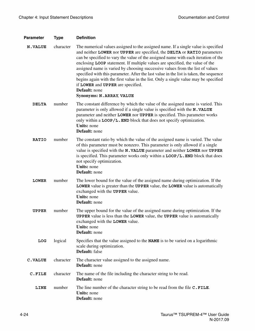
Chapter 4: Input Statement Descriptions Documentation and Control

N.VALUE character The numerical values assigned to the assigned name. If a single value is specified and neither LOWER nor UPPER are specified, the DELTA or RATIO parameters can be specified to vary the value of the assigned name with each iteration of the enclosing LOOP statement. If multiple values are specified, the value of the assigned name is varied by choosing successive values from the list of values specified with this parameter. After the last value in the list is taken, the sequence begins again with the first value in the list. Only a single value may be specified if LOWER and UPPER are specified.Default: noneSynonyms: N.ARRAY, VALUE

DELTA number The constant difference by which the value of the assigned name is varied. This parameter is only allowed if a single value is specified with the N.VALUE parameter and neither LOWER nor UPPER is specified. This parameter works only within a LOOP/L.END block that does not specify optimization.Units: noneDefault: none

RATIO number The constant ratio by which the value of the assigned name is varied. The value of this parameter must be nonzero. This parameter is only allowed if a single value is specified with the N.VALUE parameter and neither LOWER nor UPPER is specified. This parameter works only within a LOOP/L.END block that does not specify optimization. Units: noneDefault: none

LOWER number The lower bound for the value of the assigned name during optimization. If the LOWER value is greater than the UPPER value, the LOWER value is automatically exchanged with the UPPER value.Units: noneDefault: none

UPPER number The upper bound for the value of the assigned name during optimization. If the UPPER value is less than the LOWER value, the UPPER value is automatically exchanged with the LOWER value.Units: noneDefault: none

LOG logical Specifies that the value assigned to the NAME is to be varied on a logarithmic scale during optimization.Default: false

C.VALUE character The character value assigned to the assigned name. Default: none

C.FILE character The name of the file including the character string to be read.Default: none

LINE number The line number of the character string to be read from the file C.FILE.Units: noneDefault: none

Parameter Type Definition

4-24 Taurus™ TSUPREM-4™ User GuideN-2017.09

Documentation and Control Chapter 4: Input Statement Descriptions

C1 character The first in a list of character values assigned to the assigned name. The value of the assigned name is varied by choosing successive values from the list of values specified with the parameters C1 through C10. If the looping step exceeds the maximum parameter, the assigned character value is circulated from C1 again. This parameter works only within a LOOP/L.END block that does not specify optimization. Default: none

C2 character The second in a list of character values assigned to the assigned name. The value of the assigned name is varied by choosing successive values from the list of values specified with the parameters C1 through C10. This parameter works only within a LOOP/L.END block that does not specify optimization.Default: none

C3 character The third in a list of character values assigned to the assigned name. The value of the assigned name is varied by choosing successive values from the list of values specified with the parameters C1 through C10. This parameter works only within a LOOP/L.END block that does not specify optimization.Default: none

C4 character The fourth in a list of character values assigned to the assigned name. The value of the assigned name is varied by choosing successive values from the list of values specified with the parameters C1 through C10. This parameter works only within a LOOP/L.END block that does not specify optimization.Default: none

C5 character The fifth in a list of character values assigned to the assigned name. The value of the assigned name is varied by choosing successive values from the list of values specified with the parameters C1 through C10. This parameter works only within a LOOP/L.END block that does not specify optimization.Default: none

C6 character The sixth in a list of character values assigned to the assigned name. The value of the assigned name is varied by choosing successive values from the list of values specified with the parameters C1 through C10. This parameter works only within a LOOP/L.END block that does not specify optimization.Default: none

C7 character The seventh in a list of character values assigned to the assigned name. The value of the assigned name is varied by choosing successive values from the list of values specified with the parameters C1 through C10. This parameter works only within a LOOP/L.END block that does not specify optimization.Default: none

C8 character The eighth in a list of character values assigned to the assigned name. The value of the assigned name is varied by choosing successive values from the list of values specified with the parameters C1 through C10. This parameter works only within a LOOP/L.END block that does not specify optimization.Default: none

Parameter Type Definition

Taurus™ TSUPREM-4™ User Guide 4-25N-2017.09

Chapter 4: Input Statement Descriptions Documentation and Control

Description The ASSIGN statement associates a value with a name. The value is substituted for the name whenever the name appears in the input file preceded by the “@” character. The name must start with a letter and may contain only letters and numbers.

C9 character The ninth in a list of character values assigned to the assigned name. The value of the assigned name is varied by choosing successive values from the list of values specified with the parameters C1 through C10. This parameter works only within a LOOP/L.END block that does not specify optimization.Default: none

C10 character The tenth in a list of character values assigned to the assigned name. The value of the assigned name is varied by choosing successive values from the list of values specified with the parameters C1 through C10. This parameter works only within a LOOP/L.END block that does not specify optimization.Default: none

ARRAY character The prefix name for an array to store the sequential data from the external data file. The index of an array starts with 1. Default: none

IN.FILE character The identifier for the file containing the data to be stored to the ARRAY parameter. The file format must be either a TIF or a columnwise format.Default: none

DATA character The name of the data in a TIF file or the column number of the data in a columnwise file to be stored to the ARRAY parameter.Default: none

TIF logical Specifies that the IN.FILE is a TIF file.Default: false

ROW logical Specifies that the IN.FILE is a rowwise file.Default: false

COLUMN logical Specifies that the IN.FILE is a columnwise file.Default: true

IN.NVALU character The string composed of numbers, for example, “1.2 3 4.5 6.”Default: none

IN.CVALU character The string composed of character strings, for example, “a bc def g.”Default: none

C.COUNT character The name of the variable to which the number of the stored data is assigned.Default: none

Parameter Type Definition

4-26 Taurus™ TSUPREM-4™ User GuideN-2017.09

Documentation and Control Chapter 4: Input Statement Descriptions

The ASSIGN statement performs a function similar to that of the DEFINE statement, but in a way that is more convenient for many applications. Some of its advantages are:

• An ASSIGNed name can take on a different value for each iteration of a LOOP statement. Different names can be varied in unrelated ways during a single loop.

• The syntax for using ASSIGNed names is simpler than for DEFINEd names, leaving less chance for confusion or error.

• The ASSIGN statement works in the same way in TSUPREM-4 as it does in Medici and Davinci.

Varying DuringStatement

Looping

The ASSIGNed variable may be varied during statement looping by one of the following:

• A constant increment, by specifying the DELTA parameters:

LOOP STEPS=3ASSIGN NAME=X N.VAL=10 DELTA=10 PRINT

L.END

The variable X takes the values 10, 20, and 30.

• A constant ratio, by specifying the RATIO parameter:

LOOP STEPS=3ASSIGN NAME=X N.VAL=10 RATIO=10 PRINT

L.END

The variable X takes the values 10, 100, and 1000.

• A list of values from which successive values are taken during each pass through a statement loop:

LOOP STEPS=3ASSIGN NAME=X N.VAL="20, 10, 90" PRINT

L.END

The variable X takes the values 20, 10, and 90.

ASSIGN WithMathematicalExpressions

The assigned value may be specified with another variable and/or a mathematical expression as well as a constant. For example,

ASSIGN NAME=X N.VAL=0.2ASSIGN NAME=Y N.VAL=ERFC(@X) PRINTLOOP STEPS=2 ASSIGN NAME=Z N.VAL="@X+@Y, LOG10(@X*@Y)"L.END

Taurus™ TSUPREM-4™ User Guide 4-27N-2017.09

Chapter 4: Input Statement Descriptions Documentation and Control

Note:The N.VALUE (N.ARRAY) is handled as a character string; the separator of an N.VALUE is a blank or a comma character. Thus, if there is a blank character in the specified formula to N.VALUE, for example, N.VALUE=( @X + @Y ) may not be accepted. Instead, use the N.EXPRES. Since the N.EXPRES is not a character string but a number, the blank character can be accepted as long as the formula is wrapped by parentheses. If the formula is not wrapped by parentheses, even N.EXPRES disallows a blank character.

ASSIGN andOptimization

• The ASSIGNed variable specifies a parameter to be optimized when both LOWER and UPPER parameters are specified. The initial value, with which the optimization starts, is specified with the N.VALUE parameter. The optimization loop determines an appropriate value for each assigned name for each pass through the loop after the first. The range of allowed values for the assigned name is specified with the LOWER and UPPER parameters.

• The sensitivity shown after optimization is based on the value of normalized parameters to eliminate the unit dependency. The normalization is performed as follows:

Thus, the reported sensitivity value depends on the values of LOWER and UPPER.

Expansion ofASSIGNed

Variable

The combination of assigned variables is expanded from left to right. For example:

ASSIGN NAME=A C.V=TASSIGN NAME=B C.V=MASSIGN NAME=C C.V=AASSIGN NAME=D C.V=@A@B@C PRINT

The variable D is assigned with the character string TMA.

ASSIGN NAME=EF C.V=BESTASSIGN NAME=GH C.V=F$ 1)ASSIGN NAME=IJ C.V=@E@GH PRINT

ASSIGN NAME=E C.V=GOL$ 2)ASSIGN NAME=F C.V=@E@GH PRINT

At 1), E is an unknown variable and, therefore, is not expanded. @GH is expanded to the character, F. Then, @EF is expanded to the string BEST. However, at 2), E is not an unknown variable any longer so that @E is expanded to the string GOL.

Param,normParam-LOWERUPPER-LOWER-------------------------------------=

4-28 Taurus™ TSUPREM-4™ User GuideN-2017.09

Documentation and Control Chapter 4: Input Statement Descriptions

Finally, the variable F is assigned with the string GOLF, to which GOL@GH has been expanded.

Reading theExternal Data

File

The data in a TIF file or a rowwise or a columnwise file can be read through the ASSIGN statement. The data is sequentially read into the variable ARRAY to be appended with the index of which the starting number is 1. The parameter DATA specifies which data is to be read, the name of the data for a TIF file, the row number of data for a rowwise file, or the column number of data for a columnwise file. The variable defined by C.COUNT stores the number of data to be read.

ASSIGN ARRAY=VG IN.FILE=VGID.IVL TIF DATA=V(GATE)+C.COUNT=NDATA

ASSIGN ARRAY=ID IN.FILE=VGID.IVL TIF DATA=I(DRAIN)LOOP STEPS=@NDATA

ASSIGN NAME=i N.V=1 DELTA=1EXTRACT PREFIX="@VG@i @ID@i"

L.END

If the number of data is 12, the value of NDATA is 12, and each variable of VGn and IDn, in which n has the number from 1 to 12, stores the V(GATE) and I(DRAIN), respectively. The example shows how to read the .ivl (TIF format) file written by Taurus™ Medici. It prints out the data, V(GATE) versus I(DRAIN), in a vgid.ivl file.

Note:If there is already a variable with the same name as the ARRAY, the previous value of the variable is overridden. In the above example, if the variable, for example, VG1, already exists before reading the data file, the current value of VG1 is lost and replaced with the data read.

Also the character string can be read from an external file.

ASSIGN NAME=str C.FILE=text.dat LINE=10

The variable str stores the string of 10-th line in the file text.dat.

Reading theArray From a

String

The array can be read from a data string composed of either numbers or characters.

ASSIGN ARRAY=vg IN.NVALU=”0.05 1.0” C.COUNT=nvgsASSIGN ARRAY=type IN.CVALU=”linear saturat”

The numbers of the variables vg1 and vg2 are 0.05 and 1.0, respectively. The strings of the variables type1 and type2 are “linear’ and “saturat,” respectively. The variable nvgs stores the number 2 of the count of the array.

Taurus™ TSUPREM-4™ User Guide 4-29N-2017.09

Chapter 4: Input Statement Descriptions Documentation and Control

INTERMEDIATE

The INTERMEDIATE statement specifies the intermediate quantities associated with equations. Aliases for the INTERMEDIATE statement are MODEL (see Chapter 7, INTERMEDIATE, p. 7-7) or ARRAY.

INTERMEDIATE

{ SCOPE=<c>| ENDSCOPE| { NAME=<c> [EXPRESS=<c>] [SIZE=<c> [MININDEX=<c>][DEFAULT=<c>]]

[{ PRINT | DELETE }] [{ FIXNOW | UNFIXNOW }]}

Parameter Type Definition

SCOPE character The name of the scope which defines the start of the block that must end by the parameter ENDSCOPE. All intermediates within the block belong to the SCOPE.Default: none

ENDSCOPE logical Specifies to close the block defined by the SCOPE.Default: false

NAME character The intermediate name.Default: none

EXPRESS character The expression for the intermediate named by the NAME parameter. The EXPRESS parameter can specify a single expression or multiple expressions separated by commas (,). Multiple expressions are allowed only when the SIZE parameter is specified.Default: noneSynonym: VALUE

SIZE character The array size. The SIZE specification implies that the intermediate is an array, the size of which is specified by the SIZE parameter.Default: noneSynonym: LENGTH

MININDEX character The array minimum index numberDefault: 0

DEFAULT character The default initial expression for array elements. Only one expression is allowed. The DEFAULT parameter may not be specified together with the EXPRESS parameter.Default: none

PRINT logical Specifies that the values of intermediates are to be printed.Default: false

DELETE logical Specifies that the intermediate is to be removed.Default: false

4-30 Taurus™ TSUPREM-4™ User GuideN-2017.09

Documentation and Control Chapter 4: Input Statement Descriptions

Advantages ofINTERMEDIATES

The advantages of using intermediates quantities are:

• Simplifying long and complicated equations

• Avoiding the duplicated calculation of quantities used in several equations

Once the intermediates are evaluated, the calculated values are shared by all associated equations until the intermediates need to be reset

• Avoiding duplicated calculation of quantities depending only on temperature

If the intermediates depend only on temperature, they are evaluated only when the temperature changes.

• Using intermediates in the same manner as the built-in solution values in the SELECT statement.

Note:Intermediates are stored as symbolic expressions that are evaluated later (for example, when solving the model equations).

Scope Definition The parameters SCOPE and ENDSCOPE specifies the scope range within which the intermediates are applied. The scopes can be hierarchically nested.

INTERMED NAME=A1 EXPR=10INTERMED SCOPE=family INTERMED NAME=A1 EXPR=20 INTERMED SCOPE=genus1 INTERMED NAME=A1 EXPR=30 INTERMED NAME=A1 PRINT ;$(1) INTERMED ENDSCOPE INTERMED NAME=A1 PRINT ;$(2) INTERMED SCOPE=genus2 INTERMED NAME=A1 EXPR=35 INTERMED ENDSCOPEINTERMED ENDSCOPE

The (1) command prints 30 while the (2) prints 20.

The intermediates in the higher or same level scopes can be accessed from the lower level by specifying the intermediate name followed by the full path of scopes. ‘#’ is the character to separate the intermediate name and its scope path. The path string following ‘#’ always starts with ‘.’ which denote the top level.

FIXNOW logical Specifies to fix the current values of the intermediates.Default: false

UNFIXNOW logical Specifies to unfix the fixed intermediate.Default: false

Parameter Type Definition

Taurus™ TSUPREM-4™ User Guide 4-31N-2017.09

Chapter 4: Input Statement Descriptions Documentation and Control

Then the scope names from the top level to the level in which the intermediate is defined are concatenated by the character ‘.’.

In the above example,

INTERMED NAME=A1 EXPR=10INTERMED SCOPE=family INTERMED NAME=A1 EXPR=20 INTERMED SCOPE=genus1 INTERMED NAME=A1 EXPR=30 INTERMED NAME=A1 INTERMED NAME=A1#. PRINT ;$(1) INTERMED NAME=A1#.family PRINT ;$(2) INTERMED ENDSCOPE INTERMED NAME=A1 PRINT INTERMED SCOPE=genus2 INTERMED NAME=A1 EXPR=35 INTERMED NAME=A1#.family.genus1 PRINT ;$(3) INTERMED ENDSCOPEINTERMED ENDSCOPEINTERMED PRINT ;$(4)

(1) prints A1 value in the top level, that is, 10. (2) prints 20 in the scope ‘family’, one level lower than the top. (3) prints 30 which is defined in the scope ‘genus1’, the neighbor scope ‘genus2’. (4) prints all intermediates. The full path of each intermediate is written in ‘Scope’ column. If the full path name is longer than 10 characters, it is truncated as shown in ‘A1#.family.genus1’ and ‘A1#.family.genus2’.

---------- ---------- --------- ------------------------------------- ----------Intermed Scope Type Expression Value

---------- ---------- --------- ------------------------------------- ----------A1 . CONSTANT 10 10A1 .family CONSTANT 20 20A1 .family.ge CONSTANT 30 30A1 .family.ge CONSTANT 35 35---------- ---------- --------- ------------------------------------- ----------

The following example shows the case using the array type (see the details for the array type in Array Values, p. 4-34):

INTERMED NAME=R1 SIZE=2 EXPR=”10,20”INTERMED SCOPE=lev1 INTERMED NAME=R1 SIZE=3 EXPR=”30,40,R1#.[1]” INTERMED SCOPE=lev2a INTERMED NAME=R1 SIZE=2 EXPR=”R1#.[0], R1#.lev1[0]” INTERMED ENDSCOPE INTERMED SCOPE=lev2b INTERMED NAME=R1 SIZE=2 + EXPR=”R1#.lev1.lev2a[1], 50” INTERMED ENDSCOPEINTERMED ENDSCOPEINTERMED PRINT ;$ (1)

4-32 Taurus™ TSUPREM-4™ User GuideN-2017.09

Documentation and Control Chapter 4: Input Statement Descriptions

The array intermediates in higher or neighbor scopes can be accessed by appending the full path to the array name. (1) prints as follows:

Array Name : R1, Scope: .---------- --------- ------------------------------------------------ ----------

Index Type Expression Value---------- --------- ------------------------------------------------ ----------[0] CONSTANT 10 10[1] CONSTANT 20 20---------- --------- ------------------------------------------------ ----------

Array Name : R1, Scope: .lev1---------- --------- ------------------------------------------------ ----------

Index Type Expression Value---------- --------- ------------------------------------------------ ----------[0] CONSTANT 30 30[1] CONSTANT 40 40[2] CONSTANT R1#.[1] 20---------- --------- ------------------------------------------------ ----------

Array Name : R1, Scope: .lev1.lev2a---------- --------- ------------------------------------------------ ----------

Index Type Expression Value---------- --------- ------------------------------------------------ ----------[0] CONSTANT R1#.[0] 10[1] CONSTANT R1#.lev1[0] 30---------- --------- ------------------------------------------------ ----------

Array Name : R1, Scope: .lev1.lev2b---------- --------- ------------------------------------------------ ----------

Index Type Expression Value---------- --------- ------------------------------------------------ ----------[0] CONSTANT R1#.lev1.lev2a[1] 30[1] CONSTANT 50 50---------- --------- ------------------------------------------------ ----------

Value Type When the expression is described by the EXPRESS parameter, the value type is automatically determined to be one of the following:

• CONSTANT The value is a constant number. It is recalculated whenever any other constant intermediate is redefined.

INTERMED NAME=C1 EXPRESS=1.0 ;$1INTERMED NAME=C2 EXPRESS=C1 ;$2INTERMED NAME=C1 EXPRESS=2.0 ;$3

In the third line, the C2 value is changed from 1.0 to 2.0.

• PARAMETER The value depends only on temperature. The value will be recalculated whenever the temperature changes.

INTERMED NAME=P1 EXPRESS=1E-5*exp(-2.0/kt) ;$1INTERMED NAME=P2 EXPRESS=P1 ;$2

The values of the P1 and P2 intermediates are always the same. The value type of the intermediate P2 is PARAMETER.

• SOLUTION The value is a node solution or an edge solution. The node solution type specifies that the quantity varies on nodes. The edge solution type represents the quantity evaluated on the edges between nodes.

INTERMED NAME=S1 EXPRESS=BORON+PHOS ;$1INTERMED NAME=S2 EXPRESS=MIN(S1,1E21);$2

The value type of the intermediate S2 is SOLUTION.

Taurus™ TSUPREM-4™ User Guide 4-33N-2017.09

Chapter 4: Input Statement Descriptions Documentation and Control

If the type of an intermediate is changed by reassignment, the value types of the others associated with the intermediate are also reviewed and changed, if needed.

INTERMED NAME=P1 EXPRESS=1E-5*exp(-2.0/kt) ;$1INTERMED NAME=P2 EXPRESS=P1 ;$2INTERMED NAME=P1 EXPRESS=2.0 ;$3

In the third line, the P2 value type is changed to CONSTANT.

Array Values The SIZE parameter specifies that the intermediate is an array as well as its array size. The values for the array elements are provided by the string. In the string, each element is separated by a comma (,) in the EXPRESS parameter. When the DEFAULT parameter is specified instead of the EXPRESS parameter, all elements are initialized to the DEFAULT parameter. The DEFAULT parameter allows only a single expression. The expression type can be CONSTANT, PARAMETER, and also SOLUTION. If the number of data items listed in the EXPRESS parameter is smaller than the SIZE parameter, the undefined array elements are assigned with N/A values. Conversely, if the number of data items listed are greater than the SIZE parameter, all the data items in the list beyond the SIZEth item are ignored. You can also define the starting value of array indices with the MININDEX parameter. The default value of the MININDEX parameter is 0. Each array element can have a different value type.

INTERMED NAME=a SIZE=3 MININDEX=-1 +EXPRESS=”1,BORON+PHOS,exp(-1.0/KT)” PRINT

The array size 3 and the minimum index -1 means that the first array element is a[-1] and the last one is a[1]. The array elements are assigned with the different value types CONSTANT, SOLUTION, and PARAMETER. The output shows:

Multidimensional arrays are defined in a similar way to single arrays. The array dimension is determined by the number of sizes listed in the SIZE parameter. Each number listed corresponds to the size of each dimension. Similarly, the minimum numbers of each index are specified with the string specified by the MININDEX parameter.

INTERMED NAME=b SIZE=”2,3” MININDEX=”0,-1” + EXPRESS=”1,2,3,SUM(i,1,10,i^2),KT,BORON” PRINT

There are two sizes listed in the SIZE parameter, 2 and 3. That means it is a 2D array. The size of the first dimension is 2 and its index starts from 0. The size of the second dimension is 3, and its minimum index is -1. Thus, the first array element is b[0][-1] and the last one is b[1][1].

Array Name : a, Scope: .---------- --------- -------------------------------- ----------

Index Type Expression Value---------- --------- -------------------------------- ----------[-1] CONSTANT 1 1[0] SOLUTION BORON+PHOS[1] PARAMETER exp(-1.0/KT) 2.01e-05---------- --------- -------------------------------- ----------

4-34 Taurus™ TSUPREM-4™ User GuideN-2017.09

Documentation and Control Chapter 4: Input Statement Descriptions

The output shows:

Getting Array Values Use the bracket symbol ([]) to get the value of an array element.

INTERMED NAME=a SIZE=2 EXPRESS=”10,20” ;$1INTERMED NAME=b EXPRESS=a[1] ;$2INTERMED NAME=c SIZE=3 EXPRESS=”a[0],b,30” ;$3INTERMED NAME=c PRINT

The array element can be the other array element as well as an intermediate, as shown in the third line. The above example prints out as:

Redefinition of ArrayElements

Redefine array elements in the same manner as non-array intermediates.

INTERMED NAME=a SIZE=”3,2” +EXPRESS=”1,2,temp,4,arsenic,0”

INTERMED NAME=a[0][1] EXPRESS=boron

The a[0][1] is changed to the solution variable boron from the constant 2.

Effect Due toRedefinition

Changing the value type of an array element affects the types of the other intermediates.

INTERMED NAME=a SIZE=”3,2” +EXPR=”1,2,temp,4,arsenic,0” ;$1

INTERMED NAME=b EXPR=sum(i,0,0,sum(j,0,1,a[i][j])) ;$2INTERMED NAME=c EXPR=sum(i,0,1,sum(j,0,1,a[i][j])) ;$3INTERMED NAME=d EXPR=sum(i,1,2,sum(j,0,1,a[i][j])) ;$4INTERMED PRINT ;$5INTERMED NAME=a[0][1] EXPR=boron ;$6INTERMED PRINT ;$7

Array Name : b, Scope: .---------- --------- -------------------------------- ----------

Index Type Expression Value---------- --------- -------------------------------- ----------[0][-1] CONSTANT 1 1[0][0] CONSTANT 2 2[0][1] CONSTANT 3 3[1][-1] CONSTANT SUM(i,1,10,i^2) 385[1][0] PARAMETER KT 0.0925[1][1] SOLUTION BORON---------- --------- -------------------------------- ----------

Array Name : c, Scope: .---------- --------- -------------------------------- ----------

Index Type Expression Value---------- --------- -------------------------------- ----------[0] CONSTANT a[0] 10[1] CONSTANT b 20[2] CONSTANT 30 30---------- --------- -------------------------------- -----------

Taurus™ TSUPREM-4™ User Guide 4-35N-2017.09

Chapter 4: Input Statement Descriptions Documentation and Control

In the fifth line, the output shows:

At line six, the value of the array element a[0][1] is changed to a solution variable, boron from a constant of 1. It implies that the value type of a[0][1] is changed to SOLUTION from CONSTANT. Thus, it affects the value types of the intermediates b and c of which the expressions include a[0][1]. In the seventh line, it prints out:

Comparison toASSIGN

The ASSIGN statement assigns numeric or string values. The values assigned by the ASSIGN statement are never changed unless they are re-specified by ASSIGN. The value assigned by the ASSIGN statement is substituted for the name preceded by the ‘@’ character. The differences between the INTERMED and ASSIGN statements are as follows:

---------- ---------- --------- ------------------------------------- ----------Intermed Scope Type Expression Value---------- ---------- --------- ------------------------------------- ----------b . CONSTANT sum(i,0,0,sum(j,0,1,a[i][j])) 3c . PARAMETER sum(i,0,1,sum(j,0,1,a[i][j])) 1.08e+03d . SOLUTION sum(i,1,2,sum(j,0,1,a[i][j]))---------- ---------- --------- ------------------------------------- ----------

---------- ---------- --------- ------------------------------------- ----------Intermed Scope Type Expression Value---------- ---------- --------- ------------------------------------- ----------b . SOLUTION sum(i,0,0,sum(j,0,1,a[i][j]))c . SOLUTION sum(i,0,1,sum(j,0,1,a[i][j]))d . SOLUTION sum(i,1,2,sum(j,0,1,a[i][j]))---------- ---------- --------- ------------------------------------- ----------

Differences INTERMED ASSIGN

Numeric value type INTERMED NAME=a EXPRESS=exp(2) ASSIGN NAME=a N.VALUE=exp(2)

String value type Not available ASSIGN NAME=a C.VALUE=”TS4”

Solution value type INTERMED NAME=a EXPRESS=boron Not available

Array definition INTERMED NAME=b +EXPRESS=”4,5” SIZE=2

ASSIGN ARRAY=b +IN.NVALU=”4,5”

Array dimension Multidimension allowed one dimension only

Default minimum index of arrays

0 1

Getting values ab[1]

@a@b1

Evaluation of expres-sions

Expression are saved and evaluated only when necessaryINTERMED NAME=a EXPRESS=1INTERMED NAME=b EXPRESS=aINTERMED NAME=a EXPRESS=2INTERMED NAME=b PRINT ;$ b=2

SELECT TEMP=800INTERMED NAME=c EXPRESS=tempSELECT TEMP=900INTERMED NAME=c PRINT;$ c=1173

Expressions are evaluated immediatelyASSIGN NAME=a N.VALUE=1ASSIGN NAME=b N.VALUE=@aASSIGN NAME=a N.VALUE=2ASSIGN NAME=b PRINT ;$ b=1

SELECT TEMP=800ASSIGN NAME=c N.VALUE=tempSELECT TEMP=900ASSIGN NAME=c PRINT;$ c=1073

4-36 Taurus™ TSUPREM-4™ User GuideN-2017.09

Documentation and Control Chapter 4: Input Statement Descriptions

Snapshot The INTERMED expression is evaluated by call-by-reference. For example,

INTERMED NAME=A1 EXPR=10INTERMED NAME=A2 EXPR=A1 PRINT ;$(1)INTERMED NAME=A1 EXPR=20INTERMED NAME=A2 PRINT ;$(2)

At (1), A2 stores the memory address of A1 instead of the value of A1, 10. Thus (2) shows that A2 value is 20 because the value of A1 is changed to 20.

The parameter FIXNOW snapshots and fixes the current values. On the other hand, the parameter UNFIXNOW unfixes the fixed INTERMED. For example,

INTERMED NAME=A1 EXPR=10

$ The following statement is same as:$ INTERMED NAME=A2 EXPR=A1$ INTERMED NAME=A2 FIXNOWINTERMED NAME=A2 EXPR=A1 FIXNOW

INTERMED NAME=A1 EXPR=20INTERMED NAME=A2 PRINT ;$(1)INTERMED NAME=A2 UNFIXNOW PRINT ;$(2)

The command (1) and (2) print 10 and 20 respectively. As shown in the following output of the commands (1) and (2), the name of a fixed intermediate is followed by the character ‘*’;

INTERMED NAME=A2 PRINT

---------- ---------- --------- ------------------------------------- ----------Intermed Scope Type Expression Value

---------- ---------- --------- ------------------------------------- ----------A2* . CONSTANT A1 10---------- ---------- --------- ------------------------------------- ----------

INTERMED NAME=A2 UNFIXNOW PRINT

---------- ---------- --------- ------------------------------------- ----------Intermed Scope Type Expression Value

---------- ---------- --------- ------------------------------------- ----------A2 . CONSTANT A1 20---------- ---------- --------- ------------------------------------- ----------

The following example shows how to compare as-implant and post-anneal profiles. The field name DIMPLANT stores the as-implant dopant concentration. The BIMPLANT and PIMPLANT intermediates store the boron and phosphorus as-implant profiles respectively.

INTERMED NAME=BIMPLANT EXPR=DIMPLANTINTERMED NAME=PIMPLANT EXPR=DIMPLANT

IMPLANT BORON DOSE=1E15 ENERGY=10$ Snapshot boron as-implant profileINTERMED NAME=BIMPLANT FIXNOW

IMPLANT PHOSPHOR DOSE=2E14 ENERGY=30$ Snapshot phosphorus as-implant profileINTERMED NAME=PIMPLANT FIXNOWDIFFUSE TEMP=900 TIME=10

$ PLOT COMPARISON BEFORE/AFTER DIFFUSIONSELECT Z=LOG10(BIMPLANT)PLOT.1D X.V=0 TOP=22 BOT=15 RIGHT=0.5 COLOR=2

Taurus™ TSUPREM-4™ User Guide 4-37N-2017.09

Chapter 4: Input Statement Descriptions Documentation and Control

SELECT Z=LOG10(BORON)PLOT.1D X.V=0 !CL !AX COLOR=2 LINE=2SELECT Z=LOG10(PIMPLANT)PLOT.1D X.V=0 !CL !AX COLOR=4 LINE=2SELECT Z=LOG10(PHOSPHOR)PLOT.1D X.V=0 !CL !AX COLOR=4 LINE=2

Load/SaveIntermediates

Using INTERMED is the convenient method to manipulate solution data. By saving the expressions and calculated values of intermediates to TIF or TS4 structure format files, you can use the intermediates continuously after loading them. You also can plot the intermediate values in visualizer tools such as Taurus Visual.

The intermediates are saved when the parameter INTERMED is turned on in the SAVEFILE command.

SAVEFILE OUT.FILE=test.tif TIF INTERMED ;$ TIF formatSAVEFILE OUT.FILE=test.sav INTERMED ;$ TS4 format

The intermediates are not loaded when the parameter INTERMED is turned off in the INITIALIZE or LOADFILE commands.

INITIALIZE IN.FILE=test.tif TIF ^INTERMEDINITIALIZE IN.FILE=test.sav ^INTERMEDLOADFILE IN.FILE=test.tif TIF ^INTERMEDLOADFILE IN.FILE=test.sav ^INTERMED

Example To save the equilibrium concentration and supersaturation of interstitial:

INTERMED NAME=ISTAR EXPR=CI.STARINTERMED NAME=IRATIO EXPR=CI.RATIOMETHOD PD.FULLMESH DY.SURF=0.001 LY.SURF=0.001 DY.ACT=0.05 LY.ACT=0.5INITDEPOSIT OXIDE THICKNES=0.001IMPLANT BORON DOSE=1E15 ENERGY=10DIFFUSE TEMP=700 TIME=0.1/60 SAVEFILE OUT.FILE=test.tif TIF INTERMED

4-38 Taurus™ TSUPREM-4™ User GuideN-2017.09

Documentation and Control Chapter 4: Input Statement Descriptions

ECHO

The ECHO statement prints its parameters, evaluating arithmetic expressions.

Description The ECHO statement prints the given <string> on the standard output. Defined abbreviations are substituted into the string. If the result is a valid arithmetic expression, it is evaluated. (See COMMENT, p. 4-7 and SELECT, p. 4-151.) Otherwise, the resulting string value is printed.

Examples • The statements:

DEFINE W 2.0ECHO The width is W - 0.5ECHO W - 0.5

print the two lines:

The width is 2.0 - 0.51.5

to your terminal and to the standard output file. The first ECHO statement prints a string because its argument is not a valid arithmetic expression. The second ECHO statement shows evaluation of a valid expression.

• The statement:

ECHO ( 15.0 - 12.0 * exp( 4.0 - 2.0 / 6.0 ) )

prints:

-454.455

which is the value of the arithmetic expression.

ECHO <string>

Taurus™ TSUPREM-4™ User Guide 4-39N-2017.09

Chapter 4: Input Statement Descriptions Documentation and Control

OPTION

The OPTION statement sets terminal and plotting options.

OPTION [DEVICE=<c>] [PLOT.OUT=<c>] [ {QUIET | NORMAL | VERBOSE | DEBUG} ] [INFORMAT] [DIAGNOST] [STRICT] [ECHO] [EXECUTE] [V.COMPAT]

[ZIP.FILE] [ZIP.EXE=<c>] [UNZIP.EX=<c>] [ZIP.SUFF=<c>][AUTOSAVE=<n>]

Parameter Type Definition

DEVICE character The name of the graphics device to be used for plotting. Default: none

PLOT.OUT character The file to which graphics output is sent. If the name is preceded by a “+”, the output is appended to an existing file; otherwise, an existing file is overwritten or a new file is created.Default: noneSynonyms: FILE.SAV, PLOT.SAV

QUIET logical Print a minimum of information in the standard output and the output listing file. Default: the current value; initially false

NORMAL logical Print the “normal” amount of information in the standard output and the output listing file. Default: the current value; initially true

VERBOSE logical Print more than the normal amount of information in the standard output and the output listing file. Default: the current value; initially false

DEBUG logical Include all available debugging information in the standard output and the output listing file. Default: the current value; initially false

INFORMAT logical Send additional output to the informational output file. Default: the current value; initially false

DIAGNOST logical Send additional output to the diagnostic output file. Default: the current value; initially false

STRICT logical Verify the syntax strictlyDefault: the current value; initially false

ECHO logical Echo each input statement to the standard output as it is processed. Default: the current value; initially true

4-40 Taurus™ TSUPREM-4™ User GuideN-2017.09

Documentation and Control Chapter 4: Input Statement Descriptions

Selecting aGraphics Device

Use the DEVICE parameter to specify the type of graphics device to be used for plotting. The device types known to the program are described in the s4pcap file; a listing of the available devices is given in Appendix B. If no DEVICE is specified, a default device is chosen as follows:

1. If the environment variable DEFPDEV is defined as the name of a valid plot device, its value is used as the plot device.

2. Otherwise, if the environment variable TERM is defined as the name of a valid plot device, its value is used as the plot device.

3. Otherwise, the DEFAULT device in the s4pcap file is used. Note that the s4pcap file can be modified to make the DEFAULT device refer to any available real plotting device (see Appendix B).

RedirectingGraphics Output

Graphics output normally goes to your terminal or to the file specified in the s4pcap file. In either case, the output can be redirected to the file specified by the PLOT.OUT parameter. This allows graphics output to be saved for later processing or display. When graphics output is redirected by PLOT.OUT, it does not appear on your terminal or in the file specified in s4pcap.

Printed Output The QUIET, NORMAL, VERBOSE, and DEBUG parameters control the amount of printed output generated by the program. NORMAL mode is assumed when the program begins. Output from the VERBOSE and DEBUG modes is not needed during typical usage of TSUPREM-4 and may be difficult to interpret.

EXECUTE logical Execute each input statement as it is read. If EXECUTE is false, input statements are checked for syntax but not executed. Default: the current value; initially true

V.COMPAT number Change certain models and algorithms to be compatible with the specified version of TSUPREM-4.Default: the current version of TSUPREM-4

ZIP.FILE logical Specifies that all files to be saved and loaded are in a compressed format.Default: false

ZIP.EXE character String to command to compress.Default: “gzip -c”

ZIP.FILE logical Specify that all files to be saved and loaded are in a compressed format.Default: false

AUTOSAVE number Specify the level of automatic save when a simulation stops abnormally by a syntax error or an internal fatal error or CTRL-C.Units: noneDefault: 0

Parameter Type Definition

Taurus™ TSUPREM-4™ User Guide 4-41N-2017.09

Chapter 4: Input Statement Descriptions Documentation and Control

Informationaland Diagnostic

Output

The INFORMAT and DIAGNOST parameters specify whether informational and diagnostic output are written to the appropriate files. If output to one of these files is disabled before any information is written, the file is not created. The default initialization file s4init sets both these parameters false, disabling both files.

Echoing andExecution of

Input Statements

The ECHO parameter controls whether input statements are listed on the standard output (usually your terminal) as they are processed. By default, this option is turned on. The EXECUTE parameter controls whether statements are executed as they are encountered. If EXECUTE is false, statements are checked for syntax but not processed. This is useful for doing a preliminary syntax check of an input file. The DEFINE, UNDEFINE, FOREACH, SOURCE, RETURN, OPTION, and STOP statements are always executed, regardless of the setting of the EXECUTE option.

VersionCompatibility

The V.COMPAT parameter is used to improve compatibility with older versions of TSUPREM-4. When an older version number is specified, certain models and algorithms from the older version are used in place of the current models and algorithms. Only some changes between versions are reversed by using V.COMPAT.

Strict SyntaxCheck

Stricter syntax verification of the input keywords has been implemented. Strict syntax verification can be switched on in the input file by the command OPTION STRICT. By turing on STRICT, a vocabulary keyword can not be a substring of the input keyword. This is valid for up to 8 letters of the input keywords; all other letters are not verified. For example, TSUPREM-4 recognizes MOMEN in the input file as MOMENT keyword, but does not recognize MOMENTS. The strict syntax check detects the mistake that users made when they confused a built-in keyword and an input string. For example, users define a new impurity BSIGE by:

IMPURITY IMP=BSIGE NEW IMPL.TAB=TR.BORON C.INIT=1E5

Since the new impurity BSIGE is different from the built-in impurity B, the implantation of BSIGE must be given by:

IMPLANT IMP=BSIGE DOSE=1E15 ENERGY=30

Note that BSIGE is given as an input string for the IMP built-in keyword. However, when BSIGE is given like a built-in keyword, TSUPREM-4 recognizes B for BSIGE because the ‘SIGE’ of BSIGE is ignored. For example,

IMPLANT BSIGE DOSE=1E15 ENERGY=30

the above statement performs not BSIGE implant, but B implant. Turning on STRICT catches this kind of mistake.

Automatic Save When a simulation stops abnormally by a syntax error or an internal fatal error or CTRL-C, the AUTOSAVE mode stores the simulation result before such an accident so that users can continue the simulation after fixing the error without rerunning whole simulation again. The AUTOSAVE mode is specified in the OPTION statement.

4-42 Taurus™ TSUPREM-4™ User GuideN-2017.09

Documentation and Control Chapter 4: Input Statement Descriptions

Three modes are provided as follows:

• OPTION AUTOSAVE=0

No autosave mode.

• OPTION AUTOSAVE=1

Recommended. Save the latest result among CPU intensive processes such as DIFFUSE, EPITAXY or IMPLANT before abnormal stop.

• OPTION AUTOSAVE=2

Save the latest result among DIFFUSE, EPITAXY, IMPLANT, STRUCTURE, ETCH, DEPOSIT, DEVELOP, EXPOSE, PROFILE or STRESS before abnor-mal stop

The file format to save temporary solutions is the TSUPREM-4 structure file format and the file is named with

_<prefix of input file name>_

For example, if the input file name is test.inp, the saved file is

_test_

Note: AUTOSAVE does not work for the unexpected exceptions, such as segmentation faults or bus errors caused by memory conflicts.

Load/Save Filesin Compressed

Format

The size of a saved file tends to increase as the simulation models used for the recent process technology becomes complicated. In addition, saving intermediates increases the file size. Saving the text files such as TIF or TS4 structure files in compressed format reduces the size by the factor of 7~8, which depends on the compression program.

The parameter ZIP.EXE and UNZIP.EX defines the command for compression and uncompression, respectively. The ZIP.SUFF defines the suffix of a compressed file name.

The parameter ZIP.FILE specifies to save/load the files in compressed format:

OPTION ZIP.FILE

The compression/uncompression also can be given by turning on/off the ZIP.FILE parameter on each statement of the INITIALIZE, LOADFILE, SAVEFILE, and PROFILE commands.

Examples • The following statement causes the graphics output to be produced for a Tektronix 4100-series terminal and appended to the file plotsave:

OPTION DEVICE=4100 PLOT.OUT="+plotsave"

• Additional information is printed on the standard output with the statement:

OPTION VERBOSE

Taurus™ TSUPREM-4™ User Guide 4-43N-2017.09

Chapter 4: Input Statement Descriptions Documentation and Control

• Enhanced compatibility with TSUPREM-4 Version 6.4 can be obtained with:

OPTION V.COMPAT=6.4

• In s4init, gzip command is set for compression as follows:

OPTION ZIP.EXE=”gzip -c” UNZIP.EX=”gunzip -c” + ZIP.SUFF=gz

For using the UNIX compress command:

OPTION ZIP.EXE=”compress -c” +UNZIP.EX=”uncompress -c” ZIP.SUFF=Z

• When ZIP.FILE is turned on in the OPTION statement, the file is saved in the compressed format even when ZIP.FILE is not specified in SAVEFILE:

OPTION ZIP.FILEINITIAL BORON=1E15SAVEFILE OUT.FILE=test.sav ;$--> test.sav.gz

• If you do not want to compress the specific file, then turn off ZIP.FILE on the specific command:

OPTION ZIP.FILEINITIAL BORON=1E15SAVEFIL OUT.FILE=test1.sav ;$--> test1.sav.gzIMPLANT ARSENIC DOSE=1E14 ENERGY=30 SAVEFIL OUT.FILE=test2.tif TIF ;$--> test2.tif.gzDIFFUSE TEMP=900 TIME=10SAVEFIL OUT.FILE=test3.tif TIF ^ZIP.FILE

;$--> test3.tif

• When loading the file, the file is assumed to be compressed if the parameter ZIP.FILE was turned on in the OPTION statement.

OPTION ZIP.FILEINITIAL IN.FILE=test1.tif TIF ;$<-- test1.tif.gzINITIAL IN.FILE=test2.tif TIF ^ZIP.FILE

;$<-- test2.tif

OPTION ^ZIP.FILE INITIAL IN.FILE=test1.tif TIF ;$<-- test1.tifINITIAL IN.FILE=test2.tif TIF ZIP.FILE

;$<-- test2.tif.gz

4-44 Taurus™ TSUPREM-4™ User GuideN-2017.09

Documentation and Control Chapter 4: Input Statement Descriptions

DEFINE

The DEFINE statement defines strings for substitution in subsequent input statements.

DEFINE [<name> <body>]

Description This statement defines the name <name> as an abbreviation for the string <body>. Any time <name> appears in an input line as a separate token (see below), <body> is substituted. This allows long, often-used sequences to be abbreviated. DEFINE without any parameters lists the current definitions. To undefine a <name>, use the UNDEFINE statement.

Format andSyntax

The DEFINE statement uses the following format and syntax. The defined <name> can only contain letters and digits. A name is recognized and expanded only if it is preceded and followed by one of the following separators: space, tab, newline, <, >, &, “;”, !, {, }, =, “,”, $, @, or (. To ensure that defined names are recognized in arithmetic expressions, the name should be preceded and followed by spaces, and the entire expression enclosed in parentheses. Expansion of abbreviations can be forced by preceding the defined name with the “@” character; in this case the name can also be enclosed in braces to separate it from surrounding characters. Older versions of the program used the “$” character to force expansion; this usage is now obsolete, although it is still recognized by the program. Within a character string, you can force recognition of a defined name by enclosing the name in braces (“{” and “}”) and preceding the left brace with the “@” (or “$”) character.

Substitution of abbreviations is inhibited by the “%” character. When “%” is encountered in an input line, expansion of abbreviations is inhibited for the rest of the line, except when forced by the “@” (or “$”) character.

Examples • The following statements define and use the name LIMITS:

DEFINE LIMITS X.MIN=0.0 X.MAX=5.0 Y.MIN=0.0 Y.MAX=20.0PLOT.2D LIMITS

The parameter specifications for X.MIN, X.MAX, Y.MIN, and Y.MAX are substituted whenever the name LIMITS is encountered. Thus, the PLOT.2D statement is equivalent to

PLOT.2D X.MIN=0.0 X.MAX=5.0 Y.MIN=0.0 Y.MAX=20.0

• For the statements:

DEFINE W 2.0ECHO 1-WECHO 1-@W

the output is:

1-W -1

Taurus™ TSUPREM-4™ User Guide 4-45N-2017.09

Chapter 4: Input Statement Descriptions Documentation and Control

In the first ECHO statement, “-” is not recognized as a separator. In the second ECHO statement, the “@” forces expansion of the abbreviation W.

• The statements:

DEFINE PROC C41SAVEFILE OUT.FILE=MOS@{PROC}A.DAT

save the structure in file MOSC41A.DAT. The defined name PROC is inserted in the middle of a text string with the “@{}” construct to force expansion.

Usage Notes • Abbreviations are expanded whenever they are encountered, including in DEFINE and UNDEFINE statements. The expanded version of an abbreviation is not checked for further abbreviations, however. For example,:

DEFINE a bDEFINE c a

defines both a and c as “b,” but:

DEFINE a b%DEFINE c a

defines a as “b” and c as “a.” References to c produce “a,” which is not expanded to “b.”

• Similarly, to redefine an name, you must use the “%” character. For example:

DEFINE a bDEFINE a c

defines a as “b” and b as “c.” To define a as “c,” use:

DEFINE a b%DEFINE a c

The substitution of “b” for a in the second line is prevented by the “%” character.

• When undefining an abbreviation, be sure to use the “%” character on the UNDEFINE statement:

DEFINE a bUNDEFINE a

does not work, because the UNDEFINE statement is expanded to

UNDEFINE b

and b is not defined. To undefine a, use:

%UNDEFINE a

• A line beginning with “$” is not treated as a COMMENT statement if the “$” is immediately followed by the name of a defined abbreviation. The expansion of the abbreviation is substituted. Thus, in the statements

DEFINE THIS 1.0$THIS IS NOT A COMMENT

4-46 Taurus™ TSUPREM-4™ User GuideN-2017.09

Documentation and Control Chapter 4: Input Statement Descriptions

the value 1.0 is substituted for the name THIS in the second statement, giving:

1.0 IS NOT A COMMENT

which results in a syntax error.

• It is not possible to assign a null value to a name with the DEFINE statement.

• Use care when choosing names to be defined. You normally want to avoid using names that are also valid statement or parameter names. For example, given:

DEFINE TIME 20DIFFUSE TIME=TIME

The second statement is expanded as:

DIFFUSE 20=20

resulting in a syntax error.

• For many applications, it is easier to use the ASSIGN and LOOP statements instead of DEFINE and FOREACH. See ASSIGN, p. 4-23 and LOOP/L.END, p. 4-16.

Taurus™ TSUPREM-4™ User Guide 4-47N-2017.09

Chapter 4: Input Statement Descriptions Documentation and Control

UNDEFINE

The UNDEFINE statement undefines a previously defined abbreviation.

Description The UNDEFINE statement is used to turn off previously defined abbreviations. The character string <name> gives the name of the abbreviation to be deleted. The statement should normally be given as %UNDEFINE; the “%” is required to prevent substitution for abbreviations in the UNDEFINE statement itself.

The UNDEFINE statement is also useful for correcting mistakes made with the DEFINE statement. For more examples of the UNDEFINE statement, see DEFINE, p. 4-45.

Example The statements:

DEFINE W 2.0ECHO 1 - W%UNDEFINE WECHO 1 - W

produce the output:

-11 - W

RedefinedParameter

Names

The UNDEFINE statement is most often needed when a parameter name has been redefined. For example, you may wish to do the following:

DEFINE COMPRESS VISCOUSSOURCE OXIDE1%UNDEFINE COMPRESSSOURCE OXIDE2

This forces any METHOD COMPRESS statements in file OXIDE1 to be interpreted as METHOD VISCOUS statements. By undefining the name COMPRESS, this substitution is not made when executing file OXIDE2.

UNDEFINE <name>

4-48 Taurus™ TSUPREM-4™ User GuideN-2017.09

Documentation and Control Chapter 4: Input Statement Descriptions

CPULOG

The CPULOG statement controls the logging of CPU usage.

Description The CPULOG statement instructs the program to record the amount of CPU time used in various internal operations. The information appears on the standard output and in the output listing file unless it is redirected with the OUT.FILE parameter. Most CPU-intensive operations report the time used.

Examples • The following statement enables reporting of CPU statistics to the standard output and the output listing file:

CPULOG LOG

• The following statement enables CPU statistics reporting, and stores the output in the file timefile.

CPU LOG OUT.FILE=timefile

Limitations The accuracy of the times depends on the computer being used.

A resolution of 1/60 s is typical. Some systems cannot report CPU time at all. Reported times are zero for those systems. Timing for a complete TSUPREM-4 simulation is best obtained using operating system commands, such as the TIME command in the UNIX C-shell.

CPULOG

[LOG] [OUT.FILE=<c>]

Parameter Type Definition

LOG logical Enables logging of CPU usage when true; disables CPU logging when false.Default: true

OUT.FILE character The file to which the CPU log is written.Default: standard outputSynonym: CPUFILE

Taurus™ TSUPREM-4™ User Guide 4-49N-2017.09

Chapter 4: Input Statement Descriptions Documentation and Control

HELP

The HELP statement prints a summary of statement names and parameters.

Description The HELP statement prints a summary of statement names and parameters to the standard output. If no <name> is given, a summary of statement names is printed. If the name of a statement is given, a summary of parameters for that statement is printed. The parameter summary includes the name type, and default for each parameter.

Example The statement:

HELP DIFFUSION

prints a summary of the parameters on the DIFFUSION statement.

Notes • The default values printed by the HELP statement are not always helpful. This is especially true for statements that specify the values of model coefficients. These statements usually ignore parameters that are not specified rather than use the default values. The default value is likewise meaningless for parameters that must be specified on a statement.

• Help is not always available for statements that use nonstandard syntax (that is, special statements).

!(Exclamation Mark)

The exclamation mark allows to call a UNIX shell command. For example:

SAVEFILE OUT.FILE=a.tif TIF$ copy a.tif to b.tif by calling unix command ‘cp’!cp a.tif b.tif

HELP

[<name>]

4-50 Taurus™ TSUPREM-4™ User GuideN-2017.09

Device Structure Specification Chapter 4: Input Statement Descriptions

Device Structure SpecificationThe following statements specify the device structure used by TSUPREM-4:

Statement Name Description Page

MESH Sets grid spacing scale factor and defaults for automatic grid generation.

p. 4-52

LINE Specifies a grid line in a rectangular mesh. p. 4-56

ELIMINATE Specifies grid lines to be removed from parts of the mesh.

p. 4-58

BOUNDARY Sets boundary conditions for a rectangular mesh.

p. 4-61

REGION Sets material types for a rectangular mesh. p. 4-63

INITIALIZE Initializes a rectangular mesh or reads mesh and solution information from a file.

p. 4-68

LOADFILE Reads mesh and solution information from a file.

p. 4-74

SAVEFILE Writes mesh and solution information to a file. p. 4-77

STRUCTURE Reflects, truncates, extends, or unrefines a structure.

p. 4-82

MASK Reads mask information from a file. p. 4-87

PROFILE Reads a 1D doping profile from a file. p. 4-89

ELECTRODE Specifies the name and position of electrodes. p. 4-98

Taurus™ TSUPREM-4™ User Guide 4-51N-2017.09

Chapter 4: Input Statement Descriptions Device Structure Specification

MESH

The MESH statement specifies a grid spacing scale factor and default values for controlling automatic grid generation.

MESH

[GRID.FAC=<n>] [DX.MAX=<n>] [DX.MIN=<n>] [DX.RATIO=<n>] [LY.SURF=<n>] [DY.SURF=<n>] [LY.ACTIV=<n>] [DY.ACTIV=<n>] [LY.BOT=<n>] [DY.BOT=<n>] [DY.RATIO=<n>] [FAST]

Parameter Type Definition

GRID.FAC number A factor by which all grid spacing specifications are multiplied. The scaling occurs when the spacings are used (not when they are specified.)Units: noneDefault: the current value

DX.MAX number The maximum grid spacing in the x direction (that is, between vertical grid lines) in the default horizontal grid. This is the spacing to be used far from mask edges. This spacing is multiplied by GRID.FAC when it is used.Units: micronsDefault: the current value

DX.MIN number The minimum grid spacing in the x direction (that is, between vertical grid lines) in the default horizontal grid. This is the spacing to be used at mask edges. This spacing is multiplied by GRID.FAC when it is used.Units: micronsDefault: the current value

DX.RATIO number The ratio by which grid spaces are increased from DX.MIN to DX.MAX in the default horizontal grid.Units: micronsDefault: the current value

LY.SURF number The depth of the surface region in the default vertical grid.Units: micronsDefault: the current value

DY.SURF number The grid spacing in the y direction (that is, between horizontal grid lines) in the surface region of the default vertical grid. This spacing is used between y=0 and y=LY.SURF. This spacing is multiplied by GRID.FAC when it is used.Units: micronsDefault: the current value

LY.ACTIV number The depth of the bottom of the active region in the default vertical grid.Units: micronsDefault: the current value

4-52 Taurus™ TSUPREM-4™ User GuideN-2017.09

Device Structure Specification Chapter 4: Input Statement Descriptions

Description The MESH statement controls the automatic generation of simulation grids for TSUPREM-4. A grid is generated whenever an INITIALIZE statement without an IN.FILE parameter is processed. Automatic grid generation is used unless an appropriate set of LINE statements has been processed since the previous INITIALIZE statement was processed. Grids can be automatically generated in both the x and y directions, and automatic grid generation in one direction can be combined with manual grid specification on the other direction.

Grid CreationMethods

A simulation grid for TSUPREM-4 can be created in one of four ways:

• It can be read from a saved structure file, using the INITIALIZE or LOADFILE statements.

• It can be generated from user-specified LINE, REGION, BOUNDARY, and ELIMINATE statements.

• It can be generated automatically from parameters supplied on the MESH statement and from information read from mask data files.

• The last two methods can be combined, using one of the methods for generating the horizontal grid and the other method for generating the vertical grid.

DY.ACTIV number The grid spacing in the y direction (that is, between horizontal grid lines) at the bottom of the active region in the default vertical grid. The grid spacing varies geometrically between DY.SURF at LY.SURF and DY.ACTIV at LY.ACTIV. This spacing is multiplied by GRID.FAC when it is used.Units: micronsDefault: the current value

LY.BOT number The depth of the bottom of the structure in the default vertical grid.Units: micronsDefault: the current value

DY.BOT number The grid spacing in the y direction (that is, between horizontal grid lines) at the bottom of the structure in the default vertical grid. This spacing is multiplied by GRID.FAC when it is used.Units: micronsDefault: the current value

DY.RATIO number The ratio by which grid spaces are increased from DY.ACTIV to DY.BOT in the default vertical grid.Units: micronsDefault: the current value

FAST logical Specifies that 1D simulation is used until an etch step creates a structure that varies in the x direction. The structure is automatically converted to 2D status when required.Default: true

Parameter Type Definition

Taurus™ TSUPREM-4™ User Guide 4-53N-2017.09

Chapter 4: Input Statement Descriptions Device Structure Specification

If no LINE statements are supplied before an INITIALIZE statement, a grid is generated automatically. If LINE X statements are supplied, they are used (instead of automatic generation) for the horizontal grid; if LINE Y statements are supplied, they are used to generate the vertical grid.

Horizontal GridGeneration

The automatic generation of the horizontal grid depends on whether mask information has been read with the MASK statement.

• If no mask information has been read, the default horizontal grid consists of two (vertical) grid lines located at y=0.0 and y=1.0. This produces a quasi 1D simulation.

• If mask information is available, it is used with the DX.MIN, DX.MAX, and DX.RATIO parameters to automatically generate a horizontal grid.

The horizontal grid has a spacing between (vertical) grid lines of approximately DX.MIN at mask edges, expanding to a spacing of DX.MAX at distances far from any mask edge. The DX.RATIO parameter specifies the rate at which the spacing increases away from mask edges. The minimum and maximum grid locations are set to the minimum and maximum x coordinates for which mask information is supplied in the mask data file(s).

For a complete description of the grid generation process, see Chapter 3, Automatic Grid Generation, p. 3-5.

Vertical GridGeneration

The automatically generated vertical grid is controlled by the various LY and DY parameters.

• LY.SURF, LY.ACTIV, and LY.BOT specify the locations of the bottom of the surface region, active region, and structure, respectively.

• DY.SURF, DY.ACTIV, and DY.BOT specify the grid spacings at these locations.

Between the top of the structure and LY.SURF, the grid spacing DY.SURF is used. The spacing increases geometrically (that is, with a constant ratio) from DY.SURF at LY.SURF to DY.ACTIV at LY.ACTIV. The spacing expands to DY.BOT below LY.ACTIV. The DY.RATIO parameter specifies the rate at which the spacing increases below DY.ACTIV.

In a automatically generated vertical grid, vertical grid lines deeper than LY.ACTIV are eliminated, to increase the speed of the simulation. It is assumed that only point defects diffuse below this depth and that the point defect profiles are approximately constant in the horizontal direction, so that the low horizontal resolution does not cause significant loss of accuracy in the simulation.

For a complete description of the grid generation process see Chapter 3, Automatic Grid Generation in the Y-Direction, p. 3-7.

4-54 Taurus™ TSUPREM-4™ User GuideN-2017.09

Device Structure Specification Chapter 4: Input Statement Descriptions

Scaling the GridSpacing

The GRID.FAC parameter multiplies all grid spacing specifications, including those on the MESH, LINE, DEPOSITION, and EPITAXY statements. The default values of all grid spacings are set so that GRID.FAC=1.0 produces a moderately fine grid, useful for reasonably, accurate simulations. For faster simulations, GRID.FAC should be given a value greater than 1.0. For more accurate simulations, GRID.FAC should be reduced as needed.

The GRID.FAC parameter modifies the values of other parameters in the following ways:

• The DX.MIN, DX.MAX, DY.SURF, DY.ACTIV, and DY.BOT parameters on the MESH statement are multiplied by GRID.FAC.

• The DY and ARC.SPAC parameters on the DEPOSITION and EPITAXY statements are multiplied by GRID.FAC.

• The SPACES parameter on the DEPOSITION and EPITAXY statements is divided by GRID.FAC.

• The DY.OXIDE on the METHOD statement and the DY.DEFAU parameter on the MATERIAL statement are multiplied by GRID.FAC (the modification takes place when the parameters are used, not when they are specified).

Note:Moderation should be used in adjusting GRID.FAC—reducing the value from 1.0 to 0.1 increases the grid density by a factor of 10 in each direction, increasing the node count by a factor of 100 and the simulation time by a factor of more than 100.

1D Mode Normally, when a mesh is generated or read from a file, it is examined to determine whether there is any variation of the structure or solution values in the x direction. If there is no variation, then simulation proceeds in 1D mode. By setting the FAST parameter false, the use of 1D mode is disabled. If 1D mode is already in use, the structure is converted to 2D.

Examples • The following MESH statements could be used in the s4init file to set the default parameters for automatic grid generation:

MESH DX.MIN=0.1 DX.MAX=0.4 DX.RATIO=1.5MESH LY.SURF=0.1 DY.SURF=0.03 LY.ACTIV=4.0 +

DY.ACTIV=0.3 LY.BOT=200 DY.BOT=100 DY.RATIO=1.5

• The following statement cuts all grid spacings to one half their specified value, giving twice the specified grid density in the horizontal and vertical directions:

MESH GRID.FAC=0.5

Taurus™ TSUPREM-4™ User Guide 4-55N-2017.09

Chapter 4: Input Statement Descriptions Device Structure Specification

LINE

The LINE statement specifies a horizontal or vertical mesh line in a non-uniform rectangular grid.

Description This statement specifies the position and spacing of one line in a rectangular mesh. A complete mesh specification consists of a group of LINE statements followed by ELIMINATE statements (optional), REGION and BOUNDARY statements (optional), and an INITIALIZE statement.

TSUPREM-4 uses an inverted Cartesian coordinate system, with x increasing from left to right and y increasing from the top surface of the structure into the substrate.

Placing GridLines

Grid lines are placed at the locations specified on LINE statements. Additional lines are added automatically so that the final grid spacing varies geometrically between the SPACING values at the user-specified lines. The spacing ratio between adjacent pairs of grid lines is guided by the value of the RATIO parameter on the INITIALIZE statement.

The final grid spacing may be slightly larger than that specified on the LINE statement because of the need for an integral number of spaces; it may be much smaller than specified to satisfy constraints imposed by neighboring grid lines and the RATIO parameter. A complete description of the grid setup process is given in Chapter 3, Explicit Specification of Grid Structure, p. 3-3.

LINE {X | Y} LOCATION=<n> [SPACING=<n>] [TAG=<c>]

Parameter Type Definition

X logical If true, then LOCATION specifies the x coordinate of a vertical grid line.Default: false

Y logical If true, then LOCATION specifies the y coordinate of a horizontal grid line.Default: false

LOCATION number The y coordinate of a horizontal grid line or the x coordinate of a vertical grid line. Units: micronsDefault: none

SPACING number The local grid spacing. Units: micronsDefault: none

TAG character A name used to refer to this grid line on a BOUNDARY or REGION statement. Default: none

4-56 Taurus™ TSUPREM-4™ User GuideN-2017.09

Device Structure Specification Chapter 4: Input Statement Descriptions

Example The following statements include three user-specified vertical grid lines and two user-specified horizontal grid lines:

LINE X LOCATION=0 SPACING=1LINE X LOCATION=1 SPACING=0.1LINE X LOCATION=2 SPACING=1LINE Y LOCATION=0 SPACING=0.02LINE Y LOCATION=3 SPACING=0.5

After processing with RATIO=1.5, TSUPREM-4 produces a mesh with vertical grid lines at 0.0, 0.42, 0.69, 0.88, 1.0, 1.12, 1.31, 1.58, and 2.0. Around the center, the spacing is 0.12, approximately what was requested. At each edge, the spacing is 0.42, because that is as coarse as it could get without exceeding the allowed ratio between adjacent grid spaces. If the allowed ratio were 9, then you would get one space of 0.9 microns and one space of 0.1 micron on each side of the center line.

Additional Notes Below are some additional notes on the LINE statement.

Structure Depth andPoint Defect Models

When the PD.TRANS or PD.FULL or NSTREAM=5 point defect model is to be used, the structure should be deep to accommodate the deep diffusion of point defects. A depth of 50 to 200 microns is suggested. ELIMINATE statements can be used to eliminate all but two vertical grid lines deep in the structure. When ELIMINATE statements are used with a coarse vertical grid spacing, the computational overhead of using a deep structure can be made negligible.

• Maximum Number of Nodes and Grid Lines

The program can handle up to 100,000 nodes; this includes one node per grid point, plus one node for each exposed point and another node for each point on a boundary between two materials. Thus, the grid must be smaller than 100,000 points. In addition, the initial grid must not have more than 1000 grid lines in either the x or y direction.

Default Regions andBoundaries

No tags are required if the default regions and boundary conditions are to be used, that is, if the initial structure consists entirely of silicon with only the top surface exposed.

Taurus™ TSUPREM-4™ User Guide 4-57N-2017.09

Chapter 4: Input Statement Descriptions Device Structure Specification

ELIMINATE

The ELIMINATE statement eliminates mesh nodes along lines in a grid structure over a specified rectangular region.

Description The ELIMINATE statement is used to eliminate nodes in regions of the device structure where the grid would otherwise be more dense than necessary. The ROWS parameter specifies that every second row of nodes within the specified region is to be removed. Similarly, the COLUMNS parameter specifies that every second column of nodes within the specified region is to be removed.

ELIMINATE

{ROWS | COLUMNS} [X.MIN=<n>] [X.MAX=<n>] [Y.MIN=<n>] [Y.MAX=<n>]

Parameter Type Definition

ROWS logical Specifies that horizontal lines of nodes are eliminated. Default: false Synonym: X.DIREC

COLUMNS logical Specifies that vertical lines of nodes are eliminated. Default: false Synonym: Y.DIREC

X.MIN number The minimum horizontal location of the rectangular region over which nodes are eliminated. Units: microns Default: the minimum horizontal location of the device structureSynonym: X.LOW

X.MAX number The maximum horizontal location of the rectangular region over which nodes are eliminated. Units: microns Default: the maximum horizontal location of the device structure Synonym: X.HIGH

Y.MIN number The minimum vertical location of the rectangular region over which nodes are eliminated. Units: microns Default: the minimum vertical location of the device structureSynonym: Y.LOW

Y.MAX number The maximum vertical location of the rectangular region over which nodes are eliminated. Units: microns Default: the maximum vertical location of the device structureSynonym: Y.HIGH

4-58 Taurus™ TSUPREM-4™ User GuideN-2017.09

Device Structure Specification Chapter 4: Input Statement Descriptions

The ELIMINATE statement can only be used after the LINE statements and before the INITIALIZE statement.

Note:Elimination of grid lines takes place during initial structure generation. The ELIMINATE statement cannot be used to eliminate grid lines after the INITIALIZE statement has been processed.

It is frequently a good idea to plot and examine the initial grid after the LINE X, LINE Y, ELIMINATE, and INITIALIZE statements to verify the desired grid structure before proceeding.

Reducing GridNodes

The ELIMINATE statement can be very useful for reducing the number of grid nodes (and hence execution time), especially for large structures. In particular, you might use LINE X and LINE Y statements to define a large structure that would exceed the limit of 100,000 nodes, then eliminate enough rows and columns to bring the final number of nodes under 100,000.

OverlappingRegions

If you get an error message stating that one of the ELIMINATE statements is causing a mesh generation error, it is due to overlapping or adjacent eliminate regions. For best results when performing multiple eliminations over a structure, either:

1. Do the multiple eliminations over identical regions of the structure, or

2. Avoid overlapping or adjacent eliminate regions (that is, separate the regions by at least one grid line).

If you must have overlapping eliminate regions, best results are obtained if the ELIMINATE statements define successively smaller regions. That is, start with the largest region, then eliminate additional nodes in subsets of that region. If you need to eliminate over partially overlapping regions, best results are obtained if you minimize the amount of overlap.

Examples • The following statement eliminates every other row of nodes over the entire structure:

ELIMINATE ROWS

The same result could be obtained by changing the locations and grid spacings on the LINE Y statements.

• The following statement eliminates every other column of nodes over the full width of the structure, but only for values of y greater than 4.5 microns:

ELIMINATE COLUMNS Y.MIN=4.5

Taurus™ TSUPREM-4™ User Guide 4-59N-2017.09

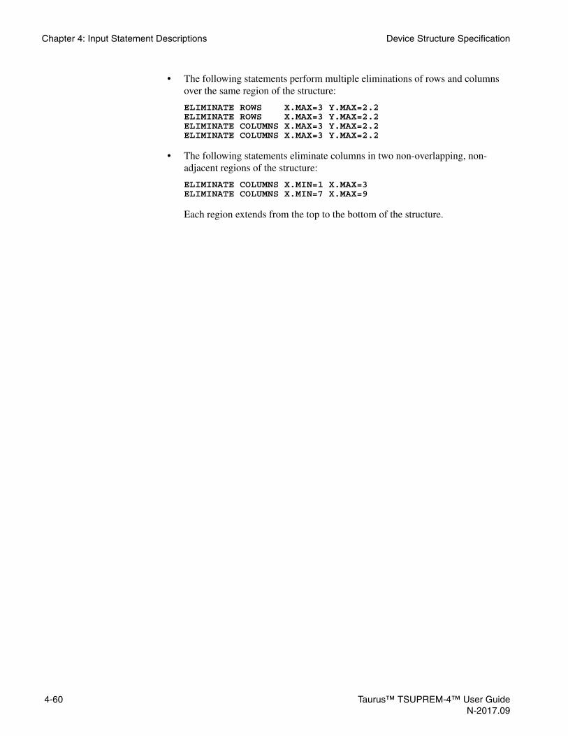
Chapter 4: Input Statement Descriptions Device Structure Specification

• The following statements perform multiple eliminations of rows and columns over the same region of the structure:

ELIMINATE ROWS X.MAX=3 Y.MAX=2.2ELIMINATE ROWS X.MAX=3 Y.MAX=2.2ELIMINATE COLUMNS X.MAX=3 Y.MAX=2.2ELIMINATE COLUMNS X.MAX=3 Y.MAX=2.2

• The following statements eliminate columns in two non-overlapping, non-adjacent regions of the structure:

ELIMINATE COLUMNS X.MIN=1 X.MAX=3ELIMINATE COLUMNS X.MIN=7 X.MAX=9

Each region extends from the top to the bottom of the structure.

4-60 Taurus™ TSUPREM-4™ User GuideN-2017.09

Device Structure Specification Chapter 4: Input Statement Descriptions

BOUNDARY

The BOUNDARY statement specifies a boundary condition along an edge of the structure.

Description This statement specifies the boundary conditions that apply at the surfaces in a rectangular mesh. Two surface types are recognized: exposed and reflecting.

Exposed surfaces normally correspond to the top of the wafer. Deposition, oxidation, and out-diffusion occur at exposed surfaces. Impurity predeposition also happens at exposed surfaces, as do defect recombination and generation. The default boundary condition for the sides and the back of the structure is reflecting, while the default for the top surface is exposed. Thus the BOUNDARY statement is not required for most simulations. The tags specified with the XLO, XHI, YLO, and YHI parameters correspond to tags specified on the LINE statements used to define the mesh. XLO, XHI, YLO, and YHI must specify one entire edge of the structure. It is not permissible to specify part of an edge, a region of nonzero area, or a line in the interior of the structure.

Limitations At present, the BOUNDARY statement is only useful in special situations, due to the following limitations in the various processing steps:

• DEPOSITION only works on the top and right side (when exposed) of the structure, and may fail if the bottom of the structure is exposed.

BOUNDARY {REFLECTI | EXPOSED} XLO=<c> XHI=<c> YLO=<c> YHI=<c>

Parameter Type Definition

REFLECTI logical The specified boundary is reflecting. Default: false

EXPOSED logical The specified boundary is exposed. Default: false

XLO character The tag corresponding to the left edge of the boundary. Default: none

XHI character The tag corresponding to the right edge of the boundary. Default: none

YLO character The tag corresponding to the top edge of the boundary. Default: none

YHI character The tag corresponding to the bottom edge of the boundary. Default: none

Taurus™ TSUPREM-4™ User Guide 4-61N-2017.09

Chapter 4: Input Statement Descriptions Device Structure Specification

• ETCH with the TRAPEZOI and OLD.DRY options assumes that the exposed surface is etched from the top. Etching with the TRAPEZOI and OLD.DRY options may fail if the sides or bottom of the structure are exposed.

• Ion implantation always occurs on the top surface.

• DIFFUSION works correctly on all exposed surfaces, but the analytical and VERTICAL oxidation models assume that oxidation only occurs at the top surface.

The BOUNDARY statement is only used in setting up the initial structure. It cannot be used to change a boundary condition after the structure has been initialized.

Example The following statement specifies that the top of the mesh is the exposed surface:

BOUNDARY EXPOSED XLO=left XHI=right YLO=surf YHI=surf

The tags left, right, and surf must have been previously specified on the LINE statements used to define the mesh. See the description of the LINE statement on p. 4-56.

4-62 Taurus™ TSUPREM-4™ User GuideN-2017.09

Device Structure Specification Chapter 4: Input Statement Descriptions

REGION

The REGION statement specifies the material type of a mesh region.

REGION { MATERIAL=<c> | SILICON | OXIDE | OXYNITRI | NITRIDE | POLYSILI |

PHOTORES | ALUMINUM } { (XLO=<c> XHI=<c> YLO=<c> YHI=<c>) |

(NEW.MATE=<c> [KEEP] { ( X=<n> Y=<n> ) |

( IMPURITY=<c> [MIN.CONC=<n>] [MAX.CONC=<n>] )}

)}

Parameter Type Definition

MATERIAL character The specified region is defined to be of the named material.Default: none

SILICON logical The specified region is defined to be silicon. Default: false

OXIDE logical The specified region is defined to be oxide. Default: false

OXYNITRI logical The specified region is defined to be oxynitride. Default: false

NITRIDE logical The specified region is defined to be nitride. Default: false

POLYSILI logical The specified region is defined to be polysilicon. Default: false

PHOTORES logical The specified region is defined to be photoresist. Default: false

ALUMINUM logical The specified region is defined to be aluminum. Default: false

XLO character The tag specifying the left edge of the region to be defined. Default: none

XHI character The tag specifying the right edge of the region to be defined. Default: none

YLO character The tag specifying the top edge of the region to be defined. Default: none

YHI character The tag specifying the bottom edge of the region to be defined. Default: none

Taurus™ TSUPREM-4™ User Guide 4-63N-2017.09

Chapter 4: Input Statement Descriptions Device Structure Specification

Description This statement specifies the material type of rectangular subregions when generating a rectangular mesh. REGION statements appear after LINE statements but before the INITIALIZE statement. The default material is silicon; if no REGION statements are specified, the entire initial structure is assumed to be silicon.

The tags referenced on REGION statements must be defined on the preceding LINE statements.

RedefiningMaterial of the

Region

Material of the specific region can be redefined. Region names are not defined during simulation, because regions can be created, removed or merged. So a region can be specified by three parameters: material of the region and X and Y coordinates of the point inside the region. New material is specified by the NEW.MATE statement. It should be one of predefined material names or a name of material, defined by the MATERIAL command before the REGION command. Option KEEP, being specified, keeps previous solution in the region. By default, all values are reset to the default for new material.

NEW.MATE character Specifies new material in the region, which is defined by the REGION statement.Default: false

KEEP logical This option, being defined, keeps impurity and defect concentrations for previous material, when it is replaced by the new one.Default: false

X number x-coordinate of the point inside the region, the material of which should be changed.Units: micronsDefault: none

Y number y-coordinate of the point inside the region, the material of which should be changedUnits: micronsDefault: none

IMPURITY character The name of the impurity to be used for the region generation. The region in which the IMPURITY concentration is within the range between MIN.CONC and MAX.CONC values becomes the NEW.MATE region.Default: none Synonym: INTERMED

MIN.CONC number The minimum concentration of the IMPURITY field to specify the region to become a NEW.MATE region.Default:

MAX.CONC number The maximum concentration of the IMPURITY field to specify the region to become a NEW.MATE region.Default:

Parameter Type Definition

1 1038×–

1 1038×

4-64 Taurus™ TSUPREM-4™ User GuideN-2017.09

Device Structure Specification Chapter 4: Input Statement Descriptions

RegionGeneration

Based On Fields

The material type of the region defined by the range of impurity solutions can be replaced with another material type. For example, the following command creates the oxide region inside silicon region where the oxygen concentration exceeds

.

REGION MATERIAL=SILICON NEW.MAT=OXIDE +IMPURITY=OXYGEN MIN.CONC=1E18

You can use, not only a solution field, but also a user-defined intermediate field. The intermediate must be fixed before using it for the INTERMED parameter. For example:

INTERMED NAME=MyField EXPR=10*exp(-X*X/0.1)INTERMED NAME=MyField FIXNOWREGION MATERIAL=SILICON NEW.MAT=OXIDE +

INTERMED=MyField MIN.CONC=5.0

Examples The following statement defines the region bounded by the x coordinates left and right and the y coordinates surf and back to be silicon. See the description of the LINE statement on p. 4-56.

REGION SILICON XLO=left XHI=right YLO=surf YHI=back

• The following statement redefines material of a region. Previous material was oxide, new material is oxynitride. Region is defined by it’s previous material and point inside the region.

REGION OXIDE X=0.6 Y=1.2 NEW.MATE=OXYNITRIDE

Note:Use the KEEP option carefully, because some impurities and defects from the previous material may not exist in the new material.

• In SOI device, the buried oxide is grown by the thermal diffusion following high energy oxygen implantation. The simulation for such an oxidation that takes place inside bulk silicon is not an easy task, especially when the structure to be oxygen-implanted is not uniform. So you might want to create the buried oxide region within the implanted oxygen concentration that exceeds a critical value. Or more physically, you might want to insert a thin buried oxide layer and then do oxidation by solving the reaction equations between silicon and buried oxides. Figure 4-2 shows the structure before and after the buried oxide formation.

impurity new imp=oxygen at.num=8.0 at.wt=15.999 c.init=1e5 !pd.pair impl.tab=fluorine

implant imp=oxygen dose=1e15 energy=60region mat=silicon new.mat=oxide imp=oxygen

min.conc=3e19

1 1018

cm3–×

Taurus™ TSUPREM-4™ User Guide 4-65N-2017.09

Chapter 4: Input Statement Descriptions Device Structure Specification

Figure 4-2 Structure before/after the buried oxide formation

• In the oxidation simulation for cylindrical silicon structure, the circular silicon structure can be easily made with the REGION command, instead of the piecewise linear multiple etching commands for circular shape (see Figure 4-3).

MESH !FASTLINE X LOC=-1.0 SPAC=0.05 TAG=LEFTLINE X LOC=1.0 SPAC=0.05 TAG=RIGHTLINE Y LOC=-0.6 SPAC=0.05 TAG=TOPLINE Y LOC=2 SPAC=0.05 TAG=BOXLINE Y LOC=3 SPAC=0.05REGION OXIDE XLO=LEFT XHI=RIGHT YLO=TOP YHI=BOX

INITINTERMED NAME=CIRCLE FIXNOW EXPR=”SQRT(X*X+Y*Y)”REGION MATERIAL=OXIDE NEW.MAT=SILICON +

INTERMED=CIRCLE MAX=0.5INTERMED NAME=PILLAR FIXNOW +

EXPR="(X>-0.01&&X<0.01&&Y>0.49&&Y<2.1)"REGION MAT=OXIDE NEW.MAT=SILICON +

INTERMED=PILLAR MIN=0.5ETCH OXIDE ALL

4-66 Taurus™ TSUPREM-4™ User GuideN-2017.09

Device Structure Specification Chapter 4: Input Statement Descriptions

Figure 4-3 Oxidation simulation for cylindrical silicon structure

Taurus™ TSUPREM-4™ User Guide 4-67N-2017.09

Chapter 4: Input Statement Descriptions Device Structure Specification

INITIALIZE

The INITIALIZE statement sets up the initial structure for a simulation:

INITIALIZE

{ ( IN.FILE=<c> [INTERMED] [ZIP.FILE]{ ( [SCALE=<n>] [FLIP.Y] ) |

( TIF [ REGION=<c> NEW.MATE=<c> [KEEP] ] )}

) |( [WIDTH=<n> [DX=<n>]] [ {<111> | <110> | <100> | ORIENTAT=<n>} ]

[{ROT.SUB=<n> | X.ORIENT=<n>}] [RATIO=<n>] [LINE.DAT] [TEMPERAT=<n>])

}[ IMPURITY=<c> { I.CONC=<c> | I.RESIST=<n> } ][MATERIAL=<c>] [ANTIMONY=<n>] [ARSENIC=<n>] [BORON=<n>] [PHOSPHOR=<n>][{CONCENTR | RESISTIV}]

Parameter Type Definition

IN.FILE character Name of a saved structure file. If this parameter is omitted, a rectangular grid is generated, using previously specified LINE, ELIMINATE, REGION, and BOUNDARY statements. Default: noneSynonym: INFILE

INTERMED logical Load intermediatesDefault: true

ZIP.FILE logical Specifies that the loaded file is in a compressed formatDefault: false

SCALE number The mesh read in from IN.FILE is scaled by this factor. Units: noneDefault: 1.0

FLIP.Y logical Specifies that the input structure is to be reflected about y=0. Default: false

TIF logical Specifies that the input file is a TIF (Technology Interchange Format) file.Default: false

REGION character Specifies a REGION in the structure, read from the TIF file, in which material should be redefinedDefault: false

NEW.MATE character Specifies new material in the region, which is defined by the REGION statementDefault: false

4-68 Taurus™ TSUPREM-4™ User GuideN-2017.09

Device Structure Specification Chapter 4: Input Statement Descriptions

KEEP logical This option, being defined, keeps impurity and defect concentrations for previous material, when it is replaced by the new oneDefault: false

WIDTH number The width of the initial structure. (Only used if no LINE X statements are specified.)Units: micronsDefault: the width of the MASK information, if any, or 1.0

DX number The grid spacing to use in the x direction.Units: micronsDefault: the current value of DX.MAX from the MESH statement

<111> logical Specifies that the crystalline orientation of the silicon substrate is <111>.Default: false

<110> logical Specifies that the crystalline orientation of the silicon substrate is <110>.Default: false

<100> logical Specifies that the crystalline orientation of the silicon substrate is <100>.Default: True, if no other orientation is specified.

ORIENTAT number The crystalline orientation of the silicon substrate. Only 100, 110, and 111 are recognized. Units: none Default: 100 Synonym: Y.ORIENT

ROT.SUB number The rotation of the substrate about the y axis. The reference orientation (ROT.SUB=0) is defined such that the x axis points in a <110> direction. Not allowed to be less than zero and bigger than 180 degrees.Units: degreesDefault: 0.0

X.ORIENT number The crystalline orientation of the x axis. This must be a 3-digit integer value.Units: noneDefault: 110

RATIO number The maximum ratio of adjacent grid spacings to be used in generating a grid.Units: noneDefault: 1.5Synonym: INTERVAL

LINE.DAT logical Specifies that the location of each x and y grid line be listed on the standard output and in the output listing file. Default: false

TEMPERAT number The initial temperature of the structureUnits: degreesDefault: 800

Parameter Type Definition

Taurus™ TSUPREM-4™ User Guide 4-69N-2017.09

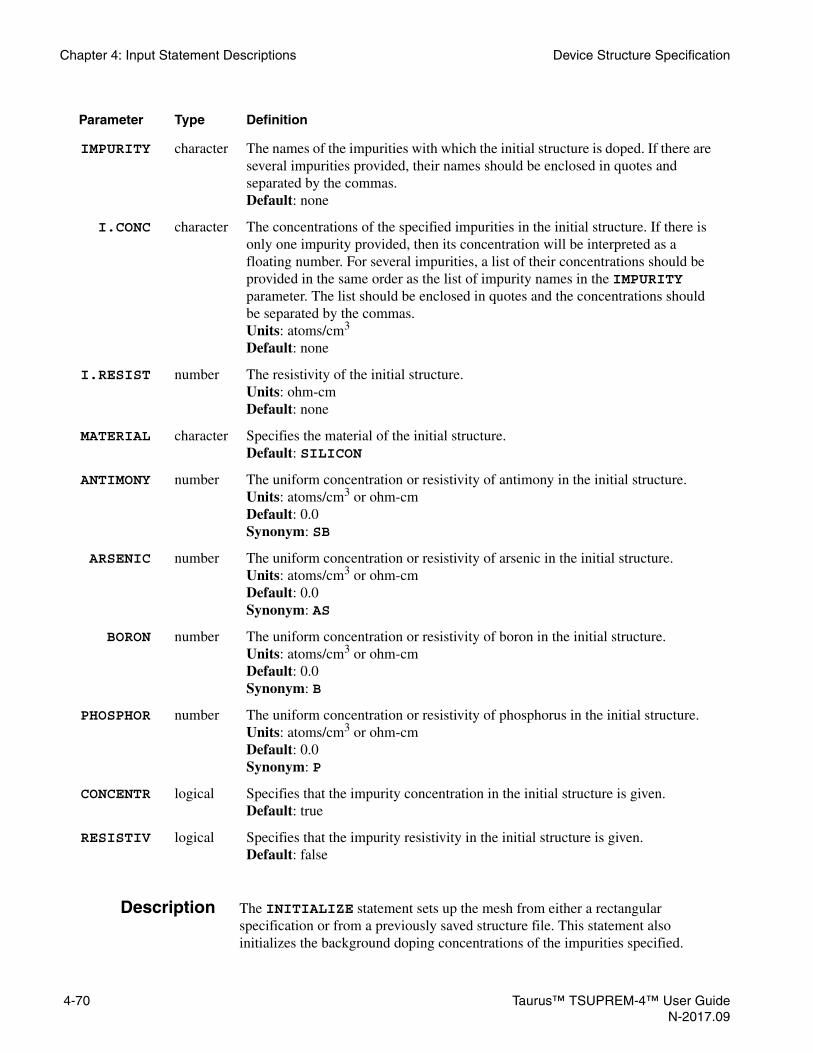
Chapter 4: Input Statement Descriptions Device Structure Specification

Description The INITIALIZE statement sets up the mesh from either a rectangular specification or from a previously saved structure file. This statement also initializes the background doping concentrations of the impurities specified.

IMPURITY character The names of the impurities with which the initial structure is doped. If there are several impurities provided, their names should be enclosed in quotes and separated by the commas.Default: none

I.CONC character The concentrations of the specified impurities in the initial structure. If there is only one impurity provided, then its concentration will be interpreted as a floating number. For several impurities, a list of their concentrations should be provided in the same order as the list of impurity names in the IMPURITY parameter. The list should be enclosed in quotes and the concentrations should be separated by the commas.Units: atoms/cm3

Default: none

I.RESIST number The resistivity of the initial structure.Units: ohm-cmDefault: none

MATERIAL character Specifies the material of the initial structure.Default: SILICON

ANTIMONY number The uniform concentration or resistivity of antimony in the initial structure. Units: atoms/cm3 or ohm-cmDefault: 0.0Synonym: SB

ARSENIC number The uniform concentration or resistivity of arsenic in the initial structure. Units: atoms/cm3 or ohm-cmDefault: 0.0Synonym: AS

BORON number The uniform concentration or resistivity of boron in the initial structure. Units: atoms/cm3 or ohm-cmDefault: 0.0Synonym: B

PHOSPHOR number The uniform concentration or resistivity of phosphorus in the initial structure. Units: atoms/cm3 or ohm-cmDefault: 0.0Synonym: P

CONCENTR logical Specifies that the impurity concentration in the initial structure is given.Default: true

RESISTIV logical Specifies that the impurity resistivity in the initial structure is given.Default: false

Parameter Type Definition

4-70 Taurus™ TSUPREM-4™ User GuideN-2017.09

Device Structure Specification Chapter 4: Input Statement Descriptions

Mesh Generation If IN.FILE is not specified, a rectangular mesh is generated. If LINE statements have been specified for the x or y direction, they are used along with any ELIMINATE, BOUNDARY, and REGION statements and the value of the RATIO parameter to generate the mesh in that direction. If no LINE statements are specified for the y direction, a default y mesh is generated. If no LINE statements are specified for the x direction, and WIDTH is specified, a mesh of the requested width is generated, with spacing given by DX. If no LINE X statements are given and WIDTH is not specified, the width is taken from mask information read with a preceding MASK statement, if any. Otherwise, a one-micron wide structure with a grid spacing of one micron (that is, one grid space wide) is generated.

See Chapter 3, Grid Structure, p. 3-3 for a complete description of the mesh generation process. The locations of the generated grid lines are listed if LINE.DAT is true.

Previously SavedStructure Files

A mesh read from a file must be in either TSUPREM-4 format or Technology Interchange Format (TIF). Meshes read from TSUPREM-4 files can be scaled or flipped about y=0 by specifying the SCALE or FLIP.Y parameters, respectively.

When a structure is read from a file, the last processing temperature as well as the choice of silicon substrate orientation, oxidation model, and point defect model are automatically set through information stored in the file. You need not respecify these parameters after reading in a structure file at the start of a simulation.

CrystallineOrientation

The crystalline orientation of any silicon regions in a generated structure can be specified by <100>, <110>, or <111> parameters. The ORIENTAT parameter is also accepted, for compatibility with older versions of the program. The specified orientation is used for all single-crystal silicon regions in the simulation, whether present in the initial structure or deposited later. By default, the x axis points in a <110> direction. This can be changed by specifying a rotation about the y axis (ROT.SUB) or the crystal orientation of the x axis (X.ORIENT).

The orientation parameters do not apply when reading a structure from a file; the orientation of the saved structure is used instead.

Specifying InitialDoping

The ANTIMONY, ARSENIC, BORON, and PHOSPHOR parameters can be used to specify the initial resistivity or impurity concentrations in the structure. Any combination of these parameters can be specified if impurity concentrations are given (CONCENTR true), but only one impurity can be specified if the resistivity is given (RESISTIV true). Impurities can also be specified by name (in the case of a single impurity) or by a list of names (in the case of multiple impurities) with the IMPURITY parameter; I.CONC or I.RESIST are used to specify the concentrations of impurities or resistivity, respectively, associated with the named impurities.

If multiple impurities are specified, their concentrations should be specified as a list of numbers with I.CONC parameter. The order of concentrations in the list

Taurus™ TSUPREM-4™ User Guide 4-71N-2017.09

Chapter 4: Input Statement Descriptions Device Structure Specification

should follow the order of the impurity names, specified with the IMPURITY parameter.

The I.RESIST parameter can be used only if a single impurity is specified by the IMPURITY parameter. The resistivity is calculated from tables of mobility as a function of doping concentration. These tables are described in Appendix A, Table A-56, p. -20.

Although the source of the grid (read or generated) and the specification of doping are independent, the doping specification is normally used when a grid is generated but not when a grid is read from a file.

RedefiningMaterial of the

Region

If structure is loaded from the TIF file, you can redefine the material of the specific region. Specify the name of the region using the REGION statement. It should be a valid region name from the TIF file. Specify the name of material using the NEW.MATE statement. It should be one of predefined material names or a name of material, which is defined by the MATERIAL command before the INITIALIZE command. REGION and NEW.MATE statements can be used only along with IN.FILE and TIF statements. Option KEEP, being specified, keeps previous solution in the region. By default, all values are reset to the default for new material. See Note on p. 4-65.

Examples • The following statement reads in a previously saved structure in file oldstr:

INITIALIZE IN.FILE=oldstr

• The following statement generates a rectangular mesh and initializes the structure with a boron doping of 1015/cm3:

INIT <111> X.ORIENT=211 BORON=1e15

The orientation of single-crystal silicon regions are <111>, while the x axis points in a <211> direction.

• The following statement generates a mesh and initializes the structure to contain arsenic with resistivity of 20 ohm-cm:

INIT IMPURITY=arsenic I.RESIST=20

• The following statement generates a mesh and initializes the structure to contain arsenic and boron with concentrations 1015/cm3 and /cm3

respectively.

INIT IMPUR=”arsenic,boron” I.CONC=”1e15,2e15”

• The following statement reads a previously saved structure from the TIF file oldstr and then redefines material of the region oxide_1. New material of this region is oxynitride.

INIT IN.FILE=oldstr TIF REGION=oxide_1 +NEW.MATERIAL=oxynitride

2 1015×

4-72 Taurus™ TSUPREM-4™ User GuideN-2017.09

Device Structure Specification Chapter 4: Input Statement Descriptions

Note:The conversion from a resistivity to a concentration is based on Masetti’s mobility table, while the calculation of electrical characteristics in the ELECTRICAL statement uses the same mobility table as in Medici. Thus, the sheet resistances of the initial structure given by the EXTRACT statement do not correspond exactly to the resistivity specified on the INITIALIZE statement.

Taurus™ TSUPREM-4™ User Guide 4-73N-2017.09

Chapter 4: Input Statement Descriptions Device Structure Specification

LOADFILE

The LOADFILE statement reads mesh and solution information from a file.

Description The LOADFILE statement reads a mesh and solution from a file. Either TSUPREM-4 or TIF structure files (created with the SAVEFILE statement) can be read. TSUPREM-4 structure files can be scaled or flipped about the x axis (y=0) during reading.

LOADFILE

IN.FILE=<c> [INTERMED] [ZIP.FILE] { ( [SCALE=<n>] [FLIP.Y] )

| ( TIF [ REGION=<c> NEW.MATE=<c> [KEEP] ] )

}

Parameter Type Definition

IN.FILE character The identifier of a structure file to be read. Default: noneSynonyms: INFILE

INTERMED logical Load intermediates.Default: true

ZIP.FILE logical Specifies that the loaded file is in a compressed format.Default: false

SCALE number A scaling factor to be applied to the mesh when reading TSUPREM-4 structure files. All coordinate values are multiplied by this factor as they are read.Units: noneDefault: 1.0

FLIP.Y logical Specifies that the structure should be reflected about y=0 when reading TSUPREM-4 structure files. All y coordinates are multiplied by –1 as they are read.Default: false

TIF logical Specifies that the input file is a Technology Interchange Format (TIF) file.Default: false

REGION character Specifies a region of the structure from the TIF file in which material should be redefinedDefault: false

NEW.MATE character Specifies new material in the region, which is defined by the REGION statementDefault: false

4-74 Taurus™ TSUPREM-4™ User GuideN-2017.09

Device Structure Specification Chapter 4: Input Statement Descriptions

TSUPREM-4 Files The silicon substrate orientation, last processing temperature, current oxidation model, and current point defect model are saved in TSUPREM-4 structure files, and are automatically restored when the file is read. There is no need to respecify these parameters after reading in a structure. (This does not apply to versions of TSUPREM-4 before Version 9035; versions older than 9035 only saved the substrate orientation.)

Older Versions Files saved with older versions of TSUPREM-4 can be loaded by newer versions of the program. Files saved with Version 5.1 and newer of TSUPREM-4 cannot be read by older versions of the program.

In versions of TSUPREM-4 prior to Version 5.1, the STRUCTURE statement is used to load structure files. Starting with Version 5.1, the LOADFILE statement should be used instead. The IN.FILE, SCALE, and FLIP.Y parameters are still accepted on the STRUCTURE statement, however, for compatibility with older TSUPREM-4 input files.

User-DefinedMaterials and

Impurities

Any user-defined materials and impurities referenced in a structure file should be defined before the file is loaded. If a file containing undefined materials or impurities is loaded, a warning is issued for each undefined material or impurity encountered. The material or impurity is defined, but its properties are not set. Further simulation using the material or impurity may fail unless the properties are set.

ReplacingMaterials of

Regions

When the structure is loaded from a TIF file, the material of the region can be replaced with the other material. The parameter REGION specifies the name of the region in which the material is to be replaced with the other material specified by the NEW.MATE parameter. The optional parameter KEEP specifies that the solution values in the region will be kept even though the material is replaced with the other one. By default, all solution values are reset to the default values in the material. See Note on p. 4-65.

Examples • The following statement reads in a previously saved structure from file savestr:

LOADFILE IN.FILE=savestr

• The statements:

LOADFILE IN.FILE=savestr

and:

INITIALIZE IN.FILE=savestr

are equivalent, except that the program recognizes that an initial structure has been set up in the second case. An INITIALIZE statement must be given before any processing or output statement can be processed.

Taurus™ TSUPREM-4™ User Guide 4-75N-2017.09

Chapter 4: Input Statement Descriptions Device Structure Specification

• The following statement reads a previously saved structure TIF file oldstr and then redefines material of the region oxide_1. New material of this region is oxynitride.

LOADFILE IN.FILE=oldstr TIF +REGION=oxide_1 NEW.MATE=oxynitride

4-76 Taurus™ TSUPREM-4™ User GuideN-2017.09

Device Structure Specification Chapter 4: Input Statement Descriptions

SAVEFILE

The SAVEFILE statement writes mesh and solution information to a file.

SAVEFILE OUT.FILE=<c> [TEMPERAT=<n>] [INTERMED] [ZIP.FILE] { ( [SCALE=<n>] [FLIP.Y] [ACTIVE] ) | (TIF [TIF.VERS=<c>]) | ( MEDICI [POLY.ELE] [ELEC.BOT] ] ) | ( MINIMOS5 X.MASK.S=<n> { HALF.DEV | ( FULL.DEV X.MASK.D=<n> [X.CHANNE=<n>] ) } [X.MIN=<n>] [X.MAX=<n>] [Y.MIN=<n>] [Y.MAX=<n>] [DX.MIN=<n>] [DY.MIN=<n>] ) | ( WAVE [ACTIVE] [CHEMICAL] [DEFECT] [OXID] [MISC] ) }

Parameter Type Definition

OUT.FILE character The identifier of the structure file to be written. Default: none Synonym: OUTFILE

TEMPERAT number The temperature used for evaluating active impurity concentrations. This feature is not recommended for applications involving advanced diffusion, activation and stress models.Units:°Celsius

Default: the last processing temperature specified or 800°C

INTERMED logical Save intermediates.Default: false

ZIP.FILE logical Specifies to compress the saved file.Default: false

SCALE number A scaling factor to be applied to the mesh when writing TSUPREM-4 structure files. All coordinate values saved in the file are multiplied by this value. The SCALE parameter does not affect the structure used by subsequent simulation steps.Units: none Default: 1.0

FLIP.Y logical Specifies that the structure should be reflected about y=0 when writing TSUPREM-4 structure files. All y coordinates are multiplied by -1 as they are written to the file. FLIP.Y does not affect the structure used by subsequent simulation steps.Default: false

Taurus™ TSUPREM-4™ User Guide 4-77N-2017.09

Chapter 4: Input Statement Descriptions Device Structure Specification

TIF logical Specifies that the output file be saved as a Technology Interchange Format (TIF) file.Default: false

TIF.VERS character The version of TIF to be used for saving the file. The default is to use the latest version of TIF; a value of 0 produces files compatible with Version 6.0 of TSUPREM-4.Units: noneDefault: 1.2.0

MEDICI logical Specifies that the saved output file is a formatted file that can be read by the Medici device simulator. The output file can also be read by older versions of TMA pisces-2b and by other versions of pisces.Default: false Synonym: PISCES

POLY.ELE logical Specifies that polysilicon regions should be converted to electrodes in the Medici output file. Default: false

ELEC.BOT logical Specifies that an electrode should be placed along the backside of the structure in the Medici output file. Default: false

MINIMOS5 logical Specifies that the saved output file contains a 2D doping profile that can be read by MINIMOS 5.Default: false

X.MASK.S number The x coordinate of the mask edge in the source area of the MINIMOS 5 simulation region. MINIMOS 5 interprets this coordinate as the left edge of the gate electrode. Units: microns Default: none

HALF.DEV logical Specifies that the MINIMOS 5 simulation region includes only the source area of the device. Either FULL.DEV or HALF.DEV must be specified if MINIMOS5 is specified.Default: false

FULL.DEV logical Specifies that the MINIMOS 5 simulation region includes both the source and drain areas of the device. Either FULL.DEV or HALF.DEV must be specified if MINIMOS5 is specified.Default: false

X.MASK.D number The x coordinate of the mask edge in the drain area of the MINIMOS 5 simulation region. MINIMOS 5 interprets this coordinate as the right edge of the gate electrode. X.MASK.D must be specified if FULL.DEV is specified; it must not be specified if HALF.DEV is specified.Units: microns Default: none

Parameter Type Definition

4-78 Taurus™ TSUPREM-4™ User GuideN-2017.09

Device Structure Specification Chapter 4: Input Statement Descriptions

X.CHANNE number The x coordinate of the center of the channel of the MINIMOS 5 simulation region. Units: microns Default: (X.MIN + X.MAX)/2 if FULL.DEV is specified; not applicable if HALF.DEV is specified

X.MIN number The x coordinate of the left edge of the MINIMOS 5 simulation region.Units: microns Default: left edge of the TSUPREM-4 simulation region

X.MAX number The x coordinate of the right edge of the MINIMOS 5 simulation region.Units: microns Default: right edge of the TSUPREM-4 simulation region

Y.MIN number The y coordinate of the top edge of the MINIMOS 5 simulation region. MINIMOS 5 interprets this coordinate as the gate oxide/silicon interface.Units: microns Default: 0.0

Y.MAX number The y coordinate of the bottom edge of the MINIMOS 5 simulation region. Units: microns Default: bottom edge of the TSUPREM-4 simulation region

DX.MIN number The minimum spacing in the x direction used to specify the doping profiles in the output file.Units: micronsDefault: min((X.MAX-X.MIN)/80, 0.01)

DY.MIN number The minimum spacing in the y direction used to specify the doping profiles in the output file.Units: micronsDefault: min((Y.MAX-Y.MIN)/80, 0.01)

WAVE logical Specifies that the output file is a formatted file in Wavefront Technologies’ wave file format. These files can be read by Wavefront Technologies’ Data Visualizer program. Default: false

ACTIVE logical Specifies that active impurity concentrations are to be saved in TSUPREM-4 and WAVE output files. Default: true

CHEMICAL logical Specifies that chemical impurity concentrations are to be included in the WAVE output file. Default: false

DEFECT logical Specifies that point defect concentrations are to be included in the WAVE output file. Default: false

Parameter Type Definition

Taurus™ TSUPREM-4™ User Guide 4-79N-2017.09

Chapter 4: Input Statement Descriptions Device Structure Specification

Description The SAVEFILE statement writes mesh and solution information into a file, in one of several formats. If no format is specified, a TSUPREM-4 structure file is created. TSUPREM-4 structure files can be read with the LOADFILE or INITIALIZE statements. The mesh can be scaled or flipped about the x-axis as the structure is written or when it is read. Scaling and flipping during writing affect only the saved structure, and do not affect the structure used by subsequent simulation steps.

TSUPREM-4 Files The silicon substrate orientation, last processing temperature, current oxidation model, and current point defect model are saved in TSUPREM-4 structure files, and are restored automatically when the file is read. There is no need to respecify these parameters after reading in a structure. (This does not apply to versions of TSUPREM-4 before Version 9035; versions older than 9035 only saved the substrate orientation.)

Older Versions Files saved with older versions of TSUPREM-4 can be loaded by newer versions of the program. Files saved with Version 5.1 and newer of TSUPREM-4 cannot be read by older versions of the program.

In versions of TSUPREM-4 before Version 5.1, the STRUCTURE statement is used to load structure files. Starting with Version 5.1, the LOADFILE statement should be used instead. The IN.FILE, SCALE, FLIP.Y, and DEPICT parameters are still accepted on the STRUCTURE statement, however, for compatibility with older TSUPREM-4 input files.

Effective in Version 5.2 of TSUPREM-4, active impurity concentrations are saved by default in TSUPREM-4 structure files. Structure files without the active impurity concentrations can be produced by specifying ˆACTIVE on the SAVEFILE statement. This is necessary if the structure files are to be read by older (before 5.2) versions of TSUPREM-4 or by other programs that cannot accept the active concentration information.

TIF Files The TIF parameter specifies that the file should be saved as a Technology Interchange Format (TIF) file.

The version of TIF can be specified with the TIF.VERS parameter; newer products use Version 1.2.0, while older products (including Version 6.0 of

OXID logical Specifies that oxidant concentrations, oxidation flow rates, and stresses (if available) are to be included in the WAVE output file. Default: false Synonym: STRESS

MISC logical Specifies that miscellaneous solution values are to be included in the WAVE output file. At present, this includes diffusivities of impurities and point defects.Default: false

Parameter Type Definition

4-80 Taurus™ TSUPREM-4™ User GuideN-2017.09

Device Structure Specification Chapter 4: Input Statement Descriptions

TSUPREM-4) use Version 1.00 or Version 0 (which are equivalent, as far as TSUPREM-4 is concerned).

Correct writing of a user-defined material or impurity to a TIF file requires that a TIF.NAME be specified when the material or impurity is defined; MD.INDEX also must be specified for materials. Before other programs can read the saved TIF file, an entry corresponding to the TIF name must be added to the appropriate database (mat.dbs for materials, or sol.dbs for impurities).

Note:Versions 6.1 and later of TSUPREM-4 can read TIF files created by Version 6.0, but Version 6.0 cannot read TIF files created by Versions 6.1 and later unless TIF.VERS =0 is specified when the file is written.

Medici Files The MEDICI parameter creates an output file that can be read by the Medici device simulator. MEDICI structures can also be read by older versions of TMA pisces-2b and by other versions of pisces. The POLY.ELE and ELEC.BOT parameters are not needed when creating files for Synopsys TCAD’s device simulators, because these simulators allow the treatment of polysilicon and backside contacts to be specified an a MESH statement.

Correct writing of a user-defined material to a Medici file requires that MD.INDEX be specified when the material is defined (see MATERIAL, p. 4-265).

MINIMOS The MINIMOS5 parameter creates an output file that can be read by MINIMOS 5, a 2D program for the simulation of MOSFETs and MESFETs. The output file contains a 2D doping profile. Detailed instructions on interfacing TSUPREM-4 to MINIMOS 5 are given in Appendix E.

Temperature The final temperature of the last high-temperature processing step is needed to calculate active impurity concentrations. Normally, the value at the end of the last diffusion or epitaxy step or the value read when a structure is loaded is used, but if TEMPERAT is specified, its value is used instead. The value of TEMPERAT (if specified) is retained for use in subsequent input statements. The last temperature value is saved in TSUPREM-4 structure files and is restored when the structure is loaded with a LOADFILE or INITIALIZE statement.

Examples • The following statement saves a structure in the file savestr:

SAVEFILE OUT.FILE=savestr

• The following statement saves the structure in file PIOUTSTR, in a format that can be read by Medici:

SAVEFILE OUT.FILE=PIOUTSTR MEDICI

Taurus™ TSUPREM-4™ User Guide 4-81N-2017.09

Chapter 4: Input Statement Descriptions Device Structure Specification

STRUCTURE

The STRUCTURE statement reflects, truncates, or extends the current structure.

STRUCTURE [ TRUNCATE {( {RIGHT | LEFT} X=<n> ) | ( {BOTTOM | TOP} Y=<n> )} ] [ REFLECT [ {RIGHT | LEFT} ] ] [ EXTEND [ {RIGHT | LEFT} ] WIDTH=<n> [SPACES=<n>] [DX=<n>] [XDX=<n>] [Y.ELIM=<c>] ] [ UNREFINE [REPEAT=<n>] [ROWS] [COLUMNS] [X.MIN=<n>] [X.MAX=<n>] [Y.MIN=<n>] [Y.MAX=<n>] ] [TEMPERAT=<n>]

Parameter Type Definition

TRUNCATE logical Causes the current mesh to be truncated according to the values of the RIGHT, LEFT, BOTTOM, TOP, X, and Y parameters. The boundary condition is set to reflecting along the new surface created by the truncation.Default: false

RIGHT logical Specifies that truncation, reflection, or extension occurs at the right edge of the structure. Default: true unless LEFT, BOTTOM, or TOP is specified

LEFT logical Specifies that truncation, reflection, or extension occurs at the left edge of the structure. Default: false

X number The x coordinate where truncation occurs. If LEFT is specified, truncation occurs to the left of this location; if RIGHT is specified, truncation occurs to the right of this location. Only valid if TRUNCATE and RIGHT or LEFT are specified. Units: microns Default: none

BOTTOM logical Specifies that truncation occurs at the bottom edge of the structure. Default: false

TOP logical Specifies that truncation occurs at the top edge of the structure. Default: false

Y number The y coordinate where truncation occurs. If BOTTOM is specified, the portion of the structure below this location (higher values of y) is truncated; if TOP is specified, the portion of the structure above this location (lower values of y) is truncated. Only valid if TRUNCATE and BOTTOM or TOP are also specified. Units: microns Default: none

4-82 Taurus™ TSUPREM-4™ User GuideN-2017.09

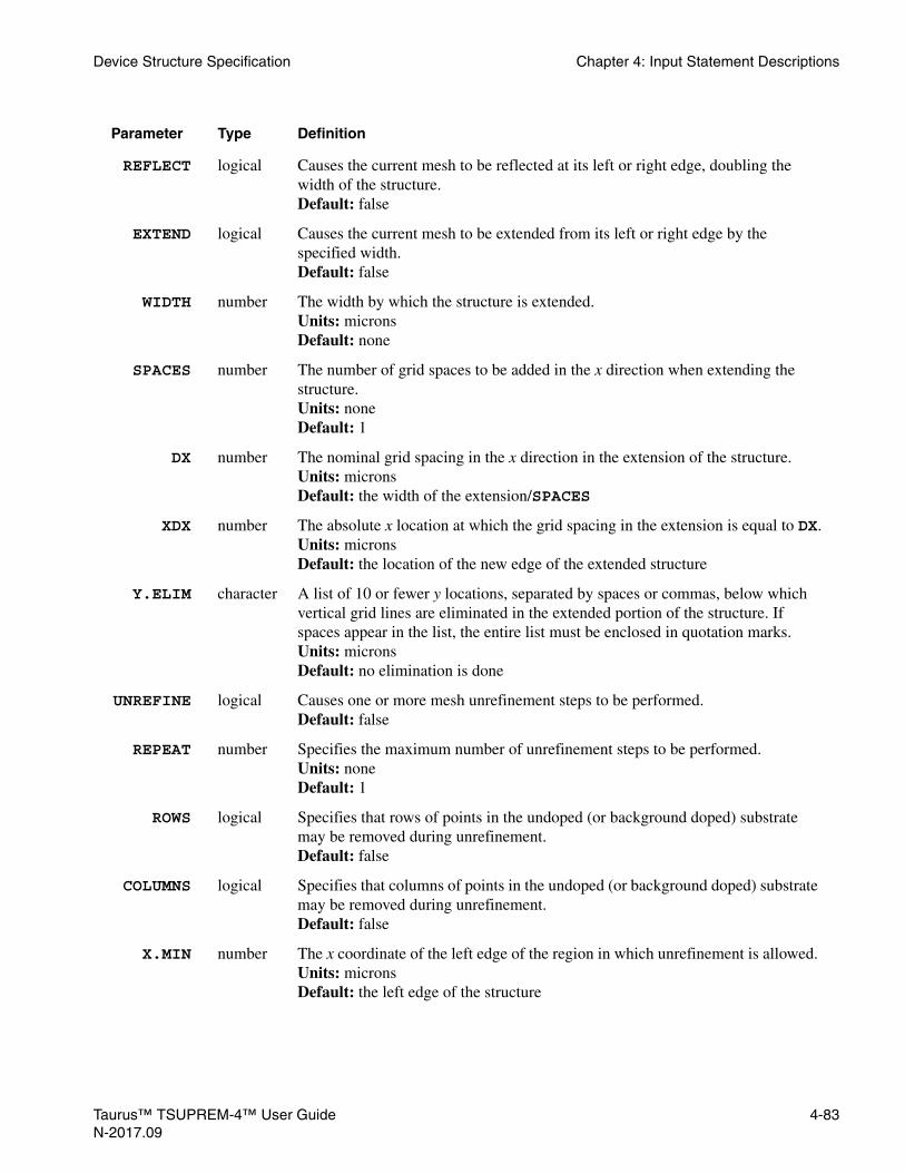
Device Structure Specification Chapter 4: Input Statement Descriptions

REFLECT logical Causes the current mesh to be reflected at its left or right edge, doubling the width of the structure.Default: false

EXTEND logical Causes the current mesh to be extended from its left or right edge by the specified width.Default: false

WIDTH number The width by which the structure is extended.Units: micronsDefault: none

SPACES number The number of grid spaces to be added in the x direction when extending the structure.Units: noneDefault: 1

DX number The nominal grid spacing in the x direction in the extension of the structure.Units: micronsDefault: the width of the extension/SPACES

XDX number The absolute x location at which the grid spacing in the extension is equal to DX.Units: micronsDefault: the location of the new edge of the extended structure

Y.ELIM character A list of 10 or fewer y locations, separated by spaces or commas, below which vertical grid lines are eliminated in the extended portion of the structure. If spaces appear in the list, the entire list must be enclosed in quotation marks.Units: micronsDefault: no elimination is done

UNREFINE logical Causes one or more mesh unrefinement steps to be performed.Default: false

REPEAT number Specifies the maximum number of unrefinement steps to be performed.Units: noneDefault: 1

ROWS logical Specifies that rows of points in the undoped (or background doped) substrate may be removed during unrefinement.Default: false

COLUMNS logical Specifies that columns of points in the undoped (or background doped) substrate may be removed during unrefinement.Default: false

X.MIN number The x coordinate of the left edge of the region in which unrefinement is allowed. Units: microns Default: the left edge of the structure

Parameter Type Definition

Taurus™ TSUPREM-4™ User Guide 4-83N-2017.09

Chapter 4: Input Statement Descriptions Device Structure Specification

Description The STRUCTURE statement is used to reflect, truncate, extend, or unrefine the current structure. The structure can be truncated on the left or right or at the bottom or top; reflected about its left or right edge, doubling its width; or extended from its left or right edge to the specified width. Truncation occurs before reflection, and reflection occurs before extension. Unrefinement occurs after truncation and extension. The last processing temperature can also be set for use in calculating active impurity concentrations for the SELECT or SAVEFILE statements.

Reflecting a structure also reflects any mask information associated with the structure. The mask information is truncated or extended (if necessary) to the value specified by X, then reflected.

The SPACES, DX, and XDX parameters specify the grid when a structure is extended. These parameters are used in the same way as the THICKNES, DY, and YDY parameters are used in the DEPOSITION and EPITAXY statements. The use of these parameters is described in Chapter 3, Changes to the Mesh During Processing, p. 3-7.

Note:The EXTEND feature should be used with caution. Simulating a narrow structure and then extending it does not give the same results as simulation of the wider structure unless the topography and doping concentrations at the edge of the narrow structure are essentially one-dimensional.

X.MAX number The x coordinate of the right edge of the region in which unrefinement is allowed. Units: microns Default: the right edge of the structure

Y.MIN number The y coordinate of the top of the region in which unrefinement is allowed. Units: microns Default: the top of the structure

Y.MAX number The y coordinate of the bottom of the region in which unrefinement is allowed. Units: microns Default: the bottom of the structure

TEMPERAT number Specifies the last processing temperature to be used for evaluating active impurity concentrations.Units: °Celsius Default: the last processing temperature specified, or 800°C

Parameter Type Definition

4-84 Taurus™ TSUPREM-4™ User GuideN-2017.09

Device Structure Specification Chapter 4: Input Statement Descriptions

Order ofOperations

The operations specified on the STRUCTURE statement are performed in the following order:

1. Set the last processing temperature, if specified with the TEMPERAT parameter.

2. Truncate the structure (if TRUNCATE is specified).

3. Reflect the structure (if REFLECT is specified).

4. Extend the structure (if EXTEND is specified).

5. Unrefine the structure (if UNREFINE is specified).

Usage Reflecting the structure about an edge that is not absolutely vertical can result in very thin triangles that could cause numerical problems. A structure should only be reflected about a reflecting boundary, created during an initial structure specification or by the TRUNCATE parameter.

TRUNCATE TOP can be used to remove the entire exposed surface, giving a structure with reflecting boundary conditions on all four sides. The usefulness of such structures is limited because some process steps (for example, DEPOSITION and ETCH) do not work on structures that have no exposed surface.

The UNREFINE parameter is used to remove unneeded mesh points from the structure. If REPEAT is more than 1, the unrefinement is repeated the specified number of times or until no further points can be removed. ROWS and COLUMNS allow removal of rows and columns of points in the undoped (or background doped) substrate. If both ROWS and COLUMNS are specified, rows and columns will be removed in alternating unrefinement steps. The X.MIN, X.MAX, Y.MIN, and Y.MAX parameters can be used to limit unrefinement to a portion of the structure.

TSUPREM-4Version

Compatibility

In versions of TSUPREM-4 before Version 5.1, the STRUCTURE statement is used to save and load structure files. Starting with Version 5.1, the SAVEFILE and LOADFILE statements should be used instead. Starting with Version 2000.2, the parameters for saving TSUPREM-4, Taurus Lithography, Medici, and minimos 5 files and for loading TSUPREM-4 and Taurus Lithography files are no longer accepted on the STRUCTURE statement.

Examples 1. The following statement truncates the structure to the right of x=1.2 microns, then mirrors the structure about the new right edge:

STRUCTURE TRUNCATE RIGHT X=1.2 REFLECT

2. The following statement extends the structure to the right by 0.5 microns. Two grid spaces are added, with elimination of every other vertical line below y=1 μm:

STRUCTURE EXTEND RIGHT WIDTH=0.5 SPACES=2 Y.ELIM=1.0

Taurus™ TSUPREM-4™ User Guide 4-85N-2017.09

Chapter 4: Input Statement Descriptions Device Structure Specification

3. The following statement causes up to four unrefinement steps to be performed:

STRUCTURE UNREFINE REPEAT=4 ROWS COLUMNS

The first and third steps allow rows of points to be removed in the substrate while the second and fourth steps allow columns to be removed.

4-86 Taurus™ TSUPREM-4™ User GuideN-2017.09

Device Structure Specification Chapter 4: Input Statement Descriptions

MASK

The MASK statement reads masking information from a file.

Description The MASK statement reads a file describing the mask levels used in a process. This mask information is used by the EXPOSE statement for patterning photoresist, which can be used as a masking layer for subsequent processing. By using mask files, the process description can be separated from the layout information, making it easy to simulate multiple layouts with a single process or multiple processes with a given layout.

The SCALE parameter specifies a scale factor to be applied to all dimensions and locations in the mask file.

The GRID and G.EXTENT parameters control how mask information is used to set the horizontal grid spacing during automatic grid generation. The GRID parameter specifies which mask levels are used. Fine grid spacing is used at the

MASK

[IN.FILE=<c>[SCALE=<n>][GRID=<c>][G.EXTENT=<c>]] [PRINT]

Parameter Type Definition

IN.FILE character Specifies a file containing mask information.Default: none

SCALE number Specifies a scale factor to be applied to all dimensions and locations in the mask file.Units: none Default: 1.0

GRID character One or more names of mask levels (separated by spaces or commas) for which fine horizontal grid is to be used during automatic grid generation.Default: all mask levels used

G.EXTENT character The distance that fine grid spacing extends under the lines on a mask. If a single value is specified, it is used for all mask levels specified with the GRID parameter (or all mask levels if GRID is not specified). If multiple values (separated by spaces or commas) are specified, then each value corresponds to a mask level specified with the GRID parameter. Negative values specify that fine grid extends into the spaces between the mask lines.Units: microns Default: 0.0

PRINT logical Prints mask information on the standard output and in the output listing file. The listing includes the names of all masks and the minimum and maximum x locations of each opaque segment of each mask.Default: false

Taurus™ TSUPREM-4™ User Guide 4-87N-2017.09

Chapter 4: Input Statement Descriptions Device Structure Specification

edges of lines on the specified levels. The G.EXTENT parameter determines how far the fine grid extends under the lines of the mask. The GRID and G.EXTENT parameters are character strings that specify lists of values; be sure to enclose them in quotation marks if they contain spaces.

TSUPREM-4 input mask files are created by Taurus Layout. Taurus Layout lets you view a mask layout file and interactively select regions to be simulated.

Examples 1. The following statement reads mask information from the file HVNCH.TL1 then prints the information that is read:

MASK IN.FILE=HVNCH.TL1 PRINT

2. The following statement specifies that only the POLY and FIELD masks should be considered when doing automatic grid generation. Fine grid should extend 0.5 microns under the edges of lines on the POLY mask and 0.3 microns under the edges of lines on the FIELD mask:

MASK IN.FILE=S4EX4M.TL1 GRID=”Poly,Field”+G.EXTENT="0.5,0.3"

3. TSUPREM-4 input files can be structured to separate the masking information from the processing information:

$ MESH DESCRIPTION (DEPENDS ON MASKS)LINE X LOC=0.0 SPAC=0.01...LINE Y LOC=200.0 SPAC=50.0INITIALIZE BORON=1E14$ MASK INFORMATIONMASK IN.FILE=MINNCH.TL1$ PROCESS INFORMATION (DOES NOT DEPEND ON MASKS)SOURCE CMOS07

To simulate a different portion of a layout with the same process, you only need to change the mesh description and the name of the MASK file. To simulate the same device with a modified process, you only need to change the name of the SOURCE file.

4-88 Taurus™ TSUPREM-4™ User GuideN-2017.09

Device Structure Specification Chapter 4: Input Statement Descriptions

PROFILE

The PROFILE statement allows a 1D impurity profile to be read from a file.

PROFILE

{ IMPURITY=<c> | ALL.IMP | ANTIMONY | ARSENIC | BORON |PHOSPHOR }

[MATERIAL=<c>][X.MIN=<n>] [X.MAX=<n>] [Y.MIN=<n>] [Y.MAX=<n>] [REPLACE] [EQ.RESET]{ IN.FILE=<c> [ZIP.FILE] [I.SCALE=<n>] [ { NM | UM | CM } ] { ( ONE.DIM [OFFSET=<n>] [SIGMA=<n>] )

|( TWO.DIM [X.OFFSET=<n>] [Y.OFFSET=<n>] [MIN.WT=<n>][I.SOURCE=<c>] [{ I.COLUMN=<c> | TIF | TS4 }])

} | EXPRESS=<c>}

Parameter Type Definition

IMPURITY character The name of the impurity for ONE.DIM or the name list of impurities for TWO.DIM to be read from the input file, or the impurity to be generated by the user-defined expression EXPRESS.Default: none

ALL.IMP logical Specifies to read all impurities from the IN.FILE file. Only applicable when the format of the IN.FILE file is in either TIF or TSUPREM-4 structure format.Default: false

ANTIMONY logical Specifies that the input file contains a profile of antimony concentration.Default: false Synonym: SB

ARSENIC logical Specifies that the input file contains a profile of arsenic concentration. Default: false Synonym: AS

BORON logical Specifies that the input file contains a profile of boron concentration. Default: false Synonym: B

PHOSPHOR logical Specifies that the input file contains a profile of phosphorus concentration. Default: false Synonym: P

MATERIAL character The name of the material into which data is to be imported. Only applicable for the import by TWO.DIM and EXPRESSDefault: silicon

Taurus™ TSUPREM-4™ User Guide 4-89N-2017.09

Chapter 4: Input Statement Descriptions Device Structure Specification

REPLACE logical Specifies that the profile read from the file should replace the existing profile (rather than adding to it).Default: false

EQ.RESET logical Specifies that the equilibrium state is automatically recalculated according to the change of solutions by importing the profiles.Default: true

X.MIN number Specifies the left boundary of the rectangular region into which the profile is imported.Units: microns or cm or nm, which is determined by UM or CM or NMDefault: leftmost location of the device

X.MAX number Specifies the right boundary of the rectangular region into which the profile is imported.Units: microns or cm or nm, which is determined by UM or CM or NMDefault: rightmost location of the device

Y.MIN number Specifies the top boundary of the rectangular region into which the profile is imported.Units: microns or cm or nm, which is determined by UM or CM or NMDefault: top location of the device

Y.MAX number Specifies the bottom boundary of the rectangular region into which the profile is imported.Units: microns or cm or nm, which is determined by UM or CM or NMDefault: bottom location of the device

IN.FILE character The name of the data file containing the 1D or 2D profile information. Default: none Synonym: INFILE

ZIP.FILE logical Specifies that the IN.FILE file is in compressed format.Default: false

I.SCALE character The list of the scaling number which corresponds to the list of impurities in the IMPURITY parameter. Scales the data when reading from the IN.FILE file.Default: 1 for one impurity, “1,1,1...” for multiple impurities

NM logical Specifies that the distance unit of data and the unit of X.MIN, X.MAX, Y.MIN, Y.MAX, OFFSET, X.OFFSET and Y.OFFSET are in nanometers.Default: false

UM logical Specifies that the distance unit of data and the unit of X.MIN, X.MAX, Y.MIN, Y.MAX, OFFSET, X.OFFSET and Y.OFFSET are in microns.Default: true

CM logical Specifies that the distance unit of data and the unit of X.MIN, X.MAX, Y.MIN, Y.MAX, OFFSET, X.OFFSET and Y.OFFSET are in centimeters.Default: false

ONE.DIM logical Specifies that the input file contains a 1D impurity profileDefault: true

Parameter Type Definition

4-90 Taurus™ TSUPREM-4™ User GuideN-2017.09

Device Structure Specification Chapter 4: Input Statement Descriptions

Description This statement allows a 1D impurity profile (or other solution variable) to be read from a data file. The data file must be a text file containing two columns of numbers. The first column gives the y coordinate of a point, in microns, and the second contains the impurity concentration (or other solution value), in

OFFSET number The amount by which the profile is shifted in the y-direction before being applied to the TSUPREM-4 structure. The concentration at y=0 in the data file is added at y=OFFSET in the TSUPREM-4 structure. Units: nanometers or microns or centimetersDefault: 0

SIGMA number Parameter of the erfc function, which is used for extrapolation of the profile outside of the specified rectangular regionUnits: microns

TWO.DIM logical Specifies that the input file contains a 2D impurity profile.Default: false

X.OFFSET number The amount by which the profile is shifted in the x-direction before being applied to the TSUPREM-4 structure. Only applicable for the 2D profile.Units: nanometers or microns or centimetersDefault: 0

Y.OFFSET number The amount by which the profile is shifted in the y-direction before being applied to the TSUPREM-4 structure. Only applicable for the 2D profile.Units: nanometers or microns or centimetersDefault: 0

MIN.WT number Minimum weight criteria not to discard the data out of material regions. Units: noneDefault: 0.001

I.SOURCE character The list of solution names to be read. Each name must correspond to the one in the IMPURITY list. The name must match exactly one in the IN.FILE file. Putting the character ‘-’ instead of a solution name automatically chooseS the proper name corresponding the IMPURITY name. Only applicable for TIF and TSUPREM-4 structure format files.Default: “-,-,-,...”

I.COLUMN character The column list which corresponds to the list of impurities in the IMPURITY parameter.Default: 3 for one impurity, “3,4,5...” for multiple impurities

TIF logical Specifies that the IN.FILE file format is TIF.Default: false

TS4 logical Specifies that the IN.FILE file format is TSUPREM-4 structure file format.Default: false

EXPRESS character The expression to generate the impurity profile to be imported.Default: none

Parameter Type Definition

Taurus™ TSUPREM-4™ User Guide 4-91N-2017.09

Chapter 4: Input Statement Descriptions Device Structure Specification

appropriate units. Lines in the data file that do not contain exactly two recognizable numeric values are ignored.

If REPLACE is specified, the profile read from the file replaces any existing profile. Replacement occurs only at nodes whose y coordinates are within the range of y coordinates given in the file. Adaptive gridding does not apply to the PROFILE statement. You must insure that the grid is dense enough to resolve the profile.

OFFSETParameter

The profile read from the data file is expanded in the x direction to the width of the structure and added to any existing impurities in the structure; negative data values can be used to reduce the concentration. The profile can be shifted in the y direction by specifying the OFFSET parameter. The profile is shifted by OFFSET, so that the concentration at y=0 in the data file appears at location y=OFFSET in the TSUPREM-4 structure.

Interpolation Values between the y coordinates specified in the input file are calculated using linear interpolation on the function

Equation 4-1

where:

• is the concentration in the file.

• is a scaling factor.

The final value of at each point is found by inverting using the value of obtained from the linear interpolation. This gives logarithmic interpolation for

and linear interpolation for . The value of is taken to be 105 for impurity and point defect concentrations and 1.0 for other solution variables (for example, dloop and rloop). At points outside the range of values in the input file, the impurity concentration remains unchanged.

IMPURITYParameter

The IMPURITY parameter can be used to read in values for a user-specified impurity. This can be used to read in a profile for comparison without altering the desired doping:

IMPLANT BORON ...SELECT Z=LOG10(BORON)PLOT.1D ...IMPURITY NEW IMPURITY=PBORONPROFILE IMPURITY=PBORON ...SELECT Z=LOG10(PBORON)PLOT.1D ^AX ^CL ...

If boron had been specified on the PROFILE statement, the profile would have been added to the implanted boron, making it impossible to compare the implanted profile with the contents of the data file.

f c( ) sign c( )logc

2k------

c2k------ 2

1++

=

c

k

c f c( ) f

c k» c k« k

4-92 Taurus™ TSUPREM-4™ User GuideN-2017.09

Device Structure Specification Chapter 4: Input Statement Descriptions

The IMPURITY parameter can be used to read in values of interstitial and vacancy profiles. Remember that the profiles read from the file are added to the profiles already in the structure, unless REPLACE is specified.

Profile in 2DRectangular

Region

Profile can be specified in 2D rectangular region inside the device. In this case impurity concentration is extrapolated by the erfc function outside the region:

,

where N(x) is initial 1D profile.

ImportingColumnwise 2D

Profiles

Two-dimensional impurity profiles, which are written in the following format, can be imported into the structure:

/x(um) y(um) C1(col=3) C2(col=4) C3(col=5) ... Cn0.0 0.1 1.2E21 3.8E19 8.4E17 ... 5.4E200.1 0.2 1.1E21 2.7E19 1.7E18 ... 9.2E19:

The line starting with a slash (/) is ignored. The first and second columns are always the x-axis and y-axis coordinates in microns, respectively. The data of the impurity species to be imported are defined by one of the following specifications:

• Either one of BORON, PHOSPHOR, ARSENIC, and ANTIMONY, or IMPURITY=impurity_name with the optional specification of I.COLUMN(default:3) when the data for one impurity are imported.

• IMPURITY="list_of_impurities" with the optional specification of I.COLUMN(default:“3,4,5...”) when the data of multiple impurities are imported.

The MATERIAL parameter (default: silicon) specifies the material region into which the data will be imported.

Note:The data that is located in the outside of the structure and the rectangle, (X.MIN,Y.MIN) and (X.MAX,Y.MAX), are ignored.

Importing 2DProfiles in TIF or

TS4 Format

• When I.SOURCE is specified, the names in the I.SOURCE list must be the exactly same names of the corresponding solutions in the file.

PROFILE TWO.DIM IN.FILE=test.tif TIF + IMPURITY=”arsenic,boron” I.SOURCE=”As,B”

• The character ‘-’ in the I.SOURCE list indicates to import the solution data which corresponds to the given impurity name:

PROFILE TWO.DIM IN.FILE=test.tif TIF + IMPURITY=”arsenic,boron” I.SOURCE=”-,B”

In the above example, the character ‘-’ means the TIF solution name “As” corresponding to arsenic. In addition, the B solution, which is the boron

N x y,( ) N x( )14--- erfc

x xmax–

σ-------------------- erfc

x xmin–

σ------------------- – erfc

y ymax–

σ-------------------- erfc

y ymin–

σ------------------- –=

Taurus™ TSUPREM-4™ User Guide 4-93N-2017.09

Chapter 4: Input Statement Descriptions Device Structure Specification

concentration in TIF, is to be added to boron solution into the current structure.

• When the value of the data to be imported is smaller than its minimum, which is either the hardwired internal value for the built-in solution (for example, 1E5 for boron) or the value defined with the parameter C.INIT for the user-defined impurity, it is set to the minimum value. However, when the solution has negative data, for example, SXX, the data must be imported as it is. Turning on the parameter NEGATIVE in the IMPURITY statement specifies that the impurity solution is allowed to have negative values. By default, it is turned on for all stress solutions, velocities, and the potential solution.

• The parameter EXPRESS lets you reset a solution whenever they want. For example,

PROFILE IMP=inters MAT=Si EXPR=1E22*exp(-y^2/0.1)

• You can reset a solution within a specific box region by setting X.MIN, X.MAX, Y.MIN and Y.MAX. You can reset multiple solutions at once:

PROFILE IMP="Sxx, Syy, Szz" MAT=Si EXPR=1E10 + X.MIN=0.1 X.MAX=0.2 Y.MIN=0 Y.MAX=0.1

• For TWO.DIM and EXPRESS imports, the equilibrium models associated with point-defects, such as point-defect pairing in PD.FULL, are recalculated automatically. Turning off EQ.RESET stops the equilibrium state from recalculating; this is not recommended.

Note:The PROFILE command does not import the model definition. Thus, you must set the proper model associated with the data to be imported before importing the data. For example, CL.FULL must be turned on before importing I2, I3, I4 solution data.

METHOD PD.FULL INTERST CL.FULLPROFILE TWO.DIM IN.FILE=test.tif TIF +

IMPURITY=”I2,I3,I4”

Examples • The following statement reads boron concentration data from the file bprof.dat:

PROFILE BORON IN.FILE=bprof.dat OFFSET=-0.1

If the file contained the lines:

0.0 1.0e170.1 1.4e170.2 1.8e170.4 2.0e170.6 1.8e170.8 1.4e171.0 1.0e172.0 1.0e165.0 1.0e14

4-94 Taurus™ TSUPREM-4™ User GuideN-2017.09

Device Structure Specification Chapter 4: Input Statement Descriptions

then a boron concentration of 1.0e17 would be added at y=-0.1, a concentration of 1.4e17 would be added at y=0, a concentration of 1.8e17 at y=0.1, and so on.

• The following statement defines boron profile in rectangular region.

PROFILE BORON IN.FILE=bprof.dat X.MIN=1 X.MAX=3 +Y.MIN=0.5 Y.MAX=3.5 SIGMA=0.01

• The following statement imports the 2D data of the third column for boron into the region of silicon material.

PROFILE TWO.DIM BORON IN.FILE=2dprof.dat

• The following statement imports the 2D data of the 5th column for indium into the region of polysilicon material.

PROFILE TWO.DIM IMP=INDIUM I.COLUMN=5 +IN.FILE=2dprof.dat

• The following statement imports the 2D data of the third and 5th columns for boron and arsenic respectively into the region of silicon material.

PROFILE TWO.DIM IMP=”BORON,ARSENIC” I.COL=”3,5” +IN.FILE=2dprof.dat

• The following statement imports the 2D data of the third column for arsenic into the region of silicon material only when the data is located in the inside of the rectangle, (0.5,0.0) and (1.0,2.0).

PROFILE TWO.DIM AS IN.FILE=2dprof.dat +X.MIN=0.5 Y.MIN=0.0 X.MAX=1.0 Y.MAX=2.0

• The following example shows that only arsenic, interstitial, and damage data among the data in test.tif is loaded into the default (silicon) material region. In addition, arsenic data is imported into oxide material region.

PROFILE TWO.DIM IN.FILE=test.tif TIF +IMPURITY="arsenic,interst,damage"

PROFILE TWO.DIM IN.FILE=test.tif TIF MAT=Ox + IMPURITY=arsenic

• The following example shows that the arsenic data is loaded within (left(=0.15um), top) and (right, bottom(=0.05um)) from test.sav which is written in TS4 structure format.

PROFILE TWO.DIM IN.FILE=test.sav TS4 IMP=arsenic +X.MIN=0.15 Y.MAX=0.05

• The following example shows that the boron data is loaded after shifting to the right by 0.03 um, downward by 0.02 um.

PROFILE TWO.DIM IN.FILE=test.tif TIF IMP=boron +X.OFFSET=0.03 Y.OFFSET=0.02

• The following example shows that the boron and arsenic data is scaled by 2 and 5, respectively, and loaded.

PROFILE TWO.DIM IN.FILE=test.tif TIF +IMPURITY="boron,arsenic" I.SCALE =" 2.0, 5.0"

Taurus™ TSUPREM-4™ User Guide 4-95N-2017.09

Chapter 4: Input Statement Descriptions Device Structure Specification

• The following statement imports the user-defined intermediate data AsImp and Iplus and adds them to arsenic and interstitial concentrations, respectively. The damage solution also is updated by adding the data from test.tif.

PROFILE TWO.DIM IN.FILE=test.tif TIF +IMPURITY="arsenic,interst,damage" +I.SOURCE=" AsImp, Iplus, -"

• There are two identical structures in equilibrium, but with different dopant distribution. When both structures need to be implanted with the same implant condition, the identical implantation on each structure must be performed. When the implantations are simulated by the MC implant model, using the PROFILE feature can remove the duplicated MC implant simulations. The example shows how to generate the arsenic profile of the MC implantation in such a case. The new impurity myAs is introduced because the implanted arsenic atoms must be separated from the background arsenic atoms.

• To calculate the +n interstitial profile, the current point-defect profiles are reset to their equilibrium concentrations by setting PD.FERMI followed by dummy diffusion for time=0. Then, the point-defect model is set to the 5-stream diffusion model to prevent the free interstitial concentration from being reduced by local equilibrium pairing. Since the implant adaptive gridding is internally applied by performing the analytic Taurus implantation first before the Monte Carlo implantation, TSUPREM-4 searches for the moment tables associated with myAs. Instead of manually creating the myAs moment tables by copying arsenic tables, the TIF name of the impurity myAs is temporarily assigned with As which is taken by Taurus analytic implant library for finding the analytic moment table for regrid. The simulation result is saved in TSUPREM-4 format so that the myAs data is stored in the name of the solution name myAs. However, if the simulation result is saved in TIF format, the TIF name of myAs should be different from As. Otherwise, the myAs data is saved in the name of its TIF name As which is also the arsenic’s TIF name, so the duplicated TIF names cause conflict.

$ The file for generating the MC implant profileIMPURIT NEW IMP=myAs DONOR AT.NUM=33.0 AT.WT=74.91INTERM NAME=Iplus EXPR=INTERST-CI.STAR

INITIAL IN.FILE=test1.tif TIF

METHOD PD.FERMIASSIGN NAME=tempC N.V=TEMP-273.16DIFFUSE TEMP=@tempC TIME=0

METHOD PD.5STRIMPURIT IMP=myAs TIF.NAME=AsIMPLANT IMP=myAs DOSE=1E15 ENERGY=30 TILT=30 +

MONTE N.ION=100000SAVEFIL OUT.FILE=mcimplant.str INTERMED ZIP

In the other input file, the arsenic profile is imported instead of simulating the MC implantation.

$ In other input files,$ instead of doing MC implant, importing the data

4-96 Taurus™ TSUPREM-4™ User GuideN-2017.09

Device Structure Specification Chapter 4: Input Statement Descriptions

$ IMPLANT ARSENIC DOSE=1E15 ENERGY=30 TILT=30 +$ N.ION=100000

PROFILE TWO.DIM IN.FILE=mcimplant.str TS4 ZIP +IMPURITY=”arsenic,inters,damage” +I.SOURCE=” myAs, Iplus,damage”

PROFILE TWO.DIM IN.FILE=mcimp.str TS4 ZIP MAT=Ox +IMPURITY=arsenic I.SOURCE=myAs

• When the transistors are formed in the epitaxy layer which was grown on the top of a silicon substrate, there is little flexibility in controlling the horizontal grids in the epitaxy layer because the horizontal grids in the epitaxy layer are determined by those of the underlying layer. The PROFILE statement provides the method to conveniently remesh the epitaxy region. Since the mesh is optimized to form the buried layer in the substrate region, the grid structure is not adequate for emitter, base, and collector which are formed near the top of the epitaxy layer. Thus, regridding is essential to efficiently and accurately simulate the bipolar process. After generating the new grid structure aimed to the formation of emitter, base, and collector, the solutions are imported to the new structure by the PROFILE statement. To import all solutions at once, the parameter ALL.IMP is turned on. After 0.2 um epitaxy growth, the top coordinate is -0.2 um. However, setting the top coordinate to zero might be more convenient for etching definition later. So Y.OFFSET is given to 0.2.

METHOD PD.FERMIPROFILE TWO.DIM IN.FILE=epi.tif TIF MAT=Si +

ALL.IMP Y.OFFSET=0.2

Taurus™ TSUPREM-4™ User Guide 4-97N-2017.09

Chapter 4: Input Statement Descriptions Device Structure Specification

ELECTRODE

The ELECTRODE statement is used to name the electrodes for device simulation.

Description The ELECTRODE statement allows you to specify names for electrodes. These electrode names are saved in TIF and MEDICI output files for use in Medici and other programs. The materials which can be named to an electrode are polysilicon and all materials which have been defined as conductors on a MATERIAL statement. Once an electrode is named, the information is kept unless it is undefined by CLEAR in an ELECTRODE statement.

ELECTRODE[NAME=<c>] [{ ( X=<n> [Y=<n>] ) | BOTTOM }][CLEAR [ALL]][MERGE][PRINT]

Parameter Type Definition

NAME character The name of the electrode to define or delete. This parameter is required unless both CLEAR and ALL are specified.Default: none

X number The x coordinate of an (x,y) position in the region to be defined as an electrode.Units: micronsDefault: none

Y number The y coordinate of an (x,y) position in the region to be defined as an electrode.Units: micronsDefault: the y coordinate inside the conductor at the x position

BOTTOM logical Specifies that the electrode to be defined is at the bottom of structure.Default: false

CLEAR logical Specifies that the named electrode is to be deleted.Default: false

MERGE logical Specifies the polysilicon adjacent to the electrode to be merged as the electrode.Only applicable to the saved file in TIF format.Default: true

ALL logical Specifies that all defined electrodes are to be deleted.Default: false

PRINT logical Specifies that the summary of defined electrodes is printed.Default: true

4-98 Taurus™ TSUPREM-4™ User GuideN-2017.09

Device Structure Specification Chapter 4: Input Statement Descriptions

Examples 1. The following statements show how to name the electrodes.

ELECTROD X=0.1 NAME=SourceELECTROD X=1.2 NAME=GateELECTROD X=2.3 NAME=DrainELECTROD BOTTOM NAME=BulkSAVEFILE OUT.FILE=mos.mdc MEDICI POLY.ELEELEC.BOT

2. The following statements show how to undefine the electrode.

ELECTROD X=0.1 NAME=Wrong...

ELECTROD NAME=Wrong CLEAR

AdditionalELECTRODE Notes

1. The polysilicon region named in ELECTROD is stored as an electrode in the saved file in TIF format. For Medici format, POLY.ELE must be specified in SAVEFILE.

2. The polysilicon region adjacent to the conductor named in ELECTROD is merged as the same electrode if MERGE parameter for TIF format, or POLY.ELE parameter (in SAVEFILE) for Medici format is specified.

3. If there are more than two conductors and/or polysilicon regions at the X position, for example, like EPROM structure, the Y must be specified individually.

ELECTROD X=1.2 Y=-0.02 NAME=EraseELECTROD X=1.2 Y=-0.35 NAME=Program

Taurus™ TSUPREM-4™ User Guide 4-99N-2017.09

Chapter 4: Input Statement Descriptions Process Steps

Process StepsThe following statements simulate processing steps:

Statement Name Description Page

DEPOSITION Deposits a material on the exposed surface. p. 4-101

EXPOSE Exposes photoresist using mask. p. 4-108

DEVELOP Removes exposed positive photoresist or unexposed negative photoresist.

p. 4-110

ETCH Etches an exposed material. p. 4-111

IMPLANT Implants an impurity. p. 4-117

DIFFUSION Performs a diffusion step, possibly with oxidation.

p. 4-136

EPITAXY Performs a silicon epitaxial deposition step. p. 4-142

STRESS Calculates the stresses in the structure. p. 4-147

4-100 Taurus™ TSUPREM-4™ User GuideN-2017.09

Process Steps Chapter 4: Input Statement Descriptions

DEPOSITION

The DEPOSITION statement is used to deposit a specified material on the exposed surface of the current structure.

DEPOSITION { MATERIAL=<c> | SILICON | OXIDE | OXYNITRI | NITRIDE

| POLYSILI | ALUMINUM| ( PHOTORES [ { POSITIVE | NEGATIVE } ] )

} [ IMPURITY=<c>

{ IT.CONC=<c> [IB.CONC=<c>] [LOG.GRAD] | I.PROFILE=<c> | I.RESIST=<n> } ]

[ANTIMONY=<n>] [ARSENIC=<n>] [BORON=<n>] [PHOSPHOR=<n>] [ {CONCENTR | RESISTIV} ] THICKNES=<n> [SPACES=<n>] [DY=<n>] [YDY=<n>] [ARC.SPAC=<n>]

[AR.MIN=<n>][TEMPERAT=<n>] [GSZ.LIN] [STRAINED][ANISOTRO=<n>] TOPOGRAP=<c>[RELAX]

Parameter Type Definition

MATERIAL character The name of the material to be deposited.Default: none

SILICON logical Deposit silicon. Default: false

OXIDE logical Deposit oxide. Default: false

OXYNITRI logical Deposit oxynitride. Default: false

NITRIDE logical Deposit nitride. Default: false

POLYSILI logical Deposit polysilicon. Default: false

ALUMINUM logical Deposit aluminum. Default: false

PHOTORES logical Deposit photoresist. Default: false

POSITIVE logical Specifies that the deposited photoresist (and all other photoresist in the structure) is positive, that is, that the DEVELOP statement removes exposed photoresist while leaving unexposed photoresist.Default: true, unless NEGATIVE is specified

Taurus™ TSUPREM-4™ User Guide 4-101N-2017.09

Chapter 4: Input Statement Descriptions Process Steps

NEGATIVE logical Specifies that the deposited photoresist (and all other photoresist in the structure) is negative, that is, that the DEVELOP statement removes unexposed photoresist while leaving exposed photoresist.Default: false

IMPURITY character The names of the impurities with which the deposited layer is doped. If there are several impurities provided, their names should be enclosed in quotes and separated by the commas.Default: none

IT.CONC character The concentrations of the specified impurities in the deposited layer. If there is only one impurity provided, then its concentration will be interpreted as a floating number. For several impurities, a list of their concentrations should be provided in the same order as the list of impurity names in the IMPURITY parameter. The list should be enclosed in quotes and the concentrations should be separated by the commas.Units: atoms/cm3

Default: noneSynonyms: I.CONC

IB.CONC character The impurity concentrations at the bottom of the deposited layer of the impurity species listed in the IMPURITY parameter. The impurity concentrations at the top of the layer must be specified by the IT.CONC parameter.Units: atoms/cm3

Default: Uniform impurity concentrations specified by IT.CONC

LOG.GRAD logical Specifies that the impurity concentrations specified by IMPURITY will vary logarithmically between the values specified by IB.CONC and IT.CONC.Default: false

I.PROFIL character The expression string for an equation that specifies the concentration of the single impurity specified by IMPURITY as a function of F, the fraction of the total layer thickness (or epitaxy time). F must obey the rules for a DEFINEd variable; it is recommended that it always by enclosed in braces and preceded by the "@" character; that is, it should always appear as "@{F}" in the equation.Units: atoms/cm3

Default: none

I.RESIST number The resistivity of the deposited layer.Units: ohm-cmDefault: none

ANTIMONY number The uniform concentration or resistivity of antimony in the deposited layer. Units: atoms/cm3 or ohm-cm Default: 0.0 Synonyms: SB

ARSENIC number The uniform concentration or resistivity of arsenic in the deposited layer.Units: atoms/cm3 or ohm-cm Default: 0.0 Synonym: AS

Parameter Type Definition

4-102 Taurus™ TSUPREM-4™ User GuideN-2017.09

Process Steps Chapter 4: Input Statement Descriptions

BORON number The uniform concentration or resistivity of boron in the deposited layer. Units: atoms/cm3 or ohm-cm Default: 0.0 Synonym: B

PHOSPHOR number The uniform concentration or resistivity of phosphorus in the deposited layer. Units: atoms/cm3 or ohm-cm Default: 0.0 Synonym: P

CONCENTR logical Specifies that the impurity concentration in the deposited layer is given. Default: true

RESISTIV logical Specifies that the resistivity in the deposited layer is given. Default: false

THICKNES number The thickness of the deposited layer. Units: microns Default: none

SPACES number The number of vertical grid spacings in the layer. This value is divided by the value of GRID.FAC (see MESH, p. 4-52).Units: noneDefault: 1/GRID.FAC Synonym: DIVISION

DY number The nominal grid spacing to be used in the deposited material layer at the location specified by the YDY parameter. This value is multiplied by the value of GRID.FAC (see MESH, p. 4-52).Units: microns Default: GRID.FAC*THICKNES/SPACES Synonym: DX

YDY number The location of the nominal grid spacing specified by DY relative to the top of the deposited layer. Units: microns Default: 0.0 Synonym: XDX

ARC.SPAC number The maximum spacing allowed along an arc on the new surface. This value is multiplied by the value of GRID.FAC (see MESH, p. 4-52).Units: microns Default: 0.5*THICKNES*GRID.FAC

AR.MIN number The minimum aspect (width/height) ratio for deposited grid spaces on planar surfaces.Default: 0.5

TEMPERAT number The deposition temperature; used to determine initial grain size when depositing polycrystalline materials.Units: °CelsiusDefault: 0.0

Parameter Type Definition

Taurus™ TSUPREM-4™ User Guide 4-103N-2017.09

Chapter 4: Input Statement Descriptions Process Steps

Description This statement provides a basic deposition capability. Material is deposited on the exposed surface of the structure, with the upper surface of the deposited layer becoming the new exposed surface. The ANTIMONY, ARSENIC, BORON, and PHOSPHOR parameters specify the initial impurity concentrations or resistivity in the deposited layer, depending on whether CONCENTR or RESISTIV is true. Doping can also be specified with the IMPURITY and I.CONC or I.RESIST parameters (see Specifying Initial Doping, p. 4-71).

The deposited material conforms to the contours of the original surface. Outside corners on the original surface produce arcs on the new surface, which are approximated by straight line segments. The maximum segment length is set by the ARC.SPAC parameter. The SPACES, DY, and YDY parameters used to control the grid spacing in the deposited layer are scaled by the value of the GRID.FAC parameter on the MESH statement (see Chapter 3, Changes to the Mesh During Processing, p. 3-7). The horizontal spacing in a thin deposited layer is the same as in the substrate, but for thick layers it is increased to avoid mesh elements with high ratios of height to width. This increase in horizontal spacing can be controlled with the AR.MIN parameter.

Note:It is not possible to deposit a layer on the bottom of a structure, even if it is exposed. Attempting to do so may cause the program to fail.

GSZ.LIN logical Specifies that the grain size increases linearly with depth from the bottom of the deposited layer. If false, the grain size is constant through the layer.Default: true

STRAINED logical Specifies whether the new SiGe or silicon layer is strained or relaxed.Default: false

ANISOTRO number Anisotropy of deposition, defined as a ratio of the layer thickness on top of a flat surface to the thickness of the layer deposited on a vertical wall. Anisotropy of 1 means isotropic deposition. Anisotropy of more than one means thinner layer on the sloped surface compared to the flat surface. Anisotropy can be any positive nonzero number. If it approaches infinity, then you get zero layer thickness on the vertical walls. If it approaches zero, then you are getting planarizing deposition filling everything up to the topmost point on the structure plus the nominal layer thickness.Default: 1

TOPOGRAP character The name of a file containing Taurus Topography input commands that define the deposition to be performed.Default: noneSynonym: TERRAIN

RELAX logical Specifies to perform the stress relaxation after depositionDefault: true

Parameter Type Definition

4-104 Taurus™ TSUPREM-4™ User GuideN-2017.09

Process Steps Chapter 4: Input Statement Descriptions

PolycrystallineMaterials

The TEMPERAT and GSZ.LIN parameters are used only when depositing a polycrystalline material. If no temperature is specified, or if the temperature is less than the value of TEMP.BRE for the material, the deposited layer is amorphous; recrystallization occurs at the start of the next high-temperature step.

Photoresist Photoresist can be positive or negative, but all photoresist in a structure must be of the same type. If photoresist of one type is deposited on a structure containing photoresist of the other type, a warning is issued and the type of the old photoresist is changed to that of the newly deposited photoresist.

Gradient-DopedDeposition

If IB.CONC is specified, the impurities named in the IMPURITY parameter will have the concentrations IB.CONC at the bottom of the deposited or grown layer and the concentrations IT.CONC at the top of the layer. The concentration will vary linearly through the layer unless LOG.GRAD is specified; in this case, the variation will be logarithmic. IB.CONC can only be used when IMPURITY and IT.CONC (alias I.CONC) are also specified.

If I.PROFIL is specified, it is interpreted as an equation specifying the concentration of a single impurity (specified by IMPURITY) as a function of F, the fraction of the layer thickness (F=0 at the bottom of the layer and F=1 at the top). The parameter F must obey the rules for a DEFINE variable; it is recommended that it be enclosed in braces and preceded by the "@" character, that is, "@{F}".

Note: The doping at interior nodes in the deposited layer is calculated by linear or logarithmic interpolation or by I.PROFIL. Thus, the total dose will be expected to differ from that calculated by analytical integration of the specified gradient (except in the special case of a linear gradient and a uniformly spaced grid).

Deposition WithTaurus

Topography

The TOPOGRAP parameter invokes Taurus Topography with the specified command input file. The command input file contains Taurus Topography commands describing one or more processing steps to be simulated by Taurus Topography. It should not contain the INITIALIZE or STOP statements.

The values of variables set with the ASSIGN, DEFINE, and EXTRACT statements are substituted in the Taurus Topography command input file. In addition to variables set explicitly by you, if the THICKNES parameter is set on the DEPOSITION statement, then its value is assigned to the variable THICK before substitution. (If the variable THICK is assigned in this way, it will be unset after the DEPOSITION statement, even if it was set by you previously.) This allows parameter values (such as deposition thickness) to be passed to Taurus Topography. The most recent mask file specified in the TSUPREM-4 input file is passed to Taurus Topography for use in masked etch steps.

By default, Taurus Topography is called by requesting that the command TOPOGRAPHY be executed by the operating system, but if the environment

Taurus™ TSUPREM-4™ User Guide 4-105N-2017.09

Chapter 4: Input Statement Descriptions Process Steps

variable S4TERRAIN is set, its value is used instead. It may be necessary for you to define other environment variables (for example, TERR_LIB) for Taurus Topography to run correctly. For additional details, refer to the Taurus Topography Reference Manual.

When Taurus Topography is invoked with the DEPOSITION statement, the full set of parameters is used for any deposited layer of the specified material. Thus you have full control over grid spacing, doping, and polycrystalline grain size. Note that the parameters specified on the DEPOSITION statement only apply to the specified material. They are ignored for other materials deposited by Taurus Topography.

Examples 1. The following statement deposits 200 angstroms of silicon dioxide:

DEPOSIT OXIDE THICK=0.02

2. The following statement deposits a one-micron thick layer of photoresist, using four grid spaces in the layer:

DEPOSIT PHOTO THICK=1.0 SPACES=4 ARC.SPAC=0.1

The maximum segment length used to approximate arcs is 0.1 micron. By default, the newly deposited photoresist (and any photoresist already present in the structure) is assumed to be positive.

3. The following statement deposits 0.1 micron of poly:

DEPOSIT MAT=POLY THICK=0.1 TEMPERAT=650 GSZ.LIN

The initial grain size is calculated at 650× ° C, and increases linearly over the thickness of the layer, with minimum value at the bottom of the layer.

4. The following statement calls Taurus Topography with the input command file PolyDep.inp:

DEPOSIT MAT=POLY THICK=0.1 TEMPERAT=650 GSZ.LIN +TOPOGRAPHY=PolyDep.inp

References to “@THICK” in the Taurus Topography input file are replaced with the value “0.1”. If the call to Taurus Topography causes the deposition of a polysilicon layer, then the specified temperature and grain size model are used for that layer.

5. The following statement deposits a strained SiGe layer:

DEPOSIT STRAINED SILICON THICKNES=0.1 SPAC=15 +IMPURITY=germanium I.CONC=2.5e21

6. Silicon deposition with Ge that varies from 10% (bottom) to 20% (top):

DEPOSIT SILICON THICKNES=0.1 SPACES=10 +IMP=GERMANIUM I.CONC=1E22 IB.CONC=0.5E22

7. Same as 6. But use I.PROFILE.

DEPOSIT SILICON THICKNES=0.1 SPACES=10 +IMP=GERMANIUM +I.PROFIL=( 0.5E22 + @{F}*(1E22-0.5E22) )

4-106 Taurus™ TSUPREM-4™ User GuideN-2017.09

Process Steps Chapter 4: Input Statement Descriptions

8. Deposition with linear gradient multiple species:

DEPOSIT POLY THICK=0.2 SPACES=10 TEMP=800 GSZ.LIN +IMP="BORON, PHOSPHORUS" +IB.CONC="5E13 1E15" +I.CONC="5E14 2E15"

AdditionalDEPOSITION

Notes

1. The calculation doping concentration from resistivity uses mobility tables for silicon and polysilicon. If the resistivity is specified when depositing some other material, a warning is issued. The mobility tables used for calculating the doping concentration are not the same as the tables used by the ELECTRICAL statement. The extracted sheet resistance for the deposited layer does not correspond exactly to the resistivity specified during deposition.

2. Deposition of one material on top of another can cause a third material to be added between them. This happens when titanium is deposited on silicon, for example—a layer of TiSi2 is inserted. Insertion of extra layers is specified with the REACTION statement (see p. 4-308).

3. Diffusion of impurities during a deposition step is not simulated, even though a temperature may be specified.

Taurus™ TSUPREM-4™ User Guide 4-107N-2017.09

Chapter 4: Input Statement Descriptions Process Steps

EXPOSE

The EXPOSE statement exposes photoresist using a mask.

EXPOSE

MASK=<c>[SHRINK=<n>][OFFSET=<n>]

Description The EXPOSE statement exposes photoresist, using masking information previously read with a MASK statement. Regions of photoresist that are directly below transparent regions of the specified mask (and not obscured by any other material) are marked as exposed. If positive photoresist is present, exposed regions are removed by a subsequent DEVELOP statement; if negative photoresist is present, the unexposed portion of the photoresist is removed.

The SHRINK and OFFSET parameters can be used to model the effects of deliberate or accidental adjustments to the mask-making or photolithographic processes. SHRINK specifies a reduction in the width of lines on the mask, while OFFSET specifies a shifting of the mask (relative to other masks). The program does not allow shrinks or offsets that are large enough to make mask lines or spaces disappear.

Note:The OFFSET parameter breaks the symmetry that is assumed at reflecting boundaries at the edge of a structure. Shifting a line towards a reflecting boundary also makes it narrower, while shifting a line away from a reflecting boundary makes it wider.

Parameter Type Definition

MASK character Specifies the name of the mask to be used for the exposure step. The mask name must match the name of a mask previously read with a MASK statement.Default: none

SHRINK number The reduction in line width on each side of each line on the mask. The total reduction in line width is twice the specified value.Units: micronsDefault: 0.0

OFFSET number The amount by which lines on the mask are shifted (in the positive x direction).Units: micronsDefault: 0.0

4-108 Taurus™ TSUPREM-4™ User GuideN-2017.09

Process Steps Chapter 4: Input Statement Descriptions

Example The following sequence illustrates a typical use of the EXPOSE statement:

MASK IN.FILE=CMOS3.TL1...DEPOSIT POLY THICKNES=.2DEPOSIT POSITIVE PHOTORES THICKNES=1EXPOSE MASK=POLY SHRINK=0.05DEVELOPETCH POLY TRAP THICK=0.4 ANGLE=80ETCH PHOTORES ALL

This sequence produces lines of polycrystalline silicon under the opaque regions of the mask named POLY. The width of each POLY line is reduced by 0.05 microns on each side (for a total reduction of 0.1 micron).

Taurus™ TSUPREM-4™ User Guide 4-109N-2017.09

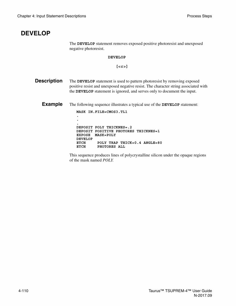
Chapter 4: Input Statement Descriptions Process Steps

DEVELOP

The DEVELOP statement removes exposed positive photoresist and unexposed negative photoresist.

Description The DEVELOP statement is used to pattern photoresist by removing exposed positive resist and unexposed negative resist. The character string associated with the DEVELOP statement is ignored, and serves only to document the input.

Example The following sequence illustrates a typical use of the DEVELOP statement:

MASK IN.FILE=CMOS3.TL1...DEPOSIT POLY THICKNES=.2DEPOSIT POSITIVE PHOTORES THICKNES=1EXPOSE MASK=POLYDEVELOPETCH POLY TRAP THICK=0.4 ANGLE=80ETCH PHOTORES ALL

This sequence produces lines of polycrystalline silicon under the opaque regions of the mask named POLY.

DEVELOP

[<c>]

4-110 Taurus™ TSUPREM-4™ User GuideN-2017.09

Process Steps Chapter 4: Input Statement Descriptions

ETCH

The ETCH statement is used to remove portions of the current structure.

ETCH [ { MATERIAL=<c> | SILICON | OXIDE | OXYNITRI | NITRIDE | POLYSILI | PHOTORES | ALUMINUM } ] { ( TRAPEZOI [THICKNES=<n>] [ANGLE=<n>] [UNDERCUT=<n>] ) | ( {LEFT | RIGHT} [P1.X=<n>] [P1.Y=<n>] [P2.X=<n>] [P2.Y=<n>] ) | ( {START | CONTINUE | DONE} X=<n> Y=<n> )

| (ISOTROPI [MULT.ETC=<n>] ) | ( OLD.DRY THICKNES=<n> ) | ALL

| TOPOGRAP=<c> }

[RELAX]

Parameter Type Definition

MATERIAL character The name of the material to be etched.Default: none

SILICON logical Etch silicon only. Default: false

OXIDE logical Etch oxide only. Default: false

OXYNITRI logical Etch oxynitride only. Default: false

NITRIDE logical Etch nitride only. Default: false

POLYSILI logical Etch polysilicon only. Default: false

PHOTORES logical Etch photoresist only. Default: false

ALUMINUM logical Etch aluminum only. Default: false

TRAPEZOI logical Use an etch model that removes material from a trapezoidal region when applied to a planar surface. This is a generalization of the DRY model in older versions of TSUPREM-4.Default: trueSynonym: DRY

Taurus™ TSUPREM-4™ User Guide 4-111N-2017.09

Chapter 4: Input Statement Descriptions Process Steps

THICKNES number The thickness of the layer to be removed when the TRAPEZOI or OLD.DRY parameter is specified. Units: microns Default: UNDERCUT*tan(ANGLE) for ANGLE<90, infinite otherwise; no default if OLD.DRY is specified

ANGLE number The angle of the sidewalls produced when the TRAPEZOI parameter is specified. The angle is measured from the horizontal, so that vertical sidewalls have an angle of 90 deg.Units: degreesDefault: arctan(THICKNES/UNDERCUT) if THICKNES and undercut are both specified, 90 otherwise

UNDERCUT number The distance that the etch extends under masking layers when the TRAPEZOI parameter is specified. Units: microns Default: THICKNES/tan(ANGLE) for ANGLE<90, 0 otherwise

LEFT logical Etch material to the left of the specified position. Default: false

RIGHT logical Etch material to the right of the specified position. Default: false

P1.X number The x coordinate of the first point used when LEFT or RIGHT is specified. Units: microns Default: 0.0

P1.Y number The y coordinate of the first point used when LEFT or RIGHT is specified. Units: microns Default: a point above the top of the structure

P2.X number The x coordinate of the second point used when LEFT or RIGHT is specified. Units: microns Default: the value of P1.X

P2.Y number The y coordinate of the second point used when LEFT or RIGHT is specified. Units: microns Default: a point below the bottom of the structure

START logical The point (X,Y) is the first point in a series defining the region to be etched. Default: false

CONTINUE logical The point (X,Y) is the next point in a series defining the region to be etched. Default: false

DONE logical The point (X,Y) is the last point in a series defining the region to be etched. Default: false Synonym: END

ISOTROPI logical Specifies removal of material that lies within THICKNES of an exposed surface.Default: false

Parameter Type Definition

4-112 Taurus™ TSUPREM-4™ User GuideN-2017.09

Process Steps Chapter 4: Input Statement Descriptions

Description This statement is used to remove a portion of the current structure. You can define the region to be removed and optionally specify a material to be removed; if no material is specified, all materials are considered to be etchable. Portions of the structure are removed, provided that they are of an etchable material, lie within the defined etch region, and are exposed to the ambient. See Chapter 3, Etching, p. 3-175 for a more complete description. The surface under the etched portions of the structure is marked as exposed. The warning:

*** Warning: No material removed by ETCH statement.

is produced by an attempt to etch a material that is not exposed, or by specifying etch coordinates that do not include any etchable material.

RemovingRegions

You can specify the region to be removed in one of the following ways:

1. If TRAPEZOI is specified, the etch region is found from a simple model of a primarily anisotropic (that is, vertical, or directional) etch with a small isotropic component. This model can produce profiles with sloped sidewalls and undercutting of masking layers. See Chapter 3, Trapezoidal Etch Model, p. 3-176.

MULT.ETC number Specifies that an isotropic etch step is to be performed by MULT.ETC-steps instead of one step.Units: noneDefault: 1Synonym: MULTETCH

X number The x coordinate used with the START, CONTINUE, or DONE parameter.Units: microns Default: none

Y number The y coordinate used with the START, CONTINUE, or DONE parameter. Units: microns Default: none

OLD.DRY logical The exposed surface is etched vertically by an amount given by the THICKNES parameter. Default: false

ALL logical The specified material is etched away entirely. Default: false

TOPOGRAP character The name of a file containing Taurus Topography input commands that define the etch to be performed.Default: noneSynonym: TERRAIN

RELAX logical Specifies to perform the stress relaxation after etchDefault: true

Parameter Type Definition

Taurus™ TSUPREM-4™ User Guide 4-113N-2017.09

Chapter 4: Input Statement Descriptions Process Steps

2. If LEFT or RIGHT is specified, the etch region includes all material to the left or right of the line between (P1.X,P1.Y) and (P2.X,P2.Y).

3. The START, CONTINUE, and DONE parameters are used with the X and Y parameters to define arbitrarily complex etch regions. The boundary of the region is determined by a series of ETCH statements, each specifying a point on the boundary. The first statement of the series should contain the START parameter, the last should contain the DONE parameter, and statements in between should use the CONTINUE parameter. The last point is connected to the first point to produce a closed region defining the portion of the structure to be removed.

4. If ISOTROPI is specified, the etch region includes all material within the distance THICKNES of the exposed surface. This produces a simple isotropic etch, without rounding of outside corners. Since the isotropic etch region is instantly defined by the etch boundary where the normal distance to the exposed surface is an etch thickness, the mask layer does not work correctly when the etch thickness exceeds the mask layer thickness. In the following structure shown in the left side of the figure which has a 0.2-um thick mask layer with a 0.1-um open window on the top of silicon substrate, each different color dot line shows each segmented isotropic etch boundary with 0.25-um thickness. Consequently, the result of the 0.25-um isotropic etch is shown in the right side of the figure where the mask layers are detached and removed. Replacing a thick single etch step with thin multiple etch steps can avoid this problem if the individual thickness of the multiple etch steps is thinner than the minimum thickness of the mask layer. The parameter MULT.ETC in the METHOD or ETCH statements specifies that an isotropic etch step is to be performed by MULT.ETC-steps instead of one step. The etched thickness of each step is THICKNES/MULT.ETC. The stress relaxation is performed at the final step of the multiple etch steps if RELAX is turned on.

4-114 Taurus™ TSUPREM-4™ User GuideN-2017.09

Process Steps Chapter 4: Input Statement Descriptions

5. If the OLD.DRY parameter is specified, the etch region includes all material within a vertical distance THICKNES of the exposed surface. This model (the DRY model in previous versions of TSUPREM-4) has been replaced by the TRAPEZOI model.

The OLD.DRY model in Version 5.1 of TSUPREM-4 is the same as the DRY model in older versions of the program. In Version 5.1, DRY is a synonym for TRAPEZOI. The TRAPEZOI model with default values of ANGLE and UNDERCUT is equivalent to the OLD.DRY model, except that surface layers of nonetchable material blocks etching of underlying material, even if the surface layer is thinner than THICKNES. Specifying DRY in Version 5.1 is equivalent to specifying DRY in previous versions in cases of practical interest.

6. If the ALL parameter is specified, the etch region includes the entire structure.

• If no region specification is given, TRAPEZOI is assumed.

• If a material is specified, only that material is etched; otherwise, the entire region specified is subject to removal.

It is possible to cut the structure into two or more pieces with an ETCH statement. In this case, all pieces except the one with the largest area are removed. A warning is issued for each piece removed.

Note:The ETCH statement (except when used with the TERRAIN parameter) is not intended to simulate a physical etching process; its purpose is to provide a means to generate the required structures for simulation of diffusion and oxidation. Note in particular that the statement “ETCH OXIDE TRAP” does not implement a selective etch of oxide, but rather defines a region geometrically in which all exposed oxide is removed.

Etching WithTaurus

Topography

The TOPOGRAP parameter invokes Taurus Topography with the specified command input file. The command input file contains Taurus Topography commands describing one or more processing steps to be simulated by Taurus Topography. It should not contain the INITIALIZE or STOP statements.

The values of variables set with the ASSIGN, DEFINE, and EXTRACT statements are substituted in the Taurus Topography command input file. In addition to variables set explicitly by you, if the THICKNES parameter is set on the ETCH statement, then its value is assigned to the variable THICK prior to substitution. (If the variable THICK is assigned in this way, it will be unset after the ETCH statement, even if it was set by you previously.) This allows parameter values (such as etch thickness) to be passed to Taurus Topography. The most recent mask file specified in the TSUPREM-4 input file is passed to Taurus Topography for use in masked etch steps.

By default, Taurus Topography is called by requesting that the command topography be executed by the operating system, but if the environment variable S4TERRAIN is set, its value is used instead.

Taurus™ TSUPREM-4™ User Guide 4-115N-2017.09

Chapter 4: Input Statement Descriptions Process Steps

It may be necessary for you to define other environment variables (for example, TERR_LIB) for Taurus Topography to run correctly. For additional details, refer to the Taurus Topography Reference Manual.

Examples 1. The following statement etches the nitride to the left of 0.5 μm to a depth of 1 micron:

ETCH NITRIDE LEFT P1.X=0.5 P2.Y=-1.0

Note:P1.Y defaults to a location above the top of the structure and P2.X defaults to the value of P1.X (that is, 0.5).

2. This statement etches the oxide in the square defined by (0,0), (1,0), (1,1), (0,1):

ETCH OXIDE START X=0.0 Y=0.0ETCH CONTINUE X=1.0 Y=0.0ETCH CONTINUE X=1.0 Y=1.0ETCH DONE X=0.0 Y=1.0

Material is removed only if there is an exposed oxide surface somewhere within the boundaries of the etch.

3. The following statement calls Taurus Topography with the input command file PolyDep.inp:

ETCH THICK=0.1 TOPOGRAPHY=PolyDep.inp

References to “@THICK” in the Taurus Topography input file are replaced with the value “0.1”.

4. The following statement etches all materials except silicon:

ETCH ^SILICON ALL

4-116 Taurus™ TSUPREM-4™ User GuideN-2017.09

Process Steps Chapter 4: Input Statement Descriptions

IMPLANT

The IMPLANT statement is used to simulate the ion implantation of impurities into the structure.

IMPLANT

{IMPURITY=<c> | ANTIMONY | ARSENIC | BORON | ( BF2 [MOLECULE] ) | PHOSPHOR}DOSE=<n> ENERGY=<n> [TILT=<n>] [ROTATION=<n>] [MULT.ROT=<n>][{EXTEND | PERIODIC | REFLECT | VACUUM}] [MARGIN=<n>] [DAMAGE] [D.PLUS=<n> | D.P1=<n>] [D.SCALE=<n>] [D.RECOMB][L.RADIUS=<n> { (L.DENS=<n> [L.DMIN=<n>] [L.DMAX=<n>])

| (L.THRESH=<n> [L.FRAC=<n>]) }][REGRID] [PAI] [DOSE.SCA]{ ( [{GAUSSIAN | PEARSON}] [BACKSACT] [PAI.THRE=<n>]

[IMPL.TAB=<c>] [DAM.TABL=<c>] [DAM.FILE=<c>] [MOMENTS] [ALSO.TAB] [PRINT] [DAM.ADAP] [GE.EFF]

[V.PLUS=<n>] [DX.FP=<n>] [DY.FP=<n>] [DX.IPLUS=<n>] [DY.IPLUS=<n>]{ ([RP.EFF] [IN.FILE=<c>] [OXTH.FAC=<n>])| ([DATA.SUF=<c>] [DAM.SUF=<c>] [DATA.PAT=<c>] [RANGE.SH=<n>])}

)| ( [N.ION=<n>] [BEAMWIDT=<n>] [SEED=<n>] [CRYSTAL] [TEMPERAT=<n>]

{ MONTECAR [DAM.MOD=<c>] [DEPTH.SP] [DOSE.SPL] [TRAJ.SPL] [TRAJ.REP][X.INTERV=<n>] [REC.OXYG] [RANDOM] [POINT.RE] [MAX.SPLI][SAVE1D [SAVE1D.F=<c>] [SAVE1D.S] [SAVE1D.H] [SAVE1D.U=<c>]]

| OLD.MC [VIBRATIO [X.RMS=<n>] [E.LIMIT=<n>]][THRESHOL=<n>] [POLY.GSZ=<n>] [INTERST=<c>] [MAX.DAM=<n>][REC.FRAC=<n>] [CRIT.PRE] [CRIT.F] [CRIT.110]

})

}[SAVEFILE=<c>] [ {LOADFILE=<c> [LOAD.WT=<n>]} ] [ZIP.FILE]

Parameter Type Definition

IMPURITY character The name of the impurity to be implanted.Default: noneSynonym: IMP

ANTIMONY logical Specifies that antimony is to be implanted. Default: false Synonym: SB

ARSENIC logical Specifies that arsenic is to be implanted. Default: false Synonym: AS

Taurus™ TSUPREM-4™ User Guide 4-117N-2017.09

Chapter 4: Input Statement Descriptions Process Steps

BORON logical Specifies that boron is to be implanted. Default: false Synonym: B

BF2 logical Specifies that boron in the form of BF2 is to be implanted. Default: false

MOLECULE logical Specifies that fluorine is to be implanted when BF2 is implanted. Applies to BF2 only.Default: false

PHOSPHOR logical Specifies that phosphorus is to be implanted. Default: false Synonym: P

DOSE number The dose of implanted ions. Units: atoms/cm2 Default: none

ENERGY number The acceleration energy of the ion implant beam. Units: keV Default: none

TILT number Specifies the tilt angle of the wafer, measured in a clockwise direction from the horizontal in the plane of the simulation. Positive tilt angles correspond to implanted ions arriving from the left side of vertical, and negative tilt angles correspond to implanted ions arriving from the right side of vertical (assuming the wafer rotation angle is less than 90 degrees and greater than –90 degrees). Tilting of the wafer with respect to the ion beam can contribute to shadowing, dose reduction and foreshortening of the implant distribution; see Chapter 3, Analytic Ion Implant Models, p. 3-135.Units: degreesDefault: 0

ROTATION number The angle by which the ion beam has been rotated from the [110] primary flat orientation, measured in a clockwise direction about an axis perpendicular to and facing into the wafer surface. Implanting with a value of 0.0 for this parameter corresponds to implantation in the plane formed by Y-axis and [110] flat direction. Wafer rotation can contribute to shadowing of portions of the simulation structure (see Chapter 3, Analytic Ion Implant Models, p. 3-135).Units: degrees Default: 0

MULT.ROT number The number of rotations by the rotational angle 360 deg/MULT.ROT degrees with the starting angle ROTATION.Default: 1

EXTEND logical Specifies that extend (1D-continuation) boundary conditions be imposed at the left and right edges of the structure during implantation. Applies to the Taurus analytic and Taurus MC models only.Default: true

Parameter Type Definition

4-118 Taurus™ TSUPREM-4™ User GuideN-2017.09

Process Steps Chapter 4: Input Statement Descriptions

PERIODIC logical Specifies that periodic boundary conditions be imposed at the left and right edges of the structure during implantation. Applies to the Taurus analytic and all MC models.Default: false

REFLECT logical Specifies that reflecting boundary conditions be imposed at the left and right edges of the structure during implantation. Applies to the Taurus analytic and all MC models.Default: false

VACUUM logical Specifies that boundary conditions corresponding to vacuum material be imposed at the left and right edges of the structure during MC implantation. Applies to the Taurus analytic and all MC models.Default: false

MARGIN number Specifies the size of the margins by which the simulation domain is expanded during implantation to account for the boundary conditions. Applies to the Taurus analytic and Taurus MC models only.Default: automatically determined.

DAMAGE logical Specifies that point defects generated by ion implantation are to be retained and used as an initial condition for subsequent process steps. Default: true when PD.TRANS or PD.FULL is selected

D.PLUS number The scale factor applied to the implanted profile to obtain the plus one component of the damage profile.Units: none Default: effective +n model used

D.P1 number The +1 component of the effective +n model for implant damage.Units: none Default: 1.0

D.SCALE number The scale factor applied to the Frenkel pair component of the damage profile.Units: none Default: 1.0

D.RECOMB logical Compute the recombination of interstitials and vacancies analytically at the end of the IMPLANT step.Default: true

L.RADIUS number The radius of dislocation loops (if any) resulting from the implant. Units: cmDefault: none

L.DENS number The density of dislocation loops (if any) resulting from the implant. Units: #/cm3

Default: none

Parameter Type Definition

Taurus™ TSUPREM-4™ User Guide 4-119N-2017.09

Chapter 4: Input Statement Descriptions Process Steps

L.DMIN number The minimum damage level used to define the region where dislocation loops are produced.Units: #/cm3

Default: 1e20

L.DMAX number The maximum damage level used to define the region where dislocation loops are produced.Units: #/cm3Default: 1.15e22

L.THRESH number The interstitial concentration above which dislocation loops are produced. Units: #/cm3Default: none

L.FRAC number The fraction of interstitials in excess of L.THRESH that are incorporated into dislocation loops.Units: noneDefault: 1.0

REGRID logical If true, the mesh is adoptively regridded using Taurus analytic implant for library-based Taurus MC implant. Synonym: TS4.REGRDefault: true

PAI logical Taurus implant parameter (PAI). Determines if the pre-existing implant damage should be taken into account during the implantation. Applies to the Taurus analytic and Taurus MC models only.Default: true

DOSE.SCA logical Enables the nominal implant dose integration along the direction of wafer normal. When it is false, the nominal dose is the value integrated along the ion beam direction. Applies to the Taurus analytic and Taurus MC models only.Default: false

GAUSSIAN logical Specifies that a simple Gaussian distribution is to be used to represent the implanted impurity profile. Default: false

PEARSON logical Specifies that a Pearson or dual-Pearson distribution is to be used to represent the implanted impurity profile. Default: true, unless GAUSSIAN is specified

BACKSCAT logical Enables modeling of backscattering of ions from the surface.Default: true

PAI.THRE number Threshold implant damage concentration for the conversion of the implant damage into an equivalent amorphous layer thickness. Applies to the Taurus analytic model onlyUnits: cm-3Default: 2.5e22

Parameter Type Definition

4-120 Taurus™ TSUPREM-4™ User GuideN-2017.09

Process Steps Chapter 4: Input Statement Descriptions

IMPL.TAB character The name used to choose the range statistics from the implant moment data file. Default: antimony, tr.indium, dual.ars, chboron, dual.bf2, and dual.pho for ANTIMONY, INDIUM, ARSENIC, BORON, BF2, and PHOSPHOR implantations, respectively. Use IMPL.TAB=taurus to select the Taurus Analytic Implant Model.Synonym: NAME

DAM.TABL character The name of a table of damage parameters in an implant damage file. Values of the RANGE, SIGMA, LAMBDA, LSIGMA, LSLOPE, and SCALE parameters for implant damage are taken from the specified table in the implant damage file (unless specified on a preceding MOMENT statement).Default: If DAM.TABL is not specified on the IMPLANT statement, a table name specified on an IMPURITY statement is used or parameters are obtained from the built-in equations

DAM.FILE character The name of a file continuing tables of damage parameters.Default: The file specified by the environment variable S4IDAM or the file named “s4idam” in the current working directory.

MOMENTS logical Use range statistics from previously specified MOMENT statements, instead of from a moment data file.Default: false

ALSO.TAB logical This parameter is only valid when paired with MOMENTS. Enables TSUPREM-4 to get the missing moments from the implant tables if necessary. The implant table for silicon could be specified using IMPL.TAB keyword. If IMPL.TAB is not specified, the default table is used.Default: false

PRINT logical Prints a summary of the current implantation on the standard output and in the output listing file. Default: false

DAM.ADAP logical Apply adaptive gridding in the regions where the damage concentration is close to the MAX.DAM value. Applies to analytic implant models only.Default: false

GE.EFF logical Apply the Ge-Dependent Reshaping Model. Applied only to Taurus Analytic Implant Model.Default: false

VPLUS number The scale factor applied to the implanted profile to obtain additional vacancies to be added to the vacancy profile. Applies to analytic implant models only.Units: none Default: 0.0

Parameter Type Definition

Taurus™ TSUPREM-4™ User Guide 4-121N-2017.09

Chapter 4: Input Statement Descriptions Process Steps

DX.FP number Specifies the right-shift of interstitial locations to vacancy locations in Frenkel-pair generation. Applies to analytic implant models only.Units: micronsDefault: 0.0

DY.FP number Specifies the downward shift of interstitial locations to vacancy locations in Frenkel-pair generation. Applies to analytic implant models only.Units: micronsDefault: 0.0

DX.IPLUS number Specifies the right-shift of +n model interstitial locations to implanted dopant locations. Applies to analytic implant models only.Units: micronsDefault: 0.0

DY.IPLUS number Specifies the downward shift of +n model interstitial locations to implanted dopant locations. Applies to analytic implant models only.Units: micronsDefault: 0.0

DX.VPLUS number Specifies the right-shift of VPLUS vacancy locations to implanted dopant locations. Applies to analytic implant models only.Units: micronsDefault: 0.0

DY.VPLUS number Specifies the downward shift of VPLUS vacancy locations to implanted dopant locations. Applies to analytic implant models only.Units: micronsDefault: 0.0

RP.EFF logical Specifies that the effective range scaling method is to be used to calculate the implanted profile in multi-layer targets. If RP.EFF is specified to be false, the dose matching method is used to calculate the implanted profile in multi-layer targets. Default: true

IN.FILE character The identifier for the file containing implant range statistics. If specified, this file is used instead of the default implant moment data file s4imp0. Not applicable to Taurus analytic model.Default: none Synonym: FILE

OXTH.FAC number The thickness correction factor when other materials are converted into an equivalent oxide thickness. This parameter is effective only if scr.* implant tables are used. Not applicable to Taurus analytic model.Units: noneDefault: 1.0

Parameter Type Definition

4-122 Taurus™ TSUPREM-4™ User GuideN-2017.09

Process Steps Chapter 4: Input Statement Descriptions

DATA.SUF character Taurus analytic implant parameter (IMPLANTDATA). Specifies the file name suffix for the implant tables which contain the desired implant data in the format of ion_in_material_suffix. This parameter changes the suffix for all materials.Default: STANDARD

DAM.SUF character Taurus analytic implant parameter (IMPLANTDAMAGEDATA). Specifies the file name suffix for the implant tables which contain the desired implant damage data in the format of ion_damage_in_material_suffix. This parameter changes the suffix for all materials.Default: STANDARD

RANGE.SH logical Taurus analytic implant parameter (PROPORTIONALRANGESHIFT). Selects an approach for shifting the projected ranges in a multilayer target. If it is false, the projected ranges for channeling and damage profiles in the multi-layer target are shifted by the same amount as the main projected range. If it is true (default), the projected ranges for channeling and damage profiles are shifted by an amount, proportional to their ratio, to the main projected range.Default: true

DATA.PAT character Taurus analytic implant parameter. Specifies the path (directory) for the implant data and implant damage data where Taurus implant should look first. If implant data is not found in the specified directory, Taurus will look for the data in the directory specified by the environment variable PHYSICS_DATA.Default: current working directory

N.ION number The number of ion trajectories to calculate to generate the MC implant distribution. Units: none Default: 1000

BEAMWIDT number The divergence angle of the ion beam. This parameter is used to select a uniform distribution of angles about the normal values for TILT and ROTATION. The range of values by which TILT and ROTATION are varied is from –1/2 to +1/2 times the value specified for BEAMWIDT. Units: degrees Default: 0.0

SEED number A positive integer less than 231 used as an initial value for the random number generator. Changing the seed gives a different numerical simulation for a given implant. This can be used to estimate the statistical uncertainty inherent in the MC simulation.Units: noneDefault: 101

CRYSTAL logical Specifies that the crystal structure of the silicon target material is to be included in the MC implant calculation. Default: true

Parameter Type Definition

Taurus™ TSUPREM-4™ User Guide 4-123N-2017.09

Chapter 4: Input Statement Descriptions Process Steps

TEMPERAT number The temperature of the target material during implantation. This parameter is used for calculating the amplitude of silicon lattice vibrations and the amount of damage self-annealing. This parameter is used only for the MC implant calculation. Units: degrees Celsius Default: 26.84

MONTECAR logical Specifies that Taurus MC Implant is used to perform the implantation. Default: false

DAM.MOD character Taurus MC damage model: one of none, plus, or cascade.Default: plus (Taurus MC default)

DEPTH.SP logical Taurus MC implant parameter. Enables trajectory splitting using depth as a criterion. This parameter overwrites the same parameter specified in METHOD statement.Default: false

DOSE.SPL logical Taurus MC implant parameter. Enables dose split algorithm to reduce the channeling tail noise. This parameter overwrites the same parameter specified in METHOD statement.Default: true for dose above amorphization, false below amorphization

TRAJ.SPL logical Taurus MC implant parameter. Enables a general trajectory splitting algorithm. This parameter overwrites the same parameter specified in METHOD statement.Default: false

TRAJ.REP logical Taurus MC implant parameter. Enables trajectory replication algorithm. This parameter overwrites the same parameter specified in METHOD statement.Default: false

X.INTERV number Taurus MC implant parameter. Specifies the length of the replication subwindows in x direction (in microns). This is used only if TRAJ.REPL is turned on. This parameter overwrites the same parameter specified in METHOD statement.Units: umDefault: 0.01

REC.OXYG logical Taurus MC implant parameter. Specifies whether to calculate the oxygen knock-on effect.Default: false

RANDOM logical Taurus MC implant parameter. Randomizes the seed of the random number generator for MC ion implantation such that statistics analysis can be performed without modifying the input file.Default: false

POINT.RE logical Taurus MC implant parameter. Point response implant mode in which all ions are implanted into the central location of the exposed surface.Default: false

Parameter Type Definition

4-124 Taurus™ TSUPREM-4™ User GuideN-2017.09

Process Steps Chapter 4: Input Statement Descriptions

MAX.SPLI logical Taurus MC implant parameter. Maximum level of trajectory splits.Default: 5

SAVE1D logical Taurus MC implant parameter. Save1D* are a group of Taurus MC implant parameters:SAVE1D(

FILENAME=<STRING>ORIGINSHIFT=<BOOLEAN>HISTOGRAM=<BOOLEAN>UNITS=<STRING>

).This group of parameters specifies whether to write and how to write 1D concentration-depth profiles in ASCII text files. This is valid for 1D or quasi-1D structures only. These files can be used for easy comparison with SIMS profiles. Specifies any of SAVE1D, SAVE1D.FILE, SAVE1D.SHIFT, sAVE1D.HISTO, and SAVE1D.UNITS will cause TSUPREM-4 to output the simulated 1D profiles.Default: false

SAVE1D.F character Taurus MC implant parameter. Specifies the file name of the depth profile for the primary species. In addition, the profiles for all species will be written with the species' names as the extensions. See save1d for more information. Default: input file name with the extension replaced by the species' names. In addition, for primary species, input file name with the extension .imp will also be created.

SAVE1D.S logical Taurus MC implant parameter. Determines if the origin of the depth axis is the same as the simulation coordinate system (false) or at the top of the surface (true).Default: false

SAVE1D.H logical Taurus MC implant parameter. Determines if the concentration is stored in histogram format, that is, at two locations (at the beginning and at the end of the respective depth range).Default: true

SAVE1D.U character Taurus MC implant parameter. One of A, nm, um, and cm.Default: um

OLD.MC logical Specifies that old TSUPREM-4 Monte Carlo (MC) implant model is used to perform the implantation.Default: false

VIBRATIO logical Obsolete. Only applicable to the old TSUPREM-4 MC implant model. Specifies that lattice vibrations be included in the MC implant calculation. By default, a Debye calculation is performed to determine the amplitude of the displacement of silicon lattice atoms. The inclusion of this effect is an important determinant of dechanneling.Default: true

Parameter Type Definition

Taurus™ TSUPREM-4™ User Guide 4-125N-2017.09

Chapter 4: Input Statement Descriptions Process Steps

X.RMS number Obsolete. Only applicable to the old TSUPREM-4 MC implant model. The RMS amplitude of lattice vibrations of silicon atoms during MC implantation. Units: microns Default: a value calculated in the program

E.LIMIT number Obsolete. Only applicable to the old TSUPREM-4 MC implant model. An empirical parameter specifying the ion energy above which the effect of lattice vibrations is ignored during a MC implantation. Units: keVDefault: 5 keV for boron; 40keV for other ions

THRESHOL number Obsolete. Only applicable to the old TSUPREM-4 MC implant model. The energy threshold that must be imparted to a silicon lattice site to generate a secondary that is not self-annealed. Units: eVDefault: a value calculated in the program

POLY.GSZ number Obsolete. Only applicable to the old TSUPREM-4 MC implant model. Specifies the polysilicon grain size in units of angstroms. For Taurus MC, POLY.GSZ is specified in MATERIAL statement.Units: angstroms Default: none

INTERST character Obsolete. Only applicable to the old TSUPREM-4 MC implant model and for implants into SiC only. Specifies which interstitial (either silicon or carbon) is to be plotted when selecting interstitial on the SELECT statement. Default: silicon

MAX.DAMA number Obsolete. Only applicable to the old TSUPREM-4 MC implant model. The maximum concentration of point defects in silicon. The final point defect concentrations is limited to this value. Units: #/cm3 Default: 5e22

REC.FRAC number Obsolete. Only applicable to the old TSUPREM-4 MC implant model. The fraction of secondaries to be calculated by the MC implant calculation. Units: none Default: a value calculated in the program

CRIT.PRE number Obsolete. Only applicable to the old TSUPREM-4 MC implant model. Channeling critical angle prefactor.Units: none Default: 0.0

CRIT.F number Obsolete. Only applicable to the old TSUPREM-4 MC implant model. Exponent in energy dependence of channeling.Units: degrees Default: 0.25

Parameter Type Definition

4-126 Taurus™ TSUPREM-4™ User GuideN-2017.09

Process Steps Chapter 4: Input Statement Descriptions

Description The IMPLANT statement is used to simulate the implantation of impurities into the structure. The implanted impurity distribution can be calculated either numerically or analytically. For more detailed descriptions of the ion implantation models see, Chapter 3, Ion Implantation, p. 3-134.

Gaussian andPearson

Distributions

The analytic implant model uses either Gaussian or Pearson distributions. Both use an implant moment data file (s4imp0) or moments supplied in the MOMENT statements, if the MOMENTS parameter is specified. The shapes of the functions used by the analytic calculations are defined by their first four moments:

• Range

• Standard Deviation

• Skewness (also called gamma)

• Kurtosis (also called beta)

The Gaussian implant uses the first two moments, while the Pearson distribution uses the first four. A dual-Pearson model uses two sets of four moments for the dual-Pearson function. In the lateral direction, a Gaussian distribution is used in all cases, with a characteristic length specified in the implant moment data file or on a MOMENT statement.

CRIT.110 number Obsolete. Only applicable to the old TSUPREM-4 MC implant model. Critical angle factor for <110> channeling.Units: degrees Default: 1.2973

SAVEFILE character Specifies the name of the saved file that stores the information about the material, location, and the concentrations of implant specifies and damages.Default: none

LOADFILE character Specifies the list of the files that have the implantation results. The file format must be the same as that of the saved file by SAVEFILE. When LOADFILE is specified, the data is imported from the file, instead of performing the implantation simulation. When multiple files are given, the data is averaged with the weights (LOAD.WT).Default: none

LOAD.WT number Specifies the list of the weight numbers that correspond to the list of the files in LOADFILE. When multiple files are given and the data is averaged, the given weights are applied.Units: noneDefault: 1.0

ZIP.FILE logical Specifies that the saved or loaded file is in a compressed formatDefault: false

Parameter Type Definition

Taurus™ TSUPREM-4™ User Guide 4-127N-2017.09

Chapter 4: Input Statement Descriptions Process Steps

Table of RangeStatistics

The IMPL.TAB parameter can be used to specify the table of range statistics from the implant moment data file. The following tables are available:

antimony default data for antimony (energies: 5–1000 keV).

arsenic data for arsenic (energies: 5–11000 keV).

dual.ars default dual-Pearson data for arsenic (energies: 10–1000 keV).

tr.arsenic dual-Pearson data for arsenic in <100> silicon with full energy, dose, tilt and rotation dependence, from University of Texas (energy: 0.5–180 keV; dose: 1013–8×1015 atoms/cm2; tilt: 0–10°; rotation: 0–45°).

bf2 data for boron from BF2 source (energies: 5–120 keV).

dual.bf2 default dual-Pearson data for BF2 (energies: 10–200 keV).

ut.bf2 dual-Pearson data for boron from a BF2 source (energies: 15–120 keV).

tr.bf2 dual-Pearson data for boron from a BF2 source in <100> silicon with full energy, dose, tilt, and rotation dependence, from University of Texas (energy: 0.5–65keV; dose: 1013–8×1015 atoms/cm2; tilt: 0–10°; rotation: 0–45°).

boron original boron data with extended ranges fitted to results of amorphous MC calculations (energies: 5-4000 keV).

leboron data for low-energy boron with channeling in silicon (energies: 10–30 keV).

chboron default data for boron with channeling in silicon (energies: 5–2000 keV).

ut.boron dual-Pearson data for boron (energies: 15–100 keV).

tr.boron dual-Pearson data for boron in <100> silicon with full energy, dose, tilt and rotation dependence, from University of Texas (energy: 0.5–80 keV; dose: 1013–8x1015atoms/cm2; tilt: 0–10°; rotation: 0–45°).

scr.boron dual-Pearson data for boron in <100> silicon with full energy, dose, tilt, rotation, and screening oxide thickness dependence. Data from The University of Texas at Austin (energy: 15 keV-80 keV; dose: 1013–8×1015 atoms/cm2; tilt: 0°–10°; rotation: 0°–45°; oxide thickness: 15-400 Angstroms).

phosphorus original phosphorus data with extended energy ranges fitted to results of amorphous MC calculations (energies: 5–7000 keV).

dual.pho default dual-Pearson data for phosphorus with channeling in silicon (energies: 10–200 keV).

4-128 Taurus™ TSUPREM-4™ User GuideN-2017.09

Process Steps Chapter 4: Input Statement Descriptions

The energy ranges shown are for implantation into silicon; the ranges may be different for other materials. The dual-Pearson model is used when one of the dual-Pearson distribution tables is specified with the IMPL.TAB parameter.

The default table for each impurity (except BF2) can be changed with the IMPL.TAB parameter on the IMPURITY statement (see p. 4-281).

MC Implant Model An alternative to the analytic implant calculation is provided by the MC based calculation. This model is physically based, and allows more general implant conditions and characteristics to be modeled. The MC calculation allows simulation of varying rotation angles and temperature dependence of damage self-annealing, and of reflection of ions from the surface.

When BF2 is specified with OLD.MC, the BF2 implant is approximated by a boron implant with an energy of 0.2215 times the specified energy.

Point DefectGeneration

Generation of point defects during the implantation is specified by the DAMAGE parameter. DAMAGE defaults to true if the PD.TRANS or PD.FULL point defect model is in effect, and defaults to false if PD.FERMI is in effect. If DAMAGE is specified true and PD.FERMI is being used, the PD.TRANS point defect model is used instead. The damage model is controlled by the D.PLUS, D.P1, D.SCALE, MAX.DAMA, and D.RECOMB parameters. Details of the damage model are given in Chapter 3, Implant Damage Model, p. 3-163.

Note:The DAMAGE parameter does not control the calculation of crystalline damage in the MC model. This parameter controls the retention or omission of point defect damage information for process steps subsequent to either analytic or MC implantations. Calculation of crystalline damage is controlled using the CRYSTAL parameter. To reduce the effects of damage in the MC model, use the MAX.DAMA parameter set to a small value, increase the temperature so that damage self-annealing becomes more dominant, or modify the final damage calculation using D.SCALE.

tr.phosphorus dual-Pearson data for phosphorus into bare <100> silicon with full energy, dose, tilt, and rotation dependence (energy: 15–180 keV; dose: 1013–8x1015 atoms/cm2; tilt: 0°–10°; rotation: 0°–45°).

tr.indium default dual-Pearson data for indium in <100> silicon with full energy, dose, tilt, and rotation dependence (energy: 1–100 keV; dose: 1013–8×1015 atoms/cm2; tilt: 0°–10°; rotation: 0°–45°). The 200 keV parameters are based on tilt=0 implants, while 300 keV are based on tilt=7 and rotation=30 implants.

Taurus™ TSUPREM-4™ User Guide 4-129N-2017.09

Chapter 4: Input Statement Descriptions Process Steps

ExtendedDefects

If the Extended Defects AAM is enabled, the creation of dislocation loops can be modeled by specifying L.DENS and L.RADIUS (see Chapter 3, Dislocation Loop Model, p. 3-97).

Channeling Effects The default implant tables for arsenic, BF2, and phosphorus include significant channeling effects. When implanting one of these impurities through a screening oxide, it may be preferable to use one of the tables that does not include channeling (that is, arsenic, bf2, or phosphorus). Some users may wish to change the default implant table for these impurities (with the IMPL.TAB parameter on the IMPURITY statement).

BoundaryConditions

Ion implantation does not obey the reflecting boundary conditions that are usually used at the left and right edges of the structure. Instead, the analytic implantation extends the structure at a reflecting boundary out to infinity, while the MC model uses the boundary condition specified by your choice of the parameters VACUUM, PERIODIC, or REFLECT. Thus, there is a loss of accuracy in the implanted profile, unless the lateral spread of the implant distribution is small compared to the distance between the edge of the structure and the nearest mask edge. In some cases, you may need to reflect the structure before implantation and truncate it afterwards to ensure the accuracy of the implanted profile.

For MC implants, three boundary conditions are available.

• The default, PERIODIC, specifies that ions leaving one side of the structure re-enter on the other side, with the same velocity.

This condition gives accurate answers for 1D structures and for structures where the sequence and thickness of layers are the same at the left and right edges.

• REFLECT specifies that ions hitting the edge of the structure are reflected back into the structure.

This condition is accurate for TILT=0 implants and for pairs of implants with opposite tilts.

• VACUUM specifies that ions leaving the structure through the sides are lost.

This boundary condition is a poor approximation for most structures. There are many situations (particularly single tilted implants into 2D structures) where none of the available boundary conditions is perfectly accurate. As with the analytical implant model, you lose some accuracy unless the lateral spread of the implant distribution is small compared to the distance between the edge of the structure and the nearest mask edge. Again, you may need to reflect the structure before implantation and truncate it afterwards to ensure the accuracy of the implanted profile.

Rotation Angleand Substrate

Rotation

In addition to the rotation angle on implant statement, TSUPREM-4 allows you to specify substrate rotation on INITIALIZE statement with parameters ROT.SUB or X.ORIENT. ROT.SUB is defined as the angle between the X-axis of the simulation plane and the [110] primary flat on the wafer. ROTATION on IMPLANT statement is also referred to the [110] flat, measured in a clockwise

4-130 Taurus™ TSUPREM-4™ User GuideN-2017.09

Process Steps Chapter 4: Input Statement Descriptions

direction about an axis perpendicular to and facing into the wafer surface. Implanting with a rotation angle of 0.0 corresponds to implantation in the plane formed by Y-axis and [110] flat direction. These two angles are added when calculating the geometric effect, that is, shadowing effect. Therefore, both these rotation angles could affect the ion implantation shadowing, and implant rotation angle could also affect the channeling effect. For example, for the same tilt angle, an implant rotation angle of 75 deg with default substrate rotation is equivalent to the an implant rotation angle of 45 deg plus an substrate rotation of 30 deg, as far as the shadowing effect is concerned. However, the channeling behaviors could be different due to different implant rotation angles.

Saving andLoading As-

ImplantedProfiles

The fields of the implanted dopant and damages can be saved to the file which is specified by the SAVEFILE parameter. With the LOADFILE parameter, the saved file can be loaded for the same implantation condition with the same structure (but the mesh does not have to be the same), instead of performing the same implantation again.

IMPLANT BORON DOSE=1E14 ENERGY=20 TILT=4 MONTE +N.ION=100000 SAVEFILE=B_1E14_20K

DIFFUSE TEMP=1000 TIME=10IMPLANT BORON DOSE=1E14 ENERGY=20 TILT=4 +

LOADFILE=B_1E14_20K

Another application is for the MC simulations in parallel. For example, you have five input files, of which each performs the same MC implant simulations with N.ION=10000, but with a different seed. Then the five simulations can be run in parallel. When all simulations are finished, the results are loaded by LOADFILE. See Examples, p. 4-132.

The format of the saved file is column-wise in the order of material index, x-coordinate (cm), y-coordinate (cm), implanted concentration (cm-3), interstitial concentration (cm-3) and vacancy concentration (cm-3).

Like the SAVEFILE and INITIAL (or LOADFILE) commands with the compression option ZIP.FILE, the saved file is compressed if ZIP.FILE is specified in the OPTION command or in the IMPLANT command. When the compressed file is loaded, the ZIP.FILE option must be on.

TSUPREM-4Version

Considerations

The IMPLANT statement also accepts the parameters DX.MIN and DY.MAX. Before Version 5.2 of TSUPREM-4, these parameters were used to specify the spacings for a rectangular grid used internally in performing the implantation calculations. These parameters are still accepted for compatibility with older versions of the program, but their values are ignored.

When BACKSCAT is true, TSUPREM-4 uses the same model for backscattering of ions as in TMA SUPREM-III. When BACKSCAT is false, the backscattering model is disabled, giving the same results as in versions of TSUPREM-4 before Version 5.2.

Taurus™ TSUPREM-4™ User Guide 4-131N-2017.09

Chapter 4: Input Statement Descriptions Process Steps

Note:The effect of backscattering is usually small.

Examples 1. The following statement specifies a 100 keV implant of phosphorus with a dose of 1014 atoms/cm2:

IMPLANT PHOSPH DOSE=1E14 ENERGY=100 IN.FILE=altmom

The Pearson model (the default) is used for the distribution function using moment data from the file altmom.

2. The following statement specifies a 50 keV implant of boron from a BF2 source with a dose of 1013 atoms/cm2:

IMPLANT BF2 DOSE=1E13 ENERGY=50 TILT=15 ROTATION=45

The default range statistics when the BF2 parameter is specified are taken from the dual.bf2 table in the standard moments file. The wafer is tilted at an angle of 15 degrees (clockwise from the horizontal) in the plane of the simulation and rotated by an angle of 45 deg (clockwise from the simulation plane, facing into the wafer) about the surface normal of the wafer. This means that the typical shadowing effect of the 15-deg tilt is moderated by the effect of the rotation out of the plane of the simulation. The tilting of the wafer with respect to the ion beam also leads to some degree of dose reduction and foreshortening of the resulting implant distribution in the simulation plane (see Chapter 3, Analytic Ion Implant Models, p. 3-135).

3. The following statement performs a boron implant of 2x1013 atoms/cm2 at an energy of 500 keV with ion beam tilt and rotation of 7 and 30 deg, respectively, using the energy, dose, tilt, and rotation dependent data for boron in <100> silicon.

IMPLANT BORON DOSE=2E13 ENERGY=500 +IMPL.TAB=tr.boron TILT=7 ROTATION=30 PRINT

The PRINT parameter causes a summary of the implantation to be printed on the standard output and in the output listing file. The dual-Pearson model is used with the tr.boron moment tables.

4. The following statements show how the MOMENT statement can be used with the IMPLANT statement to specify the range statistics for an implant:

MOMENT SILICON RANGE=0.21 SIGMA=0.073 +GAMMA=-0.1 KURT=12

IMPLANT BORON DOSE=1E13 ENERGY=50 TILT=15 MOMENTS

The MOMENT statement specifies the range statistics for implantation into silicon. Moments for implantation into other materials are read from the default moment data file.

4-132 Taurus™ TSUPREM-4™ User GuideN-2017.09

Process Steps Chapter 4: Input Statement Descriptions

5. In the following statement, the MC method (Taurus MC Implant) is used to implant arsenic with a dose of 1014 atoms/cm2, an energy of 50 keV, and a tilt angle of 45 deg counterclockwise from vertical.

IMPLANT ARSENIC DOSE=1E14 ENERGY=50 MONTECAR + N.ION=10000 TILT=45 PERIOD

The number of ions is increased to 10,000 (from the default of 1000) to improve the accuracy in the tail of the implant profile. This implant uses the periodic boundary condition. Thus, ions that leave the simulation regime on one side of the structure re-enter at the other side.

6. The following statements perform symmetric plus and minus 7 deg tilted implants:

IMPLANT ARSENIC DOSE=5E13 ENERGY=50 MONTECAR +N.ION=10000 TILT=7 REFLECT

IMPLANT ARSENIC DOSE=5E13 ENERGY=50 MONTECAR +N.ION=10000 TILT=-7 REFLECT

Specifying the reflecting boundary condition causes ions that exit from either side of the simulation regime to re-enter at the same point with the horizontal velocity reversed.

7. The following statement is similar to the previous example, except that ions that exit from either side re-enter on the opposite side with their velocity unchanged:

IMPLANT ARSENIC DOSE=1E14 ENERGY=50 MONTECAR +N.ION=10000 TILT=7 PERIODIC

This corresponds to reproducing the simulation regime on each side, as in simulating one cell of a periodic structure.

8. The following statement simulates ion implantation using analytic models and generates damage for use as an initial condition for subsequent high-temperature processing steps:

IMPLANT ARSENIC DOSE=1E14 ENERGY=50 DAMAGE D.PLUS=0.2

The PD.TRANS model is enabled if it is not already in use. The plus one component of damage is reduced to 0.2 times the concentration of implanted arsenic.

9. The following statement simulates the 4 rotational implants starting in one implant command.

IMPLANT BORON DOSE=1E15 ENERGY=10 TILT=7 +ROTATION=10 MULT.ROT=4

The above statement can be replaced with;

IMPLANT BORON DOSE=2.5E14 ENERGY=10 TILT=7 +ROTATION=10

IMPLANT BORON DOSE=2.5E14 ENERGY=10 TILT=7 +ROTATION=100

IMPLANT BORON DOSE=2.5E14 ENERGY=10 TILT=7 +ROTATION=190

Taurus™ TSUPREM-4™ User Guide 4-133N-2017.09

Chapter 4: Input Statement Descriptions Process Steps

IMPLANT BORON DOSE=2.5E14 ENERGY=10 TILT=7 +ROTATION=280

10. 5 angstroms shift of interstitial profile of Frenkel-pairs

IMPLANT BORON DOSE=1E14 ENERGY=10 DY.FP=0.0005

11. 0.01um Shift of +n interstitial profile

IMPLANT BORON DOSE=1E14 ENERGY=10 DY.IPLUS=0.01

12. -0.01um Shift of +1 Vacancy profile

IMPLANT BORON DOSE=1E14 ENERGY=10 +DY.VPLUS=-0.01 V.PLUS=1.0

13. 0.01um Shift of +n interstitials and -0.01 um Shift of +1 vacancies

IMPLANT BORON DOSE=1E14 ENERGY=10 + DY.IPLUS=0.01 DY.VPLUS=-0.01 V.PLUS=1.0

14. The following example writes the 10 input files, runs them in parallel (which may require 11 TSUPREM-4 licenses), and then imports the results. Consequently, the MC implant simulation with N.ION=100000 can be performed for the CPU time similar to the MC simulation with N.ION=10000. (Although the Unix command ‘qsub’ is used for the submission of the parallel jobs to the grid machines, you might want to ask the system administrator the Unix command or wrapper for the job submission in your system environment.)

:SAVEFILE OUT.FILE=beforeMC.savASSIGN NAME=WRITE C.V=”EXTRACT !PRINT PREFIX=”ASSIGN NAME=files C.V=””ASSIGN NAME=njobs N.V=10

LOOP STEPS=@njobs INDEX=seedEXTRACT OUT.FILE=B_1E14_20K_@seed.inp@WRITE “INIT IN.FILE=beforeMC.sav”

@WRITE “IMPLANT BORON DOSE=1E14 ENERGY=20 MONTE +N.ION=10000 SEED=@seed +SAVEFILE=B_1E14_20K_@seed”

EXTRACT CLOSE

$The next command is just for the demonstration$to submit a job to grid machines. For details, $consult your system admin.

!qsub tsuprem4 B_1E14_20K_@seed.inpASSIGN NAME=files C.V=”@files B_1E14_20K_@seed”

L.END

$ wait until all jobs are doneLOOP STEPS=100000

ASSIGN NAME=numDone N.V=0LOOP STEPS=@njobs INDEX=seed

!echo “no” > foo!if [-f B_1E14_20K_@seed];then echo “yes” > foo;fiASSIGN NAME=found C.FILE=foo LINE=1IF ( “@found” == “yes” )

4-134 Taurus™ TSUPREM-4™ User GuideN-2017.09

Process Steps Chapter 4: Input Statement Descriptions

ASSIGN NAME=numDone N.V=@numDone+1IF.END

L.ENDIF ( @numDone == @njobs ); L.MODIFY BREAK; IF.END!sleep 10

L.END

IMPLANT BORON DOSE=1E14 ENERGY=20 LOADFILE=”@files”

Taurus™ TSUPREM-4™ User Guide 4-135N-2017.09

Chapter 4: Input Statement Descriptions Process Steps

DIFFUSION

The DIFFUSION statement is used to model high temperature diffusion in both oxidizing and nonoxidizing ambients. DIFFUSE is accepted as a synonym for the DIFFUSION statement.

DIFFUSION TIME=<n> [CONTINUE] [TEMPERAT=<n>] [ {T.RATE=<n> | T.FINAL=<n>} ] [ { DRYO2 | WETO2 | STEAM | N2O | INERT | AMB.1 | AMB.2 | AMB.3 | AMB.4 | AMB.5 | ( [F.O2=<n>] [F.H2O=<n>] [F.N2O=<n>]

[F.H2=<n>] [F.N2=<n>] [F.HCL=<n>] )}

] [IMPURITY=<c> I.CONC=<c>] [ANTIMONY=<n>] [ARSENIC=<n>] [BORON=<n>] [PHOSPHOR=<n>] [PRESSURE=<n>] [ {P.RATE=<n> | P.FINAL=<n>} ] [HCL=<n>] [D.RECOMB=<n>] [MOVIE=<c>] [DUMP=<n>]

Parameter Type Definition

TIME number The duration of the diffusion step. Units: minutes Default: none

CONTINUE logical Indicates that this step is a continuation of a previous diffusion step. No native oxide deposition occurs, and the time step is not reset. No processing steps should be specified between the preceding DIFFUSION statement and the DIFFUSION CONTINUE statement. The starting temperature of the step should be the same as the final temperature of the preceding step, and the ambient must also be the same. Default: false

TEMPERAT number The ambient temperature at the beginning of the step. Units: °Celsius Default: the last processing temperature specified

T.RATE number The time rate of change of the ambient temperature. Units: °Celsius/minute Default: 0.0

T.FINAL number The ambient temperature at the end of the step. Units: °Celsius Default: TEMPERAT+T.RATE×TIME

DRYO2 logical Specifies that the ambient gas is dry oxygen. Default: false

WETO2 logical Specifies that the ambient gas is wet oxygen. Default: false

4-136 Taurus™ TSUPREM-4™ User GuideN-2017.09

Process Steps Chapter 4: Input Statement Descriptions

STEAM logical Specifies that the ambient gas is steam. Default: false

N2O logical Specifies that the ambient gas is N2O. Default: false

INERT logical Specifies that the ambient gas is inert. Default: true Synonyms: NEUTRAL, NITROGEN, ARGON

AMB.1 logical Specifies that the ambient gas is ambient number one. Ambient number one is defined by the user with the AMBIENT statement. Default: false

AMB.2 logical Specifies that the ambient gas is ambient number two. Ambient number two is defined by the user with the AMBIENT statement. Default: false

AMB.3 logical Specifies that the ambient gas is ambient number three. Ambient number three is defined by the user with the AMBIENT statement. Default: false

AMB.4 logical Specifies that the ambient gas is ambient number four. Ambient number four is defined by the user with the AMBIENT statement. Default: false

AMB.5 logical Specifies that the ambient gas is ambient number five. Ambient number five is defined by the user with the AMBIENT statement. Default: false

F.O2 number The flow of O2 associated with the ambient gas. If H2 is also present, the O2 and H2 is assumed to react completely to form H2O. The flows of O2 and H2 are reduced, and the flow of H2O is increased.Units: none Default: 0.0

F.H2O number The flow of H2O associated with the ambient gas. If O2 and H2 are also present, the O2 and H2 are assumed to react completely to form H2O. The flows of O2 and H2 are reduced, and the flow of H2O is increased. Units: none Default: 0.0

F.N2O number The flow of N2O associated with the ambient gas. Units: none Default: 0.0

F.H2 number The flow of H2 associated with the ambient gas. If O2 is also present, the O2 and H2 are assumed to react completely to form H2O. The flows of O2 and H2 are reduced, and the flow of H2O is increased. Units: none Default: 0.0

Parameter Type Definition

Taurus™ TSUPREM-4™ User Guide 4-137N-2017.09

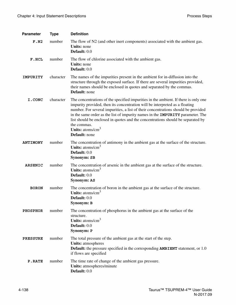
Chapter 4: Input Statement Descriptions Process Steps

F.N2 number The flow of N2 (and other inert components) associated with the ambient gas. Units: none Default: 0.0

F.HCL number The flow of chlorine associated with the ambient gas. Units: none Default: 0.0

IMPURITY character The names of the impurities present in the ambient for in-diffusion into the structure through the exposed surface. If there are several impurities provided, their names should be enclosed in quotes and separated by the commas.Default: none

I.CONC character The concentrations of the specified impurities in the ambient. If there is only one impurity provided, then its concentration will be interpreted as a floating number. For several impurities, a list of their concentrations should be provided in the same order as the list of impurity names in the IMPURITY parameter. The list should be enclosed in quotes and the concentrations should be separated by the commas.Units: atoms/cm3

Default: none

ANTIMONY number The concentration of antimony in the ambient gas at the surface of the structure. Units: atoms/cm3 Default: 0.0 Synonym: SB

ARSENIC number The concentration of arsenic in the ambient gas at the surface of the structure. Units: atoms/cm3 Default: 0.0 Synonym: AS

BORON number The concentration of boron in the ambient gas at the surface of the structure. Units: atoms/cm3 Default: 0.0 Synonym: B

PHOSPHOR number The concentration of phosphorus in the ambient gas at the surface of the structure. Units: atoms/cm3 Default: 0.0 Synonym: P

PRESSURE number The total pressure of the ambient gas at the start of the step. Units: atmospheres Default: the pressure specified in the corresponding AMBIENT statement, or 1.0 if flows are specified

P.RATE number The time rate of change of the ambient gas pressure. Units: atmospheres/minute Default: 0.0

Parameter Type Definition

4-138 Taurus™ TSUPREM-4™ User GuideN-2017.09

Process Steps Chapter 4: Input Statement Descriptions

Description This statement specifies a diffusion step, with or without oxidation. Any impurities present in the wafer are diffused. If the wafer is exposed to a gas, predeposition and/or oxidation can be performed. If an oxidizing ambient is specified and the VISCOUS oxidation model is in effect, reflow of surface layers occurs.

The duration of the step must be specified with the TIME parameter. The ambient temperature must be specified with the TEMPERAT keyword (unless CONTINUE is specified). For linear ramping of the temperature, specify either the ramp rate (with T.RATE) or the temperature at the end of the step (with T.FINAL).

Ambient Gas The ambient gas used during the diffusion step can be specified in one of two ways:

• Specify one of the DRYO2, WETO2, STEAM, INERT, or AMB.1 through AMB.5 parameters. These select an ambient that has been predefined with the AMBIENT statement. The DRYO2, WETO2, STEAM, and INERT ambients are defined by the standard initialization file; the AMB.1 through AMB.5 ambients must be defined by the user before they are used. The predefined ambients include a default pressure and HCl percentage, which can be overridden with the PRESSURE and HCL parameters, respectively, on the DIFFUSION statement.

• Define the ambient by specifying the flows of oxidizing (O2 and H2O) and nonoxidizing (H2, N2, and HCl) species. The flows can be specified as flow

P.FINAL number The ambient gas pressure at the end of the step. Units: atmospheres Default: PRESSURE

HCL number The percentage of chlorine present in the ambient gas. Units: percent Default: value calculated from F.HCL or specified on AMBIENT statement

D.RECOMB number The fraction of Frenkel pair implant damage remaining after initial recombination.Units: noneDefault: 0.0

MOVIE character A string of TSUPREM-4 commands to be executed at the beginning of each time step. Multiple input statements can be given, separated by semicolons (;). Default: no commands executed

DUMP number Write a solution file after every DUMP time step. The files are readable with the LOADFILE and INITIALIZE statements. The names are of the form steam>, where <time> is the time in seconds from the start of the diffusion step. Units: none Default: no intermediate solutions saved

Parameter Type Definition

Taurus™ TSUPREM-4™ User Guide 4-139N-2017.09

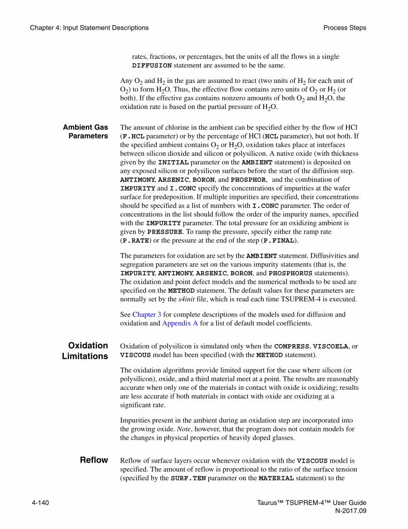
Chapter 4: Input Statement Descriptions Process Steps

rates, fractions, or percentages, but the units of all the flows in a single DIFFUSION statement are assumed to be the same.

Any O2 and H2 in the gas are assumed to react (two units of H2 for each unit of O2) to form H2O. Thus, the effective flow contains zero units of O2 or H2 (or both). If the effective gas contains nonzero amounts of both O2 and H2O, the oxidation rate is based on the partial pressure of H2O.

Ambient GasParameters

The amount of chlorine in the ambient can be specified either by the flow of HCl (F.HCL parameter) or by the percentage of HCl (HCL parameter), but not both. If the specified ambient contains O2 or H2O, oxidation takes place at interfaces between silicon dioxide and silicon or polysilicon. A native oxide (with thickness given by the INITIAL parameter on the AMBIENT statement) is deposited on any exposed silicon or polysilicon surfaces before the start of the diffusion step. ANTIMONY, ARSENIC, BORON, and PHOSPHOR, and the combination of IMPURITY and I.CONC specify the concentrations of impurities at the wafer surface for predeposition. If multiple impurities are specified, their concentrations should be specified as a list of numbers with I.CONC parameter. The order of concentrations in the list should follow the order of the impurity names, specified with the IMPURITY parameter. The total pressure for an oxidizing ambient is given by PRESSURE. To ramp the pressure, specify either the ramp rate (P.RATE) or the pressure at the end of the step (P.FINAL).

The parameters for oxidation are set by the AMBIENT statement. Diffusivities and segregation parameters are set on the various impurity statements (that is, the IMPURITY, ANTIMONY, ARSENIC, BORON, and PHOSPHORUS statements). The oxidation and point defect models and the numerical methods to be used are specified on the METHOD statement. The default values for these parameters are normally set by the s4init file, which is read each time TSUPREM-4 is executed.

See Chapter 3 for complete descriptions of the models used for diffusion and oxidation and Appendix A for a list of default model coefficients.

OxidationLimitations

Oxidation of polysilicon is simulated only when the COMPRESS, VISCOELA, or VISCOUS model has been specified (with the METHOD statement).

The oxidation algorithms provide limited support for the case where silicon (or polysilicon), oxide, and a third material meet at a point. The results are reasonably accurate when only one of the materials in contact with oxide is oxidizing; results are less accurate if both materials in contact with oxide are oxidizing at a significant rate.

Impurities present in the ambient during an oxidation step are incorporated into the growing oxide. Note, however, that the program does not contain models for the changes in physical properties of heavily doped glasses.

Reflow Reflow of surface layers occur whenever oxidation with the VISCOUS model is specified. The amount of reflow is proportional to the ratio of the surface tension (specified by the SURF.TEN parameter on the MATERIAL statement) to the

4-140 Taurus™ TSUPREM-4™ User GuideN-2017.09

Process Steps Chapter 4: Input Statement Descriptions

viscosity for each material. Reflow can occur in any material having a nonzero value of SURF.TEN. Only exposed layers flow due to surface tension, but underlying layers can deform due to stresses produced by reflow of the exposed layers.

Reflow in an inert ambient can be approximated by specifying an oxidizing ambient with a negligible partial pressure of oxidant (for example, by setting PRESSURE=1e-6 or by a combination such as F.N2=1.0 and F.O2=1e-6). Note that a native oxide is added whenever the partial pressure of the oxidizing species is nonzero; it may be necessary to do a shallow etch to remove this oxide following a reflow step.

Examples 1. The following statement specifies a 1000-deg, 30-min boron predeposition:

DIFFUSION TIME=30 TEMP=1000 BORON=1E20

2. The following statement calls for a 30-min diffusion in an inert ambient:

DIFFUSION TIME=30 TEMP=800 T.FINAL=1000 INERT

The temperature is ramped from 800° to 1000°C during the step.

3. The following statement calls for a 60-min dry oxidation at 900°C with an ambient containing 2% HCl:

DIFFUSION TIME=60 TEMP=900 DRYO2 HCL=2

4. The following statement performs a 30-min, 1000°C diffusion:

DIFFUSION TIME=30 TEMP=1000 + MOVIE="SELECT Z=log10(Boron)

PLOT.1D X.V=1.0"

The boron concentration is plotted before each time step.

Taurus™ TSUPREM-4™ User Guide 4-141N-2017.09

Chapter 4: Input Statement Descriptions Process Steps

EPITAXY

The EPITAXY statement is used to grow silicon material on the exposed silicon surface of the current structure.

EPITAXY TIME=<n> TEMPERAT=<n> [ {T.RATE=<n> | T.FINAL=<n>} ] [IMPURITY=<c>

{ IT.CONC=<c> [IB.CONC=<c>] [LOG.GRAD] | I.PROFIL=<c> | I.RESIST=<n> } ]

[ANTIMONY=<n>] [ARSENIC=<n>] [BORON=<n>] [PHOSPHOR=<n>] [ {CONCENTR | RESISTIV} ] THICKNES=<n> [SPACES=<n>] [DY=<n>] [YDY=<n>] [ARC.SPAC=<n>]

[AR.MIN=<n>] [SELECTIV] [MOVIE=<c>] [BLANKET][DIFFUSED][STRAINED][CONTINUE]

Parameter Type Definition

TIME number The duration of the epitaxy step. Units: minutes Default: none

TEMPERAT number The ambient temperature at the beginning of the step. Units: °Celsius Default: none

T.RATE number The time rate of change of the ambient temperature. Units: °Celsius/minute Default: 0.0

T.FINAL number The ambient temperature at the end of the step. Units: °Celsius Default: TEMPERAT

IMPURITY character The names of the impurities with which the epitaxial layer is doped. If there are several impurities provided, their names should be enclosed in quotes and separated by the commas.Default: none

IT.CONC character The concentrations of the specified impurities in the epitaxial layer. If there is only one impurity provided, then its concentration will be interpreted as a floating number. For several impurities, a list of their concentrations should be provided in the same order as the list of impurity names in the IMPURITY parameter. The list should be enclosed in quotes and the concentrations should be separated by the commas.Units: atoms/cm3

Default: none

4-142 Taurus™ TSUPREM-4™ User GuideN-2017.09

Process Steps Chapter 4: Input Statement Descriptions

IB.CONC character The impurity concentrations at the bottom of the grown layer of the impurity species listed in the IMPURITY parameter. The impurity concentrations at the top of the layer must be specified by the IT.CONC parameter.Units: atoms/cm3

Default: uniform impurity concentrations specified by IT.CONC

LOG.GRAD logical Specifies that the impurity concentrations specified by IMPURITY will vary logarithmically between the values specified by IB.CONC and IT.CONC.Default: false

I.PROFIL character The expression string for an equation that specifies the concentration of the single impurity specified by IMPURITY as a function of F, the fraction of the total layer thickness (or epitaxy time). F must obey the rules for a DEFINE variable; it is recommended that it always by enclosed in braces and preceded by the "@" character; that is, it should always appear as "@{F}" in the equation.Units: atoms/cm3

Default: none

I.RESIST number The resistivity produced by the presence of IMPURITY in the ambient gas at the surface of the wafer.Units: ohm-cmDefault: none

ANTIMONY number The uniform concentration or resistivity of antimony in the deposited layer. Units: atoms/cm3 or ohm-cm Default: zero concentration Synonym: SB

ARSENIC number The uniform concentration or resistivity of arsenic in the deposited layer. Units: atoms/cm3 or ohm-cm Default: zero concentration Synonym: AS

BORON number The uniform concentration or resistivity of boron in the deposited layer. Units: atoms/cm3 Default: zero concentration Synonym: B

PHOSPHOR number The uniform concentration or resistivity of phosphorus in the deposited layer. Units: atoms/cm3 or ohm-cm Default: zero concentration Synonym: P

CONCENTR logical Specifies that the impurity concentration in the deposited layer is given. Default: true

RESISTIV logical Specifies that the resistivity of the deposited layer is given. Default: false

THICKNES number The thickness of the deposited layer. Units: microns Default: none

Parameter Type Definition

Taurus™ TSUPREM-4™ User Guide 4-143N-2017.09

Chapter 4: Input Statement Descriptions Process Steps

SPACES number The number of vertical grid spacings in the layer. This value is divided by the value of GRID.FAC (see MESH, p. 4-52).Units: noneDefault: 1/GRID.FAC Synonym: DIVISION

DY number The nominal grid spacing to be used in the deposited material layer at the location specified by the YDY parameter. This value is multiplied by the value of GRID.FAC (see MESH, p. 4-52).Units: microns Default: GRID.FAC*THICKNES/SPACES Synonym: DX

YDY number The location of the nominal grid spacing specified by DY, relative to the top of the deposited layer. Units: microns)Default: 0.0Synonym: XDX

ARC.SPAC number The maximum spacing allowed along an arc on the new surface. This value is multiplied by the value of GRID.FAC (see MESH, p. 4-52).Units: micronsDefault: 0.5*THICKNES*GRID.FAC

AR.MIN number The minimum aspect (width/height) ratio for deposited grid spaces on planar surfaces.Default: 0.5

SELECTIV logical Specifies that material will only be grown on silicon or polysilicon surfaces. Default: false

MOVIE character A string of TSUPREM-4 commands to be executed at the beginning of each time step. Multiple input statements can be given, separated by semicolons (;). Default: no commands executed

BLANKET logical Specifies that grown material will be single-crystal silicon, regardless of the underlying material. Default: false

DIFFUSED logical Specifies to solve the diffusion equations.Default: true

STRAINED logical Specifies to add lattice mismatch strains to epitaxial layers. Only applicable with the VISCOEL and ST.HIST models.Default: false

CONTINUE logical Specifies to continue the time step instead of starting with INIT.TIM for each incremental epitaxial deposition. Turning on CONTINUE reduces the simulation time, especially when more grid spaces are allocated in the epitaxial layer.Default: false

Parameter Type Definition

4-144 Taurus™ TSUPREM-4™ User GuideN-2017.09

Process Steps Chapter 4: Input Statement Descriptions

Description This statement provides a basic epitaxy capability. Silicon is deposited on the exposed surface of the structure, and its upper surface becomes the new exposed surface. A uniform concentration of each dopant can be specified, either directly or by the resistivity of the grown material. Impurities diffuse according to the models in Chapter 3, Diffusion, p. 3-14.

By default, (single-crystal) silicon is grown on (single-crystal) silicon surfaces, and polysilicon is grown on all other surface materials. If SELECTIV is set true, growth occurs only on silicon and polysilicon surfaces and no growth occurs on other materials. If BLANKET is set true, then all grown material will be single-crystal silicon, regardless of the underlying material. Setting BLANKET true and leaving SELECTIV false causes a uniform layer of single-crystal silicon to be grown over the entire surface, as in older versions of the program.

The deposited material conforms to the contours of the original surface. Outside corners on the original surface produce arcs on the new surface, which are approximated by straight line segments. The maximum segment length is set by the ARC.SPAC parameter.

The SPACES, DY, and YDY parameters used to control the grid spacing in the deposited layer are scaled by the value of the GRID.FAC parameter on the MESH statement (see Chapter 3, Changes to the Mesh During Processing, p. 3-7).

The EPITAXY statement works by alternately depositing layers and diffusing impurities in the resulting structure. The number of deposit/diffuse steps is equal to the number of grid spaces in the deposited layer (that is, it is controlled by the SPACES, DY, and YDY parameters). The horizontal spacing in a thin deposited layer is the same as in the substrate, but for thick layers it is increased to avoid mesh elements with high ratios of height to width. This increase in horizontal spacing can be controlled with the AR.MIN parameter.

If multiple impurities are specified, their concentrations should be specified as a list of numbers with I.CONC parameter. The order of concentrations in the list should follow the order of the impurity names, specified with the IMPURITY parameter

Gradient-DopedGrowth

If IB.CONC is specified, the impurities named in the IMPURITY parameter will have the concentrations IB.CONC at the bottom of the deposited or grown layer and the concentrations IT.CONC at the top of the layer. The concentration will vary linearly through the layer, unless LOG.GRAD is specified; in this case, the variation will be logarithmic. IB.CONC can only be used when IMPURITY and IT.CONC (alias I.CONC) are also specified.

If I.PROFIL is specified, it is interpreted as an equation specifying the concentration of a single impurity (specified by IMPURITY) as a function of F, the fraction of the layer thickness (F=0 at the bottom of the layer and F=1 at the top). The parameter F must obey the rules for a DEFINE variable; it is recommended that it be enclosed in braces and preceded by the "@" character, that is, "@{F}".

Taurus™ TSUPREM-4™ User Guide 4-145N-2017.09

Chapter 4: Input Statement Descriptions Process Steps

Note: The doping at interior nodes in the deposited layer is calculated by linear or logarithmic interpolation or by I.PROFIL. Thus, the total dose will be expected to differ from that calculated by analytical integration of the specified gradient (except in the special case of a linear gradient and a uniformly spaced grid).

Example 1. The following statement deposits 1 micron of silicon while simultaneously diffusing at 1100°C:

EPITAXY THICK=1.0 TIME=180 TEMPERAT=1100 +ANTIMONY=1E19 SPACES=10

The deposition and diffusion processes are subdivided into 10 steps corresponding to the value specified by the SPACES parameter.

2. Epitaxial growth with linear gradient boron profile:

EPITAXY TIME=10 TEMP=600 THICK=0.1 IMP=BORON +IB.CONC=1E14 IT.CONC=1E15 SPACES=20

3. Same as 2. But use I.PROFILE:

EPITAXY TIME=10 TEMP=600 THICK=0.1 IMP=BORON +I.PROFIL=( 5E12*(5E13/5E12)^@{F} ) SPACES=20

4. Epitaxial growth with logarithmic gradient boron profile:

EPITAXY TIME=10 TEMP=600 THICK=0.1 IMP=BORON +IB.CONC=1E14 IT.CONC=1E15 SPACES=20 LOG.GRAD

5. Epitaxy with logarithmic gradient multiple species:

EPITAXY THICK=0.2 SPACES=10 TIME=10 TEMP=600 +IMP="BORON, PHOSPHORUS" +IB.CONC="5E13 5E15" +I.CONC="5E14 2E15" LOG.GRAD

Note:The mobility tables used to calculate the doping from the resistive are not the same as the tables used by the ELECTRICAL statement. The extracted sheet resistance for the epitaxial layer does not correspond exactly to the resistivity specified during epitaxy.

4-146 Taurus™ TSUPREM-4™ User GuideN-2017.09

Process Steps Chapter 4: Input Statement Descriptions

STRESS

The STRESS statement solves the stress equation only to calculate the stresses caused by thermal mismatch between materials, imbalanced forces, or due to external pressure for applications in chip packaging.

STRESS

{ ( TIME=<n> TEMPERAT=<n> [ {T.RATE=<n> | T.FINAL=<n>} ][MOVIE=<c>])

| ( [ P.TOP=<n>] [P.SIDE=<n>] )| RELAX

}

Parameter Type Definition

TIME number The duration of the stress step. Units: minutesDefault: none

TEMPERAT number The ambient temperature at the beginning of the step. Units: °Celsius Default: none

T.RATE number The time rate of change of the ambient temperature. Units: °Celsius/minute Default: 0.0

T.FINAL number The ambient temperature at the end of the step. Units: °Celsius Default: TEMPERAT+T.RATE×TIME

MOVIE character A string of TSUPREM-4 commands to be executed at the beginning of each time step. Multiple input statements can be given, separated by semicolons (;). Default: no commands executed

P.TOP number The applied pressure on the top exposed surface. Units: dynes/cm^2Default: 0.0

P.SIDE number The applied pressure on the right side surface. Units: dynes/cm^2Default: 0.0

RELAX logical Specifies to perform the stress relaxationDefault: false

Taurus™ TSUPREM-4™ User Guide 4-147N-2017.09

Chapter 4: Input Statement Descriptions Process Steps

Description This statement calculates stresses due to thermal mismatch between materials, imbalanced forces, or external pressure for chip packaging applications. The STRESS command is applicable only when the Boolean parameters ST.HIST and VISCOEL are switched on in the METHOD statement.

Thermal Mismatch For thermal mismatch stresses, only stress equations are solved for the specified temperature change. Parameter TEMPERATURE specifies the initial temperature. TIME specifies the duration time of the step, T.RATE specifies the temperature change rate, and T.FINAL specifies the final temperature of the ramp. If the duration time is zero, or the temperature change rate is zero, or the final temperature is equal to the initial temperature. STRESS command updates only the stress values by solving the stress equations while the values of the other solutions are kept. Thus, the temperature at which stress values are calculated, hereinafter stress temperature must be distinguished from the diffusion temperature. During all thermal processes but the STRESS command, the stress temperature is always identical to the diffusion temperature. Both the diffusion temperature and the stress temperature are saved to an output file.

DIFFUSION TEMP=@DTEMP1 TIME=1 ;$(1)STRESS TEMP=@STEMP1 T.FINAL=@STEMP2 TIME=1 ;$(2)DIFFUSION TEMP=@DTEMP2 TIME=1 ;$(3)

• At (1), the diffusion equations and the stress equations are solved at DTEMP1. (stress temperature = diffusion temperature = DTEMP1).

• At (2), when STEMP1 is different from DTEMP1, the stress equations are solved first for the temperature ramp from DTEMP1 to STEMP1 before processing from STEMP1 to STEMP2. The final stress temperature is STEMP2 while the diffusion temperature keeps DTEMP1, which means all equilibrium values associated with diffusion are calculated at DTEMP, while the stress are calculated at STEMP2 (stress temperature = STEMP2, diffusion temperature = DTEMP1).

• At (3), When STEMP2 is different from DTEMP1, the stress equations are solved first for the temperature ramp from STEMP2 to DTEMP1 before processing the diffusion step. Then, in processing the diffusion step, when DTEMP2 is different from DTEMP1, the diffusion equations and the stress equations are solved for the temperature ramp from DTEMP1 to DTEMP2 before processing 1-minute diffusion at DTEMP2. (stress temperature = diffusion temperature = DTEMP2).

• The time step for the internal temperature ramp is specified by the TIME.DEL parameter in the METHOD statement.

• If TEMPERAT is not specified, the latest stress temperature is used for initial temperature.

Relaxation Simply specifying the RELAX parameter forces the instantaneous stress relaxation:

STRESS RELAX

4-148 Taurus™ TSUPREM-4™ User GuideN-2017.09

Process Steps Chapter 4: Input Statement Descriptions

External Pressure For stresses due to pressure boundary condition, P.TOP specifies the value of the applied pressure on the top exposed surface, and P.SIDE specifies the value of the applied pressure on the right side surface. To apply the pressure boundary condition, the original reflective boundary condition is removed. This feature is intended for chip packaging application only and the drastic change of boundary condition can lead to multiple complications depending on the applications.

Printing andPlotting of

Stresses andDisplacements

The calculated stresses can be accessed for printing or plotting by referencing the variables Sxx, Syy, and Sxy on the SELECT statement; the calculated x and y displacements can be referenced as x.vel and y.vel. The stresses and displacements can also be displayed with the STRESS and FLOW parameters on the PLOT.2D statement.

Example The following statement calculates the thermal mismatch stress between materials due to a temperature ramp from 50° to 1050°C with duration time of 1 minute:

STRESS TIME=1 TEMPERATURE=50 T.FINAL=1050

The Following statement calculates the stresses due to packaging pressure of 500e6 dynes/cm2 applied on the top surface:

STRESS P.TOP=500e6

Taurus™ TSUPREM-4™ User Guide 4-149N-2017.09

Chapter 4: Input Statement Descriptions Output

OutputThe following statements print and plot results:

Statement Name Description Page

SELECT Evaluates the quantity to be printed or plotted; specifies titles and axis labels.

p. 4-151

PRINT.1D Prints values of a quantity along a line through the structure.

p. 4-156

PLOT.1D Plots a quantity along a line through the structure. p. 4-160

PLOT.2D Plots axes and boundaries for 2D structure plots; plots grid and/or velocity and stress vectors.

p. 4-168

CONTOUR Plots contours in two dimensions. p. 4-173

COLOR Fills areas of a 2D plot. p. 4-175

PLOT.3D Plots a 3D projection plot of the selected quantity. p. 4-177

LABEL Adds labels to a plot. p. 4-180

EXTRACT Extracts information about a structure, and prints it or writes it to a file.

p. 4-185

ELECTRICAL Extracts electrical information, and prints it or writes it to a file.

p. 4-198

VIEWPORT Specifies a subset of the plotting surface to plot on. p. 4-207

4-150 Taurus™ TSUPREM-4™ User GuideN-2017.09

Output Chapter 4: Input Statement Descriptions

SELECT

The SELECT statement evaluates a quantity to be printed or plotted. It is also used to specify plot titles and axis labels.

Description The SELECT statement evaluates the quantity to be displayed by the CONTOUR, PLOT.1D, PRINT.1D, PLOT.2D, and PLOT.3D statements or to be extracted by the EXTRACT statement. No solution data can be printed or plotted until this statement is specified. The values calculated by a SELECT statement are used until another SELECT statement is specified. If the solution changes, a new SELECT statement is given in order for the new values to be printed or plotted.

Solution Values The Z parameter specifies a mathematical expression for the quantity to be plotted. The following solution values can be used in the expression, provided that the solution is available:

SELECT [Z=<c>] [TEMPERAT=<n>] [LABEL=<c>] [TITLE=<c>]

Parameter Type Definition

Z character A mathematical expression defining the quantity to be printed or plotted. If the expression contains spaces, it must be enclosed in parentheses. Default: “0”

TEMPERAT number The temperature at which the solution is to be evaluated.Units: degrees Celsius Default: last specified temperature or 800

LABEL character The label to be used on the y axis of a 1D plot, or the z axis of a three-dimensional plot.Default: the expression given by Z

TITLE character The title to be used on plots. Default: the name and version number of the program

antimony antimony concentration (atoms/cm3)

arsenic arsenic concentration (atoms/cm3)

boron boron concentration (atoms/cm3)

phosphorus phosphorus concentration (atoms/cm3)

indium indium concentration (atoms/cm3)

i_antimony antimony interface trap density (atoms/cm2)

i_arsenic arsenic interface trap density (atoms/cm2)

i_boron boron interface trap density (atoms/cm2)

Taurus™ TSUPREM-4™ User Guide 4-151N-2017.09

Chapter 4: Input Statement Descriptions Output

i_phosphorus phosphorus interface trap density (atoms/cm2)

c0_antimony antimony precipitation concentration (atoms/cm3)

c0_arsenic arsenic precipitation concentration (atoms/cm3)

c0_boron boron precipitation concentration (atoms/cm3)

c0_phosphor phosphorus precipitation concentration (atoms/cm3)

c1_antimony antimony-interstitial cluster concentration (atoms/cm3)

c1_arsenic arsenic-interstitial cluster concentration (atoms/cm3)

c1_boron boron-interstitial cluster concentration (atoms/cm3)

c1_phosphor phosphorus-interstitial cluster concentration (atoms/cm3)

c2_antimony antimony-vacancy cluster concentration (atoms/cm3)

c2_arsenic arsenic-vacancy cluster concentration (atoms/cm3)

c2_boron boron-vacancy cluster concentration (atoms/cm3)

c2_phosphor phosphorus-vacancy cluster concentration (atoms/cm3)

ipair_antimony antimony-interstitial pair concentration (atoms/cm3)

ipair_arsenic arsenic-interstitial pair concentration (atoms/cm3)

ipair_boron boron-interstitial pair concentration (atoms/cm3)

ipair_phosphor phosphorus-interstitial concentration (atoms/cm3)

vpair_antimony antimony-vacancy pair concentration (atoms/cm3)

vpair_arsenic arsenic-vacancy pair concentration (atoms/cm3)

vpair_boron boron-vacancy pair concentration (atoms/cm3)

vpair_phosphor phosphorus-vacancy concentration (atoms/cm3)

doping net active concentration (atoms/cm3)

oxygen oxidant concentration (atoms/cm3)

silicon silicon concentration (in silicide) (atoms/cm3)

interstitial interstitial concentration (#/cm3)

vacancy vacancy concentration (#/cm3)

damage damage concentration (#/cm3)

ci.star equilibrium interstitial concentration (#/cm3)

cv.star equilibrium vacancy concentration (#/cm3)

trap concentration of filled interstitial traps (#/cm3)

cl_interst concentration of clustered interstitials (#/cm3)

cl_im0 concentration of interstitial clusters (#/cm3)

dloop density of dislocation loops (#/cm3)

rloop radius of dislocation loops (cm)

4-152 Taurus™ TSUPREM-4™ User GuideN-2017.09

Output Chapter 4: Input Statement Descriptions

The names of user-specified impurities can also be used, giving the concentration of the impurity in atoms/cm3.

• The chemical concentration is reported unless the active function is used, for example, active(phosphorus).

• The net concentration is defined as the sum of the donor concentrations minus the sum of the acceptor concentrations.

• The electron concentration is calculated using the assumptions of local charge neutrality and complete ionization of impurities.

• The dopant-interstitial and dopant-vacancy pair concentration in local equilibrium are calculated by, for example, eqipair(boron) and eqvpair(boron) for boron.

• Any intermediates.

MathematicalOperations and

Functions

The symbols “+”, “-”, “*”, “/”, and “^” are used for the mathematical operations of addition, subtraction, multiplication, division, and exponentiation, respectively. In addition, the following functions are available:

lgrain average polycrystalline grain size (um)

electron concentration of electrons (#/cm3)

x.v x velocity (cm/s)

y.v y velocity (cm/s)

Sxx, Sxy, Syy components of the stress tensor (dynes/cm2)

x x coordinate (microns)

y y coordinate (microns)

abs absolute value

active electrically active part of impurity concentration

asin, acos, atan

inverse trigonometric functions (results in radians)

diffusivity diffusivity (in cm2/s) of an impurity or point defect species

eqactive electrically active part of impurity concentration in equilibrium

eqipair dopant-interstitial pair concentration of an impurity in local equilibrium

eqvpair dopant-vacancy pair concentration of an impurity in local equilibrium

erf error function

erfc complementary error function

exp exponential

gb concentration of impurity in polycrystalline grain boundaries

Taurus™ TSUPREM-4™ User Guide 4-153N-2017.09

Chapter 4: Input Statement Descriptions Output

The log, log10, and slog10 functions return the value 0.0 if their argument is zero; the log, log10, slog10, and sqrt functions take absolute value of their arguments. The following constant is available:

Note:The active and net concentrations depend on the temperature. If TEMPERAT is not specified, the last processing temperature is used. If the last process step ended with a ramp to a low temperature, you may need to specify a higher value of TEMPERAT to obtain realistic levels of dopant activation.

Examples 1. The logarithm (base 10) of the arsenic concentration is evaluated with:

SELECT Z=log10(Arsenic)

2. The phosphorus concentration minus a constant profile of 5x1014 is evaluated with:

SELECT Z=(Phosphorus - 5.0e14)

3. The difference between the phosphorus concentration and an analytic profile is evaluated with:

SELECT Z=(phos - 1.0e18 * exp ( y * y ) )

4. The excess vacancy-interstitial product is evaluated with:

SELECT Z=(inter * vacan - ci.star * cv.star)

5. The diffusivity (in cm2/s) of boron at each point in the structure is evaluated with:

SELECT Z=diffusivity(Boron)

log natural logarithm of the absolute value

log10 base-10 logarithm of the absolute value

sinh, asinh, cosh, acosh, tanh, atanh

hyperbolic and inverse hyperbolic functions

slog10 base-10 logarithm of the absolute value times the sign of the value

sqrt square root

sin, cos, tan trigonometric functions (arguments in radians)

rand random number function (the argument is a seed)returns the random number between 0.0 and 1.0

Kb Boltzmann’s constant (eV/°C)

4-154 Taurus™ TSUPREM-4™ User GuideN-2017.09

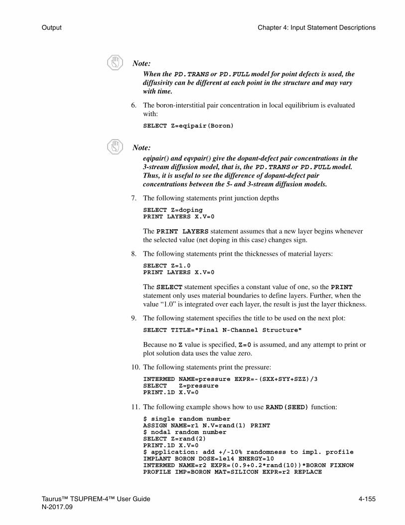
Output Chapter 4: Input Statement Descriptions

Note:When the PD.TRANS or PD.FULL model for point defects is used, the diffusivity can be different at each point in the structure and may vary with time.

6. The boron-interstitial pair concentration in local equilibrium is evaluated with:

SELECT Z=eqipair(Boron)

Note:eqipair() and eqvpair() give the dopant-defect pair concentrations in the 3-stream diffusion model, that is, the PD.TRANS or PD.FULL model. Thus, it is useful to see the difference of dopant-defect pair concentrations between the 5- and 3-stream diffusion models.

7. The following statements print junction depths

SELECT Z=dopingPRINT LAYERS X.V=0

The PRINT LAYERS statement assumes that a new layer begins whenever the selected value (net doping in this case) changes sign.

8. The following statements print the thicknesses of material layers:

SELECT Z=1.0PRINT LAYERS X.V=0

The SELECT statement specifies a constant value of one, so the PRINT statement only uses material boundaries to define layers. Further, when the value “1.0” is integrated over each layer, the result is just the layer thickness.

9. The following statement specifies the title to be used on the next plot:

SELECT TITLE="Final N-Channel Structure"

Because no Z value is specified, Z=0 is assumed, and any attempt to print or plot solution data uses the value zero.

10. The following statements print the pressure:

INTERMED NAME=pressure EXPR=-(SXX+SYY+SZZ)/3SELECT Z=pressurePRINT.1D X.V=0

11. The following example shows how to use RAND(SEED) function:

$ single random numberASSIGN NAME=r1 N.V=rand(1) PRINT$ nodal random numberSELECT Z=rand(2)PRINT.1D X.V=0$ application: add +/-10% randomness to impl. profileIMPLANT BORON DOSE=1e14 ENERGY=10INTERMED NAME=r2 EXPR=(0.9+0.2*rand(10))*BORON FIXNOWPROFILE IMP=BORON MAT=SILICON EXPR=r2 REPLACE

Taurus™ TSUPREM-4™ User Guide 4-155N-2017.09

Chapter 4: Input Statement Descriptions Output

PRINT.1D

The PRINT.1D statement prints the value of the selected expression along a line through the structure. It can also print layer thickness and integrated doping information.

PRINT.1D { X.VALUE=<n> | Y.VALUE=<n> | ( { MATERIAL=<c> | SILICON | OXIDE | OXYNITRI | NITRIDE | POLYSILI | PHOTORES | ALUMINUM } { /MATERIA=<c> | /SILICON | /OXIDE | /OXYNITR | /NITRIDE | /POLYSIL | /PHOTORE | /ALUMINU | /AMBIENT | /REFLECT } ) } [OUT.FILE=<c> [APPEND] [{CM | UM | NM}] [SPOT=<n>] [LAYERS] [X.MIN=<n>] [X.MAX=<n>]

Parameter Type Definition

X.VALUE number The x coordinate of a vertical section along which values are to be printed. Units: microns Default: 0.0

Y.VALUE number The y coordinate of a horizontal section along which values are to be printed. Units: microns Default: none

MATERIAL character Print values in the named material, at the interface with the other specified material.Default: none

SILICON logical Print values in silicon, at the interface with the other specified material. Default: false

OXIDE logical Print values in oxide, at the interface with the other specified material. Default: false

OXYNITRI logical Print values in oxynitride, at the interface with the other specified material.Default: false

NITRIDE logical Print values in nitride, at the interface with the other specified material. Default: false

POLYSILI logical Print values in polysilicon, at the interface with the other specified material. Default: false

PHOTORES logical Print values in photoresist, at the interface with the other specified material. Default: false

4-156 Taurus™ TSUPREM-4™ User GuideN-2017.09

Output Chapter 4: Input Statement Descriptions

ALUMINUM logical Print values in aluminum, at the interface with the other specified material. Default: false

/MATERIA character Print values in the other specified material, at the interface with the named material.Default: none

/SILICON logical Print values in the other specified material, at the interface with silicon. Default: false

/OXIDE logical Print values in the other specified material, at the interface with oxide. Default: false

/OXYNITR logical Print values in the other specified material, at the interface with oxynitride. Default: false

/NITRIDE logical Print values in the other specified material, at the interface with nitride. Default: false

/POLYSIL logical Print values in the other specified material, at the interface with polysilicon. Default: false

/PHOTORE logical Print values in the other specified material, at the interface with photoresist. Default: false

/ALUMINU logical Print values in the other specified material, at the interface with aluminum. Default: false

/AMBIENT logical Print values in the other specified material, at the interface with the exposed surface (if any). Default: false Synonym: /EXPOSED, /GAS

/REFLECT logical Print values in the other specified material, at the interface with the reflecting boundary (if any). Default: false

OUT.FILE character The name of the output file in which the printed profile is saved.Default: data not written to file

APPEND logical Specifies that saved profiles are to be appended to the file specified by OUT.FILE. If APPEND is false, any existing data in the specified file are discarded before writing the new data.Default: false

CM logical Specifies that the distances are to be printed in centimeters.Default: false

UM logical Specifies that the distances are to be printed in microns.Default: true

NM logical Specifies that the distances are to be printed in nanometers.Default: false

Parameter Type Definition

Taurus™ TSUPREM-4™ User Guide 4-157N-2017.09

Chapter 4: Input Statement Descriptions Output

Description The PRINT.1D statement prints the values of the selected quantity along a cross-section through the device. Cross-sections are defined as vertical or horizontal (by the X.VALUE and Y.VALUE parameters, respectively), along the interface between two materials, or along a boundary of the device structure. The quantity to be printed must be specified on a SELECT statement preceding the PRINT.1D statement. The SPOT parameter finds all points along the specified path at which the selected quantity equals the specified value.

Layers If LAYERS is specified, the integral of the selected quantity over each layer is printed. The integration is along the path defined by the X.VALUE, Y.VALUE, or interface specification. Layers are delimited by those points along the path where the material type changes or the sign of the selected quantity changes. If a cross-section passes out a structure into the ambient and then re-enters the structure, the ambient “layer” may be omitted from the LAYERS output.

Interface Values The values along the interface between two materials depend on the order in which the materials are specified. Thus SILICON /OXIDE and OXIDE /SILICON print values at the same interface, but the first prints the values in the silicon, while the second prints the values in the oxide.

Values along an interface are sorted by their x coordinates. The values printed may not be in order if there are vertical or re-entrant interfaces, or if the structure contains more than one interface between the specified materials.

Saving Profiles ina File

If OUT.FILE is specified, profiles printed by PRINT.1D are saved in a file. The file contains the same information that is sent to the standard output except that a ‘/’ is substituted for the first blank space in the heading line. Thus the file consists of a heading line (with a ‘/’ in the first column) followed by a series of data lines, each containing three values: the x or y location, the solution value (specified by

SPOT number Print the coordinate along the cross-section at which the selected quantity equals the specified value. Units: units of the selected quantity Default: none

LAYERS logical Report the integral of the selected quantity over each layer of the device structure. Default: false

X.MIN number The minimum position along the cross-section to be printed. Units: microns Default: none

X.MAX number The maximum position along the cross-section to be printed. Units: microns Default: none

Parameter Type Definition

4-158 Taurus™ TSUPREM-4™ User GuideN-2017.09

Output Chapter 4: Input Statement Descriptions

the Z parameter on a preceding SELECT statement), and the material type. Results produced by the SPOT and LAYERS parameters are not saved in the file. If APPEND is specified, the profile information is appended following any previously existing data in the output file; if APPEND is false (the default), existing data in the output file is discarded before the new information is saved. Files produced by the OUT.FILE parameter on the PRINT.1D statement can be read with the PROFILE statement or used as targets for optimizing profiles.

Examples 1. The following statements print the boron concentration at x=1.0 micron between the top of the mesh and y=3.0 microns:

SELECT Z=BoronPRINT.1D X.VAL=1.0 X.MAX=3.0 OUT.FILE=boron.dat

The profile is saved in the file boron.dat.

2. The following statements print the x and y coordinates of the interface between silicon and oxide:

SELECT Z=yPRINT.1D SILICON /OXIDE

3. The following statements prints junction depths:

SELECT Z=dopingPRINT LAYERS X.V=0

The PRINT statement assumes that a new layer begins whenever the selected value (net doping in this case) changes sign.

4. The following statements print the thicknesses of material layers:

SELECT Z=1.0PRINT LAYERS X.V=0

The SELECT statement specifies a constant value of one, so the PRINT statement only uses material boundaries to define layers. Further, when the value “1.0” is integrated over each layer, the result is just the layer thickness.

Taurus™ TSUPREM-4™ User Guide 4-159N-2017.09

Chapter 4: Input Statement Descriptions Output

PLOT.1D

The PLOT.1D statement plots the value of the selected expression along a line through the structure.

PLOT.1D { { [ { X.VALUE=<n> | Y.VALUE=<n> } ] | ( { MATERIAL=<c> | SILICON | OXIDE | OXYNITRI | NITRIDE | POLYSILI | PHOTORES | ALUMINUM } { /MATERIA=<c> | /SILICON | /OXIDE | /OXYNITR | /NITRIDE | /POLYSIL | /PHOTORE | /ALUMINU | /AMBIENT | /REFLECT } ) } | { IN.FILE=<c>

{ (TIF X.AXIS=<c> Y.AXIS=<c>)|( { (COLUMN [X.COLUMN=<n>] [Y.COLUMN=<n>]) | (ROW [X.ROW=<n>] [Y.ROW=<n>]) }[X.LABEL=<c>] [Y.LABEL=<c>] )

}[X.SHIFT=<n>] [Y.SHIFT=<n>]

[X.SCALE=<n>] [Y.SCALE=<n>][Y.LOG] [X.LOG]

} | ELECTRIC } [BOUNDARY] [CLEAR] [AXES] [SYMBOL=<n>] [CURVE] [LINE.TYP=<n>] [COLOR=<n>] [LEFT=<n>] [RIGHT=<n>] [BOTTOM=<n>] [TOP=<n>] [X.OFFSET=<n>] [X.LENGTH=<n>] [X.SIZE=<n>] [Y.OFFSET=<n>] [Y.LENGTH=<n>] [Y.SIZE=<n>] [T.SIZE=<n>]

Parameter Type Definition

X.VALUE number A vertical cross-section is to be plotted at this value of x. Units: microns Default: 0.0

Y.VALUE number A horizontal cross-section is to be plotted at this value of y. Units: microns Default: none

MATERIAL character Plot a cross-section through the named material, at the interface with the other specified material.Default: none

4-160 Taurus™ TSUPREM-4™ User GuideN-2017.09

Output Chapter 4: Input Statement Descriptions

SILICON logical Plot a cross-section through silicon, at the interface with the other specified material. Default: false

OXIDE logical Plot a cross-section through oxide, at the interface with the other specified material. Default: false

OXYNITRI logical Plot a cross-section through oxynitride, at the interface with the other specified material. Default: false

NITRIDE logical Plot a cross-section through nitride, at the interface with the other specified material. Default: false

POLYSILI logical Plot a cross-section through polysilicon, at the interface with the other specified material. Default: false

PHOTORES logical Plot a cross-section through photoresist, at the interface with the other specified material. Default: false

ALUMINUM logical Plot a cross-section through aluminum, at the interface with the other specified material. Default: false

/MATERIA character Plot a cross-section through the other specified material, at the interface with the named material.Default: none

/SILICON logical Plot a cross-section through the other specified material, at the interface with silicon. Default: false

/OXIDE logical Plot a cross-section through the other specified material, at the interface with oxide. Default: false

/OXYNITR logical Plot a cross-section through the other specified material, at the interface with oxynitride. Default: false

/NITRIDE logical Plot a cross-section through the other specified material, at the interface with nitride. Default: false

/POLYSIL logical Plot a cross-section through the other specified material, at the interface with polysilicon. Default: false

Parameter Type Definition

Taurus™ TSUPREM-4™ User Guide 4-161N-2017.09

Chapter 4: Input Statement Descriptions Output

/PHOTORE logical Plot a cross-section through the other specified material, at the interface with photoresist. Default: false

/ALUMINU logical Plot a cross-section through the other specified material, at the interface with aluminum. Default: false

/AMBIENT logical Plot a cross-section through the other specified material, at the interface with the exposed surface. Default: false Synonyms: /GAS, /EXPOSED

/REFLECT logical Plot a cross-section through the other specified material, at the interface with the reflecting boundary (if any). Default: false

IN.FILE character The identifier for the file containing the data to plot. This file may contain experimental data or data produced by the EXTRACT or ELECTRICAL statements.Default: none

TIF logical Specifies that the format of IN.FILE is TIF (.ivl file from Medici).Default: false

X.AXIS character The quantity used for the horizontal axis when plotting data stored in a TIF file.The label is automatically assigned with the string composite of the X.AXIS and the unit associated with X.AXIS in a TIF file.Default: none

Y.AXIS character The quantity used for the vertical axis when plotting data stored in a TIF file.The label is automatically assigned with the string composite of the Y.AXIS and the unit associated with Y.AXIS in a TIF file.Default: none

COLUMN logical Specifies that the format of IN.FILE is column-wise.Default: true

X.COLUMN number The index of the column in the file specified by the IN.FILE parameter that contains the horizontal coordinates of the plot.Units: noneDefault: 1

Y.COLUMN number The index of the column in the file specified by the IN.FILE parameter that contains the vertical coordinates of the plot.Units: noneDefault: 2

ROW logical Specifies that the format of IN.FILE is row-wise.Default: false

Parameter Type Definition

4-162 Taurus™ TSUPREM-4™ User GuideN-2017.09

Output Chapter 4: Input Statement Descriptions

X.ROW number The index of the row (line) in the file specified by the IN.FILE parameter that contains the horizontal coordinates of the plot.Units: noneDefault: 1

Y.ROW number The index of the row (line) in the file specified by the IN.FILE parameter that contains the vertical coordinates of the plot.Units: noneDefault: 2

X.LABEL character The label of the horizontal axis for X.COLUMN data in the IN.FILE file.Default: “Distance (microns)”

Y.LABEL character The label of the vertical axis for Y.COLUMN data in the IN.FILE file.Default: if the SELECT statement is defined, LABEL in SELECT, otherwise, “Concentration (#/cm3)”

X.SHIFT number The offset by which X.COLUMN data is shifted when reading IN.FILE file.Units: the same as for the X.COLUMN dataDefault: 0.0

Y.SHIFT number The offset by which Y.COLUMN data is shifted when reading IN.FILE file.Units: the same as for the Y.COLUMN dataDefault: 0.0

X.SCALE number The scaling factor by which X.COLUMN data is multiplied when reading IN.FILE file.Units: noneDefault: 1.0

Y.SCALE number The scaling factor by which Y.COLUMN data is multiplied when reading IN.FILE file.Units: noneDefault: 1.0

Y.LOG logical Specifies that the vertical axis for Y.COLUMN data in the IN.FILE file is logarithmic.Default: the current value dependent on Z quantity in the SELECT statementSynonym: LOG

X.LOG logical Specifies that the horizontal axis for X.COLUMN data in the IN.FILE file is logarithmic.Default: the current value in the previous specification. Otherwise, false.

ELECTRIC logical Specifies plotting of results from a preceding ELECTRICAL statement.Default: false

BOUNDARY logical If true, material boundaries that are crossed are indicated by dashed vertical lines on the plot. Default: true

Parameter Type Definition

Taurus™ TSUPREM-4™ User Guide 4-163N-2017.09

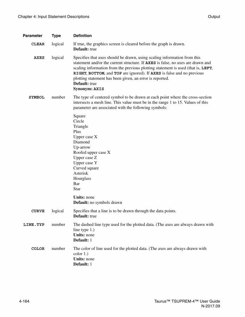
Chapter 4: Input Statement Descriptions Output

CLEAR logical If true, the graphics screen is cleared before the graph is drawn. Default: true

AXES logical Specifies that axes should be drawn, using scaling information from this statement and/or the current structure. If AXES is false, no axes are drawn and scaling information from the previous plotting statement is used (that is, LEFT, RIGHT, BOTTOM, and TOP are ignored). If AXES is false and no previous plotting statement has been given, an error is reported. Default: true Synonym: AXIS

SYMBOL number The type of centered symbol to be drawn at each point where the cross-section intersects a mesh line. This value must be in the range 1 to 15. Values of this parameter are associated with the following symbols:

SquareCircleTrianglePlusUpper case XDiamondUp-arrowRoofed upper case XUpper case ZUpper case YCurved squareAsteriskHourglassBarStar

Units: noneDefault: no symbols drawn

CURVE logical Specifies that a line is to be drawn through the data points.Default: true

LINE.TYP number The dashed line type used for the plotted data. (The axes are always drawn with line type 1.) Units: none Default: 1

COLOR number The color of line used for the plotted data. (The axes are always drawn with color 1.) Units: none Default: 1

Parameter Type Definition

4-164 Taurus™ TSUPREM-4™ User GuideN-2017.09

Output Chapter 4: Input Statement Descriptions

LEFT number The minimum value to be plotted on the x axis. Units: microns Default: minimum x or y coordinate of the structure Synonym: X.MIN

RIGHT number The maximum value to be plotted on the x axis. Units: microns Default: maximum x or y coordinate of the structure Synonym: X.MAX

BOTTOM number The minimum value of the selected expression to be plotted, in units of the plot variable. Units: units of the selected expression Default: minimum value of the selected expression Synonym: Y.MIN

TOP number The maximum value of the selected expression to be plotted, in units of the plot variable. Units: units of the selected expression Default: maximum value of the selected expression Synonym: Y.MAX

X.OFFSET number The distance by which the left end of the horizontal axis is offset from the left edge of the graphics viewport. Units: cm Default: 2.0

X.LENGTH number The length of the horizontal axis. Units: cm Default: viewport width - X.OFFSET - 1.25

X.SIZE number The height of the characters used to label the horizontal axis. Units: cm Default: 0.25

Y.OFFSET number The distance by which the bottom end of the vertical axis is offset from the bottom edge of the graphics viewport. Units: cm Default: 2.0

Y.LENGTH number The length of the vertical axis. Units: cm Default: viewport height - Y.OFFSET - 1.25

Y.SIZE number The height of the characters used to label the vertical axis. Units: cm Default: 0.25

T.SIZE number The height of the characters in the character string used as the plot title. Units: cm Default: 0.4

Parameter Type Definition

Taurus™ TSUPREM-4™ User Guide 4-165N-2017.09

Chapter 4: Input Statement Descriptions Output

Description The PLOT.1D statement plots cross-sections vertically or horizontally through the device, or along an interface between two materials, or along a boundary of the device. The statement has options to provide for initialization of the graphics device and plotting of axes. The statement can optionally draw vertical lines whenever a material boundary is crossed. The vertical axis corresponds to the variable selected with the SELECT statement.

Limits can be specified so that only a portion of the entire device is shown, or more than one variable can be conveniently plotted. By default the limits of the x axis extend to the edges of the structure, and the y axis is scaled according to the minimum and maximum values of the selected value over the entire structure.

The quantity to be plotted must be defined by a preceding SELECT statement. The type of graphics device must be set, either with an OPTION statement or through use of a suitable default. (See OPTION, p. 4-40 and Appendix B.)

If two materials are specified (for example, OXIDE /SILICON), a cross-section is plotted in the first material (for example, oxide) at the interface with the second material (for example, silicon). Note that OXIDE /SILICON produces different results from SILICON /OXIDE. For interface plots, the points along the interface are sorted by their x coordinates; specifying interfaces containing vertical segments or reentrant angles may not produce useful plots.

Line Type andColor

The LINE.TYP parameter specifies the dashed line type for plotting the data. Line type 1 is solid, while types 2 through 7 are dashed lines with increasing dash sizes. Types 8 through 10 produce more complicated patterns of dashes.

The COLOR parameter specifies the color for plotting the data. Color 1 is the default, and produces a line that contrasts with the background color (for example, black on white or white on black). The COLOR parameter has no effect on monochrome displays.

The colors produced by the COLOR parameter depend on the type of display being used. Where possible, the colors 2 through 7 have been set up to produce the colors red, green, blue, cyan (light blue), magenta (light purple), and yellow, in that order. Colors 8 and above produce a repeating series of 12 colors in rainbow order, from red to violet.

IN.FILE Parameter The format of the file specified by the IN.FILE parameter can be either columnwise or TIF. In the case of a columnwise format, the file may contain the following two types of lines:

1. Lines that are blank or contain a slash (/) as the first nonblank character are ignored and can be used to document the file.

2. Other lines define the data at one point in the distribution. These lines must contain the following values:

a. Value number X.COLUMN is the horizontal coordinate of the point.

b. Value number Y.COLUMN is the vertical coordinate of the point.

4-166 Taurus™ TSUPREM-4™ User GuideN-2017.09

Output Chapter 4: Input Statement Descriptions

If this line contains fewer than N numerical values in free-field format, where N is the maximum of indices (X.COLUMN and Y.COLUMN) for the values listed above, the line is ignored.

Since the .ivl log file of Medici is a TIF format file, the results of device simulation can be plotted if TIF, X.AXIS and Y.AXIS are specified. This capability makes it possible to easily compare the electrical calculations of TSUPREM-4 and Medici.

The transformation of data read by the IN.FILE parameter is as follows:

Data of X axis = X.SCALE x Data of X.COLUMN or X.AXIS + X.SHIFTData of Y axis = Y.SCALE x Data of Y.COLUMN or Y.AXIS + Y.SHIFT

Examples 1. The following statement clears the screen, draws a set of axes, and plots a (vertical) cross-section at x=1.0 micron:

PLOT.1D X.V=1.0 SYMB=1 ^CURVE

Symbol 1 (a small square) is drawn at each data point; the line through the data points is suppressed.

2. The following statement plots a cross-section at x=2.0 microns on the previous set of axes, without clearing the screen:

PLOT.1D X.V=2.0 ^AXES ^CLEAR LINE.TYP=2 COLOR=3

A line consisting of short dashes is used, and appears in color 3 on color displays.

Taurus™ TSUPREM-4™ User Guide 4-167N-2017.09

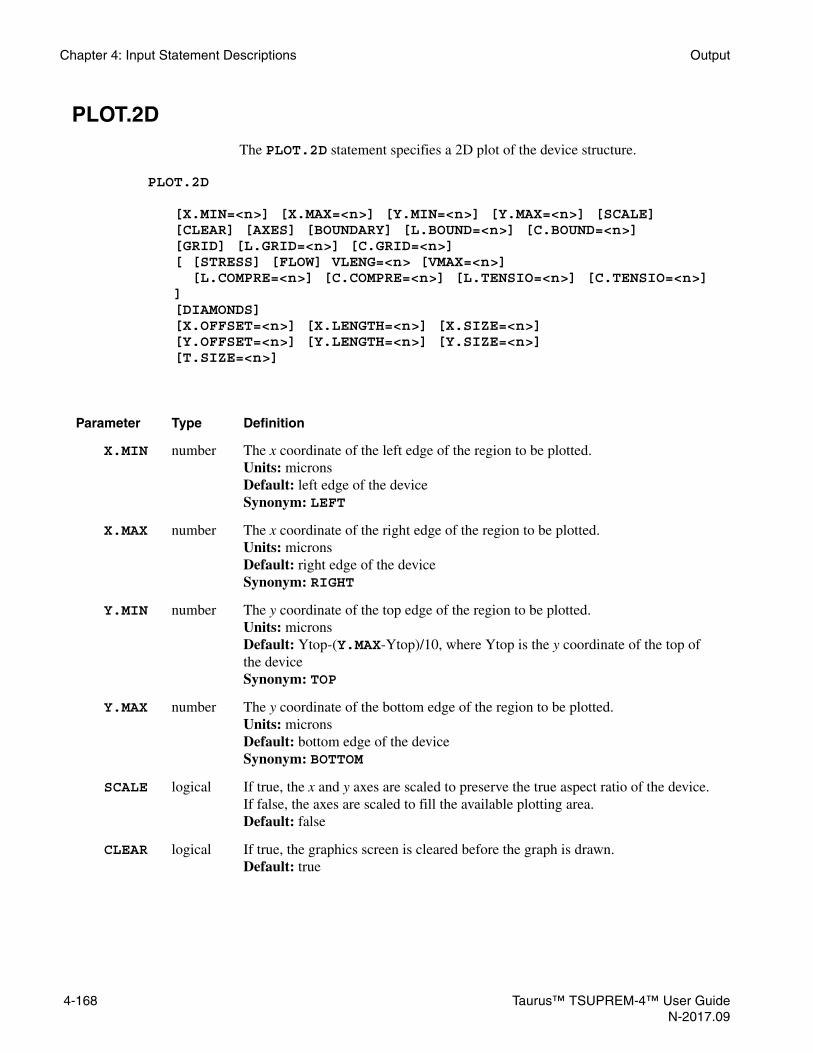
Chapter 4: Input Statement Descriptions Output

PLOT.2D

The PLOT.2D statement specifies a 2D plot of the device structure.

PLOT.2D [X.MIN=<n>] [X.MAX=<n>] [Y.MIN=<n>] [Y.MAX=<n>] [SCALE] [CLEAR] [AXES] [BOUNDARY] [L.BOUND=<n>] [C.BOUND=<n>] [GRID] [L.GRID=<n>] [C.GRID=<n>] [ [STRESS] [FLOW] VLENG=<n> [VMAX=<n>] [L.COMPRE=<n>] [C.COMPRE=<n>] [L.TENSIO=<n>] [C.TENSIO=<n>] ] [DIAMONDS] [X.OFFSET=<n>] [X.LENGTH=<n>] [X.SIZE=<n>] [Y.OFFSET=<n>] [Y.LENGTH=<n>] [Y.SIZE=<n>] [T.SIZE=<n>]

Parameter Type Definition

X.MIN number The x coordinate of the left edge of the region to be plotted. Units: microns Default: left edge of the device Synonym: LEFT

X.MAX number The x coordinate of the right edge of the region to be plotted. Units: microns Default: right edge of the device Synonym: RIGHT

Y.MIN number The y coordinate of the top edge of the region to be plotted. Units: microns Default: Ytop-(Y.MAX-Ytop)/10, where Ytop is the y coordinate of the top of the device Synonym: TOP

Y.MAX number The y coordinate of the bottom edge of the region to be plotted. Units: microns Default: bottom edge of the device Synonym: BOTTOM

SCALE logical If true, the x and y axes are scaled to preserve the true aspect ratio of the device. If false, the axes are scaled to fill the available plotting area. Default: false

CLEAR logical If true, the graphics screen is cleared before the graph is drawn. Default: true

4-168 Taurus™ TSUPREM-4™ User GuideN-2017.09

Output Chapter 4: Input Statement Descriptions

AXES logical Specifies that axes should be drawn, using scaling information from this statement and/or the current structure. If AXES is false, no axes are drawn and scaling information from the previous plotting statement is used (that is, X.MIN, X.MAX, Y.MIN, and Y.MAX are ignored). If AXES is false and no previous plotting statement has been given, an error is reported. Default: true Synonym: AXIS

BOUNDARY logical Plot the device boundary and material interfaces. Default: true

L.BOUND number The dashed line type used for plotting the device boundary and material interfaces. Units: none Default: 1 Synonyms: LINE.BOU, LINE.TYP

C.BOUND number The line color used for plotting the device boundary and material interfaces. Units: none Default: 1

GRID logical Plot the grid used for the numerical solution. Default: false

L.GRID number The dashed line type used for plotting the grid. Units: none Default: 1 Synonym: LINE.GRI

C.GRID number The line color used for plotting the grid.Units: none Default: 1

STRESS logical Plot the principal stresses in the structure. Vectors are drawn along the two principal axes of the stress tensor at each mesh point.Default: false

FLOW logical Plot vectors indicating the velocity (due to oxidation) or displacement (calculated by the STRESS statement) at each mesh point.Default: false

VLENG number The length of the vector drawn for the maximum value of stress or velocity.Units: micronsDefault: none

VMAX number The maximum value of stress or velocity to be plotted.Units: dynes/cm2 for stress, cm/s for flowDefault: no limit on maximum value

Parameter Type Definition

Taurus™ TSUPREM-4™ User Guide 4-169N-2017.09

Chapter 4: Input Statement Descriptions Output

L.COMPRE number The dashed line type used for plotting compressive stress vectors and flow vectors. Units: none Default: 1 Synonyms: L.FLOW, L.VELOCI, LINE.COM

C.COMPRE number The line color used for plotting compressive stress vectors and flow vectors. Units: none Default: 1 Synonyms: C.FLOW, C.VELOCI

L.TENSIO number The dashed line type used for plotting tensile stress vectors. Units: none Default: 1 Synonym: LINE.TEN

C.TENSIO number The line color used for plotting tensile stress vectors. Units: none Default: 1

DIAMONDS logical Plot a small symbol at each mesh point location. Default: false

X.OFFSET number The distance by which the left end of the horizontal axis is offset from the left edge of the graphics viewport. Units: cm Default: 2.0

X.LENGTH number The length of the horizontal axis. Units: cm Default: viewport width - X.OFFSET - 1.25

X.SIZE number The height of the characters used to label the horizontal axis. Units: cm Default: 0.25

Y.OFFSET number The distance by which the bottom end of the vertical axis is offset from the bottom edge of the graphics viewport. Units: cm Default: 2.0

Y.LENGTH number The length of the vertical axis. Units: cm Default: viewport height - Y.OFFSET - 1.25

Parameter Type Definition

4-170 Taurus™ TSUPREM-4™ User GuideN-2017.09

Output Chapter 4: Input Statement Descriptions

Description The PLOT.2D statement specifies a 2D plot. It is useful in itself for plotting structure outlines and interface locations, grid, stress, and velocities. It is also used to plot axes for the CONTOUR and COLOR statements.

The type of graphics device must be set, either with an OPTION statement or use of a suitable default. See OPTION, p. 4-40 and Appendix B.

The x and y limits are in microns, and refer to the coordinates of the structure being simulated. The x coordinate increases from left to right on the plot, while y increases from top to bottom. If Y.MIN is greater than Y.MAX, the plot is flipped. Thus, the value at the top of the plot (Y.MIN) is greater than the value at the bottom of the plot (Y.MAX). Similarly, X.MIN can be greater than X.MAX.

For STRESS and FLOW plots, the maximum vector length must be given by VLENG. VLENG is in the same units as the device structure, namely microns. If VMAX is specified, values of stress or velocity larger than the specified value are not plotted.

Line Type andColor

The L.BOUND, L.GRID, L.COMPRE, and L.TENSIO parameters specify dashed line types to be used for plotting various quantities. Type 1 produces a solid line while types 2 through 10 produce various dashed line styles.

The C.BOUND, C.GRID, C.COMPRE, and C.TENSIO parameters specify the colors to be used in plotting the various quantities. Color 1 (the default) gives a line color that contrasts with the background (for example, black on white or green on black). Colors 2 through 7 give red, green, blue, cyan (light blue), magenta (light purple), and yellow on most displays, while colors 8 and above produce a repeating sequence of 12 colors in rainbow order from red to violet. Note that not all display types give these colors; the color parameters have no effect on monochrome displays.

Examples 1. The following statement plots the axes, triangular grid, and structure boundaries (in that order):

PLOT.2D SCALE GRID C.GRID=2

The grid is plotted with color 2 (usually red on color devices). The plot is scaled the same in the x and y directions to display the correct aspect ratio of the structure.

Y.SIZE number The height of the characters used to label the vertical axis. Units: cm Default: 0.25

T.SIZE number The height of the characters in the character string used as the plot title. Units: cm Default: 0.4

Parameter Type Definition

Taurus™ TSUPREM-4™ User Guide 4-171N-2017.09

Chapter 4: Input Statement Descriptions Output

2. The following statement draws the material interfaces and axis between 2.0 and 5.0 microns, without clearing the screen first:

PLOT.2D X.MIN=2 X.MAX=5 SCALE ^CLE

The plot is scaled to show the true aspect ratio of the structure.

3. The following statement draws the structure boundaries and material interfaces using line type 2, and shows the grid points as diamonds:

PLOT.2D LINE.TYP=2 DIAMONDS ^AXES ^CLEAR

The plotting area is not cleared, and axes from the previous plot are used. The aspect of the structure can be distorted because SCALE is not specified.

4-172 Taurus™ TSUPREM-4™ User GuideN-2017.09

Output Chapter 4: Input Statement Descriptions

CONTOUR

The CONTOUR statement plots a contour of the selected variable on a 2D plot.

CONTOUR VALUE=<n> [LINE.TYP=<n>] [COLOR=<n>] [SYMBOL=<n>]

Parameter Type Definition

VALUE number The value of the selected variable at which to plot a contour. Units: units of the selected variableDefault: none

LINE.TYP number The dashed line type to be used for the contour. Units: noneDefault: 1

COLOR number The line color to be used for the contour. Units: noneDefault: 1

SYMBOL number The type of centered symbol to be drawn at each mesh line intersection on the contour. This value must be in the range 1 to 15. Values of this parameter are associated with the following symbols:SquareCircleTrianglePlusUpper case XDiamondUp-arrowRoofed upper case XUpper case ZUpper case YCurved squareAsteriskHourglassBarStarUnits: noneDefault: no symbols drawn

Taurus™ TSUPREM-4™ User Guide 4-173N-2017.09

Chapter 4: Input Statement Descriptions Output

Description The CONTOUR statement draws a contour of the selected variable at the value specified. The value must be specified in units of the selected variable.

This statement assumes that a PLOT.2D statement has been specified previously and the screen has been set up for plotting a 2D picture. The variable to be plotted must have been specified on a preceding SELECT statement.

Note:The results of this statement are undefined unless valid PLOT.2D and SELECT statements have been executed beforehand.

Line Type andColor

Line type 1 gives a solid line, while types 2 through 10 give dashed lines of various sorts. Color 1 produces contours that contrast with the background (for example, black on white or green on black). On most color devices, colors 2 through 7 give red, green, blue, cyan (light blue), magenta (light purple), and yellow, while colors 8 and above give a repeating series of 12 colors in rainbow order (from red to violet). On monochrome devices, the COLOR parameter has no effect.

Example The following statements plot a series of contours with line type 2, where the boron concentration is equal to 1015, 1016, 1017, 1018, and 1019:

SELECT Z=log10(Boron)FOREACH X ( 15 TO 19 STEP 1 )

CONTOUR VALUE=X LINE.TYP=2END

Note the use of the CONTOUR statement inside a FOREACH loop, to plot a series of contours.

AdditionalCONTOUR Notes

• Values of contours of log10(concentration) should be specified as exponents, for example, 16 and not 1e16.

• Symbols are placed where the contour crosses a boundary between mesh elements. Thus, the density of symbols reflects the density of the mesh along a contour.

4-174 Taurus™ TSUPREM-4™ User GuideN-2017.09

Output Chapter 4: Input Statement Descriptions

COLOR

The COLOR statement fills an area of a 2D plot.

COLOR [COLOR=<n>] [MIN.VALU=<n>] [MAX.VALU=<n>] [ { MATERIAL=<c> | SILICON | OXIDE | OXYNITRI | NITRIDE | POLYSILI | ALUMINUM | PHOTORES } ]

Parameter Type Definition

COLOR number The “color” to be used for the area fill. This can correspond to an actual color, a shade of gray, or to a fill pattern, depending on the plot device. Units: noneDefault: 1

MIN.VALU number The minimum value of the selected variable to be filled.Units: units of the selected variableDefault: the minimum value of the selected variable

MAX.VALU number The maximum value of the selected variable to be filled.Units: units of the selected variableDefault: the maximum value of the selected variable

MATERIAL character Only regions of the named material are filled.Default: none

SILICON logical Only regions of the device composed of silicon are filled. Default: false

OXIDE logical Only regions of the device composed of oxide are filled. Default: false

OXYNITRI logical Only regions of the device composed of oxynitride are filled. Default: false

NITRIDE logical Only regions of the device composed of nitride are filled. Default: false

POLYSILI logical Only regions of the device composed of polysilicon are filled. Default: false

ALUMINUM logical Only regions of the device composed of aluminum are filled. Default: false

PHOTORES logical Only regions of the device composed of photoresist are filled. Default: false

Taurus™ TSUPREM-4™ User Guide 4-175N-2017.09

Chapter 4: Input Statement Descriptions Output

Description The COLOR statement performs area fills on isoconcentration bands in the selected variable. If either the MIN.VALU or MAX.VALU keyword is specified, regions of the device having values of the plot variable between the two values are filled. If a material type is specified, only regions of the structure composed of the specified material are filled. If neither MIN.VALU or MAX.VALU is specified, all regions of the specified material are filled. If no values or materials are specified, a warning is printed and the statement is ignored.

The quantity referred to by MIN.VALU and MAX.VALU must be specified on a SELECT statement preceding the COLOR statement. The axes for the plot must be set up by a preceding PLOT.2D statement.

Plot DeviceSelection

The effect of the COLOR statement depends on the type of plot device selected. On color devices, the specified areas are colored. In most cases, colors 2 through 7 are red, green, blue, cyan (light blue), magenta (light purple), and yellow, while colors 8 and above produce a repeating series of 12 colors in rainbow order (red to violet). On some monochrome devices, different values of COLOR produce varying gray-scale or halftone values. On devices without hardware area fill capabilities (defined in the s4pcap file), a cross-hatch pattern is used.

On some devices an area fill may overwrite previously plotted information, such as grid or material boundaries. In this case the grid or boundaries can be re-plotted after doing the area fill, to ensure that they are visible.

Examples 1. The following statement fills all oxide regions with color 4:

COLOR OXIDE COLOR=4

2. The following statements fill those portions of the structure having a boron concentration between 1015 and 1016 with color:

SELECT Z=log10(Boron)COLOR MIN.V=15 MAX.V=16 COLOR=3

4-176 Taurus™ TSUPREM-4™ User GuideN-2017.09

Output Chapter 4: Input Statement Descriptions

PLOT.3D

Create a 3D projection plot of the solution.

PLOT.3D [THETA=<n>] [PHI=<n>] [CLEAR] [X.MIN=<n>] [X.MAX=<n>] [Y.MIN=<n>] [Y.MAX=<n>] [Z.MIN=<n>] [Z.MAX=<n>] [LINE.TYP=<n>] [COLOR=<n>] [NUM.CNTR=<n>] [BOUNDARY] [L.BOUND=<n>] [C.BOUND=<n>]

Parameter Type Definition

THETA number The angle above the x-y plane from which the device is viewed. If an angle of 0 is specified, the viewpoint is in the x-y plane. Values between –90 and 90 are permitted. Units: degrees Default: 45 Synonym: ELEVATIO

PHI number The angle of counter-clockwise rotation of the device in the x-y plane. Only values within 30 degrees of 45, 135, 225, and 315 degrees should be used; values outside this range are not supported. Never use values of 0, 90, 180, or 270 degrees. Units: degrees Default: 45 Synonym: AZIMUTH

CLEAR logical Specifies that the graphics display area is to be cleared before beginning the plot. Default: true

X.MIN number The minimum value to be plotted along the x axis. Units: microns Default: the minimum x coordinate of the current structure

X.MAX number The maximum value to be plotted along the x axis. Units: microns Default: the maximum x coordinate of the current structure

Y.MIN number The minimum value to be plotted along the y axis. Units: microns Default: the minimum y coordinate of the current structure

Y.MAX number The maximum value to be plotted along the y axis. Units: microns Default: the maximum y coordinate of the current structure

Taurus™ TSUPREM-4™ User Guide 4-177N-2017.09

Chapter 4: Input Statement Descriptions Output

Description The PLOT.3D statement plots a “bird’s eye view” of a three-dimensional wire diagram of the selected data. The routine interpolates a series of cross-section lines and plots them with the given viewpoint parameters. Axes can be drawn and labeled.

The variable to be plotted must be specified with a SELECT statement prior to the PLOT.3D statement. The graphics device to be used must be set with an OPTION statement, unless an appropriate default device is available.

Note:The algorithms used work only for certain values of PHI; values near 0°, 90°, 180°, or 270° should be avoided.

Z.MIN number The minimum value on the z axis. Units: units of the plot variable Default: the minimum value of the plot variable

Z.MAX number The maximum value on the z axis. Units: units of the plot variable Default: the maximum value of the plot variable

LINE.TYP number The dashed line type to be used for plotting the data. Units: noneDefault: 1

COLOR number The line color to be used for plotting the data. Units: noneDefault: 1

NUM.CNTR number The number of grid lines drawn to represent the surface. One axis has this number of lines, the other is drawn with a number calculated from it dependent on the value of PHI. Units: noneDefault: 20

BOUNDARY logical Draw the device boundaries on the z=Z.MIN plane of the plot. Default: true

L.BOUND number The dashed line type used for plotting the boundary. Units: noneDefault: 1 Synonym: LINE.BOU

C.BOUND number The line color used for plotting the boundary. Units: noneDefault: 1

Parameter Type Definition

4-178 Taurus™ TSUPREM-4™ User GuideN-2017.09

Output Chapter 4: Input Statement Descriptions

Line Type andColor

The LINE.TYP and L.BOUND parameters specify the style of dashed line to be used for plotting the data and boundaries, respectively. Type 1 produces a solid line, while types 2 through 10 produce various dashed styles.

The COLOR and C.BOUND parameters specify the color of lines to be used for data and boundaries. Color 1 produces lines that contrast with the background (for example, black on white or green on black). On most color displays, colors 2 through 7 give red, green, blue, cyan (light blue), magenta (light purple), and yellow, while colors 8 and above give a repeating sequence of 12 colors in rainbow order (red through violet).

Examples 1. The following statement plots the device as viewed from straight above:

PLOT.3D NUM.C=30 THETA=90

Thirty contour lines are selected.

2. The following statement plots the bird’s eye view plot from 60 deg above the horizon and 30 deg off the x axis:

PLOT.3D PHI=30 THETA=60 COLOR=4

Color 4 (usually blue) is used.

Additional PLOT.3DNotes

• Nonrectangular areas are padded with Z.MIN values to make the final surface rectangular.

• Z.MIN and Z.MAX specify the limits of the z axis, but values being plotted are not clipped at these values.

Taurus™ TSUPREM-4™ User Guide 4-179N-2017.09

Chapter 4: Input Statement Descriptions Output

LABEL

The LABEL statement is used to add a label to a plot.

LABEL

{ ( X=<n> Y=<n> [CM] ) | ( [X.CLICK=<c>] [Y.CLICK=<c>] ) }[SIZE=<n>] [COLOR=<n>]

[ LABEL=<c> [ {LEFT | CENTER | RIGHT} ] ] [LINE.TYP=<n>] [C.LINE=<n>] [LENGTH=<n>] [ { ( [SYMBOL=<n>] [C.SYMBOL=<n>] ) | ( [RECTANGL] [C.RECTAN=<n>] [W.RECTAN=<n>] [H.RECTAN=<n>] ) } ]

Parameter Type Definition

X number The horizontal location corresponding to the left end, center, or right end of the character string (depending on whether LEFT, CENTER, or RIGHT is specified). If the CM parameter is specified, then this parameter specifies a location in centimeters relative to the left edge of the graphics viewport. Otherwise, this parameter specifies the location in axis units along the horizontal axis. Units: cm or horizontal axis units Default: none

Y number The vertical location corresponding to the bottom of the character string. If the CM parameter is specified, then this parameter specifies a location in centimeters relative to the bottom edge of the graphics viewport. Otherwise, this parameter specifies the location in axis units along the vertical axis. Units: cm or vertical axis units Default: none

CM logical Specifies that the X and Y parameters are locations in centimeters relative to the lower left edge of the graphics viewport. Default: false

X.CLICK character The variable name to store the x-coordinate of the position at which a mouse is clicked.Units: horizontal axis units Default: none

Y.CLICK character The variable name to store the y-coordinate of the position at which a mouse is clicked.Units: cm or vertical axis units Default: none

4-180 Taurus™ TSUPREM-4™ User GuideN-2017.09

Output Chapter 4: Input Statement Descriptions

SIZE number The height of the characters in the character string, and the default size to be used for rectangles and centered symbols. Units: cm Default: 0.25 Synonym: C.SIZE

COLOR number The color of the label text, and the default color for rectangles, centered symbols, and line segments. Units: noneDefault: 1

LABEL character The character string to be used to label the plot. Default: none

LEFT logical Specifies that the character string is to start at the position given by X and Y. Default: true if neither CENTER or RIGHT is true

CENTER logical Specifies that the character string is to be centered horizontally about the position given by X and Y. Default: false

RIGHT logical Specifies that the character string is to end at the position given by X and Y. Default: false

LINE.TYP number The dashed type of a line segment to be plotted before the label. If LABEL is not specified, the line segment is centered at the point given by X and Y.Units: noneDefault: 1

C.LINE number The color of the line segment to be plotted before the label. Units: noneDefault: COLOR

LENGTH number The length of the line segment to be plotted before the label. Units: cm Default: 4*SIZE

Parameter Type Definition

Taurus™ TSUPREM-4™ User Guide 4-181N-2017.09

Chapter 4: Input Statement Descriptions Output

SYMBOL number The type of centered symbol to be drawn before the label. This value must be in the range 1 to 15. Values of this parameter are associated with the following symbols:SquareCircleTrianglePlusUpper case XDiamondUp-arrowRoofed upper case XUpper case ZUpper case YCurved squareAsteriskHourglassBarStar

If LABEL is specified, the symbol is placed to the left of the label with one character space between the symbol and the label text. If LABEL is not specified, the rectangle is centered at the point given by X and Y.Units: noneDefault: 1

C.SYMBOL number The color of the symbol (if any). Units: noneDefault: COLOR

RECTANGL logical Specifies that a filled rectangle be plotted with the label. If LABEL is specified, the rectangle is placed to the left of the label with one character space between the rectangle and the label text. If LABEL is not specified, the rectangle is centered at the point given by X and Y. Default: false

C.RECTAN number The color of the filled rectangle. Units: noneDefault: COLOR

W.RECTAN number The width of the filled rectangle. Units: cm Default: SIZE

H.RECTAN number The height of the filled rectangle. Units: cm Default: SIZE

Parameter Type Definition

4-182 Taurus™ TSUPREM-4™ User GuideN-2017.09

Output Chapter 4: Input Statement Descriptions

Description The LABEL statement is used to add text, symbols, and/or filled rectangles to a plot. This statement is meaningless unless a PLOT.1D, PLOT.2D, or PLOT.3D statement has been previously specified.

Label Placement The rules for placing these annotations are as follows:

1. Labels are always placed at the location specified by X and Y. The label is left justified, centered, or right justified at this location, depending on whether LEFT, CENTER, or RIGHT is specified.

2. The placement of line segments depends on whether a LABEL is specified:

a. If a LABEL is specified, the line segment is placed one character width to the left of the label.

b. If no LABEL is specified, the line segment is centered at the location specified by X and Y.

3. The placement of symbols and filled rectangles depends on whether a line segment or label is specified:

a. If a line segment is specified, the symbol or filled rectangle is centered on the line segment.

b. If no line segment is specified but a LABEL is specified, the symbol or filled rectangle is placed one character width to the left of the label.

c. If neither a line segment nor a LABEL is specified, the symbol or filled rectangle is centered at the location specified by X and Y.

4. The coordinates X and Y should be in the units of the plot axes, for example, microns or 1/cm3, unless CM is specified.

Note:Some graphics devices have a cursor whose position can be read by the program. On such devices, a LABEL statement without X and Y coordinates attempts to read the cursor position and plot the label at that point. On terminals from which the cursor position cannot be read, a LABEL statement without X and Y coordinates may produce unpredictable results.

Line, Symbol,and Rectangle

If LINE.TYP, C.LINE, or LENGTH is specified, a line segment is drawn. LINE.TYP specifies the dashed line type of the line segment. Type 1 produces a solid line, while types 2 through 10 produce various styles of dashed lines. C.LINE specifies the color of the line and LENGTH gives the length. If either SYMBOL or C.SYMBOL is specified, a symbol is drawn. If RECTANGL, C.RECTAN, W.RECTAN, or H.RECTAN is specified, a filled rectangle is drawn.

The SIZE parameter specifies the character size to be used for the label and the default width and height for filled rectangles.

Taurus™ TSUPREM-4™ User Guide 4-183N-2017.09

Chapter 4: Input Statement Descriptions Output

Color The COLOR parameter specifies the color to be used for the label and the default color for any line segment, symbol, or filled rectangle. Color 1 contrasts with the background (for example, black on white or white on black). On most color devices, colors 2 through 7 produce red, green, blue, cyan (light blue), magenta (light purple), and yellow, while colors 8 and above give a repeating sequence of 12 colors in rainbow order (red through violet). The COLOR parameter has no effect on monochrome devices.

Examples 1. The following statements put two labels on the plot starting at x=3 microns and y=1.4 and 1.6 microns, with a short line of the specified type before each one:

LABEL X=3.0 Y=1.4 LABEL="Arsenic" LINE=3LABEL X=3.0 Y=1.6 LABEL="Phosphorus" LINE=4

2. The following statement plots a label preceded by a filled rectangle:

LABEL RIGHT X=12.5 Y=9.0 CM LABEL="Oxide" C.RECT=2

The label ends at a point 12.5 cm from the x axis and 9.0 cm from the y axis. It is preceded by a rectangle filled with color 2.

3. The following statement stores the coordinate of the position at which a mouse is clicked:

LABEL LABEL=x X.CLICK=px Y.CLICK=py

The variables, px, py store the coordinate of the position at which a mouse is clicked.

Note:The unit of the stored value in X.CLICK is the same as the x-coordinate unit. However, in the case of Y.CLICK, the unit is cm for the distance. In PLOT.2D graph, for example, the variable of Y.CLICK stores the y-coordinate value in cm unit, while the variable of X.CLICK value stores the x-coordinate value in um unit.

4-184 Taurus™ TSUPREM-4™ User GuideN-2017.09

Output Chapter 4: Input Statement Descriptions

EXTRACT

The EXTRACT statement extracts information about the structure, prints the results, and/or writes them to a file.

EXTRACT [ {MATERIAL=<c> | SILICON | OXIDE | OXYNITRI | NITRIDE | POLYSILI | PHOTORES | ALUMINUM} ] [P1.X=<n>] [P1.Y=<n>] [P2.X=<n>] [P2.Y=<n>] [ {/MATERIA=<c> | /SILICON | /OXIDE | /OXYNITR | /NITRIDE | /POLYSIL | /PHOTORE | /ALUMINU | /AMBIENT} [CLOCKWIS] ] [X=<n>] [Y=<n>] [ {DISTANCE=<n> | MINIMUM | MAXIMUM | VALUE=<n>} ] { ( [X.EXTRAC] [Y.EXTRAC] [D.EXTRAC] [VAL.EXTR] ) | ( [INT.EXTR] [AREA.EXT] [AVG.EXTR] ) } [PREFIX=<c>] [SEPARAT=<c>] [SUFFIX=<c>] [WRITE] [PRINT] [ NAME=<c> [ASSIGN] [ { TARGET=<n> | ( T.FILE=<c> [V.COLUMN=<n>] [V.LOWER=<n>] [V.UPPER=<n>] [T.COLUMN=<n>] [T.LOWER=<n>] [T.UPPER=<n>] [V.TRANSF=<c>] [T.TRANSF=<c>] [Z.VALUE=<c>] [SENSITIV]) } [TOLERANC=<n>] [WEIGHT=<n>]

[MIN.REL=<n>] [MIN.ABS=<n>]]

] [ OUT.FILE=<c> [APPEND] ] [CLOSE]

Parameter Type Definition

MATERIAL character Extract parameters in the named material.Default: none

SILICON logical Extract parameters in silicon.Default: false

OXIDE logical Extract parameters in oxide.Default: false

OXYNITRI logical Extract parameters in oxynitride.Default: false

NITRIDE logical Extract parameters in nitride.Default: false

POLYSILI logical Extract parameters in polysilicon.Default: falseSynonym: POLY

Taurus™ TSUPREM-4™ User Guide 4-185N-2017.09

Chapter 4: Input Statement Descriptions Output

PHOTORES logical Extract parameters in photoresist.Default: false

ALUMINUM logical Extract parameters in aluminum.Default: false

P1.X number The x coordinate of the starting point of a line through the structure.Units: microns Default: the left edge of the structure if an interface is specified, or 0.0, otherwise

P1.Y number The y coordinate of the starting point of a line through the structure.Units: microns Default: 0.0 if an interface is specified, or the top of the structure otherwise

P2.X number The x coordinate of the end point of a line through the structure.Units: microns Default: the right edge of the structure, or P1.X otherwise

P2.Y number The y coordinate of the end point of a line through the structure.Units: microns Default: 0.0 if an interface is specified, or the bottom of the structure, otherwise

/MATERIA character Extract parameters along the interface with the named material.Default: none

/SILICON logical Extract parameters along the interface with silicon.Default: false

/OXIDE logical Extract parameters along the interface with oxide.Default: false

/OXYNITR logical Extract parameters along the interface with oxynitride.Default: false

/NITRIDE logical Extract parameters along the interface with nitride.Default: false

/POLYSIL logical Extract parameters along the interface with polysilicon.Default: false

/PHOTORE logical Extract parameters along the interface with photoresist.Default: false

/ALUMINU logical Extract parameters along the interface with aluminum.Default: false

/AMBIENT logical Extract parameters along exposed surfaces.Default: falseSynonyms: /EXPOSED, /GAS

Parameter Type Definition

4-186 Taurus™ TSUPREM-4™ User GuideN-2017.09

Output Chapter 4: Input Statement Descriptions

CLOCKWIS logical If the specified material interface forms a closed loop, traverse it in the clockwise direction.Default: false

X number Define a line or a point on a line by the value of its x coordinate.Units: micronsDefault: none

Y number Define a line or a point on a line by the value of its y coordinate.Units: microns Default: 0.0

DISTANCE number Define a point on a line by its distance from the start of the line.Units: microns Default: 1.0

MINIMUM logical Extract at the first point on a line where the value of the selected variable is at its minimum.Default: false

MAXIMUM logical Extract at the first point on a line where the value of the selected variable is at its maximum.Default: false

VALUE number Extract at the first point on a line where the selected variable has the specified value.Units: the units of the selected variableDefault: none

X.EXTRAC logical Extract the x coordinate of the specified point.Default: false

Y.EXTRAC logical Extract the y coordinate of the specified point.Default: false

D.EXTRAC logical Extract the distance of the specified point from the start of the specified line.Default: false

VAL.EXTR logical Extract the value of the selected variable at the specified point.Default: false

INT.EXTR logical Extract the integral of the selected variable along the specified line.Default: falseSynonym: INTEGRAL

AREA.EXT logical Extract the length of the specified line.Default: falseSynonym: THICKNES

AVG.EXTR logical Extract the average value of the selected variable along the specified line.Default: false

Parameter Type Definition

Taurus™ TSUPREM-4™ User Guide 4-187N-2017.09

Chapter 4: Input Statement Descriptions Output

PREFIX character A character string to be printed before the extracted value(s). Note that if a space is desired before the first value, it must be explicitly specified as part of the prefix.Default: none

SEPARAT character A character string to be printed between extracted values if more than value is extracted.Default: " " (a single space)

SUFFIX character A character string to be printed after the extracted value(s). Note that if a space is desired after the last value, it must be explicitly specified as part of the suffix.Default: none

WRITE logical Specifies that the extracted result is to be written to the extract output file, if one is open.Default: true

PRINT logical Specifies that the extracted result is to be printed on the standard output (including the output listing file and the user’s terminal).Default: true

NAME character Specifies that the extracted result is to be assigned to the specified name, as if it had been defined with a DEFINE statement or an ASSIGN statement when either TARGET or T.FILE is specified. Note that if the specified name has been defined with a DEFINE statement previously, you need to precede the EXTRACT statement with a “%” (percent character) to prevent substitution of its previous value. The NAME parameter allows extracted results to be used in subsequent extractions or simulations.Default: none

ASSIGN logical Specifies that the extracted quantity to be assigned to the variable specified by NAME is the same style as the ASSIGN statement.Default: false

TARGET number The desired value of the target being defined for an optimization loop. The optimization attempts to match the extracted value with the value of this parameter.Units: determined by the extracted valuesDefault: none

T.FILE character The file name containing the desired values of the target being defined for an optimization loop. The desired values are in the column specified by the T.COLUMN parameter. The optimization attempts to match the extracted values with the desired values.Default: none

V.COLUMN number The index of the column in the file specified by the T.FILE parameter, which contains the variable at which the extraction is performed.Units: noneDefault: 1

Parameter Type Definition

4-188 Taurus™ TSUPREM-4™ User GuideN-2017.09

Output Chapter 4: Input Statement Descriptions

V.LOWER number The lower limit of the variable to be read from T.FILE. The target data at variable values less than the value of V.LOWER parameter are excluded during an optimization loop. Note that the V.LOWER specifies the value prior to the transformation by V.TRANSF.Units: The same as the unit of variable specified by V.COLUMNDefault: -1e+30

V.UPPER number The upper limit of the variable to be read from T.FILE. The target data at variable values greater than the value of V.UPPER parameter are excluded during an optimization loop. Note that the V.UPPER specifies the value prior to the transformation by V.TRANSF.Units: the same as the unit of variable specified by V.COLUMNDefault: 1e+30

T.COLUMN number The index of the column in the file specified by the T.FILE parameter, which contains the desired values of the target being defined for an optimization loop.Units: noneDefault: 2

T.LOWER number The lower limit of the desired value of a target to be read from T.FILE. Target values less than the value of T.LOWER parameter are excluded during an optimization loop. Note that the T.LOWER specifies the value prior to the transformation by T.TRANSF.Units: the same as the unit of variable specified by T.COLUMNDefault: -1e+30

T.UPPER number The upper limit of the desired value of a target to be read from T.FILE. Target values greater than the value of T.UPPER parameter are excluded during an optimization loop. Note that the T.UPPER specifies the value prior to the transformation by T.TRANSF.Units: the same as the unit of variable specified by T.COLUMNDefault: 1e+30

V.TRANSF character The function for transformation of the variable data read from T.FILE. The specified character string represents the function of a variable V, with which the variable data specified by V.COLUMN parameter are transformed.Default: none

T.TRANSF character The function for transformation of the desired data of a target read from T.FILE. The specified character string represents the function of a variable T, with which the target data specified by T.COLUMN parameter are transformed.Default: none

Z.VALUE character The function which generates the data instead of simulation. The specified character string represents a function of the variable V, which corresponds to the variable specified by V.COLUMN parameter.Units: the same as the unit of target data specified by T.COLUMNDefault: none

Parameter Type Definition

Taurus™ TSUPREM-4™ User Guide 4-189N-2017.09

Chapter 4: Input Statement Descriptions Output

Description The EXTRACT statement is used to extract values along a line through a structure or at a point. It has the following properties and uses:

• When a line is specified, layer thicknesses and integrals and averages of solution values can be extracted.

• Lines through the structure can be vertical, horizontal, or oblique; material interfaces can also be treated as lines for purposes of extraction.

TOLERANC number The RMS (root-mean-square) error for convergence criterion. An optimization loop terminates when the RMS errors of all of specified targets are smaller than TOLERANC.Units: %Default: 0.0

SENSITIV logical Specifies the plot of sensitivity analysis of the target defined by this EXTRACT statement. This parameter works only if the PLOT parameter in the LOOP statement is true. Default: true

WEIGHT number The weighting factor applied to the target being defined for an optimization loop. The weights are used to control the importance of individual targets in calculations of the error during optimization.Units: noneDefault: 1.0

MIN.REL number The minimum target ratio for which relative error is used to calculated the error during optimization. This value is compared with the ratio of the absolute target value to the maximum absolute target value defined by this EXTRACT statement. Units: noneDefault: 1e-10

MIN.ABS number The minimum target value for which relative error is used to calculate the error during optimization. This value is compared with the absolute target value. Units: determined by the extracted valuesDefault: 1e-10

OUT.FILE character The name of an extract output file to be opened. The file is opened before extracting any values, so extracted results appear in the file.Default: none

APPEND logical Specifies that extracted values are to be appended to the file specified by the OUT.FILE parameter. If APPEND is false, any existing data in the specified file is discarded when the file is opened.Default: false

CLOSE logical Specifies that the extract output file is to be closed. The file is closed after any values extracted by this EXTRACT statement are written.Default: false

Parameter Type Definition

4-190 Taurus™ TSUPREM-4™ User GuideN-2017.09

Output Chapter 4: Input Statement Descriptions

• When a point is specified, the solution value, the coordinates of the point, and the distance from the start of a line can be extracted.

• Points can be specified by their coordinates or by the distance from the start of a line. You can also request extraction at the point at which the solution value is a minimum or maximum or takes on a specified value.

• Extraction can be limited to regions of specified materials, or can encompass the entire structure.

• Extracted results can be printed on the standard output or written to a separate output file. Text surrounding and between extracted values can be specified by you.

• Parameters are available for opening and closing extract output files and for appending to existing files.

• The EXTRACT statement can be used to define targets for optimization.

SolutionVariables

Any solution variable to be used in the extraction must have been previously specified by the Z parameter on the SELECT statement (see p. 4-151).

Note:Some extractions (for example, layer thicknesses) do not require a solution variable. In the description that follows, the quantity specified on the SELECT statement is referred to as the selected value or selected variable.

ExtractionProcedure

Extraction proceeds as follows:

1. If OUT.FILE is specified, any previously opened output file is closed and the new file is opened. If the file already exists, its contents are discarded unless APPEND is specified.

2. The line along which the extraction is to occur is determined as follows:

a. If a material interface is specified (that is, exactly one of MATERIAL, SILICON, OXIDE, OXYNITRI, NITRIDE, POLYSILI, PHOTORES, and ALUMINUM is specified along with exactly one of /MATERIA, /SILICON, /OXIDE, /OXYNITR, /NITRIDE, /POLYSIL,/PHOTORE, /ALUMINU, and /AMBIENT), it is used as the line.

The extraction can be limited to a portion of an interface by specifying a starting point with P1.X and P1.Y and an ending point with P2.X and P2.Y, in which case the start of the line is taken to be the point on the interface closest to the specified starting point, and the end of the line is taken to be the point on the interface closest to the specified ending point.

By default, the starting and ending points are taken to be at the left and right edges of the structure, respectively, at . If more than one path exists along the interface between the starting and ending points, a choice is made based on the value of the CLOCKWIS parameter.

y 0=

Taurus™ TSUPREM-4™ User Guide 4-191N-2017.09

Chapter 4: Input Statement Descriptions Output

If two or more interfaces exist between the specified materials, only one is used; the interface to be used can be selected using P1.X, P1.Y, P2.X, and P2.Y.

b. If at least one of P1.X, P1.Y, P2.X, and P2.Y (but no material interface) is specified, the points (P1.X, P1.Y) and (P2.X, P2.Y) are used as the starting and ending points of a straight line.

c. If neither of the above is specified, the value of Y is used to define a horizontal line through the structure. If Y is not specified, the value of X is used to define a vertical line through the structure. If neither Y nor X is specified, then no line is defined and no values are extracted.

If one or more materials are specified, the starting point for extraction is taken to be the point where the line first enters a region of one of the specified materials, and the ending point is taken to be the point where the line first leaves one of the specified materials. If no materials are specified, the starting and ending points are taken to be the points where the line first enters and leaves the structure. Distance is always measured from the first point on the line that lies in one of the specified materials (or in any portion of the structure, if no materials were specified).

3. The point at which extraction is to occur is determined as follows:

a. If both X and Y are specified, their values are used as the coordinates of the point.

b. If X or Y is specified and a line is defined by its endpoints or as an interface, extraction occurs at the point on the line where the x or y coordinate takes the specified value.

c. If DISTANCE is specified, extraction occurs at the specified distance from the start of the line.

d. If VALUE is specified, extraction occurs at the first point along the line where the selected variable has the specified value.

e. If MINIMUM or MAXIMUM is specified, extraction occurs at the first point along the line where the selected variable takes on its minimum or maximum value. Only values along the line are considered when computing the minimum and maximum values.

If none of the above is specified, then no point is defined and extraction occurs along the line specified by step 2 above.

4. If a point is specified in step 3, the extracted result consists of the PREFIX followed (with no added spaces) by the values of the x location, y location, distance from the start of the line, and the selected value (if specified by X.EXTRAC, Y.EXTRAC, D.EXTRAC, and VAL.EXTR, respectively) separated by SEPARAT, followed (again with no added spaces) by the SUFFIX. If no point is specified in step 3, the extracted result consists of the PREFIX followed (with no added spaces) by the integral of the selected variable, the length of the line, and the average of the selected variable along the line (if specified by INT.EXTR, AREA.EXT, and AVG.EXTR, respectively) separated by SEPARAT, followed (again with no added spaces) by the SUFFIX.

4-192 Taurus™ TSUPREM-4™ User GuideN-2017.09

Output Chapter 4: Input Statement Descriptions

5. If PRINT is true, the extracted result is printed to the user’s terminal and to the output listing file; if WRITE is true and an extract output file is open, the extracted result is written to the extract output file.

6. If NAME is specified, the extracted result is assigned as its value. The assigned variable follows the macro expansion rule as default. If the ASSIGN parameter is specified, the variable is assigned in the same way as it is assigned by the ASSIGN statement.

7. If CLOSE is specified and an extract output file is open, the file is closed.

8. If T.FILE is specified, extraction along a line horizontal or vertical must be specified by step 2 above, unless Z.VALUE is defined. The value of variable axis corresponds to the data of the column specified by V.COLUMN.

Some of the capabilities of the EXTRACT statement are illustrated by the following examples.

Targets forOptimization

The EXTRACT statement can be used to define targets for optimization by specifying the NAME parameter and either the TARGET or T.FILE parameter. Within an optimization loop, the TARGET and T.FILE parameters define the desired target values which the optimization attempts to achieve by varying the values of assigned names. The optimization attempts to simultaneously achieve the desired values of all targets defined within an optimization loop.

File Formats The file specified by the T.FILE parameter is written in the same format as used for the file specified by the IN.FILE parameter in PLOT.1D statement:

1. Lines that are blank or contain a slash (/) as the first nonblank character are ignored and can be used to document the file.

2. Other lines define the data at one point in the distribution. These lines must contain the following values:

a. Value number V.COLUMN is the variable data of the point.

b. Value number T.COLUMN is the desired data of the point.

If this line contains less than N numerical values in free-field format, where N is the maximum of indices (V.COLUMN and T.COLUMN) for the values listed above, the line is ignored.

Error Calculation Targets that are defined for an optimization loop require the calculation of the error between the extracted and desired target values. A single RMS error is obtained by combining these errors for all targets defined within the optimization loop. The RMS error is used to control the search for an optimal solution and to determine when to terminate the optimization process. The error for a target value is calculated either as relative error or as absolute error, depending on the desired target value and the minimum significant target value . is either a Vdes Vmin Vdes

Taurus™ TSUPREM-4™ User Guide 4-193N-2017.09

Chapter 4: Input Statement Descriptions Output

single value specified by the TARGET parameter or a set of values obtained from the input data file specified by the T.FILE parameter. is given by:

Equation 4-2

A relative error calculation is used if is greater than . The relative error is given by:

Equation 4-3

where is the target value extracted by the EXTRACT or ELECTRICAL statements and is the product of the target weight defined by the WEIGHT parameter.

An absolute error calculation is used if is less than . The absolute error is given by:

Equation 4-4

Relative error calculations are performed for single target values. Both relative and absolute error calculations can be performed for a set of target values obtained from the input data file specified by the T.FILE parameter. In this case, absolute error calculations are used for target values that are smaller by a factor of MIN.REL than the maximum absolute target value in the set. The use of absolute error calculation for these target values prevents large relative errors associated with insignificant target values from controlling the optimization process.

Examples 1. Open a file named data.ext to receive extracted results:

EXTRACT OUT.FILE=data.ext

2. Extract the value of net doping at (x,y) = (1.5,0.25) and write it to the extract file:

SELECT Z=DOPINGEXTRACT X=1.5 Y=0.25 VAL.EXTR

3. Extract the depth of the first junction in silicon at x=1.5:

SELECT Z=DOPINGEXTRACT SILICON X=1.5 VALUE=0.0 D.EXTRAC

4. Extract the width and integrated doping of the base of a bipolar transistor, assuming that the center of the emitter is at x=1.5:

SELECT Z=DOPING%EXTRACT SILICON X=1.5 VALUE=0.0 Y.EXTRAC NAME=J1%EXTRACT SILICON P1.X=1.5 P1.Y=(@{J1}+0.001) +

VALUE=0.0 Y.EXTRACT NAME=J2EXTRACT P1.X=1.5 P1.Y=@{J1} P2.Y=@{J2} +

INT.EXT AREA.EXT

Vmin

Vmin max MIN.REL Vdes MIN.ABS,( )=

Vdes Vmin

error Vweight

Vext Vdes–

Vdes-------------------------=

VextVweight

Vdes Vmin

error Vweight

Vext Vdes–

Vmin-------------------------=

4-194 Taurus™ TSUPREM-4™ User GuideN-2017.09

Output Chapter 4: Input Statement Descriptions

The first EXTRACT statement extracts the y location of the emitter-base junction by finding the first point along the line at x=1.5 where the net doping is zero. The second EXTRACT statement extracts the y location of the base-collector junction using a similar technique, but starting at a point 0.001 microns below the first junction. The third EXTRACT statement calculates the length and the integral of the doping along the line between the two junctions. The “%” characters are used on the first two EXTRACT statements to prevent substitution of any previous definitions of the names J1 and J2. Note that the results of the first two extractions are printed and/or written to the extract file; this can be prevented by specifying ^PRINT or ^WRITE.

5. Extract the thickness of the topmost oxide layer at x=0:

EXTRACT OXIDE X=0.0 THICKNES

Note:THICKNES is a synonym for the AREA.EXT parameter.

6. Extract the thickness of the gate oxide of a polysilicon-gate transistor at x=0:

EXTRACT POLY X=0.0 DISTANCE=0.001 Y.EXTRACT NAME=YPOLYEXTRACT OXIDE P1.X=0.0 P1.Y=@{YPOLY} THICKNES

The first EXTRACT statement finds the y location of a point 0.001 microns into the poly gate. The second EXTRACT statement uses this as a starting point to search for the gate oxide.

7. Find the gate length of a poly-gate MOSFET assuming that the gate is located near y=0:

EXTRACT POLY /OXIDE ^CLOCKWIS AREA.EXT

This statement finds the length of the polysilicon/oxide interface, starting at the point closest to the left edge of the structure at y=0 and ending at the point closest to the right edge of the structure at y=0. The interface is traversed in the counterclockwise direction.

8. Create a file containing doping as a function of y location in silicon at x=0:

SELECT Z=DOPINGEXTRACT OUT.FILE=profile PREFIX="/Net doping vs. Y"FOREACH DEPTH (0 TO 4.0 STEP 0.02)EXTRACT SILICON X=0.0 DISTANCE=@{DEPTH} Y.EXT VAL.EXT

ENDEXTRACT CLOSE

The first EXTRACT statement opens the output file and writes a line of text to it. The FOREACH loop steps through the structure from a depth of zero to four microns, in 0.02 micron increments. The second EXTRACT statement extracts the y location and doping values. The third EXTRACT statement closes the file.

9. Extract the arsenic surface concentration at x=0.25:

SELECT Z=ARSENICEXTRACT SILICON X=0.25 DISTANCE=0.0 VAL.EXTR

Taurus™ TSUPREM-4™ User Guide 4-195N-2017.09

Chapter 4: Input Statement Descriptions Output

10. Extract the coordinate at the right edge point of an oxide/silicon interface:

SELECT Z=XEXTRACT OXIDE /SILICON MAXIMUM X.EXTRACEXTRACT OXIDE /SILICON MAXIMUM Y.EXTRAC

OptimizationExamples

1. Extract the process conditions for the given oxide thickness and junction depth:

INIT B=1E15LOOP OPTIMIZE

$ Specify the parameters to be optimizedASSIGN NAME=TEMP N.V=1000 LOWER=900 UPPER=1200ASSIGN NAME=DOSE N.V=1E14 LOWER=1E12 UPPER=1E15 LOG

$ ProcessIMPLANT PHOS DOSE=@DOSE ENERGY=80DIFFUSE TEMP=@TEMP TIME=20 DRYO2

$ Specify the targets - TOX and XJEXTRACT NAME=TOX X=0 THICKNESS OXIDE TARGET=0.06SELECT Z=DOPINGEXTRACT NAME=XJ X=0 VALUE=0 D.EXTRAC TARGET=0.9

L.ENDASSIGN NAME=TOX PRINTASSIGN NAME=XJ PRINT

The value of implant dose is varied logarithmically by the LOG parameter during optimization because the difference between its lower and upper bound values is too large. Note that the extracted result is to be assigned to the NAME parameter, as if it had been defined with a ASSIGN statement, when either TARGET or T.FILE is specified.

2. Extract the SPICE JCAP area capacitance parameters:

INIT P=1E16IMPLANT BORON DOSE=1E14 ENERGY=50DIFFUSE TEMP=1000 TIME=30 STEAMELECTRI JCAP JUNCTION=1 V="0 5 0.5" OUT.F=jcap.dat +

NAME=CJ0 V.SELECT=0.0

LOOP OPTIMIZE

$ Specify the SPICE JCAP parameter to be optimizedASSIGN NAME=CJA N.V=@CJ0 LOWER=@CJ0/2 UPPER=@CJ0*2ASSIGN NAME=VJA N.V=0.7 LOWER=0.1 UPPER=1.0ASSIGN NAME=MJA N.V=0.33 LOWER=0.1 UPPER=1.0

$ Define the JCAP model in SPICEEXTRACT NAME=JCAP T.FILE=jcap.dat +

Z.VALUE=@CJA/(1+V/@VJA)^@MJA

L.END

The Z.VALUE describes the modeling of a junction capacitance in SPICE. Note that a character “V” is used as a reserved keyword in the definition of the Z.VALUE parameter. Since the CJA is the value of a unit areal junction

4-196 Taurus™ TSUPREM-4™ User GuideN-2017.09

Output Chapter 4: Input Statement Descriptions

capacitance at zero bias, its initial value is taken at zero value of the V.SELECT parameter in the ELECTRICAL statement.

3. Extract the model coefficients concerned with oxidation-enhanced-diffusion and segregation by fitting a SIMS profile:

$ Extract the coefficients, THETA.0 and SEG.0INIT P=1E15DEPOSIT OXIDE THICKNES=0.03IMPLANT BORON DOSE=5E13 ENERGY=40

LOOP OPTIMIZE PLOT

ASSIGN NAME=THETA0 N.V=0.01 LOWER=0.0 UPPER=0.1ASSIGN NAME=SEG0 N.V=1.126E3 LOWER=1.0 UPPER=1E5 +

LOG

INTERS SILICON /OXIDE THETA.0=@THETA0BORON SILICON /OXIDE SEG.0=@SEG0DIFFUS TEMP=950 TIME=30 DRYO2

EXTRAC NAME=YSURF SILICON DISTANCE=0 X=0 Y.EXTRAC +ASSIGN

SELECT Z=LOG10(BORON)EXTRAC NAME=boron_sims SILICON X=0 VAL.EXT +

T.FILE=boron.sims T.LOWER=1E15 +V.TRANSF=V+@YSURF T.TRANSF=LOG10(T) +TOLER=0.1 SENS

L.END

This example assumes that the file boron.sims includes the SIMS data on a linear scale measured from a silicon sample. The T.LOWER parameter is used to eliminate the noise in the SIMS measurement at low concentrations. V.TRANSF is used to match the vertical coordinate at the surface of silicon since the segregation coefficient has the most sensitivity for the data near interface. The fitting for impurity profile is based on the logarithmic scale data because the distribution of impurity profile has a large range, so Z is specified as the log of the simulation result and T.TRANSF is used to take the log of the SIMS data. Note that the character “V” is used as a reserved keyword in the definition of the V.TRANSF parameter and that the character “T” is used in the definition of the T.TRANSF parameter.

Taurus™ TSUPREM-4™ User Guide 4-197N-2017.09

Chapter 4: Input Statement Descriptions Output

ELECTRICAL

The ELECTRICAL statement is used to extract electrical characteristics.

ELECTRICAL [X=<n>] [ { ( SRP [ANGLE=<n>] [PITCH=<n>] [ {POINT=<n> | DEPTH=<n>} ] [Y.SURFAC=<n>] ) | ( {V=<c> | (VSTART=<n> VSTOP=<n> VSTEP=<n>)} { ( RESISTAN [EXT.REG=<n>] [BIAS.REG=<n>] ) | ( JCAP [JUNCTION=<n>] ) | ( { ( MOSCAP [HIGH] [LOW] [DEEP] )

| ( THRESHOL [VB=<n>] ) } {NMOS | PMOS} [QM] [QSS=<n>] [GATE.WF=<n>] [GATE.ELE] [BULK.REG=<n>] )

} [BULK.LAY=<n>] [PRINT] [DISTRIB] ) } ] [TEMPERAT=<n>] [OUT.FILE=<c>] [NAME=<c> [V.SELECT=<n>]

{ TARGET=<n> [SENSITIV]| T.FILE=<c> [V.COLUMN=<n>] [V.LOWER=<n>] [V.UPPER=<n>]

[T.COLUMN=<n>] [T.LOWER=<n>][T.UPPER=<n>] [V.TRANSF=<c>] [T.TRANSF=<c>] )[Z.VALUE]

}[TOLERANC=<n>] [WEIGHT=<n>] [MIN.REL=<n>][MIN.ABS=<n>]

]

Parameter Type Definition

X number The x coordinate of a vertical section along which electrical characteristics are extracted.Units: micronsDefault: none

SRP logical Specifies that a simulated spreading resistance profile is to be extracted.Default: false

ANGLE number The beveling angle for SRP extraction.Units: degreesDefault: 2.0

4-198 Taurus™ TSUPREM-4™ User GuideN-2017.09

Output Chapter 4: Input Statement Descriptions

PITCH number The probing pitch for SRP extraction.Units: micronsDefault: 5.0Synonym: SPACE

POINT number The number of probing points for SRP extraction.Default: 50

DEPTH number The beveling depth for SRP extraction.Units: micronsDefault: none

Y.SURFAC number The starting value of y for the SRP profile.Units: micronsDefault: 0.0

V character This parameter is interpreted as a series of numeric values, separated by spaces or commas. The series must be composed of three values which is ordered by starting voltage, final voltage and incremental voltage.Units: voltsDefault: none

VSTART number The starting voltage.Units: voltsDefault: none

VSTOP number The final voltage.Units: voltsDefault: none

VSTEP number The incremental voltage.Units: voltsDefault: none

RESISTAN logical Specifies that the sheet resistance is to be extracted.Default: true

EXT.REG number The bottom-up number of the doping region in which the sheet resistance is to be extracted.Default: noneSynonym: PLOT.REG

BIAS.REG number The bottom-up number of the doping region to which the given bias is applied when extracting the sheet resistance.Default: none

JCAP logical Specifies that junction capacitance is to be extracted.Default: false

JUNCTION number The bottom-up number of the junction at which the capacitance is to be extracted.Default: 1

Parameter Type Definition

Taurus™ TSUPREM-4™ User Guide 4-199N-2017.09

Chapter 4: Input Statement Descriptions Output

MOSCAP logical Specifies that MOS capacitance is to be extracted.Default: false

HIGH logical Select the slow DC and fast AC input signal to extract MOS capacitance.Default: true

LOW logical Select the slow DC and slow AC input signal to extract MOS capacitance.Default: false

DEEP logical Select the fast DC and fast AC input signal to extract MOS capacitance.Default: false

THRESHOL logical Specifies that the MOS threshold voltage is to be extracted. The extracted threshold voltage is the x-intercept value extrapolated from the gate bias at which the slope, Gm, is maximum.Default: false

VB number The back bias applied to the bulk of the MOS transistor.Units: voltsDefault: 0.0

NMOS logical Specifies N-channel MOSFET.Default: false

PMOS logical Specifies P-channel MOSFET.Default: false

QM logical Specifies that the quantum effect is to be considered.Default: false

QSS number The surface fixed-state density at the interface between silicon and gate oxide.Units: #/cm2

Default: 1e10Synonym: QF

GATE.WF number The work function of the gate material.Units: voltsDefault: The current value for this materialSynonym: WORKFUNC

GATE.ELE logical Specifies that the region defined as polysilicon gate is treated as electrodes.Default: falseSynonym: CONDUCTO

BULK.REG number The bottom-up index of the doping region of the bulk of MOS transistor within BULK.LAY.Default: automatically decided

BULK.LAY number The bottom-up index of the material layer in which the extraction is to be performed.Default: the number of the first semiconductor layer

Parameter Type Definition

4-200 Taurus™ TSUPREM-4™ User GuideN-2017.09

Output Chapter 4: Input Statement Descriptions

PRINT logical Specifies that the electron and hole charges, conductances, and resistances be printed for each bias.Default: true

DISTRIB logical Specifies that the spatial distributions of potential, electron concentration, and hole concentration be printed for each bias.Default: false

TEMPERAT number The device temperature used during the solutions of the Poisson equation.Units: °CelsiusDefault: 25.0

OUT.FILE character The identifier for the file in which the electrical information is saved.Default: none

NAME character Specifies that the extracted result is to be assigned the specified name, as if it had been defined with an ASSIGN statement. The NAME parameter allows extracted results to be used in subsequent extractions or simulations.Default: none

V.SELECT number The variable value at which the assigned value to the NAME parameter is to be extracted. The V.SELECT parameter can not be used together with THRESHOL parameter.Units: determined by the extracted valuesDefault: none

TARGET number The desired value of a target to be used for optimization. The optimization attempts to match the extracted value with the value of this parameter.Units: determined by the extracted valuesDefault: none

SENSITIV logical Specifies the plot of sensitivity analysis of the target defined by this ELECTRICAL statement. This parameter works only if the PLOT parameter in the LOOP statement is true. Default: true

T.FILE character The file name containing the desired values of the target being defined for an optimization loop. The desired values are in the column specified by the T.COLUMN parameter. The optimization attempts to match the extracted values with the desired values.Default: none

V.COLUMN number The index of the column in the file specified by the T.FILE parameter, which contains the variable at which the extraction is performed.Units: noneDefault: 1

Parameter Type Definition

Taurus™ TSUPREM-4™ User Guide 4-201N-2017.09

Chapter 4: Input Statement Descriptions Output

V.LOWER number The lower limit of the variable to be read from T.FILE. The target data at variable values less than the value of V.LOWER parameter are excluded during an optimization loop. Note that the V.LOWER specifies the value prior to the transformation by V.TRANSF.Units: the same as the unit of variable specified by V.COLUMNDefault: -1e+30

V.UPPER number The upper limit of the variable to be read from T.FILE. The target data at variable values greater than the value of V.UPPER parameter are excluded during an optimization loop. Note that the V.UPPER specifies the value prior to the transformation by V.TRANSF.Units: the same as the unit of variable specified by V.COLUMNDefault: 1e+30

T.COLUMN number The index of the column in the file specified by the T.FILE parameter, which contains the desired values of the target being defined for an optimization loop.Units: noneDefault: 2

T.LOWER number The lower limit of the desired value of a target to be read from T.FILE. Target values less than the value of T.LOWER parameter are excluded during an optimization loop. Note that the T.LOWER specifies the value prior to the transformation by T.TRANSF.Units: the same as the unit of variable specified by T.COLUMNDefault: -1e+30

T.UPPER number The upper limit of the desired value of a target to be read from T.FILE. Target values greater than the value of T.UPPER parameter are excluded during an optimization loop. Note that the T.UPPER specifies the value prior to the transformation by T.TRANSF.Units: the same as the unit of variable specified by T.COLUMNDefault: 1e+30

V.TRANSF character The function for transformation of the variable data read from T.FILE. The specified character string represents the function of a variable V, with which the variable data specified by V.COLUMN parameter are transformed.Default: none

T.TRANSF character The function for transformation of the desired data of a target read from T.FILE. The specified character string represents the function of a variable T, with which the target data specified by T.COLUMN parameter are transformed.Default: none

Z.VALUE character The function which generates the data instead of simulation. The specified character string represents a function of the variable V, which corresponds to the variable specified by V.COLUMN parameter.Units: the same as the unit of target data specified by T.COLUMNDefault: none

Parameter Type Definition

4-202 Taurus™ TSUPREM-4™ User GuideN-2017.09

Output Chapter 4: Input Statement Descriptions

Description The ELECTRICAL statement solves the 1D Poisson equation along a vertical section through the structure. The coordinate of the vertical section is specified by X. Locations of features within the structure are specified by material layer number and by doping region numbers within layers. Layers and regions are numbered from bottom up, starting with layer or region number 1.

Files and Plotting The extracted values can be plotted by specifying the ELECTRIC parameter on the next PLOT.1D statement. They can also be saved in the file specified by OUT.FILE. The file is in a text format with two columns; the first represents the independent variable (voltage or depth) and the second contains the extracted information. Extracted values saved in a file can be plotted using the IN.FILE parameter on the PLOT.1D statement.

Examples 1. The following statement shows the summary including the information of structure and the sheet resistance for each diffusion region.

ELECTRIC X=1.0

2. The following statements extract the threshold voltage and plot the gate voltage versus the sheet conductance in channel.

ELECTRIC X=0.0 THRESHOLD NMOS V="0 2 0.05"PLOT.1D ELECTRIC

TOLERANC number The RMS (root-mean-square) error for convergence criterion. An optimization loop terminates when the RMS errors of all of the specified targets are smaller than TOLERANC.Units: %Default: 0.0

WEIGHT number The weighting factor applied to the target being defined for an optimization loop. The weights are used to control the importance of individual targets in calculations of the error during optimization.Units: noneDefault: 1.0

MIN.REL number The minimum target ratio for which relative error is used to calculated the error during optimization. This value is compared with the ratio of the absolute target value to the maximum absolute target value defined by this ELECTRICAL statement. The use of this parameter is described at the end of this section.Units: noneDefault: 1e-10

MIN.ABS number The minimum target value for which relative error is used to calculate the error during optimization. This value is compared with the absolute target value. The use of this parameter is described at the end of this section.Units: determined by the extracted valuesDefault: 1e-10

Parameter Type Definition

Taurus™ TSUPREM-4™ User Guide 4-203N-2017.09

Chapter 4: Input Statement Descriptions Output

3. The following statement extracts the threshold voltage of NMOS with a highly phosphorus-doped polysilicon gate.

ELECTRIC X=0.0 THRESHOLD NMOS V="0 2 0.05" +GATE.WF=4.35 GATE.ELE

4. The following statement extracts the high-frequency MOS capacitance for each bias and saves it in file vgvscap, in a text format.

ELECTRIC X=0.0 MOSCAP NMOS V="-5 5 0.5" +OUT.FILE=vgvscap

5. The following statement extracts the junction capacitance for each reverse bias.

ELECTRIC X=1.0 JCAP JUNCTION=2 V="0 5 0.1"

6. The following statements extract the sheet resistance for each bias and plot the voltage versus sheet resistance. This gives the information about the increase of resistance due to the expansion of depletion region.

ELECTRIC X=2.5 RESIST V="0 5 0.5" PLOT.REG=2 +BIAS.REG=2

PLOT.1D ELECTRICAL

7. The following statements show how to save the output file to be used in the Taurus Workbench environment.

ELECTRIC NAME=VTH THRESHOLD NMOS V="0 3 0.1"EXTRACT OUT.FILE=TWB.out SELECT Z=@VTHEXTRACT NAME=VT X=0 Y=0 VAL.EXT +

PREFIX="Vth_ext " SUFFIX=" Volts"EXTRACT CLOSE

OptimizationExamples

1. Extraction of process conditions obtains the desired threshold voltage.

INITIAL P=1E15DEPOSIT OXIDE THICKNES=0.03

LOOP OPTIMIZEASSIGN NAME=DOSE N.V=1E13 LOWER=1E11 UPPER=1E14 LOG

IMPLANT BORON DOSE=@DOSE ENERGY=40ETCH OXIDE ALLDIFFUSE TEMP=1000 TIME=30 DRYO2DIFFUSE TEMP=950 TIME=20 INERTDEPOSIT POLYSILI THICKNES=0.2

ELECTRI NAME=VTH THRESHOLD NMOS V="0 3 0.1" +GATE.WF=4.35 GATE.ELE TARGET=0.7

L.END

1020

cm3⁄≥( )

4-204 Taurus™ TSUPREM-4™ User GuideN-2017.09

Output Chapter 4: Input Statement Descriptions

2. Extraction of process conditions obtains the desired sheet resistance.

INITIAL P=1E15LOOP OPTIMIZE

ASSIGN NAME=DOSE N.V=1E13 LOWER=1E11 UPPER=1E15 LOG

IMPLANT BORON DOSE=@DOSE ENERGY=30DIFFUSE TEMP=1000 TIME=50 DRYO2

ELECTRI NAME=RS RESIST EXT.REG=2 TARGET=200L.END

Quantum Effectin CV Plot

The quantum effect becomes important when the gate oxide is thinner and the substrate doping concentration is higher. The following example shows the quantum effect in the case of 68 Å for the gate oxide thickness and 1.37x1017/cm3 for the substrate doping concentration. The graph shown in Figure 4-4 compares three types of capacitance extraction:

• Nonquantum effect and a polysilicon gate as conductor

• Nonquantum effect and a polysilicon gate as semiconductor

• Quantum effect and a polysilicon gate as semiconductor

The measured data is referenced from Rafael Rios et al. Reference [106].

The depletion in a polysilicon gate occurs in the very thin layer near the interface. Although the polysilicon for a gate electrode is heavily doped, the thin layer near the interface can be depleted as the voltage bias to the polysilicon gate increases. The formation of a thin depletion layer usually occurs when the gate voltage is higher than its threshold voltage. Therefore, the depletion effect of polysilicon can be ignored for the subthreshold current and the threshold voltage characteristics. However, as the gate voltage increases enough to deplete the interface region in the polysilicon, the effect no longer can be neglected. If the parameter GATE.ELE is not specified, the polysilicon gate is considered to be a semiconductor. Accurate simulation requires regrid for making the grid dense near the interface because the depletion layer is very thin. TSUPREM-4 regrids automatically if the parameter E.REGRID is specified as true (default) in the METHOD statement.

# without poly-depletion effectELECTRIC X=0 MOSCAP NMOS V="-4 4 0.1" LOW GATE.ELE

# with poly-depletion effectELECTRIC X=0 MOSCAP NMOS V="-4 4 0.1" LOW

The introduction of the quantum effect produces a much better result. The parameter QM specifies that the quantum effect is to be considered. Similar to polysilicon depletion, quantization occurs near the interface so that automatic regridding is performed. The parameter QM.YCRIT (default: 20Å) in the MATERIAL statement determines how far the quantization goes.

# QM effect and gate material as semiconductorELECTRIC X=0 MOSCAP NMOS V="-4 4 0.1" LOW QM

Taurus™ TSUPREM-4™ User Guide 4-205N-2017.09

Chapter 4: Input Statement Descriptions Output

AdditionalELECTRICAL Notes

1. In the MOS capacitance of depletion MOSFET, only the LOW capacitance can be extracted.

2. The characteristics of gate material can be specified by the MATERIAL statement. For instance, the above example 3 can be replaced as follows:

MATERIAL POLYSILI CONDUCTOR WORKFUNC=4.35ELECTRIC X=0.0 THRESHOLD NMOS V="0 2 0.05" QSS=1e10

3. The default table used in the ELECTRICAL statement is the same used in Medici, while the table used for conversion from resistivity to concentration in the INITIALIZE statement comes from Masetti’s work Reference [2]. The mobility table used in the ELECTRICAL statement can be redefined by using the MOBILITY statement.

Figure 4-4 Quantum effect in MOS capacitance

-4.00 -2.00 0.00 2.00 4.00Gate Voltage (V)

0

10

20

Cap

acita

nce

(pF

)

N-channel MOSFET

W/L = 64/64 µmTOX = 68 ANpoly = 4.63E19 /cm3

Nsub = 1.37E17 /cm3

without Poly depletion

with Poly depletion

with Quantum effect

Measurement fromIEDM 1995

4-206 Taurus™ TSUPREM-4™ User GuideN-2017.09

Output Chapter 4: Input Statement Descriptions

VIEWPORT

The VIEWPORT statement limits plotting to a subset of the available drawing surface. It can be used to scale plots.

Description This statement specifies a subset of the available plotting area on which to plot. It works with all plotting calls. The viewport remains in the current state until it is reset with a subsequent VIEWPORT statement. A VIEWPORT statement with no parameters resets the viewport to the full extent of the plotting area.

The VIEWPORT statement does not take effect until the next plotting statement that specifies that axes be drawn.

The CLEAR options of the various plotting statements clear the whole screen, not just the current VIEWPORT area.

Scaling Plot Size The VIEWPORT statement can be used to scale plots because the default axis lengths for PLOT.1D, PLOT.2D, and PLOT.3D depend on the viewport size. Scaling the plot size with VIEWPORT does not scale the size of titles, axis labels, or other objects that have absolute sizes (that is, sizes given in centimeters).

VIEWPORT [X.MIN=<n>] [X.MAX=<n>] [Y.MIN=<n>] [Y.MAX=<n>]

Parameter Type Definition

X.MIN number A value between 0 and 1 specifying the left edge of the plotting region to use, as a fraction of the total width. Units: noneDefault: 0

X.MAX number A value between 0 and 1 specifying the right edge of the plotting region to use, as a fraction of the total width.Units: noneDefault: 1

Y.MIN number A value between 0 and 1 specifying the bottom edge of the plotting region to use, as a fraction of the total height. Units: noneDefault: 0

Y.MAX number A value between 0 and 1 specifying the top edge of the plotting region to use, as a fraction of the total height. Units: noneDefault: 0

Taurus™ TSUPREM-4™ User Guide 4-207N-2017.09

Chapter 4: Input Statement Descriptions Output

Examples The following statement causes the next plot to occupy 80% of the available plotting width, centered within that width:

VIEWPORT X.MIN=.1 X.MAX=.9

4-208 Taurus™ TSUPREM-4™ User GuideN-2017.09

Models and Coefficients Chapter 4: Input Statement Descriptions

Models and CoefficientsThe following statements specify the models and coefficients used by TSUPREM-4:

Statement Name Description Page

METHOD Specifies models and numerical methods to be used.

p. 4-210

EQUATION Defines user-specified equations. Only available with the USEIT Option.

p. 4-233

AMBIENT Specifies parameters for the oxidation models. p. 4-236

MOMENT Specifies moment parameters for ion implantation.

p. 4-254

MATERIAL Defines materials and specifies their properties.

p. 4-265

IMPURITY Defines impurities and specifies their properties.

p. 4-281

REACTION Defines the reactions that occur between impurities and materials at material interfaces.

p. 4-308

MOBILITY Defines or modifies the parameters describing carrier mobility.

p. 4-313

INTERSTITIAL Specifies coefficients for interstitials. p. 4-319

VACANCY Specifies coefficients for vacancies. p. 4-336

ANTIMONY Specifies coefficients for antimony. p. 4-350

ARSENIC Specifies coefficients for arsenic. p. 4-357

BORON Specifies coefficients for boron. p. 4-364

PHOSPHORUS Specifies coefficients for phosphorus. p. 4-371

Taurus™ TSUPREM-4™ User Guide 4-209N-2017.09

Chapter 4: Input Statement Descriptions Models and Coefficients

METHOD

The METHOD statement selects models for oxidation and diffusion, and specifies numerical methods.

METHOD [ {ERFC | ERF1 | ERF2 | ERFG | VERTICAL | COMPRESS | VISCOELA | VISCOUS} ] [ST.HISTO] [SKIP.SIL]

[{ST.DIREC | ST.CG1 | ST.CG2}] [ST.LEVEL=<n>] [ST.RSTEP=<n>] [ST.FSTEP=<n>][ST.LIMIT] [STN.DIFF] [STN.MIS] [DEPO.MIS] [DIFF.MIS][ST.DIFF] [ { ST.EFORM | { [ST.ALPHA] [ST.PDEQ] } } ]

[DY.OXIDE=<n>] [DY.EXACT] [DY.LOCAL] [GRID.OXI=<n>][FIX.FLAT] [R.MIN.AR=<n>] [MIN.SPLD=<n>] [ERR.INIT=<n>]

[ {PD.FERMI | PD.TRANS | PD.FULL | PD.5STR} ] [NSTREAMS=<n>] [PAIR.GRA] [PAIR.SAT] [PAIR.REC] [PAIR.EQU] [T.EQPAIR=<n>]

[PAIR.SEG] [PD.PFLUX] [PD.PTIME] [PD.PREC] [PD.NREC] [KO.FULL] [FT.FULL] [IMP.ADAP] [DIF.ADAP] [OX.ADAPT] [DAM.ADAP] [ERR.FAC=<n>] [UNREFINE=<n>] [ {ACT.EQUI | ACT.TRAN | ACT.FULL }] [DDC.FULL] [INIT.TIM=<n>] [TIME.DEL=<n>]

[M.AUTO] [MAX.ALLO=<n>] [ {CG | GCR | SPLU} ] [BACK=<n>] [BLK.ITLI=<n>] [PRECOND=<n>][MIN.FILL] [MIN.FREQ=<n>] [MF.METH=<n>] [MF.DIST=<n>] [MF.P.LEV=<n>] [MF.F.LEV=<n>]

( [IMPURITY=<c> ] [VACANCY] [INTERSTI] [ANTIMONY] [ARSENIC] [BORON] [PHOSPHOR] [OXIDANT] [TRAP] [ {FULL | PART | NONE} ] [SYMMETRY] [ {TIME.STE | ERROR | NEWTON} ] [REL.ERR=<n>] [ABS.ERR=<n>] [TEMP.MIN=<n>] ( [MATERIAL=<c>] [SILICON] [POLYSILI] [OXIDE] [OXYNITRI] [NITRIDE] [ALUMINUM] [PHOTORES] [REL.ADAP=<n>] [ABS.ADAP=<n>] [MIN.SPAC=<n>] [MAX.SPAC=<n>] ) ) [OX.REL=<n>] [CONTIN.M=<n>] [VE.SMOOT=<n>] [E.ITMIN=<n>] [E.ITMAX=<n>] [E.RELERR=<n>] [E.RVCAP=<n>] [E.AVCAP=<n>] [E.USEAVC] [E.REGRID] [E.TSURF=<n>] [E.DSURF=<n>] [E.RSURF=<n>] [ {MOB.TABL | MOB.AROR | MOB.CAUG} ] [ ITRAP [IT.CPL] [IT.ACT] [{IT.ZERO | IT.THERM | IT.STEAD}] ] [MODEL=<c> [ENABLE] ] [POISSON] [ADVANCED]

[{C0.ANALY | C0.NUMER | C0.HYBRI}] [C0.TRAN] [EQACT.A] [II.TOL.F=<n>] [II.IF.DY=<n>] [II.GE.EF] [II.MOLEC][TABLE=<c>] [DAM.TABL=<c>] [BACKSCAT] [RANGE.SH] [DUAL.LAT] [D.SCALE=<n>][TRAJ.REP] [X.INTERV] [TRAJ.SPL] [{DEPTH.SP | COLL.DEN | TRAJ.DEN}][MULT.ROT=<n>] [MULT.ETC=<n>] [PRINT]

Parameter Type Definition

ERFC logical Uses the simplest analytical model for oxidation. Default: the current value; initially false

ERF1 logical Uses Guillemot’s “shape 1” analytical model for oxidation. Default: the current value; initially false

4-210 Taurus™ TSUPREM-4™ User GuideN-2017.09

Models and Coefficients Chapter 4: Input Statement Descriptions

ERF2 logical Uses Guillemot’s “shape 2” analytical model for oxidation. Default: the current value; initially false

ERFG logical Uses Guillemot’s “shape 1” or “shape 2” analytical model, as appropriate, for oxidation. Default: the current value; initially false

VERTICAL logical Uses the vertical growth numerical model for oxidation. Default: the current value; initially true

COMPRESS logical Uses the compressible viscous flow numerical model for oxidation. Default: the current value; initially false

VISCOELA logical Uses the viscoelastic numerical model for oxidation.Default: the current value; initially false

VISCOUS logical Uses the incompressible viscous flow numerical model for oxidation. Default: the current value; initially false

ST.HISTO logical Calculates the stresses in the structure caused by material growth, thermal mismatch, intrinsic strain, and surface tension during all high-temperature steps. Only effective when the VISCOELA model is also active. Default: the current value; initially false

ST.DIREC logical Uses the sparse direct method for solving the stress equations.Default: the current value; initially false

ST.CG1 logical Uses the iterative method for solving viscoelastic model for oxidation. Only applies when the VISCOELA model is selected.Default: the current value; initially falseSynonym: ST.CG

ST.CG2 logical Uses the iterative method for solving viscoelastic model for oxidation. Only applies when the VISCOELA model is selected. It is based on block preconditioning, and typically shows the better performance than ST.CG1.Default: the current value; initially false

ST.LEVEL number Controls the fill level of the factorization of the stress matrixUnits: noneDefault: the current value; initially 4

ST.RSTEP number Controls the incremental ratio of time step. Only applicable for STRESS command.Units: noneDefault: the current value; initially 1.9

ST.FSTEP number Controls the scaling factor of time step. Only applicable for STRESS command.Units: noneDefault: the current value; initially 1.2

ST.DIFF logical Uses the stress dependent dopant-defect pair migration energy model for diffusion.Default: the current value; initially false

Parameter Type Definition

Taurus™ TSUPREM-4™ User Guide 4-211N-2017.09

Chapter 4: Input Statement Descriptions Models and Coefficients

ST.EFORM logical Uses the stress-dependent formation energy of a point-defect, a substitutional atom and a dopant-defect pair. Turning on ST.EFORM is identical to turning on both ST.PDEQ and ST.ALPHA. Only effective when ST.HIST and VISCOELA are also active. Default: the current value; initially false

ST.ALPHA logical Uses the stress-dependent dopant-defect pair formation energy model for diffusion. Only effective when ST.HIST and VISCOELA are also active. Default: the current value; initially false

ST.PDEQ logical Uses the pressure-dependent equilibrium concentration of a point-defect. Only effective when ST.HIST and VISCOELA are also active. Default: the current value; initially false

ST.LIMIT logical Prevents unphysical large stress levels during the stress simulation. The absolute stress values for each stress component are bounded within the strength limit. Default: the current value; initially false

STN.DIFF logical Uses the strain dependent diffusivity enhancement model for diffusion.Default: the current value; initially false

STN.MIS logical Uses the generalized dopant induced stress model for computing lattice mismatch strain. Setting STN.MIS to true is identical to turning on both DEPO.MIS and DIFF.MIS. Only effective when ST.HIST and VISCOELA are also active. Default: the current value; initially false

DEPO.MIS logical Uses the generalized dopant induced stress model for computing lattice mismatch strain for deposition. Only effective when ST.HIST and VISCOELA are also active. Default: the current value; initially false

DIFF.MIS logical Uses the generalized dopant induced stress model for computing lattice mismatch strain for diffusion. Only effective when ST.HIST and VISCOELA are also active. Default: the current value; initially false

DY.OXIDE number The grid spacing to be used in growing oxides. This value is scaled by the value of the GRID.FAC parameter on the MESH statement (see p. 4-52).Units: micronsDefault: the current value; initially 0.1

DY.EXACT logical Specifies that the simulation time step should be reduced if needed to achieve precise grid spacing in growing layers.Default: the current value; initially true

DY.LOCAL logical Specifies that the grid spacing in a growing layer should be inversely proportional to the growth rate.Default: the current value; initially true

Parameter Type Definition

4-212 Taurus™ TSUPREM-4™ User GuideN-2017.09

Models and Coefficients Chapter 4: Input Statement Descriptions

GRID.OXI number The ratio of grid spacing in a growing oxide to the grid spacing in the consumed silicon. Used only if DY.OXIDE is zero. A value of zero produces no grid in the oxide. Units: noneDefault: 0 for ERFC, ERF1, and ERF2; 2.2 for others

FIX.FLAT logical Applies the improved algorithm to reduce irregularities at moving interfaces during oxidation or silicidation. Default: the current value; initially true

R.MIN.AR number Defines the area ratio of the smallest triangle to when a region has only a single triangle mesh.Units: noneDefault: 10.0

MIN.SPLD number Defines the minimum distance for point split when there are multiple regions but all same materials meet at one point.Units: cmDefault: 1E-8

ERR.INIT number Defines the error tolerance for the Newton iteration in rebalancing the point-defect concentrations and the point-defect clustering concentrations.Units: cmDefault: 1E-5

PD.FERMI logical Selects a model in which the point defect concentrations depend only on the Fermi level. Equivalent to setting NSTREAMS=1, ^PAIR.GRA, ^PAIR.SAT, ^PAIR.REC, ^PD.PFLUX, ^PD.PTIME, and ^PD.PREC. Does not model oxidation-enhanced diffusion. Recommended only where speed is more important than accuracy. This is the default selection at the start of a simulation. Equivalent to the FERMI model in older versions of TSUPREM-4.Default: the current value; initially true Synonym: FERMI

PD.TRANS logical Selects the simplest model that includes a full 2D solution for the point defect concentrations. Equivalent to setting NSTREAMS=3, ^PAIR.GRA, ^PAIR.SAT, ^PAIR.REC, ^PD.PFLUX, ^PD.PTIME, and ^PD.PREC. Models oxidation-enhanced diffusion. Recommended for routine simulations. Equivalent to the TWO.DIM model in older versions of TSUPREM-4.Default: the current value; initially false Synonym: TWO.DIM

PD.FULL logical Selects the 3-stream diffusion model available. Equivalent to setting NSTREAMS=3, PAIR.GRA, PAIR.SAT, PAIR.REC, PD.PFLUX, PD.PTIME, and PD.PREC. Recommended when using the implant damage model.Default: the current value; initially false Synonym: FULL.CPL

Parameter Type Definition

1 1015–× cm

2

Taurus™ TSUPREM-4™ User Guide 4-213N-2017.09

Chapter 4: Input Statement Descriptions Models and Coefficients

PD.5STR logical Selects the most complete diffusion model available. Equivalent to setting NSTREAMS=5. Recommended for simulations where the maximum available accuracy is needed.Default: the current value; initially false

NSTREAMS number Specifies the level of point defect diffusion modeling. The level is specified as the number of diffusion equations required to simulate diffusion with a single dopant species. A value of 1 indicates that no equations are to be solved for the point defects (that is, the PD.FERMI model, while a value of 3 indicates that two equations are to be used, 1 for interstitials and one for vacancies (the PD.TRANS or PD.FULL models). A value of 5 specifies that the 5-stream diffusion model is to be used. Values other than 1, 3 and 5 are not meaningful.Units: noneDefault: the current value; initially 1

PAIR.GRA logical Specifies that the pair concentration terms be included in the gradient term (that is, use Equations 3-32 and 3-33 rather than Equations 3-111 in Chapter 3).Default: the current value; initially false

PAIR.SAT logical Specifies that pair saturation effects (the am and an terms in Equations 3-52 and 3-53) be included in the equations for dopant diffusion.Default: the current value; initially false

PAIR.REC logical Specifies that dopant-assisted recombination effects (the Kmv and Kni terms in Equations 3-52 and 3-53) be included in the equations for dopant diffusion.Default: the current value; initially false

PAIR.EQU logical Specifies that the pair equations are to be turned off when the differences of the results with/without solving the equations are within the tolerance error.Default: the current value; initially false

T.EQPAIR number The tolerance factor to the relative errors of the pair solutions to determine whether if the pair equations will be turned off.Units: noneDefault: 70.0

PAIR.SEG logical Specifies that the dopant-defect pairs are dissociated into a substitutional atom and a point-defect prior to the segregation transport from silicon to other materials. Turning on PAIR.SEG disables the surface recombination model for dopant-defect pairs. Only applicable for the 5-stream diffusion model.Default: the current value; initially false

PD.PFLUX logical Specifies that the dopant-defect pair fluxes (the Jm and Jn terms) be included in the equations for point defect diffusion (Equations 3-362 and 3-363). Also causes the pair concentration terms to be included in the gradient term (that is, use Equations 3-32 and 3-33 rather than Equations 3-111).Default: the current value; initially false

PD.PTIME logical Specifies that the time derivative of the dopant-defect pair concentrations (the dM/dt and dN/dt terms) be included in the equations for point defect diffusion (Equations 3-362 and 3-363).Default: the current value; initially false

Parameter Type Definition

4-214 Taurus™ TSUPREM-4™ User GuideN-2017.09

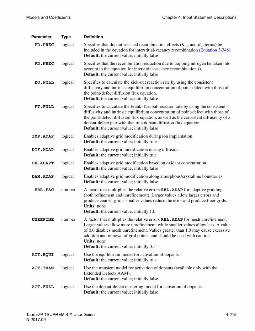
Models and Coefficients Chapter 4: Input Statement Descriptions

PD.PREC logical Specifies that dopant-assisted recombination effects (Kmv and Kni terms) be included in the equation for interstitial-vacancy recombination (Equation 3-348).Default: the current value; initially false

PD.NREC logical Specifies that the recombination reduction due to trapping nitrogen be taken into account in the equation for interstitial-vacancy recombination ().Default: the current value; initially false

KO.FULL logical Specifies to calculate the kick-out reaction rate by using the consistent diffusivity and intrinsic equilibrium concentration of point-defect with those of the point-defect diffusion flux equation.Default: the current value; initially false

FT.FULL logical Specifies to calculate the Frank-Turnbull reaction rate by using the consistent diffusivity and intrinsic equilibrium concentration of point-defect with those of the point-defect diffusion flux equation, as well as the consistent diffusivity of a dopant-defect pair with that of a dopant diffusion flux equation.Default: the current value; initially false

IMP.ADAP logical Enables adaptive grid modification during ion implantation.Default: the current value; initially true

DIF.ADAP logical Enables adaptive grid modification during diffusion.Default: the current value; initially true

OX.ADAPT logical Enables adaptive grid modification based on oxidant concentration.Default: the current value; initially false

DAM.ADAP logical Enables adaptive grid modification along amorphous/crystalline boundaries.Default: the current value; initially false

ERR.FAC number A factor that multiplies the relative errors REL.ADAP for adaptive gridding (both refinement and unrefinement). Larger values allow larger errors and produce coarser grids; smaller values reduce the error and produce finer grids.Units: noneDefault: the current value; initially 1.0

UNREFINE number A factor that multiplies the relative errors REL.ADAP for mesh unrefinement. Larger values allow more unrefinement, while smaller values allow less. A value of 0.0 disables mesh unrefinement. Values greater than 1.0 may cause excessive addition and removal of grid points, and should be used with caution.Units: noneDefault: the current value; initially 0.1

ACT.EQUI logical Use the equilibrium model for activation of dopants.Default: the current value; initially true

ACT.TRAN logical Use the transient model for activation of dopants (available only with the Extended Defects AAM).Default: the current value; initially false

ACT.FULL logical Use the dopant-defect clustering model for activation of dopants.Default: the current value; initially false

Parameter Type Definition

Taurus™ TSUPREM-4™ User Guide 4-215N-2017.09

Chapter 4: Input Statement Descriptions Models and Coefficients

DDC.FULL logical Use the full dopant-defect clustering model for activation of dopants.Default: the current value; initially false

INIT.TIM number The size of the initial time step. Units: minutes Default: the current value; initially 0.002

TIME.DEL number The virtual delta time duration for abrupt temperature ramp. Units: minutes Default: the current value; initially 1.67x10-26

M.AUTO logical Automatically tune the numerical method on the fly.Default: the current value; initially true

MAX.ALLO number Defines the maximum amount of memory to be allocated for the solution matrix when M.AUTO is used. A value of zero implies no limit.Units: bytes Default: 0.0

CG logical Use a conjugate residual method to solve the system of blocks. Default: the current value; initially true

GCR logical Use a modified conjugate residual method to solve the system of blocks. Default: the current value; initially false

SPLU logical Use a sparse direct method with pivoting to solve the system of blocks. Default: the current value; initially false

BACK number The number of back vectors to be used in the CG outer iteration. The maximum value is 48. More back vectors should give faster convergence but require more memory. Units: none Default: the current value; initially 18

BLK.ITLI number The maximum number of block iterations allowed. The block iteration terminates after this number of iterations, whether convergence is obtained or not. Units: none Default: the current value; initially 20

PRECOND number Selects the preconditioner to be used for CG and GCR methods. PRECOND=1 selects the preconditioner used in previous releases while PRECOND=2 selects a new preconditioner. PRECOND=2 is faster for difficult problems, including most cases using PD.5STR (that is, NSTREAM=5); PRECOND=1 is faster for most other problems. PRECOND=2 may be faster for 1D (or quasi 1D) problems. PRECOND=2 (with appropriate values of MF.F.LEV and MF.P.LEV) is faster than SPLU in most cases.Units: none Default: the current value; initially 1

MIN.FILL logical Use a minimum fill reordering for the matrices, to increase solution speed.Default: the current value; initially true

Parameter Type Definition

4-216 Taurus™ TSUPREM-4™ User GuideN-2017.09

Models and Coefficients Chapter 4: Input Statement Descriptions

MIN.FREQ number Controls how much the solution matrix may increase before a new minimum fill reordering is done. A value of zero forces a minimum fill reordering whenever the matrix structure changes. Units: noneDefault: the current value; initially 1.1

MF.METH number Selects the algorithm to use for minimum fill reordering. A value of 0 selects the algorithm used prior to Version 6.6, while a value of 1 selects the algorithm prior to Version 2006.06. A value of 2 selects a minimum fill reordering method that reduces the number of low-order fill terms, which usually produces faster solutions than 0 or 1 methods.Units: none Default: the current value; initially 1

MF.DIST number The maximum distance between nodes, for which fill terms are included when FULL fill is specified. Smaller values decrease the time and memory required for matrix decomposition, but may increase the number of iterations required for solution; very large values (larger than the size of the structure) retain all fill terms, as in versions prior to 6.6.Units: micronsDefault: the current value; initially 0.5

MF.P.LEV number Limits the level of fill terms used for METHOD PART solutions (PRECOND=1) or for coupling between different solutions (PRECOND=2). Values are the same as for MF.F.LEV. The default value of 2 produces the same result for PRECOND=1 as in previous versions of the program. On difficult problems with PRECOND=2, the solution may be considerably faster with a value of 1 or 3 for MP.P.LEV. A value of zero specifies that the level of fill terms is not limited. MF.P.LEV is only used when MF.DIST is nonzero. If MF.P.LEV > MF.F.LEV, the value of MF.F.LEV is used instead.Units: noneDefault: the current value; initially 2

MF.F.LEV number Limits the level of fill terms used for METHOD FULL solutions (PRECOND=1) or for coupling between nodes for a given solution (PRECOND=2). A value of 1 uses no fill terms; a value of 2 uses fill terms produced by original matrix entries; a value of 3 uses fill terms arising from level 2 fill terms; and so on. Larger values require more solution time per CG or GCR iteration but may reduce the number of iterations required. A value of zero specifies that the level of fill terms is not limited. MF.F.LEV is only used when MF.DIST is nonzero.Units: noneDefault: the current value; initially 5

IMPURITY character A list of one or more impurities (separated by spaces or commas) to which the remaining parameters apply. (The list must be enclosed in quotes if it contains spaces.)Default: none Synonym: IMP

Parameter Type Definition

Taurus™ TSUPREM-4™ User Guide 4-217N-2017.09

Chapter 4: Input Statement Descriptions Models and Coefficients

VACANCY logical The remaining parameters apply to the solution for vacancies. Default: false Synonym: VACANCIE

INTERSTI logical The remaining parameters apply to the solution for interstitials. Default: false

ANTIMONY logical The remaining parameters apply to the solution for antimony. Default: false Synonym: SB

ARSENIC logical The remaining parameters apply to the solution for arsenic. Default: false Synonym: AS

BORON logical The remaining parameters apply to the solution for boron. Default: false Synonym: B

PHOSPHOR logical The remaining parameters apply to the solution for phosphorus. Default: false Synonym: P

OXIDANT logical The remaining parameters apply to the solution for oxidant. Default: false Synonym: OXYGEN

TRAP logical The remaining parameters apply to the solution for interstitial traps. Default: false

FULL logical Use all terms produced in factorization of the block matrices for the selected solution variables. Default: the current value; initially true for VACANCY and INTERSTI blocks, false for others

PART logical Use only nearest neighbor fill terms produced in factorization of the block matrices for the selected solution variables. Default: the current value; initially true for mobile species except VACANCY and INTERSTI, and false for all others

NONE logical Do not use fill terms produced during factorization of the block matrices for the selected solution variables. Default: the current value; initially true for immobile species, false for others

SYMMETRY logical Treat the block matrix equations for the selected solution variables as if they were symmetric. Default: the current value; initially false for all blocks Synonym: SYMMETRI

TIME.STE logical The matrices for the selected solution variables are refactored at each time step. Default: the current value; initially true for all blocks

ERROR logical The matrices for the selected solution variables are refactored whenever the error in the block is decreasing. Default: the current value; initially false for all blocks

Parameter Type Definition

4-218 Taurus™ TSUPREM-4™ User GuideN-2017.09

Models and Coefficients Chapter 4: Input Statement Descriptions

NEWTON logical The matrices for the selected solution variables are refactored at each Newton step. Default: the current value; initially false for all blocks

REL.ERR number The relative error tolerance for solution of the impurity blocks for the selected solution variables. Units: none Default: the current value; initially 0.01 for all blocks

ABS.ERR number The absolute error tolerance for solution of the impurity blocks for the selected solution variables. Units: The units of the solution variable. Default: the current value; initially 1e5 for VACANCY and INTERSTI blocks, 1e9 for others

TEMP.MIN number The minimum temperature at which the equation is to be solvedUnits: oCDefault: the current value; initially -273.16 oC for PSI and stress solutions, 450oC for others

MATERIAL character A list of one or more materials (separated by spaces or commas), in which the specified values of REL.ADAP, ABS.ADAP, and MIN.SPAC apply. (The list must be enclosed in quotes if it contains spaces.)Default: none

SILICON logical The specified values of REL.ADAP, ABS.ADAP, and MIN.SPAC apply in single-crystal silicon.Default: false

POLYSILI logical The specified values of REL.ADAP, ABS.ADAP, and MIN.SPAC apply in polysilicon.Default: false

OXIDE logical The specified values of REL.ADAP, ABS.ADAP, and MIN.SPAC apply in oxide.Default: false

OXYNITRI logical The specified values of REL.ADAP, ABS.ADAP, and MIN.SPAC apply in oxynitride.Default: false

NITRIDE logical The specified values of REL.ADAP, ABS.ADAP, and MIN.SPAC apply in nitride.Default: false

ALUMINUM logical The specified values of REL.ADAP, ABS.ADAP, and MIN.SPAC apply in aluminum.Default: false

PHOTORES logical The specified values of REL.ADAP, ABS.ADAP, and MIN.SPAC apply in photoresist.Default: false

Parameter Type Definition

Taurus™ TSUPREM-4™ User Guide 4-219N-2017.09

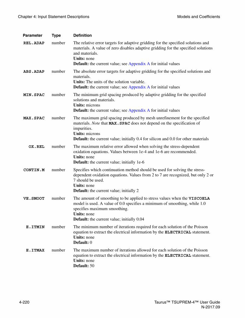
Chapter 4: Input Statement Descriptions Models and Coefficients

REL.ADAP number The relative error targets for adaptive gridding for the specified solutions and materials. A value of zero disables adaptive gridding for the specified solutions and materials.Units: noneDefault: the current value; see Appendix A for initial values

ABS.ADAP number The absolute error targets for adaptive gridding for the specified solutions and materials.Units: The units of the solution variable.Default: the current value; see Appendix A for initial values

MIN.SPAC number The minimum grid spacing produced by adaptive gridding for the specified solutions and materials.Units: micronsDefault: the current value; see Appendix A for initial values

MAX.SPAC number The maximum grid spacing produced by mesh unrefinement for the specified materials. Note that MAX.SPAC does not depend on the specification of impurities.Units: micronsDefault: the current value; initially 0.4 for silicon and 0.0 for other materials

OX.REL number The maximum relative error allowed when solving the stress-dependent oxidation equations. Values between 1e-4 and 1e-6 are recommended.Units: none Default: the current value; initially 1e-6

CONTIN.M number Specifies which continuation method should be used for solving the stress-dependent oxidation equations. Values from 2 to 7 are recognized, but only 2 or 7 should be used.Units: none Default: the current value; initially 2

VE.SMOOT number The amount of smoothing to be applied to stress values when the VISCOELA model is used. A value of 0.0 specifies a minimum of smoothing, while 1.0 specifies maximum smoothing.Units: noneDefault: the current value; initially 0.04

E.ITMIN number The minimum number of iterations required for each solution of the Poisson equation to extract the electrical information by the ELECTRICAL statement.Units: noneDefault: 0

E.ITMAX number The maximum number of iterations allowed for each solution of the Poisson equation to extract the electrical information by the ELECTRICAL statement.Units: noneDefault: 50

Parameter Type Definition

4-220 Taurus™ TSUPREM-4™ User GuideN-2017.09

Models and Coefficients Chapter 4: Input Statement Descriptions

E.RELERR number The allowed relative error used to test for convergence during the iterative numerical solution of the Poisson equation. This value determines the maximum relative change between successive approximations to the solution during iteration. This value is used to extract the electrical information by the ELECTRICAL statement.Units: noneDefault: 0.0001

E.RVCAP number The ratio of AC disturbance to DC incremental voltage to extract the capacitance by the ELECTRICAL statement.Units: noneDefault: 0.2

E.AVCAP number Disturbance voltage to extract the capacitance by the ELECTRICAL statement.Units: voltagesDefault: 0.025

E.USEAVC number Specifies that E.AVCAP is to be used for capacitance extraction in the ELECTRICAL statement. If false, E.RVCAP is used.Default: false

E.REGRID logical Specifies that the automatic regridding is to be performed before solving the Poisson equation.Default: true

E.TSURF number The thickness of surface region to be regridded by specifying E.REGRID.Units: umDefault: 0.01

E.DSURF number The first grid space after regridding by specifying E.REGRID.Units: umDefault: 0.0002

E.RSURF number The ratio between sequent grid spaces after regridding by specifying E.REGRID.Units: noneDefault: 1.2

MOB.TABL logical Specifies that the mobility tables are used to determine electron and hole mobilities.Default: true

MOB.AROR logical Specifies that the analytic mobility model based on the work of Arora, et al., is used to determine electron and hole mobilities.Default: false

MOB.CAUG logical Specifies that the analytic mobility model based on the work of Caughey, et al., is used to determine electron and hole mobilities.Default: false

ITRAP logical Use the interface trap model for segregation flux.Default: false

Parameter Type Definition

Taurus™ TSUPREM-4™ User Guide 4-221N-2017.09

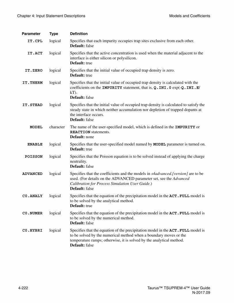
Chapter 4: Input Statement Descriptions Models and Coefficients

IT.CPL logical Specifies that each impurity occupies trap sites exclusive from each other.Default: false

IT.ACT logical Specifies that the active concentration is used when the material adjacent to the interface is either silicon or polysilicon.Default: true

IT.ZERO logical Specifies that the initial value of occupied trap density is zero.Default: true

IT.THERM logical Specifies that the initial value of occupied trap density is calculated with the coefficients on the IMPURITY statement, that is, Q.INI.0 exp(-Q.INI.E/kT).Default: false

IT.STEAD logical Specifies that the initial value of occupied trap density is calculated to satisfy the steady state in which neither accumulation nor depletion of trapped dopants at the interface occurs.Default: false

MODEL character The name of the user-specified model, which is defined in the IMPURITY or REACTION statements.Default: none

ENABLE logical Specifies that the user-specified model named by MODEL parameter is turned on.Default: true

POISSON logical Specifies that the Poisson equation is to be solved instead of applying the charge neutrality.Default: false

ADVANCED logical Specifies that the coefficients and the models in s4advanced.[version] are to be used. (For details on the ADVANCED parameter set, see the Advanced Calibration for Process Simulation User Guide.)Default: false

C0.ANALY logical Specifies that the equation of the precipitation model in the ACT.FULL model is to be solved by the analytical method.Default: true

C0.NUMER logical Specifies that the equation of the precipitation model in the ACT.FULL model is to be solved by the numerical method.Default: false

C0.HYBRI logical Specifies that the equation of the precipitation model in the ACT.FULL model is to be solved by the numerical method when a boundary moves or the temperature ramps; otherwise, it is solved by the analytical method.Default: false

Parameter Type Definition

4-222 Taurus™ TSUPREM-4™ User GuideN-2017.09

Models and Coefficients Chapter 4: Input Statement Descriptions

C0.TRAN logical Specifies to update the C0 solution during temperature ramp so that the active concentration must be always bigger than ACT.NI times the intrinsic carrier concentration, which is compatible with the ACT.TRAN. When C0.TRAN is turned off, the ACT.NI limited activation is applied only at the C0 initialization following an implant. Applied only to the ACT.FULL model with positive ACT.NI value.Default: false

EQACT.A logical Specifies to force the initial active concentration not to exceed its equilibrium concentration. Applied only to the ACT.FULL model with positive ACT.NI value.Default: false

II.TOL.F number The factor to control the tolerance for taking account of the contribution from the lateral distribution of neighbor as-implant profile. It may not be negative and not exceed 1.0.Units: noneDefault: 0.1

II.IF.DY number The thickness of the transition region between profiles at material interfaces for calculation of lateral scattering.Units: micronsDefault: the current value; initially 1e-4

II.GE.EF logical Apply the Ge-Dependent Reshaping Implant Model. Applied only for Taurus Analytic Implant Model.Default: false

II.MOLEC logical Add fluorine atoms for BF2 implants.Default: false

TABLE character Sets the default value of the file name suffix for the implant tables which contain the desired implant data in the format of ion_in_material_suffix. This parameter changes the default suffix for all materials. The DATA.SUF parameter of the IMPLANT command can be used to change the suffix for a single process step. Applies only to the Taurus Analytic Implant Model.Default: STANDARD

DAM.TABL character Sets the default value of the file name suffix for the implant tables which contain the desired implant damage data in the format of ion_damage_in_material_suffix. This parameter changes the default suffix for all materials. The DAM.SUF parameter of the IMPLANT command can be used to change the suffix for a single process step. Applies only to the Taurus Analytic Implant Model.Default: STANDARD

BACKSCAT logical Enables or disables backscattering by default for Taurus implants. The value of this parameter is overridden by the value of the BACKSCAT parameter of the IMPLANT command (if specified). Applies only to the Taurus Analytic Implant Model.Default: true

Parameter Type Definition

Taurus™ TSUPREM-4™ User Guide 4-223N-2017.09

Chapter 4: Input Statement Descriptions Models and Coefficients

RANGE.SH logical Selects the default approach for shifting the projected ranges in multilayer targets. The value of this parameter is overridden by the value of the RANGE.SH parameter of the IMPLANT command (if specified). Applies only to the Taurus Analytic Implant Model.Default: true

DUAL.LAT logical Forces to integrate the lateral distributions of both amorphous and channeled profiles. Applies only to the Taurus Analytic Implant Model.Default: false

D.SCALE number The default scale factor applied to the Frenkel pair component of the damage profile. Applies only to the Taurus Analytic Implant Model. Units: noneDefault: 1.0

TRAJ.REP logical Global switch for trajectory replication.Default: false

X.INTERV number The length of each segment of the replication subwindow.Unit: micronsDefault: 0.02

TRAJ.SPL logical Global switch for trajectory splitting.Default: false

DEPTH.SP logical Depth distribution: Specify the trajectory splitting model which uses the depth distribution of the dopant as splitting criterion.Default: true

COLL.DEN logical Specifies the trajectory splitting model which uses the collision density as splitting criterion.Default: false

TRAJ.DEN logical Specifies the trajectory splitting model which uses the trajectory density as splitting criterion.Default: false

MULT.ROT number The number of the rotations by the rotational angle 360/MULT.ROT degrees for the rotating implant.Units: noneDefault: 1Synonym: MULTROT

MULT.ETC number specifies that an isotropic etch step is to be performed by MULT.ETC-steps instead of one step.Units: noneDefault: 1Synonym: MULTETCH

PRINT logical Print the current model setting.Default: false

Parameter Type Definition

4-224 Taurus™ TSUPREM-4™ User GuideN-2017.09

Models and Coefficients Chapter 4: Input Statement Descriptions

Description The METHOD statement selects the models to be used for local oxidation and point defect kinetics, and specifies numerical algorithms to be used for solving the simulation equations. Most users need be concerned only with the parameters for selecting the local oxidation model and the point defect models. Appropriate defaults for all values are given in the s4init file.

Oxidation Models The oxidation model is selected by specifying one of the ERFC, ERF1, ERF2, ERFG, VERTICAL, COMPRESS, VISCOELA, or VISCOUS parameters. Parameters for the oxidation models are given on the AMBIENT statement. See AMBIENT, p. 4-236 for an overview of the models and their parameters, and see Chapter 3, Oxidation, p. 3-99, for a complete description.

Grid Spacing inGrowing Oxide

The DY.OXIDE, DY.EXACT, DY.LOCAL, and GRID.OXI parameters control the addition of grid to growing oxide layers, as described in Chapter 3, Addition of Nodes in a Growing Layer, p. 3-9. DY.OXIDE is the preferred parameter for controlling the grid spacing in growing oxides; the GRID.OXI parameter is considered obsolete, and is provided only for compatibility with old input files.

Note:The default value for GRID.OXI is set every time a METHOD statement is processed; for GRID.OXI to have an effect, it must be specified on the last METHOD statement before an oxidation step.

Rigid VersusViscous

Substrate

The SKIP.SIL parameter determines whether silicon regions are treated as a rigid substrate (SKIP.SIL true) or a viscous or viscoelastic material (SKIP.SIL false) during oxidation with the VISCOUS or VISCOELA model. Simulation of oxidation is much faster when SKIP.SIL is true, but stresses in the silicon are only calculated when SKIP.SIL is false.

To obtain the stresses in the silicon at the end of an oxidation step using the VISCOUS model, SKIP.SIL can be set to false for a very short oxidation step, and then reset to true:

$ Assume SKIP.SIL is true to start withDIFFUSE TIME=60 TEMPERAT=1000 WETO2

$ Very short step with skip.sil false$ for stress calculationMETHOD ^SKIP.SILDIFFUSE TIME=1E-6 TEMPERAT=1000 WETO2

$ Reset skip.sil to true for next timeMETHOD SKIP.SIL

When the VISCOELA model is used, SKIP.SIL must be set to false for the entire simulation if stresses in the substrate are needed.

Another case in which SKIP.SIL should be set false is when simulating mesa structures, where the lifting of the edge of a silicon mesa may occur. Note that the SKIP.SIL parameter only affects oxidation with the VISCOUS and VISCOELA

Taurus™ TSUPREM-4™ User Guide 4-225N-2017.09

Chapter 4: Input Statement Descriptions Models and Coefficients

models; silicon is always treated as a rigid substrate when the other oxidation models are used.

Point DefectModeling

The level of point defect modeling is set by the NSTREAMS parameter, and the details of the model are selected by the PAIR.GRA, PAIR.SAT, PAIR.REC, PD.PFLUX, PD.PTIME, and PD.PREC parameters. The PD.FERMI, PD.TRANS, and PD.FULL parameters provide convenient ways of setting the most useful combinations of NSTREAMS, PAIR.GRA, PAIR.SAT, PAIR.REC, PD.PFLUX, PD.PTIME, and PD.PREC.

PD.FERMI Model The simplest (and fastest) model is PD.FERMI, in which the point defect concentrations depend only on the Fermi level in the silicon. (The actual point defect concentrations are not calculated, the effects of the Fermi level being included implicitly in the models of impurity diffusion.) The PD.FERMI model does not model oxidation-enhanced diffusion, high concentration, or implant damage effects. This model should be used when speed of the simulation is more important than accuracy, or when it is known that the features of the more complicated models are not needed.

PD.TRANS Model The PD.TRANS parameter causes a full, transient simulation of the 2D point defect distributions to be performed. The model includes the generation of point defects at interfaces, the diffusion of point defects into the substrate, and recombination at interfaces and in bulk silicon. The PD.TRANS model simulates oxidation-enhanced diffusion, but does not model high concentration effects (for example, phosphorus kink and tail). It is less accurate than the PD.FULL model when simulating implant damage effects. The parameters for the point defect models are specified on the INTERSTITIAL and VACANCY statements. This model is recommended for routine simulations.

PD.FULL Model The PD.FULL model includes all the effects of the PD.TRANS model plus the effects of dopant diffusion on the point defect concentration. It also includes pair saturation and dopant-assisted recombination effects. The PD.FULL model simulates oxidation-enhanced diffusion and high concentration (for example, phosphorus kink and tail), and implant damage effects (when used with the DAMAGE parameter on the IMPLANT statement). This model is recommended when it is known that high-concentration or implant damage effects are important.

PD.5STR Model Turning on PD.5STR or setting NSTREAM to 5 causes the transient simulation of dopant-defect pairing as well as all the effects of the PD.FULL model. This model is the most accurate diffusion model available, but requires the most computer time. This model is recommended only when the maximum available accuracy is needed, or when it is known that very low temperature or very short time process following implants is important. If the solution values of a dopant-defect pair are all zeros, the pair solution is removed. For example, by default, phosphorus atoms diffuse by pairing only with interstitials so that the values of the

4-226 Taurus™ TSUPREM-4™ User GuideN-2017.09

Models and Coefficients Chapter 4: Input Statement Descriptions

solution vpair_phosphor are all zeros. Then TSUPREM-4 removes the equation for vpair_phosphorus

METHOD PD.5STR

Customizing thePoint Defect

Models

The PD.FERMI, PD.TRANS, and PD.FULL parameters are processed before the other diffusion model specifications, so you can modify these models by simultaneous specification of the PAIR.GRA, PAIR.SAT, PAIR.REC, PD.PFLUX, PD.PTIME, and PD.PREC parameters. For example:

METHOD PD.TRANS PD.PFLUX

selects the basic 3-stream diffusion model, but includes the dopant-defect pair flux terms in the equations for interstitials and vacancies. This combination is useful because it provides a reasonable approximation to high-concentration effects without the computational overhead of the complete PD.FULL model. Similarly, the statement:

METHOD PD.FULL ^PAIR.REC

removes the complicated (but generally insignificant) dopant-assisted recombination factors from the equations for dopant diffusion.

Enable/DisableUser-Specified

Models

The MODEL and ENABLE parameters provides the way to enable or disable the equations specified by users in the IMPURITY or REACTION statements. For example, the below statement designates that all equations named to myModel in the IMPURITY or REACTION statements must be solved:

METHOD MODEL=myModel ENABLE

On the other hand, the below statement disables the equations:

METHOD MODEL=myModel ^ENABLE

Solving thePoisson

Equation

By default, the electron concentration is analytically calculated by assuming local charge neutrality, which is reasonably good assumption for the semiconductor thermal process. However, as the temperature of the thermal process decreases, and as the abruptness of the doping profile near a PN junction increases, the charge neutrality assumption results in the incorrect electric field near the junction. To calculate more accurate electric field, the Poisson equation needs to be numerically solved. Turning on POISSON parameter in the METHOD statement specifies the Poisson equation to be solved.

METHOD POISSON

The solution name of the potential is PSI.

Note:The Poisson equation is solved only for silicon and polysilicon materials.

Taurus™ TSUPREM-4™ User Guide 4-227N-2017.09

Chapter 4: Input Statement Descriptions Models and Coefficients

AdaptiveGridding

The IMP.ADAP, DIF.ADAP, OX.ADAPT, ERR.FAC, and UNREFINE parameters provide high-level control over adaptive gridding. IMP.ADAP enables or disables adaptive mesh refinement during ion implantation, which ensures that the grid is fine enough to resolve the implanted profile.

Note:Adaptive grid only works with the analytical implant models; it is not available when the MC implant model is specified.

DIF.ADAP enables or disables adaptive gridding during diffusion. Adaptive mesh refinement during diffusion ensures that accuracy is not degraded when profiles diffuse into regions where the grid is too coarse. If the value of UNREFINE is greater than zero, mesh unrefinement will be performed to remove mesh points that are no longer needed to ensure an accurate solution.

Note:You may want to disable adaptive gridding during diffusion immediately following a MC implant. Adaptive gridding can be turned back on after any statistical noise from the MC implant has been smoothed by the diffusion process.

OX.ADAPT controls adaptive gridding in oxide based on oxidant concentration. Its use can significantly improve the accuracy of oxide shapes, especially when specifying a coarse starting grid or large value of DY.OXIDE. On the other hand, there are some situations in which OX.ADAPT can produce an unnecessarily large number of grid points. For example, when oxidizing through a poly layer, it may be advisable to disable OX.ADAPT between the time when the oxidation first breaks through the poly and the time when the poly layer has been consumed across its entire width. This avoids adding unnecessary extra nodes in the pad oxide under the poly.

The interstitial distribution is necessarily abrupt near amorphous and crystalline boundary after regrowth because the boundary location is determined by comparing implant damage concentration to the MAX.DAM parameter value.Then the interstitial concentration is reset to the equilibrium value in the regrowth region. Thus, the interstitial dose so Transient Enhanced Diffusion (TED) is sensitive to the mesh density near the boundary region. By switching on DAM.ADAP, the adaptive gridding method based on the phase transition between amorphous and crystalline regions makes denser mesh near the boundary so that it increases simulation accuracy. Unlike the adaptive gridding of other solutions that uses the absolute and relative errors based on the solution values, the adaptive gridding for damage solution is performed on the transformed profile of damage: The ABS.ADAP and REL.ADAP parameter values for damage is associated with the value s of Equations 4-5, not with the damage concentration itself:

Equation 4-5

ERR.FAC controls the level of adaptive gridding by scaling the relative error targets specified by REL.ADAP. Larger values of ERR.FAC allow larger relative

s 1 DAM.GRAD ln D0 MAX.DAMA⁄( )×[ ]tanh+=

4-228 Taurus™ TSUPREM-4™ User GuideN-2017.09

Models and Coefficients Chapter 4: Input Statement Descriptions

errors and produce coarser grids; smaller values of ERR.FAC reduce the relative errors, producing finer grids. UNREFINE controls the level of mesh unrefinement by scaling the relative error used for refinement. A value of 1.0 gives the same error level for refinement and unrefinement, while a value of 0.0 disables unrefinement.

Fine Control Fine control over adaptive gridding is provided with the REL.ADAP, ABS.ADAP, MIN.SPAC, and MAX.SPAC parameters. REL.ADAP and ABS.ADAP specify the relative and absolute error targets for the specified solution variables and materials. MIN.SPAC specifies the minimum grid spacing produced by adaptive refinement, and MAX.SPAC specifies the maximum grid spacing produced by unrefinement. The value of MIN.SPAC should be small enough to resolve implanted and diffused impurity profiles, but if it is made too small, simulation times may become very large, especially during oxidation steps. MAX.SPAC can be set to zero to disable mesh unrefinement in selected materials.

See Adaptive Gridding, p. 4-228 for further information on the use of adaptive gridding.

Initial Time Step The INIT.TIM parameter specifies the initial time step to be used for diffusion steps. The default value is usually adequate, but some speedup can be obtained by specifying a larger value when appropriate. Smaller values may be advisable following an ion implantation with damage, when growing an initial oxide, or when the structure contains sharply peaked impurity distributions.

Internal SolutionMethods

The remaining parameters specify the internal solution methods to be used.

CAUTIONThese values should not be changed except by the experienced user. Some of the remaining parameters may be changed or eliminated in future releases of the program, in which case input files that use these parameters need to be modified.

Time Integration The TRBDF method is used for time integration. The MILNE, HYBRID, and FORMULA parameters are provided for compatibility with old input files, but only the TRBDF method is supported.

A TRBDF integration step consists of a trapezoidal step followed by a backward difference step. A second trapezoidal solution is used to estimate the local truncation error and to determine the size of the next time step.

Note:The parameters governing the matrix solution algorithms should be changed only if there is a demonstrated need for doing so. The use of

Taurus™ TSUPREM-4™ User Guide 4-229N-2017.09

Chapter 4: Input Statement Descriptions Models and Coefficients

inappropriate combinations of values for these parameters may prevent the solution algorithms from converging.

SystemSolutions

The equations for each impurity (and for oxidant) form a block. Each block is solved independently, then the system of blocks is solved by an outer iteration method. The CG parameter selects a conjugate residual method for the outer iteration method. The BACK parameter specifies the maximum number of back vectors to be used in the CG method. The number of outer iterations is limited to BLK.ITLI; the iteration is terminated at this point, whether convergence has been reached or not. The GAUSS method is no longer supported, and may not work in this or future versions of the program.

The advanced direct solver SPLU implements sparse LU decomposition with partial pivoting, optimized toward the process simulation applications. The iterative CG method is still recommended to use by default, unless you experience convergence problems. In which case we suggest to use the direct SPLU solver instead.

Minimum-FillReordering

A minimum-fill reordering is performed to reduce the solution time for the impurity blocks if the MIN.FILL parameter is true. The MIN.FREQ parameter sets a limit on how much the solution matrix may expand before the minimum-fill reordering is repeated. A value of zero forces a reordering whenever the grid structure changes; a value greater than one reduces the time spent reordering equations but increases the time required to solve them. Using MIN.FILL is strongly advised.

The algorithm for minimum-fill reordering is selected by the MF.METH parameter. MF.METH=0 specifies a complex algorithm designed to give optimum results when FULL factorization with a very large value of MF.DIST is used. MF.METH=1 specifies a simpler algorithm that is much faster, and appears to work at least as well as the older algorithm for most cases encountered in TSUPREM-4. MF.DIST specifies the distance between nodes in the structure beyond which fill terms can be ignored when FULL fill is used.

Block Solution The remaining parameters apply to solving the equations for the specified impurity.

Automatic Tunefor OptimalNumerical

Method

The more complicated the simulation problem, the more difficult it is to set the optimal values of the numerical parameters. Furthermore, you must have proficient knowledge of the numerical algorithm, which is beyond normal process engineering. This feature automatically tunes the parameter values on the fly so users do not need to know the numerical algorithm. This feature also improves the simulation speed. When the Boolean parameter M.AUTO is switched on, it automatically tunes the linear solver method to generate the optimal preconditioner, minimum fill reordering, and to control the block iteration limit, that is, CG/GCR/SPLU, PRECOND, MF.METH, MF.DIST, MF.P.LEV, MF.F.LEV, and BLK.ITLI.

4-230 Taurus™ TSUPREM-4™ User GuideN-2017.09

Models and Coefficients Chapter 4: Input Statement Descriptions

Solution Method The LU solution method has been found to be most effective for all impurities, and is much faster than the others for point defects. The SOR, SIP, and ICCG methods are no longer supported, and may not work in this or future versions of the program.

Matrix Structure The FULL, PART, and NONE parameters specify the degree to which fill-in terms are to be included in the matrix solution. PART and NONE produce smaller matrices that are faster to decompose, but which may require more iterations. PART is useful for impurities. Using FULL for point defects is generally fastest, but may generate a large number of floating-point underflow conditions. This can cause a large reduction in speed on computers that use software trapping to process subnormal floating point numbers. On such machines, it is better to use PART for point defects. An appropriate value for MF.DIST can also alleviate this problem. NONE can be used for interstitial traps, and other species that do not diffuse.

SYMMETRY forces the matrix to be treated as symmetric, whether it is or not. The program may fail if this parameter is set true when it should be false.

MatrixRefactoring

The NEWTON, TIME.STE, and ERROR parameters determine how often the matrix is refactored. Using NEWTON gives the fastest convergence, but spends the most time refactoring the matrix; using TIME.STE causes the matrix to be refactored only at the start of each time step. With ERROR, the matrix is refactored as needed. The TIME.STE choice has been found to give the fastest solution for most problems.

DiscontinuousTemperature

Change

To keep track of stress history by turning on the parameter ST.HIST, the step-like discontinuous change of temperature is not allowed. Instead, TSUPREM-4 internally solves the equations by assuming the delta time step TIME.DEL. Too small TIME.DEL value might cause the convergence problem. 1 s ~ 1ns are recommended.

Error Tolerances The relative and absolute error tolerances for solution of the impurity blocks are given by REL.ERR and ABS.ERR, respectively. The relative error tolerance for stress-dependent oxidation solutions with the VISCOUS model is given by OX.REL, which should be between 1e-4 and 1e-6. CONTIN.M selects a continuation method for solving the stress-dependent oxidation equations (VISCOUS model only). Values from 2 to 7 are recognized, but only Methods 2 and 7 should be used. Method 2 is the method used in versions of TSUPREM-4 before Version 5.1; Method 7 is a new method. Method 7 is more likely to converge than Method 2, but when Method 7 does not converge, its results may be worse.

μ

Taurus™ TSUPREM-4™ User Guide 4-231N-2017.09

Chapter 4: Input Statement Descriptions Models and Coefficients

More AccurateDose Integration

From LateralDistribution

When dopants coming from lateral distribution of the neighbors are integrated, the calculation time can be saved by checking whether if the dose to be added is smaller than the certain tolerance so that it can be ignored. The parameter II.TOL.F in the METHOD statement defines the control factor for the tolerance. It may not be negative and not exceed 1.0. The smaller value of II.TOL.F means the smaller tolerance so that the calculation is more accurate, but takes more time. By default, it is set to 0.1 from v.2004.09. Setting II.TOL.F to 1.0 provides the backward compatibility. However, note that the value 1.0 of II.TOL.F can cause the mesh-sensitive unsymmetrical as-implant profile even in the case of symmetrical tilt/rotation implants.

Sensitivity ofImplantedProfiles toNonplanarInterfaces

The implant distributions in the layers at an interface overlap, with a linear transition between the distributions as the interface is crossed. Thus when the horizontal line of integration through a node passes through a material interface, the transition from one distribution to another is made over a distance of II.IF.DY/tan( ), where is the angle of the interface. Since tan( )=dY/dX (dY and dX being the Y and X distances between two points on the interface), the transition occurs over a horizontal distance of II.IF.DY.dX/dY. For a nonplanarity of magnitude dY, the effect in the horizontal direction is spread out by the factor II.IF.DY/dY. The transition region between profiles in different materials is either placed entirely in one of the materials or centered on the interface. If the material of the node matches that of one of the materials at the interface, then the transition region is placed in the other material. This means that for an exactly planar interface, there is no difference in the implanted profile; you still get an ideal discontinuity at the interface. If the interface is at the top or bottom of the structure, the transition region is placed outside the structure. If the material at the node and the materials at the interface are all different, the transition region is centered on the interface.

Examples 1. The following statement specifies that the initial time step should be 0.1 minutes:

METHOD INIT.TIM=0.1 PD.FERMI VERTICAL

The PD.FERMI model is used for the point defects, and the VERTICAL model for the oxide growth.

2. The following statement indicates that the arsenic blocks should be solved to a relative error of 0.001 (0.1%) or an absolute error of 1012/cm3, whichever is greater:

METHOD ARSENIC REL.ERR=0.001 ABS.ERR=1.0e12

θ θ θ

4-232 Taurus™ TSUPREM-4™ User GuideN-2017.09

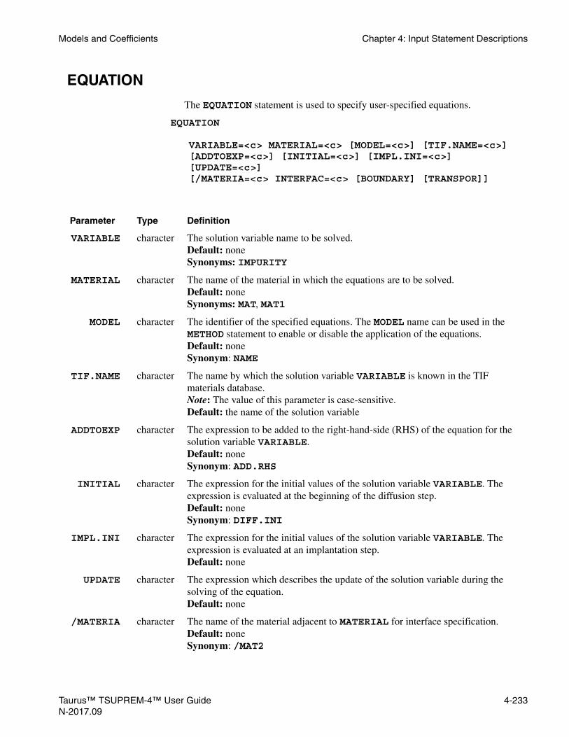
Models and Coefficients Chapter 4: Input Statement Descriptions

EQUATION

The EQUATION statement is used to specify user-specified equations.

EQUATION

VARIABLE=<c> MATERIAL=<c> [MODEL=<c>] [TIF.NAME=<c>][ADDTOEXP=<c>] [INITIAL=<c>] [IMPL.INI=<c>] [UPDATE=<c>][/MATERIA=<c> INTERFAC=<c> [BOUNDARY] [TRANSPOR]]

Parameter Type Definition

VARIABLE character The solution variable name to be solved.Default: noneSynonyms: IMPURITY

MATERIAL character The name of the material in which the equations are to be solved.Default: noneSynonyms: MAT, MAT1

MODEL character The identifier of the specified equations. The MODEL name can be used in the METHOD statement to enable or disable the application of the equations.Default: noneSynonym: NAME

TIF.NAME character The name by which the solution variable VARIABLE is known in the TIF materials database.Note: The value of this parameter is case-sensitive.Default: the name of the solution variable

ADDTOEXP character The expression to be added to the right-hand-side (RHS) of the equation for the solution variable VARIABLE.Default: noneSynonym: ADD.RHS

INITIAL character The expression for the initial values of the solution variable VARIABLE. The expression is evaluated at the beginning of the diffusion step.Default: noneSynonym: DIFF.INI

IMPL.INI character The expression for the initial values of the solution variable VARIABLE. The expression is evaluated at an implantation step.Default: none

UPDATE character The expression which describes the update of the solution variable during the solving of the equation.Default: none

/MATERIA character The name of the material adjacent to MATERIAL for interface specification.Default: noneSynonym: /MAT2

Taurus™ TSUPREM-4™ User Guide 4-233N-2017.09

Chapter 4: Input Statement Descriptions Models and Coefficients

Description The EQUATION statement specifies model equations that have the general form:

at specified boundaries

where X is the quantity to be solved.

TSUPREM-4 assembles the matrices to solve equations by assuming that the time derivative term of X is placed at the left-hand-side (LHS) of the equation and all the other terms at the right-hand-side (RHS). To describe this equation using USEIT, any new terms that appear on the RHS of the equation are specified by the ADDTOEXP (alias ADD.RHS) parameter and the INTERFAC parameter on the EQUATION statement. The INTERFAC parameter is used to define the flux at interfaces. The term Previous_RHS in the above expression represents terms that are already present on the RHS of the equation being modified. The initial condition of the variable X is specified with the INITIAL parameter in the EQUATION statement. The INTERMED statement specifies the intermediate quantities associated with equations.

Since USEIT is designed as a part of TSUPREM-4, you can easily use the physical quantities such as CI.STAR(=I*) and ETA(n/ni) already calculated in the built-in routines. Similarly, you have the choice of using the built-in functions for calculating active and mobile concentrations or defining your own functions with the ACTIVE and MOBILE parameters in the IMPURITY statement.

When a new solution variable is first specified in the EQUATION statement, it is defined automatically. A message is displayed warning that the VARIABLE does not currently exist and is being defined. Alternatively, the solution variable can be defined in the IMPURITY statement with the NEW parameter. The METHOD statement specifies the numerical methods used to solve the equations. The factorization method of block matrices, the absolute, and the relative error tolerances for solutions should be specified.

For additional information, see:

• INTERMEDIATE, p. 4-30 for definitions of INTERMEDIATES used in the expressions of equation.

• METHOD, p. 4-210 for description of numerical methods to solve equations.

INTERFAC character The expression for the flux from /MATERIA to MATERIAL.Default: none

BOUNDARY logical Specifies that the ADDTOEXP expression describes the interface equation.Default: false

TRANSPOR logical Specifies that the INTERFAC flux is taken into account on the nodes in /MATERIA as well.Default: true

Parameter Type Definition

X∂t∂

------ Previous_RHS ADDTOEXP INTERFAC+ +=

4-234 Taurus™ TSUPREM-4™ User GuideN-2017.09

Models and Coefficients Chapter 4: Input Statement Descriptions

• IMPURITY, p. 4-281 for descriptions of calculation methods for active and mobile concentrations.

• Chapter 7, User-Specified Equation Interface for additional details.

Initialization ofSolution

You can define the expression for solution initialization by the INITIAL (alias: DIFF.INI) parameter. The INITIAL expression is performed to initialize a solution at the end of the amorphous regrowth in the first diffusion following an implant or at the beginning of an epitaxy step.

The parameter IMPL.INI defines the expression for the solution initialization at implant. The IMPL.INI expression is evaluated and applied at every implant step.

Figure 4-5 USEIT working diagram

Get

Modify

Implement equations

DIFFI, DIFFV,DIFFUEQACT, ACTIVE

CI.STAR, CV.STARCI.RATIO, CV.RATIOELECTRON, ETAEFIELD

ACTIVE, MOBILE

ADDTOEXP, INTERFACE

Built-inmodelsandfunctions

PDEsolver

USEIT

TSUPREM-4

UsersINITIAL, UPDATE

Taurus™ TSUPREM-4™ User Guide 4-235N-2017.09

Chapter 4: Input Statement Descriptions Models and Coefficients

AMBIENT

The AMBIENT statement is used to specify oxidation coefficients. OXIDE is a valid synonym for the AMBIENT statement.

AMBIENT

[ { DRYO2 | WETO2 | STEAM | N2O | INERT | AMB.1 | AMB.2 | AMB.3 | AMB.4 | AMB.5} [F.O2=<n>] [F.H2O=<n>] [F.N2O=<n>] [F.H2=<n>] [F.N2=<n>]

[F.HCL=<n>][PRESSURE=<n>] [HCL=<n>] ] [ {O2 | H2O | N2O } [ {<111> | <110> | <100> | ORIENTAT=<n> | POLYSILI} [THINOX.0=<n>] [THINOX.E=<n>] [THINOX.L=<n>] [L.LIN.0=<n>] [L.LIN.E=<n>] [H.LIN.0=<n>] [H.LIN.E=<n>]

[N.0=<n>] [N.E=<n>] [N.THIN.0=<n>] [N.THIN.E=<n>] ] [L.PAR.0=<n>] [L.PAR.E=<n>] [H.PAR.0=<n>] [H.PAR.E=<n>] [LIN.BREA=<n>] [PAR.BREA=<n>] [LIN.PDEP=<n>] [PAR.PDEP=<n>] [GAMMA.0=<n>] [GAMMA.E=<n>] [GB.FAC.0=<n>] [GB.FAC.E=<n>] [ { LIN.PCT | PAR.PCT | ( {LIN.CLDE | PAR.CLDE} COLUMN=<n> ) } TABLE=<c> ] [ { MATERIAL=<c> | SILICON | OXIDE | OXYNITRI | NITRIDE | POLYSILI | AMBIENT} [D.0=<n>] [D.E=<n>] [VC=<c>]

[MODEL=<c>] [D.FACTOR=<c>] [R.FACTOR=<c>] [HENRY.CO=<n>] [THETA=<n>] [ { /MATERIA=<c> | /SILICON | /OXIDE | /OXYNITR | /NITRIDE | /POLYSIL | /AMBIENT } [SEG.0=<n>] [SEG.E=<n>] [TRANS.0=<n>] [TRANS.E=<n>] [ALPHA=<n>]

[N.G.0=<n>] [N.G.E=<n>] [N.GPOW.0=<n>] [N.GPOW.E=<n>][N.V.0=<n>] [N.V.E=<n>]

] ] ] [STRESS.D] [ST.R.ANI] [VR=<c>] [VT=<c>] [VD=<c>] [VDLIM=<n>]

[VR100=<c>] [VR110=<c>] [VR111=<c>][VT100=<c>] [VT110=<c>] [VT111=<c>]

[INITIAL=<n>] [SPREAD=<n>] [MASK.EDG=<n>] [ERF.Q=<n>] [ERF.DELT=<n>] [ERF.LBB=<c>] [ERF.H=<c>] [NIT.THIC=<n>]

[CLEAR][TEMPERAT=<c>]

[CM.SEC]

4-236 Taurus™ TSUPREM-4™ User GuideN-2017.09

Models and Coefficients Chapter 4: Input Statement Descriptions

Parameter Type Definition

DRYO2 logical Specifies that the pressure, chlorine percentage, and flows of oxidizing and non-oxidizing species are associated with the dry oxygen ambient.Default: false

WETO2 logical Specifies that the pressure, chlorine percentage, and flows of oxidizing and non-oxidizing species are associated with the wet oxygen ambient.Default: false

STEAM logical Specifies that the pressure, chlorine percentage, and flows of oxidizing and non-oxidizing species are associated with the steam ambient.Default: false

N2O logical Specifies that the pressure, chlorine percentage, and flows of oxidizing and non-oxidizing species are associated with the N2O oxygen ambient.Default: false

INERT logical Specifies that the pressure, chlorine percentage, and flows of oxidizing and non-oxidizing species are associated with the inert ambient.Default: false Synonyms: NEUTRAL, NITROGEN

AMB.1 logical Specifies that the pressure, chlorine percentage, and flows of oxidizing and non-oxidizing species are associated with ambient number 1. Ambient number 1 is defined by the user.Default: false

AMB.2 logical Specifies that the pressure, chlorine percentage, and flows of oxidizing and non-oxidizing species are associated with ambient number 2. Ambient number 2 is defined by the user.Default: false

AMB.3 logical Specifies that the pressure, chlorine percentage, and flows of oxidizing and non-oxidizing species are associated with ambient number 3. Ambient number 3 is defined by the user.Default: false

AMB.4 logical Specifies that the pressure, chlorine percentage, and flows of oxidizing and non-oxidizing species are associated with ambient number 4. Ambient number 4 is defined by the user.Default: false

AMB.5 logical Specifies that the pressure, chlorine percentage, and flows of oxidizing and non-oxidizing species are associated with ambient number 5. Ambient number 5 is defined by the user.Default: false

F.O2 number The flow of O2 associated with the specified ambient. If H2 is also present, the O2 and H2 are assumed to react completely to form H2O. The flows of O2 and H2 are reduced, and the flow of H2O is increased.Units: none Default: 0.0

Taurus™ TSUPREM-4™ User Guide 4-237N-2017.09

Chapter 4: Input Statement Descriptions Models and Coefficients

F.H2O number The flow of H2O associated with the specified ambient. If O2 and H2 are also present, the O2 and H2 are assumed to react completely to form H2O. The flows of O2 and H2 are reduced, and the flow of H2O is increased.Units: none Default: 0.0

F.N2O number The flow of N2O associated with the specified ambient. If H2O or O2 are also present, the flow of N2O gas is assumed to be N2.Units: none Default: 0.0

F.H2 number The flow of H2 associated with the specified ambient. If O2 is also present, the O2 and H2 are assumed to react completely to form H2O. The flows of O2 and H2 are reduced, and the flow of H2O is increased.Units: none Default: 0.0

F.N2 number The flow of N2 (or other inert gasses) associated with the specified ambient.Units: none Default: 0.0

F.HCL number The flow of chlorine associated with the specified ambient.Units: none Default: 0.0

PRESSURE number The default value of total gas pressure for the specified ambient.Units: atmospheres Default: the current value for this ambient; initially 1.0

HCL number The default percentage of chlorine present for the specified ambient.Units: percent Default: calculated from F.HCL

O2 logical Specifies that the oxidation coefficients are associated with the O2 oxidizing species.Default: false

H2O logical Specifies that the oxidation coefficients are associated with the H2O oxidizing species. Default: false

<111> logical Specifies that linear and thin oxide growth rate coefficients apply to <111> orientation silicon.Default: false

<110> logical Specifies that linear and thin oxide growth rate coefficients apply to <110> orientation silicon.Default: false

<100> logical Specifies that linear and thin oxide growth rate coefficients apply to <100> orientation silicon.Default: false

Parameter Type Definition

4-238 Taurus™ TSUPREM-4™ User GuideN-2017.09

Models and Coefficients Chapter 4: Input Statement Descriptions

ORIENTAT number Specifies that linear and thin oxide growth rate coefficients apply to silicon of the specified orientation. Allowed values are 100, 110, and 111.Units: none Default: 100

POLYSILI logical The specified coefficients apply to polysilicon, or the interface between polysilicon and some other material.Default: false

THINOX.0 number The pre-exponential constant in the expression for the thin oxide growth rate parameter.Units: microns/min or cm/s Default: current value for this orientation and oxidant

THINOX.E number The activation energy in the expression for the thin oxide growth rate parameter.Units: electron volts Default: current value for this orientation and oxidant

THINOX.L number The characteristic length in the expression for the thin oxide growth rate parameter.Units: microns Default: current value for this orientation and oxidant

L.LIN.0 number The pre-exponential constant in the expression for the linear oxidation rate for temperatures below the temperature breakpoint set by LIN.BREA.Units: microns/min or cm/s Default: current value for this orientation and oxidant Synonym: LIN.L.0

L.LIN.E number The activation energy in the expression for the linear oxidation rate for temperatures below the temperature breakpoint set by LIN.BREA.Units: electron volts Default: current value for this orientation and oxidant Synonym: LIN.L.E

H.LIN.0 number The pre-exponential constant in the expression for the linear oxidation rate for temperatures above the temperature breakpoint set by LIN.BREA.Units: microns/min or cm/s Default: current value for this orientation and oxidant Synonym: LIN.H.0

H.LIN.E number The activation energy in the expression for the linear oxidation rate for temperatures above the temperature breakpoint set by LIN.BREA.Units: electron volts Default: current value for this orientation and oxidant Synonym: LIN.H.E

N.0 number The pre-exponential constant in the expression for the maximum trap density in the N2O linear oxidation rate.

Units: cm-2

Default: current value for this orientation

Parameter Type Definition

Taurus™ TSUPREM-4™ User Guide 4-239N-2017.09

Chapter 4: Input Statement Descriptions Models and Coefficients

N.E number The activation energy in the expression for the maximum trap density in the N2O linear oxidation rateUnits: electron volts Default: current value for this orientation

N.THIN.0 number The pre-exponential constant in the expression for the maximum trap density in the N2O thin oxidation rate.

Units: cm-2

Default: current value for this orientation

N.THIN.E number The activation energy in the expression for the maximum trap density in the N2O thin oxidation rate.Units: electron volts Default: current value for this orientation

L.PAR.0 number The pre-exponential constant in the expression for the parabolic oxidation rate for temperatures below the temperature breakpoint set by PAR.BREA.

Units: microns2/min or cm2/s Default: current value for this oxidant Synonym: PAR.L.0

L.PAR.E number The activation energy in the expression for the parabolic oxidation rate for temperatures below the temperature breakpoint set by PAR.BREA.Units: electron volts Default: current value for this oxidant Synonym: PAR.L.E

H.PAR.0 number The pre-exponential constant in the expression for the parabolic oxidation rate for temperatures above the temperature breakpoint set by PAR.BREA.

Units: microns2/min or cm2/s Default: current value for this oxidant Synonym: PAR.H.0

H.PAR.E number The activation energy in the expression for the parabolic oxidation rate for temperatures above the temperature breakpoint set by PAR.BREA.Units: electron volts Default: current value for this oxidant Synonym: PAR.H.E

LIN.BREA number The temperature breakpoint at which the temperature dependence of the linear oxidation rate changes.Units: degrees Celsius Default: current value for this oxidant Synonym: L.BREAK

PAR.BREA number The temperature breakpoint at which the temperature dependence of the parabolic oxidation rate changes.Units: degrees Celsius Default: current value for this oxidant Synonym: P.BREAK

Parameter Type Definition

4-240 Taurus™ TSUPREM-4™ User GuideN-2017.09

Models and Coefficients Chapter 4: Input Statement Descriptions

LIN.PDEP number The exponent of the pressure in the expression for the linear oxidation rate.Units: none Default: current value for this oxidant Synonym: L.PDEP

PAR.PDEP number The exponent of the pressure in the expression for the parabolic oxidation rate.Units: none Default: current value for this oxidant Synonym: P.PDEP

GAMMA.0 number The pre-exponential constant in the expression for the impurity concentration dependence of the linear oxidation rate.Units: none Default: current value for this oxidant

GAMMA.E number The activation energy in the expression for the impurity concentration dependence of the linear oxidation rate.Units: electron volts Default: current value for this oxidant

GB.FAC.0 number The pre-exponential constant in the expression for the enhancement of the surface reaction rate at grain boundaries.Units: none Default: current value for this oxidant; initially 10 for all ambients

GB.FAC.E number The activation energy in the expression for the enhancement of the surface reaction rate at grain boundaries.Units: electron volts Default: current value for this oxidant; initially 0 for all ambients

LIN.PCT logical Specifies that the TABLE parameter defines chlorine percentages associated with the rows in the table of coefficients modifying the linear oxidation rate in the presence of chlorine.Default: false

PAR.PCT logical Specifies that the TABLE parameter defines chlorine percentages associated with the rows in the table of coefficients modifying the parabolic oxidation rate in the presence of chlorine.Default: false

LIN.CLDE logical Specifies that the TABLE parameter defines entries in a column of the table of coefficients modifying the linear oxidation rate in the presence of chlorine. The column number is specified with the COLUMN parameter, and is associated with the temperature specified by the TEMPERAT parameter.Default: false

PAR.CLDE logical Specifies that the TABLE parameter defines entries in a column of the table of coefficients modifying the parabolic oxidation rate in the presence of chlorine. The column number is specified with the COLUMN parameter, and is associated with the temperature specified by the TEMPERAT parameter.Default: false

Parameter Type Definition

Taurus™ TSUPREM-4™ User Guide 4-241N-2017.09

Chapter 4: Input Statement Descriptions Models and Coefficients

COLUMN number The column number in the tables of coefficients modifying the linear or parabolic oxidation rates. The coefficients defined by the TABLE parameter are stored in this column of a table. The column number is associated with the temperature specified by the TEMPERAT parameter. There can be, at most, 8 columns in a table, and each column corresponds to one temperature.Units: none Default: none

TABLE character This parameter is interpreted as a series of numeric values, separated by spaces or commas. If the LIN.PCT or PAR.PCT parameter is specified, the TABLE parameter defines the chlorine percentages associated with the rows in the table of coefficients modifying the linear or parabolic oxidation rates, respectively. If the LIN.CLDE or PAR.CLDE parameter is specified, the TABLE parameter defines the entries in a column of the table of coefficients modifying the linear or parabolic oxidation rates, respectively. There can be, at most, eight rows in a table, and each row corresponds to one chlorine percentage. At most, 8 values can be defined with this parameter.Units: percent or none Default: none

MATERIAL character The specified coefficients apply to the named material or to the interface between the named material and some other material. Default: none

SILICON logical The specified coefficients apply to silicon, or the interface between silicon and some other material.Default: false

OXIDE logical The specified coefficients to apply to oxide, or the interface between oxide and some other material.Default: true if no other first material is specified

OXYNITRI logical The specified coefficients to apply to oxynitride, or the interface between oxynitride and some other material.Default: false

NITRIDE logical The specified coefficients to apply to nitride, or the interface between nitride and some other material.Default: false

POLYSILI logical The specified coefficients to apply to polysilicon, or the interface between polysilicon and some other material.Default: false

AMBIENT logical The specified coefficients apply to gas, or the interface between gas and some other material.Default: false Synonym: GAS

Parameter Type Definition

4-242 Taurus™ TSUPREM-4™ User GuideN-2017.09

Models and Coefficients Chapter 4: Input Statement Descriptions

D.0 number The pre-exponential constant in the expression for the diffusivity of oxidant in the specified material.

Units: microns2/min or cm2/s Default: current value for this oxidant and material Synonym: DIFF.0

D.E number The activation energy in the expression for the diffusion of oxidant in the specified material.Units: electron volts Default: current value for this oxidant and material Synonym: DIFF.E

VC character A table of activation volumes as a function of temperature for the dependence of material viscosity on shear stress for the specified material and oxidizing species (O2 or H2O). Entries in the table correspond to temperatures given by the TEMPERAT parameter (see text).

Units: Å3 Default: the current value; initially 300

MODEL character The name of the model for user-defined multiplication factors D.FACTOR and R.FACTOR. Only applicable to D.FACTOR and R.FACTOR.Default: none

D.FACTOR character The expression of the multiplication factor to oxidant diffusivity. Only applicable to the VISCOEL model.Units: noneDefault: “1.0”

R.FACTOR character The expression of the multiplication factor to oxidant surface reaction rate. Only applicable to the VISCOEL model.Units: noneDefault: “1.0”

HENRY.CO number The solubility of oxidant in the specified material at one atmosphere.

Units: atoms/cm3/atm Default: current value for this oxidant and material

THETA number The number of oxide molecules per cubic centimeter of oxide.

Units: atoms/cm3 Default: current value

/MATERIA character The specified coefficients to apply to the interface between the other specified material and this named material. Default: none

/SILICON logical The specified coefficients to apply to the interface between the specified material and silicon.Default: True if no other second material is specified.

/OXIDE logical The specified coefficients to apply to the interface between the specified material and oxide.Default: false

Parameter Type Definition

Taurus™ TSUPREM-4™ User Guide 4-243N-2017.09

Chapter 4: Input Statement Descriptions Models and Coefficients

/OXYNITR logical The specified coefficients to apply to the interface between the specified material and oxynitride.Default: false

/NITRIDE logical The specified coefficients to apply to the interface between the specified material and nitride.Default: false

/POLYSIL logical The specified coefficients to apply to the interface between the specified material and polysilicon.Default: false

/AMBIENT logical The specified coefficients to apply to the interface between the specified material and gas.Default: false Synonym: /GAS

SEG.0 number The pre-exponential constant in the expression for segregation of oxidant between the two specified materials.Units: none Default: current value for this oxidant and these materials

SEG.E number The activation energy in the expression for segregation of oxidant between the two specified materials.Units: electron volts Default: current value for this oxidant and these materials

TRANS.0 number The pre-exponential constant in the expression for transport of oxidant between the two specified materials.Units: microns/min or cm/s Default: the current value for this oxidant and these materials Synonym: TRN.0

TRANS.E number The activation energy in the expression for transport of oxidant between the two specified materials.Units: electron volts Default: the current value for this oxidant and these materials Synonym: TRN.E

ALPHA number The volume expansion ratio between the two specified materials. The defaults are 0.44 for silicon/oxide and polysilicon/oxide, and 1.0 for all other combinations.Units: none Default: the current value for these materials

N.G.0 number The pre-exponential constant in the expression for nitrogen generation rate due to N2O oxidation.

Units: cm-3 Default: the current value for these materials

Parameter Type Definition

4-244 Taurus™ TSUPREM-4™ User GuideN-2017.09

Models and Coefficients Chapter 4: Input Statement Descriptions

N.G.E number The activation energy in the expression for nitrogen generation rate due to N2O oxidation. Units: electron voltsDefault: the current value for these materials

N.GPOW.0 number The pre-exponential constant in the expression for the exponent in the normalized boundary velocity.Units: none Default: the current value for these materials

N.GPOW.E number The activation energy in the expression for the exponent in the normalized boundary velocity of N2O oxidation. Units: electron voltsDefault: the current value for these materials

N.V.0 number The pre-exponential constant in the expression for the normalization velocity of N2O oxidation.Units: cm/sDefault: the current value for these materials

N.V.E number The activation energy in the expression for the normalization velocity of N2O oxidation.Units: none Default: the current value for these materials

STRESS.D logical Specifies that the stress-dependent models for oxide viscosity, oxidant diffusivity, and surface reaction rate are to be used. Default: the current value, initially true

ST.R.ANI logical Specifies that the anisotropic stress dependent reaction rate model for oxidation is to be used.Default: the current value, initially false

VR character A table of activation volumes as a function of temperature for the dependence of oxidation rate at the Si/SiO2 interface on normal stress for the specified oxidizing species (O2 or H2O). Entries in the table correspond to temperatures given by the TEMPERAT parameter (see text).

Units: Å3 Default: the current value; initially 15

VR100 character A table of activation volumes for crystal direction 100 as a function of temperature for the dependence of oxidation rate at the Si/SiO2 interface on normal stress for the specified oxidizing species (O2 or H2O). Entries in the table correspond to temperatures given by the TEMPERAT parameter (see text).

Units: Å3 Default: the current value; initially 15

Parameter Type Definition

Taurus™ TSUPREM-4™ User Guide 4-245N-2017.09

Chapter 4: Input Statement Descriptions Models and Coefficients

VR110 character A table of activation volumes for crystal direction 110 as a function of temperature for the dependence of oxidation rate at the Si/SiO2 interface on normal stress for the specified oxidizing species (O2 or H2O). Entries in the table correspond to temperatures given by the TEMPERAT parameter (see text).

Units: Å3 Default: the current value; initially 15

VR111 character A table of activation volumes for crystal direction 111 as a function of temperature for the dependence of oxidation rate at the Si/SiO2 interface on normal stress for the specified oxidizing species (O2 or H2O). Entries in the table correspond to temperatures given by the TEMPERAT parameter (see text).

Units: Å3 Default: the current value; initially 150

VT character A table of activation volumes as a function of temperature for the dependence of oxidation rate at the Si/SiO2 interface on tangential stress for the specified oxidizing species (O2 or H2O). Entries in the table correspond to temperatures given by the TEMPERAT parameter (see text).

Units: Å3 Default: the current value; initially 0.0

VT100 character A table of activation volumes for crystal direction 100 as a function of temperature for the dependence of oxidation rate at the Si/SiO2 interface on tangential stress for the specified oxidizing species (O2 or H2O). Entries in the table correspond to temperatures given by the TEMPERAT parameter (see text).Units: Å3 Default: the current value; initially 0.0

VT110 character A table of activation volumes for crystal direction 110 as a function of temperature for the dependence of oxidation rate at the Si/SiO2 interface on tangential stress for the specified oxidizing species (O2 or H2O). Entries in the table correspond to temperatures given by the TEMPERAT parameter (see text).Units: Å3 Default: the current value; initially 0.0

VT111 character A table of activation volumes for crystal direction 111 as a function of temperature for the dependence of oxidation rate at the Si/SiO2 interface on tangential stress for the specified oxidizing species (O2 or H2O). Entries in the table correspond to temperatures given by the TEMPERAT parameter (see text).Units: Å3 Default: the current value; initially 0.0

VD character A table of activation volumes as a function of temperature for the dependence of oxidant diffusivity in oxide on pressure for the specified oxidizing species (O2 or H2O). Entries in the table correspond to temperatures given by the TEMPERAT parameter (see text).

Units: Å3 Default: the current value; initially 75

Parameter Type Definition

4-246 Taurus™ TSUPREM-4™ User GuideN-2017.09

Models and Coefficients Chapter 4: Input Statement Descriptions

VDLIM number The maximum increase in oxidant diffusivity produced by the VD parameter.Units: none Default: the current value; initially 1.2

INITIAL number The thickness of the existing oxide at the start of oxidation. Exposed silicon surfaces are covered with this thickness of native oxide before oxidation begins.Units: microns Default: the current value; initially 0.002

SPREAD number The ratio of width to height for the bird’s beak, used in the ERFC model of local oxide shape.Units: none Default: the current value; initially 1.0

MASK.EDG number The assumed position of the mask, used by the analytical models for local oxidation. Oxide grows to the right of the mask edge.Units: microns Default: the current value; initially −200

ERF.Q number The q parameter for the ERFG (Guillemot) model.Units: microns Default: the current value; initially 0.05

ERF.DELT number The delta parameter for the ERFG (Guillemot) model.Units: microns Default: the current value; initially 0.04

ERF.LBB character The length of the bird’s beak for the ERFG (Guillemot) model. This is an arithmetic expression involving the variables Fox (the field oxide thickness, in microns), eox (the pad oxide thickness, in microns), Tox (the oxidation temperature, in degrees Kelvin), and en (the nitride thickness, in microns).Units: microns Default: the current value; initially

(8.25e-3*(1580.3-Tox)*(Fox0.67)*(eox0.3)*exp(-((en-0.08)2)/0.06)).

ERF.H character The ratio of the nitride lifting to the field oxide thickness for the ERFG (Guillemot) model. This is an arithmetic expression involving the variables Fox (the field oxide thickness, in microns), eox (the pad oxide thickness, in microns), Tox (the oxidation temperature, in degrees Kelvin), and en (the nitride thickness, in microns).Units: none Default: the current value; initially (402*(0.445-1.75*en)*exp(-Tox/200))

NIT.THIC number The nitride thickness, en used in the equations for ERF.LBB and ERF.H.Units: microns Default: none

TEMPERAT character The temperature associated with the column in the chlorine tables, given by the COLUMN parameter, or a list of temperatures corresponding to the values of the VC, VD, VR, and/or VT parameters.Units: degrees Celsius Default: none

Parameter Type Definition

Taurus™ TSUPREM-4™ User Guide 4-247N-2017.09

Chapter 4: Input Statement Descriptions Models and Coefficients

Description All parameters relating to oxidation are specified on this statement. The necessary parameters are set by AMBIENT statements in the s4init file, but can be changed by you.

Oxidation Models The following models are available:

• An error-function fit to bird’s beak shapes (the ERFC model)

• A parameterized error-function model from the literature (the Guillemot or ERFG model)

• A model in which oxidant diffuses and the oxide grows vertically at a rate determined by the local oxidant concentration (the VERTICAL model)

• A compressible viscous flow model (the COMPRESS model)

• A viscoelastic flow model (the VISCOELA model)

• An incompressible viscous flow model (the VISCOUS model)

A summary of the features and characteristics of these models follows; full descriptions are given in Chapter 3, Oxidation, p. 3-99.

Note:Oxidation of polycrystalline silicon is modeled by the COMPRESS, VISCOELA, and VISCOUS models only.

ERFC Model The ERFC model is the fastest of the oxidation models. It can be used for uniform oxidation of bare silicon, provided that modeling of the concentration dependence of the oxidation rate is not needed. It can be used for nonuniform oxidation of planar surfaces, provided that fitting data for the lateral spread of the bird’s beak is available.

The ERFC model is controlled by the SPREAD, MASK.EDG, and INITIAL parameters. The growth rate versus time is computed, assuming an initial oxide thickness INITIAL at the start of each diffusion step. This model should not be used with a structure having an unmasked initial oxide thickness other than INITIAL.

ERFG Model The ERFG model is by Guillemot, et al., IEEE Transactions on Electron Devices, ED-34, May 1987. The bird’s beak shape and nitride lifting are functions of process conditions. The ERFG model is controlled by the ERF.Q, ERF.DELT,

CLEAR logical Clear table(s) specified by the VC, VD, VR, and/or VT parameters before adding new values (see text).Default: none

CM.SEC logical If true, parameters involving time are specified in centimeters and seconds; if false, parameters involving time are in microns and minutes.Default: false

Parameter Type Definition

4-248 Taurus™ TSUPREM-4™ User GuideN-2017.09

Models and Coefficients Chapter 4: Input Statement Descriptions

ERF.LBB, ERF.H, NIT.THIC, and INITIAL parameters. The above comments regarding INITIAL apply the ERFG model as well. The ERF1 and ERF2 models use the two shapes derived by Guillemot, et al; the ERFG model chooses between them based on process conditions.

VERTICAL Model The VERTICAL model has no fitting parameters, but is only accurate when the growth is approximately vertical (within about 30° of vertical). The VERTICAL model does not simulate oxidation of polysilicon. The VERTICAL model can be used for oxidation of uniform substrates with arbitrary initial oxide thicknesses and for approximating nonrecessed LOCOS processes. Concentration dependence of the oxidation rate is included in the VERTICAL model.

COMPRESS Model The COMPRESS model simulates the viscous flow of the oxide in two dimensions. It uses simple (three nodes per triangle) elements for speed, but must allow some compressibility as a consequence. It is more accurate than the VERTICAL model, but requires more computer time. It uses Young’s modulus (YOUNG.M) and the Poisson ratio (POISS.R), specified for each material with the MATERIAL statement. The COMPRESS model is recommended for general use on arbitrary structures. It includes the concentration dependence of oxidation rate and models the oxidation of polysilicon.

VISCOELA Model The VISCOELA model simulates viscoelastic flow in two dimensions. It uses simple (three nodes per triangle) elements for speed, but simulates elastic deformation as well as viscous flow. When used with stress dependent parameters (that is, STRESS.D true), it can produce very accurate results with reasonable simulation times. It is slower than the COMPRESS model, but 10-100 times faster than the VISCOUS model with stress dependence. It uses the YOUNG.M, POISS.R, VISC.0, VISC.E, and VISC.X parameters for mechanical properties of materials plus the VC, VR, VD, and VDLIM parameters for describing stress dependence.

VISCOUS Model The VISCOUS model simulates incompressible viscous flow of the oxide, using more complicated (seven nodes per triangle) elements. It calculates stresses, and is the only model that models reflow. The VISCOUS model is slower than the COMPRESS, and VISCOELA models, and may require large amounts of memory; it may be impossible to simulate large structures with this model on some computers, due to memory limitations. It uses the viscosity parameters (VISC.0, VISC.E, and VISC.X) specified for each material with the MATERIAL statement.

The VISCOUS model is needed only when stress calculations are required, when the stress-dependent oxidation parameters are used, or when SKIP.SIL must be set false to simulate structures with floating silicon mesas.

Stress Dependence The parameter STRESS.D determines whether the stress dependence of oxidant diffusivity, surface reaction rate, and oxide viscosity are included when oxidizing with the VISCOELA or VISCOUS models. When STRESS.D is true, these stress dependencies are included; when STRESS.D is false, they are not.

Taurus™ TSUPREM-4™ User Guide 4-249N-2017.09

Chapter 4: Input Statement Descriptions Models and Coefficients

The magnitude of the various stress effects are specified by the VC, VR, VT, VD, and VDLIM parameters.

• VC is the activation volume for the dependence of oxide viscosity on shear stress. VC can be specified for arbitrary materials using the MATERIAL statement.

• VR and VT are the activation volumes for the dependence of the surface reaction rate on normal and tangential stresses, respectively.

• VD is the activation volume for the dependence on pressure of the diffusivity of the oxidizing species in the oxide.

• VDLIM is the maximum increase in oxidant diffusivity produced by VD.

The parameters VC, VD, VR, VT, and TEMPERAT are used to specify the activation volumes as functions of temperature. A separate table is maintained for each oxidizing species, and for each material in the case of VC. Table entries are added or changed by specifying lists of values (with VC, VD, VR, or VT) and temperatures (with TEMPERAT). The portion of the table spanned by the specified temperatures is replaced by the specified values; the number of values must be the same as the number of temperatures, and the temperatures must be given in order, lowest to highest. The CLEAR parameter is used to clear a table before setting any values.

For example, the statement

AMBIENT O2 CLEAR VD="40 50 60" TEMP="800 900 1050"

removes any old values from the table of VD versus temperature for O2 and adds three new values. The statement

AMBIENT O2 VD="55 75" TEMP="900 1100"

would then replace the values at 900°C and 1050°C with new values at 900°C and 1100°C.

If no oxidizing species is specified, the values apply to ambients containing either O2 or H2O. The material should be specified when setting VC; if no material is specified, OXIDE is assumed. If V.COMPAT (on the OPTION statement) is less than 6.6, the specified values of the activation volumes apply to oxide in all ambients, including inert ambients.

An Arrhenius interpolation is used between values in the table. For temperatures outside the range of the table, the nearest value is used.

Anisotropic Stress-Dependent Reaction

The parameter ST.R.ANI determines whether to use the anisotropic stress-dependent reaction model. When the parameter is set true, the surface reaction rate is computed using crystal orientation–dependent parameters VR and VT, where VR is extracted from normal activation volumes in the 100, 110, and 111 crystal directions, VR100, VR110, and VR111, respectively; and VT is extracted from tangential activation volumes in the 100, 110 and 111 crystal directions, VT100, VT110, and VT111, respectively.

4-250 Taurus™ TSUPREM-4™ User GuideN-2017.09

Models and Coefficients Chapter 4: Input Statement Descriptions

Coefficients The diffusion and segregation coefficients can be used to model oxidant diffusion in arbitrary layers, but the diffusion coefficient in oxide is derived from the parabolic rate constant. The transport coefficient between the ambient and oxide is interpreted as the gas-phase mass-transport coefficient for the specified oxidizing species.

Chlorine The effects of chlorine in the ambient gas on the oxidation rate of silicon are specified by tables of coefficients that modify the linear and parabolic oxidation rates. There are two tables for each oxidizing species, one each for the linear and parabolic oxidation rates. The tables are 2D with, at most, 8 rows corresponding to chlorine percentages and, at most, 8 columns corresponding to ambient temperatures. Linear interpolation is used to obtain values for temperatures or percentages between the values in the table. For temperatures or percentages outside of the range of values present in the table, the values in the first or last rows or columns, as appropriate, are used.

Examples For example, consider the following table of chlorine coefficients with six rows of chlorine percentages and five columns of temperatures:

1 2 3 4 5 columnrow % 800 900 1000 1100 1200 temperature--- - --- --- ---- ---- ---- 1 0 1.0 1.0 1.0 1.0 1.0 2 1 1.1 1.2 1.3 1.4 1.5 3 3 1.6 1.7 1.8 1.9 2.0 4 5 2.1 2.2 2.3 2.4 2.5 5 7 2.6 2.7 2.8 2.9 3.0 6 10 3.1 3.2 3.3 3.4 3.5

If this table represented the modification coefficients for the linear oxidation rates for the O2 oxidizing species, it could have been defined with the following series of input statements:

AMBIENT O2 LIN.PCT TABLE="0, 1, 3, 5, 7, 10"AMBIENT O2 LIN.CLDE COLUMN=1 TEMPERAT=800 +

TABLE="1.0, 1.1, 1.6, 2.1, 2.6, 3.1"AMBIENT O2 LIN.CLDE COLUMN=2 TEMPERAT=900

TABLE="1.0, 1.2, 1.7, 2.2, 2.7, 3.2"AMBIENT O2 LIN.CLDE COLUMN=3 TEMPERAT=1000 +

TABLE="1.0, 1.3, 1.8, 2.3, 2.8, 3.3"AMBIENT O2 LIN.CLDE COLUMN=4 TEMPERAT=1100 +

TABLE="1.0, 1.4, 1.9, 2.4, 2.9, 3.4"AMBIENT O2 LIN.CLDE COLUMN=5 TEMPERAT=1200 +

TABLE="1.0, 1.5, 2.0, 2.5, 3.0, 3.5"

Taurus™ TSUPREM-4™ User Guide 4-251N-2017.09

Chapter 4: Input Statement Descriptions Models and Coefficients

The following values are obtained from this table for the indicated percentages and temperatures:

percent temperature table value row column------- ----------- ----------- --- ------ 1.0 1000 1.3 2 3 1.0 1050 1.35 2 3,4 2.0 1000 1.55 2,3 3 12.0 1000 3.3 6 3 1.0 700 1.1 2 1 1.0 1250 1.5 2 5 2.0 1250 1.75 2,3 5

ParameterDependencies

Parameters which have special dependencies are listed below. If insufficient information is given with a parameter (for example, L.LIN.0 without an orientation and an oxidant), the parameter is ignored (without warning).

Orientation The following parameters are dependent on the specified orientation: L.LIN.0, L.LIN.E, H.LIN.0, H.LIN.E, THINOX.0, THINOX.E, and THINOX.L. Note that POLYSILI can be used in place of the orientation to specify coefficients for oxidation of polysilicon.

Oxidizing Species The following parameters are dependent on the oxidizing species (O2 or H2O): L.LIN.0, L.LIN.E, H.LIN.0, H.LIN.E, LIN.BREA, LIN.PDEP, L.PAR.0, L.PAR.E, H.PAR.0, H.PAR.E, PAR.BREA, PAR.PDEP, GAMMA.0, GAMMA.E, LIN.PCT, PAR.PCT, LIN.CLDE, PAR.CLDE, COLUMN, TEMPERAT, TABLE, THINOX.0, THINOX.E, THINOX.L, D.0, D.E, VC, HENRY.CO, SEG.0, SEG.E, TRANS.0, and TRANS.E.

VD, VR, and VT also depend on the oxidizing species, but apply to both O2 and H2O, if neither is specified.

Specified Material The following parameters are dependent only on the first material specified: D.0, D.E, VC, HENRY.CO, and THETA.

The following parameters are dependent on both materials specified: SEG.0, SEG.E, TRANS.0, TRANS.E, and ALPHA.

Specified Units Parameters whose units include time are specified in units of microns and minutes, unless CM.SEC is true, in which case units of centimeters and seconds are assumed.

Examples 1. The statement:

AMBIENT AMB.1 F.O2=0.90 F.N2=0.08 F.HCL=0.02 +PRESSURE=2.0

defines ambient AMB.1 to consist of 90% oxygen and 2% chlorine at a pressure of two atmospheres.

4-252 Taurus™ TSUPREM-4™ User GuideN-2017.09

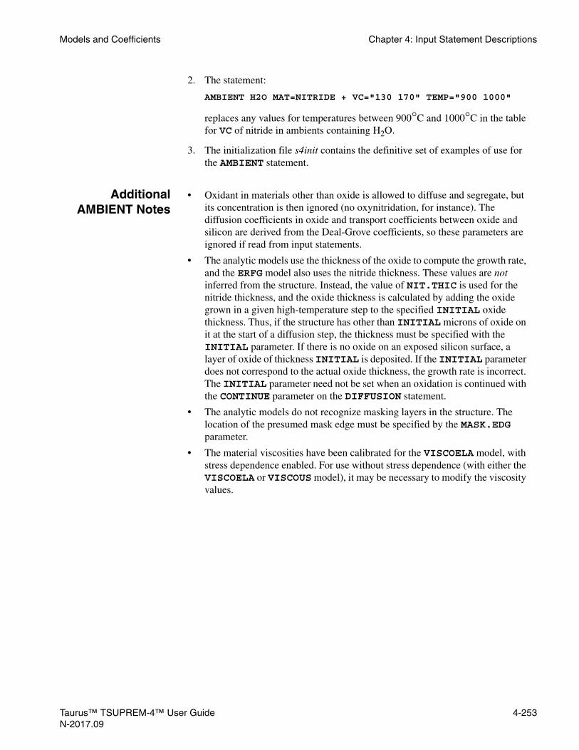
Models and Coefficients Chapter 4: Input Statement Descriptions

2. The statement:

AMBIENT H2O MAT=NITRIDE + VC="130 170" TEMP="900 1000"

replaces any values for temperatures between 900°C and 1000°C in the table for VC of nitride in ambients containing H2O.

3. The initialization file s4init contains the definitive set of examples of use for the AMBIENT statement.

AdditionalAMBIENT Notes

• Oxidant in materials other than oxide is allowed to diffuse and segregate, but its concentration is then ignored (no oxynitridation, for instance). The diffusion coefficients in oxide and transport coefficients between oxide and silicon are derived from the Deal-Grove coefficients, so these parameters are ignored if read from input statements.

• The analytic models use the thickness of the oxide to compute the growth rate, and the ERFG model also uses the nitride thickness. These values are not inferred from the structure. Instead, the value of NIT.THIC is used for the nitride thickness, and the oxide thickness is calculated by adding the oxide grown in a given high-temperature step to the specified INITIAL oxide thickness. Thus, if the structure has other than INITIAL microns of oxide on it at the start of a diffusion step, the thickness must be specified with the INITIAL parameter. If there is no oxide on an exposed silicon surface, a layer of oxide of thickness INITIAL is deposited. If the INITIAL parameter does not correspond to the actual oxide thickness, the growth rate is incorrect. The INITIAL parameter need not be set when an oxidation is continued with the CONTINUE parameter on the DIFFUSION statement.

• The analytic models do not recognize masking layers in the structure. The location of the presumed mask edge must be specified by the MASK.EDG parameter.

• The material viscosities have been calibrated for the VISCOELA model, with stress dependence enabled. For use without stress dependence (with either the VISCOELA or VISCOUS model), it may be necessary to modify the viscosity values.

Taurus™ TSUPREM-4™ User Guide 4-253N-2017.09

Chapter 4: Input Statement Descriptions Models and Coefficients

MOMENT

The MOMENT statement sets distribution moments for use in ion implantation.

MOMENT

[ { MATERIAL=<c> | SILICON | OXIDE | OXYNITRI | NITRIDE | POLYSILI | PHOTORES | ALL.MATE } ]

{ ( [CLEAR] [ { RANGE=<n> SIGMA=<n> [GAMMA=<n>] [KURTOSIS=<n>] [LSIGMA=<n>]

[LSLOPE=<n>] [ { DAMAGE [LAMBDA=<n>] [SCALE=<n>] } ][ { SIMS.FIL=<c>

[ { FIT [TOLERANC=<n>] [MAX.ITER=<n>] [RP.OFFSE=<n>] } ][ { SIMS.NM | SIMS.UM | SIMS.CM } ][SIMS.YCO=<n>] [SIMS.COL=<n>][SIMS.YLO=<n>] [SIMS.YHI=<n>][SIMS.MIN=<n>] [SIMS.MAX=<n>]

}]

[ { D.FRAC=<n> D.RANGE=<n> D.SIGMA=<n> [D.GAMMA=<n>][D.KURTOS=<n>] [D.LSIGMA=<n>] [D.LSLOPE=<n>] } ]

[TILT=<n>] } ] )|( { IMPURITY=<c> | ANTIMONY | ARSENIC | BORON | BF2 | PHOSPHOR }

[GE.EFF][D.SUP.R=<n>] [D.SUP.E=<n>] [RANGE.0=<n>] [RANGE.F=<n>][SIGMA.0=<n>] [SIGMA.F=<n>] [D.RAN.0=<n>] [D.RAN.F=<n>][D.SIG.0=<n>] [D.SIG.F=<n>] [TABLE=<c>] [DAM.TABL=<c>]

)}

Parameter Type Definition

MATERIAL character The name of the material to which the given range statistics apply.Default: none

SILICON logical Specifies that the given range statistics apply to implantation into silicon.Default: true, unless another material is specified

OXIDE logical Specifies that the given range statistics apply to implantation into oxide.Default: false

OXYNITRI logical Specifies that the given range statistics apply to implantation into oxynitride.Default: false

NITRIDE logical Specifies that the given range statistics apply to implantation into nitride.Default: false

POLYSILI logical Specifies that the given range statistics apply to implantation into polysilicon.Default: false

4-254 Taurus™ TSUPREM-4™ User GuideN-2017.09

Models and Coefficients Chapter 4: Input Statement Descriptions

PHOTORES logical Specifies that the given range statistics apply to implantation into photoresist.Default: false

ALL.MATE logical Specifies that the parameter values will be applied to all materials. Applies only to the Taurus Analytic Implant Model.Default: false

CLEAR logical Clears all moments specified on previous MOMENT statements. Default: false

RANGE number The first moment (projected range) of the first Pearson or Gaussian distribution. units: micronsDefault: none

SIGMA number The second moment (standard deviation) of the first Pearson or Gaussian distribution.Units: micronsDefault: none

GAMMA number The third moment ratio (skewness) of the first Pearson distribution.Units: noneDefault: 0.0

KURTOSIS number The fourth moment ratio (kurtosis) of the first Pearson distribution.Units: noneDefault: calculated from the first three moments

LSIGMA number The lateral (perpendicular to the ion beam) standard deviation for the first Pearson or Gaussian distribution.Units: micronsDefault: SIGMA

LSLOPE number The slope of the lateral standard deviation for the first Pearson distribution of the dual-Pearson model.Units: micronsDefault: 0.0

DAMAGE logical Specifies that the remaining parameters on the MOMENT statement are used for damage calculation. In particular, RANGE and SIGMA specify Hobler’s a2 and a3 parameters. LSIGMA and LSLOPE specify the lateral spread and depth dependence of the lateral spread for the damage model. Default: false

LAMBDA number The slope of the exponential part of the damage profile (Hobler’s a1 parameter). Units: microns-1

Default: value taken from implant damage moments file or built-in model.

SCALE number The damage scaling factor (Hobler’s nv[] parameter; related to the number of Frenkel pairs created for each implanted dopant ion). Units: noneDefault: value taken from implant damage moments file or built-in model.

Parameter Type Definition

Taurus™ TSUPREM-4™ User Guide 4-255N-2017.09

Chapter 4: Input Statement Descriptions Models and Coefficients

SIMS.FIL character The file name of the SIMS data to be loaded to generate the as-implant profiles for the IMPLANT statements with MOMENT. Applies only to the Taurus Analytic Implant Model.Default: none

FIT logical Specifies to extract the dual Pearson moments from the SIMS.FIL data, and to use the extracted moments to generate the as-implant profiles for the IMPLANT statements with MOMENT.Default: false

TOLERANC number Error tolerance for convergence to extract the dual Pearson moments from the SIMS.FIL data. Only applicable when FIT is turned on.Units: %Default: 0.1

MAX.ITER number Maximum number for iteration to extract the dual Pearson implant moments from the SIMS.FIL data. Only applicable when FIT is turned on.Units: noneDefault: 500

RP.OFFSE number The offset value for the projected ranges of the first and second Pearson moments. The extracted projected ranges are shifted by RP.OFFSE. Only applicable when FIT is turned on.Units: micronsDefault: 0.0

SIMS.NM logical Specifies that the unit of the depth data in the SIMS.FIL file is nanometers.Default: false

SIMS.UM logical Specifies that the unit of the depth data in the SIMS.FIL file is microns.Default: true

SIMS.CM logical Specifies that the unit of the depth data in the SIMS.FIL file is centimeters.Default: false

SIMS.YCO number The column number of the depth data in the SIMS.FIL file.Units: noneDefault: 1

SIMS.COL number The column number of the concentration data in the SIMS.FIL file.Units: noneDefault: 2

SIMS.YLO number The lowest value of the depth data to be loaded from the SIMS.FIL file. The SIMS data in the range within (SIMS.YLO, SIMS.MIN) and (SIMS.YHI, SIMS.MAX) are selected for generating as-implanted profiles. The nearest depth to SIMS.YLO location is mapped to the top surface of the MATERIAL region.Units: nanometers for SIMS.NM, or microns for SIMS.UM, or centimeters for SIMS.CMDefault: the first value of the depth data in SIMS.FILSynonym: SIMS.YOF

Parameter Type Definition

4-256 Taurus™ TSUPREM-4™ User GuideN-2017.09

Models and Coefficients Chapter 4: Input Statement Descriptions

SIMS.YHI number The highest value of the depth data to be loaded from the SIMS.FIL file. The SIMS data in the range within (SIMS.YLO, SIMS.MIN) and (SIMS.YHI, SIMS.MAX) are to be imported.Units: nanometers for SIMS.NM, or microns for SIMS.UM, or centimeters for SIMS.CMDefault: 1x1010

SIMS.MIN number The minimum value of the concentration data to be loaded from the SIMS.FIL file. The SIMS data in the range within (SIMS.YLO, SIMS.MIN) and (SIMS.YHI, SIMS.MAX) are loaded to extract the moments.Units: cm-3

Default: 1x1014

SIMS.MAX number The maximum value of the concentration data to be loaded from the SIMS.FIL file. The SIMS data in the range within (SIMS.YLO, SIMS.MIN) and (SIMS.YHI, SIMS.MAX) are loaded to extract the moments.Units: cm-3

Default: 1x1030

D.FRAC number The fraction of the implant dose that uses the first Pearson distribution of the dual-Pearson model.units: micronsDefault: none

D.RANGE number The first moment (projected range) of the second Pearson distribution of the dual-Pearson model.units: micronsDefault: none

D.SIGMA number The second moment (standard deviation) of the second Pearson distribution of the dual-Pearson model.Units: micronsDefault: none

D.GAMMA number The third moment ratio (skewness) of the second Pearson distribution of the dual-Pearson model.Units: noneDefault: 0.0

D.KURTOS number The fourth moment ratio (kurtosis) of the second Pearson distribution of the dual-Pearson model.Units: noneDefault: calculated from the first three moments

D.LSIGMA number The lateral (perpendicular to the ion beam) standard deviation for the second Pearson distribution of the dual-Pearson model.Units: micronsDefault: D.SIGMA

Parameter Type Definition

Taurus™ TSUPREM-4™ User Guide 4-257N-2017.09

Chapter 4: Input Statement Descriptions Models and Coefficients

D.LSLOPE number The slope of the lateral standard deviation for the second Pearson distribution of the dual-Pearson model.Units: micronsDefault: 0.0

TILT number The angle between the direction of the ion beam and direction along which the specified moments are measured.Units: degreesDefault: 0.0

IMPURITY character The name of the impurity for which the Taurus Analytic Implant Model parameter values are set. Applies only to the Taurus Analytic Implant Model.Default: noneSynonym: IMP

ANTIMONY logical Specifies that the Taurus Analytic Implant Model parameter values are set for antimony. Applies only to the Taurus Analytic Implant Model.Default: false Synonym: SB

ARSENIC logical Specifies that the Taurus Analytic Implant Model parameter values are set for arsenic. Applies only to the Taurus Analytic Implant Model.Default: false Synonym: AS

BORON logical Specifies that the Taurus Analytic Implant Model parameter values are set for boron. Applies only to the Taurus Analytic Implant Model. Default: false Synonym: B

BF2 logical Specifies that the Taurus Analytic Implant Model parameter values are set for boron in the form of BF2. Applies only to the Taurus Analytic Implant Model.Default: false

PHOSPHOR logical Specifies that the Taurus Analytic Implant Model parameter values are set for phosphorus. Applies only to the Taurus Analytic Implant Model. Default: false Synonym: P

GE.EFF logical Specifies that the Taurus Analytic Implant Model parameter values, D.SUP.R, D.SUP.E, RANGE.0, RANGE.F, SIGMA.0, SIGMA.F, D.RAN.0, D.RAN.F, D.SIG.0 and D.SIG.F are set for Ge-Dependent Reshaping Model. Applies only to the Taurus Analytic Implant Model.Default: false

D.SUP.R number Sets the value of the MINRATIO parameter in the Effective Channeling Suppression Model for the specified material and impurity. Applies only to the Taurus Analytic Implant Model. Units: noneDefault: the current value for the specified impurities and materials

Parameter Type Definition

4-258 Taurus™ TSUPREM-4™ User GuideN-2017.09

Models and Coefficients Chapter 4: Input Statement Descriptions

D.SUP.E number Sets the value of the EXPONENT parameter in the Effective Channeling Suppression Model for the specified material and impurity. Applies only to the Taurus Analytic Implant Model.Units: noneDefault: the current value for the specified impurities and materials

RANGE.0 number Sets the prefactor value for the range shift of the 1st Pearson profile in Ge-Dependent Reshaping Model for the specified material and impurity. Applies only to the Taurus Analytic Implant Model.Units: micronsDefault: the current value for the specified impurities and materials

RANGE.F number Sets the value of the RANGEFACTOR parameter in the Profile Reshaping Model or Ge-Dependent Reshaping Model for the specified material and impurity. Applies only to the Taurus Analytic Implant Model.Units: noneDefault: the current value for the specified impurities and materials

SIGMA.0 number Sets the prefactor value for the standard deviation change of the 1st Pearson profile in Ge-Dependent Reshaping Model for the specified material and impurity. Applies only to the Taurus Analytic Implant Model.Units: micronsDefault: the current value for the specified impurities and materials

SIGMA.F number Sets the value of the SIGMAFACTOR parameter in the Profile Reshaping Model or Ge-Dependent Reshaping Model for the specified material and impurity. Applies only to the Taurus Analytic Implant Model.Units: noneDefault: the current value for the specified impurities and materials

D.RAN.0 number Sets the prefactor value for the range shift of the 2nd Pearson profile in Ge-Dependent Reshaping Model for the specified material and impurity. Applies only to the Taurus Analytic Implant Model.Units: micronsDefault: the current value for the specified impurities and materials

D.RAN.F number Sets the value of the CHANNELINGRANGEFACTOR parameter in the Profile Reshaping Model or Ge-Dependent Reshaping Model for the specified material and impurity. Applies only to the Taurus Analytic Implant Model.Units: noneDefault: the current value for the specified impurities and materials

D.SIG.0 number Sets the prefactor value for the standard deviation change of the 2nd Pearson profile in Ge-Dependent Reshaping Model for the specified material and impurity. Applies only to the Taurus Analytic Implant Model.Units: micronsDefault: the current value for the specified impurities and materials

Parameter Type Definition

Taurus™ TSUPREM-4™ User Guide 4-259N-2017.09

Chapter 4: Input Statement Descriptions Models and Coefficients

Description The MOMENT statement specifies moments to be used by the ion implantation model. The values specified by MOMENT statements are used instead of values in the implant data file s4imp0 on IMPLANT statements that specify the MOMENTS parameter.

One full set of moments for the Gaussian, single Pearson, or dual Pearson implant model can be specified for each material. A MOMENT statement for a particular material replaces any previously specified moments for that material. The CLEAR parameter clears any user specified moment data for all materials.

When the MOMENTS parameter is specified on an IMPLANT statement, values specified on MOMENT statements are used for materials for which MOMENT statements were given. Moments for other materials are obtained from the moments data file, as usual.

Optional andRequired Model

Parameters

The models or the MOMENT parameter have mandatory and optional parameters. They are listed below.

• For the Gaussian implant model, RANGE and SIGMA must be specified, and LSIGMA is optional.

• For the (single) Pearson model, RANGE, and SIGMA must be specified, and GAMMA, LSIGMA, and KURTOSIS are optional.

• For the dual Pearson model, the D.FRAC, D.RANGE, and D.SIGMA parameters must be specified in addition to the parameters of the single Pearson model; D.GAMMA, D.LSIGMA, and D.KURTOS are optional.

• The TILT parameter is optional.

D.SIG.F number Sets the value of the CHANNELINGSIGMAFACTOR parameter in the Profile Reshaping Model or Ge-Dependent Reshaping Model for the specified material and impurity. Applies only to the Taurus Analytic Implant Model.Units: noneDefault: the current value for the specified impurities and materials

TABLE character Sets the default value of the file name suffix for the implant tables which contain the desired implant data in the format of ION_IN_MATERIAL_SUFFIX. This parameter changes the default suffix for all materials. Use the DATA.SUF parameter of the IMPLANT command to change the suffix for a single process step. Applies only to the Taurus Analytic Implant Model.Default: STANDARD

DAM.TABL character Sets the default value of the file name suffix for the implant tables which contain the desired implant damage data in the format of ION_DAMAGE_IN_MATERIAL_SUFFIX. This parameter changes the default suffix for all materials. Use the DAM.SUF parameter of the IMPLANT command to change the suffix for a single process step. Applies only to the Taurus Analytic Implant Model.Default: STANDARD

Parameter Type Definition

4-260 Taurus™ TSUPREM-4™ User GuideN-2017.09

Models and Coefficients Chapter 4: Input Statement Descriptions

Using theMOMENT

Statement

The MOMENT statement makes it easy to experiment with different implant distribution parameters or to specify alternate parameters for critical implant steps. However, if a particular set of moments is needed frequently, it is easier to create an alternate moment data file.

When the MOMENTS parameter is specified on an IMPLANT statement, moments from preceding MOMENT statements are used without regard to the implant energy or species being implanted. It is your responsibility to ensure that the moments are appropriate for the implant being simulated.

The TILT parameter specifies the angle between the direction of the ion beam during implant and the direction along which the specified moments were (or would be) measured. In a typical experiment, ions are implanted into a tilted wafer and the resulting dopant distribution is measured perpendicular to the surface. If the moments of the measured distribution are specified on the MOMENT statement, then the tilt of the wafer during the implant should be specified by the TILT parameter.

Modifiable HoblerDamage Moments

You now can specify the parameters of the implant damage model on the MOMENT statement or in a table contained in a file. The implant damage model has been extended to allow the lateral spread of the damage profile to be different from the vertical spread and to vary (linearly) with depth. Parameters for the implant damage model come from one of the following sources:

• The MOMENT DAMAGE statement can be used to specify the RANGE, SIGMA, LAMBDA, LSIGMA, LSLOPE, and SCALE parameters used by the damage implant model. LAMBDA specifies the location and slope of the exponential tail of the damage profile, and SCALE specifies the magnitude of the profile. The remaining parameters have the same meaning as the for the Gaussian model for implanted doping profiles. Parameters specified with MOMENT DAMAGE are used on subsequent IMPLANT statements that specify the MOMENTS parameter. Parameters not specified on a MOMENT DAMAGE statement are obtained from one of the following sources. A MOMENT CLEAR statement or a MOMENT DAMAGE statement with no model parameters cancels the effects of any preceding MOMENT DAMAGE statement.

• If DAM.TABL is specified on the IMPLANT statement or on an IMPURITY statement for the implanted dopant, damage parameters are taken from the specified table in an implant damage moments file. The file must be specified on the DAM.FILE parameter on the IMPLANT statement, by the S4IDAM environment variable; otherwise the file named “s4idam” in the current working directory is used. The format of the implant damage moments file is described below. A DAM.TABL specified on an IMPLANT statement takes precedence over DAM.TABL specified on an IMPURITY statement.

Damage parameters not specified on a DAMAGE MOMENT statement or in a damage moments file are calculated from the built-in model of Hobler, as in previous releases of TSUPREM-4. LSIGMA is assumed to be the same as SIGMA and LSLOPE is zero. The Hobler’s model ignores the exponential tail of the damage profile at low energies for light ions. This is only done if LAMBDA is obtained from the built-in model; if you specify LAMBDA in a MOMENT DAMAGE

Taurus™ TSUPREM-4™ User Guide 4-261N-2017.09

Chapter 4: Input Statement Descriptions Models and Coefficients

statement or in an implant damage moments file, the specified value is used to compute the exponential tail regardless of the implant energy or ion type.

Using SIMS Data For Taurus Analytic Implant Model, the vertical as-implanted profile can be generated not only by the built-in dual Pearson model, but also by directly importing the measured SIMS data. The file including the SIMS data is specified by the SIMS.FIL parameter. The data format in the SIMS.FIL data must be columnwise and listed in ascending order of the depth. For the lateral profile, if the SIMS.FIL is specified with the parameters for the lateral moments, the parameters are used to generate the lateral profile. Otherwise, the lateral moments are taken from the built-in moment tables for the given implant condition. The following example shows how to directly import the SIMS data for vertical profile when you have the file, boron_1E14_30kev.dat for the boron SIMS data,

MOMENT SILICON SIMS.FIL=boron_1E14_30kev.datIMPLANT BORON DOSE=1E14 ENERGY=30 NAME=taurus MOMENT

Since SIMS data necessarily shows the noisy profile for the comparatively low concentration data in the tail region, you may want to discard such noisy data below certain depth. For example, if you want to exclude the data below 0.3 um. The depth unit of the SIMS data is assumed to be microns by default.

MOMENT SILICON SIMS.FIL=boron_1E14_30kev.dat +SIMS.YHI=0.3

When the depth unit in the SIMS data is nanometers:

MOMENT SILICON SIMS.FIL=boron_1E14_30kev.dat +SIMS.YHI=300 SIMS.NM

When the measured data near surface indicates the oxide layer on the top of silicon substrate so that you want to exclude the data, SIMS.YLO can be defined to the interface location, for example, 20 angstroms, between oxide and silicon.

MOMENT SILICON SIMS.FIL=boron_1E14_30kev.dat +SIMS.YHI=0.3 SIMS.YLO=0.002

Note:The SIMS data at SIMS.YLO is imported to the surface location of the specified material in the simulation structure.

Direct import of SIMS data has an advantage of using the real measured data for implantation simulations, thereby improving the simulation accuracy. Although it does not require any moment to generate an implant profile, the projected range is necessary for the RP.EFF model to determine the effective thickness of the multiple layers on the top of the region into which the SIMS data is imported. The projected range can be given by the RANGE parameter. Otherwise, TSUPREM-4 calculates the projected range from the SIMS data.

$ CASE1MOMENT SI RANGE=0.06 SIMS.FIL=boron.datINITDEPOSIT OXIDE THICKNES=0.01 IMPLANT BORON DOSE=1E14 ENERGY=30 NAME=taurus MOMENT

4-262 Taurus™ TSUPREM-4™ User GuideN-2017.09

Models and Coefficients Chapter 4: Input Statement Descriptions

According to the RP.EFF model, the following example shows the same shape of the boron profiles in silicon as the above case:

$ CASE2MOMENT SI RANGE=0.06*0.5 SIMS.FIL=boron.datINITDEPOSIT OXIDE THICKNES=0.01*2 IMPLANT BORON DOSE=1E14 ENERGY=30 NAME=taurus MOMENT

There are some models such as PAI which are tightly coupled with the profile model, so it is not possible to apply such models when the as-implant profile is generated by the direct use of SIMS data. Turning on the FIT parameter specifies to internally extract the dual Pearson parameters from a given SIMS data, and to use the dual Pearson model instead of the measured data itself. For example:

MOMENT SI SIMS.FIL=boron.dat SIMS.YHI=0.3 FIT

The above command prints out the optimization procedure to extract the dual Pearson parameters and the extracted moments, for example:

1 rms error = 5.52005 2 rms error = 4.34979 3 rms error = 1.25713 4 rms error = 0.923481 5 rms error = 0.595509 6 rms error = 0.351398 7 rms error = 0.186888 8 rms error = 0.183109 9 rms error = 0.18286 10 rms error = 0.181501 11 rms error = 0.18122 12 rms error = 0.181193 13 rms error = 0.181188

material Rp sigma gamma beta fraction Si 0.07054 0.03928 0.3521 2.24 0.1997 (dual) 0.04787 0.05081 -0.4416 3.443 0.8003

Thus, the following two examples generate the identical boron profiles:

$ Case1INITMOMENT SI SIMS.FIL=boron.dat SIMS.YHI=0.3 FITIMPLANT BORON DOSE=1E14 ENERGY=10 NAME=taurus MOMENT

$ Case2INITMOMENT SI RANGE=0.07054 SIGMA=0.03928 GAMMA=0.3521 +

KURTOSIS=2.24 D.RANGE=0.04787 D.SIGMA=0.05081 +D.GAMMA=-0.4416 D.KURTOS=3.443 D.FRAC=0.1997

IMPLANT BORON DOSE=1E14 ENERGY=10 NAME=taurus MOMENT

Taurus™ TSUPREM-4™ User Guide 4-263N-2017.09

Chapter 4: Input Statement Descriptions Models and Coefficients

Examples 1. In the following series of statements:

MOMENT SILICON RANGE=0.195 SIGMA=0.072 GAMMA=-0.65 +KURTOSIS=22.1

IMPLANT BORON DOSE=1e15 ENERGY=70 MOMENTS

The implantation of boron into silicon uses the (single) Pearson distribution specified on the MOMENT statement. In materials other than silicon, distribution parameters from the implant data file are used.

2. In the statement:

IMPLANT ARSENIC DOSE=2e15 ENERGY=40

parameters for the arsenic distribution come from the implant data file. Parameters specified on MOMENT statements are not used because MOMENTS is not specified on the IMPLANT statement.

Additional Notes The implanted dose in the silicon is reduced by the dose that is stopped in screening layers or backscattered from the surface, and thus depends weakly on the implant moments in the screening layer. Because the calculated damage is proportional to the dose in the silicon, the amount of damage is also weakly dependent on the moments in the screening layer.

4-264 Taurus™ TSUPREM-4™ User GuideN-2017.09

Models and Coefficients Chapter 4: Input Statement Descriptions

MATERIAL

The MATERIAL statement sets the physical properties of materials.

MATERIAL { ( MATERIAL=<c> [NEW])| SILICON | OXIDE | OXYNITRI | NITRIDE | POLYSILI | PHOTORES | ALUMINUM | AMBIENT } [TIF.NAME=<c>] [MD.INDEX=<n>] [IMPL.TAB=<c>] [DY.DEFAU=<n>] [E.FIELD] [ION.PAIR] [IP.OMEGA=<n>]

[NI.0=<n>] [NI.E=<n>] [NI.F=<n>] [EG.ADD=<c> [MODEL=<c>]] [EPSILON=<n>] [DENSITY=<n>] [AT.RADIU=<n>][VISC.0=<n>] [VISC.E=<n>] [VISC.X=<n>] [VC=<c>] [TEMPERAT=<c>]

[YOUNG.M=<n>] [POISS.R=<n>] [LCTE=<c>][INTRIN.S=<n>] [SURF.TEN=<n>] [STRENGTH=<n>][C11.0=<n>] [C12.0=<n>] [C44.0=<n>][C11.1=<n>] [C12.1=<n>] [C44.1=<n>] [ANISOEL]

[ { (SEMICOND [AFFINITY=<n>] [BANDGAP=<n>] [EGALPH=<n>] [EGBETA=<n>] [N.CONDUC=<n>] [N.VALENC=<n>] [NC.F=<n>] [NV.F=<n>] [G.DONOR=<n>] [E.DONOR=<n>] [G.ACCEP=<n>] [E.ACCEP=<n>] [BOLTZMAN] [IONIZATI] [QM.BETA=<n>] [QM.YCRIT=<n>]) | ( CONDUCTO [WORKFUNC=<n>] ) } ]

[MAX.DAMA=<n>] [DAM.GRAD=<n>] [D.PCONST=<n>] [D.PME=<n>] [D.PDLF=<n>][D.PDLME=<n>] [D.PDRE=<n>] [D.PNORM=<n>] [D.PDE=<n>] [D.PHDF=<n>][D.PME=<n>] [D.PLF=<n>] [D.PLME=<n>]

[POLYCRYS] [GRASZ.0=<n>] [GRASZ.E=<n>] [TEMP.BRE=<n>] [MIN.GRAI=<n>] [FRAC.TA=<n>] [G.DENS=<n>] [F11=<n>] [F22=<n>] [ALPHA=<n>] [GEOM=<n>] [GAMMA.0=<n>] [GAMMA.E=<n>] [DSIX.0=<n>] [DSIX.E=<n>] [DSIM.0=<n>] [DSIM.E=<n>] [DSIMM.0=<n>] [DSIMM.E=<n>] [DSIP.0=<n>] [DSIP.E=<n>] [GBE.0=<n>] [GBE.H=<n>] [GBE.E=<n>] [NSEG=<n>] [TBU.0=<n>] [TBU.E=<n>] [TOXIDE=<n>] [EAVEL.0=<n>] [EAVEL.E=<n>] [DLGX.0=<n>] [DLGX.E=<n>] [GB.THICK=<n>]

[N.SPECIE=<n>] [AT.NUM=<n>] [AT.WT=<n>] [MOL.WT=<n>][AT.WT.1=<n>] [AT.WT.2=<n>] [AT.WT.3=<n>] [AT.NUM.1=<n>] [AT.NUM.2=<n>] [AT.NUM.3=<c>][AT.NAM.1=<c>] [AT.NAM.2=<c>] [AT.NAM.3=<c>] [STOICH.1=<n>][STOICH.2=<n>][STOICH.3=<n>][ABUND.1=<n>] [ABUND.2=<n>] [ABUND.3=<n>] [DEBYE.T=<n>] [AMOR.THR=<n>][MC.GE.MI=<n>] [SURF.DIS=<n>] [D.SIM=<n>] [V.RAN.D=<n>][AMORPH | POLY.MC | (CRYSTAL [LATT.A=<n>][SC | BCC | FCC | DIAMOND | HEXAGON])] [POLY.ORI=<n>] [POLY.GSZ=<n>] [POLY.FAC=<n>][SIC.2H | SIC.3C | SIC.4H | SIC.6H][EPI.ANGL=<c>] [EPI.RATE=<c>]

[EQACT.IN]

Taurus™ TSUPREM-4™ User Guide 4-265N-2017.09

Chapter 4: Input Statement Descriptions Models and Coefficients

Parameter Type Definition

MATERIAL character The following parameters apply to the named material. Default: none Synonym: NAME

NEW logical Used to define a new material. The name specified by the MATERIAL parameter must not have been previously used as a material name.Default: false

SILICON logical The following parameters apply to silicon. Default: false

OXIDE logical The following parameters apply to oxide. Default: false

OXYNITRI logical The following parameters apply to oxynitride. Default: false

NITRIDE logical The following parameters apply to nitride. Default: false

POLYSILI logical The following parameters apply to polysilicon. Default: false Synonym: POLY

PHOTORES logical The following parameters apply to photoresist. Default: false

ALUMINUM logical The following parameters apply to aluminum. Default: false

AMBIENT logical The following parameters apply to ambient.Default: false Synonym: GAS

TIF.NAME character The name by which this material is known in the TIF materials database.Note: This value of this parameter is case-sensitive.Default: the name of the material

MD.INDEX number The index to be used for this material when saving the structure in Medici file format. These correspond to the <matx> indices listed in Appendix D. Units: noneDefault: 0 (material ignored by Medici)

IMPL.TAB character The name of the material in the implant moment file to be associated with this material.Default: the current value for this material; initially the name of the material

DY.DEFAU number The grid spacing to be used in growing layers of the material. This value is scaled by the value of the GRID.FAC parameter on the METHOD statement. A value of zero specifies that no grid is to be added in growing layers.Units: micronsDefault: the current value; initially 0.0Synonym: DX.DEFAU

4-266 Taurus™ TSUPREM-4™ User GuideN-2017.09

Models and Coefficients Chapter 4: Input Statement Descriptions

E.FIELD logical Specifies that the electric field terms are to be included in the impurity diffusion equations for this material. (Meaningful only for silicon and polysilicon.)Default: the current value for this material; initially true

ION.PAIR logical Enables the model for pairing between donor and acceptor ions in this material.Default: the current value for this material; initially true for silicon and polysilicon

IP.OMEGA number The multiple of the intrinsic carrier concentration at which ion pairing becomes significant in this material.Units: noneDefault: the current value for this material; initially 6.0 for silicon and polysilicon

NI.0 number The prefactor in the expression for the intrinsic carrier concentration. Units: carriers/cm3*(degrees Kelvin)NI.F Default: the current value for this material; initially 3.87e16

NI.E number The activation energy in the expression for the intrinsic carrier concentration. Units: electron volts Default: the current value for this material; initially 0.605

NI.F number The temperature exponent in the expression for the intrinsic carrier concentration. Units: none Default: the current value for this material; initially 1.5Synonym: NI.POW

EG.ADD character The expression of the energy bandgap changeUnits: electron volts Default: 0.0

MODEL character The model name for the expression EG.ADD of the energy bandgap changeDefault: None

EPSILON number The relative permittivity of the material. Units: none Default: the current value for this material; see Appendix A for initial values

DENSITY number The density of the material. Units: gm/cm3 Default: the current value; see Appendix A for initial values.

AT.RADIU number Atom covalent radius. Used for calculating the misfit strain when one of the DEPO.MIS or DIFF.MIS or STN.MIS parameters is turned on.Units: angstromsDefault: the current value; see Appendix A for initial values.

VISC.0 number The exponential prefactor for the viscosity. Units: gm/(cm*s) Default: the current value for this material

Parameter Type Definition

Taurus™ TSUPREM-4™ User Guide 4-267N-2017.09

Chapter 4: Input Statement Descriptions Models and Coefficients

VISC.E number The activation energy for the viscosity. Units: electron volts Default: the current value for this material

VISC.X number The incompressibility factor. A value of 0.5 corresponds to an infinitely incompressible material. The value must be strictly less than 0.5.Units: none Default: the current value for this material

VC character A table of activation volumes as a function of temperature for the dependence of material viscosity on shear stress for the specified material in inert-ambient diffusions. Entries in the table correspond to temperatures given by the TEMPERAT parameter (see text).Units: Å3 Default: the current value for this material

TEMPERAT character A list of temperatures corresponding to the values of the VC parameter.Units: degrees CelsiusDefault: none

YOUNG.M number Young’s modulus for the material. Units: dynes/cm2 Default: the current value for this material

POISS.R number Poisson ratio for the material. Units: none Default: the current value for this material

LCTE character An expression giving the linear coefficient of thermal expansion as a function of absolute temperature, called T in the expression. It is given as a fraction, not as a percentage. Units: none Default: the current value for this material

INTRIN.S number The initial uniform stress state of a material, such as a thin film of nitride deposited on the substrate. Units: dynes/cm2 Default: the current value for this material

SURF.TEN number The surface tension for this material. Affects reflow during oxidation with the VISCOUS model. Units: dynes/cm Default: the current value for this material

STRENGTH number The maximum absolute stress value for this material.Units: dynes/cm2 Default: the current value for this material; initially YOUNG.M/20.0

ANISOEL logical Specifies that the material is anisotropically elastic.Default: false

Parameter Type Definition

4-268 Taurus™ TSUPREM-4™ User GuideN-2017.09

Models and Coefficients Chapter 4: Input Statement Descriptions

C11.0 number The elastic constant Sxx/Exx in crystallographic axes.Units: dynes/cm2 Default: the current value for this material

C11.1 number The first-order temperature dependence of the elastic constant Sxx/Exx in crystallographic axes.Units: dynes/cm2/oKDefault: the current value for this material

C12.0 number The elastic constant Sxx/Eyy in crystallographic axes.Units: dynes/cm2 Default: the current value for this material

C12.1 number The first-order temperature dependence of the elastic constant Sxx/Eyy in crystallographic axes.Units: dynes/cm2/oKDefault: the current value for this material

C44.0 number The elastic constant Sxy/Exy in crystallographic axes.Units: dynes/cm2 Default: the current value for this material

C44.1 number The first-order temperature dependence of the elastic constant Sxy/Exy in crystallographic axes.Units: dynes/cm2/oKDefault: the current value for this material

SEMICOND logical Specifies that the material is a semiconductor.Default: false

AFFINITY number The electron affinity of the material.Units: electron voltsDefault: the current value for this material

BANDGAP number The energy band gap of the material.Units: electron voltsDefault: the current value for this material

EGALPH number The value of alpha used in calculating the energy bandgap as a function of temperature.Units: eV/KelvinDefault: the current value for this material

EGBETA number The value of beta used in calculating the energy bandgap as a function of temperature.Units: KelvinsDefault: the current value for this material

N.CONDUC number The effective density of electron states in the conduction band of the material at 300°K.Units: #/cm3

Default: the current value for this material

Parameter Type Definition

Taurus™ TSUPREM-4™ User Guide 4-269N-2017.09

Chapter 4: Input Statement Descriptions Models and Coefficients

N.VALENC number The effective density of hole states in the valence band of the material at 300°K.Units: #/cm3

Default: none

NC.F number The exponent of the temperature dependence for the effective density of electron states in the conduction band of the material.Units: noneDefault: the current value for this material

NV.F number The exponent of the temperature dependence for the effective density of hole states in the valence band of the material.Units: noneDefault: the current value for this material

G.DONOR number The donor impurity degeneracy factor of the material.Units: noneDefault: the current value for this material

E.DONOR number The donor impurity ionization energy of the material.Units: electron voltsDefault: the current value for this material

G.ACCEP number The acceptor impurity degeneracy factor of the material.Units: noneDefault: the current value for this material

E.ACCEP number The acceptor impurity ionization energy of the material.Units: electron voltsDefault: the current value for this material

BOLTZMAN logical Specifies that Boltzmann carrier statistics are used for this material during electrical calculations. If this parameter is false, Fermi-Dirac statistics are used.Default: the current value for this material

IONIZATI logical Specifies that complete impurity ionization is used for this material during electrical calculations. If this parameter is false, the impurities are considered to be incompletely ionized.Default: the current value for this material

QM.BETA number The proportional factor for van Dort’s QM modeling.Units: eVcmDefault: the current value for this material

QM.YCRIT number The critical depth of quantization for van Dort’s QM modeling.Default: the current value for this material

CONDUCTO logical Specifies that the material is a conductor.Default: false

WORKFUNC number The work function of the material.Units: electron voltsDefault: the current value for this material

Parameter Type Definition

4-270 Taurus™ TSUPREM-4™ User GuideN-2017.09

Models and Coefficients Chapter 4: Input Statement Descriptions

MAX.DAMA number The damage threshold for amorphization of this material.Synonym: AMOR.THRUnits: #/cm3 Default: the current value for this material; initially 1.15×1022 for silicon

DAM.GRAD number The sharpness of the amorphous/single-crystal interface in this material following solid-phase epitaxial regrowthUnits: noneDefault: the current value for this material; initially 10 for silicon

D.PCONST number An empirical constant for the effective +n implant damage model.Units: noneDefault: the current value for this material; initially 3.25 for silicon

D.PDME number The mass exponent in the low dose factor for the effective +n implant damage model.Units: noneDefault: the current value for this material; initially –0.5 for silicon

D.PDLF number The prefactor for lambda in the low dose factor for the effective +n implant damage model.Units: noneDefault: the current value for this material; initially –2 for silicon

D.PDLME number The mass exponent in lambda in the low dose factor for the effective +n implant damage model.Units: noneDefault: the current value for this material; initially –0.5 for silicon

D.PDRE number The projected range exponent in the low dose factor for the effective +n implant damage model.Units: noneDefault: the current value for this material; initially 0 for silicon

D.PNORM number The normalization for dose for the effective +n implant damage model.Units: #/cm3

Default: the current value for this material; initially 3e12 for silicon

D.PDE number The dose exponent for the effective +n implant damage model.Units: noneDefault: the current value for this material; initially 1.0 for silicon

D.PHDF number The constant in the high dose factor for the effective +n implant damage model.Units: noneDefault: the current value for this material; initially 0.0905 for silicon

D.PME number The mass exponent in the high dose factor for the effective +n implant damage model.Units: noneDefault: the current value for this material; initially 0.85 for silicon

Parameter Type Definition

Taurus™ TSUPREM-4™ User Guide 4-271N-2017.09

Chapter 4: Input Statement Descriptions Models and Coefficients

D.PLF number The prefactor for lambda in the high dose factor for the effective +n implant damage model.Units: noneDefault: the current value for this material; initially –2 for silicon

D.PLME number The mass exponent in lambda in the high dose factor for the effective +n implant damage model.Units: noneDefault: the current value for this material; initially –0.5 for silicon

POLYCRYS logical Specifies that the polycrystalline diffusion and grain-growth models are to be used for this material.Default: the current value for this material; initially true for polysilicon

GRASZ.0 number The pre-exponential factor for the as-deposited grain size during polycrystalline (high-temperature) deposition.Units: noneDefault: the current value for this material

GRASZ.E number The activation energy for the as-deposited grain size during polycrystalline (high-temperature) deposition.Units: electron voltsDefault: the current value for this material

TEMP.BRE number The threshold temperature for amorphous deposition; deposition is amorphous at lower temperatures and polycrystalline at higher temperatures.Units: °CelsiusDefault: the current value for this material

MIN.GRAI number The minimum as-deposited grain size.Units: micronsDefault: the current value for this material

FRAC.TA number The geometrical factor for recrystallized grain size in amorphous regions.Units: noneDefault: the current value for this material

G.DENS number The geometrical factor for the density of grain boundaries.Units: noneDefault: the current value for this material; initially 2.0 for polysilicon

F11 number The geometrical factor for grain-boundary diffusion perpendicular to the columnar direction.Units: noneDefault: the current value for this material; initially 1.0 for polysilicon

F22 number The geometrical factor for grain-boundary diffusion parallel to the columnar direction.Units: noneDefault: the current value for this material; initially 2.0 for polysilicon

Parameter Type Definition

4-272 Taurus™ TSUPREM-4™ User GuideN-2017.09

Models and Coefficients Chapter 4: Input Statement Descriptions

ALPHA number The geometrical factor relating the average grain boundary velocity to the grain growth rate.Units: noneDefault: the current value for this material; initially 1.33 for polysilicon

GEOM number The geometrical factor for the grain growth rate.Units: noneDefault: the current value for this material; initially 6.0 for polysilicon

GAMMA.0 number Pre-exponential factor for the enhancement of silicon self-diffusivity at grain boundaries.Units: noneDefault: the current value for this material

GAMMA.E number Activation energy for the enhancement of silicon self-diffusivity at grain boundaries.Units: electron voltsDefault: the current value for this material

DSIX.0 number Pre-exponential factor for the neutral component of silicon self diffusivity.Units: cm2/sDefault: the current value for this material

DSIX.E number Activation energy for the neutral component of silicon self diffusivity.Units: electron voltsDefault: the current value for this material

DSIM.0 number Pre-exponential factor for the singly negative component of silicon self-diffusivity.Units: cm2/sDefault: the current value for this material

DSIM.E number Activation energy for the singly negative component of silicon self-diffusivity.Units: electron voltsDefault: the current value for this material

DSIMM.0 number Pre-exponential factor for the doubly-negative component of silicon self-diffusivity.Units: cm2/sDefault: the current value for this material

DSIMM.E number Activation energy for the doubly-negative component of silicon self-diffusivity.Units: electron voltsDefault: the current value for this material

DSIP.0 number Pre-exponential factor for the singly-positive component of silicon self-diffusivity.Units: cm2/sDefault: the current value for this material

DSIP.E number Activation energy for the singly-positive component of silicon self-diffusivity.Units: electron voltsDefault: the current value for this material

Parameter Type Definition

Taurus™ TSUPREM-4™ User Guide 4-273N-2017.09

Chapter 4: Input Statement Descriptions Models and Coefficients

GBE.0 number The grain boundary energy for normal grain growth.Units: electron voltsDefault: the current value for this material

GBE.H number The geometrical factor for the reduction of grain growth rate at large grain sizes.Units: noneDefault: the current value for this material

GBE.1 number The grain boundary energy for secondary grain growth.Units: electron voltsDefault: the current value for this material

NSEG number The exponent for solute drag on grain growth.Units: noneDefault: the current value for this material

TBU.0 number The prefactor in the expression for the time constant for polysilicon/silicon interfacial oxide breakup.Units: secondsDefault: the current value for this material

TBU.E number The activation energy for the time constant for polysilicon/silicon interfacial oxide breakup.Units: electron voltsDefault: the current value for this material

TOXIDE number The thickness of the interfacial oxide between deposited polysilicon layers and single-crystal silicon.Units: micronsDefault: the current value for this material

EAVEL.0 number The prefactor in the expression for the velocity driving epitaxial regrowth of a polycrystalline layer.Units: cm2/sDefault: the current value for this material

EAVEL.E number The activation energy for the velocity driving epitaxial regrowth of a polycrystalline layer.Units: electron voltsDefault: the current value for this material

DLGX.0 number The prefactor in the expression for the grain size diffusivity.Units: cm2/sDefault: the current value for this material

DLGX.E number The activation energy for the grain size diffusivity.Units: electron voltsDefault: the current value for this material

GB.THICK number The effective grain boundary thickness for enhanced oxidation.Units: micronsDefault: the current value for this material; in it ally 0.0005 for polysilicon and 0 for other materials

Parameter Type Definition

4-274 Taurus™ TSUPREM-4™ User GuideN-2017.09

Models and Coefficients Chapter 4: Input Statement Descriptions

N.SPECIE number The number of species in compound materials. Note that this parameter is used in MC model only.Units: noneDefault: none

AT.NUM number The average atomic number of the material. This is the sum of the atomic numbers of the atoms in a molecule divided by the number of atoms.Units: none Default: the current value; see Appendix A for initial values.

AT.WT number The average atomic weight of the atoms of the material. This is the molecular weight of the material divided by the number of atoms per molecule.Units: atomic mass units Default: the current value; see Appendix A for initial values.

MOL.WT number The molecular weight of the material. Units: atomic mass units Default: the current value; see Appendix A for initial values.

AT.WT.1 number The atomic weight of the first species in the compound material.Units: atomic mass unitsDefault: none

AT.WT.2 number The atomic weight of the second species in the compound material.Units: atomic mass unitsDefault: none

AT.WT.3 number The atomic weight of the third species in the compound material.Units: atomic mass unitsDefault: none

AT.NUM.1 number The atomic number of the first species in the compound material.Units: noneDefault: none

AT.NUM.2 number The atomic number of the second species in the compound material.Units: noneDefault: none

AT.NUM.3 number The atomic number of the third species in the compound material.Units: noneDefault: none

AT.NAM.1 character The atomic name of the first species in the compound material. Used by Taurus MC only.Units: noneDefault: none

AT.NAM.2 character The atomic name of the second species in the compound material. Used by Taurus MC only.Units: noneDefault: none

Parameter Type Definition

Taurus™ TSUPREM-4™ User Guide 4-275N-2017.09

Chapter 4: Input Statement Descriptions Models and Coefficients

AT.NAM.3 character The atomic name of the third species in the compound material. Used by Taurus MC only.Units: noneDefault: none

STOICH.1 integer The stoichiometry of the first species in the compound material. Used by Taurus MC only.Units: noneDefault: none

STOICH.2 integer The stoichiometry of the second species in the compound material. Used by Taurus MC only.Units: noneDefault: none

STOICH.3 integer The stoichiometry of the third species in the compound material. Used by Taurus MC only.Units: noneDefault: none

ABUND.1 number The fractional abundance of the first species in the compound material.Units: noneDefault: none

ABUND.2 number The fractional abundance of the second species in the compound material.Units: noneDefault: none

ABUND.3 number The fractional abundance of the third species in the compound material.Units: noneDefault: none

AMORPH logical Specifies that this material is treated as amorphous. Used by Taurus MC only.Default: the current value for this material.

POLY.MC logical Specifies that this material is treated as polycrystalline. Used by Taurus MC only.Default: false

CRYSTAL logical Specifies that this material is treated as single-crystalline. Used by Taurus MC only.Default: true for silicon, germanium, GaAs, and SiC; false for all other materials.

LATT.A number Specifies the lattice constant for the crystalline material. Used by Taurus MC only.Units: AngstromsDefault: 5.431 for silicon, 5.66 for germanium, 5.65 for GaAs, and 3.08 for SiC.

SC logical Specifies that the lattice type is simple cubic. Used by Taurus MC only.Default: false

BCC logical Specifies that the lattice type is body-centered cubic. Used by Taurus MC only.Default: false

Parameter Type Definition

4-276 Taurus™ TSUPREM-4™ User GuideN-2017.09

Models and Coefficients Chapter 4: Input Statement Descriptions

FCC logical Specifies that the lattice type is face-centered cubic. Used by Taurus MC only.Default: false

DIAMOND logical Specifies that the lattice type is diamond. Used by Taurus MC only.Default: false

ZINCBLEN logical Specifies that the lattice type is ZincBlende. Used by Taurus MC only.Default: true for silicon, germanium, GaAs, false for all other materials.

HEXAGON logical Specifies that the lattice type is hexagonal system. Used by Taurus MC only.Default: true for SiC, false for all other materials.

DEBYE.T number Debye temperature for the material. Applied to Taurus MC only.Units: 0CDefault: 245.850C for silicon.

AMOR.THR number Critical point defect density for crystal amorphization.Synonym: MAX.DAMAUnits: #/cm3

Default: 1.15e22 cm-3 for silicon.

MC.GE.MI number Specifies the minimum germanium concentration in order for Taurus MC to consider silicon as Si1-xGex compound material.Units: #/cm3

Default: 1e20.

SURF.DIS number Surface disorder of the material. Applied to Taurus MC only.Units: umDefault: 5e-4

D.SIM number This parameter is the maximum distance among the simultaneous collision partners, which can be used to fine tune the channeling tails. This parameter is used for Taurus MC only.Units: lattice constantDefault: 0.5

V.RAN.D number This parameter allows the vacancy positions to be shifted by random displacements (RAND*V.RAN.D) from lattice sites (where rand is a random number from 0 to 1). This parameter is used for Taurus MC cascade damage model only.Units: micronsDefault: 0

POLY.ORI number The orientation of polycrystalline material (one of 100, 110, and 111). Valid for polysilicon and Taurus MC only.Units: noneDefault: 100

POLY.GSZ number The grain size for polycrystalline material. Valid for polysilicon and Taurus MC only.Units: umDefault: 0

Parameter Type Definition

Taurus™ TSUPREM-4™ User Guide 4-277N-2017.09

Chapter 4: Input Statement Descriptions Models and Coefficients

Description This statement is used to define materials and specify their properties. A material can be specified either by name, using the MATERIAL parameter, or with one of the SILICON, OXIDE, OXYNITRI, NITRIDE, POLYSILI, PHOTORES, ALUMINUM, or AMBIENT parameters. A new material can be defined by specifying the NEW parameter, the material name, and the properties of the material.

Note:You must ensure that all material properties required for a particular simulation step (for example, viscosity and compressibility for oxidation or density and atomic number and weight for MC ion implantation) have been specified.

The density, average atomic number, and average atomic weight of the material are used by the MC ion implantation model. The density and molecular weight are

POLY.FAC number The adjustable parameter for polysilicon MC implant models (both OLD.MC and Taurus MC). Valid for polysilicon material only.Units: noneDefault: 1

SIC.2H logical Specifies that SiC material is 2H polytype. Used by Taurus MC only.Default: false

SIC.3C logical Specifies that SiC material is 3C polytype. Used by Taurus MC only.Default: false

SIC.4H logical Specifies that SiC material is 4H polytype. Used by Taurus MC only.Default: true for SiC

SIC.6H logical Specifies that SiC material is 6H polytype. Used by Taurus MC only.Default: false

EPI.ANGL character An array of values specifying the angles (measured clockwise from the -Y axis) for orientation-dependent epitaxial growth. Angles must cover the range from 0. to 90. degrees. Units: degreesDefault: none

EPI.RATE character An array of values specifying the relative growth rate to the given thickness in the EPITAXY command for each angle in EPI.ANGL. If a single value may be given for EPI.RATE (with no value for EPI.ANGL) to specify a constant growth rate (for example, for polysilicon) relative the rate for silicon.Units: noneDefault: 1.0

EQACT.IN logical Specifies that the initial active concentration for in-situ doping in deposition or epitaxy is set to the equilibrium value.Units: noneDefault: true

Parameter Type Definition

4-278 Taurus™ TSUPREM-4™ User GuideN-2017.09

Models and Coefficients Chapter 4: Input Statement Descriptions

used to calculate the volume changes that occur when materials are produced or consumed during reactions with other materials.

Viscosity andCompressibility

The VISC.0, VISC.E, and VISC.X parameters specify the viscosity as a function of temperature of the material for use with the VISCOELA and VISCOUS models for material flow. VC specifies the activation volume for the dependence of the material viscosity on shear stress when the stress-dependent VISCOELA or VISCOUS model is used. YOUNG.M and POISS.R give the viscosity and compressibility for use with the COMPRESS model and elasticity for the VISCOELA model.

The only material properties that apply to AMBIENT are the viscosity parameters VISC.0, VISC.E, and VISC.X. These parameters apply to included voids, which may be formed during oxidation.

StressDependence

The parameters VC and TEMPERAT are used to specify the activation volume for dependence of viscosity on shear stress as functions of temperature during inert-ambient diffusions. A separate table is maintained for each material. VC specifies a list of values corresponding to the temperatures given by TEMPERAT. The portion of the table spanned by the specified temperatures is replaced by the specified values; the number of values must be the same as the number of temperatures, and the temperatures must be given in order, lowest to highest. The CLEAR parameter is used to clear the table before setting any values.

If V.COMPAT (on the OPTION statement) is less than 6.6, the specified values of the activation volumes apply to the specified material in all ambients, including oxidizing ambients.

An Arrhenius interpolation is used between values in the table. For temperatures outside the range of the table, the nearest value is used.

Modeling theEnergy Bandgap

The following example shows the effect of energy bandgap narrowing due to germanium contents because the energy bandgap of Ge material is smaller by 0.4 eV than that of Si material. By assuming the linear decrease of energy bandgap to the Ge fraction in Si, it might be modeled by;

MATERIAL MODEL=EGSIGE MAT=Si EG.ADD=-0.4*Ge/5E22

The MODEL specification is optional. It is useful to turn on/off the model. For example, the model can be turned off by;

METHOD MODEL=EGSIGE ^ENABLE

Examples 1. The following statement specifies the density of silicon:

MATERIAL MATERIAL=SILICON DENSITY=2.33

Taurus™ TSUPREM-4™ User Guide 4-279N-2017.09

Chapter 4: Input Statement Descriptions Models and Coefficients

2. The following statement gives the thermal expansion coefficient of nitride as a function of absolute temperature T:

MATERIAL NITRIDE LCTE=(3e-6 + 2e-10 * T) +INTRIN.S=1.4e10

Thus, at 0K the coefficient is .0003%/K. The initial stress in the nitride film is 1.4e10 dynes/cm2.

3. The following statement specifies an oxide viscosity of 109 poise and a surface tension of 20 dynes/cm:

MATERIAL MATERIAL=OXIDE VISC.0=1e9 VISC.e=0 +SURF.TEN=20

These are values that might be used to simulate reflow of phosphosilicate or borophosphosilicate glass.

4. The following statements define a new material, tungsten disilicide, and specify some of its properties:

MATERIAL NEW MAT=WSi2 DENSITY=9.857 AT.NUM=34 +AT.WT=80.01

MATERIAL MAT=WSi2 DY.DEFAU=0.1

A grid spacing of 0.1 microns (scaled by the value of GRID.FAC) is used when growing tungsten silicide.

5. The following statement defines a new material, silicon carbide, and specifies some of its properties:

MATERIAL NEW MAT=SIC DENSITY=3.21 AT.NUM=10.0 +AT.WT=20.04 MOL.WT=40.08 N.SPECIE=2 AT.NUM.1=14.0 +AT.WT.1=28.069 AT.NUM.2=6 AT.WT.2=12.011

6. Figure 4-6 shows the simulation results for the different EPI.RATE values (0.9 and 1.1) for polysilicon.

Figure 4-6 Simulation results for different EPI.RATE values (0.9 and 1.1) for polysilicon

4-280 Taurus™ TSUPREM-4™ User GuideN-2017.09

Models and Coefficients Chapter 4: Input Statement Descriptions

IMPURITY

The IMPURITY statement is used to define impurities or modify their characteristics

IMPURITY IMPURITY=<c> [( NEW [C.INIT=<n>] )] [TIF.NAME=<c>]

[IMP.GB=<c>] [IMP.IT=<c>] [IMP.IP=<c>] [IMP.VP=<c>] [IMP.CL0=<c>] [IMP.CL1=<c>] [IMP.CL2=<c>] [IMP.IMPL=<c>][IMP.DDC=<c> DDC.D.N=<n> [{ DDC.I.N=<n>] | DDC.V.N=<n> }] ]

[ { DONOR | ACCEPTOR | NEUTRAL | CHARGE=<n> } ] [AT.NUM=<n>] [AT.WT=<n>] [AT.RADIU=<n>][PD.PAIR] [NEGATIVE] [SOLVE] [STEADY] [IMPL.TAB=<c>] [DAM.TABL=<c>][T.ACT.0=<n>] [T.ACT.E=<n>] [ACT.MIN=<n>][D.PNORM=<n>] [D.PDE=<n>] [D.PLUS=<c>] [D.PFACTO=<n>][CM.SEC]

[MATERIAL=<c>] [DIFFUSE] [ { VD=<n> | ( VMIPAIR=<n> VMVPAIR=<n> ) | STS.VOL=<n> } ] [VALPHAM=<c>] [VALPHAN=<n>] [STN.FAC=<n>][DIP.0=<n>] [DIP.E=<n>] [DIX.0=<n>] [DIX.E=<n>]

[DIM.0=<n>] [DIM.E=<n>] [DIMM.0=<n>] [DIMM.E=<n>] [DVP.0=<n>] [DVP.E=<n>] [DVX.0=<n>] [DVX.E=<n>] [DVM.0=<n>] [DVM.E=<n>] [DVMM.0=<n>] [DVMM.E=<n>]

[DIPAIR.0=<n>] [DIPAIR.E=<n>] [DVPAIR.0=<n>] [DVPAIR.E=<n>][C.STATE=<n> [DIC.0=<n>] [DIC.E=<n>] [DVC.0=<n>] [DVC.E=<n>]][R.I.S=<n>] [E.I.S=<n>] [R.V.S=<n>] [E.V.S=<n>]

[R.IP.V=<n>] [E.IP.V=<n>] [R.VP.I=<n>] [E.VP.I=<n>][ { IP.V.LOW | IP.V.MED | IP.V.HIG } ][ { VP.I.LOW | VP.I.MED | VP.I.HIG } ][EQ.FRACA] [IP.FRACA=<n>] [VP.FRACA=<n>] [S.FRACA=<n>][ { C.I.ALL | C.INTERS=<n> } ] [ { C.V.ALL | C.VACANC=<n> } ][ { C.IP.ALL | C.IPAIR=<n> } ] [ { C.VP.ALL | C.VPAIR=<n> } ][SS.CLEAR] [SS.TEMP=<n> SS.CONC=<n>]

[CTN.0=<n>] [CTN.E=<n>] [CTN.F=<n>] [CL.INI.A][DDC.F.0=<n>] [DDC.F.E=<n>] [DDC.T.0=<n>] [DDC.T.E=<n>][DDCF.D.N=<n>] [DDCF.N.N=<n>] [DDCF.I.N=<n>]

[DDCR.N.N=<n>] [DDCR.I.N=<n>] [IFRACM=<n>] [DDCS.0=<n>] [DDCS.E=<n>] [DDCS.N=<n>] [IFRACS=<n>][DVC.F.0=<n>] [DVC.F.E=<n>] [DVC.T.0=<n>] [DVC.T.E=<n>][DVCF.D.N=<n>] [DVCF.N.N=<n>] [DVCF.V.N=<n>]

[DVCR.N.N=<n>] [DVCR.V.N=<n>] [VFRACM=<n>][C0.TF.0=<n>] [C0.TF.E=<n>] [C0.TR.0=<n>] [C0.TR.E=<n>]

[C1FRAC.A=<n>] [C2FRAC.A=<n>] [C0.INI.F=<n>] [C1.INI.F=<n>] [C2.INI.F=<n>][DDCTOT.C=<n>] [DDCTOT.A=<n>][ACT.NI=<n>] [ACT.AMOR=<n>] [MAX.AMOR=<n>][ACT.INSI=<n>]

Taurus™ TSUPREM-4™ User Guide 4-281N-2017.09

Chapter 4: Input Statement Descriptions Models and Coefficients

[ { DDCL=<c> | DDC.R=<c> } { I.DDC | IP.DDC | V.DDC | VP.DDC } [DDC.KF.0=<n>] [DDC.KF.E=<n>] { ( [DDC.KR.0=<n>] [DDC.KR.E=<n>] )| ( [DDC.EQ.0=<n>] [DDC.EQ.E=<n>] ) }[DDCFRACC=<n>] [DDCFRACA=<n>] [DDC.C.IP=<n>] [DDC.C.VP=<n>]

] [DDCPRINT]

[FGB=<n>] [Q.SITES=<n>] [CG.MAX=<n>] [GSEG.0=<n>] [GSEG.E=<n>] [GSEG.INI=<n>][FVELB.0=<n>] [FVELB.E=<n>] [VELIF.0=<n>] [VELIF.E=<n>]

[MODEL=<c>] [EQACTIVE=<c>] [ACTIVE=<c>] [MOBILE=<c>] [DI.FAC=<c>] [DV.FAC=<c>][DI.F11=<c>] [DI.F22=<c>] [DV.F11=<c>] [DV.F22=<c>]

[ /MATERIA=<c> [SEG.0=<n>] [SEG.E=<n>] [TRANS.0=<n>] [TRANS.E=<n>]

[RATIO.0=<n>] [RATIO.E=<n>] [SEG.SS][/SEG.0=<n>] [/SEG.E=<n>] [/TRANS.0=<n>] [/TRANS.E=<n>][/RATIO.0=<n>] [/RATIO.E=<n>] [/SEG.SS] {SEG.EQ3 | SEG.EQ2 | /SEG.EQ2}[Q.INI.0=<n>] [Q.INI.E=<n>] [Q.MAX.0=<n>] [Q.MAX.E=<n>][TWO.PHAS][KSIP.0=<n>] [KSIP.E=<n>] [KSVP.0=<n>] [KSVP.E=<n>][SEG.IFRA=<n>] [SEG.IPOW=<n>] [SEG.VPOW=<n>] [SEG.CPOW=<n>]

]

[ES.RAND=<n>] [ES.F.RAN=<n>] [ES.BREAK=<n>] [ES.F.H=<n>][ES.100=<n>] [ES.F.100=<n>] [ES.110=<n>] [ES.F.110=<n>][NLOC.PRO=<n>] [NLOC.EXO=<n>] [NLOC.MAX=<n>] [NLOC.K=<n>] [LOC.FAC=<n>] [CHAN.CRI=<n>] [CHAN.FAC=<n>] [DISP.FAC=<n>][DIV.ANG=<n>] [REC.FRAC=<n>][LSS.PRE=<n>] [NLOC.PRE=<n>] [NLOC.EXP=<n>] [SCR.PAR][SURV.RAT=<n>] [AMOR.PAR=<n>] [DISP.THR=<n>] [SAT.PAR][CASC.SUR=<n>] [CASC.AMO=<n>] [CASC.DIS=<n>] [CASC.SAT]

Parameter Type Definition

IMPURITY character The name of the impurity to be defined or modified.Default: noneSynonym: IMP, NAME

NEW logical Specifies that a new impurity is being defined.Default: false

C.INIT number The initial background concentration of the impurity.Units: atoms/cm3

Default: the current value for this impurity; initially 0

4-282 Taurus™ TSUPREM-4™ User GuideN-2017.09

Models and Coefficients Chapter 4: Input Statement Descriptions

TIF.NAME character The name by which this impurity is known in the TIF materials database. Note: This value of this parameter is case-sensitive.Default: the name of the impurity

IMP.GB character The name of the solution value representing the grain boundary concentration of the impurity named in the IMPURITY parameter. Indicates that the polycrystalline diffusion model applies to this impurity.Default: none

IMP.IT character The name of the solution value representing the density of the trapped impurity at interface named in the IMPURITY parameter. Required only when the ITRAP model is to be applied to the impurity. Default: none

IMP.IP character The name of the solution value representing the concentration of dopant-interstitial pairs named in the IMPURITY parameter. Required only when the 5-stream diffusion model is to be applied to the impurity. Default: none

IMP.VP character The name of the solution value representing the concentration of dopant-vacancy pairs named in the IMPURITY parameter. Required only when the 5-stream diffusion model is to be applied to the impurity. Default: none

IMP.CL0 character The name of the solution value representing the concentration of precipitates named in the IMPURITY parameter. Required only when the ACT.FULL model or the DDC.FULL model is to be applied to the impurity. Default: none

IMP.CL1 character The name of the solution value representing the concentration of precipitates (for ACT.TRAN) or dopant-interstitial clusters (for ACT.FULL or DDC.FULL) named in the IMPURITY parameter.Default: none

IMP.CL2 character The name of the solution value representing the concentration of dopant-vacancy clusters (for ACT.FULL or DDC.FULL) named in the IMPURITY parameter.Default: none

IMP.IMPL character The name of the solution value representing the concentration of the as-implant profile at the last implant step of the IMPURITY species.Default: none

IMP.DDC character The name of the solution value representing the concentration of dopant-defect clusters (for DDC.FULL) named in the IMPURITY parameter.Default: none

DDC.D.N number The number of dopant atoms to be clustered into the dopant-defect cluster. Units: noneDefault: 0Synonym: DDC.N.D

Parameter Type Definition

Taurus™ TSUPREM-4™ User Guide 4-283N-2017.09

Chapter 4: Input Statement Descriptions Models and Coefficients

DDC.I.N number The number of silicon interstitials to be clustered into the dopant-defect cluster. Units: none Default: 0Synonym: DDC.N.I

DDC.V.N number The number of vacancies to be clustered into the dopant-defect cluster. Units: none Default: 0Synonym: DDC.N.V

DONOR logical Specifies that the impurity is a donor.Default: the current value for this impurity

ACCEPTOR logical Specifies that the impurity is an acceptor.Default: the current value for this impurity

NEUTRAL logical Specifies that the charged state of the impurity is neutral.Default: the current value for this impurity

CHARGE number Specifies the charged state of the impurity.Units: electron charge unitsDefault: the current value for this impurity

AT.NUM number The atomic number of the impurity.Units: noneDefault: the current value for this impurity

AT.WT number The atomic weight of the impurity.Units: atomic mass unitsDefault: the current value for this impurity

AT.RADIU number The atomic radius of the impurity.Units: Angstrom.Default: the current value for this impurity

PD.PAIR logical Specifies that this impurity diffuses by pairing with point defects. Default: true if PD.TRANS or PD.FULL is specified;

NEGATIVE logical Specifies that this impurity solution can have a negative value.Default: true for stress solutions, potential, and velocities; otherwise false

SOLVE logical Specifies that the diffusion equations should be solved for this impurity.Default: true if NEW is specified; otherwise, is the current value for this impurity

STEADY logical Specifies that the steady-state conditions should be assumed when solving the diffusion equations for this impurity.Default: false if NEW is specified; otherwise, is the current value for this impurity

IMPL.TAB character The name of the implant moment table to use for this impurity.Default: the current implant moment table for this impurity

Parameter Type Definition

4-284 Taurus™ TSUPREM-4™ User GuideN-2017.09

Models and Coefficients Chapter 4: Input Statement Descriptions

DAM.TABL character The name of a table of damage parameters in an implant damage file. Values of the RANGE, SIGMA, LAMBDA, LSIGMA, LSLOPE, and SCALE parameters for implant damage are taken from the specified table in the implant damage file unless a different table is specified on the IMPLANT statement or parameters from a MOMENT statement are used. Note: It is not possible to specify separate tables for boron and BF2 on the IMPURITY statement.Default: no table in other words, built-in table) or the current implant moment table for this impurity

T.ACT.0 number The prefactor in the expression for the activation time constant for the ACT.TRAN model for this impurity.Units: minutes or secondsDefault: the current value for this impurity.

T.ACT.E number The activation energy in the expression for the activation time constant for the ACT.TRAN model for this impurity.Units: electron voltsDefault: the current value for this impurity.

ACT.MIN number The factor by which the intrinsic carrier concentration is multiplied to obtain the minimum activation level used by the ACT.TRAN model for this impurity.Units: noneDefault: the current value for this impurity.

D.PNORM number The normalizing dose for the effective +n implant damage model.Units: #/cm2

Default: the current value for this impurity.

D.PDE number The power of the dose factor in the effective +n implant damage model.Units: noneDefault: the current value for this impurity.Synonym: D.PF

D.PLUS character The expression of the +n implant damage model. The expression can include the built-in macros such as E, D, RP, and BF2. For details, see Chapter 3.Units: noneDefault: none

D.PFACTO number The multiplication factor to the implanted fluorine profile in BF2 implant.Units: noneDefault: the current value for this impurity.

CM.SEC logical If true, parameters involving time are specified in centimeters and seconds; if false, parameters involving time are in microns and minutes. Default: false

MATERIAL character The name of the material in which the diffusion, activation, and implant parameters apply and material 1 for the segregation and transport parameters.Default: Silicon

DIFFUSE logical Specifies that the diffusion equation is to be solved.Default: true

Parameter Type Definition

Taurus™ TSUPREM-4™ User Guide 4-285N-2017.09

Chapter 4: Input Statement Descriptions Models and Coefficients

VD number The activation volume of the pressure-dependent migration energy to a dopant-defect pair diffusivity.Units: Å3 Default: the current value for this material

VMIPAIR number The activation volume of the pressure-dependent migration energy to a dopant-interstitial pair diffusivityUnits: Å3 Default: the current value for this material

VMVPAIR number The activation volume of the pressure-dependent migration energy to a dopant-vacancy pair diffusivityUnits: Å3 Default: the current value for this material

STS.VOL number OBSOLETE. The stress conjugate activation volume used in the stress dependent diffusivity enhancement modelUnits: Å3 Default: the current value for this material

VALPHAM number The activation volume of the pressure-dependent formation energy for a dopant-interstitial pair.Units: Å3 Default: the current value for this material

VALPHAN number The activation volume of the pressure-dependent formation energy for a dopant-vacancy pair.Units: Å3 Default: the current value for this material

STN.FAC number The strain factor that is used in the strain dependent diffusivity enhancement modelUnits: electron volts/strainDefault: the current value for this material

DIP.0 number The pre-exponential constant for diffusion with positively charged interstitials. Units: microns2/min or cm2/sDefault: the current value for this material

DIP.E number The activation energy for diffusion with positively charged interstitials.Units: electron volts Default: the current value for this material

DIX.0 number The pre-exponential constant for diffusion with neutral interstitials. Units: microns2/min or cm2/sDefault: the current value for this material

DIX.E number The activation energy for diffusion with neutral interstitials.Units: electron volts Default: the current value for this material

Parameter Type Definition

4-286 Taurus™ TSUPREM-4™ User GuideN-2017.09

Models and Coefficients Chapter 4: Input Statement Descriptions

DIM.0 number The pre-exponential constant for diffusion with singly negative interstitials. Units: microns2/min or cm2/sDefault: the current value for this material

DIM.E number The activation energy for diffusion with singly negative interstitials. Units: electron volts Default: the current value for this material

DIMM.0 number The pre-exponential constant for diffusion with doubly-negative interstitials. Units: microns2/min or cm2/sDefault: the current value for this material

DIMM.E number The activation energy for diffusion with doubly-negative interstitials. Units: electron volts Default: the current value for this material

DVP.0 number The pre-exponential constant for diffusion with positively charged vacancies.Units: microns2/min or cm2/sDefault: the current value for this material

DVP.E number The activation energy for diffusion with positively charged vacancies. Units: electron volts Default: the current value for this material

DVX.0 number The pre-exponential constant for diffusion with neutral vacancies. Units: microns2/min or cm2/sDefault: the current value for this material

DVX.E number The activation energy for diffusion with neutral vacancies. Units: electron volts Default: the current value for this material

DVM.0 number The pre-exponential constant for diffusion with singly negative vacancies. Units: microns2/min or cm2/sDefault: the current value for this material

DVM.E number The activation energy for diffusion with singly negative vacancies. Units: electron volts Default: the current value for this material

DVMM.0 number The pre-exponential constant for diffusion with doubly-negative vacancies. Units: microns2/min or cm2/sDefault: the current value for this material

DVMM.E number The activation energy for diffusion with doubly-negative vacancies. Units: electron volts Default: the current value for this material

DIPAIR.0 number The pre-exponential constant for the diffusivity of dopant-interstitial pairs. Units: microns2/min or cm2/sDefault: the current value for this material

DIPAIR.E number The activation energy for the diffusivity of dopant-interstitial pairs.Units: electron volts Default: the current value for this material

Parameter Type Definition

Taurus™ TSUPREM-4™ User Guide 4-287N-2017.09

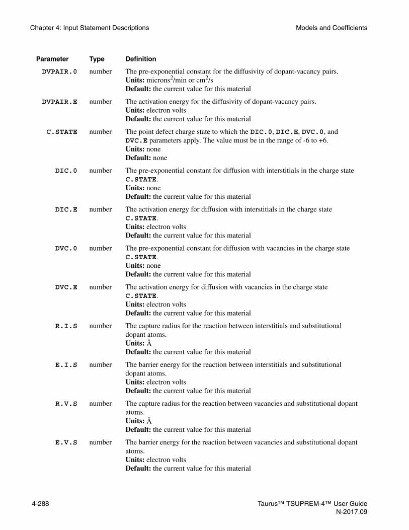
Chapter 4: Input Statement Descriptions Models and Coefficients

DVPAIR.0 number The pre-exponential constant for the diffusivity of dopant-vacancy pairs. Units: microns2/min or cm2/sDefault: the current value for this material

DVPAIR.E number The activation energy for the diffusivity of dopant-vacancy pairs.Units: electron volts Default: the current value for this material

C.STATE number The point defect charge state to which the DIC.0, DIC.E, DVC.0, and DVC.E parameters apply. The value must be in the range of -6 to +6.Units: noneDefault: none

DIC.0 number The pre-exponential constant for diffusion with interstitials in the charge state C.STATE.Units: none Default: the current value for this material

DIC.E number The activation energy for diffusion with interstitials in the charge state C.STATE.Units: electron volts Default: the current value for this material

DVC.0 number The pre-exponential constant for diffusion with vacancies in the charge state C.STATE.Units: none Default: the current value for this material

DVC.E number The activation energy for diffusion with vacancies in the charge state C.STATE.Units: electron volts Default: the current value for this material

R.I.S number The capture radius for the reaction between interstitials and substitutional dopant atoms.Units: ÅDefault: the current value for this material

E.I.S number The barrier energy for the reaction between interstitials and substitutional dopant atoms.Units: electron voltsDefault: the current value for this material

R.V.S number The capture radius for the reaction between vacancies and substitutional dopant atoms.Units: ÅDefault: the current value for this material

E.V.S number The barrier energy for the reaction between vacancies and substitutional dopant atoms.Units: electron voltsDefault: the current value for this material

Parameter Type Definition

4-288 Taurus™ TSUPREM-4™ User GuideN-2017.09

Models and Coefficients Chapter 4: Input Statement Descriptions

R.IP.V number The capture radius for the reaction between dopant-interstitial pairs and vacancies.Units: ÅDefault: the current value for this material

E.IP.V number The barrier energy for the reaction between dopant-interstitial pairs and vacancies.Units: electron voltsDefault: the current value for this material

R.VP.I number The capture radius for the reaction between dopant-vacancy pairs and interstitials.Units: ÅDefault: the current value for this material

E.VP.I number The barrier energy for the reaction between dopant-vacancy pairs and interstitials.Units: electron voltsDefault: the current value for this material

IP.V.LOW logical Assume that only dopant-interstitial pairs and vacancies having opposite charges of equal magnitude react in bulk material.Default: true

IP.V.MED logical Assumes that uncharged dopant-interstitial pairs (or vacancies) can react with vacancies (or dopant-interstitial pairs) in any charged state, and that oppositely charged dopant-interstitial pairs and vacancies can react.Default: false

IP.V.HIG logical Assumes that dopant-vacancy pairs in any charged state can react with interstitials in any charged state.Default: false

VP.I.LOW logical Assumes that only dopant-vacancy pairs and interstitials having opposite charges of equal magnitude react in bulk material.Default: true

VP.I.MED logical Assumes that uncharged dopant-vacancy pairs (or interstitials) can react with interstitials (or dopant-vacancy pairs) in any charged state, and that oppositely charged dopant-vacancy pairs and interstitials can react.Default: false

VP.I.HIG logical Assumes that dopant-vacancy pairs in any charged state can react with interstitials in any charged state.Default: false

EQ.FRACA logical Specifies to set the dopant-interstitial pair and dopant-vacancy pair concentrations to local equilibrium in crystalline regrowth region of silicon amorphized by implant damage.Default: false

Parameter Type Definition

Taurus™ TSUPREM-4™ User Guide 4-289N-2017.09

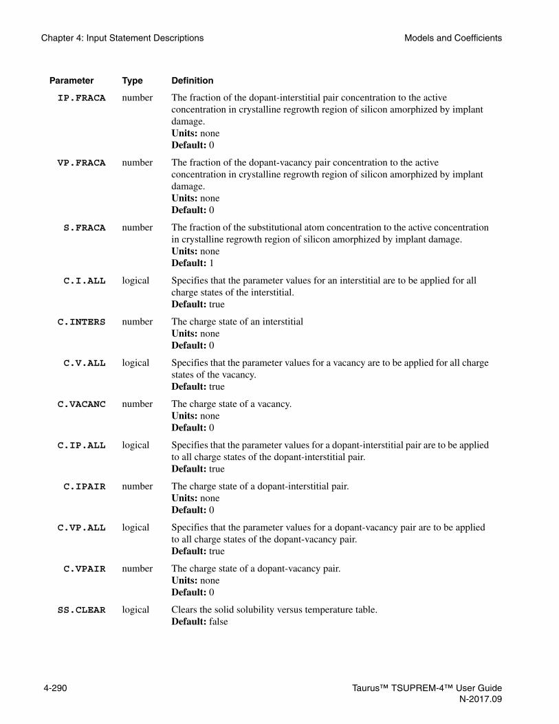
Chapter 4: Input Statement Descriptions Models and Coefficients

IP.FRACA number The fraction of the dopant-interstitial pair concentration to the active concentration in crystalline regrowth region of silicon amorphized by implant damage.Units: noneDefault: 0

VP.FRACA number The fraction of the dopant-vacancy pair concentration to the active concentration in crystalline regrowth region of silicon amorphized by implant damage.Units: noneDefault: 0

S.FRACA number The fraction of the substitutional atom concentration to the active concentration in crystalline regrowth region of silicon amorphized by implant damage.Units: noneDefault: 1

C.I.ALL logical Specifies that the parameter values for an interstitial are to be applied for all charge states of the interstitial.Default: true

C.INTERS number The charge state of an interstitialUnits: noneDefault: 0

C.V.ALL logical Specifies that the parameter values for a vacancy are to be applied for all charge states of the vacancy.Default: true

C.VACANC number The charge state of a vacancy.Units: noneDefault: 0

C.IP.ALL logical Specifies that the parameter values for a dopant-interstitial pair are to be applied to all charge states of the dopant-interstitial pair.Default: true

C.IPAIR number The charge state of a dopant-interstitial pair.Units: noneDefault: 0

C.VP.ALL logical Specifies that the parameter values for a dopant-vacancy pair are to be applied to all charge states of the dopant-vacancy pair.Default: true

C.VPAIR number The charge state of a dopant-vacancy pair.Units: noneDefault: 0

SS.CLEAR logical Clears the solid solubility versus temperature table. Default: false

Parameter Type Definition

4-290 Taurus™ TSUPREM-4™ User GuideN-2017.09

Models and Coefficients Chapter 4: Input Statement Descriptions

SS.TEMP number The temperature at which the solid solubility in the material is SS.CONC. Units: °Celsius Default: none

SS.CONC number The solid solubility in the material at temperature SS.TEMP. Units: atoms/cm3 Default: none

CTN.0 number The pre-exponential constant for impurity clustering. Units: (atoms/cm3)(1/CTN.F-1) Default: the current value for this material

CTN.E number The activation energy for impurity clustering. Units: electron volts Default: the current value for this material

CTN.F number The exponent of concentration for impurity clustering. Units: none Default: the current value for this material

CL.INI.A logical Specifies that impurities in an amorphized region are initially clustered when ACT.TRAN or ACT.FULL are used.Default: the current value for this impurity and material; initially true for built-in impurities in silicon

DDC.F.0 number The pre-exponential constant for dopant-interstitial clustering. Units: noneDefault: the current value for this material

DDC.F.E number The activation energy for dopant-interstitial clustering.Units: electron volts Default: the current value for this material

DDC.T.0 number The pre-exponential constant for the dopant-interstitial cluster dissolution time. Units: secondsDefault: the current value for this material

DDC.T.E number The activation energy for the dopant-interstitial cluster dissolution time.Units: electron volts Default: the current value for this material

DDCF.D.N number The power of the dopant concentration in the dopant-interstitial cluster formation reaction. Units: noneDefault: the current value for this material

DDCF.N.N number The power of the electron concentration in the dopant-interstitial cluster formation reaction.Units: noneDefault: the current value for this material

Parameter Type Definition

Taurus™ TSUPREM-4™ User Guide 4-291N-2017.09

Chapter 4: Input Statement Descriptions Models and Coefficients

DDCF.I.N number The power of the interstitial concentration in the dopant-interstitial cluster formation reaction.Units: noneDefault: the current value for this material

DDCR.N.N number The power of the electron concentration in the dopant-interstitial cluster dissolution reaction.Units: noneDefault: the current value for this material

DDCR.I.N number The power of the interstitial concentration in the dopant-interstitial cluster dissolution reaction.Units: noneDefault: the current value for this material

IFRACM number The number of interstitials per a dopant atom trapped in dopant-interstitial clusters.Units: noneDefault: the current value for this material

DDCS.0 number The pre-exponential constant for the dopant contained in small dopant-interstitial clusters at equilibrium. Units: noneDefault: the current value for this material

DDCS.E number The activation energy for the dopant contained in small dopant-interstitial clusters at equilibrium.Units: electron volts Default: the current value for this material

DDCS.N number The number of dopant atoms contained in each small dopant-interstitial cluster. Only values of 1 and 2 are meaningful, and only the value in silicon is used.Units: noneDefault: the current value for this material

IFRACS number The number of interstitials per dopant atom trapped in small dopant-interstitial clusters.Units: noneDefault: the current value for this material

DVC.F.0 number The pre-exponential constant for dopant-vacancy clustering. Units: noneDefault: the current value for this material

DVC.F.E number The activation energy for dopant-vacancy clustering.Units: electron volts Default: the current value for this material

DVC.T.0 number The pre-exponential constant for the dopant-vacancy cluster dissolution time. Units: secondsDefault: the current value for this material

Parameter Type Definition

4-292 Taurus™ TSUPREM-4™ User GuideN-2017.09

Models and Coefficients Chapter 4: Input Statement Descriptions

DVC.T.E number The activation energy for the dopant-vacancy cluster dissolution time.Units: electron volts Default: the current value for this material

DVCF.D.N number The power of the dopant concentration in the dopant-vacancy cluster formation reaction. Units: noneDefault: the current value for this material

DVCF.N.N number The power of the electron concentration in the dopant-vacancy cluster formation reaction.Units: noneDefault: the current value for this material

DVCF.V.N number The power of the interstitial concentration in the dopant-vacancy cluster formation reaction.Units: noneDefault: the current value for this material

DVCR.N.N number The power of the electron concentration in the dopant-vacancy cluster dissolution reaction.Units: noneDefault: the current value for this material

DVCR.V.N number The power of the interstitial concentration in the dopant-vacancy cluster dissolution reaction.Units: noneDefault: the current value for this material

VFRACM number The number of vacancies per a dopant atom trapped in dopant-vacancy clusters.Units: noneDefault: the current value for this material

C0.TF.0 number The prefactor in the expression for the activation time constant for the precipitation of this impurity in the ACT.FULL model.Units: secondsDefault: the current value for this impurity.

C0.TF.E number The activation energy in the expression for the activation time constant for the precipitation of this impurity in the ACT.FULL or DDC.FULL model.Units: electron voltsDefault: the current value for this impurity.

C0.TR.0 number The prefactor in the expression for the activation time constant for the dissolution of this impurity precipitation in the ACT.FULL or DDC.FULL model.Units: secondsDefault: the current value for this impurity.

Parameter Type Definition

Taurus™ TSUPREM-4™ User Guide 4-293N-2017.09

Chapter 4: Input Statement Descriptions Models and Coefficients

C0.TR.E number The activation energy in the expression for the activation time constant for the dissolution of this impurity precipitation in the ACT.FULL or DDC.FULL model.Units: electron voltsDefault: the current value for this impurity.

DDC.L character The solution name of the dopant-defect cluster in the left-hand side (reactant) of the reaction in the DDC.FULL model.Default: none

DDC.R character The solution name of the dopant-defect cluster in the right-hand side (product) of the reaction in the DDC.FULL model.Default: noneSynonym: DDCLUSTE

I.DDC logical Specifies that the dopant-defect cluster DDC.R is generated by the reaction with an silicon interstitial in the DDC.FULL model.Default: false

IP.DDC logical Specifies that the dopant-defect cluster DDC.R is generated by the reaction with a dopant-interstitial pair in the DDC.FULL model.Default: false

V.DDC logical Specifies that the dopant-defect cluster DDC.R is generated by the reaction with a vacancy in the DDC.FULL model.Default: false

VP.DDC logical Specifies that the dopant-defect cluster DDC.R is generated by the reaction with a dopant-vacancy pair in the DDC.FULL model.Default: false

DDC.KF.0 number The prefactor of the dopant-defect clustering forward reaction rate in the DDC.FULL model. Units: cm3/sDefault: the current value for this impurity

DDC.KF.E number The activation energy of the dopant-defect clustering forward reaction rate in the DDC.FULL model.Units: electron voltsDefault: the current value for this impurity

DDC.KR.0 number The prefactor of the dopant-defect clustering reverse reaction rate in the DDC.FULL model. Units: 1/sDefault: the current value for this impurity

DDC.KR.E number The activation energy of the dopant-defect clustering reverse reaction rate in the DDC.FULL model.Units: electron voltsDefault: the current value for this impurity

Parameter Type Definition

4-294 Taurus™ TSUPREM-4™ User GuideN-2017.09

Models and Coefficients Chapter 4: Input Statement Descriptions

DDC.EQ.0 number The prefactor of the equilibrium ratio of dopant-defect clustering reaction rate in the DDC.FULL model. Units: atoms/cm3 Default: the current value for this impurity

DDC.EQ.E number The activation energy of the equilibrium ratio of dopant-defect clustering reaction rate in the DDC.FULL model.Units: electron voltsDefault: the current value for this impurity

DDCFRACC number The fraction of DDC.R or DDC.L to the tot al dopant-defect clusters in a crystalline region after implants in the DDC.FULL model.Default: the current value for the dopant-defect cluster

DDCFRACA number The fraction of DDC.R or DDC.L to the total dopant-defect clusters in a recrystallized region after implants in the DDC.FULL model.Default: the current value for the dopant-defect cluster

DDC.C.IP number The charge state of the second dopant-interstitial pair for the reaction, , in the DDC.FULL model.

Units: noneDefault: 0

DDC.C.VP number The charge state of the second dopant-vacancy pair for the reaction, , in the DDC.FULL model.

Units: noneDefault: 0

DDCPRINT logical Specifies to print all dopant-defect clustering reactions and their reaction parameter values for this impurity in the DDC.FULL model.Default: false

C1FRAC.A number The fraction of dopant-interstitial cluster to the whole clusters, that is, dopant-interstitial clusters and precipitates upon implantation. Applies only inside of the amorphized regions whenever either ACT.FULL model or the DDC.FULL model is used. The value must be set in the range from 0.0 to 1.0.Units: noneDefault: 0

C2FRAC.A number The fraction of dopant-vacancy cluster to the whole clusters, that is, dopant-interstitial clusters and precipitates upon implantation. Applies only inside of the amorphized regions whenever either ACT.FULL model or the DDC.FULL model is used. The value must be set in the range from 0.0 to 1.0.Units: noneDefault: 0

C0.INI.F number The fraction of dopant in precipitation upon implantation. Applies only outside of the amorphized regions whenever either ACT.FULL model or DDC.FULL model is used. Inside the amorphized regions, ACT.AMOR value determines the activation level. The value must be set in the range from 0.0 to 1.0.Units: noneDefault: 0

Parameter Type Definition

XI XI+ X2I2↔

XV XV+ X2V2↔

Taurus™ TSUPREM-4™ User Guide 4-295N-2017.09

Chapter 4: Input Statement Descriptions Models and Coefficients

C1.INI.F number The fraction of dopant that is clustered upon implantation by the dopant-interstitial clustering model. Applies only outside of the amorphized regions whenever either ACT.FULL model or DDC.FULL model is used. Inside the amorphized regions, ACT.AMOR value determines the activation level. The value must be set in the range from 0.0 to 1.0.Units: noneDefault: 0Synonym: INI.DDC

C2.INI.F number The fraction of dopant that is clustered upon implantation by the dopant-vacancy clustering model. Applies only outside of the amorphized regions whenever either ACT.FULL model or DDC.FULL model is used. Inside the amorphized regions, ACT.AMOR value determines the activation level. The value must be set in the range from 0.0 to 1.0.Units: noneDefault: 0Synonym: INI.DDC

DDCTOT.C number The fraction of the total dopant-defect clusters including C1,C2 and all DDCs to the total dopants in a crystalline region after implants. Required when the DDC.FULL model is used or both C1 and C2 exist in the ACT.FULL model.Default: the current value for the dopant-defect cluster and the material

DDCTOT.A number The fraction of the total dopant-defect clusters to the total clusters in a recrystallized region after implants. Required when the DDC.FULL model is used or both C1 and C2 exist in the ACT.FULL model.Default: the current value for the dopant-defect cluster and the material

ACT.NI number The factor by which the intrinsic carrier concentration is multiplied to obtain the minimum activation level used by the ACT.FULL model for this impurity.Units: noneDefault: the current value for this impurity.

ACT.AMOR number The threshold concentration above which the dopant is inactive for the ACT.FULL dopant activation model at the beginning of the post-implant anneal. Applies only inside the amorphized regions. Outside of the amorphized regions - see C0.INI.F, C1.INI.F parameters.Units: cm-3 Default: the current value for this impurity

ACT.INSI number The threshold concentration above which the dopant added at each incremental layer for deposition and epitaxy is inactive.Units: cm-3 Default: the current value for this impurity

MAX.AMOR number Maximum impurity concentration that can survive epitaxial recrystallization of the amorphized layer. Everything above this concentration is swept by the advancing recrystallization front.Units: cm-3 Default: 6e18 for indium and 5e22 for the other impuritiesSynonym: MAX.SPE

Parameter Type Definition

4-296 Taurus™ TSUPREM-4™ User GuideN-2017.09

Models and Coefficients Chapter 4: Input Statement Descriptions

FGB number The factor by which the diffusivity is increased in polycrystalline materials when the polycrystalline model is not enabled.Units: none Default: the current value for this material

Q.SITES number The density of dopant sites in grain boundaries (the maximum allowable value for the grain-boundary concentration) in a polycrystalline material.Units: #/cm2

Default: the current value for this material

CG.MAX number The density of dopant sites in the grain interior of a polycrystalline material.Units: #/cm3

Default: the current value for this material; initially 5e22 for polysilicon

GSEG.0 number The entropy for segregation between grain interior and boundaries in a polycrystalline material.Units: noneDefault: the current value for this material Synonym: A.SEG

GSEG.E number The activation energy of the segregation entropy between grain interior and boundaries in a polycrystalline material.Units: electron voltsDefault: the current value for this material Synonym: E.SEG

GSEG.INI number The entropy for the initial segregation between grain interior and boundaries in a polycrystalline material.Units: noneDefault: the current value for this material Synonym: A0.SEG

FVELB.0 number The pre-exponential factor of the multiplication factor to the segregation velocity in the grain interiors of a polycrystalline material.Units: noneDefault: the current value for this material

FVELB.E number The activation energy of the multiplication factor to the segregation velocity in the grain interiors of a polycrystalline material.Units: electron voltsDefault: the current value for this material

VELIF.0 number The pre-exponential factor for the segregation velocity at the boundaries of a polycrystalline material.Units: cm/sDefault: the current value for this material

VELIF.E number The activation energy for the segregation velocity at the boundaries of a polycrystalline material.Units: electron voltsDefault: the current value for this material

Parameter Type Definition

Taurus™ TSUPREM-4™ User Guide 4-297N-2017.09

Chapter 4: Input Statement Descriptions Models and Coefficients

MODEL character The name of the model to which the diffusion equations for the new impurity are registered. The ENABLE parameter, with the MODEL parameter given by this name in the METHOD statement, specifies the diffusion equation for this impurity to be solved.Default: noneSynonym: D.MODEL

EQACTIVE character The expression of calculation for the equilibrium active concentration of the dopant. The equilibrium active concentration of the dopant in the given material is to be calculated by the EQACTIVE expression instead of calling the built-in function.Default: none

ACTIVE character The expression of calculation for the active concentration of the dopant. The active concentration of the dopant in the given material is to be calculated by the ACTIVE expression instead of calling the built-in function.Default: none

MOBILE character The expression of calculation for the mobile concentration of the dopant. The mobile concentration of the dopant in the given material is to be calculated by the MOBILE expression instead of calling the built-in function.Default: none

DI.FAC character The expression of multiplication factor to the diffusion with interstitials.Default: “1.0”

DV.FAC character The expression of multiplication factor to the diffusion with vacancies.Default: “1.0”

DI.F11 character The expression of multiplication factor to the horizontal diffusion with interstitials.Default: “1.0”

DI.F22 character The expression of multiplication factor to the vertical diffusion with interstitials.Default: “1.0”

DV.F11 character The expression of multiplication factor to the horizontal diffusion with vacancies.Default: “1.0”

DV.F22 character The expression of multiplication factor to the vertical diffusion with vacancies.Default: “1.0”

/MATERIA character The name of material 2 for the segregation and transport parameters.Default: none

SEG.0 number The pre-exponential factor for segregation from material 1 to material 2.For the trapped impurity at interface, the pre-exponential factor for segregation from material 1 to interface adjacent to material 2.Units: none for the segregation from material 1 to material 2, cm-1 for the segregation from material 1 to interfaceDefault: the current value for these materials

Parameter Type Definition

4-298 Taurus™ TSUPREM-4™ User GuideN-2017.09

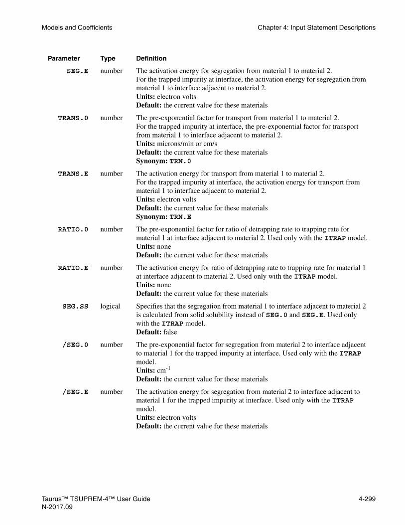
Models and Coefficients Chapter 4: Input Statement Descriptions

SEG.E number The activation energy for segregation from material 1 to material 2. For the trapped impurity at interface, the activation energy for segregation from material 1 to interface adjacent to material 2.Units: electron volts Default: the current value for these materials

TRANS.0 number The pre-exponential factor for transport from material 1 to material 2.For the trapped impurity at interface, the pre-exponential factor for transport from material 1 to interface adjacent to material 2.Units: microns/min or cm/s Default: the current value for these materialsSynonym: TRN.0

TRANS.E number The activation energy for transport from material 1 to material 2. For the trapped impurity at interface, the activation energy for transport from material 1 to interface adjacent to material 2.Units: electron volts Default: the current value for these materialsSynonym: TRN.E

RATIO.0 number The pre-exponential factor for ratio of detrapping rate to trapping rate for material 1 at interface adjacent to material 2. Used only with the ITRAP model.Units: noneDefault: the current value for these materials

RATIO.E number The activation energy for ratio of detrapping rate to trapping rate for material 1 at interface adjacent to material 2. Used only with the ITRAP model.Units: noneDefault: the current value for these materials

SEG.SS logical Specifies that the segregation from material 1 to interface adjacent to material 2 is calculated from solid solubility instead of SEG.0 and SEG.E. Used only with the ITRAP model.Default: false

/SEG.0 number The pre-exponential factor for segregation from material 2 to interface adjacent to material 1 for the trapped impurity at interface. Used only with the ITRAP model.Units: cm-1

Default: the current value for these materials

/SEG.E number The activation energy for segregation from material 2 to interface adjacent to material 1 for the trapped impurity at interface. Used only with the ITRAP model.Units: electron volts Default: the current value for these materials

Parameter Type Definition

Taurus™ TSUPREM-4™ User Guide 4-299N-2017.09

Chapter 4: Input Statement Descriptions Models and Coefficients

/TRANS.0 number The pre-exponential factor for transport from material 2 to interface adjacent to material 1 for the trapped impurity at interface. Used only with the ITRAP model.Units: microns/min or cm/s Default: the current value for these materialsSynonym: /TRN.0

/TRANS.E number The activation energy for transport from material 2 to interface adjacent to material 1 for the trapped impurity at interface. Used only with the ITRAP model.Units: electron volts Default: the current value for these materialsSynonym: /TRN.E

/RATIO.0 number The pre-exponential factor for ratio of detrapping rate to trapping rate for material 2 at interface adjacent to material 1. Used only with the ITRAP model.Units: noneDefault: the current value for these materials

/RATIO.E number The activation energy for ratio of detrapping rate to trapping rate for material 2 at interface adjacent to material 1. Used only with the ITRAP model.Units: noneDefault: the current value for these materials

/SEG.SS logical Specifies that the segregation from material 2 to interface adjacent to material 1 is calculated from solid solubility instead of /SEG.0 and /SEG.E. Used only with the ITRAP model.Default: false

SEG.EQ3 logical Specifies that both of segregations from material 1 to interface and from material 2 to interface are determined from the values of the parameters, SEG.0, SEG.E, /SEG.0 and /SEG.E. Used only with the ITRAP model.Default: true

SEG.EQ2 logical Specifies that the segregation from material 1 to interface is determined to make the concentration ratio in materials 1 and 2 in 3-phase equilibrium equal to the one in 2-phase equilibrium. Used only with the ITRAP model.Default: false

/SEG.EQ2 logical Specifies that the segregation from material 2 to interface is determined to make the concentration ratio in materials 1 and 2 in 3-phase equilibrium equal to the one in 2-phase equilibrium. Used only with the ITRAP model.Default: false

Q.INI.0 number The pre-exponential factor for the initial occupied trap density at interface. Used only with the ITRAP model.Units: atoms/cm2

Default: the current value for these materials

Parameter Type Definition

4-300 Taurus™ TSUPREM-4™ User GuideN-2017.09

Models and Coefficients Chapter 4: Input Statement Descriptions

Q.INI.E number The activation energy for the initial occupied trap density at interface. Used only with the ITRAP model.Units: electron volts Default: the current value for these materials

Q.MAX.0 number The pre-exponential factor for the maximum trap density at interface. Used only with the ITRAP model.Units: atoms/cm2

Default: the current value for these materials

Q.MAX.E number The activation energy for the maximum trap density at interface. Used only with the ITRAP model.Units: electron volts Default: the current value for these materials

TWO.PHAS logical Specifies that the flux of 2-phase segregation is added to the one of 3-phase segregation flux. Used only with the ITRAP model.Default: false

KSIP.0 number The pre-exponential constant for the surface recombination velocity of the dopant-interstitial pair at the interface between the specified materials.Units: microns/min or cm/sDefault: the current value for these materials

KSIP.E number The activation energy for the surface recombination velocity of the dopant-interstitial pair at the interface between the specified materialsUnits: electron voltsDefault: the current value for these materials

KSVP.0 number The pre-exponential constant for the surface recombination velocity of the dopant-vacancy pair at the interface between the specified materials.Units: microns/min or cm/sDefault: the current value for these materials

KSVP.E number The activation energy for the surface recombination velocity of the dopant-vacancy pair at the interface between the specified materialsUnits: electron voltsDefault: the current value for these materials

SEG.IFRA number The fraction of a dopant-interstitial pairing to the dopant-defect pairing for pair segregation model. The value must be >= 0 and <= 1.0. Only applicable when the PAIR.SEG parameter is turned on in the METHOD statement.Units: noneDefault: the current value for these materials

SEG.IPOW number The power of interstitial concentration to which the segregation transport rate is proportional. The parameter value physically means the number of interstitials to be generated or recombined during segregation. Only applicable when the PAIR.SEG parameter is turned on in the METHOD statement.Units: noneDefault: the current value for these materials

Parameter Type Definition

Taurus™ TSUPREM-4™ User Guide 4-301N-2017.09

Chapter 4: Input Statement Descriptions Models and Coefficients

SEG.VPOW number The power of vacancy concentration to which the segregation transport rate is proportional. The parameter value physically means the number of vacancies to be generated or recombined during segregation. Only applicable when the PAIR.SEG parameter is turned on in the METHOD statement.Units: noneDefault: the current value for these materials

SEG.CPOW number The power of n/ni in the Fermi-level dependent segregation model. The parameter value physically means the number of charge carriers to be generated or annihilated during segregation.Units: noneDefault: the current value for these materials

ES.RAND number The electronic stopping power coefficient of implanted atoms in the specified material for materials other than silicon and for a nonchanneled direction in silicon. This value is used for the MC ion implant calculation only.Units: angstrom2*eV(1-ES.F.RAN) Default: the current value for the specified materials

ES.F.RAN number The exponent of the electronic stopping power of implanted atoms in the specified material for materials other than silicon and for a nonchanneled direction in silicon. This value is used for the MC ion implant calculation only.Units: none Default: the current value for the specified materials

ES.BREAK number The energy above which ES.F.H is used, instead of ES.F.RAN, ES.F.100, or ES.F.110, in calculating the electronic stopping power coefficient of implanted atoms. This value is used for the MC ion implant calculation only.Units: keV Default: the current value for the specified materials

ES.F.H number The exponent of the electronic stopping power of implanted atoms at energies above ES.BREAK. This value is used for the MC ion implant calculation only.Units: none Default: the current value for the specified materials

ES.100 number The electronic stopping power for implanted atoms in silicon along the <100> channeling axes. This value is used for the MC ion implant calculation only.Units: angstrom2*eV(1-ES.F.100) Default: the current value for the specified materials

ES.F.100 number The exponent of the electronic stopping power for implanted atoms in silicon along the <100> crystal axes. This value is used for the MC ion implant calculation only.Units: none Default: the current value for the specified material

ES.110 number The electronic stopping power for implanted atoms in silicon along the <110> channeling axes. This value is used for the MC ion implant calculation only.Units: angstrom2*eV(1-ES.F.100) Default: the current value for the specified material

Parameter Type Definition

4-302 Taurus™ TSUPREM-4™ User GuideN-2017.09

Models and Coefficients Chapter 4: Input Statement Descriptions

ES.F.110 number The exponent of the electronic stopping power for implanted atoms in silicon along the <110> crystal axes. This value is used for the MC ion implant calculation only.Units: none Default: the current value for the specified material

NLOC.PRO number The prefactor for the nonlocal electronic stopping power formula. This value is used for the OLD.MC ion implant calculation only.Units: noneDefault: 0.3

NLOC.EXO number The exponent for the nonlocal electronic stopping power formula. This value is used for the OLD.MC ion implant calculation only.Units: noneDefault: 0.2

NLOC.MAX number The maximum value allowed for the nonlocal part of electronic stopping power. This value is used for the OLD.MC ion implant calculation only.Units: noneDefault: 0.6

NLOC.K number A correction factor for the LSS electron stopping power. This value is used for the OLD.MC ion implant calculation only.Units: noneDefault: 1.2

LOC.FAC number A correction factor for the local part of electronic stopping power. This value is sued for the OLD.MC ion implant calculation only.Units: noneDefault: 0.8

CHAN.CRI number Specifies the critical angle below which the scattering angle is automatically reduced. This value is used for the OLD.MC ion implant calculation only.Units: noneDefault: 11.54

CHAN.FAC number Specifies the factor by which the scattering angle is reduced. This value is used for the OLD.MC ion implant calculation only.Units: noneDefault: 2.0

DISP.FAC number This is a correction factor for the probability of selecting the amorphous model. This value is used for the OLD.MC ion implant calculation only.Units: noneDefault: 0.5

DIV.ANG number Angular divergence angle of ion beam. This parameter is used for Taurus MC only.Units: degreeDefault: 0.5

Parameter Type Definition

Taurus™ TSUPREM-4™ User Guide 4-303N-2017.09

Chapter 4: Input Statement Descriptions Models and Coefficients

REC.FRAC number Fraction of secondary recoils to be traced for CASCADE damage model. For better accuracy, 1.0 should be used. Units: noneDefault: 1.0

LSS.PRE number A correction factor for the LSS electron stopping power. This parameter is used for Taurus MC only.Units: noneDefault: 1.0

NLOC.PRE number The prefactor for the nonlocal electronic stopping power formula. This parameter is used for Taurus MC only.Units: noneDefault: 0.5

NLOC.EXP number The exponent for the nonlocal electronic stopping power formula. This parameter is used for Taurus MC only.Units: noneDefault: 0.5

SCR.PAR number Adjustable parameter for screening length of local electronic stopping power.Units: noneDefault: 1.0

SURV.RAT number Survival rate of Frenkel pairs generated by the ion beam for the default PLUS damage model. This parameter is used for Taurus MC only.Units: noneDefault: 1.0

AMOR.PAR number Proportional factor for the switching probability from crystalline to amorphous model for the default PLUS damage model. This parameter is used for Taurus MC only.Units: noneDefault: 1.0

DISP.THR number Displacement threshold for the default PLUS damage model. This parameter is used for Taurus MC only.Units: eVDefault: 15

SAT.PAR number Damage saturation parameter for MC implant.The saturation value is equal to (lattice density)/SAT.PAR. This parameter is used for Taurus MC only.Units: noneDefault: 1.0

CASC.SUR number Survival rate of Frenkel pairs generated by the ion beam for CASCADE damage model. This parameter is used for Taurus MC only.Units: noneDefault: 1.0

Parameter Type Definition

4-304 Taurus™ TSUPREM-4™ User GuideN-2017.09

Models and Coefficients Chapter 4: Input Statement Descriptions

Description This statement is used to define new impurities and specify their properties. If NEW is specified, a new impurity is defined; otherwise the properties of an existing impurity are set.

The coefficients for standard impurities are given in the s4init file (which is read at the start of each TSUPREM-4 execution), but you can change these at any time. Coefficients that are not given in the s4init file or set by the user, default to 0.0, except for SEG.0, which defaults to 1.0.

Parameters whose units include time are specified in units of microns and minutes, unless CM.SEC is true, in which case units of centimeters and seconds are assumed.

The IMPURITY statement replaces the ANTIMONY, ARSENIC, BORON, and PHOSPHORUS statements; the old statements are still available, however, for compatibility with existing input files.

For additional information, see the following sections:

• Use of the diffusion parameters, Chapter 3, Diffusion of Impurities, p. 3-18.

• Solid solubility and clustering parameters, Chapter 3, Activation of Impurities, p. 3-35.

• Segregation parameters, Chapter 3, Activation of Impurities, p. 3-35.

• Electronic stopping power parameters, Chapter 3, MC Ion Implant Model, p. 3-147.

Impurity Type DONOR and ACCEPTOR specify whether the impurity is a donor or an acceptor. By default, newly defined impurities are electrically inactive. Once they have been specified to be active (with the DONOR or ACCEPTOR parameters), they cannot be returned to their electrically inactive state.

CASC.AMO number Proportional factor for the switching probability from crystalline to amorphous model for the CASCADE damage model. This parameter is used for Taurus MC only.Units: noneDefault: 1.0

CASC.DIS number Displacement threshold for CASCADE damage model. This parameter is used for Taurus MC only.Units: eVDefault: 15

CASC.SAT number Damage saturation parameter for cascade damage model. The saturation value is equal to (lattice density)/CASC.SAT. This parameter is used for Taurus MC only.Units: noneDefault: 1.0

Parameter Type Definition

Taurus™ TSUPREM-4™ User Guide 4-305N-2017.09

Chapter 4: Input Statement Descriptions Models and Coefficients

Solution Options SOLVE specifies whether diffusion equations are solved for this impurity; if SOLVE is false, the impurity is assumed to be immobile. If the MODEL name is given, turning off the given model in METHOD statement is the same as turning off SOLVE in IMPURITY statement. Turning off DIFFUSE parameter specifies that the diffusion equation is not solved for this impurity in the specified material. STEADY specifies whether a steady-state or full transient solution to the diffusion equations should be computed. The steady-state solution is preferred for impurities that diffuse rapidly or react at material interfaces to produce material growth or consumption. The full transient solution is preferred for impurities that diffuse slowly or interact with other impurities.

OtherParameters

AT.NUM and AT.WT are used by the MC implantation model. IMPL.TAB specifies the name of the implant moment table to be used for the impurity.

The initial background concentration of a user-defined impurity when it is first added to a structure is given by C.INIT. For normal impurities, C.INIT should be greater than zero; a value of 1e5 (the value used for built-in impurities) is suggested.

Multiplication toDiffusivity

DI.FAC and DV.FAC describe the formulas for multiplication factors to diffusivities. D.MODEL names the DI.FAC and/or DV.FAC so that its application can be turned on or off. For example

IMPURITY IMP=BORON MAT=OXIDE MODEL=myDiff +DI.FAC=1+1e-21*fluorine

METHOD MODEL=myDiff !ENABLE

AnisotropicDiffusivity

DI.F11, DI.F22, DV.F11 and DV.FAC describe the formulas for multiplication factors to anisotropic diffusivities. For example,:

INTERMED NAME=qkT EXPR=1E31*KB*TEMPINTERMED NAME=SD11 EXPR=exp(Sxx*15.73/qkT)INTERMED NAME=SD22 EXPR=exp(Syy*15.73/qkT)IMPURITY MODEL=AnisoSD IMP=BORON MAT=Si +

DI.F11=SD11 DV.F11=SD11 DI.F22=SD22 DV.F22=SD22

SD11 and SD22 assigned to DI.F11, DI.F22, DV.F11, and DV.F22 can be replaced with their expressions. However, using the intermediates reduces the calculation time when the same expressions are used in several places. Specifying the MODEL parameter is optional. It is useful to turn on/off the expressions by the METHOD statement.

For example, the above model can be turned off by;

METHOD MODEL=AnisoSD ^ENABLE

User-DefinedActive

Concentration

By setting an expression to the ACTIVE parameter in the IMPURITY command, you can change the function to calculate the dopant-active concentration in the transient state. The parameter EQACTIVE in the IMPURITY command defines the expression to calculate the equilibrium active concentration. Calling the

4-306 Taurus™ TSUPREM-4™ User GuideN-2017.09

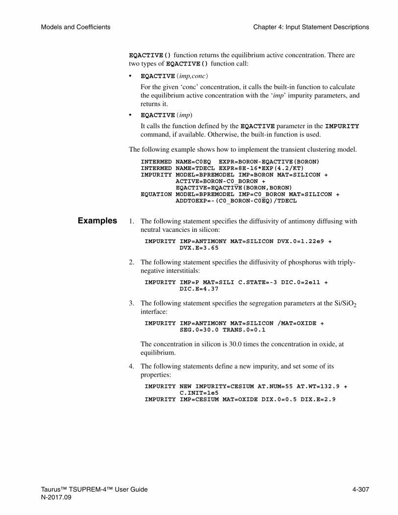
Models and Coefficients Chapter 4: Input Statement Descriptions

EQACTIVE() function returns the equilibrium active concentration. There are two types of EQACTIVE() function call:

• EQACTIVE(imp,conc)

For the given ‘conc’ concentration, it calls the built-in function to calculate the equilibrium active concentration with the ‘imp’ impurity parameters, and returns it.

• EQACTIVE(imp)

It calls the function defined by the EQACTIVE parameter in the IMPURITY command, if available. Otherwise, the built-in function is used.

The following example shows how to implement the transient clustering model.

INTERMED NAME=C0EQ EXPR=BORON-EQACTIVE(BORON)INTERMED NAME=TDECL EXPR=8E-16*EXP(4.2/KT)IMPURITY MODEL=BPREMODEL IMP=BORON MAT=SILICON +

ACTIVE=BORON-C0_BORON +EQACTIVE=EQACTIVE(BORON,BORON)

EQUATION MODEL=BPREMODEL IMP=C0_BORON MAT=SILICON +ADDTOEXP=-(C0_BORON-C0EQ)/TDECL

Examples 1. The following statement specifies the diffusivity of antimony diffusing with neutral vacancies in silicon:

IMPURITY IMP=ANTIMONY MAT=SILICON DVX.0=1.22e9 +DVX.E=3.65

2. The following statement specifies the diffusivity of phosphorus with triply-negative interstitials:

IMPURITY IMP=P MAT=SILI C.STATE=-3 DIC.0=2e11 +DIC.E=4.37

3. The following statement specifies the segregation parameters at the Si/SiO2 interface:

IMPURITY IMP=ANTIMONY MAT=SILICON /MAT=OXIDE +SEG.0=30.0 TRANS.0=0.1

The concentration in silicon is 30.0 times the concentration in oxide, at equilibrium.

4. The following statements define a new impurity, and set some of its properties:

IMPURITY NEW IMPURITY=CESIUM AT.NUM=55 AT.WT=132.9 +C.INIT=1e5

IMPURITY IMP=CESIUM MAT=OXIDE DIX.0=0.5 DIX.E=2.9

Taurus™ TSUPREM-4™ User Guide 4-307N-2017.09

Chapter 4: Input Statement Descriptions Models and Coefficients

REACTION

The REACTION statement defines the reactions that occur at material interfaces.

REACTION

{ MAT.BULK=<c> | ( MAT.R=<c> /MAT.L=<c> ) }[MODEL=<c>] [NAME=<c>] [ { DELETE | REPLACE } ]

{ ( [IMP.L=<c>] [NI.L=<n>] [EI.L=<n> ] [/IMP.L=<c>] [/NI.L=<n>] [/EI.L=<n> ] [IMP.R=<c>] [NI.R=<n>] [EI.R=<n> ] [/IMP.R=<c>] [/NI.R=<n>] [/EI.R=<n> ] [NM.R=<n>] [/NM.L=<n>] [RATE.0=<n>] [RATE.E=<n>] [R.FAC=<c>] [/R.FAC=<c>]

[EQUIL.0=<n>] [EQUIL.E=<n>] [E.FAC=<c>] [/E.FAC=<c>] ) | ( MAT.NEW=<c> THICKNES=<n> ) }

Parameter Type Definition

MAT.BULK character A name of bulk material, in which the reaction equation is applied.Default: none

MAT.R character Material 1, which appears on the right side of the reaction equation.Default: noneSynonyms: MAT, MAT1

/MAT.L character Material 2, which appears on the left side of the reaction equation.Default: noneSynonym: MAT2

MODEL character A name used to refer to this reaction. By turning on/off the ENABLE parameter with the MODEL parameter in the METHOD statement, the reaction can be enabled or disabled.Default: none

NAME character A name used to refer to this reaction in subsequent REACTION statements.Default: “<none>”

DELETE logical Deletes the specified reaction.Default: false

REPLACE logical Replaces the specified reaction.Default: false

IMP.L character The impurity in material 1 that appears on the left side of the reaction equation.Default: none

NI.L number The number of molecules of IMP.L that participate in the reaction.Units: noneDefault: 1.0

4-308 Taurus™ TSUPREM-4™ User GuideN-2017.09

Models and Coefficients Chapter 4: Input Statement Descriptions

EI.L number The exponent describing the dependence of the forward reaction rate on the concentration of IMP.L.Units: noneDefault: NI.L

/IMP.L character The impurity in material 2 that appears on the left side of the reaction equation.Default: none

/NI.L number The number of molecules of /IMP.L that participate in the reaction.Units: noneDefault: 1.0

/EI.L number The exponent describing the dependence of the forward reaction rate on the concentration of /IMP.L.Units: noneDefault: /NI.L

IMP.R character The impurity in material 1 that appears on the right side of the reaction equation.Default: none

NI.R number The number of molecules of IMP.R that participate in the reaction.Units: noneDefault: 1.0

EI.R number The exponent describing the dependence of the reverse reaction rate on the concentration of IMP.R.Units: noneDefault: NI.R

/IMP.R character The impurity in material 2 that appears on the right side of the reaction equation.Default: none

/NI.R number The number of molecules of /IMP.R that participate in the reaction.Units: noneDefault: 1.0

/EI.R number The exponent describing the dependence of the reverse reaction rate on the concentration of /IMP.R.Units: noneDefault: /NI.R

NM.R number The number of molecules of MAT.R that participate in the reaction.Units: noneDefault: 0.0

/NM.L number The number of molecules of /MAT.L that participate in the reaction.Units: noneDefault: 0.0

RATE.0 number The prefactor in the expression for the forward reaction rate.Units: variesDefault: 0.0

Parameter Type Definition

Taurus™ TSUPREM-4™ User Guide 4-309N-2017.09

Chapter 4: Input Statement Descriptions Models and Coefficients

Description The REACTION statement can specify either a reaction that takes place at the interface between two materials or the addition of a native layer when one material is deposited on another. Each reaction is identified by its name and the materials on either side of the interface. The name is optional: if no name is specified, the name “<none>” is assumed.

RATE.E number The activation energy for the forward reaction rate.Units: noneDefault: 0.0

R.FAC character A formula using solution variables defined in MAT.R, that multiplies the forward reaction rate.Units: noneDefault: 1.0

/R.FAC character A formula using solution variables defined in /MAT.L, that multiplies the forward reaction rate.Units: noneDefault: 1.0

EQUIL.0 number The prefactor in the expression for the ratio of the reverse reaction rate to the forward reaction rate.Units: variesDefault: 0.0

EQUIL.E number The activation energy for the ratio of the reverse reaction rate to the forward reaction rate.Units: noneDefault: 0.0

E.FAC character A formula using solution variables defined in MAT.R, that multiplies the ratio of the reverse reaction rate to the forward reaction rate.Units: noneDefault: 1.0

/E.FAC character A formula using solution variables defined in /MAT.L, that multiplies the ratio of the reverse reaction rate to the forward reaction rate.Units: noneDefault: 1.0

MAT.NEW character The name of the material to be added between layers of MAT.R and /MAT.L, when one is deposited on the other.Default: none

THICKNES number The thickness of MAT.NEW to be added between layers of MAT.R and /MAT.L, when one is deposited on the other. Units: micronsDefault: none

Parameter Type Definition

4-310 Taurus™ TSUPREM-4™ User GuideN-2017.09

Models and Coefficients Chapter 4: Input Statement Descriptions

Reactions defined with the REACTION statement take place during DIFFUSION steps with either oxidizing or inert ambients. The reactions occur only when the VERTICAL, COMPRESS, or VISCOELA oxidation model has been selected.

Defining andDeleting

A new reaction is defined by specifying a name (optional), the materials on either side of the interface, and the impurity and reaction rate parameters. The parameters for a previously defined reaction can be changed by specifying the name and materials for the reaction along with any parameters that need to be changed. A previously defined reaction can be deleted with the DELETE parameter. The REPLACE parameter deletes a previously defined reaction then replaces it with a new reaction defined by the parameters on the REACTION statement.

Insertion ofNative Layers

The MAT.NEW and THICKNES parameters specify a new material to be inserted between MAT.R and /MAT.L when one is deposited on the other. A layer of MAT.NEW with thickness THICKNES separates MAT.R and /MAT.L. The process is analogous to the insertion of a native oxide layer between exposed silicon and an oxidizing ambient.

ReactionEquation

The general form of the reaction is:

Equation 4-5

where the subscripts and denote terms on the left and right sides of the reaction, and subscripts 1 and 2 refer to materials 1 and 2. The forward and reverse reaction rates are given by:

Equation 4-6

Equation 4-7

where denotes the concentration of impurity .

Parameters Specify the parameters of this reaction as follows:

Equation 4-8

Equation 4-9

Equation 4-10

Equation 4-11

→nil1Il1 n+ il2Il2 nml2Ml2+ nmr1Mr1 nir1Ir1 nir2Ir2+ +←

l r

Rf kf Il1[ ]el1 Il2[ ]

el2=

Rr kr Ir1[ ]er1 Ir2[ ]

er2=

Ix[ ] Ix

Il1 IMP.L, Il2 IMP.L⁄ , Ir1 IMP.R, Ir2 IMP.R⁄====

nil1 NI.L, nil2 NI.L⁄ , nir1 NI.R, Iir2 NI.R⁄====

nmr1 NM.R, nml2 NM.L⁄==

eil1 EI.L, eil2 EI.L⁄ , eir1 EI.R, eir2 EI.R⁄====

Taurus™ TSUPREM-4™ User Guide 4-311N-2017.09

Chapter 4: Input Statement Descriptions Models and Coefficients

Equation 4-12

Equation 4-13

• NI.L, /NI.L, NI.R, /NI.R, NM.R, and /NM.L determine the number of molecules of each reactant that participate in the reaction.

• EI.L, /EI.L, EI.R, /EI.R, RATE.0, RATE.E, R.FAC, /R.FAC, EQUIL.0, EQUIL.E, E.FAC, and /E.FAC determine the rate of the reaction.

In theory, the and for each reaction would be equal, but this is not required by TSUPREM-4. This allows the rate to depend on the concentration of an impurity without the concentration being affected by the reaction ( ), or for the concentration to change without affecting the rate ( ).

The units of and are #/cm2/s; the units of and depend on the values of the and .

Effects This reaction has two effects on the simulation:

1. As a boundary condition for diffusing species, it can result in generation, consumption, or transport of impurities across a material interface. The impurity generation fluxes ( , in #/cm2/s) at the interface are given by

Equation 4-14

(Note that when is zero, the corresponding flux is also zero.)

2. It can produce growth or consumption of material regions. This occurs for materials for which . The growth rate of , in cm/s, is given by:

Equation 4-15

where is the growth velocity in cm/s, is Avogadro’s number, and MOL.WT and DENSITY are material parameters specified on the MATERIAL statement. The material is consumed ( ) if .

kf RATE.0= exp RATE.E–kT

----------------------- R.FAC /R.FAC⋅ ⋅ ⋅

kr

kf----

Il1[ ]el1 Il2[ ]

el2

Ir1[ ]er1 Ir2[ ]

er2--------------------------------- EQUIL.0 exp EQUIL.E–

kT-------------------------- E.FAC /E.FAC⋅ ⋅ ⋅= =

ni ei

ei 0 ni,≠ 0=

ei 0 ni 0≠,=

Rf Rr kf kr

ni ei

F

1

nil1--------Fl1–

1nil12----------Fl2–

1nir1---------Fr1

1nir2---------Fr2 Rf Rr–= = = =

ni

nm 0≠ Mrl

Vnmr1 MOL.WT×A DENSITY×

------------------------------------- Rf Rr–( )=

V A 6.022 1023×=

V 0< Rf Rr<

4-312 Taurus™ TSUPREM-4™ User GuideN-2017.09

Models and Coefficients Chapter 4: Input Statement Descriptions

MOBILITY

The MOBILITY statement is used to define or modify the dependence of carrier mobility on impurity concentration and temperature within a semiconductor.

MOBILITY

[ {TAB.TEMP=<n> [KELVIN] TAB.CONC=<c> TAB.E.MU=<c> TAB.H.MU=<c> [TAB.CLEA]} ] [ECN.MU=<n>] [ECP.MU=<n>] [GSURFN=<n>] [GSURFP=<n>] [MUN1=<n>] [MUN2=<n>] [AN=<n>] [CN=<n>] [EXN1=<n>] [EXN2=<n>] [EXN3=<n>] [EXN4=<n>] [MUP1=<n>] [MUP2=<n>] [AP=<n>] [CP=<n>] [EXP1=<n>] [EXP2=<n>] [EXP3=<n>] [EXP4=<n>] [MUN.MIN=<n>] [MUN.MAX=<n>] [NREFN=<n>] [NUN=<n>] [XIN=<n>] [ALPHAN=<n>] [MUP.MIN=<n>] [MUP.MAX=<n>] [NREFP=<n>] [NUP=<n>] [XIP=<n>] [ALPHAP=<n>]

Parameter Type Definition

TAB.TEMP number The temperature at which the mobility table values were measured. Units: Kelvins if the KELVIN parameter is specified, otherwise, degrees CelsiusDefault: none

KELVIN logical Specifies that the units of TAB.TEMP is Kelvins. Default: false

TAB.CONC character This parameter is interpreted as a series of numeric values, separated by spaces or commas. The parameter defines the concentrations associated with the mobilities defined in TAB.E.MU or TAB.H.MU.Units: atoms/cm3 Default: none

TAB.E.MU character This parameter is interpreted as a series of numeric values, separated by spaces or commas. The parameter defines the electron mobilities associated with the concentrations defined in TAB.CONC.Units: cm2/V/sDefault: none

TAB.H.MU character This parameter is interpreted as a series of numeric values, separated by spaces or commas. The parameter defines the hole mobilities associated with the concentrations defined in TAB.CONC.Units: cm2/V/sDefault: none

TAB.CLEA logical Specifies that the current table is to be cleared.Default: false

Taurus™ TSUPREM-4™ User Guide 4-313N-2017.09

Chapter 4: Input Statement Descriptions Models and Coefficients

ECN.MU number The critical electric field used to calculate the electron mobility degradation by perpendicular electric field.Units: V/cmDefault: 6.49e4

ECP.MU number The critical electric field used to calculate the hole mobility degradation by perpendicular electric field.Units: V/cmDefault: 1.87e4

GSURFN number The low-field surface reduction factor for electron mobility.Units: noneDefault: 1.0

GSURFP number The low-field surface reduction factor for hole mobility.Units: noneDefault: 1.0

MUN1 number The minimum electron mobility used in the Arora mobility model.Units: cm2/V/sDefault: 88.0

MUN2 number The maximum electron mobility used in the Arora mobility model.Units: cm2/V/sDefault: 1252.0

AN number Parameter used in the exponent of normalized impurity concentration in the Arora mobility model for electrons.Units: noneDefault: 0.88

CN number The reference impurity concentration used in the Arora mobility model for electrons.Units: atoms/cm3

Default: 1.26e17

EXN1 number Exponent of normalized temperature used in the Arora mobility model for electrons.Units: noneDefault: -0.57

EXN2 number Exponent of normalized temperature used in the Arora mobility model for electrons.Units: noneDefault: -2.33

EXN3 number Exponent of normalized temperature used in the Arora mobility model for electrons.Units: noneDefault: 2.4

Parameter Type Definition

4-314 Taurus™ TSUPREM-4™ User GuideN-2017.09

Models and Coefficients Chapter 4: Input Statement Descriptions

EXN4 number Exponent of normalized temperature used in the Arora mobility model for electrons.Units: noneDefault: -0.146

MUP1 number The minimum hole mobility used in the Arora mobility model.Units: cm2/V/sDefault: 54.3

MUP2 number The maximum hole mobility used in the Arora mobility model.Units: cm2/V/sDefault: 407.0

AP number Parameter used in the exponent of normalized impurity concentration in the Arora mobility model for holes.Units: noneDefault: 0.88

CP number The reference impurity concentration used in the Arora mobility model for holes.Units: atoms/cm3

Default: 2.35e17

EXP1 number Exponent of normalized temperature used in the Arora mobility model for holes.Units: noneDefault: -0.57

EXP2 number Exponent of normalized temperature used in the Arora mobility model for holes.Units: noneDefault: -2.23

EXP3 number Exponent of normalized temperature used in the Arora mobility model for holes.Units: noneDefault: 2.4

EXP4 number Exponent of normalized temperature used in the Arora mobility model for holes.Units: noneDefault: -0.146

MUN.MIN number The minimum electron mobility in the Caughey mobility model.Units: cm2/V/sDefault: 55.24

MUN.MAX number The maximum electron mobility in the Caughey mobility model.Units: cm2/V/sDefault: 1429.23

NREFN number The reference impurity concentration used in the Caughey mobility model for electrons.Units: atoms/cm3

Default: 1.072e17

Parameter Type Definition

Taurus™ TSUPREM-4™ User Guide 4-315N-2017.09

Chapter 4: Input Statement Descriptions Models and Coefficients

Description This statement is used to modify parameters associated with the various carrier mobility models which are available in the program.

NUN number Exponent of normalized temperature used in the numerator of the Caughey mobility model for electrons.Units: noneDefault: -2.3

XIN number Exponent of normalized temperature used in the denominator of the Caughey mobility model for electrons.Units: noneDefault: -3.8

ALPHAN number Exponent of the ratio of the total impurity concentration to NREFN used in the Caughey mobility model for electrons.Units: noneDefault: 0.733

MUP.MIN number The minimum hole mobility in the Caughey mobility model.Units: cm2/V/sDefault: 49.705

MUP.MAX number The maximum hole mobility in the Caughey mobility model.Units: cm2/V/sDefault: 479.37

NREFP number The reference impurity concentration used in the Caughey mobility model for holes.Units: atoms/cm3

Default: 1.606e17

NUP number Exponent of normalized temperature used in the numerator of the Caughey mobility model for holes.Units: noneDefault: -2.2

XIP number Exponent of normalized temperature used in the denominator of the Caughey mobility model for holes.Units: noneDefault: -3.7

ALPHAP number Exponent of the ratio of the total impurity concentration to NREFN used in the Caughey mobility model for holes.Units: noneDefault: 0.70

Parameter Type Definition

4-316 Taurus™ TSUPREM-4™ User GuideN-2017.09

Models and Coefficients Chapter 4: Input Statement Descriptions

Tables andAnalytic Models

The dependencies of electron and hole mobilities on impurity concentration and temperature are represented by tables or analytic expressions.

Analytic Models There are two analytic models:

• Arora’s model

• Caughey’s model

The analytic expressions are defined in Chapter 3, Carrier Mobility, p. 3-191. Since the default parameters of analytic models are based on the data measured on concentrations less than about 1020/cm3, the analytic mobilities on heavily doped concentration might be not accurate.

Tables or ModelSelection

The table is 2D with, at most, 100 rows representing impurity concentrations and with columns representing temperatures. Interpolation is used to obtain values for impurity concentration and temperature between the values in the table. During interpolation, the impurity concentration is assumed to vary exponentially and the temperature and the mobility are assumed to vary linearly. If the number of table data is too few to interpolate, a warning message is displayed and the Arora analytic model is used. For example, by default, TSUPREM-4 only has tabulated data at 300K. Therefore, if another temperature is input in the ELECTRICAL statement, the Arora model is selected to calculate the mobility.

The new table values can be added to the current table, and the current values can be modified. If the TAB.CLEA parameter is specified, the current table values are totally replaced with the new values. Otherwise, the current table values for concentrations other than those defined TAB.CONC are retained.

Example Consider the following table of hole mobilities with four rows of impurity concentrations at 300K, and suppose that these values need to be replaced with the current table values.

Compare with the default table.

Concentration (#/cm3) Hole Mobility (cm2/Vs)1e20 49.92e20 45.65e20 35.11e21 24.9

Concentration (#/cm3) Hole Mobility (cm2/Vs) Default New 1e20 52.0 49.9 2e20 50.8 45.6 4e20 49.6 none 5e20 none 35.1 6e20 48.9 none 8e20 48.4 none 1e21 48.0 24.9

Taurus™ TSUPREM-4™ User Guide 4-317N-2017.09

Chapter 4: Input Statement Descriptions Models and Coefficients

The following statement makes the modified table, on which some values are replaced with new ones.

MOBILITY TAB.TEMP=300 KELVIN + TAB.CONC=”1e20, 2e20, 5e20, 1e21” + TAB.H.MU=”49.9, 45.6, 35.1, 24.9”

However, since the mobilities associated with concentrations not represented in the TAB.CONC are left, the interpolation might result in undesirable mobilities. This can be avoided by the following statement:

MOBILITY TAB.TEMP=300 KELVIN +TAB.CONC=”1e20,2e20,4e20,5e20,6e20,8e20,1e21” +TAB.H.MU=”49.9,45.6, 0,35.1, 0, 0,24.9”

The mobilities set to zero are interpolated automatically, and then the interpolated values replace the default ones.

Concentration (#/cm3) Hole Mobility (cm2/Vs)1e20 49.9 2e20 45.64e20 49.65e20 35.16e20 48.98e20 48.41e21 24.9

4-318 Taurus™ TSUPREM-4™ User GuideN-2017.09

Models and Coefficients Chapter 4: Input Statement Descriptions

INTERSTITIAL

The INTERSTITIAL statement sets the coefficients for interstitial kinetics.

INTERSTITIAL

{MATERIAL=<c> | SILICON | OXIDE | OXYNITRI | NITRIDE | POLYSILI | AMBIENT}

[D.0=<n>] [D.E=<n>] [VD=<n>] [D.FACTOR=<c>] [D.F11=<c>] [D.F22=<c>][KB.0=<n>] [KB.E=<n>] [{KB.LOW | KB.MED | KB.HIGH}] [KIV.NORM]

[CEQUIL.0=<n>] [CEQUIL.E=<n>] [CEQUIL.F=<c>] [VCEQUIL=<n>] [{CL.NONE|CL.1M|CL.2M}] [CL.FULL][VMOLE=<n>]

[NEU.0=<n>] [NEU.E=<n>] [NEG.0=<n>] [NEG.E=<n>] [DNEG.0=<n>] [DNEG.E=<n>] [POS.0=<n>] [POS.E=<n>] [DPOS.0=<n>] [DPOS.E=<n>]

[ ( C.STATE=<n> [C.VACANC=<n>] )| C.ALL ][ [DC.0=<n>] [DC.E=<n>] [FRAC.0=<n>] [FRAC.E=<n>]

[KIV.0=<n>] [KIV.E=<n>] [KCV.0=<n>] [KCV.E=<n>][ECLUST.0=<n>] [ECLUST.E=<n>] ]

[TRAP.CON=<n>] [K.TRAP.0=<n>] [K.TRAP.E=<n>] [F.TRAP.0=<n>] [F.TRAP.E=<n>] [CL.KF.0=<n>] [CL.KF.E=<n>] [CL.IF=<n>] [CL.ISF=<n>] [CL.KFC.0=<n>] [CL.KFC.E=<n>] [CL.IFC=<n>] [CL.ISFC=<n>] [CL.KFC=<n>] [CL.CF=<n>] [CL.KR.0=<n>] [CL.KR.E=<n>] [CL.CR=<n>]

[CL.K0=<n>] [CL.K1=<n>] [CL.K2=<n>] [CL.CSS.0=<n>] [CL.CSS.E=<n>][CL.LAM0=<n>] [CL.LAM1=<n>] [CL.CSL.0=<n>] [CL.CSL.E=<n>][CL.ALPHA=<n>] [CL.NCRIT=<n>] [CLV.KR.0=<n>] [CLV.KR.E=<n>] [CLV.IRC=<n>] [CLV.ISRC=<n>] [CLV.CR=<n>] [CLV.KF.0=<n>] [CLV.KF.E=<n>] [CLV.CF=<n>] [CLV.ISFC=<n>][CL.SIZE=<n>][ SC.SIZE=<n> [SC.C.INT=<n>]

[SC.KFI.0=<n>] [SC.KFI.E=<n>] [SC.KRI.0=<n>] [SC.KRI.E=<n>][SC.KFV.0=<n>] [SC.KFV.E=<n>] [SC.KRV.0=<n>] [SC.KRV.E=<n>]

][CL.INI.F=<n>] [CL.EQUIL] [MIN.INIT=<n>]

[ECLUST.N=<n>] [KLOOP.0=<n>] [KLOOP.E=<n>][RLMIN=<n>]

[{/MATERIA=<c> | /SILICON | /OXIDE | /OXYNITR | /NITRIDE | /POLYSIL | /AMBIENT}] [{V.MAXOX | V.INITOX | V.NORM}] [KSURF.F=<c>]

[KSURF.0=<n>] [KSURF.E=<n>] [KSVEL.0=<n>] [KSVEL.E=<n>] [KSRAT.0=<n>] [KSRAT.E=<n>] [VNORM.0=<n>] [VNORM.E=<n>] [GROWTH] [THETA.F=<c>] [THETA.0=<n>] [THETA.E=<n>] [A.0=<n>] [A.E=<n>] [T0.0=<n>] [T0.E=<n>] [KPOW.0=<n>] [KPOW.E=<n>] [GPOW.0=<n>] [GPOW.E=<n>]

[N.MAX.0=<n>][N.MAX.E=<n>] [CM.SEC] [MODEL=<c>]

Taurus™ TSUPREM-4™ User Guide 4-319N-2017.09

Chapter 4: Input Statement Descriptions Models and Coefficients

Parameter Type Definition

MATERIAL character The name of the material to which the other parameters apply. Default: none

SILICON logical The other parameters apply to silicon. Default: True if no other material specified.

OXIDE logical The other parameters apply to oxide. Default: false

OXYNITRI logical The other parameters apply to oxynitride. Default: false

NITRIDE logical The other parameters apply to nitride. Default: false

POLYSILI logical The other parameters apply to polysilicon. Default: false

AMBIENT logical The other parameters apply to the ambient gas. Default: false Synonym: GAS

D.0 number The pre-exponential constant for the diffusivity of interstitials in the specified material. Only used with SILICON.

Units: microns2/min or cm2/s or noneDefault: the current value for this material Synonym: DI

D.E number The activation energy for the diffusivity of interstitials in the specified material. Only used with SILICON. Units: electron volts Default: the current value for this material

D.FACTOR character The user-defined expression of the isotropic multiplication factor of diffusivity. Only used with SILICON. The expression can be registered and applied under the MODEL parameter which is turned on/off in the METHOD statement.Units: noneDefault: the current value for this material

D.F11 character The user-defined expression of the anisotropic x-directional tensor multiplication factor of diffusivity. Only used with SILICON. The expression can be registered and applied under the MODEL parameter which is turned on/off in the METHOD statement.Units: noneDefault: the current value for this material

D.F22 character The user-defined expression of the anisotropic y-directional tensor multiplication factor of diffusivity. Only used with SILICON. The expression can be registered and applied under the MODEL parameter which is turned on/off in the METHOD statement.Units: noneDefault: the current value for this material

4-320 Taurus™ TSUPREM-4™ User GuideN-2017.09

Models and Coefficients Chapter 4: Input Statement Descriptions

VD number The activation volume for the pressure-dependent diffusivity.Units: Å3 Default: the current value for this material

KB.0 number The pre-exponential constant for bulk recombination rate in the specified material. Only used with SILICON.

Units: microns3/min or cm3/s Default: the current value for this material Synonym: KR.0

KB.E number The activation energy for bulk recombination rate in the specified material. Only used with SILICON. Units: electron volts Default: the current value for this material

KB.LOW logical Assume that only interstitials and vacancies having opposite charges of equal magnitude recombine in bulk material. Default: the current value for this material; initially true

KB.MED logical Assume that uncharged point defects can recombine with defects in any charge state, and that oppositely charged point defects can recombine.Default: the current value for this material; initially false

KB.HIGH logical Assume the charge state of a point defect does not affect its rate of recombination.Default: the current value for this material; initially false

KIV.NORM logical Normalize the charge state dependence in the point defect recombination model.Default: the current value for this material; initially false

CEQUIL.0 number The pre-exponential constant for equilibrium concentration of interstitials in the specified material. Only used with SILICON.

Units: interstitials/cm3 Default: the current value for this material Synonym: CI

CEQUIL.E number The activation energy for equilibrium concentration of interstitials in the specified material. Only used with SILICON. Units: electron volts Default: the current value for this material

CEQUIL.F character The user-defined expression of the multiplication factor of an intrinsic equilibrium interstitial concentration. Only used with SILICON. The expression can be registered and applied under the MODEL parameter which is turned on/off in the METHOD statement.Units: noneDefault: the current value for this material

VCEQUIL number The activation volume for the pressure-dependent interstitial concentration in intrinsic equilibrium.Units: Å3 Default: the current value for this material

Parameter Type Definition

Taurus™ TSUPREM-4™ User Guide 4-321N-2017.09

Chapter 4: Input Statement Descriptions Models and Coefficients

CL.NONE logical Disables the interstitial clustering model for the specified material.Default: the current value; initially false for silicon and true for other materials.

CL.1M logical Enables the 1-moment interstitial clustering model for the specified material.Default: the current value; initially true for silicon and false for other materials.Synonym: CL.MODEL

CL.2M logical Enables the 2-moment interstitial clustering model for the specified material.Default: the current value; initially false

CL.FULL logical Enables the full transient small interstitial clustering model for the specified material.Default: the current value; initially false

VMOLE number The concentration of silicon atoms, used in the GROWTH model. Only used with SILICON.

Units: atoms/cm3 Default: the current value for this material

NEU.0 number The pre-exponential constant for the relative concentration of neutral interstitials.Units: none Default: the current value for this material

NEU.E number The activation energy for the relative concentration of neutral interstitials.Units: electron volts Default: the current value for this material

NEG.0 number The pre-exponential constant for the relative concentration of negatively charged interstitials.Units: none Default: the current value for this material

NEG.E number The activation energy for the relative concentration of negatively charged interstitials.Units: electron volts Default: the current value for this material

DNEG.0 number The pre-exponential constant for the relative concentration of doubly-negative charged interstitials.Units: none Default: the current value for this material

DNEG.E number The activation energy for the relative concentration of doubly-negative charged interstitials.Units: electron volts Default: the current value for this material

POS.0 number The pre-exponential constant for the relative concentration of positively charged interstitials.Units: none Default: the current value for this material

Parameter Type Definition

4-322 Taurus™ TSUPREM-4™ User GuideN-2017.09

Models and Coefficients Chapter 4: Input Statement Descriptions

POS.E number The activation energy for the relative concentration of positively charged interstitials.Units: electron volts Default: the current value for this material

DPOS.0 number The pre-exponential constant for the relative concentration of doubly-positive charged interstitials.Units: none Default: the current value for this material

DPOS.E number The activation energy for the relative concentration of doubly-positive charged interstitials.Units: electron volts Default: the current value for this material

C.STATE number The interstitial charge state to which the DC.0, DC.E, FRAC.0, FRAC.E, KIV.0, KIV.E, KCV.0, KCV.E, ECLUST.0, ECLUST.E, SC.KFI.0, SC.KFI.E, SC.KRI.0, and SC.KRI.E parameters apply. The value must be in the range of –6 to +6.Units: noneDefault: noneSynonym: C.INTERS

C.VACANC number The vacancy charge state to which the KIV.0, KIV.E, KCV.0, KCV.E, SC.KFV.0, SC.KFV.E, SC.KRV.0 and SC.KRV.E parameters apply. The value must be in the range of –6 to +6.Units: noneDefault: none

C.ALL number Specifies that the DC.0, DC.E, FRAC.0, FRAC.E, KIV.0, KIV.E, KCV.0, KCV.E, ECLUST.0, ECLUST.E, SC.KFI.0, SC.KFI.E, SC.KRI.0, SC.KRI.E, SC.KFV.0, SC.KFV.E, SC.KRV.0, and SC.KRV.E parameters should be set for all charge states.Default: false

DC.0 number The pre-exponential constant for diffusion of interstitials in the charge state(s) specified by C.STATE (or C.ALL) in the specified material. Only used with SILICON.

Units: none or microns2/min or cm2/s Default: the current value for this material; initially 1.0 for all charge states

DC.E number The activation energy for diffusion of interstitials in the charge state(s) specified by C.STATE (or C.ALL) in the specified material. Only used with SILICON. Units: electron volts Default: the current value for this material; initially 0.0 for all charge states

FRAC.0 number The pre-exponential constant for the relative concentration of interstitials in the charge state C.STATE (or C.ALL).Units: none Default: the current value for this material

Parameter Type Definition

Taurus™ TSUPREM-4™ User Guide 4-323N-2017.09

Chapter 4: Input Statement Descriptions Models and Coefficients

FRAC.E number The activation energy for the relative concentration of interstitials in the charge state C.STATE (or C.ALL).Units: electron volts Default: the current value for this material

KIV.0 number The pre-exponential constant for the bulk recombination factor for interstitials in charge state C.I (C.STATE) and vacancies in charge state C.V (or for all combinations of charge states if C.ALL is set) in the specified material. Only used with SILICON. Units: noneDefault: the current value for this material

KIV.E number The activation energy for the bulk recombination factor for interstitials in charge state C.I (C.STATE) and vacancies in charge state C.V (or for all combinations of charge states if C.ALL is set) in the specified material. Only used with SILICON. Units: electron volts Default: the current value for this material

KCV.0 number The pre-exponential constant for the bulk recombination factor for small interstitial clusters in charge state C.I (C.STATE) and vacancies in charge state C.V (or for all combinations of charge states if C.ALL is set) in the specified material. Only used with SILICON. Units: noneDefault: the current value for this material

KCV.E number The activation energy for the bulk recombination factor for small interstitial clusters in charge state C.I (C.STATE) and vacancies in charge state C.V (or for all combinations of charge states if C.ALL is set) in the specified material. Only used with SILICON. Units: electron volts Default: the current value for this material

ECLUST.0 number The pre-exponential constant for the concentration of interstitials in small clusters in charge state C.STATE at thermal equilibrium in the specified material. Only used with SILICON.

Units: interstitials/cm3

Default: the current value for this material

ECLUST.E number The activation energy for the concentration of interstitials in small clusters in charge state C.STATE at thermal equilibrium in the specified material. Only used with SILICON. Units: electron volts Default: the current value for this material

TRAP.CON number The concentration of interstitial traps.

Units: traps/cm3 Default: the current value; initially 0.0

Parameter Type Definition

4-324 Taurus™ TSUPREM-4™ User GuideN-2017.09

Models and Coefficients Chapter 4: Input Statement Descriptions

K.TRAP.0 number The pre-exponential constant in the expression for the forward trap time constant.

Units: cm3/s Default: the current value; initially 0.0

K.TRAP.E number The activation energy in the expression for the forward trap time constant.Units: electron volts Default: the current value; initially 0.0

F.TRAP.0 number The pre-exponential constant in the expression for the fraction of empty interstitial traps at equilibrium. Units: none Default: the current value; initially 0.0

F.TRAP.E number The activation energy in the expression for the fraction of empty interstitial traps at equilibrium. Units: electron volts Default: the current value; initially 0.0

CL.KF.0 number The prefactor for the Kfi (I+I→C) term in the interstitial clustering model.

Units: cm-(3*(1+CL.ISF-CL.IF))/s Default: the current value for this materialSynonym: CL.KFI.0

CL.KF.E number The activation energy for the Kfi (I+I→C) term in the interstitial clustering model.Units: electron voltsDefault: the current value for this materialSynonym: CL.KFI.E

CL.IF number The power of the interstitial concentration in the Kfi (I+I→C) term in the interstitial clustering model. Units: noneDefault: the current value for this materialSynonym: CL.IFI

CL.ISF number The power of the equilibrium interstitial concentration in the Kfi (I+I→C) term in the interstitial clustering model.Units: noneDefault: the current value for this materialSynonym: CL.ISFI

CL.KFC.0 number The prefactor for the Kfc (I+C→C) term in the interstitial clustering model.

Units: cm-(3*(1-CL.CF+CL.ISFC-CL.IFC))/sDefault: the current value for this material

CL.KFC.E number The activation energy for the Kfc (I+C→C) term in the interstitial clustering model.Units: electron voltsDefault: the current value for this material

Parameter Type Definition

Taurus™ TSUPREM-4™ User Guide 4-325N-2017.09

Chapter 4: Input Statement Descriptions Models and Coefficients

CL.IFC number The power of the interstitial concentration in the Kfc (I+C→C) term in the interstitial clustering model.Units: noneDefault: the current value for this material

CL.ISFC number The power of the equilibrium interstitial concentration in the Kfc (I+C→C) term in the interstitial clustering model. Units: noneDefault: the current value for this material

CL.KFC number The fraction of the interstitial concentration to be included in the Kfc (I+C→C) term in the interstitial clustering model.Units: none Default: the current value for this material; initially 1.0 Synonym: CL.KFCI

CL.CF number The power of the clustered interstitial concentration in the Kfc (I+C→C) term in the interstitial clustering model.Units: noneDefault: the current value for this material

CL.KR.0 number The prefactor for the Kr (cluster dissolution) term in the interstitial clustering model.

Units: cm-(3*(1-CL.CR))/s Default: the current value for this material

CL.KR.E number The activation energy for the Kr (cluster dissolution) term in the interstitial clustering model.Units: electron voltsDefault: the current value for this material

CL.CR number The power of the clustered interstitial concentration in the Kr (cluster dissolution) term in the interstitial clustering model.Units: none Default: the current value for this material

CL.K0 number Gencer’s K0 parameter for dissociation of interstitial clusters.Units: noneDefault: the current value for this material

CL.K1 number Gencer’s K1 parameter for dissociation of 2-atom interstitial clusters.Units: noneDefault: the current value for this material

CL.K2 number Gencer’s K2 parameter for dissociation of interstitial clusters.Units: noneDefault: the current value for this material

Parameter Type Definition

4-326 Taurus™ TSUPREM-4™ User GuideN-2017.09

Models and Coefficients Chapter 4: Input Statement Descriptions

CL.CSS.0 number The prefactor for the solubility of interstitials in equilibrium with large {311} clusters.Units: noneDefault: the current value for this material

CL.CSS.E number The activation energy for the solubility of interstitials in equilibrium with large {311} clusters.Units: electron voltsDefault: the current value for this material

CL.LAM0 number The capture length for nucleation of interstitial clusters.Units: cmDefault: the current value for this material

CL.LAM1 number The capture length for the growth of interstitial clusters.Units: cmDefault: the current value for this material

CL.CSL.0 number The prefactor for the solubility of interstitials in equilibrium with large dislocation loops.Units: noneDefault: the current value for this material

CL.CSL.E number The activation energy for the solubility of interstitials in equilibrium with large dislocation loops.Units: electron voltsDefault: the current value for this material

CL.ALPHA number The exponent for reducing the dissociation rate of dislocation loops.Units: noneDefault: the current value for this material

CL.NCRIT number The average cluster size above which interstitial clusters begin to behave like dislocation loops.Units: noneDefault: the current value for this material

CLV.KR.0 number Prefactor for the reaction of interstitial recombination with the one-moment vacancy clusters.Units: (cm3)(CLV.IRC+CLV.CR-CLV.ISRC-1)s-1 Default: 0

CLV.KR.E number Activation energy for the reaction of interstitial recombination with the one-moment vacancy clusters.Units: electron voltsDefault: 0

CLV.IRC number Exponent for the total interstitial concentration in the interstitial recombination term with the one-moment vacancy clusters.Units: noneDefault: 0

Parameter Type Definition

Taurus™ TSUPREM-4™ User Guide 4-327N-2017.09

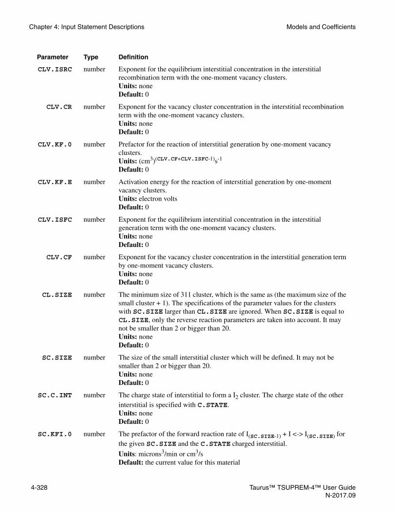
Chapter 4: Input Statement Descriptions Models and Coefficients

CLV.ISRC number Exponent for the equilibrium interstitial concentration in the interstitial recombination term with the one-moment vacancy clusters.Units: noneDefault: 0

CLV.CR number Exponent for the vacancy cluster concentration in the interstitial recombination term with the one-moment vacancy clusters.Units: noneDefault: 0

CLV.KF.0 number Prefactor for the reaction of interstitial generation by one-moment vacancy clusters.Units: (cm3)(CLV.CF+CLV.ISFC-1)s-1

Default: 0

CLV.KF.E number Activation energy for the reaction of interstitial generation by one-moment vacancy clusters.Units: electron voltsDefault: 0

CLV.ISFC number Exponent for the equilibrium interstitial concentration in the interstitial generation term with the one-moment vacancy clusters.Units: noneDefault: 0

CLV.CF number Exponent for the vacancy cluster concentration in the interstitial generation term by one-moment vacancy clusters.Units: noneDefault: 0

CL.SIZE number The minimum size of 311 cluster, which is the same as (the maximum size of the small cluster + 1). The specifications of the parameter values for the clusters with SC.SIZE larger than CL.SIZE are ignored. When SC.SIZE is equal to CL.SIZE, only the reverse reaction parameters are taken into account. It may not be smaller than 2 or bigger than 20.Units: none Default: 0

SC.SIZE number The size of the small interstitial cluster which will be defined. It may not be smaller than 2 or bigger than 20.Units: none Default: 0

SC.C.INT number The charge state of interstitial to form a I2 cluster. The charge state of the other interstitial is specified with C.STATE.Units: none Default: 0

SC.KFI.0 number The prefactor of the forward reaction rate of I(SC.SIZE-1) + I <-> I(SC.SIZE) for the given SC.SIZE and the C.STATE charged interstitial.

Units: microns3/min or cm3/s Default: the current value for this material

Parameter Type Definition

4-328 Taurus™ TSUPREM-4™ User GuideN-2017.09

Models and Coefficients Chapter 4: Input Statement Descriptions

SC.KFI.E number The activation energy of the forward reaction rate of I(SC.SIZE-1) + I <-> I(SC.SIZE) for the given SC.SIZE and the C.STATE charged interstitial.Units: electron volts Default: the current value for this material

SC.KRI.0 number The prefactor of the reverse reaction rate of I(SC.SIZE-1) + I <-> I(SC.SIZE) for the given SC.SIZE and the C.STATE charged interstitial.

Units: min-1 or s-1 Default: the current value for this material

SC.KRI.E number The activation energy of the reverse reaction rate of I(SC.SIZE-1) + I <-> I(SC.SIZE) for the given SC.SIZE and the C.STATE charged interstitial.Units: electron volts Default: the current value for this material

SC.KFV.0 number The prefactor of the forward reaction rate of I(SC.SIZE-1) <-> I(SC.SIZE) + V for the given SC.SIZE and the C.VACANC charged vacancy.

Units: min-1 or s-1 Default: the current value for this material

SC.KFV.E number The activation energy of the forward reaction rate of I(SC.SIZE-1) <-> I(SC.SIZE) + V for the given SC.SIZE and the C.VACANC charged vacancy. Units: electron volts Default: the current value for this material

SC.KRV.0 number The prefactor of the reverse reaction rate of I(SC.SIZE-1) <-> I(SC.SIZE) + V for the given SC.SIZE and the C.VACANC charged vacancy.

Units: microns3/min or cm3/sDefault: the current value for this material

SC.KRV.E number The activation of the reverse reaction rate of I(SC.SIZE-1) <-> I(SC.SIZE) + V for the given SC.SIZE and the C.VACANC charged vacancy.Units: electron volts Default: the current value for this material

CL.INI.F number The fraction of interstitials that are clustered upon implantation. Redistributes interstitials that are remaining after the dopant-defect clusters are formed according to C1.INI.F. Applies only outside of the amorphized regions. Inside the amorphized regions, all interstitial clusters are destroyed. The value must be set in the range from 0.0 to 1.0.Units: noneDefault: 0Synonym: INIT.311

CL.EQUIL logical Specifies that the initial interstitial clusters will be initialized to the equilibrium concentration. Turning on CL.EQUIL precedes the specification of CL.INI.F.Default: the current value; initially false

Parameter Type Definition

Taurus™ TSUPREM-4™ User Guide 4-329N-2017.09

Chapter 4: Input Statement Descriptions Models and Coefficients

MIN.INIT number Reset the minimum concentration to improve convergence in rebalancing the point-defect concentrations for initialization.

Units: cm-3

Default: 1e5

ECLUST.N number The number of interstitials in each small cluster.Units: noneDefault: the current value for this material

KLOOP.0 number The prefactor for KL in the dislocation loop model.Units: noneDefault: the current value for this material

Kloop.E number The activation energy for KL in the dislocation loop model.Units: electron voltsDefault: the current value for this material

RLMIN number The minimum radius for a dislocation loop; loops smaller than this size are removed from the simulation.Units: cmDefault: the current value for this material; initially 100e-8 cm

/MATERIA character The name of the second material for specifying interface injection and recombination parameters.Default: none

/SILICON logical The interface injection and recombination parameters apply to the interface between the specified material and silicon.Default: false

/OXIDE logical The interface injection and recombination parameters apply to the interface between the specified material and oxide. Default: false

/OXYNITR logical The interface injection and recombination parameters apply to the interface between the specified material and oxynitride. Default: false

/NITRIDE logical The interface injection and recombination parameters apply to the interface between the specified material and nitride. Default: false

/POLYSIL logical The interface injection and recombination parameters apply to the interface between the specified material and polysilicon. Default: false

/AMBIENT logical The interface injection and recombination parameters apply to the interface between the specified material and the ambient gas. Default: false Synonym: /GAS

Parameter Type Definition

4-330 Taurus™ TSUPREM-4™ User GuideN-2017.09

Models and Coefficients Chapter 4: Input Statement Descriptions

V.MAXOX logical Use the injection/recombination model, in which the interface velocity is normalized by the maximum interface velocity in the structure (the model used in older versions of TSUPREM-4).Default: the current value for these materials

V.INITOX logical Use the injection/recombination model, in which the interface velocity is normalized by the initial growth velocity for a bare silicon surface.Default: the current value for these materials

V.NORM logical Use the injection/recombination model, in which the interface velocity is normalized by the value specified by VNORM.0 and VNORM.E parameters.Default: the current value for these materials

KSURF.0 number The pre-exponential constant for the surface recombination velocity at the interface between the specified materials under inert conditions.Units: microns/min or cm/s Default: the current value for these materials Synonyms: KSMIN.0, KI.MIN

KSURF.E number The activation energy for the surface recombination velocity at the interface between the specified materials under inert conditions.Units: electron volts Default: the current value for these materials Synonym: KSMIN.E

KSURF.F character The user-defined expression of the recombination rate at material interfaces. The expression can be registered and applied under the MODEL parameter which is turned on/off in the METHOD statement.Units: noneDefault: “1.0”

KSVEL.0 number The pre-exponential constant for the growth-rate-dependent component of the surface recombination velocity at the interface between the specified materials. Used only with the V.MAXOX and V.NORM models.Units: microns/min or cm/s Default: the current value for these materials Synonyms: KSMAX.0, KI.MAX

KSVEL.E number The activation energy for the growth-rate-dependent component of the surface recombination velocity at the interface between the specified materials. Used only with the V.MAXOX and V.NORM models.Units: electron volts Default: the current value for these materials Synonym: KSMAX.E

KSRAT.0 number The pre-exponential constant for the ratio of the growth-rate-dependent component of the surface recombination velocity to the inert component at the interface between the specified materials. Used only with the V.INITOX model.Units: none Default: the current value for these materials

Parameter Type Definition

Taurus™ TSUPREM-4™ User Guide 4-331N-2017.09

Chapter 4: Input Statement Descriptions Models and Coefficients

KSRAT.E number The activation energy for the ratio of the growth-rate-dependent component of the surface recombination velocity to the inert component at the interface between the specified materials. Used only with the V.INITOX model.Units: electron volts Default: the current value for these materials

VNORM.0 number The pre-exponential constant for the normalization velocity in the V.NORM model.Units: microns/min or cm/s Default: the current value for these materials

VNORM.E number The activation energy for the normalization velocity in the V.NORM model.Units: electron volts Default: the current value for these materials

GROWTH logical Specifies that interstitial injection should be calculated using the computed velocities of the interface rather than the analytic model.Default: the current value for these materials

THETA.F character The user-defined expression of the injection rate at the interface of consumed silicon. The expression can be registered and applied under the MODEL parameter which is turned on/off in the METHOD statement.Units: noneDefault: “1.0”

THETA.0 number The pre-exponential constant for the fraction of consumed silicon atoms that are injected into the bulk as interstitials during oxidation.

Units: none, for V.INITOX and V.NORM models; (microns/min)(1-KPOW) or

(cm/s)(1-KPOW) for V.MAXOX modelDefault: the current value for these materials Synonym: THETA

THETA.E number The activation energy for the fraction of consumed silicon atoms that are injected into the bulk as interstitials during oxidation.Units: electron volts Default: the current value for these materials

A.0 number The pre-exponential constant for the injection rate of interstitials at the interface between the specified materials.

Units: #/micron2/min(1+GPOW) or #/cm2/s(1+GPOW) for V.INITOX and V.NORM

models; #/micron2/min(1-KPOW) or #/cm2/s(1-KPOW) for V.MAXOX model Default: the current value for these materials Synonym: A

A.E number The activation energy for the injection rate of interstitials at the interface between the specified materials.Units: electron volts Default: the current value for these materials

Parameter Type Definition

4-332 Taurus™ TSUPREM-4™ User GuideN-2017.09

Models and Coefficients Chapter 4: Input Statement Descriptions

T0.0 number The pre-exponential constant for the time constant for injection at the interface between the specified materials.Units: minutes or seconds Default: the current value for these materials Synonyms: T0

T0.E number The activation energy for the time constant for injection at the interface between the specified materials.Units: electron volts Default: the current value for these materials

KPOW.0 number The pre-exponential constant in the expression for the exponent in the surface recombination models. (Also used for injection with the V.MAXOX model.)Units: none Default: the current value for these materials Synonyms: TPOW.0, POWER

KPOW.E number The activation energy in the expression for the exponent in the surface recombination models. (Also used for injection with the V.MAXOX model.)Units: electron volts Default: the current value for these materials Synonym: TPOW.E

GPOW.0 number The pre-exponential constant in the expression for the exponent in the V.INITOX and V.NORM models for interstitial injection. Units: none Default: the current value for these materials

GPOW.E number The activation energy in the expression for the exponent in the V.INITOX and V.NORM models for interstitial injection.Units: electron volts Default: the current value for these materials

N.MAX.0 number The pre-exponential constant in the expression for the exponent in the maximum trapping site of nitrogen for interstitial recombination.

Units: /cm2

Default: the current value for these materials

N.MAX.E number The activation energy in the expression for the exponent in the maximum trapping site of nitrogen for interstitial recombination.Units: electron volts Default: the current value for these materials

CM.SEC logical If true, parameters involving time are specified in centimeters and seconds; if false, parameters involving time are in microns and minutes. Default: false

Parameter Type Definition

Taurus™ TSUPREM-4™ User Guide 4-333N-2017.09

Chapter 4: Input Statement Descriptions Models and Coefficients

Description This statement specifies values for coefficients of interstitial diffusion, recombination, injection, equilibrium concentration, and interstitial trap parameters. These parameters are normally specified in the s4init file (which is read when the program starts up), but can be changed by you at any time. Values that have not been set in s4init or by the user, default to 0.0.

Parameters whose units include time are specified in microns and minutes, unless CM.SEC is true, in which case units of centimeters and seconds are assumed.

The interpretation of the various parameters on the INTERSTITIAL statement is described in Chapter 3, Dose Loss Model, p. 3-67.

Bulk andInterface

Parameters

If bulk parameters (for example, D.0 or CEQUIL.E) are specified but no material is given, the parameters are assumed to apply to silicon. If interface parameters (for example, KSVEL.0 or A.E) are specified and only a “first” material (for example, OXIDE) is given, the parameters are assumed to apply to the interface between silicon and the specified material. This usage is not recommended, and is intended only for compatibility with older releases of TSUPREM-4.

Examples 1. The following statement specifies the silicon diffusivity and equilibrium values for interstitials:

INTERSTITIAL SILICON D.0=3000 CEQUIL.0=1.0e13

2. The following statement causes the Si/SiO2 interface injection is to be computed using the oxide growth velocity, with 1% of consumed silicon injected as interstitials:

INTERSTITIAL SILICON /OXIDE GROWTH THETA.0=0.01

3. The following statement specifies that the surface recombination velocity in the silicon at the interface with nitride is 3.5ex10-3 cm/s

INTERSTITIAL SILICON /NITRIDE CM.SEC +KSURF.0=3.5e-3 KSURF.E=0.0

4. The following statement specifies that the ratio of doubly-positive interstitials to neutral interstitials is 0.1 under intrinsic conditions:

INTERSTITIAL SILICON C.STATE=2 FRAC.0=0.1 FRAC.E=0.0

The C.STATE, FRAC.0, and FRAC.E parameters can be used to specify the fraction of interstitials in any charge state from -6 to +6.

MODEL character The name of the model to which the parameters for user-defined expressions, that is, D.FACTOR, D.F11, D.F22, KSURF.F and THETA.F, are registered. The ENABLE parameter, with the MODEL parameter given by this name in the METHOD statement, specifies the user-defined models related with the model are to be applied.Default: none

Parameter Type Definition

4-334 Taurus™ TSUPREM-4™ User GuideN-2017.09

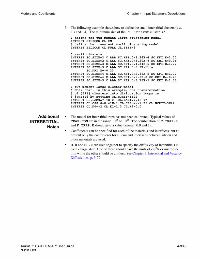
Models and Coefficients Chapter 4: Input Statement Descriptions

5. The following example shows how to define the small interstitial clusters (I2, I3 and I4). The minimum size of the cl_interst cluster is 5.

$ define the two-moment large clustering modelINTERST SILICON CL.2M $ define the transient small clustering modelINTERST SILICON CL.FULL CL.SIZE=5

$ small clustersINTERST SC.SIZE=2 C.ALL SC.KFI.0=1.26E-4 SC.KFI.E=1.77INTERST SC.SIZE=2 C.ALL SC.KRI.0=5.20E-8 SC.KRI.E=0.06INTERST SC.SIZE=3 C.ALL SC.KFI.0=1.34E-5 SC.KFI.E=1.77INTERST SC.SIZE=3 C.ALL SC.KRI.0=6.9E-11 +

SC.KRI.E=-0.23INTERST SC.SIZE=4 C.ALL SC.KFI.0=2.86E-5 SC.KFI.E=1.77INTERST SC.SIZE=4 C.ALL SC.KRI.0=9.0E-8 SC.KRI.E=-0.28INTERST SC.SIZE=5 C.ALL SC.KFI.0=3.78E-5 SC.KFI.E=1.77

$ two-moment large cluster model$ Note that, in this example, the transformation$ of {311} clusters into dislocation loops is $ ignored by setting CL.NCRIT=5E22INTERST CL.LAM0=7.4E-07 CL.LAM1=7.4E-07INTERST CL.CSS.0=8.41E-3 CL.CSS.e=-1.25 CL.NCRIT=5E22INTERST CL.K0=-2 CL.K1=1.0 CL.K2=0.0

AdditionalINTERSTITIAL

Notes

• The model for interstitial traps has not been calibrated. Typical values of TRAP.CON are in the range 1015 to 1018. The combination of F.TRAP.0 and F.TRAP.E should give a value between 0.0 and 1.0.

• Coefficients can be specified for each of the materials and interfaces, but at present only the coefficients for silicon and interfaces between silicon and other materials are used.

• D.0 and DC.0 are used together to specify the diffusivity of interstitials in each charge state. One of these should have the units of cm2/s or microns2/min while the other should be unitless. See Chapter 3, Interstitial and Vacancy Diffusivities, p. 3-72.

Taurus™ TSUPREM-4™ User Guide 4-335N-2017.09

Chapter 4: Input Statement Descriptions Models and Coefficients

VACANCY

The VACANCY statement sets the coefficients for vacancy kinetics.

VACANCY

{MATERIAL=<c> | SILICON | OXIDE | OXYNITRI | NITRIDE | POLYSILI | AMBIENT} [D.0=<n>] [D.E=<n>] [D.FACTOR=<c>] [D.F11=<c>] [D.F22=<c>]

[VD=<n>] [CEQUIL.0=<n>] [CEQUIL.E=<n>] [CEQUIL.F=<c>] [VCEQUIL=<n>][{CL.NONE|CL.1M}] [CL.FULL][VMOLE=<n>] [MODEL=<c>]

[NEU.0=<n>] [NEU.E=<n>] [NEG.0=<n>] [NEG.E=<n>] [DNEG.0=<n>] [DNEG.E=<n>] [POS.0=<n>] [POS.E=<n>][DPOS.0=<n>] [DPOS.E=<n>]

[ ( C.STATE=<n> [C.VACANC=<n>] )| C.ALL ][DC.0=<n>] [DC.E=<n>] [FRAC.0=<n>] [FRAC.E=<n>][KIC.0=<n>] [KIC.E=<n>] [ECLUST.0=<n>] [ECLUST.E=<n>] ][ECLUST.N=<n> ][CL.KF.0=<n>] [CL.KF.E=<n>] [CL.VF=<n>] [CL.VSF=<n>]

[CL.KFC.0=<n>] [CL.KFC.E=<n>] [CL.VFC=<n>] [CL.VSFC=<n>] [CL.KFC=<n>] [CL.CF=<n>] [CL.KR.0=<n>] [CL.KR.E=<n>] [CL.CR=<n>]

[CLI.KR.0=<n>] [CLI.KR.E=<n>] [CLI.VRC=<n>] [CLI.VSRC=<n>] [CLI.CR=<n>] [CLI.KF.0=<n>] [CLI.KF.E=<n>] [CLI.VSFC=<n>] [CLI.CF=<n>][CL.SIZE=<n>][ SC.SIZE=<n> [SC.C.VAC=<n>]

[SC.KFV.0=<n>] [SC.KFV.E=<n>] [SC.KRV.0=<n>] [SC.KRV.E=<n>][SC.KFI.0=<n>] [SC.KFI.E=<n>] [SC.KRI.0=<n>] [SC.KRI.E=<n>]

][CL.INI.F=<n>] [CL.EQUIL][MIN.INIT=<n>]

[{/MATERIA=<c> | /SILICON | /OXIDE | /OXYNITR | /NITRIDE | /POLYSIL | /AMBIENT}] [{V.MAXOX | V.INITOX | V.NORM}]

[KSURF.F=<c>] [KSURF.0=<n>] [KSURF.E=<n>] [KSVEL.0=<n>] [KSVEL.E=<n>] [KSRAT.0=<n>] [KSRAT.E=<n>] [VNORM.0=<n>] [VNORM.E=<n>] [GROWTH] [THETA.F=<c>] [THETA.0=<n>] [THETA.E=<n>] [A.0=<n>] [A.E=<n>] [T0.0=<n>] [T0.E=<n>] [KPOW.0=<n>] [KPOW.E=<n>] [GPOW.0=<n>] [GPOW.E=<n>]

[CM.SEC] [MODEL=<c>]

Parameter Type Definition

MATERIAL character The name of the material to which the other parameters apply.Default: none

4-336 Taurus™ TSUPREM-4™ User GuideN-2017.09

Models and Coefficients Chapter 4: Input Statement Descriptions

SILICON logical The other parameters apply to silicon. Default: true if no other material specified

OXIDE logical The other parameters apply to oxide. Default: false

OXYNITRI logical The other parameters apply to oxynitride. Default: false

NITRIDE logical The other parameters apply to nitride. Default: false

POLYSILI logical The other parameters apply to polysilicon. Default: false

AMBIENT logical The other parameters apply to the ambient gas. Default: false Synonym: GAS

D.0 number The pre-exponential constant for the diffusivity of vacancies in the specified material. Only used with SILICON. Units: microns2/min or cm2/s or noneDefault: the current value for this material Synonym: DI

D.E number The activation energy for the diffusivity of vacancies in the specified material. Only used with SILICON. Units: electron volts Default: the current value for this material

D.FACTOR character The user-defined expression of the isotropic multiplication factor of diffusivity. Only used with SILICON. The expression can be registered and applied under the MODEL parameter which is turned on/off in the METHOD statement.Units: noneDefault: the current value for this material

D.F11 character The user-defined expression of the anisotropic x-directional tensor multiplication factor of diffusivity. Only used with SILICON. The expression can be registered and applied under the MODEL parameter which is turned on/off in the METHOD statement.Units: noneDefault: the current value for this material

D.F22 character The user-defined expression of the anisotropic y-directional tensor multiplication factor of diffusivity. Only used with SILICON. The expression can be registered and applied under the MODEL parameter which is turned on/off in the METHOD statement.Units: noneDefault: the current value for this material

VD number The activation volume for the pressure-dependent diffusivityUnits: Å3

Default: the current value for this material

Parameter Type Definition

Taurus™ TSUPREM-4™ User Guide 4-337N-2017.09

Chapter 4: Input Statement Descriptions Models and Coefficients

CEQUIL.0 number The pre-exponential constant for equilibrium concentration of vacancies in the specified material. Only used with SILICON. Units: vacancies/cm3 Default: the current value for this material Synonym: CV

CEQUIL.E number The activation energy for equilibrium concentration of vacancies in the specified material. Only used with SILICON. Units: electron volts Default: the current value for this material

CEQUIL.F character The user-defined expression of the multiplication factor of an intrinsic equilibrium vacancy concentration. Only used with SILICON. The expression can be registered and applied under the MODEL parameter which is turned on/off in the METHOD statement.Units: noneDefault: the current value for this material

VCEQUIL number The activation volume for the pressure-dependent vacancy concentration in intrinsic equilibrium.Units: Å3

Default: the current value for this material

CL.NONE logical Disables the vacancy clustering model for the specified material.Default: the current value; initially true for all materials.

CL.1M logical Enables the 1-moment vacancy clustering model for the specified material.Default: the current value; initially false for all materials.Synonym: CL.MODEL

CL.FULL logical Enables the full transient small vacancy clustering model for the specified material.Default: the current value; initially false

VMOLE number The concentration of silicon atoms, used in the GROWTH model. Only used with SILICON. Units: atoms/cm3 Default: the current value for this material

NEU.0 number The pre-exponential constant for the relative concentration of neutral vacancies.Units: none Default: the current value for this material

NEU.E number The activation energy for the relative concentration of neutral vacancies.Units: electron volts Default: the current value for this material

NEG.0 number The pre-exponential constant for the relative concentration of negatively charged vacancies.Units: none Default: the current value for this material

Parameter Type Definition

4-338 Taurus™ TSUPREM-4™ User GuideN-2017.09

Models and Coefficients Chapter 4: Input Statement Descriptions

NEG.E number The activation energy for the relative concentration of negatively charged vacancies.Units: electron volts Default: the current value for this material

DNEG.0 number The pre-exponential constant for the relative concentration of doubly-negative charged vacancies.Units: none Default: the current value for this material

DNEG.E number The activation energy for the relative concentration of doubly-negative charged vacancies.Units: electron volts Default: the current value for this material

POS.0 number The pre-exponential constant for the relative concentration of positively charged vacancies.Units: none Default: the current value for this material

POS.E number The activation energy for the relative concentration of positively charged vacancies.Units: electron volts Default: the current value for this material

DPOS.0 number The pre-exponential constant for the relative concentration of doubly-positive charged vacancies.Units: none Default: the current value for this material

DPOS.E number The activation energy for the relative concentration of doubly-positive charged vacancies.Units: electron volts Default: the current value for this material

C.INTERS number The interstitial charge state to which the KIC.0, KIC.E, and vacancy clustering parameters apply. The value must be in the range of –6 to +6.Units: noneDefault: none

C.STATE number The vacancy charge state to which the DC.0, DC.E, FRAC.0, FRAC.E, KIC.0, KIC.E, ECLUST.0, ECLUST.E, and vacancy clustering parameters apply. The value must be in the range of –6 to +6.Units: noneDefault: noneSynonym: C.VACANC

C.ALL number Specifies that the DC.0, DC.E, FRAC.0, FRAC.E, KIC.0, KIC.E, ECLUST.0, ECLUST.E, and vacancy clustering parameters should be used for all charge states.Default: false

Parameter Type Definition

Taurus™ TSUPREM-4™ User Guide 4-339N-2017.09

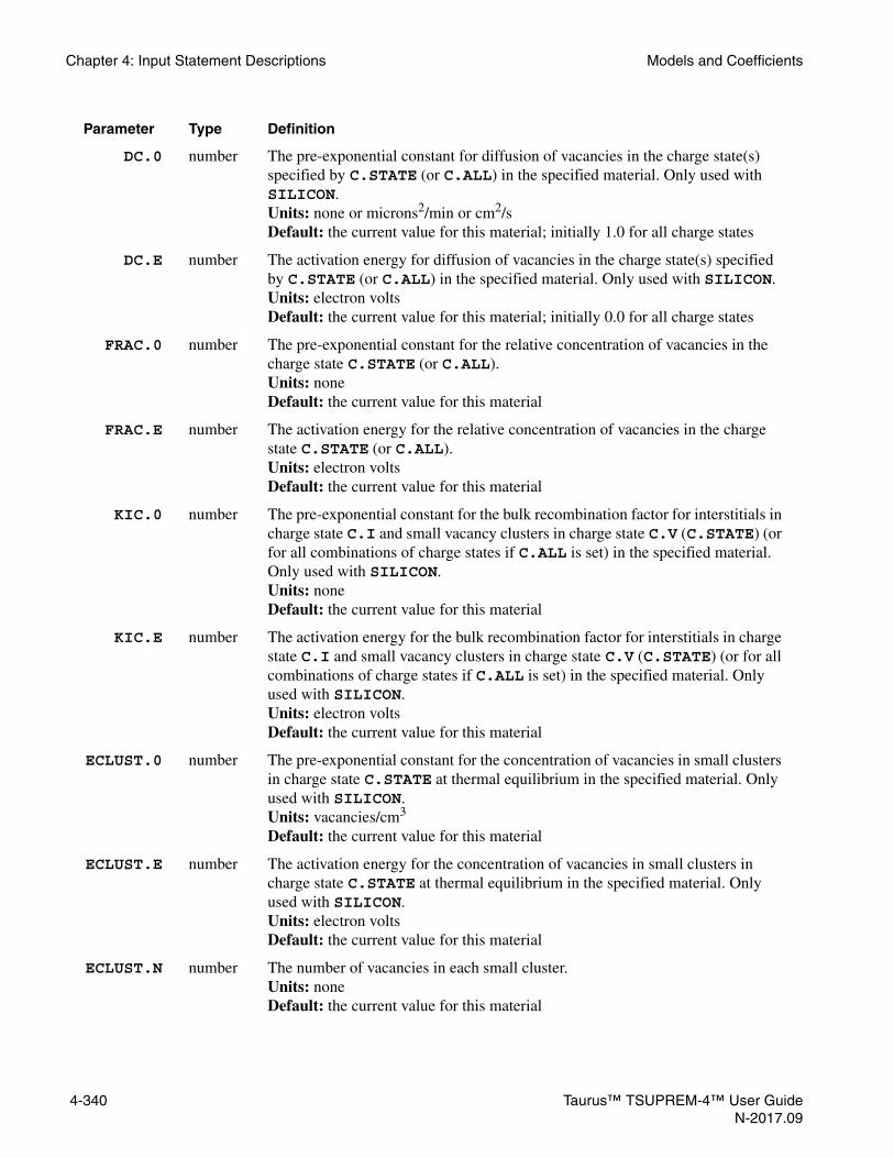
Chapter 4: Input Statement Descriptions Models and Coefficients

DC.0 number The pre-exponential constant for diffusion of vacancies in the charge state(s) specified by C.STATE (or C.ALL) in the specified material. Only used with SILICON. Units: none or microns2/min or cm2/s Default: the current value for this material; initially 1.0 for all charge states

DC.E number The activation energy for diffusion of vacancies in the charge state(s) specified by C.STATE (or C.ALL) in the specified material. Only used with SILICON. Units: electron volts Default: the current value for this material; initially 0.0 for all charge states

FRAC.0 number The pre-exponential constant for the relative concentration of vacancies in the charge state C.STATE (or C.ALL).Units: none Default: the current value for this material

FRAC.E number The activation energy for the relative concentration of vacancies in the charge state C.STATE (or C.ALL).Units: electron volts Default: the current value for this material

KIC.0 number The pre-exponential constant for the bulk recombination factor for interstitials in charge state C.I and small vacancy clusters in charge state C.V (C.STATE) (or for all combinations of charge states if C.ALL is set) in the specified material. Only used with SILICON. Units: noneDefault: the current value for this material

KIC.E number The activation energy for the bulk recombination factor for interstitials in charge state C.I and small vacancy clusters in charge state C.V (C.STATE) (or for all combinations of charge states if C.ALL is set) in the specified material. Only used with SILICON. Units: electron volts Default: the current value for this material

ECLUST.0 number The pre-exponential constant for the concentration of vacancies in small clusters in charge state C.STATE at thermal equilibrium in the specified material. Only used with SILICON. Units: vacancies/cm3

Default: the current value for this material

ECLUST.E number The activation energy for the concentration of vacancies in small clusters in charge state C.STATE at thermal equilibrium in the specified material. Only used with SILICON. Units: electron volts Default: the current value for this material

ECLUST.N number The number of vacancies in each small cluster.Units: noneDefault: the current value for this material

Parameter Type Definition

4-340 Taurus™ TSUPREM-4™ User GuideN-2017.09

Models and Coefficients Chapter 4: Input Statement Descriptions

CL.KF.0 number The prefactor for the Kfi (V+V→C) term in the vacancy clustering model. Units:

cm-(3*(1+CL.VSF-CL.VF))/sDefault: the current value for this material

CL.KF.E number The activation energy for the Kfi (V+V→C) term in the vacancy clustering model.Units: electron voltsDefault: the current value for this material

CL.VF number The power of the vacancy concentration in the Kfi (V+V→C) term in the vacancy clustering model. Units: noneDefault: the current value for this material

CL.VSF number The power of the equilibrium vacancy concentration in the Kfi (V+V→C) term in the vacancy clustering model.Units: noneDefault: the current value for this material

CL.KFC.0 number The prefactor for the Kfc (V+C→C) term in the vacancy clustering model.

Units: cm-(3*(1-CL.CF+CL.VSFC-CL.VFC))/sDefault: the current value for this material

CL.KFC.E number The activation energy for the Kfc (V+C→C) term in the vacancy clustering model.Units: electron voltsDefault: the current value for this material

CL.VFC number The power of the vacancy concentration in the Kfc (V+C→C) term in the vacancy clustering model.Units: noneDefault: the current value for this material

CL.VSFC number The power of the equilibrium vacancy concentration in the Kfc (V+C→C) term in the vacancy clustering model. Units: noneDefault: the current value for this material

CL.KFC number The fraction of the vacancy concentration to be included in the Kfc (V+C→C) term in the vacancy clustering model.Units: noneDefault: the current value for this material; initially 1.0

CL.CF number The power of the clustered vacancy concentration in the Kfc (V+C→C) term in the vacancy clustering model.Units: noneDefault: the current value for this material

Parameter Type Definition

Taurus™ TSUPREM-4™ User Guide 4-341N-2017.09

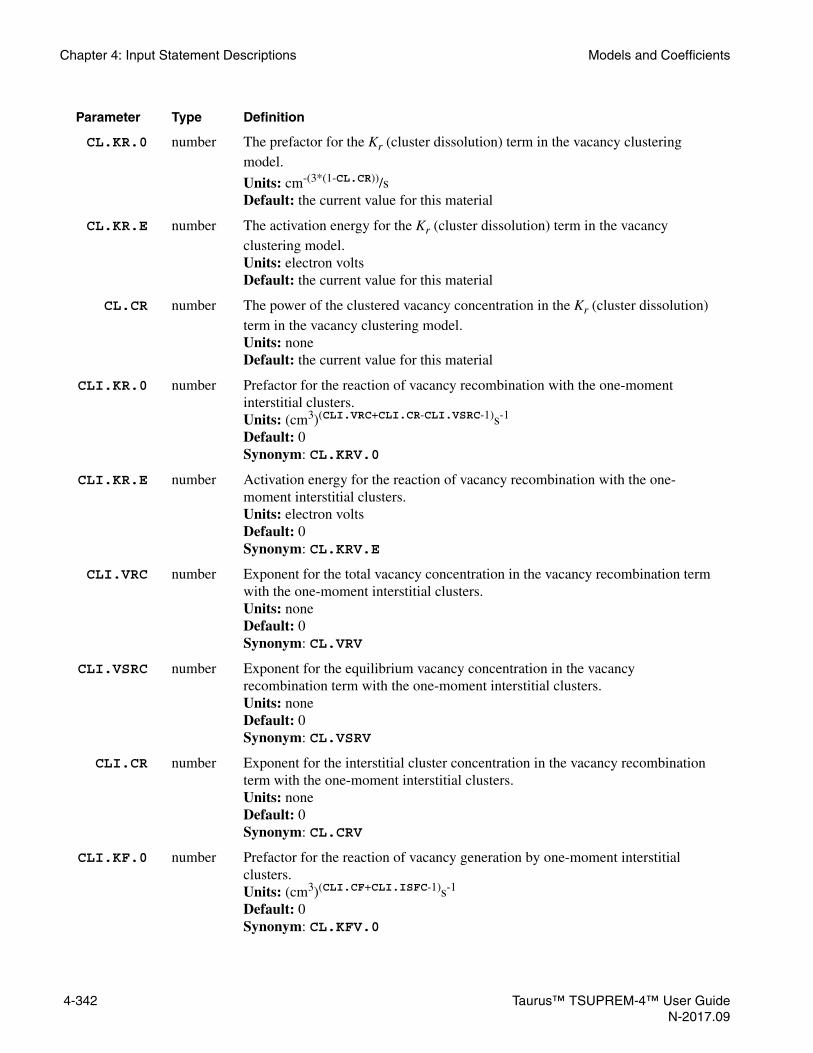
Chapter 4: Input Statement Descriptions Models and Coefficients

CL.KR.0 number The prefactor for the Kr (cluster dissolution) term in the vacancy clustering model.

Units: cm-(3*(1-CL.CR))/sDefault: the current value for this material

CL.KR.E number The activation energy for the Kr (cluster dissolution) term in the vacancy clustering model.Units: electron voltsDefault: the current value for this material

CL.CR number The power of the clustered vacancy concentration in the Kr (cluster dissolution) term in the vacancy clustering model.Units: noneDefault: the current value for this material

CLI.KR.0 number Prefactor for the reaction of vacancy recombination with the one-moment interstitial clusters.Units: (cm3)(CLI.VRC+CLI.CR-CLI.VSRC-1)s-1

Default: 0 Synonym: CL.KRV.0

CLI.KR.E number Activation energy for the reaction of vacancy recombination with the one-moment interstitial clusters.Units: electron voltsDefault: 0 Synonym: CL.KRV.E

CLI.VRC number Exponent for the total vacancy concentration in the vacancy recombination term with the one-moment interstitial clusters.Units: noneDefault: 0Synonym: CL.VRV

CLI.VSRC number Exponent for the equilibrium vacancy concentration in the vacancy recombination term with the one-moment interstitial clusters.Units: noneDefault: 0 Synonym: CL.VSRV

CLI.CR number Exponent for the interstitial cluster concentration in the vacancy recombination term with the one-moment interstitial clusters.Units: noneDefault: 0 Synonym: CL.CRV

CLI.KF.0 number Prefactor for the reaction of vacancy generation by one-moment interstitial clusters.Units: (cm3)(CLI.CF+CLI.ISFC-1)s-1

Default: 0 Synonym: CL.KFV.0

Parameter Type Definition

4-342 Taurus™ TSUPREM-4™ User GuideN-2017.09

Models and Coefficients Chapter 4: Input Statement Descriptions

CLI.KF.E number Activation energy for the reaction of vacancy generation by one-moment interstitial clusters.Units: electron voltsDefault: 0 Synonym: CL.KFV.E

CLI.VSFC number Exponent for the equilibrium vacancy concentration in the vacancy generation term with the one-moment interstitial clusters.Units: noneDefault: 0 Synonym: CL.VSFV

CLI.CF number Exponent for the interstitial cluster concentration in the vacancy generation term by one-moment interstitial clusters.Units: noneDefault: 0 Synonym: CL.CFV

CL.SIZE number The minimum size of large vacancy cluster, which is the same as (the maximum size of the small cluster + 1). The specifications of the parameter values for the clusters with SC.SIZE larger than CL.SIZE are ignored. When SC.SIZE is equal to CL.SIZE, only the reverse reaction parameters are taken into account. It may not be smaller than 2 or bigger than 20.Units: none Default: 0

SC.SIZE number The size of the small vacancy cluster which will be defined. It may not be smaller than 2 or bigger than 20.Units: none Default: 0

SC.C.VAC number The charge state of vacancy to form a V2 cluster. The charge state of the other vacancy is specified with C.STATE.Units: none Default: 0

SC.KFV.0 number The prefactor of the forward reaction rate of V(SC.SIZE-1) + V<-> V(SC.SIZE) for the given SC.SIZE and the C.STATE charged vacancy.

Units: microns3/min or cm3/s Default: the current value for this material

SC.KFV.E number The activation energy of the forward reaction rate of V(SC.SIZE-1) + V<-> V(SC.SIZE) for the given SC.SIZE and the C.STATE charged vacancy.Units: electron volts Default: the current value for this material

SC.KRV.0 number The prefactor of the reverse reaction rate of V(SC.SIZE-1) + V<-> V(SC.SIZE) for the given SC.SIZE and the C.STATE charged vacancy.

Units: min-1 or s-1 Default: the current value for this material

Parameter Type Definition

Taurus™ TSUPREM-4™ User Guide 4-343N-2017.09

Chapter 4: Input Statement Descriptions Models and Coefficients

SC.KRV.E number The activation energy of the reverse reaction rate of V(SC.SIZE-1) + V<-> V(SC.SIZE) for the given SC.SIZE and the C.STATE charged vacancy.Units: electron volts Default: the current value for this material

SC.KFI.0 number The prefactor of the forward reaction rate of V(SC.SIZE-1) <-> V(SC.SIZE) + I for the given SC.SIZE and the C.INTERS charged interstitial.

Units: min-1 or s-1 Default: the current value for this material

SC.KFI.E number The activation energy of the forward reaction rate of V(SC.SIZE-1) <-> V(SC.SIZE) + I for the given SC.SIZE and the C.INTERS charged interstitial. Units: electron volts Default: the current value for this material

SC.KRI.0 number The prefactor of the reverse reaction rate of V(SC.SIZE-1) <-> V(SC.SIZE) + I for the given SC.SIZE and the C.INTERS charged interstitial.

Units: microns3/min or cm3/sDefault: the current value for this material

SC.KRI.E number The activation of the reverse reaction rate of V(SC.SIZE-1) <-> V(SC.SIZE) + I for the given SC.SIZE and the C.VINTERS charged interstitial.Units: electron volts Default: the current value for this material

CL.INI.F number The fraction of interstitials that are clustered upon implantation. Redistributes interstitials that are remaining after the dopant-defect clusters are formed according to C1.INI.F. Applies only outside of the amorphized regions. Inside the amorphized regions, all vacancy clusters are destroyed. The value must be set in the range from 0.0 to 1.0.Units: noneDefault: 0

CL.EQUIL logical Specifies that the initial vacancy clusters will be initialized to the equilibrium concentration. Turning on CL.EQUIL precedes the specification of CL.INI.F.Default: the current value; initially false

MIN.INIT number Reset the minimum concentration to improve convergence in rebalancing the point-defect concentrations for initialization.

Units: cm-3

Default: le5

/MATERIA character The name of the second material for specifying interface injection and recombination parameters.Default: none

/SILICON logical The interface injection and recombination parameters apply to the interface between the specified material and silicon.Default: false

Parameter Type Definition

4-344 Taurus™ TSUPREM-4™ User GuideN-2017.09

Models and Coefficients Chapter 4: Input Statement Descriptions

/OXIDE logical The interface injection and recombination parameters apply to the interface between the specified material and oxide. Default: false

/OXYNITR logical The interface injection and recombination parameters apply to the interface between the specified material and oxynitride. Default: false

/NITRIDE logical The interface injection and recombination parameters apply to the interface between the specified material and nitride. Default: false

/POLYSIL logical The interface injection and recombination parameters apply to the interface between the specified material and polysilicon. Default: false

/AMBIENT logical The interface injection and recombination parameters apply to the interface between the specified material and the ambient gas. Default: false Synonym: /GAS

V.MAXOX logical Use the injection/recombination model, in which the interface velocity is normalized by the maximum interface velocity in the structure (the model used in older versions of TSUPREM-4).Default: the current value for these materials

V.INITOX logical Use the injection/recombination model, in which the interface velocity is normalized by the initial growth velocity for a bare silicon surface.Default: the current value for these materials

V.NORM logical Use the injection/recombination model, in which the interface velocity is normalized by the value specified by VNORM.0 and VNORM.E parameters.Default: the current value for these materials

KSURF.F character The user-defined expression of the recombination rate at material interfaces. The expression can be registered and applied under the MODEL parameter which is turned on/off in the METHOD statement.Units: noneDefault: “1.0”

KSURF.0 number The pre-exponential constant for the surface recombination velocity at the interface between the specified materials under inert conditions.Units: microns/min or cm/s Default: the current value for these materials Synonyms: KSMIN.0, KV.MIN

KSURF.E number The activation energy for the surface recombination velocity at the interface between the specified materials under inert conditions.Units: electron volts Default: the current value for these materials Synonym: KSMIN.E

Parameter Type Definition

Taurus™ TSUPREM-4™ User Guide 4-345N-2017.09

Chapter 4: Input Statement Descriptions Models and Coefficients

KSVEL.0 number The pre-exponential constant for the growth-rate-dependent component of the surface recombination velocity at the interface between the specified materials. Used only with the V.MAXOX and V.NORM models.Units: microns/min or cm/s Default: the current value for these materials Synonyms: KSMAX.0, KV.MAX

KSVEL.E number The activation energy for the growth-rate-dependent component of the surface recombination velocity at the interface between the specified materials. Used only with the V.MAXOX and V.NORM models.Units: electron volts Default: the current value for these materials Synonym: KSMAX.E

KSRAT.0 number The pre-exponential constant for the ratio of the growth-rate-dependent component of the surface recombination velocity to the inert component at the interface between the specified materials. Used only with the V.INITOX model.Units: none Default: the current value for these materials

KSRAT.E number The activation energy for the ratio of the growth-rate-dependent component of the surface recombination velocity to the inert component at the interface between the specified materials. Used only with the V.INITOX model.Units: electron volts Default: the current value for these materials

VNORM.0 number The pre-exponential constant for the normalization velocity in the V.NORM model.Units: microns/min or cm/s Default: the current value for these materials

VNORM.E number The activation energy for the normalization velocity in the V.NORM model.Units: electron volts Default: the current value for these materials

GROWTH logical Specifies that vacancy injection should be calculated using the computed velocities of the interface rather than the analytic model.Default: the current value for these materials

THETA.F character The user-defined expression of the injection rate at the interface of consumed silicon. The expression can be registered and applied under the MODEL parameter which is turned on/off in the METHOD statement.Units: noneDefault: “1.0”

THETA.0 number The pre-exponential constant for the number of vacancies injected into the bulk per consumed silicon atom during oxidation.Units: none, for V.INITOX and V.NORM models; (microns/min)(1-KPOW) or (cm/s)(1-KPOW) for V.MAXOX modelDefault: the current value for these materials Synonyms: THETA

Parameter Type Definition

4-346 Taurus™ TSUPREM-4™ User GuideN-2017.09

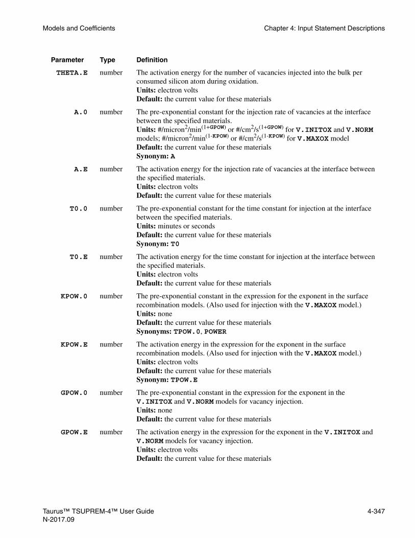
Models and Coefficients Chapter 4: Input Statement Descriptions

THETA.E number The activation energy for the number of vacancies injected into the bulk per consumed silicon atom during oxidation.Units: electron volts Default: the current value for these materials

A.0 number The pre-exponential constant for the injection rate of vacancies at the interface between the specified materials.Units: #/micron2/min(1+GPOW) or #/cm2/s(1+GPOW) for V.INITOX and V.NORM models; #/micron2/min(1-KPOW) or #/cm2/s(1-KPOW) for V.MAXOX model Default: the current value for these materialsSynonym: A

A.E number The activation energy for the injection rate of vacancies at the interface between the specified materials.Units: electron volts Default: the current value for these materials

T0.0 number The pre-exponential constant for the time constant for injection at the interface between the specified materials.Units: minutes or seconds Default: the current value for these materials Synonym: T0

T0.E number The activation energy for the time constant for injection at the interface between the specified materials.Units: electron volts Default: the current value for these materials

KPOW.0 number The pre-exponential constant in the expression for the exponent in the surface recombination models. (Also used for injection with the V.MAXOX model.)Units: none Default: the current value for these materials Synonyms: TPOW.0, POWER

KPOW.E number The activation energy in the expression for the exponent in the surface recombination models. (Also used for injection with the V.MAXOX model.)Units: electron volts Default: the current value for these materials Synonym: TPOW.E

GPOW.0 number The pre-exponential constant in the expression for the exponent in the V.INITOX and V.NORM models for vacancy injection.Units: none Default: the current value for these materials

GPOW.E number The activation energy in the expression for the exponent in the V.INITOX and V.NORM models for vacancy injection.Units: electron volts Default: the current value for these materials

Parameter Type Definition

Taurus™ TSUPREM-4™ User Guide 4-347N-2017.09

Chapter 4: Input Statement Descriptions Models and Coefficients

Description This statement specifies values for coefficients of vacancy diffusion, recombination, injection, and equilibrium concentration. These parameters are normally specified in the s4init file (which is read when the program starts up) but can be changed by you at any time. Values that have not been set in s4init or by the user, default to 0.0.

Parameters whose units include time are specified in units of microns and minutes, unless CM.SEC is true, in which case units of centimeters and seconds are assumed.

The interpretation of the various parameters on the VACANCY statement is described in Chapter 3, Dose Loss Model, p. 3-67.

Bulk andInterface

Parameters

If bulk parameters (for example, D.0 or CEQUIL.E) are specified but no material is given, the parameters are assumed to apply to silicon. If interface parameters (for example, KSVEL.0 or A.E) are specified and only a “first” material (for example, OXIDE) is given, the parameters are assumed to apply to the interface between silicon and the specified material. This usage is not recommended, and is intended only for compatibility with older releases of TSUPREM-4.

Examples 1. The following statement specifies the silicon diffusivity and equilibrium values for vacancies:

VACANCY SILICON D.0=3000 CEQUIL.0=1.0e13

2. The following statement causes the Si/SiO2 interface injection to be computed using the oxide growth velocity, with 1% of consumed silicon injected as vacancies

VACANCY SILICON /OXIDE GROWTH THETA.0=0.01

3. The following statement specifies that the surface recombination velocity in the silicon at the interface with nitride is 3.5x10-3 cm/s:

VACANCY SILICON /NITRIDE CM.SEC KSURF.0=3.5e-3 +KSURF.E=0.0

CM.SEC logical If true, parameters involving time are specified in centimeters and seconds; if false, parameters involving time are in microns and minutes. Default: false

MODEL character The name of the model to which the parameters for user-defined expressions, that is, D.FACTOR, D.F11, D.F22, KSURF.F and THETA.F, are registered. The ENABLE parameter, with the MODEL parameter given by this name in the METHOD statement, specifies the user-defined models related with the model are to be applied.Default: none

Parameter Type Definition

4-348 Taurus™ TSUPREM-4™ User GuideN-2017.09

Models and Coefficients Chapter 4: Input Statement Descriptions

4. The following statement specifies that the ratio of doubly-positive vacancies to neutral vacancies is 0.1 under intrinsic conditions:

VACANCY SILICON C.STATE=2 FRAC.0=0.1 FRAC.E=0.0

The C.STATE, FRAC.0, and FRAC.E parameters can be used to specify the fraction of interstitials in any charge state from -6 to +6.

AdditionalVACANCY Notes

• Coefficients can be specified for each of the materials, but some coefficients are only used for silicon and others apply to interfaces between silicon and other materials.

• D.0 and DC.0 are used together to specify the diffusivity of vacancies in each charge state. One of these should have the units of cm2/s or microns2/min, while the other should be unitless. See Chapter 3, Reaction of Pairs With Point Defects, p. 3-73.

Taurus™ TSUPREM-4™ User Guide 4-349N-2017.09

Chapter 4: Input Statement Descriptions Models and Coefficients

ANTIMONY

The ANTIMONY statement sets some of the properties of antimony.

ANTIMONY {MATERIAL=<c> | SILICON | OXIDE | OXYNITRI | NITRIDE | POLYSILI | AMBIENT} [DIX.0=<n>] [DIX.E=<n>] [DIM.0=<n>] [DIM.E=<n>] [DVX.0=<n>] [DVX.E=<n>] [DVM.0=<n>] [DVM.E=<n>] [DIPAIR.0=<n>] [DIPAIR.E=<n>] [DVPAIR.0=<n>] [DVPAIR.E=<n>] [R.I.S=<n>] [E.I.S=<n>] [R.V.S=<n>] [E.V.S=<n>] [R.IP.V=<n>] [E.IP.V=<n>] [R.VP.I=<n>] [E.VP.I=<n>]

[ { IP.V.LOW | IP.V.MED | IP.V.HIG } ][ { VP.I.LOW | VP.I.MED | VP.I.HIG } ]

[SS.CLEAR] [SS.TEMP=<n> SS.CONC=<n>] [ {/MATERIA=<c> | /SILICON | /OXIDE | /OXYNITR | /NITRIDE | /POLYSIL | /AMBIENT} [SEG.0=<n>] [SEG.E=<n>] [TRANS.0=<n>] [TRANS.E=<n>]

[KSIP.0=<n>] [KSIP.E=<n>] [KSVP.0=<n>] [KSVP.E=<n>] ] [ES.RAND=<n> [ES.F.RAN=<n>]] [ES.100=<n> [ES.F.100=<n>]] [ES.110=<n> [ES.F.110=<n>]] [CM.SEC]

Parameter Type Definition

MATERIAL character The name of the material to which the other parameters apply (material 1 for the segregation terms). Default: none

SILICON logical Specifies that other parameters in this statement apply to antimony in silicon, and that silicon is material 1 for the segregation terms. Default: true if no other first material is specified.

OXIDE logical Specifies that other parameters in this statement apply to antimony in oxide, and that oxide is material 1 for the segregation terms. Default: false

OXYNITRI logical Specifies that other parameters in this statement apply to antimony in oxynitride, and that oxynitride is material 1 for the segregation terms. Default: false

NITRIDE logical Specifies that other parameters in this statement apply to antimony in nitride, and that nitride is material 1 for the segregation terms. Default: false

POLYSILI logical Specifies that other parameters in this statement apply to antimony in polysilicon, and that polysilicon is material 1 for the segregation terms. Default: false

4-350 Taurus™ TSUPREM-4™ User GuideN-2017.09

Models and Coefficients Chapter 4: Input Statement Descriptions

AMBIENT logical Specifies that the ambient gas is material 1 for the segregation terms. Default: falseSynonym: GAS

DIX.0 number The pre-exponential constant for diffusion of antimony with neutral interstitials. Units: microns2/min or cm2/s Default: the current value for this material

DIX.E number The activation energy for diffusion of antimony with neutral interstitials. Units: electron volts Default: the current value for this material

DIM.0 number The pre-exponential constant for diffusion of antimony with singly-negative interstitials. Units: microns2/min or cm2/s Default: the current value for this material

DIM.E number The activation energy for diffusion of antimony with singly-negative interstitials. Units: electron volts Default: the current value for this material

DVX.0 number The pre-exponential constant for diffusion of antimony with neutral vacancies. Units: microns2/min or cm2/s Default: the current value for this material

DVX.E number The activation energy for diffusion of antimony with neutral vacancies. Units: electron volts Default: the current value for this material

DVM.0 number The pre-exponential constant for diffusion of antimony with singly-negative vacancies. Units: microns2/min or cm2/s Default: the current value for this material

DVM.E number The activation energy for diffusion of antimony with singly-negative vacancies. Units: electron volts Default: the current value for this material

DIPAIR.0 number The pre-exponential constant for the diffusivity of antimony-interstitial pairs. Units: microns2/min or cm2/s Default: the current value for this material

DIPAIR.E number The activation energy for the diffusivity of antimony-interstitial pairs.Units: electron volts Default: the current value for this material

DVPAIR.0 number The pre-exponential constant for the diffusivity of antimony-vacancy pairs. Units: microns2/min or cm2/s Default: the current value for this material

DVPAIR.E number The activation energy for the diffusivity of antimony-vacancy pairs.Units: electron volts Default: the current value for this material

Parameter Type Definition

Taurus™ TSUPREM-4™ User Guide 4-351N-2017.09

Chapter 4: Input Statement Descriptions Models and Coefficients

R.I.S number The capture radius for the reaction between interstitials and substitutionalantimony atoms.Units: ÅDefault: the current value for this material

E.I.S number The barrier energy for the reaction between interstitials and substitutionalantimony atoms.Units: electron voltsDefault: the current value for this material

R.V.S number The capture radius for the reaction between vacancies and substitutionalantimony atoms.Units: ÅDefault: the current value for this material

E.V.S number The barrier energy for the reaction between vacancies and substitutionalantimony atoms.Units: electron voltsDefault: the current value for this material

R.IP.V number The capture radius for the reaction between antimony-interstitial pairs and vacancies.Units: ÅDefault: the current value for this material

E.IP.V number The barrier energy for the reaction between antimony-interstitial pairs and vacancies.Units: electron voltsDefault: the current value for this material

R.VP.I number The capture radius for the reaction between antimony-vacancy pairs andinterstitials.Units: ÅDefault: the current value for this material

E.VP.I number The barrier energy for the reaction between antimony-vacancy pairs andinterstitials.Units: electron voltsDefault: the current value for this material

IP.V.LOW logical Assumes that only dopant-interstitial pairs and vacancies having opposite charges of equal magnitude react in bulk material.Default: true

IP.V.MED logical Assumes that uncharged dopant-interstitial pairs (or vacancies) can react with vacancies (or dopant-interstitial pairs) in any charged state, and that oppositely charged dopant-interstitial pairs and vacancies can react.Default: false

IP.V.HIG logical Assumes that dopant-vacancy pairs in any charged state can react with interstitials in any charged state.Default: false

Parameter Type Definition

4-352 Taurus™ TSUPREM-4™ User GuideN-2017.09

Models and Coefficients Chapter 4: Input Statement Descriptions

VP.I.LOW logical Assumes that only dopant-vacancy pairs and interstitials having opposite charges of equal magnitude react in bulk material.Default: true

VP.I.MED logical Assumes that uncharged dopant-vacancy pairs (or interstitials) can react with interstitials (or dopant-vacancy pairs) in any charged state, and that oppositely charged dopant-vacancy pairs and interstitials can react.Default: false

VP.I.HIG logical Assumes that dopant-vacancy pairs in any charged state can react with interstitials in any charged state.Default: false

SS.CLEAR logical Clears the solid solubility versus temperature table. Default: false

SS.TEMP number The temperature at which the solid solubility in material 1 is SS.CONC. Units: degrees Celsius Default: none

SS.CONC number The solid solubility in material 1 at temperature SS.TEMP. Units: atoms/cm3 Default: none

/MATERIA character The name of material 2 for the segregation parameters.Default: none

/SILICON logical Specifies that segregation parameters given on this statement apply to silicon as material 2. Default: false

/OXIDE logical Specifies that segregation parameters given on this statement apply to oxide as material 2. Default: True if no other second material is specified.

/OXYNITR logical Specifies that segregation parameters given on this statement apply to oxynitride as material 2. Default: true

/NITRIDE logical Specifies that segregation parameters given on this statement apply to nitride as material 2. Default: false

/POLYSIL logical Specifies that segregation parameters given on this statement apply topolysilicon as material 2. Default: false

/AMBIENT logical Specifies that segregation parameters given on this statement apply to theambient gas as material 2. Default: falseSynonym: /GAS

SEG.0 number The pre-exponential factor for segregation from material 1 to material 2. Units: none Default: the current value for these materials

Parameter Type Definition

Taurus™ TSUPREM-4™ User Guide 4-353N-2017.09

Chapter 4: Input Statement Descriptions Models and Coefficients

SEG.E number The activation energy for segregation from material 1 to material 2. Units: electron volts Default: the current value for these materials

TRANS.0 number The pre-exponential factor for transport from material 1 to material 2.Units: microns/min or cm/s Default: the current value for these materials Synonym: TRN.0

TRANS.E number The activation energy for transport from material 1 to material 2. Units: electron volts Default: the current value for these materialsSynonym: TRN.E

KSIP.0 number The pre-exponential constant for the surface recombination velocity of the dopant-interstitial pair at the interface between the specified materials.Units: microns/min or cm/sDefault: the current value for these materials

KSIP.E number The activation energy for the surface recombination velocity of the dopant-interstitial pair at the interface between the specified materialsUnits: electron voltsDefault: the current value for these materials

KSVP.0 number The pre-exponential constant for the surface recombination velocity of the dopant-vacancy pair at the interface between the specified materials.Units: microns/min or cm/sDefault: the current value for these materials

KSVP.E number The activation energy for the surface recombination velocity of the dopant-vacancy pair at the interface between the specified materialsUnits: electron voltsDefault: the current value for these materials

ES.RAND number The electronic stopping power coefficient of implanted antimony in the specified material for materials other than silicon and for a nonchanneled direction in silicon. This value is used for the MC ion implant calculation only.Units: angstrom2*eV(1-ES.F.RAN) Default: the current value for antimony and the specified material

ES.F.RAN number The exponent of the electronic stopping power of implanted antimony in the specified material for materials other than silicon and for a nonchanneled direction in silicon. This value is used for the MC ion implant calculation only.Units: none Default: the current value for antimony and the specified material

ES.100 number The electronic stopping power of antimony in silicon along the <100> channeling axes. This value is used for the MC ion implant calculation only.Units: angstrom2*eV(1-ES.F.100) Default: the current value for antimony and the specified material

Parameter Type Definition

4-354 Taurus™ TSUPREM-4™ User GuideN-2017.09

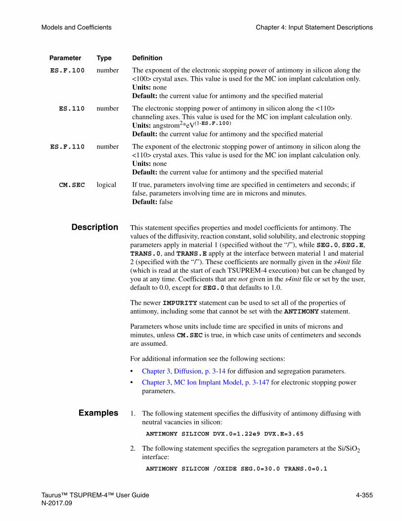
Models and Coefficients Chapter 4: Input Statement Descriptions

Description This statement specifies properties and model coefficients for antimony. The values of the diffusivity, reaction constant, solid solubility, and electronic stopping parameters apply in material 1 (specified without the “/”), while SEG.0, SEG.E, TRANS.0, and TRANS.E apply at the interface between material 1 and material 2 (specified with the “/”). These coefficients are normally given in the s4init file (which is read at the start of each TSUPREM-4 execution) but can be changed by you at any time. Coefficients that are not given in the s4init file or set by the user, default to 0.0, except for SEG.0 that defaults to 1.0.

The newer IMPURITY statement can be used to set all of the properties of antimony, including some that cannot be set with the ANTIMONY statement.

Parameters whose units include time are specified in units of microns and minutes, unless CM.SEC is true, in which case units of centimeters and seconds are assumed.

For additional information see the following sections:

• Chapter 3, Diffusion, p. 3-14 for diffusion and segregation parameters.

• Chapter 3, MC Ion Implant Model, p. 3-147 for electronic stopping power parameters.

Examples 1. The following statement specifies the diffusivity of antimony diffusing with neutral vacancies in silicon:

ANTIMONY SILICON DVX.0=1.22e9 DVX.E=3.65

2. The following statement specifies the segregation parameters at the Si/SiO2 interface:

ANTIMONY SILICON /OXIDE SEG.0=30.0 TRANS.0=0.1

ES.F.100 number The exponent of the electronic stopping power of antimony in silicon along the <100> crystal axes. This value is used for the MC ion implant calculation only.Units: none Default: the current value for antimony and the specified material

ES.110 number The electronic stopping power of antimony in silicon along the <110> channeling axes. This value is used for the MC ion implant calculation only.Units: angstrom2*eV(1-ES.F.100) Default: the current value for antimony and the specified material

ES.F.110 number The exponent of the electronic stopping power of antimony in silicon along the <110> crystal axes. This value is used for the MC ion implant calculation only. Units: none Default: the current value for antimony and the specified material

CM.SEC logical If true, parameters involving time are specified in centimeters and seconds; if false, parameters involving time are in microns and minutes. Default: false

Parameter Type Definition

Taurus™ TSUPREM-4™ User Guide 4-355N-2017.09

Chapter 4: Input Statement Descriptions Models and Coefficients

The concentration in silicon is 30.0 times the concentration in oxide, at equilibrium.

AdditionalANTIMONY

Notes

• The ANTIMONY statement has been made obsolete by the IMPURITY statement, but remains available for compatibility with existing input files. Note that some properties of antimony can only be set on the IMPURITY statement.

• The fractional interstitial parameter FI that was used in TSUPREM-4 before Version 6.0 is no longer supported. Instead, it is now necessary to specify the diffusivities with interstitials and vacancies separately.

4-356 Taurus™ TSUPREM-4™ User GuideN-2017.09

Models and Coefficients Chapter 4: Input Statement Descriptions

ARSENIC

The ARSENIC statement sets some of the properties of arsenic.

ARSENIC {MATERIAL=<c> | SILICON | OXIDE | OXYNITRI | NITRIDE | POLYSILI | AMBIENT} [DIX.0=<n>] [DIX.E=<n>] [DIM.0=<n>] [DIM.E=<n>] [DVX.0=<n>] [DVX.E=<n>] [DVM.0=<n>] [DVM.E=<n>] [DIPAIR.0=<n>] [DIPAIR.E=<n>] [DVPAIR.0=<n>] [DVPAIR.E=<n>] [R.I.S=<n>] [E.I.S=<n>] [R.V.S=<n>] [E.V.S=<n>] [R.IP.V=<n>] [E.IP.V=<n>] [R.VP.I=<n>] [E.VP.I=<n>]

[ { IP.V.LOW | IP.V.MED | IP.V.HIG } ][ { VP.I.LOW | VP.I.MED | VP.I.HIG } ]

[CTN.0=<n>] [CTN.E=<n>] [CTN.F=<n>] [ {/MATERIA=<c> | /SILICON | /OXIDE | /OXYNITR | /NITRIDE | /POLYSIL | /AMBIENT} [SEG.0=<n>] [SEG.E=<n>] [TRANS.0=<n>] [TRANS.E=<n>]

[KSIP.0=<n>] [KSIP.E=<n>] [KSVP.0=<n>] [KSVP.E=<n>] ] [ES.RAND=<n> [ES.F.RAN=<n>]] [ES.100=<n> [ES.F.100=<n>]] [ES.110=<n> [ES.F.110=<n>]] [CM.SEC]

Parameter Type Definition

MATERIAL character The name of the material to which the other parameters apply (material 1 for the segregation terms).Default: none

SILICON logical Specifies that other parameters in this statement apply to arsenic in silicon, and that silicon is material 1 for the segregation terms. Default: true if no other first material is specified.

OXIDE logical Specifies that other parameters in this statement apply to arsenic in oxide, and that oxide is material 1 for the segregation terms. Default: false

OXYNITRI logical Specifies that other parameters in this statement apply to arsenic in oxynitride, and that oxynitride is material 1 for the segregation terms. Default: false

NITRIDE logical Specifies that other parameters in this statement apply to arsenic in nitride, and that nitride is material 1 for the segregation terms. Default: false

POLYSILI logical Specifies that other parameters in this statement apply to arsenic in polysilicon, and that polysilicon is material 1 for the segregation terms. Default: false

Taurus™ TSUPREM-4™ User Guide 4-357N-2017.09

Chapter 4: Input Statement Descriptions Models and Coefficients

AMBIENT logical Specifies that the ambient gas is material 1 for the segregation terms. Default: false Synonym: GAS

DIX.0 number The pre-exponential constant for diffusion of arsenic with neutral interstitials. Units: microns2/min or cm2/sDefault: the current value for this material

DIX.E number The activation energy for diffusion of arsenic with neutral interstitials. Units: electron volts Default: the current value for this material

DIM.0 number The pre-exponential constant for diffusion of arsenic with singly-negative interstitials. Units: microns2/min or cm2/sDefault: the current value for this material

DIM.E number The activation energy for diffusion of arsenic with singly-negative interstitials. Units: electron volts Default: the current value for this material

DVX.0 number The pre-exponential constant for diffusion of arsenic with neutral vacancies. Units: microns2/min or cm2/sDefault: the current value for this material

DVX.E number The activation energy for diffusion of arsenic with neutral vacancies. Units: electron volts Default: the current value for this material

DVM.0 number The pre-exponential constant for diffusion of arsenic with singly-negative vacancies. Units: microns2/min or cm2/s Default: the current value for this material

DVM.E number The activation energy for diffusion of arsenic with singly-negative vacancies. Units: electron volts Default: the current value for this material

DIPAIR.0 number The pre-exponential constant for the diffusivity of arsenic-interstitial pairs. Units: microns2/min or cm2/s Default: the current value for this material

DIPAIR.E number The activation energy for the diffusivity of arsenic-interstitial pairs.Units: electron volts Default: the current value for this material

DVPAIR.0 number The pre-exponential constant for the diffusivity of arsenic-vacancy pairs. Units: microns2/min or cm2/s Default: the current value for this material

DVPAIR.E number The activation energy for the diffusivity of arsenic-vacancy pairs.Units: electron volts Default: the current value for this material

Parameter Type Definition

4-358 Taurus™ TSUPREM-4™ User GuideN-2017.09

Models and Coefficients Chapter 4: Input Statement Descriptions

R.I.S number The capture radius for the reaction between interstitials and substitutional arsenic atoms.Units: ÅDefault: the current value for this material

E.I.S number The barrier energy for the reaction between interstitials and substitutional arsenic atoms.Units: electron voltsDefault: the current value for this material

R.V.S number The capture radius for the reaction between vacancies and substitutional arsenic atoms.Units: ÅDefault: the current value for this material

E.V.S number The barrier energy for the reaction between vacancies and substitutional arsenic atoms.Units: electron voltsDefault: the current value for this material

R.IP.V number The capture radius for the reaction between arsenic-interstitial pairs and vacancies.Units: ÅDefault: the current value for this material

E.IP.V number The barrier energy for the reaction between arsenic-interstitial pairs and vacancies.Units: electron voltsDefault: the current value for this material

R.VP.I number The capture radius for the reaction between arsenic-vacancy pairs and interstitials.Units: ÅDefault: the current value for this material

E.VP.I number The barrier energy for the reaction between arsenic-vacancy pairs and interstitials.Units: electron voltsDefault: the current value for this material

IP.V.LOW logical Assumes that only dopant-interstitial pairs and vacancies having opposite charges of equal magnitude react in bulk material.Default: true

IP.V.MED logical Assumes that uncharged dopant-interstitial pairs (or vacancies) can react with vacancies (or dopant-interstitial pairs) in any charged state, and that oppositely charged dopant-interstitial pairs and vacancies can react.Default: false

IP.V.HIG logical Assumes that dopant-vacancy pairs in any charged state can react with interstitials in any charged state.Default: false

Parameter Type Definition

Taurus™ TSUPREM-4™ User Guide 4-359N-2017.09

Chapter 4: Input Statement Descriptions Models and Coefficients

VP.I.LOW logical Assumes that only dopant-vacancy pairs and interstitials having opposite charges of equal magnitude react in bulk material.Default: true

VP.I.MED logical Assumes that uncharged dopant-vacancy pairs (or interstitials) can react with interstitials (or dopant-vacancy pairs) in any charged state, and that oppositely charged dopant-vacancy pairs and interstitials can react.Default: false

VP.I.HIG logical Assumes that dopant-vacancy pairs in any charged state can react with interstitials in any charged state.Default: false

CTN.0 number The pre-exponential constant for clustering of arsenic. Units: (atoms/cm3)(1/CTN.F-1) Default: the current value for this material

CTN.E number The activation energy for clustering of arsenic. Units: electron volts Default: the current value for this material

CTN.F number The exponent of concentration for clustering of arsenic. Units: none Default: the current value for this material

/MATERIA character The name of material 2 for the segregation parameters.Default: none

/SILICON logical Specifies that segregation parameters given on this statement apply to silicon as material 2. Default: false

/OXIDE logical Specifies that segregation parameters given on this statement apply to oxide as material 2. Default: True if no other second material is specified.

/OXYNITR logical Specifies that segregation parameters given on this statement apply to oxynitride as material 2. Default: false

/NITRIDE logical Specifies that segregation parameters given on this statement apply to nitride as material 2. Default: false

/POLYSIL logical Specifies that segregation parameters given on this statement apply to polysilicon as material 2. Default: false

/AMBIENT logical Specifies that segregation parameters given on this statement apply to the ambient gas as material 2. Default: false Synonyms: /GAS

Parameter Type Definition

4-360 Taurus™ TSUPREM-4™ User GuideN-2017.09

Models and Coefficients Chapter 4: Input Statement Descriptions

SEG.0 number The pre-exponential factor for segregation from material 1 to material 2. Units: none Default: the current value for these materials

SEG.E number The activation energy for segregation from material 1 to material 2. Units: electron volts Default: the current value for these materials

TRANS.0 number The pre-exponential factor for transport from material 1 to material 2. Units: microns/min or cm/s Default: the current value for these materials Synonym: TRN.0

TRANS.E number The activation energy for transport from material 1 to material 2. Units: electron volts Default: the current value for these materials Synonym: TRN.E

KSIP.0 number The pre-exponential constant for the surface recombination velocity of the dopant-interstitial pair at the interface between the specified materials.Units: microns/min or cm/sDefault: the current value for these materials

KSIP.E number The activation energy for the surface recombination velocity of the dopant-interstitial pair at the interface between the specified materials.Units: electron voltsDefault: the current value for these materials

KSVP.0 number The pre-exponential constant for the surface recombination velocity of the dopant-vacancy pair at the interface between the specified materials.Units: microns/min or cm/sDefault: the current value for these materials

KSVP.E number The activation energy for the surface recombination velocity of the dopant-vacancy pair at the interface between the specified materials.Units: electron voltsDefault: the current value for these materials

ES.RAND number The electronic stopping power coefficient of implanted arsenic in the specified material for materials other than silicon and for a nonchanneled direction in silicon. This value is used for the MC ion implant calculation only.Units: angstrom2*eV(1-ES.F.RAN) Default: the current value for arsenic and the specified material

ES.F.RAN number The exponent of the electronic stopping power of implanted arsenic in the specified material for materials other than silicon and for a nonchanneled direction in silicon. This value is used for the MC ion implant calculation only.Units: none Default: the current value for arsenic and the specified material

Parameter Type Definition

Taurus™ TSUPREM-4™ User Guide 4-361N-2017.09

Chapter 4: Input Statement Descriptions Models and Coefficients

Description This statement specifies properties and model coefficients for arsenic. The values of the diffusivity, reaction constant, clustering, and electronic stopping parameters apply in material 1 (specified without the “/”), while SEG.0, SEG.E, TRANS.0 and TRANS.E apply at the interface between material 1 and material 2 (specified with the “/”). These coefficients are normally given in the s4init file (which is read at the start of each TSUPREM-4 execution), but can be changed by you at any time. Coefficients that are not given in the s4init file or set by the user, default to 0.0, except for SEG.0 that defaults to 1.0.

The newer IMPURITY statement can be used to set all of the properties of arsenic, including some that cannot be set with the ARSENIC statement.

Parameters whose units include time are specified in units of microns and minutes, unless CM.SEC is true, in which case units of centimeters and seconds are assumed.

For additional information, see:

• Chapter 3, Diffusion, p. 3-14 for diffusion and segregation parameters.

• Chapter 3, MC Ion Implant Model, p. 3-147 for electronic stopping power parameters.

ES.100 number The electronic stopping power of arsenic in silicon along the <100> channeling axes. This value is used for the MC ion implant calculation only.Units: angstrom2*eV(1-ES.F.100) Default: the current value for arsenic and the specified material

ES.F.100 number The exponent of the electronic stopping power of arsenic in silicon along the <100> crystal axes. This value is used for the MC ion implant calculation only.Units: none Default: the current value for arsenic and the specified material

ES.110 number The electronic stopping power of arsenic in silicon along the <110> channeling axes. This value is used for the MC ion implant calculation only. Units: angstrom2*eV(1-ES.F.100) Default: the current value for arsenic and the specified material

ES.F.110 number The exponent of the electronic stopping power of arsenic in silicon along the <110> crystal axes. This value is used for the MC ion implant calculation only.Units: none Default: the current value for arsenic and the specified material

CM.SEC logical If true, parameters involving time are specified in centimeters and seconds; if false, parameters involving time are in microns and minutes. Default: false

Parameter Type Definition

4-362 Taurus™ TSUPREM-4™ User GuideN-2017.09

Models and Coefficients Chapter 4: Input Statement Descriptions

Examples 1. The following statement specifies the diffusivity of arsenic diffusing with negative vacancies in silicon:

ARSENIC SILICON DVM.0=1.49e11 DVM.E=4.15

2. The following statement specifies the segregation parameters at the Si/SiO2 interface:

ARSENIC SILICON /OXIDE SEG.0=30.0 TRANS.0=0.1

The concentration in silicon is 30.0 times the concentration in oxide, at equilibrium.

AdditionalARSENIC Notes

1. The ARSENIC statement has been obsoleted by the IMPURITY statement, but remains available for compatibility with existing input files. Note that some properties of arsenic can only be set on the IMPURITY statement.

2. The fractional interstitial parameter FI that was used in TSUPREM-4 before Version 6.0 is no longer supported. Instead, it is now necessary to specify the diffusivities with interstitials and vacancies separately.

Taurus™ TSUPREM-4™ User Guide 4-363N-2017.09

Chapter 4: Input Statement Descriptions Models and Coefficients

BORON

The BORON statement sets some of the properties of boron.

BORON {MATERIAL=<c> | SILICON | OXIDE | OXYNITRI | NITRIDE | POLYSILI | AMBIENT} [DIX.0=<n>] [DIX.E=<n>] [DIP.0=<n>] [DIP.E=<n>] [DVX.0=<n>] [DVX.E=<n>] [DVP.0=<n>] [DVP.E=<n>] [DIPAIR.0=<n>] [DIPAIR.E=<n>] [DVPAIR.0=<n>] [DVPAIR.E=<n>] [R.I.S=<n>] [E.I.S=<n>] [R.V.S=<n>] [E.V.S=<n>] [R.IP.V=<n>] [E.IP.V=<n>] [R.VP.I=<n>] [E.VP.I=<n>]

[ { IP.V.LOW | IP.V.MED | IP.V.HIG } ][ { VP.I.LOW | VP.I.MED | VP.I.HIG } ]

[SS.CLEAR] [SS.TEMP=<n> SS.CONC=<n>] [ {/MATERIA=<c> | /SILICON | /OXIDE | /OXYNITR | /NITRIDE | /POLYSIL | /AMBIENT} [SEG.0=<n>] [SEG.E=<n>] [TRANS.0=<n>] [TRANS.E=<n>]

[KSIP.0=<n>] [KSIP.E=<n>] [KSVP.0=<n>] [KSVP.E=<n>] ] [ES.RAND=<n> [ES.F.RAN=<n>]] [ES.100=<n> [ES.F.100=<n>]] [ES.110=<n> [ES.F.110=<n>]] [CM.SEC]

Parameter Type Definition

MATERIAL character The name of the material to which the other parameters apply (material 1 for the segregation terms).Default: none

SILICON logical Specifies that other parameters in this statement apply to boron in silicon, and that silicon is material 1 for the segregation terms. Default: True if no other first material is specified.

OXIDE logical Specifies that other parameters in this statement apply to boron in oxide, and that oxide is material 1 for the segregation terms. Default: false

OXYNITRI logical Specifies that other parameters in this statement apply to boron in oxynitride, and that oxynitride is material 1 for the segregation terms. Default: false

NITRIDE logical Specifies that other parameters in this statement apply to boron in nitride, and that nitride is material 1 for the segregation terms. Default: false

POLYSILI logical Specifies that other parameters in this statement apply to boron in polysilicon, and that polysilicon is material 1 for the segregation terms. Default: false

4-364 Taurus™ TSUPREM-4™ User GuideN-2017.09

Models and Coefficients Chapter 4: Input Statement Descriptions

AMBIENT logical Specifies that the ambient gas is material 1 for the segregation terms. Default: false Synonym: GAS

DIX.0 number The pre-exponential constant for diffusion of boron with neutral interstitials. Units: microns2/min or cm2/s Default: the current value for this material

DIX.E number The activation energy for diffusion of boron with neutral interstitials. Units: electron volts Default: the current value for this material

DIP.0 number The pre-exponential constant for diffusion of boron with singly-positive interstitials. Units: microns2/min or cm2/s Default: the current value for this material

DIP.E number The activation energy for diffusion of boron with singly-positive interstitials. Units: electron volts Default: the current value for this material

DVX.0 number The pre-exponential constant for diffusion of boron with neutral vacancies. Units: microns2/min or cm2/s Default: the current value for this material

DVX.E number The activation energy for diffusion of boron with neutral vacancies. Units: electron volts Default: the current value for this material

DVP.0 number The pre-exponential constant for diffusion of boron with singly-positive vacancies. Units: microns2/min or cm2/s Default: the current value for this material

DVP.E number The activation energy for diffusion of boron with singly-positive vacancies. Units: electron volts Default: the current value for this material

DIPAIR.0 number The pre-exponential constant for the diffusivity of boron-interstitial pairs. Units: microns2/min or cm2/s Default: the current value for this material

DIPAIR.E number The activation energy for the diffusivity of boron-interstitial pairs.Units: electron volts Default: the current value for this material

DVPAIR.0 number The pre-exponential constant for the diffusivity of boron-vacancy pairs. Units: microns2/min or cm2/s Default: the current value for this material

DVPAIR.E number The activation energy for the diffusivity of boron-vacancy pairs.Units: electron volts Default: the current value for this material

Parameter Type Definition

Taurus™ TSUPREM-4™ User Guide 4-365N-2017.09

Chapter 4: Input Statement Descriptions Models and Coefficients

R.I.S number The capture radius for the reaction between interstitials and substitutional boron atoms.Units: ÅDefault: the current value for this material

E.I.S number The barrier energy for the reaction between interstitials and substitutional boron atoms.Units: electron voltsDefault: the current value for this material

R.V.S number The capture radius for the reaction between vacancies and substitutional boron atoms.Units: ÅDefault: the current value for this material

E.V.S number The barrier energy for the reaction between vacancies and substitutional boron atoms.Units: electron voltsDefault: the current value for this material

R.IP.V number The capture radius for the reaction between boron-interstitial pairs and vacancies.Units: ÅDefault: the current value for this material

E.IP.V number The barrier energy for the reaction between boron-interstitial pairs and vacancies.Units: electron voltsDefault: the current value for this material

R.VP.I number The capture radius for the reaction between boron-vacancy pairs and interstitials.Units: ÅDefault: the current value for this material

E.VP.I number The barrier energy for the reaction between boron-vacancy pairs and interstitials.Units: electron voltsDefault: the current value for this material

IP.V.LOW logical Assumes that only dopant-interstitial pairs and vacancies having opposite charges of equal magnitude react in bulk material.Default: true

IP.V.MED logical Assumes that uncharged dopant-interstitial pairs (or vacancies) can react with vacancies (or dopant-interstitial pairs) in any charged state, and that oppositely charged dopant-interstitial pairs and vacancies can react.Default: false

IP.V.HIG logical Assumes that dopant-vacancy pairs in any charged state can react with interstitials in any charged state.Default: false

Parameter Type Definition

4-366 Taurus™ TSUPREM-4™ User GuideN-2017.09

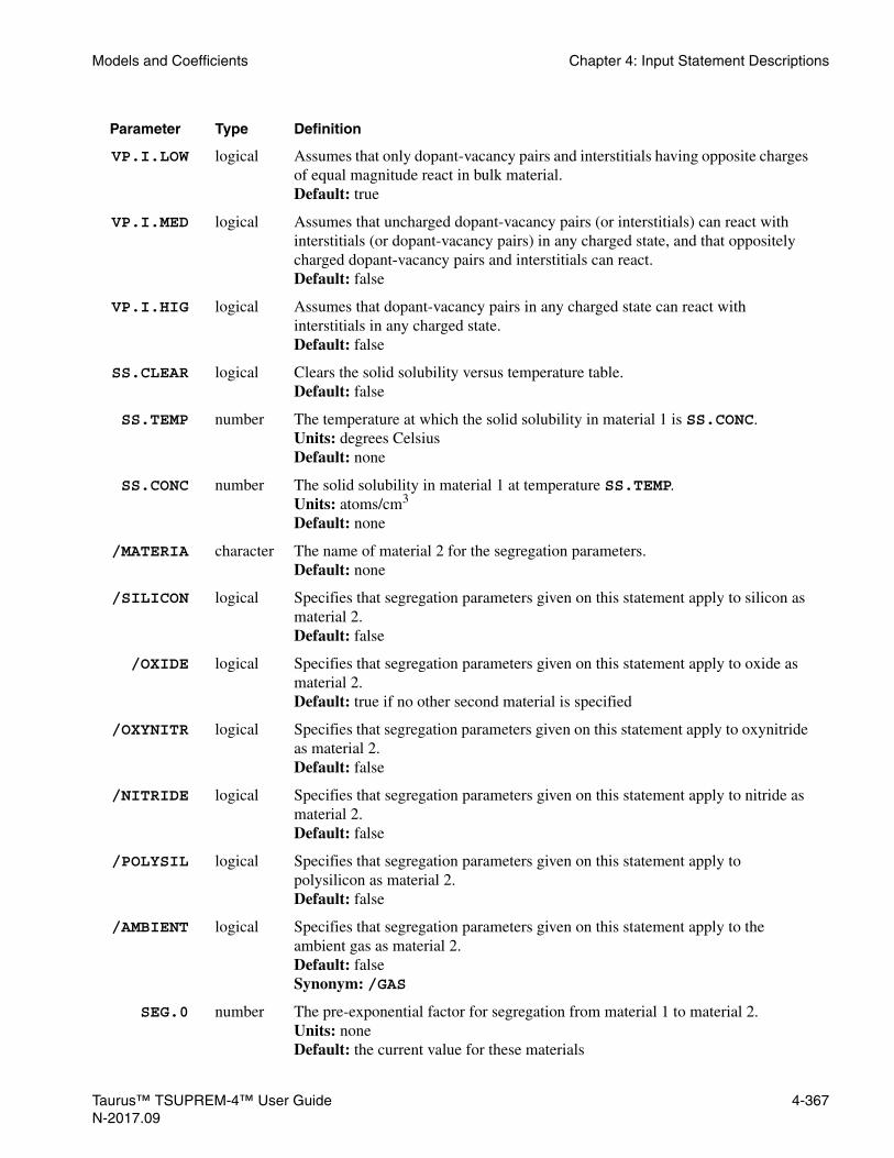
Models and Coefficients Chapter 4: Input Statement Descriptions

VP.I.LOW logical Assumes that only dopant-vacancy pairs and interstitials having opposite charges of equal magnitude react in bulk material.Default: true

VP.I.MED logical Assumes that uncharged dopant-vacancy pairs (or interstitials) can react with interstitials (or dopant-vacancy pairs) in any charged state, and that oppositely charged dopant-vacancy pairs and interstitials can react.Default: false

VP.I.HIG logical Assumes that dopant-vacancy pairs in any charged state can react with interstitials in any charged state.Default: false

SS.CLEAR logical Clears the solid solubility versus temperature table. Default: false

SS.TEMP number The temperature at which the solid solubility in material 1 is SS.CONC. Units: degrees Celsius Default: none

SS.CONC number The solid solubility in material 1 at temperature SS.TEMP. Units: atoms/cm3 Default: none

/MATERIA character The name of material 2 for the segregation parameters.Default: none

/SILICON logical Specifies that segregation parameters given on this statement apply to silicon as material 2. Default: false

/OXIDE logical Specifies that segregation parameters given on this statement apply to oxide as material 2. Default: true if no other second material is specified

/OXYNITR logical Specifies that segregation parameters given on this statement apply to oxynitride as material 2. Default: false

/NITRIDE logical Specifies that segregation parameters given on this statement apply to nitride as material 2. Default: false

/POLYSIL logical Specifies that segregation parameters given on this statement apply to polysilicon as material 2. Default: false

/AMBIENT logical Specifies that segregation parameters given on this statement apply to the ambient gas as material 2. Default: false Synonym: /GAS

SEG.0 number The pre-exponential factor for segregation from material 1 to material 2. Units: none Default: the current value for these materials

Parameter Type Definition

Taurus™ TSUPREM-4™ User Guide 4-367N-2017.09

Chapter 4: Input Statement Descriptions Models and Coefficients

SEG.E number The activation energy for segregation from material 1 to material 2. Units: electron volts Default: the current value for these materials

TRANS.0 number The pre-exponential factor for transport from material 1 to material 2.Units: microns/min or cm/s Default: the current value for these materials Synonym: TRN.0

TRANS.E number The activation energy for transport from material 1 to material 2. Units: electron volts Default: the current value for these materials Synonym: TRN.E

KSIP.0 number The pre-exponential constant for the surface recombination velocity of the dopant-interstitial pair at the interface between the specified materials.Units: microns/min or cm/sDefault: the current value for these materials

KSIP.E number The activation energy for the surface recombination velocity of the dopant-interstitial pair at the interface between the specified materialsUnits: electron voltsDefault: the current value for these materials

KSVP.0 number The pre-exponential constant for the surface recombination velocity of the dopant-vacancy pair at the interface between the specified materials.Units: microns/min or cm/sDefault: the current value for these materials

KSVP.E number The activation energy for the surface recombination velocity of the dopant-vacancy pair at the interface between the specified materialsUnits: electron voltsDefault: the current value for these materials

ES.RAND number The electronic stopping power coefficient of implanted boron in the specified material for materials other than silicon and for a nonchanneled direction in silicon. This value is used for the MC ion implant calculation only.Units: angstrom2*eV(1-ES.F.RAN) Default: the current value for boron and the specified material

ES.F.RAN number The exponent of the electronic stopping power of implanted boron in the specified material, for materials other than silicon and for a nonchanneled direction in silicon. This value is used for the MC ion implant calculation only.Units: none Default: the current value for boron and the specified material

ES.100 number The electronic stopping power of boron in silicon along the <100> channeling axes. This value is used for the MC ion implant calculation only.Units: angstrom2*eV(1-ES.F.100) Default: the current value for boron and the specified material

Parameter Type Definition

4-368 Taurus™ TSUPREM-4™ User GuideN-2017.09

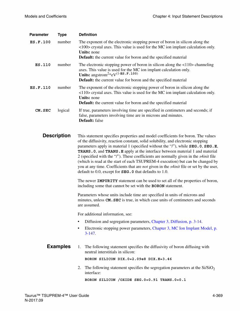
Models and Coefficients Chapter 4: Input Statement Descriptions

Description This statement specifies properties and model coefficients for boron. The values of the diffusivity, reaction constant, solid solubility, and electronic stopping parameters apply in material 1 (specified without the “/”), while SEG.0, SEG.E, TRANS.0, and TRANS.E apply at the interface between material 1 and material 2 (specified with the “/”). These coefficients are normally given in the s4init file (which is read at the start of each TSUPREM-4 execution) but can be changed by you at any time. Coefficients that are not given in the s4init file or set by the user, default to 0.0, except for SEG.0 that defaults to 1.0.

The newer IMPURITY statement can be used to set all of the properties of boron, including some that cannot be set with the BORON statement.

Parameters whose units include time are specified in units of microns and minutes, unless CM.SEC is true, in which case units of centimeters and seconds are assumed.

For additional information, see:

• Diffusion and segregation parameters, Chapter 3, Diffusion, p. 3-14.

• Electronic stopping power parameters, Chapter 3, MC Ion Implant Model, p. 3-147.

Examples 1. The following statement specifies the diffusivity of boron diffusing with neutral interstitials in silicon:

BORON SILICON DIX.0=2.09e8 DIX.E=3.46

2. The following statement specifies the segregation parameters at the Si/SiO2 interface:

BORON SILICON /OXIDE SEG.0=0.91 TRANS.0=0.1

ES.F.100 number The exponent of the electronic stopping power of boron in silicon along the <100> crystal axes. This value is used for the MC ion implant calculation only.Units: none Default: the current value for boron and the specified material

ES.110 number The electronic stopping power of boron in silicon along the <110> channeling axes. This value is used for the MC ion implant calculation only.Units: angstrom2*eV(1-ES.F.100) Default: the current value for boron and the specified material

ES.F.110 number The exponent of the electronic stopping power of boron in silicon along the <110> crystal axes. This value is used for the MC ion implant calculation only.Units: none Default: the current value for boron and the specified material

CM.SEC logical If true, parameters involving time are specified in centimeters and seconds; if false, parameters involving time are in microns and minutes. Default: false

Parameter Type Definition

Taurus™ TSUPREM-4™ User Guide 4-369N-2017.09

Chapter 4: Input Statement Descriptions Models and Coefficients

The concentration in silicon is 0.91 times the concentration in oxide, at equilibrium.

AdditionalBORON Notes

1. The BORON statement has been made obsolete by the IMPURITY statement, but remains available for compatibility with existing input files. Note that some properties of boron can only be set on the IMPURITY statement.

2. The fractional interstitial parameter FI that was used in TSUPREM-4 before Version 6.0 is no longer supported. Instead, it is now necessary to specify the diffusivities with interstitials and vacancies separately.

4-370 Taurus™ TSUPREM-4™ User GuideN-2017.09

Models and Coefficients Chapter 4: Input Statement Descriptions

PHOSPHORUS

The PHOSPHORUS statement sets some of the properties of phosphorus.

PHOSPHORUS {MATERIAL=<c> | SILICON | OXIDE | OXYNITRI | NITRIDE | POLYSILI | AMBIENT} [DIX.0=<n>] [DIX.E=<n>] [DIM.0=<n>] [DIM.E=<n>] [DIMM.0=<n>] [DIMM.E=<n>] [DVX.0=<n>] [DVX.E=<n>] [DVM.0=<n>] [DVM.E=<n>] [DVMM.0=<n>] [DVMM.E=<n>] [DIPAIR.0=<n>] [DIPAIR.E=<n>] [DVPAIR.0=<n>] [DVPAIR.E=<n>] [R.I.S=<n>] [E.I.S=<n>] [R.V.S=<n>] [E.V.S=<n>] [R.IP.V=<n>] [E.IP.V=<n>] [R.VP.I=<n>] [E.VP.I=<n>]

[ { IP.V.LOW | IP.V.MED | IP.V.HIG } ][ { VP.I.LOW | VP.I.MED | VP.I.HIG } ]

[SS.CLEAR] [SS.TEMP=<n> SS.CONC=<n>] [ {/MATERIA=<c> | /SILICON | /OXIDE | /OXYNITR | /NITRIDE | /POLYSIL | /AMBIENT} [SEG.0=<n>] [SEG.E=<n>] [TRANS.0=<n>] [TRANS.E=<n>]

[KSIP.0=<n>] [KSIP.E=<n>] [KSVP.0=<n>] [KSVP.E=<n>] ] [ES.RAND=<n> [ES.F.RAN=<n>]] [ES.100=<n> [ES.F.100=<n>]] [ES.110=<n> [ES.F.110=<n>]] [CM.SEC]

Parameter Type Definition

MATERIAL character The name of the material to which the other parameters apply (material 1 for the segregation terms).Default: none

SILICON logical Specifies that other parameters in this statement apply to phosphorus in silicon, and that silicon is material 1 for the segregation terms. Default: True if no other first material is specified

OXIDE logical Specifies that other parameters in this statement apply to phosphorus in oxide, and that oxide is material 1 for the segregation terms. Default: false

OXYNITRI logical Specifies that other parameters in this statement apply to phosphorus in oxynitride, and that oxynitride is material 1 for the segregation terms. Default: false

NITRIDE logical Specifies that other parameters in this statement apply to phosphorus in nitride, and that nitride is material 1 for the segregation terms. Default: false

POLYSILI logical Specifies that other parameters in this statement apply to phosphorus in polysilicon, and that polysilicon is material 1 for the segregation terms. Default: false

Taurus™ TSUPREM-4™ User Guide 4-371N-2017.09

Chapter 4: Input Statement Descriptions Models and Coefficients

AMBIENT logical Specifies that the ambient gas is material 1 for the segregation terms. Default: false Synonym: GAS

DIX.0 number The pre-exponential constant for diffusion of phosphorus with neutral interstitials. Units: microns2/min or cm2/s Default: the current value for this material

DIX.E number The activation energy for diffusion of phosphorus with neutral interstitials. Units: electron volts Default: the current value for this material

DIM.0 number The pre-exponential constant for diffusion of phosphorus with singly-negative interstitials. Units: microns2/min or cm2/s Default: the current value for this material

DIM.E number The activation energy for diffusion of phosphorus with singly-negative interstitials. Units: electron volts Default: the current value for this material

DIMM.0 number The pre-exponential constant for diffusion of phosphorus with doubly-negative interstitials. Units: microns2/min or cm2/s Default: the current value for this material

DIMM.E number The activation energy for diffusion of phosphorus with doubly-negative interstitials. Units: electron volts Default: the current value for this material

DVX.0 number The pre-exponential constant for diffusion of phosphorus with neutral vacancies. Units: microns2/min or cm2/s Default: the current value for this material

DVX.E number The activation energy for diffusion of phosphorus with neutral vacancies. Units: electron volts Default: the current value for this material

DVM.0 number The pre-exponential constant for diffusion of phosphorus with singly-negative vacancies. Units: microns2/min or cm2/s Default: the current value for this material

DVM.E number The activation energy for diffusion of phosphorus with singly-negative vacancies. Units: electron volts Default: the current value for this material

Parameter Type Definition

4-372 Taurus™ TSUPREM-4™ User GuideN-2017.09

Models and Coefficients Chapter 4: Input Statement Descriptions

DVMM.0 number The pre-exponential constant for diffusion of phosphorus with doubly-negative vacancies. Units: microns2/min or cm2/s Default: the current value for this material

DVMM.E number The activation energy for diffusion of phosphorus with doubly-negative vacancies. Units: electron volts Default: the current value for this material

DIPAIR.0 number The pre-exponential constant for the diffusivity of phosphorus-interstitial pairs. Units: microns2/min or cm2/s Default: the current value for this material

DIPAIR.E number The activation energy for the diffusivity of phosphorus-interstitial pairs.Units: electron volts Default: the current value for this material

DVPAIR.0 number The pre-exponential constant for the diffusivity of phosphorus-vacancy pairs. Units: microns2/min or cm2/s Default: the current value for this material

DVPAIR.E number The activation energy for the diffusivity of phosphorus-vacancy pairs.Units: electron volts Default: the current value for this material

R.I.S number The capture radius for the reaction between interstitials and substitutional phosphorus atoms.Units: ÅDefault: the current value for this material

E.I.S number The barrier energy for the reaction between interstitials and substitutional phosphorus atoms.Units: electron voltsDefault: the current value for this material

R.V.S number The capture radius for the reaction between vacancies and substitutional phosphorus atoms.Units: ÅDefault: the current value for this material

E.V.S number The barrier energy for the reaction between vacancies and substitutional phosphorus atoms.Units: electron voltsDefault: the current value for this material

R.IP.V number The capture radius for the reaction between phosphorus-interstitial pairs and vacancies.Units: ÅDefault: the current value for this material

Parameter Type Definition

Taurus™ TSUPREM-4™ User Guide 4-373N-2017.09

Chapter 4: Input Statement Descriptions Models and Coefficients

E.IP.V number The barrier energy for the reaction between phosphorus-interstitial pairs and vacancies.Units: electron voltsDefault: the current value for this material

R.VP.I number The capture radius for the reaction between phosphorus-vacancy pairs and interstitials.Units: ÅDefault: the current value for this material

E.VP.I number The barrier energy for the reaction between phosphorus-vacancy pairs and interstitials.Units: electron voltsDefault: the current value for this material

IP.V.LOW logical Assumes that only dopant-interstitial pairs and vacancies having opposite charges of equal magnitude react in bulk material.Default: true

IP.V.MED logical Assume that uncharged dopant-interstitial pairs (or vacancies) can react with vacancies (or dopant-interstitial pairs) in any charged state, and that oppositely charged dopant-interstitial pairs and vacancies can react.Default: false

IP.V.HIG logical Assumes that dopant-vacancy pairs in any charged state can react with interstitials in any charged state.Default: false

VP.I.LOW logical Assumes that only dopant-vacancy pairs and interstitials having opposite charges of equal magnitude react in bulk material.Default: true

VP.I.MED logical Assumes that uncharged dopant-vacancy pairs (or interstitials) can react with interstitials (or dopant-vacancy pairs) in any charged state, and that oppositely charged dopant-vacancy pairs and interstitials can react.Default: false

VP.I.HIG logical Assumes that dopant-vacancy pairs in any charged state can react with interstitials in any charged state.Default: false

SS.CLEAR logical Clears the solid solubility versus temperature table. Default: false

SS.TEMP number The temperature at which the solid solubility in material 1 is SS.CONC. Units: degrees Celsius Default: none

SS.CONC number The solid solubility in material 1 at temperature SS.TEMP. Units: atoms/cm3 Default: none

/MATERIA character The name of material 2 for the segregation parameters.Default: none

Parameter Type Definition

4-374 Taurus™ TSUPREM-4™ User GuideN-2017.09

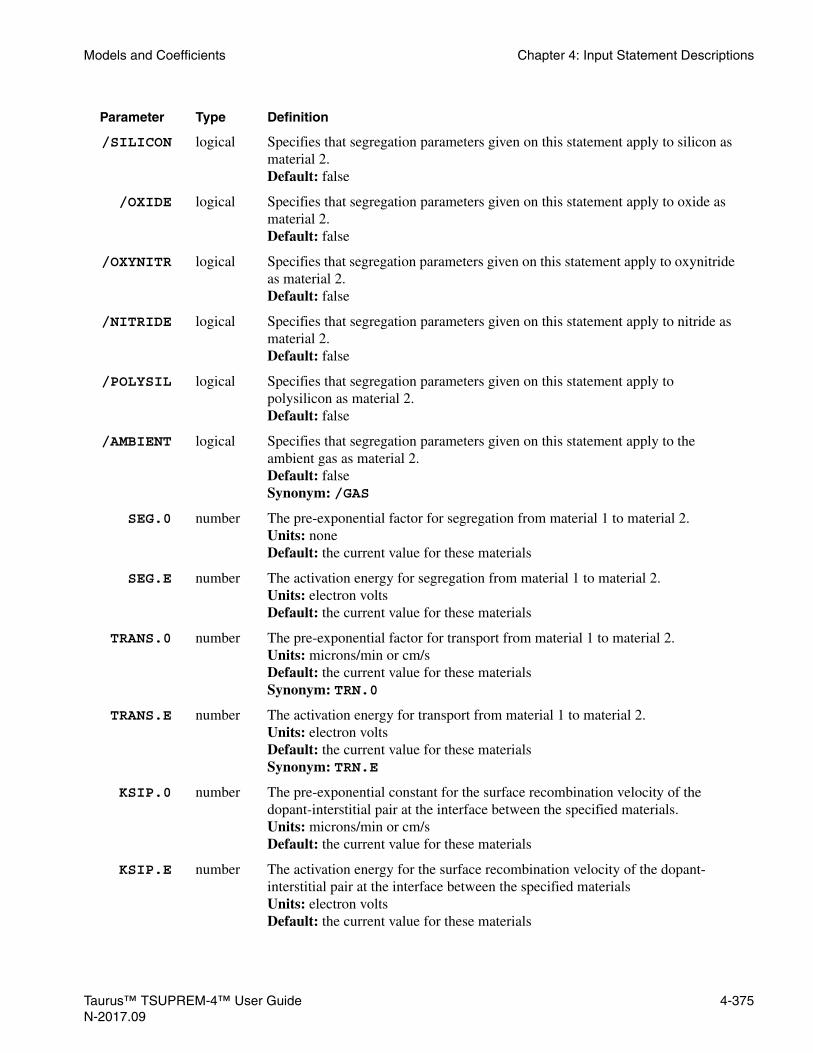
Models and Coefficients Chapter 4: Input Statement Descriptions

/SILICON logical Specifies that segregation parameters given on this statement apply to silicon as material 2. Default: false

/OXIDE logical Specifies that segregation parameters given on this statement apply to oxide as material 2. Default: false

/OXYNITR logical Specifies that segregation parameters given on this statement apply to oxynitride as material 2. Default: false

/NITRIDE logical Specifies that segregation parameters given on this statement apply to nitride as material 2. Default: false

/POLYSIL logical Specifies that segregation parameters given on this statement apply to polysilicon as material 2. Default: false

/AMBIENT logical Specifies that segregation parameters given on this statement apply to the ambient gas as material 2. Default: false Synonym: /GAS

SEG.0 number The pre-exponential factor for segregation from material 1 to material 2. Units: none Default: the current value for these materials

SEG.E number The activation energy for segregation from material 1 to material 2. Units: electron volts Default: the current value for these materials

TRANS.0 number The pre-exponential factor for transport from material 1 to material 2.Units: microns/min or cm/s Default: the current value for these materials Synonym: TRN.0

TRANS.E number The activation energy for transport from material 1 to material 2. Units: electron volts Default: the current value for these materials Synonym: TRN.E

KSIP.0 number The pre-exponential constant for the surface recombination velocity of the dopant-interstitial pair at the interface between the specified materials.Units: microns/min or cm/sDefault: the current value for these materials

KSIP.E number The activation energy for the surface recombination velocity of the dopant-interstitial pair at the interface between the specified materialsUnits: electron voltsDefault: the current value for these materials

Parameter Type Definition

Taurus™ TSUPREM-4™ User Guide 4-375N-2017.09

Chapter 4: Input Statement Descriptions Models and Coefficients

Description This statement specifies properties and model coefficients for phosphorus. The values of the diffusivity, reaction constant, solid solubility, and electronic stopping parameters apply in material 1 (specified without the “/”), while SEG.0, SEG.E, TRANS.0, and TRANS.E apply at the interface between material 1 and material 2 (specified with the “/”). These coefficients are normally given in the s4init file

KSVP.0 number The pre-exponential constant for the surface recombination velocity of the dopant-vacancy pair at the interface between the specified materials.Units: microns/min or cm/sDefault: the current value for these materials

KSVP.E number The activation energy for the surface recombination velocity of the dopant-vacancy pair at the interface between the specified materialsUnits: electron voltsDefault: the current value for these materials

ES.RAND number The electronic stopping power coefficient of implanted phosphorus in the specified material for materials other than silicon and for a nonchanneled direction in silicon. This value is used for the MC ion implant calculation only.Units: angstrom2*eV(1-ES.F.RAN) Default: the current value for phosphorus and the specified material

ES.F.RAN number The exponent of the electronic stopping power of implanted phosphorus in the specified material for materials other than silicon and for a nonchanneled direction in silicon. This value is used for the MC ion implant calculation only.Units: none Default: the current value for phosphorus and the specified material

ES.100 number The electronic stopping power of phosphorus in silicon along the <100> channeling axes. This value is used for the MC ion implant calculation only.Units: angstrom2*eV(1-ES.F.100) Default: the current value for phosphorus and the specified material

ES.F.100 number The exponent of the electronic stopping power of phosphorus in silicon along the <100> crystal axes. This value is used for the MC ion implant calculation only.Units: none Default: the current value for phosphorus and the specified material

ES.110 number The electronic stopping power of phosphorus in silicon along the <110> channeling axes. This value is used for the MC ion implant calculation only.Units: angstrom2*eV(1-ES.F.100) Default: the current value for phosphorus and the specified material

ES.F.110 number The exponent of the electronic stopping power of phosphorus in silicon along the <110> crystal axes. This value is used for the MC ion implant calculation only.Units: none Default: the current value for phosphorus and the specified material

CM.SEC logical If true, parameters involving time are specified in centimeters and seconds; if false, parameters involving time are in microns and minutes. Default: false

Parameter Type Definition

4-376 Taurus™ TSUPREM-4™ User GuideN-2017.09

Models and Coefficients Chapter 4: Input Statement Descriptions

(which is read at the start of each TSUPREM-4 execution) but can be changed by you at any time. Coefficients that are not given in the s4init file or set by the user, default to 0.0, except for SEG.0 that defaults to 1.0.

The newer IMPURITY statement can be used to set all of the properties of phosphorus, including some that cannot be set with the PHOSPHOR statement.

Parameters whose units include time are specified in units of microns and minutes, unless CM.SEC is true, in which case units of centimeters and seconds are assumed.

For additional information, see:

• Chapter 3, Diffusion, p. 3-14 for diffusion and segregation parameters.

• Chapter 3, MC Ion Implant Model, p. 3-147 for electronic stopping power parameters.

Examples 1. The following statement specifies the diffusion of phosphorus diffusing with doubly-negative interstitials in silicon:

PHOSPHORUS SILICON DIMM.0=2.652e11 DIMM.E=4.37

2. The following statement specifies the segregation parameters at the Si/SiO2 interface:

PHOS SILICON /OXIDE SEG.0=30.0 TRANS.0=0.1

The concentration in silicon is 30.0 times the concentration in oxide, at equilibrium.

AdditionalPHOSPHORUS

Notes

1. The PHOSPHORUS statement has been made obsolete by the IMPURITY statement, but remains available for compatibility with existing input files. Note that some properties of phosphorus can only be set on the IMPURITY statement.

2. The fractional interstitial parameter FI that was used in TSUPREM-4 before Version 6.0 is no longer supported. Instead, it is now necessary to specify the diffusivities with interstitials and vacancies separately.

Taurus™ TSUPREM-4™ User Guide 4-377N-2017.09

Chapter 4: Input Statement Descriptions Models and Coefficients

4-378 Taurus™ TSUPREM-4™ User GuideN-2017.09

CHAPTER 5

TN

Tutorial Examples5

This chapter presents three short examples showing how to use TSUPREM-4 to do some simple simulations. New users may wish to study these examples in sequence. Each example introduces new TSUPREM-4 commands and concepts. The examples in this chapter are fairly short and execute relatively quickly. The simulations presented in Chapter 6, Advanced Examples are more typical of real-life applications, and take more execution time. The examples include:

• 1-D Bipolar Example: a 1-D simulation of a bipolar transistor structure. This example illustrates the basic simulation steps using a simple 1-D grid.

• Local Oxidation: an example that shows how to set up a 2-D grid and how to activate the various oxidation and point defect models.

• Point Defect Models: an example illustrating the effect of the point defect models on impurity diffusion.

This chapter uses lowercase file names with the .inp extension for the example input files. Note the following regarding the format of input files:

• Each statement occupies one line, unless the statement is explicitly continued with a “+” character at the end of a line.

• Statement and parameter names can be abbreviated.

• On most statements, parameters can appear in any order.

• Blank lines between statements and extra spaces between parameters are ignored.

• Comment statements begin with the $ character and are used to document the input file.

• The input can contain a mixture of upper and lower case; the case is ignored, except in some character strings.

aurus™ TSUPREM-4™ User Guide 5-1-2017.09

Chapter 5: Tutorial Examples 1-D Bipolar Example

1-D Bipolar ExampleThis section presents a 1-D simulation of a bipolar transistor structure. The example simulates the active region of an oxide-isolated bipolar structure, from the buried collector region up through the emitter. The statements that direct the simulation are contained in the simulation input files s4ex1a.inp and s4ex1b.inp.

This example illustrates the mechanics of using TSUPREM-4 and the use of particular statements for mesh setup, model specification, simulation of processing steps, and printing and plotting of results. A 1-D example is presented primarily to simplify the discussion, but it also serves to illustrate a useful technique for performing fast simulations of simple structures.

TSUPREM-4 Input File Sequence

This example illustrates the organization of a typical TSUPREM-4 input file. In general, the sequence is as follows:

1. Identify the problem with comments, and set any necessary execution options (none are needed in most cases).

2. Generate an initial mesh, or read in a previously saved structure.

3. Simulate the desired process sequence, and print and/or plot the results.

Note that there is considerable flexibility in this sequence; for example, alternating between simulation and plotting. The only strict requirement is that a mesh must be defined before any processing or output can be performed.

5-2 Taurus™ TSUPREM-4™ User GuideN-2017.09

1-D Bipolar Example Chapter 5: Tutorial Examples

Initial Active Region Simulation

The input statements in the file s4ex1a.inp simulate the initial steps in the formation of the active region of a bipolar structure, including the formation of the buried collector and deposition of the epitaxial layer. These input statements are shown in Figure 5-1.

Figure 5-1 Input file s4ex1a.inp, for simulating the buried layer and epitaxial deposition for a bipolar transistor structure

$ TSUPREM-4 -- Example 1, Part A$ Bipolar active device region: Buried layer and epitaxial deposition

$ Use automatic grid generation and adaptive gridINITIALIZE BORON=1E15

$ Grow buried layer masking oxideDIFFUSION TEMP=1150 TIME=120 STEAM

$ Etch the buried layer masking oxideETCH OXIDE ALL

$ Implant and drive in the antimony buried layerIMPLANT ANTIMONY DOSE=1E15 ENERGY=75DIFFUSION TEMP=1150 TIME=30 DRYO2DIFFUSION TEMP=1150 TIME=360

$ Etch the oxide.ETCH OXIDE ALL

$ Grow 1.8 micron of arsenic-doped epitaxyEPITAXY THICKNES=1.8 SPACES=9 TEMP=1050 TIME=6 ARSENIC=5E15

$ Grow pad oxide and deposit nitrideDIFFUSION TEMP=1050 TIME=30 DRYO2DEPOSITION NITRIDE THICKNES=0.12

$ Save initial active region resultsSAVEFILE OUT.FILE=S4EX1AS

$ Plot resultsSELECT Z=LOG10(BORON) TITLE=”Active, Epitaxy” LABEL=LOG(CONCENTRATION)PLOT.1D BOTTOM=13 TOP=21 RIGHT=5 LINE.TYP=5 COLOR=2SELECT Z=LOG10(ARSENIC)PLOT.1D ^AXES ^C?LEAR LINE.TYP=2 COLOR=3SELECT Z=LOG10(ANTIMONY)PLOT.1D ^AX ^CL LINE.TYP=3 COLOR=3

$ Label plotLABEL X=4.2 Y=15.1 LABEL=BoronLABEL X=-.8 Y=15.8 LABEL=ArsenicLABEL X=2.1 Y=18.2 LABEL=Antimony

$ Print layer informationSELECT Z=DOPING

Taurus™ TSUPREM-4™ User Guide 5-3N-2017.09

Chapter 5: Tutorial Examples 1-D Bipolar Example

Mesh Generation

Traditionally, generation of the simulation mesh has been one of the most difficult and time-consuming tasks required for process simulation. If the mesh is too coarse, accuracy of the simulation is poor, while making the mesh too fine wastes time and computational resources. TSUPREM-4 simplifies the problem of creating an appropriate mesh by providing automatic mesh generation and adaptive gridding.Automatic Mesh Generation

A mesh is generated automatically when the INITIALIZE statement is processed. A boron concentration of 1015/cm3 for the initial structure has been specified. By default, the mesh that has two vertical lines, one at x=0 and one at x=1 micron. (For a 2-D simulation it would also be necessary to specify the width of the initial structure.) The location of the horizontal grid lines is determined by defaults set in the s4init file. The mesh can be made finer or coarser by including a MESH statement with the GRID.FAC parameter; the default spacing has been chosen for this example.

AdaptiveGridding

Adaptive gridding is done whenever an ion implantation or diffusion step is simulated to ensure that the grid is fine enough to maintain the required accuracy. The accuracy criteria can be adjusted with the ERR.FAC parameter on the METHOD statement; in this example the default values are used. By using adaptive gridding, the need to predict the grid requirements of a simulation in advance is eliminated.

Model Selection

The choice of simulation models should be considered before performing any processing steps. The speed and accuracy of the simulation depends strongly on the choice of models. The default models have been carefully chosen to give the best results in many cases, but some choices depend on the structures being simulated and on individual requirements of the user.

Two model choices must be made in most simulations:

• Oxidation model

• Point defect model

These selections are made using the METHOD statement. In this example the default models are used, that is, the VERTICAL oxidation model and the PD.FERMI point defect model.

The choice of models may be changed during the course of the simulation.

Oxidation Model The VERTICAL oxidation model can be used in this case because the simulation is one-dimensional, so only planar surfaces are oxidized. The ERFC oxidation model could also be used in this example, but it does not model the dependence of the oxidation rate on the concentration of impurities in the silicon. Also, the ERFC

5-4 Taurus™ TSUPREM-4™ User GuideN-2017.09

1-D Bipolar Example Chapter 5: Tutorial Examples

model requires an additional statement (an AMBIENT statement with the INITIAL parameter) to specify the initial oxide thickness whenever a structure with an initial oxide layer is oxidized, and does not automatically recognize the presence of nitride masking layers.

Point DefectModel

For this example the default point defect model (PD.FERMI) is used. The PD.TRANS point defect model increases the simulation time significantly, and should be used only when required. In this example, the effects of nonequilibrium point defect concentrations are relatively small. The magnitude of the error can be checked by repeating the simulation using the PD.TRANS or PD.FULL model.

Processing Steps

The following processing steps are used:

1. Buried layer masking oxide growth and patterning

2. Buried layer implant and drive-in

3. Epitaxial layer growth

4. Pad oxide growth and nitride mask deposition

Buried LayerMasking Oxide

The first step in the process is to grow an oxide to mask the buried layer implant. Oxidation is accomplished by specifying an oxidizing ambient (STEAM, in this case) on the DIFFUSION statement. The time (in minutes) and temperature(in °Celsius) must be specified. Note that specifying an oxidizing ambient turns on oxidation, but does not disable any other aspects of a diffusion step. Impurity diffusion and segregation at interfaces still occur.

The oxide must be removed from the active region of the device before implanting the buried layer. This is accomplished with the ETCH statement. The simplest form of the ETCH statement, used here, removes all of a specified material. The ETCH statement can also be used to remove portions of a layer.

Buried Layer The next step is to implant the buried layer and drive it in. This is done with the IMPLANT statement and the following DIFFUSION statements. The IMPLANT statement specifies the type of impurity, and the dose (per cm2) and energy (in keV). Use of adaptive gridding is generally sufficient to ensure that the mesh at the surface is fine enough to contain several grid points within the peak of the implanted distribution, but it is wise to plot the as-implanted distribution if there is any doubt.

The drive-in of the buried layer is done in two steps. In the first, a DRYO2 ambient is used to grow a thin layer of oxide to prevent outdiffusion of the implanted antimony. No ambient is given for the second; the absence of an ambient specification implies that an inert ambient is used. Once the drive-in is finished, the oxide is removed with an ETCH statement.

Taurus™ TSUPREM-4™ User Guide 5-5N-2017.09

Chapter 5: Tutorial Examples 1-D Bipolar Example

Epitaxial Layer Next, an epitaxial layer is grown. Epitaxial growth is simulated with the EPITAXY statement, which combines the effects of the DEPOSITION and DIFFUSION statements. The thickness of the deposited layer is specified to be 1.8 microns using the THICKNES parameter.

The grid density in the layer is determined by the SPACES parameter. This example specifies that 9 grid spaces be placed in the epitaxial layer. This produces a reasonable starting grid for the base and emitter processing that follows. Note that the specification of the number of spaces determines not only the grid in the resulting structure, but also the time discretization of the epitaxy step. The EPITAXY statement causes the deposition of one grid layer followed by a diffusion for some fraction of the total time. This process is repeated for each grid layer. If SPACES is not specified, its value defaults to one and the EPITAXY is equivalent to a DEPOSITION followed by a DIFFUSION statement.

The time and temperature for the epitaxial growth step are given by the TIME and TEMPERAT parameters, respectively. These determine the amount of diffusion that occurs during the growth process. The doping of the epitaxial layer can be specified with the ARSNIC parameter on the EPITAXY statement.

Pad Oxide andNitride Mask

Next, a pad oxide is grown (using the DIFFUSION statement with the DRYO2 parameter) and a nitride mask is deposited to be used for the field-isolation oxidation. The deposition is specified by the DEPOSITION statement, which specifies the material to deposit and the thickness of the layer. Other optional parameters can be used to specify the number and spacing of grid spaces in the deposited layer; by default, a single grid space is used in the deposited layer.

Saving the Structure

The resulting structure is saved using the SAVEFILE statement. In this case, it is saved in the output file named S4EX1AS. The saved structure is used as the starting point for the remaining process steps, which is simulated with a separate TSUPREM-4 input file.

It is recommended that the structure be saved after any long (in terms of computer time) sequence of operations. This allows the simulation to be resumed at that point should the need arise. It is also a good idea to save the structure at the end of any simulation, so that the results can be examined further at a later time.

Plotting the Results

The results of the simulation to this point are now ready to be displayed. This example demonstrates the use of the SELECT, PLOT.1D, and LABEL statements; 2-D plots are demonstrated in the next section.

5-6 Taurus™ TSUPREM-4™ User GuideN-2017.09

1-D Bipolar Example Chapter 5: Tutorial Examples

Specifying aGraphics Device

Before displaying a plot, the program must be told what sort of graphics device is being used. This can be done either with the DEVICE parameter on the OPTION statement or by using a default plot device. In this example, the default plot device is used. See , Chapter 4, on page 4-1 and Appendix AB.

The SELECTStatement

The value to be plotted is given by the Z expression on the SELECT statement. Z defines a mathematical expression that may contain a number of variables, functions, and mathematical operators. (See the description of the SELECT statement in Chapter 4, SELECT, p. 4-151). This example plots the base-10 logarithm of the various impurity concentrations.

Note:The Z expression is evaluated when the SELECT statement is processed. Thus the SELECT statement should be specified after any process steps that affect the device structure or solution quantities (for example, impurity concentrations) used in the expression.

The SELECT statement can also be used to specify a title for the plot and/or the label to be used on the vertical axis. If no label is given, the Z expression is used.

The PLOT.1DStatement

The PLOT.1D statement plots the values of a quantity along a (one-dimensional) section through the device. The section can be a vertical line at the location specified by X.VALUE, a horizontal line at Y.VALUE, or along an interface between two materials. This default is to plot along the vertical line at x=0.

The first PLOT.1D statement in this example plots the axes and title as well as the logarithm of the antimony concentration. In addition to the x coordinate, the minimum and maximum values for the y axis and the maximum value for the x axis have also been specified.

Note:The limits of the y axis are in the units of the Z expression on the SELECT statement; thus, 13 and 21 are used, (not 1e13 and 1e21).

If no axis limits are given, default values based on the dimensions of the device and the values of the Z expression are used.

By default, a dashed vertical line is drawn at the interfaces between materials. LINE.TYP=5 specifies that dashed line type 5 is to be used for plotting the boron profile; COLOR=2 specifies that color 2 (usually red) is to be used on color graphics devices.

The next two PLOT.1D statements add to the first plot. They do this by including the ^CLEAR and ^AXES specifications to prevent clearing of the screen and drawing of new axes, respectively. For each plot a new quantity to be plotted is specified (using a SELECT statement) along with a different line type and color.

Taurus™ TSUPREM-4™ User Guide 5-7N-2017.09

Chapter 5: Tutorial Examples 1-D Bipolar Example

Labels Labels are added to the plot with LABEL statements. Each LABEL statement specifies a text string to be plotted and a pair of x and y coordinates. The text string is plotted starting at the specified coordinates. X and Y are in the units of the plot axes, in this case microns and log10 (concentration), respectively. X and Y could also be given in centimeters, using the CM parameter. The final plot is shown in Figure 5-2.

Printing Layer Information

Although plots are the primary means of examining the results of a TSUPREM-4 simulation, useful information is also available from the PRINT.1D statement.

The PRINT.1DStatement

The PRINT.1D statement works with the Z expression given by a SELECT statement. Information is presented along a 1-D section specified in the same manner as in the PLOT.1D statement.

Three kinds of information can be printed:

1. A complete list of the values of the Z expression along the section.

2. The integral of the Z expression through each layer along the section.

3. The locations along the section where the Z expression has a specified value.

Figure 5-2 Impurity distributions in bipolar structure at end of input file s4ex1a.inp

Active, Epitaxy

0.00 2.00 4.00Distance (µm)

21

20

19

18

17

16

15

14

13

log(

Con

cent

ratio

n)

Antimony

Arsenic

Boron

5-8 Taurus™ TSUPREM-4™ User GuideN-2017.09

1-D Bipolar Example Chapter 5: Tutorial Examples

Using PRINT.1DLAYERS

The PRINT.1D statement at the end of file s4ex1a.inp uses the LAYERS parameter to request the integral of the Z expression (net doping) along a vertical section at x=0. The resulting output is shown in Figure 5-3.

For purposes of PRINT.1D LAYERS, a layer is defined as a portion of the section in which the material does not change and the sign of the Z expression is constant. In the case of net doping, each material is separated into layers of net n-type or net p-type doping.

In this example, the PRINT.1D LAYERS statement provides a number of useful results. For each layer, the material type, the top and bottom coordinates of the layer, the thickness of the layer, and the integral of the selected quantity are printed. A number of useful values are evident, such as the oxide thickness(491 Å) and the depth of the buried layer/substrate junction (4.71 μm).

Note:SELECT statement is required before a PRINT.1D LAYERS statement is processed, but you can use SELECT Z=0 if all you want to know is the layer thicknesses or the coordinates of the material interfaces.

Completing the Active Region Simulation

The simulation is now completed with a separate execution of TSUPREM-4, using the input file s4ex1b.inp shown in Figure 5-4. This file follows the same outline as the first (initialize, select models, process, output), and most of the statements are of the types discussed previously. However, there are some differences as discussed in the following subsections.

$ Print layer informationSELECT Z=DOPINGPRINT.1D LAYERS** Printing along X.VALUE=0:

Num Material Top Bottom Thickness Integral 1 nitride -1.3820 -1.2525 0.1200 1.2000e+00 2 oxide -1.2620 -1.2031 0.0491 5.5423e+08 3 silicon -1.2129 3.4935 4.7108 1.4215e+15 4 silicon 3.4979 200.0000 196.5021 -1.9630e+13

Figure 5-3 Output listing from PRINT.1D command in file s4ex1a.inp

Taurus™ TSUPREM-4™ User Guide 5-9N-2017.09

Chapter 5: Tutorial Examples 1-D Bipolar Example

Reading a SavedStructure

The most important difference is that instead of generating a mesh, the saved structure saved by the previous simulation is read from the file S4EX1AS. This is accomplished with the IN.FILE parameter on the INITIALIZE statement. The saved file includes complete mesh and solution information.

The next step specifies any needed model specifications. Because the choices of oxidation and point defect models were saved in the structure file, they do not need to be specified again. Any different models could be specified at this step.

Figure 5-4 Listing of input file s4ex1b.inp, showing statements for simulating the field oxide, base, and emitter region processing for a bipolar transistor

$ TSUPREM-4 -- Example 1, Part B$ Bipolar active device region: Field oxide, base, and emitter

$ Read structureINITIALIZE IN.FILE=S4EX1AS

$ Grow the field oxideDIFFUSION TEMP=800 TIME=20 T.FINAL=1000DIFFUSION TEMP=1000 TIME=10 DRYO2 T.FINAL=1100 P.FINAL=5DIFFUSION TEMP=1100 TIME=50 STEAM PRESSURE=5DIFFUSION TEMP=1100 TIME=10 DRYO2 PRESSURE=5 P.FINAL=1DIFFUSION TEMP=1100 TIME=60 T.FINAL=800

$ Remove nitride and pad oxideETCH NITRIDE ALLETCH OXIDE ALL

$ Implant the boron baseIMPLANT BORON DOSE=2E13 ENERGY=100

$ Implant the phosphorus emitterIMPLANT PHOSPHORUS DOSE=1E15 ENERGY=50

$ Anneal to activate base and emitter regionsDIFFUSION TEMP=1000 TIME=12 DRYO2

$ Plot resultsSELECT Z=LOG10(BORON) TITLE=”Active Region” LABEL=LOG(CONCENTRATION)PLOT.1D BOTTOM=13 TOP=21 RIGHT=5 LINE.TYP=5 COLOR=2SELECT Z=LOG10(PHOSPHORUS)PLOT.1D ^AXES ^CLEAR LINE.TYP=4 COLOR=4SELECT Z=LOG10(ARSENIC)PLOT.1D ^AXES ^CLEAR LINE.TYP=2 COLOR=3SELECT Z=LOG10(ANTIMONY)PLOT.1D ^AXES ^CLEAR LINE.TYP=3 COLOR=3

$ Label the impuritiesLABEL X= 2.0 Y=15.1 LABEL=BoronLABEL X=-1.0 Y=19.5 LABEL=PhosphorusLABEL X= 0.3 Y=15.8 LABEL=ArsenicLABEL X= 2.0 Y=18.4 LABEL=Antimony

$ Print the layer informationSELECT Z=DOPINGPRINT.1D X.V=0 LAYERS

5-10 Taurus™ TSUPREM-4™ User GuideN-2017.09

1-D Bipolar Example Chapter 5: Tutorial Examples

Field Oxidation The next step in the process is to grow the field isolation oxide. Although the active region of the device is being simulated, and no oxide is grown because of the nitride mask, the field oxidation step is included to simulate the dopant redistribution that occurs during the step. The field oxidation step illustrates how temperature and pressure ramping are specified.

The temperature is first ramped from 800°C to 1000°C, over a time of 20 minutes. The TEMP parameter specifies the starting temperature, while the T.FINAL parameter gives the temperature at the end of the step. The next step starts at 1000°C in a dry oxygen ambient at one atmosphere, and ramps the temperature to 1100°C and the pressure to 5 atmospheres over a period of 10 minutes. The starting pressure is given by the PRESSURE parameter (not needed here because the default value of one atmosphere is used), and the final pressure is given by P.FINAL. Note that ramp rates could also have been specified in degrees/minute or atmospheres/minute, using the T.RATE and P.RATE parameters, respectively. The third diffusion step does a 50-minute oxidation in steam, at a pressure of 5 atmospheres. Steps 4 and 5 ramp down the pressure, then the temperature. The remaining process steps are similar to those performed in the first part. The nitride and oxide are removed, and the base and emitter are implanted.

Final Structure

The plotting and labeling of the profiles use the statements described previously. The final plot is shown in Figure 5-5.

Figure 5-5 Final profiles produced by input file s4ex1b.inp

Active Region

0.00 2.00 4.00Distance (µm)

21

20

19

18

17

16

15

14

13

log(

Con

cent

ratio

n) Antimony

Arsenic

Boron

Phosphorus

Taurus™ TSUPREM-4™ User Guide 5-11N-2017.09

Chapter 5: Tutorial Examples Local Oxidation

A PRINT.1D statement is used to print layer information for the final structure. The SELECT Z=DOPING statement specifies that integrals of net doping are to be calculated and that layers are defined by the sign of the doping.

From the printed output (Figure 5-6) a number of useful values can be extracted, such as the oxide thickness (255 Å), the thickness of the emitter region (0.28 μm), and the integrated doping in the base region (8.12x1012/cm3).

Local OxidationThis section presents an example of a 2-D simulation of a local oxidation process. The purpose of this example is to illustrate the 2-D simulation capabilities of TSUPREM-4, and to provide some practical hints on the effective use of these capabilities.

This example simulates a narrow, locally-oxidized isolation region. The two features of interest are the oxide thickness and shape and the impurity distribution in the underlying silicon. These are examined in separate simulations. The commands for performing the simulations are contained in the simulation input files s4ex2a.inp and s4ex2b.inp.

Calculation of Oxide Shape

The first goal of this simulation is to determine the effect of using a narrow mask opening on the oxide shape. The input statements for this simulation are shown in Figures 5-7 and 5-9. The steps are similar to those used in the previous example, but are complicated slightly by the 2-D nature of the simulation.

$ Print the layer informationSELECT Z=DOPINGPRINT.1D LAYERS** Printing along X.VALUE=0:

Num Material Top Bottom Thickness Integral 1 oxide -1.2281 -1.2025 0.0255 3.7599e+12 2 silicon -1.2025 -0.9202 0.2823 1.0427e+15 3 silicon -0.9202 -0.5746 0.3456 -8.1165e+12 4 silicon -0.5746 3.5837 4.1584 1.4212e+15 5 silicon 3.5837 200.0000 196.4136 -1.9623e+13

Figure 5-6 Output listing from PRINT.1D command in file s4ex1b.inp

5-12 Taurus™ TSUPREM-4™ User GuideN-2017.09

Local Oxidation Chapter 5: Tutorial Examples

$ TSUPREM-4 narrow window example$ Part 1: Oxide shape

$ Set up the gridLINE X LOC=0.0 SPAC=0.15LINE X LOC=1.25 SPAC=0.05LINE X LOC=1.5 SPAC=0.1

LINE Y LOC=0 SPAC=0.03LINE Y LOC=0.5 SPAC=0.1

$ No impurities, for faster oxidation simulationINITIALIZE

$ Deposit pad oxide and define nitride maskDEPOSITION OXIDE THICKNES=0.03 SPACES=2DEPOSITION NITRIDE THICKNES=0.10 SPACES=2ETCH NITRIDE RIGHT P1.X=1.25

$ Plot the gridSELECT TITLE="Grid for Oxidation"PLOT.2D GRID SCALE C.GRID=2

$ Do the oxidationMETHOD VISCOEL DY.OXIDE=0.05 INIT=0.15AMBIENT MAT=OXIDE VC=170AMBIENT MAT=NITRIDE VC=100DIFFUSION TEMP=1000 TIME=100 WETO2

$ Save the structureSAVEFILE OUT.FILE=S4EX2AS

Figure 5-7 First part of input file s4ex2a.inp, for determining LOCOS shape

Figure 5-8 Mesh used for oxidation simulation. Produced by PLOT.2D GRID statement in input file s4ex2a.inp

0.00 0.50 1.00 1.50Distance (µm)

Dis

tanc

e (µ

m)

0.50

0.00

Taurus™ TSUPREM-4™ User Guide 5-13N-2017.09

Chapter 5: Tutorial Examples Local Oxidation

Mesh Generation The simulation starts by defining a mesh. The object in this case is to define as coarse a mesh as possible without losing accuracy in the solution. (The accuracy can be checked later by repeating the simulation with a finer mesh.) Only half of the structure needs to be simulated, because of the symmetry of the structure. The LINE X statements specify the horizontal locations of vertical grid lines. The first and last LINE X statements specify the left and right edges of the structure; the SPACING parameters specify the horizontal grid spacings at these locations. Other LINE X statements are used to add grid lines and specify spacings at other locations in the structure. In the vertical direction, LINE Y statements specify the top and bottom locations (and corresponding grid spacings) for the mesh.

The grid for this example does not need to be very fine. In the horizontal direction the spacing is set to 0.05 microns at the edge of the nitride mask, where the 2-D effects are greatest (x=1.25); the spacing expands to 0.1 micron at the right edge and 0.15 micron at the left edge. In the vertical direction, the spacing is set to 0.03 at the top, expanding to 0.1 at the bottom.

The effect of the grid spacing on accuracy can be checked by running the simulation again with a finer mesh; this can be accomplished by adding a MESH statement with the GRID.FAC parameter anywhere before the INITIALIZE statement. There are no impurities specified in this simulation, so no adaptive gridding occurs based on implantation or diffusion of impurities. However, the grid is refined as needed based on oxidant concentration.

The INITIALIZE statement performs the actual mesh generation. Note that no substrate doping has been specified. This speeds up the simulation slightly by eliminating the need to solve for impurity diffusion while oxidizing.

Pad Oxide andNitride Layers

Next the pad oxide is deposited. To improve the accuracy when calculating oxidant diffusion in the oxide, two grid spaces are placed in the deposited layer. (When checking the accuracy of the simulation, more divisions would be useful.) More grid spaces are added automatically as the oxide grows.

To mask the oxidation, a nitride layer is deposited and then patterned with an ETCH statement. The RIGHT keyword on the ETCH statement specifies that material is to be etched to the right of the line defined by the P1.X, P1.Y, P2.X, and P2.Y parameters. P1.X=1.25 is specified; P1.Y defaults to a value above the highest point of the structure; P2.X defaults to the value of P1.X; and P2.Y defaults to a value below the bottom of the structure. Thus the etch occurs to the right of a vertical line through the structure at x=1.25 microns.

Plotting the Mesh At this point it is wise to inspect the mesh. This is done with the PLOT.2D statement. The PLOT.2D statement is used to set up any 2-D plot. By itself, it can plot the material boundaries of a structure, the grid, and oxide stress and velocity vectors. It is also used to set the scale and draw axes for contour plots. In this case, the GRID keyword requests that the grid be plotted, and the C.GRID keyword specifies the color to be used.

5-14 Taurus™ TSUPREM-4™ User GuideN-2017.09

Local Oxidation Chapter 5: Tutorial Examples

The SCALE parameter causes the x or y axis to be scaled to reflect the true aspect ratio of the structure. If SCALE had not been specified, the plot would be stretched in the y-direction to fill the plotting area.

The SELECT statement is used only to specify a title for the plot. The resulting plot is shown in Figure 5-8.

Model Selection Next a METHOD statement is used with the VISCOELA keyword to select the oxidation model. The VISCOELA model is used because it allows fast simulation of two-dimensional, stress-dependent oxidation. The DY.OXIDE parameter sets the grid spacing to be used in the growing oxide. (The same grid is used both for the diffusion of the oxidizing species and for the calculation of oxide movement.) The INIT.TIM parameter specifies an initial time step of 0.15 minutes; this saves a small amount of calculation time. The default value is 0.002 minutes, which is appropriate for many diffusion steps but smaller than necessary for oxidation-only steps.

The effects of oxidant diffusion, interface reaction rate, and material viscosities on the stresses in the structure are included by default. Because the models for the stress effects do not include the dependence of parameter values on temperature, it is necessary to use AMBIENT statements to specify appropriate values for VC (the dependence of stress on material viscosity) at the oxidation temperature. (Suitable values are listed in the notes to Appendix AA.)

The oxidation is accomplished by the DIFFUSION statement, which specifies a wet oxygen ambient at 1000°C for 100 minutes. The SAVEFILE statement saves the final structure for later analysis.

Taurus™ TSUPREM-4™ User Guide 5-15N-2017.09

Chapter 5: Tutorial Examples Local Oxidation

Plotting theResults

The results are plotted using the statements shown in Figure 5-9. The PLOT.2D statement is used to plot the structure boundaries and material interfaces. The following parameters specify the plot format and content:

• FLOW adds vectors showing the speed and direction of material flow in the structure due to oxidation.

• VLENG specifies the maximum length of a flow vector (in microns) to be plotted.

• The X.MIN parameter specifies the minimum value of the x axis: (X.MAX, Y.MIN, and Y.MAX can be used to specify the other axis limits, but the default values are used in this case).

• The SCALE parameter is used to avoid distorting the structure as it is scaled for plotting.

$ Plot the final structure, showing flow linesSELECT TITLE="Flow at End of Oxidation Step"PLOT.2D SCALE FLOW VLENG=0.065 X.MIN=0.5 C.FLOW=4

$ Plot the final structure, showing stress vectorsSELECT TITLE="Stresses After Oxidation"PLOT.2D SCALE STRESS VLENG=0.2 X.MIN=0.5 + C.COMPRE=4 C.TENSIO=2 L.TENSIO=2

$ Plot filled contours of hydrostatic pressureSELECT Z=( -0.5 * ( SXX + SYY ) ) TITLE="Contours of Hydrostatic Pressure"PLOT.2D SCALE X.MIN=0.5 X.MAX=1.8FOREACH I ( 1 TO 5 ) COLOR MIN.V=(( I - 0.5)*2E9) MAX.V=(( I + 0.5)*2E9) COLOR=(13 + I ) COLOR MIN.V=((- I - 0.5)*2E9) MAX.V=((- I + 0.5)*2E9) COLOR=(25 - I )END

$ Create a legendLABEL X=1.52 Y=-0.2 LABEL="Compression" SIZE=0.3LABEL X=1.60 Y=-0.15 LABEL="1-3E9" C.RECT=14 SIZE=0.3 W.RECT=0.35 H.R=0.35LABEL X=1.60 Y=-0.1 LABEL="3-5E9" C.RECT=15 SIZE=0.3 W.RECT=0.35 H.R=0.35LABEL X=1.60 Y=-0.05 LABEL="5-7E9" C.RECT=16 SIZE=0.3 W.RECT=0.35 H.R=0.35LABEL X=1.60 Y= 0.0 LABEL="7-9E9" C.RECT=17 SIZE=0.3 W.RECT=0.35 H.R=0.35LABEL X=1.52 Y= 0.05 LABEL="Tension" SIZE=0.3LABEL X=1.60 Y= 0.1 LABEL="1-3E9" C.RECT=24 SIZE=0.3 W.RECT=0.35 H.R=0.35LABEL X=1.60 Y= 0.15 LABEL="3-5E9" C.RECT=23 SIZE=0.3 W.RECT=0.35 H.R=0.35LABEL X=1.60 Y= 0.20 LABEL="5-7E9" C.RECT=22 SIZE=0.3 W.RECT=0.35 H.R=0.35LABEL X=1.60 Y= 0.25 LABEL="7-9E9" C.RECT=21 SIZE=0.3 W.RECT=0.35 H.R=0.35

$ Redraw boundariesPLOT.2D ^AX ^CL

$ Print location of interfaceSELECT Z=YPRINT.1D SILICON /OXIDE

Figure 5-9 Second part of statement input file s4ex2a.inp, showing statements for plotting results of LOCOS process

5-16 Taurus™ TSUPREM-4™ User GuideN-2017.09

Local Oxidation Chapter 5: Tutorial Examples

The result of the PLOT.2D FLOW statement is shown in Figure 5-10.

Plotting Stresses Stresses in the structure can be plotted in several ways. One way is to use the PLOT.2D statement with the STRESS parameter. The STRESS parameter requests that the principal components of stress be shown. The stresses are indicated by short lines whose lengths are proportional to the stress components. The line type indicates whether the material is in tension or compression. By default, both use line type one, but in this example LINE.TEN=2 is specified so that a dashed line is used to indicate tension (the default is one). Tension and compression are also distinguished by color, using the C.TENSIO and C.COMPRE parameters. The VLENG parameter specifies the length of the line (in the units of the plot axes, that is, microns) used for the maximum value of stress. Smaller stresses produce proportionally smaller lines.

The stress plot is shown in Figure 5-11. The long, solid lines indicate large compressive stresses in the direction of the lines; dashed lines indicate tension. As expected, the stresses are concentrated near the portion of the structure where the oxide growth is nonuniform and where the nitride is forced to bend.

Figure 5-10 Plot produced by the PLOT.2D FLOW statement in input file s4ex2a.inp

0.50 1.00 1.50Distance (µm)

Dis

tanc

e (µ

m)

0.25

-0.2

5

Flow at End of Oxidation Step

Taurus™ TSUPREM-4™ User Guide 5-17N-2017.09

Chapter 5: Tutorial Examples Local Oxidation

Contour Plots Another way to show the stresses in the structure is with contour plots. It is difficult to show all three components of stress in a contour plot, and it is not very useful to show individual components because of their dependence on the choice of coordinate system. However, meaningful combinations of the stresses can be calculated with the SELECT statement and plotted with the PLOT.2D and CONTOUR or COLOR statements.

This example shows how the hydrostatic pressure, defined as the negative average of the Sxx and Syy stress components, can be plotted.

• The SELECT statement simply gives the mathematical expression for the function to be plotted.

• The PLOT.2D statement plots the axes, structure boundaries, and material interfaces, X.MAX is specified greater than the right edge of the structure to leave room for a legend.

• A pair of COLOR statements inside a FOREACH loop are used to shade regions of differing pressures.

The FOREACH statement specifies a variable (I) and a range of values (1 to 5, in this case). The statements between the FOREACH statement and the matching END statement are executed once for each value of the variable.

Figure 5-11 Plot produced by the PLOT.2D STRESS statement in input file s4ex2a.inp

0.50 1.00 1.50Distance (µm)

Dis

tanc

e (µ

m)

0.25

-0.2

5

Stresses After Oxidation

5-18 Taurus™ TSUPREM-4™ User GuideN-2017.09

Local Oxidation Chapter 5: Tutorial Examples

The COLOR statements specify a color and the range of pressures to be represented by that color. Both the color and the minimum and maximum values are given by arithmetic expressions that depend on the variable I.

• A series of LABEL statements are used to produce a legend, showing the amount of tension or compression corresponding to each color.

Each LABEL statement specifies the location of the label (in microns, in this case), the text of the label, and a filled rectangle that is placed before the label. The size of the characters (in centimeters) is specified by the SIZE parameter. Width and height of the rectangle are given by W.RECTAN and H.RECTAN (abbreviated to W.R and H.R, respectively).

• Finally, a last PLOT.2D with the ^AXES and ^CLEAR parameters is done to redraw the structure boundaries, which may have been obscured when plotting the shaded contours. The result is shown in Figure 5-12.

The last two lines of s4ex2a.inp show how the y coordinate of the silicon/oxide interface can be printed as a function of x, using the PRINT.1D statements to print solution values along the interface between two materials.

2-D Diffusion With Point Defects

This example analyzes the diffusion of impurities during the local oxidation step. The same process is simulated as in the previous sections, except with boron in the substrate and a boron implant. The effects of point defect generation during oxidation are also included, but with a simpler oxidation model to reduce the computer time requirements. The listing of the input (from file s4ex2b.inp) is shown in Figures 5-13 and 5-15.

Figure 5-12 Contours of hydrostatic pressure plotted by statements in input file s4ex2a.inp

0.50 1.00 1.50Distance (µm)

Dis

tanc

e (µ

m)

0.25

-0.2

5

Compression1−3E93−5E95−7E97−9E9

1−3E93−5E95−7E97−9E9

Tension

Taurus™ TSUPREM-4™ User Guide 5-19N-2017.09

Chapter 5: Tutorial Examples Local Oxidation

Automatic GridGeneration

For convenience, automatic grid generation is used for this analysis. By specifying WIDTH=1.5 on the INITIALIZE statement, the grid extends from x=0 to x=1.5, just as in the previous simulation. The background concentration of the substrate is specified with the BORON parameter. The grid is automatically refined as needed to maintain the accuracy of the impurity profiles.

Field Implant The deposition of the pad oxide and nitride are the same as before. Now, however, a photoresist layer is deposited and patterned to be used as a boron implant mask. The boron is implanted through the pad oxide, then the photoresist is removed.

Oxidation The COMPRESS oxidation model is chosen to obtain a fast 2-D simulation. The 2-D point defect model is specified by the PD.TRANS keyword on the METHOD statement. The DIFFUSION statement is the same as in the previous section.

The structure is saved at the end of the simulation so the results can be examined further without rerunning the simulation. In this example, the solution is saved in the file S4EX2BS.

Figure 5-13 First part of input file s4ex2b.inp, showing processing steps

$ TSUPREM-4 narrow window example$ Part 2: Impurity distribution

$ Use default gridINITIALIZE BORON=1E15 WIDTH=1.5

$ Deposit pad oxide, LOCOS mask, and implant maskDEPOSITION OXIDE THICKNES=0.03 SPACES=2DEPOSITION NITRIDE THICKNES=0.10DEPOSITION PHOTO THICKNES=2

ETCH PHOTO RIGHT P1.X=1.25ETCH NITRIDE TRAP

$ Implant boronIMPLANT BORON DOSE=2E13 ENERGY=100ETCH PHOTORESIST ALL

$ Do the drive-in, with point defectsMETHOD COMPRESS PD.TRANSDIFFUSION TEMP=1000 TIME=100 WETO2

$ Save the structureSAVEFILE OUT.FILE=S4EX2BS

$ Plot the grid after diffusionSELECT TITLE=”Grid After Impurity Diffusion”PLOT.2D SCALE GRID Y.MAX=1.2 C.GRID=2

5-20 Taurus™ TSUPREM-4™ User GuideN-2017.09

Local Oxidation Chapter 5: Tutorial Examples

Grid Plot The grid at this point is plotted by the PLOT.2D GRID statement. The plot is shown in Figure 5-14. The grid has been refined near the surface and around the field isolation oxide to improve the resolution of the boron profile.

The Y.MAX parameter is used to restrict the plot to the upper part of the structure. If Y.MAX had been omitted, the entire grid would have been plotted down to the bottom of the structure (at y=200 microns) in its 1.5:200 aspect ratio, producing a nearly useless result. If the SCALE parameters had been omitted, the plot would be compressed in the y direction to make it fit the available plotting area, but the shape of the structure would be distorted.

The SELECT statement has been used to specify a title for the plot.

Contour of BoronConcentration

Figure 5-15 shows the input statements used to plot the results. The first plot shows contours of equal boron concentration. A PLOT.2D statement sets up the axes for the plot and draws the boundaries of the structure and the material interfaces. Y.MAX=1.2 (microns) is specified so that only the portion of the device near the surface is plotted. The SELECT statement specifies that the (base 10) logarithm of the boron concentration is to be plotted.

Figure 5-14 Grid plot produced by first PLOT.2D statement in input file s4ex2b.inp

0.50 1.00 1.50Distance (µm)

Dis

tanc

e (µ

m)

1.00

0.00

0.00

0.50

Grid After Impurity Diffusion

Taurus™ TSUPREM-4™ User Guide 5-21N-2017.09

Chapter 5: Tutorial Examples Local Oxidation

Figure 5-15 Second part of input file s4ex2b.inp, showing statements for plotting the results of the diffusion simulation

$ Plot contours of boronSELECT Z=LOG10(BORON) TITLE=”Contours of Boron Concentration”PLOT.2D SCALE Y.MAX=1.2FOREACH X (15.5 16.5 17) CONTOUR VAL=X COLOR=2ENDCONTOUR VAL=16 LINE.TYP=2 COLOR=2

$ Plot interstitials and vacancies vs. depthSELECT Z=INTER/CI.STAR TITLE=”Point Defects vs. Y (X=1.5)” + LABEL=”Normalized Defect Concentration”PLOT.1D X.VALUE=1.5 BOTTOM=-1 RIGHT=80.0 COLOR=4SELECT Z = VACAN/CV.STARPLOT.1D X.VALUE=1.5 ^AXES ^CLEAR LINE.TYP=2 COLOR=6

$ Label the plotLABEL X=5 Y=4.0 LABEL=InterstitialsLABEL X=4 Y=0.7 LABEL=Vacancies

$ Plot interstitials and vacancies vs. widthSELECT Z=INTER/CI.STAR TITLE=”Point Defects vs. X (Y=2um)” + LABEL=”Normalized Defect Concentration”PLOT.1D Y.VAL=2 BOTTOM=-1 COLOR=4SELECT Z=VACAN/CV.STARPLOT.1D Y.VAL=2 ^AX ^CL LINE.TYP=2 COLOR=6LABEL X=0.2 Y=4.5 LABEL=InterstitialsLABEL X=0.2 Y=0.5 LABEL=Vacancies

$ Prepare to plot contours of point defect concentrationsSELECT Z=INTER/CI.STAR TITLE=”Interstitial Contours”PLOT.2D SCALE Y.MAX=1.5 X.MAX=2.1

$ Plot contours of interstitialsFOREACH I ( 0 to 7 ) COLOR MIN.V=(( I -0.5)*1.0+1.5) MAX.V=(( I +0.5)*1.0+1.5) COLOR=(9 + I )END

$ Create a legendLABEL X=1.68 Y=0.15 LABEL=”I/I*:” SIZE=.3LABEL X=1.8 Y=0.30 LABEL=”1.5” SIZE=.3 W.RECT=.35 H.R=.35 C.R=9LABEL X=1.8 Y=0.45 LABEL=”2.5” SIZE=.3 W.RECT=.35 H.R=.35 C.R=10LABEL X=1.8 Y=0.60 LABEL=”3.5” SIZE=.3 W.RECT=.35 H.R=.35 C.R=11LABEL X=1.8 Y=0.75 LABEL=”4.5” SIZE=.3 W.RECT=.35 H.R=.35 C.R=12LABEL X=1.8 Y=0.90 LABEL=”5.5” SIZE=.3 W.RECT=.35 H.R=.35 C.R=13LABEL X=1.8 Y=1.05 LABEL=”6.5” SIZE=.3 W.RECT=.35 H.R=.35 C.R=14LABEL X=1.8 Y=1.20 LABEL=”7.5” SIZE=.3 W.RECT=.35 H.R=.35 C.R=15LABEL X=1.8 Y=1.35 LABEL=”8.5” SIZE=.3 W.RECT=.35 H.R=.35 C.R=16

$ Redraw the boundariesPLOT.2D ^AX ^CL

$ Label the plotLABEL X=1.4 Y= 0.0 LABEL=Oxide RIGHT

$ Print boron vs. depth in field regionSELECT Z=BORONPRINT.1D X.VALUE=0 X.MAX=2

5-22 Taurus™ TSUPREM-4™ User GuideN-2017.09

Local Oxidation Chapter 5: Tutorial Examples

The CONTOUR statement plots a contour at a single value of the selected quantity, so a series of CONTOUR statements is needed for a typical contour plot. The specification of these CONTOUR statements is simplified by using the FOREACH and END statements to define a loop.

Using theFOREACHStatement

The FOREACH statement is special in that it does not use the usual “parameter=value” type of syntax. Instead it requires a variable name followed by a list of values in parentheses. The variable name can have up to 8 characters and must start with a letter. The values in the list can be numbers or other syntactic items (for example, character strings) and must be separated by spaces. When the FOREACH loop is executed, each of the following statements up to the matching END statement is executed with the variable replaced by successive values from the FOREACH list wherever it occurs.

In this example the variable X takes on the values 15.5, 16.5, and 17. The variable X is used as the value of the VALUE parameter in the CONTOUR statement to generate a contour at each of the values listed in the FOREACH statement. The value 16 is purposely omitted from the list so that the contour could be drawn with a separate CONTOUR statement using LINE.TYP=2. Thus the contour for a boron concentration of 1016 is drawn with a dashed line to distinguish it from the other contours. The resulting plot is shown in Figure 5-16.

Figure 5-16 Contours of boron concentration produced by input file s4ex2b.inp

0.50 1.00 1.50Distance (µm)

Dis

tanc

e (µ

m)

1.00

0.00

0.00

0.50

Taurus™ TSUPREM-4™ User Guide 5-23N-2017.09

Chapter 5: Tutorial Examples Local Oxidation

VerticalDistribution ofPoint Defects

The distribution of interstitials and vacancies is examined next. By understanding the behavior of these point defects, more accurate and efficient simulations may be set up. It is usually most convenient to normalize the interstitial and vacancy concentration to their equilibrium values, since it is the normalized quantities that are used in the equations for impurity diffusion. Thus, in the SELECT statements, divide the interstitial and vacancy concentrations by CI.STAR and CV.STAR, the equilibrium concentrations for interstitials and vacancies, respectively.

The first PLOT.1D statement plots the distribution of interstitials along a vertical section at X.VALUE=0. The maximum value on the x axis (which corresponds to depth, in this case) is given by RIGHT. The minimum value on the y axis is set to -1 with the BOTTOM parameter. The normalized vacancy concentration is plotted on the same graph, using line type 2 and color 6. The LABEL statements help us to remember which curve is which on the plot.

The resulting plot, shown in Figure 5-17, reveals several interesting things about the point defect concentrations during oxidation:

• The point defect profiles extend to a much greater depth than the dopant profiles. Thus a deeper simulation structure is needed, although in this case a structure only 50 to 100 microns deep would have sufficed.

• The oxidation has produced a greatly enhanced interstitial concentration near the surface, and a greatly reduced vacancy concentration. The diffusivity of impurities that diffuse with interstitials (for example boron and phosphorus) is enhanced, while the diffusion of impurities that diffuse with vacancies is retarded (for example, antimony).

Figure 5-17 Concentration of point defects versus depth, as plotted by input file s4ex2b.inp

20.00 40.00 60.00

Distance (µm)

Nor

mal

ized

Def

ect C

once

ntra

tion

05

0.00

2.5

80.00

7.5

Interstitials

Vacancies

Point Defects versus Y (X=1.5)

5-24 Taurus™ TSUPREM-4™ User GuideN-2017.09

Local Oxidation Chapter 5: Tutorial Examples

LateralDistribution ofPoint Defects

The distribution of point defects across the width of the device is examined to determine how dense the horizontal grid must be deep in the structure. The next set of SELECT, PLOT.1D, and LABEL statements plot the point defect distributions across the width of the device at y=2 microns. The sequence of statements is the same as for the previous plot, except that Y.VALUE=2 has been specified on the PLOT.1D statements instead of X.VALUE=0. The results are shown in Figure 5-18.

Although visually uninteresting, this plot reveals a very important property of the point defect distributions—because point defects diffuse so rapidly, the point defect profiles deep in the structure are essentially one-dimensional. Thus it is possible to eliminate the vertical grid lines deep in the structure to reduce the simulation time.

Shaded Contoursof Interstitial

Concentration

Finally, shaded contours of interstitial concentrations are plotted. The procedure is the same as for plotting the boron contours. The axes and material boundaries are plotted with a PLOT.2D statement. In this case, Y.MAX=2 microns is used to plot a deeper section of the device. The SELECT statement is used to specify the normalized interstitial concentration as the plot quantity and to give a title for the plot.

Again, the general expression capability of the SELECT statement is used to scale the interstitial concentration by the equilibrium value (CI.STAR). A series of shaded contours are plotted, using the FOREACH, COLOR, and END statements. LABEL statements with shaded rectangles are used to create a legend for the plot. A final PLOT.2D with ^AXES and ^CLEAR is used to replot the boundaries of the structure. The final plot is shown in Figure 5-19.

Figure 5-18 Concentration of point defects versus width, as plotted by input file s4ex2b.inp

0.50 1.00Distance (µm)

Nor

mal

ized

Def

ect C

once

ntra

tion

05

0.00

2.5

1.50

7.5

Interstitials

Vacancies

Point Defects versus X (Y=2 µm)

Taurus™ TSUPREM-4™ User Guide 5-25N-2017.09

Chapter 5: Tutorial Examples Point Defect Models

Local Oxidation Summation

This section has shown how the shape of an isolation structure and the corresponding impurity profiles can be determined by separate simulations. In many cases this is the most efficient way to obtain an accurate simulation, because it allows the grids and solution methods to be optimized for each aspect of the problem. Adjustments to the process can be analyzed more quickly; often it is only necessary to repeat one of the simulations. As a final check, the two simulations could be combined, using a somewhat denser mesh. This solution would be more time-consuming, but a single simulation should suffice to verify the results obtained previously.

Point Defect ModelsThis example shows the differences in results using the three point defect models:

• The PD.FERMI model is the simplest point defect model; it is the fastest of the three, because it assumes that the point defect concentrations are at equilibrium and thus do not need to be calculated explicitly.

The PD.FERMI model does not simulate the effects of nonequilibrium point defect concentrations on impurities, nor the effects of impurities on point defect concentrations (except for the dependence on Fermi level).

Figure 5-19 Contours of interstitial concentration, as plotted by input file s4ex2b.inp

Oxide

1.00 2.00Distance (µm)

Dis

tanc

e (µ

m)

1.00

0.00

0.00

I / I*:1.5

2.5

3.5

4.5

5.5

6.5

7.5

8.5

5-26 Taurus™ TSUPREM-4™ User GuideN-2017.09

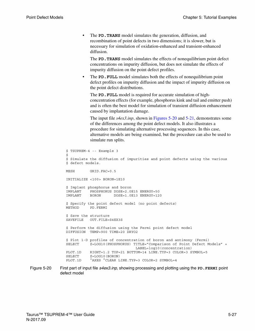
Point Defect Models Chapter 5: Tutorial Examples

• The PD.TRANS model simulates the generation, diffusion, and recombination of point defects in two dimensions; it is slower, but is necessary for simulation of oxidation-enhanced and transient-enhanced diffusion.

The PD.TRANS model simulates the effects of nonequilibrium point defect concentrations on impurity diffusion, but does not simulate the effects of impurity diffusion on the point defect profiles.

• The PD.FULL model simulates both the effects of nonequilibrium point defect profiles on impurity diffusion and the impact of impurity diffusion on the point defect distributions.

The PD.FULL model is required for accurate simulation of high-concentration effects (for example, phosphorus kink and tail and emitter push) and is often the best model for simulation of transient diffusion enhancement caused by implantation damage.

The input file s4ex3.inp, shown in Figures 5-20 and 5-21, demonstrates some of the differences among the point defect models. It also illustrates a procedure for simulating alternative processing sequences. In this case, alternative models are being examined, but the procedure can also be used to simulate run splits.

Figure 5-20 First part of input file s4ex3.inp, showing processing and plotting using the PD.FERMI point defect model

$ TSUPREM-4 -- Example 3$$ Simulate the diffusion of impurities and point defects using the various$ defect models.

MESH GRID.FAC=0.5

INITIALIZE <100> BORON=1E10

$ Implant phosphorus and boronIMPLANT PHOSPHORUS DOSE=2.0E15 ENERGY=50IMPLANT BORON DOSE=1.0E13 ENERGY=120

$ Specify the point defect model (no point defects)METHOD PD.FERMI

$ Save the structureSAVEFILE OUT.FILE=S4EX3S

$ Perform the diffusion using the Fermi point defect modelDIFFUSION TEMP=900 TIME=20 DRYO2

$ Plot 1-D profiles of concentration of boron and antimony (Fermi)SELECT Z=LOG10(PHOSPHORUS) TITLE=”Comparison of Point Defect Models” +

LABEL=log10(concentration)PLOT.1D RIGHT=1.2 TOP=21 BOTTOM=14 LINE.TYP=3 COLOR=3 SYMBOL=5SELECT Z=LOG10(BORON)PLOT.1D ^AXES ^CLEAR LINE.TYP=3 COLOR=2 SYMBOL=4

Taurus™ TSUPREM-4™ User Guide 5-27N-2017.09

Chapter 5: Tutorial Examples Point Defect Models

Figure 5-21 Second part of input file s4ex3.inp, using the full 2-D point defect model

$ Read in the structureLOADFILE IN.FILE=S4EX3S

$ Perform the diffusion again using the 2-D point defect modelMETHOD PD.TRANSDIFFUSION TEMP=900 TIME=20 DRYO2

$ Add profiles of phosphorus and boron (from the PD.TRANS model) to firstplotSELECT Z=LOG10(PHOSPHORUS)PLOT.1D ^AXES ^CLEAR LINE.TYP=2 COLOR=3 SYMBOL=3SELECT Z=LOG10(BORON)PLOT.1D ^AXES ^CLEAR LINE.TYP=2 COLOR=2 SYMBOL=6

$ Read in the structureLOADFILE IN.FILE=S4EX3S

$ Perform the diffusion using the full point defect modelMETHOD PD.FULLDIFFUSION TEMP=900 TIME=20 DRYO2

$ Add results to previous plotSELECT Z=LOG10(PHOSPHORUS) TITLE=”Comparison of Point Defect Models” +

LABEL=log10(concentration)PLOT.1D ^AXES ^CLEAR LINE.TYP=1 COLOR=3 SYMBOL=1SELECT Z=LOG10(BORON)PLOT.1D ^AXES ^CLEAR LINE.TYP=1 COLOR=2 SYMBOL=2

$ Label the line typesLABEL X=0.8 Y=20.5 LABEL=”Phosphorus (PD.FERMI)” + LINE.TYP=3 C.LINE=3 SYMBOL=5 +

C.SYMB=3LABEL X=0.8 Y=20.1 LABEL=”Phosphorus (PD.TRANS)” + LINE.TYP=2 C.LINE=3 SYMBOL=3 +

C.SYMB=3LABEL X=0.8 Y=19.7 LABEL=”Phosphorus (PD.FULL)” + LINE.TYP=1 C.LINE=3 SYMBOL=1 +

C.SYMB=3LABEL X=0.8 Y=19.3 LABEL=”Boron (PD.FERMI)” + LINE.TYP=3 C.LINE=2 SYMBOL=4 C.SYMB=2LABEL X=0.8 Y=18.9 LABEL=”Boron (PD.TRANS)” + LINE.TYP=2 C.LINE=2 SYMBOL=6 C.SYMB=2LABEL X=0.8 Y=18.5 LABEL=”Boron (PD.FULL)” + LINE.TYP=1 C.LINE=2 SYMBOL=2 C.SYMB=2

$ Print junction locationsSELECT Z=DOPINGPRINT.1D SPOT=0 LAYERS

$ Plot 1-D profile of interstitialsSELECT Z=INTER/CI.STAR TITLE=”Point Defect Profiles” +

LABEL=”Normalized Concentration”PLOT.1D RIGHT=20.0 COLOR=4

$ Add 1-D profile of vacancies to second graphSELECT Z=VACAN/CV.STARPLOT.1D ^AXES ^CLEAR LINE.TYP=2 COLOR=6

$ Label the plotLABEL X=5.5 Y=10 LABEL=”Interstitials”LABEL X=1 Y=1.0 LABEL=”Vacancies”

5-28 Taurus™ TSUPREM-4™ User GuideN-2017.09

Point Defect Models Chapter 5: Tutorial Examples

Creating the Test Structure

To create the test structure, use the following directions.

Automatic GridGeneration

Because no LINE statements are specified in this example, a grid is generated automatically. In the x direction, two vertical lines are generated, at x=0 and x=1 micron. In the y direction, a more complicated grid is generated. The details of this grid are specified by a MESH statement in the s4init file (see Chapter 3, Automatic Grid Generation, p. 3-5, “Explicit Specification of Grid Structure,” p. 3-3, and Appendix AA). The default automatic grid extends to a depth of 200 microns to accommodate the deep diffusion of interstitials and vacancies.

The GRID.FAC parameter on the MESH statement provides an easy way to increase or decrease the grid spacings throughout a simulation. In this example, all grid spacings are multiplied by a factor of 0.5, doubling the grid density. The GRID.FAC parameter makes it easy to determine how the accuracy of the simulation depends on the grid spacing: simply decrease the value of GRID.FAC until the changes in the simulated result become insignificant.

Outline ofExample

This example compares the three point defect models for two impurities, phosphorus and boron. A large implanted dose of phosphorus is used to demonstrate high-concentration effects. A smaller and deeper boron implant is used to monitor coupling between impurities caused by point defects. A dry oxidizing ambient is used to drive in the impurities. The oxidation produces point defects that enhance the impurity diffusion. The oxide layer also prevents impurities from escaping from the surface of the structure. After performing the implants, the structure is saved. By reloading the saved structure the simulation can be resumed from this point as many times as desired.

Oxidation and Plotting of Impurity Profiles

• Simulation procedure

• PD.FERMI and PD.TRANS models

• PD.FULL model

• Printing junction depth

• Doping and layer information

SimulationProcedure

The oxidation (20 minutes at 900°C at a dry oxygen ambient) using the PD.FERMI model is first simulated. Because the PD.FERMI model is used, the effects of oxidation on the impurity diffusion are not simulated. The results of diffusion with the PD.FERMI model are plotted with a pair of SELECT/PLOT.1D sequences. A single plot is used for the phosphorus and boron concentrations produced by both models, using various different line types, symbols, and colors to distinguish the different profiles. Next, the saved structure is restored, using the LOADFILE statement, PD.TRANS model is selected. The oxidation step is repeated and the resulting profiles obtained using the PD.TRANS

Taurus™ TSUPREM-4™ User Guide 5-29N-2017.09

Chapter 5: Tutorial Examples Point Defect Models

model are added to the plot. The procedure is repeated, loading the saved structure and simulating the diffusion, this time with the PD.FULL model. Finally, LABEL statements are added to create a legend, showing the significance of the different line types and symbols.

PD.FERMI andPD.TRANS

Models

The final plot is shown in Figure 5-22. The lines with the longer and shorter dashes show the profiles obtained with the PD.FERMI and PD.TRANS models, respectively. The phosphorus profiles have flat tops and steep tails (the gentler tail beyond y=0.4 microns is due to channelling during the implant), and the boron profiles are symmetrical. The effect of oxidation-enhanced diffusion is significant, increasing the junction location from about y=0.26 microns when the PD.FERMI model is used to about y=0.36 microns with the PD.TRANS model.

PD.FULL Model The solid lines show the results obtained with the PD.FULL model. With this model, the phosphorus profile is no longer flat on top and has developed an extended tail, while the boron profile has lost its symmetry. Both impurities have diffused significantly farther than they did with the PD.TRANS model, with the junction location increasing to about y=0.51 microns. All of these effects are caused by the two-way interactions between impurities and point defects: Near the peak of the phosphorus profile, interstitials interact with substitutional phosphorus atoms to form interstitial-phosphorus pairs. (Actually, they may result in phosphorus atoms in interstitial sites, but the result is the same.) The pairs diffuse into the substrate where they break up, leaving a substitutional phosphorus atom and an interstitial. The excess interstitials introduced into the silicon substrate by

Figure 5-22 Profiles with PD.FERMI and PD.FULL models, from s4ex3.inp

0.00 0.50 1.00Distance (µm)

21

20

19

18

17

16

15

14

log1

0(co

ncen

trat

ion)

Comparison of Point Defect Models

Phosphorus (PD.FERMI)Phosphorus (PD.TRANS)Phosphorus (PD.FULL)Boron (PD.FERMI)Boron (PD.TRANS)Boron (PD.FULL)

5-30 Taurus™ TSUPREM-4™ User GuideN-2017.09

Point Defect Models Chapter 5: Tutorial Examples

this process then contributes to the enhanced diffusion observed in both the boron profile and the phosphorus tail. The removal of interstitials from the region of the phosphorus peak reduces the effective diffusivity in this area, creating a kink between the region of retarded diffusivity near the peak and the region of enhanced diffusion around the tail of the profile.

Printing JunctionDepth

Plots such as the one in Figure 5-22 are often used to determine the approximate junction locations in simulated structures. In many cases, however, a more accurate value is needed than that which can be obtained from the plot. A convenient way get a more accurate value is with the PRINT.1D statement. To obtain the junction depth, specify DOPING on the SELECT statement and then use PRINT.1D with the SPOT or LAYERS parameters. In this case, both are used, the results being shown in Figure 5-23. The SPOT parameter requests that the locations at which the selected expression has the specified value be printed. This case prints the points at which the net doping is zero, that is, the metallurgical junctions. From Figure 5-23, observe that the junction is at y=0.50 in the structure.

Doping andLayer

Information

The LAYERS parameter prints more information about the doping in the structure. The LAYERS output (included in Figure 5-23) gives the top and bottom coordinates of the oxide, the n-type surface region, and the p-type substrate. In addition, it calculates the thickness of each layer and the integral of the selected expression (doping, in this case) over each layer.

Note:The definition of a layer depends on the selected expression—the boundaries between layers are taken to be material interfaces or the points where the selected quantity is zero.

To use PRINT.1D LAYERS to get junction depths, you must specify SELECT Z=DOPING.

$ Print junction locationsSELECT Z=DOPINGPRINT.1D SPOT=0 LAYERS** Printing along X.VALUE=0:

Value is 0 at 0.498930 microns.

Num Material Top Bottom Thickness Integral 1 oxide -0.0078 0.0045 0.0123 2.5782e+12 2 silicon 0.0045 0.4989 0.4944 1.9716e+15 3 silicon 0.4989 200.0000 199.5011 -8.1086e+11

Figure 5-23 Output produced by PRINT.1D statement in input file s4ex3.inp

Taurus™ TSUPREM-4™ User Guide 5-31N-2017.09

Chapter 5: Tutorial Examples Point Defect Models

Point Defect Profiles

The last step is to examine the interstitial and vacancy concentrations in the structure. Although the point defect profiles do not have a direct effect on device performance, they do aid understanding how the final doping profiles were produced. The point defect profiles, as plotted by the last two SELECT/PLOT.1D pairs, are shown in Figure 5-24. Note that the interstitial and vacancy concentrations have been normalized by CI.STAR and CV.STAR, the equilibrium interstitial and vacancy concentrations, respectively. Figure 5-24 shows that the interstitial profile has a large peak about 0.4 microns below the surface. This peak is produced by the interaction with the phosphorus profile. The smaller peak at the surface is caused by injection of interstitials by the oxidation process.

Commentary

Because of the extra accuracy afforded by the PD.FULL model, one may be tempted to use it at all times. This would be a good idea, except that the PD.FULL model is slower than the PD.TRANS model and there are many cases in which the extra accuracy obtained with the PD.FULL model is negligible. Similar arguments can be made in comparing the PD.TRANS and PD.FERMI models.

Choosing a PointDefect Model

The simplest way to determine which point defect model is needed in a particular simulation is by trial and error. Although it may appear easier to use PD.FULL, it is usually faster to set up a simulation using the PD.FERMI model and then

Figure 5-24 Point defect profiles plotted by s4ex3.inp

5.00 10.00 15.00Distance (µm)

Nor

mal

ized

Con

cent

ratio

n

0

0.00

40

20.00

80

Interstitials

Vacancies

5-32 Taurus™ TSUPREM-4™ User GuideN-2017.09

Point Defect Models Chapter 5: Tutorial Examples

switch to PD.TRANS or PD.FULL only after correct simulation of the structure and approximately correct simulation of the impurity profiles have been verified.

There are several cases in where it can be determined in advance which point defect model is most appropriate. Because point defects are generated only during oxidation or by implantation (with the DAMAGE parameter), there is no need to use PD.TRANS or PD.FULL before the first oxidation or implantation (with DAMAGE) step. During inert diffusions, any point defects present in the structure recombine and approach their equilibrium values. After a sufficiently long inert diffusion, the PD.FERMI model can be used without loss of accuracy.

Finally, it should be noted that the point defects affect the diffusivity of impurities. If the impurity concentrations are small, or if the gradients of the concentrations are small, there is little diffusion, and no need to use one of the more expensive point defect models. The PD.FULL should be considered whenever concentrations (particularly of phosphorus) are very high, or whenever it is necessary to model implant damage effects.

Taurus™ TSUPREM-4™ User Guide 5-33N-2017.09

Chapter 5: Tutorial Examples Point Defect Models

5-34 Taurus™ TSUPREM-4™ User GuideN-2017.09

CHAPTER 6

TN

Advanced Examples6

This chapter presents several examples that illustrate the application of TSUPREM-4 to real-world problems. Most of these examples show full, 2-D simulations of complete processes. Examples include:

• Simulations of several specialized processes such as poly-buffered LOCOS

• A power DMOS process

• A silicon-on-insulator process

• A SiGe HBT process

• Demonstrations of a number of techniques that are useful for a wide range of applications.

Sections in this chapter include:

• NMOS LDD Process

• Trench Implant Simulation

• Poly-Buffered LOCOS

• CMOS Process

• DMOS Power Transistor

• SOI MOSFET

• MOSFET With Self-Aligned Silicides

• Polysilicon Emitter Study

• SiGe HBT Process

Note:Because some of the examples in this chapter include simulations of complete processes, they require more computer time than the examples of Chapter 5. The initial grids in these examples have been carefully chosen to give reasonable accuracy while minimizing computer time requirements. These are the grids that would be used for the bulk of a process design or analysis project. Simpler grids would be used for initial checkout of the simulation input file, while finer grids would be used for a final check. Similarly, the oxidation and point defect models have been chosen for reasonable accuracy. In some cases, slower but more accurate models could be used for a final check of the simulation.

aurus™ TSUPREM-4™ User Guide 6-1-2017.09

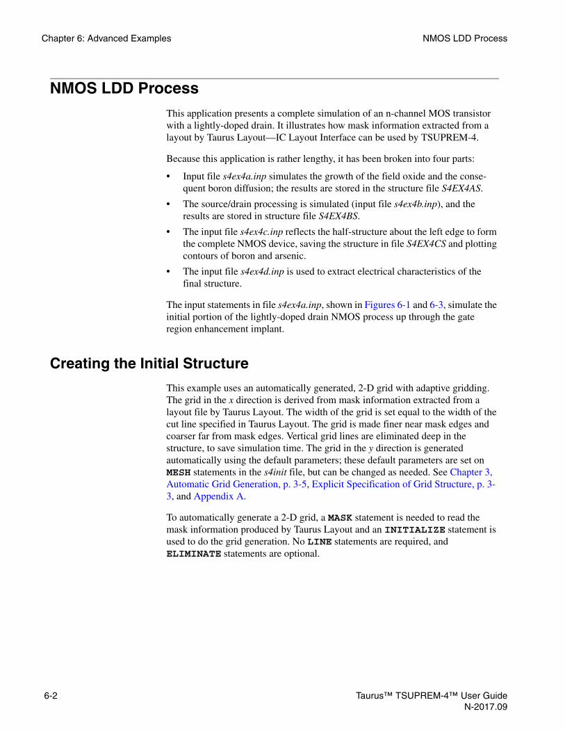
Chapter 6: Advanced Examples NMOS LDD Process

NMOS LDD ProcessThis application presents a complete simulation of an n-channel MOS transistor with a lightly-doped drain. It illustrates how mask information extracted from a layout by Taurus Layout—IC Layout Interface can be used by TSUPREM-4.

Because this application is rather lengthy, it has been broken into four parts:

• Input file s4ex4a.inp simulates the growth of the field oxide and the conse-quent boron diffusion; the results are stored in the structure file S4EX4AS.

• The source/drain processing is simulated (input file s4ex4b.inp), and the results are stored in structure file S4EX4BS.

• The input file s4ex4c.inp reflects the half-structure about the left edge to form the complete NMOS device, saving the structure in file S4EX4CS and plotting contours of boron and arsenic.

• The input file s4ex4d.inp is used to extract electrical characteristics of the final structure.

The input statements in file s4ex4a.inp, shown in Figures 6-1 and 6-3, simulate the initial portion of the lightly-doped drain NMOS process up through the gate region enhancement implant.

Creating the Initial Structure

This example uses an automatically generated, 2-D grid with adaptive gridding. The grid in the x direction is derived from mask information extracted from a layout file by Taurus Layout. The width of the grid is set equal to the width of the cut line specified in Taurus Layout. The grid is made finer near mask edges and coarser far from mask edges. Vertical grid lines are eliminated deep in the structure, to save simulation time. The grid in the y direction is generated automatically using the default parameters; these default parameters are set on MESH statements in the s4init file, but can be changed as needed. See Chapter 3, Automatic Grid Generation, p. 3-5, Explicit Specification of Grid Structure, p. 3-3, and Appendix A.

To automatically generate a 2-D grid, a MASK statement is needed to read the mask information produced by Taurus Layout and an INITIALIZE statement is used to do the grid generation. No LINE statements are required, and ELIMINATE statements are optional.

6-2 Taurus™ TSUPREM-4™ User GuideN-2017.09

NMOS LDD Process Chapter 6: Advanced Examples

Setting the GridDensity

To save execution time, the recommended procedure when developing a new TSUPREM-4 simulation is to start with a very coarse grid. After an input file has been entered and is running correctly (no syntax errors, all etches in the correct places, and so on), a finer grid is used for the bulk of the simulation work. Lastly, an even finer grid is used to get final answers or to verify that additional grid points (with the associated increased execution time) do not significantly improve the accuracy of the answers.

The GRID.FAC parameter on the MESH statement makes it easy to adjust the grid density during the various stages of a simulation project. In this example, GRID.FAC has been set to 1.5, so that all grid spacings are 1.5 times their specified value. This gives a rather coarse grid for efficient simulations.

$ TSUPREM4 NMOS transistor simulation$ Part a: Through field oxidation

$ Define the gridMESH GRID.FAC=1.5$METHOD ERR.FAC=2.0

$ Read the mask definition fileMASK IN.FILE=s4ex4m.tl1 PRINT GRID="Field,Poly"

$ Initialize the structureINITIALIZE <100> BORON=5E15

$ Initial oxidationDIFFUSION TIME=30 TEMP=1000 DRY HCL=5

$ Nitride deposition and field region maskDEPOSIT NITRIDE THICKNESS=0.07 SPACES=4DEPOSIT PHOTORESIST POSITIVE THICKNESS=1EXPOSE MASK=FieldDEVELOPETCH NITRIDE TRAPETCH OXIDE TRAP UNDERCUT=0.1ETCH SILICON TRAP THICKNES=0.25 UNDERCUT=0.1

$ Boron field implantIMPLANT BORON DOSE=5E12 ENERGY=50 TILT=7 ROTATION=30ETCH PHOTORESIST ALL

$ Field oxidationMETHOD PD.TRANS COMPRESSDIFFUSION TIME=20 TEMP=800 T.FINAL=1000DIFFUSION TIME=180 TEMP=1000 WETO2 DIFFUSION TIME=20 TEMP=1000 T.FINAL=800ETCH NITRIDE ALL

$ Unmasked enhancement implantIMPLANT BORON DOSE=1E12 ENERGY=40 TILT=7 ROTATION=30

$ Save structureSAVEFILE OUT.FILE=S4EX4AS

Figure 6-1 First part of input file s4ex4a.inp: Setting up the grid for simulating an NMOS process

Taurus™ TSUPREM-4™ User Guide 6-3N-2017.09

Chapter 6: Advanced Examples NMOS LDD Process

When the results are satisfactory with this grid, GRID.FAC can be decreased to 1.0 or 0.5 to check the results.

AdaptiveGridding

The ERR.FAC parameter on the METHOD statement is used in a similar way to control the accuracy criteria used for adaptive gridding. A value of 2.0 could be used to reduce the accuracy for a faster simulation, but for this example the default value of 1.0 is satisfactory. When the simulation is running correctly, this can be reduced to 0.7 or 0.5 to check the results.

MaskingInformation

The MASK statement reads mask descriptions from the file s4ex4m.tl1. This file, produced by Taurus Layout, describes the mask levels present over a cross-section of the device layout. The PRINT parameter specifies that the mask information should be printed after it is read. The result is shown in Figure 6-2. Four mask levels, named Field, Poly, Contact, and Metal are defined. These names are used to refer to the masks as they are needed later in the processes. The GRID parameter specifies that only the Field and Poly layers in the mask file are considered when calculating the horizontal grid spacing; the Contact and Metal are ignored.

Note:There are no references to mask coordinates in the TSUPREM-4 input file. The mask file contains all the layout information required by the simulation. The same input file can be used to simulate other structures simply by specifying a different mask file.

Field Isolation Simulation

1. The first step is to grow a pad oxide. The default VERTICAL model is suffi-cient for this planar oxidation step; the PD.FERMI model for defects (the default) is acceptable because there is no significant doping in the structure yet.

Figure 6-2 Listing of mask information read from file s4ex4m.tl1

$ Read the mask definition fileMASK IN.FILE=s4ex4m.tl1 PRINT

Comments from mask data file ”s4ex4m.tl1”:/ Mask definition file s4ex4m.tl1, for use with s4ex4[abc].(End of comments from mask data file)

The following masks are currently defined (locations in microns): Name: Field min X: 0.0000 max X: 5.0000 opaque between 0.0000 and 3.9000 Name: Poly min X: 0.0000 max X: 5.0000 opaque between 0.0000 and 0.6500 Name: Contact min X: 0.0000 max X: 5.0000 opaque between 0.0000 and 1.9500 opaque between 3.2500 and 5.0000 Name: Metal min X: 0.0000 max X: 5.0000 opaque between 1.3000 and 5.0000

6-4 Taurus™ TSUPREM-4™ User GuideN-2017.09

NMOS LDD Process Chapter 6: Advanced Examples

2. The next step is to define the active and field isolation regions of the structure. A typical photolithography sequence is used:

a. Deposit a layer to be patterned (nitride, in this case).

b. Deposit a a layer of photoresist (positive resist, in this example).

c. Expose the resist, using the appropriate mask (the Field mask).

d. Use the DEVELOP statement to remove the exposed photoresist.

e. Etch the underlying layers, using the TRAP etch model. The remaining photoresist serves as a mask for the etch. In this case, the nitride is etched first, then the oxide, then the silicon. The oxide and silicon etches specify undercutting of the mask layer by 0.1 and 0.25 microns, respectively.

f. In this example, the photoresist is also used to mask the boron field implant.

g. Remove the remaining photoresist.

Note:You must remove the remaining photoresist at the end of the photolithography sequence.

3. The next step is the field oxidation. The PD.TRANS model is used, resulting in the modeling of interstitials and vacancies, and hence oxidation-enhanced diffusion; the COMPRESS oxidation model is also selected at this point, because all further oxidations will be nonplanar. (If the details of the bird’s beak shape were important, the VISCOEL model with stress dependence could be selected at this point). The field oxidation is done in three steps:

a. For the first 20 minutes, the temperature is ramped up from 800°C to 1000°C at the rate of 10°C/minute in an inert ambient.

b. The second step is a wet oxidation for 180 minutes at a constant tempera-ture of 1000°C.

c. Finally, the temperature is ramped down from 1000°C to 800°C at the rate of 10°C/minute in an inert ambient.

4. The final process steps specified in the first input file are the removal of the nitride oxidation mask and the implantation of boron for adjusting the n-chan-nel threshold voltage.

The structure to this point is saved in the structure file S4EX4AS for use in continued simulation of the source and drain regions.

Displaying thePlot

Figure 6-3 shows the input statements for displaying the results thus far. The first PLOT.2D statement plots the grid at this point (Figure 6-4). As planned, the grid is fairly coarse; some refinement by adaptive gridding is evident near the surface and around the field oxide. The structure at this point is shown in Figure 6-5. Contour lines of boron concentration are plotted starting at a concentration of 1015 and extending up to a concentration of 1020 atoms/cm3 in half-decade steps.

Taurus™ TSUPREM-4™ User Guide 6-5N-2017.09

Chapter 6: Advanced Examples NMOS LDD Process

$ Plot the initial NMOS structureSELECT Z=LOG10(BORON) TITLE="LDD Process - NMOS Isolation Region"PLOT.2D SCALE GRID C.GRID=2 Y.MAX=2.0PLOT.2D SCALE Y.MAX=2.0

$ Color fill the regionsCOLOR SILICON COLOR=7COLOR OXIDE COLOR=5

$ Plot contours of boronFOREACH X (15 TO 20 STEP 0.5) CONTOUR VALUE=X LINE=5 COLOR=2END

$ Replot boundariesPLOT.2D ^AX ^CL

$ Print doping information under field oxideSELECT Z=DOPINGPRINT.1D X.VALUE=4.5 X.MAX=3

Figure 6-3 Second part of input file s4ex4a.inp, for simulating an NMOS process

Figure 6-4 Grid after formation of isolation region, plotted by s4ex4a.inp

0.00 2.00 4.00Distance (µm)

Dis

tanc

e (µ

m)

2.00

0.00

LDD Process − NMOS Isolation Region

6-6 Taurus™ TSUPREM-4™ User GuideN-2017.09

NMOS LDD Process Chapter 6: Advanced Examples

Active Region Simulation

The input statements in the file s4ex4b.inp complete the processing of the NMOS transistor. The listing of this input file is presented in Figures 6-6 and 6-8. The starting structure for this stage of the simulation is read from the file S4EX4AS generated by the simulation input file s4ex4a.inp. The grid spacing and error control factors are not saved in the structure file, so they must be reset to their desired values with the MESH and METHOD statements, respectively. Similarly, the mask information from Taurus Layout must be reread with the MASK statement.

The first process steps in this input file define and oxidize a polysilicon gate. The Poly mask is used in a typical photolithography sequence (that is, DEPOSITION, EXPOSE, DEVELOP, and ETCH). The COMPRESS model is used to simulate the oxidation of the polysilicon gate and the PD.TRANS model is used for diffusion. These models are not explicitly specified in input file s4ex4b.inp; rather, they are set in s4ex4a.inp, saved (automatically) in the structure file S4EX4AS, and then read in by the INITIALIZE statement in s4ex4b.inp.

ModelingPolysilicon

The statement MATERIAL MAT=POLY ^POLYCRYS disables the advanced models for grain growth and impurity diffusion in polysilicon (to reduce the computation time). For studying the details of impurity diffusion and activation in the gate, this statement would be omitted. Also, a finer grid would be used in the poly, either by specifying more grid spaces in the DEPOSITION statement or by reducing the relative error for adaptive gridding in polysilicon (that is, by specifying a smaller value for REL.ADAP for impurities in poly).

Figure 6-5 Structure with contours of boron concentration, after formation of isolation region, as plotted by file s4ex4a.inp

0.00 2.00 4.00Distance (µm)

Dis

tanc

e (µ

m)

2.00

0.00

LDD Process − NMOS Isolation Region

Taurus™ TSUPREM-4™ User Guide 6-7N-2017.09

Chapter 6: Advanced Examples NMOS LDD Process

LDD Implant Next, the lightly doped source/drain region extension is implanted. Because the implantation is through an oxide, IMPL.TAB=arsenic is used instead of the default dual-Pearson implant moments (the dual.ars tables) with channelling tails. The mesh nodes needed to resolve the implanted profile are added automatically through adaptive gridding.

$ TSUPREM4 NMOS transistor simulation$ Part b: Through source/drain metallization

$ Set grid spacing and accuracy parametersMESH GRID.FAC=1.5$METHOD ERR.FAC=2.0

$ Read structure from initial simulationINITIAL IN.FILE=S4EX4AS

$ Read the mask definition fileMASK IN.FILE=s4ex4m.tl1

$ Define polysilicon gateMATERIAL MAT=POLY ^POLYCRYSDEPOSIT POLYSILICON THICK=0.4 SPACES=2DEPOSIT PHOTORESIST THICK=1.0EXPOSE MASK=PolyDEVELOPETCH POLYSILICON TRAP THICK=0.7 ANGLE=79ETCH PHOTORESIST ALL

$ Oxidize the polysilicon gateDIFFUSION TIME=30 TEMP=1000 DRYO2 $ LDD implant at a 7-degree tiltIMPLANT ARSENIC DOSE=5E13 ENERGY=50 TILT=7.0 ROTATION=30 IMPL.TAB=ARSENIC

$ Plot structureSELECT Z=LOG10(BORON) TITLE="LDD Process - After LDD Implant"PLOT.2D SCALE Y.MAX=2.0

$ Add color fillCOLOR SILICON COLOR=7COLOR OXIDE COLOR=5COLOR POLY COLOR=3

$ Plot contoursFOREACH X (15 TO 18 STEP 0.5) CONTOUR VALUE=X LINE=5 COLOR=2ENDSELECT Z=LOG10(ARSENIC)FOREACH X (16 TO 20)

CONTOUR VALUE=X LINE=2 COLOR=4END

$ Replot boundariesPLOT.2D ^AX ^CL

Figure 6-6 First part of input file s4ex4b.inp, showing polysilicon gate formation

6-8 Taurus™ TSUPREM-4™ User GuideN-2017.09

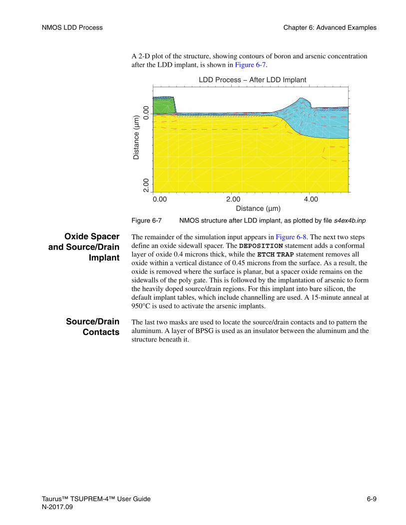
NMOS LDD Process Chapter 6: Advanced Examples

A 2-D plot of the structure, showing contours of boron and arsenic concentration after the LDD implant, is shown in Figure 6-7.

Oxide Spacerand Source/Drain

Implant

The remainder of the simulation input appears in Figure 6-8. The next two steps define an oxide sidewall spacer. The DEPOSITION statement adds a conformal layer of oxide 0.4 microns thick, while the ETCH TRAP statement removes all oxide within a vertical distance of 0.45 microns from the surface. As a result, the oxide is removed where the surface is planar, but a spacer oxide remains on the sidewalls of the poly gate. This is followed by the implantation of arsenic to form the heavily doped source/drain regions. For this implant into bare silicon, the default implant tables, which include channelling are used. A 15-minute anneal at 950°C is used to activate the arsenic implants.

Source/DrainContacts

The last two masks are used to locate the source/drain contacts and to pattern the aluminum. A layer of BPSG is used as an insulator between the aluminum and the structure beneath it.

Figure 6-7 NMOS structure after LDD implant, as plotted by file s4ex4b.inp

0.00 2.00 4.00Distance (µm)

Dis

tanc

e (µ

m)

2.00

0.00

LDD Process − After LDD Implant

Taurus™ TSUPREM-4™ User Guide 6-9N-2017.09

Chapter 6: Advanced Examples NMOS LDD Process

$ Define the oxide sidewall spacerDEPOSIT OXIDE THICK=0.4ETCH OXIDE THICK=0.45 TRAP

$ Heavy S/D implant at a 7-degree tiltIMPLANT DOSE=1E15 ENERGY=200 ARSENIC TILT=7.0 ROTATION=30

$ Anneal to activate the arsenicDIFFUSION TIME=15 TEMP=950 $ Deposit BPSG and cut source/drain contact holesDEPOSIT OXIDE THICKNES=0.7DEPOSIT PHOTORESIST POSITIVE THICKNESS=1.0EXPOSE MASK=ContactDEVELOPETCH OXIDE THICKNESS=1.0 TRAP ANGLE=75ETCH PHOTORESIST ALL $ Define the metallizationDEPOSIT ALUMINUM THICKNESS=1.0DEPOSIT PHOTORESIST POSITIVE THICKNESS=1.0EXPOSE MASK=MetalDEVELOPETCH ALUMINUM TRAP THICKNESS=1.5 ANGLE=75ETCH PHOTORESIST ALL

$ Save the final structureSAVEFILE OUT.FILE=S4EX4BS $ Plot the half NMOS structureSELECT Z=LOG10(BORON) TITLE="LDD Process - Half of NMOS Structure"PLOT.2D SCALE Y.MAX=2.0 GRID C.GRID=2PLOT.2D SCALE Y.MAX=2.0

$ Color fillCOLOR SILICON COLOR=7COLOR OXIDE COLOR=5COLOR POLY COLOR=3COLOR ALUM COLOR=2

$ Plot contoursFOREACH X (15 TO 18 STEP 0.5) CONTOUR VALUE=X LINE=5 COLOR=2END SELECT Z=LOG10(ARSENIC)FOREACH X (15 TO 20) CONTOUR VALUE=X LINE=2 COLOR=4END

$ Replot boundariesPLOT.2D ^AX ^CL

$ Print doping through drainSELECT Z=DOPINGPRINT.1D LAYERS X.VALUE=2

Figure 6-8 Second part of input file s4ex4b.inp, showing source/drain processing and metallization

6-10 Taurus™ TSUPREM-4™ User GuideN-2017.09

NMOS LDD Process Chapter 6: Advanced Examples

Plots The final grid is plotted in Figure 6-9. Adaptive gridding has produced a fine grid where it is needed: in the source/drain region and particularly in the lightly doped extension. The 2-D contour plot of the boron and arsenic concentrations (Figure 6-10) shows that the shallow extension of the source/drain region is well defined. The results of the drain region simulation are saved with the SAVEFILE statement in the structure file S4EX4BS. This file is used as the basis for forming the complete NMOS device.

Figure 6-9 Final grid for LDD NMOS example, produced by input files s4ex4a.inp and s4ex4b.inp

0.00 2.00 4.00Distance (µm)

Dis

tanc

e (µ

m)

2.00

0.00

LDD Process − Half of NMOS Structure

-2.0

0

Taurus™ TSUPREM-4™ User Guide 6-11N-2017.09

Chapter 6: Advanced Examples NMOS LDD Process

Formation of the Complete NMOS Transistor

The complete NMOS transistor is formed by reading in the right half of the structure from the previous simulation and reflecting it about its left edge. The final structure is then plotted, and the various material regions are shaded and labeled. Contours of boron (long dashes) and arsenic (medium dashes) are plotted. The completed structure is saved in file S4EX4CS. The input statements for doing this are shown in Figure 6-11; the resulting plot is shown in Figure 6-12.

Figure 6-10 Final NMOS structure, as plotted by file s4ex4b.inp

0.00 2.00 4.00Distance (µm)

Dis

tanc

e (µ

m)

2.00

0.00

LDD Process − Half of NMOS Structure

-2.0

0

6-12 Taurus™ TSUPREM-4™ User GuideN-2017.09

NMOS LDD Process Chapter 6: Advanced Examples

Figure 6-11 Input file s4ex4c.inp, for plotting the final LDD NMOS structure

$ TSUPREM4 NMOS transistor simulation$ Part c: Formation of complete structure

$ Read right half of structure INITIAL IN.FILE=S4EX4BS

$ Reflect about the left edge to form the complete structureSTRUCTURE REFLECT LEFT $ Plot the complete NMOS structureSELECT Z=LOG10(BORON) TITLE=”Example 4 - Complete NMOS Structure”PLOT.2D SCALE Y.MAX=2.0 Y.MIN=-3.0

$ Color fillCOLOR SILICON COLOR=7LABEL X=-4.1 Y=-2.5 LABEL=”Silicon” SIZE=.3 C.RECT=7 W.RECT=.4 H.R=.4COLOR POLYSILI COLOR=3LABEL X=-1.8 Y=-2.5 LABEL=”Polysilicon” SIZE=.3 C.RECT=3 W.RECT=.4 H.R=.4COLOR OXIDE COLOR=5LABEL X=1.2 Y=-2.5 LABEL=”Oxide” SIZE=.3 C.RECT=5 W.RECT=.4 H.R=.4COLOR ALUMINUM COLOR=2LABEL X=3.2 Y=-2.5 LABEL=”Aluminum” SIZE=.3 C.RECT=2 W.RECT=.4 H.R=.4

$ Plot contoursFOREACH X (15 16 17 18) CONTOUR VAL=X LINE=5 COLOR=2END SELECT Z=LOG10(ARSENIC)FOREACH X (15 16 17 18 19 20) CONTOUR VAL=X LINE=3 COLOR=4END

$ Replot boundariesPLOT.2D ^AX ^CL SAVEFILE OUT.FILE=S4EX4CS

Figure 6-12 Complete NMOS structure, plotted by input file s4ex4c.inp

-4.00 -2.00 2.00Distance (µm)

Dis

tanc

e (µ

m)

2.00

-2.0

0

0.00 4.00

Silicon Polysilicon Oxide Aluminum

Taurus™ TSUPREM-4™ User Guide 6-13N-2017.09

Chapter 6: Advanced Examples NMOS LDD Process

Electrical Extraction

This example shows the extraction of the following electrical information:

• Threshold voltage

• Gate capacitance

• Source/Drain junction capacitance

The statements for performing the electrical extraction are in the input file s4ex4d.inp.

Electrical extraction is specified by the ELECTRICAL statement. Results are calculated along a vertical slice through the device specified by the value of the X parameter. The type of extraction is specified by the THRESHOLD, MOSCAP, JCAP, and RESISTAN parameters.

ThresholdVoltage

The THRESHOLD parameter is used to extract the threshold voltage. The NMOS parameter specifies that the type of MOS transistor is NMOS. The position X is located at the center of the gate. The gate voltage V is stepped from 0 to 2 volts in 0.1-volt increments. The other regions (that is, the source, drain, and bulk) are grounded. The surface state density QSS defaults to 1x1010/cm2.

Because TSUPREM-4 solves the 1-D Poisson equation, the extracted quantity is not drain current, but sheet conductance of the channel. However, the drain current can be approximately calculated from the sheet conductance, assuming that the channel is long and wide so that small-geometry effects can be neglected. This example supposes that NMOS with channel length of 1.2 microns and width of 25 microns is measured and that the drain is biased to 0.1 volt to minimize lowering of the energy barrier in the channel region. The scaling factor is the drain voltage multiplied by W/L. ASSIGN statements are used to set the values of length, width, and drain voltage and to calculate the scale factor.

The shift in the threshold voltage due to the body effect is examined by changing the back bias. The value of the body-effect parameter is approximately equal to the difference between the threshold voltages at 0and 2.5-volts back bias. This example shows approximately 0.9-volt threshold voltage shift and approximately 1.0-V1/2 body effect.

6-14 Taurus™ TSUPREM-4™ User GuideN-2017.09

NMOS LDD Process Chapter 6: Advanced Examples

The input statements for extracting and plotting the threshold characteristics are shown in Figure 6-13; the results are shown in Figure 6-16.

MOSCapacitance

Many process monitoring parameters—the grown oxide thickness, the surface state density, the flat band voltage, and the mobile charge in oxide, for example—are extracted from MOS C-V measurements during manufacturing. While transient device simulations are required for rigorous analysis of gate capacitance as a function of frequency, TSUPREM-4 can give reasonably accurate simulations of gate capacitance if a sufficiently high frequency (above 100 kHz) is assumed.

The parameter MOSCAP specifies that the MOS capacitance is extracted. Depending on the input frequency compared with the lifetime of carriers in the channel, there are three types of C-V plot.

1. In most cases, the input signal is composed of a slow bias signal and fast AC signal. This is the normal C-V plot, which is specified by HIGH (the default) in TSUPREM-4.

2. The second assumes a slow bias signal and a low-frequency AC input signal; that is specified by the LOW parameter.

3. Finally, if a fast bias sweep is performed with a high-frequency AC signal so that the inversion charge does not have time to accumulate, the depletion region expands deeper into the substrate. The DEEP parameter specifies this.

In this example, gate bias V is increased from -5 to 5 volts in 0.2-volt steps. The capacitance is calculated from dQ/dV. The perturbed AC bias, dV is calculated

$ TSUPREM-4 - Electrical Extraction

$ Read structure from Example 4 INITIAL IN.FILE=S4EX4CS

$ Part A: Threshold voltage$ Extract the gate bias vs. the sheet conductance in channel region$ -- VBS=0V ELECTRIC X=0.0 THRESHOLD NMOS V="0 2 0.1" OUT.FILE=S4EX4DS1

$ -- VBS=-2.5V ELECTRIC X=0.0 THRESHOLD NMOS V="0 3 0.05" VB=-2.5 OUT.FILE=S4EX4DS2

$ Plot the Vgs vs Ids$ -- Define the scale to convert the sheet conductance to the currentASSIGN NAME=Lch N.VAL=1.2ASSIGN NAME=Wch N.VAL=25.0ASSIGN NAME=Vds N.VAL=0.1ASSIGN NAME=Scale N.VAL=(@Vds*@Wch/@Lch)$ -- PlotSELECT TITLE="Vgs vs. Ids"VIEWPORT X.MAX=0.5PLOT.1D IN.FILE=S4EX4DS1 Y.SCALE=@Scale + Y.LABEL="I(Drain) (Amps)" X.LABEL="V(Gate) (Volts)" + TOP=1E-4 BOT=0 RIGHT=3.5 COLOR=2PLOT.1D IN.FILE=S4EX4DS2 Y.SCALE=@Scale ̂ CL ̂ AX COLOR=3 LINE=2LABEL LABEL="Vbs=0" X=1.9 Y=9E-5 RIGHTLABEL LABEL="Vbs=-2.5" X=3.35 Y=7.6E-5 RIGHT

Figure 6-13 First part of input file s4ex4d.inp, showing the threshold voltage extraction

Taurus™ TSUPREM-4™ User Guide 6-15N-2017.09

Chapter 6: Advanced Examples NMOS LDD Process

from the DC increment multiplied by a constant E.RVCAP, which is defined as the ratio of AC amplitude to DC increment in the METHOD statement (default value of 0.2 or 20%). The perturbed AC bias in this example is 0.04 V(= 0.2 V x 0.2). For example, the capacitance at 1 V is extracted from the charge variation between 0.96 V and 1.04 V. The input statements for extracting the MOS capacitance are shown in Figure 6-14; the results are shown in Figure 6-16.

Source/DrainJunction

Capacitance

The junction capacitance between source (or drain) and bulk is one of important parameters to determine the delay characteristics of the MOS transistor. This capacitance is composed of two kinds of capacitance: areal and peripheral capacitance. In device characterization, these two components are separated and characterized by universal parameters independent of the shape of device. Usually, the areal capacitance is dominant. TSUPREM-4 extracts the areal junction capacitance (in F/cm2) when the JCAP parameter is specified.

The JUNCTION parameter selects the junction to be analyzed. Junctions are numbered from the bottom of the structure to the top, with the deepest junction being junction number one. For example, if X specifies the emitter region of a bipolar transistor, there might be three junctions: E-B (emitter-base, junction number 3), B-C (base-collector, junction number 2), and C-S (collector-substrate, junction number 1). In this example, there is only one junction, identified as number 1.

The input bias V must be all positive or all negative including zero bias. TSUPREM-4 chooses the biased region by considering the polarity of the input voltage so that the junction is reverse biased. All regions except for the biased region are grounded. The perturbed AC bias is applied using the same method as in the MOS capacitance.

$ Part B: C-V plot for MOS capacitance$ Extract the capacitance

$ -- High FrequencyELECTRIC X=0.0 MOSCAP NMOS V=”-5 5 0.2” OUT.F=S4EX4DS3$ -- Low FrequencyELECTRIC X=0.0 MOSCAP NMOS V=”-5 5 0.2” LOW OUT.F=S4EX4DS4$ -- Deep depletion ELECTRIC X=0.0 MOSCAP NMOS V=”-5 5 0.2” DEEP

$ Plot the C-V curveSELECT TITLE=”MOS C-V”VIEWPORT X.MIN=0.5 Y.MIN=0.51PLOT.1D ELECTRIC COLOR=2 TOP=1E-7 BOT=0 LEFT=-6 RIGHT=6 + X.OFF=1.5 ^CLPLOT.1D IN.FILE=S4EX4DS3 ^CL ^AX COLOR=3 LINE=2PLOT.1D IN.FILE=S4EX4DS4 ^CL ^AX COLOR=4 LINE=3LABEL LABEL=”Low” X=3 Y=8.3E-8LABEL LABEL=”High” X=3 Y=3.7E-8LABEL LABEL=”Deep” X=3 Y=0.7E-8

Figure 6-14 Second part of input file s4ex4d.inp, showing the MOS capacitance extraction

6-16 Taurus™ TSUPREM-4™ User GuideN-2017.09

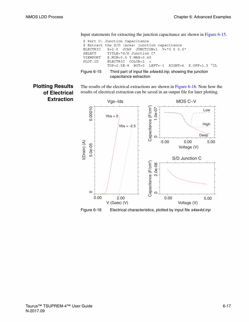
NMOS LDD Process Chapter 6: Advanced Examples

Input statements for extracting the junction capacitance are shown in Figure 6-15.

Plotting Resultsof Electrical

Extraction

The results of the electrical extractions are shown in Figure 6-16. Note how the results of electrical extraction can be saved in an output file for later plotting.

$ Part C: Junction Capacitance$ Extract the S/D (area) junction capacitanceELECTRIC X=2.0 JCAP JUNCTION=1 V="0 5 0.5"SELECT TITLE="S/D Junction C"VIEWPORT X.MIN=0.5 Y.MAX=0.49PLOT.1D ELECTRIC COLOR=2 + TOP=2.5E-8 BOT=0 LEFT=-1 RIGHT=6 X.OFF=1.5 ^CL

Figure 6-15 Third part of input file s4ex4d.inp, showing the junction capacitance extraction

Figure 6-16 Electrical characteristics, plotted by input file s4ex4d.inp

Vgs−Ids MOS C−V

S/D Junction C

-5.00 0.00 5.00

0.00 5.00

Voltage (V)

Voltage (V)

Cap

acita

nce

(F/c

m2 )

02.

0e-0

8

Cap

acita

nce

(F/c

m2 )

01.

0e-0

7

0

I(D

rain

) (A

)

5.0e

-05

0.00

010

0.00 2.00V (Gate) (V)

Vbs = 0

Vbs = -2.5

Low

High

Deep

Taurus™ TSUPREM-4™ User Guide 6-17N-2017.09

Chapter 6: Advanced Examples Trench Implant Simulation

Trench Implant SimulationThis example shows two methods for performing a tilted ion implantation into a trench. First, TSUPREM-4’s analytical model is used to implant ions at a 15° tilt. Next, TSUPREM-4’s Monte Carlo (MC) method is used to perform the same implantation. The results of the two methods are compared and contrasted.

Figure 6-17 First part of input file s4ex5.inp, showing grid setup

$ TSUPREM-4 Example 5 - Implant Trench Application$$ Simulate ion implantation into a trench using the analytical approach$ followed by the Monte Carlo approach.

$ Place the finest grid around the trenchLINE X LOCATION=0.0 SPACING=1.0LINE X LOCATION=0.25 SPACING=0.01LINE X LOCATION=0.32 SPACING=0.01LINE X LOCATION=0.5 SPACING=0.2

LINE Y LOCATION=0.0 SPACING=0.01LINE Y LOCATION=0.05 SPACING=0.01LINE Y LOCATION=0.92 SPACING=0.04LINE Y LOCATION=1.0 SPACING=0.01LINE Y LOCATION=1.05 SPACING=0.01LINE Y LOCATION=1.2 SPACING=1.0

ELIMINATE ROWS X.MAX=0.2 Y.MIN=0.15 Y.MAX=1.0ELIMINATE ROWS X.MAX=0.25 Y.MIN=1.0 Y.MAX=1.1ELIMINATE COLUMNS X.MIN=0.23 X.MAX=0.35 Y.MIN=1.1ELIMINATE COLUMNS X.MIN=0.25 X.MAX=0.34 Y.MIN=1.1

$ Initialize the structureINITIALIZE BORON=2E15

$ Etch the left half of the trenchETCH START X=0.3 Y=0.0ETCH CONTINUE X=0.3 Y=0.5ETCH CONTINUE X=0.32 Y=0.9ETCH CONTINUE X=0.34 Y=0.95ETCH CONTINUE X=0.4 Y=1.0ETCH CONTINUE X=2.0 Y=1.0ETCH DONE X=2.0 Y=0.0

$ Form the complete trench structureSTRUCTURE REFLECT

$ Save the structureSAVEFILE OUT.FILE=S4EX5S

$ Plot the gridSELECT TITLE=”Grid for Trench Application”PLOT.2D SCALE GRID C.GRID=2

6-18 Taurus™ TSUPREM-4™ User GuideN-2017.09

Trench Implant Simulation Chapter 6: Advanced Examples

Structure Generation

The input statements for this simulation are shown in Figures 6-17, 6-19, and6-23. The initial mesh setup uses the symmetry of the trench structure, as suggested by SEM photographs of trenches generated by reactive ion etching. The initial grid, established by the LINE and ELIMINATE statements, is for the left half of the trench only. Particular attention has been given to producing a fine grid where the side and bottom walls of the trench are formed to resolve the implanted profiles. The ELIMINATE statements reduce the number of grid points in areas where the implant is not expected to penetrate. The sequence of ETCH statements specifies geometrically the shape of the left half of the trench structure. The resulting half-structure is reflected to generate the full structure, using the REFLECT parameter on the STRUCTURE statement. The full structure is saved with the SAVEFILE statement.

The grid for the full structure is then plotted (Figure 6-18). Note that a fine mesh has been placed around the trench, without wasting nodes in the lower corners.

Analytic Implant

The boron implant is now performed at an energy of 5 keV. In the absence of the MONTECAR parameter, TSUPREM-4 uses the analytic method. The TILT parameter is used to specify that the angle of the incident ion beam is 15° counterclockwise from the vertical (that is, the beam enters from the left). The implant is followed by a short diffusion to activate the boron and anneal implant damage.

Figure 6-18 Grid for trench implant example

0.50 1.00Distance (µm)

Dis

tanc

e (µ

m)

1.00

0.00

0.00

0.50

Taurus™ TSUPREM-4™ User Guide 6-19N-2017.09

Chapter 6: Advanced Examples Trench Implant Simulation

Figure 6-19 Second part of input file s4ex5.inp, showing tilted implantation using analytic implant model

$ Analytic implant at a 15-degree tilt to dope the trench sidewallsIMPLANT BORON ENERGY=5 DOSE=1E14 TILT=15

$ A short annealDIFFUSION TIME=5 TEMP=900

$ 2D contour plot of boron contoursSELECT Z=LOG10(BORON) TITLE=”Contours of Boron (Analytic)”PLOT.2D SCALE X.MAX=1.5FOREACH X (16 TO 21 STEP 1)

COLOR MIN.V=X MAX.V=( X + 1) COLOR=( X - 2)ENDPLOT.2D ^AXES ^CLEARLABEL X=1.05 Y=0.25 LABEL=”Log10(Boron)” SIZE=0.3LABEL X=1.15 Y=0.33 LABEL=”16-17” SIZE=0.3 C.RECT=14 W.R=0.4 H.R=0.4LABEL X=1.15 Y=0.41 LABEL=”17-18” SIZE=0.3 C.RECT=15 W.R=0.4 H.R=0.4LABEL X=1.15 Y=0.49 LABEL=”18-19” SIZE=0.3 C.RECT=16 W.R=0.4 H.R=0.4LABEL X=1.15 Y=0.57 LABEL=”19-20” SIZE=0.3 C.RECT=17 W.R=0.4 H.R=0.4LABEL LABEL=”Tilt angle=15 degrees” X=0.02 Y=1.18

$ 1D plots of boron

$ Vertical profilesSELECT Z=LOG10(BORON) TITLE=”Vertical Profiles (Analytic)”PLOT.1D X.VALUE=0.1 TOP=21 BOTTOM=15 RIGHT=1.2 COLOR=2LABEL X=0.06 Y=19 LABEL=”Surface”LABEL X=0.06 Y=18.8 LABEL=”(x=0.1)”

PLOT.1D X.VALUE=0.5 ^AXES ^CLEAR COLOR=2LABEL X=1.05 Y=18.5 LABEL=”Trench”LABEL X=1.05 Y=18.3 LABEL=”(x=0.5)”

$ Horizontal profilesDEPOSIT OXIDE THICK=0.002SELECT Z=LOG10(BORON) TITLE=”Sidewall Profiles at y=0.2 (Analytic)”PLOT.1D Y.VALUE=0.2 LEFT=0.1 RIGHT=0.9 BOTTOM=15 TOP=21 COLOR=2

$ Print profile through bottom of trenchPRINT.1D X.VALUE=0.5

6-20 Taurus™ TSUPREM-4™ User GuideN-2017.09

Trench Implant Simulation Chapter 6: Advanced Examples

Plotting the Results of the Analytic Method

Figure 6-20 shows shaded contours of boron concentration produced by the COLOR statement and associated SELECT, PLOT.2D, FOREACH, END, and LABEL statements. Observe that dopant is present only on the right side of the trench where the ions are directly incident. This is because the analytic method does not account for reflected ions. The profile at the bottom right corner of the trench (where boron is directly incident) is approximately the same as that on the surface of the silicon.

Figure 6-21 shows 1-D boron profiles vertically through the middle of the trench bottom and at the surface of the silicon. The peak boron concentration is much greater at the silicon surface than at the bottom of the trench due to shadowing of the bottom by the sidewalls.

Figure 6-22 shows the boron concentration on the left and right sides of the trench at a depth of y=0.2 microns. The flat profile on the left hand side, at a value nearly that of the background concentration, confirms the lack of reflected ions when the analytic method is used. The corresponding plot for the MC implantation model is very different.

(A thin layer of oxide is deposited to ensure that the structure boundaries are correctly plotted by the PLOT.1D statement. Without the added oxide, the section at y=0.2 would pass through silicon, ambient, and silicon as x varies from 0 to 1.0 microns.

Due to a limitation in the current version of the program, the silicon/ambient and ambient/silicon interfaces are only recognized at the edges of the structure, but not in its interior. By adding the thin layer of oxide, silicon/oxide and oxide/silicon

Figure 6-20 Contours of boron after analytic implant

0.50 1.00 1.50Distance (µm)

Dis

tanc

e (µ

m)

1.00

0.00

0.00

0.50

Log10(Boron)

16−1717−1818−1919−20

Tilt angle=15 degrees

Taurus™ TSUPREM-4™ User Guide 6-21N-2017.09

Chapter 6: Advanced Examples Trench Implant Simulation

boundaries are added. These boundaries are plotted correctly in Figures 6-20 and 6-26).

Figure 6-21 Vertical profiles produced by analytic implant

Figure 6-22 Sidewall profiles produced by analytic implant

0.50 1.00Distance (µm)

Log1

0(B

oron

)

0.00

21

20

19

18

17

16

15

Vertical Profiles (Analytic)

Surface(x=0.1) Trench

(x=0.5)

0.60 0.80Distance (µm)

Log1

0(B

oron

)

0.20

21

20

19

18

17

16

150.40

Sidewall Profiles at y=0.2 (Analytic)

6-22 Taurus™ TSUPREM-4™ User GuideN-2017.09

Trench Implant Simulation Chapter 6: Advanced Examples

MC Implant

The second half of the simulation demonstrates the use of the MC implantation method.

Overview Unlike the analytic approach, the MC algorithm accurately models the effect of reflected ions in a trench structure. The MC calculation follows the trajectories of individual ions through each material present in the structure; ion trajectories through a vacuum, including those reflected off trench sidewalls, are calculated in exactly the same way as through other materials. The velocity of a reflected ion remains constant until it enters a material other than vacuum or leaves the top or bottom of the simulated structure. For ions that leave either side of the simulation space, the appropriate boundary condition (periodic, reflecting, or vacuum) is invoked.

Using the MCModel

The first step in the MC portion of the simulation is to read in the trench structure, just prior to the analytic implant. The boron implant is performed once again, but this time the MONTECAR parameter on the IMPLANT statement directs TSUPREM-4 to use the MC implant model. The ENERGY, DOSE, and TILT parameters are the same as those used during the analytic implant.

In addition to the MONTECAR parameter, two new parameters are now specified:

• N.ION—The N.ION parameter specifies the number of ion trajectories to calculate. The simulation time is directly proportional to the number of ion trajectories calculated. Decreasing this number, however, increases the statis-tical noise in the output of the MC calculation.

• ^CRYSTAL—The specification of ^CRYSTAL on the IMPLANT command disables the crystal model for ion penetration in silicon. This speeds the calcu-lation significantly by eliminating the calculation of channeling and damage effects.

A short post-implant anneal is performed as before to activate the implant. The diffusion also acts to smooth the results of the MC calculation.

Plotting the Results of the MC Method

The three figures output after the MC implant (Figures 6-24 through 6-26) are the counterparts of the three analytic plots (Figures 6-20 through 6-22).

Boron Contours Figure 6-24 shows the contours of boron concentration produced by the MC method. Note that dopant is present in substantial quantities on the left side of the trench (unlike the analytic results). The plot illustrates that dopant is present in greater quantity on the right side of the trench where the ions are directly incident. The boron in the left side of the trench is due entirely to reflection of ions. As before, the profile at the bottom right corner of the trench is approximately the same as that on the surface of the silicon.

Taurus™ TSUPREM-4™ User Guide 6-23N-2017.09

Chapter 6: Advanced Examples Trench Implant Simulation

Vertical Profiles Figure 6-25, shows 1-D boron profiles vertically through the middle of the trench bottom and at the surface of the silicon for the MC implant. The peak boron concentration is approximately a factor of five greater at the silicon surface than at the bottom of the trench due to shadowing of the bottom by the sidewalls. Observe that the difference between the peaks is much less for the MC approach than the analytic method. This is due to the reflected ion calculations included in the MC algorithm. The depth of the implant is less at the bottom of the trench than at the silicon surface, due to the loss of energy when an ion is reflected.

Figure 6-23 Third part of file s4ex5.inp, using the MC implantation model

$ Repeat the implantation using the Monte Carlo method

$ Read in the structureLOADFILE IN.FILE=S4EX5S

$ Monte Carlo implant at a 15-degree tilt to dope the trench sidewallsIMPLANT BORON ENERGY=5 DOSE=1E14 MONTECAR TILT=15 N.ION=10000 ^CRYSTAL

$ A short annealDIFFUSION TIME=5 TEMP=900

$ 2D contour plot of boron contoursSELECT Z=LOG10(BORON) TITLE=”Contours of Boron (Monte Carlo)”PLOT.2D SCALE X.MAX=1.5FOREACH X (16 TO 21 STEP 1)

COLOR MIN.V=X MAX.V=( X + 1) COLOR=( X - 2)ENDPLOT.2D ^AXES ^CLEARLABEL X=1.05 Y=0.25 LABEL=”Log10(Boron)” SIZE=0.3LABEL X=1.15 Y=0.33 LABEL=”16-17” SIZE=0.3 C.RECT=14 W.R=0.4 H.R=0.4LABEL X=1.15 Y=0.41 LABEL=”17-18” SIZE=0.3 C.RECT=15 W.R=0.4 H.R=0.4LABEL X=1.15 Y=0.49 LABEL=”18-19” SIZE=0.3 C.RECT=16 W.R=0.4 H.R=0.4LABEL X=1.15 Y=0.57 LABEL=”19-20” SIZE=0.3 C.RECT=17 W.R=0.4 H.R=0.4LABEL LABEL=”Tilt angle=15 degrees” X=0.02 Y=1.18

$ 1D plots of boron

$ Vertical profilesSELECT Z=LOG10(BORON) TITLE=”Vertical Profiles (Monte Carlo)”PLOT.1D X.VALUE=0.1 TOP=21 BOTTOM=15 RIGHT=1.2 COLOR=2LABEL X=0.06 Y=19 LABEL=”Surface”LABEL X=0.06 Y=18.8 LABEL=”(x=0.1)”

PLOT.1D X.VALUE=0.5 ^AXES ^CLEAR COLOR=2LABEL X=1.05 Y=18.5 LABEL=”Trench”LABEL X=1.05 Y=18.3 LABEL=”(x=0.5)”

$ Horizontal profilesDEPOSIT OXIDE THICK=0.002SELECT Z=LOG10(BORON) TITLE=”Sidewall Profiles at y=0.2 (Monte Carlo)”PLOT.1D Y.VALUE=0.2 LEFT=0.1 RIGHT=0.9 BOTTOM=15 TOP=21 COLOR=2

$ Print profile through bottom of trenchPRINT.1D X.VALUE=0.5

6-24 Taurus™ TSUPREM-4™ User GuideN-2017.09

Trench Implant Simulation Chapter 6: Advanced Examples

Comparing the vertical profiles produced by the analytic and MC models (Figures 6-21 and 6-25, respectively), shows that the boron penetrates more deeply with the analytic model than with the MC approach. This is due to the specification of ^CRYSTAL during the MC implantation. This causes the silicon to be treated as amorphous, which speeds the calculation significantly but prevents calculation of channeling in the crystal structure.

Figure 6-24 Contours of boron after Monte Carlo implant

0.50 1.00 1.50Distance (µm)

Dis

tanc

e (µ

m)

1.00

0.00

0.00

0.50

Log10(Boron)

16−1717−1818−1919−20

Tilt angle=15 degrees

Taurus™ TSUPREM-4™ User Guide 6-25N-2017.09

Chapter 6: Advanced Examples Trench Implant Simulation

In contrast, the analytic method automatically includes the channeling calculations, thus resulting in deeper penetration. If the ^CRYSTAL were omitted, channeling calculations would be included in the MC implant, giving a depth of penetration very similar to the analytic results.

Sidewall Profiles The last MC plot (Figure 6-26) shows the boron profiles on the left and right sidewalls of the trench. The profile on the left side of the trench is due entirely to reflected ions and is not as deep as the profile on the right, due to the reduced energy of reflected ions. The peak concentration of the profile on the left side is also reduced compared to that on the right. This result incorporates effects of ions reflecting from various points in the trench as well as multiple reflections.

Figure 6-25 Vertical profiles after MC implant

0.50 1.00Distance (µm)

Log1

0(B

oron

)

0.00

21

20

19

18

17

16

15

Surface(x=0.1) Trench

(x=0.5)

6-26 Taurus™ TSUPREM-4™ User GuideN-2017.09

Poly-Buffered LOCOS Chapter 6: Advanced Examples

Summary

The MC model can be very useful in simulating implantation into complex structures, due to its ability to model the effects of reflected ions. It is also useful in cases where analytical range statistics are not available, and in some multilayer implant simulations. The analytic model is more suitable, however, for simulating the implant steps that are encountered in most practical situations.

Poly-Buffered LOCOSThis example illustrates the use of TSUPREM-4 to simulate a poly-buffered LOCOS process. This process reduces the typical “bird’s beak” formation and stresses on the silicon substrate through use of a layer of polycrystalline silicon between the pad oxide and the nitride mask.

Structure Generation

The input statements for generating the structure and performing the field isolation processing are shown in Figure 6-27. A relatively coarse initial grid is used. In the horizontal direction, it is finest at the mask edge at x=1 micron. The pad oxide and poly buffer layers are deposited with two grid spaces in each. Between the poly layer and the nitride mask, a thin (20Å) layer of oxide is deposited. A thick nitride mask layer is used. The nitride mask is etched to the

Figure 6-26 Sidewall profiles at y=0.2 after MC implant

0.60 0.80Distance (µm)

Log1

0(B

oron

)

0.20

21

20

19

18

17

16

150.40

Taurus™ TSUPREM-4™ User Guide 6-27N-2017.09

Chapter 6: Advanced Examples Poly-Buffered LOCOS

right of x=1.0 to expose the region to be oxidized. This example oxidizes through the polysilicon layer. The grid prior to oxidation is shown in Figure 6-28.

Using the VISCOEL Model

The METHOD statement selects the viscoelastic oxidation model. The stress dependence of the physical parameters of the model are included in the calculation by default. This combination gives results that are much more accurate than those obtained with the COMPRESS model, but takes much less simulation time than the VISCOUS model with stress dependence.

The stress dependence of the oxide and nitride viscosities is given by the VC parameter on the AMBIENT statement. Because these values depend on temperature, it is usually necessary to specify appropriate values for each oxidation step. The two AMBIENT statements in this example set VC for nitride and oxide to values given in the literature for a 1050°C oxidation. (Appendix A lists the default values for VC and suggests values for use at various temperatures.)

$ TSUPREM-4: Poly-Buffered LOCOS Application

$ Set up the gridLINE X LOCATION=0 SPACING=0.1LINE X LOCATION=1.0 SPACING=0.06LINE X LOCATION=1.5 SPACING=0.1

LINE Y LOCATION=0 SPACING=0.03LINE Y LOCATION=0.5 SPACING=0.1

INITIALIZE

$ Deposit pad oxide and define nitride maskDEPOSITION OXIDE THICK=0.02 SPACES=2DEPOSITION POLY THICK=0.04 SPACES=2DEPOSITION OXIDE THICK=0.002DEPOSITION NITRIDE THICK=0.2 SPACES=2

ETCH NITRIDE RIGHT P1.X=1.0

$ Plot initial gridSELECT TITLE="Initial Grid"PLOT.2D SCALE GRID C.GRID=2

$ Use viscoelastic model for oxidationMETHOD VISCOELAMBIENT MAT=OXIDE VC=170AMBIENT MAT=NITRIDE VC=100DIFFUSION TEMP=1050 WETO2 TIME=85

$ Save structure SAVEFILE OUT.FILE=S4EX6S

Figure 6-27 First part of input file s4ex6.inp: Poly-buffered LOCOS process

6-28 Taurus™ TSUPREM-4™ User GuideN-2017.09

Poly-Buffered LOCOS Chapter 6: Advanced Examples

Plotting the Results

Figure 6-29 shows the input statements used to plot the results. Of particular interest are the stresses in the structure, as indicated by the hydrostatic pressure. The statement SELECT Z=(-0.5*(SXX+SYY)) calculates the hydrostatic pressure from the stress components. The minus sign is used so that positive values of Z correspond to compression. A FOREACH loop is used to plot contours of compressive and tensile stress at values from 3x109 to 3x1010, in steps of 3x109.

The final plot is shown in Figure 6-30. The very high pressure gradients at the end of the poly layer (near x=0, y=-0.05) result from the volume expansion produced by the oxidation of the poly layer. The high pressure in this region confirms that stress effects are important in this simulation, and that the stress-dependent oxidation models must be used to obtain an accurate simulation of this structure.

Figure 6-28 Initial grid for poly-buffered LOCOS application

0.50 1.00 1.50Distance (µm)

Dis

tanc

e (µ

m)

0.25

-0.2

5

0.00

Taurus™ TSUPREM-4™ User Guide 6-29N-2017.09

Chapter 6: Advanced Examples Poly-Buffered LOCOS

$ Plot the structure with oxide stressSELECT TITLE="Contours of Pressure"PLOT.2D SCALECOLOR SILICON COLOR=7COLOR OXIDE COLOR=5COLOR NITRIDE COLOR=4COLOR POLY COLOR=3SELECT Z=(-0.5*(SXX+SYY))FOREACH I (1 TO 10) CONTOUR VALUE=( I *3E9) LINE=2 COLOR=6 CONTOUR VALUE=(- I *3E9) LINE=3 COLOR=6ENDPLOT.2D ^AX ^CL

LABEL LABEL="Poly" X=0.1 Y=-0.03LABEL LABEL="Oxide" X=1.2 Y=-0.05LABEL LABEL="Nitride" X=0.1 Y=-0.15LABEL LABEL="Substrate" X=0.1 Y=0.20

$ Print location of Si/SiO2 interfaceSELECT Z=YPRINT.1D SILICON /OXIDE

Figure 6-29 Second part of s4ex6.inp: Plotting final poly-buffered LOCOS structure

Figure 6-30 Contours of hydrostatic pressure in final poly-buffered LOCOS structure

0.50 1.00 1.50Distance (µm)

Dis

tanc

e (µ

m)

0.25

-0.2

5

0.00

Substrate

Oxide

Nitride

Poly

6-30 Taurus™ TSUPREM-4™ User GuideN-2017.09

CMOS Process Chapter 6: Advanced Examples

CMOS ProcessThis example simulates the fabrication of NMOS transistors of two different channel lengths as part of a CMOS process. The goal is to produce an output file containing complete structure, mesh, and doping information that can be read into the Medici device simulator. The considerations needed to produce such a file are illustrated.

The two channel lengths are simulated with a single input file, using a FOREACH loop around the entire simulation, from mesh generation to saving of the final structure. The use of the FOREACH loop simplifies the input and ensures that any changes in the process sequence are applied to both devices equally. This use of the FOREACH loop illustrates several useful techniques for parameterizing TSUPREM-4 input files. The listing of the first input file for this example (s4ex7a.inp) is shown in Figures 6-31 through 6-33. Comment statements have been used to number the steps in the simulation.

Figure 6-31 First part of input file s4ex7a.inp, to set up grid for simulating a CMOS process

$ TSUPREM-4 N-channel MOS application$$ 1. Identify the graphics driver$ Default from DEFPDEV, TERM, or S4PCAP ”default” entry used

$ 2. Beginning of the main loopFOREACH LD ( 3 5 )

$ 3. Specify the meshMESH GRID.FAC=1.5MESH DY.SURF=0.01 LY.SURF=0.04 LY.ACTIV=2.0

$ 4. Initialize INITIALIZE <100> BORON=1E15 WIDTH=( 0.7 + ( LD / 10.0 ) ) DX=0.1

$ 5. Plot the initial meshSELECT TITLE=”Mesh for Delta=0.@{LD}”PLOT.2D SCALE GRID Y.MAX=3.0 C.GRID=2

$ 6. Initial oxide padDEPOSIT OXIDE THICKNESS=0.03

$ 7. P-well implantIMPLANT BORON DOSE=1E12 ENERGY=35

$ 8. Use a point defect models that simulates OEDMETHOD PD.TRANS

$ 9. P-well driveDIFFUSE TEMP=1100 TIME=120 DRYO2 PRESS=0.02

$ 10. P-well doping profileSELECT Z=LOG10(BORON) TITLE=”Channel Doping (Delta=0.@{LD})” PLOT.1D X.VALUE=0 RIGHT=3.0 BOTTOM=15 TOP=19 LINE.TYP=2 COLOR=2LABEL X=1.8 Y=18.5 LABEL=”After p-well drive” LINE.TYP=2 C.LINE=2

Taurus™ TSUPREM-4™ User Guide 6-31N-2017.09

Chapter 6: Advanced Examples CMOS Process

Figure 6-32 Second part of input file s4ex7a.inp, showing statements for simulating a CMOS process

$ 11. Pad nitrideDEPOSIT NITRIDE THICKNESS=0.1

$ 12. Field implant and oxidationIMPLANT BORON DOSE=5E13 ENERGY=80DIFFUSE TEMP=1000 TIME=360 WETO2

$ 13. Etch to remove the padETCH NITRIDE ALL

$ 14. Vt adjust implantIMPLANT BORON ENERGY=100 DOSE=1E12

$ 15. P-well doping profileSELECT Z=LOG10(BORON)PLOT.1D X.VALUE=0 ^AXES ^CLEAR COLOR=2LABEL X=1.8 Y=18.2 LABEL=”After Vt implant” LINE.TYP=1 C.LINE=2

$ 16. Print oxide and silicon thicknessesSELECT Z=1PRINT.1D X.VALUE=0.0 LAYERS

$ 17. Etch oxideETCH OXIDE TRAP THICK=0.05

$ 18. Gate oxidationDIFFUSE TEMP=950 TIME=30 DRYO2

$ 19. Poly depositionDEPOSIT POLYSILICON THICKNESS=0.3 DIVISIONS=4

$ 20. Poly and oxide etch between x = 0.0 and 0.5 micronsETCH POLY LEFT P1.X=0.5ETCH OXIDE TRAP THICK=0.04

$ 21. Deposit a thin layer of oxideDEPOSIT OXIDE THICKNESS=0.02

$ 22. LDD implant IMPLANT PHOS ENERGY=50 DOSE=5E13 IMPL.TAB=PHOSPHORUS

$ 23. LTODEPOSIT OXIDE THICK=0.2 $ 24. Establish a sidewall spacerETCH OXIDE TRAP THICK=0.22

$ 25. Source/drain implantIMPLANT ARSENIC ENERGY=100 DOSE=2E15

$ 26. Oxide etchETCH OXIDE LEFT P1.X=0.5

$ 27. Use an oxidation model that understands polysiliconMETHOD COMPRESS

$ 28. Source/drain reoxidation (including the polysilicon gate)DIFFUSE TEMP=900 TIME=30 DRYO2

6-32 Taurus™ TSUPREM-4™ User GuideN-2017.09

CMOS Process Chapter 6: Advanced Examples

Main Loop

The main loop begins at step 2 and ends at step 32. The name LD is used as a looping parameter, taking on the values 3 and 5. These values represent an increment in channel length to be added to each half of the symmetrical structure. LD is referenced in step 4, where it results in the width of the simulated structure being set to 0.7 + 3/10 = 1.0 microns for LD = 3 and 0.7 + 5/10 = 1.2 microns for LD = 5. Because the device is symmetrical only the left half of the structure needs to be included in the simulation; the structure is reflected about its right edge to form the full structure in step 31.

The entire structure has a width of 1.0 × 2 = 2 microns for the first pass through the loop (LD = 3) and a width of 1.2 × 2 = 2.4 microns for the second pass (LD = 5). The final channel lengths are approximately 0.8 and 1.2 microns.

Mesh Generation

In generating the mesh for this example, keep in mind that the same mesh is used for the Medici simulation as for the TSUPREM-4 simulation. In particular, it must taken into account that in the vertical direction, the field-dependent mobility models are calibrated for a grid spacing of about 100 angstroms.

Automatic grid generation with adaptive grid is used. A MESH statement is used to modify the default parameters: The spacing at the surface (DY.SURF) is set to 0.01 for Medici, and the locations of the bottoms of the surface and active regions (LY.SURF and LY.ACTIV, respectively) are reduced to 0.04 and 2 microns (from the defaults of 0.1 and 4 microns) to reduce the simulation time. Grid spacings are increased by 50% for this simulation, using GRID.FAC=1.5, but this should be changed to 1.0 to get a 100 angstrom spacing at the surface before doing

Figure 6-33 Third part of input file s4ex7a.inp, for simulating a CMOS process

$ 29. BPSG -- etch to open windows for aluminum contactDEPOSIT OXIDE THICK=0.3ETCH OXIDE LEFT P1.X=0.3

$ 30. Metallization -- etch to create a source contactDEPOSIT ALUMINUM THICK=0.5 SPACES=3DEPOSIT PHOTORESIST THICK=1.0ETCH PHOTORESIST RIGHT P1.X=0.6ETCH ALUMINUM TRAP ANGLE=85 THICK=0.8ETCH PHOTORESIST ALL

$ 31. Reflect to form the complete structure; then save itSAVEFILE OUT.FILE=S4EX7AS@LDSTRUCTURE REFLECT RIGHT SAVEFILE OUT.FILE=S4EX7AP@LD MEDICI

$ 32. End of loopEND

Taurus™ TSUPREM-4™ User Guide 6-33N-2017.09

Chapter 6: Advanced Examples CMOS Process

the final Medici simulations. The default mesh extends to a depth of 200 microns. The structure can be truncated (with STRUCTURE TRUNCATE) before saving it for Medici, or Medici can truncate the saved structure as it is read in.

Note:A separate mesh in Medici could be generated and the doping profiles read without the mesh from the TSUPREM-4 output file. In that case, the generation of the mesh would be guided more by process simulation considerations and less by the needs of the device simulation.

It is often a good idea to check the initial mesh structure (as in step 5) before starting a TSUPREM-4 simulation. The PLOT.2D statement in step 5 specifies Y.MAX = 3 microns, since the area of interest does not extend much below the deepest junction depth. Given the times and temperatures of the processing steps to be used, do not expect the junction depth to exceed 1 micron.

The plot of the mesh produced the first time through the loop (LD = 3) is shown in Figure 6-34. The grid appears coarse, but is refined as needed by adaptive gridding.

The FOREACH parameter LD is used in step 5 in the title for the mesh plot. The name LD is enclosed in braces to separate it from the rest of the character string and preceded by a “@” character to force substitution of the value defined on the FOREACH statement. The resulting titles are “Mesh for Delta=0.3” and “Mesh for Delta=0.5” for the two passes through the main loop.

Figure 6-34 Initial grid for the 0.8 micron NMOS transistor, produced by s4ex7a.inp

1.00Distance (µm)

Dis

tanc

e (µ

m)

3.00

1.00

0.00

2.00

Mesh for Delta=0.3

0.00

6-34 Taurus™ TSUPREM-4™ User GuideN-2017.09

CMOS Process Chapter 6: Advanced Examples

CMOS Processing

The simulation of the CMOS process is straightforward. A variety of models are used to simulate the various processes.

Models Because the process is planar up to the patterning of the polysilicon gate, the VERTICAL oxidation model can be used without any loss of accuracy. Once the poly gate is patterned, a switch is made to the COMPRESS model, both because of the nonplanarity of the structure and the desire to simulate the oxidation of the polysilicon gate. To accurately simulate oxidation-enhanced diffusion effects, the PD.TRANS model for point defects is chosen.

Note:There might be significant OED effects produced by the field oxidation; to accurately simulate these, the structure would need to be expanded to include the field region.

The advanced models for grain growth and dopant diffusion in polysilicon are used by default. For a faster simulation but with less accuracy in the gate region, advanced poly models could be disabled before depositing the polysilicon layer.

Channel DopingPlot

The channel doping profile is plotted at two points in the process—after the p-well drive and after the threshold adjust implant. The result is shown in Figure 6-35. Again, LD has been used in the title of the plot.

Lightly DopedDrain Structure

The remaining steps in the loop are fairly standard, but the method for producing the lightly-doped drain structure should be pointed out. The light source/drain extension implant is performed in step 22; because the implantation is through an oxide, IMPL.TAB=phosphorus is used to access implant data tables that do not include channelling effects. This is followed with a conformal deposition of 0.2 microns of oxide. Step 24 uses the TRAP parameter on the ETCH statement to remove all oxide within a vertical distance of 0.22 microns from the surface. This produces a spacer on the sidewall of the poly gate that serves as an implant mask for the heavy source/drain implant of Step 25.

Contacts An important final step for structures to be used in Medici is the deposition and patterning of aluminum contacts. Interfaces between aluminum and silicon are converted to contacts when the structure is passed to Medici. In addition, the Medici user can specify whether polysilicon regions are to be treated as semiconductor regions or contacts, and whether a contact should be added along the back side of the structure.

Taurus™ TSUPREM-4™ User Guide 6-35N-2017.09

Chapter 6: Advanced Examples CMOS Process

Saving theStructure

Once processing is complete, the finished structure is saved. Each structure is saved twice, once in TSUPREM-4’s file format and once in the Medici format. For the Medici file, the structure must first be reflected to produce a full transistor. The structure is saved in TSUPREM-4 format before reflection. Note that the FOREACH parameter LD has been used once again to produce the output file names. This time the “@” character has been used to force substitution of the parameter, but the braces are not needed.

End of Main Loop The END statement signals the end of the main FOREACH loop. After the entire sequence of input statements has been processed for LD=3, it is repeated for LD=5.

Plotting the Results

Once the complete structure has been saved, it can be read back in using the INITIALIZE statement and the results plotted without rerunning the simulation. Figure 6-36 shows an input file (s4ex7b.inp) that reads file S4EX7AS3, produced by the first SAVEFILE statement of step 31 on the first pass through the main loop.

Figure 6-35 Channel doping profile for NMOS transistor

1.00 3.00Distance (µm)

Log1

0(B

oron

)

0.00

19

18

17

16

15

Channel Doping (Delta=0.3)

2.00

After p-well drive

After Vt implant

6-36 Taurus™ TSUPREM-4™ User GuideN-2017.09

CMOS Process Chapter 6: Advanced Examples

Figure 6-36 Input file s4ex7b.inp, for plotting results

$ TSUPREM-4 N-channel MOS application -- Part B$ Plot the results for delta = 0.3

$ Read the structureINITIALIZE IN.FILE=S4EX7AS3STRUCTURE REFLECT RIGHT

$ Prepare to plot contours of boron, phosphorus, and arsenicSELECT TITLE=”N-Channel (Delta=0.3)”PLOT.2D SCALE Y.MAX=1.5COLOR SILICON COLOR=7COLOR OXIDE COLOR=5COLOR POLY COLOR=3COLOR ALUMI COLOR=2

SELECT Z=LOG10(Boron)FOREACH VAL (14 TO 21 STEP 1) CONTOUR VALUE=VAL LINE=5 COLOR=2END

SELECT Z=LOG10(Phosphorus)FOREACH VAL (16 TO 21 STEP 1) CONTOUR VALUE=VAL LINE=4 COLOR=3END

SELECT Z=LOG10(Arsenic)FOREACH VAL (16 TO 21 STEP 1) CONTOUR VALUE=VAL LINE=2 COLOR=4END

PLOT.2D ^AX ^CL

$ Add labelsLABEL X=0.01 Y=-0.8 LABEL=”Aluminum”LABEL X=1.99 Y=-0.8 LABEL=”Aluminum” RIGHTLABEL X=1.0 Y=-0.45 LABEL=”BPSG” CENTERLABEL X=1.0 Y=-0.2 LABEL=”Poly” CENTERLABEL X=0.05 Y=0.35 LABEL=”Source”LABEL X=1.95 Y=0.35 LABEL=”Drain” RIGHT

$ Plot the gridSELECT TITLE=”Final Mesh (Delta=0.3)”PLOT.2D GRID SCALE Y.MAX=3 C.GRID=2

$ Plot arsenic profile in polySELECT Z=Log10(Active(Arsenic)) TITLE=”Arsenic Concentration in Gate”PLOT.1D X.V=1 LEFT=-0.4 RIGHT=0 BOT=16 TOP=21 COLOR=4SELECT Z=Log10(Arsenic)PLOT.1D X.V=1 ^AX ^CL COLOR=4 LINE=2LABEL X=-0.16 RIGHT Y=19 SIZE=0.28 COLOR=4 LABEL=”Active”LABEL X=-0.15 LEFT Y=19.7 SIZE=0.28 COLOR=4 LABEL=”Total”

Taurus™ TSUPREM-4™ User Guide 6-37N-2017.09

Chapter 6: Advanced Examples CMOS Process

0.8 MicronDevice

To plot results for the full device, the structure is first reflected about its right edge. The structure is then plotted, with contours of boron, arsenic, and phosphorus concentration. The result is shown in Figure 6-37. The phosphorus LDD regions can be clearly seen, extending from the heavily-doped arsenic source/drain regions to the edge of the poly gate.

Figure 6-37 Final 0.8 micron structure, NMOS structure, plotted by s4ex7b.inp (left) and final mesh for 0.8 micron NMOS structure (right)

Labels have been added to facilitate interpretation of the plot. The labels near the center of the plot have been automatically centered (with the CENTER parameter on the LABEL statement), and the labels on the right have been right justified (with the RIGHT parameter).

Final Mesh The final mesh is shown in Figure 6-37 (right). Observe the fine grid in the channel, as desired, and a fine grid around the source and drain junctions. Medici can refine the grid or use its own grid, if needed, provided that the doping profiles are accurately represented by the TSUPREM-4 grid.

Arsenic Profilesin Gate

Figure 6-38 shows the arsenic profiles through the poly gate. The active concentration includes only the electrically active arsenic in the interiors of the polycrystalline grains. The total concentration also includes any clustered arsenic in the grain interiors and the arsenic atoms that occupy sites on the grain boundaries.

1.00 2.00Distance (µm)

Dis

tanc

e (µ

m)

1.00

-1.0

0

0.00

0.00

N-Channel (Delta=0.3)

Aluminum Aluminum

BPSG

Poly

Source Drain

2.00Distance (µm)

0.00D

ista

nce

(µm

)2.

000.

00

Final Mesh (Delta=0.3)

6-38 Taurus™ TSUPREM-4™ User GuideN-2017.09

CMOS Process Chapter 6: Advanced Examples

1.2 MicronDevice

A third input file (s4ex7c.inp, not shown) can be used to plot the results saved by the second pass through the main loop, in the same way that s4ex7b.inp plotted the results of the first pass. Figure 6-39 shows the structure plot of the 1.2 micron NMOS transistor, as plotted by input file s4ex7c.inp.

Figure 6-38 Profiles of active and total arsenic concentration through the poly gate

-0.40 -0.20 0.00Distance (µm)

21

20

19

18

17

16

Log1

0(A

ctiv

e(A

rsen

ic))

Arsenic Concentration in Gate

-0.30 -0.10

Total

Active

Figure 6-39 Final 1.2 micron NMOS structure, plotted by input file s4ex7c.inp

1.00 2.00Distance (µm)

Dis

tanc

e (µ

m)

1.00

-1.0

0

0.00

0.00

N-Channel (Delta=0.5)

Aluminum Aluminum

BPSG

Poly

Source Drain

Taurus™ TSUPREM-4™ User Guide 6-39N-2017.09

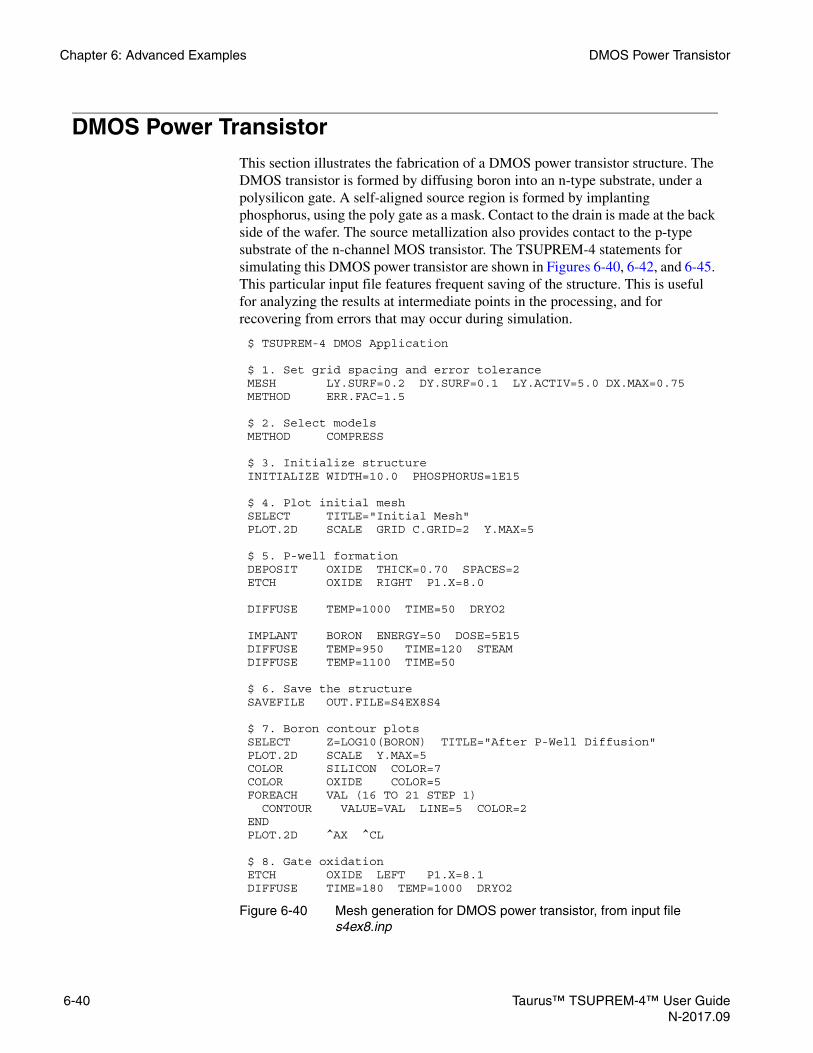
Chapter 6: Advanced Examples DMOS Power Transistor

DMOS Power TransistorThis section illustrates the fabrication of a DMOS power transistor structure. The DMOS transistor is formed by diffusing boron into an n-type substrate, under a polysilicon gate. A self-aligned source region is formed by implanting phosphorus, using the poly gate as a mask. Contact to the drain is made at the back side of the wafer. The source metallization also provides contact to the p-type substrate of the n-channel MOS transistor. The TSUPREM-4 statements for simulating this DMOS power transistor are shown in Figures 6-40, 6-42, and 6-45. This particular input file features frequent saving of the structure. This is useful for analyzing the results at intermediate points in the processing, and for recovering from errors that may occur during simulation.

$ TSUPREM-4 DMOS Application

$ 1. Set grid spacing and error toleranceMESH LY.SURF=0.2 DY.SURF=0.1 LY.ACTIV=5.0 DX.MAX=0.75METHOD ERR.FAC=1.5

$ 2. Select modelsMETHOD COMPRESS

$ 3. Initialize structureINITIALIZE WIDTH=10.0 PHOSPHORUS=1E15

$ 4. Plot initial meshSELECT TITLE="Initial Mesh"PLOT.2D SCALE GRID C.GRID=2 Y.MAX=5

$ 5. P-well formationDEPOSIT OXIDE THICK=0.70 SPACES=2ETCH OXIDE RIGHT P1.X=8.0

DIFFUSE TEMP=1000 TIME=50 DRYO2

IMPLANT BORON ENERGY=50 DOSE=5E15DIFFUSE TEMP=950 TIME=120 STEAMDIFFUSE TEMP=1100 TIME=50

$ 6. Save the structureSAVEFILE OUT.FILE=S4EX8S4

$ 7. Boron contour plotsSELECT Z=LOG10(BORON) TITLE="After P-Well Diffusion"PLOT.2D SCALE Y.MAX=5COLOR SILICON COLOR=7COLOR OXIDE COLOR=5FOREACH VAL (16 TO 21 STEP 1) CONTOUR VALUE=VAL LINE=5 COLOR=2ENDPLOT.2D ^AX ^CL

$ 8. Gate oxidationETCH OXIDE LEFT P1.X=8.1 DIFFUSE TIME=180 TEMP=1000 DRYO2

Figure 6-40 Mesh generation for DMOS power transistor, from input file s4ex8.inp

6-40 Taurus™ TSUPREM-4™ User GuideN-2017.09

DMOS Power Transistor Chapter 6: Advanced Examples

Mesh Generation

This simulation uses automatic grid generation and adaptive gridding. The automatic grid generation parameters have been adjusted to accommodate this large-geometry power device. The depth and spacing of the surface region (LY.SURF and DY.SURF, respectively) have been doubled and the depth of the active region (DY.ACTIV) has been increased from 4 to 5 microns.

A maximum horizontal grid spacing of DX.MAX=0.75 is used for this large-geometry device. The error factor for adaptive gridding has been set to 1.5 to reduce the number of nodes and speed up the simulation. A plot of the initial mesh is shown in Figure 6-41.

Processing the DMOS Power Transistor

Processing of the DMOS structure starts with the deposition of 7000 Å of oxide. An opening in this oxide layer is then made and a thin oxide is grown on the exposed silicon. Boron is then implanted through the opening to form the p+ contact for the body of the transistor. After implantation, the structure is oxidized, and the boron is driven further with an inert diffusion step. The COMPRESS oxidation model is used throughout the simulation to simulate oxidation of nonplanar structures.

Figure 6-41 Initial grid for simulating DMOS power transistor

0.00 4.00 8.00Distance (µm)

Dis

tanc

e (µ

m)

4.00

0.00

2.00

Taurus™ TSUPREM-4™ User Guide 6-41N-2017.09

Chapter 6: Advanced Examples DMOS Power Transistor

The structure after the oxidation and p-well drive is shown in Figure 6-43. Note that some oxide growth has occurred underneath the thick oxide, but not as much as occurred where the original oxide was removed.

$ 9. Save the structureSAVEFILE OUT.FILE=S4EX8S5

$ 10. Print oxide thicknessSELECT Z=1PRINT.1D LAYERS X.VALUE=0

$ 11. Poly gate formationDEPOSIT POLY THICK=0.5 PHOS=1E20 SPACES=2ETCH POLY RIGHT P1.X=4

$ 12. Body formationETCH OXIDE START X=4.0 Y=-10ETCH OXIDE CONT X=4.0 Y=10ETCH OXIDE CONT X=7.9 Y=10ETCH OXIDE END X=7.9 Y=-10

DIFFUSE TIME=40 TEMP=1000 DRYO2

IMPLANT BORON DOSE=5E14 ENERGY=70DIFFUSE TIME=60 TEMP=950 DRYO2DIFFUSE TIME=200 TEMP=1100

$ 13. Save the structureSAVEFILE OUT.FILE=S4EX8S6

Figure 6-42 Second part of file s4ex8.inp: Processing of DMOS power transistor, through body diffusion

Figure 6-43 Structure with contours of boron concentration, after first p-well diffusion

0.00 4.00 8.00Distance (µm)

Dis

tanc

e (µ

m)

4.00

0.00

2.00

6-42 Taurus™ TSUPREM-4™ User GuideN-2017.09

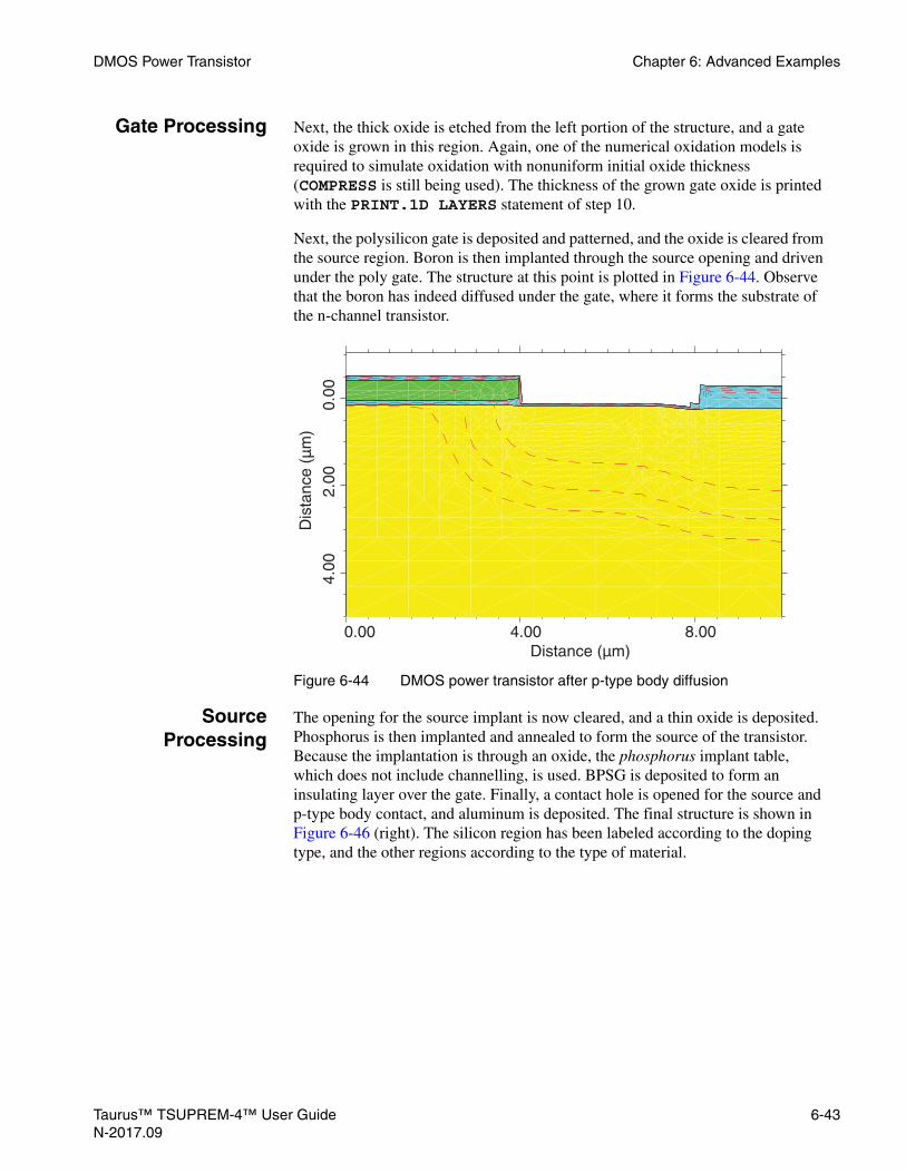
DMOS Power Transistor Chapter 6: Advanced Examples

Gate Processing Next, the thick oxide is etched from the left portion of the structure, and a gate oxide is grown in this region. Again, one of the numerical oxidation models is required to simulate oxidation with nonuniform initial oxide thickness (COMPRESS is still being used). The thickness of the grown gate oxide is printed with the PRINT.1D LAYERS statement of step 10.

Next, the polysilicon gate is deposited and patterned, and the oxide is cleared from the source region. Boron is then implanted through the source opening and driven under the poly gate. The structure at this point is plotted in Figure 6-44. Observe that the boron has indeed diffused under the gate, where it forms the substrate of the n-channel transistor.

SourceProcessing

The opening for the source implant is now cleared, and a thin oxide is deposited. Phosphorus is then implanted and annealed to form the source of the transistor. Because the implantation is through an oxide, the phosphorus implant table, which does not include channelling, is used. BPSG is deposited to form an insulating layer over the gate. Finally, a contact hole is opened for the source and p-type body contact, and aluminum is deposited. The final structure is shown in Figure 6-46 (right). The silicon region has been labeled according to the doping type, and the other regions according to the type of material.

Figure 6-44 DMOS power transistor after p-type body diffusion

0.00 4.00 8.00Distance (µm)

Dis

tanc

e (µ

m)

4.00

0.00

2.00

Taurus™ TSUPREM-4™ User Guide 6-43N-2017.09

Chapter 6: Advanced Examples DMOS Power Transistor

$ 14. Boron contour plotsSELECT Z=LOG10(BORON) TITLE="After Body Diffusion"PLOT.2D SCALE Y.MAX=5COLOR SILICON COLOR=7COLOR OXIDE COLOR=5COLOR POLY COLOR=3FOREACH VAL (16 TO 21 STEP 1) CONTOUR VALUE=VAL LINE.TYP=5 COLOR=2ENDPLOT.2D ^AX ^CL

$ 15. Source/drain formationETCH OXIDE START X=4.1 Y=-10ETCH OXIDE CONT X=4.1 Y=10ETCH OXIDE CONT X=7.9 Y=10ETCH OXIDE END X=7.9 Y=-10

DEPOSIT OXIDE THICK=0.03

IMPLANT PHOS DOSE=1E15 ENERGY=50 IMPL.TAB=PHOSPHORUSDIFFUSE TEMP=950 TIME=60 DRYO2

$ 16. BPSG and metallizationDEPOSIT OXIDE THICK=1.00 DIFFUSE TEMP=950 TIME=60 ETCH OXIDE RIGHT P1.X=6

DEPOSIT ALUMINUM THICK=1.5$ 17. Save the structureSAVEFILE OUT.FILE=S4EX8S7 $ 18. Plot final meshSELECT TITLE="Final Mesh"PLOT.2D SCALE GRID C.GRID=2 Y.MAX=5

$ 19. Boron and phosphorus contour plotsSELECT Z=LOG10(BORON) TITLE="Final structure"PLOT.2D SCALE Y.MAX=5COLOR SILICON COLOR=7COLOR OXIDE COLOR=5COLOR POLY COLOR=3COLOR ALUMINUM COLOR=2FOREACH VAL (16 TO 21 STEP 1) CONTOUR VALUE=VAL LINE.TYP=5 COLOR=2END

SELECT Z=LOG10(PHOS) FOREACH VAL (16 TO 21 STEP 1) CONTOUR VALUE=VAL LINE.TYP=4 COLOR=4END

PLOT.2D ^AX ^CL

LABEL X=9.8 Y=-0.5 LABEL="Aluminum" RIGHTLABEL X=1 Y=-0.9 LABEL="BPSG"LABEL X=1 Y=-0.1 LABEL="Poly"LABEL X=0.5 Y=1.5 LABEL="n-"LABEL X=9.8 Y=1.0 LABEL="p+" RIGHTLABEL X=3.1 Y=0.4 LABEL="p-"LABEL X=5.2 Y=0.4 LABEL="n+"

Figure 6-45 Third part of s4ex8.inp: Final processing and plotting

6-44 Taurus™ TSUPREM-4™ User GuideN-2017.09

DMOS Power Transistor Chapter 6: Advanced Examples

Figure 6-46 (left) shows the final grid for the structure. Observe that the mesh has been refined (automatically, by adaptive gridding) where needed to resolve the impurity profiles. Note that the grid refinement is primarily vertical in the center of the source region where the profiles are essentially one-dimensional, but occurs in both directions at the corners of the source diffusion, where 2-D effects are important.

The final structure is shown in Figure 6-46 (right).

Figure 6-46 Final mesh for DMOS simulation (left), showing the result of adaptive gridding, and final DMOS power transistor structure (right), produced by input file s4ex8.inp

Summary

The process shown here does not necessarily produce an ideal DMOS structure, nor is the simulation as accurate as it might be. Of particular importance are the conditions of the final drive of the p-type body diffusion in step 22 and the possibility that impurities may diffuse from the polysilicon gate through the gate oxide and into the channel. Observe in the final plot that there has apparently been some diffusion of both boron and phosphorus from the poly into the channel. Another concern is that oxidation-enhanced diffusion effects may be important in this example. This can be checked by repeating the simulation using the PD.TRANS point defect model.

0.00 5.00 10.00Distance (µm)

Dis

tanc

e (µ

m)

2.50

-2.5

0

Dis

tanc

e (µ

m)

2.50

-2.5

0

0.00 5.00 10.00Distance (µm)

BPSG

Poly

n–

n+p–

p+

Aluminum

Taurus™ TSUPREM-4™ User Guide 6-45N-2017.09

Chapter 6: Advanced Examples SOI MOSFET

SOI MOSFETThis example shows how TSUPREM-4 can be used to simulate a silicon-on-insulator (SOI) process. It illustrates several features of the program that have not been used in the other examples, including the use of the REGION statement and the technique for depositing layers with nonuniform grid spacings. The input statements from file s4ex9.inp are shown in Figures 6-47 and 6-49.

Mesh Generation

The structure to be simulated consists of a silicon wafer with a half micron of oxide and 0.2 microns of silicon on top. The active device is fabricated in the top silicon layer. The actual structure is formed by implantation of oxygen and recrystallization of the silicon layer on top, a process that cannot be simulated by TSUPREM-4. Instead, an initial structure is defined consisting of the silicon substrate and the oxide layer, on which the top silicon layer is deposited. Note that due to the symmetry of the final structure, only the left half needs to be simulated.

The silicon substrate and oxide layers are defined with LINE statements, as in previous examples. In this case, the TAG parameter must be added to grid lines on structure boundaries and material interfaces. Thus, in the y direction the tag OXTOP is used to mark the top of the oxide, OXBOTTOM to mark the oxide/silicon interface, and SIBOTTOM to mark the bottom of the structure. REGION

Figure 6-47 Mesh generation for SOI MOSFET, from input file s4ex9.inp

$ TSUPREM-4 SOI Structure (0.2um epi) Application $ Specify x meshLINE X LOCATION=0 SPACING=0.25 TAG=LEFTLINE X LOCATION=0.5 SPACING=0.025LINE X LOCATION=0.6 SPACING=0.025LINE X LOCATION=1.05 SPACING=0.1 TAG=RIGHT

$ Specify y meshLINE Y LOCATION=0 SPACING=0.02 TAG=OXTOPLINE Y LOCATION=0.5 SPACING=0.15 TAG=OXBOTTOMLINE Y LOCATION=2.0 SPACING=1.0 TAG=SIBOTTOM

ELIMINATE COLUMNS X.MIN=0.45 X.MAX=0.7 Y.MIN=0.05ELIMINATE COLUMNS Y.MIN=0.5

$ Define isolation oxide and silicon substrate REGION OXIDE XLO=LEFT XHI=RIGHT YLO=OXTOP YHI=OXBOTTOM REGION SILICON XLO=LEFT XHI=RIGHT YLO=OXBOTTOM YHI=SIBOTTOMINITIALIZE <100> BORON=1E15

$ Deposit epi with nonuniform vertical grid spacingDEPOSIT SILICON BORON=1E17 THICKNESS=0.1 SPACES=5 DY=0.01 YDY=0.1DEPOSIT SILICON BORON=1E17 THICKNESS=0.1 SPACES=5 DY=0.01

$ Plot initial meshSELECT Z=1 TITLE=”Initial Mesh”PLOT.2D GRID Y.MAX=1 SCALE C.GRID=2PRINT.1D X.VALUE=0.0 LAYERS

6-46 Taurus™ TSUPREM-4™ User GuideN-2017.09

SOI MOSFET Chapter 6: Advanced Examples

statements are added to identify the silicon and oxide regions. The REGION statements use the tags to specify the extent of the regions. Thus, for example, it is specified that the oxide region extends from the grid line tagged OXTOP to the line tagged OXBOTTOM, and from LEFT to RIGHT in the horizontal direction.

Depositing aLayer With

Nonuniform GridSpacing

The top silicon layer is added using DEPOSITION statements. To accurately simulate the final structure with the Medici device simulator, a fine grid spacing (about 100Å) is needed near each silicon/oxide interface. To reduce simulation time, a coarser grid is specified in the middle of the layer. Thus, the ideal mesh would have a spacing that varies smoothly from fine to coarse to fine.

A mesh of this type (shown in Figure 6-48) can be generated using the DY and YDY parameters on the DEPOSITION statement. The DY parameter specifies the desired grid spacing at some depth in the deposited layer specified by the YDY parameter. The grid spacing above and below this depth is increased or decreased to produce the specified number of spaces. To specify the grid spacing at two points in the layer (that is, at each interface), two DEPOSITION statements must be used. Each specifies a 1000Å layer of silicon divided into five grid spaces, as specified by the SPACES parameter.

In each case the DY parameter is used to specify the desired grid spacing of 0.01 microns. In the first case the 0.01-micron grid spacing occurs 0.1 microns below the top of the layer (that is, at the bottom of the layer), while in the second case the default value of YDY=0 is used, so the fine grid spacing occurs at the top of the layer. Note that the same mesh could have been generated by adding LINE and REGION statements to define the top silicon layer. The difficulty is that only a single doping concentration can be specified for the entire structure on the INITIALIZE statement, and it was necessary to specify a doping of 1017/cm3 in the top layer, but only 1015/cm3 in the lower layers.

Figure 6-48 Initial grid for simulating SOI MOSFET

0.00 0.50 1.00Distance (µm)

Dis

tanc

e (µ

m)

1.00

0.00

0.50

Taurus™ TSUPREM-4™ User Guide 6-47N-2017.09

Chapter 6: Advanced Examples SOI MOSFET

Figure 6-49 Processing of SOI MOSFET, from input file s4ex9.inp

$ Use vertical oxidation model to grow gate oxideDIFFUSE TIME=55 TEMP=950 DRYO2

SELECT Z=1PRINT.1D X.VALUE=0.0 LAYERS

$ Deposit, dope, and pattern polyDEPOSIT POLY THICK=0.3 SPACES=2METHOD COMPRESSDIFFUSE TIME=30 TEMP=800 PHOS=1E20ETCH POLY LEFT P1.X=0.5

$ Source/drain implant and annealIMPLANT ARSENIC DOSE=4E15 ENERGY=45DIFFUSE TIME=70 TEMP=950

$ BPSG and contact holesDEPOSIT OXIDE THICK=0.3DEPOSIT PHOTORESIST THICK=1.0ETCH PHOTORESIST LEFT P1.X=0.3ETCH OXIDE TRAP THICK=0.7 ANGLE=85ETCH PHOTORESIST ALL

$ MetallizationDEPOSIT ALUMINUM THICK=0.4DEPOSIT PHOTORESIST THICK=1.0ETCH PHOTORESIST RIGHT P1.X=0.6ETCH ALUMINUM TRAP THICK=0.7 ANGLE=85ETCH PHOTORESIST ALL

$ Reflect structure, then save complete MOSFETSAVEFILE OUT.FILE=S4EX9S1STRUCTURE REFLECT RIGHTSAVEFILE OUT.FILE=S4EX9P2 MEDICI

$ Plot grid & profiles for complete structureSELECT Z=DOPING TITLE=”SOI MOSFET”PLOT.2D SCALE Y.MAX=1COLOR SILICON COLOR=7COLOR OXIDE COLOR=5COLOR POLY COLOR=3COLOR ALUMINUM COLOR=2FOREACH X ( 16 TO 21 STEP 1 ) CONTOUR VALUE=( 10^ X ) COLOR=4 LINE.TYP=2 CONTOUR VALUE=(-(10^ X )) COLOR=2 LINE.TYP=5ENDPLOT.2D ^AX ^CL

PLOT.2D GRID SCALE Y.MAX=1 C.GRID=2

$ Plot 1D concentration profilesSELECT Z=LOG10(ACTIVE(BORON)) TITLE=”Doping Profiles” + LABEL=”log(Active Concentration)”PLOT.1D X.VALUE=1 BOTTOM=15 TOP=21 LEFT=-0.3 RIGHT=0 LINE.TYP=5 + COLOR=2LABEL LABEL=”Boron (x=1)” X=-0.1 Y=17

SELECT Z=LOG10(ACTIVE(ARSENIC))PLOT.1D X.VALUE=0 ^AXES ^CLEAR LINE.TYP=2 COLOR=3LABEL LABEL=”Arsenic (x=0)” X=-0.1 Y=20.3

6-48 Taurus™ TSUPREM-4™ User GuideN-2017.09

SOI MOSFET Chapter 6: Advanced Examples

Process Simulation

The processing of the SOI MOSFET is straightforward. Note that the analytical oxidation models cannot be used in this example, even though the surface is planar and unoxidized, because of the existence of the lower oxide/silicon interfaces.

The VERTICAL model can be used, but only because there is no path for oxygen to diffuse to the lower oxide layer, and thus no growth at the lower interfaces. If there were a path for oxygen to diffuse to the lower oxide, the COMPRESS or VISCOEL model would be needed, and if it were necessary to model lifting of the upper silicon layer, the VISCOUS model with SKIP.SIL set false would be needed.

Source/drain contacts have been opened and aluminum has been deposited and patterned to form contacts for Medici. The structure is reflected along the right edge to form a full device, and saved in Medici format in file S4EX9P2. The full, final structure is shown in Figure 6-50 on the left; the final grid is plotted in on the right.

Figure 6-50 Final structure, showing contours of net doping for SOI MOSFET (left) and final grid for SOI MOSFET (right)

0.00 1.00 2.00Distance (µm)

Dis

tanc

e (µ

m)

1.00

-1.0

00.

00

0.00 1.00 2.00Distance (µm)

Dis

tanc

e (µ

m)

1.00

-1.0

00.

00

Taurus™ TSUPREM-4™ User Guide 6-49N-2017.09

Chapter 6: Advanced Examples MOSFET With Self-Aligned Silicides

Figure 6-51 shows the doping profiles in the final structure. The arsenic profiles in the source/drain (x=0) and the boron profiles in the channel (x=1) are shown.

MOSFET With Self-Aligned SilicidesThis example illustrates the simulation of silicide growth using TSUPREM-4. The input files for this example are shown in Figures 6-52, 6-53, and 6-54. The statements are separated into two files—s4ex10.inp contains the processing statements for performing the simulation, while s4ex10p.inp contains the statements for plotting the structure.

Preparation for Silicidation

Figure 6-52 shows the statements used to initialize the structure, grow the gate oxide, deposit and pattern the poly gate, form the lightly doped source/drain extension and the heavily doped source/drain, and clear the oxide from the poly gate and the source/drain in preparation for silicidation. Automatic grid generation is used in both the vertical and horizontal directions, but because the structure is very small it is appropriate to reduce the depth of the active region and the grid space is provided automatically by adaptive gridding.

Figure 6-51 Channel and source/drain doping profiles for SOI MOSFET

-0.30 -0.20 0.00Distance (µm)

log(

Act

ive

Con

cent

ratio

n)

-0.10

21

20

19

18

17

16

15

Arsenic (x=0)

Boron (x=1)

6-50 Taurus™ TSUPREM-4™ User GuideN-2017.09

MOSFET With Self-Aligned Silicides Chapter 6: Advanced Examples

Silicidation

Figure 6-53 shows the statements for growing the self-aligned titanium silicide layer. First, titanium is deposited over the entire structure. Where titanium comes into contact with silicon or polysilicon, a thin (2 nm, by default) layer of TiSi2 is inserted automatically by the program. The structure after titanium deposition is shown in Figure 6-55. The next step is to anneal for a little over a minute at 650 degrees. Because it is expected that impurity diffusion is negligible, the PD.FERMI model is selected to reduce the simulation time.

During silicide growth, silicon atoms enter the silicide layer and diffuse to the TiSi2/Ti interface where they react to form more TiSi2. Silicon and titanium are consumed at their respective interfaces with the silicide, and silicide is formed at the TiSi2/Ti interface. The deformation of the various layers due to the consumption of silicon and titanium and the production of titanium silicide is calculated using the COMPRESS model for viscous flow.

Figure 6-52 First part of input file s4ex10.inp: NMOS transistor processing

$ TSUPREM-4 Silicidation Example

MESH GRID.FAC=0.9

MESH DY.SURF=0.03 LY.ACTIV=0.5 DY.ACTIV=0.1INITIALIZE BORON=1.0E15 WIDTH=0.6 DX=0.1

$ Grow gate oxideDIFFUSION TIME=25 TEMP=850 HCL=4.5 DRYO2

$ Deposit and pattern gateDEPOSIT POLYSILI THICKNES=0.2 SPACES=5 DY=0.02ETCH POLYSILI RIGHT P1.X=0.125ETCH OXIDE RIGHT P1.x=0.125

$ OxidizeMETHOD COMPRESSDIFFUSION TIME=25 TEMP=850 HCL=4.5 DRYO2

$ LDD implantIMPLANT ARSENIC DOSE=5E13 ENERGY=30 IMPL.TAB=ARSENIC

$ Form sidewall spacerDEPOSIT OXIDE THICKNESS=0.126 SPACES=2ETCH OXIDE TRAPEZOI THICKNESS=0.175

$ Heavy source/drain implant and annealIMPLANT ARSENIC DOSE=1E15 ENERGY=60 IMPL.TAB=ARSENICMETHOD PD.TRANSDIFFUSION TIME=10 TEMP=900 DRYO2

$ Isotropic etch to clear gate and source/drainETCH OXIDE TRAP THICK=0.015 ANGLE=45

Taurus™ TSUPREM-4™ User Guide 6-51N-2017.09

Chapter 6: Advanced Examples MOSFET With Self-Aligned Silicides

Figure 6-53 Second part of input file s4ex10.inp: Silicide growth

$ Deposit titaniumDEPOSIT MAT=TITANIUM THICK=0.025 SPACES=2

$ Plot structure before silicidationSELECT TITLE=”Before Silicidation”SOURCE s4ex10p.inp

$ Grow the silicideMETHOD PD.FERMIDIFFUSION TIME=1.287 TEMP=650

$ Plot structure after silicidationSELECT TITLE=”After Silicidation”SOURCE s4ex10p.inp

$ Final structureETCH MAT=TITANIUM ALLSTRUCTURE REFLECT LEFT

$ Plot structure after silicidationSELECT TITLE=”After Titanium Etch”SOURCE s4ex10p.inp

$ Print layer informationSELECT Z=DOPINGPRINT.1D X.V=0.6 LAYERSPRINT.1D X.V=0.0 LAYERS

Figure 6-54 Input file se4ex10p.inp: Plotting results

$ Plot sequence for silicidation example$$ To use:$ select title=”Title”$ source s4ex10p.inp$PLOT.2D Scale Y.MAX=0.3COLOR MAT.POLY COLOR=3SELECT Z=LOG10(ARSENIC)FOREACH X ( 15 TO 20 )

CONTOUR VAL=@{X} COLOR=3 LINE=3ENDCOLOR MAT=TITANIUM COLOR=2COLOR MAT=TISI2 COLOR=6COLOR MAT=OXIDE COLOR=5LABEL X=0.36 Y=-0.23 SIZE=0.3 RECT C.RECT=2 LABEL=”Titanium”LABEL X=0.36 Y=-0.18 Size=0.3 Rect C.RECT=6 LABEL=”TiSi2”LABEL X=0.36 Y=-0.13 SIZE=0.3 RECT C.RECT=3 LABEL=”Polysilicon”LABEL X=0.36 Y=-0.08 Size=0.3 Rect C.RECT=5 LABEL=”Oxide”LABEL X=0.55 Y=0.25 Size=0.3 Line=3 C.LINE=3 LABEL=”Arsenic” RIGHTPLOT.2D ^AX ^CL

6-52 Taurus™ TSUPREM-4™ User GuideN-2017.09

MOSFET With Self-Aligned Silicides Chapter 6: Advanced Examples

The structure after the silicide growth step is shown in Figure 6-56. Observe that most of the titanium has been consumed. After removing the remaining titanium the full structure is shown in Figure 6-57.

Figure 6-55 Structure immediately before silicide growth step

Figure 6-56 Structure after silicide growth step

0.00 0.20 0.60Distance (µm)

Dis

tanc

e (µ

m)

0.20

-0.2

00.

00

0.40

Titanium

TiSi2

Polysilicon

Oxide

Arsenic

0.00 0.20 0.60Distance (µm)

Dis

tanc

e (µ

m)

0.20

-0.2

00.

00

0.40

Titanium

TiSi2

Polysilicon

Oxide

Arsenic

Taurus™ TSUPREM-4™ User Guide 6-53N-2017.09

Chapter 6: Advanced Examples Polysilicon Emitter Study

Polysilicon Emitter StudyThis example shows a simulation of the emitter region of a double-polysilicon bipolar transistor. The effect of the arsenic out-diffusion from the emitter polysilicon on the emitter and base widths is shown. The simulations can be used to examine the dependence of the device performance on the width of the emitter stripe. The advanced polysilicon grain-growth and diffusion models are used to simulate the distribution of arsenic in the emitter.

Process Simulation

Figure 6-58 shows the input file s4ex11a.inp for simulating the emitter region of the bipolar transistor. The emitter width is defined by the name EMITWID. The input file s4ex11b.inp for simulating the 2-micron emitter is identical except for the values of IDENT (which is set to “B”) and the value of EMITWID which is set to 2.0.

The critical dimensions of the structure are specified by defining the parameters EMITSTA, EMITWID, and SPACERWID. The grid spacings are set to give a reasonable compromise between speed and accuracy. Adaptive gridding is used to increase the grid density where the arsenic diffuses to form the emitter; because of the shallowness of the emitter, the minimum grid spacing for adaptive gridding on arsenic is decreased to 0.01 micron. The accuracy of the results can be verified by reducing the value of GRID.FAC for later simulations.

Models Because oxidation-enhanced of transient-enhanced diffusion are not expected to be significant in this structure, the PD.FERMI diffusion model can be used with a shallow simulation structure. Because of the high arsenic concentration in the emitter, however, it would be wise to check the results using the PD.FULL model and a deep simulation structure.

Figure 6-57 Final structure, after removal of remaining titanium

-0.50 -0.25 0.25Distance (µm)

Dis

tanc

e (µ

m)

0.25

-0.2

50.

00

0.00

Titanium

TiSi2Polysilicon

Oxide

Arsenic

0.50

6-54 Taurus™ TSUPREM-4™ User GuideN-2017.09

Polysilicon Emitter Study Chapter 6: Advanced Examples

Processing The emitter structure is formed by a series of deposition and etch steps, culminating in the deposition of the poly layer in the trench formed by the emitter opening. The temperature of the poly deposition is 620°C; this temperature determines the initial grain size. The emitter is then implanted with arsenic at a 7-degree tilt. Because of the tilt, the right sidewall of the emitter receives more of the implant dose than the left sidewall, but much less than the bottom of the emitter opening. The arsenic is then diffused throughout the poly and into the single-crystal silicon with a high-temperature RTA step.

Taurus™ TSUPREM-4™ User Guide 6-55N-2017.09

Chapter 6: Advanced Examples Polysilicon Emitter Study

Figure 6-58 Listing of input file s4ex11a.inp for simulating the bipolar emitter structure

$ Parameters%DEFINE IDENT A%DEFINE EMITSTA 0.5%DEFINE EMITWID 1.0%DEFINE SPACERWID 0.2

$ Half the structureMESH GRID.FAC=1.5

LINE X LOC=0.0 SPACING=0.2LINE X LOC=@{EMITSTA}+@{SPACERWID}/2 SPACING=0.05LINE X LOC=@{EMITSTA}+@{EMITWID}/2 SPACING=0.15LINE Y LOC=0.0 SPACING=0.025LINE Y LOC=0.1 SPACING=0.025LINE Y LOC=1.0 SPACING=0.1ELIMINATE COLUMNS Y.MIN=0.2ELIMINATE COLUMNS Y.MIN=0.2INITIAL <100> BORON=1E14

METHOD MAT=SILICON IMP=ARSENIC MIN.SPAC=0.01

$ Emitter CutDEPOSIT OXIDE THICK=0.6 DY=0.05ETCH OXIDE RIGHT P1.X=@{EMITSTA}

$ Dielectric Screening LayersDEPOSIT OXIDE THICK=0.04 SPACES=2DEPOSIT NITRIDE THICK=0.05 SPACES=2

$ SpacerETCH NITRIDE RIGHT P1.X=@{EMITSTA}+@{SPACERWID}

$ Oxide dipETCH OXIDE TRAPEZ THICK=0.06 UNDERCUT=0.06

$ Build Full StructureSTRUCTUR REFLECT RIGHT

$ N-polyDEPOSIT POLYSILI THICK=0.22 ARC.SPAC=0.05 DY=0.02 TEMPERAT=620

$ N+ implantIMPLANT DOSE=1.0E+16 ENERGY=50 ARSENIC TILT=7.0

SAVE OUT.FILE=S4EX11@{IDENT}S1

$ Emitter drive-inDIFFUSIO TEMPERAT=1125. TIME=0.5 NITROGEN

SAVE OUT.FILE=S4EX11@{IDENT}S2

6-56 Taurus™ TSUPREM-4™ User GuideN-2017.09

Polysilicon Emitter Study Chapter 6: Advanced Examples

Plotting the Results

The results are now plotted for the following structures:

• After Implant

• Doping and Grain Size

• Doping versus Stripe Width

After Implant Figure 6-59 shows the layers of the structure and the arsenic concentration in the poly immediately after the implant. This figure and the following figures were plotted using the input file s4ex11c.inp, which illustrates techniques for producing multiple plots on a single screen and for annotating shaded contour plots. The first part of s4ex11c.inp is shown in Figure 6-60.

Figure 6-59 Bipolar emitter structure and as-implanted arsenic profiles, as plotted using s4ex11c.inp

0.00 1.00Distance (µm)

Dis

tanc

e (µ

m)

-1.0

00.

00

2.00D

ista

nce

(µm

)

-1.0

00.

000.00 1.00

Distance (µm)2.00

PolyOxideNitride

1E16 cm−3 1E21

Poly Emitter Wide=1.0 Arsenic: As-Implanted

Taurus™ TSUPREM-4™ User Guide 6-57N-2017.09

Chapter 6: Advanced Examples Polysilicon Emitter Study

Doping andGrain Size

Figure 6-61 shows the total arsenic concentration and the poly grain size after the RTA step. The arsenic concentration is largest at the left and right edges of the structure, where the initial doping is high and the arsenic is confined to the poly layer by the underlying nitride layer. The concentration is lowest in the sidewalls of the emitter opening, where the as-implanted doping is low. The concentration at the center of the emitter opening is lower than that at the left and right edges of the structure because of diffusion into the sidewalls of the opening and into the single-crystal silicon. The rate of grain growth during high-temperature processing depends strongly on the doping concentration; thus the final contours of grain size are similar to the final contours of total arsenic concentration.

Figure 6-60 First part of s4ex11c.inp, for plotting the structure and contours of as-implanted arsenic concentration

$ Parameters for plot size and placement%define YMAX 0.5%define YLEN 5.8%define XOFF1 1.5%define XOFF2 10.8%define LSIZ 0.3%define TSIZ 0.35

$ As-implanted structureinitial in.file=S4EX11AS1

$ Plot structureselect title=”Poly Emitter Width=1.0”plot.2d scale y.max=@{YMAX} x.off=@XOFF1 y.len=@YLEN + t.siz=@TSIZ x.siz=@LSIZ y.siz=@LSIZcolor poly color=3color oxide color=5color nitride color=4label label=”Poly” c.rect=3 size=0.25 x=0.3 y=0.2label label=”Oxide” c.rect=5 size=0.25 x=0.3 y=0.3label label=”Nitride” c.rect=4 size=0.25 x=0.3 y=0.4plot.2d ^ax ^cl

$ Plot as-imlanted arsenicselect z=log10(arsenic) title=”Arsenic: As-Implanted”plot.2d scale y.max=@{YMAX} ^cl x.off=@XOFF2 y.len=@YLEN + t.siz=@TSIZ x.siz=@LSIZ y.siz=@LSIZ%define TOP 1E21%define BOTT 1E16%define INC (log10(@{TOP})-log10(@{BOTT}))/10foreach I (0 to 10) color min.value=(log10(@{BOTT}) + @{INC}*( I )) + max.value=(log10(@{BOTT}) + @{INC}*( I +1)) + color=(18- I ) label rectangle c.recta=(18- I ) c.siz=0.25 + x=(@{XOFF2}+2.6+0.25*( I )) y=2.5 cmendlabel label=”@{BOTT}” c.siz=0.2 x=@{XOFF2}+2.1 y=2.75 cmlabel label=”cm^-3 @{TOP}” c.siz=0.2 x=@{XOFF2}+3.5 y=2.75 cmplot.2d ^ax ^cl

6-58 Taurus™ TSUPREM-4™ User GuideN-2017.09

SiGe HBT Process Chapter 6: Advanced Examples

Doping VersusStripe Width

The depletion of the arsenic in the center of the emitter opening is a strong function of the width of the emitter stripe. Figure 6-62 compares the net doping for a 2-micron emitter stripe with that for a 1-micron stripe. For the 2-micron stripe, the doping in the poly across the width of the emitter opening is much higher. It can also be observed that more arsenic has diffused from the poly into the single-crystal silicon; the 2-micron emitter stripe produces a wider emitter and a narrower base than the 1-micron emitter stripe.

SiGe HBT ProcessThis application presents a complete process flow of making a SiGe HBT device. It illustrates how to use TSUPREM-4 USEIT to introduce SiGe related advanced models and how to compute lattice mismatch strain and stress. Within this example, strain and germanium trap effects on boron diffusion are considered. The carbon interstitial trap effect is also taken into consideration.

Figure 6-61 Contours of total arsenic concentration and poly grain size after RTA

0.00 1.00Distance (µm)

Dis

tanc

e (µ

m)

-1.0

00.

00

2.00

Dis

tanc

e (µ

m)

-1.0

00.

00

0.00 1.00Distance (µm)

2.00

4E19 cm−3 4E20

Total Arsenic Grain Size

0.001 µm 0.2

Figure 6-62 Contours of net doping for 1-micron and 2-micron emitter stripes

0.00 1.00Distance (µm)

Dis

tanc

e (µ

m) -1.0

00.

00

2.00

Dis

tanc

e (µ

m)

-1.0

00.

00

0.00 1.00Distance (µm)

2.00

3E19 cm−3 3E20

Net Doping Net Doping

3E19 cm−3 3E20

3.00

Taurus™ TSUPREM-4™ User Guide 6-59N-2017.09

Chapter 6: Advanced Examples SiGe HBT Process

Initial Structure and Collector Region Generation

The input statements for generating the initial structure are listed in Figure 6-63.

$ This example shows how to use USEIT to define Boron diffusion$ model in SiGe considering the effects of Germanium induced $ strain/stress, or Germanium traps, and also the model of $ carbon-interstitial traps.

$ TSUPREM-4: SiGe HBT Application

$ Set device structure control parametersassign name=width n.val=0.7assign name=bwidth n.val=0.4assign name=ewidth n.val=0.2

$ Mesh and initializemesh grid.fac=1 dx.max=0.5 dx.min=0.4 dx.ratio=1.5 + ly.surf=0.2 dy.surf=0.1 ly.active=8 dy.active=1 + ly.bot=8 dy.bot=1.5 dy.ratio=2 fastinit <100> impurity=boron I.resist=30 resistiv width=@width

$ Modelsmethod pd.trans viscoela imp.adap dif.adap ^ox.adap

$ Buried Arsenic implantdeposit oxide thick=0.03implant arsenic dose=5e+15 energy=200

$ Nburied_drivediff temp=600 time=50 t.fin=1150 f.N2=10 f.O2=0.2diff temp=1150 time=120 f.N2=10 f.O2=0.2diff temp=1150 time=50 t.fin=800 f.N2=10 f.O2=0.2diff temp=800 time=30

$ Epi si and pad oxideetch oxide alldeposit silicon thick=0.5 space=10 boron=1e15deposit oxide thick=0.03

$ Ncollector implantimplant phos dose=5e+13 energy=200

$ N collector driveetch oxide alldiff time=15 temp=800 t.fin=950 dryO2diff time=10 temp=950 dryO2diff time=30 temp=950 t.fin=800

$ Etch sietch oxide allextract name=top silicon x=0 dist=0 y.ext ^write assignassign name=ySi n.val=@top+0.25etch silicon right p1.x=@bwidth p2.y=@ySi

$ Fill oxidedeposit oxide thick=0.4 space=3

$ Etchextract name=top silicon x=0 dist=0 y.ext ^write assignassign name=ytop1 n.val=@top-0etch oxide start x=0 y=-10etch cont x=0 y=@ytop1etch cont x=10 y=@ytop1

6-60 Taurus™ TSUPREM-4™ User GuideN-2017.09

SiGe HBT Process Chapter 6: Advanced Examples

etch cont x=10 y=-10etch done x=0 y=-10

A coarse mesh is first generated for the silicon wafer with boron impurity. Several build-in models are then selected for impurity diffusion, deformation evolution, and adaptive meshing. The next steps generate the buried collector region.

Using SiGe-Related Models

The next three SOURCE statements include USEIT files that define the SiGe data, the model for computing lattice mismatch strain and stress, the model for boron diffusion with strain effect and germanium/carbon trap effect.

They are Ge-in-Si.data, sige-stress-trap.usit, and carbon.usit, as shown in Figure 6-64, Figure 6-65, and Figure 6-66.

Figure 6-63 First part of sige_hbt.inp, for generating initial structure and the collector region.

Taurus™ TSUPREM-4™ User Guide 6-61N-2017.09

Chapter 6: Advanced Examples SiGe HBT Process

$------ Germanium coefficients -----------$ USEIT SiGe diffusion model implementation - data for germanium in silicon$ most of the data is similar to arsenic

impurity new imp=germanium at.num=32 at.wt=72.61 + tif.name=Ge c.init=1E5 impl.tab=arsenicimpurity imp=germanium t.act.0=8e-16 t.act.e=-4.2 act.min=1 cm.secimpurity imp=germanium mater=silicon dix.0=0.037 dix.e=5.46 cm.secimpurity imp=germanium mater=silicon /mater=oxide seg.0=30 + seg.e=0.6 trans.0=0.1 trans.e=0impurity imp=germanium mat=TiSi2 cm.sec dix.0=4.0e-7 dix.e=1.8impurity imp=germanium /mat=TiSi2 seg.0=0.8 trans.0=1e6 trans.e=2.0impurity imp=germanium mat=poly /mat=TiSi2 seg.0=0.8 + trans.0=1e6 trans.e=2.0impurity imp=germanium mat=WSi2 dix.0=2.6e-2 dix.e=2.11 cm.secimpurity imp=germanium mat=silicon /mat=WSi2 seg.0=10 + seg.e=0.0 trans.0=3.0e-3 trans.e=0.0impurity imp=germanium mat=poly /mat=WSi2 seg.0=10 + seg.e=0.0 trans.0=3.0e-3 trans.e=0.0impurity imp=germanium mat=oxide dix.0 =1.05E10 dix.e =4.89impurity imp=germanium mat=nitride dix.0 =0.0 dix.e =0.0impurity imp=germanium mat=oxynitri dix.0 =0.0 dix.e =0.0impurity imp=germanium mat=ambient dix.0 =5.00e13 dix.e =3.95impurity imp=germanium mat=si /mat=poly seg.0=1.0 + seg.e=0. trans.0=0.1 trans.e=0.impurity imp=germanium mat=si /mat=oxid seg.0=30. + seg.e=0. trans.0=0.1 trans.e=0.impurity imp=germanium mat=si /mat=nit seg.0=1.0 + seg.e=0. trans.0=0.0 trans.e=0.impurity imp=germanium mat=si /mat=oxyn seg.0=1.0 + seg.e=0. trans.0=0.0 trans.e=0.impurity imp=germanium mat=si /mat=amb seg.0=1.0 seg.e=0. + trans.0=9.0E5 trans.e=1.99impurity imp=germanium mat=poly /mat=oxid seg.0=30. seg.e=0. + trans.0=0.1 trans.e=0.impurity imp=germanium mat=poly /mat=nit seg.0=1.0 seg.e=0. + trans.0=0.0 trans.e=0.impurity imp=germanium mat=poly /mat=oxyn seg.0=1.0 seg.e=0. + trans.0=0.0 trans.e=0.impurity imp=germanium mat=poly /mat=amb seg.0=1.0 seg.e=0. + trans.0=9.0E5 trans.e=1.99impurity imp=germanium mat=oxid /mat=nit seg.0=1.0 seg.e=0. + trans.0=0.0 trans.e=0.impurity imp=germanium mat=oxid /mat=oxyn seg.0=1.0 seg.e=0. + trans.0=0.0 trans.e=0.impurity imp=germanium mat=oxid /mat=amb seg.0=1.0 seg.e=0. + trans.0=9.0E5 trans.e=1.99impurity imp=germanium mat=nit /mat=oxyn seg.0=1.0 seg.e=0. + trans.0=0.0 trans.e=0.impurity imp=germanium mat=nit /mat=amb seg.0=1.0 seg.e=0. + trans.0=0.0 trans.e=0.impurity imp=germanium mat=oxyn /mat=amb seg.0=1.0 seg.e=0. + trans.0=0.0 trans.e=0.impurity imp=germanium mat=polysili cm.sec dix.0=1.14e-2 + dix.e=3.44method imp=germanium silicon abs.adap=1e14 rel.adap=0.2 + min.spac=0.025method imp=germanium poly abs.adap=1e15 rel.adap=0.3 + min.spac=0.03method imp=germanium oxide abs.adap=1e16 rel.adap=2.0 + min.spac=0.1

6-62 Taurus™ TSUPREM-4™ User GuideN-2017.09

SiGe HBT Process Chapter 6: Advanced Examples

$ USEIT file for B diffusion models in SiGe: Ge trapped boron, and/or $ self-consistant SiGe strain/stress, or fixed strain. These models$ are based on Lever et.al.’s work (“Boron diffusion across Si-SiGe$ boundaries”, JAP 83, 1988(1998)), and the work by Cowern et.al$ ( “Diffusion in Strained SiGe”, PRL 72, 2585(1994)).

$------ Germanium coefficients -----------$ USEIT SiGe diffusion model implementation - data for germanium in $ silicon most of the data is similar to arsenic $ source ./Ge-in-Si.data

$ Chose model of B diffusion in SiGe $ mod=mod1 consider Ge trap boron only$ mod=mod2 consider Ge induced fixed strain only$ mod=mod3 consider self-consistant SiGe strain/stress$ mod=mod4 consider both Ge trap and SiGe strain/stress

$ assign name=mod c.v=”mod1”; default mod=1

$ B diffusion model

intermed name=PoissR express=0.28intermed name=YoungM express=1.87e12intermed name=c1 express=0.5*(1-PoissR)/YoungMintermed name=c2 express=PoissR/YoungM

intermed name=GeMax express=5e22intermed name=StrainMax express=-0.042intermed name=GeFrac express=Germanium/GeMax

if (“@mod” == “mod2”) intermed name=StrainSiGe express=GeFrac*StrainMaxelseif ( (“@mod” == “mod3”) || (“@mod” == “mod4”) )intermed name=StrainSiGe express=c1*(Sxx+Szz)-c2*Syyelseintermed name=StrainSiGe express=0if.end

intermed name=EaStrain express=-17 ;$Boron dEa per unit strain intermed name=dEa express=EaStrain*StrainSiGeintermed name=DX0 expr=0.0368intermed name=DBE expr=3.46+dEaintermed name=DP0 expr=0.716intermed name=Db size=2 minindex=0 + expr=”DX0*exp(-DBE/kt),DP0*exp(-DBE/kt)”

intermed name=dEg express=0.7intermed name=Ni expr=3.87e16*exp(-0.605/kt+1.5*log(temp))intermed name=NiSiGe express=Ni*exp(GeFrac*dEg/(2*kt))intermed name=C0 express=3.2e21intermed name=fTrap express=1/(1.0+Germanium/C0)

intermed name=Na express=active(boron)intermed name=Nd express=active(arsenic)+active(phosphorus)intermed name=Nt express=(Na-Nd) intermed name=Q express=sqrt(Nt^2+4*NiSiGe^2)intermed name=nelectron express=0.5*(Q-Nt)intermed name=nhole express=0.5*(Q+Nt)

$pd.ferm for boron

Figure 6-64 USEIT file, Ge-in-Si.data, defining Ge parameters.

Taurus™ TSUPREM-4™ User Guide 6-63N-2017.09

Chapter 6: Advanced Examples SiGe HBT Process

$intermed name=DbSiGe express=Db[0]+Db[1]*nhole/Ni

$pd.trans for boronintermed name=fI express=0.95intermed name=DbSiGe + express=(Db[0]+Db[1]*nhole/Ni)*(fI*CI.RATIO+(1-fI)*CV.RATIO)

if ( (“@mod” == “mod2”) || (“@mod” == “mod3”) )intermed name=Bmobile express=active(boron)elseintermed name=Bmobile express=fTrap*active(boron)if.end

equation model=sige variable=boron mat=si + addtoexp=”div(DbSiGe*(grad(Bmobile)+ + Bmobile/Q*(grad(Nt)+2*nelectron*grad(log(NiSiGe)))))”

$ Turn off boron built-in model, turn on USEIT model impurity imp=boron mat=si ^diffusemethod model=sige enable init.time=1e-12

if ( (“@mod” == “mod3”) || (“@mod” == “mod4”) )method st.histo viscoela ^skip.silif.end

$ Set silicon intrin.s before SiGe deposition command

Figure 6-65 USEIT file, sige-stress-trap.usit, defining the model for boron diffusion with strain effect and Germanium trap effect.

6-64 Taurus™ TSUPREM-4™ User GuideN-2017.09

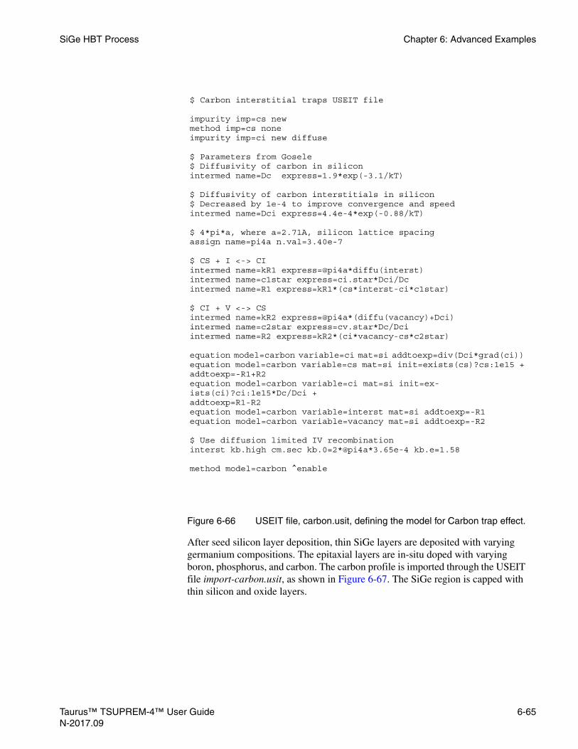
SiGe HBT Process Chapter 6: Advanced Examples

After seed silicon layer deposition, thin SiGe layers are deposited with varying germanium compositions. The epitaxial layers are in-situ doped with varying boron, phosphorus, and carbon. The carbon profile is imported through the USEIT file import-carbon.usit, as shown in Figure 6-67. The SiGe region is capped with thin silicon and oxide layers.

Figure 6-66 USEIT file, carbon.usit, defining the model for Carbon trap effect.

$ Carbon interstitial traps USEIT file

impurity imp=cs new method imp=cs noneimpurity imp=ci new diffuse

$ Parameters from Gosele$ Diffusivity of carbon in siliconintermed name=Dc express=1.9*exp(-3.1/kT)

$ Diffusivity of carbon interstitials in silicon$ Decreased by 1e-4 to improve convergence and speedintermed name=Dci express=4.4e-4*exp(-0.88/kT)

$ 4*pi*a, where a=2.71A, silicon lattice spacingassign name=pi4a n.val=3.40e-7

$ CS + I <-> CIintermed name=kR1 express=@pi4a*diffu(interst)intermed name=c1star express=ci.star*Dci/Dcintermed name=R1 express=kR1*(cs*interst-ci*c1star)

$ CI + V <-> CSintermed name=kR2 express=@pi4a*(diffu(vacancy)+Dci)intermed name=c2star express=cv.star*Dc/Dciintermed name=R2 express=kR2*(ci*vacancy-cs*c2star)

equation model=carbon variable=ci mat=si addtoexp=div(Dci*grad(ci))equation model=carbon variable=cs mat=si init=exists(cs)?cs:1e15 +addtoexp=-R1+R2equation model=carbon variable=ci mat=si init=ex-ists(ci)?ci:1e15*Dc/Dci +addtoexp=R1-R2equation model=carbon variable=interst mat=si addtoexp=-R1equation model=carbon variable=vacancy mat=si addtoexp=-R2

$ Use diffusion limited IV recombinationinterst kb.high cm.sec kb.0=2*@pi4a*3.65e-4 kb.e=1.58

method model=carbon ^enable

Taurus™ TSUPREM-4™ User Guide 6-65N-2017.09

Chapter 6: Advanced Examples SiGe HBT Process

$ Add 1e20 carbon to sige layer

intermed name=Cprofile expr=” y<@YtopC? 0.0: (y<@YbotC? 1e20: 0.0)”select z=Cprofileprint.1 x.v=0 out.file=mycarbon.profileprofile impurity=cs in.file=mycarbon.profile

When a SiGe layer is deposited on a relaxed Si seed layer, the lattice constant mismatch introduces an in-plane mismatch strain. This strain in turn introduces an intrinsic stress in the SiGe layer. In this example, the mismatch strain is computed according to Vegard’s law. TSUPREM-4 first checks the local germanium concentration and converts it to the mol fraction. According to Vegard’s law, in the absence of relaxation via dislocations, the in-plane strain stn is related to the Ge fraction x by stn = -0.042x. For a thin layer with top surface free, the intrinsic stress sts is related to the stn by sts = stn(1-pr)/ym where pr is the Poisson ratio and ym is the Young’s modulus. TSUPREM-4 then solves the stress equations to reach equilibrium.

Figure 6-67 USEIT file, import-carbon.usit, defining Carbon profile.

6-66 Taurus™ TSUPREM-4™ User GuideN-2017.09

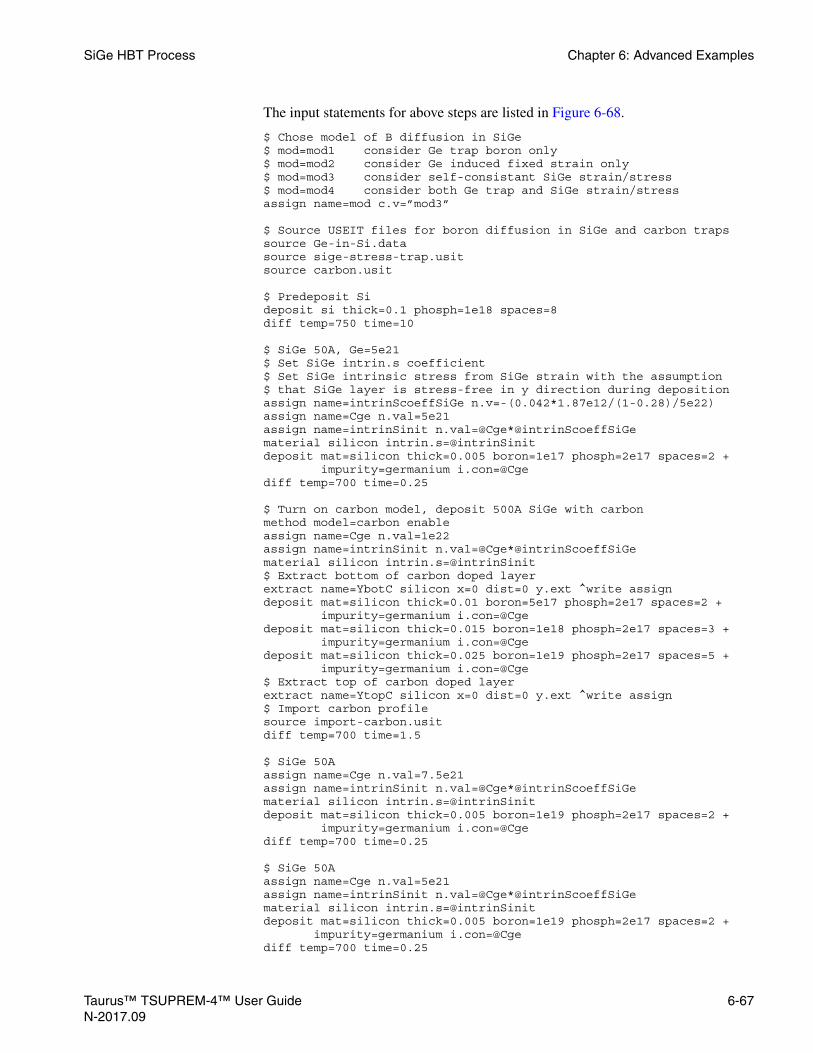
SiGe HBT Process Chapter 6: Advanced Examples

The input statements for above steps are listed in Figure 6-68.

$ Chose model of B diffusion in SiGe $ mod=mod1 consider Ge trap boron only$ mod=mod2 consider Ge induced fixed strain only$ mod=mod3 consider self-consistant SiGe strain/stress$ mod=mod4 consider both Ge trap and SiGe strain/stressassign name=mod c.v=”mod3”

$ Source USEIT files for boron diffusion in SiGe and carbon trapssource Ge-in-Si.datasource sige-stress-trap.usitsource carbon.usit

$ Predeposit Sideposit si thick=0.1 phosph=1e18 spaces=8diff temp=750 time=10

$ SiGe 50A, Ge=5e21$ Set SiGe intrin.s coefficient$ Set SiGe intrinsic stress from SiGe strain with the assumption$ that SiGe layer is stress-free in y direction during depositionassign name=intrinScoeffSiGe n.v=-(0.042*1.87e12/(1-0.28)/5e22)assign name=Cge n.val=5e21assign name=intrinSinit n.val=@Cge*@intrinScoeffSiGematerial silicon intrin.s=@intrinSinitdeposit mat=silicon thick=0.005 boron=1e17 phosph=2e17 spaces=2 + impurity=germanium i.con=@Cgediff temp=700 time=0.25

$ Turn on carbon model, deposit 500A SiGe with carbonmethod model=carbon enableassign name=Cge n.val=1e22assign name=intrinSinit n.val=@Cge*@intrinScoeffSiGematerial silicon intrin.s=@intrinSinit$ Extract bottom of carbon doped layerextract name=YbotC silicon x=0 dist=0 y.ext ^write assigndeposit mat=silicon thick=0.01 boron=5e17 phosph=2e17 spaces=2 + impurity=germanium i.con=@Cgedeposit mat=silicon thick=0.015 boron=1e18 phosph=2e17 spaces=3 + impurity=germanium i.con=@Cgedeposit mat=silicon thick=0.025 boron=1e19 phosph=2e17 spaces=5 + impurity=germanium i.con=@Cge$ Extract top of carbon doped layerextract name=YtopC silicon x=0 dist=0 y.ext ^write assign$ Import carbon profilesource import-carbon.usitdiff temp=700 time=1.5

$ SiGe 50Aassign name=Cge n.val=7.5e21assign name=intrinSinit n.val=@Cge*@intrinScoeffSiGematerial silicon intrin.s=@intrinSinitdeposit mat=silicon thick=0.005 boron=1e19 phosph=2e17 spaces=2 + impurity=germanium i.con=@Cgediff temp=700 time=0.25

$ SiGe 50Aassign name=Cge n.val=5e21assign name=intrinSinit n.val=@Cge*@intrinScoeffSiGematerial silicon intrin.s=@intrinSinitdeposit mat=silicon thick=0.005 boron=1e19 phosph=2e17 spaces=2 + impurity=germanium i.con=@Cgediff temp=700 time=0.25

Taurus™ TSUPREM-4™ User Guide 6-67N-2017.09

Chapter 6: Advanced Examples SiGe HBT Process

$ SiGe 50Aassign name=Cge n.val=2.5e21assign name=intrinSinit n.val=@Cge*@intrinScoeffSiGematerial silicon intrin.s=@intrinSinitdeposit mat=silicon thick=0.005 boron=1e19 phosph=2e17 spaces=2 + impurity=germanium i.con=@Cgediff temp=700 time=0.25

The in-plane stress Sxx distribution is shown in Figure 6-69.

Base and Emitter

On top of the strained SiGe layers, several deposition, etching, implantation and diffusion steps are performed to make the extrinsic base and emitter. The last steps in the flow fabricate the base and emitter contacts. The input statements for above steps are listed in Figure 6-70 and the top portion of the final structure is shown in Figure 6-71.

Figure 6-68 Second part of sige_hbt.inp, for using SiGe related models.

Figure 6-69 The in-plane stress Sxx distribution around SiGe region.

6-68 Taurus™ TSUPREM-4™ User GuideN-2017.09

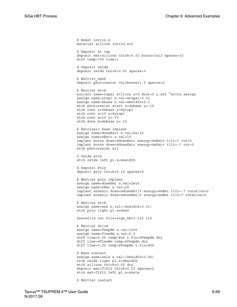
SiGe HBT Process Chapter 6: Advanced Examples

$ Reset intrin.smaterial silicon intrin.s=0

$ Deposit Si capdeposit mat=silicon thick=0.02 boron=1e12 spaces=10diff temp=750 time=1

$ Deposit oxidedeposit oxide thick=0.01 spaces=3

$ Emitter_maskdeposit photoresist thickness=1.5 spaces=2

$ Emitter etchextract name=topsi silicon x=0 dist=0 y.ext ^write assignassign name=ytop1 n.val=@topsi+0.01assign name=xbase n.val=@bwidth+0.1etch photoresist start x=@xbase y=-10etch cont x=@xbase y=@ytop1etch cont x=10 y=@ytop1etch cont x=10 y=-10etch done x=@xbase y=-10

$ Extrinsic base implantassign name=doseExtr n.val=5e+15assign name=eExtr n.val=15implant boron dose=@doseExtr energy=@eExtr tilt=7 rot=0implant boron dose=@doseExtr energy=@eExtr tilt=-7 rot=0etch photoresist all

$ Oxide etchetch oxide left p1.x=@ewidth

$ Deposit Polydeposit poly thick=0.15 spaces=5

$ Emitter poly implantassign name=doseEmi n.val=2e16assign name=eEmi n.val=20implant arsenic dose=@doseEmi/2 energy=@eEmi tilt=-7 rotation=0implant arsenic dose=@doseEmi/2 energy=@eEmi tilt=7 rotation=0

$ Emitter etchassign name=ew2 n.val=(@ewidth+0.01)etch poly right p1.x=@ew2

$savefile out.file=sige_hbt0.tif tif

$ Emitter driveassign name=TempEm n.val=1000assign name=TimeEm n.val=0.5diff time=0.05 temp=800 t.fin=@TempEm drydiff time=@TimeEm temp=@TempEm drydiff time=0.05 temp=@TempEm t.fin=800

$ Base contactassign name=xele n.val=(@bwidth+0.05)etch oxide right p1.x=@bwidthetch silicon thick=0.02 drydeposit mat=TiSi2 thick=0.02 spaces=2etch mat=TiSi2 left p1.x=@xele

$ Emitter contact

Taurus™ TSUPREM-4™ User Guide 6-69N-2017.09

Chapter 6: Advanced Examples SiGe HBT Process

extract name=toppoly poly x=0 dist=0 y.ext ^write assignassign name=ytop1 n.val=@toppoly+0.05etch oxide start x=0 y=-10etch cont x=0 y=@ytop1etch cont x=10 y=@ytop1etch cont x=10 y=-10etch done x=0.0 y=-10etch poly thick=0.05 drydeposition aluminum thickness=0.02etch aluminum right p1.x=@ewidth

$ Truncate bottomstructure truncate bot y=0.5

$ Rename contactassign name=xbase n.val=(@xele+0.02)extract name=topbase mat=TiSi2 X=@xbase dist=0 y.ext ^write assignassign name=ybase n.val=@topbase+0.01electrode X=@xbase Y=@ybase name=baseextract name=topEm aluminum x=0 dist=0 y.ext ^write assignassign name=yEm n.val=@topEm+0.01electrode X=0.05 Y=@yEm name=emitter

savefile out.file=sige_hbt.tif tif

Figure 6-70 Third part of sige_hbt.inp, for generating the base and emitter.

Figure 6-71 Top portion of the final SiGe HBT structure.

6-70 Taurus™ TSUPREM-4™ User GuideN-2017.09

CHAPTER 7

TN

User-Specified Equation Interface7

The User-Specified Equation Interface (USEIT) is an optionally available capability for TSUPREM-4 that helps you quickly develop and evaluate your own process models, without requiring the program to be recompiled and linked. USEIT supports Synopsys’ Physical Model and Equation Interface (PMEI) standard.

The chapter includes the following sections:

• Overview

• Using USEIT

• Examples

OverviewYou can use USEIT to specify model equations that have the general form:

at specified boundaries

where X is the quantity to be solved.

TSUPREM-4 assembles the matrices to solve equations by assuming that the time derivative term of X is placed at the left-hand-side (LHS) of the equation and all the other terms at the right-hand-side (RHS). To describe this equation using USEIT, any new terms that appear on the RHS of the equation are specified by the ADDTOEXP (alias ADD.RHS) parameter and the INTERFAC parameter on the EQUATION statement. The INTERFAC parameter is used to define the flux at interfaces.

The term Previous_RHS in the above expression represents terms that are already present on the RHS of the equation being modified. The initial condition of the variable X is specified with the INITIAL parameter or the IMPL.INI parameter in the EQUATION statement. The INTERMED statement specifies the intermediate quantities associated with equations.

X∂t∂

------ Previous_RHS ADDTOEXP INTERFAC+ +=

aurus™ TSUPREM-4™ User Guide 7-1-2017.09

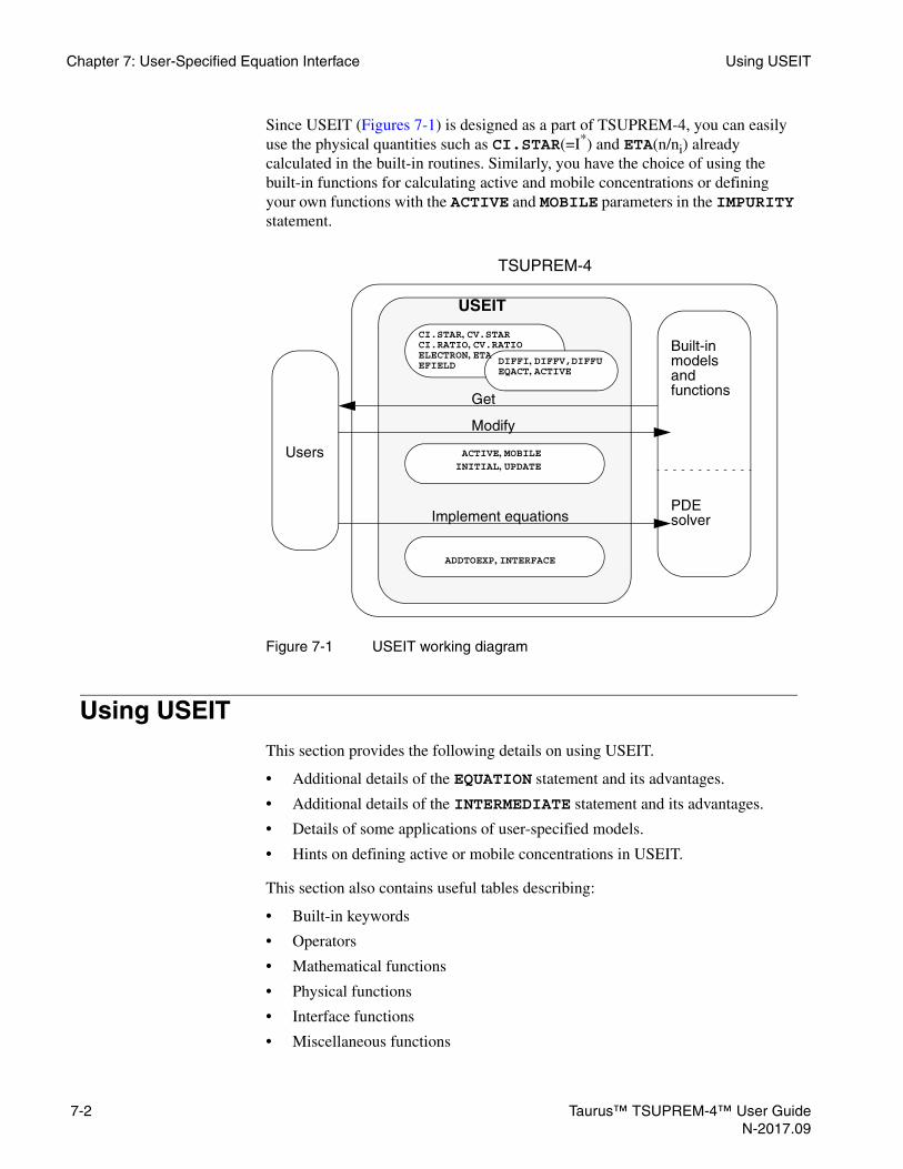
Chapter 7: User-Specified Equation Interface Using USEIT

Since USEIT (Figures 7-1) is designed as a part of TSUPREM-4, you can easily use the physical quantities such as CI.STAR(=I*) and ETA(n/ni) already calculated in the built-in routines. Similarly, you have the choice of using the built-in functions for calculating active and mobile concentrations or defining your own functions with the ACTIVE and MOBILE parameters in the IMPURITY statement.

Using USEITThis section provides the following details on using USEIT.

• Additional details of the EQUATION statement and its advantages.

• Additional details of the INTERMEDIATE statement and its advantages.

• Details of some applications of user-specified models.

• Hints on defining active or mobile concentrations in USEIT.

This section also contains useful tables describing:

• Built-in keywords

• Operators

• Mathematical functions

• Physical functions

• Interface functions

• Miscellaneous functions

Figure 7-1 USEIT working diagram

Get

Modify

Implement equations

DIFFI, DIFFV,DIFFUEQACT, ACTIVE

CI.STAR, CV.STARCI.RATIO, CV.RATIOELECTRON, ETAEFIELD

ACTIVE, MOBILE

ADDTOEXP, INTERFACE

Built-inmodelsandfunctions

PDEsolver

USEIT

TSUPREM-4

UsersINITIAL, UPDATE

7-2 Taurus™ TSUPREM-4™ User GuideN-2017.09

Using USEIT Chapter 7: User-Specified Equation Interface

EQUATION

The EQUATION statement is used to specify user-specified equations and is available only with the USEIT Option. See EQUATION, p. 4-233 for additional details.

New SolutionVariable

When a new solution variable is first specified in the EQUATION statement, it is automatically defined. A warning message is displayed explaining that the VARIABLE does not currently exist and is being defined. Alternatively, the solution variable can be defined in the IMPURITY statement with the NEW parameter. The following statement defines the new impurity BCL.

IMPURITY IMP=BCL NEW

Solving Method The METHOD statement specifies the numerical methods used to solve the equations. The factorization method of block matrices, the absolute, and the relative error tolerances for solutions should be specified. For example:

METHOD VARIABLE=RDL NONE ABS.ERR=0.1

where:

• RDL is a solution variable for dislocation-loop radius.

• The VARIABLE parameter is an alias for the IMPURITY parameter.

Since the RDL is supposed to be immobile, the factorization method is defined to NONE. The absolute error is set to 0.1. The unit of the absolute error is the same as the unit of the solution variable. The absolute error value is set to 1 x 109 by default, unless it is specified. Since the REL.ERR parameter is not specified, the relative error is set to 0.01, by default.

Initialization For solutions (for example, cluster) not introduced by external sources (such as implantation, predeposition, or epitaxy), the solution variable must be initialized to solve the partial differential equations. The INITIAL (alias: DIFF.INI) parameter or the IMPL.INI parameter in the EQUATION statement specifies the initial values of a solution variable in the specified.

The initialization by the INITIAL parameter is performed when the following conditions are satisfied:

• The solution variable has not yet been initialized before thermal processes (DIFFUSION or EPITAXY), or the solution variable was initialized and implantation was performed prior to thermal process.

• All other solution variables associated with the INITIAL expression are available, so that the INITIAL expression can be evaluated; or the solution variable is produced by reactions in the REACTION statement or the INTERFACE parameter in the EQUATION statement.

The parameter IMPL.INI defines the expression for the solution initialization at implant. The IMPL.INI expression is evaluated and applied at every implant step.

Taurus™ TSUPREM-4™ User Guide 7-3N-2017.09

Chapter 7: User-Specified Equation Interface Using USEIT

EQUATION VARIABLE=RDL MAT=Si +INIT="(1e20<inters+damage&&inters+damage<=1.15e22)?+ 300:(EXIST(RDL)?RDL:0.0)"

The example shows the initialization of the dislocation-loop radius. For additional details, see the Dislocation-Loop Model, p. 7-17.

IMPLANT ARSENIC DOSE=1E15 ENERGY=30 ;$1SELECT Z=RDL; PRINT.1D X.V=0 ;$2DIFFUSION TEMP=800 TIME=0 ;$3SELECT Z=RDL; PRINT.1D X.V=0 ;$4

In the second line, the RDL solution has not yet been initialized, so a warning message is displayed, explaining that RDL does not currently exist. The RDL is initialized at the third line, and then the spatial distribution of RDL is printed out at the fourth line.

Note:The intermediates in the INITIAL expression store the values at the previous thermal step. Thus, if the initialization includes the intermediates associated with the built-in point-defects, the initialization may be incorrect because the changes of the point-defect concentrations due to implants have not been reflected in the intermediates. For example:

The damage is zero at the previous thermal step, so that the Itotal stores the only interstitial concentration at the previous thermal step. Thus, the above initialization is incorrect. You can obtain the correct initialization by avoiding the use of INTERMED values in the INITIAL expression.

Example forInitialization

When DIFF.INI for interstitial is defined, the “total” interstitial concentration is reset to the values of the expression evaluated after regrowth. Then the “free” interstitial is calculated and stored to the interstitial solution. The example shows the method to initialize the interstitial concentration after regrowth. The example increases the interstitial concentration two times more than that of the implanted arsenic concentration.

First, the expression for the total interstitial concentration is described to the intermediate ITOT. The MYDAM and ASIMP intermediates store DAMAGE and DIMPLANT, respectively. DIMPLANT stores the newly added dopant concentration by implantation.

INTERMED NAME=Itotal VALUE=damage+interstEQUATION VARIABLE=RDL MAT=Si +

INIT="(1e20<Itotal&&Itotal<=1.15e22)? +LRAD:(EXIST(RDL)?RDL:0.0)"

7-4 Taurus™ TSUPREM-4™ User GuideN-2017.09

Using USEIT Chapter 7: User-Specified Equation Interface

$ DEFINE POINT-DEFECT MODEL AND MESHMETHOD PD.FULLMESH DY.SURF=0.001 DY.ACT=0.01 LY.ACT=0.5

$ DEFINE PARAMETERS FOR AMORPHOUS/CRYSTALLINE REGIONSASSIGN NAME=DAMGRAD N.V=10.0ASSIGN NAME=MAXDAM N.V=1.15E22ASSIGN NAME=DPLUS N.V=2.0

$ DEFINE SMOOTHING FACTOR AT A/C BOUNDARYINTERMED NAME=MYDAM EXPR=DAMAGEINTERMED NAME=ASIMP EXPR=DIMPLANTINTERMED NAME=EXPA + EXPR=EXP(@DAMGRAD*LOG(MYDAM/@MAXDAM))INTERMED NAME=EXPAM EXPR=1/EXPAINTERMED NAME=TANHA EXPR=(EXPA-EXPAM)/(EXPA+EXPAM)INTERMED NAME=FS EXPR=0.5-0.5*TANHAINTERMED NAME=ITOT EXPR=CI.STAR+FS*(@DPLUS*ASIMP)

The intermediate ITOT is assigned to DIFF.INI for interstitial in the EQUATION statement. Then arsenic implantation and 800oC zero time diffusion are given to show the interstitial profile after regrowth.

EQUATION MODEL=IEQINI IMP=INTERS MAT=SI DIFF.INI=ITOT

$ USE DIFF.INI FOR I INITIALIZATIONMETHOD MODEL=IEQINI ENABLEINITIMPLANT ARSENIC DOSE=1E15 ENERGY=20DIFFUSE TEMP=800 TIME=0SELECT Z=LOG10(INTERS)PLOT.1 X.V=0 TOP=21 BOT=15 RIGHT=0.5 COLOR=2

AddingExpressions to

Equations

The terms specified by the ADDTOEXP parameter in the EQUATION statement are added to the current right-hand-side (RHS) term of equations.

EQUATION VARIABLE=X MAT=Si +ADDTOEXP=DIV(dif*GRAD(X))

The above statement represents the following equation for the unknown X:

where Previous_RHS means the previously specified expressions or the built-in terms in the right-hand-side (RHS).

∂X∂t------ Previous_RHS ∇ dif X∇( )⋅+=

Taurus™ TSUPREM-4™ User Guide 7-5N-2017.09

Chapter 7: User-Specified Equation Interface Using USEIT

An additional specification of ADDTOEXP for the same solution variable in the same material adds the new expression to the previously specified terms; it does not replace the present expression with the new expression. For example:

EQUATION VARIABLE=X MAT=Si ADDTOEXP=expr1EQUATION VARIABLE=X MAT=Si ADDTOEXP=expr2

The final expression is the sum of expressions expr1 and expr2. You can replace the above statements with:

EQUATION VARIABLE=X MAT=Si ADDTOEXP=expr1+expr2

Flux at Interfaces The parameter INTERFAC in the EQUATION statement specifies the transport flux from material /MAT2 to material MAT1 at interfaces between the materials. The specified flux is added at the boundary nodes on the material MAT1. The parameter TRANSPOR specifies that the flux should also be subtracted at the boundary nodes on material /MAT2, so that the dose of the solution is conserved. The TRANSPOR parameter is turned on by default (see Figure 7-2).

$ B segregation at Si/OxINTERMED NAME=t VALUE=0.1*1E-4/60INTERMED NAME=m VALUE=1126*exp(-0.91/kt)EQUATION VARIABLE=BORON MAT1=Si /MAT2=Ox +

INTERFAC=t*(ONMAT2(BORON)-ONMAT1(BORON)/m)

The traditional segregation flux of boron between silicon and oxide is described. No specification of TRANSPOR implies that the flux must be subtracted on the boundary nodes in oxides.

The additional specification for the same solution variable on the same interface adds the new flux to the previously specified terms; it does not replace the present flux with the new flux. For example:

EQUATION VARIABLE=X MAT1=Si /MAT2=Ox INTERFAC=expr1EQUATION VARIABLE=X MAT1=Si /MAT2=Ox INTERFAC=expr2

The final flux is the sum of expressions expr1 and expr2. You can replace the above statements with:

EQUATION VAR=X MAT1=Si /MAT2=Ox INTERFAC=expr1+expr2

Diffusion AlongBoundaries

If the ADDTOEXP expression is specified with the BOUNDARY parameter in the EQUATION statement, the ADDTOEXP expression is applied only on the boundaries of MAT1, adjacent to /MAT2.

Figure 7-2 Flux at interfaces

MAT1 /MAT2

F

+F (-F when TRANSPOR is true)

A node on boundaries of MAT1A node on boundaries of /MAT2

F the flux specified by INTERFAC

7-6 Taurus™ TSUPREM-4™ User GuideN-2017.09

Using USEIT Chapter 7: User-Specified Equation Interface

$ Diffusion on the oxide surface along the Si/Ox.EQUATION VARIABLE=IBORON MAT1=Ox /MAT2=Si BOUNDARY +

ADDTOEXP=DIV(dif*GRAD(IBORON))

The expression in the ADDTOEXP parameter shows the diffusion along the boundaries of oxide adjacent to silicon.

Update Solution Use the parameter UPDATE in the EQUATION statement for the special case of updating the solution during solving equations. For example:

$ RDL : Dislocation loop radius (angstrom unit)EQUATION VARIABLE=RDL MAT=Si UPDATE=RDL>100?RDL:0.0

This example shows how to discard dislocation-loops with a radius of less than 100 angstroms. When solving the equation, the values of RDL less than 100 angstroms are set to zero.

INTERMEDIATE

The INTERMEDIATE statement (alias MODEL or ARRAY) specifies the intermediate quantities associated with equations. For additional details, see INTERMEDIATE, p. 4-30.

Advantages ofIntermediates

The advantages of using intermediates quantities are:

• Simplifying long and complicated equations

• Avoiding the duplicated calculation of quantities used in several equations

• Once the intermediates are evaluated, the calculated values are shared by all associated equations until the intermediates need to be reset.

• Avoiding duplicated calculation of quantities depending only on temperature

• If the intermediates depend only on temperature, they are evaluated only when the temperature changes.

• Using intermediates in the same manner as the built-in solution values in the SELECT statement.

Note:Intermediates are stored as symbolic expressions that are evaluated later (for example, when solving the model equations).

Application of User-Specified Models

The MODEL parameter controls the application of specified equations. By turning on/off the ENABLE parameter with the MODEL parameter in the METHOD statement, the equations grouped by the MODEL parameter in the IMPURITY and

Taurus™ TSUPREM-4™ User Guide 7-7N-2017.09

Chapter 7: User-Specified Equation Interface Using USEIT

REACTION statements can be enabled or disabled. The models not specified by the MODEL parameter are always turned on.

At process1, the equations in the model BIC are applied because it is turned on by default. Turning off the ENABLE parameter prior to process2 disables the BIC model. Simulate process3 with the BIC model by turning on the ENABLE parameter again.

The additional specification for the same solution variable in the same material or on the same interface with the same model name adds the new expression to the previously specified terms; it does not replace the present expression with the new expression. For example:

The final expression is the sum of expressions expr1 and expr2. You can replace the above statements with:

Specify the INITIAL, ACTIVE, MOBILE, and UPDATE parameters only once for the specified impurity and material in one model. The duplicated specification of these parameters for the same model replaces the previous definitions with the new ones. Even though it is possible for each different model to have its own INITIAL, ACTIVE, MOBILE, and UPDATE expressions, only one model among them should be enabled. Otherwise, incorrect results occur.

Modification of Built-in Functions

Define the modification of the active or mobile concentrations in USEIT using the following hints.

ACTIVE Usually, active concentrations are defined with the solid solubilities and the equilibrium clustering coefficients specified in the IMPURITY statement. When active concentrations need to be calculated differently, the ACTIVE parameter in the IMPURITY statement provides the new method to calculate active concentrations. The physical function ACTIVE() returns the values of active concentration calculated by the method that is specified in the ACTIVE parameter, while the ACTIVE parameter defines the calculation method itself for active concentration.

EQUATION MODEL=BIC VARIABLE=BORON MAT=Si ADDTOEXP=rhs1EQUATION MODEL=BIC VARIABLE=INTER MAT=Si ADDTOEXP=rhs2$ process1METHOD MODEL=BIC ^ENABLE$ process2METHOD MODEL=BIC ENABLE$ process3

EQUATION MODEL=mdl VARIABLE=X MATERIAL=m EXPR=expr1EQUATION MODEL=mdl VARIABLE=X MATERIAL=m EXPR=expr2

EQUATION MODEL=mdl VAR=X MAT=m EXPR=expr1+expr2

7-8 Taurus™ TSUPREM-4™ User GuideN-2017.09

Using USEIT Chapter 7: User-Specified Equation Interface

The Ceq and ni are defined as the equilibrium active boron concentration and intrinsic carrier concentration, respectively.

MOBILE In most cases, mobile concentrations are the same as active concentrations. However, when the mobile concentration is different from the active concentration, use the MOBILE parameter in the IMPURITY statement. For example, the diffusion retardation due to ion-pairing is described with the reduction of the mobile concentration.

The above equations are described using USEIT as follows:

Built-in Keywords

The following keywords are available.

IMPURITY IMP=BCL NEWINTERMED NAME=Ceq EXPRESS=EQACTIVE(boron,boron)INTERMED NAME=ni +

EXPRESS=3.87e16*exp(-0.605/kt+1.5*log(temp))IMPURITY IMP=boron MAT=Si +

ACTIVE=MAX(boron-BCL,MIN(Ceq,ni))

for acceptors, for donors

where

INTERMED NAME=ni +EXPR=3.87e16*exp(-0.605/kt+1.5*log(temp))

INTERMED NAME=Nd EXPR=ACTIVE(arsenic)+ACTIVE(phospho)INTERMED NAME=Na EXPR=ACTIVE(boron)INTERMED NAME=Nt EXPR=Nd+Na+6.0*niINTERMED NAME=Np EXPR=0.5*(Nt-sqrt(Nt*Nt-4*Nd*Na))INTERMED NAME=Fpa EXPR=1-Np/NaINTERMED NAME=Fpd EXPR=1-Np/NdIMPURITY MODEL=IONPAIR IMP=boro MAT=Si +

MOBILE=Fpa*ACTIVE(boron)IMPURITY MODEL=IONPAIR IMP=phos MAT=Si +

MOBILE=Fpd*ACTIVE(phos)IMPURITY MODEL=IONPAIR IMP=arse MAT=Si +

MOBILE=Fpd*ACTIVE(arse)

Cm 1Np

Na------–

Ca= Cm 1Np

Nd------–

Ca=

Np12--- Nd Na Ω+ +( ) Nd Na Ω+ +( )2

4NdNa––( )=

Name Type Value Unit

KB constant Boltzmann constant, J/oK

QE constant Electron charge, Coulomb

TEMP parameter Kelvin temperature oK

1.38066 1023–×

1.602 1019–×

Taurus™ TSUPREM-4™ User Guide 7-9N-2017.09

Chapter 7: User-Specified Equation Interface Using USEIT

Operators

The operators in higher tables have higher precedence than the operators in lower tables. expr means an expression.

KT parameter Thermal voltage, Volts

CI.STAR node solution Equilibrium interstitial concentration cm-3

CV.STAR node solution Equilibrium vacancy concentration cm-3

CI.RATIO node solution Ratio of interstitial concentrations to equilibrium None

CV.RATIO node solution Ratio of vacancy concentrations to equilibrium None

ELECTRON node solution Electron concentrationNote: Calculated by assuming local charge neutrality

cm-3

ETA node solution Electron concentration ratio to intrinsic carrier concentration None

EFIELD edge solution Electric field divided by thermal voltage cm-1

Name Type Value Unit

KB TEMP×

Name Type Value

^ expr ^ expr Power Example: CI.RATIO^2

+ +expr Unary positive

- -expr Unary negative

* expr * expr Multiply

/ expr /expr Divide

+ expr + expr Add

- expr - expr Subtract

> expr > expr Greater than

>= expr >= expr Greater than or equal to

< expr < expr Less than

<= expr <= expr Less than or equal to

== expr == expr Equal

!= expr != expr Not equal

&& expr && expr And

|| expr || expr Or

?: expr ? expr:expr condition_expression ? true_expression : false_expressionExample: BORON>PHOS?BORON:PHOSNote: Same as the CONDITION function. See Miscellaneous Functions, p. 7-14.

7-10 Taurus™ TSUPREM-4™ User GuideN-2017.09

Using USEIT Chapter 7: User-Specified Equation Interface

Mathematical Functions

The argument types, number, node value, and edge value in the argument list mean that the evaluation of the argument expressions results in number, node solution, and edge solution, respectively.

Function Argument List Return Value

LOG arg1 number or node value Natural logarithmic valueExample: LOG(10)Example: LOG(INTERST+DAMAGE)

LOG10 arg1 number or node value 10-based logarithmic value

EXP arg1 number or node value Exponential value

ERF arg1 number or node value Error function value

ERFC arg1 number or node value Complementary error function value

ABS arg1 number or node value Absolute value

SQRT arg1 number or node value Square root value

MIN arg1 number or node value:argN number or node valueNote: N must be larger than 1

Smallest valueExample: MIN(1,2,3)Example: MIN(BORON+PHOS,1E21)

MAX arg1 number or node value:argN number or node valueNote: N must be larger than 1

Largest valueExample: MAX(1,2,3)Example: MAX(BORON,PHOS+ARSENIC)

SUM arg1 indexarg2 numberarg3 numberarg4 number or node value

Summed value

Example: is described as

SUM(i,1,10,i^2)

Example: is described as

SUM(i,-2,2,SUM(j,0,5,k[i][j]))

SOLVE arg1 variable namearg2 expressionarg3 initial value

Extract the arg1’s value, which makes the expression equal to zero by Newton-Raphson iteration

Example: Extract x near 1.0 from the equation

SOLVE(x,x^2-3*x+1,1.0)

Example: Extract satisfying

INTERM NAME=CT EXPR=1E-17*exp(0.4/kT)SOLVE(Ca,Ca+(CT*Ca)^4.0-Cas, Cas)

i2

i 1=

10

kij

j 0=

5

i 2–=

2

x2

3x– 1+ 0=

Ca

Cas Ca 117–×10

0.4kT------- Caexp

4.0+=

Taurus™ TSUPREM-4™ User Guide 7-11N-2017.09

Chapter 7: User-Specified Equation Interface Using USEIT

Physical Functions

The following physical functions are examples of functions available in TSUPREM-4.

GRADIENT arg1 number or node value Gradient vectorExample: is described as GRAD(C)Note: Only allowed for the parameters ADDTOEXP and

INTERFAC in the EQUATION statement.

DIVERGENCE arg1 edge value DivergenceExample: is described as

DIV(GRAD(C)+C*EFIELD)Note: Only allowed for the parameters ADDTOEXP and

INTERFAC in the EQUATION statement.

DDT arg1 number or node value Time derivative value

Example: is described as DDT(C+I)

Note: Only allowed for the parameters ADDTOEXP and INTERFAC in the EQUATION statement.

Function Argument List Return Value

∇C

∇ ∇C CqEkT-------+

⋅

t∂∂

C I+( )

Function Argument List Return Value

EQACTIVE arg1 impurity namearg2 number or node value

Equilibrium active concentration of arg2 expression, calculated with the solid solubility and equilibrium clus-tering coefficients of the impurity arg1.Example: EQACT(BORON,BORON-BCL)

ACTIVE arg1 impurity name Active concentration of the impurity arg1Example: ACTIVE(BORON)Note: May not include the functions DIFFI, DIFFV

and DIFFUSIVITY.

DIFFI arg1 impurity name Diffusivity of the impurity arg1 with interstitials, that is:

,

where values are defined by:

DIX.0, DIX.E, DIP.0, DIP.E, DIM.0, DIM.E, DIMM.0, DIMM.E, DIC.0, and DIC.E parameters in the IMPURITY statement.Example: DIFFI(BORON)Note: Not allowed for the built-in point defects interst

and vacancy

pVDkT

----------– DI.FAC DI.F11 DI.F22+( ) 2⁄⋅ ⋅exp Dm

i( ) nni---- i–

i

Dmi( )

7-12 Taurus™ TSUPREM-4™ User GuideN-2017.09

Using USEIT Chapter 7: User-Specified Equation Interface

Interface Functions

The following interface functions are examples of functions available in TSUPREM-4.

DIFFV arg1 impurity name Diffusivity of the impurity arg1 with vacancies, that is:

,

where values are defined by:

DVX.0, DVX.E, DVP.0, DVP.E, DVM.0, DVM.E, DVMM.0, DVMM.E, DVC.0, and DVC.E parameters in the IMPURITY statementExample: DIFFV(BORON)Note: Not allowed for the built-in point defects interst

and vacancy.

DIFFUSIVIT arg1 impurity name Diffusivity of the impurity arg1. If arg1 is neither interst and nor vacancy,

, otherwise,

and

for interst and vacancy, respectively. D.0, D.E, DC.0, DC.E, and C.STATE for DI and DV are specified on the INTERSTITIAL and VACANCY statements, respec-tively. Example: DIFFU(BORON)

Function Argument List Return Value

pVDkT

----------– DV.FAC DV.F11 DV.F22+( ) 2⁄⋅ ⋅exp Dn

i( ) nni---- i–

i

Dni( )

I

I*

----DIFFI(arg1)V

V*

------DIFFV(arg1)+

pVDkT

----------– D.FACTOR D.F11 D.F22+( ) 2⁄⋅ ⋅exp

DIi( )φI

i( ) nni---- i–

i

φIi( ) n

ni---- i–

i

----------------------------------------

pVDkT

----------– D.FACTOR D.F11 D.F22+( ) 2⁄⋅ ⋅exp

DVi( )φV

i( ) nni---- i–

i

φVi( ) n

ni---- i–

i

----------------------------------------

Function Argument List Return Value

ONMAT1 arg1 number or node value Values for the given expression arg1 on the boundary of the MATERIAL (alias MAT1) material adjacent to the /MATERIA (alias /MAT2) material in the EQUATION statement.Example: ONMAT1(PHOS/m)Note: Only allowed in the INTERFAC parameter in the

EQUATION statement.

Taurus™ TSUPREM-4™ User Guide 7-13N-2017.09

Chapter 7: User-Specified Equation Interface Examples

Miscellaneous Functions

The following functions are examples of functions available in TSUPREM-4.

ExamplesThe following USEIT models are detailed in this examples section:

• Interstitial clustering model

• Transient clustering model

• Dislocation-loop model

• Diffusion in PD.TRANS

• Interface trap model

• Boron-Interstitial clustering model with small clusters

• Diffusion enhancement in thinner oxides

• Trapped nitrogen dependent surface recombination rate

• 5-stream diffusion model

• SiGe model

ONMAT2 arg1 number or node value Values for the given expression arg1 on the boundary of the /MATERIA (alias /MAT2) material adjacent to the MATERIAL (alias MAT1) material in the EQUATION statement.Example: ONMAT2(PHOS/m)Note: Only allowed in the INTERFAC parameter in the

EQUATION statement.

Function Argument List Return Value

Function Argument List Return Value

CONDITION arg1 logic expressionarg2 number or node valuearg3 number or node value

arg2 if arg1 is true, otherwise arg3Example: CONDITION(PHOS>1E21,1E21,PHOS)Note: Same as arg1?arg2:arg3.

(PHOS>1E21?1E21:PHOS)

EXIST arg1 solution variable name true(1) if arg1 exists in the structure, otherwise false (0).Example: EXIST(BORON)

7-14 Taurus™ TSUPREM-4™ User GuideN-2017.09

Examples Chapter 7: User-Specified Equation Interface

Interstitial Clustering Model

In the interstitial clustering model:

• Name the new impurity, ICL.

• Specify the NONE parameter in the METHOD statement since the new impurity ICL is supposed to be immobile.

• Set the reaction rate kfi of the initial clustering term to zero.

• Set kfc,kr as intermediates because they depend only on temperature.

• Set G as an intermediate because its quantity is used in both ICL and interstitial equations.

• Set the CL.IFC, CL.ISFC, and CL.CR values to 1.0.

• Set the CL.CF value to 0.9398.

• Set the initial background concentration to 109/cm3.

The function call, EXIST(ICL), checks to see if the variable ICL already exists.

The INITIAL condition implies that the initialization takes place only when the ICL solution does not exist.

The change of interstitial concentration due to recombination with clusters must be taken into account by subtracting the G term from the interstitial equation.

$------------- Start of implementation --------------IMPURITY IMP=ICL NEW METHOD IMP=ICL NONEINTERMED NAME=kfc EXPRESS=5.207E14*exp(-3.774/kt)INTERMED NAME=kr EXPRESS=9.431E13*exp(-3.017/kt)INTERMED NAME=G + EXPRESS=kfc*CI.RATIO*(ICL+INTER)^0.9398-kr*ICLEQUATION MODEL=ICL VARIABLE=ICL MAT=Si +

INIT=EXIST(ICL)?ICL:1E9 ADDTOEXP=GEQUATION MODEL=ICL VARIABLE=INTERS MAT=Si ADDTOEXP=-G$------------- End of implementation ----------------

METHOD PD.FULLIF (1) ;$ use USEIT model

METHOD MODEL=ICL ENABLE ;$ turn-on USEIT modelINTERST MAT=Si ^CL.MODEL ;$ turn-off built-in model

ELSE ;$ use built-in modelMETHOD MODEL=ICL ^ENABLE;$ turn-off USEIT modelINTERST MAT=Si CL.MODEL ;$ turn-on built-in model

IF.END

∂C∂t------- kfi

ICL.IFI

I*CL.ISFI

----------------------- kfcICL.IFC

I*CL.ISFC

----------------------- C I+( )CL.CF kr CCL.CR⋅–⋅+⋅=

Taurus™ TSUPREM-4™ User Guide 7-15N-2017.09

Chapter 7: User-Specified Equation Interface Examples

Transient Clustering Model

Even though Ca appears as a solution variable in the model equation, solving the equation for the clustered boron concentration BCL (=C-Ca) is easier because the clustered borons are immobile.

• In the transient clustering model, define the intrinsic carrier concentration ni and the time constant ta for activation.

The EQACTIVE(boron,boron) returns the equilibrium active concentration of total boron profile.

• Since the initial active concentration is assumed to be a level comparable to ni, define the initial clustered concentration to the value MAX(boron-ni,0.0)in the INITIAL parameter.

If BCL already exists, it is initialized to the difference between the total boron concentration and the active concentration Ca.

The expression of the intermediate Ca ensures that the active concentration stays above ni.

,

for initialized active concentration

$------------- Start of implementation --------------IMPURITY IMP=BCL NEW METHOD IMP=BCL NONE INTERMED NAME=ni +

EXPRESS=3.87E16*exp(-0.605/kt+1.5*log(temp))INTERMED NAME=ta EXPRESS=8.0E-16*exp(4.2/kt)INTERMED NAME=Ceq EXPRESS=EQACT(boron,boron)INTERMED NAME=Ca EXPRESS=MAX(boron-BCL,MIN(Ceq,ni))IMPURITY MODEL=TCL IMP=boron MAT=Si ACTIVE=CaEQUATION MODEL=TCL VARIABLE=BCL MAT=Si +

INIT=EXIST(BCL)?boron-Ca:MAX(boron-ni,0.0) +ADDTOEXP=(boron-BCL-Ceq)/ta

$------------- End of implementation ----------------

METHOD PD.FULLIF (1) ;$turn on USEIT model

METHOD MODEL=TCL ENABLE ;$ turn-on USEIT modelMETHOD ACT.EQUI ;$ turn-off built-in model

ELSE ;$turn on built-in modelMETHOD MODEL=TCL ^ENABLE;$ turn-off USEIT modelMETHOD ACT.TRAN ;$ turn-on built-in model

IF.END

C Ca–( )∂t∂

------------------------Ca Ca

*–

τa------------------=

Ca min Ca*

ni,( )≥

7-16 Taurus™ TSUPREM-4™ User GuideN-2017.09

Examples Chapter 7: User-Specified Equation Interface

Dislocation-Loop Model

In the dislocation-loop model:

• Specify the initial volume density and radius of dislocation-loops by the LDENS and LRAD intermediates, respectively.

Even though the default values are assumed to be 1 x 1015/cm3 and 300Å for density and radius, respectively, their values can be changed for different implant conditions.

• Calculate the radius RDL in angstroms.

• Define the new variable RDL first in the EQUATION statement, so that the following warning message will be shown:

*** Warning: rdl does not exist. It will be newly defined.

The expression in the INITIAL parameter represents that the 300Å dislocation-loops form initially in the place where the total interstitial concentration is in the range between 1 x 1020/cm3 and 1.15 x 1022/cm3 while the current dislocation-loops elsewhere are kept.

Since it is assumed that the Frenkel-pair point-defect damage and the previous interstitials interst are distinguished, the total interstitial concentration is the sum of both. LP1 and LP2 are , , respectively.

ileq represents the equilibrium interstitial concentration around the dislocation-loop.

Loops of radius 100Å or less dissolve quickly during diffusion so that such loops are discarded, which is specified by the UPDATE parameter.

Thus, the time derivative of the loop radius RDL is taken into account only in the region RDL>100Å.

In the METHOD statement, the VARIABLE parameter is an alias for the IMPURITY parameter.

Since the RDL is supposed to be immobile, the factorization method is defined to NONE.

• Set the absolute error to 0.1. The unit of the absolute error is the same as one of the solution variable. The absolute error value is set to 1 x 109 by default, unless it is specified.

Since the REL.ERR parameter is not specified, the relative error is set to 0.01 by default.

for the rate of absorption of interstitials by

dislocation loops

where

γΩ bkT( )⁄( )exp μbΩ 4πkT 1 ν–( )( )⁄

drdt-----

πN0------KLDI I Iloop

*–( )=

Rl 2π2KLDIρvr I Iloop

*–( )=

Iloop*

I* γΩ

bkT--------- μbΩ

4πrkT 1 ν–( )---------------------------------

8rb----- ln

expexp=

Taurus™ TSUPREM-4™ User Guide 7-17N-2017.09

Chapter 7: User-Specified Equation Interface Examples

Diffusion in PD.TRANS

In the diffusion in PD.TRANS:

• Use the DIVERGENCE() and GRADIENT() functions for divergence and gradient calculations, respectively.

The DIFFUSIVITY(boron) is the same as CI.RATIO*DIFFI(boron)+CV.RATIO*DIFFV(boron).

Turning off the DIFFUSE parameter in the IMPURITY statement disables the built-in diffusion equations for the specified impurity in the specified material.

$------------- Start of implementation --------------INTERMED NAME=LDEN EXPR=1E15INTERMED NAME=LRAD EXPR=300EQUATION MODEL=DLL VAR=RDL MAT=Si +

INIT=”(1e20<inter+damage&&inter+damage<=1.15e22)? +LRAD:(EXIST(RDL)?RDL:0.0)”

INTERMED NAME=LP1 EXPR=exp(2.783E-2/kt)INTERMED NAME=LP2 EXPR=2.877/ktINTERMED NAME=KL EXPR=29.8047E8*exp(-0.4/kt)INTERMED NAME=ileq +

EXPR=CI.STAR*LP1*exp(LP2/RDL*(log(2.55*RDL)))INTERMED NAME=KD EXPR=KL*DIFFU(inters)*(inters-ileq)EQUATION MODEL=DLL VARIABLE=inters MAT=silicon +

ADDTOEXP=-1.97e-15*LDEN*RDL*KDEQUATION MODEL=DLL VARIABLE=RDL MAT=silicon +

ADDTOEXP=RDL>100?2.00E-15*KD:0.0 +UPDATE=RDL>100?RDL:0.0

METHOD VARIABLE=RDL NONE ABS.ERR=0.1$------------- End of implementation ----------------

METHOD PD.FULLIF (1) ;$ use USEIT model

METHOD MODEL=DLL ENABLEINTERMED NAME=LRAD EXPR=350INTERMED NAME=LDEN EXPR=2E15IMPLANT ARSENIC DOSE=1E15 ENERGY=30

ELSE ;$ use built-in modelMETHOD MODEL=DLL ^ENABLEIMPLANT ARSENIC DOSE=1E15 ENERGY=30 +

L.DEN=2E15 L.RAD=350E-8IF.END

∂C∂t------- ∇ I

I*

---- Dmi( ) n

ni---- i V

V*

------ Dni( ) n

ni---- i

i+

i

∇Cm CmqEkT-------+

⋅=

7-18 Taurus™ TSUPREM-4™ User GuideN-2017.09

Examples Chapter 7: User-Specified Equation Interface

Interface Trap Model

In the interface trap model:

The BOUNDARY parameter in the IMPURITY statement specifies that the new impurity exists only on boundaries.

• For phosphorus, set the coefficient values for hSi, hox, κSi, κox, and σmax to , 10hSi, , κSi/30.0, and 6.8 x 1014,

respectively.

• Set the diffusivity Do of trapped phosphorus along interfaces to .

• Since the interfaces mediate phosphorus between oxide and silicon, you must turn off the parameter TRANSPOR.

The function ONMAT1() returns the values on the boundaries of MAT1 adjacent to /MAT2.

The function ONMAT2() returns the values on the boundaries of /MAT2 adjacent to MAT1.

The BOUNDARY parameter in the EQUATION statement specifies that the diffusion term in the description of the ADDTOEXP parameter considers the diffusion of trapped phosphorus along the boundaries of MAT1 adjacent to /MAT2.

where

It is assumed that the detrapping flux from interface to silicon is independent of the surface concentration in silicon and that the competitive occupation for the trap sites is negligible.

$------------- Start of implementation --------------INTERMED NAME=Db EXPRESS=DIFFUS(boron)INTERMED NAME=Cm EXPRESS=ACTIVE(boron)EQUATION MODEL=PDTRANS VARIABLE=boron MAT=silicon + ADDTOEXP=DIV(Db*(GRAD(Cm)+Cm*EFIELD)) $------------- End of implementation ----------------

METHOD PD.TRANSIF (1) ;$ use USEIT model

$ turn-off the built-in diffusion equationIMPURITY IMP=boron MAT=Si ^DIFFUSEMETHOD MODEL=PDTRANS ENABLE

ELSEMETHOD MODEL=PDTRANS ^ENABLE

IF.END

0.715 1.75eV kT⁄–( )exp 5882 0.37eV kT⁄( )exp

1 105× 4.44eV kT⁄–( )exp

∂σ∂t------

l∂∂

Dσ∂σ∂l------

– Fox FSi+ += Fi hi Ci 1σ

σmax-----------–

κiσ– =

Taurus™ TSUPREM-4™ User Guide 7-19N-2017.09

Chapter 7: User-Specified Equation Interface Examples

Boron-Interstitial Clustering Model With Small Clusters

In the boron-interstitial clustering model with small clusters:

• The cieq and cveq intermediates are the intrinsic equilibrium concentrations of interstitials and vacancies, respectively.

• The intermediate phiv specifies the charge state fraction of point-defects so that it depends on the charge states.

• After initializing phiv array elements with zero values, the values are assigned by the LOOP statement.

• The index string i in the LOOP statement is expanded by ‘@’ character as the quantity defined by the ASSIGN statement.

• The small clusters of vacancies are ignored so that the KVi,Vc, and FIc are set to zero.

$------------- Start of implementation --------------IMPURITY IMP=IPHO NEW BOUNDARYMETHOD IMP=IPHO NONE ABS.ERR=1.0e5INTERMED NAME=dip EXPR=1e5*exp(-4.44/kt)INTERMED NAME=hsi EXPR=0.715*exp(-1.75/kt)INTERMED NAME=hox EXPR=10*hsiINTERMED NAME=ksi EXPR=5882*exp(0.37/kt)INTERMED NAME=kox EXPR=ksi/30INTERMED NAME=qmax EXPR=6.8E14EQUATION MODEL=DLOSS VARIABLE=PHOS MAT1=Si /MAT2=Ox +

INTERFAC=”-hsi*(ONMAT1(PHOS)*(1-ONMAT2(IPHO)/qmax)+ -ksi*ONMAT2(IPHO))” ^TRANSPOR

EQUATION MODEL=DLOSS VARIABLE=PHOS MAT1=Ox /MAT2=Si +INTERFAC=”-hox*(ONMAT1(PHOS)*(1-ONMAT1(IPHO)/qmax)+

-kox*ONMAT1(IPHO))” ^TRANSPOREQUATION MODEL=DLOSS VARIABLE=IPHO MAT1=Ox /MAT2=Si +

BOUNDARY ADDTOEXP=DIV(dip*GRAD(IPHO)) +INTERFAC=”hsi*(ONMAT2(PHOS)*(1-ONMAT1(IPHO)/qmax)+

-ksi*ONMAT1(IPHO)) + +hox*(ONMAT1(PHOS)*(1-ONMAT1(IPHO)/qmax)+

-kox*ONMAT1(IPHO))” ^TRANSPOR$------------- End of implementation ----------------

IF (1) ;$turn on USEIT modelMETHOD MODEL=DLOSS ENABLEMETHOD ^ITRAP

ELSE ;$turn on built-in modelMETHOD MODEL=DLOSS ^ENABLEMETHOD ITRAPIMPURITY IMP=I_PHO MAT=Ox /MAT=Si CM.SEC +

^/SEG.SS SEG.EQ3 +DIX.0=1E5 DIX.E=4.44 +TRANS.0=7.15 TRANS.E=1.75 +/TRANS.0=0.715 /TRANS.E=1.75 +SEG.0=196 SEG.E=-0.37 +/SEG.0=5882 /SEG.E=-0.37

IF.END

7-20 Taurus™ TSUPREM-4™ User GuideN-2017.09

Examples Chapter 7: User-Specified Equation Interface

• The relative reaction rate KcV between small interstitial clusters and vacancies depends on each charge state so it can be represented by a 2-D array intermediate.

• It is assumed that all KI values for all charge states but the neutral state are zeros. All KcV values are initialized to a constant value of 1. This implies that the Fermi-level dependencies of KI and KcV are ignored. Thus, the KI and KcV values do not need to be specified with arrays.

KI and KcV values, however, are specified with arrays to show how to use arrays.

• The active concentration should be adjusted to account for dopant-defect clusters.

• It is hypothesized that B3I is the dominant boron-interstitial cluster at longer diffusion times. Thus, the parameters DDCF.D.N, DDCF.N.N, DDCF.I.N, DDCR.N.N, and DDCR.I.N have been specified to 3.0, -2.0, 2.0, 0.0, and 1.0 respectively.

• Ideally, IFRACM should be equal to (DDCF.I.N-DDCR.I.N)/DDCF.D.N, but it is given the value 1.356 which is calibrated together with Kdd and τdd.

• Since the matrix assembly in TSUPREM-4 assumes the time derivative term of a solution variable to the left-hand-side (LHS) of equation, the term

is subtracted from the right-hand-side (RHS) term of interstitial

equation.t∂

∂Ic Idds+( )

Taurus™ TSUPREM-4™ User Guide 7-21N-2017.09

Chapter 7: User-Specified Equation Interface Examples

where ,

,

,

,

,

I∂t∂

----Ic Idds+( )∂

t∂---------------------------+ RHS IFRACM–

Cdd∂t∂

-----------⋅ Kb FcV FIc+( ) I

I*

----V

V*

------ 1– –=

V∂t∂

------Vc∂t∂

--------+ RHS K– b FcV FIc+( ) I

I*

----V

V*

------ 1– =

Cdd∂t∂

-----------1

τdd------- Kddni

Ca

ni------

DDCF.D.N

ηDDCF.N.N I

I*

---- DDCF.I.N

CddηDDCR.N.N I

I*

---- DDCR.I.N

–

=

Ic ECLUST.N KIiηi–( ) I

I*

---- ECLUST.N

i=

Vc ECLUST.N KViηi–( ) V

V*

------ ECLUST.N

i=

Idds IFRACS C Cdd Ca2––( )=

Ca2

C Cdd–

1 DDCS.0DDCS.E

kT------------------–

I

Ii*

---- IFRACS

exp⋅+

----------------------------------------------------------------------------------------------------=

FcVI

I*

---- ECLUST.N-1Vi

*KcV ij, KIiφVjη

i– j–( )i j,=

FIcV

V*

------ ECLUST.N-1Ii

*KIc ij, KVjφIiη

i– j–( )i j,=

7-22 Taurus™ TSUPREM-4™ User GuideN-2017.09

Examples Chapter 7: User-Specified Equation Interface

$------------- Start of implementation --------------IMPURITY IMP=BIC NEW METHOD IMP=BIC NONE ABS.ERR=1.0e5INTERMED NAME=ni +

EXPR=3.87e16*exp(-0.605/kt+1.5*log(temp))INTERMED NAME=cieq EXPR=1.25E29*exp(-3.26/kt)INTERMED NAME=cveq EXPR=1.25E29*exp(-3.26/kt)INTERMED NAME=phipv MININDEX=-2 SIZE=5 +

EXPRESS=”32.47*exp(-0.62/kt), 5.68*exp(-0.145/kt), + 1.0, +

5.58*exp(-0.455/kt), 0.0”INTERMED NAME=tphiv EXPR=”SUM(i,-2,2,phipv[i])”INTERMED NAME=phiv MININDEX=-2 SIZE=5 DEFAULT=0.0LOOP STEPS=5 INDEX=i START=-2

INTERMED NAME=phiv[@i] EXPR=phipv[@i]/tphivL.ENDINTERMED NAME=kI MININDEX=-2 SIZE=5 DEFAULT=0.0INTERMED NAME=kI[0] EXPRESS=6.69E-2*exp(1.096/kt)INTERMED NAME=kcV +

MININDEX=”-2,-2” SIZE=”5,5” DEFAULT=1INTERMED NAME=FcV +

EXPR=”CI.RATIO*cveq*SUM(i,-2,2,SUM(j,-2,2, +kcV[i][j]*kI[i]*phiv[j]*ETA^(-i-j)))”

INTERMED NAME=ddcs EXPR=8.73796*exp(-2.769/kt)INTERMED NAME=kddf EXPR=4.3356E-5*exp(0.224/kt)INTERMED NAME=tdd EXPR=EXP(LOG(4.18529E-31)+7.765/kt)INTERMED NAME=Ca1 EXPR=BORON-BICINTERMED NAME=Ca2 EXPR=Ca1/(1+ddcs*(inter/cieq)^2)INTERMED NAME=Ca EXPR=EQACTIVE(BORON,Ca2)INTERMED NAME=Idds EXPR=2*(Ca1-Ca2)INTERMED NAME=Ic +

EXPR=2*SUM(i,-2,2,kI[i]/eta^i)*CI.RATIO*CI.RATIOINTERMED NAME=Rb +

EXPR=1E-21*exp(1/kt)*Fcv*(CI.RATIO*CV.RATIO-1)INTERMED NAME=dBIC + EXPR=”(kddf*ni*(Ca/ni)^3*(CI.RATIO/ETA)^2 +

-BIC*CI.RATIO)/tdd”IMPURITY MODEL=BIC IMP=BORON MAT=Si ACTIVE=CaEQUATION MODEL=BIC VARIABLE=INTER MAT=Si +

ADDTOEXP=-DDT(Ic+Idds)-1.356*dBIC-RbEQUATION MODEL=BIC VARIABLE=VACAN MAT=Si ADDTOEXP=-RbEQUATION MODEL=BIC VARIABLE=BIC MAT=Si ADDTOEXP=dBIC +

INIT=EXIST(BIC)?BIC:1E5 $------------- End of implementation ----------------

Taurus™ TSUPREM-4™ User Guide 7-23N-2017.09

Chapter 7: User-Specified Equation Interface Examples

Diffusion Enhancement in Thinner Oxides

In the diffusion enhancement in thinner oxides:

• Since TSUPREM-4 assumes that interstitials exist only in silicon material, the silicon atom transported by segregation from silicon into oxide is specified as the new impurity SOX.

• The SOOX is a SiO molecule produced by the reaction between SOX and oxygen O2 in oxides.

• Solving the equation of mobile, SOX uses the nearest neighbor to fill terms produced in factorization of the block matrices, so that the PART method is specified.

• The SOOX is assumed to be immobile, so that the NONE method is used for factorization.

• Since the interstitials in silicon are transported to oxides such as SOX impurities, the TRANSPOR parameters for interstitials and SOX must be turned off.

• The surfaces of structures (that is, ambient/material) have the exposed boundary condition, so the TRANSPOR must be turned off for the surface recombination of SOX.

IF (1) ;$turn on USEIT modelMETHOD MODEL=BIC ENABLE ;$ turn-on USEIT modelMETHOD ACT.EQUI ;$ turn-off built-in model

ELSE ;$turn on built-in modelMETHOD MODEL=BIC !ENABLE;$ turn-off USEIT modelMETHOD ACT.FULL ;$ turn-on built-in modelINTERST MAT=SI C.STATE=0 +

ECLUST.0=0.0669 ECLUST.E=-1.096 ECLUST.N=2INTERST MAT=SI C.ALL KCV.0=1 KCV.E=0VACANCY MAT=SI C.STATE=0 +

ECLUST.0=0 ECLUST.E=3.26 ECLUST.N=2VACANCY MAT=SI C.ALL KIC.0=1 KIC.E=0IMPURITY IMP=BORON MAT=SI +

IFRACS=2 IFRACM=1.356 +DDC.F.0=4.3356E-5 DDC.T.0=4.18529E-31 +DDC.F.E=-0.2240 DDC.T.E=-7.765 +DDCF.D.N=3.0 DDCF.N.N=-2.0 DDCF.I.N=2.0 +DDCR.N.N=0 DDCR.I.N=1.0 +DDCS.0=8.73796 DDCS.E=2.769

IF.END

7-24 Taurus™ TSUPREM-4™ User GuideN-2017.09

Examples Chapter 7: User-Specified Equation Interface

• The DI.FAC parameter is specified to the enhancement factor of boron diffusivity in oxides.

where at silicon/oxide interfaces,

at oxide surfaces

Diffusion enhancement is

$------------- Start of implementation --------------IMPURITY IMP=SOX NEWIMPURITY IMP=SOOX NEWMETHOD IMP=SOX PART ABS.ERR=1E9METHOD IMP=SOOX NONE ABS.ERR=1E9INTERMED NAME=Dsi EXPR=13.0*exp(-4.5/kt)INTERMED NAME=ksi EXPR=7.676E6*exp(-4.0/kt)INTERMED NAME=ksio EXPR=ksiINTERMED NAME=hsi EXPR=0.01INTERMED NAME=m EXPR=2.9E-5*exp(2.19/kt)INTERMED NAME=ki EXPR=8.67E7*exp(-4.0/kt)INTERMED NAME=CO EXPR=SQRT(O2)INTERMED NAME=R EXPR=ksi*SOX*COEQUATION MODEL=DENH VARIABLE=SOX MAT=Ox +

ADDTOEXP=DIV(Dsi*GRAD(SOX))-R +INIT=EXIST(SOX)?SOX:1E5

EQUATION MODEL=DENH VARIABLE=SOOX MAT=Ox +ADDTOEXP=R-ksio*SOOX*CO +INIT=EXIST(SOOX)?SOOX:1E5

EQUATION MODEL=DENH VARIABLE=INTERS MAT1=Si /MAT2=Ox +INTERF=hsi*(ONMAT2(SOX)-m*ONMAT1(INTERS)) ^TRANSPOR

EQUATION MODEL=DENH VARIABLE=SOX MAT1=Ox /MAT2=Si +INTERF=hsi*(m*ONMAT2(INTERS)-ONMAT1(SOX)) ^TRANSPOR

EQUATION MODEL=DENH VARIABLE=SOX MAT1=Ox /MAT2=AMB +INTERFAC=-ki*ONMAT1(SOX) ^TRANSPOR

IMPURITY MODEL=DENH IMP=BORON MAT=Ox +DI.FAC=1+4.55E-22*exp(0.28/kt)*SOOX

$------------- End of implementation ----------------

IF (1) ;$turn on USEIT modelMETHOD MODEL=DENH ENABLEMETHOD MODEL=DEOX ^ENABLE

ELSE ;$turn on built-in modelMETHOD MODEL=DENH ^ENABLEMETHOD MODEL=DEOX ENABLE

IF.END

∂CSi

∂t----------- ∇ DSi∇CSi–

kSiCSi CO2–⋅–=

∂CSiO

∂t-------------- kSiCSi CO2

kSiOCSiO CO2–=

FSi hSi CSi mI–( )=

FSi kiCSi=

D Do 1 fSiO

CSiO

CSiO2

-------------+ =

Taurus™ TSUPREM-4™ User Guide 7-25N-2017.09

Chapter 7: User-Specified Equation Interface Examples

Surface Recombination Rate Depending on Nitrogen

• In the surface recombination model of interstitials for nitridation effect:

• Specify the interface at which the recombination happens with the MAT and /MAT parameters.

• The surface recombination is reduced by .

• Use the INTERFACE parameter to describe the reduction of the surface recombination rate.

• Since nitrogen atoms are trapped on the boundary nodes in oxides, call the function ONMAT2() to the trapped nitrogen solution, i_nitrogen.

• Turn off the TRANSPOR parameter to avoid transporting interstitials into oxides.

5-Stream Diffusion Model

The 3-stream diffusion model (PD.FULL) in TSUPREM-4 has been proven to be accurate enough to simulate most silicon process technologies. In the PD.FULL model, the quasi-static assumption under local equilibrium eliminates the equations for dopant-defect pairs. However, at very low thermal temperature, this assumption may not be applied any more, and the whole 5-stream diffusion system must be introduced. This example shows how to implement the 5-stream diffusion model with USEIT.

$------------- Start of implementation --------------INTERMED NAME=Ks EXPRESS=1.4E-6*EXP(1.75/kt)INTERMED NAME=Nmax EXPRESS=15/14*2E14EQUATION MODEL=INREC VARIABLE=interst MAT=silicon /MAT=oxide + INTERFAC=Ks*ONMAT2(i_nitrogen)/Nmax*(interst-CI.STAR) +

^TRANSPOR$------------- End of implementation ----------------

IF (1) ;$ use USEIT modelMETHOD MODEL=INREC ENABLE

ELSE ;$turn on built-in modelMETHOD MODEL=INREC ^ENABLEINTERST SILICON /OXIDE N.MAX.0=15/14*2E14 N.MAX.E=0.0METHOD PD.NREC

IF.END

Ks σN Nmax⁄( ) I I*

–( )

R Ks 1σN

N.MAX.0N.MAX.E

kT-----------------------–

exp-----------------------------------------------------------------–

I I*

–( )=

7-26 Taurus™ TSUPREM-4™ User GuideN-2017.09

Examples Chapter 7: User-Specified Equation Interface

Bulk Equations

where I and V denote an interstitial and a vacancy respectively, and S, M and N denote a substitutional dopant, a dopant-interstitial pair, and a dopant-vacancy pair, respectively.

where , ,

, and .

t∂∂C ∇ Jm ∇ Jn⋅+⋅

–=

t∂∂M ∇ Jm Km S

I

I*

----Mαm-------–

Kmv SMαm-------

V

V*

------– + +⋅–=

t∂∂N ∇ Jn Kn S

V

V*

------Nαn------–

Kni SNαn------

I

I*

----– + +⋅–=

t∂∂I ∇ JI Rb– Km S

I

I*

----Mαm-------–

– Kni SNαn------

I

I*

----– +⋅–=

t∂∂V ∇ JV Rb– Kn S

V

V*

------Nαn------–

– Kmv SMαm-------

V

V*

------– +⋅–=

Jm Dm ∇ Mαm------- zs

Mαm------- ∇η

η--------

+

–=

Jn Dn ∇ Nαn------ zs

Nαn------ ∇η

η--------

+

–=

JI DII*∇ I

I*

---- –=

JV DVV*∇ V

V*

------ –=

Dm DM amφmkη k–

k≡ Dn DN anφnkη k–

k≡

αm amFm≡Dm

DM--------= αn anFn≡

Dn

DN-------=

Taurus™ TSUPREM-4™ User Guide 7-27N-2017.09

Chapter 7: User-Specified Equation Interface Examples

The reaction rates Km, Kn, Kmv, and Kni are given by:

The point-defect recombination Rb is given by:

BoundaryConditions

Since the dopant-defect pairs are mobile, their boundary conditions (recombination or transporting flux) must be specified. In materials other than silicon, the point-defects, and also dopant-defect pairs are ignored, so that the annihilation of dopant-defect pairs at interfaces must be specified. The recombinations are given by:

where and .

The h and m are given by the transport and segregation coefficients of an impurity, respectively.

Implementation Since USEIT allows the additional terms to be added to built-in equations, one might assume that the kick-out and Frank-Turnbull reaction terms are simply added to the built-in point-defect equations instead of using the built-in reaction terms in PD.FULL. However, this is not possible because the built-in initialization procedure of free point-defects at the first post-implant annealing process is performed by assuming that the dopant-defect pairs are already formed in equilibrium. Thus, the whole equation system for point-defects must be implemented.

Km gmkφIkη k–( )k≡

Kn gnkφVkη k–( )k≡

Kmv rmvkamφmkφV k–( )( )k≡

Kni rnikanφnkφI k–( )( )k≡

Rb rIV jk, φIjφVkη j k+( )–( ) 1I

I*

----V

V*

------–

k

j–=

Fm hMm----- M

*–

=

Fn hNm---- N

*–

=

M* αmCa

1 αm αn+ +-----------------------------= N

* αnCa

1 αm αn+ +-----------------------------=

7-28 Taurus™ TSUPREM-4™ User GuideN-2017.09

Examples Chapter 7: User-Specified Equation Interface

Point DefectParameter

The parameters for the diffusivities, equilibrium concentrations, charge fractions, surface recombination rates, and bulk recombination rate, as well as interstitial generation for oxidation, are specified as intermediates. Note that the charge fraction intermediates are the arrays starting with -2 (double negative), the size of which is 5, counting up to double positive. When you want to see the effect due to a different parameter set, the specified values can be replaced with the new ones.

intermed name=DI0 expr=3.65e-4intermed name=DIE expr=1.58intermed name=DV0 expr=3.65e-4intermed name=DVE expr=1.58intermed name=IiS0 expr=1.25e29intermed name=IiSE expr=3.26intermed name=ViS0 expr=1.25e29intermed name=ViSE expr=3.26intermed name=PhiI0 size=5 minindex=-2 +

expr=" 0.0, 5.68, 1.0, 5.68, 0.0"intermed name=PhiIE size=5 minindex=-2 +

expr=" 0.0, 0.50, 0.0, 0.26, 0.0"intermed name=PhiV0 size=5 minindex=-2 +

expr="32.47, 5.68, 1.0, 5.68, 0.0"intermed name=PhiVE size=5 minindex=-2 +

expr=" 0.62, 0.145,0.0, 0.455, 0.0"intermed name=KSI0 expr=1.4E-6intermed name=KSIE expr=-1.75intermed name=KSV0 expr=4.0E-11intermed name=KSVE expr=-1.75intermed name=KB0 expr=1E-21intermed name=KBE expr=-1.0$ I small clustersintermed name=kI0 size=5 minindex=-2 default=0.0intermed name=kIE size=5 minindex=-2 default=0.0intermed name=kI0[0] expr=0.0668848intermed name=kIE[0] expr=-1.096intermed name=kcV minindex="-2,-2" length="5,5" default=1.0$ OED intermed name=VNORM0 expr=1.0intermed name=VNORME expr=0.0intermed name=THETA0 expr=0.01intermed name=THETAE expr=0.0intermed name=GPOW0 expr=-0.7intermed name=GPOWE expr=0.0

Taurus™ TSUPREM-4™ User Guide 7-29N-2017.09

Chapter 7: User-Specified Equation Interface Examples

Dopant Parameter The diffusivities for dopant-defect pairs, the reaction rates for pairing with point-defects, the diffusivities in silicon, and the segregation flux are defined. The specified values here are for boron.

Thermal Parameterfor Point Defects

intermed name=DIPAIR0 expr=3.65e-4intermed name=DIPAIRE expr=1.58intermed name=DVPAIR0 expr=3.65e-4intermed name=DVPAIRE expr=1.58intermed name=RIS expr=10intermed name=RVS expr=10intermed name=RIPV expr=10intermed name=RVPI expr=10intermed name=EIS expr=0.0intermed name=EVS expr=0.0intermed name=EIPV expr=0.0intermed name=EVPI expr=0.0intermed name=FIB expr=0.95intermed name=DX0 expr=0.0368intermed name=DXE expr=3.46intermed name=DP0 expr=0.716intermed name=DPE expr=3.46intermed name=TRANS0 expr=1.67E-7intermed name=TRANSE expr=0.0intermed name=SEG0 expr=1.126E3intermed name=SEGE expr=0.91

$ point-defect diffusivityintermed name=DI expr=DI0*exp(-DIE/kt)intermed name=DV expr=DV0*exp(-DVE/kt)$ intrinsic point-defect concentration in equilibriumintermed name=IiStar expr=IiS0*exp(-IiSE/kt)intermed name=ViStar expr=ViS0*exp(-ViSE/kt)$ point-defect charge fractionintermed name=sphi expr=sum(i,-2,2,PhiI0[i]*exp(-PhiIE[i]/kt))intermed name=sphv expr=sum(i,-2,2,phiV0[i]*exp(-PhiVE[i]/kt))intermed name=phiI size=5 minindex=-2 default=0intermed name=phiV size=5 minindex=-2 default=0loop steps=5 index=i start=-2

intermed name=phiI[@i] expr=phiI0[@i]*exp(-PhiIE[@i]/kt)/sphiintermed name=phiV[@i] expr=phiV0[@i]*exp(-PhiVE[@i]/kt)/sphv

l.end$ equilibrium I and Vintermed name=FI expr=sum(i,-2,2,phiI[i]*ETA^(-i))intermed name=FV expr=sum(i,-2,2,phiV[i]*ETA^(-i))intermed name=IStar expr=IiStar*FIintermed name=VStar expr=ViStar*FV$ bulk recombinationintermed name=kbsi expr=KB0*exp(-KBE/kt)intermed name=FIV expr=IiStar*ViStar$ surface recombinationintermed name=ksurfi expr=KSI0*exp(-KSIE/kt)intermed name=ksurfv expr=KSV0*exp(-KSVE/kt)

7-30 Taurus™ TSUPREM-4™ User GuideN-2017.09

Examples Chapter 7: User-Specified Equation Interface

OED - InterstitialGeneration Due to

Oxidation

Note that x.vel and y.vel are the reserved keywords for x- and y-directional boundary velocities, respectively.

Thermal Parameterfor Dopant

Point DefectSolutions

The Isi and Vsi are the free interstitial and vacancy, respectively.

$ surface interstitial generation during oxidationintermed name=vnorm expr=VNORM0*exp(-VNORME/kt)intermed name=gpow expr=GPOW0*exp(-GPOWE/kt)intermed name=theta expr=THETA0*exp(-THETAE/kt)intermed name=vox expr=sqrt(x.vel^2+y.vel^2)intermed name=GSurf expr=5E22*theta*vox*(vox/vnorm)^gpow

$ dopant-defect pair diffusivityintermed name=DiPairb expr=DIPAIR0*exp(-DIPAIRE/kt)intermed name=DvPairb expr=DVPAIR0*exp(-DVPAIRE/kt)

$ measured diffusivityintermed name=Db size=2 minindex=0 +

expr="DX0*exp(-DXE/kt),DP0*exp(-DPE/kt)"intermed name=Dib size=5 minindex=-2 +

expr="0,0,FIB*Db[0],FIB*Db[1],0"intermed name=Dvb size=5 minindex=-2 +

expr="0,0,(1-FIB)*Db[0],(1-FIB)*Db[1],0"intermed name=Dmb expr=Dib[0]+Dib[1]/ETAintermed name=Dnb expr=Dvb[0]+Dvb[1]/ETAintermed name=Amb expr=Dmb/DiPairbintermed name=Anb expr=Dnb/DvPairb

$ Kick-out and Frank-Turnbull reactionintermed name=gmb expr=12.57*RIS*1e-8*exp(-EIS/kt)*DI*IiStarintermed name=gnb expr=12.57*RVS*1e-8*exp(-EVS/kt)*DV*ViStarintermed name=rmvb +

expr=12.57*RIPV*1e-8*exp(-EIPV/kt)*(DiPairb+DV)*ViStarintermed name=rnib +

expr=12.57*RVPI*1e-8*exp(-EVPI/kt)*(DvPairb+DI)*IiStarintermed name=Kmb expr=gmb*FIintermed name=Knb expr=gnb*FVintermed name=Kmvb +

expr=rmvb*sum(i,-2,2,Dib[i]/DiPairb*phiV[-i])intermed name=Knib +

expr=rnib*sum(i,-2,2,Dvb[i]/DvPairb*phiI[-i])

$ transport and segregation coefficientsintermed name=Trans expr=TRANS0*exp(-TRANSE/kt)intermed name=Seg expr=SEG0*exp(-SEGE/kt)

impurity imp=Isi newimpurity imp=Vsi newmethod imp=Isi lu full ^symm time.ste rel.err=0.005 abs.err=1e5method imp=Vsi lu full ^symm time.ste rel.err=0.005 abs.err=1e5

Taurus™ TSUPREM-4™ User Guide 7-31N-2017.09

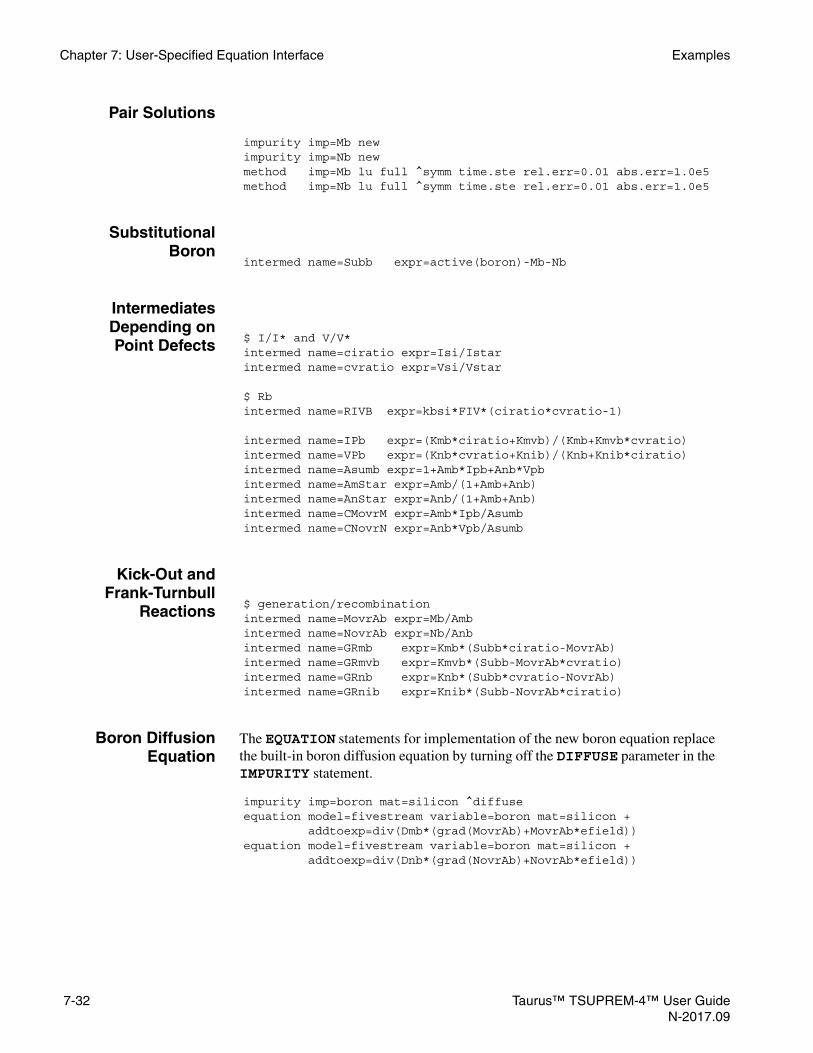
Chapter 7: User-Specified Equation Interface Examples

Pair Solutions

SubstitutionalBoron

IntermediatesDepending onPoint Defects

Kick-Out andFrank-Turnbull

Reactions

Boron DiffusionEquation

The EQUATION statements for implementation of the new boron equation replace the built-in boron diffusion equation by turning off the DIFFUSE parameter in the IMPURITY statement.

impurity imp=Mb newimpurity imp=Nb newmethod imp=Mb lu full ^symm time.ste rel.err=0.01 abs.err=1.0e5method imp=Nb lu full ^symm time.ste rel.err=0.01 abs.err=1.0e5

intermed name=Subb expr=active(boron)-Mb-Nb

$ I/I* and V/V*intermed name=ciratio expr=Isi/Istarintermed name=cvratio expr=Vsi/Vstar

$ Rbintermed name=RIVB expr=kbsi*FIV*(ciratio*cvratio-1)

intermed name=IPb expr=(Kmb*ciratio+Kmvb)/(Kmb+Kmvb*cvratio)intermed name=VPb expr=(Knb*cvratio+Knib)/(Knb+Knib*ciratio)intermed name=Asumb expr=1+Amb*Ipb+Anb*Vpbintermed name=AmStar expr=Amb/(1+Amb+Anb)intermed name=AnStar expr=Anb/(1+Amb+Anb)intermed name=CMovrM expr=Amb*Ipb/Asumbintermed name=CNovrN expr=Anb*Vpb/Asumb

$ generation/recombinationintermed name=MovrAb expr=Mb/Ambintermed name=NovrAb expr=Nb/Anbintermed name=GRmb expr=Kmb*(Subb*ciratio-MovrAb)intermed name=GRmvb expr=Kmvb*(Subb-MovrAb*cvratio)intermed name=GRnb expr=Knb*(Subb*cvratio-NovrAb)intermed name=GRnib expr=Knib*(Subb-NovrAb*ciratio)

impurity imp=boron mat=silicon ^diffuseequation model=fivestream variable=boron mat=silicon +

addtoexp=div(Dmb*(grad(MovrAb)+MovrAb*efield))equation model=fivestream variable=boron mat=silicon +

addtoexp=div(Dnb*(grad(NovrAb)+NovrAb*efield))

7-32 Taurus™ TSUPREM-4™ User GuideN-2017.09

Examples Chapter 7: User-Specified Equation Interface

Pair DiffusionEquations

For the boundary condition, the dopant-defect pairs are annihilated at interfaces by turning off TRANSPORT, since the dopant-defect pairs exist only in silicon.

Point DefectEquations

The interstitial and vacancy variables are the free interstitial and vacancy concentrations, respectively. In the 3-stream diffusion models, PD.TRANS or PD.FULL, the dopant-defect pairs are instantly determined before the first post-implant anneal, so that the total point-defect concentrations are conserved by subtracting the dopant-defect pairs and the interstitial small clusters from the total concentrations. When the interstitial or vacancy solution variables are used, they are the free not total concentrations. However, the interstitial or vacancy variables used in the INITIAL parameter are the total concentrations.

The surface recombination is described as follows:

Since the initialization uses the built-in calculation of the point defects for implantation, Isi and Vsi in the structure must be added to the generated built-in point defects due to implantation. After initializing and adding Isi and Vsi, the built-in point defect solutions are eliminated by setting PD.FERMI.

equation model=fivestream variable=Mb mat=silicon + initial="exist(Mb)?Mb:1E5" + addtoexp=div(Dmb*(grad(MovrAb)+MovrAb*efield))+GRmb+GRmvbequation model=fivestream variable=Nb mat=silicon + initial="exist(Nb)?Nb:1E5" + addtoexp=div(Dnb*(grad(NovrAb)+NovrAb*efield))+GRnb+GRnib

$ equilibrium M* and N*intermed name=MbStar expr=AmStar*eqact(boron,boron)intermed name=NbStar expr=AnStar*eqact(boron,boron)$ boundary equationsequation model=fivestream variable=Mb mat1=silicon /mat2=oxide + ^transpor interfac=-Trans*(onmat1(Mb/Seg-MbStar))equation model=fivestream variable=Nb mat1=silicon /mat2=oxide + ^transpor interfac=-Trans*(onmat1(Nb/Seg-NbStar))

equation model=fivestream variable=Isi mat=silicon + initial=”damage>1.15e22? IStar: +

(exist(Isi)?interstitial+Isi:interstitial)” + addtoexp=div(DI*IStar*grad(ciratio))-RIVB-GRmb+GRnibequation model=fivestream variable=Vsi mat=silicon + initial=”damage>1.15e22?VStar: +

(exist(Vsi)?vacancy+Vsi:vacancy)” + addtoexp=div(DV*VStar*grad(cvratio))-RIVB-GRnb+GRmvb

equation model=fivestream variable=Isi mat=silicon /mat=oxide + interfac=-ksurfi*onmat1(Isi-IStar) ^transporequation model=fivestream variable=Vsi mat=silicon /mat=oxide + interfac=-ksurfv*onmat1(Vsi-VStar) ^transpor

Taurus™ TSUPREM-4™ User Guide 7-33N-2017.09

Chapter 7: User-Specified Equation Interface Examples

For example:

Coupling With Small Clusters

To see the certain effect of the 5-stream diffusion model, the non-equilibrium status for the formation of dopant-defect pairs must be dominant in the diffusion process. The diffusion process is usually performed at very low temperature and/or for very short time. The small clusters must be taken into account for such a process condition. In TSUPREM-4, the small clusters, I2 and BI2, are assumed to form competitively with the boron-interstitial pair formation by assuming that I2, BI2 and Mb(boron-interstitial pair) are in equilibrium. Thus, the initialization of the small clusters with the zero dopant-defect pair concentrations is not physical. Unless the transient equations are implemented for I2 and BI2 formation in non-equilibrium, it is not possible to account for the small clusters in the 5-stream diffusion model. It will be shown how the initialized profiles of I2, BI2, I(free interstitial), and Mb in the built-in codes are different from those in the 5-stream model using USEIT.

Interstitial SmallClusters - I2

method model=fivestream enable$ turn on PD.TRANS in order to use the built-in initializationmethod pd.transimplant boron dose=1e14 energy=20

$ initialize Isi and Vsidiffuse temp=900 time=0

$ remove the built-in point defect solutionsmethod pd.fermi

diffuse temp=900 time=10/60

$ reinitialize Isi and Vsi for the second implantmethod pd.transimplant boron dose=1e15 energy=10diffuse temp=1000 time=0method pd.fermi

diffuse temp=1000 time=5/60

$ reaction for I small clustersloop steps=5 index=i start=-2 intermed name=kI[@i] expr=kI0[@i]*exp(-(kIE[@i])/kt)l.end$ I small clustersintermed name=Fcv + expr=ciratio*ViStar*sum(i,-2,2, +

sum(j,-2,2,kcV[i][j]*kI[i]*phiV[j]*ETA^(-i-j)))intermed name=Ic expr=2*ciratio^2*sum(i,-2,2,kI[i]/ETA^i)intermed name=rc expr=RIVB/IiStar/ViStar*Fcvequation model=fivestream var=Isi mat=si addtoexp=-ddt(Ic)-rcequation model=fivestream var=Vsi mat=si addtoexp=-rc

7-34 Taurus™ TSUPREM-4™ User GuideN-2017.09

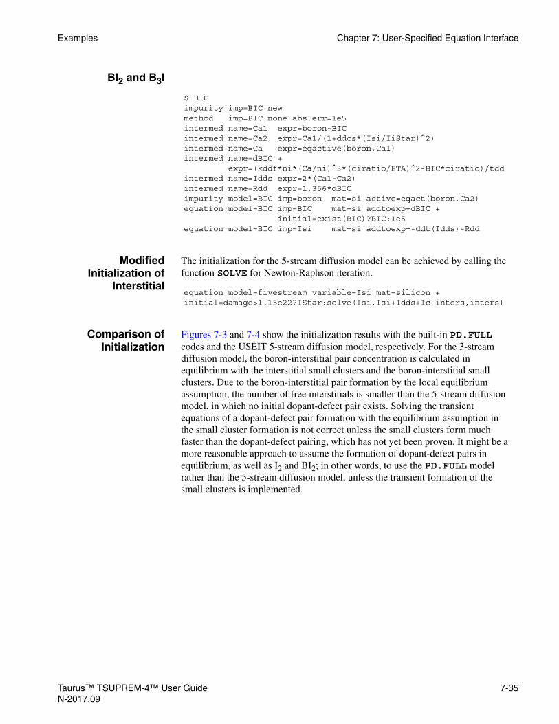
Examples Chapter 7: User-Specified Equation Interface

BI2 and B3I

ModifiedInitialization of

Interstitial

The initialization for the 5-stream diffusion model can be achieved by calling the function SOLVE for Newton-Raphson iteration.

Comparison ofInitialization

Figures 7-3 and 7-4 show the initialization results with the built-in PD.FULL codes and the USEIT 5-stream diffusion model, respectively. For the 3-stream diffusion model, the boron-interstitial pair concentration is calculated in equilibrium with the interstitial small clusters and the boron-interstitial small clusters. Due to the boron-interstitial pair formation by the local equilibrium assumption, the number of free interstitials is smaller than the 5-stream diffusion model, in which no initial dopant-defect pair exists. Solving the transient equations of a dopant-defect pair formation with the equilibrium assumption in the small cluster formation is not correct unless the small clusters form much faster than the dopant-defect pairing, which has not yet been proven. It might be a more reasonable approach to assume the formation of dopant-defect pairs in equilibrium, as well as I2 and BI2; in other words, to use the PD.FULL model rather than the 5-stream diffusion model, unless the transient formation of the small clusters is implemented.

$ BICimpurity imp=BIC newmethod imp=BIC none abs.err=1e5intermed name=Ca1 expr=boron-BICintermed name=Ca2 expr=Ca1/(1+ddcs*(Isi/IiStar)^2)intermed name=Ca expr=eqactive(boron,Ca1)intermed name=dBIC + expr=(kddf*ni*(Ca/ni)^3*(ciratio/ETA)^2-BIC*ciratio)/tddintermed name=Idds expr=2*(Ca1-Ca2)intermed name=Rdd expr=1.356*dBICimpurity model=BIC imp=boron mat=si active=eqact(boron,Ca2)equation model=BIC imp=BIC mat=si addtoexp=dBIC +

initial=exist(BIC)?BIC:1e5equation model=BIC imp=Isi mat=si addtoexp=-ddt(Idds)-Rdd

equation model=fivestream variable=Isi mat=silicon +initial=damage>1.15e22?IStar:solve(Isi,Isi+Idds+Ic-inters,inters)

Taurus™ TSUPREM-4™ User Guide 7-35N-2017.09

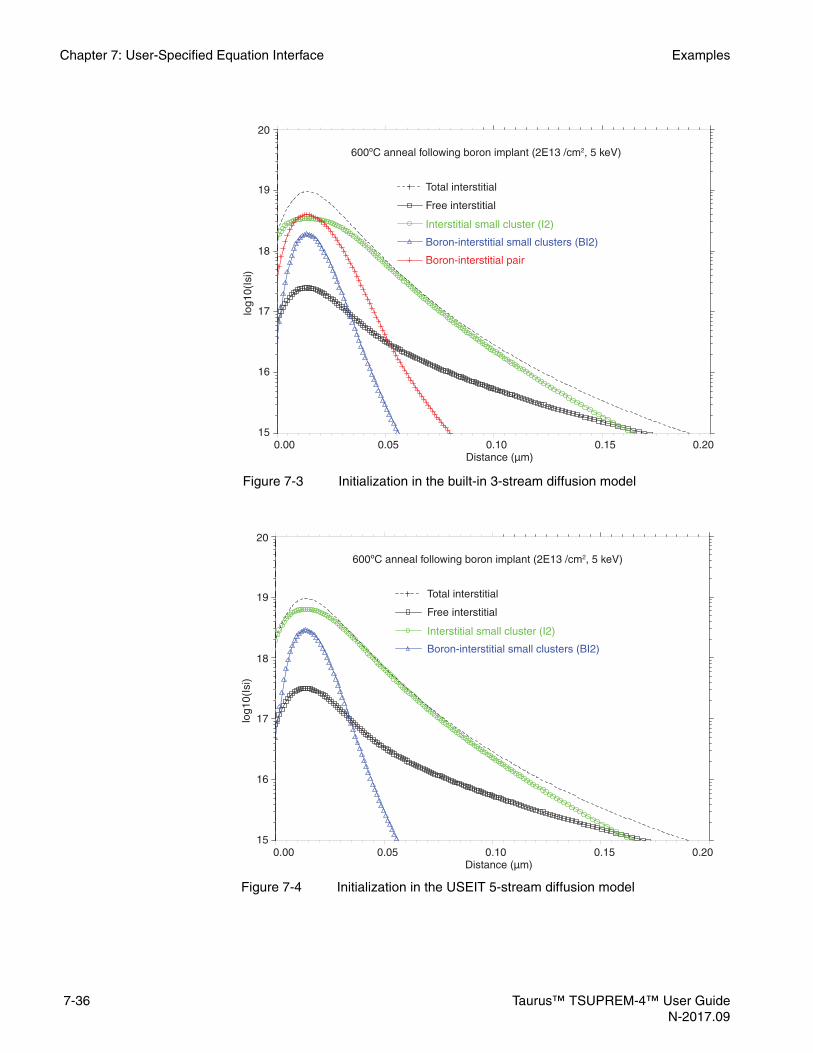
Chapter 7: User-Specified Equation Interface Examples

20

19

18

17

16

150.00 0.05 0.10 0.15 0.20

Distance (µm)

log1

0(Is

i)

600ºC anneal following boron implant (2E13 /cm2, 5 keV)

Total interstitial

Free interstitial

Interstitial small cluster (I2)

Boron-interstitial small clusters (BI2)

Boron-interstitial pair

Figure 7-3 Initialization in the built-in 3-stream diffusion model

20

19

18

17

16

150.00 0.05 0.10 0.15 0.20

Distance (µm)

log1

0(Is

i)

600ºC anneal following boron implant (2E13 /cm2, 5 keV)

Total interstitial

Free interstitial

Interstitial small cluster (I2)

Boron-interstitial small clusters (BI2)

Figure 7-4 Initialization in the USEIT 5-stream diffusion model

7-36 Taurus™ TSUPREM-4™ User GuideN-2017.09

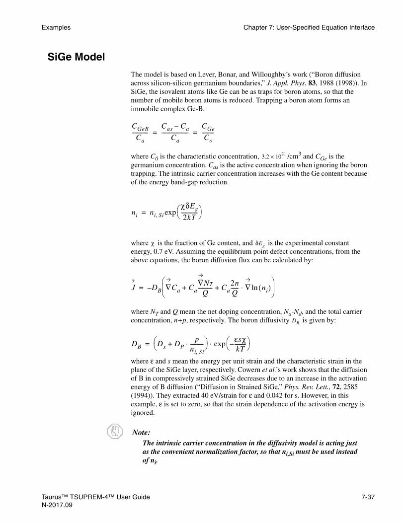
Examples Chapter 7: User-Specified Equation Interface

SiGe Model

The model is based on Lever, Bonar, and Willoughby’s work (“Boron diffusion across silicon-silicon germanium boundaries,” J. Appl. Phys. 83, 1988 (1998)). In SiGe, the isovalent atoms like Ge can be as traps for boron atoms, so that the number of mobile boron atoms is reduced. Trapping a boron atom forms an immobile complex Ge-B.

where C0 is the characteristic concentration, /cm3 and CGe is the germanium concentration. Cas is the active concentration when ignoring the boron trapping. The intrinsic carrier concentration increases with the Ge content because of the energy band-gap reduction.

where is the fraction of Ge content, and is the experimental constant energy, 0.7 eV. Assuming the equilibrium point defect concentrations, from the above equations, the boron diffusion flux can be calculated by:

where NT and Q mean the net doping concentration, Na-Nd, and the total carrier concentration, n+p, respectively. The boron diffusivity is given by:

where ε and s mean the energy per unit strain and the characteristic strain in the plane of the SiGe layer, respectively. Cowern et al.’s work shows that the diffusion of B in compressively strained SiGe decreases due to an increase in the activation energy of B diffusion (“Diffusion in Strained SiGe,” Phys. Rev. Lett., 72, 2585 (1994)). They extracted 40 eV/strain for ε and 0.042 for s. However, in this example, ε is set to zero, so that the strain dependence of the activation energy is ignored.

Note:The intrinsic carrier concentration in the diffusivity model is acting just as the convenient normalization factor, so that ni,Si must be used instead of ni.

CGeB

Ca------------

Cas Ca–

Ca--------------------

CGe

Co---------= =

3.2 1021×

ni ni Si,χδEg

2kT------------- exp=

χ δEg

J DB ∇Ca Ca∇NT

Q----------- Ca

2nQ------ ∇ ni( )ln⋅+ +

–=

DB

DB Dx DPp

ni Si,----------⋅+

εsχkT--------–

exp⋅=

Taurus™ TSUPREM-4™ User Guide 7-37N-2017.09

Chapter 7: User-Specified Equation Interface Examples

impurity imp=Germanium new

intermed name=GeMax express=5e22intermed name=StrainMax express=0.042intermed name=GeFrac express=Germanium/GeMaxintermed name=StrainSiGe express=GeFrac*StrainMax

intermed name=EaStrain express=0 ;$ instead of 40intermed name=dEa express=EaStrain*StrainSiGeintermed name=DX0 expr=0.0368intermed name=DBE expr=3.46+dEaintermed name=DP0 expr=0.716intermed name=Db size=2 minindex=0 +

expr="DX0*exp(-DBE/kt),DP0*exp(-DBE/kt)"

intermed name=dEg express=0.7intermed name=Ni expr=3.87e16*exp(-0.605/kt+1.5*log(temp))intermed name=NiSiGe express=Ni*exp(GeFrac*dEg/(2*kt))intermed name=C0 express=3.2e21intermed name=fTrap express=1/(1.0+Germanium/C0)

intermed name=Na express=active(boron)intermed name=Nd express=active(arsenic)+active(phosphorus)intermed name=Nt express=fTrap*(Na-Nd)intermed name=Q express=sqrt(Nt^2+4*NiSiGe^2)intermed name=nelectron express=0.5*(Q-Nt)intermed name=nhole express=0.5*(Q+Nt)intermed name=DbSiGe express=Db[0]+Db[1]*nhole/Niintermed name=Bmobile express=fTrap*active(boron)

equation model=sige variable=boron mat=si +addtoexp=”div(DbSiGe*(grad(Bmobile)+ +Bmobile/Q*(grad(Nt)+2*nelectron*grad(log(NiSiGe)))))”

impurity imp=boron mat=si ^diffuse

7-38 Taurus™ TSUPREM-4™ User GuideN-2017.09

CHAPTER 8

TN

Advanced Calibration8

This chapter describes the use of the TSUPREM-4 Advanced Calibration file with the Merger application.

OverviewThe TSUPREM-4 Advanced Calibration file helps to obtain accurate results with TSUPREM-4. The choice of physical models is widely based on the Advanced Calibration of Sentaurus Process [1] and is calibrated with the help of a SIMS database.

In 2006, a complete recalibration of TSUPREM-4 models was performed. Parameters obtained during that work are collected in the s4advanced.2008.09 file. The parameters of boron segregation at silicon/oxide interfaces have been updated in s4advanced.2013.12. Besides boron segregation, s4advanced.2008.09 and s4advanced.2013.12 are identical. They provide a significant improvement of simulation results in comparison to earlier file versions. You can invoke the new set of models and parameters by typing one line in any place in the input file:

method advanced

Simulation results obtained with this command are very accurate. For further result improvements, you can use the initial conditions after an implantation step, depending on the energy or dose. A special Merger application file [1] contains a definition of an energy and dose-dependent initial dopant activation level.

Parameter File

Advanced Calibration is a selection of physical models and model parameters, which are recommended by Synopsys to be used for accurate process simulation. In TSUPREM-4, this selection of models and parameters is contained in a parameter file named s4advanced.2013.12 which is located in the TSUPREM-4

aurus™ TSUPREM-4™ User Guide 8-1-2017.09

Chapter 8: Advanced Calibration Overview

library (s4lib directory). The following section describes the contents of that file.

The s4advanced.2013.12 models and parameters are invoked inside the Merger file named AdvCal_1d_tables_2008.09.smr. The file can be merged with a TSUPREM-4 input file, which contains only the pure process flow without any choice of physical models and parameters, using the Merger application. This is described below.

Note:The Merger application is part of Sentaurus Workbench Advanced. Merger tests if the corresponding license (swb-advanced) exists at the user site, but does not block the license.

For additional calibration, you can copy the Merger file to a local directory and edit with any standard text editor. The following section details contents of that file.

Merging a Process Flow and Parameter File With Merger

Three types of information are needed to perform a process simulation:

• The device fabrication process to be simulated which includes the substrate doping and all implantation, diffusion, oxidation, deposition, and etching steps.

• The physical models and model parameters to be used in the process simulation.

• The mesh for the process simulation.

With the Merger application the information about the fabrication process and the physical models and parameters can be separated into two different files:

• The Merger file contains the process flow.

• The TSUPREM-4 Rules file contains the choice of physical models and parameters.

The commands for creating and refining the mesh are part of either the Merger file or the TSUPREM-4 Rules file. Merger inserts the information contained in the TSUPREM-4 Rules file correctly into the process flow and, thereby, creates a complete TSUPREM-4 input file.

The separation of the process flow and the choice of physical models and parameters has the following advantages:

• The Merger file, which contains only the process flow, is easy to read and edit, even for non-TCAD experts.

• It is easy to ensure that the same process simulation models are applied to 1D simulation tasks (SIMS data calibration) and 2D simulation tasks (full process and device simulation).

8-2 Taurus™ TSUPREM-4™ User GuideN-2017.09

Overview Chapter 8: Advanced Calibration

• All calibration work is contained in the TSUPREM-4 Rules file. A single rules file can be applied to different process flows which makes it easier to transfer calibration results to another technology node.

TSUPREM-4 Rules File

AdvCal_1d_tables_2008.09.smr is used as a TSUPREM-4 Rules file by Merger. For additional calibration, you can make a local copy of the TSUPREM-4 Rules file and edit it with a text editor or with the graphical user interface (GUI) of Merger [1].

The TSUPREM-4 Rules file consists of five sections. The first two are brief and specify the process simulator and the title of the Rules file, for example:

Simulator { TSUPREM-4 }

Title {1D TSUPREM-4 A-2008.09}

The other three sections are a gridblock, a startblock, and a list of pattern-actions.

The gridblock has the format:

Gridblock {...

}

The initial 1D simulation mesh and the criteria for mesh refinement are in AdvCal_1d_tables_2008.09.smr. The default 1D simulation mesh is fine enough for process simulation ranging from ultrashallow junction formation to power technologies.

In 2D application projects, the gridblock must contain the mesh specification and adaptation parameters for the 2D simulation. Alternatively, since the ideal 2D mesh strongly depends on the device geometry and size, you can consider removing all commands from the gridblock. If the gridblock is empty, you must provide the information about the initial grid and mesh refinement in the Merger file, which contains the process flow.

Taurus™ TSUPREM-4™ User Guide 8-3N-2017.09

Chapter 8: Advanced Calibration Overview

The startblock is very short:

Startblock {method advanced

$ C-I clustering model$=====================$ To use C-I clustering model, remove "$" from 2 lines below.$ method ddc.full$ method precond=2

$ 5-stream diffusion model$ ========================$ To use the 5-stream model, remove "$" from the line below.$ method nstreams=5

$ Complex models$ ========================$ To use complex models, remove "$" from line below.$ source s4advanced_complex.2008.09}

TSUPREM-4 models and parameters contained in s4advanced.2008.09 are invoked by the first line. They will be used as the default for the whole process simulation. The rest of the block consists of three sections by which you can select the:

• Carbon–interstitial clustering model

• Five-stream diffusion model

• Set of the advanced interstitial clustering and dopant activation models.

Note:You must remove $ from the beginning of the corresponding lines. When merging the Merger file with the TSUPREM-4 Rules file, the gridblock and startblock are inserted at the beginning of the complete TSUPREM-4 input file.

Some physical parameters depend on special process steps. For example, the amount of damage created by an ion implantation depends on the details of the implantation. For such physical parameters, it is impossible to fix their values once at the beginning for the whole process simulation. Instead, the values must be set where needed. For example, the initial activation of boron atoms after boron implantation must be set for each boron implantation individually, depending on the implantation energy and dose. All these process step–related parameters are contained in the last part of the TSUPREM-4 Rules file, that is, the list of pattern-actions.

A typical pattern-action of a TSUPREM-4 Rules file is:

Condition (1) if ( implantation && element==indium {prepend impurity impurity=indium mat=silicon +act.ni=0.0 c1frac.a=1.0 +act.amor=5.e20 c1.ini.f=0.3 ddctot.c=0.3}

}

8-4 Taurus™ TSUPREM-4™ User GuideN-2017.09

Overview Chapter 8: Advanced Calibration

With this pattern-action in the TSUPREM-4 Rules file, Merger will evaluate it for all implantation statements of the process flow if the element is indium. For each implantation statement where this is the case (that is, where the ‘pattern’ is found), Merger will insert:

impurity impurity=indium mat=silicon act.ni=0.0 c1frac.a=1.0 + act.amor=5.e20 c1.ini.f=0.3 ddctot.c=0.3

before the implant line of the TSUPREM-4 input file. This will set the initial activation level to in the amorphized region and the indium cluster fraction to 0.3 in the crystalline region. A detailed reference to the syntax of pattern-actions is given in the Advanced Calibration for Process Simulation User Guide [1].

Merging a MergerFile and

TSUPREM-4Rules File

The Merger application is used to merge the Merger file and the Rules file to a complete TSUPREM-4 input file. This can be performed interactively or in batch mode. The interactive mode is started by typing:

merger

A graphical user interface (GUI) opens, the Merger file and TSUPREM-4 Rules file can be loaded, and the merging can be performed [1].

In batch mode, without starting the GUI, Merger can be started from the command line, for example:

merger -batch -process process_flow.txt -rules AdvCal_1d_tables_2008.09.smr -output full_ts4.cmd

This line merges the Merger file process_flow.txt and the Rules file AdvCal_1d_tables_2008.09.smr, and creates the complete TSUPREM-4 input file full_ts4.cmd.

In Sentaurus Workbench projects, it is convenient to execute Merger in batch mode, without starting the GUI. This lets you insert the physical models and parameters to process flow files for many different split conditions. A single TSUPREM-4 Rules file is merged with many Merger files, each representing one of the process split conditions, which were previously preprocessed by Sentaurus Workbench.

Reference [1] describes how to configure the TSUPREM-4 prologue of Sentaurus Workbench for an automatic merging of preprocessed process flow files.

Monte Carlo Implantation

By default, analytic implantation is used with AdvCal_1d_tables_2008.09.smr. To use Monte Carlo implantation instead, switch on the pattern-action:

Condition (0) if (implantation) {insert {montecarlo n.ion=5000 dose.spl traj.spl}

}

5.0 1020× cm

3–

Taurus™ TSUPREM-4™ User Guide 8-5N-2017.09

Chapter 8: Advanced Calibration Models and Parameters

by replacing Condition (0) with Condition (1)

To use Monte Carlo implantation only for selected dopants, add a pattern-action, which inserts the keyword montecarlo only into the selected implants. For example, the following pattern-action switches on Monte Carlo implantation only for boron implants:

Condition (1) if (implantation && element==Boron) {insert {montecarlo n.ion=5000 dose.spl traj.spl}

}

Models and ParametersThe choice of models is almost the same as in the Advanced Calibration of Sentaurus Process [1]. Where possible, the options of the diffusion models are selected in such a way that the same equations are solved in Sentaurus Process and TSUPREM-4.

However, due to some differences in the implementation of physical models in TSUPREM-4 and Sentaurus Process, some parameters differ from the corresponding parameters in the Advanced Calibration of Sentaurus Process, to give optimal results with TSUPREM-4. These adjustments are based on a calibration using SIMS data.

All model switches and parameters that are not set in the calibration file have the TSUPREM-4 default values.

Models of Advanced Calibration of TSUPREM-4

The Advanced Calibration of TSUPREM-4 is based on the following selection of implantation and diffusion models:

• Analytic tables for all implantations. Alternatively, Monte Carlo implantation can be used.

• Pair diffusion framework (method pd.full). In silicon, the diffusing species are point defects (interstitials and vacancies) and pairs of a dopant and a point defect. As an option, the five-stream model can be used. In the five-stream model, the concentration of dopant–defect pairs is not in local equilibrium with substitutional dopants and free point defects.

• The +N-model for the initial interstitial concentration after ion implantation.

• The one-moment clustering model for interstitials.

• First-order reaction equations for clusters of dopant impurities. There is only one reaction equation per impurity, which governs the relationship between active and total concentrations.

• Dopant segregation at interfaces. Dose loss is described by the three-phase segregation model for all dopants.

8-6 Taurus™ TSUPREM-4™ User GuideN-2017.09

Models and Parameters Chapter 8: Advanced Calibration

• The model for Ge chemical and strain effects.

• The carbon–interstitial clustering model.

Contents of AdvCal_1d_tables_2008.09.smr

Gridblock The gridblock is inserted at the beginning of a TSUPREM-4 input file. The gridblock contents of AdvCal_1d_tables_2008.09.smr is intended to create a good 1D mesh.

A 1D mesh is prepared with a fine resolution near the silicon surface and with a coarser grid spacing in the deeper regions of the simulation. Mesh adaptation is switched off for implantation and diffusion. Mesh adaptation can be helpful in reducing CPU time by having a good mesh refinement only in specified regions. However, for 1D simulations, CPU time is often not an issue because the simulations are very fast.

This 1D mesh is fine enough for almost all 1D investigations, with one exception– If the diffusion of thin dopant marker layers is investigated, it is necessary to create a fine mesh in the neighborhood of the marker layers, which can be located far away from the silicon surface.

For 2D applications, the gridblock needs to be edited in one of the following ways:

• You can enter correct specifications for 2D mesh generation into the gridblock.

• You can work with an empty gridblock and place the specifications for 2D mesh generation directly into the TSUPREM-4 Merger file, which contains the process flow.

Startblock The startblock is inserted at the beginning of a TSUPREM-4 input file, immediately after the gridblock. By default, it contains only one line:

method advanced

This command is used to invoke models and parameters defined in s4advanced.2013.12. The file contents are described below.

Basic ModelSelection

The Taurus implantation tables are used for all important implantation species:

impurity impurity=arsenic impl.tab=taurusimpurity impurity=antimony impl.tab=taurusimpurity impurity=boron impl.tab=taurusimpurity impurity=indium impl.tab=taurusimpurity impurity=phosphorus impl.tab=taurusimpurity impurity=germanium impl.tab=taurusimpurity impurity=fluorine impl.tab=taurusimpurity impurity=nitrogen impl.tab=taurusimpurity impurity=carbon impl.tab=taurus

Ge, C, F, and N implantations are simulated by the newly created tables.

Taurus™ TSUPREM-4™ User Guide 8-7N-2017.09

Chapter 8: Advanced Calibration Models and Parameters

For diffusion, the basic selection is:

method pd.full ^pair.rec ^pd.prec

With this line, the three-stream diffusion model is selected (pd.full), and the dopant-assisted recombination of interstitials and vacancies is switched off (^pair.rec ^pd.prec).

+N - Model +N-model is used to calculate the amount of excess interstitial generated by ion implantation. A new TSUPREM-4 feature lets you define +N-model factors dependent on the implant energy and dose. Corresponding statements can be found in s4advanced.2013.12. For example:

impurity imp=arsenic d.plus="(${E}+1.0)/(${E}+3.0)"

The above command is invoked to decrease the arsenic d.plus for low implant energies. The advantage of such an approach is that you can avoid the definition of the energy dependent factors in the Rules file.

If d.plus is not specified explicitly, the default value equal to 1.0 is used. It is defined by the following line:

material mat=silicon d.phdf=0.0 d.pconst=0.0

Intrinsic CarrierConcentration

The intrinsic carrier concentration is modified to give a good fit in the temperature range between and to the formula suggested by Morin and Maita [2]:

material silicon ni.0=8.23e16 ni.e=0.656 ni.f=1.5

Point-DefectModels andParameters

• Bulk silicon:

For interstitials and vacancies, the same diffusivity, equilibrium concentration, charge-state distribution, and bulk recombination are used as in the Advanced Calibration of Sentaurus Process [1].

• Surface boundary conditions:

The v.norm recombination model was chosen for the Si–SiO2 interface. The recombination velocity is specified, for interstitials, by the parameters:

ksurf.0=1.78e8 ksurf.e=1.73

and, for vacancies, by the parameters:

ksurf.0=1.42e5 ksurf.e=1.75

With these parameters, the interface acts as an efficient sink for point defects generated by an implantation. The influence of oxide growth on point defect recombination is switched off (ksvel.0=0, ksvel.e=0).

The default growth model is used to simulate the injection of interstitials during silicon oxidation. The model parameters were extracted from oxidation-enhanced diffusion (OED) experiments:

theta.e0=7.3e4 theta.e=2.1 gpow.0=-0.4 gpow.e=0.0

700°C 1100°C

8-8 Taurus™ TSUPREM-4™ User GuideN-2017.09

Models and Parameters Chapter 8: Advanced Calibration

• Interstitial clusters:

The 1Moment model is used for interstitial clusters with similar parameters as in the Sentaurus Process calibration. The calibration is based on TEM data on the dissolution of {311} defects during thermal anneal, published in the literature [3][4]. The shrinking of interstitial clusters by recombination with vacancies is switched off for the benefit of consistency with the Sentaurus Process calibration.

Small clusters of interstitials and vacancies are not included in the simulation (eclust.n=0).

Dopant Modelsand Parameters

The same basic model set is used for all dopants and includes the following:

• Three-stream or five-stream diffusion model depending on user selection

• Transient dopant clustering model

• Three-phase segregation model

• Model for Ge chemical and stress effects

These models are described here. Dopant-specific model features are explained after the common model description.

• Dopant diffusion:

The three-stream pair diffusion model is chosen by default. In this model, dopant–defect pairs are in local equilibrium with substitutional dopants and free point defects. The diffusivities of boron, arsenic, indium, and antimony have the same values as in the Advanced Calibration of Sentaurus Process. The microscopic diffusivity of dopant–defect pairs is set equal to the diffusivity of point defects. The recombination between dopant–defect pairs and free defects is switched off by setting the reaction radii r.ip.v and r.vp.i to 0. Ion pairing is switched on for all dopants by using:

material material=silicon ion.pair

Alternatively, you can use the five-stream pair diffusion model. In this case, users must add the following line to the input file:

method nstreams=5

or uncomment the corresponding line in AdvCal_1d_tables_2008.09.smr.

Furthermore, the parameters r.i.s, e.i.s, r.v.s, and e.v.s, which define the rates of formation and dissolution of dopant–defect pairs, are specified for all dopants. Their values have been obtained by translation of Sentaurus Process Advanced Calibration parameters.

• Dopant clusters:

To use transient formation and dissolution of dopant clusters, use the following line:

method act.full

With this command, TSUPREM-4 switches on five models for dopant activation in parallel: a solid solubility model, an equilibrium dopant

Taurus™ TSUPREM-4™ User Guide 8-9N-2017.09

Chapter 8: Advanced Calibration Models and Parameters

clustering model, an equilibrium dopant–defect clustering model, a precipitation model, and a transient dopant–defect clustering model.

Clusters are assumed to be neutral.

In the Advanced Calibration, only the transient dopant–defect clustering model is used, and the other models are switched off by an appropriate choice of parameters. Furthermore, it is assumed that no interstitials take part in the formation and dissolution of clusters (ddcf.i.n=0 ddcr.i=0 ifracm=0). The parameters used for the calibration of the transient dopant–defect clustering model are:

• ddc.f.0, ddc.f.e: Define the equilibrium between clusters and substitutional dopants.

• ddc.t.0, ddc.t.e: Adjust the reaction time needed to approach equilibrium.

The parameters ddcf.d.n, ddcf.n.n, and ddcr.n.n are specified in such a way that the same number of dopants and electrons take part in the cluster formation and dissolution as in the Advanced Calibration of Sentaurus Process.

As previously mentioned, the other activation reactions that are offered by method act.full are switched off. This reduces the power of the model to capture several physical phenomena in parallel. On the other hand, the complexity is reduced and the calibration is more reliable for most applications. Switching off the other activation models is performed in the same way for all dopants. For example, in the case of arsenic, it is performed with the following commands and parameters:

• The solid solubility model is switched off by setting the solid solubility to a very high level:

impurity imp=arsenic mat=si ss.clear

impurity imp=arsenic mat=si ss.temp=450 ss.conc=1.0e23

impurity imp=arsenic mat=si ss.temp=1500 ss.conc=1.0e23

• The equilibrium dopant clustering model is switched off with the following parameters:

impurity mater=silicon imp=arsenic ctn.0=0.0 ctn.e=0.0

• The precipitation model is switched off by using:

impurity mater=silicon imp=arsenic c0.tf.0=0.0 + c0.tf.e=0.0 c0.tr.0=0.0 c0.tr.e=0.0

Indium is not a built-in dopant of TSUPREM-4; therefore, indium clusters must be defined by additional lines that are not needed for the other main dopants:

impurity imp=c1_indium new c.init=1e5

impurity imp=indium imp.cl1=c1_indium

method imp=c1_indium lu none ̂ symm time.ste rel.err=0.01 +abs.err=1.0e9 temp.min=450

8-10 Taurus™ TSUPREM-4™ User GuideN-2017.09

Models and Parameters Chapter 8: Advanced Calibration

Initial conditions independent of implantation conditions are defined in s4advanced.2008.09:

impurity impurity=arsenic mat=silicon act.ni=0.0 +

c1frac.a=1.0 act.amor=2.0e20 c1.ini.f=0.7 + ddctot.a=1.0 ddctot.c=0.7

Two last parameters (ddctot.a, ddctot.c) are necessary when the full dynamics dopant–defect clustering model (method ddc.full) is switched on to simulate a formation of carbon–interstitial clusters.

Note:dctot.c must be equal to c1.ini.f.

• Three-phase segregation model:

For all dopants, the dose loss at the Si–SiO2 interface is simulated by the three-phase segregation model. It is assumed that the trapped dopant is in the neutral charge state. The charge state is defined by the number of carriers annihilated during trapping. For example, if one electron is annihilated during arsenic trapping, then the trapped atom will be neutral:

impurity impurity=arsenic mat=silicon /mat=oxide + seg.cpow=1.0

The parameters of the three-phase segregation model were calibrated using the internal SIMS database. The diffusivity of dopants along the Si–SiO2 interface is set to zero.

When using the five-stream framework, the pair segregation model is invoked:

method pair.seg

According to this model, a dissociation of dopant–defect pairs occurs at the Si–SiO2 interface. Such an approach looks more reasonable than an assumption about pair recombination used in the default model. The parameters seg.ipow and seg.vpow are set to zero for the consistency with simulation results obtained by using the three-stream diffusion model.

Note:Current boron segregation parameters may give inaccurate results in the case of the fast oxidation at high temperatures. An additional calibration may be needed for such process conditions.

• Stress and germanium chemical effects:

The TSUPREM-4 pressure-dependent diffusion model with default activation volumes is used in the Advanced Calibration to simulate the stress effect:

method st.diff

In addition, the energy bandgap dependence on the pressure and local Ge content is considered:

method gapsige enable

Taurus™ TSUPREM-4™ User Guide 8-11N-2017.09

Chapter 8: Advanced Calibration Models and Parameters

The Ge chemical effect is modeled in several ways:

• First, the energy band gap changes as previously mentioned.

• Second, dopant diffusivity dependence on the local Ge concentration is introduced. The interstitial and vacancy components change separately as shown below for phosphorus:

impurity imp=phosphorus mat=si +di.fac=exp(1.2e-23*germanium/kT)

impurity imp=phosphorus mat=si +dv.fac=exp(2.2e-23*germanium/kT)

• Third, a simple TSUPREM-4 model is invoked to simulate the reduction of the active boron concentration due to Ge–B pair formation:

method geandb enable

Stress and Ge chemical effect models are different from ones used in the Advanced Calibration of Sentaurus Process. They have been transferred from s4advanced.2006.06.

• High concentration arsenic and antimony diffusion:

At high donor concentrations, the diffusivity of As–V pairs is increased, following the ideas of Dunham and Wu [5], and based on experimental data from Larsen et al. [6]. This is achieved by using:

impurity imp=arsenic mater=silicon +dv.fac=(2.3e-23*germanium/kT)* +

(1.0+((active(arsenic)+(active(phosphorus))/ +1.9e20)^3.5)

Similarly, the diffusivity of Sb–V pairs is increased in regions of high Sb doping:

impurity imp=antimony mater=silicon +dv.fac=(1.7e-23*germanium/kT)* +

(1.0+((active(antimony))/2.0e20)^3.5)

• Indium dose loss:

The limitation of the indium concentration in amorphized regions is switched on by the line:

impurity mat=silicon imp=indium max.amor=6.e18

The reason for the dose loss is that indium atoms are swept out of silicon during the regrowth of the amorphous layer due to the segregation at the amorphous–crystalline interface [7].

• Boron diffusivity in oxide:

The boron diffusivity in oxide is increased for highly doped oxides by defining the multiplication factor di.fac:

impurity mat=oxide imp=boron di.fac=(1.0+fluorine/ +2.0e18+bddl/(bdi*(1.0+(1.e21/ +(arsenic+boron+phosphorus+indium + antimony+germanium+1.e5))^2))* +(1+(boron/6.0e20)*(boron/6.0e20)))

8-12 Taurus™ TSUPREM-4™ User GuideN-2017.09

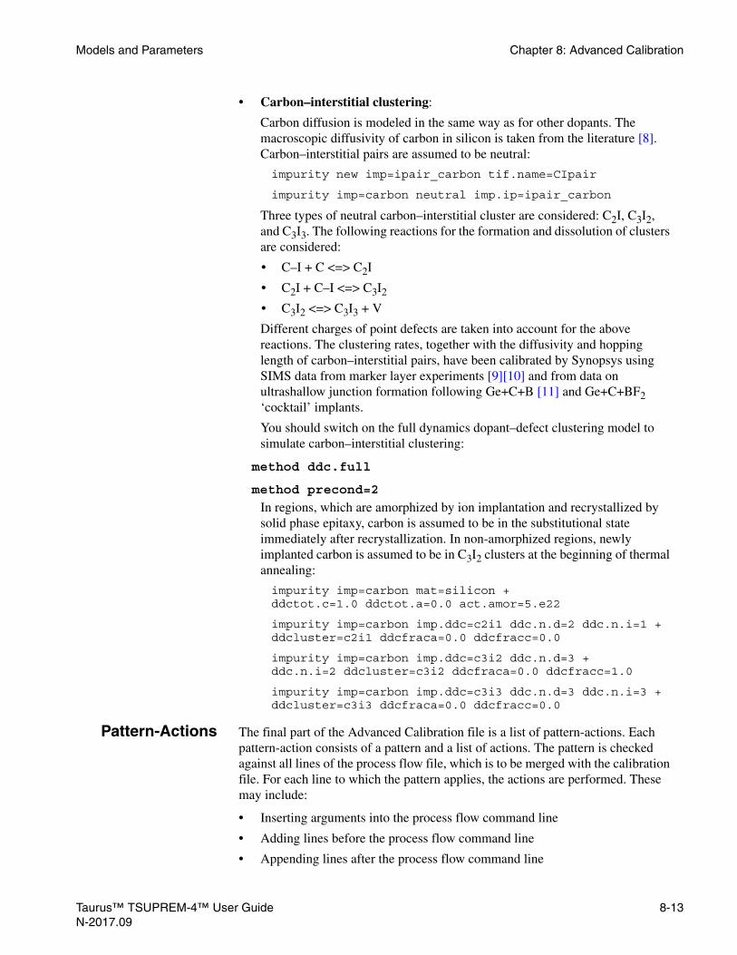
Models and Parameters Chapter 8: Advanced Calibration

• Carbon–interstitial clustering:

Carbon diffusion is modeled in the same way as for other dopants. The macroscopic diffusivity of carbon in silicon is taken from the literature [8]. Carbon–interstitial pairs are assumed to be neutral:

impurity new imp=ipair_carbon tif.name=CIpair

impurity imp=carbon neutral imp.ip=ipair_carbon

Three types of neutral carbon–interstitial cluster are considered: C2I, C3I2, and C3I3. The following reactions for the formation and dissolution of clusters are considered:

• C–I + C <=> C2I

• C2I + C–I <=> C3I2

• C3I2 <=> C3I3 + V

Different charges of point defects are taken into account for the above reactions. The clustering rates, together with the diffusivity and hopping length of carbon–interstitial pairs, have been calibrated by Synopsys using SIMS data from marker layer experiments [9][10] and from data on ultrashallow junction formation following Ge+C+B [11] and Ge+C+BF2 ‘cocktail’ implants.

You should switch on the full dynamics dopant–defect clustering model to simulate carbon–interstitial clustering:

method ddc.full

method precond=2

In regions, which are amorphized by ion implantation and recrystallized by solid phase epitaxy, carbon is assumed to be in the substitutional state immediately after recrystallization. In non-amorphized regions, newly implanted carbon is assumed to be in C3I2 clusters at the beginning of thermal annealing:

impurity imp=carbon mat=silicon +ddctot.c=1.0 ddctot.a=0.0 act.amor=5.e22

impurity imp=carbon imp.ddc=c2i1 ddc.n.d=2 ddc.n.i=1 +ddcluster=c2i1 ddcfraca=0.0 ddcfracc=0.0

impurity imp=carbon imp.ddc=c3i2 ddc.n.d=3 +ddc.n.i=2 ddcluster=c3i2 ddcfraca=0.0 ddcfracc=1.0

impurity imp=carbon imp.ddc=c3i3 ddc.n.d=3 ddc.n.i=3 +ddcluster=c3i3 ddcfraca=0.0 ddcfracc=0.0

Pattern-Actions The final part of the Advanced Calibration file is a list of pattern-actions. Each pattern-action consists of a pattern and a list of actions. The pattern is checked against all lines of the process flow file, which is to be merged with the calibration file. For each line to which the pattern applies, the actions are performed. These may include:

• Inserting arguments into the process flow command line

• Adding lines before the process flow command line

• Appending lines after the process flow command line

Taurus™ TSUPREM-4™ User Guide 8-13N-2017.09

Chapter 8: Advanced Calibration Models and Parameters

The patterns and actions supported by the Merger application are explained in the Advanced Calibration for Process Simulation User Guide [1]. In this section, the pattern-actions of AdvCal_1d_tables_2008.09.smr are explained, following the order in the Advanced Calibration file. Most pattern-actions are used to set initial conditions after ion implantation, such as the amount of interstitials created by the implant or the initial activation of dopants.

DepositionPattern-Action

Only the first pattern-action is applied to deposition steps:

# Sets spacing in deposited oxide

Condition (1) if ( line && "DEPOSITION" ) {insert {dy=0.0005}

}

The Merger application will search for all deposition commands in the TSUPREM-4 input file and will insert the string "dy=0.0005".

Pattern-Actions forAs-Implanted

Profiles

In the Advanced Calibration file, the implantation dose is interpreted as the dose per the wafer area. This is performed by the following pattern-action:

Condition (1) if ( implantation && element!=silicon ) {insert {dose.sca}

}

Note:If you need to interpret the implant dose as the dose per the wafer area of the implant beam must deactivate this pattern-action by changing Condition (1) to Condition (0).

The next pattern-action sets the parameters for Monte Carlo ion implantation. By default, this pattern-action is deactivated by Condition (0):

Condition (0) if ( implantation ) {insert {montecarlo n.ion=5000 dose.spl traj.spl}

}

Two pattern-actions are dedicated to the implantation of silicon ions, for which no calibrated implantation lookup tables are available. For energies greater than 5 keV, phosphorus tables are used because phosphorus ions have a mass similar to silicon ions. For energies less than 5 keV, Monte Carlo simulation is used for silicon implantation.

Pattern-Actions forInitial Conditions

After Implant

Most pattern-actions are dedicated to setting the initial conditions after ion implantation. The parameters are set depending on the implant species and, in some cases, also as a function of implant energy and dose. In particular, the following two parameters are set:

• act.amor: The maximum active concentration of the implanted dopants in amorphized regions. If the dopant concentration exceeds act.amor, the surplus is put into dopant clusters.

8-14 Taurus™ TSUPREM-4™ User GuideN-2017.09

Models and Parameters Chapter 8: Advanced Calibration

• c1.ini.f: The fraction of dopants that is clustered in nonamorphized regions.

Furthermore, for all dopants, act.ni=0 and c1frac.a=1. All dopants that are in clusters after ion implantation should be in transient dopant–defect clusters. This is a logical consequence of switching off the other clusters of the dopant activation model act.full.

Complex Models A set of complex models can be invoked by typing the following command

method advanced version=2013.12.a

or uncommenting the corresponding line in the startblock. The file s4advanced.2013.12.a will be sourced in this case. That file contains calibrated parameters for the following models:

• Complex interstitial clustering model taking SMICs and {311} defect formation into account

• Boron-interstitial clustering (BICs) model

• Arsenic-vacancy clustering model

The model parameters were translated from the 2008 version of the Advanced Calibration for Sentaurus Process (AdvancedModels mode) [1]. The five-stream pair diffusion model is used along with the above models when the complex model mode is selected.

Switching on the complex models results in a significant CPU time increase because of increased total number of equations to be solved. Therefore, using the complex models is recommended in the case when the basic set models can not predict the experimentally observed trends (flash lamp, laser, low-temperature annealing) as well as for the fundamental research.

ComplexInterstitial

Clustering Model

The advanced interstitial clustering model includes three equations for small interstitial clusters (I2, I3, I4) and two equations for the density of {311} defects and density of interstitials bound in {311} defects (2 moments) [12]. Select it with the following command:

interstitial silicon cl.full cl.2m

The high interstitial supersaturation in the initial TED stage can be reproduced using the advanced model. A comparison of simulation and experimental results is shown in Figure 8-1 for silicon implantation and subsequent annealing at different temperatures. The model accurately predicts two TED stages observed for low temperatures.

Interstitials generated by the implantation are assumed to be in the free state in the beginning of annealing when the complex model is used. It is different from the basic 1Moment model for which excess interstitials are assumed to be mostly bound in {311} defects at the initial annealing stage.

Taurus™ TSUPREM-4™ User Guide 8-15N-2017.09

Chapter 8: Advanced Calibration Models and Parameters

Figure 8-1 Interstitial supersaturation as a function of annealing time. Silicon was implanted at 40 keV with a dose of 2 x 1013 cm–2. Annealing was performed at 600oC (red), 700oC (blue) and 800oC (black). There is a good agreement between simulations (solid lines) and experiments (squares). Experimental data points are extracted from [13].

BICs Model According to the implemented model, there are six types of BICs: B2, B2I, B2I2, B3I, B3I2, B3I3. All the clusters are neutral. An example of B2I2 definition is as follows:

impurity imp=bor2i2 tif.name=B2I2 new neutral c.init=1.e2

impurity imp=boron imp.ddc=bor2i2 ddc.n.d=2 +ddc.n.i=2ethod precond=2

The dopant-defect clustering full-dynamics(ddc.full)model is switched on to simulate the BICs growth, and the formation of single clusters used in the basic model set is switched off:

method ddc.full

impurity mater=silicon imp=boron cm.sec + ddcf.i.n=0 ddcr.i.n=0 ifracm=0 ddcf.d.n=0 +ddcf.n.n=0 ddcr.n.n=0 ddc.f.0=0.0 ddc.f.e=0.0 +ddc.t.0=0.0 ddc.t.e=0.0

800ºC, simulation800ºC, experiment700ºC, simulation700ºC, experiment600ºC, simulation600ºC, experiment

Time [s]100 101 102 103 104 105

Inte

rstit

ial S

uper

satu

ratio

n

100

101

102

103

104

105

106

107

108

8-16 Taurus™ TSUPREM-4™ User GuideN-2017.09

Models and Parameters Chapter 8: Advanced Calibration

Note:Since ddc.full model is activated, the carbon-interstitial clustering model is always used when the complex model set is chosen.

The reaction pathway is presented in Figure 8-2. The most stable clusters are B3I and B3I2. All the charge states of point defects and boron-point defect pairs are taken into account in the model. The reaction rates are determined by the parameters ddc.kf.0, ddc.kf.e, ddc.eq.0, ddc.eq.e:

$ B2I1 + I <-> B2I2

impurity imp=boron mat=silicon +ddc.r=bor2i2 i.ddc c.i.all +ddc.kf.0=2.6094e-5 ddc.kf.e=1.77 +ddc.eq.0=1.0 ddc.eq.e=-0.132 cm.sec

Figure 8-2 Reaction pathway for the BICs model.

The initial boron activation level after implantation is defined using the parameters act.amor, ddctot.c similarly to the basic model set method. The initial concentration of different type clusters in the amorphized and crystalline silicon are calculated according the parameter ddcfracc and ddcfraca respectively. By default, those parameters are equal to 1.0 for B2 and for other BICs.

Arsenic-VacancyClustering Model

The arsenic-vacancy clustering model implementation is similar to the BICs model one. Formation of six type clusters are considered: As2, As2V, As3, As3V, As4, As4V. The most stable clusters are As4V. The clustering reactions are chosen according to the model published by Pinacho et al. [14]. The reaction pathway is presented in Figure 8-3.

B B2I

B2

B3I

B3I2

B3I3

B2I2BI

BI

I,V

I,V

BI

BI

BI

BI

I,V

I,V

105–

Taurus™ TSUPREM-4™ User Guide 8-17N-2017.09

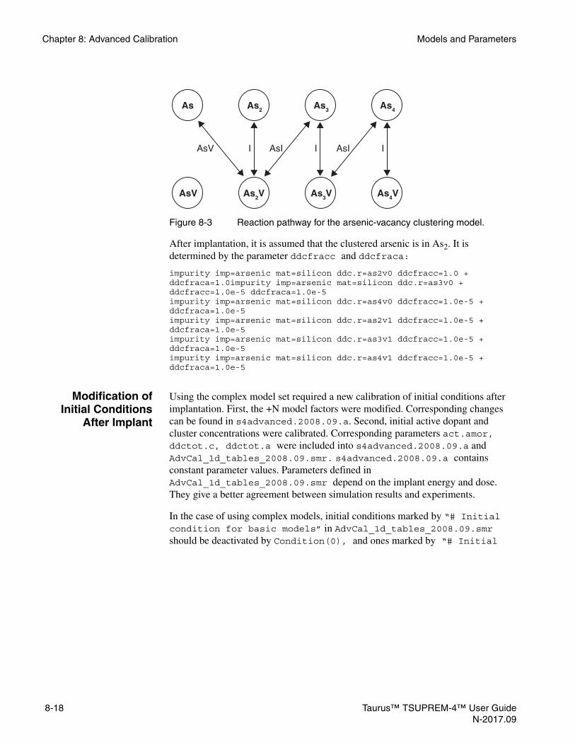
Chapter 8: Advanced Calibration Models and Parameters

Figure 8-3 Reaction pathway for the arsenic-vacancy clustering model.

After implantation, it is assumed that the clustered arsenic is in As2. It is determined by the parameter ddcfracc and ddcfraca:

impurity imp=arsenic mat=silicon ddc.r=as2v0 ddcfracc=1.0 +ddcfraca=1.0impurity imp=arsenic mat=silicon ddc.r=as3v0 +ddcfracc=1.0e-5 ddcfraca=1.0e-5impurity imp=arsenic mat=silicon ddc.r=as4v0 ddcfracc=1.0e-5 +ddcfraca=1.0e-5impurity imp=arsenic mat=silicon ddc.r=as2v1 ddcfracc=1.0e-5 +ddcfraca=1.0e-5impurity imp=arsenic mat=silicon ddc.r=as3v1 ddcfracc=1.0e-5 +ddcfraca=1.0e-5impurity imp=arsenic mat=silicon ddc.r=as4v1 ddcfracc=1.0e-5 +ddcfraca=1.0e-5

Modification ofInitial Conditions

After Implant

Using the complex model set required a new calibration of initial conditions after implantation. First, the +N model factors were modified. Corresponding changes can be found in s4advanced.2008.09.a. Second, initial active dopant and cluster concentrations were calibrated. Corresponding parameters act.amor, ddctot.c, ddctot.a were included into s4advanced.2008.09.a and AdvCal_1d_tables_2008.09.smr. s4advanced.2008.09.a contains constant parameter values. Parameters defined in AdvCal_1d_tables_2008.09.smr depend on the implant energy and dose. They give a better agreement between simulation results and experiments.

In the case of using complex models, initial conditions marked by “# Initial condition for basic models” in AdvCal_1d_tables_2008.09.smr should be deactivated by Condition(0), and ones marked by “# Initial

As As2As3

AsII AsIAsV I I

As4As3

AsV As2V As3V As4V

8-18 Taurus™ TSUPREM-4™ User GuideN-2017.09

Guidelines for Additional Calibration Chapter 8: Advanced Calibration

condition for complex models” should be switched on by Condition(1). For example:

# Initial condition for basic modelsCondition (0) if ( implantation && element==arsenic ) {prepend {impurity impurity=arsenic mat=silicon act.ni=0.0 +c1frac.a=1.0 +act.amor=2.0e20*($energy+0.5)/$energy c1.ini.f=0.6 ddctot.c=0.6}}# Initial condition for complex modelsCondition (1) if ( implantation && element==arsenic ) {prepend {impurity impurity=arsenic mat=silicon act.ni=0.0 +act.amor=1.5e21*$energy/($energy+10.0)*($dose+1.e14)/+($dose+3.e14) ddctot.c=1.0}}

Guidelines for Additional CalibrationThe Advanced Calibration file is a starting point for accurate process simulation with TSUPREM-4. However, the Advanced Calibration cannot fully replace an additional calibration by the user for 2D applications. With a customized process calibration, the accuracy can always be further increased for any technology of interest. You must perform a customized calibration of the process and device simulation models or you can request one from Synopsys in the context of a customer service project.

To further improve the Advanced Calibration, Synopsys appreciates feedback from customers regarding the accuracy obtained with the parameter files for different process conditions and suggestions for improved models or parameter values.

The Advanced Calibration of TSUPREM-4 is widely based on the 2008 version of the Advanced Calibration of Sentaurus Process [1]. Therefore, the part of the Advanced Calibration for Process Simulation User Guide which is dedicated to process simulation with Sentaurus Process, also widely applies to the Advanced Calibration of TSUPREM-4 and is recommended for reading.

Limitations of the Advanced Calibration of TSUPREM-4 are described and the most important tuning parameters for standard applications are summarized.

All changes should be performed by editing the Advanced Calibration file of TSUPREM-4. To do so, make a local copy of AdvCal_1d_tables_2008.09.smr, rename it, and use the Merger GUI or a text editor to change models, parameters, or pattern-actions in the local copy. The default version of AdvCal_1d_tables_2008.09.smr is located in the TSUPREM-4 library.

Taurus™ TSUPREM-4™ User Guide 8-19N-2017.09

Chapter 8: Advanced Calibration Guidelines for Additional Calibration

Accuracy and Limitations of Advanced Calibration of TSUPREM-4

The Advanced Calibration of TSUPREM-4 has the same average accuracy as the Advanced Calibration of Sentaurus Process:

• Oxidation-enhanced diffusion (OED) may be overestimated for wet oxidation.

• Interstitial trapping by fluorine atoms cannot be simulated.

• Parameters of the arsenic and phosphorus activation models are not well calibrated for extremely high concentrations (close to ) and low temperatures.

• There may be a significant difference between simulation results and experimental data in the case of co-diffusion of arsenic and phosphorus.

• Indium redistribution during annealing after amorphizing implantation cannot be simulated correctly.

Fine-Tuning Parameters

The Advanced Calibration provides a good starting point for accurate process simulation. However, to match the simulation results precisely with experimental data, an additional fine-tuning of the models is helpful. In total, many parameters are used in the models.

This section gives recommendations as to which parameters to use for additional calibration. Table 8-1 summarizes the fine-tuning parameters. (Essentially, the recommendations are the same as those for the additional calibration of Sentaurus Process [1], but the parameters are different in TSUPREM-4).

1022

cm3–

Table 8-1 Fine-tuning Parameters in TSUPREM-4 of TSUPREM-4

TSUPREM-4 Parameters Sentaurus Process Analogue Recommended Use

theta.0, theta.e theta OED calibration.

cl.kr.0, cl.kr.e Ikr TED calibration. Adjustment of the diffusion profile tail.

r.i.s, e.i.s, r.v.s,e.v.s

kfKickOut Adjustment of the dopant profile tail in the case of using the five-stream diffusion model.

ddc.t.0, ddc.t.e CluRate (~1/ddc.t) Adjustment of B diffusion profiles in the high and medium concentration regions.

q.max.0, q.max.e CMax Adjustment of As and P diffusion pro-file depth and concentration level at the interface.

d.plus ifactor Final fitting in the tail region.

8-20 Taurus™ TSUPREM-4™ User GuideN-2017.09

Guidelines for Additional Calibration Chapter 8: Advanced Calibration

Point-DefectParameters

The basic point-defect parameters (diffusivities, equilibrium concentration, and charge states) influence the simulation results of all dopants. Therefore, it is not recommended to tune them for the purpose of improving the accuracy of the diffusion of one particular dopant.

The only recommended point defect calibration parameter is the fraction of consumed silicon atoms that are injected as interstitials during oxidation (theta.0, theta.e). To adjust OED in different ambients, edit the following line containing the default values:

interstitial silicon /oxide theta.0=7.3e4 +theta.e=2.1

Interstitial Clusters TED after ion implantation is described by the one-moment model for interstitial clusters. This model is simple and fast, but still accurate enough for most applications. For a discussion of the limitations of this model, see the Advanced Calibration for Process Simulation User Guide [1]. Within this model, the best way of tuning the time and temperature dependence of TED is the adjustment of the cluster dissolution rate. It can be performed by changing the default parameter values in the line below:

interstitial silicon cl.kr.0=6.996e16 +cl.kr.e=3.935

kr.0 and cl.kr.e correspond to the parameter Ikr in Sentaurus Process.

DopantParameters

The following section describes dopant parameters which can be used for the additional calibration.

Diffusion TED after ion implantation can be modified by increasing or lowering the number of interstitials generated by dopant implant. Such a modification needs to be performed by editing the formulas for the calculation of the parameter d.plus in the pattern-actions section. Increasing the number of interstitials generated by an implant will mainly increase the diffusion in the tail of the dopant profile.

If the five-stream model is used, the capture radius and the energy barrier for the formation of dopant–defect pairs are critical parameters, which govern the average migration length between pair formation and pair dissolution. Therefore, in the five-stream model, to adjust the average pair migration length, change the parameters r.i.s, e.i.s, r.v.s, and e.v.s. This can be performed for each charge state separately.

act.amor AmInit Final fitting in the high concentration region.

c1.ini.f AcInit Final fitting in the medium concentra-tion region.

Table 8-1 Fine-tuning Parameters in TSUPREM-4 of TSUPREM-4

TSUPREM-4 Parameters Sentaurus Process Analogue Recommended Use

Taurus™ TSUPREM-4™ User Guide 8-21N-2017.09

Chapter 8: Advanced Calibration Guidelines for Additional Calibration

For example, you can define the capture radius value for neutral B–I pairs in the following line:

impurity imp=boron mater=silicon c.inter=1 +r.i.s=6.68e-1

The Advanced Calibration TSUPREM-4 file does not contain any special models for the diffusion of P in regions with a very high As concentration. The simulation of the co-diffusion of As and P is not very accurate for all possible conditions. One method to tune P diffusion in regions of high As concentration is to introduce diffusion enhancement coefficients for P–I and P–V pairs, which depend on the local As concentration. The corresponding TSUPREM-4 commands are:

impurity imp=phosphorus mater=silicon di.fac=...

impurity imp=phosphorus mater=silicon dv.fac=...

where "..." must be some function of the local arsenic concentration, which has the value of 1 for low arsenic concentration.

Activation The same dopant activation model is used as in the Advanced Calibration of Sentaurus Process. The rate of cluster dissolution is the most widely used parameter for the fine-tuning of the junction depth of boron ultrashallow junctions. Its influence is illustrated in Figure 8-4.

Figure 8-4 Effect of boron cluster dissolution time prefactor ddc.t.0 on final shape of a boron profile after 2 keV 2 x 1015 cm–2 boron implantation and spike annealing at 1050oC

ddc.t.0 = 3.2 x 10–20

ddc.t.0 = 8.0 x 10–21 (default)ddc.t.0 = 2.0 x 10–21

Depth [nm]0 50 100

Bor

on [c

m–3

]

1017

1018

1019

1020

1021

8-22 Taurus™ TSUPREM-4™ User GuideN-2017.09

Guidelines for Additional Calibration Chapter 8: Advanced Calibration

To adjust the clustering rate, modify the cluster dissolution time values defined by ddc.t.0 and ddc.t.e:

impurity mater=silicon imp=boron +ddc.t.0=8.0e-21 ddc.t.e=-4.7

The cluster dissolution time is inversely proportional to the cluster dissolution rate defined by the parameter CluRate in Sentaurus Process.

For PMOS extension formation after BF2 implant, where the temperature cycle often includes a nitride spacer deposition at followed by a spike anneal, it may be necessary to increase the cluster dissolution time significantly.

Segregation Additional fine-tuning of dopant dose loss becomes important in the case of ultrashallow junction formation simulation. The maximum trap density in the Si–SiO2 interface defined by q.max.0 and q.max.e is the most powerful calibration parameter for such an adjustment. That parameter is widely used to change the simulated depth of arsenic and phosphorus diffusion profiles. An example of the definition of the maximum phosphorus trap density is:

impurity impurity=i_phosphorus +mat=oxide /mat=silicon q.max.0=1.8e15

Increasing the trap density results in shallower simulated diffusion profiles as shown in Figure 8-5.

Figure 8-5 Effect of q.max.0 on simulation results for phosphorus USJ formation; graphs were calculated for 2 keV 1015 cm–2 P implantation, followed by a spike anneal at 1080oC

700°C

q.max.0 = 1.8 x 1015 (default)q.max.0 = 6.0 x 1014

q.max.0 = 3.0 x 1014

Depth [nm]0 50 100

Pho

spho

rus

[cm

-3]

1016

1017

1018

1019

1020

Taurus™ TSUPREM-4™ User Guide 8-23N-2017.09

Chapter 8: Advanced Calibration Guidelines for Additional Calibration

Indium Dose Loss The calibration of indium diffusion and dose loss is very accurate for non-amorphizing conditions and usually does not require additional fine-tuning.

For high-dose indium implantation, the accuracy is limited. TSUPREM-4 offers a very simple, but effective way to adjust the indium dose loss after high-dose indium implantation. You can cut off the indium concentration in amorphized regions by setting the parameter max.amor, for example:

impurity mat=silicon imp=indium max.amor=7e18

As-ImplantedDopant Profiles

By default, the Taurus implantation tables are used for the calculation of as-implanted dopant profiles. These are very accurate for most implantation conditions.

For ion implants with energy less than 5 keV, the Sentaurus Process implant tables give a better accuracy in most cases. However, these have a different format and are not provided in the TSUPREM-4 libraries. A translation of the Sentaurus Process implant tables to the TSUPREM-4 readable format is available from Synopsys upon request.

For highly accurate 2D profiles in arbitrary device geometries, Monte Carlo implantation can be used.

Polysilicon The TSUPREM-4 file does not include a calibration of the dopant diffusion in polysilicon and the out-diffusion of dopants from polysilicon.

DopantPenetration

Through GateOxide

The dopant penetration through gate oxide has not been calibrated. This is a difficult task because, instead of pure oxide, oxynitride is commonly used as the gate dielectric material. You can completely suppress the dopant diffusion from polysilicon through the gate oxide into the channel region by setting the transfer coefficient at the polysilicon–oxide interface to 0.

8-24 Taurus™ TSUPREM-4™ User GuideN-2017.09

References Chapter 8: Advanced Calibration

References[1] Advanced Calibration for Process Simulation User Guide, Version

J-2014.09, Mountain View, California: Synopsys Inc., 2014.

[2] F. J. Morin and J. P. Maita, “Electrical Properties of Silicon Containing Arsenic and Boron,” Physical Review, vol. 96, no. 1, pp. 28–35, 1954.

[3] P. A. Stolk et al., “Physical mechanisms of transient enhanced dopant diffusion in ion-implanted silicon,” Journal of Applied Physics, vol. 81, no. 9, pp. 6031–6050, 1997.

[4] H. Saleh et al., “Energy dependence of transient enhanced diffusion and defect kinetics,” Applied Physics Letters, vol. 77, no. 1, pp. 112–114, 2000.

[5] S. T. Dunham and C. D. Wu, “Atomistic models of vacancy-mediated diffusion in silicon,” Journal of Applied Physics, vol. 78, no. 4, pp. 2362–2366, 1995.

[6] A. N. Larsen et al., “Heavy doping effects in the diffusion of group IV and V impurities in silicon,” Journal of Applied Physics, vol. 73, no. 2, pp. 691–698, 1993.

[7] V. C. Venezia et al., “Dopant redistribution effects in preamorphized silicon during low temperature annealing,” in IEDM Technical Digest, Washington, DC, USA, pp. 489–492, December 2003.

[8] P. Pichler, Intrinsic Point Defects, Impurities, and Their Diffusion in Silicon, Computational Microelectronics, Vienna: Springer, 2004.

[9] H. Rücker et al., “Suppressed diffusion of boron and carbon in carbon-rich silicon,” Applied Physics Letters, vol. 73, no. 12, pp. 1682–1684, 1998.

[10] P. Lavéant et al., “Engineering the diffusion behavior of dopants (B, Sb) in silicon by incorporation of carbon,” Nuclear Instruments and Methods in Physics Research B, vol. 186, no. 1–4, pp. 292–297, 2002.

[11] V. Moroz et al., “Optimizing boron junctions through point defect and stress engineering using carbon and germanium co-implants,” Applied Physics Letters, vol. 87, p. 051908, August 2005.

[12] C. Zechner et al., “Accurate and efficient TCAD model for the formation and dissolution of small interstitial clusters and {311} defects in silicon,” Materials Science and Engineering B, vol. 124–125, pp. 401–403, December 2005.

[13] N. E. B. Cowern et al., “Energetics of Self-Interstitial Clusters in Si,” Physical Review Letters, vol. 82, no. 22, pp. 4460–4463, 1999.

[14] R. Pinacho et al., “Modeling arsenic deactivation through arsenic-vacancy clusters using an atomistic kinetic Monte Carlo approach,” Applied Physics Letters, vol. 86, p. 252103, June 2005.

Taurus™ TSUPREM-4™ User Guide 8-25N-2017.09

Chapter 8: Advanced Calibration References

8-26 Taurus™ TSUPREM-4™ User GuideN-2017.09

APPENDIX A

Default CoefficientsA

Default Coefficient ValuesThis appendix contains the values of the various simulation coefficients used in TSUPREM-4, along with the references from which the values were obtained. In some cases, there are also notes regarding the approximations that were made when the necessary values had not been experimentally determined or when there was wide scatter in the available data. These notes regarding the approximations involved in the coefficient determination should help you know how much latitude is available when modifying these coefficients to match fabrication results. The units for the coefficients are given in Chapter 4; where a choice of units is available, the default units (that is, microns and minutes) are used, except as noted.

The notes referenced in this section are described in Notes, p. A-32. They appear in the form “(1),” in which the digit is the number of the note in the list of notes.

Tables Page

Impurity Parameters A-2Impurity Diffusion Coefficients A-2Segregation and Transport Coefficients A-5Polysilicon Grain Segregation A-7Clustering and Solid Solubility A-7Point Defect Parameters A-9Oxidation A-12Diffusion Enhancement Oxides A-16Silicidation A-16Analytical Implant A-18Monte Carlo (MC) Implant A-19Electrical Parameters A-20Material Coefficients A-22Numerical Methods A-25Automatic Grid Generation Parameters A-26Adaptive Grid Parameters A-27Grid Parameters A-28

Taurus™ TSUPREM-4™ User Guide A-1N-2017.09

Appendix A: Default Coefficients Default Coefficient Values

The references listed in this section are described in References, p. A-28. They appear in the form “[1],” in which the digit is the number of the reference in the list of references.

Impurity Parameters

Impurity Diffusion Coefficients

Diffusivities are in μm2/min except as noted.

Table A-1 Impurity Parameters (Silicon Dopants)

Boron Phosphorus Arsenic Indium Antimony

TIF.NAME B P As In Sb

Type ACCEPTOR DONOR DONOR ACCEPTOR DONOR

Implant table chboron dual.pho dual.ars tr.indium antimony

AT.NUM 5.0 15.0 33.0 49.0 51.0

AT.WT 10.8 30.97 74.91 115 121.76

Table A-2 Impurity Parameters (Other)

Aluminum Fluorine Nitrogen Silicon

TIF.NAME Al F N Si

AT.NUM 13.0 9.0 7.0

AT.WT 26.98 18.9984 14.01

Table A-3 Impurity Diffusion Coefficients

Boron Phosphorus Arsenic Indium Antimony Fluorine Germanium Nitrogen

Silicon (1)DIP.0 4.10e9 [1] 0 [1]0000 0 [2]00 0 (2) 0 [1] 0 0 0

DIP.E 3.46 0.00 0.000 00000 00000 0 0 0

DIX.0 2.11e8 2.31e10 1.37e700

1.8

cm2/s

6.420e7 4.23e3

cm2/s

80.0

cm2/s

0.05

cm2/s

DIX.E 3.46 3.66 3.44 3.6 3.65 3.5 4.7 3.65

DIM.0 0/00 2.664e10 3.72e10 0 4.50e9 0 0 0

DIM.E 0.00 4.00 4.15 0 4.08 0 0 0

DIMM.0 0.00 2.652e11 0.00 000 000 0 0 0

DIMM.E 0.00 4.37 0.00 000 000 0 0 0

DVP.0 2.16e8 0.00 0.00 000 000 0 0 0

DVP.E 3.46 0.00 0.00 000 000 0 0 0

DVX.0 1.11e7 0.00 5.47e7 0 1.220e9 0 320.0

cm2/s

0

DVX.E 3.46 3.66 3.44 0 3.65 0 0 0

DVM.0 0.00 0.00 1.49e11 0 8.55e10 0 0 0

DVM.E 0.00 4.00 4.15 0 4.08 0 0 0

DVMM.0 0.00 0.00 0.00 000 000 0 0 0

DVMM.E 00.0 4.37 0.00 000 000 0 0 0

VD 4.4.00 10.0.00 -13.2 0 -13.0 0 -13.0 0

A-2 Taurus™ TSUPREM-4™ User GuideN-2017.09

Default Coefficient Values Appendix A: Default Coefficients

VMIPAIR 4.4 10.0 -13.2 0 -13.0 0 -13.0 0

VMVPAIR 4.4 10.0 -13.2 0 -13.0 0 -13.0 0

VFSUB 0 0 0 0 0 0 0 0

VALPHAM 0 0 0 0 0 0 0 0

VFIPAIR 0 0 0 0 0 0 0 0

VALPHAN 0 0 0 0 0 0 0 0

VFVPAIR 0 0 0 0 0 0 0 0

Oxide [8] (3)DIX.0 1.896e6 4.338e10 1.05e10 18. 7.86e25 2.858 1.05e10 0.05

DIX.E 3.53 4.44 4.89 3.6 8.75 3.5 4.89 3.65

Polysilicon (grain interior) (diffusivities in cm2/s) (4)DIP.0 0.72 0..00 0.00 0.00 0.00 0 0 0

DIP.E 3.46 0.00 0.00 0.00 0.00 0 0 0

DIX.0 0.037 3.85 1.14e-2 1.8 0.214 1.70e5 1.14e-2 0.05

DIX.E 3.46 3.66 3.44 3.6 3.65 3.5 3.44 3.65

DIM.0 0.00 4.44 31.000 00 15.000 0 0 0

DIM.E 0.00 4.00 4.15 0 4.08 0 0 0

DIMM.0 0.00 44.200 7.17e3 000 000 0 0 0

DIMM.E 0.00 4.37 5.21 000 000 0 0 0

Polysilicon (grain boundaries) (diffusivities in cm2/s) (5)DIX.0 420. 6.0e3 110.0000 0 2.14e3 0 0 0

DIX.E 3.46 3.66 3.53 0 3.65 0 0 0

DIM.0 0.00 0.00 10.000 000 000 0 0 0

DIM.E 0.00 0.00 3.53 000 000 0 0 0

TiSi2 (diffusivities in cm2/s)

DIX.0 6.0e-7 4.6e-6 4.0e-7 00 7.0e-80 0 4.0e-7 0

DIX.E 2.0 2.00 1.8 0 1.8 0 1.8 0

CoSi2 (diffusivities in cm2/s)

DIX.0 1.64e-2 8.0e-5 7.37 1.64e-2 7.370 0 4.0e-7 0

DIX.E 2.05 2.050 3.3 2.05 3.3 0 1.8 0

WSi2 (diffusivities in cm2/s) (6) [9]-[12]DIX.0 1.0e-5 4.20e-2 2.60e-2 00 2.60e-20 0 2.60e-2 0

DIX.E 1.17 2.14 2.11 0 2.11 0 2.11 0

Ambient (7)DIX.0 1e130 1e13. 5e13 180.. 5e13. 1e13 5e13 5.0DIX.E 3.500 3.50 3.95 3.6 3.95 3.5 3.95 3.65

Table A-3 Impurity Diffusion Coefficients (Continued)

Boron Phosphorus Arsenic Indium Antimony Fluorine Germanium Nitrogen

Table A-4 Other Impurities and Materials

DIP.0 0

DIP.E 0

DIX.0 0

DIX.E 0

DIM.0 0

DIM.E 0

Taurus™ TSUPREM-4™ User Guide A-3N-2017.09

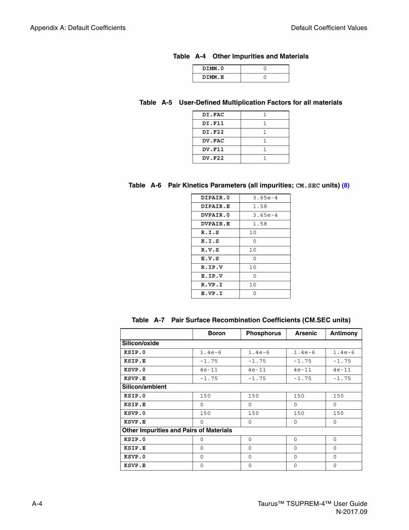
Appendix A: Default Coefficients Default Coefficient Values

DIMM.0 0

DIMM.E 0

Table A-5 User-Defined Multiplication Factors for all materials

DI.FAC 1

DI.F11 1

DI.F22 1

DV.FAC 1

DV.F11 1

DV.F22 1

Table A-6 Pair Kinetics Parameters (all impurities; CM.SEC units) (8)

DIPAIR.0 3.65e-400

DIPAIR.E 1.58

DVPAIR.0 3.65e-4

DVPAIR.E 1.58

R.I.S 10000

E.I.S 000

R.V.S 10000

E.V.S 000

R.IP.V 10000

E.IP.V 000

R.VP.I 10000

E.VP.I 000

Table A-7 Pair Surface Recombination Coefficients (CM.SEC units)

Boron Phosphorus Arsenic Antimony

Silicon/oxide KSIP.0 1.4e-6 1.4e-6 1.4e-60 1.4e-6

KSIP.E -1.75 -1.75 -1.75 -1.75

KSVP.0 4e-11 4e-11 4e-11 4e-11

KSVP.E -1.75 -1.75 -1.75 -1.75

Silicon/ambientKSIP.0 150 150 1500 150

KSIP.E 0 0 0 0

KSVP.0 150 150 150 150

KSVP.E 0 0 0 0

Other Impurities and Pairs of MaterialsKSIP.0 0 0 00 0

KSIP.E 0 0 0 0

KSVP.0 0 0 0 0

KSVP.E 0 0 0 0

Table A-4 Other Impurities and Materials

A-4 Taurus™ TSUPREM-4™ User GuideN-2017.09

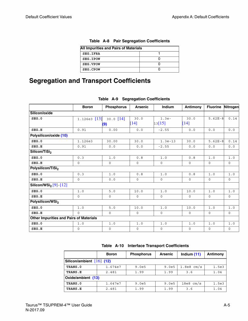
Default Coefficient Values Appendix A: Default Coefficients

ogen

.14

.0

.14

.0

.0

.0

.0

.0

.0

Segregation and Transport Coefficients

Table A-8 Pair Segregation Coefficients

All Impurities and Pairs of MaterialsSEG.IFRA 1

SEG.IPOW 0SEG.VPOW 0

SEG.CPOW 0

Table A-9 Segregation Coefficients

Boron Phosphorus Arsenic Indium Antimony Fluorine Nitr

Silicon/oxide SEG.0 1.126e3 [13] 30.0 [14]

(9)

30.0

[14]01.3e-

13[15]30.0

[14]5.62E-8 0

SEG.E 0.91000 0.00 0.0 -2.55 0.0 0.0 0

Polysilicon/oxide (10)SEG.0 1.126e3 30.00 30.00 1.3e-13 30.00 5.62E-8 0

SEG.E 0.9100 0.0 0.0 -2.55 0.0 0.0 0

Silicon/TiSi2SEG.0 0.3000 1.0 0.80 1.0 0.8 1.0 1

SEG.E 0000.0 0.0 0.0 0.0 0.0 0 0

Polysilicon/TiSi2SEG.0 0.3000 1.0 0.8 1.0 0.8 1.0 1

SEG.E 000.00 0.0 0.0 0.0 0.0 0 0

Silicon/WSi2 [9]-[12]SEG.0 1.0000 5.0 10.00 1.0 10.0 1.0 1

SEG.E 0000.0 0.0 0.0 0..0 0..0 0 0

Polysilicon/WSi2SEG.0 1.0000 5.0 10.00 1.0 10.0 1.0 1

SEG.E 0000.0 0.0 0.0 00 00 0 0

Other Impurities and Pairs of MaterialsSEG.0 1.0000 1.00 1.00 1.00 1.00 1.0 1

SEG.E 000000 00 00 00 00 0 0

Table A-10 Interface Transport Coefficients

Boron Phosphorus Arsenic Indium (11) Antimony

Silicon/ambient [16] (12)TRANS.0 1.674e7 9.0e5 9.0e5 1.8e8 cm/s 1.5e3

TRANS.E 2.481 1.99 1.99 3.6 1.04

Oxide/ambient (13)TRANS.0 1.647e7 9.0e5 9.0e5 18e8 cm/s 1.5e3

TRANS.E 2.481 1.99 1.99 3.6 1.04

Taurus™ TSUPREM-4™ User Guide A-5N-2017.09

Appendix A: Default Coefficients Default Coefficient Values

Polysilicon/ambient (13)TRANS.0 1.674e7 9.0e5 9.0e5 1.8e8 cm/s 1.5e3

TRANS.E 2.481 1.99 1.99 3.6 1.04

Polysilicon/silicon (14)TRANS.0 100.000 100.00 100.000 1.8e8 cm/s 100.000

TRANS.E 0.0 0.0 0.00 3.6 0.0

Silicon/oxide and Polysilicon/oxideTRANS.0 0.1000 0.10 0.100 1.8e8 cm/s 0.100

TRANS.E 0.0 0.0 0.00 3.6 0.0

All materials With Nitride and OxynitrideTRANS.0 00 0 0 0 0000

TRANS.E 0.0 0.0 0.00 3.6 0.0

Silicon/TiSi2

TRANS.0 1.0e6 1.0e6 1.0e6 0 1.0e6

TRANS.E 2.0 2.0 2.0 0 2.0

Polysilicon/TiSi2TRANS.0 1.0e6 1.0e6 1.0e6 0 1.0e6

TRANS.E 2.0 2.0 2.0 0 2.0

Silicon/WSi2 [9]-[12]TRANS.0 2.0e-2 3.0e-3 3.0e-3 0 3.0e-3

TRANS.E 0.0 0.0 0.0 0.0 0.0

Polysilicon/WSi2TRANS.0 2.0e-2 3.0e-3 3.0e-3 0 3.0e-3

TRANS.E 0 0 0 0 0

Table A-10 Interface Transport Coefficients

Boron Phosphorus Arsenic Indium (11) Antimony

Table A-11 Interface Trap Impurities (CM.SEC units)

Boron(15) Phosphorus(16) Arsenic (17) Nitrogen

Oxide/Silicon, and Oxide/PolysiliconTRANS.0 0.166 7.15 0.231 4.65E-10

TRANS.E 0.486 1.75 0.766 0.0

SEG.0 0.0

SEG.E /SEG.E - SEG.E(Table A-5) 0.0

RATIO.0 0 0 0 0.0

RATIO.E 0 0 0 0.0

/TRANS.0 0.0166 0.715 0.0231[18] 0.0

/TRANS.E 0.486 1.75 0.766[18] 0.0

/SEG.0 5.96E3 0.0

/SEG.E /RATIO.E - Q.MAX.E -0.285 0.0

/RATIO.0 0.178 4.00E-3 6.29E-5 0.0

/RATIO.E -0.086 -0.37 -0.738 0.0

Q.INI.0 0 0 0 0.0

Q.INI.E 0 0 0 0.0

Q.MAX.0 2.0E14[18] 6.8E14[17] 2.0E14[18] 2.0E14

/SEG.0 SEG.0(Table A-5)÷

/RATIO.0 Q.MAX.0 Css×÷

A-6 Taurus™ TSUPREM-4™ User GuideN-2017.09

Default Coefficient Values Appendix A: Default Coefficients

Polysilicon Grain Segregation

Clustering and Solid Solubility

Q.MAX.E 0 0 0 0.0

TWO.PHAS false false false true

Table A-11 Interface Trap Impurities (CM.SEC units) (Continued)

Boron(15) Phosphorus(16) Arsenic (17) Nitrogen

Table A-12 Parameters for Polysilicon Grain Interior/Boundary Segregation (18)

Boron Phosphorus Arsenic Indium Antimony

Q.SITES 2.5e15 2.5e15 2.5e15 0 2.5e15

CG.MAX 5.0e22 5.0e22 5.0e22 0 5.0e22

GSEG.0 12.00 1.25 0.6 0 1.0

GSEG.E 0.0 0.443 0.414 0 0.0

GSEG.INI 1.00 1.0 1.0 0 1.0

FVELB.0 4.0 4.0 4.0 0 4.0

FVELB.E 0.0 0.0 0.0 0 0.0

VELIF.0 1.0e7 1.0e7 1.0e7 0 1.0e7

VELIF.E 3.0 3.0 3.0 0 3.0

Polysilicon diffusivity enhancement factors (19)FGB 2.64 95.10 0110.0000 100. 41.80

Table A-13 Coefficients for Clustering in Silicon (20)

Arsenic

CTN.0 0 1.03103e-17 [1]CTN.E -0.4 (21)00000

CTN.F 4.0000000000

Table A-14 Solid Solubility in Silicon

Temperature (°C) Boron Phosphorus Antimony

650 1.70e19 [19] 1.20e20 [20] 1.70e19 [20]700 1.70e19 1.20e20 1.70e19

800 4.40e19 2.90e20 2.30e19

900 9.50e19 6.00e20 3.10e19

1000 1.70e20 1.00e21 4.00e19

1100 2.20e20 1.20e21 4.90e19

1200 2.20e20 1.25e21 5.90e19

1300 1.40e20 1.10e21 6.80e19

1350 1.40e20 1.10e21 6.80e19

Taurus™ TSUPREM-4™ User Guide A-7N-2017.09

Appendix A: Default Coefficients Default Coefficient Values

Table A-15 Transient Activation Parameters (Extended Defects AAM)

Boron Phosphorus Arsenic Antimony

T.ACT.0 8.0e-16 8.0e-16 8.0e-16 8.0e-16

T.ACT.E -4.2 -4.2 -4.2 -4.2

ACT.MIN 1.0 2.0 1.0 1.0

CL.INI.A true true true true

Table A-16 Advanced Activation Model (ACT.FULL)

All Impurities

DDC.T.0 0

DDC.T.E 0

DDC.F.0 0

DDC.F.E 0

DDCF.N.N 0

DDCF.I.N 0

DDCF.D.N 0

DDCR.N.N 0

DDCR.I.N 0

IFRACM 0

DDCS.0 0

DDCS.E 0

DDCS.N 0 (22)IFRACS 0

Boron Phosphorus Arsenic Antimony

C0.TF.0 0.0 8.0e-16 8.0e-16 8.0e-16

C0.TF.E 0.0 -4.2 -4.2 -4.2

C0.TR.0 0.0 8.0e-16 8.0e-16 8.0e-16

C0.TR.E 0.0 -4.2 -4.2 -4.2

ACT.INSI 5.0e+22 5.0e+22 5.0e+22 5.0e+22

ACT.NI 0.0 2.0 1.0 1.0

ACT.AMOR 3.0e+20 5.0e+22 5.0e+22 5.0e+22

MAX.AMOR 5.0e+22 5.0e+22 5.0e+22 5.0e+22

C0.INI.F 0 1.0 1.0 1.0

C1.INI.F 0 0 0 0

C1FRAC.A 0 0 0 0

Table A-17 Method to Calculate Activation (ACT.FULL)

EQACT.A false

C0.TRAN false

C0.ANALY true

C0.NUMER false

C0.HYBRI false

A-8 Taurus™ TSUPREM-4™ User GuideN-2017.09

Default Coefficient Values Appendix A: Default Coefficients

Point Defect Parameters

Table A-18 Point Defect Parameters in Silicon (CM.SEC units) [21]

Vacancy Interstitial

D.0 3.65e-4 3.65e-4

D.E 1.58 1.58

DC.0 1.0 1.0

DC.E 0 0

VD 0 0

D.FACTOR 1 1

D.11 1 1

D.22 1 1

KB.0 (23)00000 1.0e-21

KB.E -1.0 (24)KIV.0 (25)KIV.E 0

KIV.NORM true

CEQUIL.0 1.25e29 1.25e29

CEQUIL.E 3.26 3.26

CEQUIL.F 1 1

MIN.INIT 1e5 1e5

VCEQUIL -5.773 8.593

VMOLE 0.00 5.0e22

DNEG.0 32.470 0.00

DNEG.E 0.62 0.00

NEG.0 5.68 5.68

NEG.E 0.145 0.50

NEU.0 1.00 1.00

NEU.E 00 00

POS.0 5.68 5.68

POS.E 0.455 0.26

DPOS.0 0.00 0.00

DPOS.E 0.00 0.00

Table A-19 Vacancy Parameters at Interfaces With Silicon (CM.SEC units)

Oxide [21] Nitride Oxynitride Ambient TiSi2/WSi2

KSURF.0 4.0e-11 3.5e-3 0.1 2.5e-4 4.0e-100

KSURF.E -1.75 0.0 0.0 0.0 -1.75

KSVEL.0 4.0e-11 3.5e-3 0.1 2.5e-4 4.0e-100

KSVEL.E -1.75 0.0 0.0 0.0 -1.75

GROWTH false false false false false

A.0 0.0 0.0 0.0 0.0 0.0

A.E 0.0 0.0 0.0 0.0 0.0

T0.0 100.020 100.020 100.020 100.020 100.020

T0.E 0.0 0.0 0.0 0.0 0.0

Taurus™ TSUPREM-4™ User Guide A-9N-2017.09

Appendix A: Default Coefficients Default Coefficient Values

GPOW.0 0.0 0.0 0.0 0.0 0.0

GPOW.E 0.0 0.0 0.0 0.0 0.0

KPOW.0 0.5 0.5 0.5 0.5 0.5

KPOW.E 0.0 0.0 0.0 0.0 0.0

THETA.0 0.0 0.0 0.0 0.0 0.0

THETA.E 0.0 0.0 0.0 0.0 0.0

Table A-19 Vacancy Parameters at Interfaces With Silicon (CM.SEC units)

Oxide [21] Nitride Oxynitride Ambient TiSi2/WSi2

Table A-20 Interstitial Parameters at Interfaces With Silicon (CM.SEC units)

Oxide [22] (26) Nitride Oxynitride Ambient TiSi2/WSi2

KSURF.0 1.4e-6 3.5e-3 0.1 2.5e-4 4.0e-10

KSURF.E -1.75 0.0 0.0 0.0 -1.75

KSVEL.0 0.0 3.5e-3 0.1 2.5e-40 0.0

KSVEL.E -1.75 0.0 0.0 0.0 -1.75

GROWTH true false false false false

A.0 0.0 0.0 0.0 0.0 0.0

A.E 0.0 0.0 0.0 0.0 0.0

T0.0 0.0 100.020 100.020 100.020 100.020

T0.E 0.0 0.0 0.0 0.0 0.0

GPOW.0 -0.70 0.0 0.0 0.0 0.0

GPOW.E 0.0 0.0 0.0 0.0 0.0

KPOW.0 0.0 0.5 0.5 0.5 0.5

KPOW.E 0.0 0.0 0.0 0.0 0.0

THETA.0 0.01 0.0 0.0 0.0 0.0

THETA.E 0.0 0.0 0.0 0.0 0.0

Table A-21 Point Defect Parameters at Silicon/Polysilicon Interfaces (CM.SEC units) (27)

Interstitial Vacancy

KSURF.0 2.73 6.4e-5

KSURF.E 1.37 0.92

Table A-22 Interstitial Traps Parameters

TRAP.CON 0.0

F.TRAP.0 0.0

F.TRAP.E 0.0

K.TRAP.0 0.0

K.TRAP.E 0.0

A-10 Taurus™ TSUPREM-4™ User GuideN-2017.09

Default Coefficient Values Appendix A: Default Coefficients

Table A-23 Interface Injection/Recombination Model

Model V.NORM.0 V.NORM.E

Vacancies V.MAXOX

Interstitials V.NORM 1.0 0.0

Table A-24 Dislocation Loop Coefficients

KLOOP.0 29.8047 [24]KLOOP.E 0.40 [25]RLMIN 100e-8

Table A-25 Large Interstitial Clustering ( {311} (28) ) Coefficients

Interstitial

CL.KFC.0 5.207e14

CL.KFC.E 3.774

CL.CF 0.9398

CL.IFC 1.

CL.ISFC 1.000

CL.KF.0 00000

CL.KF.E 3.774

CL.KFC 1.0

CL.IF 2.000

CL.ISF 2.000

CL.KR.0 9.431e13

CL.KR.E 3.017

CL.CR 1.000

Table A-26 Large Vacancy Clustering (Void) Coefficients

Vacancy

CL.KFC.0 0

CL.KFC.E 0

CL.CF 0

CL.VFC 0.

CL.VSFC 0.000

CL.KF.0 00000

CL.KF.E 0

CL.KFC 0

CL.VF 0.000

CL.VSF 000

CL.KR.0 0

CL.KR.E 0

CL.CR 0.000

Taurus™ TSUPREM-4™ User Guide A-11N-2017.09

Appendix A: Default Coefficients Default Coefficient Values

Oxidation

Table A-27 Equilibrium Small Point Defect Clusters

Interstitial Vacancy

ECLUST.0 0 0

ECLUST.E 0 0

ECLUST.N 0 0

KCV.0 0

KCV.E 0

KIC.0 0

KIC.E 0

Table A-28 Ambient Definitions

DRYO2 WETO2 N20 STREAM INERT

F.O2 1.0 0.000000 0.0 0.0 0.0

F.H2O 0.0 0.92 [26] (30) 0.0 1.0 0.0

F.N20 0.0 0.0 1.0 0.0 0.0

F.H2 0.0 0.000000 0.0 0.0 0.0

F.N2 0.0 0.080000 0.0 0.0 1.0

F.HCL 0.0 0.000000 0.0 0.0 0.0

PRESSURE 1.0 1.000000 1.0 1.0 1.0

HCL (%) 0.0 0.000000 0.0 0.0 0.0

Table A-29 Linear Oxidation Rate Coefficients

O2 H2O N20

L.LIN.0

<111> 1.038e5 [26] 3.450e4 [27] 8.06

<110> 8.650e4 (30) 2.870e4 (30) 8.22

<100> 6.176e400000 2.058e400000 5.87

POLYSILI 8.650e4 (31) 2.870e4 (31) 8.22

L.LIN.E

<111> 2.0000000000 1.6000000000 1.09

<110> 2.0000000000 1.6000000000 1.09

<100> 2.0000000000 1.6000000000 1.09

POLYSILI 2.0000000000 1.6000000000 1.09

H.LIN.0

<111> 1.038e500000 2.950e600000 8.06

<110> 8.650e40(30)00 2.457e60(30) 8.22

<100> 6.176e400000 1.755e600000 5.87

POLYSILI 8.650e4 (31) 2.457e6 (31) 8.22

H.LIN.E

<111>000 2.0 2.0500000000 1.09

A-12 Taurus™ TSUPREM-4™ User GuideN-2017.09

Default Coefficient Values Appendix A: Default Coefficients

<110>000 2.0 2.0500000000 1.09

<100>000 2.0 2.0500000000 1.09

POLYSILI 2.0 2.0500000000 1.09

LIN.BREA 0.0 900.0000000000 0.0

LIN.PDEP 0.75 1.0000000000 2.48

GAMMA.0 [28] 2.63e3 2.63e3000000 1.59e3

GAMMA.E00 1.1 1.1000000000 1.3

GB.FAC.0 10 10000000 10

GB.FAC.E00 0 0000000000 0

Table A-29 Linear Oxidation Rate Coefficients (Continued)

O2 H2O N20

Table A-30 Parabolic Oxidation Rate Coefficients

O2 H2O N20

L.PAR.0 12.87 [26] (30) 2.83e2 [27] (30) 4.73

L.PAR.E 1.230000000 1.1700000000 1.42

H.PAR.0 12.87 (30)00 7.00 (30)000 4.73

H.PAR.E 1.230000000 0.7800000000 1.42

PAR.BREA 0.000000000 950.0000000 0.0

PAR.PDEP 1.000000000 1.0000000000 1.0

Table A-31 Thin Oxide Growth Coefficients [29]

O2 H2O N20

THINOX.0

<111> 6.58e6 0.0 2.39e2

<110> 5.32e4 0.0 5.37e4

<100> 7.48e6 0.0 5.37e4

POLYSILI 5.32e4 (31) 0.0 5.37e4

THINOX.E

<111> 2.330 0.0 1.09

<110> 1.800 0.0 1.85

<100> 2.380 0.0 1.85

POLYSILI 1.800 0.0 1.85

THINOX.L

<111> 007.8e-30 1.0 1.2e-3

<110> 006.0e-30 1.0 6.5e-3

<100> 006.9e-30 1.0 6.5e-3

POLYSILI 006.0e-30 1.0 6.5e-3

Taurus™ TSUPREM-4™ User Guide A-13N-2017.09

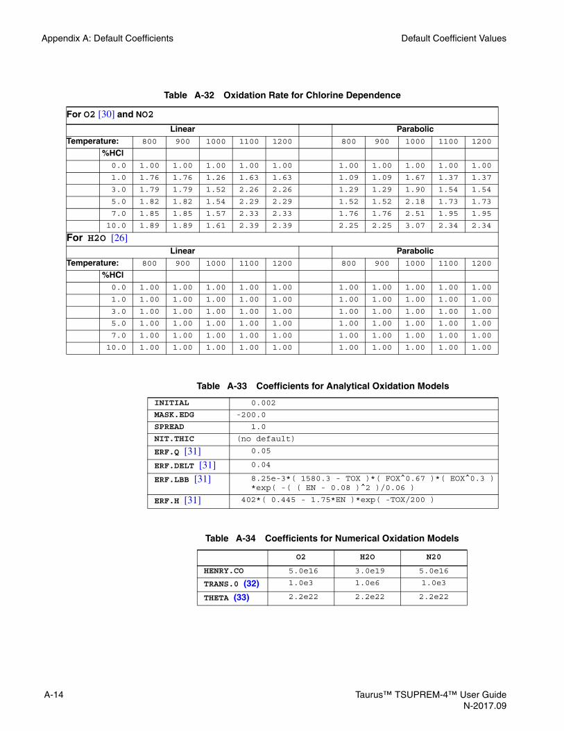
Appendix A: Default Coefficients Default Coefficient Values

Table A-32 Oxidation Rate for Chlorine Dependence

For O2 [30] and NO2

Linear ParabolicTemperature: 800 900 1000 1100 1200 800 900 1000 1100 1200

%HCl00.0 1.00 1.00 1.00 1.00 1.00 1.00 1.00 1.00 1.00 1.00

01.0 1.76 1.76 1.26 1.63 1.63 1.09 1.09 1.67 1.37 1.37

03.0 1.79 1.79 1.52 2.26 2.26 1.29 1.29 1.90 1.54 1.54

05.0 1.82 1.82 1.54 2.29 2.29 1.52 1.52 2.18 1.73 1.73

07.0 1.85 1.85 1.57 2.33 2.33 1.76 1.76 2.51 1.95 1.95

10.0 1.89 1.89 1.61 2.39 2.39 2.25 2.25 3.07 2.34 2.34

For H2O [26]Linear Parabolic

Temperature: 800 900 1000 1100 1200 800 900 1000 1100 1200

%HCl00.0 1.00 1.00 1.00 1.00 1.00 1.00 1.00 1.00 1.00 1.00

01.0 1.00 1.00 1.00 1.00 1.00 1.00 1.00 1.00 1.00 1.00

03.0 1.00 1.00 1.00 1.00 1.00 1.00 1.00 1.00 1.00 1.00

05.0 1.00 1.00 1.00 1.00 1.00 1.00 1.00 1.00 1.00 1.00

07.0 1.00 1.00 1.00 1.00 1.00 1.00 1.00 1.00 1.00 1.00

10.0 1.00 1.00 1.00 1.00 1.00 1.00 1.00 1.00 1.00 1.00

Table A-33 Coefficients for Analytical Oxidation Models

INITIAL 0000.002

MASK.EDG -200.0

SPREAD 001.0

NIT.THIC (no default)

ERF.Q [31] 0000.05

ERF.DELT [31] 0000.04

ERF.LBB [31] 00 8.25e-3*( 1580.3 - TOX )*( FOX^0.67 )*( EOX^0.3 )*exp( -( ( EN - 0.08 )^2 )/0.06 )

ERF.H [31] 402*( 0.445 - 1.75*EN )*exp( -TOX/200 )

Table A-34 Coefficients for Numerical Oxidation Models

O2 H2O N20

HENRY.CO 05.0e16 03.0e19 5.0e16

TRANS.0 (32) 1.0e3 1.0e6 1.0e3

THETA (33) 02.2e22 02.2e22 2.2e22

A-14 Taurus™ TSUPREM-4™ User GuideN-2017.09

Default Coefficient Values Appendix A: Default Coefficients

Table A-35 Diffusivity of Oxidizing Species in Ambient (7)

O2 H2O N20

D.0 03.5e9 002.5e7 3.5e9

D.E 1.25 0.8 1.25

Table A-36 Nitrogen-dependent Oxide Growth Coefficients (cm.s)

O2 H2O N20

Oxide/Silicon, Oxide/Polysilicon

N.G.0 0.0 0.0 5.2e22

N.G.E 0.0 0.0 0.0

N.V.0 0.0 0.0 1.0

N.V.E 0.0 0.0 0.0

N.GPOW.0 0.0 0.0 0.0

N.GPOW.E 0.0 0.0 0.0

N.THIN.0

<111> 0.0 0.0 1.55e14

<110> 0.0 0.0 1.55e14

<100> 0.0 0.0 1.55e14

N.THIN.E

<111> 0.0 0.0 0.0

<110> 0.0 0.0 0.0

<100> 0.0 0.0 0.0

Table A-37 Parameters for Stress-Dependent Oxidation

STRESS.D true

VC 300.0 (oxide), 130.0 (nitride) (34)VR 015 [42]VD 075.0 [42]VT 000.0

VDLIM 001.2

Table A-38 Material Conversion Coefficient

ALPHA

Silicon/oxide 0.44 [49]Polysilicon/oxide 0.44 (38)Other pairs of materials 1.000000

Taurus™ TSUPREM-4™ User Guide A-15N-2017.09

Appendix A: Default Coefficients Default Coefficient Values

Diffusion Enhancement in Oxides

Silicidation

Table A-39 Diffusion Enhancement Factor of Boron in Oxides

1+4.55e-22*exp(0.28/kt)*sio+2.23e-20*fluorine

Table A-40 Diffusivity of Silicon in Oxides (CM.SEC units)

D.0 13.0

D.E 04.5

Table A-41 Si and SiO Reactions in Oxides

MAT.BULK oxide oxide

/MAT.L oxide oxide

/NM.L 0 0 0

MAT.R silicon ambient

NM.R 0 0

IMP.L iox sio

NI.L 1.0 1.0

EI.L 1.00 1.0

/IMP.L O2 O2 iox iox

/NI.L 0.0 0.0 1.0 1.0

/EI.L 0.5 0.5 1.0 1.0

IMP.R sio interst O2

NI.R 1.0 1.0 0

EI.R 1.00 1.0 1.0

RATE.0 7.673e6 7.673e6 0.01 8.67e7

RATE.E 4.00 4.00 0.0 4.00

EQUIL.0 0 0 2.95e-5 0

EQUIL.E 00 00 -2.19 0

Table A-42 Diffusivity of Silicon in Silicides (CM.SEC units)

TiSi2 (35) [32] WSi2 (36) [33]-[35] CoSi2 NiSi2

D.0 2.0 006.86e3 5.0 5.0

D.E 01.86 2.72 02.30 2.30

Table A-43 Diffusivity of ORSoxygen in Silicides (CM.SEC units)

TiSi2 WSi2 CoSi2 NiSi2D.0 15. 15. 15. 15.

D.E 2.56 2.56 2.56 2.56

A-16 Taurus™ TSUPREM-4™ User GuideN-2017.09

Default Coefficient Values Appendix A: Default Coefficients

Table A-44 Titanium Silicidation Reactions

/MAT.L TiSi2 TiSi2 titanium TiSi2

/NM.L 00 00 0.5 00

MAT.R silicon polysilicon TiSi2 oxide

NM.R 1.0 1.0 0.5 0

IMP.L vacancy silicon

NI.L 1.0e-3 1.0

EI.L 00 1.0

/IMP.L silicon silicon ORSoxygen

/NI.L 1.0 1.0 1.0

/EI.L 1.0 1.0 1.0

RATE.0 1.0e-3 1.0e-3 104.0 1.667e-4

RATE.E 00 00 1.0 00

EQUIL.0 1.0e20 1.0e20 1.0 1.0e22

EQUIL.E 00 00 0 00

R.FAC max((1-ORSoxygen/1e22),0.) 10

Table A-45 Tungsten Silicidation Reactions [33]-[35]

/MAT.L WSi2 WSi2 tungsten WSi2

/NM.L 000 000 0.5 00

MAT.R silicon polysilicon WSi2 oxide

NM.R 1.0 1.0 0.5 0

IMP.L vacancy silicon

NI.L 1.0e-3 1.0

EI.L 000 1.0

/IMP.L silicon silicon ORSoxygen

/NI.L 1.0 1.0 1.0

/EI.L 1.0 1.0 1.0

RATE.0 1.0e-1 1.0e-1 4.60e3 (37) 1.667e-4

RATE.E 000 000 1.64 (37) 00

EQUIL.0 1.0e20 1.0e20 1.00 1.0e22

EQUIL.E 000 000 000 00

R.FAC max((1-ORSoxygen/1e22),0.) 10

Table A-46 Cobalt Silicidation Reactions

/MAT.L CoSi2 CoSi2 Cobalt CoSi2

/NM.L 00 00 0.5 00

MAT.R silicon polysilicon CoSi2 oxide

NM.R 1.0 1.0 0.5 0

IMP.L silicon

NI.L 1.0

EI.L 1.0

/IMP.L silicon silicon ORSoxygen

/NI.L 1.0 1.0 1.0

Taurus™ TSUPREM-4™ User Guide A-17N-2017.09

Appendix A: Default Coefficients Default Coefficient Values

Analytical Implant

/EI.L 1.0 1.0 1.0

RATE.0 1.667e-4 1.667e-4 1.0e4 1.667e-4

RATE.E 00 00 1.84 00

EQUIL.0 2.34e22 2.34e22 1.0 3.0e21

EQUIL.E 00 00 0 00R.FAC max((1-ORSoxygen/1e22),0.) 10

Table A-46 Cobalt Silicidation Reactions (Continued)

Table A-47 Nickel Silicidation Reactions

/MAT.L NiSi2 NiSi2 Nickel NiSi2

/NM.L 00 00 0.5 00

MAT.R silicon polysilicon NiSi2 oxide

NM.R 1.0 1.0 0.5 0

IMP.L silicon

NI.L 1.0

EI.L 1.0

/IMP.L silicon silicon ORSoxygen

/NI.L 1.0 1.0 1.0

/EI.L 1.0 1.0 1.0

RATE.0 1.667e-4 1.667e-4 1.0e4 1.667e-4

RATE.E 00 00 1.84 00

EQUIL.0 2.34e22 2.34e22 1.0 1.0e22

EQUIL.E 00 00 0 00

R.FAC max((1-ORSoxygen/1e22),0.) 10

Table A-48 Effective +n Model (in Silicon)

D.PHDF 0.0905

D.PME 0.85

D.PLF -2

D.PLME -0.5

D.PCONST 3.25

D.PDME -0.5

D.PDLF -2

D.PDLME -0.5

D.PNORM 3e12

D.PDE 1

D.PRE 0

D.PFACTO 0

A-18 Taurus™ TSUPREM-4™ User GuideN-2017.09

Default Coefficient Values Appendix A: Default Coefficients

Taurus MC Implant

Table A-49 Taurus Analytic Implant Model Parameters

Boron Phosphorus Indium Antimony Fluorine Nitrogen Silicon Aluminum Others

All materialsRANGE.F 6.0 5.0 3.0 3.0 6.0 6.0 5.0 5.5 4.0

SIGMA.F 6.0 5.0 3.0 3.0 6.0 6.0 5.0 5.5 4.0

D.RAN.F 0.6 5.0 3.0 3.0 3.0 1.0 5.0 4.0 4.0

D.SIG.F 6.0 5.0 3.0 3.0 6.0 6.0 5.0 5.5 4.0

D.SUP.R 0.01 0.01 0.01 0.01 0.01 0.01 0.01 0.01 0.01

D.SUP.E 0.4 0.4 0.2 0.2 0.4 0.4 0.4 0.4 0.4

Table A-50 Ge-Dependent Reshaping Model Parameters

Boron Arsenic Other impurities

SiliconRANGE.0 0.266 0.617 0.0

RANGE.F 7.68 1.05 0.0

SIGMA.0 0.343 0.547 0.0

SIGMA.F 3.67 0.437 0.0

D.RAN.0 0.302 0.00783 0.0

D.RAN.F 1.75 0.606 0.0

D.SIG.0 0.207 0.477 0.0

D.SIG.F 1.55 6.76 0.0

D.SUP.R 0.1 0.01 0.0

D.SUP.E 0.0 0.4 0.0

Table A-51 Electronic Stopping Power (LSS Correction Factor: LSS.PRE)

Boron Fluorine Phosphorus Germanium Indium Arsenic AntimonySilicon 1.5 1.1 1.25 1.0 1.0 1.0 1.0

Polysilicon 1.5 1.1 1.25 1.0 1.0 1.0 1.0

Oxide 1.04 1.0 1.0 1.0 1.0 1.0 1.0

Nitride 1.1 1.0 0.85 1.0 1.0 1.0 1.0

SiC 1.35 1.0 0.95 1.0 1.0 1.0 1.0

Other 1.0 1.0 1.0 1.0 1.0 1.016 1.0.5

Table A-52 Electronic Stopping Power Model (Silicon)

Boron Fluorine Phosphorus Germanium Indium Arsenic Antimony

LSS.PRE 1.5 1.1 1.25 1.0 1.0 1.0 1.0

NLOC.PRE 0.44 0.15 0.44 0.44 0.44 0.35 0.44

NLOC.EXP 0.075 0.075 0.075 0.075 0.075 0.075 0.075

SCR.PAR 1.0 1.0 1.0 1.0 1.0 1.0 1.0

Taurus™ TSUPREM-4™ User Guide A-19N-2017.09

Appendix A: Default Coefficients Default Coefficient Values

Electrical Parameters

Table A-53 Damage Accumulation and Dechanneling Model (Silicon)

Boron Fluorine Phosphorus Germanium Indium Arsenic Antimony

SURV.RAT 0.225 0.5 0.75 0.9 1.5 0.9 1.8

CASC.SUR 0.225 0.5 0.75 0.9 1.5 0.9 1.8

DISP.THR 15.0 15.0 15.0 15.0 10.0 15.0 15.0

CASC.DIS 15.0 15.0 15.0 15.0 10.0 15.0 15.0

AMOR.PAR 1.0 1.0 1.0 1.0 1.0 1.0 1.0

CASC.AMO 1.0 1.0 1.0 1.0 1.0 1.0 1.0

Table A-54 Critical Electric Field (volts/cm) [36] [37]

ECN.MU 6.49e4

ECP.MU 1.87e4

Table A-55 Surface Mobility Degradation Factor

GSURFN 1.0

GSURFP 1.0

Table A-56 Arora Mobility Model [38]

MUN1 88.00

MUN2 1252.0000

AN 0 0.88

CN 0001.26e17

EXN1 0-0.570

EXN2 0 -2.330

EXN3 0 2.40

EXN4 -0.146

MUP1 0 54.30

MUP2 407.00

AP 00 0.88

CP 0002.35e17

EXP1 00-0.57

EXP2 00-2.23

EXP3 00 2.4

EXP4 -0.146

A-20 Taurus™ TSUPREM-4™ User GuideN-2017.09

Default Coefficient Values Appendix A: Default Coefficients

Table A-57 Caughey Mobility Model [39]

MUN.MIN 55.24

MUN.MAX 1429.2300

NREFN 0001.072e17

NUN -2.30

XIN -3.80

ALPHAN 0 0.733

MUP.MIN 049.705

MUP.MAX 479.370

NREFP 0001.606e17

NUP -2.20

XIP -3.70

ALPHAP 00.70

Table A-58 Mobility Table

Concentration Mobility at 300 K

(#/cm3) Electron Hole

1e14 1350 495

2e14 1345 495

4e14 1335 495

6e14 1320 495

8e14 1310 495

1e15 1300 491.1

2e15 1248 487.3

4e15 1200 480.1

6e15 1156 473.3

8e15 1115 466.9

1e16 1076 460.9

2e16 960 434.8

4e16 845 396.5

6e16 760 369.2

8e16 720 348.3

1e17 675 331.5

2e17 524 279.0

4e17 385 229.8

6e17 321 203.8

8e17 279 186.9

1e18 252 178.0

2e18 182.5 130.0

4e18 140.6 90.0

6e18 113.6 74.5

8e18 99.5 66.6

1e19 90.5 61.0

2e19 86.9 55.0

4e19 83.4 53.7

Taurus™ TSUPREM-4™ User Guide A-21N-2017.09

Appendix A: Default Coefficients Default Coefficient Values

Material Coefficients

6e19 78.8 52.9

8e19 71.6 52.4

1e20 67.8 52.0

2e20 52.0 50.8

4e20 35.5 49.6

6e20 23.6 48.9

8e20 19.0 48.4

1e21 17.8 48.0

Table A-58 Mobility Table (Continued)

Concentration Mobility at 300 K

Table A-59 Semiconductor Material Coefficients

Silicon Polysilicon (38) SiC (39)

DENSITY 2.330000000 2.33000000 3.21

AT.NUM 14.0000000000 14.00000000 10.0

AT.WT 28.0690000000 28.0690000000 20.04

AT.RAD 1.17 (angstroms)00

00000000

MOL.WT 28.0690000000 28.0690000000 40.08

POLYCRYS false true

NI.0 3.87e16 [40] 3.87e1600

NI.E 0.605000000 0.60500000

NI.F 1.500000000 1.50000000

YOUNG.M 1.87e12 [42] 1.87e12 [42]POISS.R 0.280000000 0.280000000

C11.0 16.57e11 0

C11.1 -1.347e80000000 00000000

C12.0 6.331e11 0

C12.1 -0.538e80000000 00000000

C44.0 8.022e11 0

C44.1 -0.607e80000000 00000000

VISC.0 1.0e30000000 1.0e1600000

VISC.E 0.000000000 0.000000000

VISC.X 0.499000000 0.499000000

EPSILON 11.7 [42]0000 11.7000000000

E.FIELD true true

AFFINITY 4.1700000000 4.170000000

BANDGAP 1.0800000000 1.080000000

EGALPH 4.73e-4 4.73e-4

EGBETA 636 636

N.CONDUC 2.82e1900000 2.82e190000

N.VALENC 1.04e1900000 1.04e190000

NC.F 1.5 1.5

A-22 Taurus™ TSUPREM-4™ User GuideN-2017.09

Default Coefficient Values Appendix A: Default Coefficients

NV.F 1.5 1.5

G.DONOR 2.0000000000 2.000000000

E.DONOR 0.0490000000 0.049000000

G.ACCEP 4.0000 4.00000

E.ACCEP 0.0450 0.04500

BOLTZMAN false false

IONIZATI true true

QM.BETA 4.1e-8 4.1e-80

QM.YCRIT 25e-8 25e-8

TIF.NAME Si Poly SiC

MD.INDEX 100000 3000000 8

ION.PAIR true true

IP.OMEGA 6.000 6.0000

CL.MODEL true

MAX.DAMA 1.15e22

DAM.GRAD 10

D.PCONST 0.42

EQACT.IN true true

Table A-60 Polycrystalline Material Coefficients (40)

Polysilicon

F11 1.0

F22 2.0

G.DENS 2.0

GRASZ.0 0.1

GRASZ.E 0.0

TEMP.BRE 600.000

MIN.GRAI 0.005

FRAC.TA 0.5

GEOM 6.0

GAMMA.0 0005.6e-6

GAMMA.E 00-1.7300

GBE.0 00000.39125

GBE.H 3.0

GBE.1 0.0

ALPHA 01.33

DSIP.0 30.00

DSIP.E 05.09

DSIX.0 000.015

DSIX.E 03.89

DSIM.0 16.00

DSIM.E 04.54

DSIMM.0 166.700

DSIMM.E 5.0

NSEG 2.0

Table A-59 Semiconductor Material Coefficients (Continued)

Silicon Polysilicon (38) SiC (39)

Taurus™ TSUPREM-4™ User Guide A-23N-2017.09

Appendix A: Default Coefficients Default Coefficient Values

TBU.0 1.0

TBU.E -5.00

TOXIDE 0000.0005

DLGX.0 000

DLGX.E 04.40

EAVEL.0 000

EAVEL.E 3.0

GB.THICK 0.0005

Table A-60 Polycrystalline Material Coefficients (40) (Continued)

Polysilicon

Table A-61 Insulator Material Coefficients

Oxide HfO2 Nitride Oxynitride Ambient

DENSITY 2.235 9.68 3.44 2.235

AT.NUM (avg) 10.0000 29.333 10.000 10.000

AT.WT (avg) 20.0230 70.163 20.030 20.023

MOL.WT 60.0690 210.488 140.2100 60.069

POLYCRYS false false false false

YOUNG.M 6.6e11 [42] 5.654e11 003.89e12 03.89e12

POISS.R 0.17 [42] 0.2 0.300 0.30

VISC.0 5.25e4 (41) 5.25e4 001.3e6 (41) 01.3e6 (41) 1.0e9 (42)VISC.E -2.42 (41) -2.42 0-2.42 (41) -2.42 (41) 0.00 (42)VISC.X 0.4990 0.499 0.499 00.499 0.30 (42)EPSILON 03.9 [43] 21 007.5 [44] 7.50 1.0000000

TIF.NAME Ox0000 HfO2 Nit OxyNit Ambient

MD.INDEX -1000000 -4 -200000 -60000 -400000000

IMPL.TAB oxide oxide nitride oxide

Table A-62 Other Material Coefficients

Aluminum Photoresist Titanium TiSi2 Tungsten WSi2

DY.DEFAU 0.0250 0.02000

DENSITY 02.7020 1.060 4.5 4.0443 19.3000000 9.85700

AT.NUM 13.00 2.875 22.00 16.67000 74.0000000 34.000000

AT.WT 26.98 5.125 47.90 34.68000 183.8500000 80.000000

MOL.WT 26.98 41.0000 47.90 104.038000 183.8500000 240.0000000

POLYCRYS false false false false

YOUNG.M 8.6e11 3.24e10 01.0e13 1.0e13 3.66e12 1.0e110

POISS.R 0.295 0.35 0.3 0.3000 0.29592 0.29592

EPSILON 1.0 1.00

WORKFUNC 4.1 04.80 4.8000 4.80000 4.80000

TIF.NAME Al Photo Ti TiSi2 W WSi2

MD.INDEX -5000 -4000 -5000 -500000 -5 -5

IMPL.TAB aluminum az-7500 titanium tisi2 tungsten wsi2

A-24 Taurus™ TSUPREM-4™ User GuideN-2017.09

Default Coefficient Values Appendix A: Default Coefficients

Numerical Methods

Table A-63 Other Material Coefficients

Cobalt CoSi2 Nickel NiSi2

DY.DEFAU 0.0250 0.025000

DENSITY 8.9 4.9 8.9100 4.9

AT.NUM 27.00 18.33000 28.0000000 18.6700000

AT.WT 58.93 38.36000 58.6900000 38.29000

MOL.WT 58.93 115.09000 58.69 114.69

POLYCRYS false false false false

YOUNG.M 01.914e12 1.6e12 1.86e12 1.146e120

POISS.R 0.322 0.25000 0.342 0.33

EPSILON

WORKFUNC 05.0 5.0000 5.0000 5.0000

TIF.NAME Co CoSi2 Ni NiSi2

MD.INDEX -5000 -500000 -5 -5

IMPL.TAB Cobalt cosi2 nickel nisi2

Table A-64 Linear Coefficients of Thermal Expansion

Silicon 3.052e-6 + 2*6.206e-10*(T -293)

Oxide 1.206e-7 + 2*2.543e-10*(T -293)

HfO2 1.31e-6

Nitride 3.0e-6

Aluminum 2.438e-5 + 2*6.660e-9*(T -293)

Cobalt 13.8e-06 + 1.332e-8*(T -293)

CoSi2 10.8e-6 + 1.332e-8*(T -293)

Nickel 1.25e-5

Tungsten 4.6e-6

WSi2 8.21e-6

SiC 4.8e-6

Oxynitride 3.0e-6

Photores 5.5e-5

Other materials 0.0

Table A-65 Block Solution Parameters

Impurities Point Defects Oxidant TrapsREL.ERR 0.01 0.01 0.01 0.01

ABS.ERR 01.0e9 01.0e5 01.0e9 01.0e9

Factoring TIME.STE TIME.STE TIME.STE TIME.STE

SYMMETRY false false false false

Fill PART FULL PART NONE

Block solve LU LU LU LU

Taurus™ TSUPREM-4™ User Guide A-25N-2017.09

Appendix A: Default Coefficients Default Coefficient Values

Automatic Grid Generation Parameters

Table A-66 System Solution Parameters

MIN.FILL true

MIN.FREQ 1.100

MF.METH 1

MF.DIST 0.5

System solve CG

BACK 18

BLK.ITLI 20

Integration TRBDF

INIT.TIM 0.002

Table A-67 Models

Oxidation VERTICAL

Point defect PD.FERMI

Bulk recombination KB.LOW

SKIP.SIL true

OX.REL 1.0e-6

CONTIN.M 2

VE.SMOOT 0.0400

V.COMPAT current version

Table A-68 Program Options

INFORMAT false

DIAGNOST false

ECHO true

EXECUTE true

Output NORMAL

Table A-69 Automatic Grid Generation Parameters

DX.MIN 0.2

DX.MAX 0.5

DX.RATIO 1.5

DY.SURF 00.05 LY.SURF 0.1

DY.ACTIV 0.5 LY.ACTIV 4.0

DY.BOT 100.000 LY.BOT 200.000

DY.RATIO 1.5

A-26 Taurus™ TSUPREM-4™ User GuideN-2017.09

Default Coefficient Values Appendix A: Default Coefficients

Adaptive Grid Parameters

Table A-70 Global Grid Spacing Factors

GRID.FAC 1.0

DY.OXIDE 0.1

DY.EXACT true

DY.LOCAL true

Table A-71 Dopants

For Antimony, Arsenic, Boron, Indium, and PhosphorusSilicon Polysilicon Oxide Other (46)

REL.ADAP 0.200 0.30 2.00 0.0

ABS.ADAP 01.0e14 001.0e15 001.0e16 0.0

MIN.SPAC 0.025 0.03 0.10 0.0

Table A-72 Silicon in TiSi2, WSi2, CoSi2, and NiSi2

REL.ADAP 0.100

ABS.ADAP 01.0e15

MIN.SPAC 0.010

Table A-73 O2 and H2O in Oxide

O2 H2O

REL.ADAP 0.20 0.20

ABS.ADAP 1.0e14 1.0e17

MIN.SPAC 0.01 0.01

Table A-74 Unrefinement Parameters

Silicon Other (46)MAX.SPAC 0.2500 0.0

Table A-75 Control Parameters

IMP.ADAP true

DIF.ADAP true

OX.ADAPT true

ERR.FAC 1.0

ERR.INIT 1e-5

UNREFINE 0.25

Taurus™ TSUPREM-4™ User Guide A-27N-2017.09

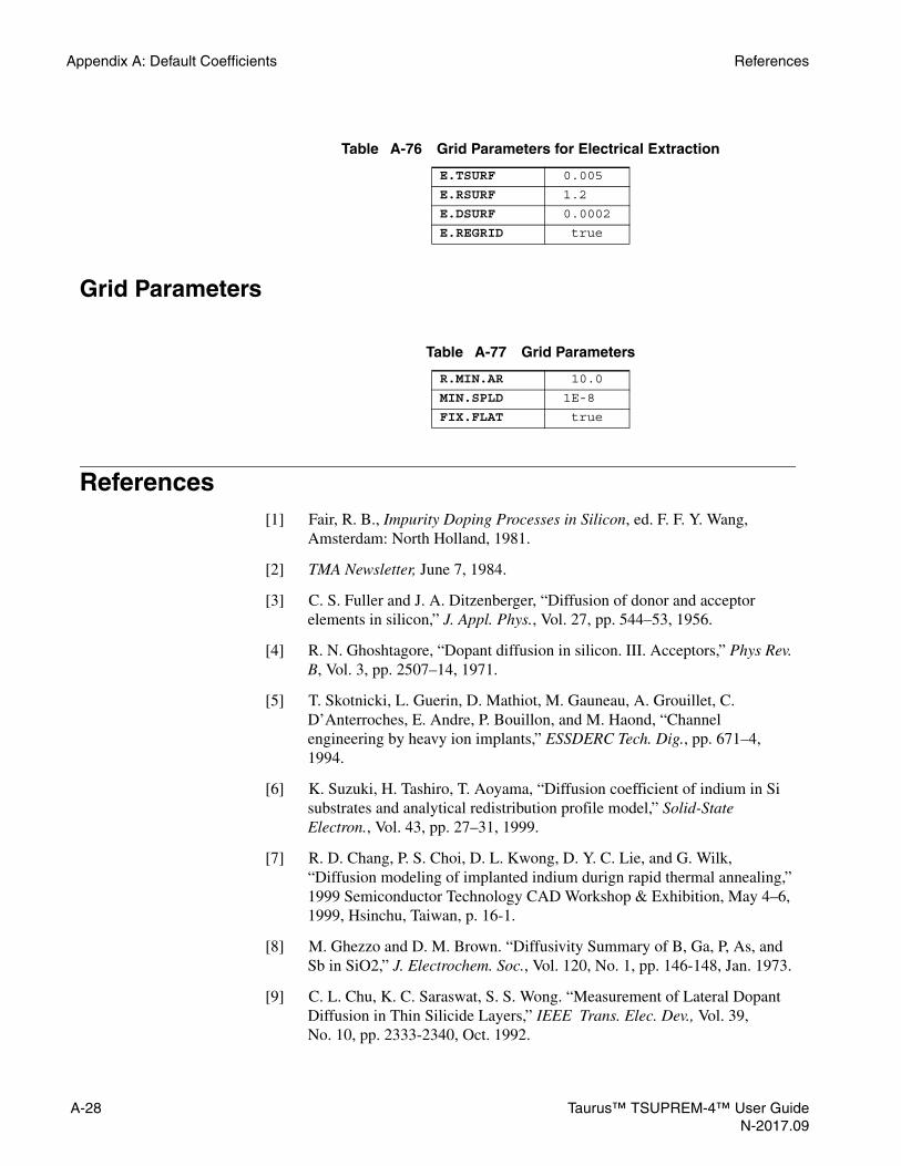
Appendix A: Default Coefficients References

Grid Parameters

References[1] Fair, R. B., Impurity Doping Processes in Silicon, ed. F. F. Y. Wang,

Amsterdam: North Holland, 1981.

[2] TMA Newsletter, June 7, 1984.

[3] C. S. Fuller and J. A. Ditzenberger, “Diffusion of donor and acceptor elements in silicon,” J. Appl. Phys., Vol. 27, pp. 544–53, 1956.

[4] R. N. Ghoshtagore, “Dopant diffusion in silicon. III. Acceptors,” Phys Rev. B, Vol. 3, pp. 2507–14, 1971.

[5] T. Skotnicki, L. Guerin, D. Mathiot, M. Gauneau, A. Grouillet, C. D’Anterroches, E. Andre, P. Bouillon, and M. Haond, “Channel engineering by heavy ion implants,” ESSDERC Tech. Dig., pp. 671–4, 1994.

[6] K. Suzuki, H. Tashiro, T. Aoyama, “Diffusion coefficient of indium in Si substrates and analytical redistribution profile model,” Solid-State Electron., Vol. 43, pp. 27–31, 1999.

[7] R. D. Chang, P. S. Choi, D. L. Kwong, D. Y. C. Lie, and G. Wilk, “Diffusion modeling of implanted indium durign rapid thermal annealing,” 1999 Semiconductor Technology CAD Workshop & Exhibition, May 4–6, 1999, Hsinchu, Taiwan, p. 16-1.

[8] M. Ghezzo and D. M. Brown. “Diffusivity Summary of B, Ga, P, As, and Sb in SiO2,” J. Electrochem. Soc., Vol. 120, No. 1, pp. 146-148, Jan. 1973.

[9] C. L. Chu, K. C. Saraswat, S. S. Wong. “Measurement of Lateral Dopant Diffusion in Thin Silicide Layers,” IEEE Trans. Elec. Dev., Vol. 39, No. 10, pp. 2333-2340, Oct. 1992.

Table A-76 Grid Parameters for Electrical Extraction

E.TSURF 0.0050

E.RSURF 1.2000

E.DSURF 0.0002

E.REGRID true

Table A-77 Grid Parameters

R.MIN.AR 10.0

MIN.SPLD 1E-800

FIX.FLAT true

A-28 Taurus™ TSUPREM-4™ User GuideN-2017.09

References Appendix A: Default Coefficients

[10] V. Probst, H. Schaber, A. Mitwalsky, and H. Kabza. “WSi2 and CoSi2 as Diffusion Sources for Shallow-Junction Formation in Silicon,” J. Appl. Phys., Vol. 70, No. 2, pp. 708-719, July 1991.

[11] M. Y. Tsai, F. M. d’Heurle, C. S. Petersson, and R. W. Johnson. “Properties of Tungsten Silicide Film on Polycrystalline Silicon,” J. Appl. Phys., Vol. 52, No. 8, pp. 5350-5355, Aug. 1981.

[12] G. Giroult, A. Nouailhat, and M. Gauneau.“Study of a WSi2/Polycrystalline Silicon/Monocrystalline Silicon Structure for a Complementary Metal-Oxide-Semiconductor for a Compatible Self-Aligned Bipolar Transistor Emitter,” J. Appl. Phys., Vol. 67, No. 1, pp. 515-523, Jan. 1990.

[13] D. A. Antoniadis, A. G. Gonzalez, and R. W. Dutton. “Boron in Near-Intrinsic <100> and <111> Silicon under Inert and Oxidizing Ambients—Diffusion and Segregation,” J. Electrochem. Soc., Vol. 125, No. 5, pp. 813-819, May 1978.

[14] H. F. Wolf. Semiconductors, Interscience, p. 361, 1971.

[15] I. C. Kizilyalli, T. L. Rich, F. A. Stevie, and C. S. Rafferty, “Diffusion parameters of indium for silicon process modeling,” J. Appl. Phys., Vol. 80, no. 9, pp. 4944–7, 1 Nov 1996.

[16] P. H. Langer and J. I. Goldstein.“Boron Autodoping During Silane Epitaxy,” J. Electrochem. Soc., Vol. 124, No. 4, pp. 591-598, April 1977.

[17] F. Lau, L. Mader, C. Mazure, C. Werner, and M. Orlowski. “A Model for Phosphorus Segregation at the Silicon-Silicon Dioxide Interface,” Appl. Phys. A., 49, pp. 671-675, 1989.

[18] H. Vuong, C. Rafferty, S. Eshraghi, J. Lentz, P. Zeitzoff, M. Pinto, and S. Hillenius, “Effects of Oxide Interface Traps and Transient Enhanced Diffusion on the Process Modeling of PMOS Devices,” IEEE Trans. Electron Devices, Vol. ED-43, No. 7, pp. 1144-1152, July 1996.

[19] G. L. Vick and K. M. Whittle. “Solid Solubility and Diffusion Coefficients of Boron in Silicon,” J. Electrochem. Soc., Vol. 116, No. 8, pp. 1142-1144, Aug. 1969.

[20] F. A. Trumbore. “Solid Solubilities of Impurity Elements in Germanium and Silicon,” Bell System Tech. J., Vol. 39, pp. 205-233, Jan. 1960.

[21] M. R. Kump. “2-D Computer Simulation of Diffusion in Silicon,” Doctoral Dissertation, Stanford University, Stanford, California, March 1988.

[22] S. T. Dunham. J. Appl. Phys., Vol. 71, No. 1, 1992.

[23] J. M. Poate, D. J. Eaglesham, G. H. Gilmer, H. J. Gossmann, M. Jaraiz, C. S. Rafferty, and P. A. Stolk. “Ion Implantation and Transient Enhanced Diffusion,” 1995 IEDM Tech. Dig., pp. 77-80, 1995.

Taurus™ TSUPREM-4™ User Guide A-29N-2017.09

Appendix A: Default Coefficients References

[24] R. Y. S Huang and R. W. Dutton. “Experimental Investigation and Modeling of the Role of Extended Defects During Thermal Oxidation,” J. Appl. Phys., Vol. 74, No. 9, pp. 5821-5827, Nov. 1993.

[25] S. M. Hu. Defects in Semiconductors, ed. J. Narayan and T. Y. Tan, Amsterdam: North-Holland, pp. 333-354, 1981.

[26] Deal, B. E., “Thermal Oxidation Kinetics of Silicon in Pyrogenic H2O and 5% HC1/H2O Mixtures,” J. Electrochem. Soc., Vol. 125, No. 4, pp. 576-579, Apr 1978.

[27] R. R. Razouk, L. N. Lie, and B. E. Deal. “Kinetics of High Pressure Oxidation of Silicon in Pyrogenic Steam,” J. Electrochem. Soc., Vol. 128, No. 10, pp. 2214-2220, Oct. 1981.

[28] C. P. Ho and J. D. Plummer. “Si/SiO2 Interface Oxidation Kinetics: A Physical Model for the Influence of High Substrate Doping Levels,” J. Electrochem. Soc., Vol. 126, No. 9, pp. 1516-1522, Sept. 1979.

[29] H. Z. Massoud. “Thermal Oxidation of Silicon in Dry Oxygen—Growth Kinetics and Charge Characterization in the Thin Regime,” Technical Report, Stanford Electronics Laboratories, Stanford University, Stanford, California, June 1983.

[30] D. W. Hess and B. E. Deal. “Kinetics of the Thermal Oxidation of Silicon in O2/HCl Mixtures,” J. Electrochem. Soc., Vol. 124, No. 5, pp. 735-739.

[31] N. Guillemot, G. Pananakakis, and P. Chenevier. “A New Analytical Model of the ‘Bird’s Beak’,” IEEE Trans. Electron Devices, Vol. ED-34, No. 7, pp. 744-749, July 1983.

[32] L. S. Hung, et al. J. Appl. Phys., Vol. 54 p. 5076, 1983.

[33] S. L. Zhang, R. Buchta, and M. Ostling. “A Study of Silicide Formation form LPCVD-Tungsten Films: Film Texture and Growth Kinetics,” J. Mater. Res., Vol. 6, pp. 1886-1891, Sept. 1991.

[34] L. D. Locker and C. D. Capio. “Reaction Kinetics of Tungsten Thin Films on Silicon (100) Surfaces,” J. Appl. Phys., Vol. 44, No. 10, pp. 4366-4369, Oct. 1973.

[35] E. Ma, B. S. Lim, M. A. Nicolet, N. S Alvi, and A. H. Hamdi. J. Electron. Mater., Vol. 17, p. 207, 1988.

[36] K. Yamaguchi.“Field-dependent Mobility Model for 2-D Numerical Analysis of MOSFETs,” IEEE Trans. Electron Devices, Vol. ED-26, pp. 1068-1074, July 1979.

[37] K. Yamaguchi. “A Mobility Model for Carriers in the MOS Inversion Layer,” IEEE Trans. Electron Devices, Vol. ED-30, pp. 658-663, June 1983.

[38] N. D. Arora, J. R. Hauser, and D. J. Roulston. “Electron and Hole Mobilities in Silicon as a Function of Concentration and Temperature,” IEEE Trans. Electron Devices, Vol. ED-29, pp. 292-295, Feb. 1982.

A-30 Taurus™ TSUPREM-4™ User GuideN-2017.09

References Appendix A: Default Coefficients

[39] D. M. Caughey and R. E. Thomas. “Carrier Mobilities in Silicon Empirically Related to Doping and Field,” Proc. IEEE, Vol. 55, pp. 2192-2193, 1967.

[40] F. J. Morin and J. P. Maita. “Electrical Properties of Silicon Containing Arsenic and Boron,” Phys. Rev., Vol. 96, No. 1, pp. 28-35, Oct. 1954.

[41] A. S. Grove. Physics and Technology of Semiconductor Devices, New York: John Wiley and Sons, pp. 102-103, 1967.

[42] V. Senez, P. Ferreira, and B. Baccus. “2-D Simulation of Local Oxidation of Silicon: Calibrated Viscoelastic Flow Analysis,” IEEE Trans. Electron Dev., Vol. 43, No. 5, pp. 720–731, May 1996.

[43] Handbook of Chemistry and Physics, 53rd Edition, Cleveland: The Chemical Rubber Company, 1972.

[44] R. S. Muller, and T. I. Kamins. Device Electronics for Integrated Circuits, New York: John Wiley and Sons, 1977.

[45] J. P. Biersack and L. G. Haggmark. “A Monte Carlo Computer Program for the Transport of Energetic Ions in Amorphous Targets,” Nucl. Instr. and Meth., Vol. 174, p. 257, 1980.

[46] R. G. Wilson. “Random and Channeled Implantation Profiles and Range Parameters for P and Al in Crystalline and Amorphized Si,” J. Appl. Phys., Vol. 59, p. 2797-2805, Oct. 1986.

[47] J. Comas and R. G. Wilson. “Channeled and Random Equivalent Depth Distributions of 150keV Li, Be, and B Implanted in Si,” J. Appl. Phys., Vol. 51, No. 7, pp. 3697-3701, July 1980.

[48] R. G. Wilson. “Channeling of 20-800 keV Arsenic Ions in the <110> and the <100> Directions of Silicon, and the Roles of Electronic and Nuclear Stopping,” J. Appl. Phys., Vol. 52, No. 6, pp. 3985-3988, June 1981.

[49] E. Bassous, H. N. Yu, and V. Maniscalco. “Topology of Silicon Structure with Recessed SiO2,” J. Electrochem. Soc., Vol. 123, No. 11, pp. 1729-1737, Nov. 1976.

[50] T. I. Kamins and E. L. MacKenna. “Thermal Oxidation of Polycrystalline Silicon Films,” Metallurgical Transactions, Vol. 2, pp. 2292-2294, Aug. 1971.

[51] P. Fahey, G. Barbuscia, M. Moslehi, and R. W. Dutton, “Kinetics of Thermal Nitridation Processes in the Study of Dopant Diffusion Mechanisms in Silicon,” Appl Phys. Lett., Vol. 46, No. 8, p. 784, April 1985.

[52] T. E. Seidel, et al. “Rapid Thermal Annealing is Si,” Mat. Res. Symp. Proc., Vol. 35, p. 329, 1985.

[53] A. D. Buonaquisti, W. Carter, and P. H. Holloway. Thin Solid Films, Switzerland, Vol. 100, p. 235, 1983.

Taurus™ TSUPREM-4™ User Guide A-31N-2017.09

Appendix A: Default Coefficients Notes

[54] T. Kamins, et al. J. Appl. Phys., Vol. 43, p. 83, 1972.

[55] K. Sakamoto, K. Nishi, T. Yamaji, T. Miyoshi, and S. Ushio. J. Electrochem. Soc., Vol. 132, p. 2457, 1985.

[56] W. Rausch, R. Lever, and R. Kastl. J. Appl. Phys., Vol. 54, No. 8, p. 4405, 1983.

[57] H. Schaber, R. Criegern, and I. Weitzel. J. Appl. Phys, Vol. 58, No. 11, p. 4036, 1985.

[58] M. M. Mandurah, K. C. Saraswat, R. W. Dutton, and T. I. Kamins. “Dopant Segregation in Polysilicon,” J. Appl. Phys., Vol. 51, p. 5755, 1981.

[59] M. J. van Dort, et al. IEDM Tech. Digest, p. 865, 1994.

[60] P. B. Griffin. “Physics and Modeling of 2-D Diffusion in SUPREM-IV,” Doctoral Dissertation, Stanford University, Palo Alto, California, Dec. 1989.

[61] A. G. O’Neill, C. Hill, J. King, and C. Please. “A New Model for the Diffusion of Arsenic in Polycrystalline Silicon,” J. Appl. Phys., Vol. 64, No. 1, p. 167, 1988.

[62] C. Hill and S. Jones. “Growth and Microcrystalline Structure of Poly-Si,” Properties of Silicon: EMIS Data Review, No. 4, Inspec., p. 933, 1988.

[63] C. P. Ho, J. D. Plummer, S. E. Hansen, and R. W. Dutton. “VLSI Process Modeling—SUPREM III,” IEEE Trans. Elec. Dev., Vol. ED-30, No. 11, p. 1438, 1983.

[64] L. Mei and R. W. Dutton. “A Process Simulation Model for Multilayer Structures Involving Polycrystalline Silicon,” IEEE Trans. Elec. Dev., Vol. ED-29, No. 11, p. 1726, 1982.

[65] D. Gupth, D. R. Campbell, and P. S.Ho. Thin Films—Interdiffusion and Reaction, New York: John Wiley and Sons, p. 161, 1980.

[66] R. B. Fair. “Concentration Profiles of Diffused Dopants in Silicon,” Impurity Doping Processes in Silicon, ed. F. F. Y. Wang, Amsterdam: North Holland, 1981.

NotesThese notes appear in Default Coefficient Values, pp. A-1 through A-27.

(1) The ratio of the interstitial component to the vacancy component of diffusion in silicon has been set according to the fractional interstitialcy factors given in [51]. In materials other than silicon, the vacancy component is zero.

(2) The diffusivity of indium in silicon is taken to be an average of several reported values [3]–[6]; larger values (1.6exp(-3.5/kT)) have been reported for RTA[7].

A-32 Taurus™ TSUPREM-4™ User GuideN-2017.09

Notes Appendix A: Default Coefficients

TN

(3) Due to the wide spread in reported diffusivities in oxide, the values for phosphorus and arsenic diffusivity in oxide were taken to be an average of those reported in reference [8]. Diffusivity in oxide is reported to be very sensitive to diffusion ambient and impurity concentration, but this dependence is not well characterized and is not modeled in TSUPREM-4. In particular, diffusion from a gaseous source into oxide can result in a “melt-through” process with a much larger effective diffusivity than the value used in TSUPREM-4. The diffusivity of indium in oxide is known to be very fast; it has been approximated here as 10× the diffusivity in silicon.

(4) These values are for diffusion in the interior of a polysilicon grain. The diffusivities for boron, phosphorus, and antimony are identical to the values for single-crystal silicon. The values for arsenic are the same as for silicon but with the addition of the DIMM.0 and DIMM.E terms. These values were taken from the data of Siedel et al. [52] for bulk single-crystal silicon at high concentration.

(5) The diffusivity of boron is taken from the analysis of Buonaquisti et al. [53] of data measured by Kamins et al. [54], but the activation energy has been increased to that of single-crystal to reproduce measured values at low temperature. For phosphorus, the activation energy for single-crystal silicon is used, while the pre-exponential factor is taken to reproduce measured data at low temperature. For arsenic, the activation energy has been taken from Sakamoto et al. [55] and the pre-exponential factors have been fitted to diffusion profiles at 900°C for various implant doses. For antimony, a diffusivity of 104 times the value in single-crystal silicon has been assumed. Due to lack of data, the polycrystalline diffusion model has not been enabled for indium in polysilicon.

(6) Tungsten silicide is assumed to be present in polycrystalline form, with diffusion dominated by grain boundary effects. The diffusivity within the crystalline grains is used here, however. The diffusivity can be increased to approximate the effect of diffusion along grain boundaries, but numerical difficulties may arise if very large values are used.

(7) The diffusivity of impurities in ambient is used for calculating impurity diffusion through included voids in a structure. These values were chosen to be an approximate order of magnitude larger than the diffusivity in solid materials at normal processing temperatures.

(8) The diffusivities of pairs are estimated to be the same as the diffusivities of the corresponding point defects. Arbitrary (but physically reasonable) values have been chosen for the capture radii and barrier energies.

(9) Reported values for segregation constants of n-type impurities between silicon and silicon dioxide range between 10 and 1000. The value used here is a rough average of the reported values.

(10) Due to the absence of data for the segregation constants between polysilicon and silicon dioxide, these segregation constants were set equal to the segregation constants between silicon and silicon dioxide.

aurus™ TSUPREM-4™ User Guide A-33-2017.09

Appendix A: Default Coefficients Notes

(11) The transport of indium is known to be very fast; the value used here is computed by dividing the diffusivity (in the faster-diffusing material) by a distance of 1 angstrom.

(12) The values for transport constants between silicon and ambient are taken from the CASPER process modeling program referred to in reference [16]. The values are meant to characterize the impurity transport across a microscopically-clean silicon surface, as present during epitaxial deposition. These values may be too large if a native oxide is present on the surface of the silicon.

(13) Due to the absence of data for the transport constants between silicon dioxide and ambient and between polysilicon and ambient, these transport constants were set equal to the transport constants between silicon and ambient.

(14) The transport rate between polysilicon and silicon has been set sufficiently high, so that it is not the rate-limiting step in diffusion between the two materials. In the case where the behavior of a thin oxide diffusion barrier between the polysilicon and silicon must be modeled, the oxide layer should be explicitly included in the structure.

(15) The values for constants between silicon dioxide and silicon are extracted to fit the SIMS data for 30 KeV~70 KeV, 1E12/cm2~1E14/cm2 ion implantations followed by thermal processes for several different time conditions at 900°C~1200°C. Due to the absence of data for the constants between silicon dioxide and polysilicon, these constants were set equal to the constants between silicon dioxide and silicon.

(16) The values for constants between silicon dioxide and silicon are extracted to fit the Lau et.al. data [17] and the SIMS data for 30KeV and 40 KeV 1E14/cm2 ion implantation followed by the RTA for several different time conditions at 800°C~1000°C. The value of D.PLUS parameter on the implantation is set to 1.5 for the simulation. Due to the absence of data for the constants between silicon dioxide and polysilicon, these constants were set at the same values as the constants between silicon dioxide and silicon.

(17) The values for constants between silicon dioxide and silicon are extracted to fit the SIMS data for 20KeV 5E14/cm2 and 32KeV 1E15/cm2 ion implantations followed by the RTA for several different time conditions at 1000°C~1050°C. The value of MAX.DAM parameter on the implantation is set to 1.15E22/cm3 and the values for the clustering coefficients, CTN.0 and CTN.E are set to 5.35E-20 and -0.874, respectively. Due to the absence of data for the constants between silicon dioxide and polysilicon, these constants were set at the same values as the constants between silicon dioxide and silicon.

(18) The values for boron are appropriate for concentrations below solid solubility and are derived from the results of Rausch et al. [56] which are confirmed by Schaber et al. [57] to match measured polysilicon/silicon interfacial segregation. The values for phosphorus and arsenic are from Mandurah et al. [58], except that GSEG.0 has been reduced to match

A-34 Taurus™ TSUPREM-4™ User GuideN-2017.09

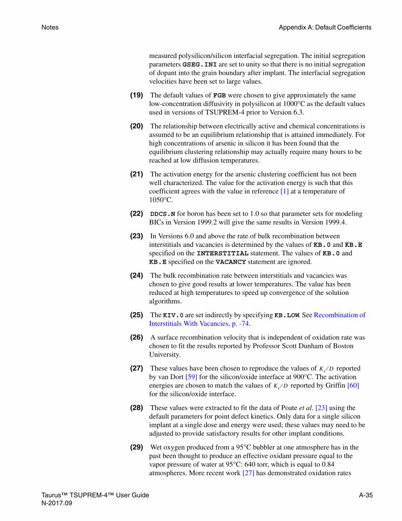
Notes Appendix A: Default Coefficients

TN

measured polysilicon/silicon interfacial segregation. The initial segregation parameters GSEG.INI are set to unity so that there is no initial segregation of dopant into the grain boundary after implant. The interfacial segregation velocities have been set to large values.

(19) The default values of FGB were chosen to give approximately the same low-concentration diffusivity in polysilicon at 1000°C as the default values used in versions of TSUPREM-4 prior to Version 6.3.

(20) The relationship between electrically active and chemical concentrations is assumed to be an equilibrium relationship that is attained immediately. For high concentrations of arsenic in silicon it has been found that the equilibrium clustering relationship may actually require many hours to be reached at low diffusion temperatures.

(21) The activation energy for the arsenic clustering coefficient has not been well characterized. The value for the activation energy is such that this coefficient agrees with the value in reference [1] at a temperature of 1050°C.

(22) DDCS.N for boron has been set to 1.0 so that parameter sets for modeling BICs in Version 1999.2 will give the same results in Version 1999.4.

(23) In Versions 6.0 and above the rate of bulk recombination between interstitials and vacancies is determined by the values of KB.0 and KB.E specified on the INTERSTITIAL statement. The values of KB.0 and KB.E specified on the VACANCY statement are ignored.

(24) The bulk recombination rate between interstitials and vacancies was chosen to give good results at lower temperatures. The value has been reduced at high temperatures to speed up convergence of the solution algorithms.

(25) The KIV.0 are set indirectly by specifying KB.LOW. See Recombination of Interstitials With Vacancies, p. -74.

(26) A surface recombination velocity that is independent of oxidation rate was chosen to fit the results reported by Professor Scott Dunham of Boston University.

(27) These values have been chosen to reproduce the values of reported by van Dort [59] for the silicon/oxide interface at 900°C. The activation energies are chosen to match the values of reported by Griffin [60] for the silicon/oxide interface.

(28) These values were extracted to fit the data of Poate et al. [23] using the default parameters for point defect kinetics. Only data for a single silicon implant at a single dose and energy were used; these values may need to be adjusted to provide satisfactory results for other implant conditions.

(29) Wet oxygen produced from a 95°C bubbler at one atmosphere has in the past been thought to produce an effective oxidant pressure equal to the vapor pressure of water at 95°C: 640 torr, which is equal to 0.84 atmospheres. More recent work [27] has demonstrated oxidation rates

Ks D⁄

Ks D⁄

aurus™ TSUPREM-4™ User Guide A-35-2017.09

Appendix A: Default Coefficients Notes

closely approximating that of a bubbler by using a pyrogenic steam process with O2 and H2 flow rates of 1.175 and 2 liters/minute, respectively. Complete reaction for these flow rates would produce an ambient containing 92% H2O and 8% O2. Because TSUPREM-4 cannot model ambients containing both H2O and O2, the wet oxygen ambient is defined as 92% H2O and 8% N2. This effective mixture of H2O and N2 will depend upon the gas flow rates, the diffusion furnace configuration, and even the altitude of the fabrication facility. As a result, these values frequently must be adjusted to achieve agreement with the oxide thicknesses grown at a particular facility.

(30) Oxidation rates for <110> silicon were not determined in references [23] and [27]. From other studies it has been found that the parabolic oxidation rates are not dependent upon the silicon orientation, but that the linear oxidation rates for <110> silicon are approximately a factor of 1.4 greater than those for <100> silicon. This factor has been used to calculate linear oxidation rates for <110> silicon from the rates for <100> silicon.

(31) The oxidation rates for polysilicon have been set equal to those for <110> silicon [50].

(32) These values are given in centimeters per second.

(33) Only one value of THETA can be given The value applies to both O2 and H2O.

(34) The default value for VC is the recommended value at 900°C. Recommended values at other temperatures are 225 at 800°C, 425 at 1000°C, and 1100 at 1100°C and higher; for nitride, use 120 at 800°C, 170 at 1000°C, and 350 at 1100°C and higher.

(35) These values are valid for reaction in argon or vacuum. Value will be smaller at high n-type concentrations.

(36) These values apply when the amount of interfacial oxygen is minimal after tungsten deposition, for example, after chemical vapor deposition. If there is significant interfacial oxygen between the tungsten and the silicon (for example, after deposition by sputtering or evaporation), the values DIX.0=9.89e4 and DIX.E=3.13 are more recommended.

(37) These values apply when the amount of interfacial oxygen is minimal after tungsten deposition, for example, after chemical vapor deposition. If there is significant interfacial oxygen between the tungsten and the silicon (for example, after deposition by sputtering or evaporation), the values RATE.0=5.22e6 and RATE.E=2.46 are recommended.

(38) Due to the absence of data for the material properties of polysilicon, the values of many material coefficients were set equal to the coefficients for silicon.

(39) The only models available for silicon carbide in TSUPREM-4 are for ion implantation using the MC implant model.

A-36 Taurus™ TSUPREM-4™ User GuideN-2017.09

Notes Appendix A: Default Coefficients

TN

(40) The polycrystalline microstructure parameters F11, F22, and G.DENS have been set to values appropriate for columnar grains with square cross-section, as in O’Neill et al. [61]. The deposition parameters have been set for the case of LPCVD polysilicon as reported in the review by Hill and Jones [62]. The parameter FRAC.TA for the recrystallized grain size after amorphous deposition or implant amorphization has been set to approximately reproduce measured values. The grain growth parameters GEOM, GBE.0, and GBE.H are taken directly from the model of Mei and Dutton [63] and [64] (with appropriate adjustments to the units). The silicon self-diffusivity values are as stated in Fair [66] with the exception of DSIMM.0 and DSIP.0, which have been fitted to the measured doping dependence of the normal grain growth rate. GAMMA.0 and GAMMA.E have been fit to known undoped normal grain growth rates. The solute drag coefficient NSEG is set to the value quoted by Gupth et al. [65] and used in the model of Mei and Dutton [64]. The geometric factor relating grain boundary velocity to average grain growth ALPHA has been set to the value recommended by O’Neill et al. [61]. The interface breakup and epitaxial regrowth parameters have been set to have been set effectively disable the models pending further calibration work.

(41) The viscosities for oxide and nitride were fit to the values reported by Senez et al. [42]. The fits are very good, except for the value for oxide at 900°C (Senez’s value is higher) and the value for nitride at 800°C (Senez’s value is lower).

(42) The mechanical properties of ambient are used for calculating the deformation of included voids during oxidation. They describe a material that is very soft and compressible compared to solid materials.

(43) The values for the electronic stopping prefactor for amorphous materials and random directions in crystalline silicon, ES.RAND, are calculated as documented in Chapter 3, Crystalline Implant Model, p. 3-155. The value for ES.RAND for boron implants has been multiplied by a factor of 1.59 as suggested by experimental data. The value for phosphorus in silicon has been adjusted to 2.5 to provide better agreement with experimentally measured implant profiles. Values for ES.100, ES.110, ES.F.100, and ES.F.110 for boron have been adjusted to correspond with experimental data for intentionally channeled implants contained in references [45] through [47]. The values for these parameters were selected by comparing the results of MC implant calculations with the experimental implant profiles.

(44) When a value of 0.0 is specified for ES.RAND, ES.100, or ES.110, the value is calculated as documented in Chapter 3, Crystalline Implant Model, p. 3-155.

aurus™ TSUPREM-4™ User Guide A-37-2017.09

Appendix A: Default Coefficients Notes

(45) Values of ES.BREAK and ES.F.H for silicon were obtained by fitting to measured implant profiles. The same values are assumed for other materials.

(46) The adaptive grid parameters for materials other than silicon, polysilicon, and oxide and for solution variables other than antimony, arsenic, boron, and phosphorus are all set to zero. This disables adaptive grid for these materials and solution variables.

A-38 Taurus™ TSUPREM-4™ User GuideN-2017.09

APPENDIX B

Graphics DevicesB

Determining the DeviceTSUPREM-4 supports a number of graphics terminals and hardcopy plotting devices. The file s4pcap contains a description of each device known to the program.

The graphics device to be used is determined as follows:

1. If a valid device name has been specified with the DEVICE parameter on the OPTION statement (see Chapter 4, OPTION, p. 4-40), that device is used.

2. Otherwise, if the environment variable DEFPDEV is defined as the name of a valid plot device, its value is used as the plot device.

3. Otherwise, if the environment variable TERM is defined as the name of a valid plot device, its value is used as the plot device.

4. Otherwise, the DEFAULT device in the s4pcap file is used. Note that the s4pcap file may be modified to make the “default” device refer to any avail-able real plotting device.

If any step in the sequence above produces an invalid device name, the search continues with the next step.

Taurus™ TSUPREM-4™ User Guide B-1N-2017.09

Appendix B: Graphics Devices Output

OutputFor interactive display devices (and terminal emulation windows in a windowing system), graphics output is sent to the standard output device (normally the user’s terminal); for hardcopy devices, output is sent to a file, as noted in the descriptions below; for windowed displays, output is sent to a window created by the program. In any case, output may be redirected to a user-specified file (for later display) with the PLOT.OUT parameter on the OPTION statement. The current output device is closed and a new output device is opened whenever an OPTION statement with the DEVICE parameter is executed. This feature can be used to close the current output file or create a new graphics window without exiting TSUPREM-4. Note, however, that if the new graphics device specifies an output file that already exists, the old contents of the output file will be lost, unless the file name is preceded by the “+” character in the PLOT.OUT parameter on the OPTION statement.

The following sections list the devices defined in s4pcap by Synopsys TCAD. Names in parentheses are alternate names for the device.

Supported Devices

The following devices are fully supported by Synopsys TCAD:

X (Window) X-Windows graphics window. Character sequences are generated and piped to the tmaplot program, which is executed by the program. Support is provided for 14-color output and filled polygons with a white background. The tmaplot program generates a X-Windows graphics window in which graphical output is produced. Multiple graphics images are retained.

If tmaplot is executed on a Sun Sparc system and the TMAPLOT_XLIB environment variable is not set, the display window is controlled through a control panel. Complete help information is provided as part of the user interface. The help information is only available if the directory where the file studio_view.info is located is included in the directory list set in the HELPPATH environment variable. The display window can also be controlled with the following keys:

• f: display next page

• b: display previous page

• w: print the cursor location in image coordinates

• d: use replot to convert the current image to a formatted plot file using the device specified by the TMAPLOT_REPLOT environment variable (the default is “FORMAT”)

B-2 Taurus™ TSUPREM-4™ User GuideN-2017.09

Output Appendix B: Graphics Devices

TN

If tmaplot is executed on any system other than a Sun Sparc or the TMAPLOT_XLIB environment variable is set, no control panel is available. The display window can be controlled with the following keys and mouse buttons:

• left mouse button: display next page

• right mouse button: display previous page

• z: Zoom—magnify the image by a factor of 2 and center it at the cursor loca-tion

• Z: Unzoom—demagnify the image by a factor of 2 and center it at the cursor location

• p: Pan—center the image at the cursor location

• r: Reset—restore the image to its initial state

• u: Undo—undo the previous Zoom, Unzoom, Pan, or Reset operation

• w: print the cursor location in image coordinates

• d: use replot to convert the current image to a formatted plot file using the device specified by the TMAPLOT_REPLOT environment variable (the default is “FORMAT”)

• control-C: exit

This version of the tmaplot program is only provided with versions of TSUPREM-4 for the UNIX operating system.

If STUDIO has been installed, specifying the X Window device activates STUDIO View. Instructions for using STUDIO View are provided in the STUDIO reference manual.

I/X Like X, but with white lines on a black background.

X/BW Like X, but uses software crosshatch patterns instead of color area fill.

POSTSCRIPT(PS,PS-P)

Apple LaserWriter and other PostScript printers, with grayscale for area fills. Output is sent to file plotfile.ps. This driver plots in “portrait” mode (that is, with the short side of the paper along the x axis and the long side along the y axis).

L/POSTSCRIPT(PS-L)

Same as POSTSCRIPT, except that it plots in “landscape” mode (that is, with the long side of the paper along the x axis and the short side along the y axis.

PS-INSERT Same as POSTSCRIPT, except that no output sequences are generated for displaying the plot. The output file produced by this driver can be included in other PostScript documents.

aurus™ TSUPREM-4™ User Guide B-3-2017.09

Appendix B: Graphics Devices Output

C/POSTSCRIPT(PS-C,PS-CP)

Color version of the POSTSCRIPT driver (portrait mode).

CL/POSTSCRIPT(PS-CL)

Color version of the L/POSTSCRIPT driver (landscape mode).

C/PS-INSERT Color version of the PS-INSERT driver.

REPLOT Produces a text file s4ofil,which can be read by Synopsys TCAD’s REPLOT utility program. The REPLOT program can redisplay the plot on a number of graphics devices and can interface to graphics libraries such as DISSPLAY, DI-3000, and GDDM.

HP2648 (2648) Hewlett-Packard 2648 (or similar) graphics terminals.

HP2623 (2623) Hewlett-Packard 2623 (or similar) graphics terminals.

TEK4100 (4100) Tektronix 4100-series color graphics terminals.

TEKBW Same as TEK4100, except uses software-defined crosshatch patterns instead of different colors for area fills (that is, the COLOR statement). (This entry shows how selected hardware capabilities may be disabled for a device.)

TEK4010 (4010) Tektronix 4010-series graphics terminals.

XTERM Puts graphics in the Tektronix-compatible window of the xterm terminal emulator available with some versions of X Window system.

REGIS (VT240,VT241)

DEC and other REGIS-compatible graphics terminals.

HP7550 (7550) Hewlett-Packard 7550 (and other HPGL) pen plotters. Output sent to file plotfile.hpp. This driver plots in “landscape” mode (that is, with the long side of the paper along the x axis and the short side along the y axis).

HP7550-P(7550-P)

Same as HP7550, except that it plots in “portrait” mod (that is, with the short side of the paper along the x axis and the long side along the y axis).

PRINTRONIX Printronix line printer in plot mode. Output is sent to file plotfile.lp.

B-4 Taurus™ TSUPREM-4™ User GuideN-2017.09

Output Appendix B: Graphics Devices

TN

SELANAR Selanar HiREZ 100XL and some Plessey graphics terminals. (This driver can be easily modified to support other terminals that switch between text and Tektronix-compatible graphics modes.)

SUN (SUNVIEW) SunView graphics window. Character sequences are generated and piped to the tmaplot program, which is executed by the program. Support is provided for 14-color output and filled polygons with a white background. The tmaplot program generates a SunView graphics window in which graphical output is produced. Multiple graphics images are retained. The display window can be controlled with the following keys and mouse buttons:

• left mouse button: display next page

• right mouse button: display previous page

• z: Zoom—magnify the image by a factor of 2 and center it at the cursor loca-tion

• Z: Unzoom—demagnify the image by a factor of 2 and center it at the cursor location

• p: Pan—center the image at the cursor location

• r: Reset—restore the image to its initial state

• u: Undo—undo the previous Zoom, Unzoom, Pan, or Reset operation

• w: print the cursor location in image coordinates

• d: use replot to convert the current image to a formatted plot file using the device specified by the TMAPLOT_REPLOT environment variable (the default is “FORMAT”)

• control-C: exit

This version of the tmaplot program is only provided with versions of TSUPREM-4 for the UNIX operating system. A Sun version of the tmaplot program which supports SunView graphics must be executed on the local Sun computer, which controls the monitor display.

I/SUN Like SUN, but with white lines on a black background.

APOLLO Apollo GPR frame mode window. Character sequences are generated and piped to the tmaplot program, which is executed by the program. Support is provided for 8-color output and filled polygons with a white background. The tmaplot program generates a GPR graphics window, in which graphical output is produced. Multiple graphics images are retained. The display window can be controlled with the following keys:

• downward vertical scroll: display next page

• upward vertical scroll: display previous page

• exit or abort: exit

This version of the tmaplot program is only provided with versions of TSUPREM-4 for the UNIX operating system. An Apollo version of the tmaplot

aurus™ TSUPREM-4™ User Guide B-5-2017.09

Appendix B: Graphics Devices Unsupported Devices

program must be executed on the local Apollo computer, which controls the monitor display.

I/APOLLO Like APOLLO, but with white lines on a black background.

Unsupported DevicesThe s4pcap file provided by Synopsys TCAD defines a number of devices not described above. These devices are not supported by Synopsys TCAD, but are provided for the benefit of those who may find use for them. Many of these devices have not been tested. If you try one of these devices and find that it works satisfactorily, let us know at Synopsys TCAD. If you need one of these devices and are willing to help us make it work, let us know; we may be able to add it to the list of supported devices.

The following devices are not supported, but may be useful:

TEK4510 (4510) Tektronix 4510 rasterizer. Output is sent to file plotfile.tek.

HPJET(THINKJET)

Hewlett-Packard Thinkjet printer. Output is sent to file plotfile.hpj.

HPDESK(HP2671G,

HP2673)

Hewlett-Packard 2671G and 2673A desktop printers.

HPLP (LP2563) Hewlett-Packard 256X series line printers. Output is sent to file lp.out.

IMAGEN Imagen laser printer, using ImPress. Output is sent to file plotfile.ip.

DITROFF Generates ditroff (device-independent troff) codes.

TGPLOT Generates a binary file, containing plotting information. On some machines, these files are compatible with Synopsys TCAD’s REPLOT program. Output is sent to file s4pfil. This driver plots in “landscape” mode (that is, with the long side of the paper along the x axis and the short side along the y axis).

TGPLOT-P Same as TGPLOT, except that it plots in “portrait” mode (that is, with the short side of the paper along the x axis and the long side along the y axis).

B-6 Taurus™ TSUPREM-4™ User GuideN-2017.09

The Default Device Appendix B: Graphics Devices

The Default Device

DEFAULT A special device, used to specify a default graphics device from within the s4pcap file. The s4pcap entry for DEFAULT should consist of a link to one of the devices listed above (using the LIKE keyword).

Modifying s4pcap

CAUTIONModify s4pcap at your own risk. Mistakes in the format of the file can produce unclear and unhelpful messages. Always save a good copy of the file before making any changes. Ensure that every device entry and every parameter in each entry ends with a colon (:) character.

You can modify the device descriptions in s4pcap. At present, complete documentation on the format of this file is not available, but some helpful hints are given in the following paragraphs, and much can be inferred by examining the existing entries. Some of the most useful parameters are the following:

PIXX and PIXY PIXX and PIXY specify the total number of addressable points in the x and y directions. Changing these values changes the size of the plotting area available to the program. (Note that some devices may require corresponding changes to the INIT entry.)

PUNX and PUNY PUNX and PUNY specify the number of addressable points per inch in the x and y directions. These values are used by the program to infer the spacing between points, so that absolute dimensions (that is, dimensions in centimeters) may be specified in the plotting statements. You may wish to change these values if drawn dimensions are different from the dimensions specified in the plotting statements.

FILE FILE specifies the default output file for graphics output. If no FILE parameter is given, output is sent to the standard output (usually the user’s terminal). If the file name is preceded by a “+”, output is appended to an existing file (rather than overwriting the file). If the file name is preceded by “|”, output is directed to the named program; (this only works on UNIX or UNIX-like systems).

LIKE The LIKE parameter is used to define one device to be similar to another. The current device uses the same specifications as the device named on the LIKE parameter, except for the items listed in the current entry. There are many examples of the LIKE parameter in the s4pcap file.

Taurus™ TSUPREM-4™ User Guide B-7N-2017.09

Appendix B: Graphics Devices Modifying s4pcap

PEN and AREA PEN and AREA are examples of entries to control the device. PEN specifies the sequence of characters used to change the hardware line type (pen or color), and AREA specifies the sequence of characters to use to produce area fill (for example, for the COLOR statement). Note: These parameters can be used to turn off hardware line types and area fills (software area fills are used instead). To do this, specify the PEN or AREA parameter preceded by the “!” character without a value (or “=”). An example of this may be found in the tekbw entry.

BFSZ BFSZ sets the size of the internal buffer used to generate the plot output. It may be used to limit the maximum record length written to the plot output file.

B-8 Taurus™ TSUPREM-4™ User GuideN-2017.09

APPENDIX C

TN

Format of Mask Data FilesC

IntroductionTSUPREM-4 can read mask layout data from specially formatted files. Taurus Layout—IC Layout Interface can be used to create these mask data files interactively, extracting the appropriate information from a GDS description of a layout. This appendix describes the format of the mask data files used by TSUPREM-4. It is intended for use by experienced programmers who wish to generate mask data files for use by TSUPREM-4. It can also be used for generating simple mask files by hand.

FormatFigure C-1 shows an example of a mask data file. The first line identifies the format of the file. It contains the characters “TL1” followed by a space and a 4-digit number. The number represents the version of Taurus Layout that created the file. Current versions of Taurus Layout specify values from 0000 to 0100.

aurus™ TSUPREM-4™ User Guide C-1-2017.09

Appendix C: Format of Mask Data Files Format

The identification line is followed by any number of comment lines, identified by a “/” character in the first column. The comments are printed when the file is read with the MASK statement in TSUPREM-4. The comments are followed by any number of lines beginning with a “%” character. These lines are for use by Taurus Layout and are ignored by TSUPREM-4. The first line following the “%” lines contains a single floating-point number that represents the scale factor (units per micron) used for coordinates in the mask file. In the Figure C-1 example, there are 1000 units per micron, so the quantity 3250 is used in the mask file to represent a value of 3.25 microns. Following the scale factor is a line containing the minimum and maximum coordinates in the mask specification. In this example, the mask specification extends from 0 microns to 5.0 microns.

The next line gives the number of masks in the file. It is followed by the data for each mask. The first line of data for each mask gives the name of the mask and the number of opaque segments. Following lines give the minimum and maximum coordinates of each opaque segment, in scaled units. TSUPREM-4 does not distinguish between upper and lower case in mask names.

Figure C-1 Example of a mask data file

TL1 0100/ Mask definition file s4ex4m.tl1, for use with s4ex4[abc]./%%%%1e3 0 50004Field 1 0 3900Poly 1 0 0650Contact 2 0 19503250 5000Metal 11300 5000

C-2 Taurus™ TSUPREM-4™ User GuideN-2017.09

APPENDIX D

TN

Data Format of Saved Structure FilesD

IntroductionTSUPREM-4 can save simulated structures using the TSUPREM-4 format and the Medici format. It reads saved structures in TSUPREM-4 format. Although these files contain formatted text, they are not intended to be understood or modified by users. The documentation that follows is provided for experienced programers who wish to interface TSUPREM-4 with other programs.

TSUPREM-4 can also read and write Technology Interchange Format (TIF) files. For more information on the format of TIF files, contact Synopsys TCAD.

TSUPREM-4 uses other file formats for communicating with the Taurus Lithography and MINIMOS 5 programs. These formats contain subsets of the solution information provided by the TSUPREM-4 and Medici formats, and are not described here.

TSUPREM-4 Structure File FormatThe TSUPREM-4 structure file format has evolved over time. The following section describes the format used by the latest version of the program, while the section Older Versions of TSUPREM-4, p. D-6 describes differences between the current format and that used by older versions of TSUPREM-4.

aurus™ TSUPREM-4™ User Guide D-1-2017.09

Appendix D: Data Format of Saved Structure Files TSUPREM-4 Structure File Format

Current Version

This section describes the data format of the TSUPREM-4 structure file. Indented lines denote lines that appear in the saved structure file. They are not indented in the file—the first code letter must be the first character of the line. Names in angle brackets (<>) denote quantities (usually numbers) that are described in the text. Floating-point values may use exponential notation, with the exponent denoted by “e” or “E” (for example, 1.23e21).

ProgramIdentification

The version number (1999.2) and platform code (S) depend on the particular release of the program that produced the file. This line should appear exactly as shown, except for the version number and platform code.

Coordinates

There is one “c” line for each mesh point in the grid. <index> is the integer index of the mesh point, starting at 1 and increasing to the total number of points in the grid. <x-coordinate> and <y-coordinate> are the (floating-point) coordinates of the mesh point, in microns.

Edges

There is one “e” line for each edge segment in the structure, where an edge is defined as a mesh line that lies on the interface between two regions or on the boundary of the structure. <index> is the (integer) index of the edge segment. <index> starts at one and increases to the total number of edges in the mesh. <point-1> and <point-2> are the (integer) indices of the coordinates that define the starting and ending points of the edge. <bcode> has the (integer) value 2 for edges on exposed boundaries, and zero otherwise. The “e” lines are produced by TSUPREM-4 when writing a structure file, but are ignored when the structure file is read; they need not be present in the file.

Regions

v TMA TSUPREM-4 (1999.2S)

c <index> <x-coordinate> <y-coordinate> 0

e <index> <point-1> <point-2> <bcode>

r <index> <material>b <edge>. .. .. .

D-2 Taurus™ TSUPREM-4™ User GuideN-2017.09

TSUPREM-4 Structure File Format Appendix D: Data Format of Saved Structure Files

Each region is defined by an “r” line and a series of “b” lines. The regions are specified in the order of their region <index>, starting at one. The <material> of each region is specified by name. The name e_photoresis is used for exposed photoresist.

The “b” lines specify the list of edges, in order, that define the region. Each (integer) value <edge> refers to the <index> value on an “e” line. The “b” lines define the boundary of the region in a clockwise direction when using a left-handed coordinate system (x increasing towards the right, and y increasing from top to bottom). The “b” lines are produced by TSUPREM-4 when writing a structure file but are ignored when the structure file is read; they need not be present in the file.

Triangles

The triangles are specified in order of their (integer) <index>, starting at one. The (integer) <region> specifies the region to which the triangle belongs. <c1>, <c2>, and <c3> are the indices of the “c” lines that define the corners of the triangle. They are ordered to produce a clockwise triangle in a left-handed coordinate system. <t1>, <t2>, and <t3> are the (integer) indices of the neighboring triangles. <t1> is the neighbor on the side opposite corner <c1>; <t2> is the neighbor opposite <c2>; and <t3> is the neighbor opposite <c3>. A code of -1024 is used for edges on a reflecting boundary, and -1022 is used for edges on an exposed boundary.

ModelParameters

All parameters appear on a single line in the structure file.

The “M” line specifies miscellaneous information about the structure and models used. The (integer) value <subornt> specifies the substrate orientation:

The integer <nadd> specifies how many additional parameters appear on the “M” line; in version 6.6 <nadd> is 12, and all of the parameters listed above are present. <temperature> is the last processing temperature, in kelvin.

t <index> <region> <c1> <c2> <c3> <t1> <t2> <t3>

M <subornt> <nadd> <temperature> <oxmodel> <pdmodel> <subrotc> <phototype> <activmod> <orVoid> <customMod>

<clModel> <kbModel> <shModel> <itModel>

<subornt> Substrate Orientation

0 <100>

1 <110>

2 <111>

Taurus™ TSUPREM-4™ User Guide D-3N-2017.09

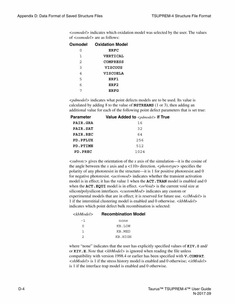
Appendix D: Data Format of Saved Structure Files TSUPREM-4 Structure File Format

<oxmodel> indicates which oxidation model was selected by the user. The values of <oxmodel> are as follows:

<pdmodel> indicates what point defects models are to be used. Its value is calculated by adding 8 to the value of NSTREAMS (1 or 3), then adding an additional value for each of the following point defect parameters that is set true:

<subrotc> gives the orientation of the x axis of the simulation—it is the cosine of the angle between the x axis and a <110> direction. <phototype> specifies the polarity of any photoresist in the structure—it is 1 for positive photoresist and 0 for negative photoresist. <activmod> indicates whether the transient activation model is in effect; it has the value 1 when the ACT.TRAN model is enabled and 0 when the ACT.EQUI model is in effect. <orVoid> is the current void size at silicon/polysilicon interfaces. <customMod> indicates any custom or experimental models that are in effect; it is reserved for future use. <clModel> is 1 if the interstitial clustering model is enabled and 0 otherwise. <kbModel> indicates which point defect bulk recombination is selected:

where “none” indicates that the user has explicitly specified values of KIV.0 and/or KIV.E. Note that <kbModel> is ignored when reading the file unless compatibility with version 1998.4 or earlier has been specified with V.COMPAT. <shModel> is 1 if the stress history model is enabled and 0 otherwise; <itModel> is 1 if the interface trap model is enabled and 0 otherwise.

Oxmodel Oxidation Model0 ERFC

1 VERTICAL

2 COMPRESS

3 VISCOUS

4 VISCOELA

5 ERF1

6 ERF2

7 ERFG

Parameter Value Added to <pdmodel> if TruePAIR.GRA 16

PAIR.SAT 32

PAIR.REC 64

PD.PFLUX 256

PD.PTIME 512

PD.PREC 1024

<kbModel> Recombination Model-1 none

0 KB.LOW

1 KB.MED

2 KB.HIGH

D-4 Taurus™ TSUPREM-4™ User GuideN-2017.09

TSUPREM-4 Structure File Format Appendix D: Data Format of Saved Structure Files

Solution Values

The “s” line specifies which solution values are associated with each node of the structure. The (integer) value <nsol> specifies how many solution values are given, while <sol1> through <soln> give the names of the solutions that are present. Valid names in version 6.4 are: the names of the impurities (including user-defined impurities); the names of the impurities preceded by “a_”, indicating the active portion of the impurity concentration; the names of the impurities preceded by “gb_”, indicating the concentration of the impurity associated with polycrystalline grain boundaries; the names vacancy, interstitial, x.vel, y.vel, o2, h2o, trap, sxx, syy, sxy, rloop, dloop, lgrain, gorient, and tpoly. Note that this list of solutions is subject to change in future revisions of the program.

Nodes

The “n” lines specify the solution values at each node. For each point in the mesh, there is an “n” line for each material at the point. The (integer) value <cindex-1> gives the index of the coordinate, minus one, and the (integer) <region> specifies the region. Points on exposed surfaces must also have an ambient node, denoted by a region index of zero. For each node, the solution values are given by <val1> through <valn> (floating-point).

Example The following input produces the structure file shown in Figure D-1.

line x loc=0line x loc=1line y loc=0line y loc=1init boron=1e13deposit oxide thick=.2savefile out.file=test.str stop

This structure contains 6 grid points, 2 regions (silicon and oxide), 4 triangles, and 10 nodes (4 in silicon, 4 in oxide, and 2 ambient nodes). Solution values for boron concentration are given at each node. No last processing temperature was specified, and the VERTICAL oxidation model and the PD.FERMI point defect model were used.

s <nsol> <sol1> <sol2> ... <soln>

n <cindex-1> <region> <val1> ... <valn>

Taurus™ TSUPREM-4™ User Guide D-5N-2017.09

Appendix D: Data Format of Saved Structure Files TSUPREM-4 Structure File Format

Older Versions of TSUPREM-4

This section describes differences between the current TSUPREM-4 structure file format and that used in older versions of the program.

Regions In versions 6.0 and earlier, regions were identified by a <material> code:

Figure D-1 TSUPREM-4 structure file

v TMA TSUPREM-4 (1999.2S)c 1 0 0 0c 2 0 0.99999997 0c 3 0.99999997 0 0c 4 0.99999997 0.99999997 0c 5 0 -0.19999999 0c 6 0.99999997 -0.19999999 0e 1 2 1 0e 2 4 2 0e 3 3 4 0e 4 5 6 2e 5 1 5 0e 6 6 3 0e 7 3 1 0r 1 siliconb 1b 7b 3b 2r 2 oxideb 4b 6b 7b 5t 1 1 1 3 2 2 -1024 4t 2 1 3 4 2 -1024 1 -1024t 3 2 1 5 6 -1022 4 -1024t 4 2 1 6 3 -1024 1 3M 0 12 1073.16 1 9 1.000000 0 0 0 0 1 0 0 1s 2 boron a_boronn 0 1 1.000000e+13 1.0000e+13n 0 2 1.000000e+05 1.0000e+05n 1 1 1.000000e+13 1.0000e+13n 2 1 1.000000e+13 1.0000e+13n 2 2 1.000000e+05 1.0000e+05n 3 1 1.000000e+13 1.0000e+13n 4 2 1.000000e+05 1.0000e+05n 4 0 1.000000e+05 1.0000e+05n 5 2 1.000000e+05 1.0000e+05n 5 0 1.000000e+05 1.0000e+05

<material> Material1 oxide

2 nitride

3 silicon

D-6 Taurus™ TSUPREM-4™ User GuideN-2017.09

TSUPREM-4 Structure File Format Appendix D: Data Format of Saved Structure Files

ModelParameters

In versions 8926 and before <nadd> and the parameters that follow are omitted. In versions 9035 and 5.0 <nadd> is 3, and the <temperature>, <oxmodel>, and <pdmodel> parameters are present. Starting with version 5.2, <nadd> is 5, and the “M” line includes the <subrotc> and <phototype> parameters. Starting with version 6.2, <nadd> is 6 and the “M” line includes the <activmod> parameter. Starting with version 6.3, <nadd> is 7 and the “M” line includes the <orVoid> parameter. Starting with version 6.4, <nadd> is 8 and the “M” line includes the <customMod> parameter. Starting with version 6.5, <nadd> is 10 and the “M” line includes the <clModel> and <kbModel> parameters. Starting with version 6.6, <nadd> is 12 and the “M” line includes the <shModel> and <itModel> parameters. Starting with version 1999.2, -1 is a valid value for <kbModel>.

In versions of TSUPREM-4 prior to version 6.0 the value of <pdmodel> is interpreted as follows:

Solution Values In versions 6.0 and earlier, <sol1> through <soln> are integer values indicating which solution values are present:

4 polysilicon

5 oxynitride

6 aluminum

7 photoresist

8 ambient (included void)

<material> Material

<pdmodel> Point Defect Model0 TWO.DIM (PD.TRANS)

2 FERMI (PD.FERMI)

4 STEADY (Obsolete;PD.TRANS used instead)

<solx> Solution0 vacancy concentration1 interstitial concentration2 arsenic concentration3 phosphorus concentration4 antimony concentration5 boron concentration6 steady-state vacancy concentration7 steady-state interstitial concentration8 x component of flow velocity9 y component of flow velocity10 oxidant concentration (dry O2)11 oxidant concentration (wet O2)12 concentration of filled interstitial traps15 Sxx component of stress

Taurus™ TSUPREM-4™ User Guide D-7N-2017.09

Appendix D: Data Format of Saved Structure Files Medici Structure File Format

Nodes In version 6.0 and earlier, <region> specifies a material index rather than a region index. The same values are used to identify materials as are used in the “r” lines.

Medici Structure File FormatThis section describes the output file format produced by the “SAVEFILE MEDICI” statement in TSUPREM-4. The TSUPREM-4 Medici file contains numerical values only. Floating point values use an exponent, denoted by “e”. Integer values do not have an exponent or a decimal point. Values are separated by spaces. The format of the file is as follows.

Line 1:

This line specifies the number of points in the grid <npt>, the number of triangular elements <ntri>, and the number of electrode points <nelpt>.

Line 2:

This line specifies the number of electrodes <nelec> and the number of materials in the structure <nmat>. Note that the number of materials is preceded by a minus sign. TSUPREM-4 converts all points on an interface with aluminum to electrodes.

Lines 3 through <npt>+2:

These lines specify the x and y coordinates <xcoord> and <ycoord> of each mesh point (in centimeters), the net n-type doping <cnet> (in atoms/cm3), and the total doping <ctotal> (in atoms/cm3). Note that a negative value of <cnet> indicates a p-type region. <xcoord>, <ycoord>, <cnet>, and <ctotal> are all floating-point values.

Lines <npt>+3 through <npt>+<ntri>+2:

16 Syy component of stress17 Sxy component of stress20 active component of arsenic concentration21 active component of phosphorus concentration22 active component of antimony concentration23 active component of boron concentration

<solx> Solution

<npt> <ntri> <nelpt>

<nelec> -<nmat>

<xcoord> <ycoord> <cnet> <ctotal>

<reg> <p1> <p2> <p3>

D-8 Taurus™ TSUPREM-4™ User GuideN-2017.09

Medici Structure File Format Appendix D: Data Format of Saved Structure Files

These lines specify the triangular elements that make up the mesh. <reg> is the region number for the element. (Regions are numbered consecutively, starting at one.) <p1>, <p2>, and <p3> are the indices of the points at the vertices of the triangular element. The points are specified in a clockwise order, when viewed in a left-handed coordinate system (that is, x increasing from left to right and y increasing from top to bottom).

Lines <npt>+<ntri>+3 through <npt>+<ntri>+<nelpt>+2:

These lines specify the electrode <elec> associated with each electrode point <ept>. <elec> is either a name (assigned with the ELECTRODE statement) or a number. (Electrode numbers start at one and increasing to <nelec>, as needed.)

Line <npt>+<ntri>+<nelpt>+3 (last line in file):

This line specifies the material associated with each region in the structure:

Example The following TSUPREM-4 input produces the structure file shown in Figure D-2:

line x loc=0line x loc=1line y loc=0line y loc=1init boron=1e13deposit oxide thick=.2deposit aluminum thick=.1select z=0 temp=800savefile medici out.file=testpi.strstop

<ept> <elec>

<mat1> <mat2> ... <matn>

<matx> Material-6 oxynitride-4 unspecified insulator (for example, photoresist)-2 nitride-1 oxide1 silicon3 polysilicon4 unspecified semiconductor

Taurus™ TSUPREM-4™ User Guide D-9N-2017.09

Appendix D: Data Format of Saved Structure Files Medici Structure File Format

Figure D-2 Medici structure file

6 4 2 1 -2 0.000000e+00 0.000000e+00 -1.000000e+13 1.000000e+13 0.000000e+00 1.000000e-04 -1.000000e+13 1.000000e+13 1.000000e-04 0.000000e+00 -1.000000e+13 1.000000e+13 1.000000e-04 1.000000e-04 -1.000000e+13 1.000000e+13 0.000000e+00 -2.000000e-05 0.000000e+00 0.000000e+00 1.000000e-04 -2.000000e-05 0.000000e+00 0.000000e+00 1 1 3 2 1 3 4 2 2 1 5 6 2 1 6 3 5 1 6 1 1 -1

D-10 Taurus™ TSUPREM-4™ User GuideN-2017.09

APPENDIX E

Using the MINIMOS 5 InterfaceE

This appendix explains how to send TSUPREM-4 results to the MINIMOS 5 device simulator. It should be used in conjunction with the SAVEFILE input statement described Chapter 4, SAVEFILE, p. 4-77.

Overview of the TSUPREM-4 Interface to MINIMOS 5The interface is file-oriented and unidirectional (from TSUPREM-4 to MINIMOS 5), and consists of three separate steps.

1. TSUPREM-4 writes a formatted file (that is, ASCII or EBCDIC). This file contains a 2-D doping profile of the source area (and optionally the drain area) of the device being simulated. (See Step 1: Directing TSUPREM-4 to Generate a Formatted File, p. E-2.)

2. Use a separate standalone FORTRAN program (named mmatob) to convert the formatted file to a FORTRAN binary file. (See Step 2: Converting the Formatted File to FORTRAN Binary, p. E-6.)

3. Execute MINIMOS 5, which reads in the binary doping file. (See Step 3: Running MINIMOS 5, p. E-6.)

Throughout this discussion, use the convention that the source is on the left of the channel and the drain is on the right of the channel. Also, remember that TSUPREM-4 expects user-specified values in microns, while MINIMOS 5 expects centimeters.

All references to MINIMOS 5 refer to the program supplied by the Technical University of Vienna, Austria, Institute for Microelectronics, and the accompanying MINIMOS 5 User’s Guide, dated March 2, 1990.

Taurus™ TSUPREM-4™ User Guide E-1N-2017.09

Appendix E: Using the MINIMOS 5 Interface Step 1: Directing TSUPREM-4 to Generate a Formatted File

Step 1: Directing TSUPREM-4 to Generate a Formatted FileCentral to the preparation of the MINIMOS 5 output file is the concept of the MINIMOS 5 simulation region. This region is a subset of a simulated TSUPREM-4 device. While a TSUPREM-4 MOS device simulation may encompass an entire device, including the gate oxide, field oxide, and metallization layers, MINIMOS 5 expects to read a 2-D doping file encompassing only a portion of the full device. The X.MIN, X.MAX, Y.MIN, and Y.MAX parameters on the SAVEFILE statement are used to define a rectangular subset of the complete device. This subset is referred to as the MINIMOS 5 simulation region.

Defining the MINIMOS 5 Simulation Region

The MINIMOS 5 simulation region must be defined to include the source, drain, and channel of the MOS transistor; gate and field oxide regions are normally excluded. The MINIMOS 5 simulation region must be deep enough to include the source and drain junction depths, because MINIMOS 5 expects to see a change in the sign of the net doping concentration along both the left and right edges of its simulation space (except when simulating SOI devices).

The following TSUPREM-4 statement defines the MINIMOS 5 simulation region, and generates a formatted MINIMOS 5 file for the device shown in Figure E-1 (from Chapter 6, NMOS LDD Process, p. 6-2):

SAVEFILE MINIMOS5 OUT.FILE=MMDOPF FULL.DEV+X.MIN=-2 X.MAX=2 Y.MIN=0.0174 Y.MAX=1.5+X.MASK.S=-0.57 X.MASK.D=0.57

The parameter MINIMOS5 specifies that the file to be produced is a formatted 2-D doping file, to be read by MINIMOS 5. OUT.FILE=MMDOPF specifies that the formatted doping file is named MMDOPF. Because this is the filename expected by the file conversion program mmatob (discussed later in this section), it is the recommended name to use when directing TSUPREM-4 to prepare a MINIMOS 5 doping file.

In Figure E-1, you see a complete device with source, channel, and drain regions, so the FULL.DEV parameter should be specified. If the TSUPREM-4 simulation encompasses only the source half of a device, use HALF.DEV. If the TSUPREM-4 simulation is for the drain half of a device, reflect the TSUPREM-4 structure to create a complete device and specify FULL.DEV. Because the drain region is assumed to be to the right of the channel, use the statement:

STRUCTURE REFLECT LEFT

(preceding the STRUCTURE MINIMOS5 statement) to reflect the device at its left edge (the center of the channel), thus creating a complete device.

E-2 Taurus™ TSUPREM-4™ User GuideN-2017.09

Step 1: Directing TSUPREM-4 to Generate a Formatted File Appendix E: Using the MINIMOS 5 Interface

The X.MIN, X.MAX, Y.MIN, and Y.MAX parameters define the left, right, top, and bottom edges of the MINIMOS 5 simulation region, respectively. The assigned values for X.MIN and X.MAX are chosen by visual inspection of Figure E-1 and need not be exact. X.MIN is roughly centered between the left-most field oxide and the gate, in an area where the impurity contours are essentially flat. If X.MIN is too far to the left, the field oxide region is included. X.MAX is assigned the corresponding value on the right side of the structure.

Similar to X.MIN and X.MAX, Y.MAX is determined based on visual inspection of Figure E-1 and need not be exact. However, Y.MAX must be deep enough in the structure to include the source and drain junction depths, or MINIMOS 5 issues the error message:

DOPING PROFILE INCONSISTENT

Y.MAX should also be deep enough in the structure to include the depletion region for the maximum bias to be applied, particularly if the dopant profile is still changing at that depth.

The values used for X.MIN, X.MAX, and Y.MAX are not critical, because if MINIMOS 5 needs a simulation region that is larger than the one defined by the doping file, MINIMOS 5 extends the profiles in the required direction. However, the value assigned to Y.MIN is critical, because MINIMOS 5 interprets Y.MIN as the gate oxide/silicon interface. Thus, Y.MIN has a physical significance and should be carefully determined. For TSUPREM-4 MOSFET simulations, the gate oxide/silicon interface is typically found just below y=0.0. Therefore, as a first approximation, the default value (Y.MIN=0.0) could be used. Another approximation could be obtained from visual inspection of a 2-D plot.

Figure E-1 NMOS structure to be transferred to MINIMOS 5

-4.00 -2.00 2.00Distance (µm)

Dis

tanc

e (µ

m)

2.00

-2.0

0

0.00 4.00

Silicon Polysilicon Oxide Aluminum

Taurus™ TSUPREM-4™ User Guide E-3N-2017.09

Appendix E: Using the MINIMOS 5 Interface Step 1: Directing TSUPREM-4 to Generate a Formatted File

However, the most accurate value is obtained by using the following pair of TSUPREM-4 statements:

SELECT Z=1PRINT.1D LAYERS X.VALUE=<xchan>

where <xchan> is the x-coordinate of the vertical slice along which values are to be printed. In a typical TSUPREM-4 MOSFET simulation (such as Figure E-1), the gate oxide/silicon interface is bowed slightly upwards and is closest to y=0.0 in the middle of the channel. For such cases, <xchan> in the preceding code fragment should be the x coordinate of the middle of the channel. The center of the channel for the device shown in Figure E-1 is at x=0.0. Thus, the TSUPREM-4 statements:

SELECT Z=1PRINT.1D LAYERS X.VALUE=0.0

are used to generate the following TSUPREM-4 output (results may vary slightly on your system):

From this output, note that the bottom of the oxide layer occurs at y=0.0174 microns, so Y.MIN=0.0174 is used. Also, note that the thickness of the insulating oxide is 0.0419 microns (419 Å). This value is used on the MINIMOS 5 DEVICE directive when specifying a value for the TINS parameter.

There is no need to specify X.CHANNE in this example, because the default value (midway between X.MIN and X.MAX) is appropriate. X.CHANNE is only needed if an asymmetric device is simulated, and serves to divide the MINIMOS 5 simulation region into a source half and a drain half.

The two remaining parameters, X.MASK.S and X.MASK.D, are similar to Y.MIN in that they have a physical significance. X.MASK.S is the x coordinate of the mask edge in the source area of the MINIMOS 5 simulation region. MINIMOS 5 interprets this coordinate as the left edge of the gate electrode and treats X.MASK.D as the right edge of the gate electrode. Values for these parameters can be obtained by visual inspection of Figure E-1. For more accuracy, use the following pair of TSUPREM-4 statements:

SELECT Z=YPRINT.1D POLY /OXIDE

to print the x and y coordinates of the interface between the polysilicon gate contact and the gate oxide. From this output (not shown), you will find that X.MASK.S=-0.57 and X.MASK.D=0.57.

The SGAP and DGAP parameters on the MINIMOS 5 DEVICE directive are used to specify the gap between the gate and source contact and the gap between the gate and drain contacts, respectively.

Num Material Top Bottom Thickness Integral 1 oxide -1.1111 -0.4107 0.7004 7.0040e-05 2 polysilicon -0.4107 -0.0245 0.3862 3.8615e-05 3 oxide -0.0245 0.0174 0.0419 4.1938e-06 4 silicon 0.0174 200.0000 199.9826 1.9998e-02

E-4 Taurus™ TSUPREM-4™ User GuideN-2017.09

Step 1: Directing TSUPREM-4 to Generate a Formatted File Appendix E: Using the MINIMOS 5 Interface

The TSUPREM-4 statements:

SELECT Z=YPRINT.1D SILICON /OXIDE

can be used to print the x and y coordinates of the silicon/oxide interface, as an aid to determining SGAP and DGAP for the subsequent MINIMOS 5 run. Alternatively, the values could be approximated by visual inspection of Figure E-1.

Notes on the Size of the MINIMOS 5 Simulation Region

The X.MIN, X.MAX, Y.MIN, and Y.MAX parameters determine the size of the MINIMOS 5 simulation region. If this region is large, containing many TSUPREM-4 grid points, the preparation of the MINIMOS 5 doping file could take several minutes. Additionally, the subsequent MINIMOS 5 run can take more execution time if the doping file defines a large simulation region. For these reasons, you should attempt to keep the MINIMOS 5 simulation region reasonably small when choosing X.MIN, X.MAX, Y.MIN, and Y.MAX. This also reduces the size of the doping file.

The standard version of MINIMOS 5 expects the doping file to contain from 10 to 80 horizontal grid lines and from 10 to 80 vertical grid lines. Normally, this requirement is satisfied automatically by TSUPREM-4 during the preparation of the doping file. However, certain choices for X.MIN, X.MAX, Y.MIN, and Y.MAX can result in a TSUPREM-4 warning message stating that there are too many (or too few) grid lines. Unless the version of MINIMOS 5 you run has been modified to accept expanded limits, you must modify the X.MIN, X.MAX, Y.MIN, or Y.MAX values as advised in the TSUPREM-4 warning message and regenerate the doping file. Otherwise, when MINIMOS 5 attempts to read the doping file, it issues the error message:

DOPING FILE FORMAT ERROR

and terminates execution. You can also modify the number of grid lines by specifying the DX.MIN and/or DY.MIN parameters. These change the minimum grid spacings in the x and y directions from their default values of min((X.MAX - X.MIN)/80,0.01) and min((Y.MAX - Y.MIN)/80,0.01), respectively.

Nonplanar Oxide Regions in MINIMOS 5

As stated in the MINIMOS 5 User’s Guide, MINIMOS 5 can model nonplanar oxide regions. This is accomplished by including the GEOMETRY directive (and associated parameters) in the MINIMOS 5 input command file. However, the doping file (as dictated by MINIMOS 5) makes no provision for the inclusion of geometry information. As discussed, the doping file uses a single coordinate (Y.MIN) to specify the gate oxide/silicon interface, implying a planar device. Therefore, TSUPREM-4 cannot automatically export nonplanar geometry information to MINIMOS 5 by including it in the doping file—the MINIMOS 5

Taurus™ TSUPREM-4™ User Guide E-5N-2017.09

Appendix E: Using the MINIMOS 5 Interface Step 2: Converting the Formatted File to FORTRAN Binary

user must approximate the nonplanarities of the device simulated in TSUPREM-4 by hand, attempting to duplicate the TSUPREM-4 geometry in MINIMOS 5 by using the GEOMETRY directive. Fortunately, many devices (such as the MOSFET in Figure E-1) are approximately planar, and the MINIMOS 5 GEOMETRY directive is not required to simulate the intrinsic device operation. In such cases, assign Y.MIN to the top-most point of the silicon, as discussed earlier. Because the gate oxide/silicon interface is not absolutely flat, the left and right portions of the top of the MINIMOS 5 simulation region contain very thin layers of oxide. To correct this, TSUPREM-4 automatically ignores the impurity concentration in the oxide and extends the doping profile of the underlying silicon upward (using the concentration at the oxide/silicon interface). In general, TSUPREM-4 ignores the dopants in any nonsilicon material within the MINIMOS 5 simulation region, using instead the doping of the underlying silicon.

Step 2: Converting the Formatted File to FORTRAN BinaryTSUPREM-4 writes a formatted (that is, ASCII or EBCDIC) file for MINIMOS 5. However, MINIMOS 5 requires a FORTRAN binary doping file. The formatted file written by TSUPREM-4 is converted to FORTRAN binary by executing the standalone FORTRAN program named mmatob. This step is needed because of incompatibilities between binary files written by C programs (such as TSUPREM-4) and FORTRAN programs (such as MINIMOS 5) on some computer systems.

The current version of mmatob is executed by simply typing:

mmatob

followed by a carriage return. Note that mmatob expects to read a formatted file named MMDOPF and write a binary file named MMDOPB. The easiest way to assure that the formatted file is named MMDOPF is to specify OUT.FILE=MMDOPF on the TSUPREM-4 SAVEFILE statement used to generate the MINIMOS 5 file. Alternatively, rename or copy the formatted file to MMDOPF before executing mmatob. Any existing file named MMDOPB is overwritten when mmatob is executed.

Step 3: Running MINIMOS 5MINIMOS 5 reads the binary doping file from FORTRAN logical unit 20. Similarly, the input command file must be available on FORTRAN unit 15. Refer to your MINIMOS 5 documentation for instructions on how to associate these input files with the correct FORTRAN logical unit numbers.

E-6 Taurus™ TSUPREM-4™ User GuideN-2017.09

Step 3: Running MINIMOS 5 Appendix E: Using the MINIMOS 5 Interface

Figure E-2 shows a listing of a sample MINIMOS 5 input command file (EX2D.INP, included with standard versions of MINIMOS 5).

This file uses the PROFILE and IMPLANT directives to generate a doping profile. To convert EX2D.INP so that it reads an external 2-D doping file, the PROFILE statement is changed to:

PROFILE FILE=2-D

The IMPLANT directive, used in EX2D.INP to specify a channel implantation, is removed. In addition, the parameters and values specified on the DEVICE statement are modified as needed to match the geometry of the device simulated in TSUPREM-4. The resulting modified MINIMOS 5 input command file is shown in Figure E-3.

Recall that MINIMOS 5 expects dimensions in centimeters, not microns. To use MINIMOS 5 to simulate a nonplanar device, specify the GEOMETRY directive, as discussed earlier, in Nonplanar Oxide Regions in MINIMOS 5, p. E-5.

Notes on Using MINIMOS 5

Particular care must be taken when specifying the L parameter (gate electrode length) on the MINIMOS 5 DEVICE directive. The value assigned to L should correspond to the distance between the values assigned to TSUPREM-4 parameters X.MASK.S and X.MASK.D. For example, if X.MASK.S=-0.57 (microns) and X.MASK.D=0.57 (microns), the distance between them is 1.14 microns, so L=1.14e-4 (centimeters). In this case, specifying a value of L greater than 1.14e-4 centimeters has the effect of stretching the channel, and should not

Figure E-2 Listing of MINIMOS 5 command file EX2D.INP

EXAMPLE FOR CLASSICAL 2-D MODEL (EX2D.INP)DEVICE CHANNEL=N GATE=NPOLY TINS=150.E-8 W=1.E-4 L=0.85E-4BIAS UD=4. UG=1.5PROFILE NB=5.2E16 ELEM=AS DOSE=2.E15 TOX=500.E-8 AKEV=160.+ TEMP=1050. TIME=2700IMPLANT ELEM=B DOSE=1.E12 AKEV=12 TEMP=940 TIME=1000OPTION MODEL=2-DOUTPUT ALL=YESEND

Figure E-3 Listing of MINIMOS 5 command file EX2D.INP, modified to read doping profiles produced by TSUPREM-4

EXAMPLE FOR CLASSICAL 2-D MODEL (READS 2-D DOPING FILE)DEVICE CHANNEL=N GATE=NPOLY TINS=419E-8 W=1.E-4 L=1.14E-4+ DGAP=1.87E-4 SGAP=1.87E-4BIAS UD=4. UG=1.5PROFILE FILE=2-DOPTION MODEL=2-DOUTPUT ALL=YESEND

Taurus™ TSUPREM-4™ User Guide E-7N-2017.09

Appendix E: Using the MINIMOS 5 Interface Interpreting Error Messages

cause problems in MINIMOS 5. However, a value of L substantially smaller than 1.14e-4 centimeters could cause the source and drain profiles to overlap, effectively eliminating the channel. MINIMOS 5 responds with the error message:

DOPING PROFILE INCONSISTENT

and terminates execution.

Interpreting Error MessagesThe warning and error messages issued by TSUPREM-4 during the preparation of the doping file are clear and fairly detailed, recommending corrective action when necessary.

The following error messages from MINIMOS 5 may be encountered:

DOPING PROFILE INCONSISTENT

MINIMOS 5 issues this message for a variety of error conditions. This can occur when the L parameter on the MINIMOS 5 DEVICE directive is too small, causing the source and drain profiles to overlap, effectively eliminating the channel. Correct the error by using a value of L that is at least as large as the difference between the X.MASK.S and X.MASK.D parameters, as described above. The doping file does not need to be regenerated.

The above message can also occur when the MINIMOS 5 simulation region, as defined in TSUPREM-4, is not deep enough to include the junction depths in both the source and drain regions. Correct the error by using a larger value for Y.MAX on the TSUPREM-4 SAVEFILE statement. In this case, the doping file must be regenerated.

To avoid the above message when using TSUPREM-4 and MINIMOS 5 to simulate SOI devices, the MINIMOS 5 DEVICE directive must include the BULK, FILM, and KBULK parameters.

When too many (or too few) horizontal or vertical grid lines are present in the doping file, the following message can appear:

DOPING FILE FORMAT ERROR

TSUPREM-4 in this case should have issued a warning message, describing the problem and recommending corrective action. However, TSUPREM-4 went ahead and prepared a doping file after issuing the warning, in the event that your version of MINIMOS 5 has been modified to accept expanded limits. Correct the error by using different values for X.MIN, X.MAX, Y.MIN, or Y.MAX in TSUPREM-4, and regenerate the doping file.

E-8 Taurus™ TSUPREM-4™ User GuideN-2017.09

GLOSSARY

Glossary

This glossary contains terms frequently used in the Taurus™ TSUPREM-4™ User Guide. A list of acronyms is included as the last section in the Glossary. For references to more information about a term, see the Index.

A

activation of dopants Movement of dopant atoms onto substitutional sites on the silicon lattice where they are electrically active.

adaptive gridding Automatic adaptation of the simulation mesh by the program to improve solution accuracy.

amorphization The complete disruption of the silicon lattice structure caused by ion implantation. The amorphized region will recrystallize (through epitaxial regrowth) during the next high-temperature step, but residual damage may remain, especially at the edges of the amorphized layer.

analytical oxidationmodel

A model that uses empirical descriptions of the 2-D oxide shape to predict the results of local oxidation steps.

automatic meshgeneration

Generation of the simulation mesh automatically by the program based on general guidelines supplied by the user.

C

channeling Tendency of ions to travel along open directions in the silicon lattice during implantation. Channeling may cause implanted profiles to be deeper than expected, depending on the tilt and rotation of the wafer related to the ion beam. The effect is included in the dual Pearson implant tables and in the Monte Carlo implant model.

clustering The formation of groups of atoms whose properties are different from the properties of the individual atoms within the group. Clustering usually refers to the clustering of dopant atoms to form immobile and electrically inactive complexes. (See interstitial clustering.)

Taurus™ TSUPREM-4™ User Guide Glossary-1N-2017.09

Glossary

D

deposition One of the basic fabrication steps used for IC processing. TSUPREM-4 contains a simple model for deposition of conformal layers. If more advanced models are needed, TSUPREM-4 can be used with Taurus Topography.

diffusion Spreading of impurities due to random motion at high temperatures. The term also refers to any process step in which diffusion occurs. TSUPREM-4 includes detailed physical models for diffusion and other processes, such as oxidation and silicidation, that occur during high temperature fabrication steps.

damage annealing Removal of implantation damage with high temperatures.

dislocation loops A class of extended defect in the silicon lattice structure. The ED-AAM models end-of-range dislocation loops produced by amorphizing ion implants.

dopant An impurity added to a structure to control its electrical properties.

E

epitaxial growth Growth of single crystal silicon on top of an existing silicon structure. TSUPREM-4 includes a model for epitaxial growth on planar substrates.

epitaxial regrowth Recrystallization of a silicon region amorphized during ion implantation.

G

grid (See mesh.)

I

implant damage Damage to the silicon lattice structure caused by ion implantation.

impurity Any atom other than silicon in a silicon structure. Often used to refer to a dopant.

interstitial A type of point defect consisting of an extra silicon atom not on the lattice site. Interstitials promote diffusion by pairing with dopants.

interstitial clustering Clustering of interstitials. Clustered interstitials are assumed to be immobile and do not promote the diffusion of impurities. In TSUPREM-4, the clustering model is used to simulate the effects of {311} defects.

interstitial trapmodel

A model describing the absorption and release of interstitials at a trapping site.

ion implantation Introduction of dopants into a wafer by a beam of accelerated ions.

ion pairing Coupling of dopant atoms of opposite charge to form an immobile pair.

Glossary-2 Taurus™ TSUPREM-4™ User GuideN-2017.09

Glossary

TN

L

local oxidation Oxidation of a portion of the silicon surface, achieved by masking the portion that is not oxidized with a material such as silicon nitride.

M

mesh The array of points within the structure at which solution values are numerically calculated. (The term is used interchangeably with grid.)

Monte Carlo implantmodel

A physics-based model that uses statistical techniques to calculate impurity and damage profiles produced by ion implantation.

N

numerical oxidationmodel

A model that uses the numerical solution of the physical equations for oxide growth and flow to predict the results of arbitrary oxidation steps.

O

oxidation Creation of silicon dioxide by reaction of silicon or polysilicon with oxygen. Oxidation is modeled in TSUPREM-4 whenever diffusion occurs in an oxidizing ambient.

point defects A localized defect (as opposed to an extended defect) in a silicon lattice structure. In TSUPREM-4, the term point defects refers to interstitials (that is silicon self-interstitials) and vacancies.

polycrystallinemodel

A model for polycrystalline materials used primarily for modeling polycrystalline silicon. It includes models for grain growth and the effect of grain boundaries on dopant diffusion.

P

PMEI Physical model and equation interface. PMEI is intended to be an universal language for scripting models and equations for semiconductor process and device simulation.

S

segregation Transport of an impurity across an interface between two materials due to a difference in chemical potential. This transport results in an equilibrium ratio of impurity concentration across a material boundary.

aurus™ TSUPREM-4™ User Guide Glossary-3-2017.09

Draft 8/9/17

Glossary

silicidation Interaction of silicon to form a metal silicide. Modeled in TSUPREM-4 by the DIFFUSION statement whenever necessary materials are present in the structure.

solid solubility The concentration at which dopant atoms precipitate, becoming immobile and electrically active.

stress TSUPREM-4 includes models for calculating the physical stresses produced during fabrication. The stress history model simulates the stresses produced by oxidation, thermal mismatch between materials, intrinsic strain in deposited layers, and surface tension.

T

TED Transient-enhanced diffusion. Enhanced diffusion caused by implant damage.

TSUPREM-4 The name originated from a combination of TMA (now the TCAD Business Unit of Synopsys) and SUPREM-IV, the Stanford University Process Engineering Models.

U

USEIT User-specified equation interface is an optionally available capability for TSUPREM-4 that helps to quickly develop and evaluate process models.

Acronyms

LDD Lightly doped drain

MOS Metal-oxide semiconductor

NMOS N-channel metal-oxide semiconductor

OED Oxidation-enhanced diffusion

PMEI Physical Model and Equation Interface

TED Transient-enhanced diffusion

USEIT User-Specified Equation Interface

Glossary-4 Taurus™ TSUPREM-4™ User GuideN-2017.09

INDEX

TN

IndexNumerics1D bipolar example

completing the active region simulation ......... 5-9DEPOSITION statement ................................. 5-6EPITAXY statement ........................................ 5-6ERFC oxidation model .................................... 5-4ETCH statement ............................................... 5-5final structure ................................................ 5-11IMPLANT statement ........................................ 5-5initial active region ......................................... 5-3INITIALIZE statement ................................. 5-4input file sequence .......................................... 5-2LABEL statement ............................................ 5-6mesh generation .............................................. 5-4model selection ............................................... 5-4overview ......................................................... 5-2PD.FERMI point defect model ....................... 5-4PD.TRANS point defect model ....................... 5-5PLOT.1D statement .................................5-6, 5-8plotting the results .......................................... 5-6point defect model .......................................... 5-5printing layer information ............................... 5-8processing steps .............................................. 5-5SAVEFILE statement ...................................... 5-6saving the structure ......................................... 5-6SELECT statement ...................................5-6, 5-7VERTICAL oxidation model ........................... 5-4

1D simulation of simple structuresoverview ....................................................... 3-13tutorial example of .......................................... 5-2

2D diffusion with point defectsautomatic grid generation ............................. 5-20contour of boron concentration ..................... 5-21field implant .................................................. 5-20grid plot ......................................................... 5-21

lateral distribution of point defects ............... 5-25oxidation ....................................................... 5-20shaded contours of interstitial concentration 5-25using the FOREACH statement ....................... 5-23vertical distribution of point defects ............. 5-24

5-stream diffusion model .................................. 7-26

Aabsorption of interstitial traps ........................... 3-76activation of dopants ......................................... 3-38ACTIVE ............................................................... 7-8active region simulation

LDD implant ................................................... 6-8modeling polysilicon ....................................... 6-7oxide spacer and source/drain implant ............ 6-9plots ............................................................... 6-11source/drain contacts ....................................... 6-9

adaptive grid parameters, default coefficients . A-27adaptive gridding

advanced examples of ............................6-4, 6-28analytical implant models ........................... 4-228disable ......................................................... 4-228overview ........................................................ 3-10tutorial example of .......................................... 5-4

adding expressions to equations ......................... 7-5advanced examples

CMOS process .............................................. 6-31DMOS power transistor ................................ 6-40MOSFET with self-aligned silicides ............. 6-50NMOS LDD process ....................................... 6-2poly-buffered LOCOS .................................. 6-27polysilicon emitter study ............................... 6-54SOI MOSFET ............................................... 6-46trench implant simulation ............................. 6-18

advantages of intermediates ................................ 7-7AMBIENT ........................................................ 4-236

additional notes ........................................... 4-253chlorine ....................................................... 4-251coefficients .................................................. 4-251

aurus™ TSUPREM-4™ User Guide Index-1-2017.09

Index

coefficients chlorine examples ....................4-251COMPRESS model .....................................4-249description ...................................................4-248ERFC model ................................................4-248ERFG model ................................................4-248examples ......................................................4-252INITIAL parameter, 1D bipolar example .......5-5orientation ...................................................4-252oxidation models .........................................4-248oxidation models, polycrystalline silicon ....4-248oxidizing species .........................................4-252parameter dependencies ..............................4-252specified material ........................................4-252specified units ..............................................4-252stress dependence ........................................4-249VERTICAL model ......................................4-249VISCOELA model ......................................4-249VISCOUS model .........................................4-249

ambient gaschlorine example ...........................................3-17chlorine, coefficient tables ............................3-17defaults ..........................................................3-16oxidation of materials ....................................3-16pressure .........................................................3-15specifying characteristics ..............................3-15

amorphous implant calculation .......................3-154electronic stopping ......................................3-156ion beam width ............................................3-150nuclear stopping ..........................................3-155

analytic damage model ....................................3-144damage distribution calculations .................3-144recommended usage and limitations ...........3-145

analytic ion implant models ............................3-135analytic damage model ................................3-144depth-dependent lateral distribution ............3-143dose-dependent implant profiles .................3-140dual Pearson distribution .............................3-139Gaussian distribution ...................................3-138implant moment tables ................................3-136implanted impurity distributions .................3-135lateral distribution .......................................3-142multilayer implants ......................................3-142Pearson distribution .....................................3-138tilt and rotation tables ..................................3-141wafer tilt and rotation ..................................3-143

analytical oxidation models .............................3-101ERF1 model .................................................3-105ERF2 model .................................................3-106ERFC model .................................................3-104ERFG model .................................................3-107

linear rate .................................................... 3-102overview ..................................................... 3-101oxide growth rate ........................................ 3-102parabolic rate .............................................. 3-103thin regime .................................................. 3-102usage ........................................................... 3-104

annealingdamage ........................................................ 3-150in situ .......................................................... 3-150self-annealing ............................................. 3-150

ANTIMONY ...................................................... 4-350additional notes ........................................... 4-356description .................................................. 4-355examples ..................................................... 4-355

application of user-specified models .................. 7-7Arora mobility model ..................................... 3-192array values

effect due to redefinition .............................. 4-35getting array values ....................................... 4-35redefinition of array elements ....................... 4-35

ARSENIC ........................................................ 4-357additional notes ........................................... 4-363description .................................................. 4-362examples ..................................................... 4-363

ARSENIC parameter, EPITAXY statement1D bipolar example ........................................ 5-6

ASSIGN ............................................................ 4-23additional ASSIGN notes .............................. 4-28ASSIGN and optimization ............................ 4-28ASSIGN with mathematical expressions ..... 4-27assign with mathematical expressions, using

N.EXPRESS ........................................... 4-28description .................................................... 4-26expansion of ASSIGNed variable ................. 4-28overriding variables ...................................... 4-29reading the external data file ........................ 4-29varying during statement looping ................. 4-27

authorization file s4auth ................................... 2-10automatic grid generation

custom defaults ............................................... 3-7overview ......................................................... 3-5parameters, default coefficients ....................A-26tutorial examples of ...............................5-4, 5-20

AXES parameter, PLOT.1D statement1D bipolar example ........................................ 5-7

AXES parameter, PLOT.2D statementlocal oxidation example ................................ 5-19

Index-2 Taurus™ TSUPREM-4™ User GuideN-2017.09

Index

BBF2 implant .................................................... 3-144BF2 implant profile Fig. ................................. 3-141binary scattering theory .................................. 3-150

Coulomb potential ...................................... 3-153dimensionless form ..................................... 3-152energy loss .................................................. 3-151scattering angle ........................................... 3-152universal potential ....................................... 3-153

bipolar emitter structure and as-implanted arsenic profiles, as plotted using s4ex11c.inp Fig. .....6-57

Boltzmann statistics ........................................ 3-189BORON ............................................................. 4-364

additional notes ........................................... 4-370description .................................................. 4-369examples ..................................................... 4-369

boron diffusionenhancement due to fluorine ....................... 3-124enhancement in oxides ................................ 3-121enhancement in thin oxides ........................ 3-122

BORON parameter, INITIALIZE statement1D local oxidation example .......................... 5-20

boron-interstitial clustering model with small clusters ................................................................. 7-20

BOTTOM parameter, PLOT.1D statementlocal oxidation example ................................ 5-24

BOUNDARY ........................................................ 4-61description .................................................... 4-61example ......................................................... 4-62limitations ..................................................... 4-61

built-in keywords ................................................ 7-9

CC.COMPRE parameter, PLOT.2D statement

local oxidation example ................................ 5-17C.GRID parameter, PLOT.2D statement

local oxidation example ................................ 5-14C.TENSIO parameter, PLOT.1D statement

local oxidation example ................................ 5-17capacitance calculation ................................... 3-194

DC method .................................................. 3-194MOS capacitances ...................................... 3-195

Caughey mobility model ................................ 3-193CENTER parameter, LABEL statement

CMOS process example ............................... 6-38channel and source/drain doping profiles for SOI

MOSFET Fig. ........................................ 6-50

channel doping profile for NMOS transistor Fig. ....6-36

channeling ....................................................... 3-150channeling effects ........................................... 4-130charge state fractions ........................................ 3-69chemical predeposition ..................................... 3-17CLEAR parameter, PLOT.1D statement

1D bipolar example ......................................... 5-7CLEAR parameter, PLOT.2D statement

local oxidation example ................................ 5-25clustering and solid solubility, default coefficients .

A-7clustering model ................................................ 3-38CM parameter, LABEL statement

1D bipolar example ......................................... 5-8CMOS process example

0.8 micron device .......................................... 6-381.2 micron device .......................................... 6-39arsenic profiles in gate .................................. 6-38channel doping plot ....................................... 6-35COMPRESS model ......................................... 6-35contacts ......................................................... 6-35end of main loop ........................................... 6-36END statement ............................................... 6-36final mesh ...................................................... 6-38FOREACH loop .....................................6-31, 6-36FOREACH statement ...................................... 6-34INITIALIZE statement ............................... 6-36lightly doped drain structure ......................... 6-35main loop ...................................................... 6-33mesh generation ............................................ 6-33models ........................................................... 6-35overview ........................................................ 6-31PD.TRANS model ......................................... 6-35plotting results ............................................... 6-36processing ..................................................... 6-35SAVEFILE statement .................................... 6-36saving the structure ....................................... 6-36VERTICAL oxidation model ......................... 6-35

coefficient default values ................................... A-1COLOR ............................................................. 4-175

description ................................................... 4-176examples ..................................................... 4-176plot device selection .................................... 4-176

COLOR parameter, PLOT.1D statement1D bipolar example ......................................... 5-7

command input files ............................................ 2-4COMMENT ............................................................ 4-7

description ....................................................... 4-7examples ......................................................... 4-7

Taurus™ TSUPREM-4™ User Guide Index-3N-2017.09

Index

notes ................................................................4-7complete NMOS structure, plotted by input file

s4ex4c.inp Fig. ........................................6-13completing the active region simulation .............5-9

field oxidation ...............................................5-11reading a saved structure ...............................5-10

COMPRESS model ...........................................3-110boundary conditions ....................................3-111compressible viscous flow ..........................3-111material parameters .....................................3-111recommended usage ....................................3-111

compressible viscous flow ..............................3-111concentration dependence ...............................3-108concentration of point defects

versus depth, as plotted by input file s4ex2b.inp Fig. ..........................................................5-24

versus width, as plotted by input file s4ex2b.inp Fig. ..........................................................5-25

CONTOUR .........................................................4-173additional notes ...........................................4-174description ...................................................4-174example .......................................................4-174line type and color .......................................4-174

contours of boronafter analytic implant Fig. .............................6-21after Monte Carlo implant Fig. .....................6-25concentration produced by input file s4ex2b.inp

Fig. ..........................................................5-23contours of hydrostatic pressure

final poly-buffered LOCOS structure Fig. ....6-30plotted by statements in input file s4ex2a.inp Fig.

5-19contours of interstitial concentration, as plotted by

input file s4ex2b.inp Fig. ........................5-26contours of net doping for 1-micron and 2-micron

emitter stripes Fig. ..................................6-59contours of total arsenic concentration and poly grain

size after RTA Fig. .................................6-59CPULOG .............................................................4-49

description .....................................................4-49examples ........................................................4-49limitations ......................................................4-49

creating the initial structureadaptive gridding .............................................6-4masking information .......................................6-4setting the grid density ....................................6-3

creating the test structureautomatic grid generation ..............................5-29outline of example .........................................5-29

CRYSTAL parameter, IMPLANT statement

trench implant simulation example ..... 6-23, 6-25crystalline implant model

BF2 implantation ........................................ 3-160channeling ................................................... 3-150damage annealing ....................................... 3-150damage dechanneling ................................. 3-159lattice damage ............................................. 3-157lattice temperature ...................................... 3-156number of ions ............................................ 3-150

Ddamage annealing ........................................... 3-150DC method ..................................................... 3-194DEEP parameter, ELECTRICAL statement

NMOS LDD process example ...................... 6-15default coefficient notes ...................................A-32default coefficient tables

adaptive grid parameters ...............................A-27automatic grid generation parameters ..........A-26clustering and solid solubility .........................A-7electrical parameters .....................................A-20impurity parameters ........................................A-2material coefficients .....................................A-22Monte Carlo implant .....................................A-25notes ..............................................................A-32numerical methods ........................................A-25oxidation .......................................................A-12point defect parameters ...................................A-9polysilicon grain segregation ..........................A-7

default file names ............................................... 2-3DEFINE ............................................................ 4-45

description .................................................... 4-45examples ....................................................... 4-45format and syntax ......................................... 4-45usage notes .................................................... 4-46

DEPOSITION ................................................. 4-101additional notes ........................................... 4-107description .................................................. 4-104examples ..................................................... 4-106photoresist ................................................... 4-105polycrystalline materials ............................. 4-105structure bottom .......................................... 4-104

depositionincorporation of impurities .............. 3-173, 3-174layer thickness ............................................ 3-173overview ..................................................... 3-173photoresist type ........................................... 3-174

deposition parameters ..................................... 4-106DEVELOP ............................................. 4-110, 4-111

Index-4 Taurus™ TSUPREM-4™ User GuideN-2017.09

Index

description .................................................. 4-110example ....................................................... 4-110

DEVICE parameter, OPTION statement1D bipolar example ........................................ 5-7

device structure specification, input statementsBOUNDARY .................................................... 4-61ELECTRODE .................................................. 4-98ELIMINATE .................................................. 4-58INITIALIZE ............................................... 4-68LINE ............................................................. 4-56LOADFILE .................................................... 4-74MASK ............................................................. 4-87MESH ............................................................. 4-52PROFILE ...................................................... 4-89REGION ......................................................... 4-63SAVEFILE .................................................... 4-77STRUCTURE .................................................. 4-82

diagnostic output file s4dia ................................. 2-6DIFFUSION .................................................... 4-136

ambient gas ................................................. 4-139ambient gas parameters .............................. 4-140description .................................................. 4-139DRY02 parameter, 1D bipolar example ......... 5-6examples ..................................................... 4-141oxidation limitations ................................... 4-140reflow .......................................................... 4-140STEAM parameter, 1D bipolar example ........ 5-5THICKNES parameter, 1D bipolar example .. 5-6

diffusionactivation of impurities ................................. 3-35along grain boundaries ................................ 3-181anisotropic .................................................. 3-181clustering model ........................................... 3-38diffusion of impurities .................................. 3-18DIFFUSION statement ................................. 3-15grain boundary structure ............................. 3-180grain interiors .............................................. 3-180impurities .................................................... 3-172impurity fluxes .............................................. 3-18injection and recombination of point defects at

interfaces ................................................ 3-76interstitial traps ............................................. 3-80overview ....................................................... 3-14point defects .........................................3-67, 3-68segregation of impurities .............................. 3-63solution of equations ..................................... 3-17temperature ................................................... 3-15tutorial example of ........................................ 5-19

diffusion along boundaries ................................. 7-6diffusion enhancement in thinner oxides .......... 7-24

diffusion in PD.TRANS ..................................... 7-18diffusion of point defects

absorption of interstitial traps ....................... 3-76charge state fractions ..................................... 3-69equations ....................................................... 3-70equilibrium concentrations ............................ 3-68interstitial and vacancy diffusivities ............. 3-72net recombination rate of interstitials ........... 3-74reaction of pairs with point defects ............... 3-73

diffusivities ....................................................... 3-22dislocation loop model .............................3-97, 7-17

creation of ..................................................... 3-98effects of ........................................................ 3-99

DMOS power transistor exampleafter p-type body diffusion Fig. .................... 6-43COMPRESS oxidation model ......................... 6-41mesh generation ............................................ 6-41overview ........................................................ 6-40PD.TRANS point defect model ..................... 6-45processing DMOS structure .......................... 6-41summary ........................................................ 6-45

documentation and control, input statementsASSIGN ......................................................... 4-23COMMENT ........................................................ 4-7CPULOG ......................................................... 4-49DEFINE ......................................................... 4-45ECHO ............................................................. 4-39FOREACH/END ............................................. 4-14HELP ............................................................. 4-50IF/ELSEIF/ELSE/IF.END ...................... 4-21INTERACTIVE ............................................. 4-11INTERMEDIATE ........................................... 4-30L.MODIFY .................................................... 4-20LOOP/L.END ................................................ 4-16OPTION ......................................................... 4-40PAUSE ........................................................... 4-12RETURN ........................................................... 4-9SOURCE ........................................................... 4-8STOP ............................................................. 4-13UNDEFINE .................................................... 4-48

dopantsactivation of .................................................. 3-38advanced tutorial examples of .............6-21, 6-23diffusion of atoms equations ......................... 3-18dislocation loop model .................................. 3-97paired fractions .............................................. 3-26polycrystalline materials ............................. 3-179solid solubility ............................................... 3-35transient clustering model ............................. 3-38

DOSE parameter, IMPLANT statement

Taurus™ TSUPREM-4™ User Guide Index-5N-2017.09

Index

trench implant simulation example ...............6-23DRYO2 parameter, DIFFUSION statement

1D bipolar example .........................................5-6dual Pearson distribution .................................3-139DY parameter, DEPOSITION statement

SOI MOSFET example .................................6-47DY.OXIDE parameter, METHOD statement

local oxidation example ................................5-15DY.SURF parameter, MESH statement

CMOS process example ................................6-33

EE.RVCAP parameter, ELECTRICAL statement

NMOS LDD process example ......................6-16ECHO ..................................................................4-39

description .....................................................4-39examples ........................................................4-39

effective range model ......................................3-142electric field .......................................................3-20ELECTRICAL ..................................................4-198

additional notes ...........................................4-206description ...................................................4-203E.RVCAP parameter, NMOS LDD process

example ...................................................6-16examples ......................................................4-203files and plotting ..........................................4-203JUNCTION parameter, NMOS LDD process

example ...................................................6-16MOSCAP parameter, NMOS LDD process

example ......................................... 6-14, 6-15optimization examples ................................4-204quantum effect in CV plot ...........................4-205RESISTAN parameter, NMOS LDD process

example ...................................................6-14THRESHOLD parameter, NMOS LDD process

example ...................................................6-14electrical calculations

Arora mobility model ..................................3-192Boltzmann statistics ....................................3-189carrier mobility ............................................3-191Caughey mobility model .............................3-193Fermi-Dirac statistics ..................................3-189ionization of impurities ...............................3-190overview ......................................................3-188Poisson equation ..........................................3-189solution methods .........................................3-191tabular form .................................................3-192

electrical characteristics, plotted by input file s4ex4d.inp Fig. .......................................6-17

electrical data output files ................................... 2-8electrical extraction

MOS capacitance .......................................... 6-15plotting results of electrical extraction ......... 6-17source/drain junction capacitance ................. 6-16threshold voltage .......................................... 6-14

electrical parameters, default coefficients ........A-20ELECTRODE ..................................................... 4-98

additional notes ............................................. 4-99description .................................................... 4-98examples ....................................................... 4-99

ELIMINATE ..................................................... 4-58description .................................................... 4-58examples ....................................................... 4-59initial structure generation ............................ 4-59overlapping regions ...................................... 4-59reducing grid nodes ...................................... 4-59

enable/disable user-specified models ............. 4-227ENERGY parameter, IMPLANT statement

trench implant simulation example .............. 6-23environment variables ........................................ 2-4epitaxial growth

layer thickness ............................................ 3-171modeling ..................................................... 3-171overview ..................................................... 3-171

epitaxial regrowth ........................................... 3-185EPITAXY ........................................................ 4-142

ARSENIC parameter, 1D bipolar example .... 5-6description .................................................. 4-145example ....................................................... 4-146mobility tables ............................................ 4-146SPACES parameter, 1D bipolar example ....... 5-6TEMPERAT parameter, 1D bipolar example 5-6TIME parameter, 1D bipolar example ............ 5-6

epitaxyselective ...................................................... 3-172

EPITAXY parameter, TEMPERAT statement1D bipolar example ........................................ 5-6

EQUATION ...................................................... 4-233adding expressions to equations ..................... 7-5diffusion along boundaries ............................. 7-6flux at interfaces ............................................. 7-6initialization .................................................... 7-3new solution variable ...................................... 7-3solving method ............................................... 7-3update solution ................................................ 7-7

equilibrium concentrations ............................... 3-68ERF1 model .................................................... 3-105

initial structure ............................................ 3-105parameters ................................................... 3-105

Index-6 Taurus™ TSUPREM-4™ User GuideN-2017.09

Index

ERF2 model .................................................... 3-106initial structure ............................................ 3-105parameters ................................................... 3-105

ERFC model .................................................... 3-104ERFG model .................................................... 3-107

initial structure ............................................ 3-105parameters ................................................... 3-105recommended usage ................................... 3-107

ERR.FAC parameter, MESH statementNMOS LDD process example ........................ 6-4

ERR.FAC parameter, METHOD statement1D bipolar example ........................................ 5-4

error messages .................................................... 2-3ETCH

description .................................................. 4-113examples ..................................................... 4-116generate simulation structure ...................... 4-115removing regions ........................................ 4-113

etchingcomplex structures ...................................... 3-178defining the region ...................................... 3-175examples ..................................................... 3-177material removal ......................................... 3-176overview ..................................................... 3-175simple structure ........................................... 3-177structure with overhangs ............................. 3-178trapezoidal model ....................................... 3-176tutorial example .............................................. 5-5

examplesmask data file Fig. ..........................................C-2sensitivity plot for target with multiple data Fig. .

4-19trapezoidal etch model Fig. ........................ 3-178

EXPOSE .......................................................... 4-108description .................................................. 4-108OFFSET parameter ...................................... 4-108

extended defects AAMdislocation loop model .................................. 3-97transient clustering model ............................. 3-38

EXTRACT ........................................................ 4-185description .................................................. 4-190error calculation .......................................... 4-193examples ..................................................... 4-194extraction procedure ................................... 4-191file formats .................................................. 4-193optimization examples ................................ 4-196solution variables ........................................ 4-191targets for optimization ............................... 4-193

extract output files .............................................. 2-8

FFermi-Dirac statistics ...................................... 3-189field isolation simulation

displaying the plot ........................................... 6-5file specification .................................................. 2-3files

command input ................................................ 2-4default names .................................................. 2-3environment variables ..................................... 2-4input ................................................................ 2-4library .............................................................. 2-8mask data ........................................................ 2-5profile .............................................................. 2-5terminal output ................................................ 2-6types ................................................................ 2-3

final gridLDD NMOS example, produced by input files

s4ex4a.inp and s4ex4b.inp Fig. .............. 6-11SOI MOSFET Fig. ........................................ 6-49

final mesh0.8 micron NMOS structure Fig. .................. 6-38DMOS simulation, showing the result of adaptive

gridding Fig. ........................................... 6-45final profiles produced by input file s4ex1b.inp Fig.

5-11final structure

0.8 micron, NMOS structure, plotted by s4ex7b.inp Fig. ......................................................... 6-38

1.2 micron, NMOS, plotted by input file s4ex7c.inp Fig. ......................................................... 6-39

after removal of remaining titanium Fig. ...... 6-54DMOS power transistor, produced by input file

s4ex8.inp Fig. ......................................... 6-45NMOS plotted by file s4ex4b.inp Fig. .......... 6-12showing contours of net doping for SOI MOSFET

Fig. ......................................................... 6-49fine grids, final check .......................................... 6-1first part of input file

s4ex10.inp, NMOS transistor processing Fig. 6-51s4ex11c.inp, for plotting structure and contours of

as-implanted arsenic concentration Fig. 6-58, 6-61, ........................... 6-63, 6-64, 6-68, 6-70

s4ex2a.inp, for determining LOCOS shape Fig. ..5-13

s4ex2b.inp, showing processing steps Fig. ... 5-20s4ex3.inp, showing processing and plotting using

PD.FERMI point defect model Fig. ....... 5-27s4ex4a.inp, setting up grid for simulating NMOS

process Fig. .............................................. 6-3

Taurus™ TSUPREM-4™ User Guide Index-7N-2017.09

Index

s4ex4b.inp, showing polysilicon gate formation Fig. ............................................................6-8

s4ex4d.inp, showing threshold voltage extraction Fig. ..........................................................6-15

s4ex5.inp, showing grid setup Fig. ................6-18s4ex6.inp, Poly-buffered LOCOS process Fig. ....

6-28s4ex7a.inp, to set up grid for simulating CMOS

process Fig. .............................................6-31FLOW parameter, PLOT.2D statement

local oxidation example ................................5-16flux at interfaces ..................................................7-6flux at interfaces Fig. ..........................................7-6FOREACH/END ..................................................4-14

description .....................................................4-14examples ........................................................4-14notes ..............................................................4-15

formatinput statements ...............................................4-2mask data files ........................................C-1, D-1statement description .......................................4-4

Ggas

see DIFFUSION statement, ambient gasGaussian distribution .......................................3-138grain size model ..............................................3-182

concentration dependence ...........................3-184grain growth ................................................3-183grain surface energy ....................................3-184segregation drag ..........................................3-185

graphical output files ...........................................2-7graphics devices

default device ................................................. B-7determining which to use ............................... B-1modifying s4pcap ........................................... B-7output .............................................................. B-2supported devices ........................................... B-2

gridafter formation of isolation region, plotted by

s4ex4a.inp Fig. .........................................6-6plot produced by first PLOT.2D statement input

file s4ex2b.inp Fig. .................................5-21poly-buffered LOCOS application Fig. ........6-29trench implant example Fig. .........................6-19

grid generation parameters, automatic, default coefficients .............................................A-26

grid linesautomatic generation .......................................3-5

eliminating ...................................................... 3-5generated ......................................................... 3-4specifying ....................................................... 3-4

GRID parameter, PLOT.2D statementlocal oxidation example ....................... 5-14, 5-21

grid parameters, adaptive, default coefficients .A-27grid structure

1D simulation of simple structures ............... 3-13adaptive gridding .......................................... 3-10automatic generation ...................................... 3-5changes to mesh during processing ................ 3-7defining ........................................................... 3-3explicit specification ....................................... 3-3generated grid lines ......................................... 3-4initial impurity concentration ....................... 3-13initial impurity concentration, sheet resistance ....

3-14LINE statement ............................................... 3-4mesh ................................................................ 3-3nodes ............................................................... 3-3overview ......................................................... 3-3triangular elements ......................................... 3-3

GRID.FAC parameter, MESH statementCMOS process example ............................... 6-33DMOS power transistor example ................. 6-41local oxidation example ................................ 5-14NMOS DD process example .......................... 6-3

HH.RECTAN parameter, LABEL statement

local oxidation example ................................ 5-19HELP ................................................................. 4-50

description .................................................... 4-50example ......................................................... 4-50notes .............................................................. 4-50

HIGH parameter, ELECTRICAL statementNMOS LDD process example ...................... 6-15

IIF/ELSEIF/ELSE/IF.END .......................... 4-21

conditional operators .................................... 4-22description .................................................... 4-21expression for condition ............................... 4-22

IMPLANT ........................................................ 4-117boundary conditions ................................... 4-130channeling effects ....................................... 4-132CRYSTAL parameter, trench implant simulation

Index-8 Taurus™ TSUPREM-4™ User GuideN-2017.09

Index

example .................................................. 6-23description .................................................. 4-127DOSE parameter, trench implant simulation

example .................................................. 6-23ENERGY parameter, trench implant simulation

example .................................................. 6-23examples ..................................................... 4-132extended defects ......................................... 4-130Gaussian and Pearson distributions ............ 4-127Monte Carlo implant model ........................ 4-129MONTECAR parameter, trench implant

simulation example ................................ 6-19N.ION parameter, trench implant simulation

example .................................................. 6-23point defect generation ............................... 4-129table of range statistics ............................... 4-128TILT parameter, trench implant simulation

example .................................................. 6-19implant damage model .................................... 3-163

using ............................................................ 3-168implant, Monte Carlo, default coefficients ...... A-25impurities

activation of .................................................. 3-35clustering of .................................................. 3-35diffusion ...................................................... 3-172diffusion of ................................................... 3-18implantation .................................................. 3-66incorporation ............................................... 3-172interface trap model ...................................... 3-64ionization of ................................................ 3-190moving-boundary flux .................................. 3-64segregation coefficient .................................. 3-64segregation flux ............................................ 3-63segregation of ............................................... 3-63specifying ........................................................ 4-2transport coefficient ...................................... 3-64

IMPURITY ...................................................... 4-281description .................................................. 4-305examples ..................................................... 4-307impurity type ............................................... 4-305multiplication to diffusivity ........................ 4-306other parameters ......................................... 4-306solution options ........................................... 4-306

impurity distributions in bipolar structure at end input file s4ex1a.inp Fig. ................................... 5-8

impurity parameters, default coefficients .......... A-2IN.FILE parameter, INITIALIZE statement

1D bipolar example ...................................... 5-10incorporation of impurities ............................. 3-172informational output file s4inf ............................ 2-6

initial conditions ............................................. 3-131initial grid

accuracy .......................................................... 6-1for simulating DMOS power transistor Fig. . 6-41for simulating SOI MOSFET Fig. ................ 6-47for the 0.8 micron NMOS transistor, produced by

s4ex7a.inp Fig. ....................................... 6-34INITIAL parameter, AMBIENT statement

1D bipolar example ......................................... 5-5initialization ........................................................ 7-3initialization input file s4init ............................... 2-9INITIALIZE .................................................... 4-68

crystalline orientation .................................... 4-71description ..................................................... 4-70examples ....................................................... 4-72IN.FILE parameter, 1D bipolar example ...... 5-10Masetti’s mobility table ................................ 4-73mesh generation ............................................ 4-71previously saved structure files ..................... 4-71specifying initial doping .. 4-64, 4-71, 4-72, 4-75

injection rate ..................................................... 3-78input files ............................................................ 2-4

command ......................................................... 2-4mask data ........................................................ 2-5other ................................................................ 2-5profile .............................................................. 2-5s4ex1a.inp, simulating buried layer and epitaxial

deposition, bipolar transistor structure Fig. ...5-3

s4ex4c.inp, plotting final LDD NMOS structure Fig. ......................................................... 6-13

s4ex7b.inp, plotting results Fig. .................... 6-37s4init ................................................................ 2-9se4ex10p.inp, plotting results Fig. ................ 6-52

input statement descriptionsformat .............................................................. 4-2parameter types ............................................... 4-3specifying materials and impurities ................ 4-2statement description format ........................... 4-4syntax .............................................................. 4-2

INTERACTIVE ................................................. 4-11description ..................................................... 4-11example ......................................................... 4-11interactive input mode ................................... 4-11

interface functions ............................................. 7-13interface oxide breakup and epitaxial regrowth

oxide breakup .............................................. 3-185interface trap model .................................3-66, 7-19interface trap model, impurities ........................ 3-64INTERMEDIATE ............................................... 4-30

Taurus™ TSUPREM-4™ User Guide Index-9N-2017.09

Index

advantages of INTERMEDIATES ..................4-31advantages of intermediates ............................7-7array values ...................................................4-34comparison to ASSIGN .................................4-36value type ......................................................4-33

INTERSTITIAL .............................................4-319additional notes ...........................................4-335bulk and interface parameters .....................4-334description ...................................................4-334examples ......................................................4-334

interstitial and vacancy diffusivities ..................3-72interstitial clustering model ..................... 3-81, 7-15interstitial traps ..................................................3-80interstitial traps, enabling, disabling, and initialization

.................................................................3-80interstitials

absorption of traps .........................................3-76net recombination rate ...................................3-74

intrinsic stress in deposited layersstress history model .....................................3-131stress model .................................................3-131

ion implant data file s4imp0 ................................2-9ion implantation

advanced example of .....................................6-18analytic models ............................................3-135implant damage model ................................3-163Monte Carlo model .....................................3-147overview ......................................................3-134

ion pairing and mobile impurities .....................3-19ION parameter, IMPLANT statement

trench implant simulation example ...............6-23

JJCAP parameter, ELECTRICAL statement

NMOS LDD process example ......................6-14JUNCTION parameter, ELECTRICAL statement

NMOS LDD process example ......................6-16

Kkey files s4fky0 and s4uky0 ...............................2-10

LL.MODIFY ........................................................4-20

description .....................................................4-20LABEL .............................................................4-180

CM parameter, 1D bipolar example ................5-8

color ............................................................ 4-184description .................................................. 4-183examples ..................................................... 4-184label placement ........................................... 4-183line, symbol, and rectangle ......................... 4-183X parameter, 1D bipolar example .................. 5-8Y parameter, 1D bipolar example .................. 5-8

LAYERS parameter, PRINT.1D statementDMOS power transistor example ................. 6-43local oxidation example .................................. 5-9

library files ......................................................... 2-8authorization file s4auth ............................... 2-10initialization input file s4init .......................... 2-9ion implant data file, s4imp0 .......................... 2-9key files s4fky0 and s4uky0 .......................... 2-10plot device definition file s4pcap ................. 2-10

LINE ................................................................. 4-56additional notes ............................................. 4-57default regions and boundaries ..................... 4-57description .................................................... 4-56example ......................................................... 4-57maximum number of nodes and grid lines ... 4-57placing grid lines .......................................... 4-56structure depth and point defect models ....... 4-57

LINE.TYP parameter, CONTOUR statement1D local oxidation example .......................... 5-23

LINE.TYPE parameter, PLOT.1D statement1D bipolar example ........................................ 5-7

listingsinput file s4ex11a.inp for simulating bipolar

emitter structure Fig. .............................. 6-56input file s4ex1b.inp, showing statements

simulating the field oxide, base, and emitter region processing for bipolar transistor Fig. ..5-10

mask information read from file s4ex4m.tl1 Fig. .6-4

MINIMOS 5 command file EX2D.INP Fig. .. E-7MINIMOS 5 command file EX2D.INP, modified to

read doping profiles produced by TSUPREM-4 Fig. ........................................................... E-7

PRINT.1D command in file s4ex1a.inp Fig. . 5-9produced by PRINT.1D statement in input file

s4ex3.inp Fig. ......................................... 5-31LOADFILE ........................................................ 4-74

Taurus Lithography files ............................. 4-75description .................................................... 4-74examples ....................................................... 4-75user-defined materials and impurities .......... 4-75

local oxidation example

Index-10 Taurus™ TSUPREM-4™ User GuideN-2017.09

Index

COMPRESS oxidation model ......................... 5-20CONTOUR statement .............................5-18, 5-23DIFFUSION statement ........................5-15, 5-20diffusion with point defects .......................... 5-19END statement ......................................5-18, 5-23FOREACH statement .............................5-18, 5-23INITIALIZE statement ............................... 5-14LABEL statement .................................5-24, 5-25mesh generation ............................................ 5-14model selection ............................................. 5-15overview ....................................................... 5-12oxide shape ................................................... 5-12pad oxide and nitride layers .......................... 5-14PLOT.1D statement ...................................... 5-25plotting

mesh .......................................................... 5-14results ........................................................ 5-16stresses ...................................................... 5-17

PRINT.1D statement .................................... 5-19SAVEFILE statement .................................... 5-15SELECT statement ........................................ 5-18summary ....................................................... 5-26

LOOP/L.END ................................................... 4-16advantages .................................................... 4-19dependence and variability ........................... 4-17description .................................................... 4-17example ......................................................... 4-18parameter sensitivity ..................................... 4-17termination of optimization looping ............. 4-17

LOW parameter, ELECTRICAL statementNMOS LDD process example ...................... 6-15

LY.ACTIV parameter, MESH statementCMOS process example ............................... 6-33

LY.SURF parameter, MESH statementCMOS process example ............................... 6-33

MMASK ................................................................. 4-87

description .................................................... 4-87examples ....................................................... 4-88

mask data filesformat ..............................................................C-1overview ................................................. 2-5, C-1

MATERIAL ...................................................... 4-265description .................................................. 4-278examples ..................................................... 4-279POLYCRYS parameter, NMOS LDD process

example .................................................... 6-7viscosity and compressibility ...................... 4-279

material coefficients, default coefficients ........ A-22materials, specifying ........................................... 4-2mathematical functions ..................................... 7-11Medici

saved structure files overview ......................... 2-7Medici

MEDICI parameter ........................................ 4-81structure file format ........................................ D-8

Medici structure file Fig. ................................. D-10MESH ................................................................. 4-52

1D mode ........................................................ 4-55description ..................................................... 4-53examples ....................................................... 4-55grid creation methods .................................... 4-53GRID.FAC parameter, 1D bipolar example ... 5-4horizontal grid generation ............................. 4-54scaling the grid spacing ................................. 4-55scaling the grid spacing, GRID.FAC ............ 4-55vertical grid generation ................................. 4-54

meshchanges during processing .............................. 3-7DEPOSITION statement ................................. 3-7DEVELOP statement ........................................ 3-8EPITAXY statement ........................................ 3-7ETCH statement ............................................... 3-8overview .......................................................... 3-3oxidation and silicidation ................................ 3-9structure extension .......................................... 3-8

mesh generationdepositing a layer with nonuniform grid spacing

6-47DMOS power transistor, from input file s4ex8.inp

Fig. ......................................................... 6-40SOI MOSFET, from input file s4ex9.inp Fig. 6-46tutorial example .............................................. 5-4

mesh used for oxidation simulation Fig. .......... 5-13METHOD ........................................................... 4-210

adaptive gridding ........................................ 4-228analytical implant models ....................... 4-228disable ..................................................... 4-228

block solution .............................................. 4-230customizing the point defect models ........... 4-227description ................................................... 4-225enable/disable user-specified models .......... 4-227ERR.FAC parameter, 1D bipolar example ..... 5-4error tolerances ............................................ 4-231examples ..........................................4-232, 4-234fine control .................................................. 4-229grid spacing in oxide ................................... 4-225initial time step ............................................ 4-229

Taurus™ TSUPREM-4™ User Guide Index-11N-2017.09

Index

internal solution methods ............................4-229internal solution methods, changing ...........4-229matrix refactoring ........................................4-231matrix structure ...........................................4-231minimum-fill reordering ..............................4-230oxidation models .........................................4-225PD.FERMI model .......................................4-226PD.FULL model ..........................................4-226PD.TRANS model .......................................4-226point defect modeling ..................................4-226rigid versus viscous substrate ......................4-225solution method ...........................................4-231system solutions ..........................................4-230time integration ...........................................4-229

MINIMOS 5 interface ........................................ E-1miscellaneous functions ....................................7-14MOBILE ...............................................................7-9mobile impurities and ion pairing .....................3-19MOBILITY ......................................................4-313

analytic models ............................................4-317description ...................................................4-316example .......................................................4-317tables and analytic models ..........................4-317tables or model selection .............................4-317

models and coefficients, input statementsAMBIENT .....................................................4-236ANTIMONY ..................................................4-350ARSENIC .....................................................4-357BORON .........................................................4-364EQUATION ..................................................4-233IMPURITY ..................................................4-281INTERSTITIAL .........................................4-319MATERIAL ..................................................4-265METHOD .......................................................4-210MOBILITY ..................................................4-313MOMENT .......................................................4-254PHOSPHORUS ..............................................4-371REACTION ..................................................4-308VACANCY .....................................................4-336

modification of built-in functions .......................7-8ACTIVE ...........................................................7-8MOBILE ...........................................................7-9

MOMENT ...........................................................4-254additional notes ...........................................4-264description ...................................................4-260examples ......................................................4-264optional and required model parameters .....4-260using ............................................................4-261

Monte Carlo implantdefault coefficients .......................................A-25

model .......................................................... 3-147model, binary scattering theory .................. 3-150overview ....................................................... 6-23using ............................................................. 6-23

MONTECAR parameter, IMPLANT statementtrench implant simulation example ..... 6-19, 6-23

MOS capacitance ............................................ 3-195MOSCAP parameter, ELECTRICAL statement

NMOS LDD process example ...................... 6-14MOSFET with self-aligned silicides exampleCOMPRESS model ......................................... 6-51overview ....................................................... 6-50PD.FERMI model ......................................... 6-51preparation for silicidation ........................... 6-50silicidation .................................................... 6-51

MOSFET, quantum mechanical model .......... 3-193moving-boundary flux ............................. 3-64, 3-79multilayer implants ......................................... 3-142

dose matching ............................................. 3-142effective range model ................................. 3-142

NN20 oxidation

nitrogen trap and generation ....................... 3-120N2O oxidation ................................................ 3-120net recombination rate of interstitials ............... 3-74new solution variable .......................................... 7-3nitrogen trap and generation ........................... 3-120NMOS LDD process example

active region simulation ................................. 6-7COMPRESS oxidation model ........................... 6-5creating initial structure .................................. 6-2DEPOSITION statement ..........................6-7, 6-9DEVELOP statement .................................6-5, 6-7electrical extraction ...................................... 6-14ELIMINATE statement ................................... 6-2ETCH statement ............................................... 6-7formation of complete NMOS transistor ...... 6-12INITIALIZE statement ..........................6-2, 6-7LINE statement ............................................... 6-2MASK statement ........................................6-2, 6-7MESH statement ........................................6-2, 6-7METHOD statement .......................................... 6-7overview ......................................................... 6-2PD.FERMI model ........................................... 6-4PD.TRANS model ........................................... 6-5PLOT.2D statement ........................................ 6-5remove photoresist .......................................... 6-4SAVEFILE statement ................................... 6-11

Index-12 Taurus™ TSUPREM-4™ User GuideN-2017.09

Index

TRAP etch model ............................................ 6-5VERTICAL model ........................................... 6-4VISCOELA model ........................................... 6-5

NMOS parameter, ELECTRICAL statementNMOS LDD process example ...................... 6-14

NMOS structureafter LDD implant, as plotted by file s4ex4b.inp

Fig. ........................................................... 6-9to transfer to MINIMOS 5 Fig. ......................E-3

nodesaddition in growing oxide ............................... 3-9maximum number ........................................... 3-3overview ......................................................... 3-3regions where oxide is forming .................... 3-10removing in consumed silicon ........................ 3-9

numerical methods, default coefficients .......... A-25numerical oxidation models ............................ 3-107COMPRESS model ....................................... 3-110compressible viscous flow .......................... 3-111concentration dependence ........................... 3-108oxide growth rate ........................................ 3-107thin regime .................................................. 3-109usage ........................................................... 3-110VERTICAL model ....................................... 3-110VISCOELA model ....................................... 3-114VISCOUS model ......................................... 3-112

OOld MC model ................................................ 3-147operators ........................................................... 7-10optimizationASSIGN statement ........................................ 4-23ELECTRICAL statement ............................. 4-204EXTRACT statement .................................... 4-193LOOP statement ............................................. 4-16

OPTION ............................................................ 4-40DEVICE parameter, 1D bipolar example ....... 5-7echoing and execution of input statements ... 4-42examples ....................................................... 4-43informational and diagnostic output ............. 4-42printed output ................................................ 4-41redirecting graphics output ........................... 4-41selecting a graphics device ........................... 4-41version compatibility .................................... 4-42

other silicides .................................................. 3-130output files .......................................................... 2-5

electrical data .................................................. 2-8extract ............................................................. 2-8graphical ......................................................... 2-7

listing ............................................................... 2-6saved structure ................................................ 2-7terminal ........................................................... 2-6

output listing files ............................................... 2-6s4dia ................................................................ 2-6s4inf ................................................................. 2-6s4out ................................................................ 2-6

output, input statementsCOLOR ......................................................... 4-175CONTOUR .................................................... 4-173ELECTRICAL .............................................. 4-198EXTRACT .................................................... 4-185LABEL ......................................................... 4-180PLOT.1D .................................................... 4-160PLOT.2D .................................................... 4-168PLOT.3D .................................................... 4-177PRINT.1D .................................................. 4-156SELECT ....................................................... 4-151VIEWPORT .................................................. 4-207

output, programgraphical .......................................................... 2-2overview .......................................................... 2-2printed ............................................................. 2-2

oxidationadvanced example of ..................................... 6-28analytical models ........................................ 3-101default coefficients ....................................... A-12N20 .............................................................. 3-120numerical models ........................................ 3-107overview ........................................................ 3-99polysilicon ................................................... 3-119surface reaction rate .................................... 3-121theory of ...................................................... 3-100thin oxidation rate ....................................... 3-121tutorial example .....................................5-4, 5-12

oxidation and plotting of impurity profilesdoping and layer information ........................ 5-31PD.FERMI model ......................................... 5-30PD.FULL model ........................................... 5-30PD.TRANS model ......................................... 5-30printing junction depth .................................. 5-31simulation procedure ..................................... 5-29

oxidation and silicidation .................................... 3-9oxide growth rate ............................................ 3-107oxide reflow

see reflow

PP1.X parameter, ETCH statement

Taurus™ TSUPREM-4™ User Guide Index-13N-2017.09

Index

1D local oxidation example ..........................5-14P1.Y parameter, ETCH statement

1D local oxidation example ..........................5-14P2.X parameter, ETCH statement

local oxidation example ................................5-14P2.Y parameter, ETCH statement

1D local oxidation example ..........................5-14paired fractions of dopant atoms .......................3-26parameters

definition table ................................................4-4deposition ....................................................4-106list syntax ........................................................4-4types ................................................................4-3

parameters, AMBIENT statement/AMBIENT ...................................... 3-107, 4-244/MATERIA ..................................................4-243/NITRIDE ..................................................4-244/OXIDE .......................................................4-243/OXYNITR ..................................................4-244/POLYSIL ..................................................4-244/SILICON ..................................................4-243<100> ..................................3-102, 3-121, 4-238<110> ..................................3-102, 3-121, 4-238<111> ..................................3-102, 3-121, 4-238ALPHA ............................................. 3-119, 4-244AMB.1 ............................................... 3-15, 4-237AMB.2 ............................................... 3-15, 4-237AMB.3 ............................................... 3-15, 4-237AMB.4 ............................................... 3-15, 4-237AMB.5 ............................................... 3-15, 4-237AMBIENT .....................................................4-242CLEAR .........................................................4-248CM.SEC .......................................................4-248COLUMN ........................................... 3-103, 4-242D.0 .................................................. 3-108, 4-243D.E .................................................. 3-108, 4-243D.FACTOR ..................................................4-243DRYO2 ............................................... 3-15, 4-237ERF.DELT ...................................... 3-105, 4-247ERF.H ..................................3-105, 3-106, 4-247ERF.LBB ..............................3-105, 3-106, 4-247ERF.Q ............................................. 3-105, 4-247ERF1 ............................................................3-107ERF2 ............................................................3-107F.H2 .................................................. 3-15, 4-238F.H2O ............................................... 3-15, 4-238F.HCL ............................................... 3-15, 4-238F.N2 .................................................. 3-15, 4-238F.N2O .........................................................4-238F.O2 .................................................. 3-15, 4-237

GAMMA.0 ......................................... 3-109, 4-241GAMMA.E ......................................... 3-109, 4-241GB.FAC.0 .................................................. 4-241GB.FAC.E .................................................. 4-241H.LIN.0 ......................................... 3-102, 4-239H.LIN.E ......................................... 3-102, 4-239H.PAR.0 ......................................... 3-103, 4-240H.PAR.E ......................................... 3-103, 4-240H2O ............................................................. 4-238HCL ....................................................3-15, 4-238HENRY.CO ....................................... 3-107, 4-243INERT ................................................3-15, 4-237INITIAL ................................. 3-104, 4-247, 5-5L.LIN.0 ......................................... 3-102, 4-239L.LIN.E ......................................... 3-102, 4-239L.PAR.0 ......................................... 3-103, 4-240L.PAR.E ......................................... 3-103, 4-240LIN.BREA ....................................... 3-102, 4-240LIN.CLDE ....................................... 3-103, 4-241LIN.PCT ......................................... 3-103, 4-241LIN.PDEP ....................................... 3-103, 4-241MASK.EDG ....................................... 3-101, 4-247MATERIAL .................................................. 4-242MODEL ......................................................... 4-243N.0 ............................................................. 4-239N.E ............................................................. 4-240N.G.0 ......................................................... 4-244N.G.E ......................................................... 4-245N.GPOW.0 .................................................. 4-245N.GPOW.E .................................................. 4-245N.THIN.0 .................................................. 4-240N.THIN.E .................................................. 4-240N.V.0 ......................................................... 4-245N.V.E ......................................................... 4-245N20 ............................................................. 4-237NIT.THIC ........................... 3-105, 3-106, 4-247NITRIDE .................................................... 4-242O2 ............................................................... 4-238ORIENTAT .................................................. 4-239OXIDE .............................................. 3-107, 4-242OXYNITRI .................................................. 4-242PAR.BREA ....................................... 3-103, 4-240PAR.CLDE ....................................... 3-104, 4-241PAR.PCT ......................................... 3-104, 4-241PAR.PDEP ....................................... 3-103, 4-241POLYSILI ................3-102, 3-121, 4-239, 4-242PRESSURE .........................................3-15, 4-238R.FACTOR .................................................. 4-243SEG.0 ......................................................... 4-244SEG.E ......................................................... 4-244

Index-14 Taurus™ TSUPREM-4™ User GuideN-2017.09

Index

SILICON .................................................... 4-242SPREAD ............................................3-105, 4-247STEAM ................................................3-15, 4-237STRESS.D ................3-113, 3-119, 4-245, 4-250TABLE ..............................................3-103, 4-242TEMPERAT .......................................3-103, 4-247THETA ..............................................3-108, 4-243THINOX.0 .......................................3-102, 4-239THINOX.E .......................................3-102, 4-239THINOX.L .......................................3-102, 4-239TRANS.0 .........................................3-107, 4-244TRANS.E .........................................3-107, 4-244VC ......................................... 3-113, 3-116, 4-243VD ......................................... 3-113, 3-116, 4-246VDLIM .................................. 3-113, 3-116, 4-247VR .................. 3-113, 3-116, 3-119, 4-245, 4-250VR100 ......................................................... 4-245VR110 ......................................................... 4-246VR111 ......................................................... 4-246VT .................. 3-113, 3-116, 3-119, 4-246, 4-250WETO2 ................................................3-15, 4-237

parameters, ANTIMONY statement/AMBIENT .................................................. 4-353/MATERIA .................................................. 4-353/NITRIDE .................................................. 4-353/OXIDE ....................................................... 4-353/OXYNITR .................................................. 4-353/POLYSIL .................................................. 4-353/SILICON .................................................. 4-353AMBIENT .................................................... 4-351CM.SEC ....................................................... 4-355DIM.0 ................................................3-22, 4-351DIM.E ................................................3-22, 4-351DIMM.0 ......................................................... 3-22DIMM.E ......................................................... 3-22DIP.E ........................................................... 3-22DIP.O ........................................................... 3-22DIPAIR.0 .........................................3-26, 4-351DIPAIR.E .........................................3-26, 4-351DIX.0 ................................................3-22, 4-351DIX.E ................................................3-22, 4-351DVM.0 ................................................3-22, 4-351DVM.E ................................................3-22, 4-351DVMM.0 ......................................................... 3-22DVMM.E ......................................................... 3-22DVP.0 ........................................................... 3-22DVP.E ........................................................... 3-22DVPAIR.0 .........................................3-26, 4-351DVPAIR.E .........................................3-26, 4-351DVX.0 ................................................3-22, 4-351

DVX.E ................................................3-22, 4-351E.I.S ................................................3-32, 4-352E.IP.V ..............................................3-32, 4-352E.V.S ................................................3-32, 4-352E.VP.I ..............................................3-32, 4-352ES.100 ....................................................... 4-354ES.110 ....................................................... 4-355ES.F.100 .................................................. 4-355ES.F.110 .................................................. 4-355ES.F.RAN .................................................. 4-354ES.RAND .................................................... 4-354IP.V.HIG .................................................. 4-352IP.V.LOW .................................................. 4-352IP.V.MED .................................................. 4-352KSIP.0 ....................................................... 4-354KSIP.E ....................................................... 4-354KSVP.0 ....................................................... 4-354KSVP.E ....................................................... 4-354MATERIAL .................................................. 4-350NITRIDE .................................................... 4-350OXIDE ......................................................... 4-350OXYNITRI .................................................. 4-350POLYSILI .................................................. 4-350R.I.S ................................................3-32, 4-352R.IP.V ..............................................3-32, 4-352R.V.S ................................................3-32, 4-352R.VP.I ..............................................3-32, 4-352SEG.0 ......................................................... 4-353SEG.E ......................................................... 4-354SILICON .................................................... 4-350SS.CLEAR .................................................. 4-353SS.CONC .................................................... 4-353SS.TEMP .................................................... 4-353TRANS.0 .................................................... 4-354TRANS.E .................................................... 4-354VP.I.HIG .................................................. 4-353VP.I.LOW .................................................. 4-353VP.I.MED .................................................. 4-353

parameters, ARSENIC statement/AMBIENT .................................................. 4-360/MATERIA .................................................. 4-360/NITRIDE .................................................. 4-360/OXIDE ....................................................... 4-360/OXYNITR .................................................. 4-360/POLYSIL .................................................. 4-360/SILICON .................................................. 4-360AMBIENT .................................................... 4-358CM.SEC ....................................................... 4-362CTN.0 ......................................................... 4-360CTN.E ......................................................... 4-360

Taurus™ TSUPREM-4™ User Guide Index-15N-2017.09

Index

CTN.F .........................................................4-360DIM.0 ............................................... 3-22, 4-358DIM.E ............................................... 3-22, 4-358DIMM.0 .........................................................3-22DIMM.E .........................................................3-22DIP.0 ...........................................................3-22DIP.E ...........................................................3-22DIPAIR.0 ........................................ 3-26, 4-358DIPAIR.E ........................................ 3-26, 4-358DIX.0 ............................................... 3-22, 4-358DIX.E ............................................... 3-22, 4-358DVM.0 ............................................... 3-22, 4-358DVM.E ............................................... 3-22, 4-358DVMM.0 .........................................................3-22DVMM.E .........................................................3-22DVP.0 ...........................................................3-22DVP.E ...........................................................3-22DVPAIR.0 ........................................ 3-26, 4-358DVPAIR.E ........................................ 3-26, 4-358DVX.0 ............................................... 3-22, 4-358DVX.E ............................................... 3-22, 4-358E.I.S ............................................... 3-32, 4-359E.IP.V ............................................. 3-32, 4-359E.V.S ............................................... 3-32, 4-359E.VP.I ............................................. 3-32, 4-359ES.100 .......................................................4-362ES.110 .......................................................4-362ES.F.100 ..................................................4-362ES.F.110 ..................................................4-362ES.F.RAN ..................................................4-361ES.RAND .....................................................4-361IP.V.HIG ..................................................4-359IP.V.LOW ..................................................4-359IP.V.MED ..................................................4-359KSIP.0 .......................................................4-361KSIP.E .......................................................4-361KSVP.0 .......................................................4-361KSVP.E .......................................................4-361MATERIAL ..................................................4-357NITRIDE .....................................................4-357OXIDE .........................................................4-357OXYNITRI ..................................................4-357POLYSILI ..................................................4-357R.I.S ............................................... 3-32, 4-359R.IP.V ............................................. 3-32, 4-359R.V.S ............................................... 3-32, 4-359R.VP.I ............................................. 3-32, 4-359SEG.0 .........................................................4-361SEG.E .........................................................4-361SILICON .....................................................4-357

TRANS.0 .................................................... 4-361TRANS.E .................................................... 4-361VP.I.HIG .................................................. 4-360VP.I.LOW .................................................. 4-360VP.I.MED .................................................. 4-360

parameters, ASSIGN statementARRAY ........................................................... 4-26C.COUNT ...................................................... 4-26C.FILE ........................................................ 4-24C.VALUE ...................................................... 4-24C1 ................................................................. 4-25C10 ............................................................... 4-26C2 ................................................................. 4-25C3 ................................................................. 4-25C4 ................................................................. 4-25C5 ................................................................. 4-25C6 ................................................................. 4-25C7 ................................................................. 4-25C8 ................................................................. 4-25C9 ................................................................. 4-26COLUMN ........................................................ 4-26DATA ............................................................. 4-26DELETE ........................................................ 4-23DELTA ........................................................... 4-24IN.CVALU .................................................... 4-26IN.FILE ...................................................... 4-26IN.NVALU .................................................... 4-26LINE ............................................................. 4-24LOG ............................................................... 4-24LOWER ........................................................... 4-24N.EXPRES .................................................... 4-23N.VALUE ...................................................... 4-24NAME ............................................................. 4-23PRINT ........................................................... 4-23PROMPT ........................................................ 4-23RATIO ........................................................... 4-24ROW ............................................................... 4-26TIF ............................................................... 4-26UPPER ........................................................... 4-24

parameters, BORON statement/AMBIENT .................................................. 4-367/MATERIA .................................................. 4-367/NITRIDE .................................................. 4-367/OXIDE ...................................................... 4-367/OXYNITR .................................................. 4-367/POLYSIL .................................................. 4-367/SILICON .................................................. 4-367AMBIENT .................................................... 4-365CM.SEC ...................................................... 4-369DIM.0 ........................................................... 3-22

Index-16 Taurus™ TSUPREM-4™ User GuideN-2017.09

Index

DIM.E ........................................................... 3-22DIMM.0 ......................................................... 3-22DIMM.E ......................................................... 3-22DIP.0 ................................................3-22, 4-365DIP.E ................................................3-22, 4-365DIPAIR.0 .........................................3-26, 4-365DIPAIR.E .........................................3-26, 4-365DIX.0 ................................................3-22, 4-365DIX.E ................................................3-22, 4-365DVM.0 ........................................................... 3-22DVM.E ........................................................... 3-22DVMM.0 ......................................................... 3-22DVMM.E ......................................................... 3-22DVP.0 ................................................3-22, 4-365DVP.E ................................................3-22, 4-365DVPAIR.0 .........................................3-26, 4-365DVPAIR.E .........................................3-26, 4-365DVX.0 ................................................3-22, 4-365DVX.E ................................................3-22, 4-365E.I.S ................................................3-32, 4-366E.IP.V ..............................................3-32, 4-366E.V.S ................................................3-32, 4-366E.VP.I ..............................................3-32, 4-366ES.100 ....................................................... 4-368ES.110 ....................................................... 4-369ES.F.100 .................................................. 4-369ES.F.110 .................................................. 4-369ES.F.RAN .................................................. 4-368ES.RAND .................................................... 4-368IP.V.HIG .................................................. 4-366IP.V.LOW .................................................. 4-366IP.V.MED .................................................. 4-366KSIP.0 ....................................................... 4-368KSIP.E ....................................................... 4-368KSVP.0 ....................................................... 4-368KSVP.E ....................................................... 4-368MATERIAL .................................................. 4-364NITRIDE .................................................... 4-364OXIDE ......................................................... 4-364OXYNITRI .................................................. 4-364POLYSILI .................................................. 4-364R.I.S ................................................3-32, 4-366R.IP.V ..............................................3-32, 4-366R.V.S ................................................3-32, 4-366R.VP.I ..............................................3-32, 4-366SEG.0 ......................................................... 4-367SEG.E ......................................................... 4-368SILICON .................................................... 4-364SS.CLEAR .................................................. 4-367SS.CONC .................................................... 4-367

SS.TEMP .................................................... 4-367TRANS.0 .................................................... 4-368TRANS.E .................................................... 4-368VP.I.HIGH ................................................ 4-367VP.I.LOW .................................................. 4-367VP.I.MED .................................................. 4-367

parameters, BOUNDARY statementEXPOSED ...................................................... 4-61REFLECTI .................................................... 4-61XHI ................................................................ 4-61XLO ................................................................ 4-61YHI ................................................................ 4-61YLO ................................................................ 4-61

parameters, COLOR statementALUMINUM .................................................. 4-175COLOR ......................................................... 4-175MATERIAL .................................................. 4-175MAX.VALU .................................................. 4-175MIN.VALU .................................................. 4-175NITRIDE .................................................... 4-175OXIDE ......................................................... 4-175OXYNITRI .................................................. 4-175PHOTORES .................................................. 4-175POLYSILI .................................................. 4-175SILICON .................................................... 4-175

parameters, CONTOUR statementCOLOR ......................................................... 4-173LINE.TYP .........................................4-173, 5-23SYMBOL ....................................................... 4-173VALUE ................................................4-173, 5-23

parameters, CPULOG statementLOG ................................................................ 4-49OUT.FILE .................................................... 4-49

parameters, DEPOSITION statementALUMINUM .......................................3-173, 4-101ANISOTRO .................................................. 4-104ANTIMONY .......................................3-174, 4-102ARC.SPAC ........................... 3-173, 4-103, 4-144ARSENIC .........................................3-174, 4-102BORON ..............................................3-174, 4-103CONCENTR .................................................. 4-103DY ............................................... 3-7, 4-103, 6-47GSZ.LIN .........................................3-183, 4-104I.CONC ....................................................... 3-174I.RESIST .......................................4-102, 4-143IMPURITY .................................................. 3-174MATERIAL .................................................. 4-101NEGATIVE .................................................. 4-102NITRIDE .........................................3-173, 4-101OXIDE ..............................................3-173, 4-101

Taurus™ TSUPREM-4™ User Guide Index-17N-2017.09

Index

OXYNITRI ...................................... 3-173, 4-101PHOSPHOR ...................................... 3-174, 4-103PHOTORES ...................................... 3-173, 4-101POLYSILI ...................................... 3-173, 4-101POSITIVE ..................................................4-101RELAX .........................................................4-104RESISTIV ..................................................4-103SILICON ......................................... 3-173, 4-101SPACES ......................................3-8, 4-103, 6-47STRAINED ..................................................4-104TEMPERAT ..................................................4-103THICKNES ...................................3-7, 4-103, 5-6TOPOGRAP ..................................................4-104YDY .............................................3-8, 4-103, 6-47

parameters, DEVELOP statementNEGATIVE ..................................................3-174POSITIVE ..................................................3-174

parameters, DIFFUSION statementAMB.1 .........................................................4-137AMB.2 .........................................................4-137AMB.3 .........................................................4-137AMB.4 .........................................................4-137AMB.5 .........................................................4-137ANTIMONY ........................................ 3-17, 4-138ARSENIC ........................................... 3-17, 4-138BORON ............................................... 3-17, 4-138CONTINUE ..................................................4-136D.RECOMB ..................................................4-139DRYO2 ........................................3-99, 4-136, 5-6DUMP ............................................................4-139F.H2 ............................................................4-137F.H2O .........................................................4-137F.HCL .........................................................4-138F.N2 ............................................................4-138F.N2O .........................................................4-137F.O2 ............................................................4-137HCL .................................................... 3-17, 4-139I.CONC .........................................................3-17IMPURITY ....................................................3-17INERT .........................................................4-137MOVIE ..................................4-139, 4-144, 4-147N2O .................................................... 3-99, 4-137P.FINAL ........................................... 3-15, 4-139P.RATE ............................................. 3-15, 4-138P.SIDE .......................................................4-147P.TOP .........................................................4-147PHOSPHOR ........................................ 3-17, 4-138PRESSURE ..................................................4-138RELAX .........................................................4-147STEAM ........................................3-99, 4-137, 5-5

T.FINAL ............................... 3-15, 4-136, 4-147T.RATE ................................. 3-15, 4-136, 4-147TEMPERAT ............................. 3-15, 4-136, 4-147TIME ...................................... 3-15, 4-136, 4-147WETO2 ................................................3-99, 4-136

parameters, ELECTRICAL statementANGLE ......................................................... 4-198BIAS.REG .................................................. 4-199BULK.LAY .................................................. 4-200BULK.REG .................................................. 4-200DEEP ..................................................4-200, 6-15DEPTH ......................................................... 4-199DISTRIB .................................................... 4-201E.RVCAP ...................................................... 6-16EXT.REG .................................................... 4-199GATE.ELE .................................................. 4-200GATE.WF .................................................... 4-200HIGH ..................................................4-200, 6-15JCAP ..................................................4-199, 6-14JUNCTION .........................................4-199, 6-16LOW ....................................................4-200, 6-15MIN.ABS .................................................... 4-203MIN.REL .................................................... 4-203MOSCAP .............................................4-200, 6-14NAME ........................................................... 4-201NMOS ..................................................4-200, 6-14OUT.FILE ....................................... 3-188, 4-201PITCH ......................................................... 4-199PMOS ........................................................... 4-200POINT ......................................................... 4-199PRINT ......................................................... 4-201QM .................................................... 3-194, 4-200QSS ....................................................4-200, 6-14RESISTAN .........................................4-199, 6-14SENSITIV .................................................. 4-201SRP ............................................................. 4-198T.COLUMN .................................................. 4-202T.FILE ...................................................... 4-201T.LOWER .................................................... 4-202T.TRANSF .................................................. 4-202T.UPPER .................................................... 4-202TARGET ...................................................... 4-201TEMPERAT ....................................... 3-190, 4-201THRESHOL .................................................. 4-200THRESHOLD ................................................. 6-14TOLERANC .................................................. 4-203V .................................................................. 4-199V.COLUMN .................................................. 4-201V.LOWER .................................................... 4-202V.SELECT .................................................. 4-201

Index-18 Taurus™ TSUPREM-4™ User GuideN-2017.09

Index

V.TRANSF .................................................. 4-202V.UPPER .................................................... 4-202VB ................................................................ 4-200VSTART ....................................................... 4-199VSTEP ......................................................... 4-199VSTOP ......................................................... 4-199WEIGHT ....................................................... 4-203X .........................................................4-198, 6-16Y.SURFAC .................................................. 4-199Z.VALUE .................................................... 4-202

parameters, ELECTRODE statementALL ............................................................... 4-98BOTTOM ......................................................... 4-98CLEAR ........................................................... 4-98MERGE ........................................................... 4-98NAME ............................................................. 4-98PRINT ........................................................... 4-98X .................................................................... 4-98Y .................................................................... 4-98

parameters, ELIMINATE statementCOLUMNS ...................................................... 4-58ROWS ............................................................. 4-58X.MAX ........................................................... 4-58X.MIN ........................................................... 4-58Y.MAX ........................................................... 4-58Y.MIN ........................................................... 4-58

parameters, EPITAXY statementANTIMONY .......................................3-172, 4-143ARC.SPAC .................................................. 4-144ARSENIC ................................. 3-172, 4-143, 5-6BLANKET .................................................... 4-144BORON ..............................................3-172, 4-143CONCENTR .................................................. 4-143CONTINUED ................................................ 4-144DIFFUSED .................................................. 4-144DY .........................................................3-7, 4-144I.CONC ....................................................... 3-172I.RESIST .................................................. 4-143IMPURITY .................................................. 3-172PHOSPHOR .......................................3-172, 4-143RESISTIV .................................................. 4-143SELECTIV .................................................. 4-144SPACES ........................................ 3-8, 4-144, 5-6STRAINED .................................................. 4-144T.FINAL .........................................3-171, 4-142T.RATE ............................................3-171, 4-142TEMPERAT ............................... 3-171, 4-142, 5-6THICKNES ...........................................3-7, 4-143TIME ........................................ 3-171, 4-142, 5-6YDY ......................................................3-8, 4-144

parameters, EQUATION statement/MATERIAL ................................................ 4-233ADDTOEXP .................................................. 4-233BOUNDARY .................................................. 4-234IMBP.INI .................................................. 4-233INITIAL .................................................... 4-233INTERFACE ................................................ 4-234MATERIAL .................................................. 4-233MODEL ......................................................... 4-233TIF.NAME .................................................. 4-233TRANSPOR .................................................. 4-234UPDATE ....................................................... 4-233VARIABLE .................................................. 4-233

parameters, ETCH statementALL ...................................................3-176, 4-113ALUMINUM .......................................3-175, 4-111ANGLE ..............................................3-175, 4-112CONTINUE .......................................3-175, 4-112DONE ................................................3-175, 4-112ISOTROPI .......................................3-175, 4-112LEFT ................................................3-175, 4-112MATERIAL .................................................. 4-111MULT.ETC .................................................. 4-113NITRIDE .........................................3-175, 4-111OLD.DRY .........................................3-176, 4-113OXIDE ..............................................3-175, 4-111OXYNITRI .......................................3-175, 4-111P1.X ...................................... 3-175, 4-112, 5-14P1.Y ...................................... 3-175, 4-112, 5-14P2.X ...................................... 3-175, 4-112, 5-14P2.Y ...................................... 3-175, 4-112, 5-14PHOTORES .......................................3-175, 4-111POLYSILI .......................................3-175, 4-111RELAX ......................................................... 4-113RIGHT .................................... 3-175, 4-112, 5-14SILICON .........................................3-175, 4-111START ..............................................3-175, 4-112THICKNES .......................................3-175, 4-112TOPOGRAP .................................................. 4-113TRAP ............................................................. 6-35TRAPEZOI .......................................3-175, 4-111UNDERCUT .......................................3-175, 4-112X .......................................................3-175, 4-113Y .......................................................3-175, 4-113

parameters, EXPOSE statementMASK ........................................................... 4-108OFFSET ....................................................... 4-108SHRINK ....................................................... 4-108

parameters, EXTRACT statement/ALUMINU .................................................. 4-186

Taurus™ TSUPREM-4™ User Guide Index-19N-2017.09

Index

/AMBIENT ..................................................4-186/MATERIA ..................................................4-186/NITRIDE ..................................................4-186/OXIDE .......................................................4-186/OXYNITR ..................................................4-186/PHOTORE ..................................................4-186/POLYSIL ..................................................4-186/SILICON ..................................................4-186ALUMINUM ..................................................4-186APPEND .......................................................4-190AREA.EXT ..................................................4-187ASSIGN .......................................................4-188AVG.EXTR ..................................................4-187CLOCKWIS ..................................................4-187CLOSE .........................................................4-190D.EXTRAC ..................................................4-187DISTANCE ..................................................4-187INT.EXTR ..................................................4-187MATERIAL ..................................................4-185MAXIMUM .....................................................4-187MIN.ABS .....................................................4-190MIN.REL .....................................................4-190MINIMUM .....................................................4-187NAME ............................................................4-188NITRIDE .....................................................4-185OUT.FILE ..................................................4-190OXIDE .........................................................4-185OXYNITRI ..................................................4-185P1.X ............................................................4-186P1.Y ............................................................4-186P2.X ............................................................4-186P2.Y ............................................................4-186PHOTORES ..................................................4-186POLYSILI ..................................................4-185PREFIX .......................................................4-188PRINT .........................................................4-188SENSITIV ..................................................4-190SEPARAT .....................................................4-188SILICON .....................................................4-185SUFFIX .......................................................4-188T.COLUMN ..................................................4-189T.FILE .......................................................4-188T.LOWER .....................................................4-189T.TRANSF ..................................................4-189T.UPPER .....................................................4-189TARGET .......................................................4-188TOLERANC ..................................................4-190V.COLUMN ..................................................4-188V.LOWER .....................................................4-189V.TRANSF ..................................................4-189

V.UPPER .................................................... 4-189VAL.EXTR .................................................. 4-187VALUE ......................................................... 4-187WEIGHT ...................................................... 4-190WRITE ......................................................... 4-188X .................................................................. 4-187X.EXTRAC .................................................. 4-187Y .................................................................. 4-187Y.EXTRAC .................................................. 4-187Z.VALUE .................................................... 4-189

parameters, IMPLANT statementALSO.TAB .................................................. 4-121ANTIMONY ........................... 3-135, 4-117, 4-258ARSENIC ............................. 3-135, 4-117, 4-258BACKSCAT ....................................... 3-135, 4-120BEAMWIDT ....................................... 3-150, 4-123BF2 ...................................... 3-135, 4-118, 4-258BORON .................................. 3-135, 4-118, 4-258CRIT.110 ........................... 4-120, 4-124, 4-127CRIT.F ...................................................... 4-126CRIT.PRE .................................................. 4-126CRYSTAL ...........................................4-123, 6-23D.P1 ........................................................... 4-119D.PLUS ........................................... 3-168, 4-119D.RAN.0 .................................................... 4-259D.RAN.F .................................................... 4-259D.RECOMB .................................................. 4-119D.SCALE ......................................... 3-168, 4-119D.SIG.0 .................................................... 4-259D.SIG.F .................................................... 4-260D.SUP.E .................................................... 4-259D.SUP.R .................................................... 4-258DAM.ADAP .................................................. 4-121DAM.FILE .................................................. 4-121DAM.MOD .................................................... 4-124DAM.SUFFIX ............................................. 4-123DAM.TABL ....................................... 4-121, 4-260DAMAGE ........................................... 3-144, 4-119DATA.PAT .................................................. 4-123DATA.SUFFIX ........................................... 4-123DOSE ...................................... 3-135, 4-118, 6-23DX,FP ......................................................... 4-122DX,IPLUS .................................................. 4-122DX,VPLUS .................................................. 4-122DY,FP ......................................................... 4-122DY,IPLUS .................................................. 4-122DY,VPLUS .................................................. 4-122E.LIMIT .................................................... 4-126ENERGY ................................. 3-135, 4-118, 6-23GAUSSIAN ....................................... 3-135, 4-120

Index-20 Taurus™ TSUPREM-4™ User GuideN-2017.09

Index

GE.EFF ............................................4-121, 4-258IMPL.TAB .......................................3-136, 4-121IMPURITY .......................................4-117, 4-258IN.FILE .........................................3-136, 4-122INTEREST .................................................. 4-126ION ............................................................... 6-23L.DENS ..............................................3-98, 4-119L.DMAX ....................................................... 4-120L.DMIN ..............................................3-98, 4-120L.FRAC ............................................4-120, 4-122L.RADIUS .........................................3-98, 4-119L.THRESH .................................................. 4-120MAX.DAMA .................................................. 4-126MAX.SPLI .................................................. 4-125MOLECULE .................................................. 4-118MOMENTS .................................................... 4-121MONTECAR ..................3-147, 3-148, 4-124, 6-19N.ION ..............................................3-154, 4-123OLD.MC ....................................................... 4-125PAI ............................................................. 4-120PAI.THRESH ............................................. 4-120PD.FULL .................................................... 3-168PD.PTIME .................................................. 3-168PEARSON .........................................3-135, 4-120PERIODIC .......................................4-118, 4-119PHOSPHOR ........................... 3-135, 4-118, 4-258POINT.RE .................................................. 4-124POLY.GSZ .................................................. 4-126PRINT ..............................................4-121, 4-122RANDOM ....................................................... 4-124RANGE.F .................................................... 4-259RANGE.O .................................................... 4-259RANGE.SHIFT ........................................... 4-123REC.FRAC .................................................. 4-126REC.OXYG .................................................. 4-124REFLECT .................................................... 4-119ROTATION .......................................3-143, 4-118RP.EFF ............................................3-142, 4-122SAV1D ......................................................... 4-125SAV1D.FILE ............................................. 4-125SAV1D.HISTO ........................................... 4-125SAV1D.SHIFT ........................................... 4-125SAV1D.UNITS ........................................... 4-125SEED ........................................................... 4-123SIGMA.F .................................................... 4-259SIGMA.O .................................................... 4-259TABLE ......................................................... 4-260TEMPERAT .......................................3-156, 4-124THRESHOL .................................................. 4-126TILT ...................................... 3-135, 4-118, 6-19

TS4.REGRID .............................................. 4-120VACUUM ....................................................... 4-119VIBRATIO .................................................. 4-125VPLUS ......................................................... 4-121X.LENGTH .................................................. 4-124X.RMS ......................................................... 4-126

parameters, IMPURITY statement/MATERIA .........................................3-64, 4-298/RATIO.0 .........................................3-67, 4-300/RATIO.E .........................................3-67, 4-300/SEG.0 ..............................................3-67, 4-299/SEG.E ..............................................3-67, 4-299/SEG.EQ2 .........................................3-67, 4-300/SEG.SS .................................................... 4-300/TRANS.0 .................................................. 4-300/TRANS.E .................................................. 4-300ACCEPTOR .................................................. 4-284ACT.AMOR .................................................. 4-296ACT.INSI .................................................. 4-296ACT.MIN ...........................................3-38, 4-285ACT.NI ....................................................... 4-296ACTIVE ....................................................... 4-298ALPHA ......................................................... 3-182AMOR.PAR .................................................. 4-304AT.NUM ............................................4-282, 4-284AT.RADIU .................................................. 4-284AT.WT ......................................................... 4-284C.I.ALL .................................................... 4-290C.INTERS .................................................. 4-290C.IP.ALL .................................................. 4-290C.IPAIR .................................................... 4-290C.STATE .................................................... 4-288C.V.ALL .................................................... 4-290C.VANC ....................................................... 4-290C.VP.ALL .................................................. 4-290C.VPAIR .................................................... 4-290C0.INI.F .......................................4-295, 4-296C1.INI.F .................................................. 4-296C1FRAC.A .................................................. 4-295C2.INI.F .................................................. 4-296C2FRAC.A .................................................. 4-295CASC.AMO .................................................. 4-305CASC.DIS .................................................. 4-305CASC.SAT .................................................. 4-305CASC.SUR .................................................. 4-304CG.MAX ............................................3-181, 4-297CHAN.CRI .................................................. 4-303CHAN.FAC .................................................. 4-303CHARGE ....................................................... 4-284CL.INI.A .................................................. 4-291

Taurus™ TSUPREM-4™ User Guide Index-21N-2017.09

Index

CM.SEC .......................................................4-285CO.TF.E .....................................................4-293CO.TF.O .....................................................4-293CO.TR.E .....................................................4-294CO.TR.O .....................................................4-293CTN.0 ............................................... 3-38, 4-291CTN.E ............................................... 3-38, 4-291CTN.F ............................................... 3-38, 4-291D.PF ................................................ 4-285, 4-329D.PFACTO ..................................................4-285D.PLUS .......................................................4-285D.PNORM .....................................................4-285DAM.TABL ..................................................4-285DC1FRAC.A ................................................4-295DDC.C.IP ..................................................4-295DDC.C.VP ..................................................4-295DDC.EQ.0 ..................................................4-295DDC.EQ.E ..................................................4-295DDC.F.0 .....................................................4-291DDC.F.E .....................................................4-291DDC.KF.E ..................................................4-294DDC.KF.O ..................................................4-294DDC.KR.E ...................................... 4-294, 4-295DDC.KR.O ..................................................4-294DDC.L .........................................................4-294DDC.N.D .....................................................4-283DDC.N.I .....................................................4-284DDC.R .........................................................4-294DDC.T.0 .....................................................4-291DDC.T.E .....................................................4-291DDCF.D.N ...................................... 4-291, 4-293DDCF.I.N ...................................... 4-292, 4-293DDCF.N.N ..................................................4-291DDCFRACA ..................................................4-295DDCFRACC ..................................................4-295DDCPRINT ..................................................4-295DDCR.I.N ...................................... 4-292, 4-293DDCR.N.N ..................................................4-292DDCS.0 .......................................................4-292DDCS.E .......................................................4-292DDCS.N .......................................................4-292DDCTOT.A ..................................................4-296DI.FAC .......................................................4-298DI.PAIR.E ..................................................3-26DIC.0 ............................................... 3-22, 4-288DIC.E ............................................... 3-22, 4-288DIFFUSE .....................................................4-285DIM.0 .........................................................4-287DIM.E .........................................................4-287DIMM.0 .......................................................4-287

DIMM.E ...................................................... 4-287DIP.0 ......................................................... 4-286DIP.E ......................................................... 4-286DIPAIR.0 .........................................3-26, 4-287DIPAIR.E .................................................. 4-287DISP.FAC .................................................. 4-303DISP.THR .................................................. 4-304DIV.ANG .................................................... 4-303DIX.0 .............................................. 3-127, 4-286DIX.E .............................................. 3-127, 4-286DONOR ......................................................... 4-284DV.FAC ...................................................... 4-298DVC.0 ................................................3-22, 4-288DVC.E ................................................3-22, 4-288DVC.F.0 .................................................... 4-292DVC.F.E .................................................... 4-292DVC.T.0 .................................................... 4-292DVC.T.E .................................................... 4-293DVCF.D.N .................................................. 4-293DVCF.N.N .................................................. 4-293DVCF.V.N .................................................. 4-293DVCR.N.N .................................................. 4-293DVCR.V.N .................................................. 4-293DVM.0 ......................................................... 4-287DVM.E ......................................................... 4-287DVMM.0 ...................................................... 4-287DVMM.E ...................................................... 4-287DVP.0 ......................................................... 4-287DVP.E ......................................................... 4-287DVPAIR.0 .........................................3-26, 4-288DVPAIR.E .........................................3-26, 4-288DVX.0 ......................................................... 4-287DVX.E ......................................................... 4-287E.I.S ......................................................... 4-288E.IP.V ...................................................... 4-289E.V.S ......................................................... 4-288E.VP.I ...................................................... 4-289EQ.FRACA .................................................. 4-289EQACTIVE .................................................. 4-298ES.100 ...................................................... 4-302ES.110 ...................................................... 4-302ES.BREAK .................................................. 4-302ES.F.100 .................................................. 4-302ES.F.110 .................................................. 4-303ES.F.H ...................................................... 4-302ES.F.RAN .................................................. 4-302ES.RAND .................................................... 4-302FGB ...................................... 3-188, 4-286, 4-297FVELB.0 .................................................... 4-297FVELB.E .................................................... 4-297

Index-22 Taurus™ TSUPREM-4™ User GuideN-2017.09

Index

GSEG.0 ....................................................... 4-297GSEG.E ....................................................... 4-297GSEG.INI .......................................3-181, 4-297I.DDC ......................................................... 4-294IFRACM ............................................4-292, 4-293IFRACS ....................................................... 4-292IMP.CL2 .................................................... 4-283IMP.GB ....................................................... 4-283IMP.IMPL .................................................. 4-283IMP.IT ....................................................... 4-283IMPL.TAB .................................................. 4-284IMPURITY .................................................. 4-282IP.DDC ....................................................... 4-294IP.FRACA .................................................. 4-290IP.V.HIGH ................................................ 4-289IP.V.LOW .................................................. 4-289IP.V.MED .................................................. 4-289KSIP.0 ....................................................... 4-301KSIP.E ....................................................... 4-301KSVP.0 ....................................................... 4-301KSVP.E ....................................................... 4-301LOC.FAC .................................................... 4-303MATERIAL .........................................3-37, 4-285MAX.AMOR .................................................. 4-296MOBILE ....................................................... 4-298MODEL ......................................................... 4-298NEGATIVE .................................................. 4-284NEW ............................................................. 4-282NLOC.EXP .......................................4-303, 4-304NLOC.K ............................................4-303, 4-304NLOC.MAX .................................................. 4-303NLOC.PRE .......................................4-303, 4-304PD.PAIR .................................................... 4-284Q.INI.0 ...........................................3-67, 4-300Q.INI.E ...........................................3-67, 4-301Q.MAX.0 ...........................................3-67, 4-301Q.MAX.E ...........................................3-67, 4-301Q.SITES .........................................3-181, 4-297R.I.S ......................................................... 4-288R.IP.V ....................................................... 4-289R.V.S ......................................................... 4-288R.VP.I ....................................................... 4-289RATIO.0 ...........................................3-67, 4-299RATIO.E ...........................................3-67, 4-299REC.FRAC .................................................. 4-304S.FRACA .................................................... 4-290SAT.PAR .................................................... 4-304SCR.PAR .................................................... 4-304SEG.0 ................................................3-64, 4-298SEG.CPOW .................................................. 4-302

SEG.E ................................................3-64, 4-299SEG.EQ2 ...........................................3-67, 4-300SEG.EQ3 .................................................... 4-300SEG.IFRA .................................................. 4-301SEG.IPOW .................................................. 4-301SEG.O ........................................................... 3-67SEG.SEGSS .................................................. 3-67SEG.SS ....................................................... 4-299SEG.VPOW .................................................. 4-302SOLVE ......................................................... 4-284SS.CLEAR .........................................3-37, 4-290SS.CONC ...........................................3-37, 4-291SS.TEMP ...........................................3-37, 4-291STEADY ............................................3-127, 4-284STS.VOL .................................................... 4-286SUR.RAT .................................................... 4-304T.ACT.0 ...........................................3-38, 4-285T.ACT.E ...................................................... 3-38TIF.NAME .................................................. 4-283TRANS.0 ...........................................3-64, 4-299TRANS.E ...........................................3-64, 4-299TWO.PHAS .........................................3-67, 4-301V.DDC ......................................................... 4-294VALPHAM .................................................... 4-286VALPHAN .................................................... 4-286VD ................................................................ 4-286VELIF.0 .................................................... 4-297VELIF.E .................................................... 4-297VFRACM ....................................................... 4-293VMIPAIR .................................................... 4-286VMVPAIR .................................................... 4-286VP.DDC ....................................................... 4-294VP.FRACA .................................................. 4-290VP.I.HIG .................................................. 4-289VP.I.LOW .................................................. 4-289VP.I.MED .................................................. 4-289

parameters, INITIALIZE statement<100> ........................................................... 4-69<110> ........................................................... 4-69<111> ........................................................... 4-69ANTIMONY .................................................... 4-70ARSENIC ...................................................... 4-70BORON ..................................................4-70, 5-20CONCENTR .................................................... 4-70DX ................................................... 3-5, 3-6, 4-69FLIP.Y ......................................................... 4-68I.CONC ...................... 4-70, 4-102, 4-138, 4-142I.PROFIL .......................................4-102, 4-143I.RESIST .................................................... 4-70IB.CONC .........................................4-102, 4-143

Taurus™ TSUPREM-4™ User Guide Index-23N-2017.09

Index

IMPURITY ................. 4-70, 4-102, 4-138, 4-142IN.FILE ......................................3-7, 4-68, 5-10INTERMED ....................................................4-68KEEP .................................................... 4-64, 4-69LINE.DAT ....................................................4-69LOG.GRAD ...................................... 4-102, 4-143MATERIAL ....................................................4-70NEW.MATE .......................................... 4-64, 4-68ORIENTAT ....................................................4-69PHOSPHOR ....................................................4-70RATIO ................................................... 3-4, 4-69RESISTIV ....................................................4-70ROT.SUB .......................................................4-69SCALE ...........................................................4-68TEMPERAT ....................................................4-69TIF ................................................................4-68WIDTH .................................. 3-5, 3-6, 4-69, 5-20X.ORIENT ....................................................4-69ZIP.FILE ........................................ 4-68, 4-127

parameters, INTERMEDIATE statementDEFAULT .......................................................4-30DELETE ............................................... 4-30, 4-31ENDSCOPE ....................................................4-30EXPRESS .......................................................4-30FIXNOW .........................................................4-31MININDEX ....................................................4-30NAME ..............................................................4-30PRINT ...........................................................4-30SCOPE ...........................................................4-30SIZE ..............................................................4-30UNFIXNOW ....................................................4-31

parameters, INTERSTITIAL statement/AMBIENT ..................................................4-330/MATERIA ..................................................4-330/NITRIDE ..................................................4-330/OXIDE .......................................................4-330/OXYNITR ..................................................4-330/POLYSIL ..................................................4-330/SILICON ..................................................4-330A.0 .................................................... 3-79, 4-332A.E .................................................... 3-79, 4-332AMBIENT ......................................... 4-320, 4-329C.ALL .........................................................4-323C.STATE ........................................... 3-70, 4-323C.V ..............................................................4-323CEQUIL.0 ........................................ 3-69, 4-321CEQUIL.E ........................................ 3-69, 4-321CEQUIL.F ..................................................4-321CL,ISF .......................................................4-325CL.ALPHA ..................................................4-327

CL.CF ...........................3-83, 3-92, 4-326, 4-341CL.CR ...........................3-83, 3-92, 4-326, 4-342CL.CSL.0 .................................................. 4-327CL.CSL.E .................................................. 4-327CL.CSS.0 .................................................. 4-327CL.CSS.E .................................................. 4-327CL.EQUIL .................................................. 4-344CL.IF ......................................................... 4-325CL.IFC ................................... 3-83, 3-92, 4-326CL.IFI ............................................... 3-83, 3-92CL.INI.F .................................................. 4-344CL.ISFC ................................. 3-83, 3-92, 4-326CL.ISFI ............................................. 3-83, 3-92CL.K0 ......................................................... 4-326CL.K1 ......................................................... 4-326CL.K2 ......................................................... 4-326CL.KF.0 .................................................... 4-341CL.KF.E ......................................... 4-325, 4-341CL.KFC ........................................... 4-326, 4-341CL.KFC.0 ....................3-83, 3-92, 4-325, 4-341CL.KFC.E ....................3-83, 3-92, 4-325, 4-341CL.KFI.0 ............................... 3-83, 3-92, 4-325CL.KFI.E ........................................... 3-83, 3-92CL.KR.0 ......................3-83, 3-92, 4-326, 4-342CL.KR.E ......................3-83, 3-92, 4-326, 4-342CL.LAM0 .................................................... 4-327CL.LAM1 .................................................... 4-327CL.MODEL .................................................. 4-322CL.NCRIT .................................................. 4-327CL.NONE .................................................... 4-322CL.SIZE .................................................... 4-343CL.VF ......................................................... 4-341CL.VFC ...................................................... 4-341CL.VSF ...................................................... 4-341CL.VSFC .................................................... 4-341CLI.CF ...................................................... 4-343CLI.CR ...................................................... 4-342CLI.KF.E .................................................. 4-343CLI.KF.O .................................................. 4-342CLI.KR.E .................................................. 4-342CLI.KR.O .................................................. 4-342CLI.VRC .................................................... 4-342CLI.VSFC .................................................. 4-343CLI.VSRC .................................................. 4-342CLV.CF ...................................................... 4-328CLV.CR ...................................................... 4-328CLV.ISFC .................................................. 4-328CLV.ISRC .................................................. 4-328CLV.KF.E .................................................. 4-328CLV.KF.O .................................................. 4-328

Index-24 Taurus™ TSUPREM-4™ User GuideN-2017.09

Index

CM.SEC ....................................................... 4-333D.0 .............................3-73, 4-320, 4-329, 4-344D.E ....................................................3-73, 4-320D.F11 ......................................................... 4-320D.F22 ......................................................... 4-320D.FACTOR .................................................. 4-320DC.0 ........................................................... 4-323DC.E ........................................................... 4-323DNEG.0 ....................................................... 4-322DNEG.E ....................................................... 4-322DPOS.0 ....................................................... 4-323DPOS.E ....................................................... 4-323ECLUST.0 .................................................. 4-324ECLUST.E .................................................. 4-324ECLUST.N .................................................. 4-330F.TRAP.0 .........................................3-80, 4-325F.TRAP.E .........................................3-80, 4-325FRAC.0 ....................................................... 4-323FRAC.E ....................................................... 4-324GPOW.0 ..............................................3-79, 4-333GPOW.E ..............................................3-79, 4-333GROWTH ..............................................3-78, 4-332K.TRAP ......................................................... 3-80K.TRAP.0 .................................................. 4-325K.TRAP.E .........................................3-80, 4-325KB.0 ..................................................3-74, 4-321KB.E ..................................................3-74, 4-321KB.HIGH ...........................................3-75, 4-321KB.LOW ..............................................3-75, 4-321KB.MED ..............................................3-75, 4-321KCV.0 ......................................................... 4-324KCV.E ......................................................... 4-324KIV.0 ......................................................... 4-324KIV.E ......................................................... 4-324KIV.NORM .................................................. 4-321KLOOP.0 ...........................................3-97, 4-330KLOOP.E ...........................................3-97, 4-330KPOW.0 ..............................................3-77, 4-333KPOW.E ..............................................3-77, 4-333KSRAT.0 ...........................................3-77, 4-331KSRAT.E ...........................................3-77, 4-332KSURF.0 ...........................................3-77, 4-331KSURF.E ...........................................3-77, 4-331KSURF.F .................................................... 4-331KSVEL.0 ...........................................3-77, 4-331KSVEL.E ...........................................3-77, 4-331MATERIAL .................................................. 4-320MIN.INIT .......................................4-330, 4-344MODEL ......................................................... 4-334N.MAX.0 .................................................... 4-333

N.MAX.E .................................................... 4-333NEG.0 ......................................................... 4-322NEG.E ......................................................... 4-322NEU.0 ......................................................... 4-322NEU.E ......................................................... 4-322NITRIDE .................................................... 4-320OXIDE ......................................................... 4-320OXYNITRI .................................................. 4-320POLYSILI .......................................4-320, 4-328POS.0 ......................................................... 4-322POS.E ......................................................... 4-323RLMIN ......................................................... 4-330SC.C.VAC .................................................. 4-343SC.KFI.E .................................................. 4-344SC.KFI.O .................................................. 4-344SC.KFV.E .................................................. 4-343SC.KFV.O .................................................. 4-343SC.KRI.E .................................................. 4-344SC.KRI.O .................................................. 4-344SC.KRV.E .................................................. 4-344SC.KRV.O .................................................. 4-343SC.SIZE .................................................... 4-343SILICON .........................................4-320, 4-328T0.0 ..................................................3-79, 4-333T0.E ..................................................3-79, 4-333THETA.0 ...........................................3-79, 4-332THETA.E ...........................................3-79, 4-332THETA.F .................................................... 4-332TRAP.CON ............................... 3-80, 3-81, 4-324V.INITOX .........................................3-76, 4-331V.MAXOX ...........................................3-76, 4-331V.NORM ..............................................3-76, 4-331VCEQUIL .................................................... 4-321VD ................................................................ 4-321VMOLE ................................................3-78, 4-322VNORM.0 ...........................................3-78, 4-332VNORM.E ...........................................3-78, 4-332

parameters, L.MODIFY statementBREAK ........................................................... 4-20NEXT ............................................................. 4-20STEPS ........................................................... 4-20

parameters, LABEL statementC.LINE ....................................................... 4-181C.RECTAN .................................................. 4-182C.SYMBOL .................................................. 4-182CENTER ..............................................4-181, 6-38CM .........................................................4-180, 5-8COLOR ......................................................... 4-181H.RECTAN .........................................4-182, 5-19LABEL ......................................................... 4-181

Taurus™ TSUPREM-4™ User Guide Index-25N-2017.09

Index

LEFT ............................................................4-181LENGTH .......................................................4-181LINE.TYP ..................................................4-181RECTANGL ..................................................4-182RIGHT ............................................... 4-181, 6-38SIZE .................................................. 4-181, 5-19SYMBOL .......................................................4-182W.RECTAN ........................................ 4-182, 5-19X ........................................................... 4-180, 5-8X.CLICK .....................................................4-180Y ........................................................... 4-180, 5-8Y.CLICK .....................................................4-180

parameters, LINE statementLOCATION ............................................ 3-4, 4-56SPACING ......................................3-4, 4-56, 5-14TAG ...................................................... 4-56, 6-46X ........................................................... 4-56, 5-14Y ........................................................... 4-56, 5-14

parameters, LOADFILE statementFLIP.Y .........................................................4-74IN.FILE .......................................................4-74INTERMED ....................................................4-74NEW.MATE ....................................................4-74REGION .........................................................4-74SCALE ...........................................................4-74TIF ................................................................4-74ZIP.FILE ....................................................4-74

parameters, LOOP/L.END statementDNORM ...........................................................4-16DSSQ ..............................................................4-16INDEX ...........................................................4-16OPTIMIZE ....................................................4-16PLOT ..............................................................4-16START ...........................................................4-16STEPS ...........................................................4-16

parameters, MASK statementDX.MAX ...........................................................3-6G.EXTENT ....................................................4-87GRID ...................................................... 3-6, 4-87IN.FILE .......................................................4-87PRINT ................................................... 4-87, 6-4SCALE ...........................................................4-87

parameters, MATERIAL statement"CL.IMI.A ..................................................3-38ABUND.1 .....................................................4-276ABUND.2 .....................................................4-276ABUND.3 .....................................................4-276AFFINITY ...................................... 3-191, 4-269ALPHA .........................................................4-273ALUMINUM ...................................... 3-136, 4-266

AMBIENT .................................................... 4-266AMOR.THR .................................................. 4-277AMORPH ...................................................... 4-276ANISOEL .................................................... 4-268AT.NAM.1 .................................................. 4-275AT.NAM.2 .................................................. 4-275AT.NAM.3 .................................................. 4-276AT.NUM ........................................... 3-127, 4-275AT.NUM.1 .................................................. 4-275AT.NUM.2 .................................................. 4-275AT.NUM.3 .................................................. 4-275AT.WT .............................................. 3-127, 4-275AT.WT.1 .................................................... 4-275AT.WT.2 .................................................... 4-275AT.WT.3 .................................................... 4-275AV.RAN.D .................................................. 4-277BANDGAP ......................................... 3-190, 4-269BCC ............................................................. 4-276BOLTZMAN ....................................... 3-189, 4-270C11.0 ......................................................... 4-269C11.1 ......................................................... 4-269C12.0 ......................................................... 4-269C12.1 ......................................................... 4-269C44.0 ......................................................... 4-269C44.1 ......................................................... 4-269CONDUCTO .................................................. 4-270CRYSTAL .................................................... 4-276D.PCONST ....................................... 4-271, 4-272D.SIM ......................................................... 4-277DAM.GRAD .................................................. 4-271DEBYE.T .................................................... 4-277DENSITY ......................................... 3-125, 4-267DIAMOND .................................................... 4-277DLGX.0 ........................................... 3-186, 4-274DLGX.E ........................................... 3-186, 4-274DSIM.0 ...................................................... 4-273DSIM.E ........................................... 3-184, 4-273DSIMM.0 ......................................... 3-184, 4-273DSIMM.E ......................................... 3-184, 4-273DSIP.0 ........................................... 3-184, 4-273DSIP.E ........................................... 3-184, 4-273DSIX.0 ........................................... 3-184, 4-273DSIX.E ........................................... 3-184, 4-273DY.DEFAU .................................................. 4-266E.ACCEP ......................................... 3-190, 4-270E.DONOR ......................................... 3-190, 4-270E.FIELD .................................................... 4-267E.SEG ......................................................... 3-182EAVEL.0 ......................................... 3-186, 4-274EAVEL.E ......................................... 3-186, 4-274

Index-26 Taurus™ TSUPREM-4™ User GuideN-2017.09

Index

EGALPH ....................................................... 4-269EGBETA ....................................................... 4-269EPI.ANGL .................................................. 4-278EPI.RATE .................................................. 4-278EPSILON .........................................3-189, 4-267EQACT.IN .................................................. 4-278F11 ..................................................3-181, 4-272F22 ..................................................3-181, 4-272FCC ............................................................. 4-277FRAC.TA .........................................3-183, 4-272G.ACCEP .........................................3-190, 4-270G.DENS ............................................3-180, 4-272G.DONOR .........................................3-190, 4-270GAMMA.0 .........................................3-183, 4-273GAMMA.E .........................................3-183, 4-273GB.THICK ........................... 4-274, 4-275, 4-276GBE.0 ..............................................3-184, 4-274GBE.1 ..............................................3-184, 4-274GBE.H ..............................................3-184, 4-274GEOM ................................................3-183, 4-273GRASZ.0 .........................................3-183, 4-272GRASZ.E .........................................3-183, 4-272GSEG.0 ....................................................... 3-182HEXAGON .................................................... 4-277IMPL.TAB ........................... 3-138, 3-145, 4-266INTRIN.S .......................................3-131, 4-268ION.PAIR .........................................3-20, 4-267IONIZATI .......................................3-190, 4-270IP.OMEGA .........................................3-20, 4-267LATT.A ....................................................... 4-276LCTE ................................................3-130, 4-268MATERIAL .................................................. 4-266MAX.DAMA .................................................. 4-271MC.GE.MI .................................................. 4-277MD.INDEX .................................................. 4-266MIN.GRAI .......................................3-183, 4-272MOL.WT ............................................3-125, 4-275N.CONDUC .......................................3-190, 4-269N.VALENC .......................................3-190, 4-270NC.F ........................................................... 4-270NEW ............................................................. 4-266NI.0 ..................................................3-21, 4-267NI.E ..................................................3-21, 4-267NI.F ..................................................3-21, 4-267NITRIDE .........................................3-136, 4-266NSEG ................................................3-185, 4-274NV.F ........................................................... 4-270OXIDE ..............................................3-136, 4-266OXYNITRI .................................................. 4-266PHOTORES .......................................3-136, 4-266

POISS.R .........................................3-111, 4-268POLY.FAC .................................................. 4-278POLY.GSZ .................................................. 4-277POLY.MC .................................................... 4-276POLY.ORI .................................................. 4-277POLYCRYS ................... 3-188, 4-272, 4-278, 6-7POLYSILI .......................................3-136, 4-266QM.BETA .........................................3-194, 4-270QM.YCRIT .......................................3-194, 4-270SC ................................................................ 4-276SEMICOND .................................................. 4-269SILICON .........................................3-136, 4-266STOICH.1 .................................................. 4-276STOICH.2 .................................................. 4-276STOICH.3 .................................................. 4-276STRENGTH .................................................. 4-268SURF.DIS .................................................. 4-277SURF.TEN .......................................3-119, 4-268TBU.0 ..............................................3-185, 4-274TBU.E ..............................................3-185, 4-274TEMP.BRE .......................................3-183, 4-272TEMPERAT .................................................. 4-268TIF.NAME .................................................. 4-266TOXIDE ............................................3-186, 4-274VC .......................................................4-268, 6-28VELIF.0 .................................................... 3-182VELIF.E .................................................... 3-182VISC.0 ............................................3-112, 4-267VISC.E ............................................3-112, 4-268VISC.X ............................................3-112, 4-268WORKFUNC .......................................3-191, 4-270YOUNG.M .........................................3-111, 4-268ZINCBLEN .................................................. 4-277

parameters, MESH statementDX.MAX ..................................................3-6, 4-52DX.MIN ..................................................3-6, 4-52DX.RATIO .............................................3-6, 4-52DY.ACTIV .............................................3-7, 4-53DY.BOT ..................................................3-7, 4-53DY.RATIO .............................................3-7, 4-53DY.RATION .................................................... 3-7DY.SURF ..................................... 3-7, 4-52, 6-33ERR.FAC ........................................................ 6-4FAST ....................................................3-13, 4-53GRID.FAC .................. 3-3, 4-52, 5-14, 6-3, 6-33LY.ACTIV ........................... 3-6, 3-7, 4-52, 6-33LY.BOT ..................................................3-7, 4-53LY.SURF ..................................... 3-6, 4-52, 6-33

parameters, METHOD statementABS.ADAP .........................................3-11, 4-220

Taurus™ TSUPREM-4™ User Guide Index-27N-2017.09