Tasks, Automation, and the Rise in US Wage Inequality∗

Daron Acemoglu

MIT

Pascual Restrepo

Boston University

June 4, 2021

Abstract

We document that between 50% and 70% of changes in the US wage structure over the last

four decades are accounted for by the relative wage declines of worker groups specialized in

routine tasks in industries experiencing rapid automation. We develop a conceptual framework

where tasks across a number of industries are allocated to different types of labor and capi-

tal. Automation technologies expand the set of tasks performed by capital, displacing certain

worker groups from employment opportunities for which they have comparative advantage.

This framework yields a simple equation linking wage changes of a demographic group to the

task displacement it experiences. We report robust evidence in favor of this relationship and

show that regression models incorporating task displacement explain much of the changes in

education differentials between 1980 and 2016. Our task displacement variable captures the

effects of automation technologies (and to a lesser degree offshoring) rather than those of rising

market power, markups or deunionization, which themselves do not appear to play a major

role in US wage inequality. We also propose a methodology for evaluating the full general

equilibrium effects of task displacement (which include induced changes in industry compo-

sition and ripple effects as tasks are reallocated across different groups). Our quantitative

evaluation based on this methodology explains how major changes in wage inequality can go

hand-in-hand with modest productivity gains.

Keywords: tasks, automation, productivity, technology, inequality, wages.

JEL Classification: J23, J31, O33.

∗We thank David Autor, Gino Gancia, Thomas Lemieux, Richard Rogerson, Esteban Rossi-Hansberg, andStephen Ross for their comments and suggestions, and seminar participants at various universities and conferencesfor very helpful comments. We thank Eric Donald for excellent research assistance. We also gratefully acknowledgefinancial support from Google, Microsoft, the NSF, Schmidt Sciences, the Sloan Foundation and the Smith RichersonFoundation.

1 Introduction

Wage and earnings inequality have risen sharply in the US and other industrialized economies

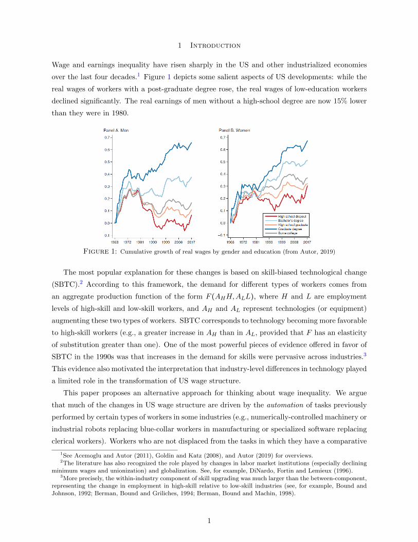
over the last four decades.1 Figure 1 depicts some salient aspects of US developments: while the

real wages of workers with a post-graduate degree rose, the real wages of low-education workers

declined significantly. The real earnings of men without a high-school degree are now 15% lower

than they were in 1980.

Figure 1: Cumulative growth of real wages by gender and education (from Autor, 2019)

The most popular explanation for these changes is based on skill-biased technological change

(SBTC).2 According to this framework, the demand for different types of workers comes from

an aggregate production function of the form F (AHH,ALL), where H and L are employment

levels of high-skill and low-skill workers, and AH and AL represent technologies (or equipment)

augmenting these two types of workers. SBTC corresponds to technology becoming more favorable

to high-skill workers (e.g., a greater increase in AH than in AL, provided that F has an elasticity

of substitution greater than one). One of the most powerful pieces of evidence offered in favor of

SBTC in the 1990s was that increases in the demand for skills were pervasive across industries.3

This evidence also motivated the interpretation that industry-level differences in technology played

a limited role in the transformation of US wage structure.

This paper proposes an alternative approach for thinking about wage inequality. We argue

that much of the changes in US wage structure are driven by the automation of tasks previously

performed by certain types of workers in some industries (e.g., numerically-controlled machinery or

industrial robots replacing blue-collar workers in manufacturing or specialized software replacing

clerical workers). Workers who are not displaced from the tasks in which they have a comparative

1See Acemoglu and Autor (2011), Goldin and Katz (2008), and Autor (2019) for overviews.2The literature has also recognized the role played by changes in labor market institutions (especially declining

minimum wages and unionization) and globalization. See, for example, DiNardo, Fortin and Lemieux (1996).3More precisely, the within-industry component of skill upgrading was much larger than the between-component,

representing the change in employment in high-skill relative to low-skill industries (see, for example, Bound andJohnson, 1992; Berman, Bound and Griliches, 1994; Berman, Bound and Machin, 1998).

1

advantage, such as those with a postgraduate degree or women with a college degree, enjoyed

real wage gains, while those, including low-education men, who used to specialize in tasks and

industries undergoing rapid automation, experienced stagnant or declining real wages.

-20%

0

20%

40%

60%

Chan

ge in

hour

ly wa

ges,

1980

-201

6

-5 0 5 10 15 20 25 30 35Exposure to industries with

declining labor shares (in %)

A. Role of specialization across industries

-20%

0

20%

40%

60%

-5 0 5 10 15 20 25 30 35Exposure to routine jobs in industries

with declining labor shares (in %)

B. Accounting for relative specialization in routine jobs

β = −2.5

βR = −1.3

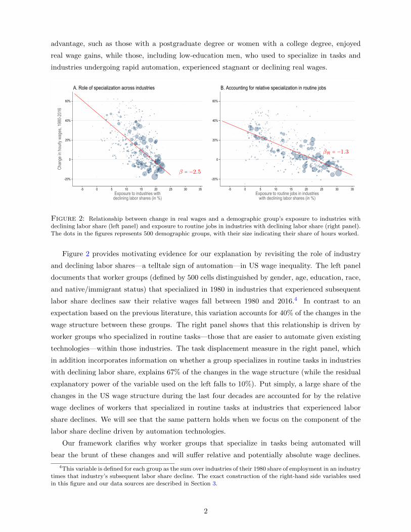
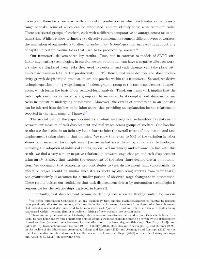
Figure 2: Relationship between change in real wages and a demographic group’s exposure to industries withdeclining labor share (left panel) and exposure to routine jobs in industries with declining labor share (right panel).The dots in the figures represents 500 demographic groups, with their size indicating their share of hours worked.

Figure 2 provides motivating evidence for our explanation by revisiting the role of industry

and declining labor shares—a telltale sign of automation—in US wage inequality. The left panel

documents that worker groups (defined by 500 cells distinguished by gender, age, education, race,

and native/immigrant status) that specialized in 1980 in industries that experienced subsequent

labor share declines saw their relative wages fall between 1980 and 2016.4 In contrast to an

expectation based on the previous literature, this variation accounts for 40% of the changes in the

wage structure between these groups. The right panel shows that this relationship is driven by

worker groups who specialized in routine tasks—those that are easier to automate given existing

technologies—within those industries. The task displacement measure in the right panel, which

in addition incorporates information on whether a group specializes in routine tasks in industries

with declining labor share, explains 67% of the changes in the wage structure (while the residual

explanatory power of the variable used on the left falls to 10%). Put simply, a large share of the

changes in the US wage structure during the last four decades are accounted for by the relative

wage declines of workers that specialized in routine tasks at industries that experienced labor

share declines. We will see that the same pattern holds when we focus on the component of the

labor share decline driven by automation technologies.

Our framework clarifies why worker groups that specialize in tasks being automated will

bear the brunt of these changes and will suffer relative and potentially absolute wage declines.

4This variable is defined for each group as the sum over industries of their 1980 share of employment in an industrytimes that industry’s subsequent labor share decline. The exact construction of the right-hand side variables usedin this figure and our data sources are described in Section 3.

2

To explain these facts, we start with a model of production in which each industry performs a

range of tasks, some of which can be automated, and we identify these with “routine” tasks.

There are several groups of workers, each with a different comparative advantage across tasks and

industries. While we allow technology to directly complement/augment different types of workers,

the innovation of our model is to allow for automation technologies that increase the productivity

of capital in certain routine tasks that used to be produced by workers.5

Our framework delivers three key results. First, and in contrast to models of SBTC with

factor-augmenting technologies, in our framework automation can have a negative effect on work-

ers who are displaced from tasks they used to perform, and such changes can take place with

limited increases in total factor productivity (TFP). Hence, real wage declines and slow produc-

tivity growth despite rapid automation are not puzzles within this framework. Second, we derive

a simple equation linking wage changes of a demographic group to the task displacement it experi-

ences, which forms the basis of our reduced-form analysis. Third, our framework implies that the

task displacement experienced by a group can be measured by its employment share in routine

tasks in industries undergoing automation. Moreover, the extent of automation in an industry

can be inferred from declines in its labor share, thus providing an explanation for the relationship

reported in the right panel of Figure 2.6

The second part of the paper documents a robust and negative (reduced-form) relationship

between our measure of task displacement and real wages across groups of workers. Our baseline

results use the decline in an industry labor share to infer the overall extent of automation and task

displacement taking place in that industry. We show that close to 50% of the variation in labor

shares (and measured task displacement) across industries is driven by automation technologies,

including the adoption of industrial robots, specialized machinery and software. In line with this

result, we find a very similar negative relationship between wage changes and task displacement

using an IV strategy that exploits the component of the labor share decline driven by automa-

tion. We document that offshoring also contributes to task displacement (and conceptually, its

effects on wages should be similar since it also works by displacing workers from their tasks),

but quantitatively it accounts for a smaller portion of observed wage changes than automation.

These results bolster our confidence that task displacement driven by automation technologies is

responsible for the relationships depicted in Figure 2.

Importantly, task displacement retains its defining role when we flexibly control for various

5We define automation technologies as any technology that enables machines/algorithms/capital to performtasks previously allocated to humans, which results in the displacement of workers from these tasks. Note, however,that task displacement does not need to be associated with “job loss”, and can take the form of a worker beingreallocated within the same firm or a decline in hiring of new workers into certain tasks.

6 There are many determinants of industry labor shares and we discuss them and explore their effects later. It isuseful to note here that we find a significant portion of industry labor share declines to be driven by the displacementof workers from (routine) tasks because of automation (and to a lesser degree offshoring). See Elsby, Hobijn andSahin (2013), Karabarbounis and Neiman (2013), Piketty (2014), Dao, Das and Koczan (2019), and Hubmer (2020)on the decline of the labor share; Acemoglu, Lelarge and Restrepo (2020) and Acemoglu and Restrepo (2020) on therole of automation in labor share declines; De Loecker, Eeckhout and Unger (2020) on the role of rising markups;and Autor et al. (2020) on superstar firms.

3

forms of SBTC (for example, allowing the productivity of workers to evolve as a function of their

education levels over time). Our estimates indicate that task displacement explains 50%–70% of

the observed changes in wage structure between 1980 and 2016, while these traditional SBTC

proxies account for less than 10%. Furthermore, the relationship between task displacement and

real wages remains unchanged when we control for other potential determinants of industry labor

shares and wages, such as rising concentration, markups, import competition and the decline

of unions, or when we exploit regional variation in specialization patterns or focus on different

sub-periods. Consistent with the notion that these trends reflect changes in labor demand, we

also estimate negative effects on employment outcomes.

Although our reduced-form analysis documents a strong negative relationship between task

displacement and relative wage changes across worker groups, it misses three indirect effects

affecting real wages in general equilibrium. First, in our regressions, the common effect of pro-

ductivity increases on real wages goes into the intercept, and so our results are not informative

about real wage level changes. Second, because automation and task displacement concentrate in

a handful of industries, they will change the sectoral composition of the economy, which can in

turn shift the demand for different types of workers. Third, our reduced-form evidence focuses on

the direct effects of task displacement, but does not account for ripple effects, which result from

displaced workers competing against others for non-automated tasks, bidding down their wages

and spreading negative wage effects of automation more broadly in the population.

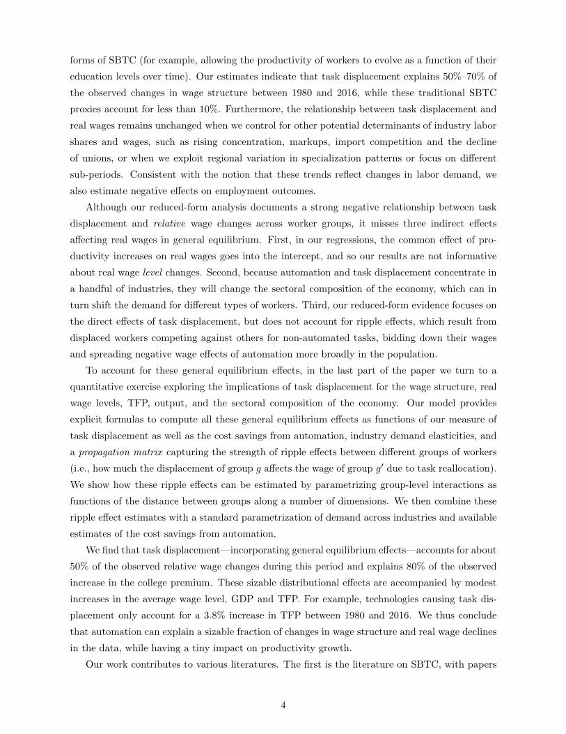
To account for these general equilibrium effects, in the last part of the paper we turn to a

quantitative exercise exploring the implications of task displacement for the wage structure, real

wage levels, TFP, output, and the sectoral composition of the economy. Our model provides

explicit formulas to compute all these general equilibrium effects as functions of our measure of

task displacement as well as the cost savings from automation, industry demand elasticities, and

a propagation matrix capturing the strength of ripple effects between different groups of workers

(i.e., how much the displacement of group g affects the wage of group g′ due to task reallocation).

We show how these ripple effects can be estimated by parametrizing group-level interactions as

functions of the distance between groups along a number of dimensions. We then combine these

ripple effect estimates with a standard parametrization of demand across industries and available

estimates of the cost savings from automation.

We find that task displacement—incorporating general equilibrium effects—accounts for about

50% of the observed relative wage changes during this period and explains 80% of the observed

increase in the college premium. These sizable distributional effects are accompanied by modest

increases in the average wage level, GDP and TFP. For example, technologies causing task dis-

placement only account for a 3.8% increase in TFP between 1980 and 2016. We thus conclude

that automation can explain a sizable fraction of changes in wage structure and real wage declines

in the data, while having a tiny impact on productivity growth.

Our work contributes to various literatures. The first is the literature on SBTC, with papers

4

such as Bound and Johnson (1992), Katz and Murphy (1992) and Card and Lemieux (2001) that

explored the evolution of between-group wage inequality in response to changes in factor supplies

and technologies augmenting the productivity of educated workers. We differ from this literature

because of our distinct conceptual framework and focus on task displacement as the main driving

force of changes in wage structure.

The second is the literature exploring the effects of lower equipment and computer prices

on wage inequality through capital-skill complementarity. This literature goes back to Griliches

(1969), and its implications for US wage inequality have been explored in Krusell et al. (2000).

Relatedly, Krueger (1993) and Autor, Katz and Krueger (1998) emphasized the role of the com-

plementarity between computers and skills. More recently, Burstein, Morales and Vogel (2019)

quantify the effects of lower computer prices on inequality in a model where skilled workers have

a comparative advantage in using computers. These papers quantify the effects of lower cap-

ital prices on inequality by assuming that capital directly complements skilled workers. Our

framework complements this work by underscoring the role of task displacement as a separate

mechanism contributing to wage inequality. We also clarify the distinction between automation

and the capital-skill complementarity studied in this literature. Notably, we show that automation

has a powerful impact on inequality even if there are no direct capital-skill complementarities.

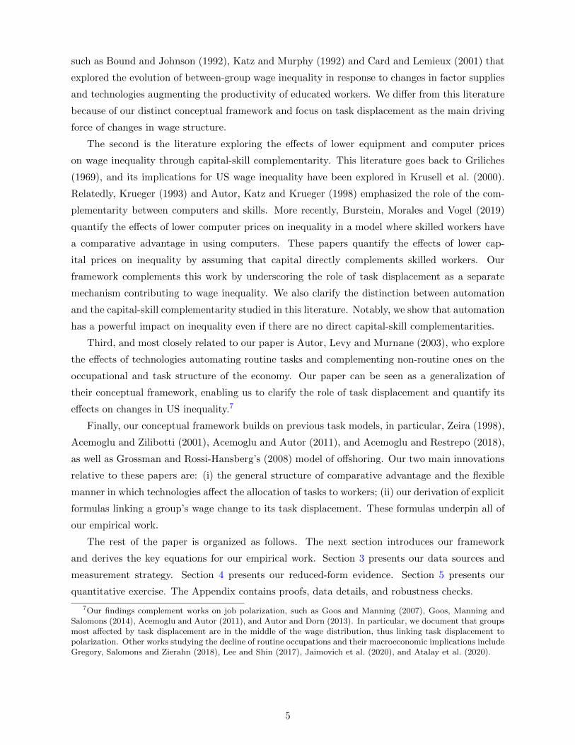
Third, and most closely related to our paper is Autor, Levy and Murnane (2003), who explore

the effects of technologies automating routine tasks and complementing non-routine ones on the

occupational and task structure of the economy. Our paper can be seen as a generalization of

their conceptual framework, enabling us to clarify the role of task displacement and quantify its

effects on changes in US inequality.7

Finally, our conceptual framework builds on previous task models, in particular, Zeira (1998),

Acemoglu and Zilibotti (2001), Acemoglu and Autor (2011), and Acemoglu and Restrepo (2018),

as well as Grossman and Rossi-Hansberg’s (2008) model of offshoring. Our two main innovations

relative to these papers are: (i) the general structure of comparative advantage and the flexible

manner in which technologies affect the allocation of tasks to workers; (ii) our derivation of explicit

formulas linking a group’s wage change to its task displacement. These formulas underpin all of

our empirical work.

The rest of the paper is organized as follows. The next section introduces our framework

and derives the key equations for our empirical work. Section 3 presents our data sources and

measurement strategy. Section 4 presents our reduced-form evidence. Section 5 presents our

quantitative exercise. The Appendix contains proofs, data details, and robustness checks.

7Our findings complement works on job polarization, such as Goos and Manning (2007), Goos, Manning andSalomons (2014), Acemoglu and Autor (2011), and Autor and Dorn (2013). In particular, we document that groupsmost affected by task displacement are in the middle of the wage distribution, thus linking task displacement topolarization. Other works studying the decline of routine occupations and their macroeconomic implications includeGregory, Salomons and Zierahn (2018), Lee and Shin (2017), Jaimovich et al. (2020), and Atalay et al. (2020).

5

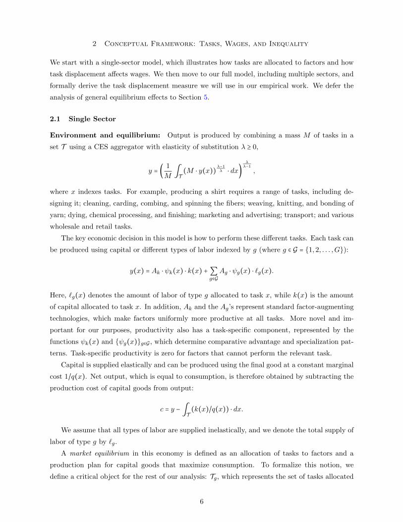
2 Conceptual Framework: Tasks, Wages, and Inequality

We start with a single-sector model, which illustrates how tasks are allocated to factors and how

task displacement affects wages. We then move to our full model, including multiple sectors, and

formally derive the task displacement measure we will use in our empirical work. We defer the

analysis of general equilibrium effects to Section 5.

2.1 Single Sector

Environment and equilibrium: Output is produced by combining a mass M of tasks in a

set T using a CES aggregator with elasticity of substitution λ ≥ 0,

y = (1

M∫T(M ⋅ y(x))

λ−1λ ⋅ dx)

λλ−1

,

where x indexes tasks. For example, producing a shirt requires a range of tasks, including de-

signing it; cleaning, carding, combing, and spinning the fibers; weaving, knitting, and bonding of

yarn; dying, chemical processing, and finishing; marketing and advertising; transport; and various

wholesale and retail tasks.

The key economic decision in this model is how to perform these different tasks. Each task can

be produced using capital or different types of labor indexed by g (where g ∈ G = {1,2, . . . ,G}):

y(x) = Ak ⋅ ψk(x) ⋅ k(x) +∑g∈G

Ag ⋅ ψg(x) ⋅ `g(x).

Here, `g(x) denotes the amount of labor of type g allocated to task x, while k(x) is the amount

of capital allocated to task x. In addition, Ak and the Ag’s represent standard factor-augmenting

technologies, which make factors uniformly more productive at all tasks. More novel and im-

portant for our purposes, productivity also has a task-specific component, represented by the

functions ψk(x) and {ψg(x)}g∈G , which determine comparative advantage and specialization pat-

terns. Task-specific productivity is zero for factors that cannot perform the relevant task.

Capital is supplied elastically and can be produced using the final good at a constant marginal

cost 1/q(x). Net output, which is equal to consumption, is therefore obtained by subtracting the

production cost of capital goods from output:

c = y − ∫T(k(x)/q(x)) ⋅ dx.

We assume that all types of labor are supplied inelastically, and we denote the total supply of

labor of type g by `g.

A market equilibrium in this economy is defined as an allocation of tasks to factors and a

production plan for capital goods that maximize consumption. To formalize this notion, we

define a critical object for the rest of our analysis: Tg, which represents the set of tasks allocated

6

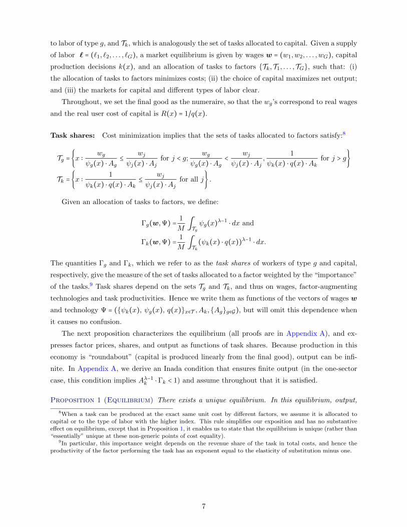
to labor of type g, and Tk, which is analogously the set of tasks allocated to capital. Given a supply

of labor ` = (`1, `2, . . . , `G), a market equilibrium is given by wages w = (w1,w2, . . . ,wG), capital

production decisions k(x), and an allocation of tasks to factors {Tk,T1, . . . ,TG}, such that: (i)

the allocation of tasks to factors minimizes costs; (ii) the choice of capital maximizes net output;

and (iii) the markets for capital and different types of labor clear.

Throughout, we set the final good as the numeraire, so that the wg’s correspond to real wages

and the real user cost of capital is R(x) = 1/q(x).

Task shares: Cost minimization implies that the sets of tasks allocated to factors satisfy:8

Tg ={x ∶wg

ψg(x) ⋅Ag≤

wj

ψj(x) ⋅Ajfor j < g;

wg

ψg(x) ⋅Ag<

wj

ψj(x) ⋅Aj,

1

ψk(x) ⋅ q(x) ⋅Akfor j > g}

Tk ={x ∶1

ψk(x) ⋅ q(x) ⋅Ak≤

wj

ψj(x) ⋅Ajfor all j} .

Given an allocation of tasks to factors, we define:

Γg(w,Ψ) =1

M∫Tg

ψg(x)λ−1

⋅ dx and

Γk(w,Ψ) =1

M∫Tk

(ψk(x) ⋅ q(x))λ−1

⋅ dx.

The quantities Γg and Γk, which we refer to as the task shares of workers of type g and capital,

respectively, give the measure of the set of tasks allocated to a factor weighted by the “importance”

of the tasks.9 Task shares depend on the sets Tg and Tk, and thus on wages, factor-augmenting

technologies and task productivities. Hence we write them as functions of the vectors of wages w

and technology Ψ = ({ψk(x), ψg(x), q(x)}x∈T ,Ak,{Ag}g∈G), but will omit this dependence when

it causes no confusion.

The next proposition characterizes the equilibrium (all proofs are in Appendix A), and ex-

presses factor prices, shares, and output as functions of task shares. Because production in this

economy is “roundabout” (capital is produced linearly from the final good), output can be infi-

nite. In Appendix A, we derive an Inada condition that ensures finite output (in the one-sector

case, this condition implies Aλ−1k ⋅ Γk < 1) and assume throughout that it is satisfied.

Proposition 1 (Equilibrium) There exists a unique equilibrium. In this equilibrium, output,

8When a task can be produced at the exact same unit cost by different factors, we assume it is allocated tocapital or to the type of labor with the higher index. This rule simplifies our exposition and has no substantiveeffect on equilibrium, except that in Proposition 1, it enables us to state that the equilibrium is unique (rather than“essentially” unique at these non-generic points of cost equality).

9In particular, this importance weight depends on the revenue share of the task in total costs, and hence theproductivity of the factor performing the task has an exponent equal to the elasticity of substitution minus one.

7

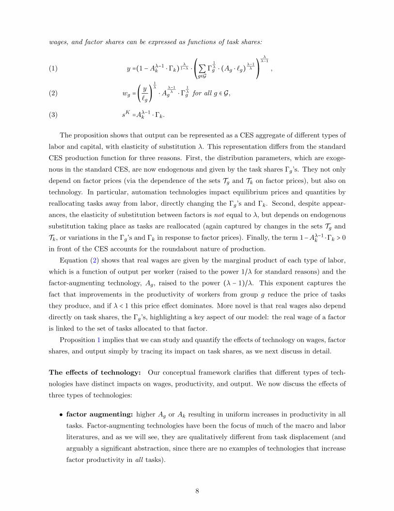
wages, and factor shares can be expressed as functions of task shares:

y =(1 −Aλ−1k ⋅ Γk)

λ1−λ ⋅

⎛

⎝∑g∈G

Γ1λg ⋅ (Ag ⋅ `g)

λ−1λ

⎞

⎠

λλ−1

,(1)

wg =(y

`g)

1λ

⋅Aλ−1λg ⋅ Γ

1λg for all g ∈ G,(2)

sK =Aλ−1k ⋅ Γk.(3)

The proposition shows that output can be represented as a CES aggregate of different types of

labor and capital, with elasticity of substitution λ. This representation differs from the standard

CES production function for three reasons. First, the distribution parameters, which are exoge-

nous in the standard CES, are now endogenous and given by the task shares Γg’s. They not only

depend on factor prices (via the dependence of the sets Tg and Tk on factor prices), but also on

technology. In particular, automation technologies impact equilibrium prices and quantities by

reallocating tasks away from labor, directly changing the Γg’s and Γk. Second, despite appear-

ances, the elasticity of substitution between factors is not equal to λ, but depends on endogenous

substitution taking place as tasks are reallocated (again captured by changes in the sets Tg and

Tk, or variations in the Γg’s and Γk in response to factor prices). Finally, the term 1−Aλ−1k ⋅Γk > 0

in front of the CES accounts for the roundabout nature of production.

Equation (2) shows that real wages are given by the marginal product of each type of labor,

which is a function of output per worker (raised to the power 1/λ for standard reasons) and the

factor-augmenting technology, Ag, raised to the power (λ − 1)/λ. This exponent captures the

fact that improvements in the productivity of workers from group g reduce the price of tasks

they produce, and if λ < 1 this price effect dominates. More novel is that real wages also depend

directly on task shares, the Γg’s, highlighting a key aspect of our model: the real wage of a factor

is linked to the set of tasks allocated to that factor.

Proposition 1 implies that we can study and quantify the effects of technology on wages, factor

shares, and output simply by tracing its impact on task shares, as we next discuss in detail.

The effects of technology: Our conceptual framework clarifies that different types of tech-

nologies have distinct impacts on wages, productivity, and output. We now discuss the effects of

three types of technologies:

• factor augmenting: higher Ag or Ak resulting in uniform increases in productivity in all

tasks. Factor-augmenting technologies have been the focus of much of the macro and labor

literatures, and as we will see, they are qualitatively different from task displacement (and

arguably a significant abstraction, since there are no examples of technologies that increase

factor productivity in all tasks).

8

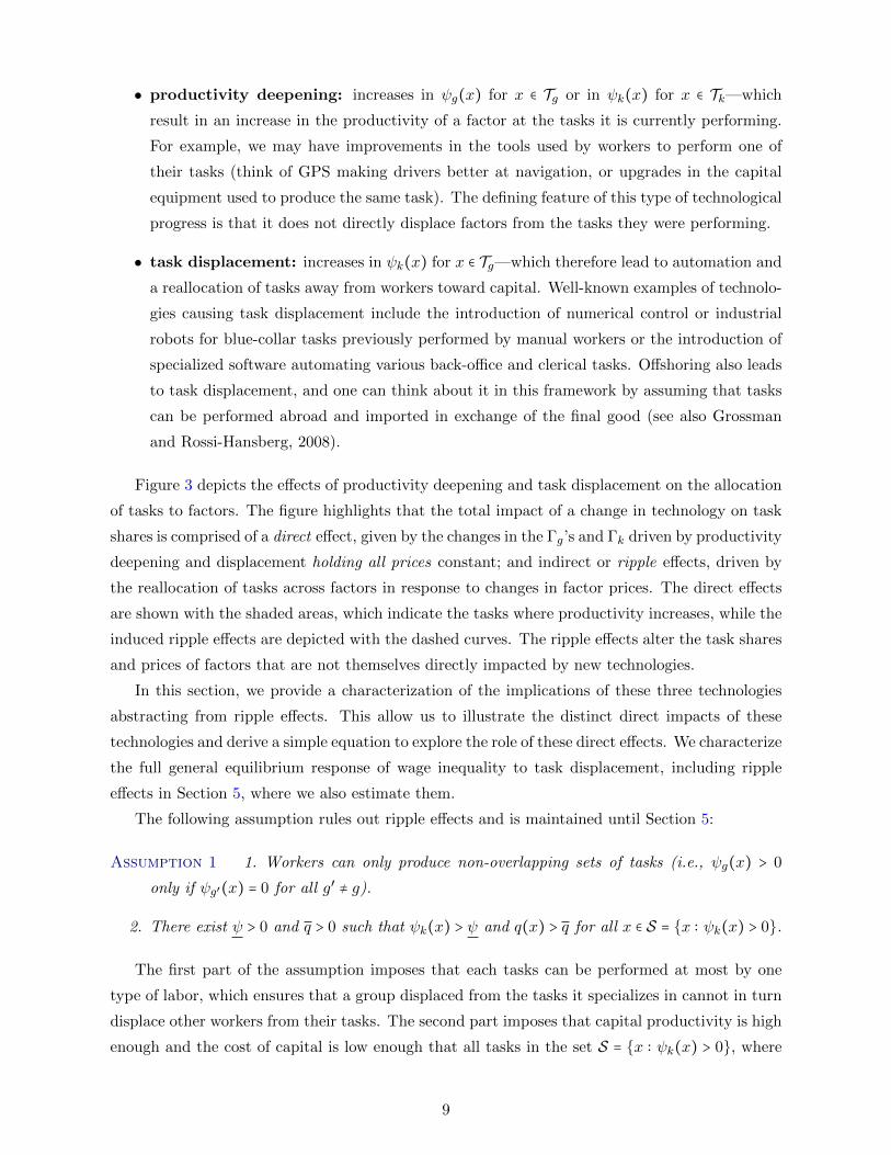
• productivity deepening: increases in ψg(x) for x ∈ Tg or in ψk(x) for x ∈ Tk—which

result in an increase in the productivity of a factor at the tasks it is currently performing.

For example, we may have improvements in the tools used by workers to perform one of

their tasks (think of GPS making drivers better at navigation, or upgrades in the capital

equipment used to produce the same task). The defining feature of this type of technological

progress is that it does not directly displace factors from the tasks they were performing.

• task displacement: increases in ψk(x) for x ∈ Tg—which therefore lead to automation and

a reallocation of tasks away from workers toward capital. Well-known examples of technolo-

gies causing task displacement include the introduction of numerical control or industrial

robots for blue-collar tasks previously performed by manual workers or the introduction of

specialized software automating various back-office and clerical tasks. Offshoring also leads

to task displacement, and one can think about it in this framework by assuming that tasks

can be performed abroad and imported in exchange of the final good (see also Grossman

and Rossi-Hansberg, 2008).

Figure 3 depicts the effects of productivity deepening and task displacement on the allocation

of tasks to factors. The figure highlights that the total impact of a change in technology on task

shares is comprised of a direct effect, given by the changes in the Γg’s and Γk driven by productivity

deepening and displacement holding all prices constant; and indirect or ripple effects, driven by

the reallocation of tasks across factors in response to changes in factor prices. The direct effects

are shown with the shaded areas, which indicate the tasks where productivity increases, while the

induced ripple effects are depicted with the dashed curves. The ripple effects alter the task shares

and prices of factors that are not themselves directly impacted by new technologies.

In this section, we provide a characterization of the implications of these three technologies

abstracting from ripple effects. This allow us to illustrate the distinct direct impacts of these

technologies and derive a simple equation to explore the role of these direct effects. We characterize

the full general equilibrium response of wage inequality to task displacement, including ripple

effects in Section 5, where we also estimate them.

The following assumption rules out ripple effects and is maintained until Section 5:

Assumption 1 1. Workers can only produce non-overlapping sets of tasks (i.e., ψg(x) > 0

only if ψg′(x) = 0 for all g′ ≠ g).

2. There exist ψ > 0 and q > 0 such that ψk(x) > ψ and q(x) > q for all x ∈ S = {x ∶ ψk(x) > 0}.

The first part of the assumption imposes that each tasks can be performed at most by one

type of labor, which ensures that a group displaced from the tasks it specializes in cannot in turn

displace other workers from their tasks. The second part imposes that capital productivity is high

enough and the cost of capital is low enough that all tasks in the set S = {x ∶ ψk(x) > 0}, where

9

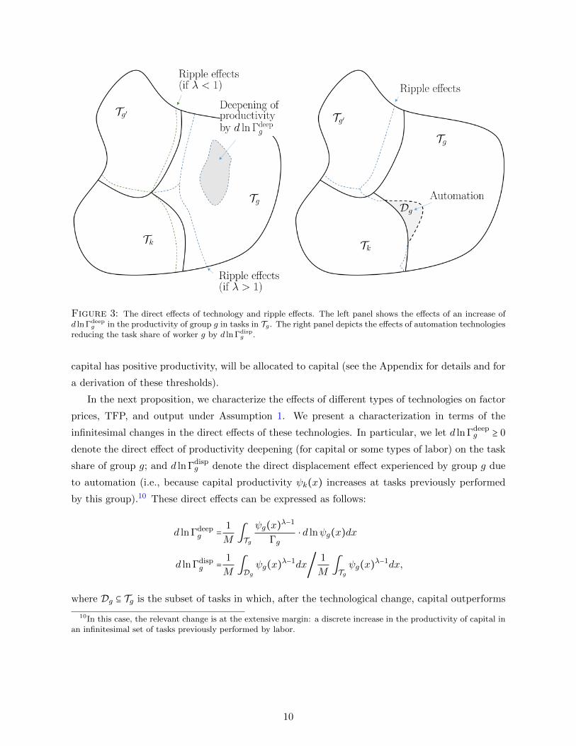
Figure 3: The direct effects of technology and ripple effects. The left panel shows the effects of an increase ofd ln Γdeep

g in the productivity of group g in tasks in Tg. The right panel depicts the effects of automation technologiesreducing the task share of worker g by d ln Γdisp

g .

capital has positive productivity, will be allocated to capital (see the Appendix for details and for

a derivation of these thresholds).

In the next proposition, we characterize the effects of different types of technologies on factor

prices, TFP, and output under Assumption 1. We present a characterization in terms of the

infinitesimal changes in the direct effects of these technologies. In particular, we let d ln Γdeepg ≥ 0

denote the direct effect of productivity deepening (for capital or some types of labor) on the task

share of group g; and d ln Γdispg denote the direct displacement effect experienced by group g due

to automation (i.e., because capital productivity ψk(x) increases at tasks previously performed

by this group).10 These direct effects can be expressed as follows:

d ln Γdeepg =

1

M∫Tg

ψg(x)λ−1

Γg⋅ d lnψg(x)dx

d ln Γdispg =

1

M∫Dg

ψg(x)λ−1dx/

1

M∫Tg

ψg(x)λ−1dx,

where Dg ⊆ Tg is the subset of tasks in which, after the technological change, capital outperforms

10In this case, the relevant change is at the extensive margin: a discrete increase in the productivity of capital inan infinitesimal set of tasks previously performed by labor.

10

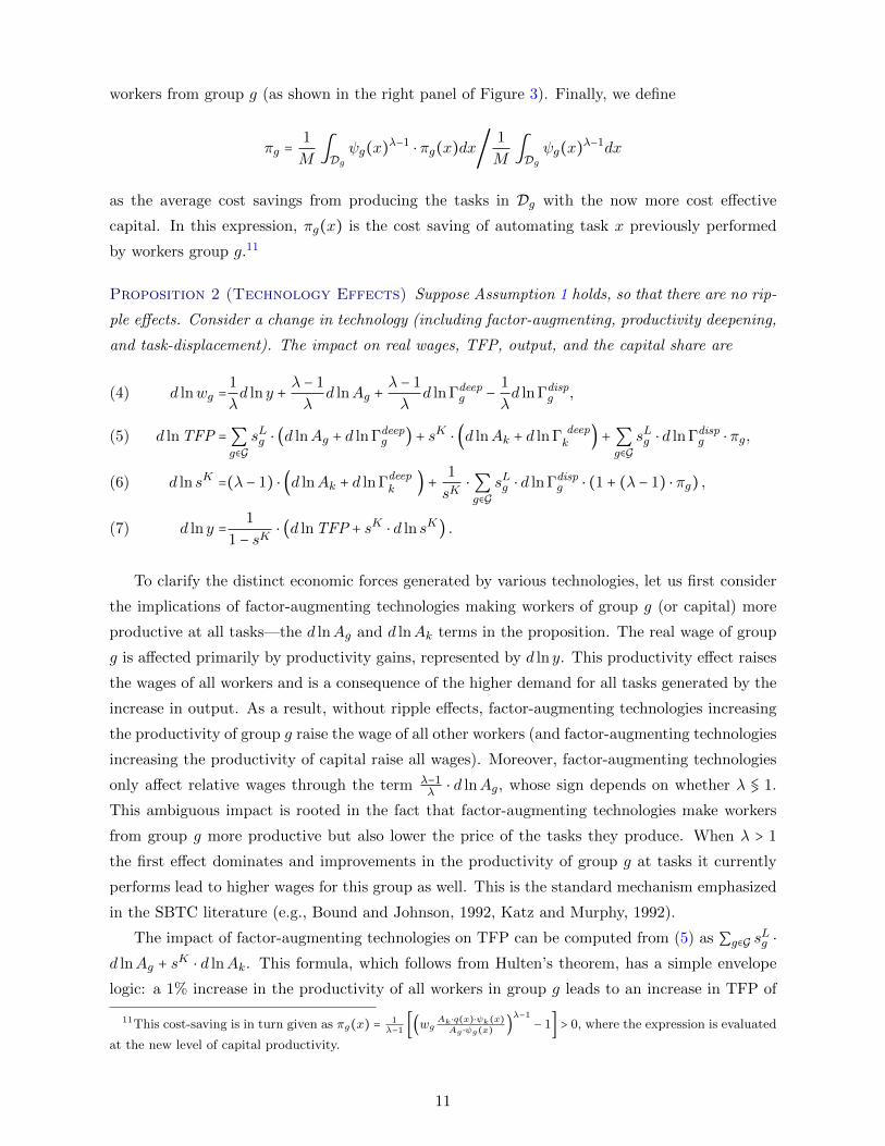
workers from group g (as shown in the right panel of Figure 3). Finally, we define

πg =1

M∫Dg

ψg(x)λ−1

⋅ πg(x)dx/1

M∫Dg

ψg(x)λ−1dx

as the average cost savings from producing the tasks in Dg with the now more cost effective

capital. In this expression, πg(x) is the cost saving of automating task x previously performed

by workers group g.11

Proposition 2 (Technology Effects) Suppose Assumption 1 holds, so that there are no rip-

ple effects. Consider a change in technology (including factor-augmenting, productivity deepening,

and task-displacement). The impact on real wages, TFP, output, and the capital share are

d lnwg =1

λd ln y +

λ − 1

λd lnAg +

λ − 1

λd ln Γdeep

g −1

λd ln Γdisp

g ,(4)

d ln TFP =∑g∈G

sLg ⋅ (d lnAg + d ln Γdeepg ) + sK ⋅ (d lnAk + d ln Γ deep

k ) +∑g∈G

sLg ⋅ d ln Γdispg ⋅ πg,(5)

d ln sK =(λ − 1) ⋅ (d lnAk + d ln Γdeepk ) +

1

sK⋅∑g∈G

sLg ⋅ d ln Γdispg ⋅ (1 + (λ − 1) ⋅ πg) ,(6)

d ln y =1

1 − sK⋅ (d ln TFP + sK ⋅ d ln sK) .(7)

To clarify the distinct economic forces generated by various technologies, let us first consider

the implications of factor-augmenting technologies making workers of group g (or capital) more

productive at all tasks—the d lnAg and d lnAk terms in the proposition. The real wage of group

g is affected primarily by productivity gains, represented by d ln y. This productivity effect raises

the wages of all workers and is a consequence of the higher demand for all tasks generated by the

increase in output. As a result, without ripple effects, factor-augmenting technologies increasing

the productivity of group g raise the wage of all other workers (and factor-augmenting technologies

increasing the productivity of capital raise all wages). Moreover, factor-augmenting technologies

only affect relative wages through the term λ−1λ ⋅ d lnAg, whose sign depends on whether λ ≶ 1.

This ambiguous impact is rooted in the fact that factor-augmenting technologies make workers

from group g more productive but also lower the price of the tasks they produce. When λ > 1

the first effect dominates and improvements in the productivity of group g at tasks it currently

performs lead to higher wages for this group as well. This is the standard mechanism emphasized

in the SBTC literature (e.g., Bound and Johnson, 1992, Katz and Murphy, 1992).

The impact of factor-augmenting technologies on TFP can be computed from (5) as ∑g∈G sLg ⋅

d lnAg + sK ⋅ d lnAk. This formula, which follows from Hulten’s theorem, has a simple envelope

logic: a 1% increase in the productivity of all workers in group g leads to an increase in TFP of

11This cost-saving is in turn given as πg(x) = 1λ−1 [(wg Ak ⋅q(x)⋅ψk(x)

Ag ⋅ψg(x))λ−1− 1] > 0, where the expression is evaluated

at the new level of capital productivity.

11

sLg %, where sLg is the share of skilled labor in GDP. Likewise, a 1% increase in the productivity of

capital at all tasks leads to an increase in TFP of sK%. Thus, relative to their modest effects on

the wage structure (especially for values of λ close to 1), factor-augmenting technologies have large

productivity effects. If factor-augmenting technologies were at the root of changes in the wage

structure, then we should see sizable TFP gains (unless there is technological regress, see Acemoglu

and Restrepo, 2019). Note finally that, with no ripple effects, factor-augmenting technologies have

identical effects as technologies generating a deepening of productivity—the terms d ln Γdeepg and

d ln Γdeepk .

These results contrast with the effects of automation, which displaces some workers from the

tasks they are performing, and whose effects are captured by the term d ln Γdispg in the proposition.

The impact of this type of technology on wages in (4) becomes 1λd ln y− 1

λd ln Γdispg . The first term

is once again the productivity effect, which raises the wages of all workers. More novel and

important for our purposes is the second term, which links wage changes to task displacement

and is negative (independently of whether λ ≶ 1). As we will see, this key insight generalizes to

our full model and forms the basis of our empirical work.

The implications of automation for TFP and factor shares are also very different from those

of factor-augmenting technologies. The change in TFP is now ∑g∈G sLg ⋅d ln Γdisp

g ⋅πg. If πg is small

for groups being displaced (meaning small productivity gains from substituting capital for labor),

then TFP growth could be arbitrarily small, even if there is considerable automation. As a result,

the displacement effect can outweigh the productivity effect and, as a result, the real wage for

displaced groups can decline despite the economy’s higher productivity.

Equation (6) also shows that task displacement always results in an increase in the capital

share and a reduction in the labor share of value added—an observation that will motivate our

measurement approach in Section 2.3. This is also in stark contrast to what one would get from

factor-augmenting technologies, whose impact on factor shares depends on whether λ ≶ 1 (with

no ripple effects, λ is also the elasticity of substitution between capital and labor).

2.2 Full Model: Multiple Sectors

Our full model generalizes the one-sector setup in the previous subsection. There are multiple

industries indexed by i ∈ I = {1,2, . . . , I}. Output in industry i is produced by combining the

tasks in some set Ti, with measure Mi, using a CES aggregator with elasticity λ ≥ 0:

yi = Ai ⋅ (1

Mi∫Ti

(Mi ⋅ y(x))λ−1λ ⋅ dx)

λλ−1

,

where x again indexes tasks and Ai is a Hicks-neutral industry productivity term. As before,

tasks, Tgi denotes the set of tasks in industry i allocated to workers of type g and Tki denotes

12

those allocated to capital. Likewise, we define industry-level task shares, Γgi and Γki, as:

Γgi(w,Ψ) =1

Mi∫Tgi

ψg(x)λ−1

⋅ dx;Γki(w,Ψ) =1

Mi∫Tki

(ψk(x) ⋅ q(x))λ−1

⋅ dx.

We assume that industry outputs are combined into a single final good using a constant returns

to scale aggregator. Rather than specifying this aggregator, we work with the implied expenditure

shares, sYi (p), where p = (p1, p2, . . . , pI) is the vector of industry prices.12

The next proposition generalizes Proposition 1 to this environment and characterizes the

equilibrium in terms of task shares.

Proposition 3 (Equilibrium in multi-sector economy) There is a unique equilibrium. In

this equilibrium, output, wages, and industry prices can be expressed as functions of task shares

defined implicitly by the solution to the system of equations:

wg =(y

`g)

1λ

⋅Aλ−1λg ⋅ (∑

i∈I

sYi (p) ⋅ (Aipi)λ−1

⋅ Γgi)

1λ

(8)

pi =1

Ai

⎛

⎝Aλ−1k ⋅ Γki +∑

g∈G

w1−λg ⋅Aλ−1

g ⋅ Γgi⎞

⎠

11−λ

(9)

1 =∑i∈I

sYi (p).(10)

The proposition shows that task shares, the Γki’s and Γgi’s, continue to be a key determinant

of real wages, and we can express the equilibrium of the economy as a function of task shares,

though we no longer have a closed-form solution for output. Moreover, the effects of automation

technologies on equilibrium outcomes again work via their impact on task shares.

2.3 Mapping the Model to Data

In this subsection, we use Proposition 3 to derive an equation that links the change in wages

to the direct effects of task displacement (and other technologies), extending (4) to this envi-

ronment. This equation will form the basis of our reduced-form analysis. We will then use our

model to derive a measure of task displacement that captures its direct effects across groups of

workers. These equations and measures will be generalized to include ripple effects in our general

equilibrium analysis in Section 5.

Task displacement and wage structure: As before, denote the effects productivity deepen-

ing and automation on task shares in industry i by d ln Γdeepgi and d ln Γdisp

gi , respectively. Differ-

12For example, a CES demand system over industries with elasticity of substitution η would imply sYi (p) = αi⋅p1−ηi .This formulation imposes homotheticity, which can be relaxed by allowing expenditure shares to also depend onthe level of consumption, but this is not central to our focus.

13

entiating equation (8) and using Assumption 1, we obtain a generalization of (4):

d lnwg =1

λd ln y +

λ − 1

λ(d lnAg +∑

i∈I

ωig ⋅ d ln Γdeepgi )(11)

+1

λ∑i∈I

ωig ⋅ (d ln sYi + (1 − λ)(d lnpi + d lnAi)) −1

λ∑i∈I

ωig ⋅ d ln Γdispgi ,

where ωig denotes the share of group g’s wage income earned in industry i, so that ∑i∈I ωig = 1.

Equation (11) shows that wages depend on four terms, which we next explain (and also outline

how they will be measured in our reduced-form empirical work):

• The common expansion of output: d ln y, which captures the productivity effect. In our

reduced-form regressions, this effect will be absorbed by the constant term.

• Group-specific shifters: λ−1λ (d lnAg +∑i∈I ω

ig ⋅ d ln Γdeep

gi ), which represent the contribution

of factor-augmenting technologies and productivity deepening. Following the SBTC litera-

ture, in our reduced-form regressions we will assume that these technologies augment certain

well-defined skills associated with education and also allow them to be gender-biased. In

particular, we parameterize these as:

λ − 1

λ(d lnAg +∑

i∈I

ωig ⋅ d ln Γdeepgi ) = αedu(g) + γgender(g) + υg,

where υg is an additional unobserved component, and in our regression analysis, they will

be absorbed by dummies for gender and education levels. As a further refinement, we allow

group-specific shifters to also depend on baseline group wages, which may proxy for skills

as well.

• Industry shifters:

Industry shifterg =1

λ∑i∈I

ωig ⋅ (d ln sYi + (1 − λ)(d lnpi + d lnAi)) ,

which capture the effects coming from the expansion or contraction of industries in which a

demographic group specializes (for example, due to trade in final goods, structural transfor-

mation, or the uneven effects of automation in some sectors). In our reduced-form regres-

sions, we control for this term by including the exposure of a group to the change in value

added of the sectors in which it specializes.

• Task displacement :

Task displacementg =∑i∈I

ωig ⋅ d ln Γdispgi .

This term represents the direct effect of task displacement on a demographic group’s wages

and will be the focus of our empirical work. As equation (11) shows, the key prediction of

14

our model is that groups exposed to taks displacement should experience a decline in their

relative wages. Unlike other technologies, this effect is always negative—independently of

whether the elasticity of substitution λ is above or below 1. Task displacement could come

from automation or offshoring, and we will later study their contribution to this process.

Measuring task displacement: We now turn to measuring task displacement. Our measure

summarizes the direct effects of task-displacing technologies on different groups of workers, and

will form the basis of our reduced-form regression analysis and quantitative evaluation.

We use two complementary strategies to measure task displacement, both of which rely on an

initial observation: task displacement takes place mainly in tasks that can be automated, which

we initially proxy with routine tasks.13 Formally, we impose the following assumption:

Assumption 2 Only routine tasks are automated and, within an industry, different groups of

workers are displaced from their routine tasks at a common rate.

The next component of our measurement requires a proxy for the extent of task displacement

taking place in each industry. Our two strategies take different approaches to this problem. Our

first strategy develops a more comprehensive measure based on the idea that task displacement

is tightly linked to declines in industry labor shares, and uses the “unexplained” portion of the

change in labor share to infer task displacement at the industry level. Specifically, and as we

show in Appendix E, when λ = 1 (so that the task aggregator is Cobb-Douglas) and there are no

changes in industry markups, we have:

Task displacementg =∑i∈I

ωig ⋅ (ωRgi/ω

Ri ) ⋅ (−d ln sLi ).(12)

This measure comprises three terms: (1) a group’s exposure to different industries, ωig, which is

given by the share of wages earned by workers of group g in industry i; (2) the percent decline

in the labor share, −d ln sLi , which in our framework is tightly linked to automation in industry

i; (3) ωRgi/ωRi , which captures the relative specialization of group g in industry i’s routine jobs,

where displacement takes place.14 The measure of task displacement in equation (12) is precisely

the one used in the right panel of Figure 2, while the left panel focuses on exposure to industries

with declining labor shares and ignores the relative specialization of workers in routine jobs.15

13The idea that routine tasks are easier to automate is the main premise of Autor, Levy and Murnane (2003) andis in line with several studies that document a decline in routine jobs following automation, including Acemogluand Restrepo (2020) and Humlum (2020). We additionally show very similar results using various other measuresof which tasks can be automated.

Although which tasks can be automated will likely change with advances in AI, AI technologies are not presentfor most of our sample. Acemoglu et al. (2020) show that AI use takes off in the US after 2015.

14Relative specialization is given by the ratio of the share of wages earned in routine jobs by workers in group gat industry i—ωRgi—to the share of wages earned in routine jobs by all workers in industry i—ωRi .

15Although we use the measure in equation (12) in most of our analysis, this formula can be extended to themore general case where λ ≠ 1 and markups change over time, and we provide robustness checks using this moregeneral formulation later in the paper.

15

Our second strategy uses direct measures of automation technologies (and offshoring):

task displacement due to automationg =∑i∈I

ωig ⋅ (ωRgi/ω

Ri ) ⋅ automation in industryi.(13)

Although these measures can be included directly on the right-hand side of our wage regressions,

we focus on specifications where they are used as instruments for the measure of task displace-

ment based on labor share declines, which enables us to compare coefficient estimates across

specifications.

These two strategies are complementary, and we present results using both throughout the

paper. While the second strategy has the advantage that it exploits actual measures of automa-

tion, such as adoption of industrial robots or specialized machinery and software, it might miss

other technologies generating task displacement. The more comprehensive measure exploiting the

unexplained decline in industry’s labor shares captures all dimensions of task displacement but

may be confounded by other economic forces impacting labor shares.

3 Data, Measurement, and Descriptive Patterns

In this section, we describe our data sources, substantiate the link between task displacement

and automation technologies, and provide a first look at the relationship between a demographic

group’s task displacement and its real wage changes.

3.1 Main Data Sources

We use data from the BEA Integrated Industry-Level Production Accounts on industry labor

shares, factor prices, and value added for 49 industries that can be tracked consistently from 1987

to 2016.16 We complement these industry data with proxies of the adoption of automation tech-

nologies, including BLS data on the change in the share of specialized machinery and software in

value added from 1987 to 2016, and measures of robot adoption by industry from the International

Namely, Appendix E shows that, more generally, a measure of task displacement correcting for changes in factorprices and markups can be constructed as:

Task displacementg =∑i∈Iωig ⋅ (ωRgi/ωRi ) ⋅ −d ln sLi + d lnµi − sKi ⋅ (1 − λ) ⋅ (d lnwi − d lnRi)

1 + (λ − 1) ⋅ sLi ⋅ πi,

where d lnµi is an estimate of the increase in markups in industry i. Put differently, rather than focusing onthe raw decline in the labor share, we now incorporate the effects of prices and markups on the labor share andfocus on the unexplained component. In addition, the term 1 + (λ − 1) ⋅ sLi ⋅ πi in the denominator adjusts for thesubstitution toward automated tasks following a cost reduction of πi—the average cost saving from automationin industry i. When computing this measure, we set πi = 30%, a choice we discuss in detail in the quantitativesection. Appendix E clarifies that this expression is an approximation because it ignores the effects of augmentingtechnologies or productivity deepening. It also shows, however, that the contribution of these terms to changes inthe labor share is small, and that the approximation is accurate.

16These 49 industries can be consistently tracked in Census data and BLS data and cover the entire non-government sector. When constructing our measures of task displacement, we assume that workers in the gov-ernment sector experience no automation or offshoring.

16

Federation of Robotics (IFR).17 In particular, we rely on the adjusted penetration of robots from

1993 to 2014 described in detail in Acemoglu and Restrepo (2020) as a measure of robot adoption

driven by international advances in technology. We also combine these measures into a single

index of automation, computed as the predicted decline in an industry’s labor share from 1987 to

2016 based on its robot adoption and utilization of software and specialized equipment (specifi-

cally, this is the predicted value of industry labor share given these three measures). In addition,

we look at a measure of changes in intermediate imports to proxy for offshoring (from Feenstra

and Hanson, 1999). Finally, to control for other trends affecting industries, we use data on sales

concentration, estimates of markups, unionization rates (from the CPS), measures of Chinese

import competition and industry TFP. These covariates are described in detail in Appendix F.

On the worker side, we use US Census and American Community Survey (ACS) data to trace

the labor market outcomes of 500 demographic groups defined by gender, education (less than

high school, high school graduate, some college, college degree, and post-graduate degree), age

(proxied by 10–year age bins, from 16–25 years to 56–65), race/ethnicity (White, Black, Asian,

Hispanic, Other), and native vs. foreign-born. For each demographic group, we measure real

hourly wages and other labor market outcomes in 1980 (using the 1980 US Census) and in 2016

(pooling data from the 2014–2018 ACS), and compute the change in real wages, employment,

and non-participation rates from 1980 to 2016. In Section 4.7, we also zero in on variation in

labor market outcomes for demographic groups across US regions and commuting zones. Further

details on these data are provided in Appendix F.

We measure task displacement for these 500 demographic groups exploiting their specialization

patterns across industries and in routine jobs from the 1980 Census—a year that predates major

advances in automation technologies. To do so, we create a consistent mapping of the 49 industries

in the BEA data to the Census industry classification, and for each industry, compute the share of

wages earned in routine jobs by a demographic group, using the definition of routine occupations

described in Acemoglu and Autor (2011). About a third of the occupations in the 1980 Census

are classified as routine according to this measure (see Appendix F).

3.2 Task Displacement and Changes in the Labor Share across Industries

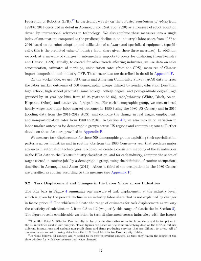
The blue bars in Figure 4 summarize our measure of task displacement at the industry level,

which is given by the percent decline in an industry labor share that is not explained by changes

in factor prices.18 The whiskers indicate the range of estimates for task displacement as we vary

the elasticity of substitution λ from 0.8 to 1.2 (we justify this range of elasticities in Section 5).

The figure reveals considerable variation in task displacement across industries, with the largest

17The BLS Total Multifactor Productivity tables provide alternative series for labor share and factor prices inthe 49 industries used in our analysis. These figures are based on the same underlying data as the BEA’s, but usedifferent imputations and exclude non-profit firms and firms producing services that are difficult to price. All ofour results are robust to using data from the BLS Total Multifactor Productivity Tables.

18In what follows, all changes are re-scaled to 36-year equivalent changes, so that they match the length of thetime window for which we measure real wage changes.

17

levels of task displacement seen in mining, chemical products, petroleum, car manufacturing,

and computers and electronics. In what follows, we focus on the measure of task displacement

computed for λ = 1 (in which case, industry-level task displacement is the same as the percent

decline in an industry’s labor share), and we use different values of λ for robustness.

-40

-20

020

4060

80

Minin

gTr

ansp

ortat

ion pi

pelin

esCh

emica

l pro

ducts

Petro

leum

and c

oal p

rodu

ctsTr

ansp

ortat

ion by

rail

Prim

ary m

etals

Tran

spor

tation

by ai

rMo

tor ve

hicles

Lega

l ser

vices

Comm

unica

tions

Nonm

etallic

mine

ral p

rodu

ctsCo

mpute

rs an

d elec

tronic

sCo

mpute

r ser

vices

Print

ing an

d pub

lishin

gW

holes

aleAc

comm

odati

onFo

od m

anufa

cturin

gTr

ansp

ortat

ion by

wate

rOt

her t

rans

porta

tion e

quipm

ent

Retai

lPl

astic

and r

ubbe

r pro

ducts

Mach

inery

Finan

ce an

d ins

uran

ceCo

nstru

ction

Tran

spor

tation

by tr

uck

Tran

spor

tation

of tr

ansit

Furn

iture

Pape

r pro

ducts

Educ

ation

al se

rvice

sTe

xtiles

Ambu

lator

y hea

lth ca

reW

ood p

rodu

ctsMi

scell

aneo

us m

anufa

cturin

gAp

plian

ces

Resta

uran

tsOi

l and

gas e

xtrac

tion

Metal

prod

ucts

Tran

spor

tation

servi

ces a

nd su

ppor

tHo

spita

lsPr

ofess

ional

servi

ces

Real

estat

eSo

cial a

ssist

ance

War

ehou

sing a

nd st

orag

eAd

minis

trativ

e ser

vices

Utilit

iesPe

rsona

l ser

vices

Recre

ation

Appa

rel a

nd Le

ather

Agric

ultur

e and

farm

ing

Task displacement and component due to observed technologies (in %), 1987-2016

Figure 4: Task displacement 1987-2016 and index of automation. The blue bars provide our baseline measureof task displacement and the whiskers give the range of estimates obtained as we vary λ from 0.8 to 1.2 , while theyellow bars show the component of task displacement explained by our index of automation. See text for variabledefinitions.

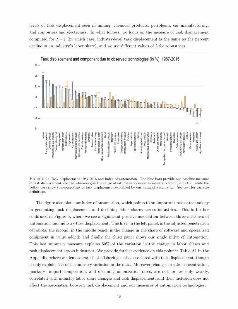
The figure also plots our index of automation, which points to an important role of technology

in generating task displacement and declining labor shares across industries. This is further

confirmed in Figure 5, where we see a significant positive association between three measures of

automation and industry task displacement. The first, in the left panel, is the adjusted penetration

of robots; the second, in the middle panel, is the change in the share of software and specialized

equipment in value added; and finally the third panel shows our single index of automation.

This last summary measure explains 50% of the variation in the change in labor shares and

task displacement across industries. We provide further evidence on this point in Table A1 in the

Appendix, where we demonstrate that offshoring is also associated with task displacement, though

it only explains 2% of the industry variation in the data. Moreover, changes in sales concentration,

markups, import competition, and declining unionization rates, are not, or are only weakly,

correlated with industry labor share changes and task displacement, and their inclusion does not

affect the association between task displacement and our measures of automation technologies.

18

ApparelAgriculture

Prof. servicesRestaurants

PlasticsRetail

Comp. services

Motor vehicles

Chemicals

Metals

-20

-10

010

2030

4050

60

0 1 2 3 4Log of one plus adjusted penetration

of robots

A. Industry task displacement (%), 1987-2016

ApparelAgriculture

Prof. servicesRestaurants

PlasticsRetail

Comp. services

Motor vehicles

Chemicals

Metals

-20

-10

010

2030

4050

60

-5 0 5 10Change in share of softwareand specialized equipment

B. Industry task displacement (%), 1987-2016

ApparelAgriculture

Prof. servicesRestaurants

PlasticsRetail

Comp. services

Motor vehicles

Chemicals

Metals

-20

-10

010

2030

4050

60

0 20 40 60Component driven

by automation

C. Industry task displacement (%), 1987-2016

Figure 5: Relationship between automation technologies and task displacement across industries. See text forvariable definitions. The five industries with the highest and lowest levels of task displacement are identified in thefigures.

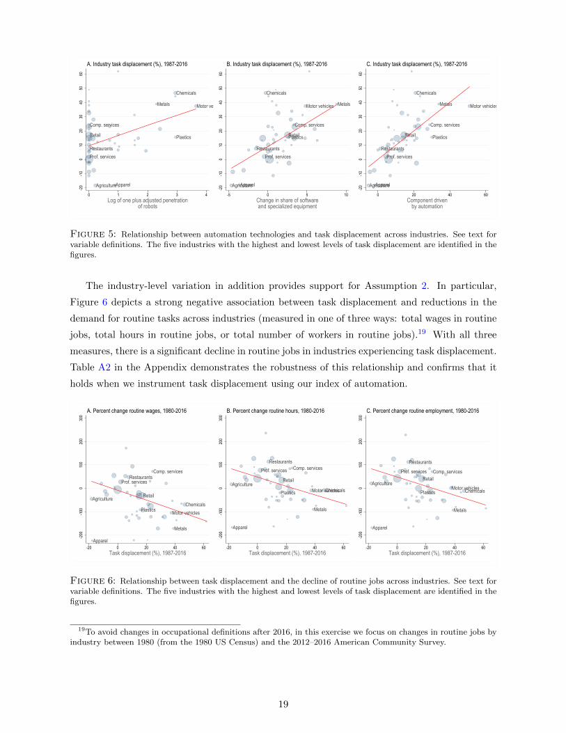
The industry-level variation in addition provides support for Assumption 2. In particular,

Figure 6 depicts a strong negative association between task displacement and reductions in the

demand for routine tasks across industries (measured in one of three ways: total wages in routine

jobs, total hours in routine jobs, or total number of workers in routine jobs).19 With all three

measures, there is a significant decline in routine jobs in industries experiencing task displacement.

Table A2 in the Appendix demonstrates the robustness of this relationship and confirms that it

holds when we instrument task displacement using our index of automation.

Agriculture

Apparel

Chemicals

Comp. services

Motor vehiclesPlastics

Metals

Prof. servicesRestaurants

Retail

-200

-100

010

020

030

0

-20 0 20 40 60Task displacement (%), 1987-2016

A. Percent change routine wages, 1980-2016

Agriculture

Apparel

Chemicals

Comp. services

Motor vehiclesPlastics

Metals

Prof. servicesRestaurants

Retail

-200

-100

010

020

030

0

-20 0 20 40 60Task displacement (%), 1987-2016

B. Percent change routine hours, 1980-2016

Agriculture

Apparel

Chemicals

Comp. services

Motor vehiclesPlastics

Metals

Prof. services

Restaurants

Retail

-200

-100

010

020

030

0

-20 0 20 40 60Task displacement (%), 1987-2016

C. Percent change routine employment, 1980-2016

Figure 6: Relationship between task displacement and the decline of routine jobs across industries. See text forvariable definitions. The five industries with the highest and lowest levels of task displacement are identified in thefigures.

19To avoid changes in occupational definitions after 2016, in this exercise we focus on changes in routine jobs byindustry between 1980 (from the 1980 US Census) and the 2012–2016 American Community Survey.

19

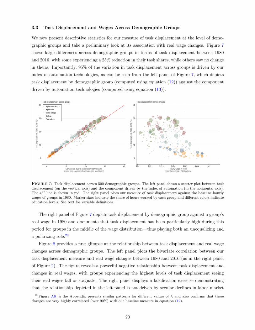
3.3 Task Displacement and Wages Across Demographic Groups

We now present descriptive statistics for our measure of task displacement at the level of demo-

graphic groups and take a preliminary look at its association with real wage changes. Figure 7

shows large differences across demographic groups in terms of task displacement between 1980

and 2016, with some experiencing a 25% reduction in their task shares, while others saw no change

in theirs. Importantly, 95% of the variation in task displacement across groups is driven by our

index of automation technologies, as can be seen from the left panel of Figure 7, which depicts

task displacement by demographic group (computed using equation (12)) against the component

driven by automation technologies (computed using equation (13)).

0

10

20

30

40

Task

disp

lacem

ent, 1

980-

2016

(%)

0 10 20 30 40Component due to automation technologies

(robots and specialized software and machinery)

Highschool dropoutHighschoolSome collegeCollegePost college

Task displacement across groups

0

10

20

30

40

Task

disp

lacem

ent, 1

980-

2016

(%)

$7.5 $10 $13.3 $17.8 $23.7 $31.6 $42Hourly wage in 1980

(logarithmic scale, 2008 dollars)

Task displacement across groups

Figure 7: Task displacement across 500 demographic groups. The left panel shows a scatter plot between taskdisplacement (on the vertical axis) and the component driven by the index of automation (in the horizontal axis).The 45○ line is shown in red. The right panel plots our measure of task displacement against the baseline hourlywages of groups in 1980. Marker sizes indicate the share of hours worked by each group and different colors indicateeducation levels. See text for variable definitions.

The right panel of Figure 7 depicts task displacement by demographic group against a group’s

real wage in 1980 and documents that task displacement has been particularly high during this

period for groups in the middle of the wage distribution—thus playing both an unequalizing and

a polarizing role.20

Figure 8 provides a first glimpse at the relationship between task displacement and real wage

changes across demographic groups. The left panel plots the bivariate correlation between our

task displacement measure and real wage changes between 1980 and 2016 (as in the right panel

of Figure 2). The figure reveals a powerful negative relationship between task displacement and

changes in real wages, with groups experiencing the highest levels of task displacement seeing

their real wages fall or stagnate. The right panel displays a falsification exercise demonstrating

that the relationship depicted in the left panel is not driven by secular declines in labor market

20Figure A6 in the Appendix presents similar patterns for different values of λ and also confirms that thesechanges are very highly correlated (over 90%) with our baseline measure in equation (12).

20

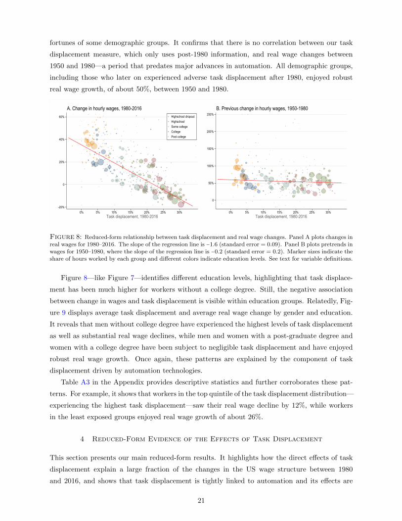
fortunes of some demographic groups. It confirms that there is no correlation between our task

displacement measure, which only uses post-1980 information, and real wage changes between

1950 and 1980—a period that predates major advances in automation. All demographic groups,

including those who later on experienced adverse task displacement after 1980, enjoyed robust

real wage growth, of about 50%, between 1950 and 1980.

-20%

0

20%

40%

60%

0% 5% 10% 15% 20% 25% 30%Task displacement, 1980-2016

Highschool dropoutHighschoolSome collegeCollegePost college

A. Change in hourly wages, 1980-2016

0

50%

100%

150%

200%

250%

0% 5% 10% 15% 20% 25% 30%Task displacement, 1980-2016

B. Previous change in hourly wages, 1950-1980

Figure 8: Reduced-form relationship between task displacement and real wage changes. Panel A plots changes inreal wages for 1980–2016. The slope of the regression line is −1.6 (standard error = 0.09). Panel B plots pretrends inwages for 1950–1980, where the slope of the regression line is −0.2 (standard error = 0.2). Marker sizes indicate theshare of hours worked by each group and different colors indicate education levels. See text for variable definitions.

Figure 8—like Figure 7—identifies different education levels, highlighting that task displace-

ment has been much higher for workers without a college degree. Still, the negative association

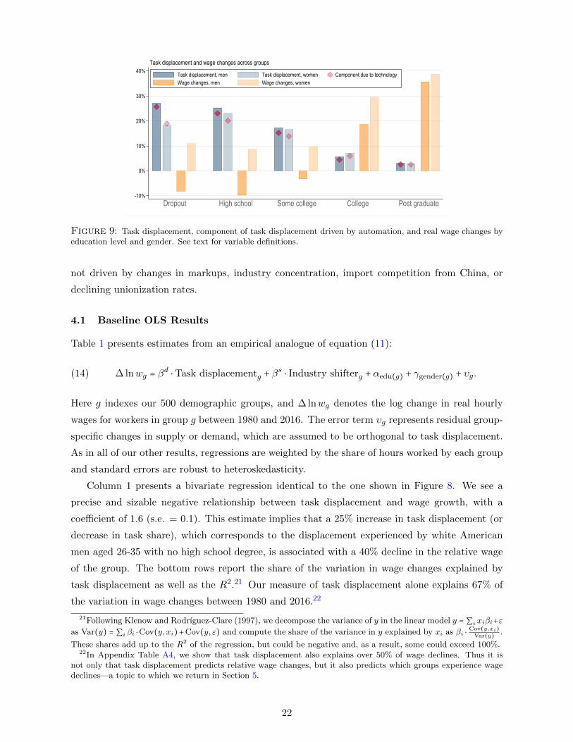
between change in wages and task displacement is visible within education groups. Relatedly, Fig-

ure 9 displays average task displacement and average real wage change by gender and education.

It reveals that men without college degree have experienced the highest levels of task displacement

as well as substantial real wage declines, while men and women with a post-graduate degree and

women with a college degree have been subject to negligible task displacement and have enjoyed

robust real wage growth. Once again, these patterns are explained by the component of task

displacement driven by automation technologies.

Table A3 in the Appendix provides descriptive statistics and further corroborates these pat-

terns. For example, it shows that workers in the top quintile of the task displacement distribution—

experiencing the highest task displacement—saw their real wage decline by 12%, while workers

in the least exposed groups enjoyed real wage growth of about 26%.

4 Reduced-Form Evidence of the Effects of Task Displacement

This section presents our main reduced-form results. It highlights how the direct effects of task

displacement explain a large fraction of the changes in the US wage structure between 1980

and 2016, and shows that task displacement is tightly linked to automation and its effects are

21

-10%

0%

10%

20%

30%

40%

Dropout High school Some college College Post graduate

Task displacement, men Task displacement, women Component due to technologyWage changes, men Wage changes, women

Task displacement and wage changes across groups

Figure 9: Task displacement, component of task displacement driven by automation, and real wage changes byeducation level and gender. See text for variable definitions.

not driven by changes in markups, industry concentration, import competition from China, or

declining unionization rates.

4.1 Baseline OLS Results

Table 1 presents estimates from an empirical analogue of equation (11):

∆ lnwg = βd⋅Task displacementg + β

s⋅ Industry shifterg + αedu(g) + γgender(g) + υg.(14)

Here g indexes our 500 demographic groups, and ∆ lnwg denotes the log change in real hourly

wages for workers in group g between 1980 and 2016. The error term υg represents residual group-

specific changes in supply or demand, which are assumed to be orthogonal to task displacement.

As in all of our other results, regressions are weighted by the share of hours worked by each group

and standard errors are robust to heteroskedasticity.

Column 1 presents a bivariate regression identical to the one shown in Figure 8. We see a

precise and sizable negative relationship between task displacement and wage growth, with a

coefficient of 1.6 (s.e. = 0.1). This estimate implies that a 25% increase in task displacement (or

decrease in task share), which corresponds to the displacement experienced by white American

men aged 26-35 with no high school degree, is associated with a 40% decline in the relative wage

of the group. The bottom rows report the share of the variation in wage changes explained by

task displacement as well as the R2.21 Our measure of task displacement alone explains 67% of

the variation in wage changes between 1980 and 2016.22

21Following Klenow and Rodrıguez-Clare (1997), we decompose the variance of y in the linear model y = ∑i xiβi+εas Var(y) = ∑i βi ⋅Cov(y, xi)+Cov(y, ε) and compute the share of the variance in y explained by xi as βi ⋅ Cov(y,xi)

Var(y) .

These shares add up to the R2 of the regression, but could be negative and, as a result, some could exceed 100%.22In Appendix Table A4, we show that task displacement also explains over 50% of wage declines. Thus it is

not only that task displacement predicts relative wage changes, but it also predicts which groups experience wagedeclines—a topic to which we return in Section 5.

22

The rest of the table documents that this bivariate relationship is robust. Column 2 controls

for industry shifters, which absorb labor demand changes coming from the expansion of industries

in which a demographic group specializes. The coefficient estimate for task displacement is similar

to the one in column 1, -1.32 (s.e. =0.16). Column 3, which we take as our baseline specification

for the rest of the paper, controls for gender and education dummies and a group’s exposure to

manufacturing, thus accounting for other demand factors favoring highly-educated workers and

for the secular decline of manufacturing. The coefficient estimate remains very similar to column

2, -1.31 (s.e. = 0.19). Even after the inclusion of these controls, task displacement still explains

55% of the variation in wage changes during this period.

Our task displacement measure combines industry-level changes in labor shares with the dis-

tribution of employment of workers across industries and occupations (where occupations are

classified into routine and non-routine). Column 4 includes two more variables, corresponding to

the constituent parts making up our task displacement measure. The first is the same variable

as the one we considered in the left panel of Figure 2 in the Introduction: the exposure of a

demographic group to industry-level declines in the labor share, but without focusing on whether

employment is in routine or non-routine tasks in that industry. The second is a group’s rela-

tive specialization in routine jobs, but this time without exploiting industry-level changes in task

displacement.23 Column 4 shows that these two variables themselves do not explain real wage

changes (conditional on task displacement and covariates), while our measure of task displace-

ment remains negatively associated with wage changes. This result confirms that our measure of

task displacement is not confounded by other industry-level changes potentially impacting labor

shares and wages or by other trends affecting workers specializing in routine tasks. Rather, it

is demographic groups specializing in routine tasks in industries undergoing sizable labor share

declines that suffer (relative) wage declines.

4.2 Baseline IV results

We now exploit information on measures of automation and offshoring to instrument for task

displacement (constructed from industry labor share declines). This strategy thus focuses on the

component of task displacement driven by automation technologies. Table 2 presents our findings.

Panel A shows the reduced-form relationship between real wage changes and the automation

measure in equation (13), focusing on our baseline specification from column 3 in Table 1.

Column 1 uses the adjusted penetration of robots from Acemoglu and Restrepo (2020). In-

dustrial robotics is an archetypal example of automation technology, but is relevant mostly in the

23Formally, these controls are defined as

exposure to industry labor share declines =∑i∈Iωig ⋅ (−d ln sLi )

relative specialization in routine jobs =∑i∈Iωig ⋅

ωRgi

ωRi.

23

good-producing sectors, thus leaving out non-robotics, software-based automation taking place

in other sectors. Columns 2 and 3 focus on, respectively, specialized machinery and software as

proxies for automation. Columns 4 and 5 include the software measure together with the other

two measures, while column 6 uses the index of automation constructed from all three variables.

In all six specifications, we see a sizable effect of these variables on real wages. For example, the

share of the variation in wage changes explained by our automation index in column 6 is of 52%

(as compared to 55% for our task displacement measure in column3 of Table 1).

In column 7, we turn to offshoring, measured as the share of imported intermediates in an

industry. As expected, offshoring also contributes to task displacement and depresses real wages of

exposed groups, but it only explains 9% of the variation in wage changes. The results in columns

6 and 7 form the basis for our claim that the bulk of the variation in task displacement is driven

by automation technologies, with a smaller contribution from offshoring.

Panel B presents our IV estimates, again focusing on the specification from column 3 of

Table 1. In each column, the variables indicated at the heading are used as instrument for the

measure of task displacement from equation (12). Across columns 1-6, the first-stage F -statistic

is quite high, ranging from 44 to 2,357, indicating that cross-industry differences in automation

provide a powerful source of variation in task displacement. The IV estimates are broadly similar

to the OLS in Table 1. For example, in column 6, where we use the automation index, task

displacement has a coefficient of -1.28 with a standard error of 0.19. The models in columns 4 and

5, where we have multiple instruments, pass the Hansen over-identification test, which bolsters

our presumption that these measures are impacting wages via the same economic channel—the

effects of automation technologies working through task displacement.

Finally, Panel C probes the robustness of our IV estimates by focusing on the specification

from column 4 of Table 1, where we also control for exposure to industry labor share declines

(also instrumented using our measures of automation) and relative specialization in routine jobs,

which is treated as exogenous. The results are similar to those in Panel B, even if somewhat less

precise. In column 6, for example, the IV estimate is -1.68 (s.e. = 0.47).

4.3 Task Displacement versus SBTC

How important is task displacement relative to other forms of SBTC? Table 3 explores this

question by considering different specifications of SBTC. The first column of this table regresses

wage changes on a full set of dummies for gender and education levels, but excludes our task

displacement measure. As explained in Section 2.3, these controls absorb any factor-augmenting

productivity trends common to all workers with the same education level or gender.24 Column

1 shows that without controlling for task displacement, these SBTC variables are significant

and have the expected signs. For example, the relative wage of workers with a college (but no

24This allows for a slightly more general formulation of SBTC than the one used in Katz and Murphy (1992)and Autor, Katz and Krueger (1998), who parameterize SBTC as separate productivity trends for college andnon-college workers.

24

postgraduate) degree increased by 24.5% relative to those with high school, and the relative wage

of workers with a postgraduate degree increased by 42% relative to those with high school. In

this model, education dummies explain 55% of the variation in wage changes during this period.

However, most of these differences between workers with different education levels disappear

once our task displacement measure is included in column 2 (which is identical to column 3 of

Table 1) or when it is instrumented with our index of automation in column 3. In particular,

there is no longer any differential wage growth for workers with a college degree relative to those

with a high school degree. Likewise, task displacement explains 75% of the rise in the post-college

premium, which goes down from 41.6% to 8.3%. In line with these findings, task displacement

explains 55% of the changes in the wage structure, while the education dummies explain 8%. Task

displacement also explains about 7% (out of 17%) of the change in real wages for women relative

to men during this period. These results are the basis of our claim that much of the changes in

wage structure in the US between 1980 and 2016 are related to task displacement, with a minor

role for residual and standard forms of factor-augmenting SBTC.

The next three columns go one step further and control for other types of factor-augmenting

technologies by allowing for differential trends by the baseline real wage level of the demographic

group. The results are broadly similar to those in the first three columns, and our task displace-

ment measure explains 43% of the observed wage changes while education dummies and baseline

wages jointly explain 16% of the variation.

In Table A5 in the Appendix, we also control for the differential evolution of the supply

(population size) of different demographic groups, which is the equivalent of the relative supply

controls in Katz and Murphy (1992) and Card and Lemieux (2001). The inclusion of these controls

further raises the explanatory power of our task displacement measure (because demographic shifts

have gone in favor of groups experiencing task displacement). Now, task displacement explains

72% of the changes in wage structure, while the education dummies continue to explain a small

portion (4%) of the variation.

In summary, these results suggest that task displacement has been at the root of the changes

in the wage structure from 1980 to today, while other forms of SBTC have limited explanatory

power.

4.4 Employment Outcomes

If task displacement leads to lower labor demand for a demographic group, we could see an impact

not just on its wage but on its employment as well.25 Table 4 provides results for the 1980–2016

period, focusing on the employment to population ratios in the top panel and non-participation

rate in the bottom panel.

We find that task displacement is associated with lower employment to population ratios, both

25Appendix B provides an extension of our model that allows for endogenous supply responses and shows thattask displacement will lead to a relative decline in hours worked. This decline could be involuntary if the labormarket is not competitive (see, for example, Kim and Vogel, 2021).

25

in OLS (columns 1–3) and IV specifications using our index of automation as instrument (columns

4–6). Panel B reveals that most of the adjustment takes place via an increase in non-participation.

For example, using the estimates from column 2, we see that a 10 percentage point higher task

displacement is associated with a 4.6 percentage point decline in employment (s.e.=1.4) and a

similar 3.7 percentage point increase in non-participation (s.e.=1.4). Additionally, columns 3 and

6 in both panels confirm that the employment effects do not reflect adverse trends against all

workers specialized in routine jobs or those employed in industries with declining labor shares,

but are instead driven by task displacement. Overall, our task displacement measure explains

between 15% and 36% of the variation in employment and participation changes over this time

period.26

4.5 Confounding Trends: Imports, Deunionization and Other Capital

In this and the next subsection, we control for other changes affecting the US labor market and

contrast their effects with those of task displacement.

Column 1 in Panel A of Table 5 includes the exposure of different demographic groups to

industries experiencing greater Chinese import competition as an explanatory variable. Although

industry shifters already account for the effects of trade in final goods, this control allows for

other direct effects of trade with China on the wage structure. Column 2 controls for workers’

exposure to industries with declining unionization rates, which may have reduced their rents, thus

contributing both to labor share declines and changes in the wage structure. In both specifications,

task displacement has a very similar coefficient both in OLS and IV and continues to explain a

large fraction of changes in the US wage structure. Moreover, we find no evidence that Chinese

import competition or declining unionization rates have a direct effect on the wage structure.27

Columns 3 and 4 contrast the effects of task displacement with those of other forms of invest-

ment and technological progress. Column 3 controls for overall changes in the capital-labor ratio

of industries, which will affect labor shares away from the λ = 1 benchmark. Although the CES

task displacement measures we consider in the Appendix and described in footnote 15 correct for

this type of capital deepening parametrically, the specifications presented here allow us to con-

trast the effects of task displacement to those of investments in other types of capital goods that

do not involve automation. Consistent with our emphasis on the distinct effects of automation

on the wage structure, we find that, conditional on task displacement, higher capital-labor ratios

have no impact on wages. Finally, column 4 controls for differential wage trends for workers in

industries experiencing TFP increases. Conditional on task displacement and industry shifters,

we find that other technologies increasing TFP at the industry level do not affect wage inequality.

26Table A6 in the Appendix shows similar results for hours per worker and the unemployment rate, though theresponses of these margins are somewhat less robust than for employment to population ratio and non-participation.

27Both variables have a small effect working through industry shifts, but no additional effect via task displacement.Note, in particular, that as Figure A5 documents, conditional on our index of automation, trade and decliningunionization do not appear to be correlated with task displacement.

26

This reaffirms that the effects of non-automation technologies that raise TFP are very different

from the task-displacing effects of automation.28

Columns 5–8 provide analogous IV estimates using our index of automation to instrument

for task displacement, and in Panel B we go one step further and allow these shocks to have a

differential effect on routine jobs in exposed industries. In all of these specifications, there is no

evidence of a sizable role for these other forces, and task displacement’s effects continue to be

precisely-estimated and similar to our baseline results.29

4.6 Confounding Trends: Concentration and Markups

We next explore the role of rising sales concentration and markups, which impact industry labor

shares and might directly affect the wage structure.30 Table 6 provides our findings. Column 1 in

Panel A controls for workers’ exposure to industries with rising sales concentration, and the next

three columns include their exposure to markup changes across industries using three alternative

estimates of markups at the industry level. These are: markups computed from accounting data;

markups estimated using the (inverse of the) material share and markup estimates following

the approach in De Loecker, Eeckhout and Unger (2020) (see Appendix F for details). These

specifications thus capture the possibility that workers in industries experiencing an increase in

markups or concentration might suffer lower wages. Columns 5–8 provide IV estimates where we

instrument task displacement using the index of automation.

In all specifications, we see that the OLS and IV estimates of the effects of our task displace-

ment variable are very similar to before—ranging between -1.25 and -1.31—while exposure to

rising concentration or markups have little explanatory power for wages.

Panel B goes one step further and uses a measure of task displacement that partials out the

component of the labor share decline in an industry driven by markups (as explained in footnote

15). This correction does not affect our conclusions, and our point estimates for the effects of task

displacement remain sizable and precisely estimated. Even with this correction, markup changes

do not have a robust effect and explain no more than 3% of the variation in wage changes.

The findings in this table suggest that our task displacement variable is not picking up con-

founding effects of rising markups or concentration. Overall, it appears that it is task displacement

28The findings in columns 3–4 are in line with our model. For example, under Assumption 1, increases in capitalproductivity in tasks it is already performing will lead to greater capital utilization but will not cause any taskdisplacement, and as such will not negatively impact workers specializing in routine tasks in these industries.Likewise, industry TFP growth should only affect labor demand through the industry shifters, which are alreadybeing controlled for in these regressions.

29Table A7 shows that these results are very similar when we control for exposure to labor share declines andrelative specialization in routine occupations as in column 4 of Table 1.

30Appendix B provides an extension of our model to an economy with markups at the industry level. We explainhow changes in markups can directly impact the wages of workers that specialize in sectors with rising markups andhow to correct for these effects as we do in Panel B of Table 6 (see also footnote 15). Table A8 provides additionalspecifications that allow markups to have a differential effect on workers in routine jobs. Finally, Table A9 showsthe robustness of the patterns reported here to controlling for exposure to industry labor share declines and relativespecialization in routine occupations.

27

rather than rising market power that has played a defining role in the surge in US wage inequality

over the last four decades.

4.7 Regional Variation

Task and industry composition vary greatly across regions and commuting zones in the US. To

further test the association between task displacement and wages, we now investigate whether

regional variation in task displacement also predicts changes in sub-national wage structures.

Table 7 provides estimates that exploit regional differences in specialization patterns. The

main difference is that now the unit of observation is given by group-region cells, and we exploit

differences in specialization across these cells to construct our task displacement measures. In

Panel A we look at 300 demographic groups defined by gender, education, age, and race across

nine US regions (giving us a total of 2,633 observations excluding empty cells). The OLS estimates

in columns 1-3 and the IV estimates in columns 4–6 are very similar to those in Tables 1 and 2.

In Panel B we attempt to separate regional and national changes by including a full set of

demographic group fixed effects, which absorb all national trends affecting a demographic group.

We find negative and significant but smaller effects of task displacement (especially in columns

2–3 and 5–6). These estimates imply that task displacement at the regional level matters and has

a precisely-estimated negative impact on wages, which is in line with our theory. Nevertheless,

these results also indicate that local differences in task displacement are not as important as

national changes for understanding the evolution of the wage structure.31

Panels C and D repeat this exercise for 54 demographic groups defined by a coarser grouping

of gender, education, age, and race, but now across 722 US commuting zones (for a total of 20,768

observations). The results are very similar to those in Panels A and B.

4.8 Further Robustness Checks

The Appendix provides a number of additional checks, all of which support our main conclusions:

First, in Table A10, we provide estimates of the effects of task displacement excluding immi-

grants, as well as separate estimates for men and women. Second, in Table A11, we checked our

results for 1980–2007, thus avoiding any persistent effects of the Great Recession, with similar

results.

Third, in Table A12 we present stacked-differences models with two periods, 1980–2000 and

2000–2016, which explore the differential patterns of task displacement between these sub-periods.

Panel A estimates the same specifications as in Table 1, but now using stacked differences, while

Panel B allows covariates to have different coefficients in the two subperiods. The results in both

31In the presence of migration and trade across regions (especially relevant for manufacturing industries), regionaltask displacement should have a smaller impact than national trends, because the latter can cause strong rippleeffects for workers in the same demographic group across different regions. For example, in the limit case wheretasks can be traded across regions with no transaction or transport costs (or labor is perfectly mobile), one wouldexpect task displacement to reduce the wages of all workers in a given group by the same amount across all regions.In Panel B, the national effect is absorbed by the group fixed effects.

28

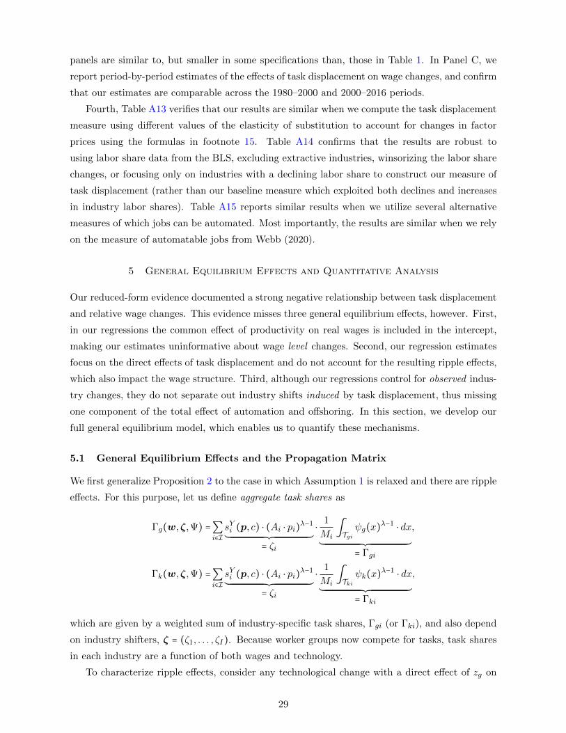
panels are similar to, but smaller in some specifications than, those in Table 1. In Panel C, we

report period-by-period estimates of the effects of task displacement on wage changes, and confirm

that our estimates are comparable across the 1980–2000 and 2000–2016 periods.

Fourth, Table A13 verifies that our results are similar when we compute the task displacement

measure using different values of the elasticity of substitution to account for changes in factor

prices using the formulas in footnote 15. Table A14 confirms that the results are robust to

using labor share data from the BLS, excluding extractive industries, winsorizing the labor share

changes, or focusing only on industries with a declining labor share to construct our measure of

task displacement (rather than our baseline measure which exploited both declines and increases

in industry labor shares). Table A15 reports similar results when we utilize several alternative

measures of which jobs can be automated. Most importantly, the results are similar when we rely

on the measure of automatable jobs from Webb (2020).

5 General Equilibrium Effects and Quantitative Analysis

Our reduced-form evidence documented a strong negative relationship between task displacement

and relative wage changes. This evidence misses three general equilibrium effects, however. First,

in our regressions the common effect of productivity on real wages is included in the intercept,

making our estimates uninformative about wage level changes. Second, our regression estimates

focus on the direct effects of task displacement and do not account for the resulting ripple effects,

which also impact the wage structure. Third, although our regressions control for observed indus-

try changes, they do not separate out industry shifts induced by task displacement, thus missing

one component of the total effect of automation and offshoring. In this section, we develop our

full general equilibrium model, which enables us to quantify these mechanisms.

5.1 General Equilibrium Effects and the Propagation Matrix

We first generalize Proposition 2 to the case in which Assumption 1 is relaxed and there are ripple

effects. For this purpose, let us define aggregate task shares as

Γg(w,ζ,Ψ) =∑i∈I

sYi (p, c) ⋅ (Ai ⋅ pi)λ−1

´¹¹¹¹¹¹¹¹¹¹¹¹¹¹¹¹¹¹¹¹¹¹¹¹¹¹¹¹¹¹¹¹¹¹¹¹¹¹¹¹¹¹¹¹¹¹¹¹¹¹¹¹¹¹¹¹¹¹¹¹¸¹¹¹¹¹¹¹¹¹¹¹¹¹¹¹¹¹¹¹¹¹¹¹¹¹¹¹¹¹¹¹¹¹¹¹¹¹¹¹¹¹¹¹¹¹¹¹¹¹¹¹¹¹¹¹¹¹¹¹¹¶= ζi

⋅1

Mi∫Tgi

ψg(x)λ−1

⋅ dx

´¹¹¹¹¹¹¹¹¹¹¹¹¹¹¹¹¹¹¹¹¹¹¹¹¹¹¹¹¹¹¹¹¹¹¹¹¹¹¹¹¹¹¹¹¹¹¹¹¹¹¹¹¹¹¹¹¹¹¹¹¹¹¹¸¹¹¹¹¹¹¹¹¹¹¹¹¹¹¹¹¹¹¹¹¹¹¹¹¹¹¹¹¹¹¹¹¹¹¹¹¹¹¹¹¹¹¹¹¹¹¹¹¹¹¹¹¹¹¹¹¹¹¹¹¹¹¹¹¶= Γgi

,

Γk(w,ζ,Ψ) =∑i∈I

sYi (p, c) ⋅ (Ai ⋅ pi)λ−1

´¹¹¹¹¹¹¹¹¹¹¹¹¹¹¹¹¹¹¹¹¹¹¹¹¹¹¹¹¹¹¹¹¹¹¹¹¹¹¹¹¹¹¹¹¹¹¹¹¹¹¹¹¹¹¹¹¹¹¹¹¸¹¹¹¹¹¹¹¹¹¹¹¹¹¹¹¹¹¹¹¹¹¹¹¹¹¹¹¹¹¹¹¹¹¹¹¹¹¹¹¹¹¹¹¹¹¹¹¹¹¹¹¹¹¹¹¹¹¹¹¹¶= ζi

⋅1

Mi∫Tki

ψk(x)λ−1

⋅ dx

´¹¹¹¹¹¹¹¹¹¹¹¹¹¹¹¹¹¹¹¹¹¹¹¹¹¹¹¹¹¹¹¹¹¹¹¹¹¹¹¹¹¹¹¹¹¹¹¹¹¹¹¹¹¹¹¹¹¹¹¹¹¹¹¹¸¹¹¹¹¹¹¹¹¹¹¹¹¹¹¹¹¹¹¹¹¹¹¹¹¹¹¹¹¹¹¹¹¹¹¹¹¹¹¹¹¹¹¹¹¹¹¹¹¹¹¹¹¹¹¹¹¹¹¹¹¹¹¹¹¶= Γki

,

which are given by a weighted sum of industry-specific task shares, Γgi (or Γki), and also depend

on industry shifters, ζ = (ζ1, . . . , ζI). Because worker groups now compete for tasks, task shares

in each industry are a function of both wages and technology.

To characterize ripple effects, consider any technological change with a direct effect of zg on

29

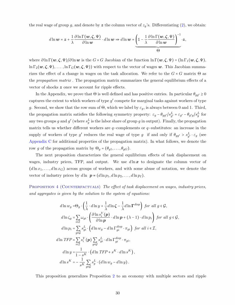
the real wage of group g, and denote by z the column vector of zg’s. Differentiating (2), we obtain:

d lnw = z +1

λ

∂ ln Γ(w,ζ,Ψ)

∂ lnw⋅ d lnw⇒ d lnw = (1 −

1

λ

∂ ln Γ(w,ζ,Ψ)

∂ lnw)

−1

´¹¹¹¹¹¹¹¹¹¹¹¹¹¹¹¹¹¹¹¹¹¹¹¹¹¹¹¹¹¹¹¹¹¹¹¹¹¹¹¹¹¹¹¹¹¹¹¹¹¹¹¹¹¹¹¹¹¹¹¹¹¹¹¹¹¹¹¹¹¹¹¹¹¹¹¹¹¹¸¹¹¹¹¹¹¹¹¹¹¹¹¹¹¹¹¹¹¹¹¹¹¹¹¹¹¹¹¹¹¹¹¹¹¹¹¹¹¹¹¹¹¹¹¹¹¹¹¹¹¹¹¹¹¹¹¹¹¹¹¹¹¹¹¹¹¹¹¹¹¹¹¹¹¹¹¹¹¹¶Θ

⋅z,

where ∂ ln Γ(w,ζ,Ψ)/∂ lnw is the G×G Jacobian of the function ln Γ(w,ζ,Ψ) = (ln Γ1(w,ζ,Ψ),

ln Γ2(w,ζ,Ψ), . . . , ln ΓG(w,ζ,Ψ)) with respect to the vector of wages w. This Jacobian summa-

rizes the effect of a change in wages on the task allocation. We refer to the G ×G matrix Θ as

the propagation matrix . The propagation matrix summarizes the general equilibrium effects of a

vector of shocks z once we account for ripple effects.

In the Appendix, we prove that Θ is well defined and has positive entries. In particular θgg′ ≥ 0

captures the extent to which workers of type g′ compete for marginal tasks against workers of type

g. Second, we show that the row sum of Θ, which we label by εg, is always between 0 and 1. Third,

the propagation matrix satisfies the following symmetry property: εg − θgg′/sLg′ = εg′ − θg′g/s

Lg for

any two groups g and g′ (where sLg is the labor share of group g in output). Finally, the propagation

matrix tells us whether different workers are q−complements or q−substitutes: an increase in the

supply of workers of type g′ reduces the real wage of type g if and only if θgg′ > sLg′ ⋅ εg (see

Appendix C for additional properties of the propagation matrix). In what follows, we denote the

row g of the propagation matrix by Θg = (θg1, . . . , θgG).

The next proposition characterizes the general equilibrium effects of task displacement on

wages, industry prices, TFP, and output. We use d lnx to designate the column vector of

(d lnx1, . . . , d lnxG) across groups of workers, and with some abuse of notation, we denote the

vector of industry prices by d ln p = (d lnp1, d lnp2, . . . , d lnpI).

Proposition 4 (Counterfactuals) The effect of task displacement on wages, industry prices,

and aggregates is given by the solution to the system of equations:

d lnwg =Θg ⋅ (1

λ⋅ d ln y +

1

λd lnζ −

1

λd lnΓdisp

) for all g ∈ G,

d ln ζg =∑i∈I

ωgi ⋅ (∂ ln sYi (p)

∂ lnp⋅ d lnp + (λ − 1) ⋅ d lnpi) for all g ∈ G,

d lnpi =∑g∈G

sLgi ⋅ (d lnwg − d ln Γdispgi ⋅ πgi) for all i ∈ I,

d ln TFP =∑i∈I

sYi (p)∑g∈G

sLgi ⋅ d ln Γdispgi ⋅ πgi,

d ln y =1

1 − sK⋅ (d ln TFP + sK ⋅ d ln sK) ,

d ln sK = −1

sK∑g∈G

sLg ⋅ (d lnwg − d ln y) .

This proposition generalizes Proposition 2 to an economy with multiple sectors and ripple

30

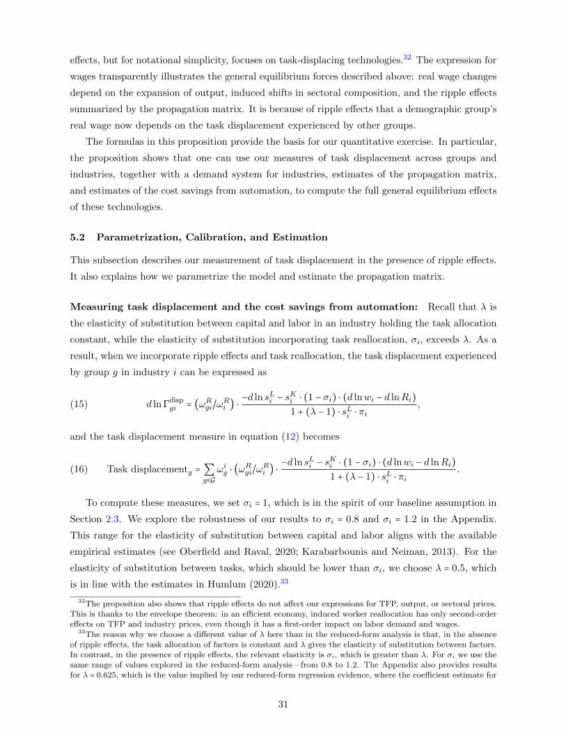
effects, but for notational simplicity, focuses on task-displacing technologies.32 The expression for

wages transparently illustrates the general equilibrium forces described above: real wage changes

depend on the expansion of output, induced shifts in sectoral composition, and the ripple effects

summarized by the propagation matrix. It is because of ripple effects that a demographic group’s

real wage now depends on the task displacement experienced by other groups.

The formulas in this proposition provide the basis for our quantitative exercise. In particular,

the proposition shows that one can use our measures of task displacement across groups and

industries, together with a demand system for industries, estimates of the propagation matrix,

and estimates of the cost savings from automation, to compute the full general equilibrium effects

of these technologies.

5.2 Parametrization, Calibration, and Estimation

This subsection describes our measurement of task displacement in the presence of ripple effects.

It also explains how we parametrize the model and estimate the propagation matrix.

Measuring task displacement and the cost savings from automation: Recall that λ is

the elasticity of substitution between capital and labor in an industry holding the task allocation

constant, while the elasticity of substitution incorporating task reallocation, σi, exceeds λ. As a

result, when we incorporate ripple effects and task reallocation, the task displacement experienced

by group g in industry i can be expressed as

d ln Γdispgi = (ωRgi/ω

Ri ) ⋅

−d ln sLi − sKi ⋅ (1 − σi) ⋅ (d lnwi − d lnRi)

1 + (λ − 1) ⋅ sLi ⋅ πi,(15)

and the task displacement measure in equation (12) becomes

Task displacementg = ∑g∈G

ωig ⋅ (ωRgi/ω

Ri ) ⋅

−d ln sLi − sKi ⋅ (1 − σi) ⋅ (d lnwi − d lnRi)

1 + (λ − 1) ⋅ sLi ⋅ πi.(16)

To compute these measures, we set σi = 1, which is in the spirit of our baseline assumption in

Section 2.3. We explore the robustness of our results to σi = 0.8 and σi = 1.2 in the Appendix.

This range for the elasticity of substitution between capital and labor aligns with the available

empirical estimates (see Oberfield and Raval, 2020; Karabarbounis and Neiman, 2013). For the

elasticity of substitution between tasks, which should be lower than σi, we choose λ = 0.5, which

is in line with the estimates in Humlum (2020).33

32The proposition also shows that ripple effects do not affect our expressions for TFP, output, or sectoral prices.This is thanks to the envelope theorem: in an efficient economy, induced worker reallocation has only second-ordereffects on TFP and industry prices, even though it has a first-order impact on labor demand and wages.

33The reason why we choose a different value of λ here than in the reduced-form analysis is that, in the absenceof ripple effects, the task allocation of factors is constant and λ gives the elasticity of substitution between factors.In contrast, in the presence of ripple effects, the relevant elasticity is σi, which is greater than λ. For σi we use thesame range of values explored in the reduced-form analysis—from 0.8 to 1.2. The Appendix also provides resultsfor λ = 0.625, which is the value implied by our reduced-form regression evidence, where the coefficient estimate for

31

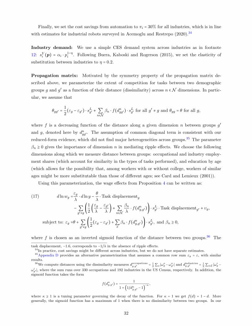
Finally, we set the cost savings from automation to πi = 30% for all industries, which is in line

with estimates for industrial robots surveyed in Acemoglu and Restrepo (2020).34

Industry demand: We use a simple CES demand system across industries as in footnote

12: sYi (p) = αi ⋅ p1−ηi . Following Buera, Kaboski and Rogerson (2015), we set the elasticity of

substitution between industries to η = 0.2.

Propagation matrix: Motivated by the symmetry property of the propagation matrix de-

scribed above, we parameterize the extent of competition for tasks between two demographic

groups g and g′ as a function of their distance (dissimilarity) across n ∈ N dimensions. In partic-

ular, we assume that

θgg′ =1

2(εg − εg′) ⋅ s

Lg′ + ∑

n∈N

βn ⋅ f(dngg′) ⋅ s

Lg′ for all g′ ≠ g and θgg = θ for all g,

where f is a decreasing function of the distance along a given dimension n between groups g′

and g, denoted here by dngg′ . The assumption of common diagonal term is consistent with our

reduced-form evidence, which did not find major heterogeneities across groups.35 The parameter

βn ≥ 0 gives the importance of dimension n in mediating ripple effects. We choose the following

dimensions along which we measure distance between groups: occupational and industry employ-

ment shares (which account for similarity in the types of tasks performed), and education by age

(which allows for the possibility that, among workers with or without college, workers of similar

ages might be more substitutable than those of different ages; see Card and Lemieux (2001)).

Using this parameterization, the wage effects from Proposition 4 can be written as:

d lnwg =εg

λ⋅ d ln y −

θ

λ⋅Task displacementg(17)

− ∑g′≠g

(1

2(εg

λ−εg′

λ) + ∑

n∈N

βnλ⋅ f(dng,g′)) ⋅ s

Lg′ ⋅Task displacementg′ + υg,

subject to: εg =θ + ∑g′≠g

(1

2(εg − εg′) +∑

x

βn ⋅ f(dng,g′)) ⋅ s

Lg′ , and βn ≥ 0,

where f is chosen as an inverted sigmoid function of the distance between two groups.36 The

task displacement, −1.6, corresponds to −1/λ in the absence of ripple effects.34In practice, cost savings might be different across industries, but we do not have separate estimates.35Appendix D provides an alternative parametrization that assumes a common row sum εg = ε, with similar

results.36We compute distances using the dissimilarity measures doccupations

g,g′= 1

2 ∑o ∣ωog −ωog′ ∣ and dindustriesg,g′ = 1

2 ∑i∈I ∣ωig −ωig′ ∣, where the sum runs over 330 occupations and 192 industries in the US Census, respectively. In addition, thesigmoid function takes the form

f(dng,g′) =1

1 + (1/dng,g′− 1)

−κ ,

where κ ≥ 1 is a tuning parameter governing the decay of the function. For κ = 1 we get f(d) = 1 − d. Moregenerally, the sigmoid function has a maximum of 1 when there is no dissimilarity between two groups. In our

32

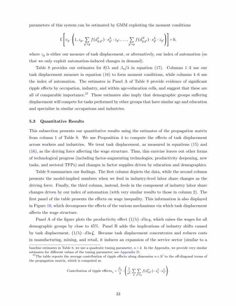
parameters of this system can be estimated by GMM exploiting the moment conditions

E⎡⎢⎢⎢⎢⎣

υg ⋅⎛

⎝1, zg, ∑

g′≠g

f(d1g,g′) ⋅ s

Lg′ ⋅ zg′ , . . . , ∑

g′≠g

f(dNg,g′) ⋅ sLg′ ⋅ zg′

⎞

⎠

⎤⎥⎥⎥⎥⎦

= 0,

where zg is either our measure of task displacement, or alternatively, our index of automation (so

that we only exploit automation-induced changes in demand).

Table 8 provides our estimates for θ/λ and βn/λ in equation (17). Columns 1–3 use our

task displacement measure in equation (16) to form moment conditions, while columns 4–6 use

the index of automation. The estimates in Panel A of Table 8 provide evidence of significant

ripple effects by occupation, industry, and within age×education cells, and suggest that these are

all of comparable importance.37 These estimates also imply that demographic groups suffering

displacement will compete for tasks performed by other groups that have similar age and education

and specialize in similar occupations and industries.

5.3 Quantitative Results

This subsection presents our quantitative results using the estimates of the propagation matrix

from column 1 of Table 8. We use Proposition 4 to compute the effects of task displacement

across workers and industries. We treat task displacement, as measured in equations (15) and

(16), as the driving force affecting the wage structure. Thus, this exercise leaves out other forms

of technological progress (including factor-augmenting technologies, productivity deepening, new

tasks, and sectoral TFPs) and changes in factor supplies driven by education and demographics.

Table 9 summarizes our findings. The first column depicts the data, while the second column

presents the model-implied numbers when we feed in industry-level labor share changes as the

driving force. Finally, the third column, instead, feeds in the component of industry labor share

changes driven by our index of automation (with very similar results to those in column 2). The

first panel of the table presents the effects on wage inequality. This information is also displayed

in Figure 10, which decomposes the effects of the various mechanisms via which task displacement

affects the wage structure.

Panel A of the figure plots the productivity effect (1/λ) ⋅ d ln y, which raises the wages for all

demographic groups by close to 45%. Panel B adds the implications of industry shifts caused

by task displacement, (1/λ) ⋅ d lnζ. Because task displacement concentrates and reduces costs

in manufacturing, mining, and retail, it induces an expansion of the service sector (similar to a

baseline estimates in Table 8, we use a quadratic tuning parameter, κ = 2. In the Appendix, we provide very similarestimates for different values of the tuning parameter; see Appendix D.

37The table reports the average contribution of ripple effects along dimension n ∈ N to the off-diagonal terms ofthe propagation matrix, which is computed as

Contribution of ripple effectsn =βnλ⋅⎛⎝

1

sL∑g

∑g′≠g

f(dngg′) ⋅ sLg ⋅ sLg′⎞⎠.

33

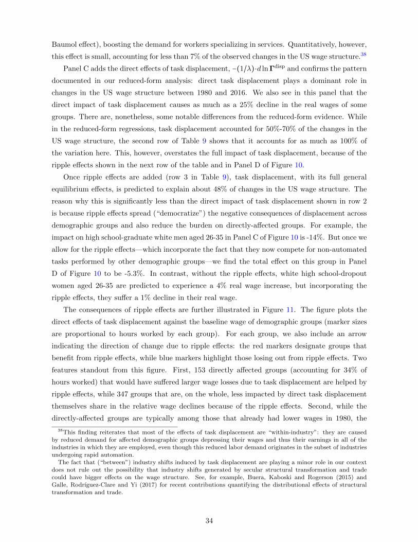
Baumol effect), boosting the demand for workers specializing in services. Quantitatively, however,

this effect is small, accounting for less than 7% of the observed changes in the US wage structure.38

Panel C adds the direct effects of task displacement, −(1/λ)⋅d lnΓdisp and confirms the pattern

documented in our reduced-form analysis: direct task displacement plays a dominant role in

changes in the US wage structure between 1980 and 2016. We also see in this panel that the

direct impact of task displacement causes as much as a 25% decline in the real wages of some

groups. There are, nonetheless, some notable differences from the reduced-form evidence. While

in the reduced-form regressions, task displacement accounted for 50%-70% of the changes in the

US wage structure, the second row of Table 9 shows that it accounts for as much as 100% of

the variation here. This, however, overstates the full impact of task displacement, because of the

ripple effects shown in the next row of the table and in Panel D of Figure 10.

Once ripple effects are added (row 3 in Table 9), task displacement, with its full general

equilibrium effects, is predicted to explain about 48% of changes in the US wage structure. The

reason why this is significantly less than the direct impact of task displacement shown in row 2

is because ripple effects spread (“democratize”) the negative consequences of displacement across

demographic groups and also reduce the burden on directly-affected groups. For example, the

impact on high school-graduate white men aged 26-35 in Panel C of Figure 10 is -14%. But once we

allow for the ripple effects—which incorporate the fact that they now compete for non-automated

tasks performed by other demographic groups—we find the total effect on this group in Panel

D of Figure 10 to be -5.3%. In contrast, without the ripple effects, white high school-dropout

women aged 26-35 are predicted to experience a 4% real wage increase, but incorporating the

ripple effects, they suffer a 1% decline in their real wage.

The consequences of ripple effects are further illustrated in Figure 11. The figure plots the

direct effects of task displacement against the baseline wage of demographic groups (marker sizes

are proportional to hours worked by each group). For each group, we also include an arrow

indicating the direction of change due to ripple effects: the red markers designate groups that

benefit from ripple effects, while blue markers highlight those losing out from ripple effects. Two

features standout from this figure. First, 153 directly affected groups (accounting for 34% of

hours worked) that would have suffered larger wage losses due to task displacement are helped by

ripple effects, while 347 groups that are, on the whole, less impacted by direct task displacement

themselves share in the relative wage declines because of the ripple effects. Second, while the

directly-affected groups are typically among those that already had lower wages in 1980, the

38This finding reiterates that most of the effects of task displacement are “within-industry”: they are causedby reduced demand for affected demographic groups depressing their wages and thus their earnings in all of theindustries in which they are employed, even though this reduced labor demand originates in the subset of industriesundergoing rapid automation.

The fact that (“between”) industry shifts induced by task displacement are playing a minor role in our contextdoes not rule out the possibility that industry shifts generated by secular structural transformation and tradecould have bigger effects on the wage structure. See, for example, Buera, Kaboski and Rogerson (2015) andGalle, Rodrıguez-Clare and Yi (2017) for recent contributions quantifying the distributional effects of structuraltransformation and trade.

34

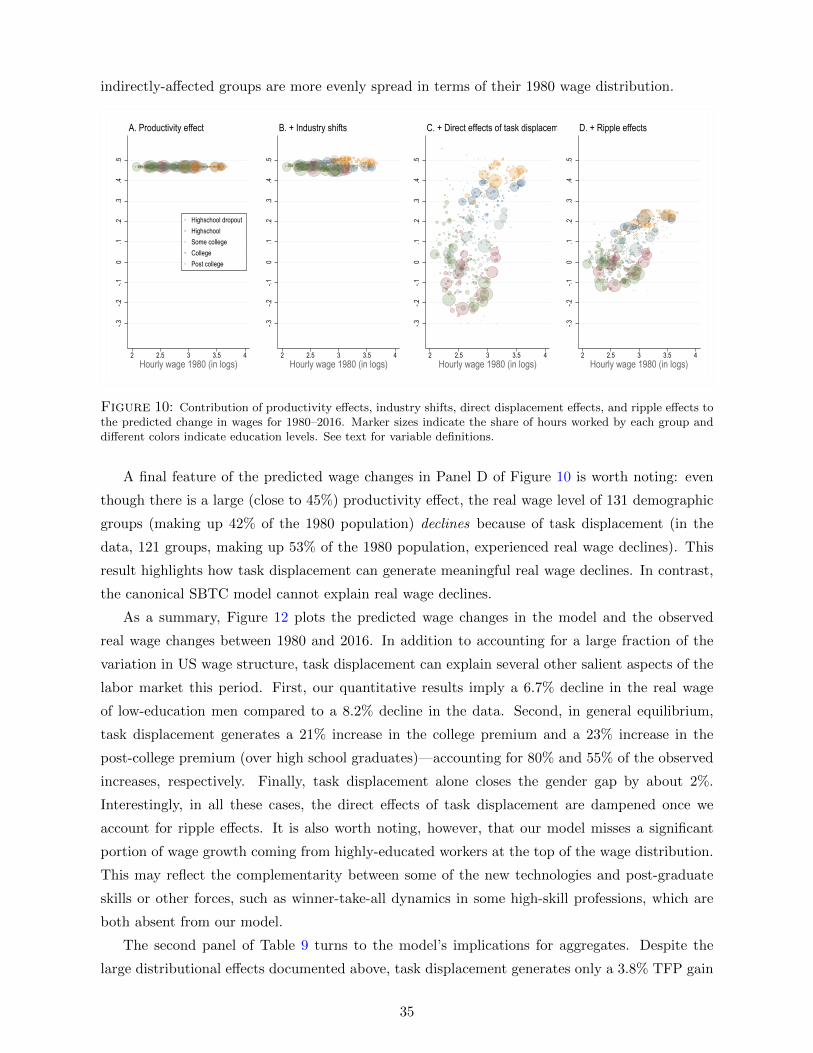
indirectly-affected groups are more evenly spread in terms of their 1980 wage distribution.

-.3-.2

-.10

.1.2

.3.4

.5

2 2.5 3 3.5 4Hourly wage 1980 (in logs)

Highschool dropoutHighschoolSome collegeCollegePost college

A. Productivity effect

-.3-.2

-.10

.1.2

.3.4

.5

2 2.5 3 3.5 4Hourly wage 1980 (in logs)

B. + Industry shifts

-.3-.2

-.10

.1.2

.3.4

.5

2 2.5 3 3.5 4Hourly wage 1980 (in logs)

C. + Direct effects of task displacement

-.3-.2

-.10

.1.2

.3.4

.5

2 2.5 3 3.5 4Hourly wage 1980 (in logs)

D. + Ripple effects

Figure 10: Contribution of productivity effects, industry shifts, direct displacement effects, and ripple effects tothe predicted change in wages for 1980–2016. Marker sizes indicate the share of hours worked by each group anddifferent colors indicate education levels. See text for variable definitions.

A final feature of the predicted wage changes in Panel D of Figure 10 is worth noting: even

though there is a large (close to 45%) productivity effect, the real wage level of 131 demographic

groups (making up 42% of the 1980 population) declines because of task displacement (in the

data, 121 groups, making up 53% of the 1980 population, experienced real wage declines). This

result highlights how task displacement can generate meaningful real wage declines. In contrast,

the canonical SBTC model cannot explain real wage declines.

As a summary, Figure 12 plots the predicted wage changes in the model and the observed

real wage changes between 1980 and 2016. In addition to accounting for a large fraction of the

variation in US wage structure, task displacement can explain several other salient aspects of the

labor market this period. First, our quantitative results imply a 6.7% decline in the real wage

of low-education men compared to a 8.2% decline in the data. Second, in general equilibrium,

task displacement generates a 21% increase in the college premium and a 23% increase in the

post-college premium (over high school graduates)—accounting for 80% and 55% of the observed

increases, respectively. Finally, task displacement alone closes the gender gap by about 2%.

Interestingly, in all these cases, the direct effects of task displacement are dampened once we

account for ripple effects. It is also worth noting, however, that our model misses a significant

portion of wage growth coming from highly-educated workers at the top of the wage distribution.

This may reflect the complementarity between some of the new technologies and post-graduate

skills or other forces, such as winner-take-all dynamics in some high-skill professions, which are

both absent from our model.

The second panel of Table 9 turns to the model’s implications for aggregates. Despite the

large distributional effects documented above, task displacement generates only a 3.8% TFP gain

35

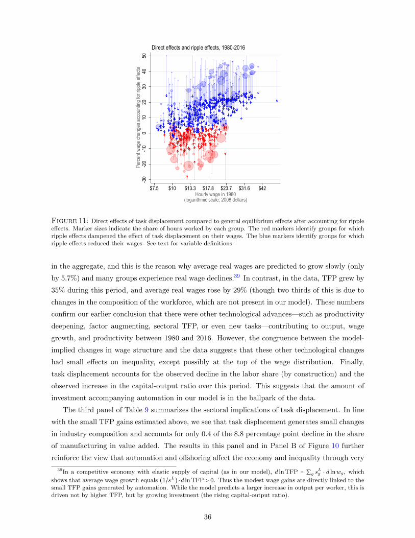
-30

-20

-10

010

2030

4050

Perce

nt wa

ge ch

ange

s acc

ounti

ng fo

r ripp

le eff

ects

$7.5 $10 $13.3 $17.8 $23.7 $31.6 $42Hourly wage in 1980

(logarithmic scale, 2008 dollars)

Direct effects and ripple effects, 1980-2016

Figure 11: Direct effects of task displacement compared to general equilibrium effects after accounting for rippleeffects. Marker sizes indicate the share of hours worked by each group. The red markers identify groups for whichripple effects dampened the effect of task displacement on their wages. The blue markers identify groups for whichripple effects reduced their wages. See text for variable definitions.

in the aggregate, and this is the reason why average real wages are predicted to grow slowly (only

by 5.7%) and many groups experience real wage declines.39 In contrast, in the data, TFP grew by

35% during this period, and average real wages rose by 29% (though two thirds of this is due to

changes in the composition of the workforce, which are not present in our model). These numbers

confirm our earlier conclusion that there were other technological advances—such as productivity

deepening, factor augmenting, sectoral TFP, or even new tasks—contributing to output, wage

growth, and productivity between 1980 and 2016. However, the congruence between the model-

implied changes in wage structure and the data suggests that these other technological changes

had small effects on inequality, except possibly at the top of the wage distribution. Finally,

task displacement accounts for the observed decline in the labor share (by construction) and the

observed increase in the capital-output ratio over this period. This suggests that the amount of

investment accompanying automation in our model is in the ballpark of the data.

The third panel of Table 9 summarizes the sectoral implications of task displacement. In line

with the small TFP gains estimated above, we see that task displacement generates small changes

in industry composition and accounts for only 0.4 of the 8.8 percentage point decline in the share

of manufacturing in value added. The results in this panel and in Panel B of Figure 10 further

reinforce the view that automation and offshoring affect the economy and inequality through very

39In a competitive economy with elastic supply of capital (as in our model), d ln TFP = ∑g sLg ⋅ d lnwg, which

shows that average wage growth equals (1/sL) ⋅d ln TFP > 0. Thus the modest wage gains are directly linked to thesmall TFP gains generated by automation. While the model predicts a larger increase in output per worker, this isdriven not by higher TFP, but by growing investment (the rising capital-output ratio).

36

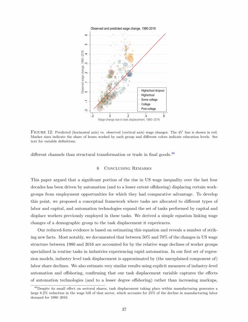
-.2-.1

0.1

.2.3

.4.5

.6Ob

serve

d wag

e cha

nge,

1980

--201

6

-.2 0 .2 .4 .6Wage change due to task displacement, 1980--2016

Highschool dropoutHighschoolSome collegeCollegePost college

Observed and predicted wage change, 1980-2016

Figure 12: Predicted (horizontal axis) vs. observed (vertical axis) wage changes. The 45○ line is shown in red.Marker sizes indicate the share of hours worked by each group and different colors indicate education levels. Seetext for variable definitions.

different channels than structural transformation or trade in final goods.40

6 Concluding Remarks

This paper argued that a significant portion of the rise in US wage inequality over the last four

decades has been driven by automation (and to a lesser extent offshoring) displacing certain work-

groups from employment opportunities for which they had comparative advantage. To develop

this point, we proposed a conceptual framework where tasks are allocated to different types of

labor and capital, and automation technologies expand the set of tasks performed by capital and

displace workers previously employed in these tasks. We derived a simple equation linking wage

changes of a demographic group to the task displacement it experiences.

Our reduced-form evidence is based on estimating this equation and reveals a number of strik-

ing new facts. Most notably, we documented that between 50% and 70% of the changes in US wage

structure between 1980 and 2016 are accounted for by the relative wage declines of worker groups

specialized in routine tasks in industries experiencing rapid automation. In our first set of regres-

sion models, industry level task displacement is approximated by (the unexplained component of)

labor share declines. We also estimate very similar results using explicit measures of industry-level

automation and offshoring, confirming that our task displacement variable captures the effects

of automation technologies (and to a lesser degree offshoring) rather than increasing markups,

40Despite its small effect on sectoral shares, task displacement taking place within manufacturing generates alarge 8.2% reduction in the wage bill of that sector, which accounts for 25% of the decline in manufacturing labordemand for 1980–2016.

37

industry concentration, or import competition. These alternative economic trends themselves do

not appear to play a major role in the evolution of the US wage structure.

Our reduced-form regressions estimate the direct effects of task displacement on relative wages,

but miss important general equilibrium forces. We developed a methodology to quantify the gen-

eral equilibrium effects of task displacement, which can account for the implications of automation

working through productivity gains, ripple effects and changes in industry composition. Our full

quantitative evaluation shows that task displacement explains close to 50% of the observed changes

in US wage structure. Most notably, task displacement leads to sizable increases in wage inequal-

ity, but only small productivity gains—thus providing a possible resolution to a puzzling feature

of US data.

There are several interesting areas for future research. First, our framework has been static,

and thus any effects from capital accumulation, dynamic incentives for the development of new

technologies and education and skill acquisition are absent. Incorporating those is an important

direction for future research. Second, and relatedly, we did not attempt to model and estimate

the effects of technologies introducing new labor-intensive tasks (which we argued to have been

important in previous work, Acemoglu and Restrepo, 2018). This is yet another avenue for future

research. Finally, our empirical work has been confined to the US and the 1980-2016 period,

for which we have all the data components necessary for implementing our reduced-form and

structural estimation. Expanding these data sources and the empirical exploration of the role of

task displacement to earlier periods and other economies is an important direction for research that

may help us understand the technological and institutional reasons why the US wage structure

was quite stable for the three decades leading up to the mid-1970s.

References

Acemoglu, D., and D. Autor (2011): Skills, Tasks and Technologies: Implications for Employment

and Earningsvol. 4 of Handbook of Labor Economics, chap. 12, pp. 1043–1171. Elsevier.

Acemoglu, D., D. Autor, D. Dorn, G. H. Hanson, and B. Price (2016): “Import Competition

and the Great US Employment Sag of the 2000s,” Journal of Labor Economics, 34(S1), S141–S198.

Acemoglu, D., D. Autor, J. Hazell, and P. Restrepo (2020): “AI and Jobs: Evidence from Online

Vacancies,” Working Paper 28257, National Bureau of Economic Research.

Acemoglu, D., C. Lelarge, and P. Restrepo (2020): “Competing with Robots: Firm-Level Evidence

from France,” in AEA Papers and Proceedings, vol. 110, pp. 383–88.

Acemoglu, D., and P. Restrepo (2018): “The Race between Man and Machine: Implications of

Technology for Growth, Factor Shares, and Employment,” American Economic Review, 108(6), 1488–

1542.

(2019): “Automation and New Tasks: How Technology Displaces and Reinstates Labor,” Journal

of Economic Perspectives, 33(2), 3–30.

(2020): “Robots and Jobs: Evidence from US Labor Markets,” Journal of Political Economy,

128(6), 2188–2244.

Acemoglu, D., and F. Zilibotti (2001): “Productivity Differences*,” The Quarterly Journal of Eco-

nomics, 116(2), 563–606.

38

Atalay, E., P. Phongthiengtham, S. Sotelo, and D. Tannenbaum (2020): “The Evolution of

Work in the United States,” American Economic Journal: Applied Economics, 12(2), 1–34.

Autor, D., and D. Dorn (2013): “The Growth of Low-skill Service Jobs and the Polarization of the US

Labor Market,” American Economic Review, 103(5), 1553–97.

Autor, D., D. Dorn, L. F. Katz, C. Patterson, and J. Van Reenen (2020): “The Fall of the

Labor Share and the Rise of Superstar Firms,” The Quarterly Journal of Economics, 135(2), 645–709.

Autor, D. H. (2019): “Work of the Past, Work of the Future,” AEA Papers and Proceedings, 109, 1–32.

Autor, D. H., L. F. Katz, and A. B. Krueger (1998): “Computing Inequality: Have Computers

Changed the Labor Market?,” The Quarterly Journal of Economics, 113(4), 1169–1213.

Autor, D. H., F. Levy, and R. J. Murnane (2003): “The Skill Content of Recent Technological

Change: An Empirical Exploration,” The Quarterly Journal of Economics, 118(4), 1279–1333.

Berman, E., J. Bound, and Z. Griliches (1994): “Changes in the Demand for Skilled Labor within

U. S. Manufacturing: Evidence from the Annual Survey of Manufactures,” The Quarterly Journal of

Economics, 109(2), 367–397.

Berman, E., J. Bound, and S. Machin (1998): “Implications of Skill-Biased Technological Change:

International Evidence,” The Quarterly Journal of Economics, 113(4), 1245–1279.

Bound, J., and G. Johnson (1992): “Changes in the Structure of Wages in the 1980’s: An Evaluation

of Alternative Explanations,” American Economic Review, 82(3), 371–92.

Buera, F. J., J. P. Kaboski, and R. Rogerson (2015): “Skill Biased Structural Change,” Discussion

paper, National Bureau of Economic Research.

Burstein, A., E. Morales, and J. Vogel (2019): “Changes in Between-group Inequality: Computers,

Occupations, and International Trade,” American Economic Journal: Macroeconomics, 11(2), 348–400.

Card, D., and T. Lemieux (2001): “Can Falling Supply Explain the Rising Return to College for

Younger Men? A Cohort-Based Analysis*,” The Quarterly Journal of Economics, 116(2), 705–746.

Dao, M. C., M. Das, and Z. Koczan (2019): “Why is Labour Receiving a Smaller Share of Global

Income?,” Economic Policy, 34(100), 723–759.

David, H., D. Dorn, and G. H. Hanson (2013): “The China Syndrome: Local Labor Market Effects

of Import Competition in the United States,” American Economic Review, 103(6), 2121–68.

De Loecker, J., J. Eeckhout, and G. Unger (2020): “The Rise of Market Power and the Macroeco-

nomic Implications,” The Quarterly Journal of Economics, 135(2), 561–644.

DiNardo, J., N. M. Fortin, and T. Lemieux (1996): “Labor Market Institutions and the Distribution

of Wages, 1973-1992: A Semiparametric Approach,” Econometrica: Journal of the Econometric Society,

pp. 1001–1044.

Elsby, M. W., B. Hobijn, and A. Sahin (2013): “The Decline of the US Labor Share,” Brookings

Papers on Economic Activity, 2013(2), 1–63.

Feenstra, R. C., and G. H. Hanson (1999): “The Impact of Outsourcing and High-technology Capital

on Wages: Estimates for the United States, 1979–1990,” The Quarterly Journal of Economics, 114(3),

907–940.

Fernald, J. (2014): “A Quarterly, Utilization-adjusted Series on Total Factor Productivity,” Discussion

paper, Federal Reserve Bank of San Francisco.

Galle, S., A. Rodrıguez-Clare, and M. Yi (2017): “Slicing the Pie: Quantifying the Aggregate and

Distributional Effects of Trade,” Working Paper 23737, National Bureau of Economic Research.

Goldin, C. D., and L. F. Katz (2008): The Race Between Education and Technology. Harvard University

Press Cambridge.

Goos, M., and A. Manning (2007): “Lousy and Lovely Jobs: The Rising Polarization of Work in

Britain,” The Review of Economics and Statistics, 89(1), 118–133.

39

Goos, M., A. Manning, and A. Salomons (2014): “Explaining Job Polarization: Routine-Biased

Technological Change and Offshoring,” American Economic Review, 104(8), 2509–26.

Gregory, T., A. Salomons, and U. Zierahn (2018): “Racing With or Against the Machine? Evidence

from Europe,” Working Paper No. 7247, CESifo Working Paper.

Griliches, Z. (1969): “Capital-Skill Complementarity,” The Review of Economics and Statistics, 51(4),

465–468.

Grossman, G. M., and E. Rossi-Hansberg (2008): “Trading Tasks: A Simple Theory of Offshoring,”

American Economic Review, 98(5), 1978–97.

Hubmer, J. (2020): “The Race Between Preferences and Technology,” Unpublished manuscript, University

of Pennsylvania.

Hubmer, J., and P. Restrepo (2021): “Not a Typical Firm: The Joint Dynamics of Firms, Labor Shares,

and Capital-Labor Substitution,” Working Paper 28579, National Bureau of Economic Research.

Humlum, A. (2020): “Robot Adoption and Labor Market Dynamics,” Working paper, University of

Chicago.

Jaimovich, N., I. Saporta-Eksten, H. E. Siu, and Y. Yedid-Levi (2020): “The Macroeconomics

of Automation: Data, Theory, and Policy Analysis,” Discussion paper, National Bureau of Economic

Research.

Karabarbounis, L., and B. Neiman (2013): “The Global Decline of the Labor Share,” The Quarterly

Journal of Economics, 129(1), 61–103.

(2018): “Accounting for Factorless Income,” NBER Working Papers 24404, National Bureau of

Economic Research, Inc.

Katz, L. F., and K. M. Murphy (1992): “Changes in Relative Wages, 1963–1987: Supply and Demand

factors,” The Quarterly Journal of Economics, 107(1), 35–78.

Kim, R., and J. Vogel (2021): “Trade Shocks and Labor Market Adjustment,” American Economic

Review: Insights, 3(1), 115–30.

Klenow, P. J., and A. Rodrıguez-Clare (1997): “The Neoclassical Revival in Growth Economics:

Has It Gone Too Far?,” NBER Macroeconomics Annual, 12, 73–103.

Krueger, A. B. (1993): “How Computers Have Changed the Wage Structure: Evidence from Microdata,

1984-1989,” The Quarterly Journal of Economics, 108(1), 33–60.

Krusell, P., L. E. Ohanian, J.-V. RAos-Rull, and G. L. Violante (2000): “Capital-Skill Com-

plementarity and Inequality: A Macroeconomic Analysis,” Econometrica, 68(5), 1029–1053.

Lee, S. Y. T., and Y. Shin (2017): “Horizontal and Vertical Polarization: Task-Specific Technological

Change in a Multi-Sector Economy,” Working Paper 23283, National Bureau of Economic Research.

Oberfield, E., and D. Raval (2020): “Micro Data and Macro Technology,” Econometrica.

Piketty, T. (2014): Capital in the Twenty-First Century. Harvard University Press, Cambridge.

Webb, M. (2020): “The Impact of Artificial Intelligence on the Labor Market,” Working paper, Stanford

University.

Wright, G. C. (2014): “Revisiting the Employment Impact of Offshoring,” European Economic Review,

66, 63–83.

Zeira, J. (1998): “Workers, Machines, and Economic Growth,” The Quarterly Journal of Economics,

113(4), 1091–1117.

40

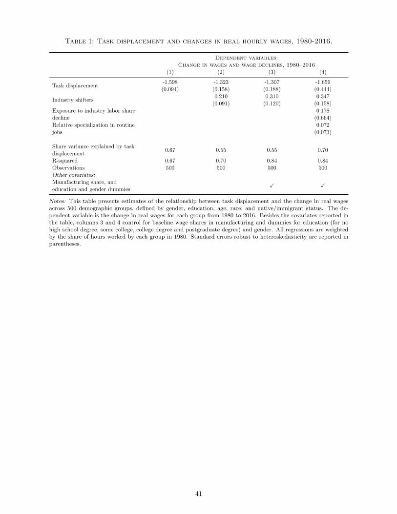
Table 1: Task displacement and changes in real hourly wages, 1980-2016.

Dependent variables:Change in wages and wage declines, 1980–2016

(1) (2) (3) (4)

Task displacement-1.598 -1.323 -1.307 -1.659(0.094) (0.158) (0.188) (0.444)

Industry shifters0.210 0.310 0.347

(0.091) (0.120) (0.158)Exposure to industry labor sharedecline

0.178(0.664)

Relative specialization in routinejobs

0.072(0.073)

Share variance explained by taskdisplacement

0.67 0.55 0.55 0.70

R-squared 0.67 0.70 0.84 0.84Observations 500 500 500 500Other covariates:Manufacturing share, andeducation and gender dummies

✓ ✓

Notes: This table presents estimates of the relationship between task displacement and the change in real wagesacross 500 demographic groups, defined by gender, education, age, race, and native/immigrant status. The de-pendent variable is the change in real wages for each group from 1980 to 2016. Besides the covariates reported inthe table, columns 3 and 4 control for baseline wage shares in manufacturing and dummies for education (for nohigh school degree, some college, college degree and postgraduate degree) and gender. All regressions are weightedby the share of hours worked by each group in 1980. Standard errors robust to heteroskedasticity are reported inparentheses.

41

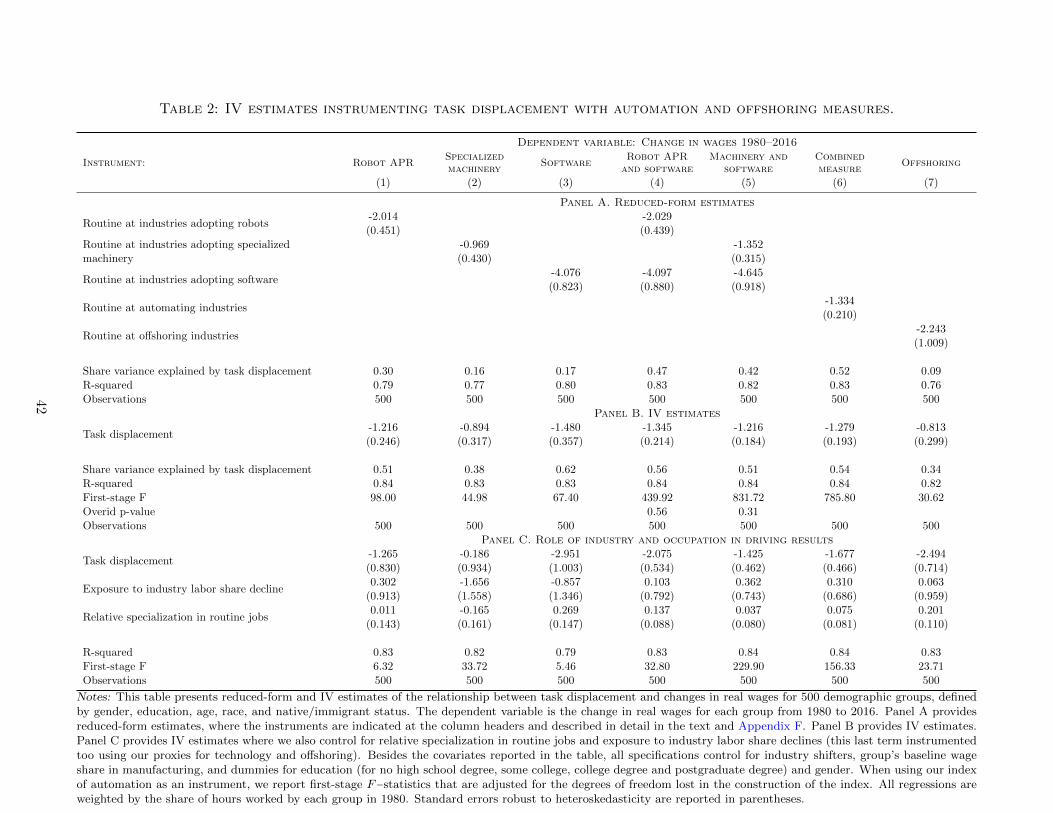
Table 2: IV estimates instrumenting task displacement with automation and offshoring measures.

Dependent variable: Change in wages 1980–2016

Instrument: Robot APRSpecializedmachinery

SoftwareRobot APR

and softwareMachinery and

softwareCombinedmeasure

Offshoring

(1) (2) (3) (4) (5) (6) (7)

Panel A. Reduced-form estimates

Routine at industries adopting robots-2.014 -2.029(0.451) (0.439)

Routine at industries adopting specializedmachinery

-0.969 -1.352(0.430) (0.315)

Routine at industries adopting software-4.076 -4.097 -4.645(0.823) (0.880) (0.918)

Routine at automating industries-1.334(0.210)

Routine at offshoring industries-2.243(1.009)

Share variance explained by task displacement 0.30 0.16 0.17 0.47 0.42 0.52 0.09R-squared 0.79 0.77 0.80 0.83 0.82 0.83 0.76Observations 500 500 500 500 500 500 500

Panel B. IV estimates

Task displacement-1.216 -0.894 -1.480 -1.345 -1.216 -1.279 -0.813(0.246) (0.317) (0.357) (0.214) (0.184) (0.193) (0.299)

Share variance explained by task displacement 0.51 0.38 0.62 0.56 0.51 0.54 0.34R-squared 0.84 0.83 0.83 0.84 0.84 0.84 0.82First-stage F 98.00 44.98 67.40 439.92 831.72 785.80 30.62Overid p-value 0.56 0.31Observations 500 500 500 500 500 500 500

Panel C. Role of industry and occupation in driving results

Task displacement-1.265 -0.186 -2.951 -2.075 -1.425 -1.677 -2.494(0.830) (0.934) (1.003) (0.534) (0.462) (0.466) (0.714)

Exposure to industry labor share decline0.302 -1.656 -0.857 0.103 0.362 0.310 0.063

(0.913) (1.558) (1.346) (0.792) (0.743) (0.686) (0.959)

Relative specialization in routine jobs0.011 -0.165 0.269 0.137 0.037 0.075 0.201

(0.143) (0.161) (0.147) (0.088) (0.080) (0.081) (0.110)

R-squared 0.83 0.82 0.79 0.83 0.84 0.84 0.83First-stage F 6.32 33.72 5.46 32.80 229.90 156.33 23.71Observations 500 500 500 500 500 500 500

Notes: This table presents reduced-form and IV estimates of the relationship between task displacement and changes in real wages for 500 demographic groups, definedby gender, education, age, race, and native/immigrant status. The dependent variable is the change in real wages for each group from 1980 to 2016. Panel A providesreduced-form estimates, where the instruments are indicated at the column headers and described in detail in the text and Appendix F. Panel B provides IV estimates.Panel C provides IV estimates where we also control for relative specialization in routine jobs and exposure to industry labor share declines (this last term instrumentedtoo using our proxies for technology and offshoring). Besides the covariates reported in the table, all specifications control for industry shifters, group’s baseline wageshare in manufacturing, and dummies for education (for no high school degree, some college, college degree and postgraduate degree) and gender. When using our indexof automation as an instrument, we report first-stage F−statistics that are adjusted for the degrees of freedom lost in the construction of the index. All regressions areweighted by the share of hours worked by each group in 1980. Standard errors robust to heteroskedasticity are reported in parentheses.

42

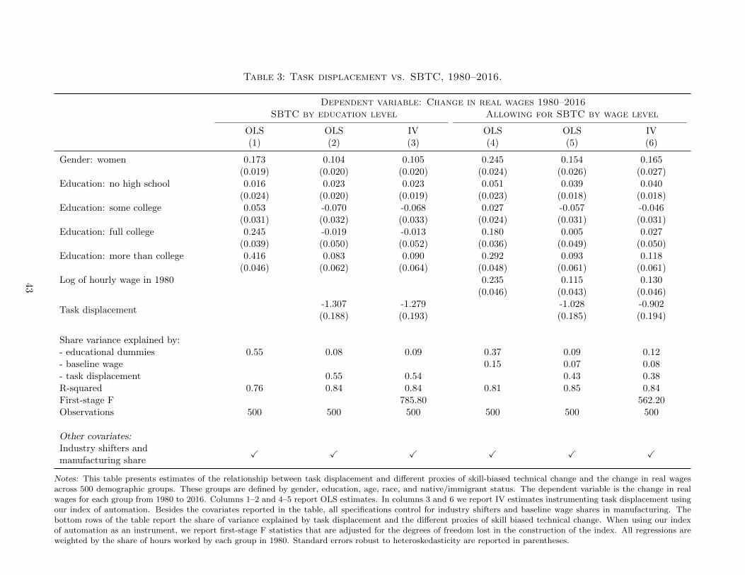
Table 3: Task displacement vs. SBTC, 1980–2016.

Dependent variable: Change in real wages 1980–2016SBTC by education level Allowing for SBTC by wage level

OLS OLS IV OLS OLS IV(1) (2) (3) (4) (5) (6)

Gender: women 0.173 0.104 0.105 0.245 0.154 0.165(0.019) (0.020) (0.020) (0.024) (0.026) (0.027)

Education: no high school 0.016 0.023 0.023 0.051 0.039 0.040(0.024) (0.020) (0.019) (0.023) (0.018) (0.018)

Education: some college 0.053 -0.070 -0.068 0.027 -0.057 -0.046(0.031) (0.032) (0.033) (0.024) (0.031) (0.031)

Education: full college 0.245 -0.019 -0.013 0.180 0.005 0.027(0.039) (0.050) (0.052) (0.036) (0.049) (0.050)

Education: more than college 0.416 0.083 0.090 0.292 0.093 0.118(0.046) (0.062) (0.064) (0.048) (0.061) (0.061)

Log of hourly wage in 1980 0.235 0.115 0.130(0.046) (0.043) (0.046)

Task displacement-1.307 -1.279 -1.028 -0.902(0.188) (0.193) (0.185) (0.194)

Share variance explained by:- educational dummies 0.55 0.08 0.09 0.37 0.09 0.12- baseline wage 0.15 0.07 0.08- task displacement 0.55 0.54 0.43 0.38R-squared 0.76 0.84 0.84 0.81 0.85 0.84First-stage F 785.80 562.20Observations 500 500 500 500 500 500

Other covariates:Industry shifters andmanufacturing share

✓ ✓ ✓ ✓ ✓ ✓

Notes: This table presents estimates of the relationship between task displacement and different proxies of skill-biased technical change and the change in real wagesacross 500 demographic groups. These groups are defined by gender, education, age, race, and native/immigrant status. The dependent variable is the change in realwages for each group from 1980 to 2016. Columns 1–2 and 4–5 report OLS estimates. In columns 3 and 6 we report IV estimates instrumenting task displacement usingour index of automation. Besides the covariates reported in the table, all specifications control for industry shifters and baseline wage shares in manufacturing. Thebottom rows of the table report the share of variance explained by task displacement and the different proxies of skill biased technical change. When using our indexof automation as an instrument, we report first-stage F statistics that are adjusted for the degrees of freedom lost in the construction of the index. All regressions areweighted by the share of hours worked by each group in 1980. Standard errors robust to heteroskedasticity are reported in parentheses.

43

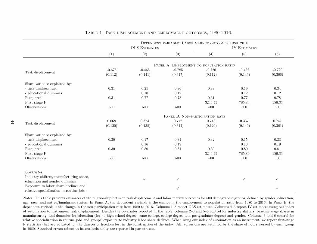
Table 4: Task displacement and employment outcomes, 1980-2016.

Dependent variable: Labor market outcomes 1980–2016OLS Estimates IV Estimates

(1) (2) (3) (4) (5) (6)

Panel A. Employment to population ratio

Task displacement-0.676 -0.465 -0.785 -0.720 -0.422 -0.729(0.112) (0.141) (0.317) (0.112) (0.149) (0.366)

Share variance explained by:- task displacement 0.31 0.21 0.36 0.33 0.19 0.34- educational dummies 0.10 0.12 0.12 0.12R-squared 0.31 0.77 0.78 0.31 0.77 0.78First-stage F 3246.45 785.80 156.33Observations 500 500 500 500 500 500

Panel B. Non-participation rate

Task displacement0.668 0.374 0.772 0.718 0.337 0.747

(0.120) (0.138) (0.312) (0.120) (0.149) (0.361)

Share variance explained by:- task displacement 0.30 0.17 0.34 0.32 0.15 0.33- educational dummies 0.16 0.19 0.18 0.19R-squared 0.30 0.80 0.81 0.30 0.80 0.81First-stage F 3246.45 785.80 156.33Observations 500 500 500 500 500 500

Covariates:Industry shifters, manufacturing share,education and gender dummies

✓ ✓ ✓ ✓

Exposure to labor share declines andrelative specialization in routine jobs

✓ ✓

Notes: This table presents estimates of the relationship between task displacement and labor market outcomes for 500 demographic groups, defined by gender, education,age, race, and native/immigrant status. In Panel A, the dependent variable is the change in the employment to population ratio from 1980 to 2016. In Panel B, thedependent variable is the change in the non-participation rate from 1980 to 2016. Columns 1–3 report OLS estimates. Columns 4–6 report IV estimates using our indexof automation to instrument task displacement. Besides the covariates reported in the table, columns 2–3 and 5–6 control for industry shifters, baseline wage shares inmanufacturing, and dummies for education (for no high school degree, some college, college degree and postgraduate degree) and gender. Columns 3 and 6 control forrelative specialization in routine jobs and groups’ exposure to industry labor share declines. When using our index of automation as an instrument, we report first-stageF statistics that are adjusted for the degrees of freedom lost in the construction of the index. All regressions are weighted by the share of hours worked by each groupin 1980. Standard errors robust to heteroskedasticity are reported in parentheses.

44

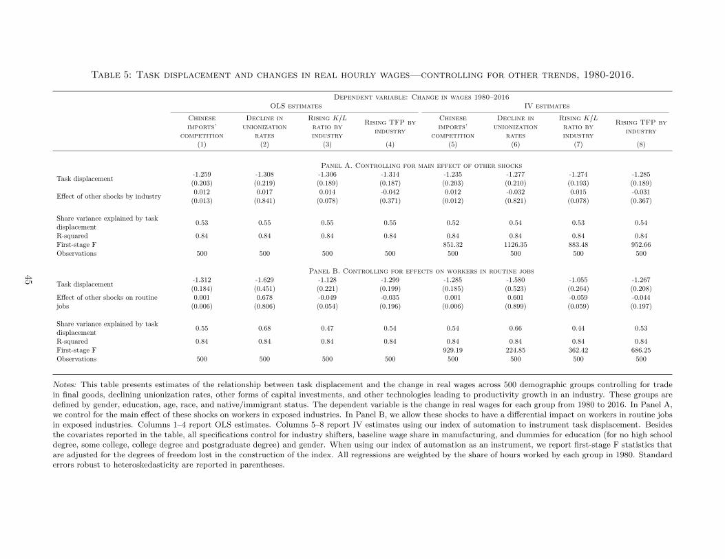
Table 5: Task displacement and changes in real hourly wages—controlling for other trends, 1980-2016.

Dependent variable: Change in wages 1980–2016OLS estimates IV estimates

Chineseimports’

competition

Decline inunionization

rates

Rising K/Lratio byindustry

Rising TFP byindustry

Chineseimports’

competition

Decline inunionization

rates

Rising K/Lratio byindustry

Rising TFP byindustry

(1) (2) (3) (4) (5) (6) (7) (8)

Panel A. Controlling for main effect of other shocks

Task displacement-1.259 -1.308 -1.306 -1.314 -1.235 -1.277 -1.274 -1.285(0.203) (0.219) (0.189) (0.187) (0.203) (0.210) (0.193) (0.189)

Effect of other shocks by industry0.012 0.017 0.014 -0.042 0.012 -0.032 0.015 -0.031

(0.013) (0.841) (0.078) (0.371) (0.012) (0.821) (0.078) (0.367)

Share variance explained by taskdisplacement

0.53 0.55 0.55 0.55 0.52 0.54 0.53 0.54

R-squared 0.84 0.84 0.84 0.84 0.84 0.84 0.84 0.84First-stage F 851.32 1126.35 883.48 952.66Observations 500 500 500 500 500 500 500 500

Panel B. Controlling for effects on workers in routine jobs

Task displacement-1.312 -1.629 -1.128 -1.299 -1.285 -1.580 -1.055 -1.267(0.184) (0.451) (0.221) (0.199) (0.185) (0.523) (0.264) (0.208)

Effect of other shocks on routinejobs

0.001 0.678 -0.049 -0.035 0.001 0.601 -0.059 -0.044(0.006) (0.806) (0.054) (0.196) (0.006) (0.899) (0.059) (0.197)

Share variance explained by taskdisplacement

0.55 0.68 0.47 0.54 0.54 0.66 0.44 0.53

R-squared 0.84 0.84 0.84 0.84 0.84 0.84 0.84 0.84First-stage F 929.19 224.85 362.42 686.25Observations 500 500 500 500 500 500 500 500

Notes: This table presents estimates of the relationship between task displacement and the change in real wages across 500 demographic groups controlling for tradein final goods, declining unionization rates, other forms of capital investments, and other technologies leading to productivity growth in an industry. These groups aredefined by gender, education, age, race, and native/immigrant status. The dependent variable is the change in real wages for each group from 1980 to 2016. In Panel A,we control for the main effect of these shocks on workers in exposed industries. In Panel B, we allow these shocks to have a differential impact on workers in routine jobsin exposed industries. Columns 1–4 report OLS estimates. Columns 5–8 report IV estimates using our index of automation to instrument task displacement. Besidesthe covariates reported in the table, all specifications control for industry shifters, baseline wage share in manufacturing, and dummies for education (for no high schooldegree, some college, college degree and postgraduate degree) and gender. When using our index of automation as an instrument, we report first-stage F statistics thatare adjusted for the degrees of freedom lost in the construction of the index. All regressions are weighted by the share of hours worked by each group in 1980. Standarderrors robust to heteroskedasticity are reported in parentheses.

45

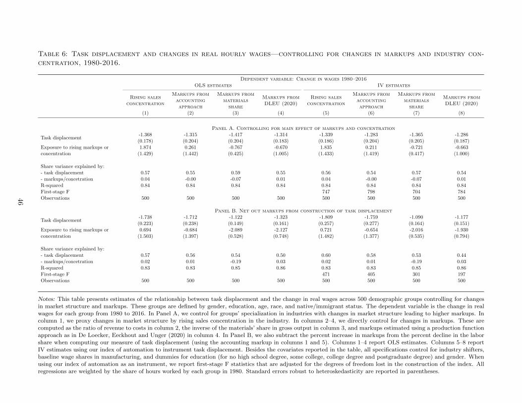
Table 6: Task displacement and changes in real hourly wages—controlling for changes in markups and industry con-centration, 1980-2016.

Dependent variable: Change in wages 1980–2016OLS estimates IV estimates

Rising salesconcentration

Markups fromaccountingapproach

Markups frommaterials

share

Markups fromDLEU (2020)

Rising salesconcentration

Markups fromaccountingapproach

Markups frommaterials

share

Markups fromDLEU (2020)

(1) (2) (3) (4) (5) (6) (7) (8)

Panel A. Controlling for main effect of markups and concentration

Task displacement-1.368 -1.315 -1.417 -1.314 -1.339 -1.283 -1.365 -1.286(0.178) (0.204) (0.204) (0.183) (0.186) (0.204) (0.205) (0.187)

Exposure to rising markups orconcentration

1.874 0.261 -0.767 -0.670 1.835 0.211 -0.721 -0.663(1.429) (1.442) (0.425) (1.005) (1.433) (1.419) (0.417) (1.000)

Share variance explained by:- task displacement 0.57 0.55 0.59 0.55 0.56 0.54 0.57 0.54- markups/concetration 0.04 -0.00 -0.07 0.01 0.04 -0.00 -0.07 0.01R-squared 0.84 0.84 0.84 0.84 0.84 0.84 0.84 0.84First-stage F 747 798 704 784Observations 500 500 500 500 500 500 500 500

Panel B. Net out markups from construction of task displacement

Task displacement-1.738 -1.712 -1.122 -1.323 -1.809 -1.759 -1.090 -1.177(0.223) (0.238) (0.149) (0.161) (0.257) (0.277) (0.164) (0.151)

Exposure to rising markups orconcentration

0.694 -0.684 -2.089 -2.127 0.721 -0.654 -2.016 -1.930(1.503) (1.397) (0.528) (0.748) (1.482) (1.377) (0.535) (0.794)

Share variance explained by:- task displacement 0.57 0.56 0.54 0.50 0.60 0.58 0.53 0.44- markups/concetration 0.02 0.01 -0.19 0.03 0.02 0.01 -0.19 0.03R-squared 0.83 0.83 0.85 0.86 0.83 0.83 0.85 0.86First-stage F 471 405 301 197Observations 500 500 500 500 500 500 500 500

Notes: This table presents estimates of the relationship between task displacement and the change in real wages across 500 demographic groups controlling for changesin market structure and markups. These groups are defined by gender, education, age, race, and native/immigrant status. The dependent variable is the change in realwages for each group from 1980 to 2016. In Panel A, we control for groups’ specialization in industries with changes in market structure leading to higher markups. Incolumn 1, we proxy changes in market structure by rising sales concentration in the industry. In columns 2–4, we directly control for changes in markups. These arecomputed as the ratio of revenue to costs in column 2, the inverse of the materials’ share in gross output in column 3, and markups estimated using a production functionapproach as in De Loecker, Eeckhout and Unger (2020) in column 4. In Panel B, we also subtract the percent increase in markups from the percent decline in the laborshare when computing our measure of task displacement (using the accounting markup in columns 1 and 5). Columns 1–4 report OLS estimates. Columns 5–8 reportIV estimates using our index of automation to instrument task displacement. Besides the covariates reported in the table, all specifications control for industry shifters,baseline wage shares in manufacturing, and dummies for education (for no high school degree, some college, college degree and postgraduate degree) and gender. Whenusing our index of automation as an instrument, we report first-stage F statistics that are adjusted for the degrees of freedom lost in the construction of the index. Allregressions are weighted by the share of hours worked by each group in 1980. Standard errors robust to heteroskedasticity are reported in parentheses.

46

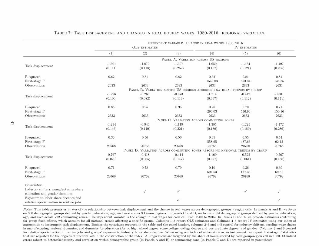
Table 7: Task displacement and changes in real hourly wages, 1980-2016: regional variation.

Dependent variable: Change in real wages 1980–2016OLS estimates IV estimates

(1) (2) (3) (4) (5) (6)

Panel A. Variation across US regions

Task displacement-1.601 -1.070 -1.307 -1.650 -1.134 -1.497(0.111) (0.118) (0.252) (0.107) (0.121) (0.285)

R-squared 0.62 0.81 0.82 0.62 0.81 0.81First-stage F 1548.83 893.34 146.35Observations 2633 2633 2633 2633 2633 2633

Panel B. Variation across US regions absorbing national trends by group

Task displacement-1.296 -0.263 -0.373 -1.714 -0.412 -0.601(0.100) (0.082) (0.119) (0.097) (0.112) (0.171)

R-squared 0.88 0.95 0.95 0.26 0.70 0.71First-stage F 293.03 546.96 150.16Observations 2633 2633 2633 2633 2633 2633

Panel C. Variation across commuting zones

Task displacement-1.234 -0.943 -1.119 -1.385 -1.225 -1.472(0.146) (0.140) (0.221) (0.189) (0.180) (0.286)

R-squared 0.36 0.56 0.56 0.35 0.55 0.54First-stage F 558.65 487.63 92.12Observations 20768 20768 20768 20768 20768 20768

Panel D. Variation across commuting zones absorbing national trends by group

Task displacement-0.767 -0.418 -0.414 -1.169 -0.522 -0.567(0.070) (0.065) (0.147) (0.097) (0.061) (0.188)

R-squared 0.71 0.78 0.79 0.10 0.36 0.39First-stage F 694.53 137.33 69.31Observations 20768 20768 20768 20768 20768 20768

Covariates:Industry shifters, manufacturing share,education and gender dummies

✓ ✓ ✓ ✓

Exposure to labor share declines andrelative specialization in routine jobs

✓ ✓

Notes: This table presents estimates of the relationship between task displacement and the change in real wages across demographic groups × region cells. In panels A and B, we focuson 300 demographic groups defined by gender, education, age, and race across 9 Census regions. In panels C and D, we focus on 54 demographic groups defined by gender, education,age, and race across 722 commuting zones. The dependent variable is the change in real wages for each cell from 1980 to 2016. In Panels B and D we provide estimates controllingfor group fixed effects, which account for all national trends affecting a specific group. Columns 1–3 report OLS estimates and Columns 4–6 report IV estimates using our index ofautomation to instrument task displacement. Besides the covariates reported in the table and the panel headers, columns 2–3 and 4–5 control for industry shifters, baseline wage sharesin manufacturing, regional dummies, and dummies for education (for no high school degree, some college, college degree and postgraduate degree) and gender. Columns 3 and 6 controlfor relative specialization in routine jobs and groups’ exposure to industry labor share decline. When using our index of automation as an instrument, we report first-stage F statisticsthat are adjusted for the degrees of freedom lost in the construction of the index. All regressions are weighted by the share of hours worked by each group-region cell in 1980. Standarderrors robust to heteroskedasticity and correlation within demographic group (in Panels A and B) or commuting zone (in Panels C and D) are reported in parentheses.

47

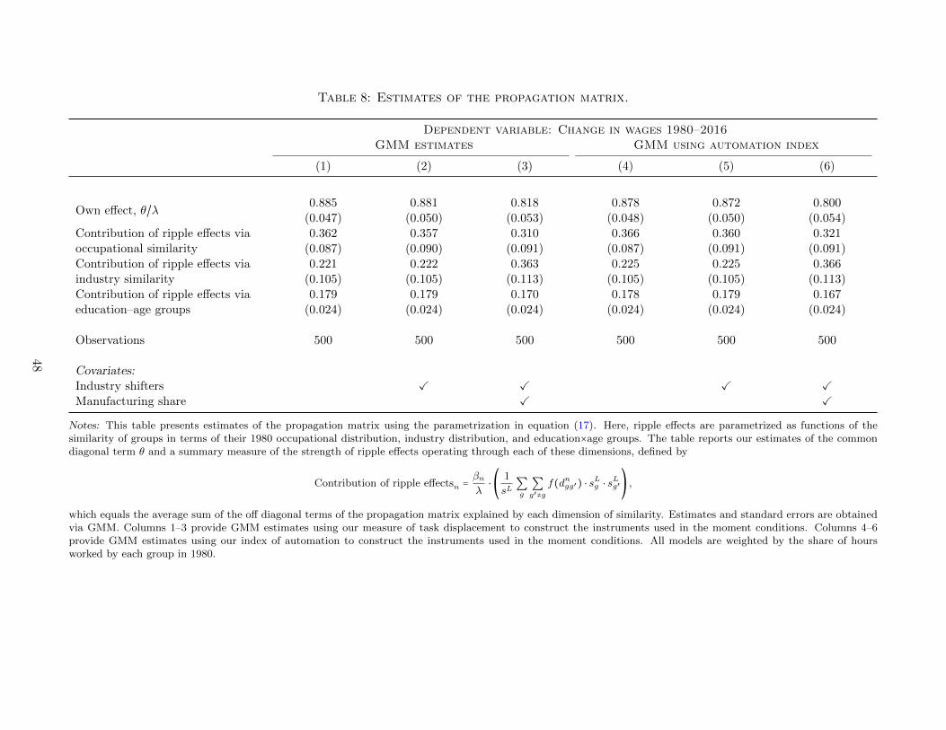
Table 8: Estimates of the propagation matrix.

Dependent variable: Change in wages 1980–2016GMM estimates GMM using automation index

(1) (2) (3) (4) (5) (6)

Own effect, θ/λ0.885 0.881 0.818 0.878 0.872 0.800

(0.047) (0.050) (0.053) (0.048) (0.050) (0.054)Contribution of ripple effects viaoccupational similarity

0.362 0.357 0.310 0.366 0.360 0.321(0.087) (0.090) (0.091) (0.087) (0.091) (0.091)

Contribution of ripple effects viaindustry similarity

0.221 0.222 0.363 0.225 0.225 0.366(0.105) (0.105) (0.113) (0.105) (0.105) (0.113)

Contribution of ripple effects viaeducation–age groups

0.179 0.179 0.170 0.178 0.179 0.167(0.024) (0.024) (0.024) (0.024) (0.024) (0.024)

Observations 500 500 500 500 500 500

Covariates:Industry shifters ✓ ✓ ✓ ✓

Manufacturing share ✓ ✓

Notes: This table presents estimates of the propagation matrix using the parametrization in equation (17). Here, ripple effects are parametrized as functions of thesimilarity of groups in terms of their 1980 occupational distribution, industry distribution, and education×age groups. The table reports our estimates of the commondiagonal term θ and a summary measure of the strength of ripple effects operating through each of these dimensions, defined by

Contribution of ripple effectsn =βnλ⋅⎛⎝

1

sL∑g

∑g′≠g

f(dngg′) ⋅ sLg ⋅ sLg′⎞⎠,

which equals the average sum of the off diagonal terms of the propagation matrix explained by each dimension of similarity. Estimates and standard errors are obtainedvia GMM. Columns 1–3 provide GMM estimates using our measure of task displacement to construct the instruments used in the moment conditions. Columns 4–6provide GMM estimates using our index of automation to construct the instruments used in the moment conditions. All models are weighted by the share of hoursworked by each group in 1980.

48

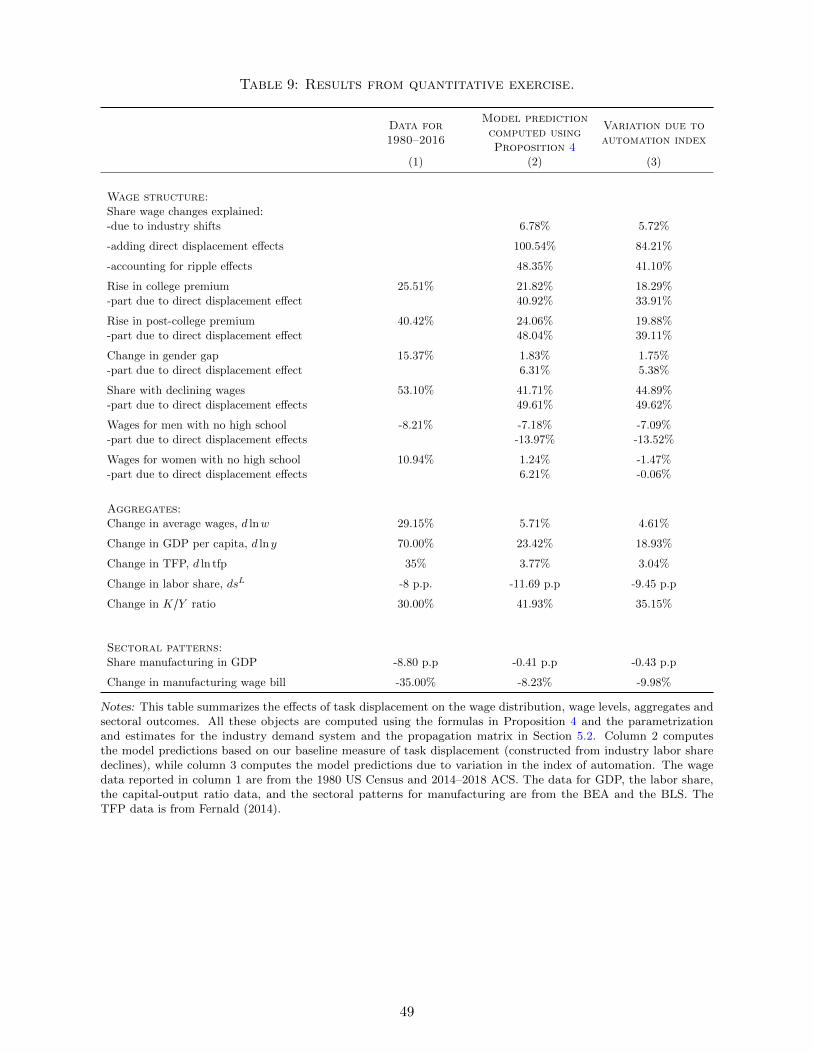
Table 9: Results from quantitative exercise.

Data for1980–2016

Model predictioncomputed usingProposition 4

Variation due toautomation index

(1) (2) (3)

Wage structure:Share wage changes explained:-due to industry shifts 6.78% 5.72%

-adding direct displacement effects 100.54% 84.21%

-accounting for ripple effects 48.35% 41.10%

Rise in college premium 25.51% 21.82% 18.29%-part due to direct displacement effect 40.92% 33.91%

Rise in post-college premium 40.42% 24.06% 19.88%-part due to direct displacement effect 48.04% 39.11%

Change in gender gap 15.37% 1.83% 1.75%-part due to direct displacement effect 6.31% 5.38%

Share with declining wages 53.10% 41.71% 44.89%-part due to direct displacement effects 49.61% 49.62%

Wages for men with no high school -8.21% -7.18% -7.09%-part due to direct displacement effects -13.97% -13.52%

Wages for women with no high school 10.94% 1.24% -1.47%-part due to direct displacement effects 6.21% -0.06%

Aggregates:Change in average wages, d lnw 29.15% 5.71% 4.61%

Change in GDP per capita, d ln y 70.00% 23.42% 18.93%

Change in TFP, d ln tfp 35% 3.77% 3.04%

Change in labor share, dsL -8 p.p. -11.69 p.p -9.45 p.p

Change in K/Y ratio 30.00% 41.93% 35.15%

Sectoral patterns:Share manufacturing in GDP -8.80 p.p -0.41 p.p -0.43 p.p

Change in manufacturing wage bill -35.00% -8.23% -9.98%

Notes: This table summarizes the effects of task displacement on the wage distribution, wage levels, aggregates andsectoral outcomes. All these objects are computed using the formulas in Proposition 4 and the parametrizationand estimates for the industry demand system and the propagation matrix in Section 5.2. Column 2 computesthe model predictions based on our baseline measure of task displacement (constructed from industry labor sharedeclines), while column 3 computes the model predictions due to variation in the index of automation. The wagedata reported in column 1 are from the 1980 US Census and 2014–2018 ACS. The data for GDP, the labor share,the capital-output ratio data, and the sectoral patterns for manufacturing are from the BEA and the BLS. TheTFP data is from Fernald (2014).

49

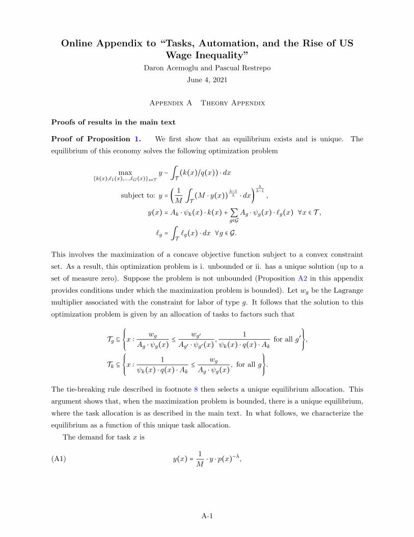
Online Appendix to “Tasks, Automation, and the Rise of USWage Inequality”

Daron Acemoglu and Pascual Restrepo

June 4, 2021

Appendix A Theory Appendix

Proofs of results in the main text

Proof of Proposition 1. We first show that an equilibrium exists and is unique. The

equilibrium of this economy solves the following optimization problem

max{k(x),`1(x),...,`G(x)}x∈T

y − ∫T(k(x)/q(x)) ⋅ dx

subject to: y = (1

M∫T(M ⋅ y(x))

λ−1λ ⋅ dx)

λλ−1

,

y(x) = Ak ⋅ ψk(x) ⋅ k(x) +∑g∈G

Ag ⋅ ψg(x) ⋅ `g(x) ∀x ∈ T ,

`g = ∫T`g(x) ⋅ dx ∀g ∈ G.

This involves the maximization of a concave objective function subject to a convex constraint

set. As a result, this optimization problem is i. unbounded or ii. has a unique solution (up to a

set of measure zero). Suppose the problem is not unbounded (Proposition A2 in this appendix

provides conditions under which the maximization problem is bounded). Let wg be the Lagrange

multiplier associated with the constraint for labor of type g. It follows that the solution to this

optimization problem is given by an allocation of tasks to factors such that

Tg ⊆

⎧⎪⎪⎨⎪⎪⎩

x ∶wg

Ag ⋅ ψg(x)≤

wg′

Ag′ ⋅ ψg′(x),

1

ψk(x) ⋅ q(x) ⋅Akfor all g′

⎫⎪⎪⎬⎪⎪⎭

,

Tk ⊆

⎧⎪⎪⎨⎪⎪⎩

x ∶1

ψk(x) ⋅ q(x) ⋅Ak≤

wg

Ag ⋅ ψg(x), for all g

⎫⎪⎪⎬⎪⎪⎭

.

The tie-breaking rule described in footnote 8 then selects a unique equilibrium allocation. This

argument shows that, when the maximization problem is bounded, there is a unique equilibrium,

where the task allocation is as described in the main text. In what follows, we characterize the

equilibrium as a function of this unique task allocation.

The demand for task x is

y(x) =1

M⋅ y ⋅ p(x)−λ,(A1)

A-1

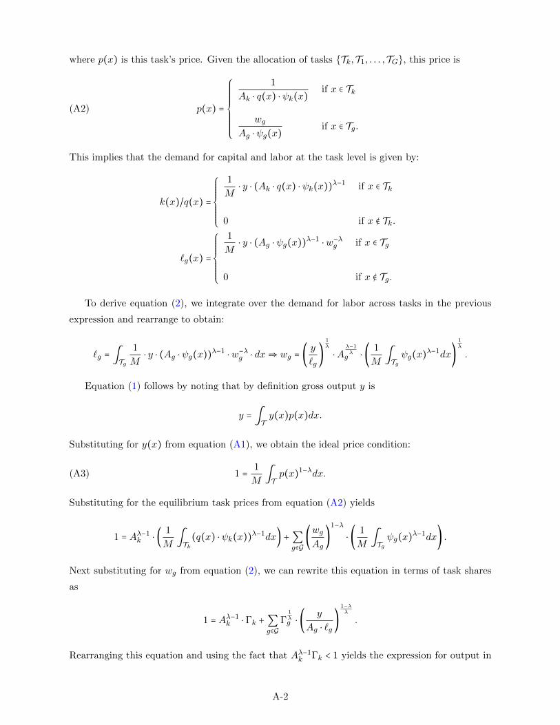
where p(x) is this task’s price. Given the allocation of tasks {Tk,T1, . . . ,TG}, this price is

p(x) =

⎧⎪⎪⎪⎪⎪⎪⎪⎪⎨⎪⎪⎪⎪⎪⎪⎪⎪⎩

1

Ak ⋅ q(x) ⋅ ψk(x)if x ∈ Tk

wg

Ag ⋅ ψg(x)if x ∈ Tg.

(A2)

This implies that the demand for capital and labor at the task level is given by:

k(x)/q(x) =

⎧⎪⎪⎪⎪⎪⎪⎨⎪⎪⎪⎪⎪⎪⎩

1

M⋅ y ⋅ (Ak ⋅ q(x) ⋅ ψk(x))

λ−1 if x ∈ Tk

0 if x ∉ Tk.

`g(x) =

⎧⎪⎪⎪⎪⎪⎪⎨⎪⎪⎪⎪⎪⎪⎩

1

M⋅ y ⋅ (Ag ⋅ ψg(x))

λ−1⋅w−λ

g if x ∈ Tg

0 if x ∉ Tg.

To derive equation (2), we integrate over the demand for labor across tasks in the previous

expression and rearrange to obtain:

`g = ∫Tg

1

M⋅ y ⋅ (Ag ⋅ ψg(x))

λ−1⋅w−λ

g ⋅ dx⇒ wg = (y

`g)

1λ

⋅Aλ−1λg ⋅ (

1

M∫Tg

ψg(x)λ−1dx)

1λ

.

Equation (1) follows by noting that by definition gross output y is

y = ∫Ty(x)p(x)dx.

Substituting for y(x) from equation (A1), we obtain the ideal price condition:

1 =1

M∫Tp(x)1−λdx.(A3)

Substituting for the equilibrium task prices from equation (A2) yields

1 = Aλ−1k ⋅ (

1

M∫Tk

(q(x) ⋅ ψk(x))λ−1dx) +∑

g∈G

(wg

Ag)

1−λ

⋅ (1

M∫Tg

ψg(x)λ−1dx) .

Next substituting for wg from equation (2), we can rewrite this equation in terms of task shares

as

1 = Aλ−1k ⋅ Γk +∑

g∈G

Γ1λg ⋅ (

y

Ag ⋅ `g)

1−λλ

.

Rearranging this equation and using the fact that Aλ−1k Γk < 1 yields the expression for output in

A-2

equation (1).

Finally, we can compute factor shares as:

sK =1

M∫Tk

y ⋅ p(x)1−λdx/y = Aλ−1k ⋅ Γk.

Because of constant-returns to scale, we must have sL = 1 − sK .

To conclude, note that in any competitive equilibrium we have sL, sK ∈ [0,1], and so

1 ≥ Aλ−1k ⋅ Γk,

as claimed in the main text.

Proof of Proposition 2. We now characterize the effects of a small change in technology. As

in the text, we use Dg ⊂ Tg to denote the set of tasks that used to be performed by group g and

where, after the technological change, capital now outperforms labor. The definitions of d ln Γdeepg

and d ln Γdispg in the main text imply

d ln Γg = (λ − 1)d ln Γdeepg − d ln Γdisp

g .(A4)

To characterize the effects of technology on wages, we first log-differentiate equation (2):

d lnwg =1

λd ln y +

λ − 1

λd lnAg +

1

λd ln Γg.

Plugging the formula for d ln Γg in (A4) yields the expression for wage changes in (4).

Let us next define changes in TFP, which are:

d ln TFP = d ln y − sK ⋅ d lnk,

where k = ∫Tkk(x)/q(x)dx. This definition corresponds to gross TFP, defined as the change in

gross output that is not explain by the change in capital and intermediate inputs, k. This can

also be written in its dual representation as:

d ln TFP = ∑g∈G

sLg ⋅ d lnwg − ∫Tk

sK(x)d ln q(x)dx,(A5)

where sK(x) denotes the share of capital k(x) in gross output and sLg denote the share of labor

of type g in gross output.

To obtain this expression, note that because of constant returns to scale, Euler’s theorem

A-3

implies

y = ∑g∈G

wg`g + ∫Tk

k(x)/q(x)dx.

For any small change in technology, we have

d ln y = ∑g∈G

sLg ⋅ d lnwg + ∫Tk

sK(x)d lnk(x)dx − ∫Tk

sK(x)d ln q(x)dx +1

y∑g∈G∫Dg

(knew(x)/qnew

(x))dx,

where the knew(x) and qnew(x) denote the new capital usage and prices in the newly-automated

tasks. Rearranging, we have

d ln y −⎛

⎝∫Tk

sK(x)d lnk(x)dx +1

y∑g∈G∫Dg

(knew(x)/qnew

(x))dx⎞

⎠= ∑g∈G

sLg ⋅ d lnwg − ∫Tk

sK(x)d ln q(x)dx.

Finally, using the fact that

sKd lnk =1

ydk = ∫

Tk

sK(x)d lnk(x)dx +1

y∑g∈G∫Dg

(knew(x)/qnew

(x))dx,

we obtain the dual representation of TFP.

We now return to determining the contribution of different types of technologies to TFP. For

this, we use the ideal price index condition in equation (A3), which we can rewrite as

1 = Aλ−1k ⋅ (

1

M∫Tk

(q(x) ⋅ ψk(x))λ−1dx) +∑

g∈G

(wg

Ag)

1−λ

⋅ (1

M∫Tg

ψg(x)λ−1dx) .

Log-differentiating this equation following an arbitrary change in technology and capital prices,

we obtain:

∑g∈G

sLg ⋅ d lnwg − ∫Tk

sK(x)d ln q(x)dx =sK ⋅ (d lnAk + d ln Γdeepk )(A6)

+∑g∈G

sLg ⋅ (d lnAg + d ln Γdeepg )

+1

λ − 1

⎡⎢⎢⎢⎢⎣

sK ⋅ d ln Γdispk −∑

g∈G

sLg ⋅ d ln Γdispg

⎤⎥⎥⎥⎥⎦

.

Let us define the last line as

∆ =1

λ − 1

⎡⎢⎢⎢⎢⎣

sK ⋅ d ln Γdispk −∑

g∈G

sLg ⋅ d ln Γdispg

⎤⎥⎥⎥⎥⎦

,

which represents the reallocation of tasks from labor to capital.

To develop this expression further, let us recall the definition of the cost-saving gains from

A-4

automating task x:

πg(x) =1

λ − 1

⎡⎢⎢⎢⎢⎣

(wgAk ⋅ q(x) ⋅ ψk(x)

Ag ⋅ ψg(x))

λ−1

− 1

⎤⎥⎥⎥⎥⎦

> 0.

Averaging this across tasks, we obtain the average cost-saving gains from automating tasks in Dg

(which was also defined in the text):

πg =1

M∫Dg

ψg(x)λ−1

⋅ πg(x)dx/1

M∫Dg

ψg(x)λ−1dx.

Using these definitions, ∆ can be rewritten as

∆ =∑g∈G

1

λ − 1

⎡⎢⎢⎢⎢⎣

Aλ−1k ⋅

1

M∫Dg

(q(x) ⋅ ψk(x))λ−1dx − (

wg

Ag)

1−λ

⋅1

M∫Dg

ψg(x)λ−1dx

⎤⎥⎥⎥⎥⎦

=∑g∈G

1

M∫Dg

1

λ − 1

⎡⎢⎢⎢⎢⎣

(Ak ⋅ q(x) ⋅ ψk(x))λ−1

− (wg

Ag)

1−λ

⋅ ψg(x)λ−1

⎤⎥⎥⎥⎥⎦

dx

=∑g∈G

1

M∫Dg

(wg

Ag)

1−λ

⋅ ψg(x)λ−1

⋅ πg(x)dx

=∑g∈G

(wg

Ag)

1−λ

⋅ (1

M∫Dg

ψg(x)λ−1dx) ⋅ πg.

Next, using the fact that sLg = (wgAg

)1−λ

⋅ ( 1M ∫Tg ψg(x)

λ−1dx), we can rewrite ∆ as:

∆ = ∑g∈G

sLg ⋅

1

M∫Dg

ψg(x)λ−1dx

1

M∫Tg

ψg(x)λ−1dx

⋅ πg = ∑g∈G

sLg ⋅ d ln Γdispg ⋅ πg.

Substituting this expression for ∆ into equation (A6) and using the dual representation of

TFP in equation (A5), we obtain the TFP expressions in equation (5) as desired.

The output equation, (7), can be obtained from the TFP equation, (5). Note that by definition

we have

d ln y = d ln TFP + sK ⋅ d lnk.

Moreover, k = sK ⋅ y, which implies

d lnk = d ln sK + d ln y.

A-5

Combining these two equations yields

d ln y =1

1 − sK(d ln TFP + sK ⋅ d ln sK)

d lnk =1

1 − sK(d ln TFP + d ln sK) .

To obtain the factor share changes, note that

d ln sK = (λ − 1) ⋅ (d lnAk + d ln Γdeepk ) + d ln Γdisp

k ,

which follows from the fact that sK = Aλ−1k ⋅ Γk. We can rewrite this expression as follows:

d ln sK =(λ − 1) ⋅ (d lnAk + d ln Γdeepk ) +

1

sK⋅⎛

⎝(λ − 1) ⋅∆ +∑

g∈G

sLg ⋅ d ln Γdispg

⎞

⎠

=(λ − 1) ⋅ (d lnAk + d ln Γdeepk ) +

1

sK⋅∑g∈G

sLg ⋅ d ln Γdispg ⋅ (1 + (λ − 1) ⋅ πg),

which yields equation (6) in the proposition.

Proof of Proposition 3. We first show that an equilibrium exists and is unique. Denote

the aggregator of industry output by H(y1, . . . , yI). The equilibrium of this economy solves the

following optimization problem

max{k(x),`1(x),...,`G(x)}x∈Ti,i∈I

H(y1, . . . , yI) − ∫T(k(x)/q(x)) ⋅ dx

subject to: yi = (1

M∫T(M ⋅ y(x))

λ−1λ ⋅ dx)

λλ−1

∀i ∈ I,

y(x) = Ak ⋅ ψk(x) ⋅ k(x) +∑g∈G

Ag ⋅ ψg(x) ⋅ `g(x) ∀x ∈ T ,

`g = ∫T`g(x) ⋅ dx ∀g ∈ G.

This involves the maximization of a concave objective function subject to a convex constraint

set. As a result, this optimization problem is i. unbounded or ii. has a unique solution (up to a

set of measure zero). Suppose the problem is not unbounded (Proposition A2 in this appendix

provides conditions under which the maximization problem is bounded). Let wg be the Lagrange

multiplier associated with the constraint for labor of type g. It follows that the solution is given

by an allocation of tasks to factors such that

Tgi ⊆

⎧⎪⎪⎨⎪⎪⎩

x ∶wg

Agi ⋅ ψg(x)≤

wg′

Ag′i ⋅ ψg′(x),

1

ψk(x) ⋅ q(x) ⋅Akifor all g′

⎫⎪⎪⎬⎪⎪⎭

,

Tki ⊆

⎧⎪⎪⎨⎪⎪⎩

x ∶1

ψk(x) ⋅ q(x) ⋅Aki≤

wg

Agi ⋅ ψg(x), for all g

⎫⎪⎪⎬⎪⎪⎭

.

A-6

The tie-breaking rule described in footnote 8 then selects a unique equilibrium allocation. This

argument shows that, when the maximization problem is bounded, there is a unique equilibrium,

where the task allocation is as described in the main text. In what follows, we characterize the

equilibrium as a function of this unique task allocation (we provide a sufficient condition for finite

output at the end of the proof).

The demand for task x in sector i is

y(x) =1

Mi⋅ y ⋅ sYi (p) ⋅ p(x)−λ ⋅ (Aipi)

λ−1.

Given {Tki,T1i, . . . ,TGi}, the price of task x is

p(x) =

⎧⎪⎪⎪⎪⎪⎪⎪⎪⎨⎪⎪⎪⎪⎪⎪⎪⎪⎩

1

Ak ⋅ q(x) ⋅ ψk(x)if x ∈ Tki

wg

Ag ⋅ ψk(x)if x ∈ Tgi.

The demand for capital and labor at task x can be written as

k(x)/q(x) =

⎧⎪⎪⎪⎪⎪⎪⎨⎪⎪⎪⎪⎪⎪⎩

1

Mi⋅ y ⋅ sYi (p) ⋅ (Aipi)

λ−1⋅ (Ak ⋅ q(x) ⋅ ψk(x))

λ−1 if x ∈ Tki

0 if x ∉ Tk.

`g(x) =

⎧⎪⎪⎪⎪⎪⎪⎨⎪⎪⎪⎪⎪⎪⎩

1

Mi⋅ y ⋅ sYi (p) ⋅ (Aipi)

λ−1⋅ (Ag ⋅ ψg(x))

λ−1⋅w−λ

g if x ∈ Tg

0 if x ∉ Tg.

Integrating these demands, as in the proof of Proposition 1, and rearranging, we have

`g =∑i∈I∫Tgi

1

Mi⋅ y ⋅ sYi (p) ⋅ (Aipi)

λ−1⋅ (Ag ⋅ ψg(x))

λ−1⋅w−λ

g ⋅ dx

⇒ wg = (y

`g)

1λ

⋅Aλ−1λg ⋅ (∑

i∈I

sYi (p) ⋅ (Aipi)λ−1

⋅1

Mi∫Tgi

ψg(x)λ−1dx)

1λ

,

which thus establishes equation (8) as desired.

To derive the industry price index in equation (9), we observe that

pi ⋅ yi = ∫Ti

p(x) ⋅ y(x)dx⇒ pi =1

Ai(

1

Mi∫Ti

p(x)1−λdx)

11−λ

.

A-7

Using the allocation of tasks {Tki,T1i, . . . ,TGi}, this implies

pi =1

Ai(

1

Mi∫Ti

p(x)1−λdx)

11−λ

=1

Ai

⎛

⎝Ak ⋅ (

1

Mi∫Tki

(q(x) ⋅ ψk(x))λ−1dx) +∑

g∈G

w1−λg ⋅Aλ−1

g ⋅ (1

Mi∫Tgi

ψg(x)λ−1dx)

⎞

⎠

11−λ

,

which yields equation (10) in the proposition.

Finally, because industry shares must add up to 1, equation (10) holds, completing the proof.

Although not reported, factor shares can be computed as

sK =Aλ−1k ⋅∑

i∈I

sYi (p) ⋅ (Aipi)λ−1

⋅ Γki(A7)

sL =1 −Aλ−1k ⋅∑

i∈I

sYi (p) ⋅ (Aipi)λ−1

⋅ Γki.(A8)

Proof of Proposition 4. We first provide a proof for the existence and some of the properties

of the propagation matrix Θ.

Define the matrix

Σ = 1 −1

λ

∂ ln Γ(w,ζ,Ψ)

∂ lnw.

This matrix satisfies several properties. First, because ∂Γg/∂wg′ ≥ 0, all of its off-diagonal entries

are negative. This implies that Σ is a Z−matrix.

Second, Σ has a positive dominant diagonal. This follows from the fact that

Σgg = 1 −1

λ

∂ ln Γg

∂ lnwg> 0,

and

Σgg − ∑g′≠g

∣Σgg′ ∣ = 1 −∑g′

1

λ

∂ ln Γg

∂ lnwg′> 1.

This last inequality follows from the fact that ∑g′∂ ln Γg∂ lnwg′

≤ 0, which is true since when all wages

rise by the same amount, workers lose tasks to capital but do not experience task reallocation

among them.

Third, all eigenvalues of Σ have a real part that exceeds 1. This follows from an application of

Gershgorin circle theorem, which states that for each eigenvalue ε of Σ, we can find a dimension

g such that

∣∣ε −Σgg ∣∣ < ∑g′≠g

∣Σgg′ ∣.

A-8

This inequality requires that

R(ε) ∈

⎡⎢⎢⎢⎢⎣

Σgg − ∑g′≠g

∣Σgg′ ∣,Σgg + ∑g′≠g

∣Σgg′ ∣

⎤⎥⎥⎥⎥⎦

.

Because Σgg −∑g′≠g ∣Σgg′ ∣ > 1 for all g, as shown above, all eigenvalues of Σ have a real part that

is greater than 1.

Fourth, since Σ has negative off diagonal elements and all of its eigenvalues have a positive

real part, we can conclude that it is an M−matrix.

Because Σ is an M−matrix, its inverse Θ exists and has positive and real entries, θgg′ ≥ 0, as

desired. Moreover, each eigenvalue of Θ has a real part that is positive and less than 1. Finally,

the row and column sums of Θ are also less than 1. In particular, denote by θrg the sum of the

elements of row g of Θ. Then:

Θ ⋅ (1,1, . . . ,1)′1 = (θr1, θr2, . . . , θ

rG)

′⇒ Σ ⋅ (θr1, θ

r2, . . . , θ

rG)

′= (1,1, . . . ,1)′.

This equality requires that

Σgg ⋅ θrg + ∑

g′≠g

Σgg′ ⋅ θrg′ = 1.

Now, suppose without loss of generality, that θr1 > θr2 > . . . > θrG > 0 (all rows must have strictly

positive sums, since θgg′ = 0 for all g′ would imply that Θ is singular, contradicting the fact that

all its eigenavlues have real parts in (0,1)). We have

Σ11 ⋅ θr1 + ∑

g′≠1

Σ1g′ ⋅ θrg′ = 1,

which implies that

(1 −1

λ

∂ ln Γ1

d lnw1) ⋅ θr1 = 1 +

1

λ∑g′≠1

∂ ln Γ1

d lnwg′⋅ θrg′ ≤ 1 +

1

λ∑g′≠1

∂ ln Γ1

d lnwg′⋅ θr1.

Because ∑g′∂ ln Γ1

d lnwg′≤ 0, we can rewrite this inequality as

θr1 < 1 +1

λ∑g′

∂ ln Γ1

d lnwg′⋅ θr1 ≤ 1.

An identical argument establishes that column sums of Θ lie in (0,1).

Having introduced the propagation matrix Θ, we are now in a position to derive the formulas

characterizing the effects of technology on wages, sectoral prices, and TFP.

First, define weg = wg/Ag as the wage per efficiency unit of labor of g workers. Equation (8)

A-9

then implies

weg = (y

Ag ⋅ `g)

1λ

⋅ Γg(w,ζ,Ψ)1λ .

Log-differentiating this equation in response to an automation (task-displacing) technology, we

obtain:

d lnweg =1

λd ln y −

1

λd ln Γdisp

g +1

λ∑i∈I

ωgi ⋅ d ln ζi +1

λ

∂ ln Γg

∂ lnw⋅ d lnw.

Stacking these equations for all groups, we can write:

⎛⎜⎜⎜⎜⎜⎜⎝

d lnwe1

d lnwe1

...

d lnweG

⎞⎟⎟⎟⎟⎟⎟⎠

=1

λ

⎛⎜⎜⎜⎜⎜⎜⎝

d ln y

d ln y

...

d ln y

⎞⎟⎟⎟⎟⎟⎟⎠

+1

λ

⎛⎜⎜⎜⎜⎜⎜⎝

∑i∈I ω1i ⋅ d ln ζi

∑i∈I ω2i ⋅ d ln ζi

...

∑i∈I ωGi ⋅ d ln ζi

⎞⎟⎟⎟⎟⎟⎟⎠

−1

λ

⎛⎜⎜⎜⎜⎜⎜⎝

d ln Γdisp1

d ln Γdisp2

...

d ln ΓdispG

⎞⎟⎟⎟⎟⎟⎟⎠

+1

λ

∂ ln Γ

∂ lnw⋅

⎛⎜⎜⎜⎜⎜⎜⎝

d lnwe1

d lnwe1

...

d lnweG

⎞⎟⎟⎟⎟⎟⎟⎠

.

We can solve this system of equations as

⎛⎜⎜⎜⎜⎜⎜⎝

d lnwe1

d lnwe1

...

d lnweG

⎞⎟⎟⎟⎟⎟⎟⎠

=1

λΘ ⋅

⎛⎜⎜⎜⎜⎜⎜⎝

d ln y

d ln y

...

d ln y

⎞⎟⎟⎟⎟⎟⎟⎠

+1

λΘ ⋅

⎛⎜⎜⎜⎜⎜⎜⎝

∑i∈I ω1i ⋅ d ln ζi

∑i∈I ω2i ⋅ d ln ζi

...

∑i∈I ωGi ⋅ d ln ζi

⎞⎟⎟⎟⎟⎟⎟⎠

−1

λΘ ⋅

⎛⎜⎜⎜⎜⎜⎜⎝

d ln Γdisp1

d ln Γdisp2

...

d ln ΓdispG

⎞⎟⎟⎟⎟⎟⎟⎠

,

which implies

d lnwg =εg

λd ln y +

1

λΘg ⋅ d ln ζ −

1

λΘg ⋅ d ln Γdisp,

where

d ln ζg =∑i∈I

ωgi ⋅ d ln ζi =∑i∈I

ωgi ⋅ (∂ ln sYi (p)

∂ lnp⋅ d ln p + (λ − 1) ⋅ d lnpi) .

Turning to industry prices, note that these are given by equation (10). By definition, the

equilibrium task allocation {Tki,T1i, . . . ,TGi} solves the cost-minimization problem:

pi = min{Tki,T1i,...,TGi}

1

Ai

⎛

⎝Aλ−1k ⋅ Γki +∑

g∈G

w1−λg ⋅Aλ−1

g ⋅ Γgi⎞

⎠

11−λ

.

The envelope theorem then implies that

d lnpi = ∑g∈G

sLgi ⋅ d lnwg − (Aipi)λ−1 1

λ − 1

⎡⎢⎢⎢⎢⎣

Aλ−1k ⋅ dΓdisp

ki −∑g∈G

w1−λg ⋅Aλ−1

g ⋅ dΓdispgi

⎤⎥⎥⎥⎥⎦

,

A-10

since the reallocation of tasks across factors in response to changes in factor prices has a second-

order effect on industry prices. Here, the term

∆i = (Aipi)λ−1 1

λ − 1

⎡⎢⎢⎢⎢⎣

Aλ−1k ⋅ dΓdisp

ki −∑g∈G

w1−λg ⋅Aλ−1

g ⋅ dΓdispgi

⎤⎥⎥⎥⎥⎦

is a generalization of the term ∆ in the proof of Proposition 2, and again corresponds to cost

savings from the reallocation of tasks from labor to capital, but now in industry i.

Similarly, we define the industry versions of cost savings at the task level (when tasks in the

set Dgi in industry i previous to perform by factor g are automated):

πgi(x) =1

λ − 1

⎡⎢⎢⎢⎢⎣

(wgAk ⋅ q(x) ⋅ ψk(x)

Ag ⋅ ψg(x))

λ−1

− 1

⎤⎥⎥⎥⎥⎦

> 0,

and average percent cost-saving gains in industry i as

πgi =1

Mi∫Dgi

ψg(x)λ−1

⋅ πgi(x)dx/1

Mi∫Dgi

ψg(x)λ−1dx.

Using these definitions, we can write ∆i as

∆i =(Aipi)λ−1∑g∈G

1

λ − 1

⎡⎢⎢⎢⎢⎣

Aλ−1k ⋅

1

Mi∫Dgi

(q(x) ⋅ ψk(x))λ−1dx − (

wg

Ag)

1−λ

⋅1

Mi∫Dgi

ψg(x)λ−1dx

⎤⎥⎥⎥⎥⎦

=(Aipi)λ−1∑g∈G

1

Mi∫Dgi

1

λ − 1

⎡⎢⎢⎢⎢⎣

(Ak ⋅ q(x) ⋅ ψk(x))λ−1

− (wg

Ag)

1−λ

⋅ ψg(x)λ−1

⎤⎥⎥⎥⎥⎦

dx

=(Aipi)λ−1∑g∈G

1

Mi∫Dgi

(wg

Ag)

1−λ

⋅ ψg(x)λ−1

⋅ πgi(x)dx

=(Aipi)λ−1∑g∈G

(wg

Ag)

1−λ

⋅ (1

Mi∫Dgi

ψg(x)λ−1dx) ⋅ πgi.

Again as in the proof of Proposition 2, using the fact that sLgi = (Aipi)λ−1 (

wgAg

)1−λ

⋅( 1Mi ∫Tg

ψg(x)λ−1dx),

we get

∆i = ∑g∈G

sLgi ⋅

1

Mi∫Agi

ψg(x)λ−1dx

1

Mi∫Tg

ψg(x)λ−1dx

⋅ πgi = ∑g∈G

sLgi ⋅ d ln Γdispgi ⋅ πgi,

which yields the desired formula for d lnpi in the proposition.

We now turn to TFP. As before, we use the dual definition of TFP, which now implies

d ln TFP = ∑g∈G

sLg ⋅ d lnwg.(A9)

A-11

To derive a formula for TFP, first note that given a price vector p, we can define the cost of

producing the final good as ch(p). Moreover, Shephard’s lemma implies that

sYi (p) =∂ch(p)

∂pi

pich.

Our choice of numeraire, which implies that the final good has a price of 1, then implies

1 = ch(p).

Log-differentiating this expression yields

0 =∑i∈I

sYi (p) ⋅ d lnpi

=∑i∈I

sYi (p) ⋅⎛

⎝∑g∈G

sLgi ⋅ (d lnwg − d ln Γdispgi ⋅ πgi)

⎞

⎠

=∑g∈G

sLg ⋅ d lnwg −∑i∈I

sYi (p)∑g∈G

⋅sLgi ⋅ πgi

Rearranging this expression, and using the dual definition of TFP in equation (A9), yields the

formula for the contribution of automation to TFP in the proposition.

Turning to output, the primal definition of TFP implies

d ln y = d ln TFP + sK ⋅ d lnk.

Moreover, k = sK ⋅ y, which implies

d lnk = d ln sK + d ln y.

Combining these two equations yields

d ln y =1

1 − sK(d ln TFP + sK ⋅ d ln sK)

d lnk =1

1 − sK(d ln TFP + d ln sK) .

Finally, we provide a derivation for the change in the capital share. Recall that the capital

share is given by

d ln sK = −1 − sK

sKd ln sL = −

1

sK∑g∈G

sLg ⋅ (d lnwg − d ln y) .

A-12

Additional results and lemmas

This section proves the existence of the threshold q introduced in Assumption 1 and provides

primitive conditions under which the economy will produce finite output.

Proposition A1 (Existence of q) Suppose that workers can only produce non-overlapping

sets of tasks (i.e., ψg(x) > 0 only if ψg′(x) = 0 for all g′ ≠ g). Consider the set of tasks where

capital has positive productivity, S = {x ∶ ψk(x) > 0}. Suppose that there exists ψ > 0, such that

for all x ∈ S we have ψk(x) > ψ. Then there exists a threshold q such that, if q(x) > q for all

x ∈ S, all the tasks in S are allocated to capital.

Proof. Consider an allocation with Tk = S and where Tg = {x ∶ ψg(x) > 0, x ∉ S}. This allocation

is the unique equilibrium of the economy if and only if

wg

Ag ⋅ ψg(x)≥

1

q(x) ⋅Ak ⋅ ψk(x)for all x ∈ S and g ∈ G.

Using the formula for wages in equation (2) and the fact that ψk(x) > ψ, it follows that a sufficient

condition for this inequality is that

(y

`g)

1λ

⋅Aλ−1λg ⋅ (

1

M∫x∶ψg(x)>0,x∉S

ψg(x)λ−1dx)

1λ

Ag ⋅ ψg(x)≥

1

q0 ⋅Ak ⋅ ψfor all x ∈ S and g ∈ G,(A10)

where q0 = infx∈S q(x).

The left hand side of (A10) is increasing in q0 (since output increases in q(x) and the candidate

task allocation remains unchanged); while the right-hand side is decreasing in q0 and converges to

zero as q0 goes to infinity. Let q denote the point at which (A10) holds with equality. It follows

that if q0 ≥ q (that is, q(x) ≥ q for all x ∈ S), inequality (A10) holds and the task allocation

described in Assumption 1 is the unique equilibrium.

Finally, we provide conditions under which the economy produces final output. To do so, it is

convenient to introduce the derived production function of the economy as

F (k, `) = maxH(y1, . . . , yI)

subject to: yi = (1

M∫T(M ⋅ y(x))

λ−1λ ⋅ dx)

λλ−1

∀i ∈ I,

y(x) = Ak ⋅ ψk(x) ⋅ k(x) +∑g∈G

Ag ⋅ ψg(x) ⋅ `g(x) ∀x ∈ T ,

`g = ∫T`g(x) ⋅ dx ∀g ∈ G,

k = ∫T(k(x)/q(x)) ⋅ dx.

This gives a standard constant-returns to scale production function that depends on the supply

of labor and the total resources used to produce capital, k.

A-13

Proposition A2 (Finite output) The economy produces finite output if and only if the fol-

lowing Inada condition holds:

limk→∞

Fk(k, `) < 1.(A11)

Moreover, in any equilibrium with positive and finite consumption, we have that sK ∈ [0,1).

Instead, in any equilibrium with infinite output, sK = 1.

Proof. A competitive equilibrium maximizes c(k) = F (k, `) − k.

When the Inada condition (A11) holds, we have that c(k) reaches a unique maximum at some

k∗ ≥ 0. Moreover, c(k∗) = (1 − sK)F (k∗, `), which requires sK ∈ [0,1).

When the Inada condition fails, c(k) is an increasing function and the economy achieves

infinite output. Moreover, because limk→∞ Fk(k, `) > 1, we have that limk→∞ Fk(k, `) = m > 1.

Thus, the capital share is given by

sK = limk→∞

Fk(k, `) ⋅ k

F (k, `)=m ⋅ lim

k→∞

k

F (k, `)=m ⋅ lim

k→∞

1

Fk(k, `)= 1,

where we used l’Hopital’s rule in the third step.

A-14

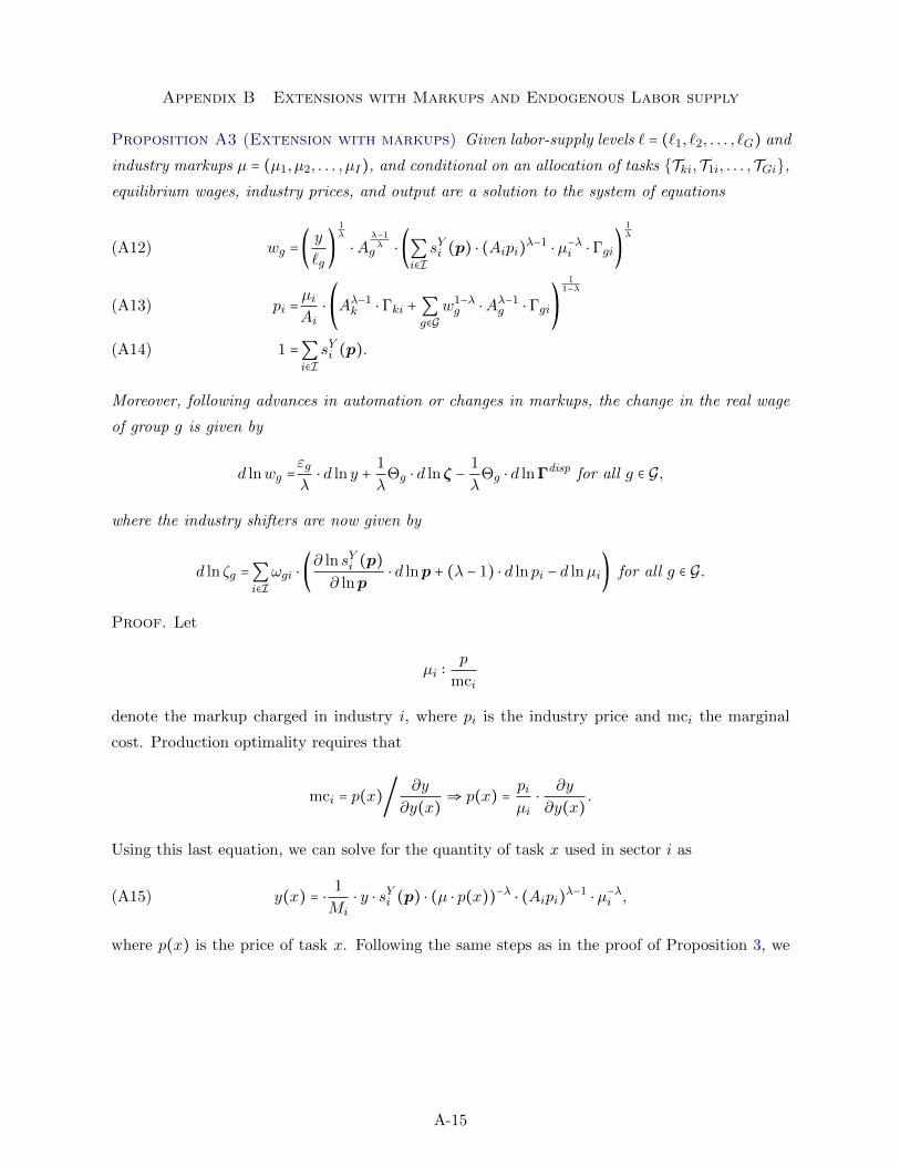
Appendix B Extensions with Markups and Endogenous Labor supply

Proposition A3 (Extension with markups) Given labor-supply levels ` = (`1, `2, . . . , `G) and

industry markups µ = (µ1, µ2, . . . , µI), and conditional on an allocation of tasks {Tki,T1i, . . . ,TGi},

equilibrium wages, industry prices, and output are a solution to the system of equations

wg =(y

`g)

1λ

⋅Aλ−1λg ⋅ (∑

i∈I

sYi (p) ⋅ (Aipi)λ−1

⋅ µ−λi ⋅ Γgi)

1λ

(A12)

pi =µiAi

⋅⎛

⎝Aλ−1k ⋅ Γki +∑

g∈G

w1−λg ⋅Aλ−1

g ⋅ Γgi⎞

⎠

11−λ

(A13)

1 =∑i∈I

sYi (p).(A14)

Moreover, following advances in automation or changes in markups, the change in the real wage

of group g is given by

d lnwg =εg

λ⋅ d ln y +

1

λΘg ⋅ d lnζ −

1

λΘg ⋅ d lnΓdisp for all g ∈ G,

where the industry shifters are now given by

d ln ζg =∑i∈I

ωgi ⋅ (∂ ln sYi (p)

∂ lnp⋅ d lnp + (λ − 1) ⋅ d lnpi − d lnµi) for all g ∈ G.

Proof. Let

µi ∶p

mci

denote the markup charged in industry i, where pi is the industry price and mci the marginal

cost. Production optimality requires that

mci = p(x)/∂y

∂y(x)⇒ p(x) =

piµi

⋅∂y

∂y(x).

Using this last equation, we can solve for the quantity of task x used in sector i as

y(x) = ⋅1

Mi⋅ y ⋅ sYi (p) ⋅ (µ ⋅ p(x))−λ ⋅ (Aipi)

λ−1⋅ µ−λi ,(A15)

where p(x) is the price of task x. Following the same steps as in the proof of Proposition 3, we

A-15

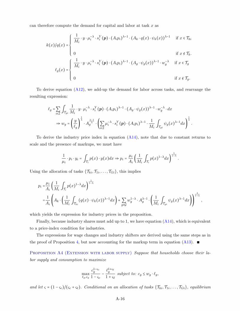
can therefore compute the demand for capital and labor at task x as

k(x)/q(x) =

⎧⎪⎪⎪⎪⎪⎪⎨⎪⎪⎪⎪⎪⎪⎩

1

Mi⋅ y ⋅ µ−λi ⋅ sYi (p) ⋅ (Aipi)

λ−1⋅ (Ak ⋅ q(x) ⋅ ψk(x))

λ−1 if x ∈ Tki

0 if x ∉ Tk.

`g(x) =

⎧⎪⎪⎪⎪⎪⎪⎨⎪⎪⎪⎪⎪⎪⎩

1

Mi⋅ y ⋅ µ−λi ⋅ sYi (p) ⋅ (Aipi)

λ−1⋅ (Ag ⋅ ψg(x))

λ−1⋅w−λ

g if x ∈ Tg

0 if x ∉ Tg.

To derive equation (A12), we add-up the demand for labor across tasks, and rearrange the

resulting expression:

`g =∑i∈I∫Tgi

1

Mi⋅ y ⋅ µ−λi ⋅ sYi (p) ⋅ (Aipi)

λ−1⋅ (Ag ⋅ ψg(x))

λ−1⋅w−λ

g ⋅ dx

⇒ wg = (y

`g)

1λ

⋅Aλ−1λg ⋅ (∑

i∈I

µ−λi ⋅ sYi (p) ⋅ (Aipi)λ−1

⋅1

Mi∫Tgi

ψg(x)λ−1dx)

1λ

.

To derive the industry price index in equation (A14), note that due to constant returns to

scale and the presence of markups, we must have

1

µi⋅ pi ⋅ yi = ∫

Ti

p(x) ⋅ y(x)dx⇒ pi =µiAi

(1

Mi∫Ti

p(x)1−λdx)

11−λ

.

Using the allocation of tasks {Tki,T1i, . . . ,TGi}, this implies

pi =µiAi

(1

Mi∫Ti

p(x)1−λdx)

11−λ

=1

Ai

⎛

⎝Ak ⋅ (

1

Mi∫Tki

(q(x) ⋅ ψk(x))λ−1dx) +∑

g∈G

w1−λg ⋅Aλ−1

g ⋅ (1

Mi∫Tgi

ψg(x)λ−1dx)

⎞

⎠

11−λ

,

which yields the expression for industry prices in the proposition.

Finally, because industry shares must add up to 1, we have equation (A14), which is equivalent

to a price-index condition for industries.

The expressions for wage changes and industry shifters are derived using the same steps as in

the proof of Proposition 4, but now accounting for the markup term in equation (A13).

Proposition A4 (Extension with labor supply) Suppose that households choose their la-

bor supply and consumption to maximize

max`g ,cg

c1−ςcg

1 − ςc−`1+ς`g

1 + ς`subject to: cg ≤ wg ⋅ `g,

and let ς = (1 − ςc)/(ςc + ς`). Conditional on an allocation of tasks {Tki,T1i, . . . ,TGi}, equilibrium

A-16

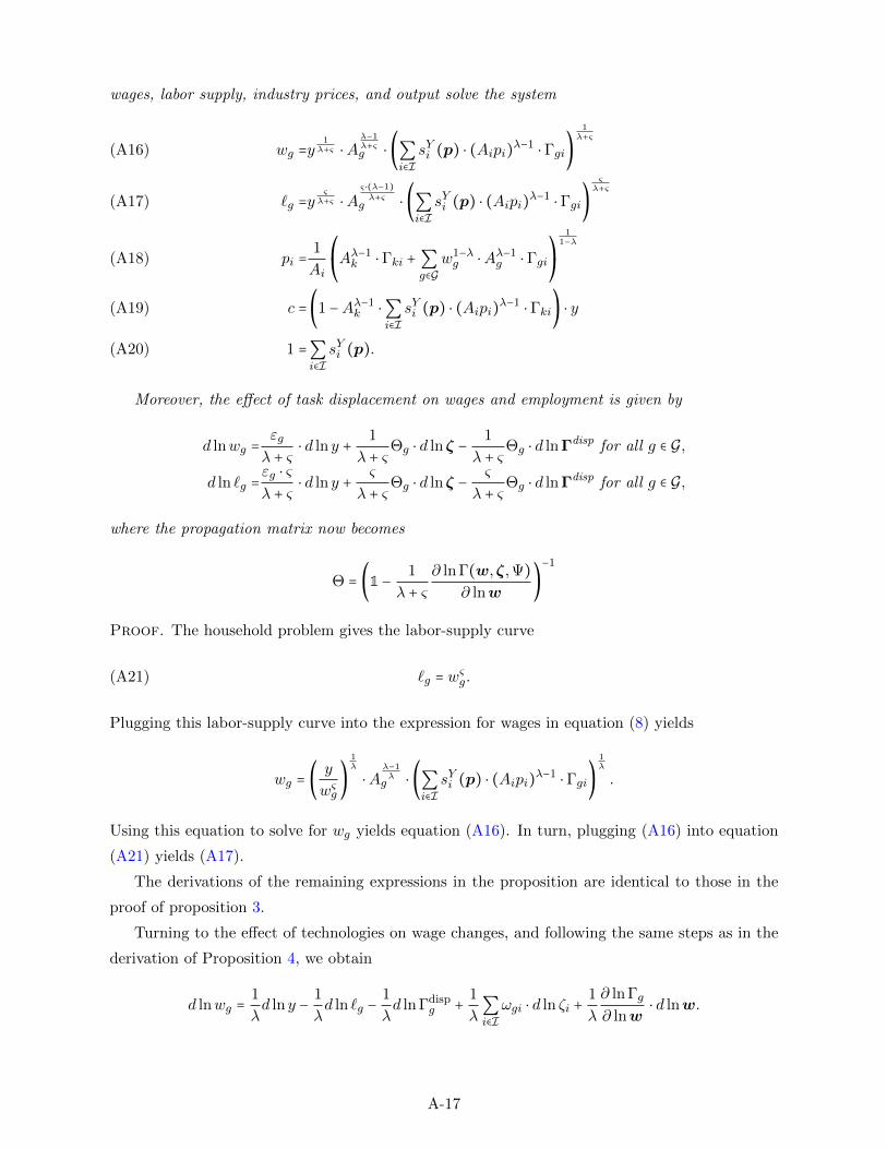
wages, labor supply, industry prices, and output solve the system

wg =y1λ+ς ⋅A

λ−1λ+ςg ⋅ (∑

i∈I

sYi (p) ⋅ (Aipi)λ−1

⋅ Γgi)

1λ+ς

(A16)

`g =yςλ+ς ⋅A

ς⋅(λ−1)λ+ς

g ⋅ (∑i∈I

sYi (p) ⋅ (Aipi)λ−1

⋅ Γgi)

ςλ+ς

(A17)

pi =1

Ai

⎛

⎝Aλ−1k ⋅ Γki +∑

g∈G

w1−λg ⋅Aλ−1

g ⋅ Γgi⎞

⎠

11−λ

(A18)

c =(1 −Aλ−1k ⋅∑

i∈I

sYi (p) ⋅ (Aipi)λ−1

⋅ Γki) ⋅ y(A19)

1 =∑i∈I

sYi (p).(A20)

Moreover, the effect of task displacement on wages and employment is given by

d lnwg =εg

λ + ς⋅ d ln y +

1

λ + ςΘg ⋅ d lnζ −

1

λ + ςΘg ⋅ d lnΓdisp for all g ∈ G,

d ln `g =εg ⋅ ς

λ + ς⋅ d ln y +

ς

λ + ςΘg ⋅ d lnζ −

ς

λ + ςΘg ⋅ d lnΓdisp for all g ∈ G,

where the propagation matrix now becomes

Θ = (1 −1

λ + ς

∂ ln Γ(w,ζ,Ψ)

∂ lnw)

−1

Proof. The household problem gives the labor-supply curve

`g = wςg.(A21)

Plugging this labor-supply curve into the expression for wages in equation (8) yields

wg = (y

wςg)

1λ

⋅Aλ−1λg ⋅ (∑

i∈I

sYi (p) ⋅ (Aipi)λ−1

⋅ Γgi)

1λ

.

Using this equation to solve for wg yields equation (A16). In turn, plugging (A16) into equation

(A21) yields (A17).

The derivations of the remaining expressions in the proposition are identical to those in the

proof of proposition 3.

Turning to the effect of technologies on wage changes, and following the same steps as in the

derivation of Proposition 4, we obtain

d lnwg =1

λd ln y −

1

λd ln `g −

1

λd ln Γdisp

g +1

λ∑i∈I

ωgi ⋅ d ln ζi +1

λ

∂ ln Γg

∂ lnw⋅ d lnw.

A-17

Using the fact that d ln `g = ς ⋅d lnwg (from the labor-supply curve in A21), we can rewrite this as

d lnwg =1

λ + ςd ln y −

1

λ + ςd ln Γdisp

g +1

λ + ς∑i∈I

ωgi ⋅ d ln ζi +1

λ + ς

∂ ln Γg

∂ lnw⋅ d lnw.

Solving this system for wage changes gives the formula for the propagation matrix in the propo-

sition.

A-18

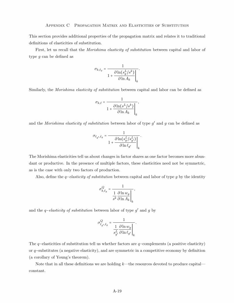
Appendix C Propagation Matrix and Elasticities of Substitution

This section provides additional properties of the propagation matrix and relates it to traditional

definitions of elasticities of substitution.

First, let us recall that the Morishima elasticity of substitution between capital and labor of

type g can be defined as

σk,`g =1

1 +∂ ln(sLg /s

k)

∂ lnAk

RRRRRRRRRRRk

.

Similarly, the Morishima elasticity of substitution between capital and labor can be defined as

σk,` =1

1 +∂ ln(sL/sk)

∂ lnAk

RRRRRRRRRRRk

,

and the Morishima elasticity of substitution between labor of type g′ and g can be defined as

σ`g′ ,`g =1

1 +∂ ln(sLg /s

Lg′)

∂ ln `g′

RRRRRRRRRRRk

.

The Morishima elasticities tell us about changes in factor shares as one factor becomes more abun-

dant or productive. In the presence of multiple factors, these elasticities need not be symmetric,

as is the case with only two factors of production.

Also, define the q−elasticity of substitution between capital and labor of type g by the identity

σQk,`g =1

1

sk∂ lnwg

∂ lnAk

RRRRRRRRRRRk

,

and the q−elasticity of substitution between labor of type g′ and g by

σQ`g′ ,`g=

1

1

sLg′

∂ lnwg

∂ ln `g′

RRRRRRRRRRRk

.

The q−elasticities of substitution tell us whether factors are q−complements (a positive elasticity)

or q−substitutes (a negative elasticity), and are symmetric in a competitive economy by definition

(a corollary of Young’s theorem).

Note that in all these definitions we are holding k—the resources devoted to produce capital—

constant.

A-19

Proposition A5 (Elasticities of substitution and Θ) The Morishima elasticity of substi-

tution between capital and labor is

σk,` =1

ε

λ+

1

sk⋅ (ε − 1)

where: ε ∶= ∑g∈G

sLg

sLεg ∈ (0,1).

Moreover, the Morishima elasticities of substitution between pairs of factors are

σk,`g =1

εg

λsk +

ε

λsL + (εg − 1) +

sL

sk(ε − 1)

σ`g′ ,`g =1

1 +sLg′

λ⋅⎛

⎝εg − εg′ −

⎛

⎝

θgg′

sLg′−θg′g′

sLg′

⎞

⎠

⎞

⎠

,

and the q−elasticities of substitution are

σQk,`g =1

εg

λ+

1

sk⋅ (εg − 1)

σQ`g′ ,`g=

1

1

λ⋅⎛

⎝εg −

θgg′

sLg′

⎞

⎠

.

Proof. First, note that we can rewrite the definition of the set Tg as

Tg ={x ∶1

ψg(x)⋅wg ⋅Ak

Ag≤

1

ψg′(x)⋅wg′ ⋅Ak

Ag′,

1

ψk(x) ⋅ q(x)∀g′}

Tk ={x ∶1

ψk(x) ⋅ q(x)≤

1

ψg′(x)⋅wg′ ⋅Ak

Ag′∀g′} .

These expressions imply that the effect of an increase in Ak on the allocation of tasks is

equivalent to a uniform rise in wages. That is:

∂ ln Γg

∂ lnAk=∑g′

∂ ln Γg

∂ lnwg′.

Using this property, we can compute the change in wages as

d lnwg =1

λd ln y +

1

λ

∂ ln Γg

∂ lnw⋅ d lnw +

1

λ

∂ ln Γg

∂ lnw⋅ d lnAk.

We can then solve for the change in wages as

d lnw =1

λΘd ln y +Θ

1

λΣ ⋅ d lnAk.

Moreover, using the definition of Θ, we get

Θ1

λΣ = Θ − 1.

A-20

Plugging this into the expression for wages, we obtain

d lnwg =εg

λ⋅ d ln y + (εg − 1)d lnAk.

Finally, holding k constant, we have that d ln y = sK ⋅ d lnAk. Therefore

1

σQk,`g

=1

sk∂ lnwg

∂ lnAk

RRRRRRRRRRRk

=εg

λ+

1

sk⋅ (εg − 1).(A22)

In addition, we also have that

∂ ln sLg

∂ lnAk

RRRRRRRRRRRk

= (εg

λ− 1) ⋅ sk + (εg − 1)(A23)

Using equation (A23), we can compute the Morishima elasticity of substitution between capital

and labor as

1

σk,`=1 +

∂ ln(sL/sk)

∂ lnAk

RRRRRRRRRRRk

=1 +1

sk⋅∂ ln sL

∂ lnAk

RRRRRRRRRRRk

=1 +1

sk∑g∈G

sLg

sL∂ ln sLg

∂ lnAk

RRRRRRRRRRRk

=1 +1

sk∑g∈G

sLg

sL⋅ ((

εg

λ− 1) ⋅ sk + (εg − 1))

=1 +1

sk((ε

λ− 1) ⋅ sk + (ε − 1))

=ε

λ+

1

sk⋅ (ε − 1)

Similarly, using equation (A23), we can compute the Morishima elasticity of substitution

between capital and labor of type g as

1

σk,`g=1 +

∂ ln(sLg /sk)

∂ lnAk

RRRRRRRRRRRk

=1 +∂ ln sLg

∂ lnAk

RRRRRRRRRRRk

+sL

sk∂ ln sL

∂ lnAk

RRRRRRRRRRRk

=1 + (εg

λ− 1) ⋅ sk + (εg − 1) +

sL

sk((ε

λ− 1) ⋅ sk + (ε − 1))

=εg

λsk +

ε

λsL + (εg − 1) +

sL

sk(ε − 1).

A-21

We now turn to the elasticities involving chnages in `g′ . Following a change in `g′ , we have:

d lnwg =εg

λd ln y −

θgg′

λd ln `g′ .(A24)

Holding k constant, d ln y = sLg′ ⋅ d ln `g′ . Therefore,

1

σQ`g′ ,`g

=1

sLg′

∂ lnwg

∂ ln `g′

RRRRRRRRRRRk

=1

λ⋅⎛

⎝εg −

θgg′

sLg′

⎞

⎠.

Finally, we can write the Morishima elasticity of substitution between labor of type g′ and g

as

1

σ`g′ ,`g= 1 +

∂ ln(sLg /sLg′)

∂ ln `g′

RRRRRRRRRRRk

= 1 +∂ lnwg

∂ ln `g′

RRRRRRRRRRRk

−∂ lnwg′

∂ ln `g′

RRRRRRRRRRRk

.

Using the formula for the change in wages in equation (A24), we obtain

1

σ`g′ ,`g= 1 +

sLg′

λ⋅⎛

⎝εg − εg′ −

⎛

⎝

θgg′

sLg′−θg′g′

sLg′

⎞

⎠

⎞

⎠,

which completes proof of the proposition.

Proposition A6 (Quasi-symmetry of the propagation matrix) The propagation matrix

satisfies the symmetry property

εg −θgg′

sLg′= εg′ −

θg′g

sLg.(A25)

Proof. By definition σQ`g′ ,`g= σQ`g ,`g′

, which implies the symmetry property in (A25).

A-22

Appendix D Estimating the Propagation Matrix

This appendix provides additional details regarding the estimation of the propagation matrix. It

also describes an alternative parametrization.

Common diagonal θgg = θ

Our baseline estimation strategy makes two assumptions:

• The propagation matrix has a common diagonal term θgg = θ ≥ 0. This is motivated by the

strong reduced form evidence between task displacement and the observed change in real

wages.

• The extent of competition for tasks between groups is determined by their similarity across

a set of characteristics N . We operationalize this by assuming that

θgg′

sLg′+θg′g

sLg= 2 ∑

n∈N

βn ⋅ f(dng,g′).

Using these two assumptions, and combining them with the theoretical restriction that

εg −θgg′

sLg′= εg′ −

θg′g

sLg,

yields the parametrization used in the main text.

Common elasticities εg

Our baseline estimates allow εg to vary across groups but fixes θgg to a common value. We now

outline an estimation approach based on the alternative assumption that

∑g′θgg′ = εg = ε for all g,

which implies that all wages rise by the same amount in response to a factor-neutral increase in

output.

With this assumption, the symmetry property derived in Proposition A6 becomes:

θgg′

sLg′=θg′g

sLg,

which motivates a parametrization where the extent of competition between g′ and g depends on

A-23

how similar these groups are along several characteristics n ∈ N . In particular, we assume

θgg′ = ∑n∈N

βn ⋅ f(dng,g′) ⋅ s

Lg′ for all g′ ≠ g

θgg =ε − ∑g′≠g∑n∈N

βn ⋅ f(dng,g′) ⋅ s

Lg′ ,

where f is a decreasing function of the distance along a given dimension n between groups g′ and

g, denoted here by dng,g′ .

Thus, For a given set of characteristics n ∈ N , we estimate {βn}n∈N and ε using the equation

d lnwg =ε ⋅ d ln y − ε ⋅Task displacementg(A26)

− ∑n∈N

βn ⋅ ∑g′≠g

f(dng,g′) ⋅ sLg′ ⋅ (Task displacementg′ −Task displacementg) + υg,

imposing the restriction that βn ≥ 0.

Additional estimates and robustness

Besides the exercises summarized in the main text, we conducted several robustness checks re-

garding our estimation of the propagation matrix. In particular, Table A16 provides estimates

using a tuning parameter of κ = 1 and κ = 5 (recall that our baseline uses a quadratic decay with

κ = 2). This table also summarizes the results obtained using our alternative estimation approach,

described in the previous section, and assuming a common row sum εg = ε.

A-24

Appendix E Measuring Task Displacement

Theoretical derivations

This section derives our measures of task displacement in the extended version of our model that

allows for markups.

We assume that tasks can be partitioned into routine tasksRi and non-routine tasksNi, whose

union equals Ti. Moreover, let Rgi and Ngi denote the (disjoint) sets of routine and non-routine

tasks allocated to workers of type g.

Assumption 2 is equivalent to:

i Only routine tasks have been automated, which implies that Dgi ⊂Rgi

ii Routine tasks in a given industry have been automated at the same rate for all workers,

which implies that

∫Dgi ψg(x)λ−1dx

∫Rgi ψg(x)λ−1dx

= ϑi ≥ 0 for all g.

Before continuing with our derivations, we introduce some notation that we will use throughout

this appendix. Define by ωYX the share of wages in some cell X earned within another sub-cell

Y . For example, define ωig as the share of wages earned by members of group g in industry i as a

fraction of their total wage income:

ωig =sYi ( p) ⋅ (Aipi)

λ−1⋅ Γgi

∑g′sYg′( p) ⋅ (Ag′pg′)

λ−1⋅ Γgg′

.

Define ωRgi as the share of wages earned by members of group g in industry i in routine jobs as a

fraction of the total wage income earned by workers of group g in industry i:

ωRgi =∫Rgi

ψg(x)λ−1dx

∫Tgi

ψg(x)λ−1dx

.

And define ωRi as the share of wages earned by workers in industry i in routine jobs as a fraction

of the total wage income earned by workers in industry i:

ωRi =

∑g∈G

w1−λg ∫

Rgi

ψg(x)λ−1dx

∑g∈G

w1−λg ∫

Tgi

ψg(x)λ−1dx

.

A-25

We next define the average cost-saving gains from automating tasks in sector i as

πi = ∑g∈G

ωRgiωRi

⋅ πgi,

where ωRgi is the share of wages in industry i paid to g workers in routine jobs, and ωRi is the

share of wages in industry i paid to workers in routine jobs.

Finally, for each type of worker g, define the elasticity σLgi by

1

ωgi⋅∂ ln sLi∂ lnwg

= sk ⋅ (1 − σLgi).

When σLgi > 1, an increase in wg reduces the labor share. Instead, when σLgi < 1, an increase in wg

increases the labor share.

The following proposition characterizes the change in the labor share as a function of various

driving forces:

1. task displacement generated by automation or offshoring, d ln Γdispgi generating productivity

gains πgi > 0;

2. productivity deepening and factor augmenting technologies taking place in that industry,

and denoted by d ln Γdeeppgi and d lnAgi. Note that, in this proposition, factor-augmenting

technologies may vary by industry;

3. changes in markups at the industry level, denoted by d lnµi;

4. changes in wages, d lnwg due to other shocks in the economy or changes in factor supplies;

5. and changes in the user cost of capital. In particular, we assume there are two types of

technologies increasing the productivity of capital or reducing its price. On the one hand

we have the task displacement technologies introduced above. And on the other hand, we

have uniform declines in the user cost of capital driven by lower capital prices at all tasks

or cheap access to credit. Formally, we write q(x) = 1Ri

⋅ q0(x) and consider changes in

q0(x) leading to task displacement or changes in Ri common to all uses of capital in a given

industry.

Proposition A7 (Industry labor shares) Let sLi denote the labor share in industry i. Also,

let q(x) = 1Ri

⋅ q0(x), where Ri captures uniform changes in the price of capital at all tasks in

industry i, and let wegi = wg/Agi denote the wages per efficiency unit of labor paid in industry i for

workers of type g. Following a change in technology (task displacement, productivity deepening,

A-26

Aki, Agi, and Ai) factor prices (wg, Ri), and markups µi, we have

d ln sLi = − d lnµi − (1 + (λ − 1) ⋅ sLi ⋅ πi) ⋅ ωRi ⋅ ϑi

+ (1 − sLi ) ⋅ (λ − 1) ⋅⎛

⎝∑g∈G

ωgi ⋅ d ln Γdeepgi − d ln Γdeep

ki

⎞

⎠

+ (1 − sLi ) ⋅ (1 − σLi ) ⋅ d lnwei − (1 − sLi ) ⋅ (1 − σ

Ki ) ⋅ d ln(Ri/Aki),

where

σLi ∶=∑g∈G

ωgi ⋅ d lnweg

∑g′ ωg′

i ⋅ d lnweg′⋅ σLgi σKi ∶=∑

g∈G

ωgi ⋅ σLgi,

and

d lnwei = ∑g∈G

ωgi ⋅ d lnwegi.

Proof. Given a vector of wages and technologies, we can write the labor share as

sLi =1

µi⋅

∑g∈G

wegi1−λ

⋅ Γgi

Aλ−1k ⋅ Γki +∑

g∈G

wegi1−λ

⋅ Γgi,(A27)

where recall that the denominator is also equal to

p1−λi = Aλ−1

k ⋅ Γki +∑g∈G

wegi1−λ

⋅ Γgi.

We can decompose changes in the labor share into four terms:

d ln sLi =contribution of

markups+

contribution of

task displacement+

contribution of

prod. deepening

+contribution of

eff. wage changes+

contribution of

price of capital,

which we now derive in detail.

1. Contribution of markups: this is simply given by −d lnµi.

2. Contribution of task displacement: we can compute this as

contribution of

task displacement= −∑

g∈G

ωRgi ⋅ ϑi + (1 − λ) ⋅ sLi ⋅∑g∈G

ωRgi ⋅ ϑi ⋅ πgi

where the first term captures the effect of task displacement on the numerator and the second

term the effect on the denominator of the labor share expression in equation (A27). Using the

A-27

definition of πi, this can be simplified as

contribution of

task displacement= − (1 + (λ − 1) ⋅ sLi ⋅ πi) ⋅ ω

Ri ⋅ ϑi.

3. Contribution of productivity deepening: we can compute this as

contribution of

prod. deepening= (λ − 1) ⋅∑

g∈G

ωgi ⋅ d ln Γdeepgi − (λ − 1) ⋅

⎛

⎝sLg ⋅∑

g∈G

ωgi ⋅ d ln Γdeepgi + ski ⋅ d ln Γdeep

ki

⎞

⎠,

where the first term captures the effect of task displacement on the numerator and the second

term the effect on the denominator of the labor share expression in equation (A27). We can

rewrite this as

contribution of

prod. deepening= (λ − 1) ⋅ (1 − sLi ) ⋅

⎛

⎝∑g∈G

ωgi ⋅ d ln Γdeepgi − d ln Γdeep

ki

⎞

⎠

4. Contribution of wages per efficiency unit of labor: We now turn to the contribution of

wages per efficiency unit of labor. Using the definition of σLgi, we can compute their effect as

contribution of

wage changes= ∑g∈G

ωgi ⋅ (1 − sLi ) ⋅ (1 − σ

Lgi) ⋅ d lnwegi.

Using the definition of σLi and d lnwi, we obtain

contribution of

wage changes= (1 − sLi ) ⋅ (1 − σ

Li ) ⋅ d lnwi.

5. Contribution of price of capital: To compute the effects of a uniform change in capital

prices, we first provide explicit formulas for σLgi, which we will use in our derivations below. We

have that

1

ωgi⋅∂ ln sLi∂ lnwg

=1

ωgi⋅⎛

⎝ωgi ⋅ (1 − λ) +∑

g′ωg

′

i ⋅∂ ln Γg′i

∂ lnwg′i− sL ⋅ ωgi ⋅ (1 − λ)

⎞

⎠,

where the first two terms capture the effect of task displacement on the numerator and the third

term the effect on the denominator of the labor share expression in equation (A27). Here, we

used the fact that the effect of wages on the denominator equals the direct effect holding the task

allocation constant—an implication of the envelope theorem. We can rewrite this expression as

1

ωgi⋅∂ ln sLi∂ lnwg

= (1 − sLi ) ⋅ (1 − λ) +∑g′

ωg′

i

ωgi⋅∂ ln Γg′i

∂ lnwg′i,

A-28

which implies that

σLgi = λ −1

1 − sLi⋅∑g′

ωg′

i

ωgi⋅∂ ln Γg′i

∂ lnwg′i,

and

(1 − sLi ) ⋅ (λ − σLgi) =∑∑

g′

ωg′

i

ωgi⋅∂ ln Γg′i

∂ lnwg′i.(A28)

Consider a uniform change in the cost per efficiency unit of capital d ln(Ri/Aki) on the labor

share of industry i. The effect of this change in the allocation of tasks is the same as a uniform

reduction in wages of d ln(Ri/Aki). Moreover, the effect of d ln(Ri/Aki) on the denominator of

the labor share is just its direct effect—an application of the envelope theorem. Thus, we get

contribution of

price of capital= −∑

g∈G

∑g′ωg

′

i ⋅∂ ln Γg′i

∂ lnwg⋅ d ln(Ri/Aki) − s

ki ⋅ (1 − λ) ⋅ d ln(Ri/Aki),

where the first term captures the effect of task changes on the numerator and the second term

the effect on the denominator of the labor share expression in equation (A27). Using equation

(A28), we can rewrite this expression as

contribution of

price of capital= −∑

g∈G

ωgi ⋅ (1 − sLi ) ⋅ (λ − σ

Lgi) ⋅ d ln(Ri/Aki) − s

ki ⋅ (1 − λ) ⋅ d ln(Ri/Aki).

Finally, using the definition of σKi , we can rewrite this as

contribution of

price of capital= −(1 − sLi ) ⋅ (1 − σ

Ki ) ⋅ d ln(Ri/Aki),

which completes the proof of the proposition

We are now in a position to derive the measures of task displacement used in the text. We

start with the case with no ripple effects, no change in markups, and λ = 1, which gives the

baseline measure in equation (12).

Proposition A8 Suppose that Assumptions 1 and 2 hold. Suppose also that λ = 1 and there are

no markups. Then σLi = σKi = 1 and task displacement can be computed as

d ln Γdispg =∑

i∈I

ωig ⋅ωRgi

ωRi⋅ (−d ln sLi ) and d ln Γdisp

gi =ωRgi

ωRi⋅ (−d ln sLi ).

A-29

Moreover, total task displacement taking place in industry i is given by

d ln Γdispi =∑

i∈I

ωgi ⋅ d ln Γdispgi = (−d ln sLi ).

Proof. Proposition A7 implies that

d ln sLi = −ωRi ⋅ ϑi ⇒ ϑi =(−d ln sLi )

ωRi.

Moreover, by definition

d ln Γdispgi =

∫Dgi ψg(x)λ−1dx

∫Tgi ψg(x)λ−1dx

=∫Rgi ψg(x)

λ−1dx

∫Tgi ψg(x)λ−1dx

⋅∫Dgi ψg(x)

λ−1dx

∫Rgi ψg(x)λ−1dx

= ωRgi ⋅ ϑi =ωRgi

ωRi⋅ (−d ln sLi ).

and task displacement for worker groups is given by

d ln Γdispg =∑

i∈I

ωig ⋅ d ln Γdispgi =∑

i∈I

ωigωRgi

ωRi⋅ (−d ln sLi ).

The next Proposition derives the more general measure in footnote 15.

Proposition A9 Suppose that Assumptions 1 and 2 hold. Then, σLi = σKi = λ. In the ab-

sence of productivity deepening or factor-augmenting technologies affecting the labor share, task

displacement can be computed as

d ln Γdispg =∑

i∈I

ωig ⋅ωRgi

ωRi⋅−d ln sLi − d lnµi + (1 − sLi ) ⋅ (1 − λ) ⋅ (d lnwi − d lnRi)

1 + (λ − 1) ⋅ sLi ⋅ πi

d ln Γdispgi =

ωRgi

ωRi⋅−d ln sLi − d lnµi + (1 − sLi ) ⋅ (1 − λ) ⋅ (d lnwi − d lnRi)

1 + (λ − 1) ⋅ sLi ⋅ πi.

Moreover, total task displacement taking place in industry i is given by

d ln Γdispi =∑

i∈I

ωgi ⋅ d ln Γdispgi =

−d ln sLi − d lnµi + (1 − sLi ) ⋅ (1 − λ) ⋅ (d lnwi − d lnRi)

1 + (λ − 1) ⋅ sLi ⋅ πi.

Proof. Proposition A7 implies that

d ln sLi = −d lnµi − (1 + (λ − 1) ⋅ sLi ⋅ πi) ⋅ ωRi ⋅ ϑi + (1 − sLi ) ⋅ (1 − λ) ⋅ (d lnwi − d lnRi),

which gives

ϑi =−d ln sLi − d lnµi + (1 − sLi ) ⋅ (1 − λ) ⋅ (d lnwi − d ln qi)

(1 + (λ − 1) ⋅ sLi ⋅ πi) ⋅ ωRi

.

A-30

Moreover, following the same steps as in the proof of Proposition A8, we get

d ln Γdispgi =

∫Dgi ψg(x)λ−1dx

∫Tgi ψg(x)λ−1dx

=∫Rgi ψg(x)

λ−1dx

∫Tgi ψg(x)λ−1dx

⋅∫Dgi ψg(x)

λ−1dx

∫Rgi ψg(x)λ−1dx

= ωRgi ⋅ ϑi

=ωRgi

ωRi⋅−d ln sLi − d lnµi + (1 − sLi ) ⋅ (1 − λ) ⋅ (d lnwi − d lnRi)

1 + (λ − 1) ⋅ sLi ⋅ πi.

and task displacement for worker groups is given by

d ln Γdispg =∑

i∈I

ωig ⋅ d ln Γdispgi =∑

i∈I

ωig ⋅ωRgi

ωRi⋅−d ln sLi − d lnµi + (1 − sLi ) ⋅ (1 − λ) ⋅ (d lnwi − d lnRi)

1 + (λ − 1) ⋅ sLi ⋅ πi.

Our final Proposition derives a version of our measure of task displacement that allows for

ripple effects. Equation (16) corresponds to the special case of this formula when there are no

changes in markups and σLi = σKi .

Proposition A10 Suppose that Assumptions 2 holds. In the absence of productivity deepening

or factor-augmenting technologies affecting the labor share, task displacement can be computed as

d ln Γdispg =∑

i∈I

ωig ⋅ωRgi

ωRi⋅−d ln sLi − d lnµi + (1 − sLi ) ⋅ (1 − σ

Li ) ⋅ d lnwi − (1 − sLi ) ⋅ (1 − σ

Ki ) ⋅ d lnRi

1 + (λ − 1) ⋅ sLi ⋅ πi

d ln Γdispgi =

ωRgi

ωRi⋅−d ln sLi − d lnµi + (1 − sLi ) ⋅ (1 − σ

Li ) ⋅ d lnwi − (1 − sLi ) ⋅ (1 − σ

Ki ) ⋅ d lnRi

1 + (λ − 1) ⋅ sLi ⋅ πi.

Moreover, total task displacement taking place in industry i is given by

d ln Γdispi =∑

i∈I

ωgi ⋅ d ln Γdispgi =

−d ln sLi − d lnµi + (1 − sLi ) ⋅ (1 − σLi ) ⋅ d lnwi − (1 − sLi ) ⋅ (1 − σ

Ki ) ⋅ d lnRi

1 + (λ − 1) ⋅ sLi ⋅ πi.

Proof. Proposition A7 implies that

d ln sLi = −d lnµi − (1 + (λ − 1) ⋅ sLi ⋅ πi) ⋅ ωRi ⋅ ϑi + (1 − sLi ) ⋅ (1 − σ

Li ) ⋅ d lnwi − (1 − sLi ) ⋅ (1 − σ

Ki ) ⋅ d lnRi,

which gives

ϑi =−d ln sLi − d lnµi + (1 − sLi ) ⋅ (1 − σ

Li ) ⋅ d lnwi − (1 − sLi ) ⋅ (1 − σ

Ki ) ⋅ d lnRi

(1 + (λ − 1) ⋅ sLi ⋅ πi) ⋅ ωRi

.

A-31

Following the same steps as in the proof of Proposition A8, we get

d ln Γdispgi =

∫Dgi ψg(x)λ−1dx

∫Tgi ψg(x)λ−1dx

=∫Rgi ψg(x)

λ−1dx

∫Tgi ψg(x)λ−1dx

⋅∫Dgi ψg(x)

λ−1dx

∫Rgi ψg(x)λ−1dx

= ωRgi ⋅ ϑi

=ωRgi

ωRi⋅−d ln sLi − d lnµi + (1 − sLi ) ⋅ (1 − σ

Li ) ⋅ d lnwi − (1 − sLi ) ⋅ (1 − σ

Ki ) ⋅ d lnRi

1 + (λ − 1) ⋅ sLi ⋅ πi.

and task displacement for worker groups is given by

d ln Γdispg =∑

i∈I

ωig ⋅ d ln Γdispgi

=∑i∈I

ωig ⋅ωRgi

ωRi⋅−d ln sLi − d lnµi + (1 − sLi ) ⋅ (1 − σ

Li ) ⋅ d lnwi − (1 − sLi ) ⋅ (1 − σ

Ki ) ⋅ d lnRi

1 + (λ − 1) ⋅ sLi ⋅ πi.

Empirical implementation and bounding exercise

The empirical implementation of our measures of task displacement in Propositions A8 and A9 is

straightforward. However, the formulas in Proposition A10 depend on two elasticities of substi-

tution, σKi and σLi , which may differ due to the fact that we have different types of workers, and

that when wages rise in one industry, we may be capturing the substitution of different worker

groups for capital in marginal tasks. When implementing these formulas, we will assume that

σKi = σLi , and use empirical estimates of the elasticity of substitution between capital and labor

at the industry level, σi, to discipline their common value. This is motivated by the fact that

empirical estimates of the elasticity of substitution between capital and labor are also estimating

some combination of the group-specific elasticities, σLgi’s.

In addition, when computing task displacement, we will use empirical estimates of d lnwi and

d lnRi from the BLS, which account for changes in wages, the quality of workers, and quality-

adjusted prices of capital used in an industry. We note also that, although our model has common

wages for a given skill across industries, the expressions in Propositions A9 and A10 apply with-

out modification to the case in which wages are industry-specific. In addition, our formula is

not affected by factor-neutral improvements in TFP in industry i, since these do not affect an

industry’s labor share.

While our formulas incorporate the effects of changes in factor prices, they miss the contribu-

tion of general factor-augmenting technologies. Now we provide upper bounds on the effects of

this type of technological change on our estimates of task displacement, which will reveal that this

type of technological change tends to have a very small effect on our inferred task displacement

A-32

measure.

We focus on our measures in Proposition A10 obtained for λ = 0.5 and σi ranging from 0.8 to 1.2

(these technologies do not affect our measures if σi = 1). In particular, for σi < 1, the contribution

of factor-augmenting technologies to the change in the labor share is between −sKi ⋅(1−σi) ⋅d lnA`i

(where d lnA`i is a weighted average of d lnAgi across workers) and sKi ⋅(1−σi) ⋅d lnAki. Moreover,

assuming no technological regress, we have that the total increase in (gross output) TFP in

industry i must exceed both sLi ⋅ d lnALi and sKi ⋅ d lnAki, where now sLi and sKi denote the share

of labor and capital in gross output (an application of Hulten’s theorem). As a result, we can

bound the contribution of factor-augmenting technologies to lie in the interval

[−sKisLi

⋅ (1 − σi) ⋅ d ln TFPi,sKisKi

⋅ (1 − σi) ⋅ d ln TFPi] .

Likewise, for σi > 1, the contribution of factor-augmenting technologies to the change in the labor

share is between −sKi ⋅ (σi − 1) ⋅ d lnAki and sKi ⋅ (σi − 1) ⋅ d lnA`i, which we can bound by

[−sKisKi

⋅ (σi − 1) ⋅ d ln TFPi,sKisLi

⋅ (σi − 1) ⋅ d ln TFPi] .

Figure A4 presents our measures of task displacement across industries and worker groups

using equation (16) for σi = 0.8 and for σi = 1.2, depicting the bounds on the contribution of

factor-augmenting technologies using the whiskers. When constructing these bounds, we assume

that industries with declining TFP between 1987 and 2016, experienced no factor-augmenting

improvements. Except for a handful of IT-intensive industries with vast increases in TFP (elec-

tronics, computers, and communications), our bounds exclude anything other than very small

effects of factor-augmenting technologies on the decline in labor shares and our task displacement

measure. This is because these technologies have limited distributional effects but generate large

TFP gains. Through the lens of our model, and given the pervasive lack of productivity growth

observed across industries, these technologies cannot play a key role in explaining the decline in

the labor share.

A-33

Appendix F Data Appendix

Industry data: Our main source of industry-level data are the BEA Integrated industry ac-

counts for 1987–2016. These data contain information on industry value added, labor compensa-

tion, industry prices and factor prices for 61 NAICS industries. We aggregated these data to the

49 industries used in our analysis, which we could track consistently both in the BEA and the

worker-level data from the 1980 US Census. Finally, when computing changes in industry’s labor

shares, we winsorized labor shares in value added at 20% to reduce noise in our measures of task

displacement coming from industries with low and volatile labor shares.

Besides the BEA data, we also used data from the BLS multifactor productivity tables for

1987–2016. These data are also available for 61 NAICS industries which we aggregated to the 49

industries used in our analysis.

We complement the industry data with proxies for the adoption of automation technologies

across industries. First, we use the measure of adjusted penetration of robots from Acemoglu and

Restrepo (2020), which is available for 1993–2014. These measure is constructed using data from

the International Federation of Robotics, and is defined for each industry i as

APRi =1

5

5

∑e=1

[robotse,i,2014 − robotse,i,1993

`e,i,1993− output growthe,i,2004−1993 ⋅

robotse,i,1993

`e,i,1993] ,

where the right-hand side is computed as an average among five European countries, e, leading

the US in the adoption of industrial robots (see Acemoglu and Restrepo, 2020, for details). These

measure is available for all of our manufacturing industries, but has a coarser resolution outside

of manufacturing.

Finally, we also use the share of software and specialized machinery in value added from the

BLS multifactor productivity tables. In particular, we use the detailed capital tables from the

BLS, which provide the compensation for different assets (computed as the user cost of each asset

multiplied by its stock). For software, we add custom-made software or software developed in

house—which are more relevant for automation than pre-packaged software like Stata or Word.

For specialized machinery, we add metalworking machinery (typically numerically controlled ma-

chines capable of automatically producing a pre-specified task), agricultural machinery other than

tractors, specialized machinery used in the service sector, specialized machinery used in industry

applications (which should also include industrial robots), construction machinery, and material

handling equipment used in industrial applications. Although not all software and dedicated

machinery necessarily involve the automation of tasks previously performed by labor, the com-

ponent of these measures associated with significant declines in the labor share helps isolate the

automation component.

For offshoring, we use a measure from Feenstra and Hanson (1999) recently updated by Wright

(2014) for 1990–2007. This measure captures changes in the share of imported intermediates across

industries, and is only available for the manufacturing sector. When using it, we set it to zero

A-34

outside of manufacturing.

When using these proxies of automation and offshoring, we rescale the coefficients on our

reduced-form estimates by the first-stage relationship between each of these variables and task

displacement at the industry level reported in Panel B of Table A1.

Turning to our proxies for changes in market structure, we use changes in sales concentration

and several estimates of markups aggregated at the industry level. Our data for sales concentration

comes from the Census Statistics of U.S. Businesses (SUSB) and is only available for 1997–2016.

Using these data, we computed the tail index of the sales distribution for all the industries in our

sample. The SUSB data can also be used to compute tail indices for the employment distribution

going back to 1992. Using this alternative proxy of concentration available over a longer period

didn’t alter our findings.

For markups, we provide three different estimates.

First, we compute markups in a given industry using an accounting approach, which measures

markups by the ratio of output to costs:

µi =gross outputi

RiKi +Variable inputsi.

This approach requires constant returns to scale and assumes there are no adjustment costs.

This approach also requires a measurement of the unobserved user cost of capital Ri. We follow

Karabarbounis and Neiman (2018) and compute Ri using a user-cost formula accounting for

changes in taxes. We do this using data on capital stocks and prices from NIPA’s Fixed Asset

Tables. We also set the internal rate of return to 6% and keep it constant over time. As shown

in Karabarbounis and Neiman (2013), the alternative approach of using bond rates to proxy for

firms’ and investors’ internal rates of return yields large, volatile, and unreasonable estimates of

aggregate markups. More relevant for our exercise is the fact that different values of the internal

rate of return do not affect the variation in relative trends in markups across industries.

Second, we compute the change in markups by looking at the percent decline in the share of

materials in gross output. That is:

∆ lnµi = −∆ ln share materialsi.

This approach assumes that the share of materials in total costs is constant, and that a decline

in the share of materials thus reveals higher markups. We use the BEA data described above

to measure the share of materials in gross output. Outside of manufacturing, we focus on the

share of materials and intermediate services, since raw materials play a smaller role in the service

sector.

Finally, we compute markups using a production function approach as in De Loecker, Eeckhout

A-35

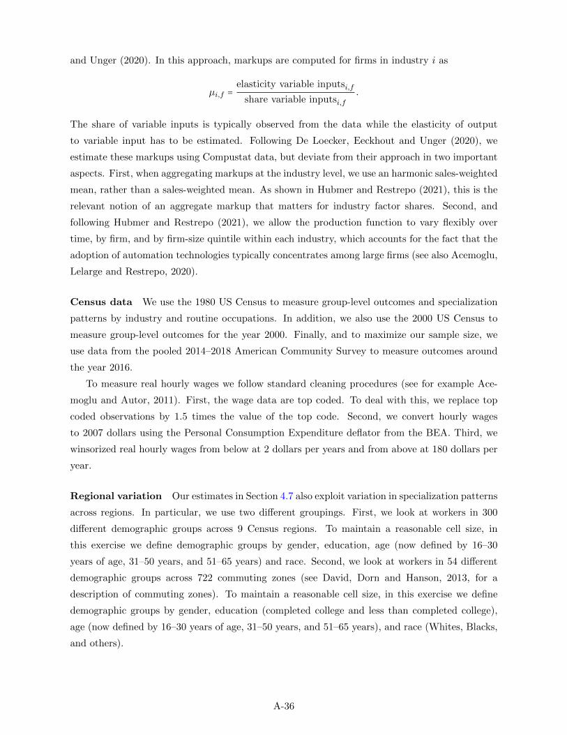
and Unger (2020). In this approach, markups are computed for firms in industry i as

µi,f =elasticity variable inputsi,f

share variable inputsi,f.

The share of variable inputs is typically observed from the data while the elasticity of output

to variable input has to be estimated. Following De Loecker, Eeckhout and Unger (2020), we

estimate these markups using Compustat data, but deviate from their approach in two important

aspects. First, when aggregating markups at the industry level, we use an harmonic sales-weighted

mean, rather than a sales-weighted mean. As shown in Hubmer and Restrepo (2021), this is the

relevant notion of an aggregate markup that matters for industry factor shares. Second, and

following Hubmer and Restrepo (2021), we allow the production function to vary flexibly over

time, by firm, and by firm-size quintile within each industry, which accounts for the fact that the

adoption of automation technologies typically concentrates among large firms (see also Acemoglu,

Lelarge and Restrepo, 2020).

Census data We use the 1980 US Census to measure group-level outcomes and specialization

patterns by industry and routine occupations. In addition, we also use the 2000 US Census to

measure group-level outcomes for the year 2000. Finally, and to maximize our sample size, we

use data from the pooled 2014–2018 American Community Survey to measure outcomes around

the year 2016.

To measure real hourly wages we follow standard cleaning procedures (see for example Ace-

moglu and Autor, 2011). First, the wage data are top coded. To deal with this, we replace top

coded observations by 1.5 times the value of the top code. Second, we convert hourly wages

to 2007 dollars using the Personal Consumption Expenditure deflator from the BEA. Third, we

winsorized real hourly wages from below at 2 dollars per years and from above at 180 dollars per

year.

Regional variation Our estimates in Section 4.7 also exploit variation in specialization patterns

across regions. In particular, we use two different groupings. First, we look at workers in 300

different demographic groups across 9 Census regions. To maintain a reasonable cell size, in

this exercise we define demographic groups by gender, education, age (now defined by 16–30

years of age, 31–50 years, and 51–65 years) and race. Second, we look at workers in 54 different

demographic groups across 722 commuting zones (see David, Dorn and Hanson, 2013, for a

description of commuting zones). To maintain a reasonable cell size, in this exercise we define

demographic groups by gender, education (completed college and less than completed college),

age (now defined by 16–30 years of age, 31–50 years, and 51–65 years), and race (Whites, Blacks,

and others).

A-36

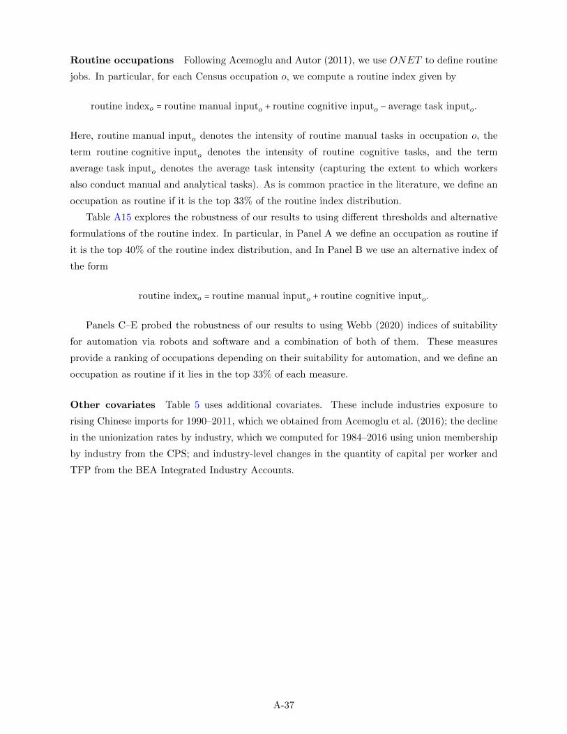
Routine occupations Following Acemoglu and Autor (2011), we use ONET to define routine

jobs. In particular, for each Census occupation o, we compute a routine index given by

routine indexo = routine manual inputo + routine cognitive inputo − average task inputo.

Here, routine manual inputo denotes the intensity of routine manual tasks in occupation o, the

term routine cognitive inputo denotes the intensity of routine cognitive tasks, and the term

average task inputo denotes the average task intensity (capturing the extent to which workers

also conduct manual and analytical tasks). As is common practice in the literature, we define an

occupation as routine if it is the top 33% of the routine index distribution.

Table A15 explores the robustness of our results to using different thresholds and alternative

formulations of the routine index. In particular, in Panel A we define an occupation as routine if

it is the top 40% of the routine index distribution, and In Panel B we use an alternative index of

the form

routine indexo = routine manual inputo + routine cognitive inputo.

Panels C–E probed the robustness of our results to using Webb (2020) indices of suitability

for automation via robots and software and a combination of both of them. These measures

provide a ranking of occupations depending on their suitability for automation, and we define an

occupation as routine if it lies in the top 33% of each measure.

Other covariates Table 5 uses additional covariates. These include industries exposure to

rising Chinese imports for 1990–2011, which we obtained from Acemoglu et al. (2016); the decline

in the unionization rates by industry, which we computed for 1984–2016 using union membership

by industry from the CPS; and industry-level changes in the quantity of capital per worker and

TFP from the BEA Integrated Industry Accounts.

A-37

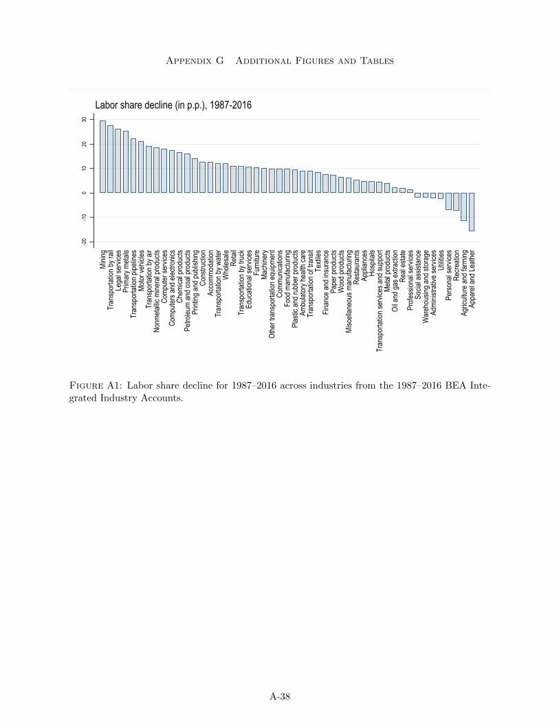
Appendix G Additional Figures and Tables

-20

-10

010

2030

Minin

gTr

ansp

ortat

ion by

rail

Lega

l ser

vices

Prim

ary m

etals

Tran

spor

tation

pipe

lines

Motor

vehic

lesTr

ansp

ortat

ion by

air

Nonm

etallic

mine

ral p

rodu

ctsCo

mpute

r ser

vices

Comp

uters

and e

lectro

nics

Chem

ical p

rodu

ctsPe

troleu

m an

d coa

l pro

ducts

Print

ing an

d pub

lishin

gCo

nstru

ction

Acco

mmod

ation

Tran

spor

tation

by w

ater

Who

lesale

Retai

lTr

ansp

ortat

ion by

truc

kEd

ucati

onal

servi

ces

Furn

iture

Mach

inery

Othe

r tra

nspo

rtatio

n equ

ipmen

tCo

mmun

icatio

nsFo

od m

anufa

cturin

gPl

astic

and r

ubbe

r pro

ducts

Ambu

lator

y hea

lth ca

reTr

ansp

ortat

ion of

tran

sitTe

xtiles

Finan

ce an

d ins

uran

cePa

per p

rodu

ctsW

ood p

rodu

ctsMi

scell

aneo

us m

anufa

cturin

gRe

staur

ants

Appli

ance

sHo

spita

lsTr

ansp

ortat

ion se

rvice

s and

supp

ort

Metal

prod

ucts

Oil a

nd ga

s extr

actio

nRe

al es

tate

Profe

ssion

al se

rvice

sSo

cial a

ssist

ance

War

ehou

sing a

nd st

orag

eAd

minis

trativ

e ser

vices

Utilit

iesPe

rsona

l ser

vices

Recre

ation

Agric

ultur

e and

farm

ingAp

pare

l and

Leath

er

Labor share decline (in p.p.), 1987-2016

Figure A1: Labor share decline for 1987–2016 across industries from the 1987–2016 BEA Inte-grated Industry Accounts.

A-38

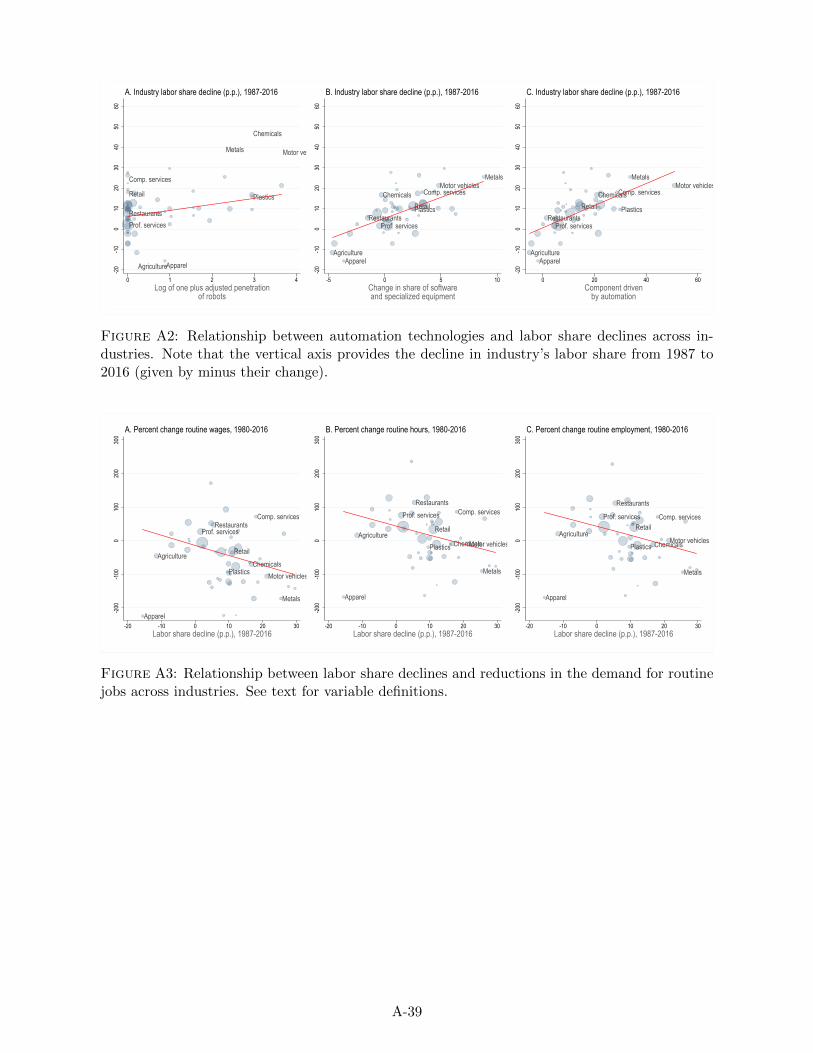
ApparelAgriculture

Prof. servicesRestaurants

PlasticsRetail

Comp. services

Motor vehicles

Chemicals

Metals

-20

-10

010

2030

4050

60

0 1 2 3 4Log of one plus adjusted penetration

of robots

A. Industry labor share decline (p.p.), 1987-2016

ApparelAgriculture

Prof. servicesRestaurants

PlasticsRetail

Comp. servicesMotor vehicles

Chemicals

Metals

-20

-10

010

2030

4050

60

-5 0 5 10Change in share of softwareand specialized equipment

B. Industry labor share decline (p.p.), 1987-2016

ApparelAgriculture

Prof. servicesRestaurants

PlasticsRetail

Comp. servicesMotor vehicles

Chemicals

Metals

-20

-10

010

2030

4050

60

0 20 40 60Component driven

by automation

C. Industry labor share decline (p.p.), 1987-2016

Figure A2: Relationship between automation technologies and labor share declines across in-dustries. Note that the vertical axis provides the decline in industry’s labor share from 1987 to2016 (given by minus their change).

Agriculture

Apparel

Chemicals

Comp. services

Motor vehiclesPlastics

Metals

Prof. servicesRestaurants

Retail

-200

-100

010

020

030

0

-20 -10 0 10 20 30Labor share decline (p.p.), 1987-2016

A. Percent change routine wages, 1980-2016

Agriculture

Apparel

Chemicals

Comp. services

Motor vehiclesPlastics

Metals

Prof. servicesRestaurants

Retail

-200

-100

010

020

030

0

-20 -10 0 10 20 30Labor share decline (p.p.), 1987-2016

B. Percent change routine hours, 1980-2016

Agriculture

Apparel

Chemicals

Comp. services

Motor vehiclesPlastics

Metals

Prof. services

Restaurants

Retail-2

00-1

000

100

200

300

-20 -10 0 10 20 30Labor share decline (p.p.), 1987-2016

C. Percent change routine employment, 1980-2016

Figure A3: Relationship between labor share declines and reductions in the demand for routinejobs across industries. See text for variable definitions.

A-39

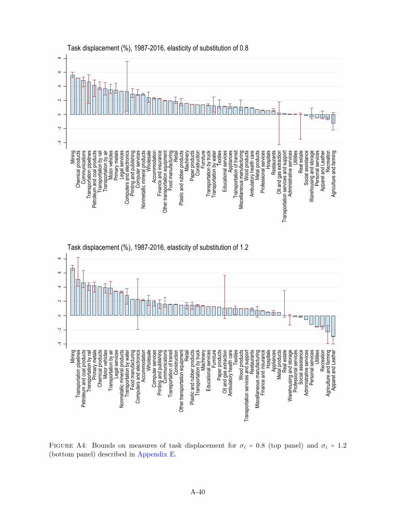
-.4-.2

0.2

.4.6

.8

Minin

gCh

emica

l pro

ducts

Comm

unica

tions

Tran

spor

tation

pipe

lines

Petro

leum

and c

oal p

rodu

ctsTr

ansp

ortat

ion by

rail

Tran

spor

tation

by ai

rMo

tor ve

hicles

Prim

ary m

etals

Lega

l ser

vices

Comp

uters

and e

lectro

nics

Print

ing an

d pub

lishin

gCo

mpute

r ser

vices

Nonm

etallic

mine

ral p

rodu

ctsW

holes

aleAc

comm

odati

onFin

ance

and i

nsur

ance

Othe

r tra

nspo

rtatio

n equ

ipmen

tFo

od m

anufa

cturin

gRe

tail

Plas

tic an

d rub

ber p

rodu

ctsMa

chine

ryPa

per p

rodu

ctsCo

nstru

ction

Furn

iture

Tran

spor

tation

by tr

uck

Tran

spor

tation

by w

ater

Texti

lesEd

ucati

onal

servi

ces

Appli

ance

sTr

ansp

ortat

ion of

tran

sitMi

scell

aneo

us m

anufa

cturin

gW

ood p

rodu

ctsAm

bulat

ory h

ealth

care

Metal

prod

ucts

Profe

ssion

al se

rvice

sHo

spita

lsRe

staur

ants

Oil a

nd ga

s extr

actio

nTr

ansp

ortat

ion se

rvice

s and

supp

ort

Admi

nistra

tive s

ervic

esUt

ilities

Real

estat

eSo

cial a

ssist

ance

War

ehou

sing a

nd st

orag

ePe

rsona

l ser

vices

Appa

rel a

nd Le

ather

Recre

ation

Agric

ultur

e and

farm

ing

Task displacement (%), 1987-2016, elasticity of substitution of 0.8-.4

-.20

.2.4

.6.8

Minin

gTr

ansp

ortat

ion pi

pelin

esPe

troleu

m an

d coa

l pro

ducts

Tran

spor

tation

by ra

ilPr

imar

y meta

lsCh

emica

l pro

ducts

Motor

vehic

lesTr

ansp

ortat

ion by

air

Lega

l ser

vices

Nonm

etallic

mine

ral p

rodu

ctsTr

ansp

ortat

ion by

wate

rFo

od m

anufa

cturin

gCo

mpute

rs an

d elec

tronic

sAc

comm

odati

onW

holes

aleCo

mpute

r ser

vices

Print

ing an

d pub

lishin

gCo

mmun

icatio

nsTr

ansp

ortat

ion of

tran

sitCo

nstru

ction

Othe

r tra

nspo

rtatio

n equ

ipmen

tRe

tail

Plas

tic an

d rub

ber p

rodu

ctsTr

ansp

ortat

ion by

truc

kMa

chine

ryEd

ucati

onal

servi

ces

Furn

iture

Pape

r pro

ducts

Oil a

nd ga

s extr

actio

nAm

bulat

ory h

ealth

care

Texti

lesW

ood p

rodu

ctsTr

ansp

ortat

ion se

rvice

s and

supp

ort

Resta

uran

tsMi

scell

aneo

us m

anufa

cturin

gFin

ance

and i

nsur

ance

Hosp

itals

Appli

ance

sMe

tal pr

oduc

tsRe

al es

tate

War

ehou

sing a

nd st

orag

ePr

ofess

ional

servi

ces

Socia

l ass

istan

ceAd

minis

trativ

e ser

vices

Perso

nal s

ervic

esUt

ilities

Recre

ation

Agric

ultur

e and

farm

ingAp

pare

l and

Leath

er

Task displacement (%), 1987-2016, elasticity of substitution of 1.2

Figure A4: Bounds on measures of task displacement for σi = 0.8 (top panel) and σi = 1.2(bottom panel) described in Appendix E.

A-40

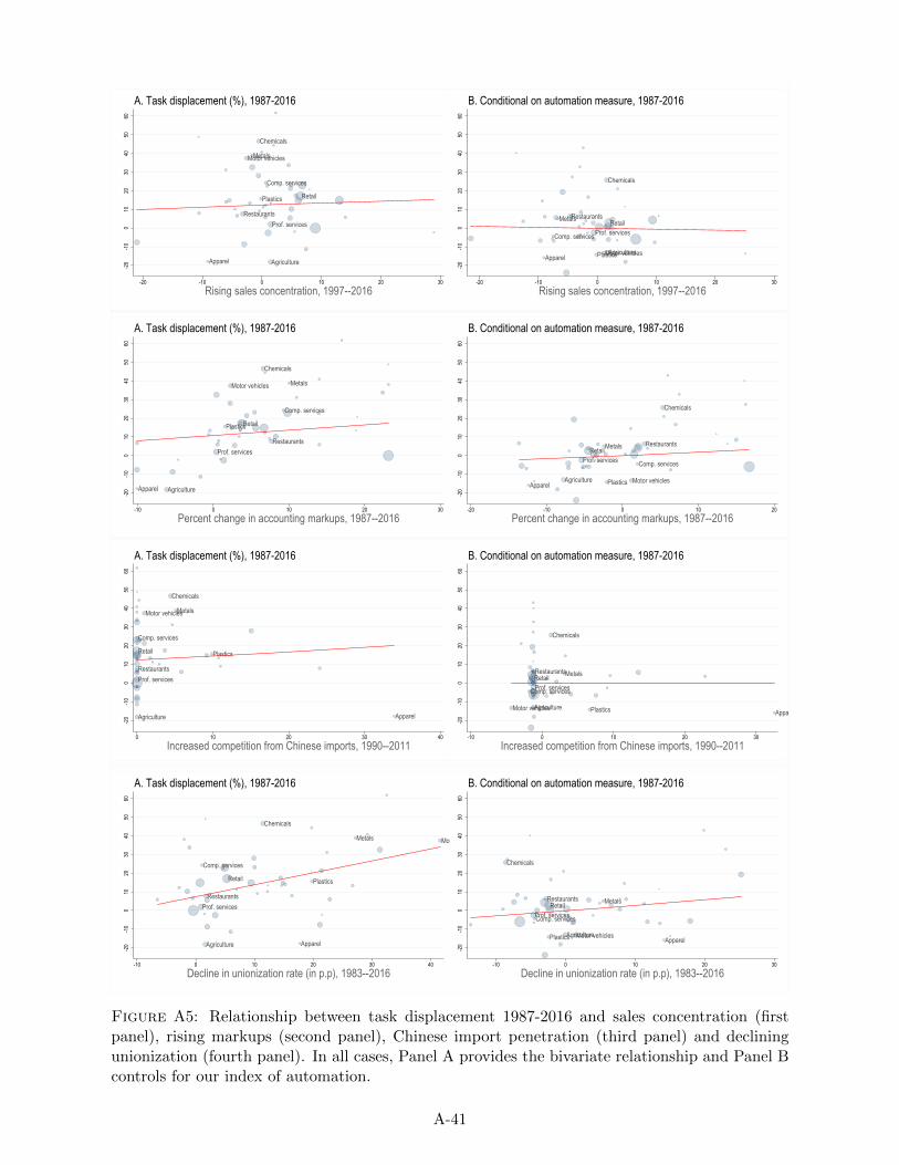
Apparel Agriculture

Prof. servicesRestaurants

Plastics Retail

Comp. services

Motor vehicles

Chemicals

Metals

-20

-10

010

2030

4050

60

-20 -10 0 10 20 30

Rising sales concentration, 1997--2016

A. Task displacement (%), 1987-2016

ApparelAgriculture

Prof. services

Restaurants

Plastics

Retail

Comp. services

Motor vehicles

Chemicals

Metals

-20

-10

010

2030

4050

60

-20 -10 0 10 20 30

Rising sales concentration, 1997--2016

B. Conditional on automation measure, 1987-2016

Apparel Agriculture

Prof. servicesRestaurants

PlasticsRetail

Comp. services

Motor vehicles

Chemicals

Metals

-20

-10

010

2030

4050

60

-10 0 10 20 30

Percent change in accounting markups, 1987--2016

A. Task displacement (%), 1987-2016

ApparelAgriculture

Prof. services

Restaurants

Plastics

Retail

Comp. services

Motor vehicles

Chemicals

Metals

-20

-10

010

2030

4050

60

-20 -10 0 10 20

Percent change in accounting markups, 1987--2016

B. Conditional on automation measure, 1987-2016

ApparelAgriculture

Prof. servicesRestaurants

PlasticsRetail

Comp. services

Motor vehicles

Chemicals

Metals

-20

-10

010

2030

4050

60

0 10 20 30 40

Increased competition from Chinese imports, 1990--2011

A. Task displacement (%), 1987-2016

ApparelAgriculture

Prof. services

Restaurants

Plastics

Retail

Comp. services

Motor vehicles

Chemicals

Metals

-20

-10

010

2030

4050

60

-10 0 10 20 30

Increased competition from Chinese imports, 1990--2011

B. Conditional on automation measure, 1987-2016

ApparelAgriculture

Prof. servicesRestaurants

PlasticsRetail

Comp. services

Motor vehicles

Chemicals

Metals

-20

-10

010

2030

4050

60

-10 0 10 20 30 40

Decline in unionization rate (in p.p), 1983--2016

A. Task displacement (%), 1987-2016

ApparelAgriculture

Prof. services

Restaurants

Plastics

Retail

Comp. services

Motor vehicles

Chemicals

Metals

-20

-10

010

2030

4050

60

-10 0 10 20 30

Decline in unionization rate (in p.p), 1983--2016

B. Conditional on automation measure, 1987-2016

Figure A5: Relationship between task displacement 1987-2016 and sales concentration (firstpanel), rising markups (second panel), Chinese import penetration (third panel) and decliningunionization (fourth panel). In all cases, Panel A provides the bivariate relationship and Panel Bcontrols for our index of automation.

A-41

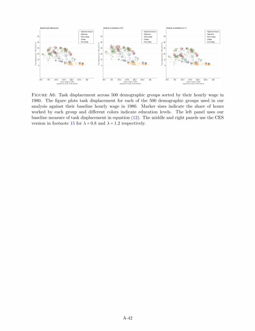
0

10

20

30

40

50Ta

sk di

splac

emen

t, 198

0-20

16 (%

)

$7.5 $10 $13.3 $17.8 $23.7 $31.6 $42Hourly wage in 1980

(logarithmic scale, 2008 dollars)

Highschool dropoutHighschoolSome collegeCollegePost college

Baseline task displacement

0

10

20

30

40

50

Task

disp

lacem

ent, 1

980-

2016

(%)

$7.5 $10 $13.3 $17.8 $23.7 $31.6 $42Hourly wage in 1980

(logarithmic scale, 2008 dollars)

Highschool dropoutHighschoolSome collegeCollegePost college

Elasticity of substitution of 0.8

0

10

20

30

40

50

Task

disp

lacem

ent, 1

980-

2016

(%)

$7.5 $10 $13.3 $17.8 $23.7 $31.6 $42Hourly wage in 1980

(logarithmic scale, 2008 dollars)

Highschool dropoutHighschoolSome collegeCollegePost college

Elasticity of substitution of 1.2

Figure A6: Task displacement across 500 demographic groups sorted by their hourly wage in1980. The figure plots task displacement for each of the 500 demographic groups used in ouranalysis against their baseline hourly wage in 1980. Marker sizes indicate the share of hoursworked by each group and different colors indicate education levels. The left panel uses ourbaseline measure of task displacement in equation (12). The middle and right panels use the CESversion in footnote 15 for λ = 0.8 and λ = 1.2 respectively.

A-42

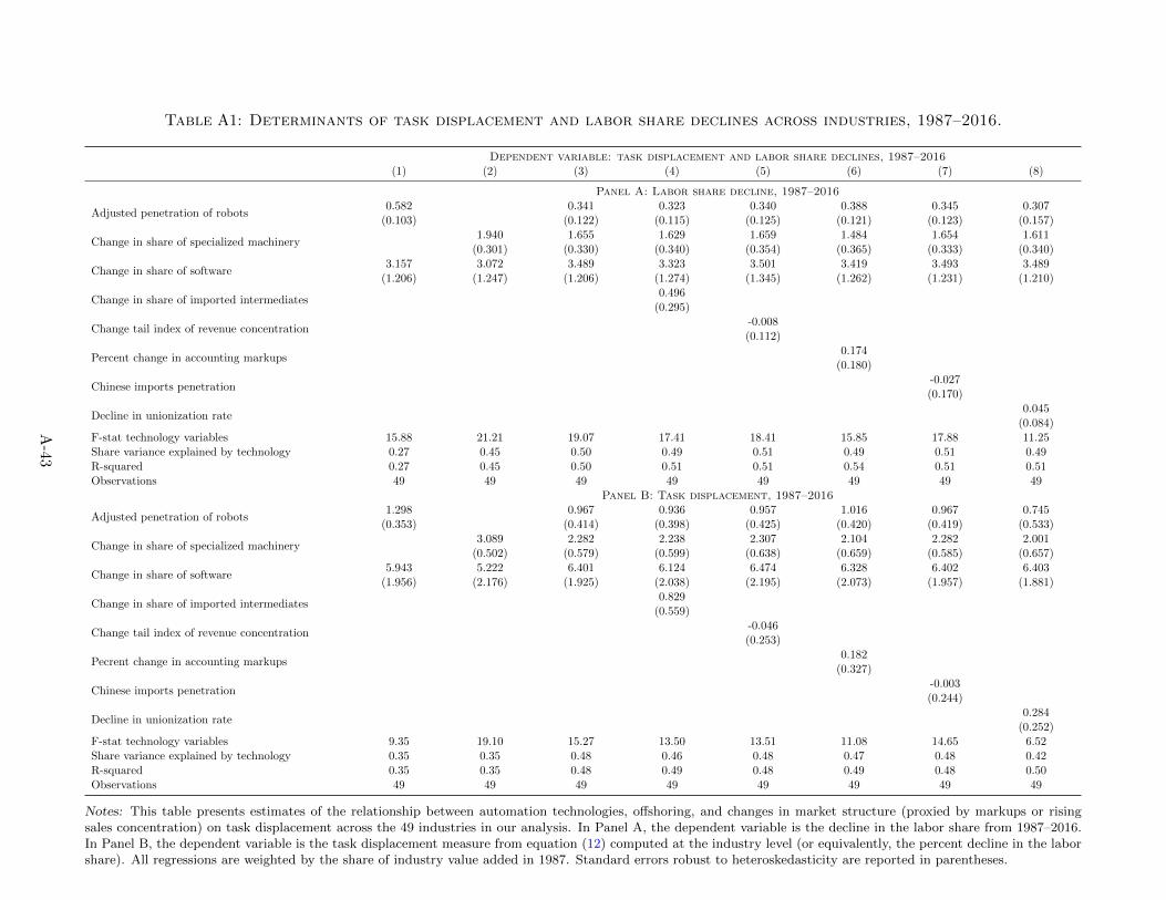
Table A1: Determinants of task displacement and labor share declines across industries, 1987–2016.

Dependent variable: task displacement and labor share declines, 1987–2016(1) (2) (3) (4) (5) (6) (7) (8)

Panel A: Labor share decline, 1987–2016

Adjusted penetration of robots0.582 0.341 0.323 0.340 0.388 0.345 0.307

(0.103) (0.122) (0.115) (0.125) (0.121) (0.123) (0.157)

Change in share of specialized machinery1.940 1.655 1.629 1.659 1.484 1.654 1.611

(0.301) (0.330) (0.340) (0.354) (0.365) (0.333) (0.340)

Change in share of software3.157 3.072 3.489 3.323 3.501 3.419 3.493 3.489

(1.206) (1.247) (1.206) (1.274) (1.345) (1.262) (1.231) (1.210)

Change in share of imported intermediates0.496

(0.295)

Change tail index of revenue concentration-0.008(0.112)

Percent change in accounting markups0.174

(0.180)

Chinese imports penetration-0.027(0.170)

Decline in unionization rate0.045

(0.084)F-stat technology variables 15.88 21.21 19.07 17.41 18.41 15.85 17.88 11.25Share variance explained by technology 0.27 0.45 0.50 0.49 0.51 0.49 0.51 0.49R-squared 0.27 0.45 0.50 0.51 0.51 0.54 0.51 0.51Observations 49 49 49 49 49 49 49 49

Panel B: Task displacement, 1987–2016

Adjusted penetration of robots1.298 0.967 0.936 0.957 1.016 0.967 0.745

(0.353) (0.414) (0.398) (0.425) (0.420) (0.419) (0.533)

Change in share of specialized machinery3.089 2.282 2.238 2.307 2.104 2.282 2.001

(0.502) (0.579) (0.599) (0.638) (0.659) (0.585) (0.657)

Change in share of software5.943 5.222 6.401 6.124 6.474 6.328 6.402 6.403

(1.956) (2.176) (1.925) (2.038) (2.195) (2.073) (1.957) (1.881)

Change in share of imported intermediates0.829

(0.559)

Change tail index of revenue concentration-0.046(0.253)

Pecrent change in accounting markups0.182

(0.327)

Chinese imports penetration-0.003(0.244)

Decline in unionization rate0.284

(0.252)F-stat technology variables 9.35 19.10 15.27 13.50 13.51 11.08 14.65 6.52Share variance explained by technology 0.35 0.35 0.48 0.46 0.48 0.47 0.48 0.42R-squared 0.35 0.35 0.48 0.49 0.48 0.49 0.48 0.50Observations 49 49 49 49 49 49 49 49

Notes: This table presents estimates of the relationship between automation technologies, offshoring, and changes in market structure (proxied by markups or risingsales concentration) on task displacement across the 49 industries in our analysis. In Panel A, the dependent variable is the decline in the labor share from 1987–2016.In Panel B, the dependent variable is the task displacement measure from equation (12) computed at the industry level (or equivalently, the percent decline in the laborshare). All regressions are weighted by the share of industry value added in 1987. Standard errors robust to heteroskedasticity are reported in parentheses.

A-43

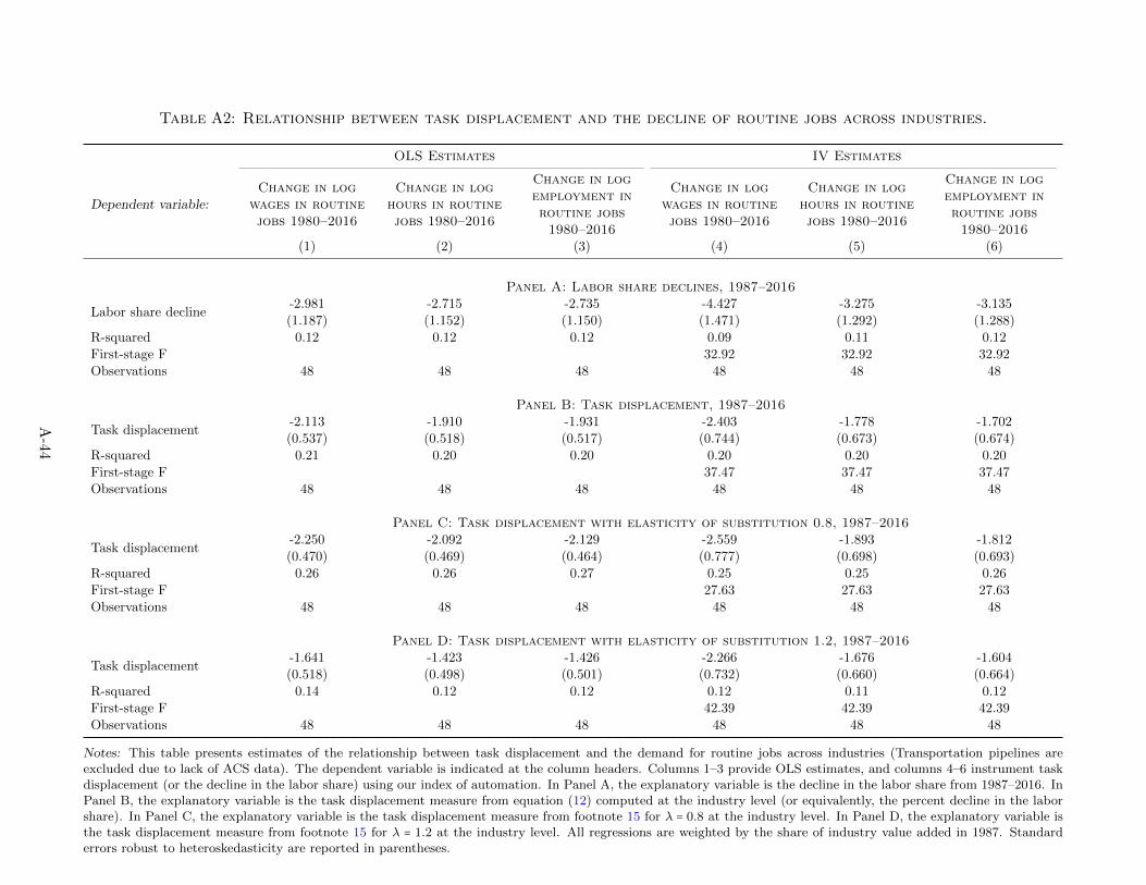
Table A2: Relationship between task displacement and the decline of routine jobs across industries.

OLS Estimates IV Estimates

Dependent variable:Change in log

wages in routinejobs 1980–2016

Change in loghours in routinejobs 1980–2016

Change in logemployment inroutine jobs

1980–2016

Change in logwages in routinejobs 1980–2016

Change in loghours in routinejobs 1980–2016

Change in logemployment inroutine jobs

1980–2016(1) (2) (3) (4) (5) (6)

Panel A: Labor share declines, 1987–2016

Labor share decline-2.981 -2.715 -2.735 -4.427 -3.275 -3.135(1.187) (1.152) (1.150) (1.471) (1.292) (1.288)

R-squared 0.12 0.12 0.12 0.09 0.11 0.12First-stage F 32.92 32.92 32.92Observations 48 48 48 48 48 48

Panel B: Task displacement, 1987–2016

Task displacement-2.113 -1.910 -1.931 -2.403 -1.778 -1.702(0.537) (0.518) (0.517) (0.744) (0.673) (0.674)

R-squared 0.21 0.20 0.20 0.20 0.20 0.20First-stage F 37.47 37.47 37.47Observations 48 48 48 48 48 48

Panel C: Task displacement with elasticity of substitution 0.8, 1987–2016

Task displacement-2.250 -2.092 -2.129 -2.559 -1.893 -1.812(0.470) (0.469) (0.464) (0.777) (0.698) (0.693)

R-squared 0.26 0.26 0.27 0.25 0.25 0.26First-stage F 27.63 27.63 27.63Observations 48 48 48 48 48 48

Panel D: Task displacement with elasticity of substitution 1.2, 1987–2016

Task displacement-1.641 -1.423 -1.426 -2.266 -1.676 -1.604(0.518) (0.498) (0.501) (0.732) (0.660) (0.664)

R-squared 0.14 0.12 0.12 0.12 0.11 0.12First-stage F 42.39 42.39 42.39Observations 48 48 48 48 48 48

Notes: This table presents estimates of the relationship between task displacement and the demand for routine jobs across industries (Transportation pipelines areexcluded due to lack of ACS data). The dependent variable is indicated at the column headers. Columns 1–3 provide OLS estimates, and columns 4–6 instrument taskdisplacement (or the decline in the labor share) using our index of automation. In Panel A, the explanatory variable is the decline in the labor share from 1987–2016. InPanel B, the explanatory variable is the task displacement measure from equation (12) computed at the industry level (or equivalently, the percent decline in the laborshare). In Panel C, the explanatory variable is the task displacement measure from footnote 15 for λ = 0.8 at the industry level. In Panel D, the explanatory variable isthe task displacement measure from footnote 15 for λ = 1.2 at the industry level. All regressions are weighted by the share of industry value added in 1987. Standarderrors robust to heteroskedasticity are reported in parentheses.

A-44

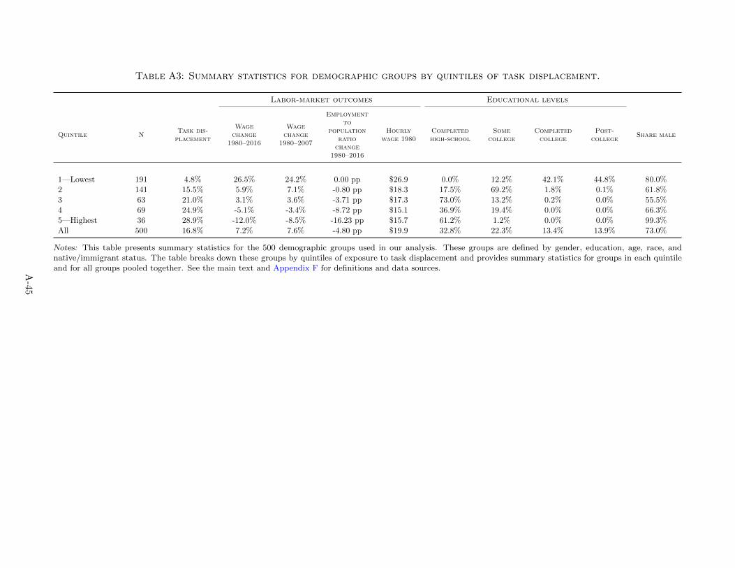
Table A3: Summary statistics for demographic groups by quintiles of task displacement.

Labor-market outcomes Educational levels

Quintile NTask dis-

placement

Wagechange

1980–2016

Wagechange

1980–2007

Employmentto

populationratio

change1980–2016

Hourlywage 1980

Completedhigh-school

Somecollege

Completedcollege

Post-college

Share male

1—Lowest 191 4.8% 26.5% 24.2% 0.00 pp $26.9 0.0% 12.2% 42.1% 44.8% 80.0%2 141 15.5% 5.9% 7.1% -0.80 pp $18.3 17.5% 69.2% 1.8% 0.1% 61.8%3 63 21.0% 3.1% 3.6% -3.71 pp $17.3 73.0% 13.2% 0.2% 0.0% 55.5%4 69 24.9% -5.1% -3.4% -8.72 pp $15.1 36.9% 19.4% 0.0% 0.0% 66.3%5—Highest 36 28.9% -12.0% -8.5% -16.23 pp $15.7 61.2% 1.2% 0.0% 0.0% 99.3%All 500 16.8% 7.2% 7.6% -4.80 pp $19.9 32.8% 22.3% 13.4% 13.9% 73.0%

Notes: This table presents summary statistics for the 500 demographic groups used in our analysis. These groups are defined by gender, education, age, race, andnative/immigrant status. The table breaks down these groups by quintiles of exposure to task displacement and provides summary statistics for groups in each quintileand for all groups pooled together. See the main text and Appendix F for definitions and data sources.A

-45

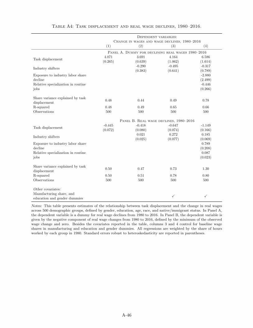
Table A4: Task displacement and real wage declines, 1980–2016.

Dependent variables:Change in wages and wage declines, 1980–2016

(1) (2) (3) (4)

Panel A. Dummy for declining real wages 1980–2016

Task displacement4.071 3.691 4.164 6.586

(0.265) (0.639) (1.062) (1.614)

Industry shifters-0.290 -0.495 -0.317(0.383) (0.641) (0.789)

Exposure to industry labor sharedecline

-2.880(2.499)

Relative specialization in routinejobs

-0.446(0.266)

Share variance explained by taskdisplacement

0.48 0.44 0.49 0.78

R-squared 0.48 0.49 0.65 0.66Observations 500 500 500 500

Panel B. Real wage declines, 1980–2016

Task displacement-0.445 -0.418 -0.647 -1.149(0.072) (0.080) (0.074) (0.166)

Industry shifters0.021 0.272 0.185

(0.025) (0.077) (0.069)Exposure to industry labor sharedecline

0.789(0.208)

Relative specialization in routinejobs

0.087(0.023)

Share variance explained by taskdisplacement

0.50 0.47 0.73 1.30

R-squared 0.50 0.51 0.78 0.80Observations 500 500 500 500

Other covariates:Manufacturing share, andeducation and gender dummies

✓ ✓

Notes: This table presents estimates of the relationship between task displacement and the change in real wagesacross 500 demographic groups, defined by gender, education, age, race, and native/immigrant status. In Panel A,the dependent variable is a dummy for real wage declines from 1980 to 2016. In Panel B, the dependent variable isgiven by the negative component of real wage changes from 1980 to 2016, defined by the minimum of the observedwage change and zero. Besides the covariates reported in the table, columns 3 and 4 control for baseline wageshares in manufacturing and education and gender dummies. All regressions are weighted by the share of hoursworked by each group in 1980. Standard errors robust to heteroskedasticity are reported in parentheses.

A-46

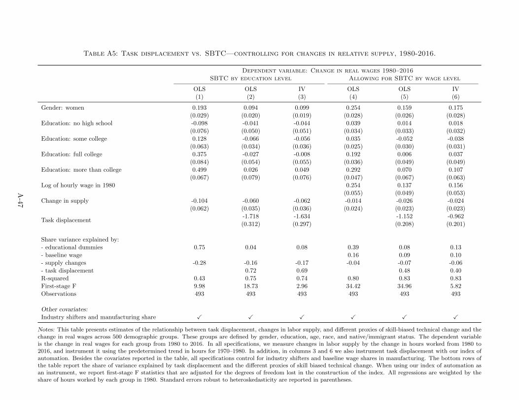
Table A5: Task displacement vs. SBTC—controlling for changes in relative supply, 1980-2016.

Dependent variable: Change in real wages 1980–2016SBTC by education level Allowing for SBTC by wage level

OLS OLS IV OLS OLS IV(1) (2) (3) (4) (5) (6)

Gender: women 0.193 0.094 0.099 0.254 0.159 0.175(0.029) (0.020) (0.019) (0.028) (0.026) (0.028)

Education: no high school -0.098 -0.041 -0.044 0.039 0.014 0.018(0.076) (0.050) (0.051) (0.034) (0.033) (0.032)

Education: some college 0.128 -0.066 -0.056 0.035 -0.052 -0.038(0.063) (0.034) (0.036) (0.025) (0.030) (0.031)

Education: full college 0.375 -0.027 -0.008 0.192 0.006 0.037(0.084) (0.054) (0.055) (0.036) (0.049) (0.049)

Education: more than college 0.499 0.026 0.049 0.292 0.070 0.107(0.067) (0.079) (0.076) (0.047) (0.067) (0.063)

Log of hourly wage in 1980 0.254 0.137 0.156(0.055) (0.049) (0.053)

Change in supply -0.104 -0.060 -0.062 -0.014 -0.026 -0.024(0.062) (0.035) (0.036) (0.024) (0.023) (0.023)

Task displacement-1.718 -1.634 -1.152 -0.962(0.312) (0.297) (0.208) (0.201)

Share variance explained by:- educational dummies 0.75 0.04 0.08 0.39 0.08 0.13- baseline wage 0.16 0.09 0.10- supply changes -0.28 -0.16 -0.17 -0.04 -0.07 -0.06- task displacement 0.72 0.69 0.48 0.40R-squared 0.43 0.75 0.74 0.80 0.83 0.83First-stage F 9.98 18.73 2.96 34.42 34.96 5.82Observations 493 493 493 493 493 493

Other covariates:Industry shifters and manufacturing share ✓ ✓ ✓ ✓ ✓ ✓

Notes: This table presents estimates of the relationship between task displacement, changes in labor supply, and different proxies of skill-biased technical change and thechange in real wages across 500 demographic groups. These groups are defined by gender, education, age, race, and native/immigrant status. The dependent variableis the change in real wages for each group from 1980 to 2016. In all specifications, we measure changes in labor supply by the change in hours worked from 1980 to2016, and instrument it using the predetermined trend in hours for 1970–1980. In addition, in columns 3 and 6 we also instrument task displacement with our index ofautomation. Besides the covariates reported in the table, all specifications control for industry shifters and baseline wage shares in manufacturing. The bottom rows ofthe table report the share of variance explained by task displacement and the different proxies of skill biased technical change. When using our index of automation asan instrument, we report first-stage F statistics that are adjusted for the degrees of freedom lost in the construction of the index. All regressions are weighted by theshare of hours worked by each group in 1980. Standard errors robust to heteroskedasticity are reported in parentheses.

A-47

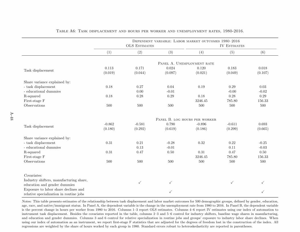
Table A6: Task displacement and hours per worker and unemployment rates, 1980-2016.

Dependent variable: Labor market outcomes 1980–2016OLS Estimates IV Estimates

(1) (2) (3) (4) (5) (6)

Panel A. Unemployment rate

Task displacement0.113 0.171 0.024 0.120 0.183 0.018

(0.019) (0.044) (0.097) (0.021) (0.049) (0.107)

Share variance explained by:- task displacement 0.18 0.27 0.04 0.19 0.29 0.03- educational dummies 0.00 -0.01 -0.00 -0.02R-squared 0.18 0.28 0.29 0.18 0.28 0.29First-stage F 3246.45 785.80 156.33Observations 500 500 500 500 500 500

Panel B. log hours per worker

Task displacement-0.862 -0.581 0.790 -0.896 -0.611 0.693(0.180) (0.292) (0.619) (0.186) (0.299) (0.665)

Share variance explained by:- task displacement 0.31 0.21 -0.28 0.32 0.22 -0.25- educational dummies 0.13 -0.01 0.11 -0.03R-squared 0.31 0.47 0.50 0.31 0.47 0.50First-stage F 3246.45 785.80 156.33Observations 500 500 500 500 500 500

Covariates:Industry shifters, manufacturing share,education and gender dummies

✓ ✓ ✓ ✓

Exposure to labor share declines andrelative specialization in routine jobs

✓ ✓

Notes: This table presents estimates of the relationship between task displacement and labor market outcomes for 500 demographic groups, defined by gender, education,age, race, and native/immigrant status. In Panel A, the dependent variable is the change in the unemployment rate from 1980 to 2016. In Panel B, the dependent variableis the percent change in hours per worker from 1980 to 2016. Columns 1–3 report OLS estimates. Columns 4–6 report IV estimates using our index of automation toinstrument task displacement. Besides the covariates reported in the table, columns 2–3 and 5–6 control for industry shifters, baseline wage shares in manufacturing,and education and gender dummies. Columns 3 and 6 control for relative specialization in routine jobs and groups’ exposure to industry labor share declines. Whenusing our index of automation as an instrument, we report first-stage F statistics that are adjusted for the degrees of freedom lost in the construction of the index. Allregressions are weighted by the share of hours worked by each group in 1980. Standard errors robust to heteroskedasticity are reported in parentheses.

A-48

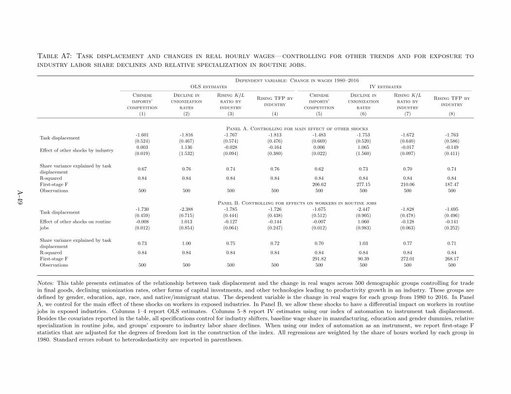
Table A7: Task displacement and changes in real hourly wages—controlling for other trends and for exposure toindustry labor share declines and relative specialization in routine jobs.

Dependent variable: Change in wages 1980–2016OLS estimates IV estimates

Chineseimports’

competition

Decline inunionization

rates

Rising K/Lratio byindustry

Rising TFP byindustry

Chineseimports’

competition

Decline inunionization

rates

Rising K/Lratio byindustry

Rising TFP byindustry

(1) (2) (3) (4) (5) (6) (7) (8)

Panel A. Controlling for main effect of other shocks

Task displacement-1.601 -1.816 -1.767 -1.813 -1.483 -1.753 -1.672 -1.763(0.524) (0.467) (0.574) (0.476) (0.669) (0.520) (0.640) (0.586)

Effect of other shocks by industry0.003 1.136 -0.028 -0.164 0.006 1.065 -0.017 -0.149

(0.019) (1.532) (0.094) (0.380) (0.022) (1.560) (0.097) (0.411)

Share variance explained by taskdisplacement

0.67 0.76 0.74 0.76 0.62 0.73 0.70 0.74

R-squared 0.84 0.84 0.84 0.84 0.84 0.84 0.84 0.84First-stage F 206.62 277.15 210.06 187.47Observations 500 500 500 500 500 500 500 500

Panel B. Controlling for effects on workers in routine jobs

Task displacement-1.730 -2.388 -1.785 -1.726 -1.675 -2.447 -1.828 -1.695(0.459) (0.715) (0.444) (0.438) (0.512) (0.905) (0.478) (0.496)

Effect of other shocks on routinejobs

-0.008 1.013 -0.127 -0.144 -0.007 1.060 -0.128 -0.141(0.012) (0.854) (0.064) (0.247) (0.012) (0.983) (0.063) (0.252)

Share variance explained by taskdisplacement

0.73 1.00 0.75 0.72 0.70 1.03 0.77 0.71

R-squared 0.84 0.84 0.84 0.84 0.84 0.84 0.84 0.84First-stage F 291.82 90.39 272.01 268.17Observations 500 500 500 500 500 500 500 500

Notes: This table presents estimates of the relationship between task displacement and the change in real wages across 500 demographic groups controlling for tradein final goods, declining unionization rates, other forms of capital investments, and other technologies leading to productivity growth in an industry. These groups aredefined by gender, education, age, race, and native/immigrant status. The dependent variable is the change in real wages for each group from 1980 to 2016. In PanelA, we control for the main effect of these shocks on workers in exposed industries. In Panel B, we allow these shocks to have a differential impact on workers in routinejobs in exposed industries. Columns 1–4 report OLS estimates. Columns 5–8 report IV estimates using our index of automation to instrument task displacement.Besides the covariates reported in the table, all specifications control for industry shifters, baseline wage share in manufacturing, education and gender dummies, relativespecialization in routine jobs, and groups’ exposure to industry labor share declines. When using our index of automation as an instrument, we report first-stage Fstatistics that are adjusted for the degrees of freedom lost in the construction of the index. All regressions are weighted by the share of hours worked by each group in1980. Standard errors robust to heteroskedasticity are reported in parentheses.

A-49

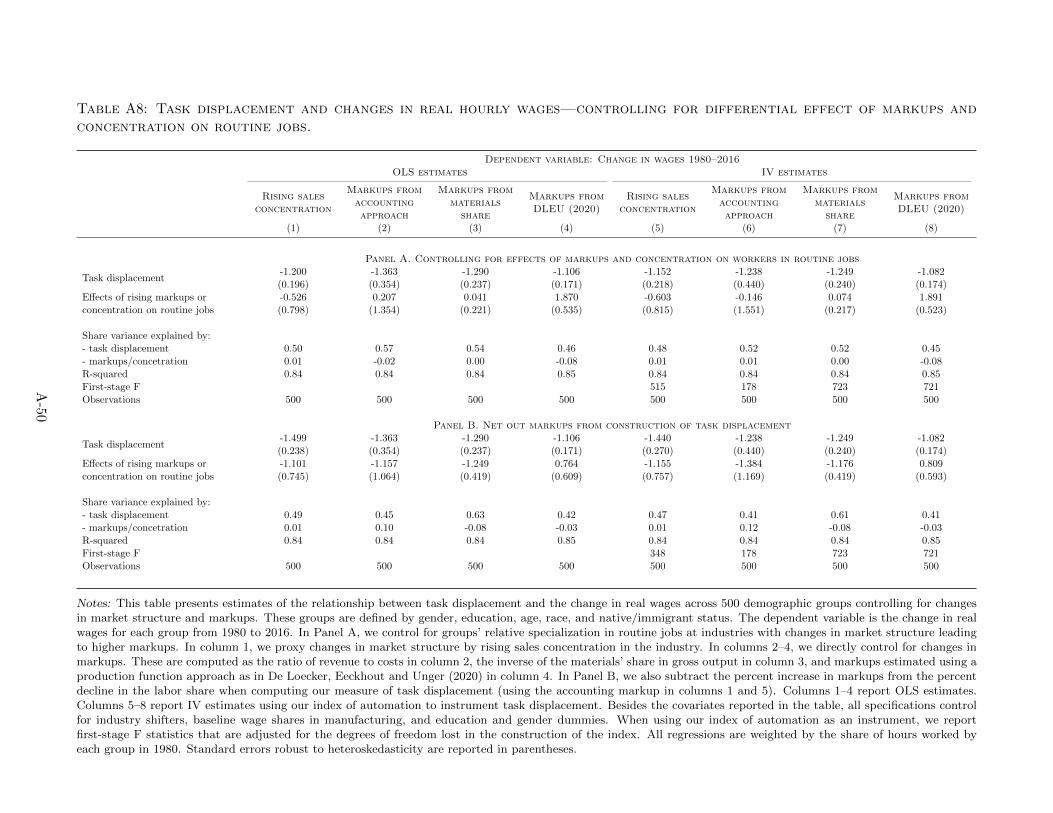
Table A8: Task displacement and changes in real hourly wages—controlling for differential effect of markups andconcentration on routine jobs.

Dependent variable: Change in wages 1980–2016OLS estimates IV estimates

Rising salesconcentration

Markups fromaccountingapproach

Markups frommaterials

share

Markups fromDLEU (2020)

Rising salesconcentration

Markups fromaccountingapproach

Markups frommaterials

share

Markups fromDLEU (2020)

(1) (2) (3) (4) (5) (6) (7) (8)

Panel A. Controlling for effects of markups and concentration on workers in routine jobs

Task displacement-1.200 -1.363 -1.290 -1.106 -1.152 -1.238 -1.249 -1.082(0.196) (0.354) (0.237) (0.171) (0.218) (0.440) (0.240) (0.174)

Effects of rising markups orconcentration on routine jobs

-0.526 0.207 0.041 1.870 -0.603 -0.146 0.074 1.891(0.798) (1.354) (0.221) (0.535) (0.815) (1.551) (0.217) (0.523)

Share variance explained by:- task displacement 0.50 0.57 0.54 0.46 0.48 0.52 0.52 0.45- markups/concetration 0.01 -0.02 0.00 -0.08 0.01 0.01 0.00 -0.08R-squared 0.84 0.84 0.84 0.85 0.84 0.84 0.84 0.85First-stage F 515 178 723 721Observations 500 500 500 500 500 500 500 500

Panel B. Net out markups from construction of task displacement

Task displacement-1.499 -1.363 -1.290 -1.106 -1.440 -1.238 -1.249 -1.082(0.238) (0.354) (0.237) (0.171) (0.270) (0.440) (0.240) (0.174)

Effects of rising markups orconcentration on routine jobs

-1.101 -1.157 -1.249 0.764 -1.155 -1.384 -1.176 0.809(0.745) (1.064) (0.419) (0.609) (0.757) (1.169) (0.419) (0.593)

Share variance explained by:- task displacement 0.49 0.45 0.63 0.42 0.47 0.41 0.61 0.41- markups/concetration 0.01 0.10 -0.08 -0.03 0.01 0.12 -0.08 -0.03R-squared 0.84 0.84 0.84 0.85 0.84 0.84 0.84 0.85First-stage F 348 178 723 721Observations 500 500 500 500 500 500 500 500

Notes: This table presents estimates of the relationship between task displacement and the change in real wages across 500 demographic groups controlling for changesin market structure and markups. These groups are defined by gender, education, age, race, and native/immigrant status. The dependent variable is the change in realwages for each group from 1980 to 2016. In Panel A, we control for groups’ relative specialization in routine jobs at industries with changes in market structure leadingto higher markups. In column 1, we proxy changes in market structure by rising sales concentration in the industry. In columns 2–4, we directly control for changes inmarkups. These are computed as the ratio of revenue to costs in column 2, the inverse of the materials’ share in gross output in column 3, and markups estimated using aproduction function approach as in De Loecker, Eeckhout and Unger (2020) in column 4. In Panel B, we also subtract the percent increase in markups from the percentdecline in the labor share when computing our measure of task displacement (using the accounting markup in columns 1 and 5). Columns 1–4 report OLS estimates.Columns 5–8 report IV estimates using our index of automation to instrument task displacement. Besides the covariates reported in the table, all specifications controlfor industry shifters, baseline wage shares in manufacturing, and education and gender dummies. When using our index of automation as an instrument, we reportfirst-stage F statistics that are adjusted for the degrees of freedom lost in the construction of the index. All regressions are weighted by the share of hours worked byeach group in 1980. Standard errors robust to heteroskedasticity are reported in parentheses.

A-50

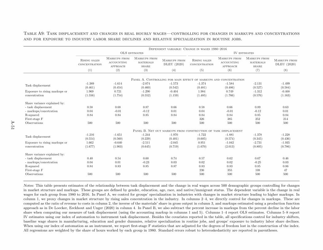
Table A9: Task displacement and changes in real hourly wages—controlling for changes in markups and concentrationsand for exposure to industry labor share declines and relative specialization in routine jobs.

Dependent variable: Change in wages 1980–2016OLS estimates IV estimates

Rising salesconcentration

Markups fromaccountingapproach

Markups frommaterials

share

Markups fromDLEU (2020)

Rising salesconcentration

Markups fromaccountingapproach

Markups frommaterials

share

Markups fromDLEU (2020)

(1) (2) (3) (4) (5) (6) (7) (8)

Panel A. Controlling for main effect of markups and concentration

Task displacement-1.389 -1.614 -2.074 -1.573 -1.374 -1.584 -2.131 -1.499(0.461) (0.454) (0.460) (0.542) (0.481) (0.486) (0.527) (0.584)

Exposure to rising markups orconcentration

1.969 0.721 -1.290 -0.404 1.984 0.749 -1.312 -0.468(1.556) (1.754) (0.552) (1.159) (1.485) (1.766) (0.576) (1.163)

Share variance explained by:- task displacement 0.58 0.68 0.87 0.66 0.58 0.66 0.89 0.63- markups/concetration 0.04 -0.01 -0.12 0.01 0.04 -0.01 -0.12 0.01R-squared 0.84 0.84 0.85 0.84 0.84 0.84 0.85 0.84First-stage F 326 385 252 214Observations 500 500 500 500 500 500 500 500

Panel B. Net out markups from construction of task displacement

Task displacement-1.216 -1.651 -1.244 -1.970 -1.722 -1.881 -1.378 -1.228(0.554) (0.560) (0.229) (0.401) (0.605) (0.574) (0.345) (0.436)

Exposure to rising markups orconcentration

1.662 -0.640 -2.511 -2.045 0.951 -1.042 -2.731 -1.935(1.677) (1.903) (0.645) (0.719) (1.670) (2.013) (0.805) (0.786)

Share variance explained by:- task displacement 0.40 0.54 0.60 0.74 0.57 0.62 0.67 0.46- markups/concetration 0.04 0.01 -0.23 0.03 0.02 0.02 -0.25 0.03R-squared 0.84 0.83 0.85 0.87 0.83 0.83 0.85 0.86First-stage F 236 355 108 47Observations 500 500 500 500 500 500 500 500

Notes: This table presents estimates of the relationship between task displacement and the change in real wages across 500 demographic groups controlling for changesin market structure and markups. These groups are defined by gender, education, age, race, and native/immigrant status. The dependent variable is the change in realwages for each group from 1980 to 2016. In Panel A, we control for groups’ specialization in industries with changes in market structure leading to higher markups. Incolumn 1, we proxy changes in market structure by rising sales concentration in the industry. In columns 2–4, we directly control for changes in markups. These arecomputed as the ratio of revenue to costs in column 2, the inverse of the materials’ share in gross output in column 3, and markups estimated using a production functionapproach as in De Loecker, Eeckhout and Unger (2020) in column 4. In Panel B, we also subtract the percent increase in markups from the percent decline in the laborshare when computing our measure of task displacement (using the accounting markup in columns 1 and 5). Columns 1–4 report OLS estimates. Columns 5–8 reportIV estimates using our index of automation to instrument task displacement. Besides the covariates reported in the table, all specifications control for industry shifters,baseline wage shares in manufacturing, education and gender dummies, relative specialization in routine jobs, and groups’ exposure to industry labor share declines.When using our index of automation as an instrument, we report first-stage F statistics that are adjusted for the degrees of freedom lost in the construction of the index.All regressions are weighted by the share of hours worked by each group in 1980. Standard errors robust to heteroskedasticity are reported in parentheses.

A-51

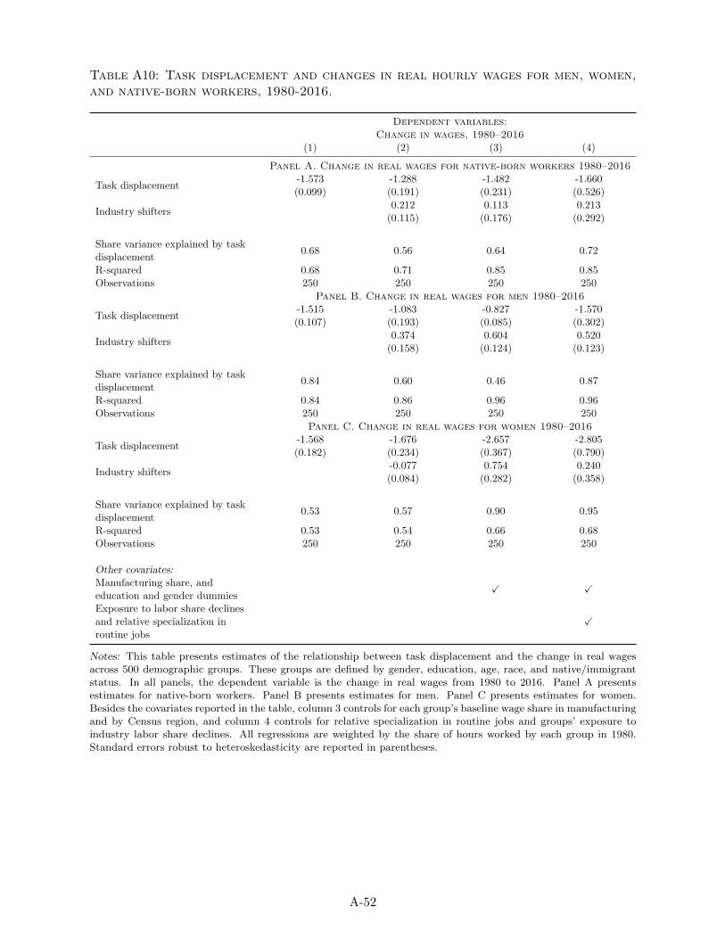
Table A10: Task displacement and changes in real hourly wages for men, women,and native-born workers, 1980-2016.

Dependent variables:Change in wages, 1980–2016

(1) (2) (3) (4)

Panel A. Change in real wages for native-born workers 1980–2016

Task displacement-1.573 -1.288 -1.482 -1.660(0.099) (0.191) (0.231) (0.526)

Industry shifters0.212 0.113 0.213

(0.115) (0.176) (0.292)

Share variance explained by taskdisplacement

0.68 0.56 0.64 0.72

R-squared 0.68 0.71 0.85 0.85Observations 250 250 250 250

Panel B. Change in real wages for men 1980–2016

Task displacement-1.515 -1.083 -0.827 -1.570(0.107) (0.193) (0.085) (0.302)

Industry shifters0.374 0.604 0.520

(0.158) (0.124) (0.123)

Share variance explained by taskdisplacement

0.84 0.60 0.46 0.87

R-squared 0.84 0.86 0.96 0.96Observations 250 250 250 250

Panel C. Change in real wages for women 1980–2016

Task displacement-1.568 -1.676 -2.657 -2.805(0.182) (0.234) (0.367) (0.790)

Industry shifters-0.077 0.754 0.240(0.084) (0.282) (0.358)

Share variance explained by taskdisplacement

0.53 0.57 0.90 0.95

R-squared 0.53 0.54 0.66 0.68Observations 250 250 250 250

Other covariates:Manufacturing share, andeducation and gender dummies

✓ ✓

Exposure to labor share declinesand relative specialization inroutine jobs

✓

Notes: This table presents estimates of the relationship between task displacement and the change in real wagesacross 500 demographic groups. These groups are defined by gender, education, age, race, and native/immigrantstatus. In all panels, the dependent variable is the change in real wages from 1980 to 2016. Panel A presentsestimates for native-born workers. Panel B presents estimates for men. Panel C presents estimates for women.Besides the covariates reported in the table, column 3 controls for each group’s baseline wage share in manufacturingand by Census region, and column 4 controls for relative specialization in routine jobs and groups’ exposure toindustry labor share declines. All regressions are weighted by the share of hours worked by each group in 1980.Standard errors robust to heteroskedasticity are reported in parentheses.

A-52

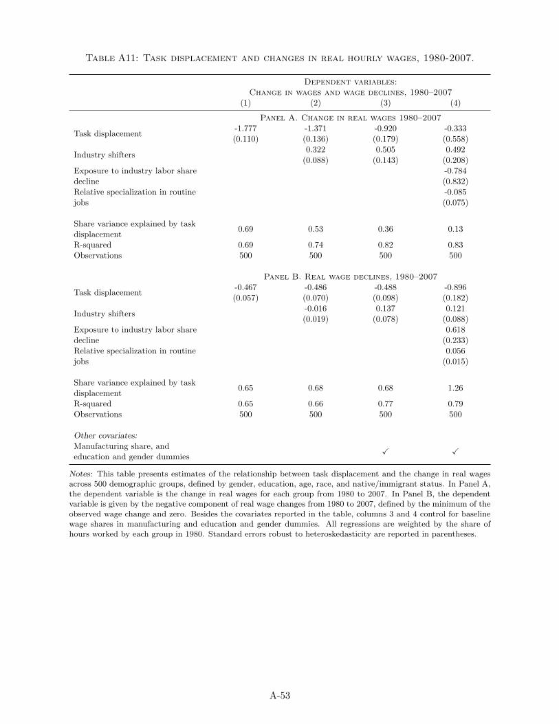
Table A11: Task displacement and changes in real hourly wages, 1980-2007.

Dependent variables:Change in wages and wage declines, 1980–2007

(1) (2) (3) (4)

Panel A. Change in real wages 1980–2007

Task displacement-1.777 -1.371 -0.920 -0.333(0.110) (0.136) (0.179) (0.558)

Industry shifters0.322 0.505 0.492

(0.088) (0.143) (0.208)Exposure to industry labor sharedecline

-0.784(0.832)

Relative specialization in routinejobs

-0.085(0.075)

Share variance explained by taskdisplacement

0.69 0.53 0.36 0.13

R-squared 0.69 0.74 0.82 0.83Observations 500 500 500 500

Panel B. Real wage declines, 1980–2007

Task displacement-0.467 -0.486 -0.488 -0.896(0.057) (0.070) (0.098) (0.182)

Industry shifters-0.016 0.137 0.121(0.019) (0.078) (0.088)

Exposure to industry labor sharedecline

0.618(0.233)

Relative specialization in routinejobs

0.056(0.015)

Share variance explained by taskdisplacement

0.65 0.68 0.68 1.26

R-squared 0.65 0.66 0.77 0.79Observations 500 500 500 500

Other covariates:Manufacturing share, andeducation and gender dummies

✓ ✓

Notes: This table presents estimates of the relationship between task displacement and the change in real wagesacross 500 demographic groups, defined by gender, education, age, race, and native/immigrant status. In Panel A,the dependent variable is the change in real wages for each group from 1980 to 2007. In Panel B, the dependentvariable is given by the negative component of real wage changes from 1980 to 2007, defined by the minimum of theobserved wage change and zero. Besides the covariates reported in the table, columns 3 and 4 control for baselinewage shares in manufacturing and education and gender dummies. All regressions are weighted by the share ofhours worked by each group in 1980. Standard errors robust to heteroskedasticity are reported in parentheses.

A-53

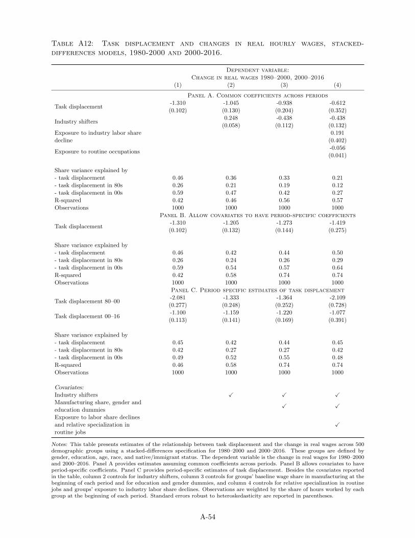
Table A12: Task displacement and changes in real hourly wages, stacked-differences models, 1980-2000 and 2000-2016.

Dependent variable:Change in real wages 1980–2000, 2000–2016

(1) (2) (3) (4)

Panel A. Common coefficients across periods

Task displacement-1.310 -1.045 -0.938 -0.612(0.102) (0.130) (0.204) (0.352)

Industry shifters0.248 -0.438 -0.438

(0.058) (0.112) (0.132)Exposure to industry labor sharedecline

0.191(0.402)

Exposure to routine occupations-0.056(0.041)

Share variance explained by- task displacement 0.46 0.36 0.33 0.21- task displacement in 80s 0.26 0.21 0.19 0.12- task displacement in 00s 0.59 0.47 0.42 0.27R-squared 0.42 0.46 0.56 0.57Observations 1000 1000 1000 1000

Panel B. Allow covariates to have period-specific coefficients

Task displacement-1.310 -1.205 -1.273 -1.419(0.102) (0.132) (0.144) (0.275)

Share variance explained by- task displacement 0.46 0.42 0.44 0.50- task displacement in 80s 0.26 0.24 0.26 0.29- task displacement in 00s 0.59 0.54 0.57 0.64R-squared 0.42 0.58 0.74 0.74Observations 1000 1000 1000 1000

Panel C. Period specific estimates of task displacement

Task displacement 80–00-2.081 -1.333 -1.364 -2.109(0.277) (0.248) (0.252) (0.728)

Task displacement 00–16-1.100 -1.159 -1.220 -1.077(0.113) (0.141) (0.169) (0.391)

Share variance explained by- task displacement 0.45 0.42 0.44 0.45- task displacement in 80s 0.42 0.27 0.27 0.42- task displacement in 00s 0.49 0.52 0.55 0.48R-squared 0.46 0.58 0.74 0.74Observations 1000 1000 1000 1000

Covariates:Industry shifters ✓ ✓ ✓

Manufacturing share, gender andeducation dummies

✓ ✓

Exposure to labor share declinesand relative specialization inroutine jobs

✓

Notes: This table presents estimates of the relationship between task displacement and the change in real wages across 500demographic groups using a stacked-differences specification for 1980–2000 and 2000–2016. These groups are defined bygender, education, age, race, and native/immigrant status. The dependent variable is the change in real wages for 1980–2000and 2000–2016. Panel A provides estimates assuming common coefficients across periods. Panel B allows covariates to haveperiod-specific coefficients. Panel C provides period-specific estimates of task displacement. Besides the covariates reportedin the table, column 2 controls for industry shifters, column 3 controls for groups’ baseline wage share in manufacturing at thebeginning of each period and for education and gender dummies, and column 4 controls for relative specialization in routinejobs and groups’ exposure to industry labor share declines. Observations are weighted by the share of hours worked by eachgroup at the beginning of each period. Standard errors robust to heteroskedasticity are reported in parentheses.

A-54

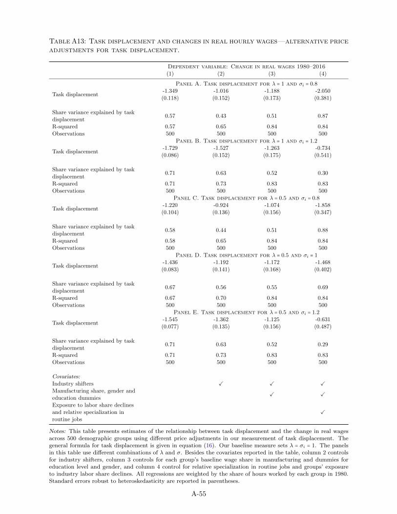
Table A13: Task displacement and changes in real hourly wages—alternative priceadjustments for task displacement.

Dependent variable: Change in real wages 1980–2016(1) (2) (3) (4)

Panel A. Task displacement for λ = 1 and σi = 0.8

Task displacement-1.349 -1.016 -1.188 -2.050(0.118) (0.152) (0.173) (0.381)

Share variance explained by taskdisplacement

0.57 0.43 0.51 0.87

R-squared 0.57 0.65 0.84 0.84Observations 500 500 500 500

Panel B. Task displacement for λ = 1 and σi = 1.2

Task displacement-1.729 -1.527 -1.263 -0.734(0.086) (0.152) (0.175) (0.541)

Share variance explained by taskdisplacement

0.71 0.63 0.52 0.30

R-squared 0.71 0.73 0.83 0.83Observations 500 500 500 500

Panel C. Task displacement for λ = 0.5 and σi = 0.8

Task displacement-1.220 -0.924 -1.074 -1.858(0.104) (0.136) (0.156) (0.347)

Share variance explained by taskdisplacement

0.58 0.44 0.51 0.88

R-squared 0.58 0.65 0.84 0.84Observations 500 500 500 500

Panel D. Task displacement for λ = 0.5 and σi = 1

Task displacement-1.436 -1.192 -1.172 -1.468(0.083) (0.141) (0.168) (0.402)

Share variance explained by taskdisplacement

0.67 0.56 0.55 0.69

R-squared 0.67 0.70 0.84 0.84Observations 500 500 500 500

Panel E. Task displacement for λ = 0.5 and σi = 1.2

Task displacement-1.545 -1.362 -1.125 -0.631(0.077) (0.135) (0.156) (0.487)

Share variance explained by taskdisplacement

0.71 0.63 0.52 0.29

R-squared 0.71 0.73 0.83 0.83Observations 500 500 500 500

Covariates:Industry shifters ✓ ✓ ✓

Manufacturing share, gender andeducation dummies

✓ ✓

Exposure to labor share declinesand relative specialization inroutine jobs

✓

Notes: This table presents estimates of the relationship between task displacement and the change in real wagesacross 500 demographic groups using different price adjustments in our measurement of task displacement. Thegeneral formula for task displacement is given in equation (16). Our baseline measure sets λ = σi = 1. The panelsin this table use different combinations of λ and σ. Besides the covariates reported in the table, column 2 controlsfor industry shifters, column 3 controls for each group’s baseline wage share in manufacturing and dummies foreducation level and gender, and column 4 control for relative specialization in routine jobs and groups’ exposureto industry labor share declines. All regressions are weighted by the share of hours worked by each group in 1980.Standard errors robust to heteroskedasticity are reported in parentheses.

A-55

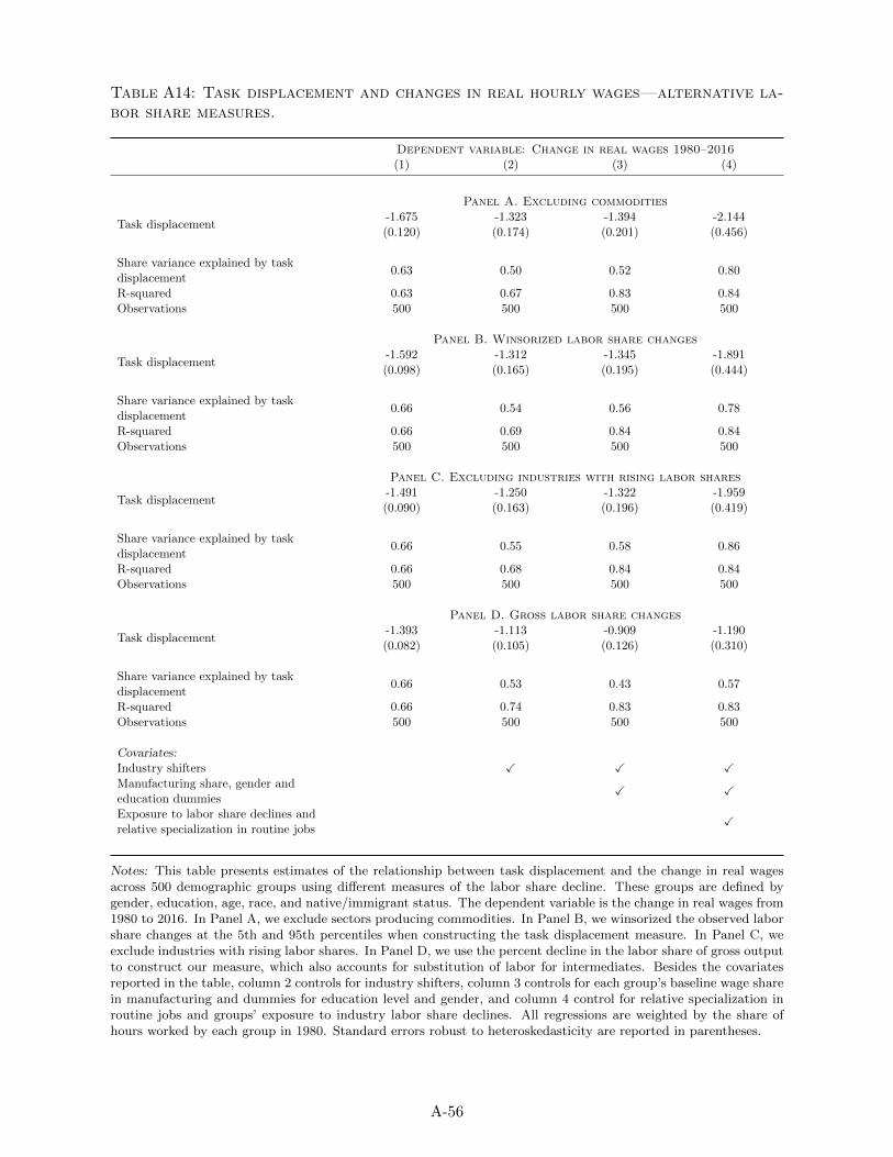
Table A14: Task displacement and changes in real hourly wages—alternative la-bor share measures.

Dependent variable: Change in real wages 1980–2016(1) (2) (3) (4)

Panel A. Excluding commodities

Task displacement-1.675 -1.323 -1.394 -2.144(0.120) (0.174) (0.201) (0.456)

Share variance explained by taskdisplacement

0.63 0.50 0.52 0.80

R-squared 0.63 0.67 0.83 0.84Observations 500 500 500 500

Panel B. Winsorized labor share changes

Task displacement-1.592 -1.312 -1.345 -1.891(0.098) (0.165) (0.195) (0.444)

Share variance explained by taskdisplacement

0.66 0.54 0.56 0.78

R-squared 0.66 0.69 0.84 0.84Observations 500 500 500 500

Panel C. Excluding industries with rising labor shares

Task displacement-1.491 -1.250 -1.322 -1.959(0.090) (0.163) (0.196) (0.419)

Share variance explained by taskdisplacement

0.66 0.55 0.58 0.86

R-squared 0.66 0.68 0.84 0.84Observations 500 500 500 500

Panel D. Gross labor share changes

Task displacement-1.393 -1.113 -0.909 -1.190(0.082) (0.105) (0.126) (0.310)

Share variance explained by taskdisplacement

0.66 0.53 0.43 0.57

R-squared 0.66 0.74 0.83 0.83Observations 500 500 500 500

Covariates:Industry shifters ✓ ✓ ✓

Manufacturing share, gender andeducation dummies

✓ ✓

Exposure to labor share declines andrelative specialization in routine jobs

✓

Notes: This table presents estimates of the relationship between task displacement and the change in real wagesacross 500 demographic groups using different measures of the labor share decline. These groups are defined bygender, education, age, race, and native/immigrant status. The dependent variable is the change in real wages from1980 to 2016. In Panel A, we exclude sectors producing commodities. In Panel B, we winsorized the observed laborshare changes at the 5th and 95th percentiles when constructing the task displacement measure. In Panel C, weexclude industries with rising labor shares. In Panel D, we use the percent decline in the labor share of gross outputto construct our measure, which also accounts for substitution of labor for intermediates. Besides the covariatesreported in the table, column 2 controls for industry shifters, column 3 controls for each group’s baseline wage sharein manufacturing and dummies for education level and gender, and column 4 control for relative specialization inroutine jobs and groups’ exposure to industry labor share declines. All regressions are weighted by the share ofhours worked by each group in 1980. Standard errors robust to heteroskedasticity are reported in parentheses.

A-56

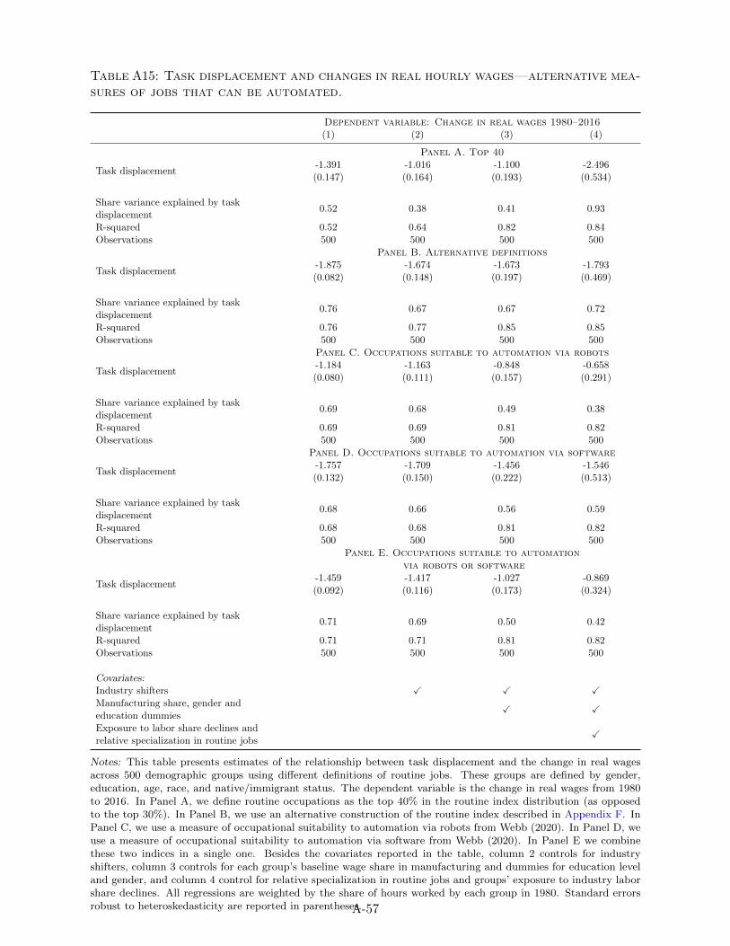
Table A15: Task displacement and changes in real hourly wages—alternative mea-sures of jobs that can be automated.

Dependent variable: Change in real wages 1980–2016(1) (2) (3) (4)

Panel A. Top 40

Task displacement-1.391 -1.016 -1.100 -2.496(0.147) (0.164) (0.193) (0.534)

Share variance explained by taskdisplacement

0.52 0.38 0.41 0.93

R-squared 0.52 0.64 0.82 0.84Observations 500 500 500 500

Panel B. Alternative definitions

Task displacement-1.875 -1.674 -1.673 -1.793(0.082) (0.148) (0.197) (0.469)

Share variance explained by taskdisplacement

0.76 0.67 0.67 0.72

R-squared 0.76 0.77 0.85 0.85Observations 500 500 500 500

Panel C. Occupations suitable to automation via robots

Task displacement-1.184 -1.163 -0.848 -0.658(0.080) (0.111) (0.157) (0.291)

Share variance explained by taskdisplacement

0.69 0.68 0.49 0.38

R-squared 0.69 0.69 0.81 0.82Observations 500 500 500 500

Panel D. Occupations suitable to automation via software

Task displacement-1.757 -1.709 -1.456 -1.546(0.132) (0.150) (0.222) (0.513)

Share variance explained by taskdisplacement

0.68 0.66 0.56 0.59

R-squared 0.68 0.68 0.81 0.82Observations 500 500 500 500

Panel E. Occupations suitable to automationvia robots or software

Task displacement-1.459 -1.417 -1.027 -0.869(0.092) (0.116) (0.173) (0.324)

Share variance explained by taskdisplacement

0.71 0.69 0.50 0.42

R-squared 0.71 0.71 0.81 0.82Observations 500 500 500 500

Covariates:Industry shifters ✓ ✓ ✓

Manufacturing share, gender andeducation dummies

✓ ✓

Exposure to labor share declines andrelative specialization in routine jobs

✓

Notes: This table presents estimates of the relationship between task displacement and the change in real wagesacross 500 demographic groups using different definitions of routine jobs. These groups are defined by gender,education, age, race, and native/immigrant status. The dependent variable is the change in real wages from 1980to 2016. In Panel A, we define routine occupations as the top 40% in the routine index distribution (as opposedto the top 30%). In Panel B, we use an alternative construction of the routine index described in Appendix F. InPanel C, we use a measure of occupational suitability to automation via robots from Webb (2020). In Panel D, weuse a measure of occupational suitability to automation via software from Webb (2020). In Panel E we combinethese two indices in a single one. Besides the covariates reported in the table, column 2 controls for industryshifters, column 3 controls for each group’s baseline wage share in manufacturing and dummies for education leveland gender, and column 4 control for relative specialization in routine jobs and groups’ exposure to industry laborshare declines. All regressions are weighted by the share of hours worked by each group in 1980. Standard errorsrobust to heteroskedasticity are reported in parentheses.A-57

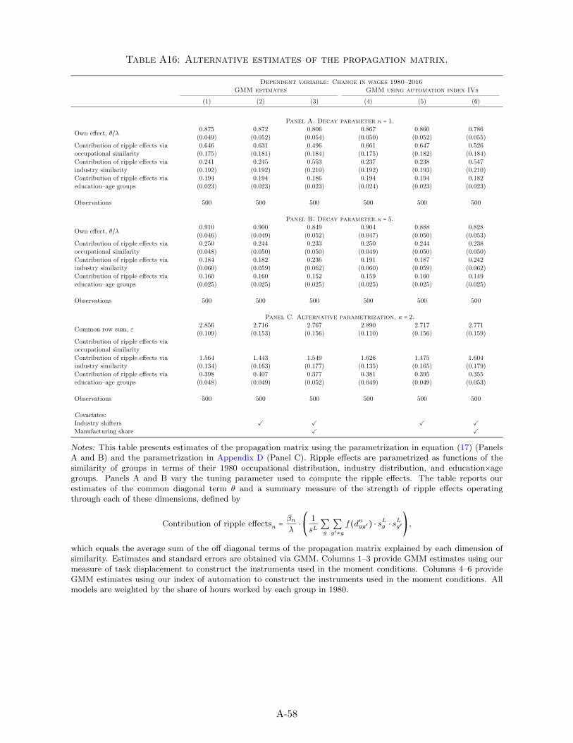
Table A16: Alternative estimates of the propagation matrix.

Dependent variable: Change in wages 1980–2016GMM estimates GMM using automation index IVs

(1) (2) (3) (4) (5) (6)

Panel A. Decay parameter κ = 1.

Own effect, θ/λ0.875 0.872 0.806 0.867 0.860 0.786

(0.049) (0.052) (0.054) (0.050) (0.052) (0.055)Contribution of ripple effects viaoccupational similarity

0.646 0.631 0.496 0.661 0.647 0.526(0.175) (0.181) (0.184) (0.175) (0.182) (0.184)

Contribution of ripple effects viaindustry similarity

0.241 0.245 0.553 0.237 0.238 0.547(0.192) (0.192) (0.210) (0.192) (0.193) (0.210)

Contribution of ripple effects viaeducation–age groups

0.194 0.194 0.186 0.194 0.194 0.182(0.023) (0.023) (0.023) (0.024) (0.023) (0.023)

Observations 500 500 500 500 500 500

Panel B. Decay parameter κ = 5.

Own effect, θ/λ0.910 0.900 0.849 0.904 0.888 0.828

(0.046) (0.049) (0.052) (0.047) (0.050) (0.053)Contribution of ripple effects viaoccupational similarity

0.250 0.244 0.233 0.250 0.244 0.238(0.048) (0.050) (0.050) (0.049) (0.050) (0.050)

Contribution of ripple effects viaindustry similarity

0.184 0.182 0.236 0.191 0.187 0.242(0.060) (0.059) (0.062) (0.060) (0.059) (0.062)

Contribution of ripple effects viaeducation–age groups

0.160 0.160 0.152 0.159 0.160 0.149(0.025) (0.025) (0.025) (0.025) (0.025) (0.025)

Observations 500 500 500 500 500 500

Panel C. Alternative parametrization, κ = 2.

Common row sum, ε2.856 2.716 2.767 2.890 2.717 2.771

(0.109) (0.153) (0.156) (0.110) (0.156) (0.159)Contribution of ripple effects viaoccupational similarity

Contribution of ripple effects viaindustry similarity

1.564 1.443 1.549 1.626 1.475 1.604(0.134) (0.163) (0.177) (0.135) (0.165) (0.179)

Contribution of ripple effects viaeducation–age groups

0.398 0.407 0.377 0.381 0.395 0.355(0.048) (0.049) (0.052) (0.049) (0.049) (0.053)

Observations 500 500 500 500 500 500

Covariates:Industry shifters ✓ ✓ ✓ ✓

Manufacturing share ✓ ✓

Notes: This table presents estimates of the propagation matrix using the parametrization in equation (17) (PanelsA and B) and the parametrization in Appendix D (Panel C). Ripple effects are parametrized as functions of thesimilarity of groups in terms of their 1980 occupational distribution, industry distribution, and education×agegroups. Panels A and B vary the tuning parameter used to compute the ripple effects. The table reports ourestimates of the common diagonal term θ and a summary measure of the strength of ripple effects operatingthrough each of these dimensions, defined by

Contribution of ripple effectsn =βnλ⋅⎛⎝

1

sL∑g

∑g′≠g

f(dngg′) ⋅ sLg ⋅ sLg′⎞⎠,

which equals the average sum of the off diagonal terms of the propagation matrix explained by each dimension ofsimilarity. Estimates and standard errors are obtained via GMM. Columns 1–3 provide GMM estimates using ourmeasure of task displacement to construct the instruments used in the moment conditions. Columns 4–6 provideGMM estimates using our index of automation to construct the instruments used in the moment conditions. Allmodels are weighted by the share of hours worked by each group in 1980.

A-58

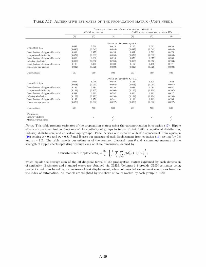
Table A17: Alternative estimates of the propagation matrix (Continued).

Dependent variable: Change in wages 1980–2016GMM estimates GMM using automation index IVs

(1) (2) (3) (4) (5) (6)

Panel A. Setting σi = 0.8.

Own effect, θ/λ0.682 0.668 0.615 0.706 0.692 0.639

(0.040) (0.042) (0.045) (0.042) (0.043) (0.046)Contribution of ripple effects viaoccupational similarity

0.509 0.477 0.426 0.537 0.519 0.475(0.079) (0.082) (0.084) (0.079) (0.083) (0.084)

Contribution of ripple effects viaindustry similarity

0.080 0.083 0.216 0.076 0.077 0.200(0.096) (0.096) (0.104) (0.096) (0.096) (0.104)

Contribution of ripple effects viaeducation–age groups

0.198 0.197 0.189 0.182 0.182 0.171(0.022) (0.022) (0.022) (0.022) (0.022) (0.022)

Observations 500 500 500 500 500 500

Panel B. Setting σi = 1.2.

Own effect, θ/λ1.045 1.038 0.949 1.121 1.125 1.022

(0.058) (0.061) (0.064) (0.061) (0.064) (0.067)Contribution of ripple effects viaoccupational similarity

0.195 0.184 0.130 0.081 0.084 0.057(0.104) (0.107) (0.106) (0.106) (0.108) (0.107)

Contribution of ripple effects viaindustry similarity

0.391 0.391 0.592 0.460 0.461 0.627(0.123) (0.123) (0.130) (0.124) (0.124) (0.130)

Contribution of ripple effects viaeducation–age groups

0.152 0.153 0.141 0.169 0.169 0.156(0.028) (0.028) (0.027) (0.028) (0.028) (0.027)

Observations 500 500 500 500 500 500

Covariates:Industry shifters ✓ ✓ ✓ ✓

Manufacturing share ✓ ✓

Notes: This table presents estimates of the propagation matrix using the parametrization in equation (17). Rippleeffects are parametrized as functions of the similarity of groups in terms of their 1980 occupational distribution,industry distribution, and education×age groups. Panel A uses our measure of task displacement from equation(16) setting λ = 0.5 and σi = 0.8. Panel B uses our measure of task displacement from equation (16) setting λ = 0.5and σi = 1.2. The table reports our estimates of the common diagonal term θ and a summary measure of thestrength of ripple effects operating through each of these dimensions, defined by

Contribution of ripple effectsn =βnλ⋅⎛⎝

1

sL∑g

∑g′≠g

f(dngg′) ⋅ sLg ⋅ sLg′⎞⎠,

which equals the average sum of the off diagonal terms of the propagation matrix explained by each dimensionof similarity. Estimates and standard errors are obtained via GMM. Columns 1-3 provide GMM estimates usingmoment conditions based on our measure of task displacement, while columns 4-6 use moment conditions based onthe index of automation. All models are weighted by the share of hours worked by each group in 1980.

A-59

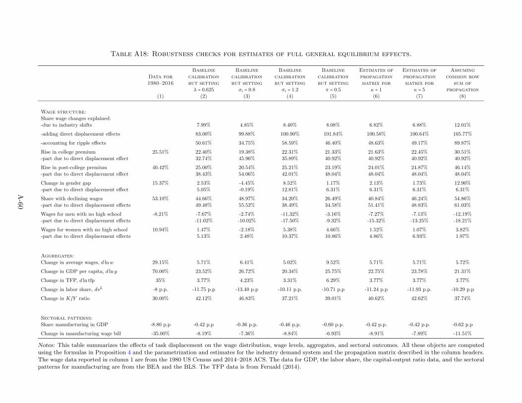
Table A18: Robustness checks for estimates of full general equilibrium effects.

Data for1980–2016

Baselinecalibrationbut settingλ = 0.625

Baselinecalibrationbut setting

σi = 0.8

Baselinecalibrationbut setting

σi = 1.2

Baselinecalibrationbut setting

π = 0.5

Estimates ofpropagationmatrix for

κ = 1

Estimates ofpropagationmatrix for

κ = 5

Assumingcommon row

sum ofpropagation

(1) (2) (3) (4) (5) (6) (7) (8)

Wage structure:Share wage changes explained:-due to industry shifts 7.99% 4.85% 8.40% 8.08% 6.82% 6.88% 12.01%

-adding direct displacement effects 83.00% 99.88% 100.90% 101.84% 100.58% 100.64% 105.77%

-accounting for ripple effects 50.61% 34.75% 58.59% 46.40% 48.63% 49.17% 89.87%

Rise in college premium 25.51% 22.40% 19.38% 22.31% 21.33% 21.63% 22.45% 30.51%-part due to direct displacement effect 32.74% 45.96% 35.89% 40.92% 40.92% 40.92% 40.92%

Rise in post-college premium 40.42% 25.00% 20.54% 25.21% 23.19% 24.01% 24.87% 46.14%-part due to direct displacement effect 38.43% 54.06% 42.01% 48.04% 48.04% 48.04% 48.04%

Change in gender gap 15.37% 2.53% -4.45% 8.52% 1.17% 2.13% 1.73% 12.90%-part due to direct displacement effect 5.05% -0.19% 12.81% 6.31% 6.31% 6.31% 6.31%

Share with declining wages 53.10% 44.66% 48.97% 34.20% 26.49% 40.84% 46.24% 54.86%-part due to direct displacement effects 49.48% 55.52% 38.49% 34.58% 51.41% 48.83% 61.03%

Wages for men with no high school -8.21% -7.67% -2.74% -11.32% -3.16% -7.27% -7.13% -12.19%-part due to direct displacement effects -11.02% -10.02% -17.50% -9.32% -15.32% -13.25% -18.21%

Wages for women with no high school 10.94% 1.47% -2.18% 5.38% 4.66% 1.52% 1.07% 3.82%-part due to direct displacement effects 5.13% 2.48% 10.37% 10.86% 4.86% 6.93% 1.97%

Aggregates:Change in average wages, d lnw 29.15% 5.71% 6.41% 5.02% 9.52% 5.71% 5.71% 5.72%

Change in GDP per capita, d ln y 70.00% 23.52% 26.72% 20.34% 25.75% 22.75% 23.78% 21.31%

Change in TFP, d ln tfp 35% 3.77% 4.23% 3.31% 6.29% 3.77% 3.77% 3.77%

Change in labor share, dsL -8 p.p. -11.75 p.p -13.40 p.p -10.11 p.p. -10.71 p.p -11.24 p.p -11.93 p.p. -10.29 p.p

Change in K/Y ratio 30.00% 42.12% 46.83% 37.21% 39.01% 40.62% 42.62% 37.74%

Sectoral patterns:Share manufacturing in GDP -8.80 p.p -0.42 p.p -0.36 p.p. -0.46 p.p. -0.60 p.p. -0.42 p.p. -0.42 p.p. -0.62 p.p

Change in manufacturing wage bill -35.00% -8.19% -7.36% -8.84% -6.93% -8.91% -7.89% -11.51%

Notes: This table summarizes the effects of task displacement on the wage distribution, wage levels, aggregates, and sectoral outcomes. All these objects are computedusing the formulas in Proposition 4 and the parametrization and estimates for the industry demand system and the propagation matrix described in the column headers.The wage data reported in column 1 are from the 1980 US Census and 2014–2018 ACS. The data for GDP, the labor share, the capital-output ratio data, and the sectoralpatterns for manufacturing are from the BEA and the BLS. The TFP data is from Fernald (2014).

A-60