Task Space Regions: A Framework for Pose-ConstrainedManipulation Planning

Dmitry Berenson1, Siddhartha Srinivasa2, and James Kuffner1

1The Robotics Institute, Carnegie Mellon University, Pittsburgh, PA, 15213, USA[dberenso, kuffner]@cs.cmu.edu

2Intel Labs Pittsburgh, Pittsburgh, PA, 15213, USAsiddhartha.srinivasa@intel.com

Abstract

We present a manipulation planning framework that allows robots to plan in the presence of constraints on end-effectorpose, as well as other common constraints. The framework has three main components: constraint representation, constraint-satisfaction strategies, and a general planning algorithm. These components come together to create an efficient andprobabilistically complete manipulation planning algorithm called the Constrained BiDirectional RRT (CBiRRT2). Theunderpinning of our framework for pose constraints is our Task Space Regions (TSRs) representation. TSRs are intuitiveto specify, can be efficiently sampled, and the distance to a TSR can be evaluated very quickly, making them ideal forsampling-based planning. Most importantly, TSRs are a general representation of pose constraints that can fully describemany practical tasks. For more complex tasks, such as those needed to manipulate articulated objects, TSRs can be chainedtogether to create more complex end-effector pose constraints. TSRs can also be intersected, a property that we use to rep-resent pose uncertainty. We provide a detailed description of our framework, prove probabilistic completeness for ourplanning approach, and describe several real-world example problems that illustrate the efficiency and versatility of theTSR framework.1

1 Introduction

Constraints involving the pose of a robot’s end-effector are some of the most common constraints in manipulation planning.They arise in tasks such as reaching to grasp an object, carrying a cup of coffee, or opening a door. Although ubiquitous,these constraints present significant challenges for planning algorithms. Because the allowed configurations of the robotare not known a priori, a planning algorithm must discover valid configurations as it plans. In the context of sampling-based motion planning, this exploration is done through sampling. Yet sampling pose constraints in an efficient andprobabilistically complete manner is difficult because they can produce lower-dimensional manifolds in the configurationspace of the robot. It is unclear how to represent such constraints in a general way, how to ensure that the exploration isefficient, and how to guarantee probabilistic completeness.

1This paper unifies and extends previous work appearing in [Berenson et al., 2009d, Berenson et al., 2009c, Berenson et al., 2009b,Berenson et al., 2009a, Berenson and Srinivasa, 2010].

1

Researchers have developed several algorithms capable of planning with end-effector pose constraints [Stilman, 2007,Koga et al., 1994, Yamane et al., 2004, Yao and Gupta, 2005, Drumwright and Ng-Thow-Hing, 2006, Bertram et al., 2006].Though often able to solve the problem at hand, these algorithms suffer from problems with efficiency [Stilman, 2007],probabilistic incompleteness [Koga et al., 1994, Yamane et al., 2004, Yao and Gupta, 2005], and overly-specialized con-straint representations [Drumwright and Ng-Thow-Hing, 2006, Bertram et al., 2006].

(a) (b) (c) (d)

Figure 1: The HERB and HRP3 robots executing paths planned using our pose-constrained manipulation planning framework.

We present a manipulation planning framework that allows robots to plan in the presence of pose constraints. The frame-work has three main components: an intuitive constraint representation, constraint-satisfaction strategies, and a generalplanning algorithm. These three components come together to create an efficient and probabilistically complete manipu-lation planning algorithm called the Constrained BiDirectional RRT (CBiRRT2). The underpinning of our framework forpose-related constraints is our Task Space Regions (TSRs) representation. TSRs are intuitive to specify, can be efficientlysampled, and the distance to a TSR can be evaluated very quickly, making them ideal for sampling-based planning. Mostimportantly, TSRs are a general representation of pose constraints that can describe many practical tasks. TSRs can alsobe chained to describe constraints on articulated objects and intersected to address pose uncertainty. CBiRRT2 exploresthe constraints of a given problem by sampling from TSRs and TSR Chains using projection methods and direct sam-pling of parameters. These samples are used to determine goals for the planner and to construct paths on the manifold ofconfigurations allowed by the constraints.

Our constrained manipulation planning framework also allows planning with multiple simultaneous constraints. For in-stance, collision, torque, and balance constraints can be included along with multiple constraints on end-effector pose.Closed-chain kinematics constraints can also be included as a relation between end-effector pose constraints without re-quiring specialized projection operators [Yakey et al., 2001] or sampling algorithms [Cortes and Simeon, 2004].

We have applied our framework to a wide range of problems for several robots (Figure 1), both in simulation and in thereal world. These problems include grasping in cluttered environments, lifting heavy objects, two-armed manipulation,and opening doors, to name a few. Despite this wide range of problems, our approach only requires three parameters, all ofwhich are constant across the examples described in this paper. We also provide a method for shortening paths generatedby our planner, an important component for producing practical paths with sampling-based planners. Finally, since we areoperating in the sampling-based planning paradigm, our constraint representations and constraint-satisfaction strategiescan be used by other planners such as Probabilistic Roadmaps (PRMs) [Kavraki et al., 1996].

In the following sections, we first discuss previous work related to our approach (Section 2). We then formulate the con-strained path planning problem and discuss three strategies for planning with constraints on configuration (Section 3).Section 4 presents TSRs, which can represent constraints on end-effector poses and goals. We then extend this representa-tion to handle more complex constraints by chaining TSRs together (Section 5). Section 6 describes the CBiRRT2 planner,which is capable of planning with TSRs and TSR Chains, among other constraints. Section 7 describes several exampleproblems and shows how to formulate constraints for these problems using TSRs. The performance of CBiRRT2 is also

2

evaluated on each example problem. We then describe an extension to the TSR framework that allows planning with objectpose uncertainty in Section 8. Finally, we provide a summary of the proof of probabilistic completeness for a class ofplanning algorithms which includes CBiRRT2 in Appendix A.

2 Background

Our framework builds on several developments in control theory and motion planning research. Some of the most success-ful methods in control theory for manipulation have come from local controllers that seek to minimize a given functionin the neighborhood of the robot’s current configuration through gradient-descent. For instance, controllers have beendeveloped for balancing two-legged robots [Sugihara and Nakamura, 2002], placing the end-effector somewhere in taskspace [Khatib, 1987], and collision-avoidance [Sentis and Khatib, 2005]. The technique of recursive null-space projec-tion [Sentis and Khatib, 2005] can satisfy multiple constraints simultaneously by prioritizing the constraints and satisfyinglower-priority constraints in the null-space of higher-priority ones. These controllers can succeed or fail depending on theprioritization of constraints and it is unclear which of the multiple simulatenous constraints should be prioritized ahead ofwhich others. Even if the prioritization issue is resolved, controllers based on gradient-descent only guarantee that a localminimum of the function is found, which may not be sufficient to solve the problem.

Researchers in control theory have also pursued more global solutions, such as building control policies through dynamicprogramming [Bellman, 1957]. However such approaches do not scale to the high-dimensional configuration spaces ofmost manipulators because of the exponential cost of computing optimal policies. Another popular approach has been tolearn policies from demonstration [Atkeson and Schaal, 1997, Bentivegna et al., 2004, Howard et al., 2008]. However, forour scope of manipulation problems, finding a set of examples that spans the space of tasks the manipulator is expected toperform as well as a robust way to generalize from these examples has proven quite difficult.

In motion planning, a number of efficient sampling-based planning algorithms have been developed for searching high-dimensional C-spaces [LaValle and Kuffner, 2000, Kavraki et al., 1996]. Sampling-based planners are designed to explorethe space of solutions efficiently, without the exhaustive computation required for dynamic programming and withoutbeing trapped by local minima like gradient-descent controllers. This global planning ability is acutely important formanipulation because even the most common constraints (like collision-avoidance) can trap approaches based on gradient-descent. Yet sampling-based planners falter when the constraints of a problem restrict the valid configurations to a lower-dimensional manifold in the C-space. It is unclear how to sample such manifolds efficiently and how to ensure probabilisticcompleteness.

Our strategy is to merge the best aspects of control theory and sampling-based planning to produce an algorithm thatsearches globally while satisfying constraints locally. The CBiRRT2 planner uses a bi-directional RRT to explore the con-straint manifold while enforcing constraints via rejection sampling and projection methods based on gradient-descent. Al-though CBiRRT2 is based on the Rapidly-exploring Random Tree (RRT) algorithm [LaValle and Kuffner, 2000], it is possi-ble to adapt some of the ideas and techniques in this paper to other search algorithms such as the PRM [Kavraki et al., 1996].We selected RRTs for their ability to explore C-space while retaining an element of “greediness” in their search for a so-lution. The greedy element is most evident in the bidirectional version of the RRT algorithm (BiRRT), where two trees,one grown from the start configuration and one grown from the goal configuration, take turns exploring the space andattempting to connect to each other. In this paper, we demonstrate that such a search strategy is also effective for motionplanning problems involving pose constraints when it is coupled with the proper strategies for handling those constraints.

The task of the CBiRRT2 planner is to construct a C-space path that lies on the constraint manifolds induced by poseconstraints (as well as constraints like collision-avoidance, balance, and torque). We distinguish this task from the taskof tracking pre-scripted end-effector paths [Seereeram and Wen, 1995, Oriolo et al., 2002, Oriolo and Mongillo, 2005] be-cause we do not assume an end-effector path is given. CBiRRT2 uses gradient-descent inverse-kinematics techniques[Sentis and Khatib, 2005, Sciavicco and Siciliano, 2000] to meet pose constraints and sample goal configurations. The al-gorithm plans in the full C-space of the robot, which implicitly allows it to search the null-space of pose constraints, unlike

3

task-space planners [Koga et al., 1994, Yamane et al., 2004, Yao and Gupta, 2005], which assign a single configuration toeach task-space point (from a potentially infinite number of possible configurations). Exploration of the null-space isnecessary for probabilistic completeness and can be useful for satisfying other constraints, such as avoiding obstacles ormaintaining balance, though our constraint representation could be incorporated into task-space planners as well.

Algorithms similar to CBiRRT2 have been proposed by [Yakey et al., 2001] and [Stilman, 2007].[Yakey et al., 2001] pro-posed using Randomized Gradient Descent (RGD) to meet closed-chain kinematics constraints. RGD uses random-sampling of the C-space to iteratively project a sample towards an arbitrary constraint [Yao and Gupta, 2005]. Though[Yakey et al., 2001] showed how to incorporate RGD into a sampling-based planner and their method is quite general, itrequires significant parameter-tuning and they dealt only with closed-chain kinematic constraints, which are a special caseof the pose constraints used in this paper. Furthermore, [Stilman, 2007] showed that when RGD is extended to work withmore general pose constraints it is significantly less efficient than Jacobian pseudo-inverse projection and it is sometimesunable to meet more stringent constraints. Our approach is similar to [Stilman, 2007] in that we use an RRT-based plannerwith Jacobian pseudo-inverse projection, however we differ in the specifics of the planning algorithm and use TSRs, whichare a more general constraint representation.

Another key feature of CBiRRT2 is that it can sample TSRs to produce goal configurations. Other researchers haveapproached the problem of ambiguous goal specification by sampling some number of goals before running the planner[Stilman et al., 2007, Hirano et al., 2005], which limits the planner to a small set of solutions from a region which is reallycontinuous. Another approach is to bias a single-tree planner toward the goal regions, however this approach usuallyconsiders single points [Drumwright and Ng-Thow-Hing, 2006, Vande Weghe et al., 2007] in the task space or is hand-tuned for specific goal regions [Bertram et al., 2006].

3 Constraints on Configuration

Depending on the robot and the task, many types of constraints can limit a robot’s motion. This paper focuses on scle-ronomic holonomic constraints, which are time-invariant constraints evaluated at a given configuration of the robot. Letthe configuration space of the robot be Q. A path in that space is defined by τ : [0, 1] → Q. We consider constraintsevaluated as a function of a configuration q ∈ Q in τ . The location of q in τ determines which constraints are active atthat configuration. Thus a constraint is defined as the pair {C(q), s}, where C(q) ∈ R ≥ 0 is the constraint-evaluationfunction. C(q) determines whether the constraint is met at that q and s ⊆ [0, 1] is the domain of this constraint, i.e. wherein the path τ the constraint is active. To say that a given constraint is satisfied we require that C(q) = 0 ∀q ∈ τ(s). Eachconstraint defined in this way implicitly defines a manifold in Q where τ(s) is allowed to exist. Given a constraint, themanifold of configurations that meet this constraintMC ⊆ Q is defined as

MC = {q ∈ Q : C(q) = 0} (1)

In order for τ to satisfy a constraint, all the elements of τ(s) must lie withinMC . If ∃q /∈MC for q ∈ τ(s) then τ is saidto violate the constraint.

In general, we can define any number of constraints for a given task, each with their own domain. Let a set of n constraint-evaluation functions be C and the set of domains corresponding to those functions be S. Then we define the constrainedpath planning problem as:

find τ : q ∈MCi ∀q ∈ τ(Si)∀i ∈ {1...n} (2)

4

(a) (b)

Figure 2: (a) Pose constraint for a 3-link manipulator: The end-effector must be on the line with an orientation within ±0.7rad ofdownward. (b) The manifold induced by this constraint in the C-space of this robot.

Note that the domains of two or more constraints may overlap in which case an element of τ may need to lie within two ormore constraint manifolds.

3.1 Difficulties of Constrained Path Planning

Two main issues make solving the constrained path planning problem difficult. First, constraint manifolds are difficult torepresent. There is no known analytical representation for many types of constraint manifolds (including pose constraints)and the high dimensional C-spaces of most practical robots make representing the manifold through exhaustive samplingprohibitively expensive. It is possible to parameterize some constraint manifolds, however this can be insufficient forplanning paths because the mapping from the parameter space to the manifold can be nonsmooth (see Figure 2). Thus,although we can construct a smooth path in the parameter space, its image on the constraint manifold may be disjoint.Restrictions imposed on the mapping to render it smooth, like imposing a one-to-one mapping from pose to configuration,compromise on completeness.

Second, and acutely important for pose constraints, is the fact that constraint manifolds can be of a lower dimension thanthe ambient C-space. Lower-dimensional manifolds cannot be sampled using rejection sampling (the sampling techniqueused by most sampling-based planners) and thus more sophisticated sampling techniques are required. A key challenge isto demonstrate that the distribution of samples produced by these techniques densely covers the constraint manifold, whichis necessary for probabilistic completeness.

We address the first issue by using a sampling-based planner that explores the constraint manifold in the C-space (not in theparameter space). This planner uses a variety of sampling techniques to generate samples on constraint manifolds (Section3.2). One of these techniques is able to sample lower-dimensional constraint manifolds and we validate the probabilisticcompleteness of this approach in Appendix A, thus addressing the second issue.

3.2 Sampling on Constraint Manifolds

In order to solve the constrained path planning problem, a sampling-based planning algorithm must be able to generateconfigurations that lie on constraint manifolds. We describe three general strategies for generating these configurations:rejection, projection, and direct sampling (see Figure 3).

In the rejection strategy, we simply generate a sample q ∈ Q and check if C(q) = 0, if this is not the case, we deem qinvalid. This strategy is effective when there is a high probability of randomly sampling configurations that satisfy this

5

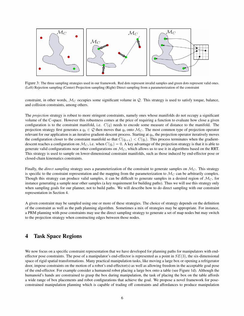
Figure 3: The three sampling strategies used in our framework. Red dots represent invalid samples and green dots represent valid ones.(Left) Rejection sampling (Center) Projection sampling (Right) Direct sampling from a parameterization of the constraint

constraint, in other words, MC occupies some significant volume in Q. This strategy is used to satisfy torque, balance,and collision constraints, among others.

The projection strategy is robust to more stringent constraints, namely ones whose manifolds do not occupy a significantvolume of the C-space. However this robustness comes at the price of requiring a function to evaluate how close a givenconfiguration is to the constraint manifold, i.e. C(q) needs to encode some measure of distance to the manifold. Theprojection strategy first generates a q0 ∈ Q then moves that q0 ontoMC . The most common type of projection operatorrelevant for our application is an iterative gradient-descent process. Starting at q0, the projection operator iteratively movesthe configuration closer to the constraint manifold so that C(qi+1) < C(qi). This process terminates when the gradient-descent reaches a configuration onMC , i.e. when C(qi) = 0. A key advantage of the projection strategy is that it is able togenerate valid configurations near other configurations onMC , which allows us to use it in algorithms based on the RRT.This strategy is used to sample on lower-dimensional constraint manifolds, such as those induced by end-effector pose orclosed-chain kinematics constraints.

Finally, the direct sampling strategy uses a parameterization of the constraint to generate samples onMC . This strategyis specific to the constraint representation and the mapping from the parameterization toMC can be arbitrarily complex.Though this strategy can produce valid samples, it can be difficult to generate samples in a desired region of MC , forinstance generating a sample near other samples (a key requirement for building paths). Thus we will use this strategy onlywhen sampling goals for our planner, not to build paths. We will describe how to do direct sampling with our constraintrepresentation in Section 4.

A given constraint may be sampled using one or more of these strategies. The choice of strategy depends on the definitionof the constraint as well as the path planning algorithm. Sometimes a mix of strategies may be appropriate. For instance,a PRM planning with pose constraints may use the direct sampling strategy to generate a set of map nodes but may switchto the projection strategy when constructing edges between those nodes.

4 Task Space Regions

We now focus on a specific constraint representation that we have developed for planning paths for manipulators with end-effector pose constraints. The pose of a manipulator’s end-effector is represented as a point in SE(3), the six-dimensionalspace of rigid spatial transformations. Many practical manipulation tasks, like moving a large box or opening a refrigeratordoor, impose constraints on the motion of a robot’s end-effector(s) as well as allowing freedom in the acceptable goal poseof the end-effector. For example consider a humanoid robot placing a large box onto a table (see Figure 1d). Although thehumanoid’s hands are constrained to grasp the box during manipulation, the task of placing the box on the table affordsa wide range of box placements and robot configurations that achieve the goal. We propose a novel framework for pose-constrained manipulation planning which is capable of trading off constraints and affordances to produce manipulation

6

plans for high degree of freedom robots, like humanoids or mobile manipulators.

Our constrained manipulation planning framework uses a novel unifying representation of constraints and affordanceswhich we term Task Space Regions (TSRs). TSRs describe end-effector constraint sets as subsets of SE(3). These subsetsare particularly useful for specifying manipulation tasks ranging from reaching to grasp an object and placing it on a surfaceor in a volume, to manipulating objects with constraints on their pose such as transporting a glass of water without spillingor sliding a milk jug on a table.

TSRs are specifically designed to be used with sampling-based planners. As such, it is straightforward to specify TSRs forcommon tasks, to compute distance from a given pose to a TSR (necessary for the projection strategy), and to sample froma TSR using direct sampling. Furthermore, multiple TSRs can be defined for a given task, which allows the specificationof multiple simultaneous constraints and affordances.

TSRs are not intended to capture every conceivable constraint on pose. Instead they are meant to be simple descriptionsof common manipulation tasks that are useful for planning. We have also developed a more complex representation forarticulated constraints called TSR Chains, which is discussed in Section 5. Finally, we discuss the limitations of theserepresentations in Section 9.

4.1 TSR Definition

Throughout this section, we will be using transformation matrices of the form Tab , which specifies the pose of b in the

coordinates of frame a. Tab , written in homogeneous coordinates, consists of a 3 × 3 rotation matrix Ra

b and a 3 × 1translation vector tab .

Tab =

[Ra

b tab0 1

](3)

A TSR consists of three parts:

• T0w: transform from the origin to the TSR frame w

• Twe : end-effector offset transform in the coordinates of w

• Bw: 6× 2 matrix of bounds in the coordinates of w:

Bw =

xmin xmax

ymin ymax

zmin zmax

ψmin ψmax

θmin θmax

φmin φmax

(4)

The first three rows of Bw bound the allowable translation along the x, y, and z axes (in meters) and the last three boundthe allowable rotation about those axes (in radians), all in the w frame. Note that this assumes the Roll-Pitch-Yaw (RPY)Euler angle convention, which is used because it allows bounds on rotation to be intuitively specified.

In practice, the w frame is usually centered at the origin of an object held by the hand or at a location on an object thatis useful for grasping. We use an end-effector offset transform Tw

e , because we do not assume that w directly encodes

7

the pose of the end-effector. Twe allows the user to specify an offset from w to the origin of the end-effector e, which is

extremely useful when we wish to specify a TSR for an object held by the hand or a grasping location which is offset frome; for instance in between the fingers. For some example Tw

e transforms, see Figure 4 and Figure 5.

4.2 Distance to TSRs

When using the projection strategy with TSRs, it will be necessary to find the distance from a given configuration qsto a TSR (please follow the explanation below in Figure 5). Because we do not have an analytical representation of theconstraint manifold corresponding to a TSR, we compute this distance in task space. Given a qs, we use forward kinematicsto get the position of the end-effector at this configuration T0

s. We then apply the inverse of the offset Twe to get T0

s′ , whichis the pose of the grasp location or the pose of the object held by the hand in world coordinates.

T0s′ = T0

s(Twe )−1 (5)

We then convert this pose from world coordinates to the coordinates of w.

Tws′ = (T0

w)−1T0s′ (6)

Now we convert the transform Tws′ into a 6 × 1 displacement vector from the origin of the w frame. This displacement

represents rotation in the RPY convention so it is consistent with the definition of Bw.

dw =

tws′

arctan 2(Rws′32,Rw

s′33)

− arcsin(Rws′31

)

arctan 2(Rws′21,Rw

s′11)

(7)

Taking into account the bounds of Bw, we get the 6× 1 displacement vector to the TSR ∆x

∆xi =

dwi − Bw

i,1 if dwi < Bwi,1

dwi − Bwi,2 if dwi > Bw

i,2

0 otherwise(8)

Figure 4: The w and e frames used to define end-effector goal TSRs for a soda can and a pitcher.

8

Figure 5: Transforms and coordinate frames involved in computing the distance to TSRs. The robot is in a sample configuration whichhas end-effector transform s and the hand near the soda can at transform e represents the Tw

e defined by the TSR.

where i indexes through the six rows of Bw and six elements of ∆x and dw. ‖∆x‖ is the distance to the TSR. Notethat we implicitly weigh rotation in radians and translation in meters equally when computing ‖∆x‖ but the two typesof units can be weighed in an arbitrary way to produce a distance metric that considers one or the other more important.Because of the inherent redundancy of the RPY Euler angle representation, there are several sets of angles that representthe same rotation. To find the minimal distance by our metric, we evaluate the norm of each of the possible RPY anglesets capable of yielding the minimum displacement. This set consists of the {∆x4,∆x5,∆x6} defined above as well as theeight equivalent rotations {∆x4 ± π,−∆x5 ± π,∆x6 ± π}.

If we define multiple TSRs for a given manipulator, we extend our distance computation to evaluate distance to all relevantTSRs and return the smallest.

4.3 Direct Sampling of TSRs

When using TSRs to specify goal end-effector poses, it will be necessary to draw sample poses from TSRs. Sampling froma single TSR is done by first sampling a random value between each of the bounds defined by Bw with uniform probability.These values are then compiled in a displacement dwsample and converted into the transformation Tw

sample. We can thenconvert this sample into world coordinates after applying the end-effector transformation.

T0sample′ = T0

wTwsampleTw

e (9)

We observe that while our method ensures a uniform sampling in the bounds of Bw, it could produce a biased sampling inthe subspace of constrained spatial displacements SE(3) that Bw parameterizes. However this bias has not had a significantimpact on the runtime or success-rate of our algorithms.

In the case of multiple TSRs specified for a single task, we must first decide which TSR to sample from. If the bounds ofall TSRs enclose six-dimensional volumes, we can choose among TSRs in proportion to their volume. However a volume-

9

proportional sampling will ignore TSRs that encompass volumes of less than six dimensions because they have no volumein the six-dimensional space. To address this issue we use a weighted sampling scheme that samples TSRs proportional tothe sum of the differences between their bounds.

ζi =

6∑j=1

(Bwij,2 − Bwi

j,1

)(10)

where ζi and Bwi are the weight and bounds of the ith TSR, respectively. Sampling proportional to ζi allows us to samplefrom TSRs of any dimension except 0 while giving preference to TSRs that encompass more volume. TSRs of dimension0, i.e. points, are given a fixed probability of being sampled. In general, any sampling scheme for selecting a TSR can beused as long as there is a non-zero probability of selecting any TSR.

4.4 Planning with TSRs as Goal Sets

TSRs can be used to sample goal end-effector placements of a manipulator, as would be necessary in a grasping or object-placement task. The constraint for using TSRs in this way is:

{C(q) = DistanceToTSR(q), s = [1]} (11)

Where the DistanceToTSR function implements the method of Section 4.2 and s refers to the domain of the constraint(Section 3).

To generate valid configurations in theMC corresponding to this constraint, we can use direct sampling of TSRs (Section4.3) and pass the sampled pose to an IK solver to generate a valid configuration. In order to ensure that we don’t excludeany part of the constraint manifold, the IK solver used should not exclude any configurations from consideration. This canbe achieved using an analytical IK solver for manipulators with six or fewer DOF. For manipulators with more than sixDOF, we can use a pseudo-analytical IK solver, which discretizes or samples all but six joints.

Alternatively, we can use the projection strategy to sample the manifold. This would take the form of an iterative IK solver,which starts at some initial configuration. This configuration should be randomized to ensure exploration of the constraintmanifold. Note that this strategy is prone to local minima and can be relatively slow to compute, so we use it only whenan analytical or pseudo-analytical IK solver is not available (for instance with a humanoid).

Of course the same definition and strategies apply to sampling starting configurations as well as goal configurations.

4.5 Planning with TSRs as Pose Constraints

TSRs can also be used for planning with constraints on end-effector pose for the entire path. The constraint definition forsuch a use of TSRs differs from Equation 11 in the domain of the constraint:

{C(q) = DistanceToTSR(q), s = [0, 1]} (12)

Since the domain of this constraint spans the entire path, the planning algorithm must ensure that each configuration it

10

Algorithm 1: J+Projection(q)

while true do1

∆x← DisplacementFromTSR(q);2

if ‖∆x‖ < ε then3

return q;4

end5

J← GetJacobian(q);6

∆qerror ← JT (JJT )−1∆x;7

q← (q −∆qerror);8

end9

deems valid lies within the constraint manifold. While the rejection strategy can be used to generate valid configurationsfor TSRs whose bounds encompass a six-dimensional volume, the projection strategy can be used for all TSRs.

One method of projection for TSRs is shown in Algorithm 1. This method uses the Jacobian pseudo-inverse (J+)[Sciavicco and Siciliano, 2000] to iteratively move a given configuration to the constraint manifold defined by a TSR.

The DisplacementFromTSR function returns the displacement from q to a TSR, i.e. the result of Equation 8. The GetJaco-bian function computes the Jacobian of the manipulator at q. Though Algorithm 1 describes the projection conceptually,in practice we must also take into account the issues of step-size, singularity avoidance, and joint limits when projectingconfigurations. We will show, in Appendix A, that the distribution of samples generated on the constraint manifold by thisprojection operator covers the manifold, which is a necessary property for probabilistic completeness.

It is important to note that we can also use the method of Section 4.3 to generate samples directly from TSRs and thencompute IK to obtain configurations that place the end-effector at those samples. Such a strategy would be especiallyuseful when planning in task space, i.e. the parameter space of pose constraints, instead of C-space because it would allowthe task space to be explored while providing configurations for each task-space point (similar to [Yao and Gupta, 2005]).However, we prefer the completeness properties of C-space planners, so we focus on those in this paper.

5 Task Space Region Chains

While we showed that TSRs are intuitive to specify, can be quickly sampled, and the distance to TSRs can be evaluatedefficiently, a single TSR, or even a finite set of TSRs, is sometimes insufficient to capture the pose constraints of a giventask. To describe more complex constraints such as closed-chain kinematics and manipulating articulated objects, thissection introduces the concept of TSR Chains, which are defined by linking a series of TSRs. Though direct sampling ofTSR Chains follows clearly from that of TSRs, the distance metric for TSR Chains is extremely different.

To motivate the need for a more complex representation consider the task of opening a door while allowing the end-effectorto rotate about the door handle (see Figure 6). It is straightforward to specify the rotation of the door about its hinge as asingle TSR and to specify the rotation of the end-effector about the door’s handle as a single TSR if the door’s position isfixed. However, the product of these two constraints (allowing the end-effector to rotate about the handle while the door ismoving) cannot be completely specified with a finite set of TSRs. In order to allow more complex constraint representationsin the TSR framework, we present TSR Chains, which are constructed by linking a series of TSRs.

11

Figure 6: The virtual manipulator for the door example. The green dotted lines represent the links of the virtual manipulator and thered dot and arrow represent the virtual end-effector, which is at transform T0

vee.

5.1 TSR Chain Definition

A TSR chain C = {C1,C2, ...,Cn} consists of a set of n TSRs with the following additional property:

Ci.T0w = (Ci−1.T0

w)(Ci−1.Twsample)(Ci−1.Tw

e ) (13)

for i = {2...n} where Ci corresponds to the ith TSR in the chain and Ci.{·} refers to an element of the ith TSR. Of coursea TSR Chain can consist of only one TSR, in which case it is identical to a normal TSR. Ci.Tw

sample can be any transformobtained by sampling from inside the bounds of Ci.Bw. Thus we do not know Ci.T0

w until we have determined Twsample

values for all previous TSRs in the chain. By coupling TSRs in this way the TSR Chain structure can represent constraintsthat would otherwise require an infinite number of TSRs to specify.

A TSR chain can also be thought of as a virtual serial-chain manipulator. Again consider the door example. To define theTSR chain for this example, we can imagine a virtual manipulator that is rooted at the door’s hinge. The first link of thevirtual manipulator rotates about the hinge and extends from the hinge to the handle. At the handle, we define another linkthat rotates about the handle and extends to where a robot’s end-effector would be if the robot were grasping the handle(see Figure 6). C1.Tw

sample would be a rotation about the door’s hinge corresponding to how much the door had beenopened. In this way, we could see the Tw

sample values for each TSR as transforms induced by the “joint angles” of thevirtual manipulator. The joint limits of these virtual joints are defined by the values in Bw.

5.2 Direct Sampling From TSR Chains

To directly sample a TSR Chain we first sample from within C1.Bw to obtain C1.Twsample. This is done by sampling

uniformly between the bounds in Bw, compiling the sampled values into a displacement dwsample = [x y z ψ θ φ] andconverting that displacement to the transform C1.Tw

sample. We then use this sample to determine C2.T0w via Equation 13.

We repeat this process for each TSR in the chain until we reach the nth TSR. We then obtain a sample in the world frame:

12

(a) (b) (c)

Figure 7: Depiction of the IK handshaking procedure. (a) The virtual manipulator starts in some configuration. (b) Finding the closestconfiguration of the virtual manipulator. (c) The robot’s manipulator moves to meet the constraint.

T0sample′ = (Cn.T0

w)(Cn.Twsample)(Cn.Tw

e ) (14)

Note that the sampling of TSR chains in this way is biased but the sampling will cover the entire set. To see this, imaginea virtual manipulator with many links. It can be readily seen that many sets of different joint values (essentially Tw

sample

values) of the virtual manipulator will map to the same end-effector transform. However, if the virtual manipulator’s end-effector is at the boundary of the virtual manipulator’s reachability, only one set of joint values maps to the end-effectorpose (when the manipulator is fully outstretched). Thus some T0

sample′ values can have a higher chance of being sampledthan others, depending on the definition of the TSR Chain. Clearly a uniform sampling would be ideal but we have foundthat this biased sampling is sufficient for the practical tasks we consider.

If there is more than one TSR Chain defined for a single manipulator, this means that we have the option of drawing asample from any of these TSR Chains. We choose a TSR Chain for sampling with probability proportional to the sum ofthe differences between the bounds of all TSRs in that chain.

5.3 Distance to TSR Chains

Though the sampling method for TSR Chains follows directly from the sampling method for TSRs, evaluating distance toa TSR Chain is fundamentally different from evaluating distance to a TSR. This is because we do not know which Tw

sample

values for each TSR in the chain yield the minimum distance to a query transform T0s (derived from a query configuration

qs using forward kinematics).

To approach this problem, it is again useful to think of the TSR chain as a virtual manipulator (See Figure 7a). Findingthe correct Tw

sample values for each TSR is equivalent to finding the joint angles of the virtual manipulator that bring itsvirtual end-effector as close to T0

s as possible. Thus we can see this distance-checking problem as a form of the standardIK problem, which is to find the set of joint angles that places an end-effector at a given transform. Depending on theTSR Chain definition and T0

s, the virtual manipulator may not be able to reach the desired transform, in which case wewant the virtual end-effector to get as close as possible. Thus we can apply standard iterative IK techniques based on theJacobian pseudo-inverse to move the virtual end-effector to a transform that is as close as possible to T0

s (see Figure 7b).Once we obtain the joint angles of the virtual manipulator, we convert them to Tw

sample values and forward-chain to obtainthe virtual end-effector position T0

vee. We then convert T0s to the virtual end-effector’s frame:

Tvees = (T0

vee)−1T0

s (15)

13

and then convert to the displacement form:

dvees =

tvees

arctan 2(Rvees32 ,R

vees33 )

− arcsin(Rvees31 )

arctan 2(Rvees21 ,R

vees11 )

(16)

‖dvees ‖ is the distance between T0s and T0

vee.

Once the distance is evaluated we can employ the projection strategy by calling the IK algorithm for the robot’s manipulatorto move the robot’s end-effector to T0

vee to meet the constraint specified by this TSR Chain (Figure 7c). We term thisprocess of calling IK for the virtual manipulator and the robot in sequence IK handshaking.

Just as with TSR Chains used for sampling, we may define more than one TSR Chain as a constraint for a single manipu-lator. This means that we have the option of satisfying any of these TSR Chains to produce a valid configuration. To findwhich chain to satisfy, we perform the distance check from our current configuration to each chain and choose the one thathas the smallest distance.

5.4 Physical Constraints

In the door example, the first TSR corresponds to a physical joint of a body in the environment but the second one ispurely virtual; i.e. defining a relation between two frames that is not enforced by a joint in the environment (in thiscase the relation is between the robot’s end-effector and the handle of the door). It is important to note that TSR Chainsinherently accommodate such mixing of real and virtual constraints. In fact a TSR Chain can consist of purely virtualor purely physical constraints. However, when planning with TSR Chains, special care must be taken to ensure that anyphysical joints (such as the door’s hinge) be synchronized with their TSR Chain counterparts. This is done by includingthe configuration of any physical joints corresponding to elements of TSR Chains in the configuration space searched bythe planner (see Section 6.3).

In the case that the physical constraints included in the TSR Chain form a redundant manipulator, the inverse-kinematicsalgorithm for the TSR Chain should be modified to account for the physical properties of the chain. For instance, if thechain is completely passive, a term that that minimizes the potential energy of the chain should be applied in the null-spaceof the Jacobian pseudo-inverse to find a local minimum-energy configuration of the chain. In general, chains can havevarious physical properties that may not be easy to account for using an IK solver. In that case, we recommend a physicalsimulation of the movement of the end-effector from it’s initial pose to T0

vee as it is being pulled by the robot to find theresting configuration of the chain.

5.5 Notes on Implementation

Whenever we create a TSR Chain, we also create its virtual manipulator in simulation so that we can perform IK on thismanipulator and get the location of the virtual end-effector. When we refer to the joint values of a TSR Chain, we areactually referring to the joint values of that TSR Chain’s virtual manipulator. Also, to differentiate whether a TSR Chainshould be used for sampling goals or constraining configurations or both, we specify how the chain should be used in itsdefinition. When inputing TSR Chains into our planner, we specify which manipulator of the robot they correspond to aswell as any physical DOFs that correspond to elements of the chain.

14

6 The CBiRRT2 Algorithm

This section describes the Constrained BiDirectional RRT (CBiRRT2) planner, which is capable of planning with TSRChains among other constraints. Since the representation of TSR chains subsumes that of TSRs, the planner can incorporatethe uses of TSRs already described. In this section we describe the operations of the planner. Several example problemsas well as CBiRRT2’s performance on these problems are shown in Section 7. We prove the probabilistic completeness ofCBiRRT2 when planning with pose constraints in Appendix A.

6.1 Planner Operation

CBiRRT2 takes into account constraints on the configuration of the robot during its path as well as constraints on the goalconfiguration of the robot. Constraints on the poses and goal locations of the robot’s end-effectors are specified as TSRChains.

Algorithm 2: CBiRRT2(Qs, Qg)

Ta.Init(Qs); Tb.Init(Qg);1

while TimeRemaining() do2

Tgoal = GetBackwardTree(Ta, Tb);3

if size(Tgoal) = 0 or rand(0, 1) < Psample then4

AddRoot(Tgoal);5

else6

qrand← RandomConfig();7

qanear ← NearestNeighbor(Ta, qrand);8

qareach← ConstrainedExtend(Ta, qanear, qrand);9

qbnear ← NearestNeighbor(Tb, qareached);10

qbreach← ConstrainedExtend(Tb, qbnear, qareach);11

if qareach = qbreach then12

P ← ExtractPath(Ta, qareach, Tb, qbreach);13

return ShortenPath(P );14

else15

Swap(Ta, Tb);16

end17

end18

end19

return ∅;20

Algorithm 3: ConstrainedExtend(T , qnear, qtarget)

qs← qnear; qolds ← qnear;1

while true do2

if qtarget = qs then3

return qs;4

else if ‖qtarget − qs‖ > ‖qolds − qtarget‖ then5

return qolds ;6

end7

qolds ← qs;8

qs← qs + min(∆qstep, ‖qtarget − qs‖) (qtarget−qs)‖qtarget−qs‖ ;9

c← GetConstraintValues(T , qolds );10

{qs, c} ← ConstrainConfig(qolds , qs, c,∅);11

if qs 6= ∅ then12

T .AddVertex(qs, c);13

T .AddEdge(qolds , qs);14

else15

return qolds ;16

end17

end18

CBiRRT2 operates by growing two trees in the C-space of the robot (please follow the explanation below in Algorithm 2).At each iteration, CBiRRT2 chooses between one of two modes: exploration of the C-space using the two trees or directsampling from a set of TSR Chains. The probability of choosing to sample is defined by the parameter Psample.

If the algorithm chooses to sample, it calls the AddRoot function, which tries to inject a goal configuration into thebackward tree Tgoal. If the algorithm chooses to explore the C-space, one of the trees grows a branch toward a randomly-sampled configuration qrand using the ConstrainedExtend function. The branch grows as far as possible toward qrand butmay be stalled due to collision or constraint violation and will terminate at qareach. The other tree then grows a branchtoward qareach, again growing as far as possible toward this configuration. If the other tree reaches qareach, the trees haveconnected and a path has been found. If not, the trees are swapped and the above process is repeated.

The ConstrainedExtend function (see Algorithm 3) iteratively moves from a configuration qnear toward a configuration

15

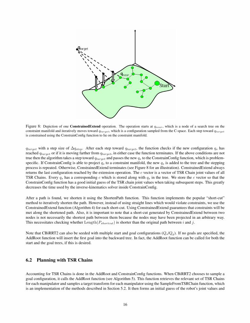
Figure 8: Depiction of one ConstrainedExtend operation. The operation starts at qnear , which is a node of a search tree on theconstraint manifold and iteratively moves toward qtarget, which is a configuration sampled from the C-space. Each step toward qtargetis constrained using the ConstrainConfig function to lie on the constraint manifold.

qtarget with a step size of ∆qstep. After each step toward qtarget, the function checks if the new configuration qs hasreached qtarget or if it is moving farther from qtarget, in either case the function terminates. If the above conditions are nottrue then the algorithm takes a step toward qtarget and passes the new qs to the ConstrainConfig function, which is problem-specific. If ConstrainConfig is able to project qs to a constraint manifold, the new qs is added to the tree and the steppingprocess is repeated. Otherwise, ConstrainedExtend terminates (see Figure 8 for an illustration). ConstrainedExtend alwaysreturns the last configuration reached by the extension operation. The c vector is a vector of TSR Chain joint values of allTSR Chains. Every qs has a corresponding c which is stored along with qs in the tree. We store the c vector so that theConstrainConfig function has a good initial guess of the TSR chain joint values when taking subsequent steps. This greatlydecreases the time used by the inverse-kinematics solver inside ConstrainConfig.

After a path is found, we shorten it using the ShortenPath function. This function implements the popular “short-cut”method to iteratively shorten the path. However, instead of using straight lines which would violate constraints, we use theConstrainedExtend function (Algorithm 4) for each short-cut. Using ConstrainedExtend guarantees that constraints will bemet along the shortened path. Also, it is important to note that a short-cut generated by ConstrainedExtend between twonodes is not necessarily the shortest path between them because the nodes may have been projected in an arbitrary way.This necessitates checking whether Length(Pshortcut) is shorter than the original path between i and j.

Note that CBiRRT2 can also be seeded with multiple start and goal configurations (Qs/Qg). If no goals are specified, theAddRoot function will insert the first goal into the backward tree. In fact, the AddRoot function can be called for both thestart and the goal trees, if this is desired.

6.2 Planning with TSR Chains

Accounting for TSR Chains is done in the AddRoot and ConstrainConfig functions. When CBiRRT2 chooses to sample agoal configuration, it calls the AddRoot function (see Algorithm 5). This function retrieves the relevant set of TSR Chainsfor each manipulator and samples a target transform for each manipulator using the SampleFromTSRChain function, whichis an implementation of the methods described in Section 5.2. It then forms an initial guess of the robot’s joint values and

16

Algorithm 4: ShortenPath(P )

while TimeRemaining() do1

Tshortcut← {};2

i← RandomInt(1, size(P )− 1);3

j ← RandomInt(i, size(P ));4

qreach← ConstrainedExtend(Tshortcut, Pi, Pj);5

if qreach = Pj and6

Length(Tshortcut) < Length(Pi · · ·Pj) thenP ← [P1 · · ·Pi, Tshortcut, Pj+1 · · ·P.size];7

end8

end9

return P ;10

Algorithm 5: AddRoot(T )

for i = 1...m do1

C← GetTSRChainsForManipulator(i);2

{T0targ, c} ← SampleFromTSRChains(C);3

Targets.AddTarget(T0targ, i);4

end5

{qs, c} ← GetInitialGuess();6

{qs, c} ← ConstrainConfig(∅, qs, c, Targets);7

if qs 6= ∅ then8

T .AddVertex(qs, c);9

end10

Algorithm 6: ConstrainConfig(qolds , qs, c, Targets)

CheckDist = False;1

if Targets = ∅ then2

CheckDist = True;3

for i = 1...m do4

C← GetTSRChainsForManipulator(i);5

T0s ← GetEndEffectorTransform(qs, i);6

{T0targ, c} ← GetClosestTransform(C, T0

s, c);7

Targets.AddTarget(T0targ, i);8

end9

end10

qs ← UpdatePhysicalConstraintDOF(qs, c);11

qs ← ProjectConfig(qs, Targets);12

if (qs = ∅ or13

(CheckDist and∣∣qs − qolds

∣∣ > 2∆qstep) then14

return ∅;15

end16

return {qs, c};17

c and calls the ConstrainConfig function. In practice we usually use the initial configuration of the robot and vector ofzeros for c as the guess but these can be randomized as well. If the ConstrainConfig does not return ∅, the resulting qs andcorresponding c are added to the tree.

The ConstrainConfig function is problem-specific, an example of a ConstrainConfig function that considers only TSRChains is given in Algorithm 6. If ConstrainConfig is not passed a set of targets (i.e. it is called from ConstrainedExtendinstead of AddRoot), then it generates a set of targets for each manipulator using the GetClosestTransform function, whichis an implementation of the methods described in Section 5.3. Note that this function also updates the c vector with thejoint values of the TSR Chain that generated the closest transform. The c values for the TSR Chains that did not yieldthe closest transform to T0

s are not updated. After the target transforms for each manipulator are obtained, ProjectConfigprojects the configuration of the robot using standard inverse-kinematics algorithms based on the Jacobian pseudo-inverseto produce a qs which meets the constraints represented by the TSR Chains. This completes the IK handshaking processdescribed in Section 5.3.

If ConstrainConfig was called by AddRoot, the distance between qolds and qs is unimportant. However, we do not wish forqs to be too far from qolds when extending using ConstrainedExtend because the intermediate configurations are not likelyto meet the constraints. Thus we enforce a small step size to reduce deviation from constraints between nodes.

In most situations, we are also interested in satisfying other constrains such as balance and collision using the rejectionstrategy. Checks for these constraints should be inserted at line 14 of ConstrainConfig.

17

6.3 Augmenting Configuration with States of Physical DOF

Because TSR chains can specify constraints corresponding to physical degrees of freedom of objects in the world (such asthe hinge of a door) as well as purely virtual constraints, we have to account for physical DOF when checking collision andmeasuring distances in the C-space. To achieve this, we include the configuration of all physical DOFs in the configurationvector q. We set these DOF by extracting their values from the vector of all the TSRChains’ virtual manipulator jointvalues c using the UpdatePhysicalConstraintDOF function. This is done on line 11 of the ConstrainConfig function. Notethat these DOF are not affected by the ProjectConfig function.

6.4 Parameters

One of the strengths of CBiRRT2 is that it uses only three parameters, all of which require minimal tuning. The firstparameter encodes the RRT step size ∆qstep. ∆qstep can be increased to speed up planning or decreased to allow finermotions but we have found that tuning this parameter is rarely necessary for the manipulation tasks we consider.

The numerical error allowed in meeting a pose constraint ε (in Algorithm 1) is necessitated by the numerical nature of ourprojection operator. Our projection method is quite accurate, so CBiRRT2 performs well even for small values of ε.

Finally, the third parameter Psample is only used when goal sampling is required. A higher Psample biases CBiRRT2toward goal sampling, a lower one biases it toward building paths. We showed in [Berenson et al., 2009c] that the algorithmperforms well for a wide range of values for Psample, though we recommend setting the value to be low because buildingpaths usually requires more computation than sampling an adequate goal in our problem domain.

7 Example Problems

This section describes six example problems and the constraints specified for those problems as well as results for runningCBiRRT2 in simulation and experiments on physical hardware. These examples illustrate the use of TSRs and TSR Chainsfor common problems in manipulation planning. They are also meant to show the wide range of problems and robotswhich can be handled by the TSR framework.

The first three examples are implemented on a 7DOF Barrett WAM and the last three on 28DOF of the HRP3 humanoid.Since the TSR Chain representation subsumes the TSR representation, each problem can be implemented using TSRChains. However we do not describe a chained implementation when only chains of length one are used so that theexplanation is clearer. Unless otherwise noted, we use the ConstrainConfig function of Algorithm 6 and include collisionand balance (for HRP3) constraints on line 14 so all paths produced by the planner are guaranteed to be collision-freeand quasi-statically balanced. We set the allowable error for meeting a constraint to ε = 0.001 and the RRT stepsize∆qstep = 0.05. Psample is only used in the first and fifth examples, where its value is 0.1. All experiments were performedon a 2.4 GHz Intel CPU with 4 GB of RAM.

7.1 Clearing a Table

In this problem the robot’s task is to clear a table (see Figure 9). Each object on the table has a set of TSRs associated withit, similar to the TSRs defined in Figure 4. For the soda can and juice bottle we define allowable grasp poses similar tothose used for the soda can in Figure 4. For the notebook and rice box, we define a TSR for each side of the object with thehand facing that side. Note that we do not specify which object to grasp, we simply input all the TSRs for all the objects

18

Figure 9: Snapshots from three runs of three trajectories planned using CBiRRT2. Top Row: Grasping and throwing away a box ofrice. Middle Row: Grasping and throwing away a juice bottle. Bottom Row: Grasping and throwing away a soda can.

into the planner and execute the first path the planner returns. After the robot grasps one of the objects, we plan a path tothrow it away using a TSR placed over the recycling bin. This TSR allows translation freedom over the top of the bin andfull rotation freedom. Snapshots from the execution of this task are shown in Figure 9. The objects were recognized andlocalized using a vision algorithm based on SIFT feature matching [Collet et al., 2009]. Seven objects were picked up anddropped into the recycling bin. The average time for planning a reaching path was 3.50s and the average planning time forplanning a path to the recycling bin was 2.44s (all runs were successful).

7.2 The Maze Puzzle

In this problem, the robot must solve a maze puzzle by drawing a path through the maze with a pen (see Figure 10). Theconstraint is that the pen must always be touching the table however the pen is allowed to pivot about the contact point upto an angle of α in both roll and pitch. We define the end-effector to be at the tip of the pen with no rotation relative to theworld frame. To specify the constraint in this problem, we define one pose constraint TSR with T0

w to be at the center ofthe maze with no rotation relative to the world frame (z being up). Tw

e is identity and Bw is

Bw =

−∞ ∞−∞ ∞

0 0−α α−α α−π π

(17)

This example is meant to demonstrate that CBiRRT2 is capable of solving multiple narrow passage problems while stillmoving on a constraint manifold. It is also meant to demonstrate the generality of CBiRRT2; no special-purpose planneris needed even for such a specialized task.

IK solutions were generated for both the start and goal position of the pen using the given grasp and input as Qs and Qg .The values in Table 7.2 represent the average of 10 runs for different α values. Runtimes with a “>” denote that there wasat least one run that did not terminate before 120 seconds. For such runs, 120 was used in computing the average. No goalsampling is performed in this example.

19

Figure 10: A trajectory found for the Maze Puzzle using α = 0.4rad. The black points represent positions of the tip of the pen alongthe trajectory.

α(rad.) 0.0 0.1 0.2 0.3 0.4 0.5

Avg. Runtime(s) >83.5 >58.8 >49.0 19.5 14.3 15.2Success Rate 40% 60% 90% 100% 100% 100%

TABLE 7.2: SIMULATION RESULTS FOR MAZE PUZZLE

The shorter runtimes and high success rates for larger α values demonstrate that the more freedom we allow for the task, theeasier it is for the algorithm to solve it. This shows a key advantage of formulating the constraints as bounds on allowablepose as opposed to requiring the pose of the object to conform exactly to a specified value. For problems where we do notneed to maintain an exact pose for an object we can allow more freedom, which makes the problem easier. See Figure 10for an example trajectory of the tip of the pen.

7.3 Heavy Object with Sliding Surfaces

In this problem the task is to move a heavy dumbbell from a start position to a given goal position (see Figure 12). Theweight of the dumbbell is known but we do not know what configurations allow acceptable torques a priori. Sliding surfacesare also provided so that the planner may use these to support the object if necessary. The planner is allowed to slide theobject along a sliding surface or to hold the object if the torques in the holding configuration are within torque limits. Theconstraint on torque is formulated as:

{C(q) =

{1 if InTorqueLimits(q)0 otherwise , s = [0, 1]

}(18)

We employ the rejection strategy with respect to torque constraints, so we need to calculate the torques on the joints ina given q. This is done using standard Recursive Newton-Euler techniques [Walker and Orin, 1982]. We will refer to thetotal end-effector mass as m. Note that this formulation only takes into account the torque necessary to maintain a given q,i.e. it assumes the robot’s motion is quasi-static. The end-effector frame is defined to be at the bottom of the dumbbell.

Each sliding surface is a rectangle of known width and length with an associated surface normal. In general, the surfacesmay be slanted so they may only support part of the objects’s weight, which is taken into account when calculating jointtorques. Each sliding surface gives rise to a constraint manifold and there can be any number of sliding surfaces. To

20

represent the sliding surfaces, we define pose constraint TSRs at the centers of each sliding surface with T0w at the center

with the z axis oriented normal to the surface and Twe being identity. The Bw for each of these TSRs is:

Bw =

−length/2 length/2−width/2 width/2

0 00 00 0−π π

(19)

The ConstrainConfig function for this example differs slightly from the one in Algorithm 6. Instead of always satisfyingone of the pose constraint TSR, the ConstrainConfig function for this example first checks if the configuration meets thetorque constraint and if it does not, attempts to satisfy the closest pose constraint TSR in the same way as Algorithm 6(see Figure 11). Finally, ConstrainConfig for this example checks if the projected configuration supports enough weight toensure the torque constraint is met.

Figure 11: Finding the closest pose constraint TSR within ConstrainConfig. The shortest distance from T0e to T0

wi(computed using the

DistanceToTSR function of Section 4.2) determines which TSR is chosen for projection.

We generate Qs and Qg the same way as in the Maze Puzzle. The values in Table 7.3 represent the average of 10 runsfor different weights of the dumbbell. The weight of the dumbbell was increased until the algorithm could not find a pathwithin 120 seconds for one of the 10 runs. No goal sampling is performed in this example.

Weight 7kg 8kg 9kg 10kg 11kg 12kg 13kg 14kg

Avg. Runtime(s) 1.89 2.06 3.84 5.51 7.29 12.4 27.5 >53.9Success Rate 100% 100% 100% 100% 100% 100% 100% 80%

TABLE 7.3: SIMULATION RESULTS FOR HEAVY OBJECT SLIDING

The shorter runtimes and higher success rates for lower weights of the dumbbell match our expectations about the con-straints induced by torque limits. As the dumbbell becomes heavier, the manifold of configurations with valid torquebecomes smaller and thus finding a path through this manifold becomes more difficult.

We also implemented this problem on our physical WAM robot. Snapshots from three trajectories for three differentweights are shown in Figure 12. As with the simulation environment, the robot slid the dumbbell more when the weightwas heavier and sometimes picked up the weight without any sliding for the mass of 4.98kg. Note that we take advantageof the compliance of our robot to help execute these trajectories but in general such trajectories should be executed usingan appropriate force-feedback controller.

21

Figure 12: Experiments on the 7DOF WAM arm for three dumbbells. Top Row: m = 4.98kg. Middle Row: m = 5.90kg, andBottom Row: m = 8.17kg. The trajectory for the lightest dumbbell requires almost no sliding, whereas the trajectories for the heavierdumbbells slide the dumbbell to the edge of the table.

7.4 Closed Chain Kinematics

One of the major research areas in two-arm manipulation is the handling of closed chain kinematics constraints. Someresearchers approach the problem of planning with closed-chain kinematics by implementing specialized projection oper-ators [Yakey et al., 2001] or sampling algorithms [Cortes and Simeon, 2004]. However, in the TSR framework no specialadditions are required. In fact, closed chain kinematics can be enforced using straightforward TSR definitions.

Consider the problem shown in Figure 13a. The task for the HRP3 humanoid is to pick up a box from the bottom of thebookshelf and place it on top. Note that there are two closed chains which must be enforced by the planner; the legs andarms form two separate loops. We root the kinematic tree of the robot at the right foot, though the floating-base formulationcan also be used.

We define three pose constraint TSRs. The first TSR is assigned to the left leg of the robot and allows no deviation fromthe current left-foot location (i.e. Bw = 06×2). The second and third TSRs are assigned to the left and right arms and aredefined relative to the location of the box (i.e. the 0 frame of T0

w is the frame of the box). The bounds are defined suchthat the hands will always be holding the sides of the box at the same locations (Bw = 06×2). The geometry of the box is“attached” to the right hand. We get the goal configuration of the robot from inverse kinematics on the target box position;no goal sampling is performed in this example.

The result of this construction is the following: When ConstrainedExtend generates a new qs, the box moves with the righthand and the frame of the box changes thus breaking the closed-chain constraint. This qs is passed to ConstrainConfig,which projects qs to meet the constraint (i.e. moving the left arm). The right hand is constrained to not deviate from itspose in qs by its TSR Chain, which ensures that the box does not move during the projection operation. The same processhappens simultaneously for the left leg of the robot as well.

We implemented this example in simulation and on the physical HRP3 robot. Runtimes for 30 runs of this problem insimulation can be seen in Table 7.6. On the real robot, the task was to stack two boxes in succession, snapshots fromthe execution of the plan can be seen in Figure 14. The experiments on the robot show that we can enforce stringentclosed-chain constraints using the CBiRRT2 planner and TSRs.

22

(a) (b)

(c)

Figure 13: Snapshots from paths produced by our planner for the three examples using HRP3 in simulation. (a) Closed chain kinematicsexample. (b) Simultaneous constraints and goal sampling example. (c) Manipulating a passive chain example.

Figure 14: Snapshots from the execution of the box stacking task on the HRP3 robot.

7.5 Simultaneous Constraints and Goal Sampling

The task in this problem is to place a bottle held by HRP3 into a refrigerator (see Figure 13b). Usually, such a task isseparated into two parts: first open the refrigerator and then place the bottle inside. However, with TSRs, there is no needfor this separation because we can implicitly sample how much to open the refrigerator and where to put the bottle at thesame time. The use of TSR Chains is important here, because it allows the right arm of the robot to rotate about the handleof the refrigerator, which gives the robot more freedom when opening the door. We assume that the grasp cages the doorhandle (as in [Diankov et al., 2008]) so the end-effector can rotate about the handle without the door escaping.

There are four TSR Chains defined for this problem. The first is the TSR Chain(1 element) for the left leg, which is thesame as in the previous example. This TSR Chain is marked for both sampling goals and constraining pose. The secondTSR Chain(2 element) is defined for the right arm and is described in Section 5.1. This chain is also marked for bothsampling goals and constraining pose. The third TSR Chain(1 element) is defined for the left arm and constrains the robotto disallow titling of the bottle during the robot’s motion. This chain is used only as a pose constraint. Its bounds are:

23

Bw =

−∞ ∞−∞ ∞−∞ ∞

0 00 0−π π

(20)

The final TSR Chain(1 element) is also defined for the left arm and represents the allowable placements of the bottle insidethe refrigerator. Its Bw has freedom in x and y corresponding to the refrigerator width and length, and no freedom in anyother dimension. This chain is only used for sampling goal configurations.

The result of this construction is that the robot simultaneously samples a target bottle location and wrist position for itsright arm when sampling goal configurations, thus it can perform the task in one motion instead of in sequence. Anotherimportant point is that we can be rather sloppy when defining TSRs for goal sampling. Observe that many samples fromthe right arm’s TSR chain will leave the door closed or marginally open, thus placing the left arm into collision if it isreaching inside the refrigerator. However, this is not an issue for the planner because it can always sample more goalconfigurations and the collision constraint is included in the ConstrainConfig function. Theoretically, a TSR Chain definedfor goal sampling need only be a super-set of the goal configurations that meet all constraints (as long as it is of the samedimensionality). However, as the probability of sampling a goal from this TSR chain which meets all constraints decreases,the planner will require more time to generate a goal configuration, thus slowing down the algorithm.

Runtimes for 30 runs of this problem in simulation can be seen in Table 7.6.

7.6 Manipulating a Passive Chain

The task in this problem is for the robot to assist in placing a disabled person into bed (see Figure 13c). The robot’stask is to move the person’s right hand to a specified point near his body. The person’s arm is assumed to be completelypassive and the kinematics of the arm (as well as joint limits) are assumed to be known. In this problem, we get the goalconfiguration of the robot from inverse kinematics on the target pose of the person’s hand. The robot’s grasp of the person’shand is assumed to be rigid. No goal sampling is performed in this example.

There are two TSR Chains defined for this problem, both of which are used as pose constraints. The first is the TSR Chain(1element) for the left leg, which is the same as the previous example. The second is a TSR Chain(6 element) defined forthe person’s arm. Every element of this chain corresponds to a physical DOF of the person’s arm. Note that since the armis not redundant, we do not need to perform any special IK to ensure that the configuration of the person matches what itwould be in the real world.

The result of this construction is that the person’s arm will follow the robot’s left hand. Since the configuration of theperson’s arm is included in q, there cannot be any significant discontinuities in the person’s arm configuration (i.e. elbow-up to elbow-down) because such configurations are distant in the C-space.

This example shows that the TSR framework is capable of handling complex chains of constraints in addition to the simplerconstraints of the previous problems. Runtimes for 30 runs of this example in simulation can be seen in Table 7.6.

24

Mean Std. Dev % Success

Closed Chain Kinematics 4.21s 2.00s 100%Simultaneous Constraints and Goal Sampling 1.54s 0.841s 100%Manipulating a Passive Chain 1.03s 0.696s 100%

TABLE 7.6: RUNTIMES FOR EXAMPLE PROBLEMS USING HRP3

8 Extension: Addressing Pose Uncertainty with Task Space Regions

In an effort to broaden the applicability of our framework to larger classes of real-world problems, we have been studyinghow to compute safe plans in the presence of uncertainty. A common assumption when planning for robotic manipulationtasks is that the robot has perfect knowledge of the geometry and pose of objects in the environment. For a robot operating ina home environment it may be reasonable to have geometric models of the objects the robot manipulates frequently and/orthe robot’s work area. However these objects and the robot often move around the environment, introducing uncertaintyinto the pose of the objects relative to the robot. Laser-scanners, cameras, and sonar sensors can all be used to help resolvethe poses of objects in the environment, but these sensors are never perfect and usually localize the objects to be withinsome hypothetical set of pose estimates. Planning without regard to this set of estimates can violate task specifications.

Suppose that a robot arm is to pick up an object by placing its end-effector at a particular pose relative to the object andclosing the fingers. If there is any uncertainty in the pose of the object, generally no guarantee can be made that the end-effector will reach a specific point relative to the true pose of object. Depending on the task, this lack of precision mayrange from being the source of minor disturbances to being the cause of critical failure.

TSRs allow planning for manipulation tasks in the presence of pose uncertainty by ensuring that the given task requirementsare satisfied for all hypotheses of an object’s pose. TSRs also provide a way to quickly reject tasks which cannot beguaranteed to be accomplished given the current pose uncertainty estimates. In this section, we show how to modify theTSRs of a given task to account for pose uncertainty and guarantee that samples drawn from the modified TSRs will meettask specifications. The methods presented in this section apply only to the TSR representation; we have not yet generalizedthem to account for TSR Chains because we do not yet have a method for intersecting the implicit sets of poses defined byTSR Chains.

8.1 Intersecting TSRs

Let the set of pose hypotheses for a given object be a set of transformation matrices H. Also, let the set of TSRs definedfor this object be T . The process for generating a new set of TSRs Tnew that takes into accountH is shown in Algorithm 7.The goal of this process is to find the intersection of copies of each TSR corresponding to each pose hypothesis. Any pointsampled from within the volume of intersection is guaranteed to meet the task specification despite pose uncertainty.

This algorithm first splits every TSR t ∈ T to take into account the rotation uncertainty inH, generating a set Tsplit for eacht. See Figure 15 for an illustration of this process. It then places a duplicate of each ts ∈ Tsplit at every location definedby the transforms in H. Next, it computes the volume of intersection of all duplicates for every ts (see Figure 16). Recallthat TSR bounds define a cuboid in pose space. The volume of intersection between multiple cuboids is computed by firstconverting all faces of all cuboids into linear constraints via the FacesToLinInequalities function and then converting thoselinear constraints into vertices P of a 6D polytope via the GetVerticesInequalities function. Since TSRs are convex weknow that the polytope of intersection must be convex as well. If the uncertainty is too great (i.e. there is no 6D pointwhere all duplicates intersect), P will be empty. If P is not empty, we place an axis-aligned bounding box around P , setthis as the new bounds of ts, and add ts to Tnew. Note that it is irrelevant which element of H is used as T0

h0because the

results will always be the same in the world frame.

25

Algorithm 7: ApplyUncertainty(T ,H)

T0h0← Any element ofH;1

Tnew ← ∅;2

for t ∈ T do3

Tsplit ← SplitRotations(t, T0h0

,H);4

for ts ∈ Tsplit do5

A← ∅; b← ∅;6

for T0h ∈ H do7

V ← GetVertices(ts);8

Vxyz ← (T0h0

)−1T0hVxyz;9

F ← GetFaces(V );10

{Atemp, btemp} ←11

FacesToLinInequalities(F );A← A ∪Atemp;12

b← b ∪ btemp;13

end14

P ← GetVerticesFromInequalities(A, b);15

if P = ∅ then16

ts.T0w ← h0;17

ts.Bw ← BoundingBox(P );18

ts.Twe ← t.Tw

e ;19

ts.LI← {A, b};20

Tnew ← Tnew ∪ ts;21

end22

end23

end24

return Tnew;25

Figure 15: Process for splitting TSRs to take into account rotationuncertainty. Only one dimension of rotation is shown here. The threeconcentric circles correspond to a single TSR’s bound in Roll that hasbeen rotated by transforms T0

h0, T0

h1, and T0

h2. Blue regions corre-

spond to allowable rotations and black ones to unallowable rotations.The circles are cut at π = −π and overlaid on the right. The stripswhere all rotations are valid (there are no black regions) are extractedas new separate bounds for this dimension. This process is identical forRoll, Pitch, and Yaw. The cartesian product of the new bounds for Roll,Pitch, and Yaw along with the original x, y, and z bounds produces anew set of TSRs Tsplit.

8.2 Direct Sampling from the Volume of Intersection

In order to guarantee that a directly sampled 6D point meets the uncertainty specification of the problem, samples drawnfrom ts must lie inside the polytope defined by P . Ideally, we would like to generate uniformly random samples fromwithin P directly. Indeed, this is always possible because the polytope defined by P is convex. Because the polytope isconvex, it can always be divided into simplices using Delaunay Triangulation. To generate a uniformly random samplefrom a collection of simplices, we first select a simplex proportional to its area and then sample within that simplex bygenerating a random linear combination of its vertices [Devroye, 1986]. For simple polytopes, this method is quite efficient,however as the polytope defined by P grows more complex, the Delaunay Triangulation becomes more costly, thus thismethod usually does not scale well with the number of hypotheses inH.

Rejection sampling can also be used to sample from the polytope defined by P . When using rejection sampling, we samplea point x uniformly at random from the bounding-box of P until we find an x which satisfies b−Ax ≥ 0, where the matrixA and the vector b describe the hyperplanes and offsets, respectively, that define the faces of P . This method is quite fast inpractice and does not require triangulating the polytope defined by P , thus it is more suitable for use in an online planningscenario.

In order to accommodate rejection sampling with TSRs, we add another element to our TSR definition (Section 4.1) fortasks with pose uncertainty:

• LI: Linear inequalities of the form b−Ax ≥ 0

26

Figure 16: Intersection of five instances of a TSR. Left: x-y view. Right: y-z view. The red points are sampled within the polytope ofintersection using rejection sampling.

Figure 17: Sampled goal configurations of the WAM arm that are guaranteed to meet task specifications despite uncertainty for threereaching tasks. The intersecting boxes above show several of the intersecting TSRs for these tasks. In the task shown in the center theTSR for grasping the box from the top is eliminated by uncertainty (there is no point where all the boxes intersect) while the one forgrasping it from the side is not.

If the Tnew returned by ApplyUncertainty(T ,H) is empty, then we know that it is impossible to accomplish this task withthe uncertainty inH. We can thus reject this task without calling the planner, a key advantage of this approach.

Several example reaching tasks and associated TSRs are shown in Figure 17. The scene contains duplicates of every objectat its pose estimates to ensure that the path generated by the planner is collision-free for all hypotheses of object pose.

9 Discussion

The main advantage of our framework is the generality in the constraint representation and planning method. We are ableto tackle a wide range of problems without resorting to highly specialized techniques. This is evidenced in part by the

27

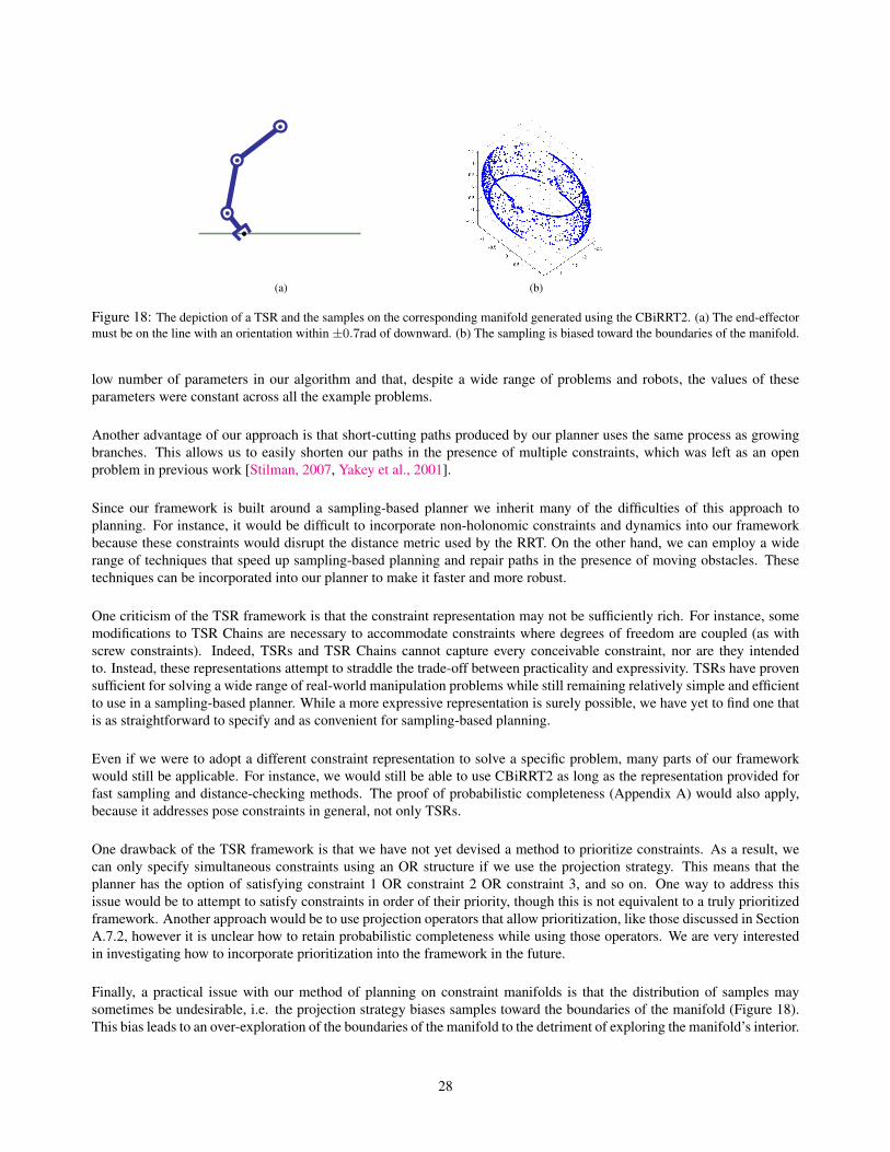
(a) (b)

Figure 18: The depiction of a TSR and the samples on the corresponding manifold generated using the CBiRRT2. (a) The end-effectormust be on the line with an orientation within ±0.7rad of downward. (b) The sampling is biased toward the boundaries of the manifold.

low number of parameters in our algorithm and that, despite a wide range of problems and robots, the values of theseparameters were constant across all the example problems.

Another advantage of our approach is that short-cutting paths produced by our planner uses the same process as growingbranches. This allows us to easily shorten our paths in the presence of multiple constraints, which was left as an openproblem in previous work [Stilman, 2007, Yakey et al., 2001].

Since our framework is built around a sampling-based planner we inherit many of the difficulties of this approach toplanning. For instance, it would be difficult to incorporate non-holonomic constraints and dynamics into our frameworkbecause these constraints would disrupt the distance metric used by the RRT. On the other hand, we can employ a widerange of techniques that speed up sampling-based planning and repair paths in the presence of moving obstacles. Thesetechniques can be incorporated into our planner to make it faster and more robust.

One criticism of the TSR framework is that the constraint representation may not be sufficiently rich. For instance, somemodifications to TSR Chains are necessary to accommodate constraints where degrees of freedom are coupled (as withscrew constraints). Indeed, TSRs and TSR Chains cannot capture every conceivable constraint, nor are they intendedto. Instead, these representations attempt to straddle the trade-off between practicality and expressivity. TSRs have provensufficient for solving a wide range of real-world manipulation problems while still remaining relatively simple and efficientto use in a sampling-based planner. While a more expressive representation is surely possible, we have yet to find one thatis as straightforward to specify and as convenient for sampling-based planning.

Even if we were to adopt a different constraint representation to solve a specific problem, many parts of our frameworkwould still be applicable. For instance, we would still be able to use CBiRRT2 as long as the representation provided forfast sampling and distance-checking methods. The proof of probabilistic completeness (Appendix A) would also apply,because it addresses pose constraints in general, not only TSRs.

One drawback of the TSR framework is that we have not yet devised a method to prioritize constraints. As a result, wecan only specify simultaneous constraints using an OR structure if we use the projection strategy. This means that theplanner has the option of satisfying constraint 1 OR constraint 2 OR constraint 3, and so on. One way to address thisissue would be to attempt to satisfy constraints in order of their priority, though this is not equivalent to a truly prioritizedframework. Another approach would be to use projection operators that allow prioritization, like those discussed in SectionA.7.2, however it is unclear how to retain probabilistic completeness while using those operators. We are very interestedin investigating how to incorporate prioritization into the framework in the future.

Finally, a practical issue with our method of planning on constraint manifolds is that the distribution of samples maysometimes be undesirable, i.e. the projection strategy biases samples toward the boundaries of the manifold (Figure 18).This bias leads to an over-exploration of the boundaries of the manifold to the detriment of exploring the manifold’s interior.

28

It can cause the algorithm to perform slowly if an interior point of the manifold is needed to complete a path. On the otherhand, the algorithm is much faster at finding configurations on the boundary, which can be useful for problems such as theweight-lifting example, where the robot must slide the dumbbell to the edge of the table in order to lift it.

10 Conclusion

We have presented a practical framework for representing and planning with end-effector pose constraints, among others.The underpinnings of our approach are the TSR and TSR Chain representations, which allow us to easily specify constraintsfor a given problem. These representations are designed specifically for sampling-based planners and as a result possessfast sampling and distance-checking methods. The TSR framework uses these representations to characterize and solvemany real-world problems ranging from reaching to grasp to manipulating articulated objects. Most importantly, theframework is designed for real-world robots, such as the mobile manipulator and humanoid shown earlier. We discussthe completeness properties of planning with end-effector pose constraints and present a proof for a class of planningalgorithms in Appendix A. This provides a theoretical foundation for our framework and reinforces its generality. Finally,we have begun to apply our framework to planning with uncertainty, where we developed a method that exploits freedomsin task specification to compensate for uncertainty in object pose.

11 Acknowledgements

This research was partially supported by Intel Labs Pittsburgh and by the National Science Foundation under Grant No.EEC-0540865. Thanks to Ross Knepper, Julius Ziegler, Joel Chestnut, Nico Blodow, and David Handron for helpfuldiscussions.

A Appendix: Probabilistic Completeness

We now discuss a proof of probabilistic completeness for our approach to planning with end-effector pose constraints. Sincethe proof is quite lengthy, we provide only a summary here (for details see [Berenson and Srinivasa, 2010]). We emphasizethat this proof is valid for a class of algorithms that plan with constraints on end-effector pose, not only CBiRRT2. Wealso note that, while we focus on the TSR representation in the rest of this paper, this section makes no assumptions aboutthe representation of pose constraints. Our only restriction is that the dimensionality of the manifold described by theconstraint is fixed for a given problem.

Depending on the definition of an end-effector pose constraint, it can induce a variety of manifolds in the robot’s configu-ration space. If these manifolds have non-zero volume in the C-space (see Figure 19d) it is straightforward to show that anRRT-based algorithm is probabilistically complete because rejection sampling in the C-space will eventually place samplesinside of the manifold. However, if a pose constraint induces a lower-dimensional manifold, i.e. one that has zero volumein the C-space (see Figures 19e and 19f), rejection sampling in the C-space will not generate a sample on the constraintmanifold.

RRT-based algorithms can overcome this problem by using the projection strategy: sampling coupled with a projectionoperator to move configuration space samples onto the constraint manifold. However, it is not clear whether the projec-tion strategy produces adequate coverage of the constraint manifold to guarantee probabilistic completeness. The proofpresented in this section guarantees probabilistic completeness for a class of RRT-based algorithms given an appropriateprojection operator. This proof is valid for constraint manifolds of any fixed dimensionality.

29

(a) (b) (c)

(d) (e) (f)

Figure 19: Three pose constraints and their corresponding C-space constraint manifolds for a 3-link manipulator. (a) The end-effectormust be in the green rectangle with an orientation ±0.7rad of downward. (b) The end-effector must be on the line with an orientation±0.7rad of downward. (c) The end-effector must be on the line pointing downward. (d-f) show graphs created from sampling on themanifolds corresponding to the constraints in (a-c), respectively. Black points are nodes and blue lines are edges. The manifold in (d)has non-zero volume in the C-space, the manifolds in (e) and (f) do not.

Name Symbol Dimension

C-space Q nConfiguration q 0

Constraint Manifold M m = n− (r − d)Reachability R r

Pose x(q) 0Task Constraint T d ≤ r

TABLE A.1: DEFINITIONS USED THROUGHOUT THE PROOF OF PROBABILISTIC COMPLETENESS.

Our proof of probabilistic completeness has two parts: first, we present a set of properties for the projection operator andprove that these properties allow the projection strategy to cover the constraint manifold. Second, we describe a class ofRRT-based algorithms (such as CBiRRT2 and TCRRT [Stilman, 2007]), which use such a projection operator and provethat they are probabilistically complete.

A.1 Definitions

A topological manifold is a second-countable Hausdorff space where every point has a neighborhood homeomorphic toan open Euclidean n-ball, where n is allowed to vary. Manifolds can be disjoint, with each piece of the manifold called aconnected component. Manifolds that have a fixed n (i.e. n-dimensional manifolds) are called pure manifolds.

Let µn be a measure of volume in an n-dimensional space. If the volume of a manifold in an embedding space is zero, thenthe probability of generating a sample on the manifold by rejection sampling in the embedding space is zero. Converselyif the volume of a manifold in an embedding space is not zero, then the probability of generating a sample on the manifoldby rejection sampling in the embedding space will go to 1 as the number of samples goes to infinity.

A sampling method covers a manifold if it generates a set of samples such that any open n-dimensional ball contained inthe manifold contains at least one sample.

30

Our proof of manifold coverage hinges on the concept of self-motion manifolds, which were described in [Burdick, 1989].A self-motion manifold is the set of configurations in C-space which place the end-effector of the robot in a certain pose.

Let the reachable manifold of end-effector poses of the given manipulator be R ⊆ SE(3). R is defined by the ForwardKinematics function of the robot:

x : Q → R (21)

where Q is the C-space. x is always surjective and can be one-to-one or many-to-one, depending on the manipulator. Werestrict our proof to manipulators whose Q andR are both pure manifolds.

Let Q be n-dimensional, where n is the number of DOF of the manipulator. We will parameterize SE(3) locally usingthree variables for translation and three for rotation, i.e. a pose will be a vector in R6. Let R be r-dimensional, wherer ≤ 6.

Let the manifold of end-effector poses allowable by the task be T ⊆ R. Let this manifold have dimensionality d ≤ r. Wewill assume that d is fixed, though we will discuss the implications of allowing d to vary in Section A.7. Let the manifoldof configurations that place the robot’s end-effector in T beM⊆ Q.M is the union of all self-motion manifolds that mapto a pose in T :

M =⋃t∈T{q ∈ Q | x(q) = t} (22)

M has dimensionality m = n− (r − d).

We will be using the (weighted-)Euclidian distance metric on SE(3), which we will denote as dist. This distance metrichas the property that each pose in T has at least an (r − d)-dimensional Voronoi cell in R. A Voronoi cell is the set ofpoints that are closer to a certain point than to any other given a distance metric [LaValle, 2006].

Table A.1 summarizes the definitions and dimensionalities of manifolds used in the proof.

A.2 Proof of manifold coverage by the projection strategy

The projection strategy first produces a sample in the C-space and then projects that sample onto M using a projectionoperator P : Q → M. In order to show that an algorithm using the projection strategy is probabilistically complete, wemust first show that this method coversM.

This section will show that the projection strategy does indeed cover M if the projection operator has the followingproperties:

1. P (q) = q if and only if x(q) ∈ T

2. If x(q1) is closer to x(q2) ∈ T than to any other point in T and dist(x(q1), x(q2)) < ε for an infinitesimal ε > 0,then x(P (q1)) = x(q2).

31

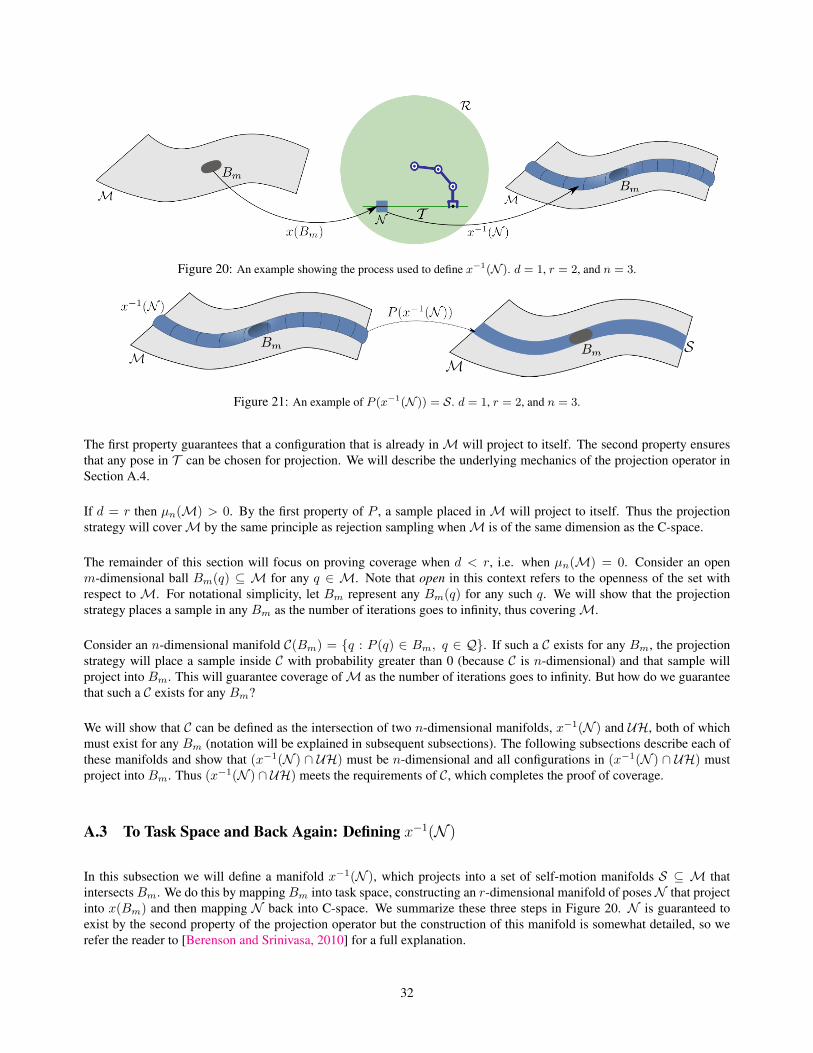
Figure 20: An example showing the process used to define x−1(N ). d = 1, r = 2, and n = 3.

Figure 21: An example of P (x−1(N )) = S. d = 1, r = 2, and n = 3.

The first property guarantees that a configuration that is already inM will project to itself. The second property ensuresthat any pose in T can be chosen for projection. We will describe the underlying mechanics of the projection operator inSection A.4.

If d = r then µn(M) > 0. By the first property of P , a sample placed inM will project to itself. Thus the projectionstrategy will coverM by the same principle as rejection sampling whenM is of the same dimension as the C-space.

The remainder of this section will focus on proving coverage when d < r, i.e. when µn(M) = 0. Consider an openm-dimensional ball Bm(q) ⊆ M for any q ∈ M. Note that open in this context refers to the openness of the set withrespect to M. For notational simplicity, let Bm represent any Bm(q) for any such q. We will show that the projectionstrategy places a sample in any Bm as the number of iterations goes to infinity, thus coveringM.

Consider an n-dimensional manifold C(Bm) = {q : P (q) ∈ Bm, q ∈ Q}. If such a C exists for any Bm, the projectionstrategy will place a sample inside C with probability greater than 0 (because C is n-dimensional) and that sample willproject into Bm. This will guarantee coverage ofM as the number of iterations goes to infinity. But how do we guaranteethat such a C exists for any Bm?

We will show that C can be defined as the intersection of two n-dimensional manifolds, x−1(N ) and UH, both of whichmust exist for any Bm (notation will be explained in subsequent subsections). The following subsections describe each ofthese manifolds and show that (x−1(N ) ∩ UH) must be n-dimensional and all configurations in (x−1(N ) ∩ UH) mustproject into Bm. Thus (x−1(N ) ∩ UH) meets the requirements of C, which completes the proof of coverage.

A.3 To Task Space and Back Again: Defining x−1(N )

In this subsection we will define a manifold x−1(N ), which projects into a set of self-motion manifolds S ⊆ M thatintersectsBm. We do this by mappingBm into task space, constructing an r-dimensional manifold of posesN that projectinto x(Bm) and then mapping N back into C-space. We summarize these three steps in Figure 20. N is guaranteed toexist by the second property of the projection operator but the construction of this manifold is somewhat detailed, so werefer the reader to [Berenson and Srinivasa, 2010] for a full explanation.

32

The manifold produced at the end of the three-step process is x−1(N ), which has the following properties:

1. x−1(N ) is n-dimensional.

2. x−1(N ) contains Bm

3. P (x−1(N )) = S

S is defined as the manifold of configurations which map into x(Bm); i.e. S = {q ∈ M | x(q) ∈ x(Bm)} (see Figure21). We will use S to show coverage ofM in Section A.5.

S has the following properties:

1. If a self-motion manifold intersects Bm, it is a subset of S.

2. If a self-motion manifold does not intersect Bm, it is not a subset of S.

3. S 6= ∅.

A.4 Projection into a ball on a self-motion manifold

We have shown that P (x−1(N )) = S and described some properties of S, however we have not stated where on S aprojected configuration will go. It is possible that a q ∈ x−1(N ) will project to a configuration outside of Bm because Smay contain configurations outside of Bm (see Figure 21).

In order to show that the probability of placing a sample inside Bm using the projection strategy is greater than 0, we needto show that there exists an n-dimensional manifold around a ball on a self-motion manifold that projects into that ball.The purpose of this subsection is to prove this property of self-motion manifolds. The remainder of this subsection willconsider a self-motion manifold in isolation in order to show this property.

Let us now look closer at the mechanism of projection used by P . In this paper, we focus on projection operators basedon Jacobian pseudo-inverse or Jacobian transpose. These kinds of projection operators step towards a pose target and thisprocess can be written as a differential equation:

dq

dt= f(q(t)), t ∈ [0,∞) (23)

An equilibrium point q of Equation 23 satisfies f(q) = 0. q is asymptotically stable if any q(0) inside a neighborhoodcontaining q will converge to q as the number of iterations of Equation 23 goes to infinity.

The set of equilibrium points for the task of placing the end-effector at a given pose is the self-motion manifold Q, which is(n− r)-dimensional. In [Berenson and Srinivasa, 2010], we showed that, for any q ∈ Q, there exists an r-dimensional ballBr(q) within which the conditions for asymptotic stability hold. Thus the evolution of Equation 23 results in the projectionP (q(0)) = q for all q ∈ Q, for all q(0) ∈ Br(q). Note that this fact is only valid for a self-motion manifold in isolation.

Let us now consider an open (n − r)-dimensional ball BQ(q) ⊆ Q. Define H(BQ(q)) as the manifold Br(q) × BQ(q)embedded in Q (see Figure 22).

H has the following properties:

33

Figure 22: A self-motion manifold in C-space. r = 2 and n = 3.

Figure 23: An example of C = (x−1(N ) ∩ UH). d = 1, r = 2, and n = 3.

1. H is n-dimensional.

2. H contains BQ(q).

3. P (q) ∈ BQ(q) for all q ∈ H (conditional).

It is important to note that we have only described H for a self-motion manifold in isolation. The third property of H isonly valid when x(q) is closer to x(Q) than to any x(k), for a self-motion manifold k ⊆ (M− Q). I.e. the third propertyholds only when Q is “chosen” by the projection operator.

A.5 Putting it all together

We will now bring the concepts developed thus far together to show coverage ofM by the projection strategy. Recall that,to show coverage ofM, we must show that the projection strategy places a sample inside any Bm ⊆M.

Section A.3 showed that a configuration inside x−1(N ) will project into S, which consists of all self-motion manifolds thatintersectBm. Let us construct an n-dimensional manifold UH(Bm) by taking the union of the n-dimensionalHmanifoldsaround every Q ∩Bm for all Q ⊆ S:

UH(Bm) =⋃Q⊆S

H(Q ∩Bm) (24)

UH inherits the properties of H, as well as the condition on the third property: A configuration q ∈ UH will project toa configuration inside Bm by the third property of H if, for some Q ⊆ S , x(q) is closer to x(Q) than to any x(k), for aself-motion manifold k ⊆ (M−S).

Let C = (x−1(N ) ∩ UH) (see Figure 23). C has the following properties:

1. C is n-dimensional.

2. P (q) ∈ Bm for all q ∈ C.

34

Theorem 1 The projection strategy places a sample inside any Bm as the number of samples goes to infinity.

Proof: By the first property of C, µn(C) > 0. Thus the probability of sampling a q ∈ C is greater than 0 and, as the numberof samples goes to infinity, the probability of sampling a q ∈ C goes to 1. P (q) ∈ Bm by the second property of C. Thuswe have shown that the projection strategy places a sample inside any Bm as the number of samples goes to infinity, whichentails that the projection strategy coversM.

A.6 Probabilistic completeness of RRT-Based algorithms using the projection strategy

We can use the fact that the projection strategy covers M to prove that RRT-based methods that plan paths on M areprobabilistically complete. We focus on a class of RRT-based algorithms that plan with end-effector pose constraints, forexample CBiRRT2 and TCRRT [Stilman, 2007]. These algorithms grow trees onM by sampling near an existing nodeonM and then projecting that sample toM. An RRT-based algorithm with the following properties is probabilisticallycomplete:

1. Given a node of the existing tree, the probability of sampling in an n-dimensional ball centered at that node is greaterthan 0 and the sampling covers this ball.

2. The algorithm uses a projection operator with the properties of P to project samples toM.

We know that the algorithm will cover any ball in M centered at an existing configuration in the tree by Theorem 1.We can then use the series-of-balls argument to show that we place a node in any Bm which is connected to the startingconfiguration. The basis of this argument is that we can construct a series of overlapping balls on the manifold whichcontains some node in the tree and overlaps with Bm. We can use Theorem 1 to show that an RRT node will be placedin each region of overlap between subsequent balls until the tree reaches Bm. For a more detailed explanation of theseries-of-balls argument see [Svestka, 1996] and [Kuffner and LaValle, 2000].

Thus we have shown that the RRT can reach any Bm connected to the starting configuration, which entails that the algo-rithm is probabilistically complete.

A.7 Implications of the Proof

We now discuss the implications of our proof for sampling goals, choosing projection operators, and planning with mixed-dimensional constraint manifolds.

A.7.1 Probabilistically Complete Goal Sampling

The above proof also applies to pose goal constraints, where we would like to ensure that projection sampling covers themanifold of configurations corresponding to some set of pose goals in task space. The same principles apply as in the aboveproof, except that we do not rely on a planner to explore the manifold, we simply sample it using the projection strategy. Itfollows clearly from Theorem 1 that this goal manifold will be covered if we sample it using the projection strategy.

35

A.7.2 Projection Operators

Section A.2 describes a projection operator that guarantees probabilistic completeness for RRT-based algorithms. Theregularized Jacobian pseudo-inverse or Jacobian transpose IK methods can be used to perform the projection because theypossess the requisite properties. Unfortunately, there are some common iterative methods which will not yield probabilisticcompleteness.

The null-space projection method [Sentis and Khatib, 2005] operates by using the null-space of the primary task (placingthe end-effector in some pose) to satisfy secondary tasks such as collision-avoidance or balancing. For this method, the dq

dtof Equation 23 is:

dq

dt= J+x+ (I− J+J)qnull (25)

where J+ is the generalized pseudo-inverse of the Jacobian, x is the error in pose, and qnull is the error in meeting asecondary objective. This type of projection attains optimal configurations by sliding along a self-motion manifold whenx = 0. The secondary task induces local minima on the self-motion manifold which attract configurations from the rest ofthe self-motion manifold. Thus, if a ball on the self-motion manifold does not contain a local minimum of the secondarytask, configurations projecting to that ball may escape by sliding along the manifold. It follows that this projection operatorwill not coverM. Though using this projection operator in an RRT-based algorithm may yield an effective planner, it willnot be probabilistically complete.

A.7.3 Mixed-dimensional Constraint Manifolds

The proof of coverage and probabilistic completeness assumed that the pose constraint T had a fixed dimensionality d.If we allow d to vary, then m (the dimensionality ofM) will vary as well. Since our proof of coverage used only localproperties ofM, we can extend this proof to the case of varying m simply by applying the proof to each m-dimensionalcomponent ofM for everym. However, there is the case when a ball around a point onM contains components of varyingdimension. In this case, the ball can be split according to the dimensionality of its components and C can be shown to existfor one of these components, thus guaranteeing a sample will be placed in this ball.

Though we can show that the projection strategy coversM, the proof of probabilistic completeness for RRT-based algo-rithms only holds whenM is pure. The reason is that mixed-dimensional manifolds can be constructed such that all pathsbetween two configurations must go through a narrow passage, which is of lower dimension than any component of themanifold. For instance, supposeM were composed of two lines that intersect at some configuration qp. To get from oneline to the other, the algorithm would need to find a path which contained qp. Yet there is 0 probability of generating qpexactly, thus a path may never be found, though one exists. This difficulty is not caused by the projection strategy and isnot limited only to pose constraints. Rather this difficulty arises for all RRT-based planners when they must find a paththrough a lower-dimensional narrow passage. Coverage ofM does not entail probabilistic completeness in this case. Inorder to guarantee probabilistic completeness, the algorithm must be able to generate samples in these lower-dimensionalnarrow passages, which can be done in a problem-specific way (as in [Hauser and Latombe, 2008]).

References

[Atkeson and Schaal, 1997] Atkeson, C. G. and Schaal, S. (1997). Learning tasks from a single demonstration. In Proc.IEEE International Conference on Robotics and Automation (ICRA), pages 1706–1712.

[Bellman, 1957] Bellman, R. (1957). Dynamic Programming. Princeton University Press, Princeton, NJ.

36

[Bentivegna et al., 2004] Bentivegna, D., Atkeson, C. G., and Cheng, G. (2004). Learning tasks from observation andpractice. Robotics and Autonomous Systems, 47:163–169.

[Berenson et al., 2009a] Berenson, D., Chestnutt, J., Srinivasa, S. S., Kuffner, J. J., and Kagami, S. (2009a). Pose-Constrained Whole-Body Planning using Task Space Region Chains. In Proc. IEEE-RAS International Conferenceon Humanoid Robots (Humanoids09).

[Berenson and Srinivasa, 2010] Berenson, D. and Srinivasa, S. (2010). Probabilistically complete planning with end-effector pose constraints. In IEEE International Conference on Robotics and Automation (ICRA).

[Berenson et al., 2009b] Berenson, D., Srinivasa, S., and Kuffner, J. (2009b). Addressing Pose Uncertainty in Manip-ulation Planning Using Task Space Regions. In Proc. IEEE/RSJ International Conference on Intelligent Robots andSystems (IROS).

[Berenson et al., 2009c] Berenson, D., Srinivasa, S. S., Ferguson, D., Collet, A., and Kuffner, J. (2009c). Manipulationplanning with workspace goal regions. In Proc. IEEE International Conference on Robotics and Automation (ICRA).

[Berenson et al., 2009d] Berenson, D., Srinivasa, S. S., Ferguson, D., and Kuffner, J. (2009d). Manipulation planning onconstraint manifolds. In Proc. IEEE International Conference on Robotics and Automation (ICRA).

[Bertram et al., 2006] Bertram, D., Kuffner, J., Dillmann, R., and Asfour, T. (2006). An integrated approach to inversekinematics and path planning for redundant manipulators. In Proc. IEEE International Conference on Robotics andAutomation (ICRA), pages 1874–1879.

[Burdick, 1989] Burdick, J. (1989). On the inverse kinematics of redundant manipulators: characterization of the self-motion manifolds. In Proc. IEEE International Conference on Robotics and Automation (ICRA), pages 264–270.

[Collet et al., 2009] Collet, A., Berenson, D., Srinivasa, S. S., and Ferguson, D. (2009). Object recognition and full poseregistration from a single image for robotic manipulation. In Proc. IEEE International Conference on Robotics andAutomation (ICRA).

[Cortes and Simeon, 2004] Cortes, J. and Simeon, T. (2004). Sampling-based motion planning under kinematic loop-closure constraints. In Workshop on the Algorithmic Foundations of Robotics (WAFR).

[Devroye, 1986] Devroye, L. (1986). Non-Uniform Random Variate Generation, pages 567–571. Springer-Verlag, NewYork.

[Diankov et al., 2008] Diankov, R., Srinivasa, S. S., Ferguson, D., and Kuffner, J. (2008). Manipulation planning withcaging grasps. In Proc. IEEE-RAS International Conference on Humanoid Robots (Humanoids 08).

[Drumwright and Ng-Thow-Hing, 2006] Drumwright, E. and Ng-Thow-Hing, V. (2006). Toward interactive reaching instatic environments for humanoid robots. In Proc. IEEE/RSJ International Conference on Intelligent Robots and Systems(IROS).

[Hauser and Latombe, 2008] Hauser, K. and Latombe, J. (2008). Multi-Modal Motion Planning in Non-Expansive Spaces.In Workshop on the Algorithmic Foundations of Robotics (WAFR).

[Hirano et al., 2005] Hirano, Y., Kitahama, K., and Yoshizawa, S. (2005). Image-based object recognition and dexteroushand/arm motion planning using rrts for grasping in cluttered scene. In Proc. IEEE/RSJ International Conference onIntelligent Robots and Systems (IROS).

[Howard et al., 2008] Howard, M., Klanke, S., Gienger, M., Goerick, C., and Vijayakumar, S. (2008). Learning potential-based policies from constrained motion. In Proc. 8th IEEE-RAS International Conference on Humanoid Robots (Hu-manoids 08).

[Kavraki et al., 1996] Kavraki, L. E., Svestka, P., Latombe, J. C., and Overmars, M. H. (1996). Probabilistic roadmaps forpath planning in high-dimensional configuration spaces. IEEE Transactions on Robotics and Automation, 12(4):566–580.

37

[Khatib, 1987] Khatib, O. (1987). A unified approach for motion and force control of robot manipulators: The operationalspace formulation. IEEE Transactions on Robotics and Automation, 3(1):43–53.

[Koga et al., 1994] Koga, Y., Kondo, K., Kuffner, J., and claude Latombe, J. (1994). Planning motions with intentions. InSIGGRAPH.

[Kuffner and LaValle, 2000] Kuffner, J. J., J. and LaValle, S. M. (2000). RRT-connect: An efficient approach to single-query path planning. In Proc. IEEE International Conference on Robotics and Automation (ICRA).

[LaValle and Kuffner, 2000] LaValle, S. and Kuffner, J. (2000). Rapidly-exploring random trees: Progress and prospects.In Workshop on the Algorithmic Foundations of Robotics (WAFR).

[LaValle, 2006] LaValle, S. M. (2006). Planning Algorithms. Cambridge University Press, Cambridge, U.K.

[Oriolo and Mongillo, 2005] Oriolo, G. and Mongillo, C. (2005). Motion planning for mobile manipulators along givenend-effector paths. In Proc. IEEE International Conference on Robotics and Automation (ICRA).

[Oriolo et al., 2002] Oriolo, G., Ottavi, M., and Vendittelli, M. (2002). Probabilistic motion planning for redundant robotsalong given end-effector paths. In Proc. IEEE/RSJ International Conference on Intelligent Robots and System (IROS).

[Sciavicco and Siciliano, 2000] Sciavicco, L. and Siciliano, B. (2000). Modeling and Control of Robot Manipulators,pages 96–100. Springer, 2nd edition.

[Seereeram and Wen, 1995] Seereeram, S. and Wen, J. (1995). A global approach to path planning for redundant manip-ulators. IEEE Transactions on Robotics and Automation, 11(1):152–160.

[Sentis and Khatib, 2005] Sentis, S. and Khatib, O. (2005). Synthesis of whole-body behaviors through hierarchical con-trol of behavioral primitives. International Journal of Humanoid Robotics, 2:505–518.

[Stilman, 2007] Stilman, M. (2007). Task constrained motion planning in robot joint space. In Proc. IEEE/RSJ Interna-tional Conference on Intelligent Robots and Systems (IROS).

[Stilman et al., 2007] Stilman, M., Schamburek, J. U., Kuffner, J., and Asfour, T. (2007). Manipulation planning amongmovable obstacles. In Proc. IEEE International Conference on Robotics and Automation (ICRA).

[Sugihara and Nakamura, 2002] Sugihara, T. and Nakamura, Y. (2002). Whole-body cooperative balancing of humanoidrobot using cog jacobian. In Proc. IEEE/RSJ International Conference on Intelligent Robots and Systems (IROS).

[Svestka, 1996] Svestka, P. (1996). On probabilistic completeness and expected complexity of probabilistic path planning.Technical report, UU-CS-96-20. Department of Computer Science, Utrecht University, Utrecht, Netherlands.

[Vande Weghe et al., 2007] Vande Weghe, M., Ferguson, D., and Srinivasa, S. S. (2007). Randomized path planning forredundant manipulators without inverse kinematics. In Proc. IEEE-RAS International Conference on Humanoid Robots(Humanoids 07).

[Walker and Orin, 1982] Walker, M. and Orin, D. (1982). Efficient dynamic computer simulation of robotic mechanisms.ASME Journal of Dynamic Systems Measurement and Control, 104:205–211.

[Yakey et al., 2001] Yakey, J. H., LaValle, S. M., and Kavraki, L. E. (2001). Randomized path planning for linkages withclosed kinematic chains. IEEE Transactions on Robotics and Automation, 17(6):951–958.

[Yamane et al., 2004] Yamane, K., Kuffner, J., and Hodgins, J. (2004). Synthesizing animations of human manipulationtasks. In SIGGRAPH.

[Yao and Gupta, 2005] Yao, Z. and Gupta, K. (2005). Path planning with general end-effector constraints: using taskspace to guide configuration space search. In Proc. IEEE/RSJ International Conference on Intelligent Robots andSystems (IROS).

38