Task-level approaches for the control of constrained ...nmbl.stanford.edu/publications/pdf/Desapio2006.pdf · Springer ScienceC +Business Media B.V. 2006 Abstract This paper presents

Multibody Syst Dyn (2006) 16:73–102DOI 10.1007/s11044-006-9017-3

Task-level approaches for the control of constrainedmultibody systems

Vincent De Sapio · Oussama Khatib · Scott Delp

Received: 29 September 2005 / Accepted: 6 April 2006C© Springer Science + Business Media B.V. 2006

Abstract This paper presents a task-level control methodology for the general class of holo-nomically constrained multibody systems. As a point of departure, the general formulationof constrained dynamical systems is reviewed with respect to multiplier and minimizationapproaches. Subsequently, the operational space framework is considered and the underlyingsymmetry between constrained dynamics and operational space control is discussed. Moti-vated by this symmetry, approaches for constrained task-level control are presented whichcast the general formulation of constrained multibody systems into a task space setting us-ing the operational space framework. This provides a means of exploiting task-level controlstructures, native to operational space control, within the context of constrained systems.This allows us to naturally synthesize dynamic compensation for a multibody system, thatproperly accounts for the system constraints while performing a control task. A set of exam-ples illustrate this control implementation. Additionally, the inclusion of flexible bodies inthis approach is addressed.

Keywords Task-level control . Constrained multibody dynamics . Operational space . Nullspace . Flexible/rigid multibody system

1. Introduction

The control of multibody systems is of interest to a number of research communities in avariety of application areas. In particular, the robotics community has focussed on the controlof high degree-of-freedom robotic systems. Typically, this has involved the control of serial

V. De Sapio (�) · O. KhatibArtificial Intelligence Laboratory, Computer Science Department, Stanford University, Stanford,CA 94305, USAe-mail: [email protected]

S. DelpNeuromuscular Biomechanics Laboratory, Mechanical Engineering & Bioengineering Departments,Stanford University, Stanford, CA 94305, USA

Springer

74 Multibody Syst Dyn (2006) 16:73–102

Fig. 1 Parallel mechanisms consisting of serial chains with loop closures described by a set of holonomicconstraints. (Left) A spatial positioning platform [7]. (Right) Bilateral representation of a parallel-serial roboticshoulder mechanism [24]

and branching chain systems. The traditional approach for controlling these systems has beenjoint space (ie., configuration space) control. The operational space approach was introducedby Khatib [19, 20] to simplify the control problem by specifying a task space rather than ajoint space control objective. Task space is used interchangeably with operational space torefer to the space of motion control coordinates. As one simple example, the task space forcontrolling a robot arm can be defined as the Cartesian space used to describe the positionof the end effector. Using the operational space approach the configuration space dynamicsof a multibody system are mapped into an appropriate task space. This is advantageous forcontrol purposes since the operational space method provides task-level dynamic models andstructures for decoupled task and posture control. This allows for posture objectives to becontrolled without dynamically interfering with the primary task(s).

The benefits of operational space control have been primarily exploited for serial andbranching chain systems. However, there has been substantially less emphasis on the use ofoperational space control for closed chain or parallel systems, like the structures of Figure 1[7]. Closed chains are a subset of the larger class of holonomically constrained systems whichinclude biomechanical structures such as the knee and shoulder complex of Figure 2. Rather

Fig. 2 Holonomic constraints provide more physiologically representative models. (Left) The tibia translatesas a function of knee flexion [9]. (Right) The shoulder girdle (scapula and clavicle) is kinematically coupledto the glenohumeral joint [14]

Springer

Multibody Syst Dyn (2006) 16:73–102 75

than loop closures these examples involve constraints internal to the branching chains [9, 14],expressed as algebraic dependencies between the generalized coordinates.

This paper addresses the use of task-level approaches for the control of holonomically con-strained multibody systems. As a point of departure, the general formulation of constraineddynamical systems is reviewed. This entails an elaboration of multiplier and minimizationforms of the constrained multibody equations of motion. The basis for task-level control isthen presented with a review of the operational space method. Operational space dynamicconsistency provides a mechanism for exploring the underlying symmetry between taskand constraint dynamics. Formulations for constrained task-level control are then presented,punctuated with a set of examples. Finally, the inclusion of flexible bodies in this approachis discussed.

2. Constrained dynamics

The subsequent sections review the dynamical formulation of constrained multibody systems.This review covers the well known method of Lagrange multipliers, a multiplier eliminationmethod, and the less well known minimization formalism of Gauss’ Principle. This latterformalism naturally leads to an explicit solution of the constrained dynamical system andthe subsequent formulation of a generalized constrained equation of motion. The multiplierform, the eliminated multiplier form, and the generalized constrained form will each be usedin Section 5 to formulate novel methods for constrained operational space control.

2.1. Unconstrained systems

The equations of motion for a multibody system that is unconstrained with respect to con-figuration space are expressed in standard form as [3],

M(q) q + b(q, q) = f (q, q) + B(q, q)T u (1)

where q is the n × 1 vector of generalized coordinates, u is the k × 1 vector of controlinputs, B(q, q)T is the n × k matrix mapping control inputs to generalized actuator forces,M(q) is the n × n mass matrix, b(q, q) is the n × 1 vector of centrifugal and Coriolis terms,and f (q, q) is the n × 1 vector of generalized applied forces. For conciseness we will oftenrefrain from explicitly denoting the functional dependence of these quantities on q and q .This practice will also be employed with other quantities as well.

Throughout this paper we will use a modified and more specialized form of (1) commonin robotics [6],

τ = M(q) q + b(q, q) + g(q) (2)

where τ is the n × 1 vector of generalized actuator forces (torques) and g(q) is the n × 1vector of gravity terms. The form of (2) assumes that the generalized actuator forces can bedirectly interpreted as control inputs; that is,τ = BT u = u, ie. BT = 1. Additionally, the gen-eralized applied forces are assumed to be restricted to gravity terms; that is, f (q, q) = −g(q).This second assumption is relatively minor and will not limit the generality of the approachespresented in this paper. The first assumption regarding the control inputs restricts our exam-ination to fully actuated systems. However, this limitation can be overcome by introducing

Springer


a selection matrix (similar to BT in mapping actuator control inputs to generalized actuatorforces). We utilize this for a partial examination of under-actuated systems in Section 5.

2.2. Multiplier form of the system dynamics

We introduce a set of mC holonomic and scleronomic constraint equations, φ(q) = 0, thatare satisfied on a p = n − mC dimensional manifold, Q p, in configuration space, Q = Rn .The gradient ofφ yields the mC × n constraint Jacobian matrix, Φ. Adjoining the constraintsto (2) by introducing a set of constraint forces yields the dynamic equation,

τ = Mq + b + g − τC (3)

subject to,

Φq + Φq = 0 (φ = 0, Φq = 0) (4)

where τC is the vector of generalized constraint forces. The variation of the constraint equa-tions yields δφ(q) = Φ δq = 0, which implies δq ∈ ker(Φ). The operator ker() representsthe kernel of a matrix and in this context will be synonymous with the null space of a ma-trix throughout this paper. Since the constraints do no virtual work under these constraintconsistent virtual displacements we have,

τC⊥ δq ∀ δq ∈ ker(Φ) (5)

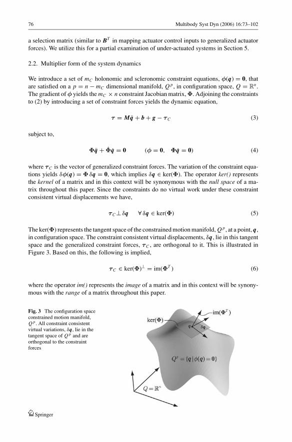
The ker(Φ) represents the tangent space of the constrained motion manifold, Q p, at a point, q ,in configuration space. The constraint consistent virtual displacements, δq , lie in this tangentspace and the generalized constraint forces, τC , are orthogonal to it. This is illustrated inFigure 3. Based on this, the following is implied,

τC ∈ ker(Φ)⊥ = im(ΦT ) (6)

where the operator im() represents the image of a matrix and in this context will be synony-mous with the range of a matrix throughout this paper.

Fig. 3 The configuration spaceconstrained motion manifold,Q p . All constraint consistentvirtual variations, δq, lie in thetangent space of Q p and areorthogonal to the constraintforces

Springer


Thus, the generalized constraint force can be represented as a linear combination of thecolumns of ΦT . That is, τC = ΦTλ, where λ is a vector of unknown Lagrange multipliers.The constrained multibody equations of motion, expressed in the familiar multiplier form,are thus,

τ = Mq + b + g − ΦTλ (7)

subject to (4).

2.3. Elimination of multipliers

The Lagrange multipliers can be eliminated from (7) by first expressing the zeroth ordervariational equation,

τC · δq + (τ − Mq − b − g) · δq = 0 (8)

By restricting the variations to constraint consistent virtual displacements we have,

τC · δq + (τ − Mq − b − g) · δq = 0

∀ δq ∈ ker(Φ)(9)

Recalling (5) we note that the generalized constraint forces produce no virtual work undervirtual displacements that are consistent with the constraints. Thus, the term τC · δq vanishesfrom (9) and we have the following orthogonality relation,

(Mq + b + g − τ ) · δq = 0

∀ δq ∈ ker(Φ)(10)

We now define a matrix, C ∈ Rn×p, whose columns span the null space of Φ. This im-plies that im(C) = ker(Φ). Thus, ΦC = 0 and CT ΦT = 0. In this manner C orthogonallycomplements Φ. That is,

im(C) = ker(Φ) = im(ΦT )⊥ (11)

Geometrically, im(C) represents the tangent space of the constrained motion manifold, Q p

(see Figure 3). These geometric properties are discussed in further detail in [2, 17]. While notrequired for the subsequent analysis we specify that the columns of C be mutually orthogonaland thus form an orthogonal basis, C, for the null space of Φ. The constraint consistent virtualdisplacements, δq ∈ ker(Φ), can then be expressed in terms of the virtual displacements ofa minimal set of p independent coordinates, q p,

δq = C δq p (12)

Springer


Using this relationship we can express (10) over all possible variations of a minimal set ofcoordinates,

(CT Mq + CT b + CT g − CT τ ) · δq p = 0

∀ δq p ∈ Rp

⇓CT τ = CT Mq + CT b + CT g

(13)

Noting that q = Cq p and q = Cq p + Cq p we can express (13) as,

τp = Mp(q) q p + bp(q, q p) + g p(q) (14)

where,

Mp(q) = CT MC

bp(q, q p) = CT b + CT MCq p(15)

g p(q) = CT g

τp = CT τ

The approach outlined here is well known in multibody dynamics and is consistent with theprojection method of [2]. This approach was also used by Russakow et al. for applicationto serial-to-parallel chain manipulators [31]. We note that (14) includes a mix of our initialset of n generalized coordinates, q, as well as the minimal set of p independent coordinates,q p. Since the constraints are holonomic we would expect there to be a mapping, in principle,which could be derived from the constraints that would yield q = q(q p). In this case C couldbe computed explicitly from the mapping rather than computing the null space of Φ; that is,C = ∂q/∂q p. Additionally, the terms in (14) could be expressed as functions of q p rather thanq. Since q p are independent coordinates the constraints would be implicitly addressed andthe resulting system would be unconstrained with respect to configuration space. However,finding the mapping q = q(q p) would be difficult in general. In such cases a null spacemethod or a coordinate partitioning method [36] would need to be used to compute C .

Additionally, the generalized coordinates, q p, and the generalized forces, τ p, do notnecessarily have a natural and physically intuitive meaning, making it difficult to standardizetheir use in a numerical algorithm. This is in contrast to the coordinates, q, which are chosenspecifically to describe the system in the most natural and physically intuitive manner. Itis usually desirable to select q in a manner that preserves the physical meaning of thegeneralized forces as torques about individual joints. Often when using a minimal set ofcoordinates this is not the case, since a single generalized coordinate may influence multiplejoint displacements. Therefore, from an algorithmic perspective it is often preferable to dealwith a non-minimal but standardized set of generalized coordinates (like joint angles) thatare amenable to numerical formulation, and compute the dynamic terms corresponding tothat kinematic parametrization. Equation (14) can then be used, as is, parameterized in termsof q .

Springer


2.4. Minimization form of the system dynamics

By expressing the zeroth order variational Equation (9) we arrive at an orthogonality relation(10). Higher order variations yield similar orthogonality relations. In the particular case ofsecond order variations, known as virtual accelerations, we can arrive at a minimizationprinciple. This was first demonstrated by Gauss [11] and later investigated by Gibbs [12] inmodified form. We begin by first expressing the second order variational form of (3),

τC · δq + (τ − Mq − b − g) · δq = 0 (16)

The virtual accelerations, δq, refer to all acceleration variations which satisfy the constraintswhile time, position, and velocity are fixed. Since we are assuming scleronomic constraintswe only need to be concerned with position and velocity remaining fixed. Given δq = 0 andδq = 0 the variation of (4) yields,

δ(Φq + Φq) = Φ δq = 0 (17)

which implies that δq ∈ ker(Φ). Under this condition (16) can be restricted to constraintconsistent virtual accelerations,

τC · δq + (τ − Mq − b − g) · δq = 0

∀ δq ∈ ker(Φ)(18)

Recalling (5) we have,

τC⊥ δq ∀ δq ∈ ker(Φ) (19)

Thus the term τC · δq vanishes from (18) and we have the following orthogonality relation,

(Mq + b + g − τ ) · δq = 0

∀ δq ∈ ker(Φ)(20)

subject to (4). At this point we introduce the Gauss function, G, defined as a mass-weighteddistance measure between the constrained and unconstrained accelerations,

G �1

2(q − q�)T M(q − q�) (21)

where q� is the unconstrained acceleration of the system. That is, q� is the generalizedacceleration that the system would exhibit in the absence of constraints,

q� = M−1(τ − b − g) (22)

Taking the gradient of G with respect to q yields,

∂G∂q

= M(q − q�) = Mq + b + g − τ (23)

Springer


Fig. 4 The Gauss function, G, isminimized subject to theconstraints. At the solution point,q , the gradient of G is orthogonalto the space of virtualaccelerations. Geometrically, thesolution minimizes the distance(mass-weighted) to theunconstrained acceleration, q�

Substituting (23) into (20) yields,

∂G∂q

· δq = 0 ∀ δq ∈ ker(Φ) (24)

This implies that the solution of the constrained multibody dynamics problem yields a sta-tionary value of G over the set of constraint consistent accelerations, or,

δG = 0 ∀ δ | δq ∈ ker(Φ) (25)

Subject to (4). This is illustrated geometrically in Figure 4 and expresses Gauss’ Principle ofLeast Constraint [4, 30, 34]. These conditions require that the actual generalized acceleration,q, result in a stationary value of the Gauss function, G, and be consistent with the constraints.Moreover, since G is a quadratic form and M is symmetric positive definite, q must minimizeG subject to the constraints.

2.5. Solution of the constrained dynamics problem

As we have seen, the problem of constrained multibody dynamics can be stated as a multiplierproblem or a minimization problem. Both of these statements are equivalent. That is, thesolution of the multiplier problem minimizes the Gauss function, G, over the set of constraintconsistent accelerations and the solution of the minimization problem satisfies the multiplierequations.

We can arrive at an explicit solution of the constrained dynamics problem. Using (22) wecan express (7) and (4) as,

M(q − q�) = ΦTλ(26)

Φq + Φq = 0

It is straightforward to solve this system. The solution yields,

q = −M−1ΦT (ΦM−1ΦT )−1(Φq� + Φq) + q�(27)

λ = −(ΦM−1ΦT )−1(Φq� + Φq)

Springer


We now express the mass-weighted (right) inverse of Φ,

Φ = M−1ΦT (ΦM−1ΦT )−1 (28)

where ΦΦ = 1 and, equivalently, ΦT ΦT = 1. We then have,

q = −ΦΦq + (1 − ΦΦ)q� (29)

Defining the n × n constraint null space matrix, Θ � 1 − ΦΦ, we can write,

q = −ΦΦq + Θq� (30)

Since this solution satisfies Gauss’ Principle we know that it minimizes G while satisfyingthe constraints. The mass weighted inverse, Φ, of the constraint matrix therefore yields thesolution of (4) which minimizes G.

It is noted that Φ and Θ satisfy the condition ΦΘ = 0 and, equivalently, ΘT ΦT = 0.Further, if we form the projection matrix PT = P which projects any vector in Rn onto thenull space of Φ we have,

PT = CCT = 1 − ΦT (ΦΦT )−1Φ (31)

where C is the matrix, defined in Section 2.3, which spans the null space of Φ. The expressionfor PT in (31) has a similar form as the expression,

ΘT = 1 − ΦΦ = 1 − ΦT (ΦM−1ΦT )−1ΦM−1 (32)

Consequently PT = CCT can be regarded as a kinematic constraint null space projectionmatrix and ΘT can be regarded as a mass-weighted constraint null space projection matrix.The physical and geometric meaning of Φ and Θ will be discussed further in Section 4.

2.6. Generalized constrained equation of motion

Given the explicit solution of the constrained dynamics problem (27) we now wish to expressan alternate form of the constrained dynamical equations of motion. We begin by expressingλ in (27) as,

λ = −H[ΦM−1(τ − b − g) + Φq] (33)

where H is the mC × mC constraint space mass matrix which reflects the system inertiaprojected at the constraint,

H � (ΦM−1ΦT )−1 (34)

Substituting (33) into (7) yields,

Mq + b + g = −ΦT HΦq + (1 − ΦT HΦM−1)τ + ΦT HΦM−1(b + g) (35)

Springer


We now define the mC × 1 vector of centrifugal and Coriolis forces projected at the constraint,

α � HΦM−1b − HΦq (36)

and the mC × 1 vector of gravity forces projected at the constraint,

ρ � HΦM−1g (37)

We also note that,

ΘT = 1 − ΦT ΦT = 1 − ΦT HΦM−1 (38)

Substituting these expressions into (35) we have the concise expression which we will referto as the generalized constrained equation of motion,

ΘT τ = Mq + b + g − ΦT (α + ρ) (39)

An alternative means of deriving this equation involves directly mapping the configurationspace Equation (7) into the constraint null space using ΘT ,

ΘT τ = ΘT Mq + ΘT b + ΘT g − ΘT ΦTλ (40)

Noting that ΘT ΦT = 0 and manipulating we have,

ΘT τ = Mq + b + g − ΦT ΦTMq − ΦT ΦT

b − ΦT ΦTg

= Mq + b + g − ΦT HΦq − ΦT (α + ρ) − ΦT HΦq (41)

Substituting in our constraint condition, Φq = −Φq, yields,

ΘT τ = Mq + b + g − ΦT (α + ρ) (42)

3. Task space dynamics

In the previous section we considered configuration space descriptions of the dynamics ofconstrained multibody systems. Our objective is to reformulate these descriptions in thecontext of task space. This will provide the foundation for constrained task-level control tobe discussed in the next section. As a starting point we begin with a review of the basicoperational space framework [19, 20].

The operational space framework addresses the dynamics and control of branching chainrobots. Given a branching chain system the initial step involves defining a set of mT task, oroperational space, coordinates, x. The function x(q) represents a kinematic mapping fromthe set of generalized coordinates to the set of operational space coordinates. The operationalspace coordinates can represent any function of the generalized coordinates but typicallyare chosen to describe the set of control coordinates associated with a motion control task.Figure 5 illustrates simple branching chain systems where the operational space coordinates

Springer


Fig. 5 (Left) A simple task description for a serial chain where the operational space coordinates describe theCartesian position of the terminal point of the chain. (Right) A branching chain where the operational spacecoordinates describe the positions of both terminal points

are chosen to be the Cartesian coordinates associated with positioning the terminal point(s)of the chain. Further, by taking the gradient of x we have the relationship,

x = J(q) q (43)

where J(q) is the mT × n task Jacobian matrix. This relationship applies to both kinematicallynon-redundant and redundant systems. In the case of non-redundant systems the inverse ofthis relationship is well defined outside of singularities. For such cases we have,

q = J−1x (44)

In the redundant case we can define the right inverse of J as,

{J# | J J# = 1} (45)

The solutions to Jq = x are thus given by,

q = J#x + Nqo (46)

where N � 1 − J# J and qo is an arbitrary vector in Rn .At this point we can address operational space kinetics. In the non-redundant case any

generalized force can be produced by an operational space force, f , acting at the task pointalong the task coordinates. Figure 5 illustrates the action of the operational space force forthe intuitive case of Cartesian positioning tasks. The generalized force is then composed asJT f . In the redundant case an additional term needs to complement the task term in orderto realize any arbitrary generalized force. We will refer to this term as the null space termand it can be composed as NT τ o, where NT is the null space projection matrix. An arbitrarygeneralized force, τ , can then be expressed as,

τ = JT f + NT τ o = Mq + b + g (47)

Springer


We can pre-multiply (47) by J M−1 and rearrange to get,

x = J M−1 JT f + J M−1 NT τ o − J M−1b − J M−1g + Jq (48)

where we note that x = Jq + Jq . We can now impose the condition that the term associatedwith the null space, NT τ o, does not contribute to the operational space acceleration. This isreferred to as dynamic consistency [20] and is expressed as,

J M−1 NT τ o = J M−1(1 − JT JT #)τ o = 0, ∀ τ o ∈ Rn (49)

We can solve for J# under this condition and denote this solution as J, the dynamicallyconsistent (right) inverse of J [20],

J = M−1 JT (J M−1 JT )−1 (50)

This represents a unique right inverse of J where, by construction, the null space projectionmatrix, NT = 1 − JT J

T, is guaranteed not to influence the task acceleration. Under this

condition we can manipulate (48) to arrive at,

f = (J M−1 JT )−1x + (J M−1 JT )−1(J M−1b − Jq) + (J M−1 JT )−1 J M−1g (51)

This expresses the operational space dynamical equation,

f = Λ(q) x + μ(q, q) + p(q) (52)

where Λ(q) is the mT × mT operational space mass matrix,μ(q, q) is the mT × 1 operationalspace centrifugal and Coriolis force vector, and p(q) is the mT × 1 operational space gravityvector.

Λ(q) = (J M−1 JT )−1

μ(q, q) = JT

b(q, q) − Λ Jq(53)

p(q) = JT

g(q)

JT = ΛJ M−1

Thus, the overall dynamics of our multibody system can be mapped into task space usingJ

T,

τ = Mq + b + gJ

T

→ f = Λ x + μ + p (54)

In a complementary manner the overall dynamics can be mapped into the task consistent nullspace (or self-motion space) using NT .

We can design the control for our system in task space coordinates using (52). Additionally,we can specify the null space behavior of our system with the term NT τ o. The null spacecontrol term is guaranteed not to interfere with the task dynamics of (52) due to the conditionof dynamic consistency. This allows for decoupled control design. Finally, the overall controltorque applied to the system is composed as in (47).

Springer


4. Task and constraint symmetry

There are parallels between the structure of the constrained multibody dynamics problem, inboth the multiplier and minimization forms, and the operational space formulation. These par-allels are derived from the common mathematical description used for tasks and constraints.Both utilize a Jacobian representation (constraint matrix, Φ, or task Jacobian, J).

Despite the common form used in specifying tasks and constraints, the mechanism bywhich tasks and constraints are satisfied differs. Tasks are achieved by means of a controlinput, whereas constraints are imposed by the physical structure of the multibody system.Nevertheless, due to their common mathematical form there are similarities between thestructure of task dynamics and constrained dynamics.

Equation (39) provides a unique perspective into constrained dynamics. The projectionmatrix, ΘT , filters out the component of the generalized force which acts in the direction ofthe constraint force. That is,

ΘT τ = τ − ΦT ΦTτ (55)

Consequently, only the component of the generalized force which influences the motion ofthe system is preserved. Equivalent motion control [16] is produced by all choices of τ whichdiffer by a vector lying in the im(ΦT ). We also note that the complementary spaces definedby im(ΦT ) and im(ΘT ) are orthogonal in a mass-weighted sense,

〈ΦT ,ΘT 〉M−1 = ΦM−1ΘT = 0 (56)

Similarly, the projection matrix, NT , filters out the component of the generalized forcewhich produces acceleration in the task direction. That is,

NT τ = τ − JT JTτ (57)

Consequently, only the component of the generalized force which influences the internalself-motion of the system is preserved. We also note that the complementary spaces definedby im(JT ) and im(NT ) are orthogonal in a mass-weighted sense,

〈JT , NT 〉M−1 = J M−1 NT = 0 (58)

To summarize, in the case of constrained motion a projection matrix, ΘT , is used toproject the overall dynamics into the constraint null space. This preserves only the dynamicswhich influences the constrained motion of the system. In the case of task space dynamics aprojection matrix, NT , is used to project the overall dynamics into the task null space. Thispreserves only the dynamics which influences the task consistent self-motion of the system.In this respect tasks can be viewed as rheonomic servo (control) constraints [1, 3, 29] whichenforce some motion control objective.

In addition to the symmetries between the constraint and task null space projection matricesthere are properties shared by the constraint matrix and the task Jacobian with regard tothe minimization of scalar “energy” measures (the Gauss function and the kinetic energy).

Springer


Specifically, we can seek a solution to the kinematic relationship, Jq = x, which minimizesthe kinetic energy,

T = 1

2qT Mq (59)

The solution to this constrained minimization problem is straightforward and yields,

q = M−1 JT (J M−1 JT )−1x (60)

Noting that the dynamically consistent inverse of J is given by,

J = M−1 JT (J M−1 JT )−1 (61)

we have that q = Jx yields the kinetic energy minimizing solution of (43).Similarly, we can seek a solution of the acceleration expression,

Jq = x − Jq (62)

which minimizes the acceleration energy, defined as the following mass-weighted quadraticform,

1

2qT Mq (63)

This yields,

q = M−1 JT (J M−1 JT )−1(x − Jq) (64)

and we have that q = J(x − Jq) yields the acceleration energy minimizing solution of (62).The dynamically consistent inverse, J, of the task Jacobian therefore yields task consistent

solutions which minimize both the kinetic energy and acceleration energy of the system. Thisis analogous to the manner in which the mass-weighted inverse, Φ, of the constraint matrixyields a constraint consistent solution which minimizes the Gauss function.

The symmetry between constraint dynamics and task dynamics will be exploited for thepurposes of control in the following section.

5. Constrained task-level control

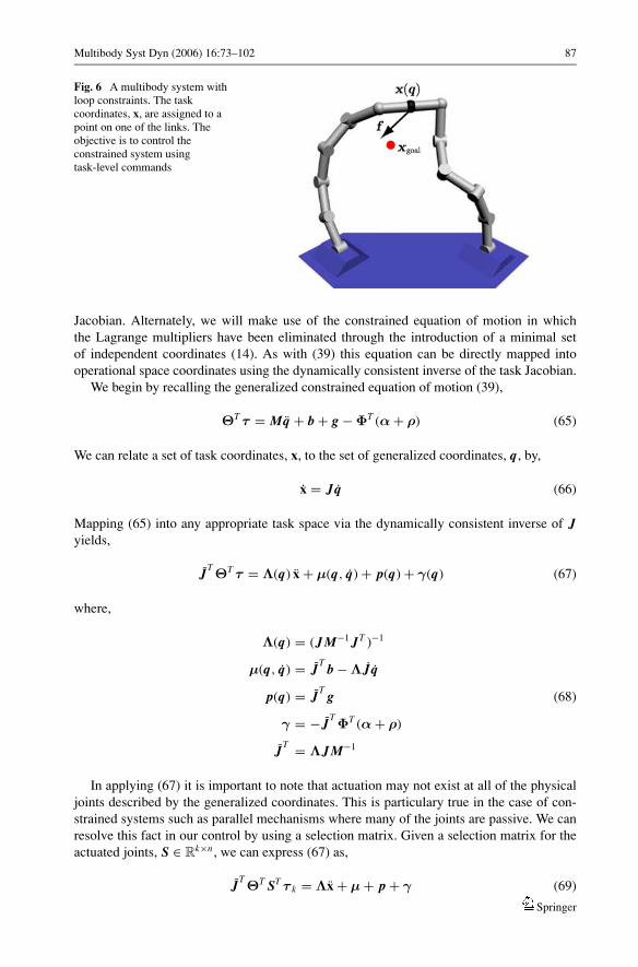
In previous work the control of constrained systems has been examined from a configurationspace perspective, particularly with regard to contact control in robot manipulators [26, 27].We will present an operational space methodology for addressing constrained systems, thusproviding a means of applying operational space control structures to these systems (seeFigure 6).

5.1. Direct task space mapping of constrained dynamics

This formulation involves directly mapping the generalized constrained equation of motion(39) into operational space coordinates using the dynamically consistent inverse of the task

Springer


Fig. 6 A multibody system withloop constraints. The taskcoordinates, x, are assigned to apoint on one of the links. Theobjective is to control theconstrained system usingtask-level commands

Jacobian. Alternately, we will make use of the constrained equation of motion in whichthe Lagrange multipliers have been eliminated through the introduction of a minimal setof independent coordinates (14). As with (39) this equation can be directly mapped intooperational space coordinates using the dynamically consistent inverse of the task Jacobian.

We begin by recalling the generalized constrained equation of motion (39),

ΘT τ = Mq + b + g − ΦT (α + ρ) (65)

We can relate a set of task coordinates, x, to the set of generalized coordinates, q, by,

x = Jq (66)

Mapping (65) into any appropriate task space via the dynamically consistent inverse of J

yields,

JT ΘT τ = Λ(q) x + μ(q, q) + p(q) + γ(q) (67)

where,

Λ(q) = (J M−1 JT )−1

μ(q, q) = JT

b − Λ Jq

p(q) = JT

g (68)

γ = − JT ΦT (α + ρ)

JT = ΛJ M−1

In applying (67) it is important to note that actuation may not exist at all of the physicaljoints described by the generalized coordinates. This is particulary true in the case of con-strained systems such as parallel mechanisms where many of the joints are passive. We canresolve this fact in our control by using a selection matrix. Given a selection matrix for theactuated joints, S ∈ Rk×n , we can express (67) as,

JT ΘT ST τ k = Λx + μ + p + γ (69)

Springer


where τ = ST τ k , and τ k is the k × 1 vector of generalized forces acting at the k actuatedjoints. The matrix J

T ΘT ST has dimensions of mT × k. Thus, k ≥ mT is a necessary conditionfor the system to yield a solution of τ k for an arbitrary acceleration, x.

In practice we can design task motion control using estimates of the operational spacedynamic properties. This yields the following dynamic compensation equation,

JT ΘT ST τ k = Λ f � + μ + p + γ (70)

where f � is the input of the decoupled system and we use the notation to represent estimatesof various quantities. Any suitable control law can be chosen to serve as this input. Inparticular, we can choose a linear control law of the form,

f � = Kp(xd − x) + K v(xd − x) + xd (71)

The procedure applied to (39) can also be applied to (14). In this case, however, the taskspace mapping is associated with the minimal set of generalized coordinates, qC . We beginby recalling (14),

τp = Mp(q) q p + bp(q, q p) + g p(q) (72)

We can relate a set of task coordinates, x, to the coordinates, q p, by,

x = Jq = Jp (q) q p (73)

where,

Jp (q) = JC (74)

is the task Jacobian with respect to the minimal set of coordinates. We can map (72) into anyappropriate task space via the dynamically consistent inverse of Jp. This yields [31],

f = Λ(q) x + μ(q, q p) + p(q) (75)

where,

Λ(q) = (Jp M−1

p JTp

)−1

μ(q, q p) = JTp bp − Λ Jp q p

(76)p(q) = J

Tp g p

JTp = ΛJp M−1

p

We can express (75) in terms of the generalized forces,

Jpτp = JpCT τ = Λx + μ + p (77)

Springer


Given a selection matrix for the actuated joints, S ∈ Rk×n , we can express (77) as,

JTp CT ST τ k = Λx + μ + p (78)

where τ p = CT τ = CT ST τ k . The matrix JpCT ST has dimensions of mT × k. Again,k ≥ mT is a necessary condition for the system to yield a solution of τ k for an arbitraryacceleration, x.

Using estimates of the operational space dynamic properties we have the following dy-namic compensation equation,

JTp CT ST τ k = Λ f � + μ + p (79)

where f � can be given by (71).

5.2. Task/constraint partitioning of dynamics

In this formulation the multiplier form of the constrained equation of motion (7) is mapped intooperational space using the dynamically consistent inverse of a Jacobian which characterizesboth task and constraints [8]. The resulting operational space equation is then partitionedinto an equation corresponding to task motion control, and an equation corresponding toconstraint forces.

We begin by recalling the multiplier form of the constrained equation of motion (7),

τ + ΦTλ = Mq + b + g (80)

Again, we can relate a set of task coordinates, x, to the set of generalized coordinates, q , by,

x = J q (81)

in addition to the constraint condition,

φ = Φq = 0 (82)

We can concatenate (81) and (82) into a single vector,

˙x =(

x

φ

)=

(J

Φ

)q = Jq (83)

where we use the notation ˇ to represent a quantity that is formed from the composition oftask and constraint terms.

The active generalized force can be decomposed into a task space component and a nullspace component as in (47),

τ = JT

f + NTτ o = (

JT ΦT ) (f

f C

)+ N

Tτ o (84)

Springer


where f C is the component of the applied operational space force acting along the constraintdirection. Equation (80) can thus be written as,

JT

(f

f C

)+ N

Tτ o + J

T(

0

λ

)= Mq + b + g (85)

We can now map (85) into operational space using the dynamically consistent inverse of J.This yields, (

f

f C

)+

(0

λ

)= Λ(q)

(x

0

)+ μ(q, q) + p(q) (86)

where the constraint condition, φ = 0, has been imposed. We have the following definitions,

Λ(q) �(

J M−1 JT J M−1ΦT

ΦM−1 JT ΦM−1ΦT

)−1

μ(q, q) � Λ

(J M−1b − Jq

ΦM−1b − Φq

)(87)

p(q) � Λ

(J M−1g

ΦM−1g

)

While (86) expresses the combined task-constraint dynamics of our system it is useful topartition the dynamics in the following manner,(

f

f C

)+

(0

λ

)=

(Λ11 Λ12

Λ21 Λ22

) (x

0

)+

(μ1

μ2

)+

(p1

p2

)(88)

From this partitioning we have an equation corresponding to task motion control,

f = Λ11x + μ1 + p1 (89)

and an equation corresponding to constraint forces,

f C + λ = Λ21x + μ2 + p2 (90)

The constraint force vector, λ, will always arise so as to satisfy (90), as dictated by con-straint consistency. The component of applied operational space force, f C , acting along theconstraint direction has no impact on the motion control of the task. Its only effect is on theconstraint forces (values of λ) that arise. Thus, all choices for f C result in equivalent motioncontrol of the system [16]. However, specific choices can be made to optimize the controlwith regard to desired constraint forces or to account for certain joints being unactuated. Asan example of the latter case we may impose the condition that certain joints are unactuated.The following condition expresses the absence of actuation at those joints,

S(JT f + ΦT f C ) = 0 (91)

Springer


Fig. 7 An operational spacetracking controller for aconstrained system. The desiredtask is tracked using appropriatedynamic compensation whichaccounts for the constraints. Theterms τ o and f C are chosen aspart of the overall control design.An active applied torque isdelivered to the plant

where S ∈ R(n−k)×n is a selection matrix for the unactuated joints. That is, S selects the unac-tuated joints from the overall generalized force vector. Equation (91) would thus complement(89) and (90).

Using estimates of the operational space dynamic properties we have the following dy-namic compensation equation,

f = ˆΛ11 f � + ˆμ1 + ˆp1 (92)

where f � can be given by (71). The constraint force control term, f C , can be resolved byusing,

f C + λ = ˆΛ21 f � + ˆμ2 + ˆp2 (93)

in the case that the control is chosen with regard to optimizing the resulting constraint forces,or, by using (91) in order to account for certain joints being unactuated. Figure 7 depictsan operational space tracking controller for a constrained system based on this partitioningapproach.

5.3. Conditions on motion control

Figure 8 illustrates the necessary conditions for fully controlling the multibody system withrespect to the system degrees of freedom and the task coordinates. For the system to be motionactuated the number of actuators must equal or exceed the number of degrees of freedom, p.For the system to be task actuated the number of actuators must equal or exceed the numberof task coordinates, mT .

There are other conditions in addition to those stated above. Regarding task actuation,in the first formulation of Section 5.1 the matrix J

T ΘT ST must be full rank. Similarly, inthe second formulation of Section 5.1 the matrix JpCT ST must be full rank. Finally, in theformulation of Section 5.2 the matrix SΦT must be full rank.

Springer


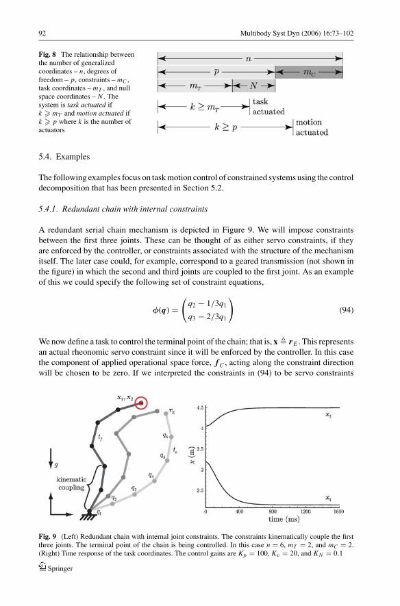
Fig. 8 The relationship betweenthe number of generalizedcoordinates – n, degrees offreedom – p, constraints – mC ,task coordinates – mT , and nullspace coordinates – N . Thesystem is task actuated ifk � mT and motion actuated ifk � p where k is the number ofactuators

5.4. Examples

The following examples focus on task motion control of constrained systems using the controldecomposition that has been presented in Section 5.2.

5.4.1. Redundant chain with internal constraints

A redundant serial chain mechanism is depicted in Figure 9. We will impose constraintsbetween the first three joints. These can be thought of as either servo constraints, if theyare enforced by the controller, or constraints associated with the structure of the mechanismitself. The later case could, for example, correspond to a geared transmission (not shown inthe figure) in which the second and third joints are coupled to the first joint. As an exampleof this we could specify the following set of constraint equations,

φ(q) =(

q2 − 1/3q1

q3 − 2/3q1

)(94)

We now define a task to control the terminal point of the chain; that is, x � r E . This representsan actual rheonomic servo constraint since it will be enforced by the controller. In this casethe component of applied operational space force, f C , acting along the constraint directionwill be chosen to be zero. If we interpreted the constraints in (94) to be servo constraints

Fig. 9 (Left) Redundant chain with internal joint constraints. The constraints kinematically couple the firstthree joints. The terminal point of the chain is being controlled. In this case n = 6, mT = 2, and mC = 2.(Right) Time response of the task coordinates. The control gains are Kp = 100, Kv = 20, and KN = 0.1

Springer


Fig. 10 (Left) Time response of first three joints for the constrained redundant chain. Constraints are enforcedconsistent with (94). (Right) The 2-dimensional null space is being controlled to minimize gravity effort,

U = ‖g(q)‖2. The null space term, −KN NT ∇U , executes a task and constraint consistent minimization

they would be incorporated into x rather then φ. This would change the control torques sincethe constraints would be enforced by the controller rather than the internal structure of themechanism.

The 2-dimensional null space is controlled to minimize the gravity effort, defined asU � ‖g(q)‖2. Our control torque is then,

τ = JT f − KN NT ∂U

∂q(95)

where f is given by (92) and KN is a null space gain. All joints are assumed to be actuatedso no selection matrix needs to be introduced. Simulation plots for the system under a goalposition command are shown in Figures 9 and 10. A linear (PD) control law is used as theinput of the decoupled system (71). A small amount of damping was applied in the nullspace to damp out oscillations. In Figure 10 we note that the gravity effort is minimized in amanner consistent with the task and constraints. We also see that the time histories of the firstthree joint torques exhibit some spikes due to the rapid and drastic changes in configurationinduced by the gravity effort minimization.

5.4.2. Mechanism with loop closures

A parallel mechanism is depicted in Figure 11. The constraint equations describe the loopclosures and are given by,

φ(q) =⎛⎝ r p1 − r l1

r p2 − r l2

r p3 − r l3

⎞⎠ (96)

The task is defined to control the active elbow joints; that is, x � ( q2 q4 q6 )T . Thiscorresponds to,

J =

⎛⎜⎝ 0 1 0 0 0 0 0 0 0

0 0 0 1 0 0 0 0 0

0 0 0 0 0 1 0 0 0

⎞⎟⎠ (97)

Springer


Fig. 11 (Left) Parallel mechanism consisting of serial chains with loop closures. The three elbow joints areactively controlled while the remaining joints are passive. (Right) The orientation of the platform is commandedto rotate while its center is to remain fixed. In this case n = 9, mT = 3, mC = 6, and k = 3

Due to the passive nature of all other joints the component of active force, f C , acting alongthe constraint direction is chosen to be zero. This can be derived from the condition of (91),where,

S =

⎛⎜⎜⎜⎜⎜⎜⎜⎜⎝

1 0 0 0 0 0 0 0 0

0 0 1 0 0 0 0 0 0

0 0 0 0 1 0 0 0 0

0 0 0 0 0 0 1 0 0

0 0 0 0 0 0 0 1 0

0 0 0 0 0 0 0 0 1

⎞⎟⎟⎟⎟⎟⎟⎟⎟⎠(98)

Since SJT f = 0,

f C = −(SΦT )−1 SJT f = 0 (99)

There is no null space in this particular example so our control torque is given by τ = JT f ,where f is given by (92). Figure 12 shows simulation plots for the system under a goal positioncommand. A linear (PD) control law is used as the input of the decoupled system.

In a second case we will define the task to control the position and orientation of theplatform (see Figure 11); that is, x � ( q7 q8 q9 )T . In this case f C = 0 since SJT f = 0.The orientation is commanded to rotate while the center of the platform is commanded toremain fixed. A linear (PD) control law is used as the input of the decoupled system. Figure13 shows simulation plots for the system under a goal position command.

5.4.3. Underactuated redundant chain

A redundant serial chain with an unactuated joint is depicted in Figure 14. The task is definedto control the terminal point of the chain, that is x � r E . Since the number of actuators,k = 2, is less the number of degrees of freedom, p = 3, the system is under-actuated with

Springer


Fig. 12 (Left) Time response of the elbow joints moving to a goal. (Right) Time response of the controltorques during goal movement. Zero control torque is produced at the passive joints. The control gains areKp = 100 and Kv = 20

Fig. 13 The orientation of the platform is commanded to rotate while its center is to remain fixed. (Left) Timeresponse of the platform orientation. (Right) Time response of the control torques during goal movement.Zero control torque is produced at the passive joints. The control gains are Kp = 100 and Kv = 20

Fig. 14 (Left) Under-actuated redundant chain. Joint 1 is unactuated (passive). In this case n = 3, k = 2,and mT = 2. (Right) Time response of the task coordinates for the under-actuated system moving to a goallocation. The control gains are Kp = 100 and Kv = 20

Springer


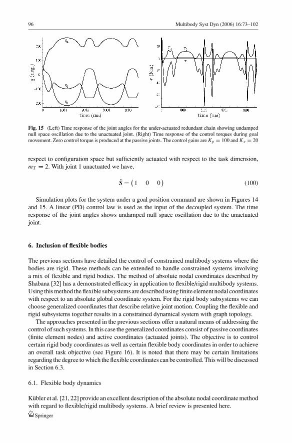
Fig. 15 (Left) Time response of the joint angles for the under-actuated redundant chain showing undampednull space oscillation due to the unactuated joint. (Right) Time response of the control torques during goalmovement. Zero control torque is produced at the passive joints. The control gains are Kp = 100 and Kv = 20

respect to configuration space but sufficiently actuated with respect to the task dimension,mT = 2. With joint 1 unactuated we have,

S = (1 0 0

)(100)

Simulation plots for the system under a goal position command are shown in Figures 14and 15. A linear (PD) control law is used as the input of the decoupled system. The timeresponse of the joint angles shows undamped null space oscillation due to the unactuatedjoint.

6. Inclusion of flexible bodies

The previous sections have detailed the control of constrained multibody systems where thebodies are rigid. These methods can be extended to handle constrained systems involvinga mix of flexible and rigid bodies. The method of absolute nodal coordinates described byShabana [32] has a demonstrated efficacy in application to flexible/rigid multibody systems.Using this method the flexible subsystems are described using finite element nodal coordinateswith respect to an absolute global coordinate system. For the rigid body subsystems we canchoose generalized coordinates that describe relative joint motion. Coupling the flexible andrigid subsystems together results in a constrained dynamical system with graph topology.

The approaches presented in the previous sections offer a natural means of addressing thecontrol of such systems. In this case the generalized coordinates consist of passive coordinates(finite element nodes) and active coordinates (actuated joints). The objective is to controlcertain rigid body coordinates as well as certain flexible body coordinates in order to achievean overall task objective (see Figure 16). It is noted that there may be certain limitationsregarding the degree to which the flexible coordinates can be controlled. This will be discussedin Section 6.3.

6.1. Flexible body dynamics

Kubler et al. [21, 22] provide an excellent description of the absolute nodal coordinate methodwith regard to flexible/rigid multibody systems. A brief review is presented here.

Springer


Fig. 16 A rigid/flexiblemultibody system withconstraints between the bodies. Aset of nodal displacements areassigned as the task coordinates

Fig. 17 Isoparametric elements showing the mapping from the intrinsic parameter space, ξ, to the physicalspace, X. (Top) An 8 node hexahedral element (Bottom) A higher order 27 node hexahedral element

For a given flexible body subsystem a Lagrangian or material description is chosen whichrelates all quantities to the reference configuration, X, of the system with domain �o. Usinga nonlinear finite element approach a set of shape or interpolating functions, {N1, . . . , Ns},associated with a particular finite element discretization of s nodes can be chosen.

In the case of 8 node isoparametric hexahedral elements (see Figure 17) the interpolatingfunctions are given as [15],

Na(ξ) = 1

8(1 + ξaξ ) (1 + ηaη) (1 + ζaζ ) for a = 1, 2, . . . , 8 (101)

Springer


where ξ = ( ξ η ζ )T are the coordinates of the intrinsic element parameter space. For thehigher order 27 node hexahedral element, Lagrange polynomials can be used to constructthe interpolating functions [15]. Defining the shape matrix, N ∈ R3×3s ,

N �

⎛⎜⎝ N1 0 0 · · · Ns 0 0

0 N1 0 · · · 0 Ns 0

0 0 N1 · · · 0 0 Ns

⎞⎟⎠ (102)

the displacement field, u(X, t) ∈ R3, is given by u = Nd, where d ∈ R3s is the vector of nodaldisplacements. The current material configuration is then given by x(X, t) = X + u(X, t).The weak form statement (summation convention applied) of the elastodynamics problemis,

δd j (Mjkdk + k j + g j ) = 0 (103)

where,

Mjk =∫

�o

ρo Ni j NikdV

k j =∫

�o

∂ Ni j

∂ Xk

(δil + ∂ Nil

∂ Xkdk

)SlkdV

g j = −∫

�o

ρo Ni j bi dV −∫

∂�o

Ni j pi d A (104)

The term ρo is the material density field in the reference configuration, bi are the body forces(eg. gravity), pi are the surface forces, δil is the Kronecker delta, and Slk is the secondPiola-Kirchoff stress tensor. The system can thus be stated as,

Md + k + g = 0 (105)

or more generally as,

Md + k + g = f (106)

where f ∈ R3s is a vector of external control forces applied at the nodes. The termsM ∈ R3s×3s , k ∈ R3s , and g ∈ R3s are the mass matrix, stiffness vector, and body/surfaceforce vector respectively. It is noted that due to integration with respect to the referenceconfiguration, �o, the mass matrix, M, is constant. The stress tensor, S, is highly nonlinearhowever.

Different constitutive models can be applied. In particular, viscous effects are importantfor some systems. Structural damping models are discussed in [22], however we will notconsider these detailed constitutive models since it is assumed that the basic mathematicalstructure of (106) can still be achieved with these models. For the remainder of this sectionwe will focus on the mathematical structure of (106) rather than the constitutive specifics ofthe terms.

Springer


6.2. Subsystem assembly

We can assemble a set of rigid and flexible subsystems into single constrained system. First,we specify the dynamics of a set of y unconstrained rigid body subsystems,

τ 1 = Mr1 q1 + b1 + gr1

...

τ y = Mry q y + by + gry

(107)

Next, we specify the dynamics of a set of z flexible subsystems which have been discretizedusing absolute nodal coordinates,

f 1 = Mf1 d1 + k1 + g f1

...

f z = Mfz d z + kz + g fz

(108)

The sets of equations given by (107) and (108) can be assembled into a single system equationof the form,

τ = Mq + b + g (109)

where,

M = diag(Mr1 , · · · , Mry , Mf1 , · · · , Mfz

)τ = (

τ T1 · · · τ T

y f T1 · · · f T

z

)T

q = (qT

1 · · · qTy d

T1 · · · d

Tz

)T(110)

b = (bT

1 · · · bTy kT

1 · · · kTz

)T

g = (gT

r1· · · gT

rygT

f1· · · gT

fz

)T

We have M ∈ Rn×n and τ , q, b, g ∈ Rn where,

n =y∑

i=1

nri +z∑

i=1

nfi

nfi = 3si

(111)

Springer


Imposing a set of mC holonomic constraint equations to establish system connectivity yieldsthe familiar equation,

τ = Mq + b + g − ΦTλ (112)

subject to,

Φq + Φq = 0 (113)

6.3. Control issues

We can apply the same control methodology to the constrained flexible/rigid multibodysystem described in Section 6.2 that was applied to the constrained rigid multibody systemaddressed earlier in this paper. A number of issues need to be recognized however. Typically,flexible body subsystems will be passive. That is, there will be no control forces, f , appliedat the nodes. While a selection matrix, S, can be used to specify the actuated coordinates, therank conditions given in Section 5.3 must still be satisfied (in addition to the condition on thenumber of actuators) to control the task nodal coordinates. Satisfying these rank conditions isproblematic because the nodes in the flexible body subsystems are not kinematically coupled,as the bodies in the rigid body subsystems are, but rather elastically coupled. Sparseness ofthe mass matrices and task Jacobians of the flexible body subsystems is a consequence ofthis lack of kinematic coupling.

In rigid body systems, kinematic coupling allows a desired acceleration at the task controlpoint to be achieved despite the lack of actuation at certain joints. This can be realized byrecalling (69),

JT ΘT ST τ k = Λx + μ + p + γ (114)

The matrix JT ΘT ST must be full rank for there to be solution of actuator generalized forces to

achieve an arbitrary task acceleration, x. Kinematic coupling results in a dense task Jacobianand mass matrix, whereas elastic coupling in flexible systems results in a sparse task Jacobianand mass matrix. In this case, if the actuated nodal coordinates do not correspond to the nodalcoordinates that constitute the task then the term J

T ΘT ST will be rank deficient. While thisfact precludes finding a control input to achieve the desired task nodal accelerations at agiven instant, control inputs may still exist that achieve the desired task nodal displacementsin static equilibrium.

An additional consideration is that the task nodal displacements will typically be comprisedof large rigid body displacements and small material deformations. As a practical matter ifthe specified desired nodal displacements involve large deformations the elastic forces willbe large and the corresponding control input will be prohibitively large, particularly for stiffmaterials. Finally, it should be emphasized that applying this in an actual control system fora flexible/rigid multibody system requires sensing at the nodes of the flexible bodies.

7. Summary and conclusions

In this paper we have presented a task-level methodology for the control of constrainedmultibody systems. This methodology exploits the natural symmetry between constrained

Springer


dynamics and task space dynamics to synthesize dynamic compensation which properlyaccounts for the system constraints while performing a control task. The presence of passivejoints in the constrained system has also been accommodated. A set of examples demonstratedthe efficacy of this methodology in simulation. As a practical matter it is assumed that thecontroller has access to the system state (via a forward dynamics solver in the simulated caseor via sensors in the physical case) and estimates of the dynamic properties of the physicalsystem.

Application to flexible/rigid multibody systems was also addressed. The absolute nodalcoordinate method can be used to describe the flexible bodies in conjunction with generalizedcoordinates that describe relative joint motion for the rigid bodies. A standard assemblyprocedure can be employed and connectivity constraints imposed to form a constrainedflexible/rigid multibody system. The task-level control approaches presented here can thenbe applied in the same manner as with constrained rigid multibody systems. Since the nodesdescribing a flexible body are typically passive and elastically coupled there are limitationsin controlling flexible body nodes as part of the task however. This is in contrast to passivejoints between kinematically coupled rigid bodies.

The task-level constraint based control methods addressed here can be applied to mo-tion control which involves contact with the environment. A particular application area forthis is locomotion in robotic systems. The contact kinematics associated with intermittentfoot/ground contact during gait can be modeled using constraints, as was done by Schiehlen[33]. The robot controller can thus employ a constraint based approach where transitionsbetween different contact conditions can be detected and accommodated. This approach isapplicable to a host of tasks outside of locomotion and represents a general methodology forconstrained motion control.

Acknowledgments Support for this work was provided by NIH V54GM072970, HD33929, and HD046814.The authors would like to thank Katherine Holzbaur for providing a motivation for this work with regard toconstrained biomechanical systems. The helpful comments provided by Jaeheung Park and James Warren arealso appreciated. Vincent De Sapio would like to thank Sandia National Laboratories for supporting this work.

References

1. Bajodah, A.H., Hodges, D.H., Chen, Y.: Inverse dynamics of servo-constraints based on the generalizedinverse. Nonlinear Dynamics 39, 179–196 (2005)

2. Blajer, W.: A geometric unification of constrained system dynamics. Multibody System Dynamics 1, 3–21(1997)

3. Blajer, W., Kolodziejczyk, K.: A geometric approach to solving problems of control constraints: theoryand a DAE framework. Multibody System Dynamics 11, 343–364 (2004)

4. Bruyninckx, H., Khatib, O.: Gauss’ principle and the dynamics of redundant and constrained manipulators.In Proceedings of the 2000 IEEE International Conference on Robotics and Automation, 3, 2563–2568.San Francisco, April (2000)

5. Chang, K.-S., Holmberg, R., Khatib, O.: The augmented object model: Cooperative manipulation andparallel mechanism dynamics. In Proceedings of the 2000 IEEE International Conference on Roboticsand Automation 1, 470–475, San Francisco, April (2000)

6. Craig, J.J.: Introduction to robotics: mechanics and control, 3rd ed., Upper Saddle River NJ: Prentice Hall(2004)

7. De Sapio, V.: Some approaches for modeling and analysis of a parallel mechanism with stewart platformarchitecture. In Proceedings of the 1998 ASME International Mechanical Engineering Congress andExposition MED-8, 637–649, Anaheim CA, November 7, (1998)

8. De Sapio, V., Khatib, O.: Operational space control of multibody systems with explicit holonomic con-straints. In Proceedings of the 2005 IEEE International Conference on Robotics and Automation 1,470–475, Barcelona, April (2005)

Springer


9. Delp, S.L., Loan, J.P., Hoy, M.G., Zajac, F.E., Topp, E.L., Rosen, J.M.: An interactive graphics-basedmodel of the lower extremity to study orthopaedic surgical procedures. IEEE Transactions on BiomedicalEngineering 37, 757–767 (1990)

10. Featherstone, R.: Robot Dynamics Algorithms, 1st ed., New York: Kluwer (1987)11. Gauss, K.F.: Uber ein neues allgemeines Grundgesetz der Mechanik (On a New Fundamental Law of

Mechanics). Journal fur die Reine und Angewandte Mathematik 4, 232–235 (1829)12. Gibbs, J.W.: On the funfamental formulae of dynamics. American Journal of Mathematics 2, 49–64 (1879)13. Harary, F.: Graph Theory, 1st ed., Reading MA: Perseus (1969)14. Holzbaur, K.R.S., Murray, W.M., Delp, S.L.: A model of the upper extremity for simulating musculoskele-

tal surgery and analyzing neuromuscular control. Annals of Biomedical Engineering 33(6), 829–840(2005)

15. Hughes, T.J.R.: The finite element method: linear static and dynamic finite element analysis, reprint, NewYork: Dover (2000)

16. Huston, R.L., Liu, C.Q., Li, F.: Equivalent control of constrained multibody systems. Multibody SystemDynamics 10(3), 313–321 October (2003)

17. Jungnickel, U.: Differential-algebraic equations in riemannian spaces and applications to multibody systemdynamics. ZAMM 74(9), 409–415 (1994)

18. Kane, T., Levinson, D.: Dynamics: theory and applications. 1st ed., New York: McGraw-Hill (1985)19. Khatib, O.: A unified approach to motion and force control of robot manipulators: the operational space

formulation. International Journal of Robotics Research 3(1), 43–53 (1987)20. Khatib, O.: Inertial properties in robotic manipulation: an object level framework. International Journal

of Robotics Research 14(1), 19–36 February (1995)21. Kubler, L., Eberhard, P., Geisler, J.: Flexible multibody systems with large deformations using absolute

nodal coordinates for isoparametric solid brick elements. In Proceedings of the 2003 ASME DesignEngineering Technical Conference September (2003)

22. Kubler, L., Eberhard, P., Geisler, J.: Flexible multibody systems with large deformations and nonlinearstructural damping using absolute nodal coordinates. Nonlinear Dynamics, 34(1–2), 31–52 (2003)

23. Lanczos, C.: The variational principles of mechanics. 4th ed., New York: Dover (1986)24. Lenarcic, J., Stanisic, M.M.: A humanoid shoulder complex and the humeral pointing kinematics. IEEE

Transactions on Robotics and Automation 19(3), 499–506 June (2003)25. Lilly, K.W.: Efficient dynamic simulation of robotic mechanisms, 1st ed., Boston: Kluwer (1993)26. Liu, Y.-H., Arimoto, S., Kitagaki, K.: Adaptive control for holonomically constrained robots: time-invariant

and time-variant cases. In Proceedings of the 1995 IEEE International Conference on Robotics andAutomation 1, 905–912, Nagoya, Japan May (1995)

27. Liu, Y.-H., Kitagaki, K., Ogasawara, T., Arimoto, S.: Model-based adaptive hybrid control for manipulatorsunder multiple geometric constraints . IEEE Transactions on Robotics and Automation 7(1), 97–109January (1999)

28. Moon, F.: Applied dynamics. 1st ed., New York: John Wiley and Sons (1998)29. Papastavridis, J.G.: Analytical mechanics: A comprehensive treatise on the dynamics of constrained

systems for engineers. Physicists, and Mathematicians, Oxford university Press (2002)30. Pars, L.A.: A Treatise on Analytical Dynamics. reprint, Woodbridge CT: Ox Bow Press (1979)31. Russakow, J., Khatib, O., Rock, S.M.: Extended operational space formulation for serial-to-parallel chain

(branching) manipulators. In Proceedings of the the 1995 IEEE International Conference on Robotics andAutomation 1, 1056–1061, Nagoya, Japan, May (1995)

32. Shabana, A.: Computer implementation of the absolute nodal coordinate formulation for flexible multibodydynamics. Nonlinear Dynamics 16(3), 293–306 July (1998)

33. Schiehlen, W.: Energy-optimal design of walking machines. Multibody System Dynamics 13(1), 129–141February (2005)

34. Udwadia, F.E., Kalaba, R.E.: Analytical dynamics: a new approach. 1st ed., Cambridge: CambridgeUinversity Press (1996)

35. von Schwerin, R.: Multibody system simulation. 1st ed., Berlin: Springer (1999)36. Wehage, R.A., Haug, E.J.: Generalized coordinate partitioning for dimension reduction in analysis of

constrained dynamic systems. Journal of Mechanical Design 104(1), 247–255 (1982)

Springer

Documents

Task-level approaches for the control of constrained ...nmbl.stanford.edu/publications/pdf/Desapio2006.pdf · Springer ScienceC +Business Media B.V. 2006 Abstract This paper presents