Embed Size (px)
Citation preview
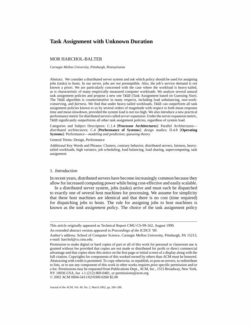
Task Assignment with Unknown Duration
MOR HARCHOL-BALTER
Carnegie Mellon University, Pittsburgh, Pennsylvania
Abstract. We consider a distributed server system and ask which policy should be used for assigningjobs (tasks) to hosts. In our server, jobs arenot preemptible. Also, the job’s service demand isnotknown a priori. We are particularly concerned with the case where the workload is heavy-tailed,as is characteristic of many empirically measured computer workloads. We analyze several naturaltask assignment policies and propose a new oneTAGS (Task Assignment based on Guessing Size).The TAGS algorithm is counterintuitive in many respects, including loadunbalancing,non-work-conserving, andfairness. We find that under heavy-tailed workloads,TAGS can outperform all taskassignment policies known to us by several orders of magnitude with respect to both mean responsetime and mean slowdown, provided the system load is not too high. We also introduce a new practicalperformance metric for distributed servers calledserver expansion. Under the server expansion metric,TAGS significantly outperforms all other task assignment policies, regardless of system load.
Categories and Subject Descriptors: C.1.4 [Processor Architectures]: Parallel Architectures—distributed architectures; C.4 [Performance of Systems]: design studies; D.4.8 [OperatingSystems]: Performance—modeling and prediction; queueing theory
General Terms: Design, Performance
Additional Key Words and Phrases: Clusters, contrary behavior, distributed servers, fairness, heavy-tailed workloads, high variance, job scheduling, load balancing, load sharing, supercomputing, taskassignment
1. Introduction
In recent years, distributed servers have become increasingly common because theyallow for increased computing power while being cost-effective and easily scalable.
In a distributed server system, jobs (tasks) arrive and must each be dispatchedto exactly one of several host machines for processing. We assume for simplicitythat these host machines are identical and that there is no cost (time required)for dispatching jobs to hosts. The rule for assigning jobs to host machines isknown as thetask assignment policy. The choice of the task assignment policy
This article originally appeared as Technical Report CMU-CS-99-162, August 1999.An extended abstract version appeared inProceedings of the ICDCS ’00.Author’s address: School of Computer Science, Carnegie Mellon University, Pittsburgh, PA 15213,e-mail: [email protected] to make digital or hard copies of part or all of this work for personal or classroom use isgranted without fee provided that copies are not made or distributed for profit or direct commercialadvantage and that copies show this notice on the first page or initial screen of a display along with thefull citation. Copyrights for components of this worked owned by others than ACM must be honored.Abstracting with credit is permitted. To copy otherwise, to republish, to post on servers, to redistributeto lists, or to use any component of this work in other works requires prior specific permission and/ora fee. Permissions may be requested from Publications Dept., ACM, Inc., 1515 Broadway, New York,NY 10036 USA, fax+1 (212) 869-0481, or [email protected]© 2002 ACM 0004-5411/02/0300-0260 $5.00
Journal of the ACM, Vol. 49, No. 2, March 2002, pp. 260–288.
Task Assignment with Unknown Duration 261
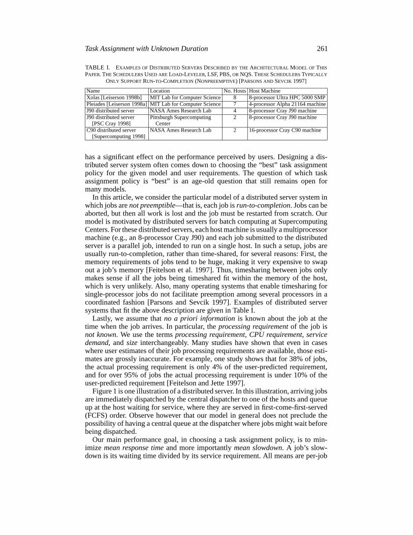
TABLE I. EXAMPLES OFDISTRIBUTED SERVERSDESCRIBED BY THEARCHITECTURAL MODEL OFTHIS
PAPER. THE SCHEDULERSUSED ARELOAD-LEVELER, LSF, PBS,OR NQS. THESESCHEDULERSTYPICALLY
ONLY SUPPORTRUN-TO-COMPLETION (NONPREEMPTIVE) [PARSONS ANDSEVCIK 1997]
Name Location No. Hosts Host MachineXolas [Leiserson 1998b] MIT Lab for Computer Science 8 8-processor Ultra HPC 5000 SMPPleiades [Leiserson 1998a]MIT Lab for Computer Science 7 4-processor Alpha 21164 machineJ90 distributed server NASA Ames Research Lab 4 8-processor Cray J90 machineJ90 distributed server Pittsburgh Supercomputing 2 8-processor Cray J90 machine
[PSC Cray 1998] CenterC90 distributed server NASA Ames Research Lab 2 16-processor Cray C90 machine
[Supercomputing 1998]
has a significant effect on the performance perceived by users. Designing a dis-tributed server system often comes down to choosing the “best” task assignmentpolicy for the given model and user requirements. The question of which taskassignment policy is “best” is an age-old question that still remains open formany models.
In this article, we consider the particular model of a distributed server system inwhich jobs arenot preemptible—that is, each job isrun-to-completion. Jobs can beaborted, but then all work is lost and the job must be restarted from scratch. Ourmodel is motivated by distributed servers for batch computing at SupercomputingCenters. For these distributed servers, each host machine is usually a multiprocessormachine (e.g., an 8-processor Cray J90) and each job submitted to the distributedserver is a parallel job, intended to run on a single host. In such a setup, jobs areusually run-to-completion, rather than time-shared, for several reasons: First, thememory requirements of jobs tend to be huge, making it very expensive to swapout a job’s memory [Feitelson et al. 1997]. Thus, timesharing between jobs onlymakes sense if all the jobs being timeshared fit within the memory of the host,which is very unlikely. Also, many operating systems that enable timesharing forsingle-processor jobs do not facilitate preemption among several processors in acoordinated fashion [Parsons and Sevcik 1997]. Examples of distributed serversystems that fit the above description are given in Table I.
Lastly, we assume thatno a priori informationis known about the job at thetime when the job arrives. In particular, theprocessing requirementof the job isnot known. We use the termsprocessing requirement, CPU requirement, servicedemand, andsize interchangeably. Many studies have shown that even in caseswhere user estimates of their job processing requirements are available, those esti-mates are grossly inaccurate. For example, one study shows that for 38% of jobs,the actual processing requirement is only 4% of the user-predicted requirement,and for over 95% of jobs the actual processing requirement is under 10% of theuser-predicted requirement [Feitelson and Jette 1997].
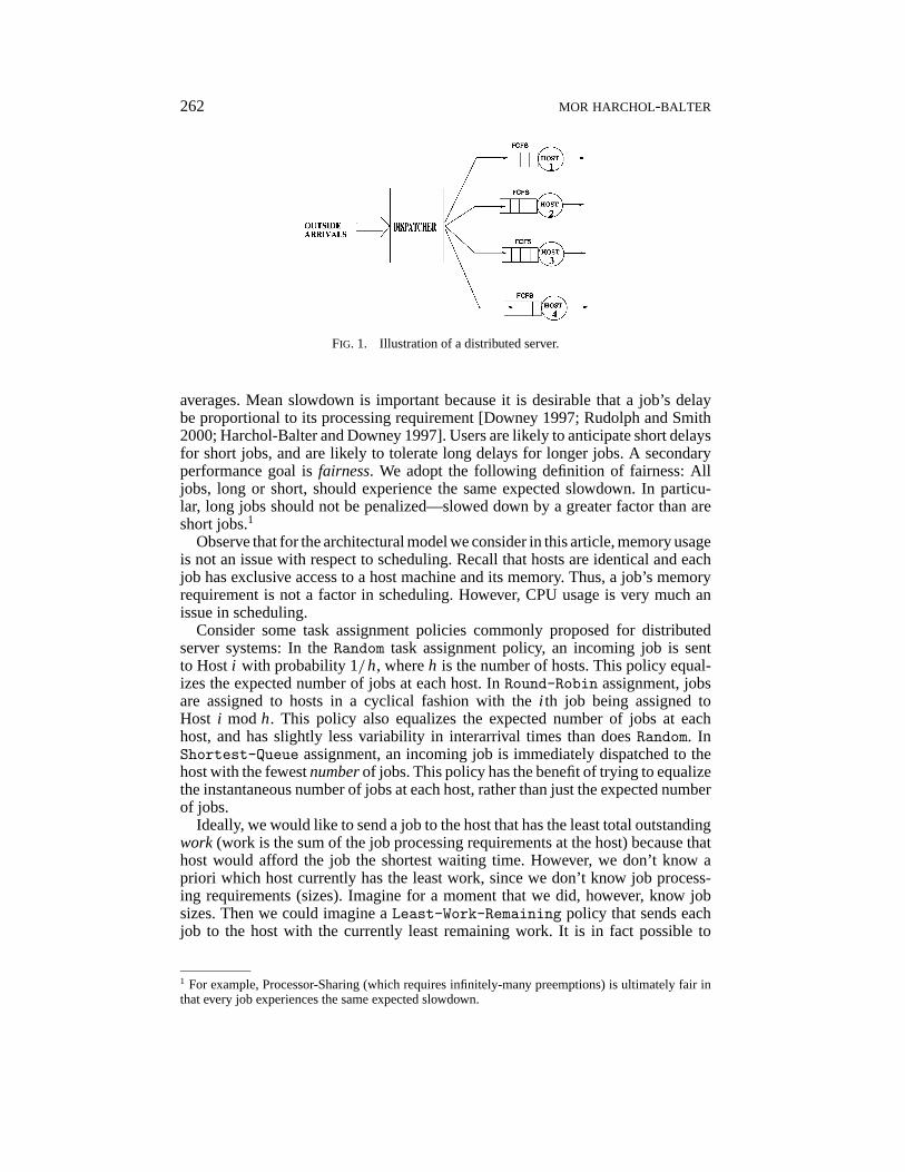
Figure 1 is one illustration of a distributed server. In this illustration, arriving jobsare immediately dispatched by the central dispatcher to one of the hosts and queueup at the host waiting for service, where they are served in first-come-first-served(FCFS) order. Observe however that our model in general does not preclude thepossibility of having a central queue at the dispatcher where jobs might wait beforebeing dispatched.
Our main performance goal, in choosing a task assignment policy, is to min-imize mean response timeand more importantlymean slowdown. A job’s slow-down is its waiting time divided by its service requirement. All means are per-job
262 MOR HARCHOL-BALTER
FIG. 1. Illustration of a distributed server.
averages. Mean slowdown is important because it is desirable that a job’s delaybe proportional to its processing requirement [Downey 1997; Rudolph and Smith2000; Harchol-Balter and Downey 1997]. Users are likely to anticipate short delaysfor short jobs, and are likely to tolerate long delays for longer jobs. A secondaryperformance goal isfairness. We adopt the following definition of fairness: Alljobs, long or short, should experience the same expected slowdown. In particu-lar, long jobs should not be penalized—slowed down by a greater factor than areshort jobs.1
Observe that for the architectural model we consider in this article, memory usageis not an issue with respect to scheduling. Recall that hosts are identical and eachjob has exclusive access to a host machine and its memory. Thus, a job’s memoryrequirement is not a factor in scheduling. However, CPU usage is very much anissue in scheduling.
Consider some task assignment policies commonly proposed for distributedserver systems: In theRandom task assignment policy, an incoming job is sentto Hosti with probability 1/h, whereh is the number of hosts. This policy equal-izes the expected number of jobs at each host. InRound-Robin assignment, jobsare assigned to hosts in a cyclical fashion with thei th job being assigned toHost i modh. This policy also equalizes the expected number of jobs at eachhost, and has slightly less variability in interarrival times than doesRandom. InShortest-Queue assignment, an incoming job is immediately dispatched to thehost with the fewestnumberof jobs. This policy has the benefit of trying to equalizethe instantaneous number of jobs at each host, rather than just the expected numberof jobs.
Ideally, we would like to send a job to the host that has the least total outstandingwork (work is the sum of the job processing requirements at the host) because thathost would afford the job the shortest waiting time. However, we don’t know apriori which host currently has the least work, since we don’t know job process-ing requirements (sizes). Imagine for a moment that we did, however, know jobsizes. Then we could imagine aLeast-Work-Remaining policy that sends eachjob to the host with the currently least remaining work. It is in fact possible to
1 For example, Processor-Sharing (which requires infinitely-many preemptions) is ultimately fair inthat every job experiences the same expected slowdown.
Task Assignment with Unknown Duration 263
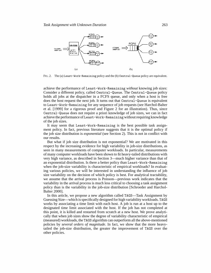
FIG. 2. The (a)Least-Work-Remaining policy and the (b)Central-Queue policy are equivalent.
achieve the performance ofLeast-Work-Remaining withoutknowing job sizes:Consider a different policy, calledCentral-Queue. TheCentral-Queue policyholds all jobs at the dispatcher in a FCFS queue, and only when a host is freedoes the host request the next job. It turns out thatCentral-Queue is equivalentto Least-Work-Remaining for any sequence of job requests (see Harchol-Balteret al. [1999] for a rigorous proof and Figure 2 for an illustration). Thus, sinceCentral-Queue does not require a priori knowledge of job sizes, we can in factachieve the performance ofLeast-Work-Remainingwithout requiring knowledgeof the job sizes.
It may seem thatLeast-Work-Remaining is the best possible task assign-ment policy. In fact, previous literature suggests that it is the optimal policy ifthe job size distribution isexponential(see Section 2). This is not in conflict withour results.
But what if job size distribution is not exponential? We are motivated in thisrespect by the increasing evidence for high variability in job-size distributions, asseen in many measurements of computer workloads. In particular, measurementsof many computer workloads have been shown to fit heavy-tailed distributions withvery high variance, as described in Section 3—much higher variance than that ofan exponential distribution. Is there a better policy thanLeast-Work-Remainingwhen the job-size variability is characteristic of empirical workloads? In evaluat-ing various policies, we will be interested in understanding the influence of jobsize variability on the decision of which policy is best. For analytical tractability,we assume that the arrival process is Poisson—previous work indicates that thevariability in the arrival process is much less critical to choosing a task assignmentpolicy than is the variability in the job-size distribution [Schroeder and Harchol-Balter 2000].
In this article, we propose a new algorithm calledTAGS—Task Assignment byGuessing Size—which is specifically designed for high variability workloads.TAGSworks by associating a time limit with each host. A job is run at a host up to thedesignated time limit associated with the host. If the job has not completed atthis point, it is killed and restarted from scratch at a new host. We prove analyti-cally that when job sizes show the degree of variability characteristic of empirical(measured) workloads, theTAGS algorithm can outperform all the above-mentionedpolicies byseveral orders of magnitude. In fact, we show that the more heavy-tailed the job-size distribution, the greater the improvement ofTAGS over theother policies.
264 MOR HARCHOL-BALTER
The above improvements are contingent on the system load not being too high.2
In the case where the system load is high, we show that all the policies performso poorly that they become impractical, andTAGS is especially negatively affected.However, in practice, if the system load is too high to achieve reasonable perfor-mance, one adds new hosts to the server (without increasing the outside arrival rate),thus dropping the system load, until the system behaves as desired. We refer to the“number of new hosts that must be added” as theserver expansionrequirement.We show thatTAGS outperforms all the previously mentioned policies with respectto theserver expansionmetric (i.e., givenany initial system load, TAGS requires farfewer additional hosts to perform well).
We describe three flavors ofTAGS. The first,TAGS-opt-slowdown, is designedto minimize mean slowdown. The second,TAGS-opt-waitingtime, is designedto minimize mean waiting time. Although very effective, these algorithms are notfair in their treatment of jobs. The third flavor,TAGS-opt-fairness, optimizesfairness. While managing to be fair,TAGS-opt-fairness still achieves meanslowdown and mean waiting time close to the other flavors ofTAGS. Thepoint ofthis articleis not to promote theTAGS algorithm in particular, but rather to promotean appreciation for the unusual and counterintuitive ideas on whichTAGS is based,namely: loadunbalancing,non-workconserving, andfairness.
Section 2 elaborates on previous work. Section 3 provides the necessary back-ground on measured job size distributions and heavy-tails. Section 4 describes theTAGS algorithm and all its flavors. Section 5 shows results of analysis for the caseof two hosts, and Section 6 shows results of analysis for the multiple-host case.Section 7 explores the effect of less-variable job-size distributions. Lastly, we con-clude in Section 8. Details on the analysis ofTAGS are described in the Appendix.
2. Previous Work on Task Assignment
2.1. TASK ASSIGNMENT WITH NO PREEMPTION. The problem of task assign-ment in a model like ours (no preemption3 and no a priori knowledge) has beenextensively studied, but many basic questions remain open.
One subproblem which has been solved is that of task assignment under thefurther restrictionthat all jobs be immediately dispatched to a host upon arrival.Under this restricted model, Winston showed that when the job-size distributionis exponential and the arrival process is Poisson, then theShortest-Queue taskassignment policy is optimal [Winston 1977]. In this result, optimality is definedas maximizing the discounted number of jobs that complete by some fixed timet .Ephremides et al. [1980] showed thatShortest-Queue also minimizes the ex-pected total time for the completion of all jobs arriving by some fixed timet , underan exponential job size distribution and arbitrary arrival process. Koole et al. [1999]
2 For a distributed server, system load is defined as follows:
System load= Outside arrival rate·Mean job size/Number of hosts.
For example, a system with 2 hosts and system load .5 has same outside arrival rate as a system withfour hosts and system load .25. Observe that a four host system with system loadρ has twice theoutside arrival rate of a two-host system with system loadρ.3 All the results here assume FCFS service order at each host machine.
Task Assignment with Unknown Duration 265
showed thatShortest-Queue is optimal if the job-size distribution has IncreasingLikelihood Ratio (ILR). The actual performance of theShortest-Queue policyis not known exactly, but the mean response time is approximated by Nelson andPhillips [1989, 1993]. Whitt [1986] has shown that as the variability of the job sizedistribution grows,Shortest-Queue is no longer optimal. Whitt does not suggestwhich policy is optimal. Koole et al. [1999] later showed thatShortest-Queue isnot even optimal for all job-size distributions with Increasing Failure Rate.
Under the model assumed in this article, but withexponentiallydistributedjob sizes, several papers [Nelson and Phillips 1989, 1993] claim that theCentral-Queue (or equivalently,Least-Work-Remaining) policy is optimal.Wolff [1989] suggests thatLeast-Work-Remaining is optimal because it max-imizes the number of busy hosts, thereby maximizing the downward drift in thecontinuous-time Markov chain whose states are the number of jobs in the system.
Another model that has been considered is the case of no preemption but wherethe size of each job isknownat the time of arrival of the job. Within this model, theSITA-E algorithm (see Harchol-Balter et al. [1999]) has been shown to outperformthe Random, Round-Robin, Shortest-Queue, and Least-Work-Remainingalgorithms by several orders of magnitude when the job-size distribution is heavy-tailed. In contrast toSITA-E, theTAGS algorithm does not require knowledge of jobsize. Nevertheless, for not-too-high system loads (<.5), TAGS improves upon theperformance ofSITA-E by several orders of magnitude for heavy-tailed workloads.
2.2. WHENPREEMPTIONISALLOWED. Throughout this article, we maintain theassumption that jobs arenotpreemptible. That is, once a job starts running, it can notbe stopped and recontinued where it left off. By contrast, there exists considerablework on thevery differentproblem where jobs are preemptible and maybe evenmigrateable (see Harchol-Balter and Downey [1997] for many citations).
2.3. TAGS-LIKE ALGORITHMS. The idea of purposely unbalancing load hasbeen suggested previously in Crovella et al. [1998a] and in Bestavros [1997],under different contexts from our article. In both these papers, it is assumed thatjob sizes areknowna priori. In Crovella et al. [1998a], a distributed system withpreemptiblejobs is considered. It is shown that, in the preemptible model, meanwaiting time is minimized bybalancingload; however, mean slowdown is mini-mized byunbalancing load. In Bestavros [1997], real-time scheduling is consideredwhere jobs have firmdeadlines. In this context, the authors propose “load profiling,”which distributes load so that the probability of satisfying the utilization require-ments of incoming jobs is maximized.
To the best of our knowledge, theTAGS idea of associating artificial “time-limits” with machines, killing jobs that exceed the time-limit on their ma-chines, and restarting those jobs on hosts with higher time-limits, has not beenconsidered before.
3. Heavy Tails
As described in Section 1, we are concerned with how the distribution of job sizesaffects the decision of which task assignment policy to use.
Many application environments show a mixture of job sizes spanning many ordersof magnitude. In such environments, there are typically many short jobs, and fewer
266 MOR HARCHOL-BALTER
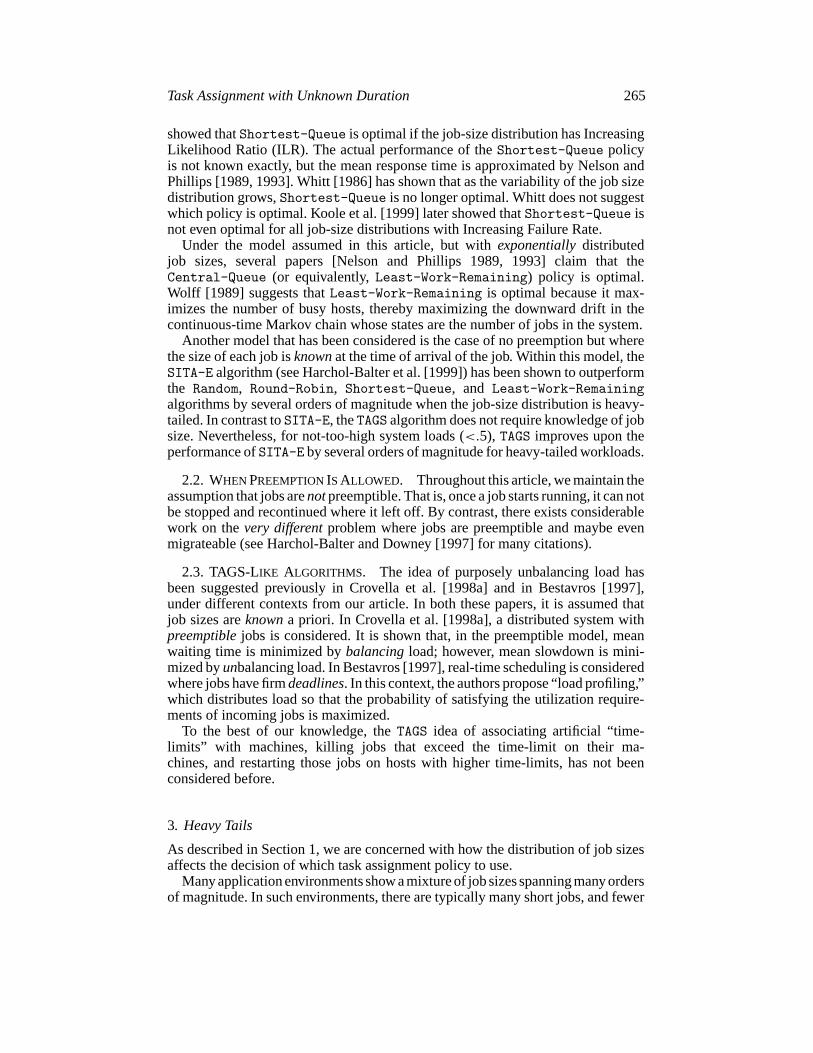
FIG. 3. Measured distribution of UNIX process CPU lifetimes, taken from Harchol-Balter andDowney [1997]. Data indicates fraction of jobs whose CPU service requirement exceedsT seconds,as a function ofT .
long jobs. Much previous work has used theexponentialdistribution to capturethis variability, as described in Section 2. However, recent measurements indicatethat for many applications the exponential distribution is a poor model and that aheavy-taileddistribution is more accurate. In general, a heavy-tailed distribution isone for which
Pr{X > x} ∼ x−α,
where 0< α < 2. The simplest heavy-tailed distribution is theParetodistribution,with probability mass function
f (x) = αkαx−α−1, α, k > 0, x ≥ k,
and cumulative distribution function
F(x) = Pr{X ≤ x} = 1−(
k
x
)α.
A set of job sizes following a heavy-tailed distribution has the following properties:
(1) Decreasing failure rate: In particular, the longer a job has run, the longer it isexpected to continue running.
(2) Infinite variance (and ifα ≤ 1, infinite mean).(3) The property that a tiny fraction (<1%) of the very longest jobs comprise over
half of the total load. We refer to this important property throughout the articleas theheavy-tailed property.
The lower the parameterα, the more variable the distribution, and the more pro-nounced is the heavy-tailed property, that is, the smaller the fraction of long jobsthat comprise half the load.
As a concrete example, Figure 3 depicts graphically on a log-log plot the mea-sured distribution of CPU requirements of over a million UNIX processes, taken
Task Assignment with Unknown Duration 267
from Harchol-Balter and Downey [1997]. This distribution closely fits the curve
Pr{Process CPU requirement> T} = 1
T.
In Harchol-Balter and Downey [1997], it is shown that this distribution is presentin a variety of computing environments, including instructional, research, andadministrative environments.
In fact, heavy-tailed distributions appear to fit many recent measurements ofcomputing systems. These include, for example:
—Unix process CPU requirements measured at Bellcore: 1≤ α ≤ 1.25 [Lelandand Ott 1986].
—Unix process CPU requirements, measured at UC Berkeley:α ≈ 1 [Harchol-Balter and Downey 1997].
—Sizes of files transferred through the Web: 1.1≤ α ≤ 1.3 [Crovella and Bestavros1997; Crovella et al. 1998b].
—Sizes of files stored in Unix filesystems: [Irlam 1994].—I/O times: [Peterson and Adams 1996].—Sizes of FTP transfers in the Internet:.9≤ α ≤ 1.1 [Paxson and Floyd 1995].—Pittsburgh Supercomputing Center (PSC) workloads for distributed servers
consisting of Cray C90 and Cray J90 machines [Schroeder and Harchol-Balter 2000].4
In most of these cases, where estimates ofα were made,α tends to be close to 1,which represents very high variability in job-service requirements.
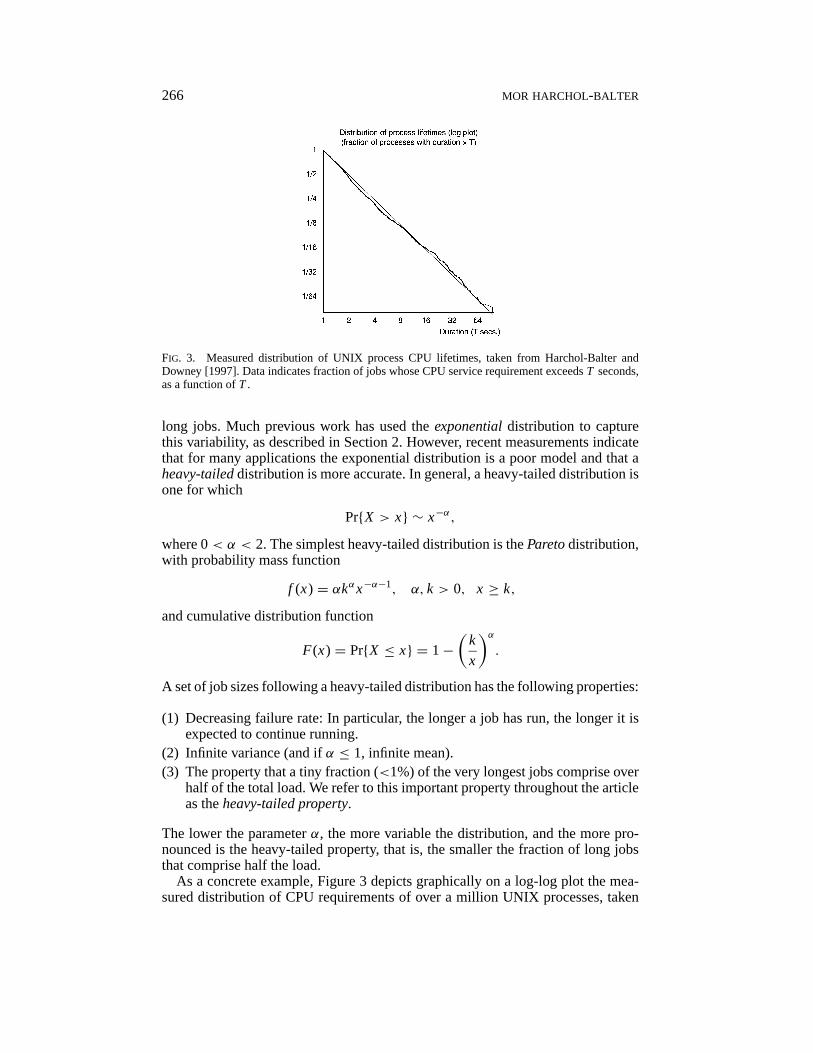
In practice, there is some upper bound on the maximum size of a job, becausefiles only have finite lengths. Throughout this article, we therefore model job sizesas being generated i.i.d. from a distribution that is heavy-tailed, but has an upperbound—a very high one. We refer to this distribution as aBounded Pareto.It ischaracterized by three parameters:α, the exponent of the power law;k, the shortestpossible job; andp, the largest possible job. The probability density function forthe Bounded ParetoB(k, p, α) is defined as:
f (x) = αkα
1− (k/p)αx−α−1 k ≤ x ≤ p. (1)
In this article, we vary theα-parameter over the range 0 to 2 in order to ob-serve the effect ofvariability of the distribution. To focus on the effect of chang-ing variance, we keep the distributional mean fixed (at 3000) and the maximumvalue fixed (atp = 1010), which correspond to typical values taken from Crovellaand Bestavros [1997]. In order to keep the mean constant, we adjustk slightly asα changes (0< k ≤ 1500).
Note that the Bounded Pareto distribution has all its moments finite. Thus, it isnot a heavy-tailed distribution in the sense we have defined above. However, this
4 While the distribution of job processing requirements at the PSC does not seem to exactly fit aPareto distribution, these workloads do have a very strong heavy-tailed property and high variance.Specifically, our measurements showed that half the load is made up by only the biggest 1.3% of alljobs, and the squared coefficient of variation is 43.
268 MOR HARCHOL-BALTER
FIG. 4. Parameters of the Bounded Pareto Distribution (left); Second Moment ofB(k, p = 1010, α)as a function ofα, whenE{X} = 3000 (right).
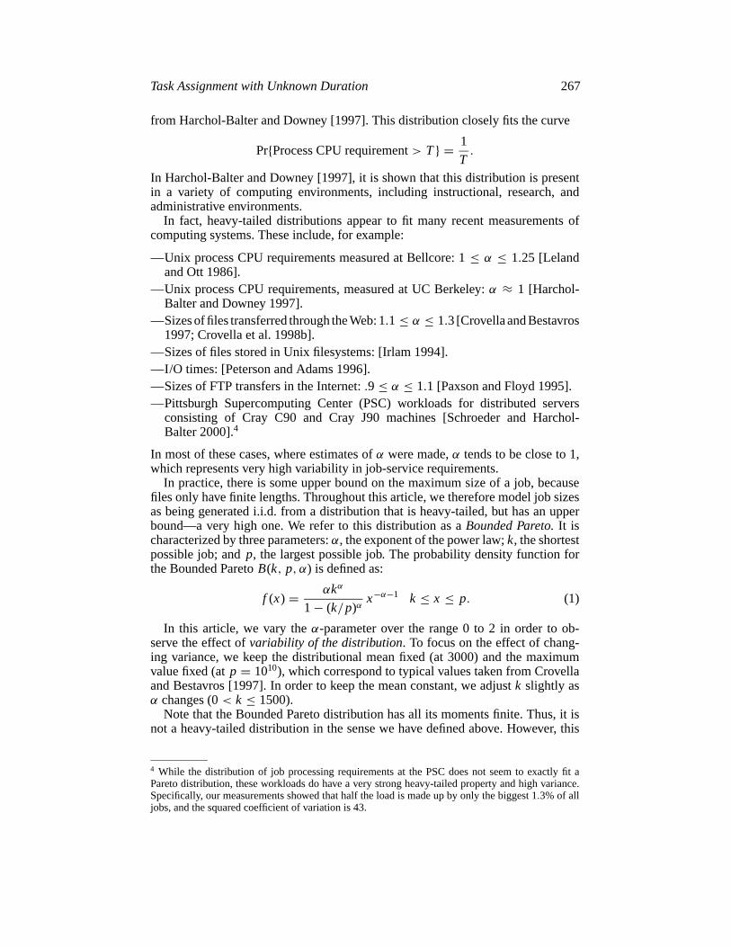
FIG. 5. Illustration of the flow of jobs in theTAGS algorithm.
distribution will still show very high variability ifk ¿ p. For example, Figure 4(right) shows the second momentE{X2} of this distribution as a function ofα forp = 1010, wherek is chosen to keepE{X} constant at 3000, (0< k ≤ 1500).The figure shows that the second moment explodes exponentially asα declines.Furthermore, the Bounded Pareto distribution also still exhibits the heavy-tailedproperty and (to some extent) the decreasing failure rate property of the unboundedPareto distribution. We mention these properties because they are important inchoosing the best task assignment policy.
4. The TAGS Algorithm
This section describes theTAGS algorithm. Leth be the number of hosts in thedistributed server. Think of the hosts as being numbered: 1, 2, . . . , h. Thei th hosthas a numbersi associated with it, wheres1 < s2 < · · · < sh.TAGS works as shown in Figure 5:All incoming jobs are immediately dispatched
to Host 1. There they are serviced in FCFS order. If they complete before usingup s1 amount of CPU, they simply leave the system. However, if a job has useds1 amount of CPU at Host 1 and still has not completed, then it is killed (remember,jobs cannot be preempted). The job is then put at the end of the queue at Host 2,
Task Assignment with Unknown Duration 269
where it must be restarted from scratch.5 Each host services the jobs in its queue inFCFS order. If a job at hosti uses upsi amount of CPU and still has not completedit is killed and put at the end of the queue for Hosti + 1. In this way, theTAGSalgorithm “guesses the size” of each job, hence the name.
TheTAGS algorithm may sound counterintuitive for a few reasons: First of all,there’s a sense that the higher-numbered hosts will be underutilized and the firsthost overcrowded since all incoming jobs are sent to Host 1. An even more vitalconcern is that theTAGS algorithmwastesa large amount of resources by killingjobs and then restarting them from scratch.6 There is also the sense that the big jobsare especially penalized since they are the ones being restarted.TAGS comes in three flavors; these only differ in how thesi ’s are chosen. In
TAGS-opt-slowdown, the si ’s are chosen so as to optimize mean slowdown. InTAGS-opt-waitingtime, thesi ’s are chosen so as to optimize mean waiting time.As we’ll see,TAGS-opt-slowdown andTAGS-opt-waitingtime are not neces-sarily fair. InTAGS-opt-fairness, thesi ’s are chosen so as to optimize fairness.Specifically, the jobs whose final destination is Hosti experience the same expectedslowdown underTAGS-opt-fairness as do the jobs whose final destination isHost j , for all i and j .
To useTAGS, one needs to compute the appropriatesi cutoffs. Thesi ’s are a func-tion of the distribution of job sizes (which in our case is defined by the parametersα,k, andp) and the average outside arrival rateλ. These workload parameters can bedetermined by observing the system for a period of time. To determine thesi ’s, giventhese workload parameters, we useMathematicaTM as described in the Appendix tosolve for the optimal values of thesi ’s, which minimize the performance formulasfor mean slowdown, mean response time, etc.TAGS may seem reminiscent of multilevel feedback queuing, but these arenot
related. In multilevel feedback queuing, there is only a single host with manyvirtualqueues. The host is time-shared and jobs are preemptible. When a job uses someamount of service time, it is transferred (not killed and restarted) to a lower priorityqueue. Also, in multilevel feedback queuing, the jobs in that lower priority queueareonlyallowed to run when the higher priority queues are empty.
5. Analytic Results for the Case of Two Hosts
This section contains the results of our analysis of theTAGS task assignment policyand other policies. In order to clearly explain the effect of theTAGS algorithm, welimit the discussion in this section to the case of two hosts. In this case, we refer tothe jobs whose final destination is Host 1 as theshort jobsand the jobs whose finaldestination is Host 2 as thebig jobs. Until Section 5.3, we always assume that thesystem load is 0.5 and there are two hosts. In Section 5.3, we consider other systemloads, but still stick to the case of two hosts. Finally, in Section 6, we considerdistributed servers with>2 hosts.
We evaluate theRandom,Least-Work-Remaining, andTAGSpolicies via analy-sis, all as a function ofα, whereα is the variance parameter for the Bounded Pareto
5 Note, although the job is restarted, it is still the same job, of course. We must therefore be carefulin our analysisnot to assign it a new service requirement.6 My dad, Micha Harchol, would add that there’s also the psychological concern of what the angryuser might do when he’s told his job has been killed to help the general good.
270 MOR HARCHOL-BALTER
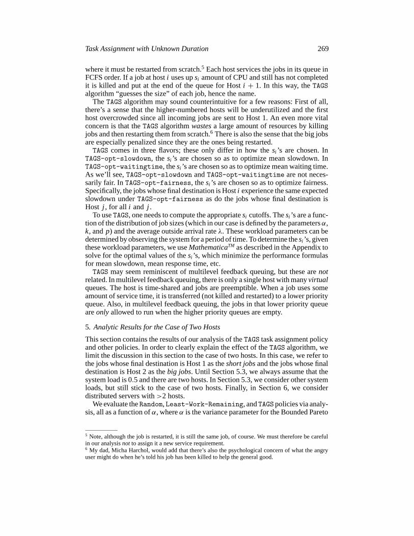
FIG. 6. Mean slowdown for distributed server with two hosts and system load .5 under (a)TAGS-opt-slowdown and (b)TAGS-opt-fairness as compared with theLeast-Work-Remaining andRandom task assignment policies.
job size distribution, andα ranges between 0 and 2. Recall from Section 3 thatthe lowerα is, the higher the variance in the job-size distribution. Recall also thatempirical measurements of job-size distributions often showα ≈ 1.Round-Robin(see Section 1) will not be evaluated directly because we showed in a previouspaper [Harchol-Balter et al. 1999] thatRandom andRound-Robin have almostidentical performance.
Figure 6(a) shows mean slowdown underTAGS-opt-slowdown as com-pared with the other policies. The y-axis is shown on a log scale. Observethat for very highα, the performance of all the task assignment policies is
Task Assignment with Unknown Duration 271
comparable and very good, however asα decreases, the performance of all thepolicies degrades. TheLeast-Work-Remaining policy consistently outper-forms Random by about an order of magnitude; however,TAGS-opt-slowdownoffers several orders of magnitude further improvement: Atα = 1.5, TAGS-opt-slowdown outperformsLeast-Work-Remaining by 2 orders of magnitude;at α≈ 1, TAGS-opt-slowdown outperformsLeast-Work-Remaining by over4 orders of magnitude; atα = .4, TAGS-opt-slowdown outperformsLeast-Work-Remaining by over 9 orders of magnitude.
Figure 6(b) shows mean slowdown ofTAGS-opt-fairness, as compared withthe other policies. Surprisingly, the performance ofTAGS-opt-fairness is not farfrom that ofTAGS-opt-slowdownand yetTAGS-opt-fairnesshas the additionalbenefit of fairness.
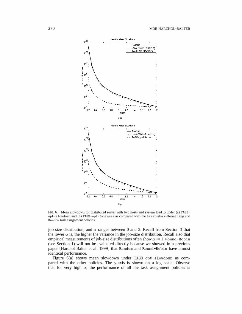
Figure 7 is identical to Figure 6 except that in this case the performance metric ismean waiting time, rather than mean slowdown. Again theTAGS algorithm showsseveral orders of magnitude improvement over the other task assignment policies.
Why does theTAGS algorithm work so well? Intuitively, it seems thatLeast-Work-Remaining should be the best performer, sinceLeast-Work-Remaining sends each job to where it will individually experience the lowest wait-ing time. The reason whyTAGSworks so well is two-fold: The first reason isvariancereduction(Section 5.1) and the second reason isload unbalancing(Section 5.2).
5.1. VARIANCE REDUCTION. Variance reduction refers to reducing the varianceof job sizes that share the same queue. Intuitively, variance reduction improvesperformance because it reduces the chance of a short job getting stuck behind along job in the same queue. This is stated more formally in Theorem 1 below, whichis derived from the Pollaczek–Khinchin formula.
THEOREM 1. Given an M/G/1 FCFS queue, where the arrival process hasrateλ, X denotes the service time distribution, andρ denotes the utilization(ρ =λE{X}). Let W be a job’s waiting time in queue, S be its slowdown, and Q be thequeue length on its arrival. Then,
E{W} = λE{X2}2(1− ρ)
(Pollaczek–Khinchin formula[Pollaczek 1930; Khinchi 1932])
E{S} = E{
W
X
}= E{W} · E{X−1}
E{Q} = λE{W}.PROOF. The slowdown formula follows from the fact thatW andX are inde-
pendent for a FCFS queue, and the queue size follows from Little’s formula.
The above formulas apply to just a single FCFS queue,not a distributed server.Observe that every metric for the simple FCFS queue is dependent onE{X2}, thesecond moment of the service time. Recall that if the workload is heavy-tailed, thesecond moment of the service time explodes (Figure 4). We now discuss the effectof high variability in job sizes on adistributed serverwith h hosts under the varioustask assignment policies.
5.1.1. Random Task Assignment.This policy simply performs Bernoulli split-ting on the input stream, with the result that each host becomes an independent
272 MOR HARCHOL-BALTER
FIG. 7. Mean waiting time for distributed server with two hosts and system load .5 under (a)TAGS-opt-slowdown and (b)TAGS-opt-fairness as compared with theLeast-Work-Remaining andRandom task assignment policies.
M/B(k, p, α)/1 queue. The load at thei th host,ρi , is equal to the system load,ρ. The arrival rate at thei th host is 1/h-fraction of the total outside arrival rate.Theorem 1 applies directly, and all performance metrics are proportional to thesecond moment ofB(k, p, α). Performance is generally poor because the secondmoment of theB(k, p, α) is high.
5.1.2. Round Robin. This policy splits the incoming stream so each host seesan Eh/B(k, p, α)/1 queue, with utilizationρi = ρ, whereEhdenotes anh-stage
Task Assignment with Unknown Duration 273
Erlang distribution. This system has performance close to theRandom policy sinceit still sees high variability in service times, which dominates performance.
5.1.3. Least-Work-Remaining.This policy is equivalent toCentral-Queue,which is simply an M/G/h queue, for which there exist known approximations,[Sozaki and Ross 1978; Wolff 1989]:
E{QM/G/h} = E{QM/G/h} · E{X2}
E{X}2 ,
where X denotes the service time distribution, andQ denotes queue length.What’s important to observe here is that the mean queue length, and thereforethe mean waiting time and mean slowdown, are all proportional to the sec-ond moment of the service time distribution, as was the case for theRandomand Round-Robin policies. In fact, the performance metrics are all propor-tional to the squared coefficient of variation (C2 = E{X2}/E{X}2) of the servicetime distribution.
5.1.4. TAGS. TheTAGS policy is the only policy thatreducesthe variance ofjob sizes at the individual hosts. Consider the jobs that queue at Hosti : First, thereare those jobs are destined for Hosti . Their job-size distribution isB(si−1, si , α)because the original job-size distribution is a Bounded Pareto. Then there are thejobs that are destined for hosts numbered greater thani . The service time of thesejobs at Hosti is capped atsi . Thus, the second moment of the job-size distributionat Hosti is lower than the second moment of the originalB(k, p, α) distribution(for all hosts except the highest numbered host, it turns out). The full analysis oftheTAGS policy is presented in the Appendix. A sketch is given here: The initialdifficulty is figuring out what to condition on, since jobs may visit multiple hosts.The solution is to partition thejobs based on theirfinal host destination. Thus,the mean response time of the system is a linear combination of the mean responsetime of jobs whose final destination is Hosti , where i = 1, . . . , h. The meanresponse time for a job whose final destination is Hosti is the sum of the job’sresponse times at Hosts 1 throughi . The mean response timeat Hosti is computedvia the M/G/1 formula. These computations are relatively straightforward exceptfor one point that we have to approximate and that we explain now: For analyticconvenience, we need to be able to assume that the jobs arriving at each host form aPoisson Process. This is, of course, true for Host 1. However, the arrivals at Hostiare those departures from Hosti − 1 that exceed sizesi−1. They form alessburstyprocess than a Poisson Process since they are spaced apart by at leastsi−1. Sincewe make the assumption that the arrival process into Hosti is a Poisson Process(that is more bursty than the actual process), our analysis if anything produces anupper bound on the response time and slowdown ofTAGS. Finally, once the finalexpression for mean response time is derived,MathematicaTM is used to derivethose cutoffs that minimize the expression.
5.2. LOAD UNBALANCING. The second reason whyTAGS performs so well hasto do withload unbalancing. Observe that all the other task assignment policies wedescribed specifically try tobalanceload at the hosts.Random andRound-Robinbalance the expected load at the hosts, whileLeast-Work-Remaining goes evenfurther in trying to balance the instantaneous load at the hosts. InTAGS, we dothe opposite.
274 MOR HARCHOL-BALTER
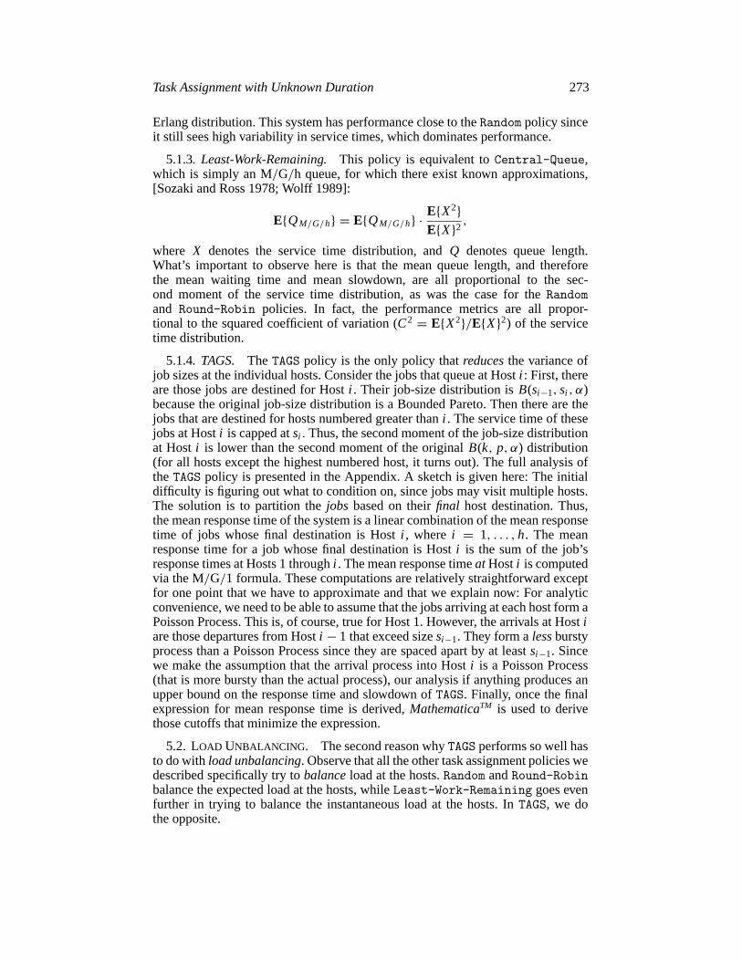
FIG. 8. Load at Host 1 as compared with Host 2 in a distributed server with two hosts and systemload .5 under (a)TAGS-opt-slowdown, (b)TAGS-opt-waitingtime, and (c)TAGS-opt-fairness.Observe that for very lowα, Host 1 is run at load close to zero, and Host 2 is run at load close to 1,whereas for highα, Host 1 is somewhat overloaded.
Figure 8 shows the load at Host 1 and at Host 2 forTAGS-opt-slowdown,TAGS-opt-waitingtime, andTAGS-opt-fairness as a function ofα. Observethat all three flavors ofTAGS (purposely) severely underload Host 1 whenα is lowbut for higherα actually overload Host 1 somewhat. In the middle range,α ≈ 1,the load is balanced in the two hosts.
We first explain why load unbalancing is desirable when optimizing overall meanslowdown of the system. We later explain what happens when optimizing fairness.To understand why it is desirable to operate at unbalanced loads, we need to go backto the heavy-tailed property. The heavy-tailed property says that when a distributionis very heavy-tailed (very lowα), only a miniscule fraction of all jobs—the verylongest ones—are needed to make up more than half the total load. As an example,for the caseα = .2, it turns out that the longest 10−6 fraction of jobs alone areneeded to make up half the load. In fact not many more jobs—just the longest10−4 fraction of all jobs—are needed to make up.99999 fraction of the load. This
Task Assignment with Unknown Duration 275
suggests a load game that can be played: We choose the cutoff point (s1) such thatmostjobs ((1−10−4) fraction) have Host 1 as their final destination, and only a veryfewjobs (the longest 10−4 fraction of all jobs) have Host 2 as their final destination.Because of the heavy-tailed property, the load at Host 2 will be extremely high(.99999) while the load at Host 1 will be very low (.00001). Sincemostjobs get torun at such reduced load, the overall mean slowdown is very low.
When the distribution is a little less heavy-tailed, for example,α ≈ 1, we can’tplay this load unbalancing game as well. Again, we would like to severely underloadHost 1 and overload Host 2. Before, we were able to do this by sending only avery small fraction of all jobs (<10−4 fraction) to Host 2. However, now that thedistribution is not as heavy-tailed, a larger fraction of jobs must have Host 2 as itsfinal destination to create high load at Host 2. But this, in turn, means that jobswith destination Host 2 count more in determining the overall mean slowdownof the system, which is bad since jobs with destination Host 2 experience largerslowdowns. Thus, we can only afford to go so far in overloading Host 2 before itturns against us.
When we get toα > 1, it turns out that it actually pays tooverloadHost 1 a little.This seems counterintuitive, since Host 1 counts more in determining the overallmean slowdown of the system because most jobs have destination Host 1. However,the point is that now it is impossible to create the wonderful state where almost alljobs are on Host 1 and yet Host 1 is underloaded. The tail is just not heavy enough.No matter how we choose the cutoff, a significant portion of the jobs will haveHost 2 as their destination. Thus, Host 2 will inevitably figure into the overall meanslowdown and so we need to keep the performance on Host 2 in check. To do this,it turns out we need to slightly underload Host 2, to make up for the fact that thejob-size variability is so much greater on Host 2 than on Host 1.
The above has been an explanation for why load unbalancing is important withrespect to optimizing the system mean slowdown. However, it is not at all clearwhy load unbalancing also optimizes fairness, as shown in Figure 8(c). UnderTAGS-opt-fairness, the mean slowdown experienced by the short jobs isequalto the mean slowdown experienced by the long jobs. However, it seems in fact thatwe are treating the long jobs unfairly on three counts:
(1) The short jobs run on Host 1 which has very low load (for lowα).(2) The short jobs run on Host 1 which has very lowE{X2}.(3) The short jobs don’t have to be restarted from scratch and wait on a second
line.
So how can it possibly be fair to help the short jobs so much? The answer issimply that the short jobs are short. Thus, they need low waiting times to keeptheir slowdown low. Long jobs, on the other hand, can afford a lot more waitingtime. They are better able to amortize the punishment over their long lifetimes. Itis important to mention, though, that this would not be the case for all distribu-tions. It is because our job-size distribution for lowα is so heavy-tailed that thelong jobs are trulyelephants(way longer than the shorts) and thus can afford tosuffer more.
5.3. DIFFERENT LOADS. Until now, we have studied only the model of adistributed server with two hosts and system load 0.5. In this section we con-sider the effect of system load on the performance ofTAGS. We continue to
276 MOR HARCHOL-BALTER
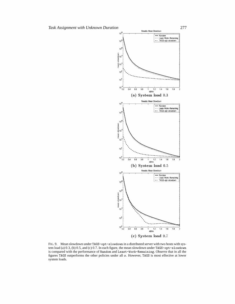
assume a two-host model. Figure 9 shows the performance ofTAGS-opt-slowdownon a distributed server run at system load (a) 0.3, (b) 0.5, and (c) 0.7.In all three figures,TAGS-opt-slowdown improves upon the performance ofLeast-Work-Remaining andRandom under the full range ofα; however, the im-provement ofTAGS-opt-slowdown is much better when the system is more lightlyloaded. In fact, all the policies improve as the system load is dropped; however, theimprovement inTAGS is the most dramatic. In the case where the system load is0.3,TAGS-opt-slowdown improves uponLeast-Work-Remaining by over 4 or-ders of magnitude atα= 1, by 7 orders of magnitude whenα= .6 and by almost20 orders of magnitude whenα= .2! When the system load is 0.7, on the otherhand, TAGS-opt-slowdown behaves comparably toLeast-Work-Remainingfor most α and only improves uponLeast-Work-Remaining in the narrowerrange of .6<α<1.5. Notice however that, atα ≈ 1, the improvement ofTAGS-opt-slowdown is still about 4 orders of magnitude.
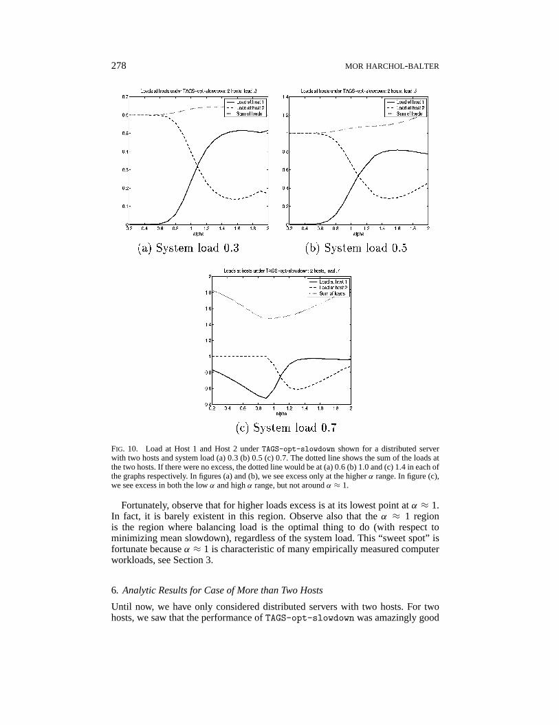
Why is the performance ofTAGS so correlated with load? There are two reasons,both of which are explained by Figure 10, which shows the loads at the two hostsunderTAGS-opt-slowdown in the case where the system load is (a) 0.3, (b) 0.5,and (c) 0.7.
The first reason for the ineffectiveness ofTAGS under high loads is that thehigher the load, the less ableTAGS is to play the load-unbalancing game describedin Section 5.2. For lowerα, TAGS reaps much of its benefit at the lowerα by movingall the load onto Host 2. When the system load is only 0.5, TAGS is easily able topile all the load on Host 2 without exceeding load 1 at Host 2. However, when thesystem load is 0.7, the restriction that the load at Host 2 must not exceed 1 impliesthat Host 1 cannot be as underloaded asTAGSwould like. This is seen by comparingFigure 10(b) and Figure 10(c) where in (c) the load on Host 1 is much higher forthe lowerα than it is in (b).
The second reason for the ineffectiveness ofTAGS under high loads is due towhat we callexcess. Excess is the extra work created inTAGS by restarting jobsfrom scratch. In the two-host case, the excess is simply equal toλ · p2 · s1, whereλ is the outside arrival rate,p2 is the fraction of jobs whose final destination isHost 2, ands1 is the cutoff differentiating short jobs from long jobs. An equivalentdefinition of excess is the difference between the actual sum of the loads on thehosts andh times the system load, whereh is the number of hosts. The dotted linein Figures 10(a)–(c) shows the sum of the loads on the hosts.
Observe that for loads under 0.5, excess is not an issue. The reason is that for lowα, where we need to do the severe load unbalancing, excess is basically nonexistentfor loads 0.5 and under, sincep2 is so small (due to the heavy-tailed property) andsinces1 could be forced down. For highα, excess is present. However, all the taskassignment policies already do well in the highα region because of the low job sizevariability, so the excess is not much of a handicap.
When system load exceeds 0.7, however, excess is much more of a problem, asis evidenced by the dotted line in Figure 10(c). One reason that the excess is worseis simply that overall excess increases with load because excess is proportionalto λ, which is in turn proportional to load. The other reason that the excess isworse at higher loads has to do withs1. In the lowα range, althoughp2 is stilllow (due to the heavy-tailed property),s1 cannot be forced low because the load atHost 2 is capped at 1. Thus, the excess for lowα is very high. In the highα range,excess again is high becausep2 is high.
Task Assignment with Unknown Duration 277
FIG. 9. Mean slowdown underTAGS-opt-slowdown in a distributed server with two hosts with sys-tem load (a) 0.3, (b) 0.5, and (c) 0.7. In each figure, the mean slowdown underTAGS-opt-slowdownis compared with the performance ofRandom andLeast-Work-Remaining. Observe that in all thefiguresTAGS outperforms the other policies under allα. However,TAGS is most effective at lowersystem loads.
278 MOR HARCHOL-BALTER
FIG. 10. Load at Host 1 and Host 2 underTAGS-opt-slowdown shown for a distributed serverwith two hosts and system load (a) 0.3 (b) 0.5 (c) 0.7. The dotted line shows the sum of the loads atthe two hosts. If there were no excess, the dotted line would be at (a) 0.6 (b) 1.0 and (c) 1.4 in each ofthe graphs respectively. In figures (a) and (b), we see excess only at the higherα range. In figure (c),we see excess in both the lowα and highα range, but not aroundα ≈ 1.
Fortunately, observe that for higher loads excess is at its lowest point atα ≈ 1.In fact, it is barely existent in this region. Observe also that theα ≈ 1 regionis the region where balancing load is the optimal thing to do (with respect tominimizing mean slowdown), regardless of the system load. This “sweet spot” isfortunate becauseα ≈ 1 is characteristic of many empirically measured computerworkloads, see Section 3.
6. Analytic Results for Case of More than Two Hosts
Until now, we have only considered distributed servers with two hosts. For twohosts, we saw that the performance ofTAGS-opt-slowdown was amazingly good
Task Assignment with Unknown Duration 279
FIG. 11. Illustration of the claim that anh host system (h > 2) with system loadρ can always beconfigured to produce performance at least as good as a two-host system with system loadρ (althoughtheh-host system has much higher arrival rate).
if the system load was 0.5 or less, but not nearly as good for system load>0.5. Inthis section, we consider the case of more than two hosts.7
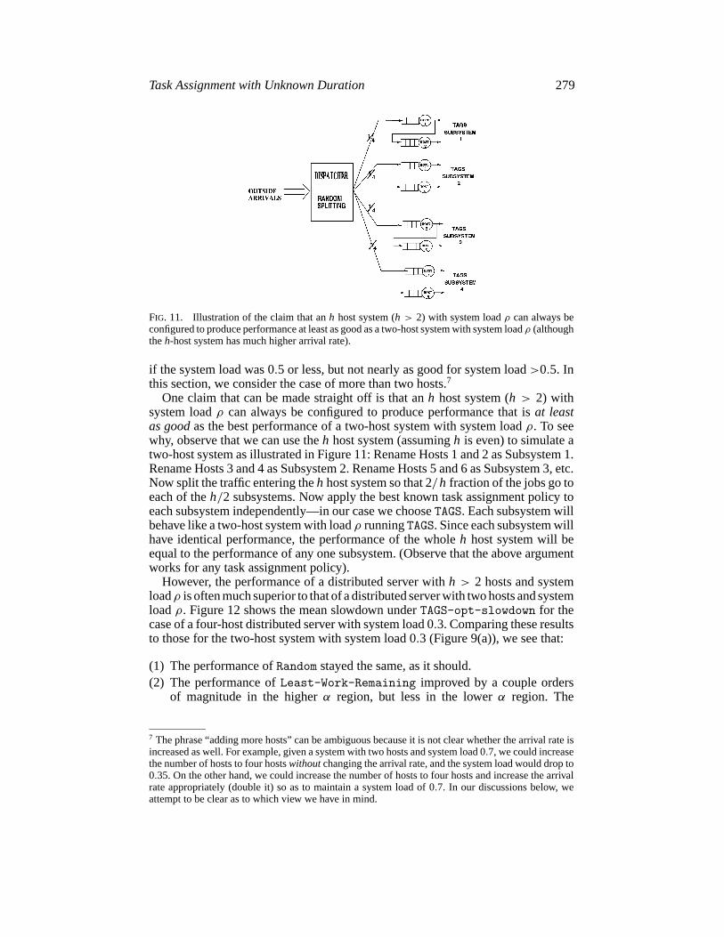
One claim that can be made straight off is that anh host system (h > 2) withsystem loadρ can always be configured to produce performance that isat leastas goodas the best performance of a two-host system with system loadρ. To seewhy, observe that we can use theh host system (assumingh is even) to simulate atwo-host system as illustrated in Figure 11: Rename Hosts 1 and 2 as Subsystem 1.Rename Hosts 3 and 4 as Subsystem 2. Rename Hosts 5 and 6 as Subsystem 3, etc.Now split the traffic entering theh host system so that 2/h fraction of the jobs go toeach of theh/2 subsystems. Now apply the best known task assignment policy toeach subsystem independently—in our case we chooseTAGS. Each subsystem willbehave like a two-host system with loadρ runningTAGS. Since each subsystem willhave identical performance, the performance of the wholeh host system will beequal to the performance of any one subsystem. (Observe that the above argumentworks for any task assignment policy).
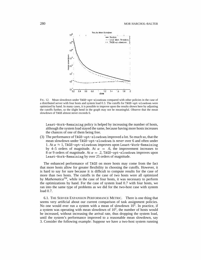
However, the performance of a distributed server withh > 2 hosts and systemloadρ is often much superior to that of a distributed server with two hosts and systemloadρ. Figure 12 shows the mean slowdown underTAGS-opt-slowdown for thecase of a four-host distributed server with system load 0.3. Comparing these resultsto those for the two-host system with system load 0.3 (Figure 9(a)), we see that:
(1) The performance ofRandom stayed the same, as it should.(2) The performance ofLeast-Work-Remaining improved by a couple orders
of magnitude in the higherα region, but less in the lowerα region. The
7 The phrase “adding more hosts” can be ambiguous because it is not clear whether the arrival rate isincreased as well. For example, given a system with two hosts and system load 0.7, we could increasethe number of hosts to four hostswithoutchanging the arrival rate, and the system load would drop to0.35. On the other hand, we could increase the number of hosts to four hosts and increase the arrivalrate appropriately (double it) so as to maintain a system load of 0.7. In our discussions below, weattempt to be clear as to which view we have in mind.
280 MOR HARCHOL-BALTER
FIG. 12. Mean slowdown underTAGS-opt-slowdown compared with other policies in the case ofa distributed server with four hosts and system load 0.3. The cutoffs forTAGS-opt-slowdown wereoptimized by hand. In many cases, it is possible to improve upon the results shown here by adjustingthe cutoffs further, so the slight bend in the graph may not be meaningful. Observe that the meanslowdown ofTAGS almost never exceeds 6.
Least-Work-Remaining policy is helped by increasing the number of hosts,although the system load stayed the same, because having more hosts increasesthe chances of one of them being free.
(3) The performance ofTAGS-opt-slowdown improved a lot. So much so, that themean slowdown underTAGS-opt-slowdown is neverover 6 and often under1. At α ≈ 1, TAGS-opt-slowdown improves uponLeast-Work-Remainingby 4–5 orders of magnitude. Atα = .6, the improvement increases to8 or 9 orders of magnitude. Atα = .2, TAGS-opt-slowdown improves uponLeast-Work-Remaining by over 25 orders of magnitude.
The enhanced performance ofTAGS on more hosts may come from the factthat more hosts allow for greater flexibility in choosing the cutoffs. However, itis hard to say for sure because it is difficult to compute results for the case ofmore than two hosts. The cutoffs in the case of two hosts were all optimizedby MathematicaTM, while in the case of four hosts, it was necessary to performthe optimizations by hand. For the case of system load 0.7 with four hosts, weran into the same type of problems as we did for the two-host case with systemload 0.7.
6.1. THE SERVEREXPANSION PERFORMANCEMETRIC. There is one thing thatseems very artificial about our current comparison of task assignment policies.No one would ever run a system with a mean of slowdown 105. In practice, ifa system was operating with mean slowdown of 105, the number of hosts wouldbe increased, without increasing the arrival rate, thus dropping the system load,until the system’s performance improved to a reasonable mean slowdown, say3. Consider the following example: Suppose we have a two-host system running
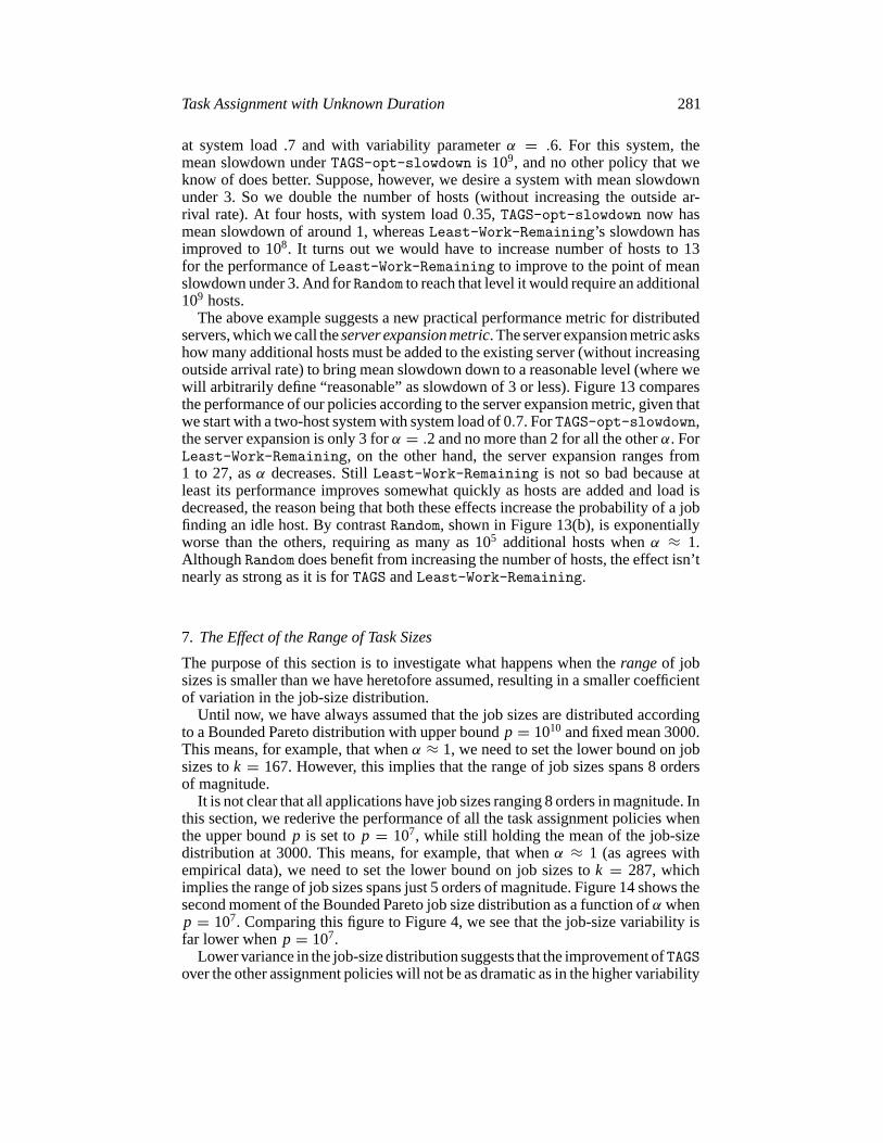
Task Assignment with Unknown Duration 281
at system load .7 and with variability parameterα = .6. For this system, themean slowdown underTAGS-opt-slowdown is 109, and no other policy that weknow of does better. Suppose, however, we desire a system with mean slowdownunder 3. So we double the number of hosts (without increasing the outside ar-rival rate). At four hosts, with system load 0.35, TAGS-opt-slowdown now hasmean slowdown of around 1, whereasLeast-Work-Remaining’s slowdown hasimproved to 108. It turns out we would have to increase number of hosts to 13for the performance ofLeast-Work-Remaining to improve to the point of meanslowdown under 3. And forRandom to reach that level it would require an additional109 hosts.
The above example suggests a new practical performance metric for distributedservers, which we call theserver expansion metric. The server expansion metric askshow many additional hosts must be added to the existing server (without increasingoutside arrival rate) to bring mean slowdown down to a reasonable level (where wewill arbitrarily define “reasonable” as slowdown of 3 or less). Figure 13 comparesthe performance of our policies according to the server expansion metric, given thatwe start with a two-host system with system load of 0.7. ForTAGS-opt-slowdown,the server expansion is only 3 forα = .2 and no more than 2 for all the otherα. ForLeast-Work-Remaining, on the other hand, the server expansion ranges from1 to 27, asα decreases. StillLeast-Work-Remaining is not so bad because atleast its performance improves somewhat quickly as hosts are added and load isdecreased, the reason being that both these effects increase the probability of a jobfinding an idle host. By contrastRandom, shown in Figure 13(b), is exponentiallyworse than the others, requiring as many as 105 additional hosts whenα ≈ 1.AlthoughRandom does benefit from increasing the number of hosts, the effect isn’tnearly as strong as it is forTAGS andLeast-Work-Remaining.
7. The Effect of the Range of Task Sizes
The purpose of this section is to investigate what happens when therangeof jobsizes is smaller than we have heretofore assumed, resulting in a smaller coefficientof variation in the job-size distribution.
Until now, we have always assumed that the job sizes are distributed accordingto a Bounded Pareto distribution with upper boundp = 1010 and fixed mean 3000.This means, for example, that whenα ≈ 1, we need to set the lower bound on jobsizes tok = 167. However, this implies that the range of job sizes spans 8 ordersof magnitude.
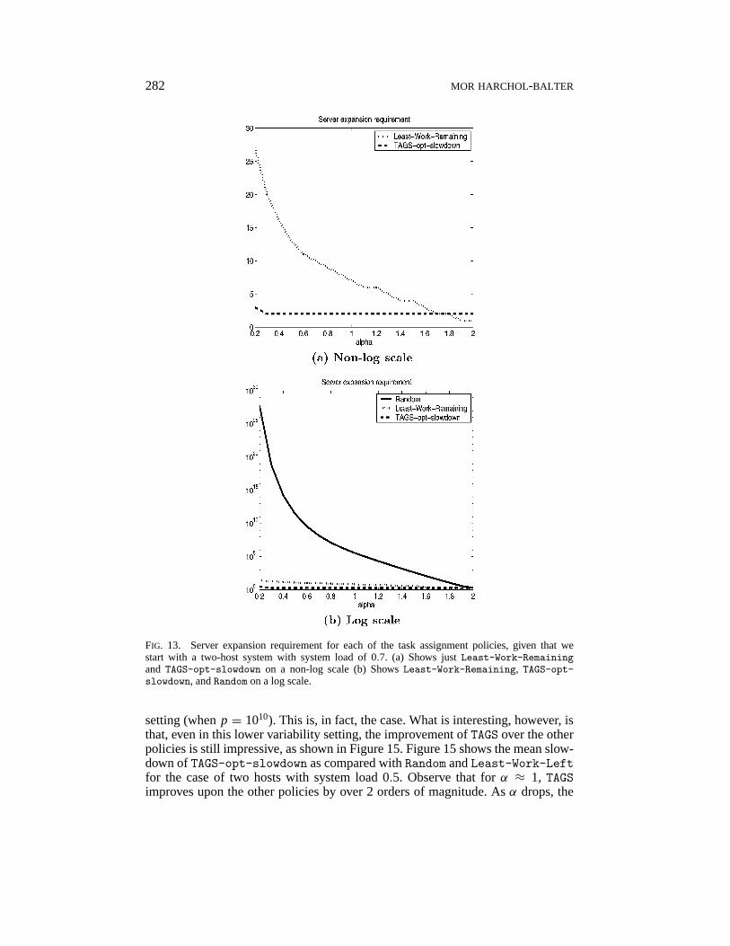
It is not clear that all applications have job sizes ranging 8 orders in magnitude. Inthis section, we rederive the performance of all the task assignment policies whenthe upper boundp is set top = 107, while still holding the mean of the job-sizedistribution at 3000. This means, for example, that whenα ≈ 1 (as agrees withempirical data), we need to set the lower bound on job sizes tok = 287, whichimplies the range of job sizes spans just 5 orders of magnitude. Figure 14 shows thesecond moment of the Bounded Pareto job size distribution as a function ofα whenp = 107. Comparing this figure to Figure 4, we see that the job-size variability isfar lower whenp = 107.
Lower variance in the job-size distribution suggests that the improvement ofTAGSover the other assignment policies will not be as dramatic as in the higher variability
282 MOR HARCHOL-BALTER
FIG. 13. Server expansion requirement for each of the task assignment policies, given that westart with a two-host system with system load of 0.7. (a) Shows justLeast-Work-Remainingand TAGS-opt-slowdown on a non-log scale (b) ShowsLeast-Work-Remaining, TAGS-opt-slowdown, andRandom on a log scale.
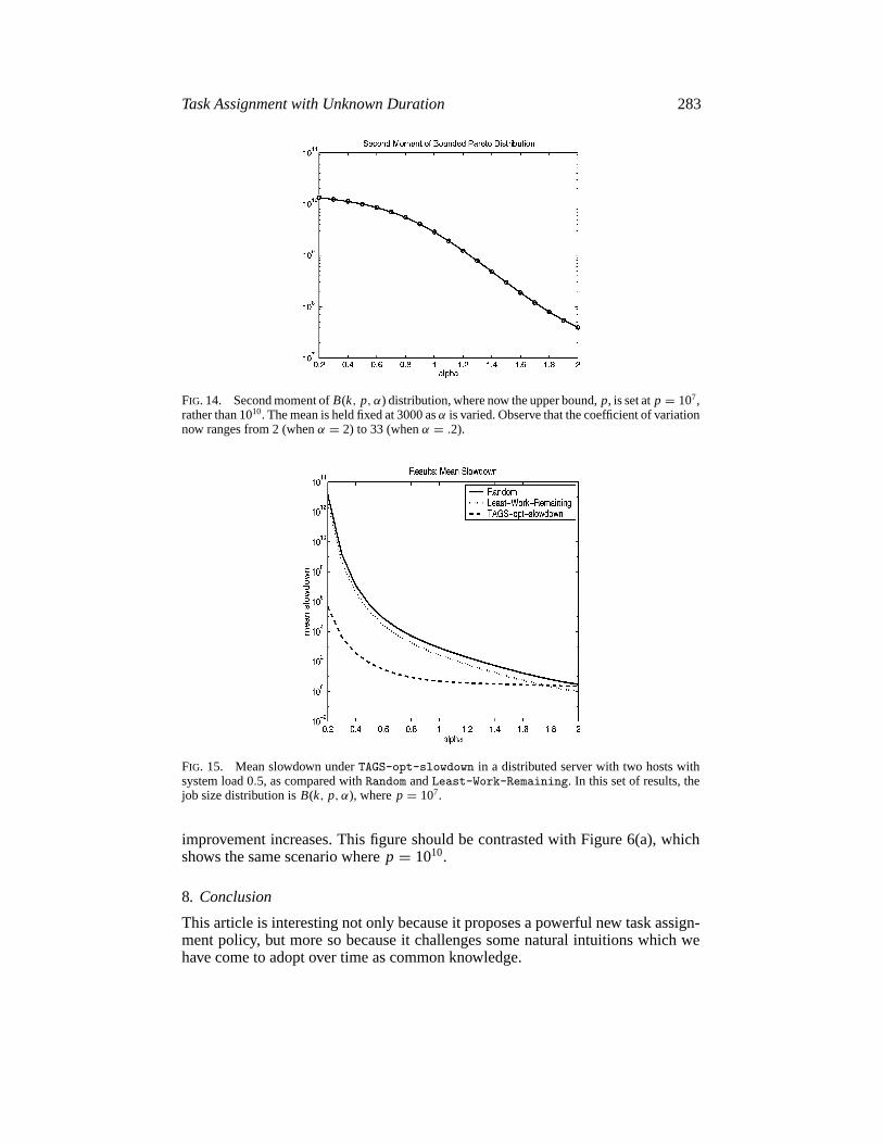
setting (whenp = 1010). This is, in fact, the case. What is interesting, however, isthat, even in this lower variability setting, the improvement ofTAGS over the otherpolicies is still impressive, as shown in Figure 15. Figure 15 shows the mean slow-down ofTAGS-opt-slowdown as compared withRandom andLeast-Work-Leftfor the case of two hosts with system load 0.5. Observe that forα ≈ 1, TAGSimproves upon the other policies by over 2 orders of magnitude. Asα drops, the
Task Assignment with Unknown Duration 283
FIG. 14. Second moment ofB(k, p, α) distribution, where now the upper bound,p, is set atp = 107,rather than 1010. The mean is held fixed at 3000 asα is varied. Observe that the coefficient of variationnow ranges from 2 (whenα = 2) to 33 (whenα = .2).
FIG. 15. Mean slowdown underTAGS-opt-slowdown in a distributed server with two hosts withsystem load 0.5, as compared withRandom andLeast-Work-Remaining. In this set of results, thejob size distribution isB(k, p, α), wherep = 107.
improvement increases. This figure should be contrasted with Figure 6(a), whichshows the same scenario wherep = 1010.
8. Conclusion
This article is interesting not only because it proposes a powerful new task assign-ment policy, but more so because it challenges some natural intuitions which wehave come to adopt over time as common knowledge.
284 MOR HARCHOL-BALTER
Traditionally, the area of task assignment, load balancing and load sharing hasconsisted of heuristics that seek to balance the load among the multiple hosts.TAGS, on the other hand, specifically seeks to unbalance the load, and sometimesseverely unbalance the load. Traditionally, the idea of killing a job and restart-ing it from scratch on a different machine is viewed with skepticism, but possi-bly tolerable if the new host is idle.TAGS, on the other hand, kills jobs and thenrestarts them from scratch at a target host which is typically operating at extremelyhigh load, much higher load than the original source host. Furthermore,TAGS pro-poses restarting the same job multiple times. Traditionally optimal performanceand fairness are viewed as conflicting goals. InTAGS, fairness and optimality aresurprisingly close.
It is interesting to consider further implications of these results, outside the scopeof task assignment. Consider, for example, the question of scheduling CPU-boundjobs on a single CPU, where jobs are not preemptible and no a priori knowledgeis given about the jobs. At first, it seems that FCFS scheduling is the only op-tion. However, in the face of high job-size variability, FCFS may not be wise.This article suggests that killing and restarting jobs may be worth investigat-ing as an alternative, if the load on the CPU is low enough to tolerate the extrawork created.
This work may also have implications in the area of network flow routing. A veryinteresting recent paper by Shaikh et al. [1999] takes a first step in this direction. Thearticle discusses routing of IP flows (which also have heavy-tailed size distributions)and recommends routing long flows differently from short flows.
Appendix
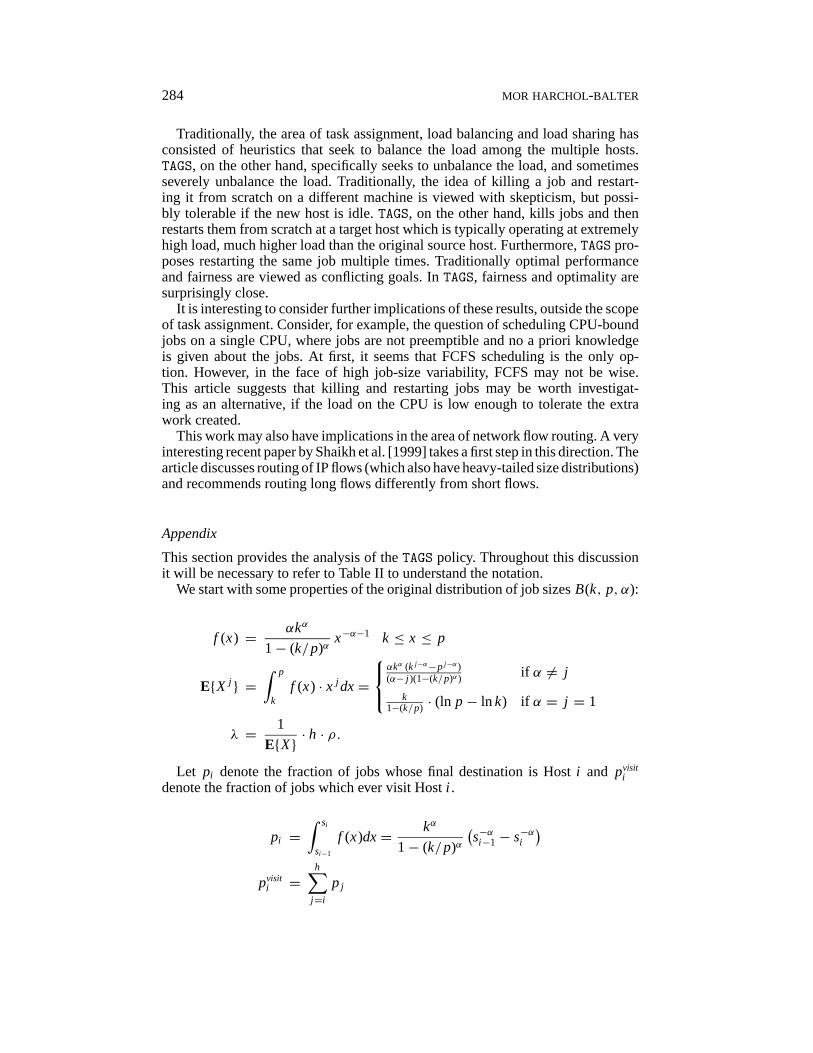
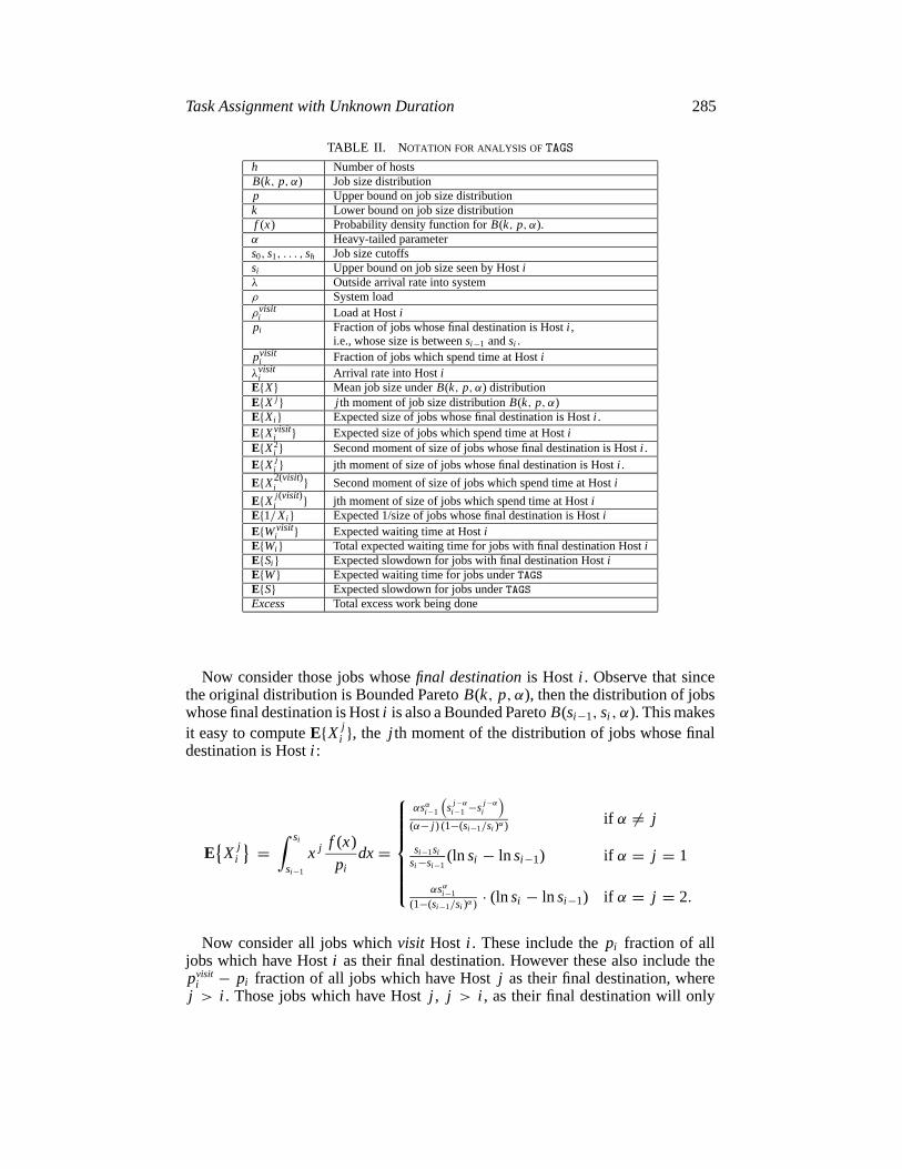
This section provides the analysis of theTAGS policy. Throughout this discussionit will be necessary to refer to Table II to understand the notation.
We start with some properties of the original distribution of job sizesB(k, p, α):
f (x) = αkα
1− (k/p)αx−α−1 k ≤ x ≤ p
E{X j } =∫ p
kf (x) · x j dx=
αkα (k j−α−pj−α)(α− j )(1−(k/p)α) if α 6= j
k1−(k/p) · (ln p− ln k) if α = j = 1
λ = 1
E{X} · h · ρ.
Let pi denote the fraction of jobs whose final destination is Hosti and pvisiti
denote the fraction of jobs which ever visit Hosti .
pi =∫ si
si−1
f (x)dx= kα
1− (k/p)α(s−αi−1− s−αi
)pvisit
i =h∑
j=i
pj
Task Assignment with Unknown Duration 285
TABLE II. NOTATION FOR ANALYSIS OFTAGS
h Number of hostsB(k, p, α) Job size distributionp Upper bound on job size distributionk Lower bound on job size distributionf (x) Probability density function forB(k, p, α).α Heavy-tailed parameters0, s1, . . . , sh Job size cutoffssi Upper bound on job size seen by Hostiλ Outside arrival rate into systemρ System loadρvisit
i Load at Hostipi Fraction of jobs whose final destination is Hosti ,
i.e., whose size is betweensi−1 andsi .pvisit
i Fraction of jobs which spend time at Hostiλvisit
i Arrival rate into HostiE{X} Mean job size underB(k, p, α) distributionE{X j } j th moment of job size distributionB(k, p, α)E{Xi } Expected size of jobs whose final destination is Hosti .E{Xvisit
i } Expected size of jobs which spend time at HostiE{X2
i } Second moment of size of jobs whose final destination is Hosti .E{X j
i } jth moment of size of jobs whose final destination is Hosti .
E{X2(visit)i } Second moment of size of jobs which spend time at Hosti
E{X j (visit)i } jth moment of size of jobs which spend time at Hosti
E{1/Xi } Expected 1/size of jobs whose final destination is HostiE{Wvisit
i } Expected waiting time at HostiE{Wi } Total expected waiting time for jobs with final destination HostiE{Si } Expected slowdown for jobs with final destination HostiE{W} Expected waiting time for jobs underTAGSE{S} Expected slowdown for jobs underTAGSExcess Total excess work being done
Now consider those jobs whosefinal destinationis Host i . Observe that sincethe original distribution is Bounded ParetoB(k, p, α), then the distribution of jobswhose final destination is Hosti is also a Bounded ParetoB(si−1, si , α). This makesit easy to computeE{X j
i }, the j th moment of the distribution of jobs whose finaldestination is Hosti :
E{X j
i
} = ∫ si
si−1
x j f (x)
pidx=
αsαi−1
(sj−αi−1 −sj−α
i
)(α− j ) (1−(si−1/si )α) if α 6= j
si−1si
si−si−1(ln si − ln si−1) if α = j = 1
αsαi−1
(1−(si−1/si )α) · (ln si − ln si−1) if α = j = 2.
Now consider all jobs whichvisit Host i . These include thepi fraction of alljobs which have Hosti as their final destination. However these also include thepvisit
i − pi fraction of all jobs which have Hostj as their final destination, wherej > i . Those jobs which have Hostj , j > i , as their final destination will only
286 MOR HARCHOL-BALTER
have a service requirement ofsi at Hosti . Thus, it follows that:
E{Xvisit
i
} = pi
pvisiti
· E{Xi } + pvisiti − pi
pvisiti
· si
E{X2(visit)
i
} = pi
pvisiti
· E{X2i
}+ pvisiti − pi
pvisiti
· s2i
λvisiti = λ · pvisit
i
ρvisiti = λvisit
i · E{Xvisit
i
}E{1/X j
i
} = E{X− j
i
}There are two equivalent ways of defining excess. We show both below and check
them against each other in our computations.
true-sum-of-loads=h∑
i=1
ρvisiti
desired-sum-of-loads= h · ρExcessa = true-sum-of-loads− desired-sum-of-loads
Excessb =h∑
i=2
λvisiti · si−1
Excess= Excessa = Excessb
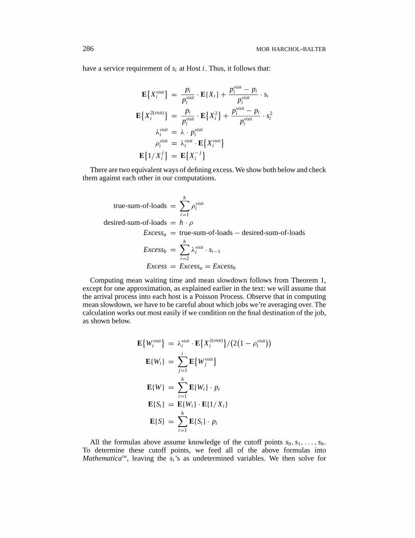
Computing mean waiting time and mean slowdown follows from Theorem 1,except for one approximation, as explained earlier in the text: we will assume thatthe arrival process into each host is a Poisson Process. Observe that in computingmean slowdown, we have to be careful about which jobs we’re averaging over. Thecalculation works out most easily if we condition on the final destination of the job,as shown below.
E{Wvisit
i
} = λvisiti · E
{X2(visit)
i
}/(2(1− ρvisit
i
))E{Wi } =
i∑j=1
E{Wvisit
j
}E{W} =
h∑i=1
E{Wi } · pi
E{Si } = E{Wi } · E{1/Xi }
E{S} =h∑
i=1
E{Si } · pi
All the formulas above assume knowledge of the cutoff pointss0, s1, . . . , sh.To determine these cutoff points, we feed all of the above formulas intoMathematicaTM, leaving thesi ’s as undetermined variables. We then solve for
Task Assignment with Unknown Duration 287
the optimal setting of thesi ’s which minimizes the mean slowdown, mean waitingtime, or fairness, as desired, subject to conditions that the load at each host staysbelow 1.
REFERENCES
BESTAVROS, A. 1997. Load profiling: A methodology for scheduling real-time tasks in a distributedsystem. InProceedings of ICDCS ’97(May).
CROVELLA, M. E.,AND BESTAVROS, A. 1997. Self-similarity in World Wide Web traffic: Evidence andpossible causes.IEEE/ACM Trans. Netw. 5, 6 (Dec.), 835–846.
CROVELLA, M. E., HARCHOL-BALTER, M., AND MURTA, C. 1998a. Task assignment in a distributedsystem: Improving performance by unbalancing load. InProceeding of ACM Sigmetrics Conference onMeasurement and Modeling of Computer Systems Poster Session. ACM, New York.
CROVELLA, M. E., TAQQU, M. S., AND BESTAVROS, A. 1998b. Heavy-tailed probability distributionsin the World Wide Web. InA Practical Guide to Heavy Tails. Chapman & Hall, New York, chap. 1,pp. 1–23.
DOWNEY, A. B. 1997. A parallel workload model and its implications for processor allocation. InProceedings of High Performance Distributed Computing(Aug.). pp. 112–123.
EPHREMIDES, A., VARAIYA , P.,AND WALRAND, J. 1980. A simple dynamic routing problem.IEEE Trans.Automat. Cont. AC-25, 4, 690–693.
FEITELSON, D., AND JETTE, M. A. 1997. Improved utilization and responsiveness with gang scheduling.In Proceedings of IPPS/SPDP ’97 Workshop(Apr.). Lecture Notes in Computer Science, vol. 1291.Springer-Verlag, New York, pp. 238–261.
FEITELSON, D., RUDOLPH, L., SCHWIEGELSHOHN, U., SEVCIK, K., AND WONG, P. 1997. Theory andpractice in parallel job scheduling. InProceedings of IPPS/SPDP ’97 Workshop(Apr.), Lecture Notesin Computer Science, vol. 1291. Springer-Verlag, New York, pp. 1–34.
HARCHOL-BALTER, M., CROVELLA, M., AND MURTA, C. 1999. On choosing a task assignment policyfor a distributed server system.J. Paral. Distr. Comput. 59, 204–228.
HARCHOL-BALTER, M., AND DOWNEY, A. 1997. Exploiting process lifetime distributions for dynamicload balancing.ACM Trans. Comput. Syst. 15, 3.
IRLAM, G. 1994. Unix file size survey—1993. Available athttp://www.base.com/gordoni/ufs93.html.
KHINCHIN, A. Y. 1932. Mathematical theory of stationary queues.Mat. Sbornik 39, 73–84.KOOLE, G., SPARAGGIS, P.,AND TOWSLEY, D. 1999. Minimizing response times and queue lengths in
systems of parallel queues.J. Appl. Prob. 36, 1185–1193.LEISERSON, C. 1998a. The Pleiades alpha cluster at M.I.T. Documentation at: http://bonanza.lcs.
mit.edu.LEISERSON, C. 1998b. The Xolas supercomputing project at M.I.T. Documentation available at:
http://xolas.lcs.mit.edu.LELAND, W. E.,AND OTT, T. J. 1986. Load-balancing heuristics and process behavior. InProceedings
of Performance and ACM SIGMETRICS. ACM, New York, pp. 54–69.NELSON, R. D., AND PHILIPS, T. K. 1989. An approximation to the response time for shortest queue
routing.Perf. Eval. Rev. 7, 1, 181–189.NELSON, R. D., AND PHILIPS, T. K. 1993. An approximation for the mean response time for shortest
queue routing with general interarrival and service times.Perf. Eval. 17, 123–139.PARSONS, E. W., AND SEVCIK, K. C. 1997. Implementing multiprocessor scheduling disciplines. In
Proceedings of IPPS/SPDP ’97 Workshop(Apr.), Lecture Notes in Computer Science, vol. 1459.Springer-Verlag, New York, pp. 166–182.
PAXSON, V., AND FLOYD, S. 1995. Wide-area traffic: The failure of Poisson modeling.IEEE/ACM Trans.Netw.(June), 226–244.
PETERSON, D. L., AND ADAMS, D. R. 1996. Fractal patterns in DASD I/O traffic. InCMG Proc.POLLACZEK, F. 1930. Uber eine aufgabe dev wahrscheinlichkeitstheorie.I-II Math. Zeitschrift. 32,
64–100.THE PSC’S CRAY J90’S. 1998. http://www.psc.edu/machine/cray/j90/j90.html.Supercomputing at the NAS facility. 1998. http://www.nas.nasa.gov/Technology/Supercomputing/.RUDOLPH, L., AND SMITH, P. H. 2000. Valuation of ultra-scale computing systems. InProceedings
of the 6th Workshop on Job Scheduling Strategies for Parallel Processing(Cancun, Mexico, May).
288 MOR HARCHOL-BALTER
Lecture Notes in Computer Science, vol. 1911. Springer-Verlag, New York, http:/www.cs.huji.ac.il/∼feit/parsched/parsched00.html.
SCHROEDER, B., AND HARCHOL-BALTER, M. 2000. Evaluation of task assignment policies for super-computing servers: The case for load unbalancing and fairness. InProceedings of the 9th IEEE Sympo-sium on High Performance Distributed Computing(Aug.) IEEE Computer Society Press, Los Alamitos,Calif.
SHAIKH , A., REXFORD, J., AND SHIN, K. G. 1999. Load-sensitive routing of long-lived ip flows. InProceedings of SIGCOMM(Sept.). ACM, New York.
SOZAKI, S., AND ROSS, R. 1978. Approximations in finite capacity multiserver queues with poissonarrivals.J. Appl. Prob. 13, 826–834.
WHITT, W. 1986. Deciding which queue to join: Some counterexamples.Oper. Res. 34, 1 (Jan.). 226–244.WINSTON, W. 1977. Optimality of the shortest line discipline.J. Appl. Prob. 14, 181–189.WOLFF, R. W. 1989. Stochastic Modeling and the Theory of Queues.Prentice-Hall, Englewood
Cliffs, N.J.
RECEIVED MARCH2000;REVISED JANUARY2001;ACCEPTED JANUARY2002
Journal of the ACM, Vol. 49, No. 2, March 2002.