Embed Size (px)
Citation preview

Specialist Professional and Technical
Services (SPATS) Framework
Lot 1
Task 515 Air Quality Barrier CFD Modelling
March 2019

Air Quality Barrier CFD Modelling Lot 1 SPATS Framework
Specialist Professional and Technical Services (SPaTS) Framework, Lot 1, Task 515
Reference Number: 1-515
Client Name: Highways England
This document has been issued and amended as follows:
Version Date Description Created By Verified By Approved By Rev 1 September
2018 Air Quality Barrier CFD Modelling
Andy Salmon / David Bagshaw
Sam Pollard / Christophe Mabilat
Paul J Taylor
Rev 2 December 2018
Air Quality Barrier CFD Modelling – additional work
Emily Leach David Bagshaw / Sam Pollard
Paul J Taylor
Rev 3 March 2019
Incorporating client comments
David Bagshaw Sam Pollard Paul J Taylor
This report has been prepared for Highways England in accordance with the terms and conditions of appointment stated in the Atkins CH2M SPaTS Agreements. Atkins CH2M JV cannot accept any responsibility for any use of or reliance on the contents of this report by any third party.

Air Quality Barrier CFD Modelling Lot 1 SPATS Framework
Specialist Professional and Technical Services (SPaTS) Framework, Lot 1, Task 515
Table of Contents
1. Introduction ..................................................................................................................................... 1
Background ..................................................................................................................................... 1
Air Quality Barrier Designs .............................................................................................................. 1
2. Aims and Objectives ........................................................................................................................ 1
Objectives ....................................................................................................................................... 1
3. Study Definition ............................................................................................................................... 1
Barrier Design Comparison ............................................................................................................. 1
Barrier Design Optimisation ............................................................................................................. 1
Real World Factors .......................................................................................................................... 2
Additional Wind Conditions .............................................................................................................. 2
4. CFD Modelling ................................................................................................................................ 3
Introduction ..................................................................................................................................... 3
Domain ............................................................................................................................................ 3
Geometry ........................................................................................................................................ 3
Boundary Definition ......................................................................................................................... 4
Wind Profile ..................................................................................................................................... 4
Traffic Modelling .............................................................................................................................. 5
Forces ............................................................................................................................................. 5
Traffic Emissions ............................................................................................................................. 6
Monitoring ....................................................................................................................................... 7
Computational Mesh ....................................................................................................................... 7
Turbulence Model ............................................................................................................................ 8
5. Barrier Performance ........................................................................................................................ 9
No Barrier Case............................................................................................................................. 10
Dordrecht Barrier ........................................................................................................................... 11
Vertical Barrier – 9.3 m .................................................................................................................. 12
Vertical Barrier – 6.0 m .................................................................................................................. 13
6. Barrier Comparison ....................................................................................................................... 15
Monitor Point Transects ................................................................................................................. 15
7. Optimisation .................................................................................................................................. 17
Introduction ................................................................................................................................... 17
Optimisation Procedure ................................................................................................................. 17
Optimisation Methodology ............................................................................................................. 17
Geometry Parameterisation ........................................................................................................... 17
Results .......................................................................................................................................... 18
8. Additional considerations (Real World Effects) .............................................................................. 23
Introduction ................................................................................................................................... 23
Traffic at Standstill ......................................................................................................................... 23
A Building in the Lee of the Barrier ................................................................................................ 25

Air Quality Barrier CFD Modelling Lot 1 SPATS Framework
Specialist Professional and Technical Services (SPaTS) Framework, Lot 1, Task 515
Time-varying Dispersion ................................................................................................................ 27
9. Additional Wind Conditions ............................................................................................................ 29
10. Conclusions & Recommendations ................................................................................................. 41
11. References .................................................................................................................................... 43
Appendix 1 – Figures .............................................................................................................................. 44
Appendix 2 – Sensitivity Test .................................................................................................................. 45

Air Quality Barrier CFD Modelling Lot 1 SPATS Framework
Specialist Professional and Technical Services (SPaTS) Framework, Lot 1, Task 515 1
1. Introduction
Background Exceedances of the annual mean nitrogen dioxide (NO2) Air Quality Strategy (AQS) objective / EU Limit Value adjacent to sections of the Strategic Road Network (SRN) can affect nearby sensitive receptors and be a potential constraint to the delivery of Highway England (HE) schemes. The installation of barriers, which physically influence the dispersion of road traffic emissions between the point of emission and neighbouring sensitive receptors, is potentially a measure available to HE by which annual mean NO2 concentrations can be reduced at receptors in close proximity to the SRN and / or which can be used to mitigate additional adverse air quality impacts associated with proposed HE schemes (i.e. the incremental impact of the proposed scheme).
As part of the Road Investment Strategy, the government established a £100 million Air Quality Designated Fund to improve air quality adjacent to the SRN. The Highways England Air Quality Strategy (HEAQS) sets out the planned approach and activities to achieve this goal, including a commitment to “explore new and innovative approaches to improve air quality” and a reference to trials which are being used to “investigate if barriers can help contribute to improving air quality for our neighbours”. The HEAQS also indicates that the results from the monitoring of such trials will be used to understand if barriers have been successful in improving local air quality and therefore have the potential to be more widely implemented. Highways England also commits to “where appropriate, design out or mitigate poor air quality for our schemes”, which could be another potential application of air quality barriers.
This study is part of a wider programme which seeks to implement barriers at multiple locations adjacent to the SRN, where practical and effective to do so, in order to reduce annual mean NO2 concentrations in problem areas. The outcomes of this study would subsequently inform this wider programme.
Air Quality Barrier Designs Physical barriers in Holland have been shown to reduce pollutants adjacent to the road network (Ref. [1]). Barrier designs may act passively, by deflecting the polluted air upwards, or by containing pollutants close to the carriageway and using the momentum imparted by the traffic flow to draw the pollutant away from sensitive roadside receptors. Active barrier designs operate in a similar way but also contain catalysts to neutralise pollutants that come into contact with it.
Vertical Barrier A vertical barrier is the simplest form of passive barrier geometry and consists of a single straight fence located immediately adjacent to the carriageway. Typically, such barriers found on the SRN are designed to ameliorate traffic noise at properties adjacent to the road network, however they may also have the potential to reduce air pollutant concentrations in their lee. In order to assess their potential, in 2015 Highways England began trialling a 100m long vertical barrier adjacent to the M62 (initially 4 metres high, raised to 6 metres in early 2016). It is understood that the results of this trial were inconclusive however, in terms of the potential effectiveness of such a barrier in reducing NO2 concentrations.
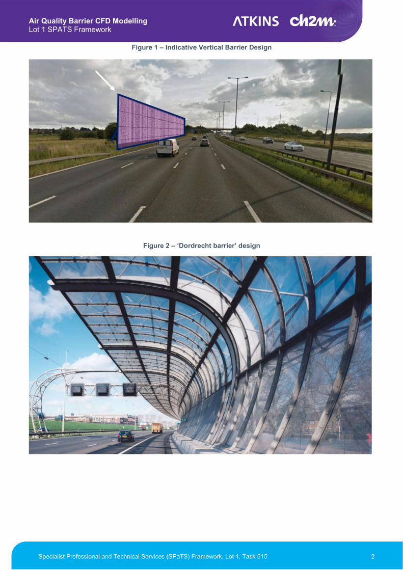
Dordrecht barrier The ‘Dordrecht’ barrier is a passive barrier, its design is more complex than the vertical barrier, with a curved shape and cantilever that overhangs a section of the road. The Dordrecht installation consists of a 1 km length of transparent acrylate formed into a curved surface and built around concrete trusses, reinforced with steel girders. The primary design driver was to lower noise levels and improve air quality (Ref. [2]) at the residential properties close to the A16 motorway near Dordrecht – the extreme vicinity of the housing to the motorway prevented a conventional vertical screen as at least two lanes of the carriageway were required to be covered.
Whilst the design of the Dordrecht barrier appears to be effective in reducing annual mean NO2 concentrations (Ref. [1]), it is understood that this design is costly and therefore the extensive implementation of such barriers alongside the SRN is unlikely to be affordable.
Air Quality Barrier CFD Modelling Lot 1 SPATS Framework
Specialist Professional and Technical Services (SPaTS) Framework, Lot 1, Task 515 2
Figure 1 – Indicative Vertical Barrier Design
Figure 2 – ‘Dordrecht barrier’ design
Air Quality Barrier CFD Modelling Lot 1 SPATS Framework
Specialist Professional and Technical Services (SPaTS) Framework, Lot 1, Task 515 1
2. Aims and Objectives
Whilst previous, monitoring studies undertaken on behalf of Highways England were inconclusive in terms of the potential effectiveness of a vertical, four to six metre high barrier in reducing NO2 concentrations, emerging results from measurements of NO2 undertaken by Highways England around a noise barrier on the A16 near Dordrecht suggest some level of reduction in NO2 concentrations behind this barrier.
The Dordrecht barrier is however of a more complex design than a conventional vertical barrier, with a curved barrier and cantilever that overhangs a section of the road. It is also, at 9.3 m in height, some three metres taller than the tallest vertical barrier trialled previously by Highways England. Whilst the design of the Dordrecht barrier appears to potentially be effective in reducing annual mean NO2 concentrations, it is understood that this design is expensive (relative to a vertical barrier for example), which would potentially limit the number and / or extent of such barriers that could be implemented by Highways England under the Air Quality Designated Fund.
Highways England therefore wish to understand whether a vertical barrier design, taller than that tested by Highways England to date, and / or a simpler, cantilever barrier design, would potentially offer the same level of improvement in annual mean NO2 concentrations as the Dordrecht barrier design, whilst also being easier and more cost-effective to deliver.
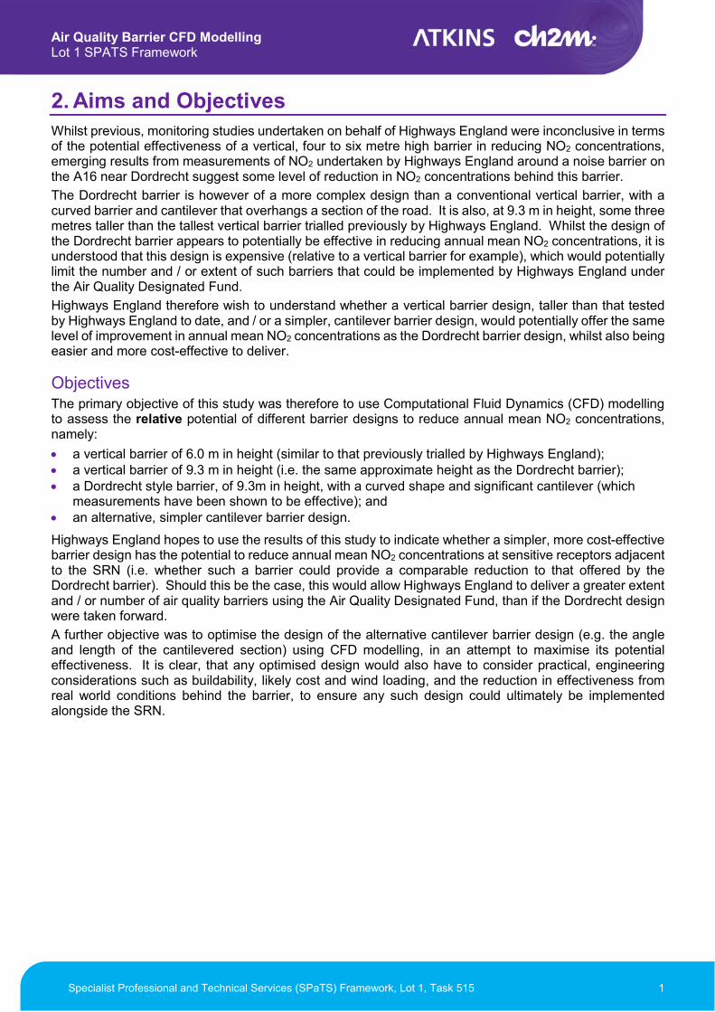
Objectives The primary objective of this study was therefore to use Computational Fluid Dynamics (CFD) modelling to assess the relative potential of different barrier designs to reduce annual mean NO2 concentrations, namely:
a vertical barrier of 6.0 m in height (similar to that previously trialled by Highways England); a vertical barrier of 9.3 m in height (i.e. the same approximate height as the Dordrecht barrier); a Dordrecht style barrier, of 9.3m in height, with a curved shape and significant cantilever (which
measurements have been shown to be effective); and an alternative, simpler cantilever barrier design.
Highways England hopes to use the results of this study to indicate whether a simpler, more cost-effective barrier design has the potential to reduce annual mean NO2 concentrations at sensitive receptors adjacent to the SRN (i.e. whether such a barrier could provide a comparable reduction to that offered by the Dordrecht barrier). Should this be the case, this would allow Highways England to deliver a greater extent and / or number of air quality barriers using the Air Quality Designated Fund, than if the Dordrecht design were taken forward.
A further objective was to optimise the design of the alternative cantilever barrier design (e.g. the angle and length of the cantilevered section) using CFD modelling, in an attempt to maximise its potential effectiveness. It is clear, that any optimised design would also have to consider practical, engineering considerations such as buildability, likely cost and wind loading, and the reduction in effectiveness from real world conditions behind the barrier, to ensure any such design could ultimately be implemented alongside the SRN.
Air Quality Barrier CFD Modelling Lot 1 SPATS Framework
Specialist Professional and Technical Services (SPaTS) Framework, Lot 1, Task 515 1
3. Study Definition
This study is divided into the following subtasks, each of which is defined below and discussed in detail in subsequent sections of this report:
Barrier Design Comparison – see Section 6; Barrier Design Optimisation – see Section 7; and Additional Considerations (Real World Effects) – see Section 8.
CFD modelling has been used as the primary means to assess potential barrier effectiveness as it allows detailed estimation of atmospheric flows around structures in the outdoor environment (including barriers) without the need for wind-tunnel or real-world tests.
Barrier Design Comparison The following barrier designs were selected for assessment, in addition to the these barrier designs, a no-barrier scenario was also assessed. This baseline arrangement was used to determine the relative barrier performance of the various designs assessed: Straight vertical barrier, with 6.0 m vertical extent – this simple design has been field tested in
previous Highways England trials. It is a relatively low-cost design, but trial results have been inconclusive. By including it in the assessment, the results may provide context for the inconclusive trials, and by acting as a comparator, allow the likely real-world effect of alternative designs to be assessed.
Dordrecht style barrier with 9.3 m vertical extent – this more complex (and therefore more expensive) design is installed on the road network in the Netherlands, and is therefore feasible, and emerging evidence suggests that this barrier design results in a 2 to 5 µg/m3 reduction in annual mean NO2 concentrations behind the barrier.
Straight vertical barrier, with 9.3 m vertical extent – a taller version of the simple barrier design, this design is included to give context to the results for the Dordrecht style barrier, based on the working hypothesis that the barrier vertical extent is the most important factor influencing barrier performance.
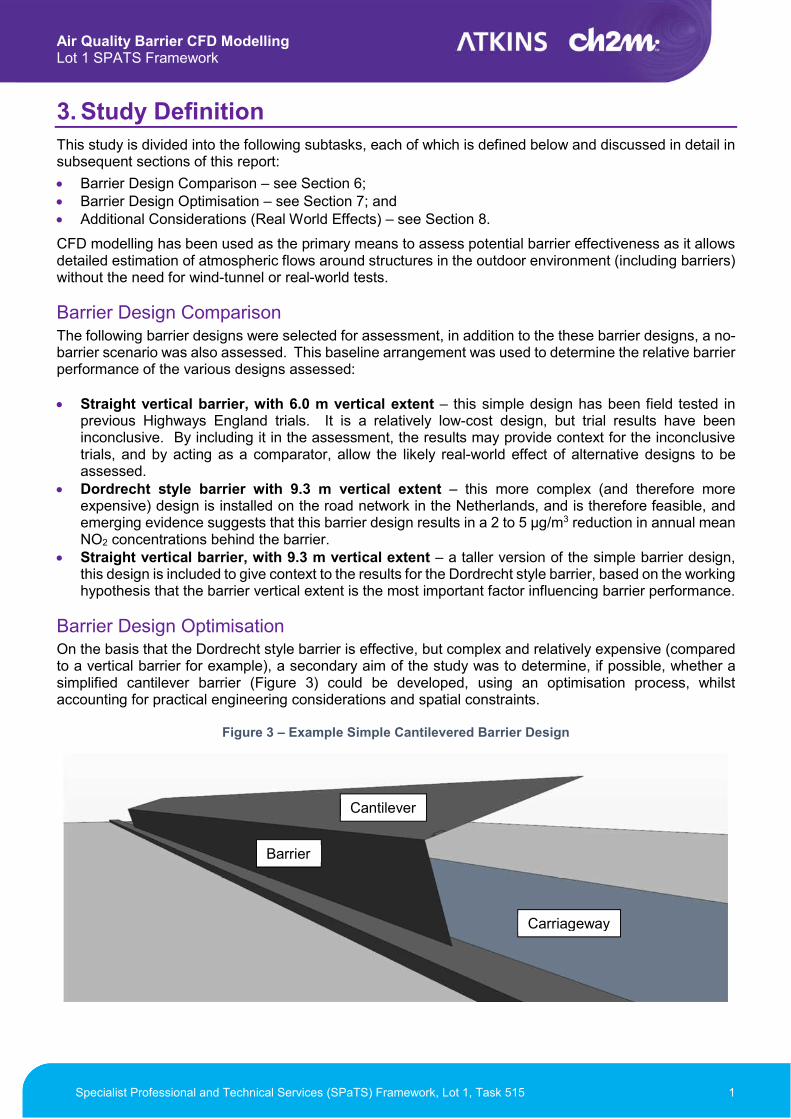
Barrier Design Optimisation On the basis that the Dordrecht style barrier is effective, but complex and relatively expensive (compared to a vertical barrier for example), a secondary aim of the study was to determine, if possible, whether a simplified cantilever barrier (Figure 3) could be developed, using an optimisation process, whilst accounting for practical engineering considerations and spatial constraints.
Figure 3 – Example Simple Cantilevered Barrier Design
Barrier
Cantilever
Carriageway

Air Quality Barrier CFD Modelling Lot 1 SPATS Framework
Specialist Professional and Technical Services (SPaTS) Framework, Lot 1, Task 515 2
Real World Factors The Barrier Design Comparison and optimisation tasks were both undertaken in a ‘generic’ idealised environment with a constant flow of traffic. They do not contain geometry which may influence dispersion, (such as adjacent buildings, cuttings and embankments or bridges and fly-overs), nor do they account for the influence that different traffic conditions may have on vehicle induced turbulence. These factors may affect overall barrier performance and therefore additional scenarios were considered to assess their influence. A tertiary objective of the study was therefore to better understand how ‘real-world’ factors, such as adjacent buildings, or different traffic conditions, could potentially influence the effectiveness of a barrier.
It is recognised that by its nature, steady state CFD modelling will not capture the unsteady fluctuations in the flow field and any resultant unsteadiness in pollutant concentrations. Steady state modelling is a practical necessity because of the very long duration and costly simulation effort required to perform the alternative. This is particularly true for studies involving optimisation and multiple simulation scenarios, such as this.
In order to assess the scale of any unsteadiness, to provide context to the steady state results and to illustrate its potential effect on barrier effectiveness, an alternative, more-detailed turbulence modelling approach is required, such as Large Eddy Simulation (LES), Detached Eddy Simulation (DES) or unsteady-Reynolds Averaged Navier Stokes (uRANS). LES is considered too computationally intensive for the timescales of the project. DES is a hybrid modelling approach that combines features of uRANS simulation in some parts of the flow and LES in others, and for this reason has been selected for this study.
Additional Wind Conditions A potential limitation of the analyses described above is that (as required by the initial scope of work) barrier performance was only evaluated under a single wind direction and wind speed. Additional analysis was therefore undertaken to confirm the above findings under alternative wind speeds and alternative wind directions.
As part of this additional work, further analysis was also undertaken to estimate the region behind the barrier over which barriers are likely to be most effective and any locations where pollutant concentrations may be increased as a result of the installation of a barrier. It was thought that this information could potentially inform a set of design principles for air quality barriers (e.g. “A barrier should extend XXm beyond sensitive receptors to maximise the effectiveness of the barrier” and/or “Increases in pollutant concentrations may potentially occur up to XXm beyond the end of a barrier”).
Air Quality Barrier CFD Modelling Lot 1 SPATS Framework
Specialist Professional and Technical Services (SPaTS) Framework, Lot 1, Task 515 3
4. CFD Modelling
Introduction Star-CCM+, an industry standard CFD code with advanced Computer Aided Design (CAD), mesh generation, turbulence and physics modelling capabilities, has been used exclusively on this project. The modelling was carried out using the steady state solver for the standalone barrier comparison and barrier optimisation activities, and the transient solver for the Detached Eddy Simulation (DES) modelling undertaken in the Real World Factors Task (see Section 8). The Star-CCM+ software package also includes optimisation tools and a large array of post-processing options and is therefore ideal for the barrier design optimisation activity.
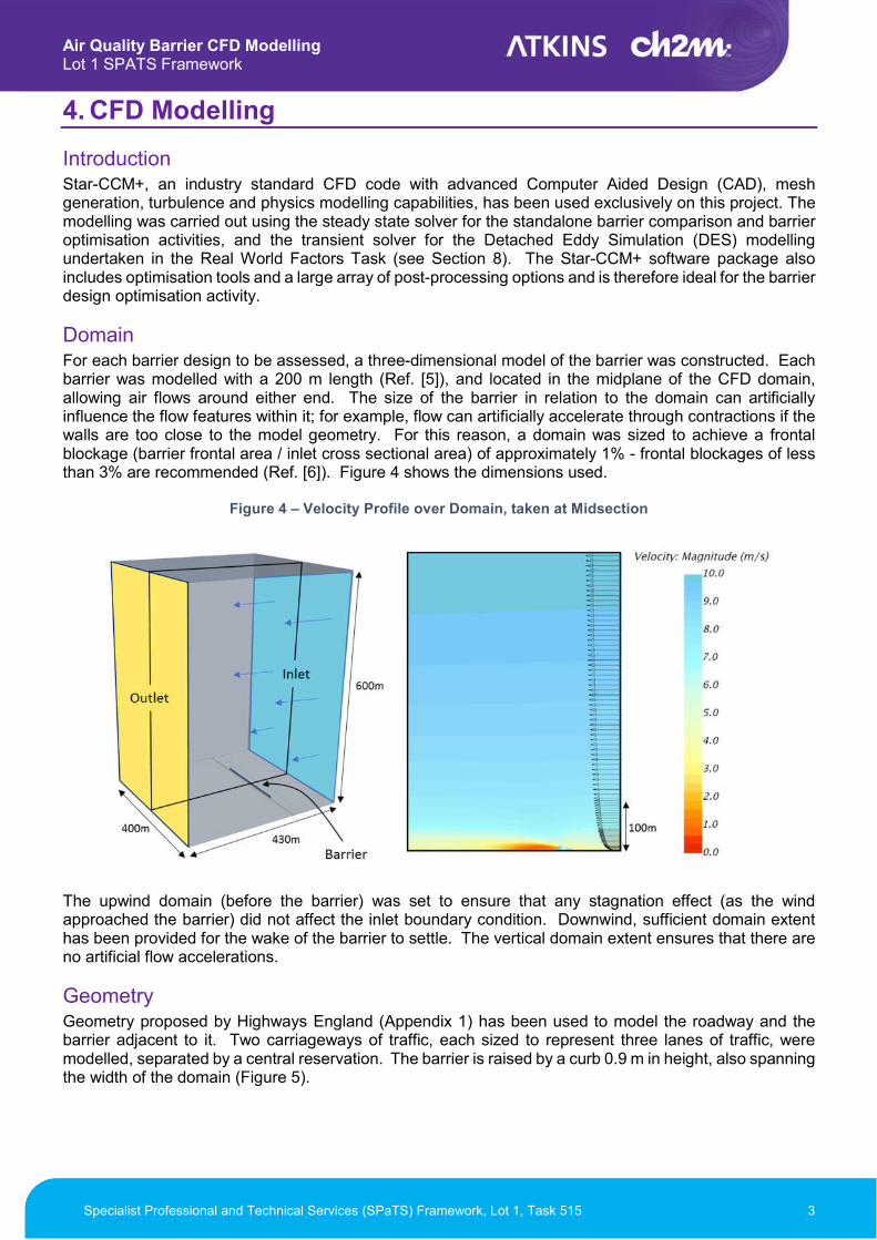
Domain For each barrier design to be assessed, a three-dimensional model of the barrier was constructed. Each barrier was modelled with a 200 m length (Ref. [5]), and located in the midplane of the CFD domain, allowing air flows around either end. The size of the barrier in relation to the domain can artificially influence the flow features within it; for example, flow can artificially accelerate through contractions if the walls are too close to the model geometry. For this reason, a domain was sized to achieve a frontal blockage (barrier frontal area / inlet cross sectional area) of approximately 1% - frontal blockages of less than 3% are recommended (Ref. [6]). Figure 4 shows the dimensions used.
Figure 4 – Velocity Profile over Domain, taken at Midsection
The upwind domain (before the barrier) was set to ensure that any stagnation effect (as the wind approached the barrier) did not affect the inlet boundary condition. Downwind, sufficient domain extent has been provided for the wake of the barrier to settle. The vertical domain extent ensures that there are no artificial flow accelerations.
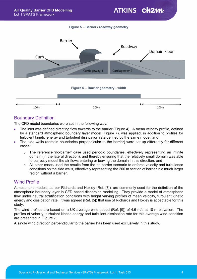
Geometry Geometry proposed by Highways England (Appendix 1) has been used to model the roadway and the barrier adjacent to it. Two carriageways of traffic, each sized to represent three lanes of traffic, were modelled, separated by a central reservation. The barrier is raised by a curb 0.9 m in height, also spanning the width of the domain (Figure 5).
Air Quality Barrier CFD Modelling Lot 1 SPATS Framework
Specialist Professional and Technical Services (SPaTS) Framework, Lot 1, Task 515 4
Figure 5 – Barrier / roadway geometry
Figure 6 – Barrier geometry - width
Boundary Definition The CFD model boundaries were set in the following way:
The inlet was defined directing flow towards to the barrier (Figure 4). A mean velocity profile, defined by a standard atmospheric boundary layer model (Figure 7), was applied, in addition to profiles for turbulent kinetic energy and turbulent dissipation rate defined by the same model; and
The side walls (domain boundaries perpendicular to the barrier) were set up differently for different cases:
o The reference ‘no-barrier’ case used periodic boundaries, effectively representing an infinite domain (in the lateral direction), and thereby ensuring that the relatively small domain was able to correctly model the air flows entering or leaving the domain in this direction; and
o All other cases used the results from the no-barrier scenario to enforce velocity and turbulence conditions on the side walls, effectively representing the 200 m section of barrier in a much larger region without a barrier.
Wind Profile Atmospheric models, as per Richards and Hoxley (Ref. [7]), are commonly used for the definition of the atmospheric boundary layer in CFD based dispersion modelling. They provide a model of atmospheric flow under neutral stratification conditions with height varying profiles of mean velocity, turbulent kinetic energy and dissipation rate. It was agreed (Ref. [5]) that use of Richards and Hoxley is acceptable for this study.
The wind profiles are based on a UK average wind speed (Ref. [9]) of 4.6 m/s at 10 m elevation. The profiles of velocity, turbulent kinetic energy and turbulent dissipation rate for this average wind condition are presented in Figure 7.
A single wind direction perpendicular to the barrier has been used exclusively in this study.

Air Quality Barrier CFD Modelling Lot 1 SPATS Framework
Specialist Professional and Technical Services (SPaTS) Framework, Lot 1, Task 515 5
Figure 7 – Atmospheric Boundary Layer
Traffic Modelling For the purposes of this study, two aspects of vehicular traffic must be considered: Forces: The impact of vehicle movement on the air flow is two-fold; changes to the velocity above the
carriageway and increases in turbulence levels. The impact can be modelled either explicitly, by modelling multiple moving vehicles with ‘overset’ meshes, or by applying source terms of momentum and turbulence to represent the induced flows. For the purposes of this study, it was considered not practical to explicitly model multiple moving vehicles and therefore the source term approach has been taken.
Emissions: Whilst pollutants are released from concentrated sources (i.e. the vehicle exhaust pipe),
vehicle movement and induced turbulence is highly effective at mixing these concentrated regions and pollutant concentrations rapidly homogenise (Ref. [5]). As a result, the pollutant source can be well represented by a uniform release over a larger volume above the carriageway (in this case, a volume source representing each carriageway, 6 metres in height and 10 metres in width).
Forces To correctly represent the traffic source term, two aspects must be considered: Vehicle Induced Momentum (VIM) and Vehicle Induced Turbulence (VIT). It is recognized that the turbulent energy comes from the energy lost by the vehicles and therefore is linked to the vehicular drag, which can be calculated. However, the split of energy between induced momentum in the near field and induced turbulence is not well researched. Despite substantial research having been undertaken in this area (Ref. [10], Ref. [11], Ref. [12]), there does not appear to be a consistent or universally agreed set of values for VIT. Furthermore, there is little evidence of researchers investigating VIM.
To implement the effects of vehicular movement in the barrier assessment CFD model, three parameters must be derived:
Induced velocity in the wake (% of traffic speed) Average Turbulent Kinetic Energy induced (J/kg) Turbulent Dissipation Rate (m2/s3)
Precursor CFD Model In lieu of published guidance on these three values, a precursor CFD model was constructed to model the actual traffic flows and extract their volume-averaged values. Typical traffic density and speed were proposed by Highways England, as per Table 1.

Air Quality Barrier CFD Modelling Lot 1 SPATS Framework
Specialist Professional and Technical Services (SPaTS) Framework, Lot 1, Task 515 6
Table 1 – Average Traffic Metrics
Parameter Value
Traffic density 140,000 vehicles/day = 0.54 vehicles/s/lane Traffic speed 62 mph (27.7 m/s) Vehicle spacing 51 m (calculated from traffic density) Height of passenger vehicle 1.5 m Height of HGV vehicle 4.0 m Percentage of HGV 10%
A CFD domain was created for a single carriageway (3 lanes) of traffic, including:
10 ‘stationary’ vehicles, spread across the three lanes including one HGV and nine passenger vehicles; and
Periodic inlet and outlet boundaries directing air at 62 mph (27.7 m/s) through the domain.
The CFD domain extent was sized to reduce artificial blockage effects. The model geometry, overlaid with a visualization of turbulent kinetic energy, is shown in Figure 8. The vertical and lateral extents of the vehicle wakes (shown in the figure) were used to define the averaging volume and barrier model source term volume. As a result, the cross-sectional area of the control volume chosen was 6 m x 10 m.
Figure 8 – Turbulent Kinetic Energy (TKE) visualised in CFD domain
The metrics of VIT and VIM were monitored within the control volume. The parameters derived for the 62 mph scenario were:
30% average Velocity Deficit (0.3 x traffic velocity); 3.02 J/kg average Turbulent Kinetic Energy; and 4.87 m2/s3 average Turbulent Dissipation Rate.
These values were subsequently used as source terms in traffic carriageway volumes for each of the barrier assessment CFD models. These volumes use the same cross-sectional area (6 m x 10 m) along the full width of the domain (400 m), as shown in Figure 9.
Traffic Emissions The primary purpose of the barrier assessment CFD model is to assess the dispersion of pollutant gases released from vehicles. The physical release process is understood to be as follows:
1. A vehicle releases emissions from its exhaust; 2. The vehicle induced turbulence mixes it with the air in the wake of the vehicle; 3. The vehicle induced momentum carries the emissions along the carriageway; 4. The wind entrains the emissions in the dominant wind direction; and 5. Emissions continue to dilute as they are carried downwind.
Pollutant Modelling Pollutant dispersion may be represented in the CFD model by active or passive scalars. Active scalars account for the density (and therefore buoyancy) of the released gas, this is important for the modelling of light or dense gas releases (lighter or heavier than air) and can also enable modelling of
Air Quality Barrier CFD Modelling Lot 1 SPATS Framework
Specialist Professional and Technical Services (SPaTS) Framework, Lot 1, Task 515 7
chemical reactions. Passive scalars may be considered as a release of inert, massless particles which are influenced by, but do not influence, the bulk flow (Ref. [13]).
Assuming that:
a) emissions are rapidly mixed and diluted by the vehicle induced turbulence and therefore concentrations evenly distributed along the carriageway;
b) no chemical reactions occur between the pollutant gas and the surrounding atmosphere; and c) the pollutants are of similar density to the surrounding air.
Then a passive scalar source term in the carriageway volume can be used to represent the physics of pollution release.
Whilst it is recognised that nitrogen monoxide (NO) emissions from road traffic react in the atmosphere to form nitrogen dioxide (NO2), the focus of this study has been on the relative effectiveness of different barrier designs, rather than the absolute effect on annual mean NO2 concentrations, for example. As a result, and as agreed with Highways England, passive scalars have been used to model pollutant dispersion in this study.
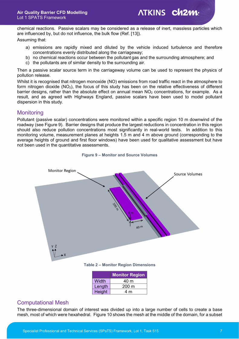
Monitoring Pollutant (passive scalar) concentrations were monitored within a specific region 10 m downwind of the roadway (see Figure 9). Barrier designs that produce the largest reductions in concentration in this region should also reduce pollution concentrations most significantly in real-world tests. In addition to this monitoring volume, measurement planes at heights 1.5 m and 4 m above ground (corresponding to the average heights of ground and first floor windows) have been used for qualitative assessment but have not been used in the quantitative assessments.
Figure 9 – Monitor and Source Volumes
Table 2 – Monitor Region Dimensions
Monitor Region
Width 40 m Length 200 m Height 4 m
Computational Mesh The three-dimensional domain of interest was divided up into a large number of cells to create a base mesh, most of which were hexahedral. Figure 10 shows the mesh at the middle of the domain, for a subset

Air Quality Barrier CFD Modelling Lot 1 SPATS Framework
Specialist Professional and Technical Services (SPaTS) Framework, Lot 1, Task 515 8
of the full domain in the region immediately adjacent to the barrier and downwind of it. A uniform cell size of approximately 10 m was applied to the majority of the domain, with a transition to progressively smaller cells close to the barrier. A small volume was defined around the barrier, filled with prismatic and trimmed cells (i.e. cells designed to match curved and complex shapes) to capture the trajectory of the pollution as accurately as possible. For the barrier designs simulated, the mesh comprised, on average, 2 million cells.
Figure 10 – Base Mesh with Blocked Refinement
Automated Mesh Adaption It is possible to refine the mesh in proportion to the concentration of Passive Scalar, a process known as Automated Mesh Adaption. Higher concentrations are expected close to the source and downwind of the barrier and so these regions are more likely to exhibit complex behaviour. A higher resolution mesh is better at capturing this and will improve concentration estimates in the monitoring region.
While this could be achieved with a high resolution mesh throughout the whole domain, it would be highly inefficient and, in the context, if these test scenarios would achieve similar results to running an Automated Mesh Adaption. Figure 11 shows a representative case where Automated Mesh Adaption has been applied. In this particular case, two levels of cell refinement have been used to accurately capture the pollutant concentration field.
Figure 11 – Base Mesh with Automated Mesh Adaption applied
Turbulence Model The CFD code solves the Reynolds-averaged equations for momentum, continuity, energy, turbulent kinetic energy and dissipation rate, using the realisable k-ε two equation closure model and 2nd order numerical schemes. Such modelling is routinely used in engineering for a wide variety of flows and has proved to be a mature and relatively robust tool.
Further detail on the Detached Eddy Simulation (DES) turbulence modelling undertaken as part of the ‘Real World Factors’ task is provided in Section 8.

Air Quality Barrier CFD Modelling Lot 1 SPATS Framework
Specialist Professional and Technical Services (SPaTS) Framework, Lot 1, Task 515 9
5. Barrier Performance
Introduction Three barrier designs are compared in this task: a 9.3 m Dordrecht style barrier, a 9.3 m vertical barrier and a 6 m vertical barrier (similar to that previously trialled by Highways England adjacent to the M62). All barriers were modelled with a con stant height along their full length, i.e. there was no feathering of the height down to ground level at their ends. A base case model was run without any barrier to act as a benchmark, allowing improvements in pollutant concentration to be quantified.
For each of the modelled scenarios the passive scalar results were plotted on planar surface ‘sections’, as follows:
A vertical section through the centreline of the domain, parallel with the wind direction; A horizontal section at 1.5 m elevation, parallel with the ground; and A horizontal section at 4.0 m elevation, parallel with the ground.
Figure 12 shows an illustration of the vertical and horizontal section planes on which results are plotted from each simulation.
Figure 12 – Sections taken of the domain (for illustration only)

Air Quality Barrier CFD Modelling Lot 1 SPATS Framework
Specialist Professional and Technical Services (SPaTS) Framework, Lot 1, Task 515 10
No Barrier Case A vertical section along the midplane of the domain for the no barrier case domain is shown in Figure 13. Horizontal sections are shown in Figure 14.
Figure 13 – Elevation View of the No Barrier Case
Figure 14 – Plan View of the No Barrier Case at 1.5 m (left) and 4 m (right)
The results indicate that:
a) the atmospheric boundary layer both carries the pollution downwind away from the carriageway and dilutes it by mixing,
b) Concentrations at 1.5 m height (Figure 14 b(i)) are greater than the concentrations at 4 m (Figure 14 b(ii)).

Air Quality Barrier CFD Modelling Lot 1 SPATS Framework
Specialist Professional and Technical Services (SPaTS) Framework, Lot 1, Task 515 11
Dordrecht Barrier A vertical and horizontal section of the Dordrecht barrier case are shown in Figure 15 and Figure 16 respectively, with specific features of interest (labelled a to e) discussed further below.
Figure 15 - Elevation View of the Dordrecht Barrier Case
Figure 16 - Plan View of the No Barrier Case at 1.5 m (left) and Dordrecht Barrier at 1.5 m (right)
The results indicate that:
a) The large containment volume, due to the long, cantilevered overhang of the barrier, causes pollution to accumulate along the roadway;
b) The ‘blocking’ effect of the barrier forces flow upwards, dispersing pollutants over a larger area; c) A recirculation zone develops behind the barrier in which the pollutants that have been forced
upwards are recirculated back down into the monitoring volume; d) In the roadway, traffic momentum pulls the pollution captured behind the barrier in the direction of
travel. This flow is ejected on the far side of the barrier and away from the monitor region, creating the asymmetry seen in Figure 16; and
e) The traffic momentum also directs flow (and emissions) from the road behind the barrier, into the monitor region.

Air Quality Barrier CFD Modelling Lot 1 SPATS Framework
Specialist Professional and Technical Services (SPaTS) Framework, Lot 1, Task 515 12
The volume average of pollution observed in the monitoring region downwind of the Dordrecht barrier was lower than the no-barrier base case by 36%. Spatial variations in barrier performance within the monitoring region are discussed in Section 6, with values illustrated in Table 4.
It should be remembered however that this modelled difference in concentration relates only to a particular set of meteorological conditions (i.e. a constant wind speed perpendicular to the barrier) and not, for example, the reduction in the annual average concentration in the monitoring region. Measurements undertaken by Highways England behind a similar barrier in Holland do however indicate that such a barrier design is effective in reducing annual mean concentrations, and therefore that a barrier which is modelled to result in a reduction in concentration of the magnitude described above has the potential to have an observable effect on annual mean concentrations in the real-world.
Vertical Barrier – 9.3 m A vertical and horizontal section of the straight vertical 9.3 m barrier case are shown in Figure 17 and Figure 18 respectively, with specific features of interest (labelled a to e) discussed further below.
Figure 17 - Elevation View of the Straight 9.3 m case
Figure 18 - Plan View of the No Barrier Case at 1.5 m (left) and Straight 9.3 m Barrier at 1.5 m (right)

Air Quality Barrier CFD Modelling Lot 1 SPATS Framework
Specialist Professional and Technical Services (SPaTS) Framework, Lot 1, Task 515 13
The results indicate that:
a) Without any overhang, less of the pollutant is contained. Air with higher concentrations of pollutant is drawn over the barrier and into the downwind recirculation region;
b) The incoming wind impinges on the barrier wall and is pushed upward at a steep angle and mixes with air flow above the barrier. As a result of this increased vertical mixing, the pollutants are spread over a greater vertical range than the Dordrecht style barrier;
c) The downwind recirculation draws flow ejected over the barrier back into the monitoring region; d) The traffic momentum pulls the pollution captured behind the barrier in the direction of travel, but
also directs flow behind the barrier, into the monitor region.
The volume average of Passive Scalar observed in the monitoring region downwind of the 9.3 m vertical barrier was lower than the no-barrier base case by 39%, giving a very similar performance to the Dordrecht style barrier. Spatial variations in barrier performance within the monitoring region are discussed in Section 6, with values illustrated in Table 4.
Vertical Barrier – 6.0 m A vertical and horizontal section of the straight vertical 6.0 m barrier case are shown in Figure 19 and Figure 20 respectively, with specific features of interest (labelled a to c) discussed further below.
The results indicate that:
a) With a smaller (6.0 m) barrier to prevent spill over, lower levels of pollutant are contained roadside of the barrier than for the 9.3 m barrier;
b) The incoming wind impinges on the barrier wall, but due to the lower barrier height, it is pushed upward at a shallower angle and does not promote as much mixing with air flow above the barrier as the 9.3 m barrier. The air is deflected less because a) the shorter barrier height results in less blockage of the wind (the barrier surface area is smaller by 6.0 / 9.3) and therefore a smaller mass flow of air is flowing over the top of the barrier and b) because the air that is deflected by the barrier has to turn through a greater angle to get over the top. These two effects mean that the flow over the top of the shorter barrier has less momentum and a smaller vertical component.
c) As this deflected polluted flow is straightened downwind it mixes in a recirculation zone. A smaller recirculation zone is formed for the shorter barrier. This shorter height recirculation reduces the total quantity of fresh incoming air that the barrier can mix (dilute the pollutants) with, and the overall performance of the shorter barrier is lower.
The volume average of pollution observed in the monitoring region downwind of the 6.0 m vertical barrier was lower than the no-barrier base case by 19%. Spatial variations in barrier impact are discussed in Section 6, with values illustrated in Table 4.
It should be remembered however that this modelled difference in concentration relates only to a particular set of meteorological conditions (i.e. a constant wind speed perpendicular to the barrier) and not, for example, the reduction in the annual average concentration in the monitoring region. Measurements undertaken by Highways England behind a barrier of similar height adjacent to the M62 were inconclusive, suggesting that a barrier which is modelled to result in a reduction in concentration of the magnitude described above is unlikely to have an observable effect on annual mean concentrations in the real-world.

Air Quality Barrier CFD Modelling Lot 1 SPATS Framework
Specialist Professional and Technical Services (SPaTS) Framework, Lot 1, Task 515 14
Figure 19 - Elevation View of the Straight 6.0 m Barrier
Figure 20 - Plan View of the No Barrier Case at 1.5 m (left) and Straight 6.0 m Barrier at 1.5 m (right)

Air Quality Barrier CFD Modelling Lot 1 SPATS Framework
Specialist Professional and Technical Services (SPaTS) Framework, Lot 1, Task 515 15
6. Barrier Comparison
The barrier designs are compared in the following ways in this section:
1. Absolute performance (volume average concentration values within the monitoring region); 2. Relative performance (for the same volume average) compared to the no-barrier case; 3. Concentrations at a transect of monitor points perpendicular to the midpoint of the barrier; and 4. Concentration distribution over the monitoring volume, presented as a histogram.
Performance
Table 3 provides a summary of the performance results, both in terms of the absolute value and relative reduction from the no-barrier case, for each barrier design. The percentage reductions included here are a repeat of those in the text of the previous section.
Table 3 – Summary of Results for Standalone Cases
No Barrier Dordrecht
Barrier Straight 9.3 m
Barrier Straight 6.0 m
Barrier Volume Average
Concentration 3.07 1.95 1.88 2.48
Percentage reduction
- 36% 39% 19%
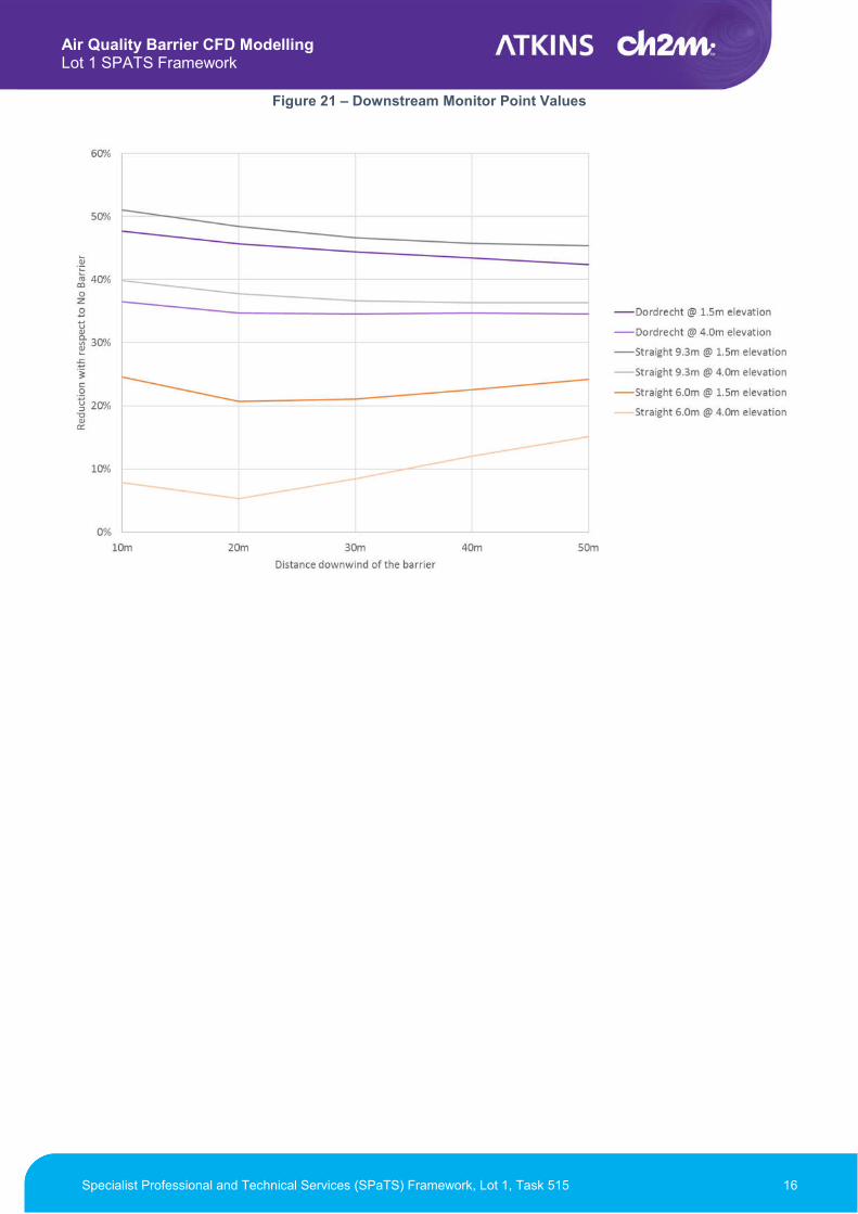
Monitor Point Transects A total of ten monitor points, five at 1.5 m elevation and five at 4 m elevation, were set at 10 m intervals between 10 m and 50 m downwind of and perpendicular to the mid-point of the barrier. The percentage reduction in concentration at each of these monitor points (relative to the no-barrier base case) is shown in Table 4 and Figure 21.
Table 4 – Downstream Monitor Point – Percentage Reductions
10 m 20 m 30 m 40 m 50 m
Dordrecht Barrier
1.5 m 48% 46% 44% 43% 42%
4.0 m 36% 35% 35% 35% 35%
Straight 9.3 m Barrier
1.5 m 51% 48% 47% 46% 45%
4.0 m 40% 38% 37% 36% 36%
Straight 6.0 m Barrier
1.5 m 25% 21% 21% 23% 24%
4.0 m 8% 5% 8% 12% 15%
The results indicate that the largest concentration reductions are for monitor points at 1.5 m elevation, with improvements at this elevation greater than those at 4 m elevation for all designs. The results also reiterate the fact that the 9.3 m barrier designs outperform the 6.0 m barrier at both measurement point elevations. The overall trend is also in line with the volume-averaged result.
Air Quality Barrier CFD Modelling Lot 1 SPATS Framework
Specialist Professional and Technical Services (SPaTS) Framework, Lot 1, Task 515 16
Figure 21 – Downstream Monitor Point Values

Air Quality Barrier CFD Modelling Lot 1 SPATS Framework
Specialist Professional and Technical Services (SPaTS) Framework, Lot 1, Task 515 17
7. Optimisation
Introduction A cantilevered barrier, comparable to a simplified Dordrecht shape, could be easier to manufacture and install than the Dordrecht design and therefore more cost effective to roll-out more widely. The best performing design of such a barrier can be found with an optimisation study.
This section details the results, methodology and consequences of the optimisation study carried out on the cantilevered barrier.
Optimisation Procedure An optimisation procedure has several key steps, listed below:
1. Model Build: creating a parameterised CFD model and applying constraints;
2. Objectives: defining a value to minimise (in this case, pollutant concentration);
3. Simulation/Optimisation: identifying the best performing model; and
4. Post-Processing: understanding the sensitivity of the best design to perturbations.
Optimisation Methodology Star-CCM+ has a range of tools to identify the best performing design in a set. The simplest runs every possible design within a given space; the more intelligent uses algorithms that search for the best design. The latter approach was chosen for this study as: total run time can be reduced, as fewer simulations are required to be run; a wide range of design types can be trailed; and the variable driving the best design can be identified. The local Star-CCM+ optimiser “SHERPA” is such an algorithm and was chosen due to its intelligent features, convenience, and extensive user support available in the event of technical difficulties. The results of the optimisation using SHERPA are discussed in the following sections.
Geometry Parameterisation The cantilevered design was modelled using the two-node parameterised geometry shown in Figure 22. The vertical and horizontal extents of each node define the realistic limits of building the barrier next to a roadway; these were agreed with Highways England before running the study. The same traffic and wind conditions were used in the optimisation simulations as were used in the standalone cases to allow a direct comparison to be made.

Air Quality Barrier CFD Modelling Lot 1 SPATS Framework
Specialist Professional and Technical Services (SPaTS) Framework, Lot 1, Task 515 18
Figure 22 – Parameterised Cantilevered Geometry
Results A total of 50 designs were simulated before an optimal design was reached, providing one best design, one worst design and 48 intermediary designs. Figure 23 shows every design variation simulated, highlighting the best and worst designs for comparison. The figure also includes the Dordrecht and straight barrier geometries, for reference. Table 5 shows the absolute results.
Figure 23 – Designs run in the optimisation study

Air Quality Barrier CFD Modelling Lot 1 SPATS Framework
Specialist Professional and Technical Services (SPaTS) Framework, Lot 1, Task 515 19
Table 5 – Results of Optimisation Study
No Barrier Dordrecht
Design
Vertical barrier
(9.3 m)
Best Design
(see figure above)
Worst Design
(9.3 m)
Worst Design
(Overall)
Absolute Value
3.07 1.95 1.88 1.94 2.16 2.4
Percentage Reduction
- 36% 39% 37% 26% 21%
Discussion
It is noted that the shapes of the best and worst designs are significantly different. As the best design approximates a straight barrier, this indicates that barrier performance is greatest when:
the total height is maximised; the overhang length is minimised; and the containment volume is minimised.
Further analysis indicates that the way the wind and traffic induced flows interact with the designs can substantially affect pollutant concentrations in the monitor region. The key flow features and their implications are discussed in the following section.
Key Flow Features
Figure 24 shows the concentration distribution seen for a typical cantilevered barrier, with specific features of interest (labelled a to c) discussed further below.
For the specific environment modelled, the pollutant concentration in the downwind region is the result of three key aerodynamic phenomena:
a) Traffic induced momentum entraining flow behind the barrier in the traffic direction; b) Pollution forced along the roadway, accumulating and spilling over the top of the barrier; and c) Downwind recirculation drawing pollution back into the monitor region.

Air Quality Barrier CFD Modelling Lot 1 SPATS Framework
Specialist Professional and Technical Services (SPaTS) Framework, Lot 1, Task 515 20
Figure 24 – Key Flow Features of Cantilevered Barrier
Design Features Influencing Barrier Performance
For the barrier designs approximating a straight barrier (short overhang, high bottom section), the air forced behind the barrier by the traffic induced momentum maintains a higher velocity. This causes a ‘drawback’ effect, bringing the pollution towards the barrier, out of the monitor region. A comparison of the concentrations distribution for the ‘best’ performing design and the ‘worst’ performing design is shown in Figure 25, with specific features of interest (labelled a to d) discussed further below.

Air Quality Barrier CFD Modelling Lot 1 SPATS Framework
Specialist Professional and Technical Services (SPaTS) Framework, Lot 1, Task 515 21
Figure 25 – Best Design (top) vs Worst Design (bottom) Concentrations
As shown in Figure 25:
a) Airflow is directed higher off the straight edge; b) High vehicle induced momentum close to the barrier draws pollutants back towards the barrier; and c) A zone of low concentration emerges at the centre of the barrier.
The ‘worst’ performing designs have a large overhang. For these designs, wind flowing over the barrier remains attached to the overhang section and is pulled into the recirculation region (Figure 25, d), and prevents the momentum behind the barrier being maintained (Figure 25, a), eliminating the beneficial ‘drawback’ effect.
In summary, there are performance benefits associated with straight barriers, whilst the presence of traffic induced momentum appears to reduce the beneficial containment effect provided by a cantilevered section. This issue is investigated further in Section 8.
Relative performance
In order to understand the magnitude of the difference in the potential effectiveness of the ‘best’ and ‘worst barrier designs, the relative performance of each design has been considered. Figure 26 shows the total reduction in pollutant concentration (y-axis) compared to the no-barrier case for its maximum height (x-axis), for each design assessed by the optimiser. The following can be seen:
There is a general benefit gained in pollution reduction with overall barrier height, but at any given height the barrier shape is important.
Cantilevered barriers at the maximum allowed height (9.3 m) can perform worse than better designed barriers with lower overall height.
For barriers at the maximum allowed height, the difference in pollutant reduction between the best and worst designs is approximately 8%, but the difference between the best cantilever geometry (the Dordrecht design) and a straight barrier is insignificant.
It follows that a simple straight design, modelled at a 62mph average traffic velocity and at 9.3 m in height, has both performance benefits and the advantage of maximum height. A cantilever barrier, which could potentially offer performance benefits at lower traffic velocities (see Section 8), will be more complex to construct for limited performance enhancements.

Air Quality Barrier CFD Modelling Lot 1 SPATS Framework
Specialist Professional and Technical Services (SPaTS) Framework, Lot 1, Task 515 22
Figure 26 – Optimisation Study Percentage Reduction in Volume Average vs. Maximum Height
Modelling Environment
The results from the optimisation study clearly show that traffic momentum potentially has a major influence on the effectiveness of a barrier. The sensitivity to a change in average traffic velocity is also high; for example, a 10 mph reduction can lead to a very different optimum design. The wind profile and traffic momentum impinging on the barrier is complex and three-dimensional, making it hard to pinpoint a single optimal design for the many environmental conditions experienced in ‘real life’.
Whilst the modelling undertaken as part of this study makes use of an idealised environment to enable different designs to be visualised and compared, there are a number of factors which could potentially influence the outcome of an optimisation study in the ‘real world’. These include:
1. The traffic momentum drives much of the pollutant volume behind the barrier and into the monitor region: any physical disruption (trees, buildings etc) in the gap between the edge of the domain and the barrier may reduce this effect considerably;
2. Buildings in the monitor region may affect downwind and crosswind airflow behind the barrier affecting pollution concentrations;
3. Different wind conditions, such as oblique angles and speeds, may influence the overall distribution of pollution (this is unlikely as the wind velocity is low relative to the traffic); and
4. The average traffic velocity is assumed to be 62mph: the barrier may perform differently given alternative, or zero, momentum conditions.
Some of these factors are addressed in the following section.
Air Quality Barrier CFD Modelling Lot 1 SPATS Framework
Specialist Professional and Technical Services (SPaTS) Framework, Lot 1, Task 515 23
8. Additional considerations (Real World Effects)
Introduction ‘Real world’ effects, those not simulated in the idealised CFD model, have the potential to alter the performance of a barrier design. The following ‘real world’ effects were assessed:
1. Traffic at standstill; 2. A building in the lee of the barrier; and 3. Unsteady turbulent dispersion.
The results of these investigations are discussed below.
Traffic at Standstill Modelling
Each standalone case from Task 2 was replicated and re-run with no momentum source term in the roadway volumes. Both the pollution release rate and the wind direction were set to the same specification as the standalone cases.
Results
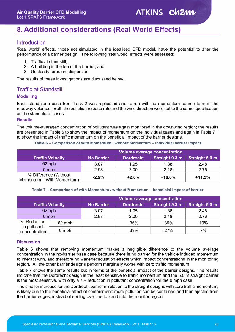
The volume-averaged concentration of pollutant was again monitored in the downwind region; the results are presented in Table 6 to show the impact of momentum on the individual cases and again in Table 7 to show the impact of traffic momentum on the beneficial impact of the barrier designs.
Table 6 – Comparison of with Momentum / without Momentum – individual barrier impact
Volume average concentration
Traffic Velocity No Barrier Dordrecht Straight 9.3 m Straight 6.0 m
62mph 3.07 1.95 1.88 2.48
0 mph 2.98 2.00 2.18 2.76 % Difference (Without
Momentum – With Momentum) -2.9% +2.6% +16.0% +11.3%
Table 7 – Comparison of with Momentum / without Momentum – beneficial impact of barrier
Volume average concentration
Traffic Velocity No Barrier Dordrecht Straight 9.3 m Straight 6.0 m
62mph 3.07 1.95 1.88 2.48
0 mph 2.98 2.00 2.18 2.76 % Reduction in pollutant
concentration
62 mph - -36% -39% -19%
0 mph - -33% -27% -7%
Discussion
Table 6 shows that removing momentum makes a negligible difference to the volume average concentration in the no-barrier base case because there is no barrier for the vehicle induced momentum to interact with, and therefore no wake/recirculation effects which impact concentrations in the monitoring region. All the other barrier designs perform marginally worse with zero traffic momentum.
Table 7 shows the same results but in terms of the beneficial impact of the barrier designs. The results indicate that the Dordrecht design is the least sensitive to traffic momentum and the 6.0 m straight barrier is the most sensitive, with only a 7% reduction in pollutant concentration for the 0 mph case.
The smaller increase for the Dordrecht barrier in relation to the straight designs with zero traffic momentum, is likely due to the beneficial effect of containment: more pollution can be contained and then ejected from the barrier edges, instead of spilling over the top and into the monitor region.

Air Quality Barrier CFD Modelling Lot 1 SPATS Framework
Specialist Professional and Technical Services (SPaTS) Framework, Lot 1, Task 515 24
However, given the frequency of complete traffic standstill is small in comparison to the frequency of traffic in motion, the beneficial effects of a barrier with an overhang are likely to be mostly negated. Therefore, a simple straight barrier at maximum height should still be considered as the most cost-effective design.
Figure 27 – No Momentum (above) vs With momentum (below)
Figure 28 - With Momentum (left) vs. No Momentum (right)
Air Quality Barrier CFD Modelling Lot 1 SPATS Framework
Specialist Professional and Technical Services (SPaTS) Framework, Lot 1, Task 515 25
A Building in the Lee of the Barrier Modelling
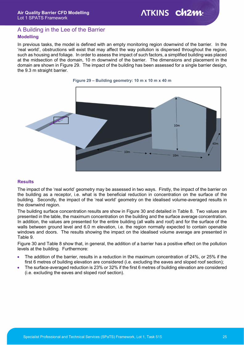
In previous tasks, the model is defined with an empty monitoring region downwind of the barrier. In the ‘real world’, obstructions will exist that may affect the way pollution is dispersed throughout the region, such as housing and foliage. In order to assess the impact of such factors, a simplified building was placed at the midsection of the domain, 10 m downwind of the barrier. The dimensions and placement in the domain are shown in Figure 29. The impact of the building has been assessed for a single barrier design, the 9.3 m straight barrier.
Figure 29 – Building geometry: 10 m x 10 m x 40 m
Results
The impact of the ‘real world’ geometry may be assessed in two ways. Firstly, the impact of the barrier on the building as a receptor, i.e. what is the beneficial reduction in concentration on the surface of the building. Secondly, the impact of the ‘real world’ geometry on the idealised volume-averaged results in the downwind region.
The building surface concentration results are show in Figure 30 and detailed in Table 8. Two values are presented in the table, the maximum concentration on the building and the surface average concentration. In addition, the values are presented for the entire building (all walls and roof) and for the surface of the walls between ground level and 6.0 m elevation, i.e. the region normally expected to contain openable windows and doors. The results showing the impact on the idealised volume average are presented in Table 9.
Figure 30 and Table 8 show that, in general, the addition of a barrier has a positive effect on the pollution levels at the building. Furthermore:
The addition of the barrier, results in a reduction in the maximum concentration of 24%, or 25% if the first 6 metres of building elevation are considered (i.e. excluding the eaves and sloped roof section);
The surface-averaged reduction is 23% or 32% if the first 6 metres of building elevation are considered (i.e. excluding the eaves and sloped roof section).

Air Quality Barrier CFD Modelling Lot 1 SPATS Framework
Specialist Professional and Technical Services (SPaTS) Framework, Lot 1, Task 515 26
Figure 30 – Surface Concentrations for the 9.3 m Straight Barrier Design - No Barrier (left) vs Straight 9.3 m Barrier (right)
Table 8 – Surface Concentrations Recorded on the Building – With and without the 9.3 m Straight Barrier
Entire Building Walls 0 m - 6 m
Design Surface Average Maximum Surface Average Maximum
No Barrier 2.90 3.93 2.99 3.93
Straight (9.3 m) 2.24 3.00 2.03 2.95
Percentage Difference
-23% -24% -32% -25%
Figure 31 and Table 9 show that the presence of the building alters the volume-averaged concentrations and indicates a reduction in the benefit of the barrier compared to the idealised no-building scenario. The contour plot in the figure indicates that the building disrupts the large recirculation downwind of the barrier and draws the high concentrations down to a lower level.
Figure 31 – Concentrations within Monitoring Region for the 9.3 m Straight Barrier Design - No Building (above) vs With Building (below)

Air Quality Barrier CFD Modelling Lot 1 SPATS Framework
Specialist Professional and Technical Services (SPaTS) Framework, Lot 1, Task 515 27
Table 9 – Volume Average Concentrations within Monitoring Region
Volume average concentration
Design No building With building
No Barrier 3.07 2.83
Straight (9.3 m) 1.88 1.95
Percentage Difference
-39% -31%
NB1: the volume average concentration reduction due to the introduction of the barrier is also lessened because the building acts in a similar manner as the barrier and provides increased mixing of pollutants for the base case.
NB2: The volume average assessment does not pick up the high concentrations on the front face of the building as the volume is blocked by the building itself.
Time-varying Dispersion The assessments of barrier performance presented so far in this study used averaged results from steady state simulation. By its nature this type of modelling does not capture unsteady physical behaviours, such as the unsteadiness in the wake of a barrier. In order to assess the scale of any unsteadiness, and its potential effect on barrier effectiveness, an alternative turbulence modelling approach is required. Direct Eddy Simulation (DES) was chosen to assess the unsteady behaviour for the Straight 9.3 m barrier.
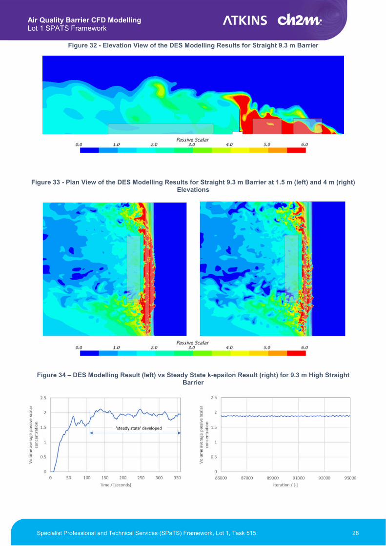
The results from the DES modelling are presented as contour plots in Figure 32 and Figure 33 and the time varying nature is indicated in the traces of Figure 34. The contour plots present similar views to those for the steady state modelling (Figure 17, Figure 18), and similar overall behaviours in the flow, but with more small scale variation in the pollutant concentrations. The fluctuations in the volume-averaged concentration (the key value used throughout the study) can be seen in Figure 34 for the 9.3 m straight barrier case. The plot indicates a 10% variation in the volume averaged result. The time average of this fluctuating result has similar magnitude to the steady state result.
The DES modelling indicates relatively good matching to the overall results from the steady simulations.
Air Quality Barrier CFD Modelling Lot 1 SPATS Framework
Specialist Professional and Technical Services (SPaTS) Framework, Lot 1, Task 515 28
Figure 32 - Elevation View of the DES Modelling Results for Straight 9.3 m Barrier
Figure 33 - Plan View of the DES Modelling Results for Straight 9.3 m Barrier at 1.5 m (left) and 4 m (right) Elevations
Figure 34 – DES Modelling Result (left) vs Steady State k-epsilon Result (right) for 9.3 m High Straight Barrier

Air Quality Barrier CFD Modelling Lot 1 SPATS Framework
Specialist Professional and Technical Services (SPaTS) Framework, Lot 1, Task 515 29
9. Additional Wind Conditions
Introduction In order to confirm that the relative performance of the different barrier designs considered above is similar under different wind conditions, rather than just specific to the single wind conditions considered in the previous sections, additional modelling work has been carried out to assess the performance of the two 9.3 m high barrier designs (Dordrecht and vertical) under a number of different wind directions and wind speeds. The results of this additional modelling work are presented in this section.
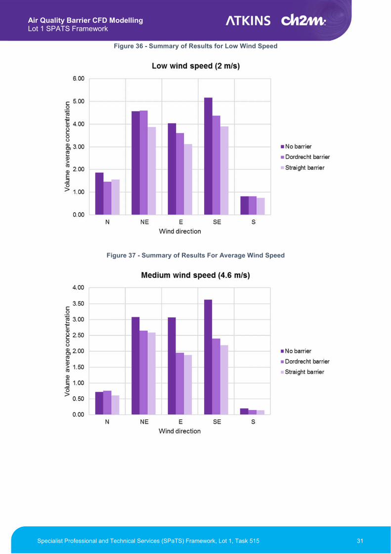
Scenarios Considered Figure 35 shows the wind directions considered within the additional modelling. Wind speeds of 2 m/s (low), 4.6 m/s (average) and 6 m/s (high) have been modelled for each wind direction. For comparison, the wind condition considered in Section 6 is an easterly wind at 4.6 m/s.
Figure 35 - Wind directions considered for additional modelling work (the lanes of traffic and monitoring region are shown in light grey)
Results Table 10 shows the volume average pollutant concentration for each modelled scenario, as well as the reduction in pollutant concentration against the no barrier case. These results are presented graphically in Figure 36 to Figure 38.

Air Quality Barrier CFD Modelling Lot 1 SPATS Framework
Specialist Professional and Technical Services (SPaTS) Framework, Lot 1, Task 515 30
Table 10 – Summary of Results for Additional Wind Scenarios
Wind direction
Wind speed (m/s)
Volume average concentration Percentage change
No barrier Dordrecht
barrier Straight 9.3 m barrier
Dordrecht barrier
Straight 9.3 m barrier
N 2 1.87 1.46 1.56 -22% -17%
4.6 0.72 0.76 0.61 5% -15%
6 0.47 0.53 0.37 11% -23%
NE 2 4.57 4.59 3.87 0% -15%
4.6 3.08 2.65 2.59 -14% -16% 6 2.72 1.99 2.18 -27% -20%
E 2 4.03 3.61 3.12 -10% -23%
4.6 3.07 1.95 1.88 -36% -39% 6 2.36 1.28 1.65 -46% -30%
SE 2 5.16 4.37 3.89 -15% -25%
4.6 3.63 2.40 2.19 -34% -40% 6 2.89 1.76 1.71 -39% -41%
S 2 0.83 0.82 0.76 -1% -8%
4.6 0.20 0.15 0.14 -25% -30% 6 0.13 0.09 0.09 -31% -31%
These results indicate that:
The lower the wind speed, the higher the pollutant concentration in the monitoring region for all wind directions.
The NE, E and SE wind directions result in higher pollutant concentrations in the monitoring regions than N and S wind directions for all wind speeds.
For the low and medium wind speeds, the straight barrier outperformed the Dordrecht barrier for NE, E and SE winds.
For the high wind speed, the Dordrecht barrier outperformed the straight barrier for NE and E wind directions, but the two barriers perform similarly for the SE wind direction.
The pollutant concentration in the monitoring region is much lower for the N and S wind directions, therefore the relative performance of the two barrier designs is less significant for these cases.
Air Quality Barrier CFD Modelling Lot 1 SPATS Framework
Specialist Professional and Technical Services (SPaTS) Framework, Lot 1, Task 515 31
Figure 36 - Summary of Results for Low Wind Speed
Figure 37 - Summary of Results For Average Wind Speed
Air Quality Barrier CFD Modelling Lot 1 SPATS Framework
Specialist Professional and Technical Services (SPaTS) Framework, Lot 1, Task 515 32
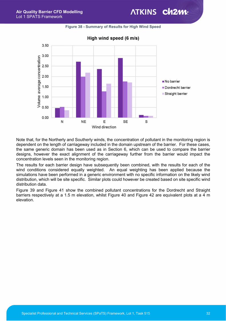
Figure 38 - Summary of Results for High Wind Speed
Note that, for the Northerly and Southerly winds, the concentration of pollutant in the monitoring region is dependent on the length of carriageway included in the domain upstream of the barrier. For these cases, the same generic domain has been used as in Section 6, which can be used to compare the barrier designs, however the exact alignment of the carriageway further from the barrier would impact the concentration levels seen in the monitoring region.
The results for each barrier design have subsequently been combined, with the results for each of the wind conditions considered equally weighted. An equal weighting has been applied because the simulations have been performed in a generic environment with no specific information on the likely wind distribution, which will be site specific. Similar plots could however be created based on site specific wind distribution data.
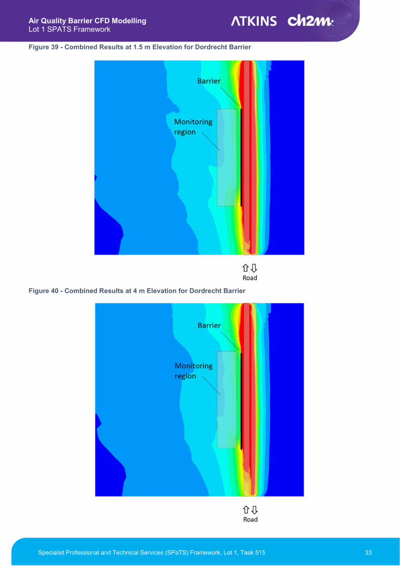
Figure 39 and Figure 41 show the combined pollutant concentrations for the Dordrecht and Straight barriers respectively at a 1.5 m elevation, whilst Figure 40 and Figure 42 are equivalent plots at a 4 m elevation.
Air Quality Barrier CFD Modelling Lot 1 SPATS Framework
Specialist Professional and Technical Services (SPaTS) Framework, Lot 1, Task 515 33
Figure 39 - Combined Results at 1.5 m Elevation for Dordrecht Barrier
Figure 40 - Combined Results at 4 m Elevation for Dordrecht Barrier

Air Quality Barrier CFD Modelling Lot 1 SPATS Framework
Specialist Professional and Technical Services (SPaTS) Framework, Lot 1, Task 515 34
Figure 41 - Combined Results at 1.5 m Elevation for Straight Barrier
Figure 42 - Combined Results at 4 m Elevation for Straight Barrier

Air Quality Barrier CFD Modelling Lot 1 SPATS Framework
Specialist Professional and Technical Services (SPaTS) Framework, Lot 1, Task 515 35
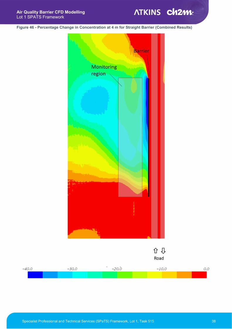
Edge Effects In order to assess the performance of each of the barrier designs near the ends of the barrier (referred to herein as “edge effects”), the percentage change in pollutant concentration compared to the ‘no barrier’ case has been calculated using the combined results for each of the barriers described above. These percentage change results are shown in Figure 43 to Figure 46, with the red colour representing no beneficial impact and blue representing the greatest positive impact.
Figure 43 - Percentage Change in Concentration at 1.5 m Elevation for Dordrecht Barrier (Combined Results)

Air Quality Barrier CFD Modelling Lot 1 SPATS Framework
Specialist Professional and Technical Services (SPaTS) Framework, Lot 1, Task 515 36
Figure 44 - Percentage Change in Concentration at 4 m Elevation for Dordrecht Barrier (Combined Results)

Air Quality Barrier CFD Modelling Lot 1 SPATS Framework
Specialist Professional and Technical Services (SPaTS) Framework, Lot 1, Task 515 37
Figure 45 - Percentage Change in Concentration at 1.5 m Elevation for Straight Barrier (Combined Results)
Air Quality Barrier CFD Modelling Lot 1 SPATS Framework
Specialist Professional and Technical Services (SPaTS) Framework, Lot 1, Task 515 38
Figure 46 - Percentage Change in Concentration at 4 m for Straight Barrier (Combined Results)

Air Quality Barrier CFD Modelling Lot 1 SPATS Framework
Specialist Professional and Technical Services (SPaTS) Framework, Lot 1, Task 515 39
These plots of combined results could be used to establish the length of barrier required either side of sensitive receptors to maximise the performance of a barrier, depending upon the concentration reduction that is required. Note that, in each figure, the barrier is 200 m long and extends the full length of the monitoring region.
Figure 47 and Figure 48 below show examples of the length of barrier required to achieve a 20% reduction in pollutants for the combined results shown above. The 20% value is assumed to represent a measurable/noticeable impact. In these plots, the solid black line shows a 20% reduction against the ‘no barrier’ case. The points within the monitoring region are spaced every 10 m to show the scale.
These examples show that a distance of 30-80 m from the southern edge of the Dordrecht barrier would be required for a 20% reduction in pollutant concentration, at both elevations. The northern end of the monitoring region is protected immediately at the edge of the barrier at the 1.5 m elevation, but a distance of 20-80 m from the barrier edge is required for a reduction in pollutant concentration of 20% at 4 m elevation.
A distance of 30-60 m from the southern edge of the Straight barrier would be required for a 20% reduction in pollutant concentration at both the 1.5 m and 4 m elevations. The northern end of the monitoring region is protected immediately at the edge of the barrier at both elevations.
With regard to the likely minimum distance a barrier should extend beyond the sensitive properties which the barrier is seeking to protect, this shows that (assuming an even distribution of the wind conditions considered in this study) a Straight barrier would need to extend up to 80 m upstream of sensitive receptors to achieve a 20% reduction in in the pollutant contribution from the road. Note that these results are for a generic environment with no specific wind distribution, and that this distance will depend on the site-specific wind distribution and orientation of the barrier.
Figure 47 - Percentage Change in Concentration for Dordrecht Barrier (Combined Results), at 1.5 m Elevation (left) and 4 m Elevation (right).

Air Quality Barrier CFD Modelling Lot 1 SPATS Framework
Specialist Professional and Technical Services (SPaTS) Framework, Lot 1, Task 515 40
Figure 48 - Percentage Change in Concentration for Straight Barrier (Combined Results), at 1.5 m Elevation (left) and 4 m Elevation (right).
Air Quality Barrier CFD Modelling Lot 1 SPATS Framework
Specialist Professional and Technical Services (SPaTS) Framework, Lot 1, Task 515 41
10. Conclusions & Recommendations
Emerging evidence suggests that physical barriers have the potential to reduce pollutant concentrations alongside motorways. However, these barriers are potentially of a complex design and consequently relatively expensive to construct and implement.
A simple CFD model was therefore created to assess the effectiveness of different barrier designs in reducing pollutant concentrations in a hypothetical scenario. The barrier designs considered included:
A straight 9.3 m tall barrier; A straight 6.0 m tall barrier; The ‘Dordrecht’ design (with a height of 9.3m).
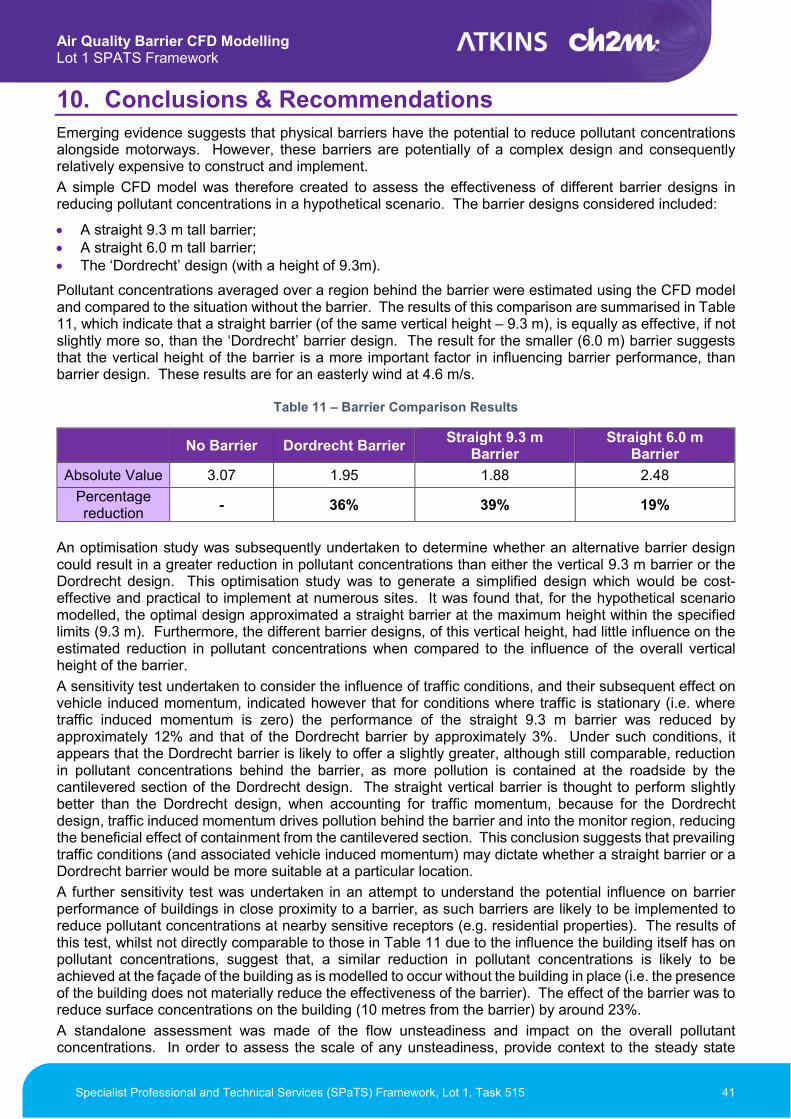
Pollutant concentrations averaged over a region behind the barrier were estimated using the CFD model and compared to the situation without the barrier. The results of this comparison are summarised in Table 11, which indicate that a straight barrier (of the same vertical height – 9.3 m), is equally as effective, if not slightly more so, than the ‘Dordrecht’ barrier design. The result for the smaller (6.0 m) barrier suggests that the vertical height of the barrier is a more important factor in influencing barrier performance, than barrier design. These results are for an easterly wind at 4.6 m/s.
Table 11 – Barrier Comparison Results
No Barrier Dordrecht Barrier Straight 9.3 m
Barrier Straight 6.0 m
Barrier
Absolute Value 3.07 1.95 1.88 2.48
Percentage reduction
- 36% 39% 19%
An optimisation study was subsequently undertaken to determine whether an alternative barrier design could result in a greater reduction in pollutant concentrations than either the vertical 9.3 m barrier or the Dordrecht design. This optimisation study was to generate a simplified design which would be cost-effective and practical to implement at numerous sites. It was found that, for the hypothetical scenario modelled, the optimal design approximated a straight barrier at the maximum height within the specified limits (9.3 m). Furthermore, the different barrier designs, of this vertical height, had little influence on the estimated reduction in pollutant concentrations when compared to the influence of the overall vertical height of the barrier.
A sensitivity test undertaken to consider the influence of traffic conditions, and their subsequent effect on vehicle induced momentum, indicated however that for conditions where traffic is stationary (i.e. where traffic induced momentum is zero) the performance of the straight 9.3 m barrier was reduced by approximately 12% and that of the Dordrecht barrier by approximately 3%. Under such conditions, it appears that the Dordrecht barrier is likely to offer a slightly greater, although still comparable, reduction in pollutant concentrations behind the barrier, as more pollution is contained at the roadside by the cantilevered section of the Dordrecht design. The straight vertical barrier is thought to perform slightly better than the Dordrecht design, when accounting for traffic momentum, because for the Dordrecht design, traffic induced momentum drives pollution behind the barrier and into the monitor region, reducing the beneficial effect of containment from the cantilevered section. This conclusion suggests that prevailing traffic conditions (and associated vehicle induced momentum) may dictate whether a straight barrier or a Dordrecht barrier would be more suitable at a particular location.
A further sensitivity test was undertaken in an attempt to understand the potential influence on barrier performance of buildings in close proximity to a barrier, as such barriers are likely to be implemented to reduce pollutant concentrations at nearby sensitive receptors (e.g. residential properties). The results of this test, whilst not directly comparable to those in Table 11 due to the influence the building itself has on pollutant concentrations, suggest that, a similar reduction in pollutant concentrations is likely to be achieved at the façade of the building as is modelled to occur without the building in place (i.e. the presence of the building does not materially reduce the effectiveness of the barrier). The effect of the barrier was to reduce surface concentrations on the building (10 metres from the barrier) by around 23%.
A standalone assessment was made of the flow unsteadiness and impact on the overall pollutant concentrations. In order to assess the scale of any unsteadiness, provide context to the steady state

Air Quality Barrier CFD Modelling Lot 1 SPATS Framework
Specialist Professional and Technical Services (SPaTS) Framework, Lot 1, Task 515 42
results and its potential effect on barrier effectiveness, a more-detailed turbulence modelling approach was used on the straight 9.3 m barrier. The DES modelling indicated relatively good matching to the steady state result. The DES modelling result may be used to indicate that the flows and concentrations downwind of a barrier are unsteady and any work to capture the performance of the barrier must highlight the limitations of the steady state method, whether it is based on field measurement or computational models.
A potential limitation of the analysis described above is that barrier performance was only evaluated under a single wind direction and wind speed. Additional analysis was therefore undertaken to confirm the findings of this study under a range of different wind directions and wind speeds for the two better performing barriers: the Dordrecht and the 9.3 m straight barrier. This has allowed for a more complete characterisation of barrier performance under different conditions. This analysis indicates that, for the wind directions resulting in the most significant pollutant concentrations in the monitoring region, both barrier designs act to reduce these concentrations. The straight barrier outperformed the Dordrecht barrier for low and medium wind speeds for the most significant wind directions, however the Dordrecht barrier typically performed better at a higher wind speed.
In order to estimate the distance from the edge of the barrier which would be required to significantly reduce pollutant concentrations, the results for all wind conditions for each barrier were combined using an equal weighting. An equal weighting has been applied because the simulations have been performed in a generic environment with no specific information on the likely wind distribution, which will be site specific. These combined results were used to estimate the distance from the edge of the barrier required for the pollutant concentration to drop by 20% compared to the ‘no barrier’ case - assumed to represent a measurable/noticeable impact. The analysis suggests that, a distance of between 30-80 m from the southern edge of either barrier would be required for a 20% reduction in pollutant concentration at both 1.5 m and 4 m elevations. The northern end of the monitoring region is protected immediately at the edge of the barrier for both elevations for the Straight barrier and at the 1.5 m elevation for the Dordrecht barrier. A distance of 20-80 m from the Dordrecht barrier edge (depending upon the horizontal distance from the barrier) is required for a reduction in pollutant concentration of 20% at the 4 m elevation.
In terms of the likely minimum distance a barrier should extend beyond the sensitive properties which the barrier is seeking to protect, this shows that (assuming an even distribution of the wind conditions considered in this study) a Straight barrier would need to extend up to 80 m upstream of sensitive receptors to achieve a 20% reduction in the pollutant contribution from the road. However, it is recommended that further assessment is undertaken using site specific, real-world distributions of wind speed and direction, to allow weighting of the available findings with regard to the orientation of the site-specific road source to the barrier and sensitive receptors. This will allow a bespoke estimate of the extent of a barrier at any locale to be made.
Summary The results of this modelling study suggest that:
the vertical height of a barrier has a greater influence on potential barrier performance than barrier design;
a straight barrier (of the same vertical height – 9.3 m) is potentially as effective as the ‘Dordrecht’ barrier design;
based on an equal weighting of the wind conditions considered in this study, an ‘overlap’ of at least 80m of barrier is needed upstream of sensitive receptors to achieve the 20% reduction, assumed to represent a measurable/noticeable impact.

Air Quality Barrier CFD Modelling Lot 1 SPATS Framework
Specialist Professional and Technical Services (SPaTS) Framework, Lot 1, Task 515 43
11. References
[1] Centre for transport and Navigation, “Dutch Air Quality Innovation Programme concluded”, January
2010.
[2] Hans van Heeswijk Architecture. 2018. “Wielwijk and Krispijn Sound Barriers.” [ONLINE] Available at:
https://www.heeswijk.nl. [Accessed 26 July 2018].
[3] GRAMM Barrier Systems. 2018. “The results are clear: SmogStop works”. [ONLINE] Available at:
http://www.smogstop.co.uk/proof. [Accessed 26 July 2018].
[4] Atkins-CH2M Joint Venture. 2018. “Task 1-515 - Air Quality Barrier Computational Fluid Dynamics
Modelling”
[5] Atkins-CH2M Joint Venture: D. Bagshaw. 2018. “Air Quality Barrier – Computational Fluid Dynamics
Modelling Task 1 - Literature Review & Assessment Approach”, SPATS Task 515 Documentation
[6] J. Frank, A. Hellsten, H. Schlunzen, B. Carissimo. 2007. “BEST PRACTICE GUIDELINE FOR THE
CFD SIMULATION OF FLOWS IN THE URBAN ENVIRONMENT”. [ONLINE] Available at:
http://theairshed.com/ [Accessed 01 August 2018].
[7] Richards, P. J. and Hoxley, R. P.: Appropriate boundary-conditions for computational wind engineering
models using the kappa epsilon turbulence model, J. Wind Eng. Ind. Aerodyn., 46-7, 1993
[8] Dept. for Business, Energy & Industrial Strategy. 2018. Average wind speed and deviations from the
long-term mean. [ONLINE] Available at: https://www.gov.uk/government/statistics/energy-trends-
section-7-weather. [Accessed 26 July 2018].
[9] US-EPA. 1981. “Guideline For Fluid Modeling Of Atmospheric Diffusion”. [ONLINE] Available at:
https://nepis.epa.gov/Exe [Accessed 26 July 2018].
[10] US-EPA. 1982. “Wake of a Block Vehicle in a Shear Free Boundary Flow – an Experimental and
Theoretical Study.” [ONLINE] Available at: https://nepis.epa.gov/Exe/. [Accessed 26 July 2018].
[11] Huang, L., Gong, S. L., Gordon, M., Liggio, J., Staebler, R., Stroud, C. A., Lu, G., Mihele, C., Brook,
J. R., and Jia, C. Q.: Aerosol–computational fluid dynamics modeling of ultrafine and black carbon
particle emission, dilution, and growth near roadways, Atmos. Chem. Phys., 14, 12631-12648,
https://doi.org/10.5194/acp-14-12631-2014, 2014.
[12] Wikipedia. 2018. Automobile Drag Coefficient. [ONLINE] Available at:
https://en.wikipedia.org/wiki/Automobile_drag_coefficient. [Accessed 26 July 2018].
[13] Warhaft, Z. (2000). Passive Scalars in Turbulent Flows. Annu. Rev. Fluid Mech. 32. 203-240. 10.1146/annurev.fluid.32.1.203.
[14] Wikipedia. 2018. Schmidt Number. [ONLINE] Available at:
https://en.wikipedia.org/wiki/Schmidt_number. [Accessed 26 July 2018].
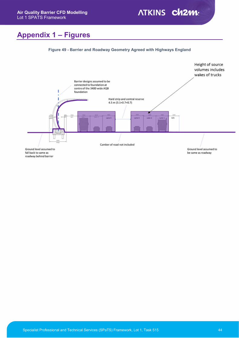
Air Quality Barrier CFD Modelling Lot 1 SPATS Framework
Specialist Professional and Technical Services (SPaTS) Framework, Lot 1, Task 515 44
Appendix 1 – Figures
Figure 49 - Barrier and Roadway Geometry Agreed with Highways England

Air Quality Barrier CFD Modelling Lot 1 SPATS Framework
Specialist Professional and Technical Services (SPaTS) Framework, Lot 1, Task 515 45
Appendix 2 – Sensitivity Test
Schmidt Number The turbulent Schmidt number (Sct) is the ratio of turbulent viscosity to turbulent mass diffusivity and can be used to characterize fluid flows where there are simultaneous momentum and mass diffusion convection processes. Sct is defined by the following equation:
��� = ��
���
where �� is the dynamic viscosity of the fluid, � is the air density and �� is the mass diffusivity.
The parameter can impact the diffusion of flow around the barrier and may have a significant effect on the levels of pollutant developed downwind. However, this study is interested in the relative difference in barrier performance and not the absolute value. If the pollutant concentration downstream of each barrier design changes by the same proportion, the choice of Schmidt number is arbitrary.
The default Schmidt number (0.9) used in most CFD simulations was applied for the previous cases. For each barrier design, a reduced and increased Schmidt number was applied, and the trends recorded. As the volume average increased or decreased by the same amount for each barrier design, the default value was retained.
Figure 50 – Schmidt Number Sensitivity