Final report

for the

‘Update of Analysis of Prospects in the Scenar 2020 Study’

Preparing for Change

Contract No. 30-CE-0200286/00-21

ECNC

LEI

ZALF

December 2009

SCENAR2020-II

Scenar 2020-II

2

Authors ECNC-European Centre for Nature Conservation

Vineta Goba Literature Review Coordinator, Project Coordinator Ben Delbaere Lawrence Jones-Walters Veronika Mikos

Landbouw-Economisch Instituut (LEI) Peter Nowicki Technical Study Coordinator Hans van Meijl Economic Analysis Coordinator Martin Banse John Helming Kristina Jansson Torbjörn Jansson Ida Terluin David Verhoog

Leibniz-Zentrum für Agrarlandschaftsforschung e.V (ZALF)

Andrea Knierim Regional SWOT Analysis Coordinator Philip Hunke Claudia Sattler Nicole Schlaefke

Editor

Glynis van Uden (ECNC) Acknowledgements We wish to express our appreciation for the thoughtful and timely guidance given by Sylvain Lhermitte, who is the officer within the European Commission following the Scenar 2020 study on behalf of the Directorate-General for Agriculture and Rural Development. We have also greatly benefited from the written and oral comments provided by the officers within several different services of the Commission. The shortcomings that may remain in this final document are the sole responsibility of the Project Team. Citation Nowicki, P., V. Goba, A. Knierim, H. van Meijl, M. Banse, B. Delbaere, J. Helming, P. Hunke, K. Jansson, T. Jansson, L. Jones-Walters, V. Mikos, C. Sattler, N. Schlaefke, I. Terluin and D. Verhoog (2009) Scenar 2020-II – Update of Analysis of Prospects in the Scenar 2020 Study – Contract No. 30–CE-0200286/00-21. European Commission, Directorate-General Agriculture and Rural Development, Brussels.

Scenar 2020-II

3

Table of contents Abbreviations ..........................................................................................................10 Preface ..................................................................................................................13 Executive summary..................................................................................................14 1. Methodological framework and defining scenarios for Scenar 2020-II ....................24

1.1. Literature review.......................................................................................24 1.2. Scenario definition.....................................................................................24

1.2.1. Summary of the Scenar 2020-II scenario proposal.....................................25 1.2.2. Further remarks on the structure of scenarios and sensitivity analyses..........28

1.3. Refining the overall analysis........................................................................29 1.3.1. Data acquisition and preparation .............................................................29 1.3.2. Economic modelling...............................................................................33 1.3.3. CAP policy implementation .....................................................................34

1.4. Regional SWOT analysis .............................................................................37 1.4.1. General methodology ............................................................................37 1.4.2. Conceptual background..........................................................................38 1.4.3. SWOT analysis in Scenar 2020-II ............................................................39

2. Literature review ...........................................................................................42

2.1. Introduction .............................................................................................42 2.2. Review of scenario studies..........................................................................42

2.2.1. Scenar 2020 – Scenario study on agriculture and the rural world .................42 2.2.2. Final report of ESPON Project 2.1.3: The territorial impact of CAP and Rural

Development Policy ...............................................................................45 2.2.3. Agriculture in the overall economy: Final report.........................................46 2.2.4. Agriculture 2013 foresight study .............................................................47 2.2.5. Agricultural commodity markets – Past developments and outlook ...............50 2.2.6. OECD-FAO Agricultural outlook 2008–2017...............................................51 2.2.7. Regions 2020: An assessment of future challenges for EU regions................54 2.2.8. Alternative futures of rural areas in the EU ...............................................55 2.2.9. Impact of EU biofuel policies on world agricultural and food markets ............56 2.2.10. Final report on the project ‘Sustainable Agriculture and Soil Conservation

(SoCo)’................................................................................................57 2.2.11. A mid-term assessment of implementing the EC Biodiversity Action Plan –

SEBI2010 Biodiversity Indicators.............................................................61 2.3. Synthesis of literature review......................................................................66

3. Refining the overall analysis – the agricultural sector ..........................................70

3.1. Introduction to the analysis of the agricultural sector......................................70 3.2. Economy-wide and global dynamics .............................................................70 3.3. Structural change – Macro trends ................................................................76 3.4. EU production and land use dynamics ..........................................................79

3.4.1. Growth in production .............................................................................79 3.4.2. Agricultural land use..............................................................................83

3.5. Commodity markets ..................................................................................84 3.5.1. Price effects .........................................................................................84 3.5.2. Quantity effects ....................................................................................85

3.6. Farm income ............................................................................................92 3.6.1. Farm income per sector (group of agricultural activities).............................92 3.6.2. Farm income at Member State level.........................................................97 3.6.3. Farm income at regional level .................................................................99

3.7. Number of farms per subsector ................................................................. 103 3.8. Employment ........................................................................................... 106

3.8.1. Agricultural employment at regional level ...............................................106 3.8.2. Changes in total regional employment....................................................110

Scenar 2020-II

4

3.9. Sensitivity analysis .................................................................................. 112 3.9.1. Sensitivity analysis for the Reference scenario.........................................112 3.9.2. Sensitivity analysis: EU-27 flat rate of first pillar premiums .......................115

4. SWOT analysis of typical rural regions’ reactions in the EU-27............................ 119

4.1. Introduction to the SWOT analysis ............................................................. 119 4.2. Socio-economic perspectives for 2020 ........................................................ 119

4.2.1. Demographic developments..................................................................120 4.2.2. Dynamics of rural economies ................................................................122 4.2.3. Typology of socio-economic perspectives................................................128

4.3. Selected structural strengths and weaknesses ............................................. 134 4.3.1. Quality of life appraisal ........................................................................134 4.3.2. Environmental preconditions.................................................................141 4.3.3. Agri-structural preconditions.................................................................160 4.3.4. Linking present preconditions with future perspectives .............................164

4.4. Agricultural performance .......................................................................... 168 4.4.1. Results of the Reference scenario ..........................................................169 4.4.2. Selected results of the Conservative and Liberalisation scenarios ...............173 4.4.3. Selected results from the agri-performance cluster combination with

environmental preconditions.................................................................174 4.4.4. Selected environmental results from alternative scenario modelling............189 4.4.5. Conclusions on agricultural performance.................................................192

4.5. Overall discussion and conclusions on the SWOT analysis .............................. 193 5. Synthesis: Preparing for change .................................................................... 196

5.1. Conclusions from the initial Scenar 2020 study ............................................ 196 5.2. Thematic axes for Scenar 2020-II synthesis ................................................ 198 5.3. Findings from Scenar 2020-II.................................................................... 200 5.4. Preparing for change ............................................................................... 204

Scenar 2020-II

5

List of tables Table 1.1: Exogenous drivers in the Scenar 2020-II scenarios. .......................................25 Table 1.2: Proposed scenarios for Scenar 2020-II. ........................................................26 Table 1.3: Coherence of the financial perspectives in the Scenar 2020-II scenarios. ..........27 Table 1.4: Tariff cuts in the Falconer proposal. .............................................................27 Table 1.5: Sensitivity analyses for the Reference scenario..............................................28 Table 1.6: Projections of regional employment growth, 2005-2020..................................31 Table 1.7: Quality of Life indicator identification. ..........................................................32 Table 1.8: Schematic overview of the models: geographical and sectoral coverage............33 Table 1.9: Treatment of Rural Development measures* in quantitative models. ................35 Table 1.10: Structure of the SWOT analysis. ................................................................40 Table 2.1: Agricultural land use (2006) ......................................................................48 Table 2.2: Arable land use (2006). .............................................................................48 Table 2.3: Main vegetable productions (2006)..............................................................48 Table 2.4: Main animal productions (2006) .................................................................48 Table 2.5: Schematic structure of Agriculture 2013 scenarios. ........................................50 Table 3.1: Composition of LEITAP categories: Crops, Livestock, Agri-food. .......................74 Table 3.2: Projected changes in producer prices for agricultural and food products in the EU-

27 under different scenarios (per cent changes). .........................................85 Table 3.3: Average real farm income per sector in the EU-27: 2020 Reference scenario

compared with 2002. ..............................................................................93 Table 3.4: Farm income per hectare or head per sector average in the EU-27: the 2020

Conservative CAP and the 2020 Liberalisation scenarios compared with the 2020 Reference scenario..................................................................................94

Table 3.5: Farm income at EU-27, EU-25, EU-15 and EU-10 levels in 2002 and in the 2020 Reference scenario (percentage difference compared with 2002). ..................97

Table 3.6: Changes in agricultural income, premiums (P1 plus P2) and sales minus purchases in 2020 Reference scenario compared with 2002 (in million euro). .................97

Table 3.7: Farm income at EU-27, EU-25, EU-15, EU-10 and Member State levels (percentage difference compared with Reference scenario). ..........................98

Table 3.8: Changes in agricultural income, premiums and sales minus purchases in Conservative CAP scenario compared with Reference scenario (million euro). ..99

Table 3.9: Number of farms per subsector in 2003 and in 2020 in different scenarios (in million farms). EU-27. ...........................................................................104

Table 3.10: Number of farms per subsector in 2003 and in 2020 in different scenarios (in million farms). EU-15. ...........................................................................105

Table 3.11: Number of farms per subsector in 2003 and in 2020 in different scenarios (in million farms). EU-12. ...........................................................................105

Table 3.12: First pillar premiums, total (first and second pillar) premiums and agricultural income in the case of a flat rate at the level of the EU-27. Percentage difference as compared with the Reference scenario. ................................................116

Table 4.1: Regional population growth rates 2004-2020 (% p.a.), according to rurality groups. ...............................................................................................121

Table 4.2: Demographic development in the EU-15 and EU-12. ....................................121 Table 4.3: Employment growth types in the EU-15 and EU-12. .....................................124 Table 4.4: Employment growth types according to the OECD rurality types. ...................125 Table 4.6: Economic types and EU old and new Member States. ...................................127 Table 4.7: Socio-economic performance groups..........................................................128 Table 4.8: Socio-economic performance in the EU-15..................................................133 Table 4.9: Socio-economic performance in the EU-12..................................................133 Table 4.10: Life satisfaction, happiness and optimism about the future in EU urban and rural

areas. .................................................................................................135 Table 4.11: Regrouping of the quality of life indicators (%). .........................................139 Table 4.12: Quality of life groups. ............................................................................139 Table 4.13: Quality of life types in the EU-15 and EU-12 and as classified according

to OECD. .............................................................................................140 Table 4.14: Areas of peat soils (ha) and share of peat soils under arable land and permanent

crops (%)............................................................................................149 Table 4.15: Land cover changes from 1990-2000 for the EU-27 as a whole. ...................150

Scenar 2020-II

6

Table 4.16: Agriculturally used soils with low organic carbon content (<2%). .................152 Table 4.17: Overview of selected environmental preconditions in EU Member States........160 Table 4.18: Characteristics of the agri-structure clusters. ............................................161 Table 4.19.: Farm-type distribution (%) in the EU-27..................................................163 Table 4.20: Farm size distribution in the EU-27. .........................................................164 Table 4.21: Scheme of selection...............................................................................165 Table 4.22a: Quality of life characteristics of the SEPT.................................................165 Table 4.22b: Regions according to OECD types per SEPT. ............................................166 Table 4.24: Selected agri-structural indicators of the SEPT...........................................167 Table 4.25: Distribution of the regions per agri-structural cluster and SEPT. ...................168 Table 4.26: Selected variables for the factor analysis as a prerequisite for the clustering of

NUTS2 regions. ....................................................................................169 Table 4.27: Extracted factors for the cluster analysis of the Reference scenario (REF). .....169 Table 4.28: Description of agri-performance clusters...................................................170 Table 4.29: Main production activities per cluster. ......................................................171 Table 4.30: Number of ‘winner’ and ‘loser’ regions per cluster in terms of income (CON and

LIB compared with REF). .......................................................................173 Table 4.31: Number of regions per cluster at NUTS2 and at HARM2 level. ......................175 Table 4.32: HARM2 regions with high shares of soils with limited available water capacity (>

15.2%) and permanent crop production (> 10%)......................................175 Table 4.33: Water abstracted for agriculture (million m³) . ..........................................177 Table 4.34: HARM2 regions challenged by high shares of sandy soils (> 34.68%) and high N-

surpluses by agricultural production (> 100 kg/ha)....................................178 Table 4.35a: FARO regions challenged by high levels of nitrate values (51-100 mg/l) per

cluster. ...............................................................................................179 Table 4.35b: FARO regions challenged by very high levels of nitrate values (101mg/l and

above) per cluster.................................................................................179 Table 4.36: HARM2 regions challenged by high shares of soils sensitive to erosion (> 20.4%)

and arable land (> 60%). ......................................................................180 Table 4.37: HARM2 regions with high shares of soils sensitive to erosion (> 20.4%) and row

crop production (> 15%). ......................................................................181 Table 4.38: HARM2 regions with high shares of Natura 2000 areas (> 19.7%) and intensive

agricultural production (> 55%)..............................................................182 Table 4.39: HARM2 regions with high shares of Natura 2000 areas (> 19.7%) and fallow land

(> 10%). ............................................................................................183 Table 4.40: Number of NUTS2 regions with high shares of High Nature Value farmland

(> 48.52%) and intensive agricultural production (> 55%).........................184 Table 4.41: NUTS2 regions with high shares of High Nature Value farmland (> 48.52%) and

unproductive land (> 10%). ...................................................................185 Table 4.42: HARM2 regions with high shares of organic soils (11.7%) and arable land

(> 50%). ............................................................................................187 Table 4.43: Country- and cluster-wise comparison of the average number of ruminants per

hectare (0.01 head/ha). ........................................................................188 Table 4.44: Percentage changes in environmental indicators; Conservative CAP and

Liberalisation scenarios as compared with 2020 Reference scenario; average EU-27. ................................................................................................189

Scenar 2020-II

7

List of figures Figure 1.1: Scheme of the SWOT tool. ........................................................................39 Figure 1.2: Scheme of SWOT analysis in Scenar 2020-II................................................41 Figure 3.1: World population, GDP, and GDP/cap annual growth rates (2007-2020)...........70 Figure 3.2: Growth of agricultural private consumption (volume) 2007-2020, annual growth

rates (%). .............................................................................................71 Figure 3.3: Growth of agricultural production (volume) 2007-2020, annual growth

rates (%). .............................................................................................72 Figure 3.4: Change in agricultural land use, 2007-2020, in per cent. ...............................72 Figure 3.5: Decomposition of the change in exports between 2007 and 2020 in agri-food

trade EU-27, Reference and Liberalisation scenario, in billion USD. ................75 Figure 3.6: Decomposition of the change in imports between 2007 and 2020 in agri-food

trade EU-27, Reference and Liberalisation scenario, in billion USD. ................75 Figure 3.7: Sectoral structure of the economy in the EU-27 in 2007 and 2020 (Gross Value

Added share), in per cent, Reference scenario.............................................76 Figure 3.8: Share of agriculture and food processing industries in the EU-15 and EU-12 in

Gross Value Added, 2007 and 2020, in per cent, Reference scenario. .............77 Figure 3.9: Share of agriculture and food processing in the economy (Gross Value Added

share), 2007 and 2020, in per cent. ..........................................................77 Figure 3.10: Development of agricultural and non-agricultural wages, EU-27, period 2007–

2020, in per cent. ...................................................................................78 Figure 3.11: Change in land price and use, EU-27, 2007–2020, in per cent. .....................79 Figure 3.12: Decomposition of growth (volume) in agri-food production, EU-27, 2007–2020,

in per cent.............................................................................................80 Figure 3.13 Decomposition of growth (volume) in livestock production, EU-27, 2007–2020, in

per cent. ...............................................................................................81 Figure 3.14: Decomposition of growth (volume) in the production of the crops (grains,

oilseeds, sugar) that can also be used for biofuels, EU-27, 2007–2020, in per cent. ....................................................................................................82

Figure 3.15: Decomposition of agricultural land-use changes, EU-27, 2007–2020, in per cent. ...............................................................................................83

Figure 3.16: Cereal production and land use under different scenarios in the EU, 2005 and 2020...............................................................................................86

Figure 3.17: Oilseed production and land use under different scenarios in the EU, 2005 and 2020...............................................................................................87

Figure 3.18: Production and consumption of beef under the different scenarios in the EU, 2005 and 2020.......................................................................................88

Figure 3.19: Production and consumption of poultry meat under the different scenarios in the EU, 2005 and 2020. ................................................................................89

Figure 3.20: Production and consumption of pork under the different scenarios in the EU, 2005 and 2020.......................................................................................90

Figure 3.21: Production and consumption of cheese under the different scenarios in the EU, 2005 and 2020.......................................................................................91

Figure 3.22: Production of and demand for biofuels under the different scenarios in the EU-27, 2005 and 2020, in Mtoe.1 ...................................................................92

Figure 3.23: Changes in premiums for suckler cows in the Conservative CAP scenario as compared with the Reference scenario. ......................................................95

Figure 3.24: Changes in income from cereals (€/ha) in the Conservative CAP scenario as compared with the Reference scenario. ......................................................96

Figure 3.25: Changes in farm income at regional level in the EU-27 in the 2020 Reference (left figure), Conservative CAP (centre figure) and Liberalisation (right figure) scenarios (percentage difference compared with 2002). .............................100

Figure 3.26: Effects of the Conservative CAP scenario on farm income per region (percentage difference compared with Reference scenario)...........................................102

Figure 3.27: Effects of the Liberalisation scenario on farm income per region (percentage difference compared with Reference scenario)...........................................103

Figure 3.28: Percentage changes in agricultural employment in 2020 Reference scenario compared with 2003. ............................................................................107

Scenar 2020-II

8

Figure 3.29: Changes in agricultural employment in the 2020 Conservative CAP scenario compared with the 2020 Reference scenario. ............................................108

Figure 3.30: Changes in agricultural employment in the 2020 Liberalisation scenario compared with the 2020 Reference scenario. ............................................109

Figure 3.31: Changes in total regional employment: 2020 Conservative CAP scenario compared with the 2020 Reference scenario. ............................................110

Figure 3.32: Changes in total regional employment: 2020 Liberalisation scenario compared with 2020 Reference scenario. ................................................................111

Figure 3.33: Change in all crops compared with the crops (grains, oilseeds, sugar) that can also be used for biofuels, 2007–2020, in per cent for EU-27. .......................113

Figure 3.34: Change in agricultural income, EU-27, 2007–2020, in per cent for primary agriculture, arable production and livestock production. .............................114

Figure 3.35: Change in land prices and use, 2007–2020, in per cent for EU-27. ..............115 Figure 3.36: Change in total (first and second pillar) premiums at the regional level in the

case of a flat rate at the level of the EU-27. Percentage difference as compared with the Reference scenario. ..................................................................117

Figure 3.37: Change in income from cereals at the regional level in the case of a flat rate at the level of the EU-27. Percentage difference as compared with the Reference scenario. .............................................................................................118

Figure 4.1: The overall SWOT analysis scheme...........................................................119 Figure 4.2: Regional demographic dynamics in 2020. ..................................................122 Figure 4.3: Employment growth types in 2020. ..........................................................124 Figure 4.4: Share of agricultural employment in 2020. ................................................126 Figure 4.5: Economic dynamics types. ......................................................................127 Figure 4.6: The SWOT scheme for the socio-economic reaction types. ...........................129 Figure 4.7: Gamma groups......................................................................................130 Figure 4.8: Beta groups. .........................................................................................131 Figure 4.9: Alpha groups.........................................................................................132 Figure 4.10: The Green Background Landscape Index, displayed in shades of green. .......137 Figure 4.11: The Green Background Landscape Index (GBLI) per FARO region................138 Figure 4.12: Distribution of the quality of life groups. ..................................................140 Figure 4.13: Share of soils with low or very low subsoil and topsoil available water

capacity (%). .......................................................................................142 Figure 4.14: Observed changes in annual precipitation 1960 to 2006.............................143 Figure 4.15: Share of sandy soils per FARO region......................................................144 Figure 4.16: Average maximum values of nitrates in groundwater per FARO region. ........145 Figure 4.17: Share of soils sensitive to erosion per FARO region (%). ............................146 Figure 4.18: Share of soils rich in soil organic matter per FARO region (%). ...................147 Figure 4.19: Share of peat soils under arable land and permanent crops (%)..................149 Figure 4.20: Land cover change (conversion from pasture, forest and wetland to arable land

or permanent crops) between 1990 and 2000 per FARO region (%). ............151 Figure 4.21: Share of agriculturally used soils with low organic carbon content (< 2%) per

FARO region (%). .................................................................................153 Figure 4.22: Share of Natura 2000 areas per FARO region (%). ....................................155 Figure 4.23: Share of High Nature Value farmland areas per NUTS2 region. ...................156 Figure 4.24: Common birds in Europe – Population index (1980 = 100) .........................157 Figure 4.25: Land cover change: % net formation 1990-2000. .....................................158 Figure 4.26: Extension of urban land by 2000 (urban sprawl and sprawl of economic sites

and infrastructures). .............................................................................158 Figure 4.27: Conversion of agricultural land cover (1990) by 2000................................159 Figure 4.28: Farm structure groups in the EU-27 (Eurostat/LEI, 2000-2005). .................162 Figure 4.29: Cluster regions in the REF scenario based on CAPRI outputs on agricultural

performance. .......................................................................................170 Figure 4.30: Boxplots for income differences in the EU-15 and EU-12 for the CON and LIB

scenarios compared with the REF scenario................................................174 Figure 4.31: Regions with high shares of permanent crops on soils with limited available soil

water..................................................................................................176 Figure 4.32: Regions with farming-generated high N-surpluses on sandy soils. ...............178 Figure 4.33: Regions with soils sensitive to erosion and high shares of arable land

production. ..........................................................................................180

Scenar 2020-II

9

Figure 4.34: Regions with soils sensitive to erosion and high shares of row crop production. ..........................................................................................181

Figure 4.35: Regions with high shares of Natura 2000 and intensive agricultural production. ..........................................................................................183

Figure 4.36: Regions with high shares of Natura 2000 and unproductive land. ................184 Figure 4.37: Regions with high shares of HNV farmland and intensive agricultural

production. ..........................................................................................185 Figure 4.38: Regions with high shares of HNV farmland and unproductive land. ..............186 Figure 4.39: Regions with high shares of organic soils and arable land...........................188 Figure 4.40: Changes in nitrogen surplus: 2020 Conservative CAP scenario compared with

2020 Reference scenario........................................................................190 Figure 4.41: Changes in nitrogen surplus: 2020 Liberalisation scenario compared with 2020

Reference scenario................................................................................191

Scenar 2020-II

10

Abbreviations ACC Accession Candidate Country BOD Biochemical Oxygen Demand CAP Common Agricultural Policy CAPRI Common Agricultural Policy Regionalised Impact modelling system CGE Computable general equilibrium CIS Commonwealth of Independent States CLC Corine Land Cover CLUE Conversion of Land Use and its Effects CMEF Common Monitoring and Evaluation Framework CPI Consumer price index DG AGRI Directorate-General for Agriculture and Rural Development DG Regio Directorate-General for Regional Policy EAFRD European Agricultural Fund for Rural Development EEA European Environment Agency EECCA Eastern Europe, Caucasus and Central Asia EFILWC European Foundation for the Improvement of Living and Working Conditions EFTA European Free Trade Association EPA Economic Partnership Agreement EPIC Erosion-Productivity Impact Calculator ESDB European Soil Database ESDP European Spatial Development Perspective ESIM European Simulation Model ESPON European Spatial Planning Observation Network ESU Economic size unit EU European Union EU-10 Ten new Member States of the European Union from May 2004 EU-12 EU-10 plus Bulgaria and Romania EU-15 Fifteen Member States of the European Union from May 2004 EU-25 Twenty-five Member States of the European Union from May 2004

Scenar 2020-II

11

EU-27 EU-25 plus Accession countries (Romania and Bulgaria) FADN Farm Accountancy Data Network (DG AGRI, European Commission) FAPRI Food and Agricultural Policy Research Institute FARO Foresight Analysis of Rural Areas of Europe (EU FP6 Specific Targeted Research

Project) FTA Free trade agreement GAEC Good agricultural and environmental condition GBLI Green Background Landscape Index GDP Gross Domestic Product GE General Equilibrium GHG Greenhouse gas GTAP Global Trade Analysis Project HC Health Check HDI Human Development Index (United Nations) HNV High Nature Value IGO Intergovernmental organisation JRC Joint Research Centre LEADER Liaisons Entre Actions de Développement de l’Economie Rurale LEITAP Extended GTAP (Global Trade Analysis Project) version implemented by LEI (Landbouw Economisch Instituut) LFA Less-Favoured Areas MENA Middle East and North Africa Mtoe Million ton oil equivalent N2K Natura 2000 NMS New Member States NMS10 New Member States that joined the EU in 2004 (Cyprus, Czech Republic,

Estonia, Hungary, Latvia, Lithuania, Malta, Poland, Slovakia and Slovenia) NUTS Nomenclature of Territorial Units for Statistics OECD Organisation for Economic Co-operation and Development P1 Pillar 1 P2 Pillar 2 PE Partial equilibrium

Scenar 2020-II

12

PEM Policy Evaluation Model PPS Purchasing power standards R&D Research and Development RDP Rural Development Policy RDR Rural Development Regulation RED Renewable Energy Directive SA Sensitivity analysis SAPARD Special Accession Programme for Agriculture and Rural Development SBL Safe biological limits SEE South-East Europe SEPT Socio-economic performance types SFP Single Farm Payment SG Steering Group SME Small and medium enterprises SMR Statutory Management Requirement SOM Soil organic matter SPS Sanitary and phytosanitary measures SWOT Strengths, Weaknesses, Opportunities and Threats analysis TRQ Tariff Rate Quota UAA Utilised Agricultural Area WTO World Trade Organisation

Scenar 2020-II

13

Preface The initial Scenar 2020 study, delivered to the Directorate-General for Agriculture and Rural Development in December 2006, has a place in a series of foresight studies intended to clarify the dominant trends in the European Union, namely as these would affect the rural economy and the agricultural sector. The first Scenar 2020 study set out to investigate the role of the agricultural sector within the rural economy, at a future horizon of 2020, within the socio-economic framework in which ‘rural’ was no longer synonymous with ‘agriculture’. The first Scenar 2020 study had as a subtitle: Understanding Change. In the two years separating the first study and the current work, many of the underlying conditions are similar, but certainly the economic crisis gives an additional perspective as to the acuteness of the dynamic of change currently at work. Today, understanding change is an insufficient attitude; rather it is necessary to be actively Preparing for Change. The rural economy depends upon rural demographic patterns, logistic infrastructure – such as transportation, communications, public services – and the natural and social constraints on land use. The specific impact of the agricultural sector depends upon agricultural technology and agricultural markets. The attributes of the urban economy – industrial production and service sector activity – increasingly permeate the rural world. The existing settlement patterns determine what is ‘rural’, in the sense that the OECD classification for the urban–rural status of territorial units depends on a double criterion of population density and the size of the urban districts within these units. The objective of the Scenar 2020-II study is to refine and add to the identification of major future trends and driving factors for European agriculture and rural regions – and the perspectives and challenges resulting from them – provided by the initial Scenar 2020 study. The methodology employed is a scenario-based macro-economic analysis that is completed by a regional ‘SWOT’ analysis of economic, social and environmental factors to identify regional patterns of development and change. As with the first study, the present study considers the challenges for agriculture and the rural areas within the European Union that are posed by demographic and socio-economic trends, globalisation, changing environmental conditions and the continuing reform of agricultural policy. The methods employed in Scenar 2020-II are based on existing economic models and other analytical methods taken from statistics, but with innovations that mean that these tools are often used at the limits of their proven capacities. There is a need for further elaboration of these tools that the reader should keep in mind. The reader is invited to address any critiques of the outcomes of the study to the project team in the perspective of improving their capacity to provide policy-related insights. Finally, to close with the same words of caution used for the initial Scenar 2020 study:

The reader is reminded that no scenario study can claim to present what will happen, but merely can portray what may happen. What is important afterwards is that these eventualities are debated, and that the necessary choices concerning the future of agriculture and the rural world are as fully informed as possible. This is the purpose of Scenar 2020.

Scenar 2020-II

14

Executive summary Objectives, drivers and scenarios Background The initial Scenar 2020 study carried out in 2006 identified and analysed a number of long-term trends concerning the demographic developments in rural regions, the dynamics of rural areas and the future of the agricultural economy including the environmental dimension for the EU, in its planned and potential future geographical shape until 2020. Two years later the exercise has been repeated. In this period the policy environment concerning the Common Agricultural Policy (CAP), the bilateral and global discussions concerning trade of agricultural commodities, and Community objectives for the natural environment (including the mitigation of climate change) have evolved considerably. A milestone has been the Health Check in 2008, designed to review and adjust the impact of the reforms enacted by the mid-term review of the CAP in 2003, notably the implementation of the new rules concerning agricultural payments in Pillar 1 and Pillar 2 of the CAP. As from 2005, the decoupling of financial support in Pillar 1 from the production of agricultural commodities has been accompanied by the introduction of a cross compliance mechanism which leads to reduction of direct payments if legal standards on environment, food safety, and animal welfare and good agricultural and environmental conditions of agricultural lands are not respected. Above this baseline, targeted payments of rural development cover a range of measures from the competitiveness of the sector to the sustainable use of natural resources and of agricultural production, and ultimately to the continued vitality of rural communities. Drivers influencing the evolution of agriculture up to 2020 As with the initial Scenar 2020, in Scenar 2020-II there are two sets of ‘drivers’ that are assumed to influence the evolution of agriculture up to 2020. The first set consists of the exogenous drivers, those that are not substantially altered by EU policy decisions within the time period of the study. These are population growth, macro-economic growth, consumer preferences, agri-technology, environmental conditions and world markets. The second set comprises the endogenous, or policy-related drivers that are expected to have a discernible effect within the Scenar 2020-II time horizon. These are EU agricultural policy, enlargement decisions and implementation, World Trade Organisation (WTO) and selected EU bilateral agreements, renewable energy policy and environmental policy. Quite obviously, this distinction between exogenous and endogenous drivers is a simplification of reality, but the purpose is to be able to have a contrast in scenario options that permits a didactic exposition of the possible consequences of policymaking. The three policy scenarios in Scenar 2020-II Three policy scenarios, indeed, are proposed within the Scenar 2020-II study. The first is a ‘Reference’ scenario, in which plausible policy decisions, based on current CAP orientations, are carried forward in the time period of the study. Particularly, this means a 20% reduction of CAP budget in real terms (constant in nominal terms), the implementation of a Single Payment System (SPS) as of 2013, full decoupling, a 30% decrease in direct payments (DP) in nominal terms and a 105% increase of the European Agricultural Fund for Rural Development (EAFRD). Trade agreements are synthetically represented, e.g. the WTO Agreement is based on the Falconer paper. The second is a ‘Conservative CAP’ scenario, which refers to a situation in which Pillar 1 payments remain higher than currently assumed, and where as a consequence – to achieve a financial balance in the assumed budget for the period – the Pillar 2 payments are commensurably less. This means a 20% reduction of CAP budget in real terms (constant in nominal terms), the continuation of the results of the Health Check (HC) after 2013, a flat rate (regional model) implemented at national level, coupling as HC, and a reduced decrease (15%) of direct payments in nominal terms, a reduced (45%) increase of EAFRD relative to the Reference scenario. Trade policies are maintained as in the Reference scenario. The third is a ‘Liberalisation’ scenario, in which all trade-related measures that impede full liberty in the export and import of agricultural products are discontinued, otherwise referred

Scenar 2020-II

15

to as the removal of trade barriers. The CAP budget is reduced by 75% in real terms (55% in nominal terms), all direct payments and market instruments are removed, and there is a 100% increase of EAFRD. Biofuel targets of 10% in 2020, as set out in the EU Renewable Energy Directive are incorporated in all three scenarios. For the sake of simplification, certain possibilities – such as the further enlargement of the EU – are not taken into account. Methodology: Macro-economic and SWOT analyses The comparison between scenarios occurs in two steps. The first step is a modelling exercise that analyses the likely outcome of each scenario using simulation models and other quantitative analyses. This is done to understand the range of potential shifts in agricultural production, income and markets which is the first purpose of this study. Where appropriate and necessary, these in-depth scenario analyses are complemented by qualitative analyses and expert judgement. The result is a description about how each scenario is expressed in spatial terms, across the EU-27. This first type of analysis is all of a macro-economic nature, but the rural world is shaped by far more elements that in particular relate to socio-cultural and biophysical conditions. In order to capture the interplay between the possible pathways for change in the economy with the possible adjustment of the other factors that compose the framework of rural life and work in the EU, a second type of analysis is required. The choice made in the two Scenar 2020 studies is to use a ‘SWOT’ analysis approach, in which a contrast is made among a series of ‘strengths’ and ‘weaknesses’ that can be associated with a group of social and environmental conditions that appear – to a varied degree – at the regional level. For this reason, the phrase ‘regional reactions’ is used to connote a response that may be expected at the regional level to specific changes in the agricultural economy at the EU level. To better understand the range of regional responses is the second purpose of Scenar 2020. Examining more than 850 regions gives an informative overview that allows a generalising aggregation of typical regions. Nevertheless, the examination of a single region's result is not the objective and is not recommended. Overview of changes in the agricultural sector within the European Union Decline in the agricultural economy The initial Scenar 2020 study demonstrated that there is a strong probability of a decline in the contribution of the agricultural sector to total income and employment within the EU. This is confirmed by the results in Scenar 2020-II. The modelling of the agricultural economy distinguishes this potential impact at different territorial levels: EU-27, national and regional, and also brings out continuing historical contrasts between the EU-15 and EU-12 groupings of Member States. For the EU as a whole, the decline in primary production is accompanied by a decline in food-processing, in spite of the fact that sourcing for the food-processing sector may occur at the world level. This trend is facilitated by liberalisation, which accentuates the relative decline in the primary production in the EU, as it is demonstrated in the Liberalisation scenario. The impacts of the decline are unevenly distributed, because the competitiveness of agricultural production and the structure of the farming industry are enormously varied across the EU. Structural changes: crop production A few highlights of the structural changes indicated by Scenar 2020-II can be presented in terms of crop production, livestock production and employment in the agricultural sector. With regard to crop production, on the one hand there is an increase of production in all scenarios, but because of yield increases (reflecting technology improvement) the amount of land devoted to crop production can be expected to decrease. This process of reduction of land use is accentuated under liberalisation, since specialisation and economies of scale would accompany shifts in market shares based on relative prices in an open market. On the other hand, there are non-market determinants in crop demand, and the obvious reference is to biofuel production that is mandated by the Renewable Energy Directive. Certain crops, which are also used for biofuel production, fare better under various future economic conditions than others; these ‘biofuel crops’ are a subset of arable crops that will have a differentiated market under liberalisation. In particular, substitution is expected to occur

Scenar 2020-II

16

through international trade that would have a greater effect upon the internal EU production requirement of those crops used for ethanol than for those used for biodiesel. Structural changes: livestock production In the case of livestock production, the impact of different market conditions is far more contrasted, and severe, than for arable production. Pork and poultry production in the EU resists the international competition in more open markets better than beef, in spite of the fact that under a Liberalisation scenario, the consumption per capita of beef relative to pork and poultry might be expected to increase because of a lower price for beef (indeed, it would drop in a liberalised trade context). The dairy market is more complex, as what distinguishes the milk market from meat sales is the possible transformation of milk into other products: butter, cheese and milk powder. Here the market penetration in a global context reflects certain competitive advantages for the EU with regard to cheese, even under a fully liberalised market. Structural changes: agricultural employment The impact of projected changes in crop and livestock production is uneven in the EU, and can be seen in the contrast between agricultural production systems of the EU-12 and EU-15. In the former case, the presence of a relatively larger amount of smaller and inefficient agricultural production units leads to a decline in income and to the shedding of agricultural employment, simply because of the incapacity to benefit from economies of scale that larger units in the EU-15 are able to achieve. The loss of agricultural employment in the EU-12 is compounded by an industrial sector also undergoing a process of restructuring. The implication is that migratory pressures can be expected from rural to urban centres within the EU-12, and from east to west in the EU as a whole. Decline in agricultural land prices If production increases through productivity gains and nevertheless less agricultural land is used, then this fact will be mirrored in a decline in prices for land, and this is what is seen in the different scenario outcomes. In the Reference and especially the Conservative CAP scenarios the decline in land prices is limited (-3.5% and -1%, respectively), whereas land prices decrease substantially in the Liberalisation scenario (-30%). When decomposing the various influences on land prices within the agricultural sector, the modelling permits an estimation of the relative importance of different aspects of policy-related influences. Reducing border measures and direct payments are the key driving factors behind the decline in land prices in the Liberalisation scenario. Mandated biofuel production strengthens land demand, and therefore has a positive repercussion on land prices. Less-Favoured Areas and Natura 2000 measures (Pillar 2) should also contribute to sustaining land prices. These influences on land prices appear to vary directly in terms of the scenario. Other effects, related to EAFRD financial support measures for agricultural enterprises regarding human and physical capital investment, basically contribute to greater productivity in EU agriculture. Environmental effects The decrease of crop and beef production in some areas could have a positive impact because, for example, there would be a decrease in nitrate use and methane emissions. But beyond a certain threshold of reduction in activity, there will be land abandonment in less competitive areas. The latter can have serious negative environmental implications as many valuable habitats and the site-specific biodiversity depend on appropriate levels of land management. The regional expression of the impact of production level changes depends on the mix of agricultural production types, as is discussed in the regional analysis part of Scenar 2020-II. Finally, as the technological attributes of agriculture are changing, reduced environmental impact through greater mastery of production methods is expected. The regional analysis showed that this was an essential development for regions with particular environmental risks. Global dynamics impacting upon agricultural commodities There is a contrast between the projected growth rate for crop and livestock production outside and within the EU for some commodities. Livestock production, for example, is stimulated in Latin America, Asia and Africa by a growth in consumption that corresponds to a per capita increase in GDP.

Scenar 2020-II

17

Agricultural land use decreases slightly in the non-EU countries of the OECD, while in developing countries the amount of agricultural land expands, especially in countries where the possibilities to expand are greatest, such as in Central and South America (in particular Brazil) and in Africa. Increased food demand at the domestic level (Africa) or from export potential (Central and South America) appears to drive the expansion in land used for agriculture. In terms of international trade, the amount of agricultural products imported into the EU is related to the degree of border protection, and this amount is set to increase under the provisions of the Falconer proposal. Under full liberalisation, exports also increase, but to a lesser extent than imports. Influence of EU policies on crop and livestock production and land use Effects of the Renewable Energy Directive and biofuel production on crop production The Renewable Energy Directive stimulates the production of the crops that are used in part for biofuel production, and this has an effect that sustains the entire agricultural economy, including positive effects on employment and land under agricultural use. In the Reference scenario, indeed, the growth of biofuel crop production within the EU is 14% up to 2020; but in the Liberalisation scenario, however, it would be only 3%. Mandated biofuel consumption in the EU is the same in both scenarios, but this does not necessarily correspond with the origin of the biofuel feedstock, as the decomposition of the factors behind the growth of biofuel crop production shows under the different scenarios. The Renewable Energy Directive would not be able to outweigh the contrary consequences of reduced border effects in the Liberalisation scenario (better competitive advantage of crops – e.g. grains, sugar – or of ethanol production outside the EU); and the reduction in Pillar 1 payments in this scenario means less support for farm income generally. Small growth in EU livestock production With regard to livestock, the foreseen increase in the consumption of meat on the global level does not translate into a major impetus for the EU livestock sector as a whole: in the Reference scenario the production of poultry increases by 15% over the study period, and pork by 7%; but beef declines by 11%. The situation depicted in the Reference scenario also takes account of the influence of border protection. The negative impact is rather limited, as in the Scenar analysis livestock is assumed to be treated as a sensitive product under the Falconer proposal. Therefore, when trade barriers are removed under the Liberalisation scenario, the projection for the growth in both poultry and pork production becomes very small over the study period, but the reduction in beef production is more than 35%. According to the decomposition analysis that has been made of all the scenarios, it can be claimed that the Renewable Energy Directive contributes to limiting the growth of all meat products, as the demand for arable crops used for biofuels would cause the feed and land for livestock to become more expensive, and the supplementary support from Pillar 2 measures does not compensate for this. Land and labour markets have an important buffer function to ease sector adjustment The impact of trade liberalisation and reducing domestic support is in general moderate; even with liberalisation agriculture will still be an important sector in Europe. The land and (to a lesser extent) the segmented labour markets play a key role in keeping production levels up as they absorb the negative impact of liberalisation by a decline in land prices and a lower growth rate of agricultural wages. These two factors contribute to keeping European agriculture competitive, along with the expected increase in productivity. Reduced agricultural land use The overall influence of liberalisation on EU-27 agricultural land use is perceptibly negative, in spite of the strong demand for arable crop land provided by the Renewable Energy Directive. A sensitivity analysis shows that the growth of biofuel crop production under the Reference scenario would even be 25% less if 2nd generation biofuels were to meet about another 25% of the mandated biofuel production requirements. Even if the economic situation within the EU is marked by growth over the long term, productivity gains in the agricultural sector diminish the land required for crops; and with the fall in beef

Scenar 2020-II

18

consumption, even the needs for grasslands for extensive pasture are progressively reduced and so is the utilised area. Finally, the removal of Pillar 1 payments under the Liberalisation scenario would also translate into reduced agricultural land use, as an important source of revenue for farming is removed. Reducing first pillar payments leads, on the one hand, to intensification of the use of land in the core production areas to earn a decent living and, on the other hand, to land abandonment in marginal production areas, as it becomes unprofitable produce in these regions. Farm income evolution and follow-on effect on farm structure Farm income is composed of several financial streams; with regard to strictly agricultural considerations, the sources of income are returns from farm sales, direct payments (Pillar 1) and EAFRD payments (Pillar 2). Decline in income The evolution of real prices for arable crops is generally negative up to the horizon of 2020 in the Reference scenario, with the exception of soybean, rapeseed and sunflower seed. Oilseeds have a quite high demand stimulated by the Renewable Energy Directive, with an additional component of demand through the by-product for livestock feed in the form of protein-rich oilseed cake. Livestock activities under the Reference scenario generally experience a decline in total income, although Pillar 1 and Pillar 2 support has a positive effect on income. The situation with regard to cereals changes under the Liberalisation scenario, as the part of this production that is transformed to ethanol loses its market share to imported intermediary or final products. Basically, the income from all agricultural commodity production will drop by 30% (arable) to 60% (livestock) in the Liberalisation scenario when compared with the Reference scenario. Much of this loss of income in the Liberalisation scenario would not come from a decreased revenue from sales (of the order of 2-4% for arable crops, 20% for cattle activities, and 4% for other animal production), but from the removal of direct payments (Pillar 1 support). The associated loss in asset (especially land) values would also have an impact on the financial situation of farms. The exception is, of course, cattle activities, which experience a loss in sales revenue already in the Reference scenario and even more in the Liberalisation scenario; so the fact that there is little loss in regard to diminished premiums in the Liberalisation scenario (by 4%) does not change the relative magnitude of total income loss. The effect of Pillar 2 on productivity It can be expected that Pillar 2 support will increase productivity (Axis 1 payments for human and physical capital investments), stimulate extensive production (Axis 2 payments for maintaining and enhancing the natural capital) and lead to farm diversification (Axis 3 payments stimulate diversification and improve the rural infrastructure). The Pillar 2 effect can be seen in the decomposition analysis carried out for the agri-food production in the EU-27 as a whole (even if small in comparison with the influence of trade measures, but still larger than the influence of the Renewable Energy Directive). Farm income across the EU-27 decreases in the Reference scenario on average by 7% from 2002 to 2020. The level of income would be the same under the Conservative CAP scenario, but would decrease by a further 22% under the Liberalisation scenario. Historical patterns of production make a difference in regional impact even in the Reference scenario, and for instance the overall impact in the EU-15 is negative largely because of the decrease in real prices in the livestock sector. The EU-12 benefits from the important injection of Pillar 2 financial support for productivity enhancement through physical and social capital investments. Liberalisation has the same relative impact across the EU, with little distinction between EU-15 and EU-12 at country level. The regional income perspective, nevertheless, is quite varied at the subnational level, as has been depicted within Scenar 2020-II.

Scenar 2020-II

19

Changes in farm structure and farm types The impact on farm structure within the Reference scenario is reflected in the projected change in farm numbers, which shows a drop of a third from 11 million units across the EU in 2003 to 7 million in 2020. The distribution of impact is unequal, but in general the drop is of the order of 25% in the EU-15 and 40% in the EU-12. The impact on agricultural subsectors is also unequal, with a squeeze in particular projected for mixed crop and mixed livestock farm types (considered together, these already represent less than 15% of EU farms). As can be assumed from the other indications reported previously, it is the cattle-related production that is most severely affected, but – to the contrary – ‘other animal’ units are the only farm types to increase in number. The number of farms is very negatively affected by reducing direct payments. Macro trends affecting the agricultural labour force in the EU Agricultural employment in the EU is influenced by the global situation The contribution of the agricultural sector to employment in the EU is determined by macro trends, in which the share of both the agricultural and industrial sectors in the gross value added of the economy is displaced by the development of the service sector. The prospect for the agricultural sector is a worldwide phenomenon, reflecting a limited growth in food demand and an increase in productivity. On the demand side, there is a low elasticity for an increase in crop use for food when per capita income grows; there is a higher – but limited – elasticity for meat in the human diet with income growth. On the supply side, as long as technology continues to produce beneficial effects for seed quality, commodity production and storage, and the transport of primary and processed products, then the overall amount of food available will continue to increase per hectare of land used and per unit of agricultural labour employed. Wage gap between the agricultural and other sectors in the EU Within the EU the projected loss of farm employment is accompanied by a continuing wage gap between the agricultural and the other sectors of the economy. Whereas agricultural wages may increase by 20% in real terms on the horizon of 2020 in the Reference scenario, industrial workers would see their remuneration grow by nearly 30%. Although the agricultural labour force would perhaps be slightly better rewarded under the Conservative CAP scenario, there would be a significantly lower increase in remuneration under the Liberalisation scenario, at the level of only 12%, whereas the non-agricultural worker would benefit from an income increase even slightly better than in the Reference scenario. Agricultural land prices buffer negative employment impact At the same time, the decline in agricultural land prices that corresponds to a decrease in land use during the scenario period will buffer the negative agricultural employment situation. In the economic paradigm, land substitutes with capital and labour among the factors involved in agricultural production. This is particularly the case in the Liberalisation scenario, in which a drop of 30% in land price at the horizon of 2020 is accompanied by a decline in agricultural land use of only about 5%. The land that remains in agricultural production is also being used to provide agricultural employment, even if economies of scale may lower the number of workers through productivity increases. Socio-economic performance of EU-27 regions Impact of long-term trends that affect the EU socio-economic framework as a whole When considering the socio-economic development of the EU-27 regions in a larger framework than the agricultural sector, the influence of the three scenarios is hardly important for the long-term trends of demographic development and employment. Both the growth or decline of population and employment are for most regions within a range of plus or minus 1% annual rates of changes at the regional level. There are differences in the intensity of migratory movement, which Scenar 2020-II seeks to portray, as well as the underlying causes. These may be associated with employment possibilities as well as the relative quality of life. What is most important as a conclusion is that there is no evidence that the EU-27 regions with a higher than average agricultural employment are structurally unsuited for ‘positive’ development perspectives, in both an economic and a social sense.

Scenar 2020-II

20

The dynamics of regional economies in the EU Looking in more detail to the dynamics of regional economies within the EU, the different types of growth potential are found within each of the Member States, and two-thirds of the regions have a slightly positive potential as opposed to being negative or very positive. The slightly positive ‘regional reaction’ to the economic conditions that are projected in the Reference scenario is evenly distributed across ‘most rural’, ‘intermediate rural’ and ‘most urban’ regional types.1 In terms of the employment situation, this can be considered as negative in a sixth of the regions. Herein, the ‘most urban’ category is the least associated with a negative rate of change. In terms of the very positive employment situation, it is the ‘most rural’ type that is least associated with a positive rate of change. So there seems to be a very minor distinction between the capacities of very rural regions to benefit from employment possibilities when compared with regions that are less marked by extreme rurality characteristics. When considering specifically the degree of agricultural employment in the description of the economic dynamics within a region, there are distinct patterns of agricultural employment levels. These are greater in the south-eastern and the south-western regions. There is also a combination of a high level of agricultural employment and of economic growth that is characteristic of three relatively large groups of regions, two in the south-west and one in the north-west. Further regional groupings made in Scenar 2020-II make it possible to identify regions in which the regional development potential has distinct characteristics as a combined expression of the agricultural sector, the service sector and population growth. Only a few regions – more to the east and the north of the EU – seem to be generally weak in the Scenar 2020 time horizon. A great number, distributed across the EU, have a moderate development potential; and regions with a positive development potential are spread out from the centre to the south-western and north-western parts of the EU. Small changes overall, but a difference between the EU-12 and EU-15 The general picture of the EU-27 regional socio-economic ‘reactions’ in 2020 is that of fairly small changes. The analysis shows, however, that although the different types of regional ‘reactions’ are represented throughout the EU-27, there is a certain division between the EU-12 and the EU-15, with the more positive ‘reactions’ occurring in the latter. Overall, the potential of the emerging ‘strong’ EU-12 regions, as well as of those within the southern EU-15 regions, for development in the service sector would seem to be a means for enhancing the quality of life, as agriculture will provide limited stimulus for employment or for discouraging out-migration. Quality of life within EU regions Variables used to index quality of life The indexation of quality of life requires the use of variables that can serve as proxies for a number of attributes that are subjective in nature. For the purposes of Scenar 2020-II, three variables are used: GDP per capita, regional share of the service sector in terms of GVA, and a Green Background Landscape Index.2 The results of the combination of these three variables show that in 25% of the regions the quality of life can be considered as low and in 75% as neutral; an insignificant number of 20 regions (out of 857) can be considered as having a high quality of life. Results from other studies Other studies making an analysis of quality of life including subjective valuation do so at far more aggregated levels. However, what is revealing is that there is very little distinction in urban or rural perspectives. Also, most sampling exercises give a similar level of rating: in one study, 70% of the persons surveyed are satisfied with their life; in another study, 75% express happiness with their situation; in a third study, about 65% are optimistic about the future.

1 The degree of rurality distinction is based on the OECD typology. 2 The Green Background Landscape Index is derived from a selection of aggregated Corine Land Cover classes, taken as a representation of landscape characteristics favourable to nature.

Scenar 2020-II

21

Scenar conclusions on quality of life Further proxies could be used, of course, for more precise investigations: access to health services and level of education are frequently suggested indicators. Unfortunately, the data available for the EU-27 regions are incomplete for such additional indicators, and do not allow for a systematic coverage of all the EU regions. The conclusion to be drawn from the three indicators that are used in this socio-economic regional analysis is that quality of life is rather homogeneous in the European Union, with only a relatively small portion of the population living in an area that is less favourable than the average. The quality of life analysis has been extended by integrating the three variables within a more extensive socio-economic framework that is an outcome of the regional analysis. The potential future socio-economic performance is contrasted with the current strengths and weaknesses of quality of life. Conclusions are drawn whether the present and future conditions are independent or interdependent at the regional level, and six types of ‘regional reactions’ are depicted. Although the analysis reveals a similar configuration between the groups of regions with a low quality of life situation at the present time and those with low socio-economic reactions in 2020, there is no conceptual basis to consider this as a cause-effect relationship. Again, ‘most rural’ regions are represented in all types of regions’ groups, but are dominant in the weaker ones. Agriculture in relation to environmental conditions within the EU Indicators used in Scenar 2020-II Capturing the state of the natural environment across the EU at a disaggregated regional level has proven to be complex, in particular because of a lack of standardised data and their recording within extended time series. A number of indicators have been examined or constructed for the purposes of the regional analysis performed within Scenar 2020-II. These are intended to provide information for interpreting water and soil conditions, for knowing about soil-related greenhouse gas (GHG) emission, and for understanding the state of biodiversity. The indicators are used to place the modelling results concerning regional agricultural land uses into the regional environmental context to help to determine the (potential) interaction in terms of possible vulnerabilities and risks. The regional analysis examines different types of risk areas in relation to the forms of agricultural production found in the regions concerned by the risk, in order to determine whether or not the farming practised is adapted to the environmental conditions, or whether the trend in agricultural land use will continue to sustain valuable ecosystems. Soils sensitive to erosion, water limitations and GHG emission An important risk identified is associated with a high proportion of soils sensitive to erosion within a region, a situation that concerns 35% of the regions across the EU, and 50% of the EU-12 regions. Regions with particularly limited available water capacities (16%) are more frequent in the southern parts of Europe, such as Bulgaria, Greece, Slovenia and Spain, but Austria is also concerned. A predominance of sandy soils (concerning 20% of EU regions), which are considered here as an indicator for risk of nitrate leaching when combined with intensive agriculture, is characteristic of regions in the northern EU, specifically Denmark, Finland, Germany and Poland, but also Portugal. Many northern EU regions are likely to have high shares of soils rich in soil organic matter, and may have possibilities to contribute to the reduction of GHG emission by applying appropriate land-use practices. In contrast, many regions in western, southern and south-eastern Europe have soils with a relatively low content in organic matter, which could function as potential GHG sinks if appropriate land-use measures are undertaken. Indicators of opportunity for biodiversity Two indicators of strength with regard to biodiversity are the presence of a relatively high share of Natura 2000 sites (in 37% of EU regions, and in over 50% of the EU-12 regions) and the quality of High Nature Value attributed to EU farmland. Natura 2000 land area is quite important in Bulgaria, Hungary, Slovenia and Spain. Approximately 20% of all EU regions (at NUTS2) show a high (> 48%) or very high (>71%) share of HNV farmland, on the basis of current estimates; and a few countries have a particularly high number of regions in this category, such as Austria, Greece, Portugal and Spain. In terms of potential

Scenar 2020-II

22

conflicts between changing agricultural practices (intensification, land abandonment) and biodiversity preservation (Natura 2000), the management plans that EU Member States have to put in place for each site should ensure compatible use of the land through farming, as the Natura 2000 network is an EU policy instrument for biodiversity protection. High Nature Value farming on the other hand is found on much larger areas than designated in the Natura 2000 network, covering about one-third of farmed areas in the EU, mainly in marginal areas. Risk associated with land abandonment The role of farming to maintain landscape quality and biodiversity (associated with both Natura 2000 and HNV areas) underlines the potential risk associated with land abandonment, which is apparent to different degrees in the three scenarios elaborated in the macro-economic part of Scenar 2020-II. This possibility is put into perspective by the type of subsequent regional analysis performed, and within Scenar 2020-II an attempt has been made to identify the regions particularly characterised by those types of land use that might indicate an ongoing process of land abandonment. To do this, the future shares of different farming types projected on the horizon of 2020 have been clustered to give a broad overview of agricultural performance (but only for the Reference scenario). The conditions representing a risk of land abandonment are found in a third of the EU regions. Most of the regions in this cluster are located in France, Greece, Italy, Portugal and Spain in the western and southern EU; in Bulgaria, Hungary, Poland and Romania in the eastern EU; and in Finland and Sweden in the northern EU. The reduction in agricultural utilised land projected in the macro-economic analysis with regard to the Liberalisation scenario, however, indicates the heightened risk of more widespread land abandonment within the EU as the agricultural economy becomes more liberalised. In any case in the Liberalisation scenario the Good Agricultural and Environmental Conditions (GAEC) do not apply anymore due to the cessation of direct payments in the absence of Pillar 1. Farmers will still have to fulfil requirements of the environmental legislation, without further consideration of good agricultural practices that are present in the GAEC and not in the existing legislation. In the less competitive regions, in particular, structural land abandonment would be accompanied by environmental decline. As a secondary effect of such structural change, targeted Pillar 2 measures aiming to enhance the environment would not find addressees and, therefore, could no longer contribute to sustaining extensive farming practices and thus securing the ecological values and benefits which these provide. Preparing for change

The first Scenar 2020 study had as a subtitle: Understanding Change. In the two years separating the first study and the current work, many of the underlying conditions are similar, but certainly the economic crisis gives an additional perspective as to the acuteness of the dynamic of change currently at work. Today, understanding change is an insufficient attitude; rather, it is necessary to be actively Preparing for Change. This attitude is already witnessed in the CAP reforms carried out at the European level. This current Scenar 2020 ‘update’ study tests three scenarios of the possible evolution of EU agricultural policy linked to the international market framework. Like the initial study, the current update demonstrates that the differences in CAP and trade policies have more effect on agricultural income and the number of farms than on agricultural production. Land prices and, to a lesser extent, agricultural wages play a key role in absorbing the negative impact of changes in the CAP and trade policy on the agricultural sector and rural areas and contribute to mitigating the fall in production levels. The future pattern of agricultural production in the EU will generally be subject to the international trade policy situation, as well as to purely domestic policies such as the mandated biofuels incorporation into transportation fuel resources. Direct income support is very important for farm income and for the number of farms and their balanced distribution in the EU-27. With regard to the environmental risks that are related to the agricultural activities of the Reference scenario, it can be stated that, although they are manifold, none is dominating in spatial terms or with regard to a specific orientation of agricultural production. Further changes in environmental conditions, which the agricultural sector has to deal with in the

Scenar 2020-II

23

future, are the opportunities and risks related to climate change. In this study, only a few aspects have been taken into account. A scenario study demonstrates that it is possible to anticipate the type of restructuring of the agricultural sector that is ineluctable. Considering the agricultural economy at the European scale, there is increasingly a true dichotomy in agricultural systems. On the one hand, there is a trend for specialisation (in open-field arable, horticultural and livestock-rearing/dairy systems); on the other hand, there is the livestock-based system with mixed cropping for fodder system, interlaced with fallow lands tending towards retirement from agricultural use. Both systems are valid and valuable, from a social and an environmental perspective. These trends are long term and geographically identifiable. There are aspects of agricultural land use that can be encouraged by policy instruments at the EU level in order to enhance the environmental contribution of the two types of farming systems. Postscript

No scenario study can claim to present what will happen, but merely can portray what may happen. What is important afterwards is that these eventualities are debated, and that the necessary choices concerning the future of agriculture and the rural world are as fully informed as possible.

Scenar 2020-II

24

1. Methodological framework and defining scenarios for Scenar 2020-II

The methodological framework for Scenar 2020-II has four components. A literature review is intended to place the initial Scenar 2020 study in a wider context. The definition of scenarios is in turn intended to take advantage of the larger perspective provided by the literature review. Once the scenarios are established, there are two analytical tasks: the first is to update the original data-set; and the second is to run the economic simulations again after an incorporation of revised policy parameters that reflect the outcome of the Health Check review and the progress with trade negotiations (the Falconer proposal). The last part of the study is a refinement of the original regional SWOT analysis, by which to identify and locate typical regional responses to the economic, social and policy influences upon agriculture and EU rural areas.

1.1. Literature review The Scenar 2020 study is one of several prospective studies concerning agriculture and rural areas within the EU that have been undertaken in the period 2000 to present. As the analysis of the original study is to be deepened, the perspectives of the other studies are considered as possible sources of insights that contribute to the further enhancement of the original results and the conclusions drawn upon them. The studies selected for review are as follows, and the outcome is presented in Chapter 2: 1) Scenar 2020 – Scenario study on agriculture and the rural world; DG AGRI Contract No.

30-CE-0040087/00-08; Nowicki et al., 2007. 2) ESPON Project 2.1.3: The territorial impact of CAP and Rural Development Policy. Final

report; Arkleton Centre for Rural Development Research, 2004. 3) Agriculture in the overall economy. Final report; European Commission, Project No.

AGRI-2006-G4-13; Banse & Grethe, 2007. 4) Agriculture 2013 foresight study; INRA, 2008. 5) Agricultural commodity markets - Past developments and outlook; European

Commission, 2006. 6) OECD-FAO Agricultural Outlook 2008–2017; OECD & FAO, 2008. 7) Regions 2020: An assessment of future challenges for EU regions (SEC(2008) 2868

final); European Commission, 2008b. 8) Alternative futures of rural areas in the EU; Jansson & Terluin, 2009. 9) Impact of EU biofuel policies on world agricultural and food markets; Banse et al., 2008;

paper prepared for presentation at the 107th EAAE Seminar ‘Modelling of agricultural and rural development policies’, Sevilla, Spain, 29 January–1 February 2008.

10) Final report on the project ‘Sustainable Agriculture and Soil Conservation (SoCo)' (Administrative arrangement AGRI20070336); European Commission, 2009b.

11) A mid-term assessment of implementing the EC Biodiversity Action Plan – SEBI2010 Biodiversity Indicators (COM(2008) 864 final); two volumes; European Commission, 2008c.

1.2. Scenario definition As with the initial Scenar 2020 study, an assumption that has guided the preparation of the Scenar 2020-II study is that there are two levels of drivers that influence scenario building. The first level is a set of exogenous drivers; these are drivers that are not directly influenced by policies, or at least not in the Scenar time horizon (that is, up to 2020). As presented in Table 1.1, they are population growth, macro-economic growth, consumer preferences, agri-technology and world markets.3 A particular interest of Scenar 2020-II is the influence of 3 World markets are partly endogenous in this study as we use a global economy-wide model in which world markets are dependent on macro-economic and population developments, preference shifts, technological change and policy changes.

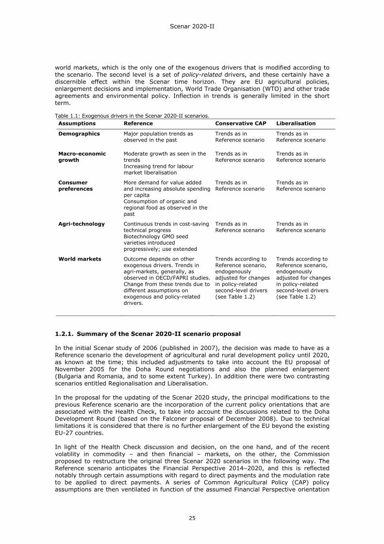
Scenar 2020-II

25

world markets, which is the only one of the exogenous drivers that is modified according to the scenario. The second level is a set of policy-related drivers, and these certainly have a discernible effect within the Scenar time horizon. They are EU agricultural policies, enlargement decisions and implementation, World Trade Organisation (WTO) and other trade agreements and environmental policy. Inflection in trends is generally limited in the short term. Table 1.1: Exogenous drivers in the Scenar 2020-II scenarios. Assumptions Reference Conservative CAP Liberalisation

Demographics Major population trends as observed in the past

Trends as in Reference scenario

Trends as in Reference scenario

Macro-economic growth

Moderate growth as seen in the trends Increasing trend for labour market liberalisation

Trends as in Reference scenario

Trends as in Reference scenario

Consumer preferences

More demand for value added and increasing absolute spending per capita Consumption of organic and regional food as observed in the past

Trends as in Reference scenario

Trends as in Reference scenario

Agri-technology Continuous trends in cost-saving technical progress Biotechnology GMO seed varieties introduced progressively; use extended

Trends as in Reference scenario

Trends as in Reference scenario

World markets Outcome depends on other exogenous drivers. Trends in agri-markets, generally, as observed in OECD/FAPRI studies. Change from these trends due to different assumptions on exogenous and policy-related drivers.

Trends according to Reference scenario, endogenously adjusted for changes in policy-related second-level drivers (see Table 1.2)

Trends according to Reference scenario, endogenously adjusted for changes in policy-related second-level drivers (see Table 1.2)

1.2.1. Summary of the Scenar 2020-II scenario proposal In the initial Scenar study of 2006 (published in 2007), the decision was made to have as a Reference scenario the development of agricultural and rural development policy until 2020, as known at the time; this included adjustments to take into account the EU proposal of November 2005 for the Doha Round negotiations and also the planned enlargement (Bulgaria and Romania, and to some extent Turkey). In addition there were two contrasting scenarios entitled Regionalisation and Liberalisation. In the proposal for the updating of the Scenar 2020 study, the principal modifications to the previous Reference scenario are the incorporation of the current policy orientations that are associated with the Health Check, to take into account the discussions related to the Doha Development Round (based on the Falconer proposal of December 2008). Due to technical limitations it is considered that there is no further enlargement of the EU beyond the existing EU-27 countries. In light of the Health Check discussion and decision, on the one hand, and of the recent volatility in commodity – and then financial – markets, on the other, the Commission proposed to restructure the original three Scenar 2020 scenarios in the following way. The Reference scenario anticipates the Financial Perspective 2014–2020, and this is reflected notably through certain assumptions with regard to direct payments and the modulation rate to be applied to direct payments. A series of Common Agricultural Policy (CAP) policy assumptions are then ventilated in function of the assumed Financial Perspective orientation

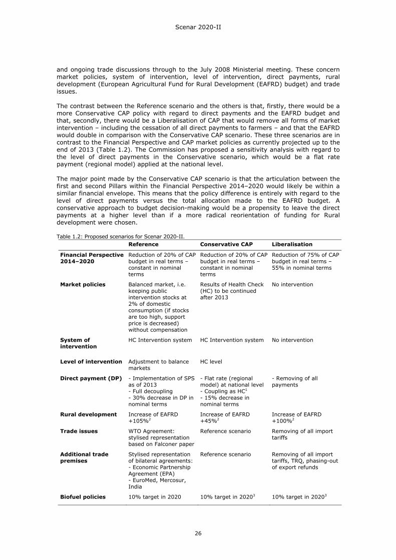
Scenar 2020-II

26

and ongoing trade discussions through to the July 2008 Ministerial meeting. These concern market policies, system of intervention, level of intervention, direct payments, rural development (European Agricultural Fund for Rural Development (EAFRD) budget) and trade issues. The contrast between the Reference scenario and the others is that, firstly, there would be a more Conservative CAP policy with regard to direct payments and the EAFRD budget and that, secondly, there would be a Liberalisation of CAP that would remove all forms of market intervention – including the cessation of all direct payments to farmers – and that the EAFRD would double in comparison with the Conservative CAP scenario. These three scenarios are in contrast to the Financial Perspective and CAP market policies as currently projected up to the end of 2013 (Table 1.2). The Commission has proposed a sensitivity analysis with regard to the level of direct payments in the Conservative scenario, which would be a flat rate payment (regional model) applied at the national level. The major point made by the Conservative CAP scenario is that the articulation between the first and second Pillars within the Financial Perspective 2014–2020 would likely be within a similar financial envelope. This means that the policy difference is entirely with regard to the level of direct payments versus the total allocation made to the EAFRD budget. A conservative approach to budget decision-making would be a propensity to leave the direct payments at a higher level than if a more radical reorientation of funding for Rural development were chosen. Table 1.2: Proposed scenarios for Scenar 2020-II. Reference Conservative CAP Liberalisation

Financial Perspective 2014–2020

Reduction of 20% of CAP budget in real terms – constant in nominal terms

Reduction of 20% of CAP budget in real terms – constant in nominal terms

Reduction of 75% of CAP budget in real terms – 55% in nominal terms

Market policies Balanced market, i.e. keeping public intervention stocks at 2% of domestic consumption (if stocks are too high, support price is decreased) without compensation

Results of Health Check (HC) to be continued after 2013

No intervention

System of intervention

HC Intervention system HC Intervention system No intervention

Level of intervention Adjustment to balance markets

HC level

Direct payment (DP) - Implementation of SPS as of 2013 - Full decoupling - 30% decrease in DP in nominal terms

- Flat rate (regional model) at national level - Coupling as HC1 - 15% decrease in nominal terms

- Removing of all payments

Rural development Increase of EAFRD +105%2

Increase of EAFRD +45%2

Increase of EAFRD +100%2

Trade issues WTO Agreement: stylised representation based on Falconer paper

Reference scenario Removing of all import tariffs

Additional trade premises

Stylised representation of bilateral agreements: - Economic Partnership Agreement (EPA) - EuroMed, Mercosur, India

Reference scenario Removing of all import tariffs, TRQ, phasing-out of export refunds

Biofuel policies 10% target in 2020 10% target in 20203 10% target in 20203

Scenar 2020-II

27

1. In the Conservative scenario, the details of the coupling are worked out so as to avoid a large transfer towards breeding (milk premium and suckler cow premium) and a very low hectare payment. 2. The increase of EAFRD goes together with a proportional increase of national co-financing, private funds and national top-ups. As the share of national co-financing is different for the different Member States, the total increase in rural development or Pillar 2 (P2) payments is also different per country. This should be taken into account, especially when reading the CAPRI (Common Agricultural Policy Regionalised modelling system) results at national and regional level. 3. The Commission and the project team decided that for the biofuel analysis the 10% target is mandatory without any subtarget for sourcing from 1st and 2nd generation technologies, in order to be consistent with the draft Renewable Energy Directive (the RED was adopted afterwards). It was also agreed that 2nd generation biofuels are counted twice in terms of energy provided for the purposes of meeting the target. Therefore, to be consistent with the prospects for agricultural markets, it was decided to keep the 10% target in all three scenarios, including the Liberalisation one. With the new directive, this means in energy terms 7% 1st generation and 1.5% 2nd generation biofuels in the three scenarios. Table 1.3 expresses the coherence of the financial perspectives established for these scenarios. Table 1.3: Coherence of the financial perspectives in the Scenar 2020-II scenarios. Reference Conservative CAP Liberalisation

Billions euro 2007 (constant) 2007 -20% -20% -75%

Billions euro nominal constant constant -55%

Total Agri nominal 55 55 55 25

Rural Dev nominal 12.4 26 18 25

Increase (nominal) in % 105% 45% 100%

Market support nominal 5.6 3.5 5.5 0

Direct payment nominal 37 25.9 31.45 0

With regard to trade issues, there are two separate groups of measures. The first concerns the multilateral negotiations and the second concerns the EU bilateral negotiations. There are three sets of issues covered under the multilateral negotiations: • Domestic support

o We assume that the scenarios given by the EU take into account the cuts as outlined in the Falconer proposal (otherwise scenario assumptions are not consistent).

• Market access o Banded tariff cuts are implemented at the CAPRI and LEITAP4 level of aggregation

from applied tariffs. o Tariff cuts as outlined in the Falconer proposal are summarised in Table 1.4.

Table 1.4: Tariff cuts in the Falconer proposal.

Band Cut Band Cut<20 50 30 33

20-50 57 30-80 3850-75 64 80-130 43> 75 70 >130 47AVG 54 36Years 5 8

DevGDevD

o Sensitive products are implemented only for the EU, Canada and the US.

4 LEITAP: extended GTAP (Global Trade Analysis Project) version implemented by LEI (Landbouw Economisch Instituut).

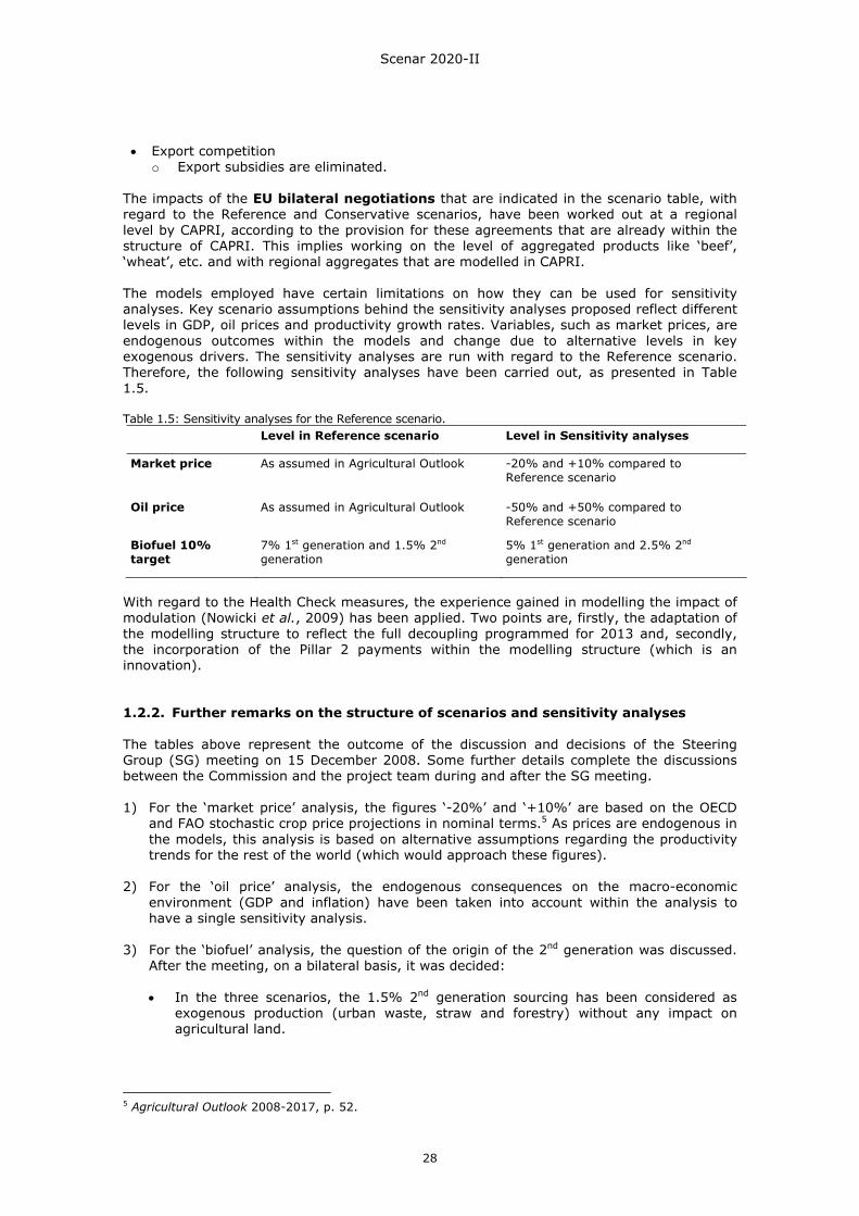
Scenar 2020-II

28

• Export competition o Export subsidies are eliminated.

The impacts of the EU bilateral negotiations that are indicated in the scenario table, with regard to the Reference and Conservative scenarios, have been worked out at a regional level by CAPRI, according to the provision for these agreements that are already within the structure of CAPRI. This implies working on the level of aggregated products like ‘beef’, ‘wheat’, etc. and with regional aggregates that are modelled in CAPRI. The models employed have certain limitations on how they can be used for sensitivity analyses. Key scenario assumptions behind the sensitivity analyses proposed reflect different levels in GDP, oil prices and productivity growth rates. Variables, such as market prices, are endogenous outcomes within the models and change due to alternative levels in key exogenous drivers. The sensitivity analyses are run with regard to the Reference scenario. Therefore, the following sensitivity analyses have been carried out, as presented in Table 1.5. Table 1.5: Sensitivity analyses for the Reference scenario. Level in Reference scenario Level in Sensitivity analyses

Market price As assumed in Agricultural Outlook -20% and +10% compared to Reference scenario

Oil price As assumed in Agricultural Outlook -50% and +50% compared to Reference scenario

Biofuel 10% target

7% 1st generation and 1.5% 2nd generation

5% 1st generation and 2.5% 2nd generation

With regard to the Health Check measures, the experience gained in modelling the impact of modulation (Nowicki et al., 2009) has been applied. Two points are, firstly, the adaptation of the modelling structure to reflect the full decoupling programmed for 2013 and, secondly, the incorporation of the Pillar 2 payments within the modelling structure (which is an innovation). 1.2.2. Further remarks on the structure of scenarios and sensitivity analyses The tables above represent the outcome of the discussion and decisions of the Steering Group (SG) meeting on 15 December 2008. Some further details complete the discussions between the Commission and the project team during and after the SG meeting. 1) For the ‘market price’ analysis, the figures ‘-20%’ and ‘+10%’ are based on the OECD

and FAO stochastic crop price projections in nominal terms.5 As prices are endogenous in the models, this analysis is based on alternative assumptions regarding the productivity trends for the rest of the world (which would approach these figures).

2) For the ‘oil price’ analysis, the endogenous consequences on the macro-economic

environment (GDP and inflation) have been taken into account within the analysis to have a single sensitivity analysis.

3) For the ‘biofuel’ analysis, the question of the origin of the 2nd generation was discussed.

After the meeting, on a bilateral basis, it was decided: • In the three scenarios, the 1.5% 2nd generation sourcing has been considered as

exogenous production (urban waste, straw and forestry) without any impact on agricultural land.

5 Agricultural Outlook 2008-2017, p. 52.

Scenar 2020-II

29

• In the sensitivity analysis, the additional 1% of 2nd generation biofuels requires agricultural land with the following conversion coefficient: for the EU an average (suitable rain-fed) land area producing 120 GJ (biofuel equivalent) per hectare for ethanol and synthetic diesel, with a range of 100–180 for marginally suitable and very suitable land.

For these three analyses, the Steering Group agreed that the sensitivity analyses would be made with LEITAP and ESIM (European Simulation Model) to have an impact assessment at European and national level (with regard to the macro-level, the agricultural sector and commodity markets). The Steering Group also agreed on a sensitivity analysis on the CAP direct payments: in the Conservative scenario, a uniform flat rate at the European level has been implemented. The sensitivity analysis on ‘climate change’ requested by the Commission was not included in the technical offer. During the discussion the interest of this analysis as well as the difficulty in its implementation in the framework of the Scenar 2020-II study were highlighted. It was decided to remove this analysis. As a result, in the Scenar 2020-II study, climate change has been addressed only in the SWOT analysis at the regional level.

1.3. Refining the overall analysis The purpose of the new Scenar 2020 study is to update the information used and the modelling results obtained in the original study to provide the input for an extended regional SWOT analysis. Thus, there are two parts to this stage of the project, which largely run in parallel. The first part involves the updating of the database and the preparation of data for use in the regional analysis. The work has thus been to verify, complete and integrate data on: • demographic development in rural areas; • economic activity in all sectors; • quality of life (social services); • environmental conditions (water resources, climate change). It should be noted that the source of this information in some cases has been generated by the economic modelling. The second part has been the preparation of the data required for the economic modelling exercise, the running of these models and the analysis of their output. The data obtained were in turn incorporated into the regional analysis. These data basically are about the projection of agricultural commodity quantities and prices, along with the evolution of the other production factors related to capital, labour and land. The regional SWOT analysis (see Section 1.4) has depended on the output of both computable general equilibrium (CGE) and partial equilibrium (PE) economic models, on the one hand, and statistical analysis for the production and grouping of primary and derived data, on the other. The statistical analysis in particular has required new data acquisition with regard to demographic development in rural areas, economic activity, quality of life and environmental conditions. 1.3.1. Data acquisition and preparation The new data have been added to the Scenar database, which contains data for measuring the development of the indicators found in the Common Monitoring and Evaluation Framework (CMEF). With regard to the regional division used, NUTS, HARM and FARO territorial units have been employed. HARM regions were used in the initial Scenar 2020 study. FARO regions have been developed to reflect labour market areas even better than HARM regions, and thus the FARO regions can be considered as appropriate territorial units for analysing regional employment growth.

Scenar 2020-II

30

1.3.1.1 Projections of regional population growth

Forecasts of population growth 2005-2050 at the national level for the EU-27 are available through the EUROPOP (2004) data-set (Eurostat, 2006). These population projections are based on assumptions about fertility, mortality and migration. By using the national population projections, Eurostat has also produced population projections at NUTS2 level for the period 2005-2030 (Eurostat, 2007). These are derived from age and sex groups within regions and internal migration between regions, and scaled with national projections. These regional projections cover 197 NUTS2 regions in 17 Member States in the EU-27 (France and the UK were omitted due to lack of regional data, and the NUTS2 level in Denmark, Luxembourg, Estonia, Cyprus, Latvia, Lithuania, Malta and Slovenia coincides with the national level). In the Scenar 2020-II study, these NUTS2 population projections form the base for the population projections for the period 2005-2020 for FARO regions, which are in most countries smaller than the NUTS2 regions. We assumed that FARO regions, which showed a slower/faster population growth per annum than that in the NUTS2 region in the period 1995-2004, also have a slower/faster population growth per annum than the projected growth rate in the NUTS2 region in the period 2005-2020. The use of population growth rates of the past for population projections could be justified as follows: Regions with a relatively low population growth in the past tend to be characterised by relatively large cohorts of older population, which may be combined with out-migration. In the period 2005-2020 the cohorts of older population have become older, so that relatively low population growth tends to stay at a low level. On the other hand, regions with a relatively high population growth in the past, are characterised by relatively large cohorts of younger population, which may be combined with in-migration. Although the cohorts of younger population have become older in the period 2005-2020, many of them are of fertility age, so population growth still tends to be at a relatively high level. 1.3.1.2 Projections of regional employment growth

In Scenar 2 projections of regional employment growth are made in order to assess whether the expected exodus of labour from the agricultural sector can be absorbed by the other sectors (industry and services) of the economy. At the regional level, employment growth is often used as an indicator for economic development. It reflects the extent to which inhabitants of the region can easily find a job or face severe shortages of employment opportunities. In the latter case, out-migration might occur.

Projections of future regional employment growth until 2020 in the EU are not available; however, there are projections of employment growth at Member State level for the periods 2004–2010, 2011–2030 and 2031–2050 (EPC, 2005). As it is outside the scope of Scenar 2 to make a very precise estimate of regional employment growth, we try to give a rough indication of the position of a region relative to the national employment growth rate. Our approach is derived from the findings from a recent comparative analysis of employment growth in OECD regions in the period 1980-1990 relative to that in the period 1990-2000 (Bollman et al., 2005). In that study, regions were classified according to their employment growth relative to the national employment growth in three groups: leading, average and lagging. On the whole, it appeared that almost 60% of all leading regions in the 1980s were still leading in the 1990s, and that also nearly 60% of the lagging regions in the 1980s were lagging in the 1990s. So quite a number of regions have a stable position in the course of time, but there are also many regions floating from period to period. Based on these findings on employment growth, we made a projection of the position of each region relative to the national employment growth in the period 2004-2020 by using its position in the period 1990-2000 and 2000-2004 (Table 1.6). The position of each region in the period 1990-2000 and 2000-2004 was calculated as follows: within each country regions are ranked according to their employment growth from high to low. The 33% regions with the highest employment growth p.a. are labelled as top 1/3 regions; the 33% regions with the lowest employment growth p.a. are labelled as bottom 1/3 and the regions in between as middle 1/3. By using the decision rules specified in the last column of Table 1.6, the region’s position in the period 2004-2020 was projected. As a final step in the regional employment projections, we assumed that all regions belonging to the middle 1/3 in the period 2004-2020 have the same employment growth rate p.a. as the national employment growth rate projected by the EU

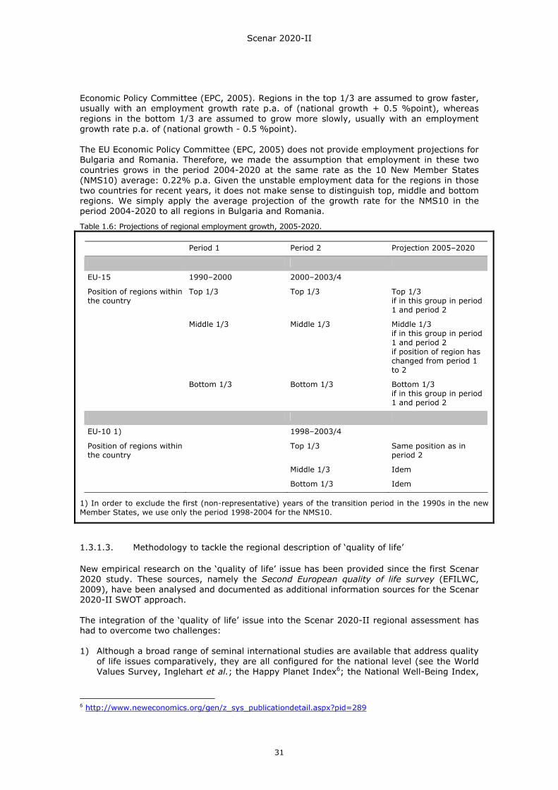
Scenar 2020-II

31

Economic Policy Committee (EPC, 2005). Regions in the top 1/3 are assumed to grow faster, usually with an employment growth rate p.a. of (national growth + 0.5 %point), whereas regions in the bottom 1/3 are assumed to grow more slowly, usually with an employment growth rate p.a. of (national growth - 0.5 %point). The EU Economic Policy Committee (EPC, 2005) does not provide employment projections for Bulgaria and Romania. Therefore, we made the assumption that employment in these two countries grows in the period 2004-2020 at the same rate as the 10 New Member States (NMS10) average: 0.22% p.a. Given the unstable employment data for the regions in those two countries for recent years, it does not make sense to distinguish top, middle and bottom regions. We simply apply the average projection of the growth rate for the NMS10 in the period 2004-2020 to all regions in Bulgaria and Romania.

Table 1.6: Projections of regional employment growth, 2005-2020.

Period 1 Period 2 Projection 2005–2020

EU-15 1990–2000 2000–2003/4

Position of regions within the country

Top 1/3 Top 1/3 Top 1/3 if in this group in period 1 and period 2

Middle 1/3 Middle 1/3 Middle 1/3 if in this group in period 1 and period 2 if position of region has changed from period 1 to 2

Bottom 1/3 Bottom 1/3 Bottom 1/3 if in this group in period 1 and period 2

EU-10 1) 1998–2003/4

Position of regions within the country

Top 1/3 Same position as in period 2

Middle 1/3 Idem

Bottom 1/3 Idem

1) In order to exclude the first (non-representative) years of the transition period in the 1990s in the new Member States, we use only the period 1998-2004 for the NMS10.

1.3.1.3. Methodology to tackle the regional description of ‘quality of life’

New empirical research on the ‘quality of life’ issue has been provided since the first Scenar 2020 study. These sources, namely the Second European quality of life survey (EFILWC, 2009), have been analysed and documented as additional information sources for the Scenar 2020-II SWOT approach. The integration of the ‘quality of life’ issue into the Scenar 2020-II regional assessment has had to overcome two challenges: 1) Although a broad range of seminal international studies are available that address quality

of life issues comparatively, they are all configured for the national level (see the World Values Survey, Inglehart et al.; the Happy Planet Index6; the National Well-Being Index,

6 http://www.neweconomics.org/gen/z_sys_publicationdetail.aspx?pid=289

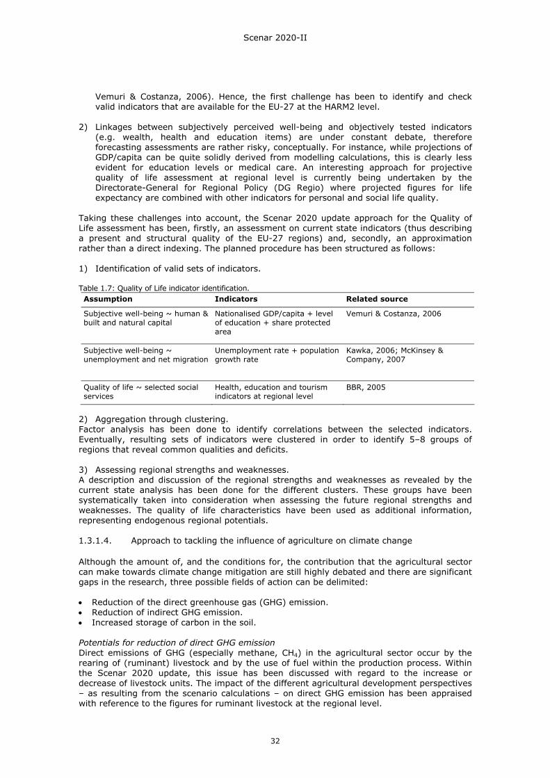
Scenar 2020-II

32

Vemuri & Costanza, 2006). Hence, the first challenge has been to identify and check valid indicators that are available for the EU-27 at the HARM2 level.

2) Linkages between subjectively perceived well-being and objectively tested indicators

(e.g. wealth, health and education items) are under constant debate, therefore forecasting assessments are rather risky, conceptually. For instance, while projections of GDP/capita can be quite solidly derived from modelling calculations, this is clearly less evident for education levels or medical care. An interesting approach for projective quality of life assessment at regional level is currently being undertaken by the Directorate-General for Regional Policy (DG Regio) where projected figures for life expectancy are combined with other indicators for personal and social life quality.

Taking these challenges into account, the Scenar 2020 update approach for the Quality of Life assessment has been, firstly, an assessment on current state indicators (thus describing a present and structural quality of the EU-27 regions) and, secondly, an approximation rather than a direct indexing. The planned procedure has been structured as follows: 1) Identification of valid sets of indicators. Table 1.7: Quality of Life indicator identification. Assumption Indicators Related source

Subjective well-being ~ human & built and natural capital

Nationalised GDP/capita + level of education + share protected area

Vemuri & Costanza, 2006

Subjective well-being ~ unemployment and net migration

Unemployment rate + population growth rate

Kawka, 2006; McKinsey & Company, 2007

Quality of life ~ selected social services

Health, education and tourism indicators at regional level

BBR, 2005

2) Aggregation through clustering. Factor analysis has been done to identify correlations between the selected indicators. Eventually, resulting sets of indicators were clustered in order to identify 5–8 groups of regions that reveal common qualities and deficits. 3) Assessing regional strengths and weaknesses. A description and discussion of the regional strengths and weaknesses as revealed by the current state analysis has been done for the different clusters. These groups have been systematically taken into consideration when assessing the future regional strengths and weaknesses. The quality of life characteristics have been used as additional information, representing endogenous regional potentials. 1.3.1.4. Approach to tackling the influence of agriculture on climate change

Although the amount of, and the conditions for, the contribution that the agricultural sector can make towards climate change mitigation are still highly debated and there are significant gaps in the research, three possible fields of action can be delimited: • Reduction of the direct greenhouse gas (GHG) emission. • Reduction of indirect GHG emission. • Increased storage of carbon in the soil. Potentials for reduction of direct GHG emission Direct emissions of GHG (especially methane, CH4) in the agricultural sector occur by the rearing of (ruminant) livestock and by the use of fuel within the production process. Within the Scenar 2020 update, this issue has been discussed with regard to the increase or decrease of livestock units. The impact of the different agricultural development perspectives – as resulting from the scenario calculations – on direct GHG emission has been appraised with reference to the figures for ruminant livestock at the regional level.

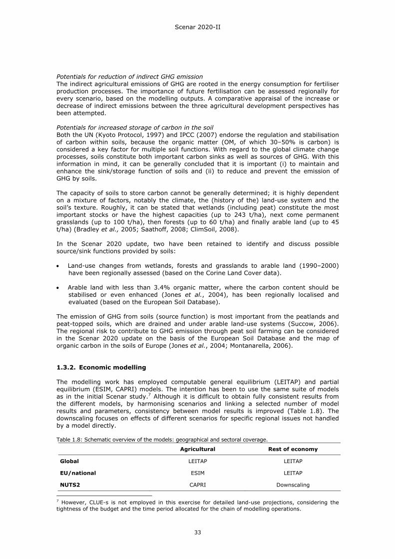
Scenar 2020-II

33

Potentials for reduction of indirect GHG emission The indirect agricultural emissions of GHG are rooted in the energy consumption for fertiliser production processes. The importance of future fertilisation can be assessed regionally for every scenario, based on the modelling outputs. A comparative appraisal of the increase or decrease of indirect emissions between the three agricultural development perspectives has been attempted. Potentials for increased storage of carbon in the soil Both the UN (Kyoto Protocol, 1997) and IPCC (2007) endorse the regulation and stabilisation of carbon within soils, because the organic matter (OM, of which 30–50% is carbon) is considered a key factor for multiple soil functions. With regard to the global climate change processes, soils constitute both important carbon sinks as well as sources of GHG. With this information in mind, it can be generally concluded that it is important (i) to maintain and enhance the sink/storage function of soils and (ii) to reduce and prevent the emission of GHG by soils. The capacity of soils to store carbon cannot be generally determined; it is highly dependent on a mixture of factors, notably the climate, the (history of the) land-use system and the soil’s texture. Roughly, it can be stated that wetlands (including peat) constitute the most important stocks or have the highest capacities (up to 243 t/ha), next come permanent grasslands (up to 100 t/ha), then forests (up to 60 t/ha) and finally arable land (up to 45 t/ha) (Bradley et al., 2005; Saathoff, 2008; ClimSoil, 2008). In the Scenar 2020 update, two have been retained to identify and discuss possible source/sink functions provided by soils: • Land-use changes from wetlands, forests and grasslands to arable land (1990–2000)

have been regionally assessed (based on the Corine Land Cover data). • Arable land with less than 3.4% organic matter, where the carbon content should be

stabilised or even enhanced (Jones et al., 2004), has been regionally localised and evaluated (based on the European Soil Database).

The emission of GHG from soils (source function) is most important from the peatlands and peat-topped soils, which are drained and under arable land-use systems (Succow, 2006). The regional risk to contribute to GHG emission through peat soil farming can be considered in the Scenar 2020 update on the basis of the European Soil Database and the map of organic carbon in the soils of Europe (Jones et al., 2004; Montanarella, 2006). 1.3.2. Economic modelling The modelling work has employed computable general equilibrium (LEITAP) and partial equilibrium (ESIM, CAPRI) models. The intention has been to use the same suite of models as in the initial Scenar study.7 Although it is difficult to obtain fully consistent results from the different models, by harmonising scenarios and linking a selected number of model results and parameters, consistency between model results is improved (Table 1.8). The downscaling focuses on effects of different scenarios for specific regional issues not handled by a model directly. Table 1.8: Schematic overview of the models: geographical and sectoral coverage.

Agricultural Rest of economy

Global LEITAP LEITAP

EU/national ESIM LEITAP

NUTS2 CAPRI Downscaling

7 However, CLUE-s is not employed in this exercise for detailed land-use projections, considering the tightness of the budget and the time period allocated for the chain of modelling operations.

Scenar 2020-II

34

To perform the analysis, a modelling framework has been constructed, consisting of three economic models (LEITAP, ESIM and CAPRI). In this modelling framework the long-term economic and environmental consequences of different scenarios are quantified and analysed, starting from 20078 up to 2020, for several regions in the world and all 27 EU countries. The LEITAP main contribution is in the WTO policies (affects all sectors, not only agriculture) and the interaction with the rest of the economy (other industries and factor markets). ESIM’s main contribution is the projection of developments in EU agricultural markets into the future. CAPRI’s main contribution is modelling changes in CAP policies and their regional impact (NUTS2 level). The downscaling is based on regional sectoral employment shares and results from CAPRI and LEITAP are combined to analyse changes in total regional employment per scenario. LEITAP is a global computable general equilibrium model that covers the whole economy including factor markets and is often used in WTO analyses (Francois et al., 2005) and CAP analyses (Meijl & Tongeren, 2002). More specifically, LEITAP is a modified version of the global general equilibrium Global Trade Analysis Project (GTAP) model. Agricultural policies are treated explicitly (e.g. production quotas, intervention prices, tariff rate quotas, (de)coupled payments). Information is used from the OECD’s Policy Evaluation Model (PEM) to improve the production structure (Hertel & Keening, 2006) and a new land allocation method, that takes into account the variation of substitutability between different types of land (Huang et al., 2004), as well as a new land supply curve are introduced (Meijl et al., 2006; Eickhout et al., 2009). Recently the model has been extended with biofuels (Banse et al., 2008) and rural development policies (Nowicki et al., 2009). The ESIM and CAPRI models are EU-27 partial equilibrium models for the agricultural sector at country and NUTS2 levels, respectively, with a strong focus on the Common Agricultural Policy. The regional disaggregation and the very detailed description of agricultural production in CAPRI enables the modelling of CAP policies in more detail compared with ESIM and LEITAP. Moreover, the CAPRI model also calculates environmental indicators and it has recently been extended by second pillar policies (Nowicki et al., 2009). ESIM contains a detailed description of the biofuel markets. Total agricultural land use is endogenous in the LEITAP model by the introduction of a land supply function based on detailed biophysical data. Total agricultural land use is given to the PE models. Yields are determined by a trend and an endogenous part dependent on prices. In ESIM yields are determined by an exogenous trend and output prices, while in LEITAP they are determined by an exogenous trend and production factor prices. Substitution effects between production factors play an important part in the LEITAP model. The elasticities of substitution are based on the GTAP database and model. From the above, it is clear that the different models are overlapping each other; but they are also complementary, with each model having its strengths and weaknesses. The approach is such that the different models analyse the same scenarios. Moreover modelling results are copied from one model to the other, e.g. productivity and efficiency changes related to human and physical capital are copied from LEITAP to CAPRI. This does, however, not guarantee that the model results are fully identical. Differences in model results occur due to differences in type of models, definitions and aggregations of variables, modelling of policies and underlying data (especially behavioural parameters and costs and revenue shares). 1.3.3. CAP policy implementation With regard to first and second pillar CAP measures, the experience gained in modelling the effect of modulation has been applied (Nowicki et al.,2009). Two points are, firstly, the adaptation of the modelling structure to reflect the full decoupling programmed for 2013 and, secondly, the incorporation of the Pillar 2 payments within the modelling structure.

8 2002 or 2003 for CAPRI, depending on the type of data being used; this is indicated in the text. 2007 for LEITAP is estimated and extrapolated data.

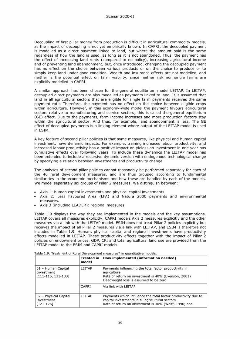
Scenar 2020-II

35

Decoupling of first pillar money from production is difficult in agricultural commodity models, as the impact of decoupling is not yet empirically known. In CAPRI, the decoupled payment is modelled as a direct payment linked to land, but where the amount paid is the same regardless of how the land is used, as long as it is not abandoned. Thus, the payment has the effect of increasing land rents (compared to no policy), increasing agricultural income and of preventing land abandonment, but, once introduced, changing the decoupled payment has no effect on the choice between various products or on the choice to produce or to simply keep land under good condition. Wealth and insurance effects are not modelled, and neither is the potential effect on farm viability, since neither risk nor single farms are explicitly modelled in CAPRI. A similar approach has been chosen for the general equilibrium model LEITAP. In LEITAP, decoupled direct payments are also modelled as payments linked to land. It is assumed that land in all agricultural sectors that are eligible for single farm payments receives the same payment rate. Therefore, the payment has no effect on the choice between eligible crops within agriculture. However, in this economy-wide model the payment favours agricultural sectors relative to manufacturing and service sectors; this is called the general equilibrium (GE) effect. Due to the payments, farm income increases and more production factors stay within the agricultural sector. And thus, for example, land abandonment is less. The GE effect of decoupled payments is a linking element where output of the LEITAP model is used in ESIM. A key feature of second pillar policies is that some measures, like physical and human capital investment, have dynamic impacts. For example, training increases labour productivity, and increased labour productivity has a positive impact on yields; an investment in one year has cumulative effects over following years. To include these dynamics the LEITAP model has been extended to include a recursive dynamic version with endogenous technological change by specifying a relation between investments and productivity change. The analyses of second pillar policies cannot reasonably be performed separately for each of the 46 rural development measures, and are thus grouped according to fundamental similarities in the economic mechanisms and how these are handled by each of the models. We model separately six groups of Pillar 2 measures. We distinguish between: • Axis 1: human capital investments and physical capital investments. • Axis 2: Less Favoured Area (LFA) and Natura 2000 payments and environmental

measures. • Axis 3 (including LEADER): regional measures. Table 1.9 displays the way they are implemented in the models and the key assumptions. LEITAP covers all measures explicitly, CAPRI models Axis 2 measures explicitly and the other measures via a link with the LEITAP model. ESIM does not treat Pillar 2 policies explicitly but receives the impact of all Pillar 2 measures via a link with LEITAP, and ESIM is therefore not included in Table 1.9. Human, physical capital and regional investments have productivity effects modelled in LEITAP. These productivity effects together with the impact of Pillar 2 policies on endowment prices, GDP, CPI and total agricultural land use are provided from the LEITAP model to the ESIM and CAPRI models. Table 1.9: Treatment of Rural Development measures* in quantitative models. Treated in

model How implemented (information needed)

LEITAP Payments influencing the total factor productivity in agriculture Rate of return on investment is 40% (Evenson, 2001) Deadweight loss is assumed to be zero

01 – Human Capital Investment [111-115, 131-133]

CAPRI Via link with LEITAP

02 – Physical Capital Investment [121-126]

LEITAP Payments which influence the total factor productivity due to capital investments in all agricultural sectors Rate of return on investment is 30% (Wolff, 1996; and

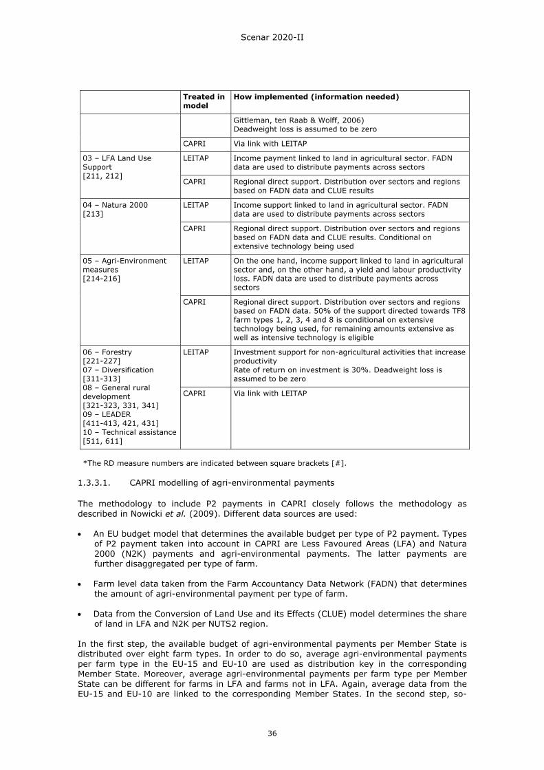
Scenar 2020-II

36

Treated in model

How implemented (information needed)

Gittleman, ten Raab & Wolff, 2006) Deadweight loss is assumed to be zero

CAPRI Via link with LEITAP

LEITAP Income payment linked to land in agricultural sector. FADN data are used to distribute payments across sectors

03 – LFA Land Use Support [211, 212]

CAPRI Regional direct support. Distribution over sectors and regions based on FADN data and CLUE results

LEITAP Income support linked to land in agricultural sector. FADN data are used to distribute payments across sectors

04 – Natura 2000 [213]

CAPRI Regional direct support. Distribution over sectors and regions based on FADN data and CLUE results. Conditional on extensive technology being used

LEITAP On the one hand, income support linked to land in agricultural sector and, on the other hand, a yield and labour productivity loss. FADN data are used to distribute payments across sectors

05 – Agri-Environment measures [214-216]

CAPRI Regional direct support. Distribution over sectors and regions based on FADN data. 50% of the support directed towards TF8 farm types 1, 2, 3, 4 and 8 is conditional on extensive technology being used, for remaining amounts extensive as well as intensive technology is eligible

LEITAP Investment support for non-agricultural activities that increase productivity Rate of return on investment is 30%. Deadweight loss is assumed to be zero

06 – Forestry [221-227] 07 – Diversification [311-313] 08 – General rural development [321-323, 331, 341] 09 – LEADER [411-413, 421, 431] 10 – Technical assistance [511, 611]

CAPRI Via link with LEITAP

*The RD measure numbers are indicated between square brackets [#].

1.3.3.1. CAPRI modelling of agri-environmental payments

The methodology to include P2 payments in CAPRI closely follows the methodology as described in Nowicki et al. (2009). Different data sources are used: • An EU budget model that determines the available budget per type of P2 payment. Types

of P2 payment taken into account in CAPRI are Less Favoured Areas (LFA) and Natura 2000 (N2K) payments and agri-environmental payments. The latter payments are further disaggregated per type of farm.

• Farm level data taken from the Farm Accountancy Data Network (FADN) that determines

the amount of agri-environmental payment per type of farm. • Data from the Conversion of Land Use and its Effects (CLUE) model determines the share

of land in LFA and N2K per NUTS2 region. In the first step, the available budget of agri-environmental payments per Member State is distributed over eight farm types. In order to do so, average agri-environmental payments per farm type in the EU-15 and EU-10 are used as distribution key in the corresponding Member State. Moreover, average agri-environmental payments per farm type per Member State can be different for farms in LFA and farms not in LFA. Again, average data from the EU-15 and EU-10 are linked to the corresponding Member States. In the second step, so-

Scenar 2020-II

37

called ‘expected’ agri-environmental payments per activity and technology in CAPRI are obtained by linking agri-environmental payments per farm type from FADN to activities and technologies per activity in CAPRI. Further relative differences in agri-environmental payments per activity per region are obtained by taking into account the share of the activity in LFA per NUTS2 region. In the third step, the exact or real agri-environmental payment per activity, technology and region in CAPRI is determined by comparing the available budget for agri-environmental payment at Member State level to the sum over the regions of the number of activities and ‘expected’ agri-environmental payment per region. The exact agri-environmental payment per activity and technology differs from the expected one, but relative differences between activities and regions are maintained.

1.4. Regional SWOT analysis 1.4.1. General methodology The SWOT analysis of the EU–27 regions was done on the basis of a broad set of multivariate statistical procedures. Hereby, the combination of methods followed the logic of reasoning when examining and appraising single and combined indicators. Mainly, factor analysis and cluster analysis were applied, as briefly described below. The comparative analysis of regions was done by deliberative grouping, ranking and qualitative assessments. 1.4.1.1. Factor analysis

The objective of factor analysis is to describe the object of investigation as exactly as possible with as few factors as possible. Hence, the communalities are usually smaller than one, because the common factors do not explain the total variance s2

i and how many factors are selected must be decided on the basis of theoretical considerations. In a first step, the independency of all variables (explaining demographics, rural economics, quality of life, environment, agriculture) is examined and complex aggregated factors are tested for whether they give a sufficiently exact evaluation/assessment (Backhaus et al., 2003, p. 308). The usual preliminary checks, e.g. the examination for normal distribution with the chi-squared test of goodness of fit and the elaboration of a correlation matrix R, are executed (Backhaus et al., 2003, p. 260). A standardisation of the data matrix is recommended, because with it a facilitation of mathematical operations and interpretations can be achieved. In addition, this allows comparability of the variables with different units. The factor analysis has been run with the program SPSS. The factor extraction is performed by application of the principal component analysis. This method enables the transfer of an m-dimensional correlation matrix in a new orthogonal m-dimensional coordinate system in such a way that a maximum of the total variance lies in the direction of the first principal axis, a maximum of the residual variance lies in the direction of the second principal axis, etc. (Überla, 1971, p. 87). The principal component analysis is finalised with a succession of orthogonal coordinate axes, along which, in descending order, each time a maximum of the total variance is localised (Überla, 1971, p. 88). In addition, the commonalities must be determined. A commonality h2

j is the part of the total variance of a variable which is explained by the common factors (Backhaus et al., 2003, p. 289). Afterwards a varimax rotation is carried out. Finally, the factor interpretation looks for the collective denomination for all variables loading highly on a factor. 1.4.1.2. Cluster analysis

Cluster analysis is an instrument to sort a heterogeneous sample of objects into homogeneous subsamples (Backhaus et al., 2003, S. 481). Cluster analysis follows on the explorative factor analysis. Similarity of the inspected objects is measured based on the Euclidean distance (Backhaus et al., 2003, S. 492). Clusters are constructed, testing different algorithms of fusion (partitioning and hierarchising procedures). In detail, the single-linkage and Ward procedures as well as the k-means clustering were applied. The single-linkage method (nearest-neighbour procedure) merges in the first step the objects i and j of two clusters Cg and Ch which are most similar, i.e. those objects where the cluster

Scenar 2020-II

38

distance is minimal. In the next step the distance of the formed group is determined to all remaining objects. As a distance between the new group and an object (group) R, the smallest value of the single distance from one of the group members and R is taken (Backhaus et al., 2003, p. 506). The procedure in general tends to the formation of many small and less large classes and to the isolation of outliers. Another important method is the Ward procedure, in which distance measure, distance calculation and clustering are determined in such a way that the sum of squared error values (variance criterion) is increased as little as possible over all groups. The objective of the procedure is to combine those objects (groups) which minimise the variation (variance) per group (Backhaus et al., 2003, p. 511). By starting from a squared error value sum of zero and by the stepwise association of other groups, most homogeneous clusters are formed until no single objects are left. The k-means procedure, a partitioning method, proceeds from a given grouping, which can result from the Ward procedure. During the procedure, the objects are shifted between the clusters until the sum of squared errors for each group has been minimised. The cluster analysis is complete if no improvement of the variance criterion can be achieved (Backhaus et al., 2003, p. 501). The identification and determination of the final number of clusters is done with regard to the inspected substantial questions. Nevertheless, further statistical analyses are done to determine the informational value of the clusters (F- and T-Value distribution). The processed data have come from three sources: • empirical data from Eurostat databases and other public sources (e.g. EEA); • projected data from time series analyses and projective calculations on Eurostat data and

other sources; • data-sets from the hierarchically integrated modelling approach (provided by LEI). 1.4.2. Conceptual background The conceptual background of the Scenar 2020-II SWOT analysis is rooted in (i) business management and organisational development theories on strategic management as described in the literature (Aeberhard, 1996; Dyson, 2004; Horn-Haacke, 2002; Nagel & Wimmer, 2008); (ii) a broad range of case descriptions of project or programme evaluation from both developed and developing countries (e.g. SDC, 2008; DG Regio, 2008a and 2008b); and (iii) pragmatic qualitative multicriteria aggregation and appraisal methods (Bechmann, 1978). According to Nagel & Wimmer (2008), the SWOT approach was elaborated as one of the essential concepts within the expert-oriented, strategic management school which conceived strategic organisational development as a rational, straightforward programme that can be planned and executed after meticulous fact-finding and analysis. Although this top-down management thinking has been overtaken by evolutionary and systemic approaches in theory and practice, the SWOT instrument is still being used. Moreover, by its adaptation for community development and resource management processes, it has become a useful tool even within participatory and change management concepts of international aid and development agencies (e.g. Borrini-Feyerabend et al., 2000; SDC, 2008; Horn-Haacke, 2002). At first glance, the generic SWOT tool convinces by its simplicity: four quadrants are arranged between a timeline (past–future) intersected by a value line (positive and negative) (Figure 1.1). These quadrants stand for (i) the acquired positive qualities, experiences and products of the inspected entity (‘Strengths’); (ii) the present negative items and deficiencies of the organism (‘Weaknesses’); (iii) the future options and development pathways that the entity could head for; and (iv) the risks and uncertainties that probably have to be faced (‘Threats’). Obviously, the first two past quadrants contain everything that has been accumulated in the past and that is within the agency of the inspected organisation, hence ‘internal’ factors, while the future quadrants stand for the organisation’s general environment, which is out of its direct reach.9 The accuracy of the distinction between these

9 Depending on the objectives of the analysis, the quadrants can be divided into subsections (e.g. KEK without year).

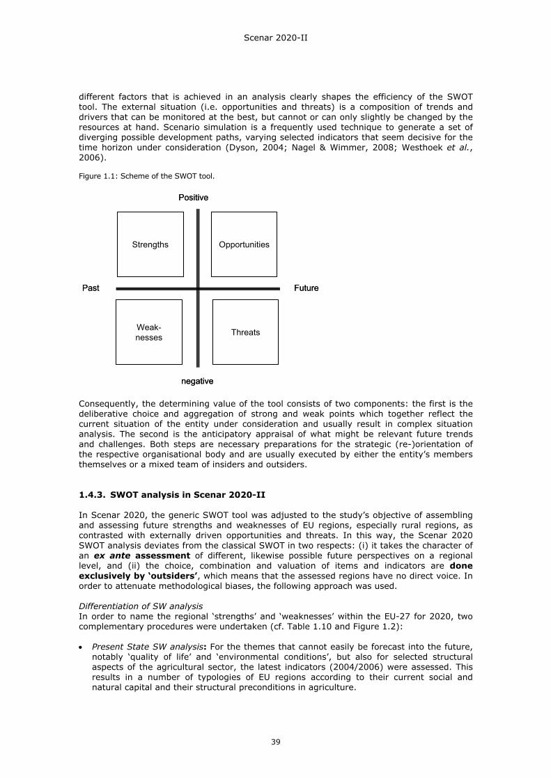
Scenar 2020-II

39

different factors that is achieved in an analysis clearly shapes the efficiency of the SWOT tool. The external situation (i.e. opportunities and threats) is a composition of trends and drivers that can be monitored at the best, but cannot or can only slightly be changed by the resources at hand. Scenario simulation is a frequently used technique to generate a set of diverging possible development paths, varying selected indicators that seem decisive for the time horizon under consideration (Dyson, 2004; Nagel & Wimmer, 2008; Westhoek et al., 2006). Figure 1.1: Scheme of the SWOT tool.

ThreatsWeak-nesses

Strengths

Positive

Opportunities

negative

Past Future

ThreatsWeak-nesses

Strengths

Positive

Opportunities

negative

Past Future

Consequently, the determining value of the tool consists of two components: the first is the deliberative choice and aggregation of strong and weak points which together reflect the current situation of the entity under consideration and usually result in complex situation analysis. The second is the anticipatory appraisal of what might be relevant future trends and challenges. Both steps are necessary preparations for the strategic (re-)orientation of the respective organisational body and are usually executed by either the entity’s members themselves or a mixed team of insiders and outsiders. 1.4.3. SWOT analysis in Scenar 2020-II In Scenar 2020, the generic SWOT tool was adjusted to the study’s objective of assembling and assessing future strengths and weaknesses of EU regions, especially rural regions, as contrasted with externally driven opportunities and threats. In this way, the Scenar 2020 SWOT analysis deviates from the classical SWOT in two respects: (i) it takes the character of an ex ante assessment of different, likewise possible future perspectives on a regional level, and (ii) the choice, combination and valuation of items and indicators are done exclusively by ‘outsiders’, which means that the assessed regions have no direct voice. In order to attenuate methodological biases, the following approach was used. Differentiation of SW analysis In order to name the regional ‘strengths’ and ‘weaknesses’ within the EU-27 for 2020, two complementary procedures were undertaken (cf. Table 1.10 and Figure 1.2): • Present State SW analysis: For the themes that cannot easily be forecast into the future,

notably ‘quality of life’ and ‘environmental conditions’, but also for selected structural aspects of the agricultural sector, the latest indicators (2004/2006) were assessed. This results in a number of typologies of EU regions according to their current social and natural capital and their structural preconditions in agriculture.

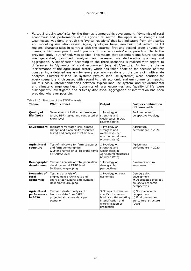
Scenar 2020-II

40

• Future State SW analysis: For the themes ‘demographic development’, ‘dynamics of rural economies’ and ‘performance of the agricultural sector’, the appraisal of strengths and weaknesses was done through the ‘typical reactions’ that key indicators from time series and modelling simulation reveal. Again, typologies have been built that reflect the EU regions’ characteristics in contrast with the external first and second order drivers. For ‘demographic development’ and ‘dynamics of rural economies’ an approach similar to the previous study, but refined, was applied. This means that essentially one future scenario was generated, described, analysed and assessed via deliberative grouping and aggregation. A specification according to the three scenarios is realised with regard to differences in ‘dynamics of rural economies’ (e.g. GVA/sector). As for the theme ‘performance of the agricultural sector’, which has fallen short so far because of time constraints, a detailed analysis for every scenario was done on the basis of multivariate analyses. Clusters of land-use systems (‘typical land-use systems’) were identified for every scenario and discussed with regard to their economic and environmental impacts. On this basis, interdependencies between ‘typical land-use system’ and ‘environmental and climate change qualities’, ‘dynamics of rural economies’ and ‘quality of life’ were subsequently investigated and critically discussed. Aggregation of information has been provided wherever possible.

Table 1.10: Structure of the SWOT analysis. Theme What is done? Output Further combination

of theme with …

Quality of life (QoL)

Several sets of indicators (analogue to UN, BBR) tested and contrasted at FARO level

1 Typology on strengths and weaknesses in QoL (current state)

Socio-economic perspective typology

Environment Indicators for water, soil, climate change and biodiversity resources tested and analysed at FARO level

1 Typology on strengths and weaknesses per environmental issue (current state)

Agricultural performance in 2020

Agricultural structure

Test of indicators for farm structures and farm demographics Cluster analysis on all relevant items at HARM2 level

1 Typology on strengths and weaknesses in Agricultural structures (current state)

Agricultural performance in 2020

Demographic development

Test and analysis of total population development at FARO level Deliberative grouping

1 Typology on demographic perspectives

Dynamics of rural economies

Dynamics of rural economies

Test and analysis of: employment growth rate and share of agricultural employment Deliberative grouping

1 Typology on rural economies

Demographic development

Aggregated typology on ‘socio-economic perspectives’

Agricultural performance in 2020

Test and cluster analysis of land-use data from CAPRI projected structural data per scenario

3 Groups of scenario-specific clusters on land use differentiating intensification and extensification of production

a) Socio-economic perspectives b) Environment and agricultural structure (2005)

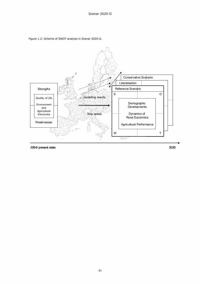
Scenar 2020-II

41

Figure 1.2: Scheme of SWOT analysis in Scenar 2020-II.

Quality of Life

Environmentand

AgriculturalStructures

2004/ present state

DemographicDevelopments

Dynamics of Rural Economics

Agricultural Performance

Reference Scenario

Liberalisation

Conservative Scenario

S O

TW

2020

modelling results

time series

Strengths

Weaknesses

Quality of Life

Environmentand

AgriculturalStructures

2004/ present state

DemographicDevelopments

Dynamics of Rural Economics

Agricultural Performance

Reference Scenario

Liberalisation

Conservative Scenario

S O

TW

2020

modelling results

time series

Strengths

Weaknesses

Scenar 2020-II

42

2. Literature review

2.1. Introduction The literature review was part of the updating and strengthening of the original work in the Scenar 2020 study. It looked at recent thinking on the future of the rural world and agricultural prospects on the horizon of 2020. The following studies were selected for review: 1) Scenar 2020 – Scenario study on agriculture and the rural world; DG AGRI Contract No.

30-CE-0040087/00-08; Nowicki et al., 2007 (abbreviated here to Scenar 2020). 2) ESPON Project 2.1.3: The territorial impact of CAP and Rural Development Policy. Final

report; Arkleton Centre for Rural Development Research, 2004 (abbreviated here to ESPON 2.1.3).

3) Agriculture in the overall economy. Final report; European Commission, Project No. AGRI-2006-G4-13; Banse & Grethe, 2007.

4) Agriculture 2013 foresight study; INRA, 2008 (abbreviated here to Agriculture 2013). 5) Agricultural commodity markets - Past developments and outlook; European

Commission, 2006 (abbreviated here to Agricultural commodity markets). 6) OECD-FAO Agricultural Outlook 2008–2017; OECD & FAO, 2008 (abbreviated here to

Agricultural Outlook 2008–2017). 7) Regions 2020: An assessment of future challenges for EU regions (SEC(2008) 2868

final); European Commission, 2008b (abbreviated here to Regions 2020). 8) Alternative futures of rural areas in the EU; Jansson & Terluin, 2009 (abbreviated here to

Alternative futures). 9) Impact of EU biofuel policies on world agricultural and food markets; Banse et al., 2008;

paper prepared for presentation at the 107th EAAE Seminar ‘Modelling of agricultural and rural development policies’, Sevilla, Spain, 29 January–1 February 2008 (abbreviated here to Impact of EU biofuel policies).

10) Final report on the project ‘Sustainable Agriculture and Soil Conservation (SoCo)' (Administrative arrangement AGRI20070336); European Commission, 2009b (abbreviated here to SoCo final report).

11) A mid-term assessment of implementing the EC Biodiversity Action Plan – SEBI2010 Biodiversity Indicators (COM(2008) 864 final); two volumes; European Commission, 2008c (abbreviated here to SEBI report).

2.2. Review of scenario studies 2.2.1. Scenar 2020 – Scenario study on agriculture and the rural world The purpose of the original Scenar 2020 study was the identification of future trends and driving forces that will be the framework for the European agricultural and rural economy on the horizon of 2020. The method used was to build a reference scenario (‘baseline’) based on an analysis of trends from 1990 to 2005, which was projected forward to 2020; the trend analysis provided a substantiated basis for determining the long-term driving forces that was reflected in the reference scenario. It was assumed that economic, agricultural and environmental policy may cause an inflection in these trends, so these were studied as a second level set of driving forces, also to be taken into account in the scenario exercise. The relative importance of various policy frameworks was understood by comparing two alternative – or ‘counterfactual’ – scenarios (‘liberalisation’ and ‘regionalisation’) with the reference scenario. The comparison between scenarios occurred in two steps: the first was a modelling exercise that analysed the likely outcome of each scenario using simulation models and other quantitative analyses. Where appropriate and necessary, these in-depth scenario analyses were complemented by qualitative analyses and expert judgement. The result was a

Scenar 2020-II

43

description of how each scenario is expressed in spatial terms, across the EU-27, and in some cases extended to the candidate countries for accession. The second step was a SWOT analysis, which was applied to each scenario in order to understand the implications in the following domains: demographic developments, dynamics of rural economies, and the future of the agricultural economy (specifically in terms of farm structures, production systems and farm population demography). Scenar 2020 aimed to take stock of the current hypotheses as to the future of agriculture markets in the expanding European Union and the likely development of the rural economic and social framework in which agriculture is practised. If it is true that rural and agricultural policies need to be distinct, then the interplay between them should take into account the long-term trends in demography, technology and markets that shape the opportunities in which these policies can provide a useful orientation to maximise the opportunities for social welfare and environmental benefits. Scenar 2020 provided a systematic review of the primary variables that rural and agricultural policies have to take into account. These are (a) the rural demographic patterns, (b) the agricultural technology, (c) the agricultural markets, and (d) the natural and social constraints on land use that are likely to exist in 2020. Social and economic factors, both conditioned by technology, have a bearing on these primary variables, and these factors are both endogenous and exogenous. Technology determines what is possible in every domain, and social (consumer) demand determines what is economically viable. Social demand – as it affects the agricultural sector – reflects not only consumer preferences in terms of food, but also environmental and health concerns, including the commitment by society as a whole to the wise use of natural resources (water, soil) and biodiversity preservation. It is these environmental and health concerns that define the natural and social constraints on land use. World markets and local production costs – including compensation measures that may offset operating charges – will inevitably both determine what is economically feasible in the EU and direct agricultural production to the geographical locations worldwide that provide sustainable livelihoods for farmers, or the greatest return on investment for agro-industrial enterprises. The general methodology of Scenar 2020 was based upon: • the establishment of an extensive database covering the period 1990–2005 to identify

drivers and corresponding trends on the global, national and regional levels; • the elaboration of indicators to interpret the data in order to formulate assumptions for

the elaboration of a baseline scenario and two policy framework scenarios up to the horizon of 2020;

• the quantification of changes in agricultural and rural economy and land use where this is possible through modelling;

• the extrapolation and downscaling of trends for some parameters where modelling is not possible;

• the interpretation of the information gained above through a SWOT analysis within the context of the scenario framework.

An assumption that guided the preparation of the scenario study is that there were two levels of drivers that would influence scenario building. The first level is a set of exogenous drivers; these are drivers that are not directly influenced by policies, or at least not in the Scenar time horizon (that is, up to 2020). They are population growth, macro-economic growth, consumer preferences, agri-technology, environmental conditions and world markets. The second level is a set of policy-related drivers, and these will certainly have a discernible effect within the Scenar time horizon. They are EU agricultural policies, enlargement decisions and implementation, World Trade Organisation (WTO) and other international agreements and environmental policy. The extensive database, which was collected for the drivers and indicators, made it possible for the modelling and trends analysis to provide the first step in the impact analysis of the three scenarios retained, identified by the terms baseline, regionalisation and liberalisation. The baseline situation was based on the continuation of the trends in exogenous drivers, and assumed the development of agricultural and rural policy according to current policy

Scenar 2020-II

44

objectives, including the successful outcome of the Doha Round negotiations. Regionalisation was a policy framework which referred to the possibility that, in the absence of a successful conclusion of the Doha Round, then not only will further bilateral and multilateral negotiations continue but also at the same time more encouragement will be given to promoting the production of commodities in the internal market. Liberalisation – also a policy framework – implied that the current context of moving towards more open markets at the international level would be strengthened. In this scenario, all forms of market and trade policies and income support – that are related to agricultural commodity production – will be abolished in the EU and the rest of the world. The main conclusions of Scenar 2020 are: • Rural areas are not stable in terms of urbanisation, changes in land use in rural areas,

marginalisation of rural areas, structural adjustment of agriculture in the EU. • Agriculture in rural areas within the EU-27 is very diverse. • The share of agricultural employment in regions is very different. In general the share is

much higher in the EU-10 (12%) than in the EU-15 (4%). There is a wide diversity in the size of holdings within the EU, but both the size and adaptability of these family units are regionally quite differentiated.

• Growth rate in world agricultural markets will slow down.

o Population growth will no longer be the major driver of agricultural demand in the future. Future world population growth will be lower. Robust economic growth is expected in almost all regions in the world. Expansion in global consumption will occur. Income growth, urbanisation and dietary diversification lead not only to additional demand but also to changes in the composition of food consumption, with a fast growing share of animal products. In developed countries food consumption growth is limited. World prices will continue to decline in real terms, due to high productivity growth and a fairly inelastic demand.

• There are several key trends in EU commodity markets up to the horizon of 2020, such

as:

o Increasing segmentation of the EU market will take place because of the growing relative importance of transportation costs, which is enhanced by further trade liberalisation and enlargement.

o Main developments in cereals: Although production will increase, area requirements will diminish because of technical productivity improvement.

o Main developments in livestock: The livestock market will undergo important restructuring, with a concentration on dairy production, poultry meat and pork meat output.

o Main developments in oilseeds: Because of the policy promotion of biofuels, independently of the external market, there will be a shift in oilseed production towards the requirements of industrial-use quality as opposed to food consumption quality.

• Structural change process in agriculture is a long-term process that continues with or

without policy changes. This structural change process includes:

o Declining share of agriculture and industry in GDP. o Declining number of people working in agriculture, both in absolute terms and as a

proportion of the total workforce. o Decrease in the number of farm units, with an increase in the average size. o Increase in diversification of farm households (e.g. part-time farming). o Enlargement has brought into the EU a wider variety of farm units. o Structural change will continue to be especially acute in the EU-12, because of the

high share of agriculture in GDP and employment and the high number of small farm units.

Scenar 2020-II

45

o The surplus agricultural labour in the EU-12 may not be easily absorbed because of a parallel decline in manufacturing employment.

o Out-migration from peripheral areas (particularly on the eastern EU frontier and in the north-west corner of the Iberian peninsula) will cause a labour deficit.

• Policy change produces differentiated impact.

o The reduction of border support (import tariffs and export subsidies) has a higher impact on agricultural production than the reduction of domestic income support.

o The process of liberalisation has a greater impact on agricultural income than on agricultural production and land use.

The most obvious effect of liberalisation will be the augmentation of the rate of decline in the number of farms in the EU; overall production will in general also decrease.

The general trends in factor markets are a decrease in agricultural labour and an increase in the capital intensity of agricultural production.

• A major uncertainty with regard to all conclusions concerning the future of biofuels is the

tightness of oil/energy markets. The impact of biofuels may be underestimated. • The role of forestry in rural areas is not given enough attention. A long-term trend in

afforestation is witnessed within several countries of the EU. • Environmental issues linked to land use concern:

o Greenhouse Gas emissions: the agricultural part has been declining and will continue to do so; with the decrease in beef and dairy herds, further methane reductions may be on the order of 5%.

o Nitrate concentrations in rivers: the greater part of trends in all countries is either downward or remaining stable, and the situation should improve as the forecast nitrogen surplus will decline in comparison with present conditions.

o Fertiliser use is predicted to decrease in the EU-15, but the possibility of new demand for biofuels might change this trend.

o Set-aside land is a prime area for expansion of biofuels feedstocks production. o The highest concentration of organic farming does not necessarily occur in areas

having the highest concentration of arable land. o There is no particular correlation between the location of Natura 2000 sites and the

particular concentration of agricultural or forestry land cover classes, but there is a significant correlation with regard to the ‘diverse natural areas’ and ‘wetlands’ classes.

2.2.2. Final report of ESPON Project 2.1.3: The territorial impact of CAP and Rural

Development Policy This report represents the final results of a research project conducted within the framework of the ESPON (European Spatial Planning Observation Network) 2000–2006 programme. The project’s main objective was to examine different policy options and their potential impacts in the future. It also aimed to provide elements for discussing adjustments in policies. The project had a territorial approach and was interested in the spatial impacts of policies, looking at the cohesion of the European territory. ESPON Project 2.1.3 commenced in August 2002 with the overall aim of deepening the understanding of territorial impacts of the EU’s Common Agricultural Policy and Rural Development Policy (CAP/RDP) through the provision of a standardised database and an analysis of territorial trends covering the EU-15 and neighbouring and accession states. In this study, therefore, empirical analysis was conducted at NUTS3 level using data from a variety of sources, some directly recorded at this level but most requiring derivation from sample and/or higher-level (e.g. NUTS2) values. The principal conclusion from this project is that in aggregate the CAP has worked against the European Spatial Development Perspective (ESDP) objective of balanced territorial

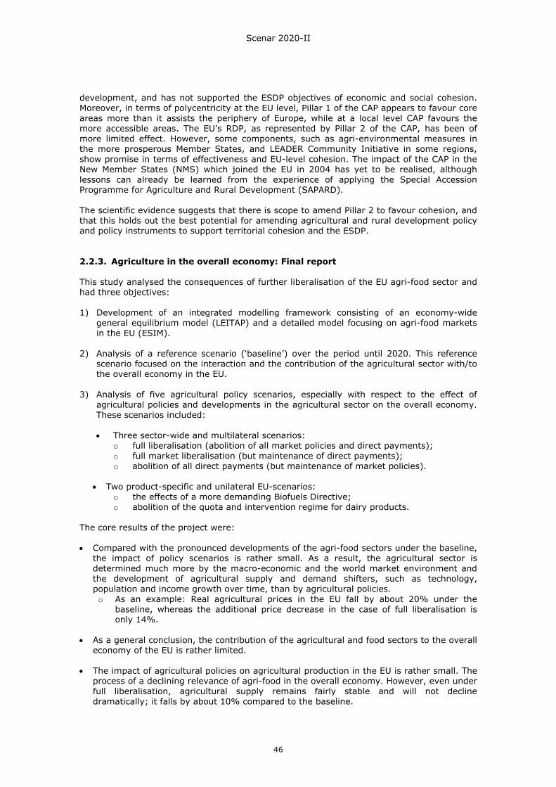
Scenar 2020-II

46

development, and has not supported the ESDP objectives of economic and social cohesion. Moreover, in terms of polycentricity at the EU level, Pillar 1 of the CAP appears to favour core areas more than it assists the periphery of Europe, while at a local level CAP favours the more accessible areas. The EU’s RDP, as represented by Pillar 2 of the CAP, has been of more limited effect. However, some components, such as agri-environmental measures in the more prosperous Member States, and LEADER Community Initiative in some regions, show promise in terms of effectiveness and EU-level cohesion. The impact of the CAP in the New Member States (NMS) which joined the EU in 2004 has yet to be realised, although lessons can already be learned from the experience of applying the Special Accession Programme for Agriculture and Rural Development (SAPARD). The scientific evidence suggests that there is scope to amend Pillar 2 to favour cohesion, and that this holds out the best potential for amending agricultural and rural development policy and policy instruments to support territorial cohesion and the ESDP. 2.2.3. Agriculture in the overall economy: Final report This study analysed the consequences of further liberalisation of the EU agri-food sector and had three objectives: 1) Development of an integrated modelling framework consisting of an economy-wide

general equilibrium model (LEITAP) and a detailed model focusing on agri-food markets in the EU (ESIM).

2) Analysis of a reference scenario (‘baseline’) over the period until 2020. This reference

scenario focused on the interaction and the contribution of the agricultural sector with/to the overall economy in the EU.

3) Analysis of five agricultural policy scenarios, especially with respect to the effect of

agricultural policies and developments in the agricultural sector on the overall economy. These scenarios included:

• Three sector-wide and multilateral scenarios:

o full liberalisation (abolition of all market policies and direct payments); o full market liberalisation (but maintenance of direct payments); o abolition of all direct payments (but maintenance of market policies).

• Two product-specific and unilateral EU-scenarios:

o the effects of a more demanding Biofuels Directive; o abolition of the quota and intervention regime for dairy products.

The core results of the project were: • Compared with the pronounced developments of the agri-food sectors under the baseline,

the impact of policy scenarios is rather small. As a result, the agricultural sector is determined much more by the macro-economic and the world market environment and the development of agricultural supply and demand shifters, such as technology, population and income growth over time, than by agricultural policies. o As an example: Real agricultural prices in the EU fall by about 20% under the

baseline, whereas the additional price decrease in the case of full liberalisation is only 14%.

• As a general conclusion, the contribution of the agricultural and food sectors to the overall

economy of the EU is rather limited. • The impact of agricultural policies on agricultural production in the EU is rather small. The

process of a declining relevance of agri-food in the overall economy. However, even under full liberalisation, agricultural supply remains fairly stable and will not decline dramatically; it falls by about 10% compared to the baseline.

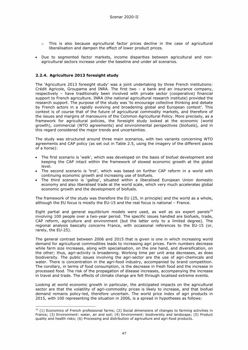
Scenar 2020-II

47

o This is also because agricultural factor prices decline in the case of agricultural liberalisation and dampen the effect of lower product prices.

• Due to segmented factor markets, income disparities between agricultural and non-

agricultural sectors increase under the baseline and under all scenarios. 2.2.4. Agriculture 2013 foresight study The ‘Agriculture 2013 foresight study’ was a joint undertaking by three French institutions: Crédit Agricole, Groupama and INRA. The first two – a bank and an insurance company, respectively – have traditionally been involved with private sector (cooperative) financial support to French agriculture. INRA (the national agricultural research institute) provided the research support. The purpose of the study was ‘to encourage collective thinking and debate by French actors in a rapidly evolving and broadening global and European context’. This context is of course that of the future of agricultural commodity markets, and therefore of the issues and margins of manoeuvre of the Common Agricultural Policy. More precisely, as a framework for agricultural policies, the foresight study looked at the economic (world growth), commercial (WTO agreements) and environmental perspectives (biofuels), and in this regard considered the major trends and uncertainties. The study was structured around three main scenarios, with two variants concerning WTO agreements and CAP policy (as set out in Table 2.5, using the imagery of the different paces of a horse): • The first scenario is ‘walk’, which was developed on the basis of biofuel development and

keeping the CAP intact within the framework of slowed economic growth at the global level.

• The second scenario is ‘trot’, which was based on further CAP reform in a world with continuing economic growth and increasing use of biofuels.

• The third scenario is ‘gallop’, situated within a liberalised European Union domestic economy and also liberalised trade at the world scale, which very much accelerates global economic growth and the development of biofuels.

The framework of the study was therefore the EU (25, in principle) and the world as a whole, although the EU focus is mostly the EU-15 and the real focus is national – France. Eight partial and general equilibrium models were used, as well as six expert panels10 involving 100 people over a two-year period. The specific issues handled are biofuels, trade, CAP reform, agriculture and environment (but the latter only to a limited degree). The regional analysis basically concerns France, with occasional references to the EU-15 (or, rarely, the EU-25). The general contrast between 2006 and 2015 that is given is one in which increasing world demand for agricultural commodities leads to increasing agri prices. Farm numbers decrease while farm size increases, along with specialisation, on the one hand, and diversification, on the other; thus, agri-activity is broadening. Working time per unit area decreases, as does biodiversity. The public issues involving the agri-sector are the use of agri-chemicals and water. There is concentration in the agri-food industry, accompanied by brand competition. The corollary, in terms of food consumption, is the decrease in fresh food and the increase in processed food. The risk of the propagation of disease increases, accompanying the increase in travel and trade. The effects of climate change are felt through localised extreme events. Looking at world economic growth in particular, the anticipated impacts on the agricultural sector are that the volatility of agri-commodity prices is likely to increase, and that biofuel demand remains policy-led, therefore uncertain. The world price index of agri products in 2015, with 100 representing the situation in 2006, is a spread in hypotheses as follows:

10 (1) Economics of French professional farms; (2) Social dimensions of changes to farming activities in France; (3) Environment: water, air and soil; (4) Environment: biodiversity and landscape; (5) Product quality and health risks; (6) Processing and distribution of agriculture and agri-food products.

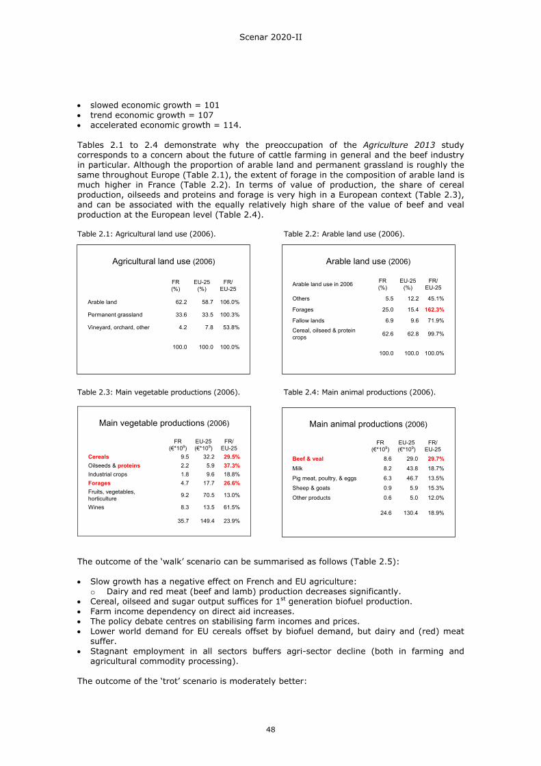
Scenar 2020-II

48

• slowed economic growth = 101 • trend economic growth = 107 • accelerated economic growth = 114. Tables 2.1 to 2.4 demonstrate why the preoccupation of the Agriculture 2013 study corresponds to a concern about the future of cattle farming in general and the beef industry in particular. Although the proportion of arable land and permanent grassland is roughly the same throughout Europe (Table 2.1), the extent of forage in the composition of arable land is much higher in France (Table 2.2). In terms of value of production, the share of cereal production, oilseeds and proteins and forage is very high in a European context (Table 2.3), and can be associated with the equally relatively high share of the value of beef and veal production at the European level (Table 2.4). Table 2.1: Agricultural land use (2006). Table 2.2: Arable land use (2006). Table 2.3: Main vegetable productions (2006). Table 2.4: Main animal productions (2006).

Main vegetable productions (2006)

23.9%149.435.7

61.5%13.58.3Wines

13.0%70.59.2Fruits, vegetables, horticulture

26.6%17.74.7Forages18.8%9.61.8Industrial crops37.3%5.92.2Oilseeds & proteins29.5%32.29.5Cereals

FR/EU-25

EU-25(€*109)

FR(€*109)

The outcome of the ‘walk’ scenario can be summarised as follows (Table 2.5): • Slow growth has a negative effect on French and EU agriculture:

o Dairy and red meat (beef and lamb) production decreases significantly. • Cereal, oilseed and sugar output suffices for 1st generation biofuel production. • Farm income dependency on direct aid increases. • The policy debate centres on stabilising farm incomes and prices. • Lower world demand for EU cereals offset by biofuel demand, but dairy and (red) meat

suffer. • Stagnant employment in all sectors buffers agri-sector decline (both in farming and

agricultural commodity processing). The outcome of the ‘trot’ scenario is moderately better:

Arable land use (2006)

100.0%100.0100.0

99.7%62.862.6Cereal, oilseed & protein crops

71.9%9.66.9Fallow lands

162.3%15.425.0Forages

45.1%12.25.5Others

FR/EU-25

EU-25(%)

FR(%)Arable land use in 2006

Agricultural land use (2006)

100.0%100.0100.0

53.8%7.84.2Vineyard, orchard, other

100.3%33.533.6Permanent grassland

106.0%58.762.2Arable land

FR/EU-25

EU-25(%)

FR(%)

Main animal productions (2006)

18.9%130.424.6

12.0%5.00.6Other products

15.3%5.90.9Sheep & goats

13.5%46.76.3Pig meat, poultry, & eggs

18.7%43.88.2Milk

29.7%29.08.6Beef & veal

FR/EU-25

EU-25(€*109)

FR(€*109)

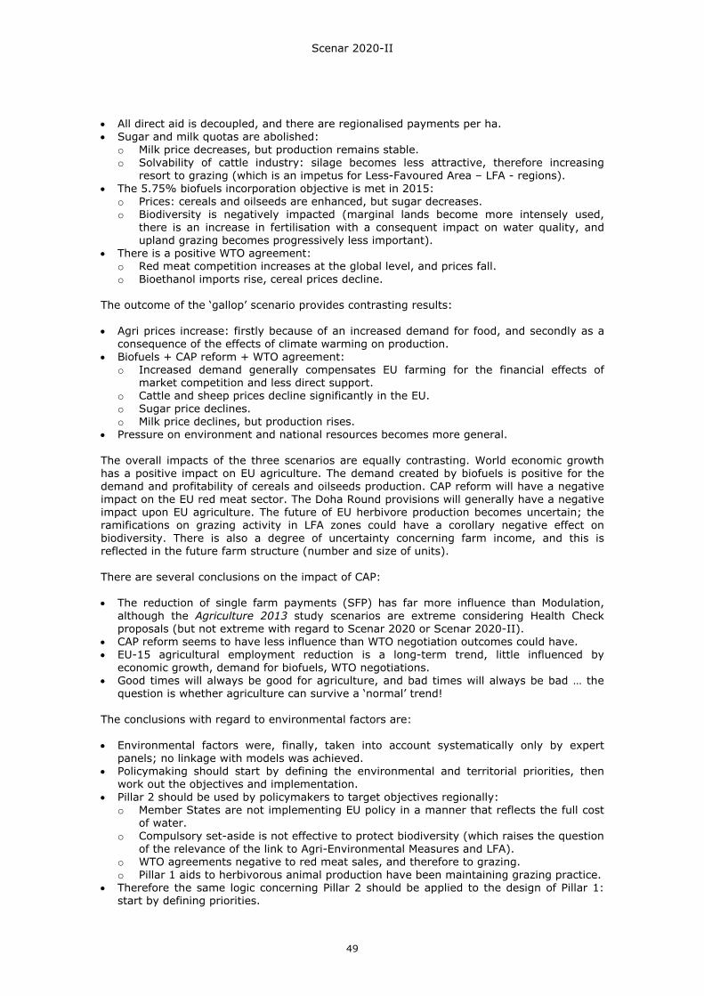
Scenar 2020-II

49

• All direct aid is decoupled, and there are regionalised payments per ha. • Sugar and milk quotas are abolished:

o Milk price decreases, but production remains stable. o Solvability of cattle industry: silage becomes less attractive, therefore increasing

resort to grazing (which is an impetus for Less-Favoured Area – LFA - regions). • The 5.75% biofuels incorporation objective is met in 2015:

o Prices: cereals and oilseeds are enhanced, but sugar decreases. o Biodiversity is negatively impacted (marginal lands become more intensely used,

there is an increase in fertilisation with a consequent impact on water quality, and upland grazing becomes progressively less important).

• There is a positive WTO agreement: o Red meat competition increases at the global level, and prices fall. o Bioethanol imports rise, cereal prices decline.

The outcome of the ‘gallop’ scenario provides contrasting results: • Agri prices increase: firstly because of an increased demand for food, and secondly as a

consequence of the effects of climate warming on production. • Biofuels + CAP reform + WTO agreement:

o Increased demand generally compensates EU farming for the financial effects of market competition and less direct support.

o Cattle and sheep prices decline significantly in the EU. o Sugar price declines. o Milk price declines, but production rises.

• Pressure on environment and national resources becomes more general. The overall impacts of the three scenarios are equally contrasting. World economic growth has a positive impact on EU agriculture. The demand created by biofuels is positive for the demand and profitability of cereals and oilseeds production. CAP reform will have a negative impact on the EU red meat sector. The Doha Round provisions will generally have a negative impact upon EU agriculture. The future of EU herbivore production becomes uncertain; the ramifications on grazing activity in LFA zones could have a corollary negative effect on biodiversity. There is also a degree of uncertainty concerning farm income, and this is reflected in the future farm structure (number and size of units). There are several conclusions on the impact of CAP: • The reduction of single farm payments (SFP) has far more influence than Modulation,

although the Agriculture 2013 study scenarios are extreme considering Health Check proposals (but not extreme with regard to Scenar 2020 or Scenar 2020-II).

• CAP reform seems to have less influence than WTO negotiation outcomes could have. • EU-15 agricultural employment reduction is a long-term trend, little influenced by

economic growth, demand for biofuels, WTO negotiations. • Good times will always be good for agriculture, and bad times will always be bad … the

question is whether agriculture can survive a ‘normal’ trend! The conclusions with regard to environmental factors are: • Environmental factors were, finally, taken into account systematically only by expert

panels; no linkage with models was achieved. • Policymaking should start by defining the environmental and territorial priorities, then

work out the objectives and implementation. • Pillar 2 should be used by policymakers to target objectives regionally:

o Member States are not implementing EU policy in a manner that reflects the full cost of water.

o Compulsory set-aside is not effective to protect biodiversity (which raises the question of the relevance of the link to Agri-Environmental Measures and LFA).

o WTO agreements negative to red meat sales, and therefore to grazing. o Pillar 1 aids to herbivorous animal production have been maintaining grazing practice.

• Therefore the same logic concerning Pillar 2 should be applied to the design of Pillar 1: start by defining priorities.

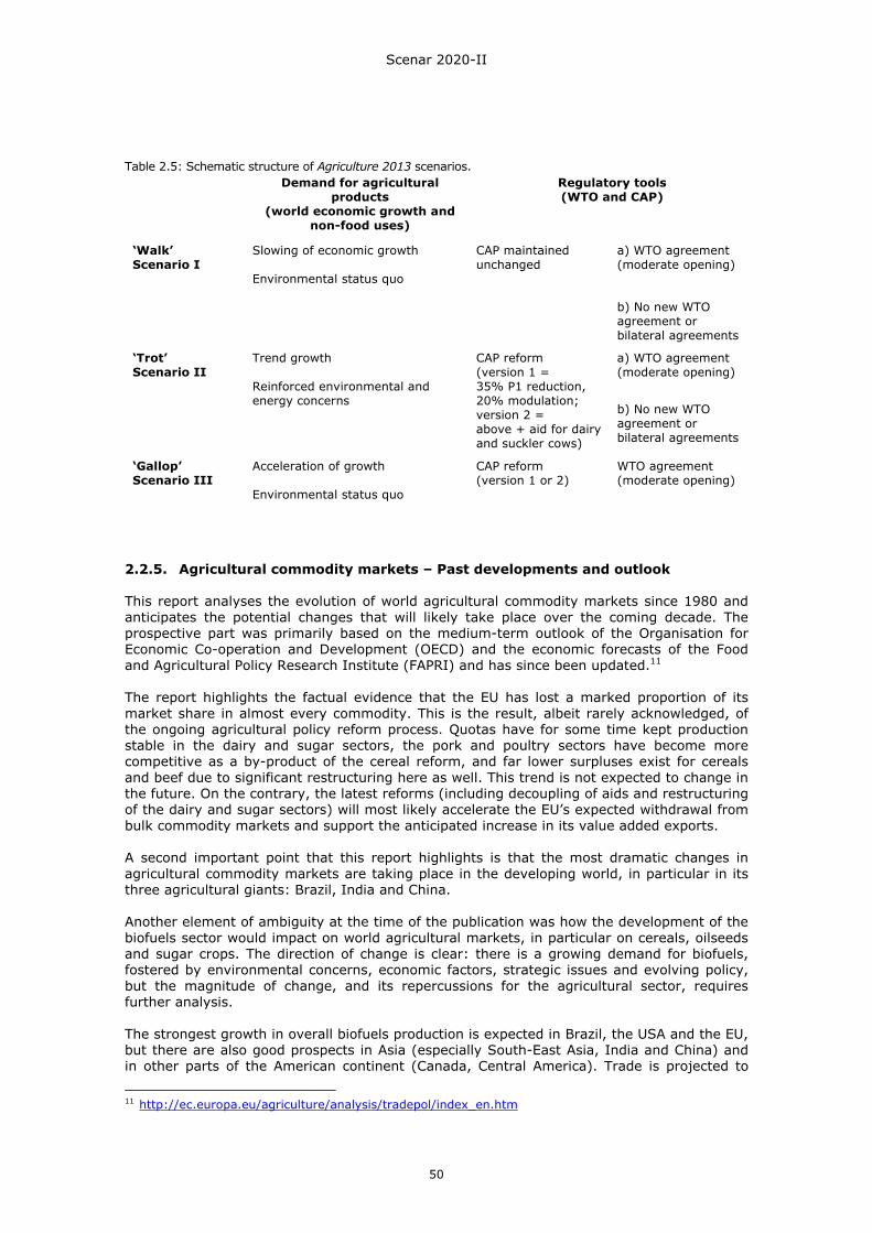
Scenar 2020-II

50

Table 2.5: Schematic structure of Agriculture 2013 scenarios. Demand for agricultural

products (world economic growth and

non-food uses)

Regulatory tools (WTO and CAP)

a) WTO agreement (moderate opening)

‘Walk’ Scenario I

Slowing of economic growth Environmental status quo

CAP maintained unchanged

b) No new WTO agreement or bilateral agreements

a) WTO agreement (moderate opening)

‘Trot’ Scenario II

Trend growth Reinforced environmental and energy concerns

CAP reform (version 1 = 35% P1 reduction, 20% modulation; version 2 = above + aid for dairy and suckler cows)

b) No new WTO agreement or bilateral agreements

‘Gallop’ Scenario III

Acceleration of growth Environmental status quo

CAP reform (version 1 or 2)

WTO agreement (moderate opening)

2.2.5. Agricultural commodity markets – Past developments and outlook This report analyses the evolution of world agricultural commodity markets since 1980 and anticipates the potential changes that will likely take place over the coming decade. The prospective part was primarily based on the medium-term outlook of the Organisation for Economic Co-operation and Development (OECD) and the economic forecasts of the Food and Agricultural Policy Research Institute (FAPRI) and has since been updated.11 The report highlights the factual evidence that the EU has lost a marked proportion of its market share in almost every commodity. This is the result, albeit rarely acknowledged, of the ongoing agricultural policy reform process. Quotas have for some time kept production stable in the dairy and sugar sectors, the pork and poultry sectors have become more competitive as a by-product of the cereal reform, and far lower surpluses exist for cereals and beef due to significant restructuring here as well. This trend is not expected to change in the future. On the contrary, the latest reforms (including decoupling of aids and restructuring of the dairy and sugar sectors) will most likely accelerate the EU’s expected withdrawal from bulk commodity markets and support the anticipated increase in its value added exports. A second important point that this report highlights is that the most dramatic changes in agricultural commodity markets are taking place in the developing world, in particular in its three agricultural giants: Brazil, India and China. Another element of ambiguity at the time of the publication was how the development of the biofuels sector would impact on world agricultural markets, in particular on cereals, oilseeds and sugar crops. The direction of change is clear: there is a growing demand for biofuels, fostered by environmental concerns, economic factors, strategic issues and evolving policy, but the magnitude of change, and its repercussions for the agricultural sector, requires further analysis. The strongest growth in overall biofuels production is expected in Brazil, the USA and the EU, but there are also good prospects in Asia (especially South-East Asia, India and China) and in other parts of the American continent (Canada, Central America). Trade is projected to

11 http://ec.europa.eu/agriculture/analysis/tradepol/index_en.htm

Scenar 2020-II

51

develop from South to North America. EU imports are set to increase following the implementation of the biofuels legislation. Asian needs are likely to be covered by regional exporters (including Australia) but also by Latin America. Palm oil exports from Malaysia and Indonesia will continue to soar and fuel uses of other oil crops are expected to develop in Asia. Some countries in Southern Africa could also export ethanol to both the Far East and the EU. The growth in biofuel uses will also contribute to enhanced demand for maize and oilseeds. These commodities already benefit from sustained demand for feed and/or food uses and this is expected to continue under the outlook projections. In the case of oilseeds, the competition between food and fuel uses will become more marked for oil, oilmeals being a co-product in both cases. In the case of maize, it is more a trade-off between feed and other non-food uses which means a link has to be made to the outlook for the livestock sector as well. This link is also relevant to trade analysis because a decline in the export of grains or meals can in turn translate into higher exports of meat. One final point concerning the meat sector is the fact that the outlook – as established in 2005 – was rather optimistic. Although the beef sector is expected to grow faster than it has in past decades, the growth rate in the pig meat and poultry sectors is expected to slow down and recent history shows unexpected animal health epidemics can have serious, unpredictable and lasting repercussions on agricultural markets, particularly the sector they directly affect. In particular, the spread of avian influenza has the potential to cause the first major disruption of the world poultry sector, with significant negative knock-on effects for the feed cereals and oilseed/meals markets. 2.2.6. OECD-FAO Agricultural outlook 2008–2017 The 2008–2017 edition was the fourth time that the Agricultural Outlook report has been prepared jointly by the Organisation for Economic Co-operation and Development (OECD) and the Food and Agriculture Organization (FAO) of the United Nations. The report drew on the commodity, policy and country expertise of both organisations to provide a longer-term assessment of future prospects in the major world agricultural commodity markets. The 2008–2017 edition of the Agricultural Outlook offered an assessment of agricultural markets covering cereals, oilseeds, sugar, meats, milk and dairy products over the period 2008 to 2017. For the first time, it also included an analysis of and projections for global biofuel markets for bioethanol and biodiesel, facilitating the discussion of interactions between these markets and those for the main agricultural feedstocks used in their production. The Agricultural Outlook 2008–2017 presents a plausible scenario for the evolution of agricultural markets over the next decade and provides a benchmark for the analysis of agricultural market outcomes that would result from alternative economic or policy assumptions. The Agricultural Outlook 2008–2017 was set against a backdrop of exceptional increases in prices for many agricultural commodities, which posed a considerable challenge in preparing the projections and assessing the ‘durability’ of the various influences shaping these prices. The report provides the following outlook: • World reference prices in nominal terms for almost all agricultural commodities covered in

this report are at or above previous record levels. There is strong reason to believe that there are now also permanent factors underpinning prices that will work to keep them both at higher average levels than in the past and reduce the long-term decline in real terms.

• The dramatic increase in prices since 2005/06 is partly the result of adverse weather

conditions in major grain-producing regions in the world, with spill-over effects on crops and livestock that compete for the same land. In a context of low global stocks, these developments alone would have triggered strong price reactions. These conditions are not new; they have happened in the past and prices came down once more normal conditions

Scenar 2020-II

52

prevailed and supply responded over time. The Agricultural Outlook 2008–2017 saw no reason to believe that this will not recur over the next few years.

• The underlying forces that drive agricultural product supply (by and large productivity

gains) will eventually outweigh the forces that determine stronger demand, both for food and feed as well as for industrial demand, most notably for biofuel production. As a result of these dynamics in supply and demand, the Agricultural Outlook 2008–2017 suggested that commodity prices – in nominal terms – over the medium term will average substantially above the levels that prevailed in the previous 10 years. When the average for 2008–2017 is compared with that over 1998–2007, beef and pork prices may be some 20% higher; raw and white sugar around 30%; wheat, maize and skim-milk powder 40 to 60%; butter and oilseeds more than 60% and vegetable oils over 80%. Over the Agricultural Outlook 2008–2017 period, prices will resume their decline in real terms, albeit at a slower rate. However, the impact of various supply and demand factors on prices will differ across commodities.

• On the supply side, the Agricultural Outlook 2008–2017 expected continued yield growth

for crops to be more important than new areas brought into cultivation in determining crop supply. Slowly increasing dairy and livestock yields also support the increase in milk and meat production. A key assumption in the Agricultural Outlook 2008–2017 is some strengthening of the US dollar against most currencies. In the countries affected by this change, this will reinforce domestic price incentives to increase production. These factors combine to sustain the growth of global agricultural production, although some of that impetus is abated by the supply-reducing effect of high oil prices that raise production costs.

• On the demand side, changing diets, urbanisation, economic growth and expanding

populations are driving food and feed demand in developing countries. Globally, and in absolute terms, food and feed remain the largest sources of demand growth in agriculture. But stacked on top of this is now the fast-growing demand for feedstock to fuel a growing bioenergy sector. While smaller than the increase in food and feed use, biofuel demand is the largest source of new demand in decades and a strong factor underpinning the upward shift in agricultural commodity prices.

• As a result of these dynamics in supply and demand, the Agricultural Outlook 2008–2017

suggested that commodity prices – in nominal terms – over the medium term will average substantially above the levels that prevailed in the previous 10 years. When the average for 2008 to 2017 is compared with that over 1998 to 2007, beef and pork prices may be some 20% higher; raw and white sugar around 30%; wheat, maize and skim-milk powder 40 to 60%; butter and oilseeds more than 60% and vegetable oils over 80%. Over the Agricultural Outlook 2008–2017 period, prices will resume their decline in real terms, albeit at a slower rate. However, the impact of various supply and demand factors on prices will differ across commodities.

• In addition, prices may also be more volatile than in the past: stock levels are not

expected to be replenished substantially over the period covered by the Agricultural Outlook 2008–2017; demand is becoming less sensitive to price changes at the farm level as the commodity share in the final food bill falls and as industrial demand grows; weather conditions and agricultural product supply may become more variable with climate change; and speculative non-commercial investment funds enter or leave agricultural futures markets as profit opportunities dictate.

• Within this overall context, the epicentre of global agriculture will further shift from the

OECD towards developing countries. Both consumption and production are growing faster in developing countries for all products except wheat. By 2017, these countries are expected to dominate production and consumption of most commodities, with the exception of coarse grains, cheese and skim-milk powder.

• Corresponding shifts are also occurring in global trade patterns. Imports are growing

most in developing countries, and an increasing share of this growth is captured by larger exports from other emerging and developing countries. Export growth in developing

Scenar 2020-II

53

countries is greater, and sometimes very much so for almost all products. However, while the share of OECD countries in world exports falls, these countries continue to dominate export trade for wheat, coarse grains, pork and all dairy products.

• High prices are good for some and bad for others. They are beneficial for many

commercial producers in both developed and developing countries. However, many farmers in developing countries are not linked to markets and will draw little or no benefit from currently higher prices. But the poor, and in particular the urban poor in net food importing developing countries, will suffer more. In many low-income countries, food expenditures average over 50% of income and the higher prices contained in the Agricultural Outlook 2008–2017 will push more people into undernourishment.

• For the Least Developed Countries, especially the food-deficit group, the projections thus

show greatly increased vulnerability and uncertain food supplies during an era of high commodity prices and high price volatility. This underscores the importance of developing their domestic supply capacity by improving the overall environment in which agriculture operates through enhancing governance and administrative systems and investing in education, training and extension services, research and development (R&D) and physical infrastructure. While these are longer-term remedies, it is important in the short term that commodity trade functions efficiently to facilitate the allocation of available commodity supplies.

• The Agricultural Outlook 2008–2017 assumed unchanged agricultural and trade policies.

The actual evolution of agricultural commodity and food prices, however, hinges importantly on future policy developments. In this context, increased humanitarian aid is needed to reduce the negative impact of high prices on the very poor, and this could be done without any major impact on markets.

• Such effects would result, however, from trade-restricting policies such as export taxes

and embargoes. These may in the short term provide some relief to domestic consumers but in fact impose a burden on domestic producers and limit their supply response, as well as contribute to global commodity market uncertainty. Similarly, measures to protect domestic producers of agricultural commodities through border measures impose a burden on domestic consumers; it would also restrict growth opportunities for producers abroad.

• Policy support, as well as oil-price developments, will strongly influence the evolution of

future demand from biofuels for agricultural commodity feedstocks. In this context, neither the US Energy Independence and Security Act (EISA) nor proposals for a new EU Bioenergy Directive are taken into account. Changes in either, or new technological developments would also have a strong impact on projected world prices for agricultural commodities and for the availability for food and feed use. In the Agricultural Outlook 2008–2017, 2nd generation biofuels are not expected to be produced on a commercial basis over the Outlook period.

• Finally, over the longer term, agricultural supply is facing increased uncertainties and

limitations to the amount of new land that can be taken into cultivation. Public and private investments in innovation and increasing agricultural productivity, particularly in developing countries, would greatly improve supply prospects by helping to broaden the production base and lessen the chance of recurring commodity price spikes.

• The Agricultural Outlook 2008–2017 was prepared in an environment characterised by

increased instability in financial markets, higher food price inflation, signs of weakening global economic growth and food-security concerns. Although projections for agricultural commodity markets have always been subject to a number of uncertainties, these took on more importance in this edition of the Agricultural Outlook.

Scenar 2020-II

54

2.2.7. Regions 2020: An assessment of future challenges for EU regions The aim of this document was to examine the extent to which Community policies are adapted to challenges that European regions will face in the coming years and what the role of Community policies should be in responding to these challenges. The following four challenges may be of particular relevance for European regions: • Globalisation is driving scientific and technological progress, making the European

dimension ever more important in boosting knowledge, mobility, competitiveness and innovation. The opening up of huge new markets creates vast new opportunities for Europeans, but it will at the same time test Europe's capacity to further adjust to structural change and manage the social consequences of that change. The transformation to a knowledge and service economy is as profound as the earlier change-over from agriculture to industry.

• Demographic change will transform the age and employment structure of our societies,

raising important issues of both economic efficiency and intergenerational equity. Migratory pressure will have a particularly strong effect on Europe, due to its proximity to some of the world's poorest regions and those likely to be worst affected by climate change and natural resource constraints.

• The impact of climate change on Europe's environment and its society has become central

to the European agenda, challenging policymakers to reflect on how best to respond with the policy instruments at the EU's disposal. This applies both to efforts to mitigate climate change by tackling the growth in greenhouse gas emissions and to the need for measures to adapt to the consequences of climate change.

• Secure, sustainable and competitive energy represents one of society's main challenges.

Limited supply, increased global demand and the imperative to cut emissions have led to a new realisation of the need to move towards a low-carbon economy in Europe.

Together these challenges will impact on the development of Europe's economies and societies over the coming years. The Regions 2020 study sought to explore the regional effects of these challenges in the medium-term perspective of 2020. It sought to illustrate which regions are most vulnerable to these challenges, as a step towards a better understanding of the potential pattern of regional disparities that these challenges will generate. Europe will face a number of key challenges in the years to come, including: adapting to globalisation, demographic change, climate change and the energy challenge. All European regions will be affected. However, each of the challenges exhibits a distinct pattern. With the exception of energy, all challenges display strong subnational variations: • For globalisation, southern and south-eastern regions appear to be highly vulnerable, but

considerable variations can be observed in both Germany and the new Member States. • For demographic change, there is significant variation across European regions, once

again with slightly greater vulnerability in southern and south-eastern regions. However, it should be stressed that there is a lag in the demographic transition of the new Member States and that the effects will be very similar in the next generation to those already seen in the old Member States.

Examining the combination of these challenges provides interesting results: • As regards socio-economic challenges, some regions appear to be favourably placed to

benefit from globalisation, but face the risk of demographic decline. These regions are located in Central France, Eastern Germany, parts of Sweden and Finland, as well as in some new Member States. A number of regions – mainly located in Southern Europe – appear to be vulnerable to both challenges. At subnational level, metropolitan areas seem to be better equipped than remote rural areas to face both types of challenge. It is thus

Scenar 2020-II

55

difficult to predict how these challenges will interact and what conclusions can be drawn in terms of future developments.

• Climate change and the energy challenge will affect all regions. Regions in the

Mediterranean part of Europe seem to be more exposed to these challenges, whereas northern and western European regions appear to be less at risk. However, the impact depends on climate change scenarios which may vary considerably over time. Energy dependence clearly follows national patterns, without showing a clear East–West or North–South divide. Developments will depend on the European Union's capacity to develop a common policy on energy ensuring the functioning of the internal market and security of energy supply.

A synthetic index was developed to further illustrate the geography of these multiple challenges. The index classifies in very broad terms how many challenges will affect each European region. It provides an overview of the top 50% of regions most affected by each individual challenge, indicating risk intensity. Most regions expected to be intensively affected by three or more challenges at the same time are located in Southern Europe and on the coasts of Western and Central Europe. Regions with fewer simultaneous challenges are relatively close to the geographical core of the EU, but are also located in Southern Spain, the UK, Ireland, Denmark, Sweden, Finland and Lithuania. Most of the impacts of the four challenges will be expressed in different ways according to the particular region and are likely to create regional disparities. Some of the challenges tend to be more closely interlinked than others. Globalisation, demographic change and aspects of energy and climate change have distinct impacts on the economy and regional growth potential, as well as on social polarisation. For example, overly volatile energy prices could adversely affect the competitiveness and regional growth potential of regions with inefficient energy use and high reliance on transport. As a consequence, households might be adversely affected by higher unemployment as well as by temporarily higher spending on energy. Growing social polarisation could be the result. Certain challenges, therefore, might reinforce each other. Other combinations of challenges might have a lower impact. Demographic change and globalisation may have a more limited impact on environmental sustainability than energy and climate change. The interaction of various challenges is, thus, extremely complex. Moreover, as noted above, the projections made in the report did not take into account a number of factors which may be decisive, such as the capacity of the regions, the Member States, and the European Union to respond, notably on the basis of further technological development. Through their cohesion programmes in 2007–2013, for example, some Member States and regions, in partnership with the Commission, are endeavouring to contribute towards tackling these challenges. The question how EU policies, including cohesion policy, can best contribute to addressing those challenges in the next decade and beyond, whilst fully taking solidarity and sustainability aspects into account, will be a key issue of the ongoing review of the EU budget. 2.2.8. Alternative futures of rural areas in the EU The aim of this study was to explore alternative futures of rural areas in the EU. For this purpose, a comparative analysis of seven scenario studies of rural areas in the EU was conducted: ESPON, Eururalis, Scenar 2020, SEAMLESS, SENSOR, PRELUDE and Agriculture in the overall economy. This analysis was used to identify a set of alternative futures of rural areas in the EU that are often used in the scenario studies and cover a wide range of different possible futures. The time horizon in this study was not fixed, but depended on the time horizon used in the studies under review. Often, the reviewed scenario studies constructed a baseline scenario – derived from an extrapolation of past trends and policies – and a number of alternative scenarios with different degrees of policy intervention. Usually, these alternatives refer to a liberalisation

Scenar 2020-II

56

scenario with a low degree of policy regulation and a cohesion scenario with a high degree of policy regulation. The construction of scenarios in PRELUDE and Eururalis, however, deviates from the other scenario studies. PRELUDE does not use a baseline scenario and alternative policy scenarios, but assumes a number of disruptive events in the near future. These events provoke a series of ‘new’ population and policy responses, resulting in images of the rural future in Europe that strongly deviate from the present situation in rural Europe. Eururalis also does not use a baseline scenario, but employs a set of four contrasting futures, derived from opposite dimensions of policy intervention and global market integration. The precise meaning of ‘rural areas’ differs among the scenario studies, varying from a wide territorial approach to a more narrow sectoral approach. Often, the time horizon in these studies refers to 2020 or 2030. Depending on the assumptions made in the scenarios, smaller or larger changes in rural areas in the EU are anticipated in comparison with the current situation. On the whole, by focusing on population, globalisation, climate change, policies, agriculture, agricultural land use, landscape, nature and biodiversity and territorial disparities in rural Europe, six distinct alternative images of rural areas in Europe were derived from the scenario studies. These could successively be labelled as: 1) Rural future in the EU: baseline. 2) Rural future in the EU: liberalisation. 3) Rural future in the EU: cohesion. 4) Rural future in the EU: clustered networks. 5) Rural future in the EU: lettuce surprise u. 6) Rural future in the EU: big crisis. The images of a liberalised (competitive) and cohesion rural future reflect a dichotomy in regional development policies of efficiency versus equity. However, rural images like clustered networks, lettuce surprise u and big crisis reveal that the main challenges for Europe’s rural future are not contained within this dichotomy of competitiveness versus cohesion. On the contrary, these challenges require new policy approaches, that might depart in many respects from the policies applied up to now. Moreover, the role of public policies in shaping the rural future should not be exaggerated. Rural Europe rather emerges from the interplay of global market forces and local responses by entrepreneurs, consumers and policymakers. 2.2.9. Impact of EU biofuel policies on world agricultural and food markets This paper assesses the global and sectoral implications of the EU Biofuels Directive in a multi-region computable general equilibrium framework. Until now biofuels have been produced by processing agricultural crops using available technologies. These so-called 1st generation biofuels can be used in low percentage blends with conventional fuels in most vehicles and can be distributed through existing infrastructure. Advanced conversion technologies are needed for a second generation of biofuels. The second generation will use a wider range of biomass resources – agriculture, forestry and waste materials – and promises to achieve higher reductions in greenhouse gas emissions and the costs of fuel production. Given the current policy developments and the availability of just 1st generation biofuels, an increased biofuel production due to either ‘pure’ market forces and/or ‘policy’ might have significant impacts on agricultural markets, including world prices, production, trade flow, and land use. Linkages between food and energy production include the competition for land, but also for other production inputs. The effect of an increasing supply of by-products of biofuel production, such as oil cake and gluten feed, also affects animal production, for example. Furthermore, the biofuel boom has raised concerns such as whether biofuels will hurt the poor by increasing food prices or whether it will lead to biodiversity loss due to increased land use. All these implications are not well understood and this study tries to address these issues.

Scenar 2020-II

57

More specifically, the purpose of this paper was to assess the global and sectoral implications of the EU Biofuels Directive (European Commission, 2003), in a multi-region computable general equilibrium framework. This Directive states that the EU Member States should ensure that biofuels and other renewable fuels attain a minimum share of their total consumption of transport fuel, which is responsible for almost 25% of all greenhouse gas emissions in the EU. This share should lie, measured in terms of energy content, at 5.75% by the end of 2010. These goals are not yet mandatory, but this could change and a discussion about higher shares in the future is ongoing. With this focus on the impact of the EU Biofuels Directive on production, land use and trade this paper contributes to the current discussion on the growing competition between agricultural products used for food, feed and fuel purposes. This study shows that enhanced demand for biofuel crops under the EU Biofuels Directive has a strong impact on agriculture at global and European levels. The long-term trend of declining real world prices of agricultural products slows down or might even be reversed for the feedstocks used for biofuels. The incentive to increase production in the EU will tend to increase land prices and farm income in the EU and other regions. The EU will not be able to produce domestically the feedstocks needed to produce the biofuels according to the Biofuels Directive and will run into a higher agricultural trade deficit. Biofuel crop production is expanding in other highly industrialised countries and especially in South and Central America (Brazil). The results depend heavily on the development of the price of crude oil. The higher the crude oil price, the more competitive biofuel crops become in petroleum production. Without mandatory blending or subsidies to stimulate the use of biofuel crops in the petroleum sector, the targets of the EU Biofuels Directive will not be reached in 2010. A mandatory blending leads to higher petrol prices as feedstocks are not profitable to use in fuel production given the current technologies. The increased demand for feedstocks raises their price relative to the oil price and therefore adds to the challenge of making biofuels competitive. Therefore, if biofuels have to be competitive in the long run, investments in R&D are needed to obtain higher yields or better conversion technologies. However, in this paper the analysis focuses only on 1st generation biofuels as the focus is on the period until 2010. Decisions on R&D investments should take the 2nd generation biofuels into account, as they promise to be more cost effective and more effective in reducing greenhouse gas emissions. 2.2.10. Final report on the project ‘Sustainable Agriculture and Soil Conservation

(SoCo)’ Agriculture occupies a substantial proportion of the European land area, and consequently plays an important role in maintaining natural resources and cultural landscapes, a precondition for other human activities in rural areas. Unsustainable farming practices and land use, including inappropriate intensification and land abandonment, have an adverse impact on natural resources. Having recognised the environmental challenges of agricultural land use, in 2007 the European Parliament requested the European Commission to carry out the pilot project ‘Sustainable agriculture and soil conservation through simplified cultivation techniques (SoCo)’. The project originated from a close cooperation between the Directorate-General for Agriculture and Rural Development (DG AGRI) and the Joint Research Centre (JRC). It was carried out by the Institute for Prospective Technological Studies (IPTS) and the Institute for Environment and Sustainability (IES). The overall objectives of the SoCo project were: (i) to improve the understanding of soil conservation practices in agriculture and their links with other environmental objectives; (ii) to analyse how farmers can be encouraged, through appropriate policy measures, to adopt soil conservation practices; and (iii) to make this information available to relevant stakeholders and policymakers in an EU-wide context. Regarding the first objective, a stock-taking was conducted throughout the EU, collecting information via a literature review, the use of parametric and empirical models, and a survey of policy measures. The second objective was mainly achieved by ten case studies across the

Scenar 2020-II

58

EU and a series of regional workshops. The third objective was met through the final report and the planned dissemination process. The final report synthesises the findings of the SoCo project and translates them into conclusions and recommendations. Nature, location and magnitude of soil degradation processes related to agriculture Soil is subject to a series of degradation processes. Six of the soil degradation processes recognised at EU level (water, wind and tillage erosion; decline of soil organic carbon; compaction; salinisation and sodification; contamination; and declining soil biodiversity) are closely linked to agriculture. Within SoCo, the magnitude of the related soil degradation risks was estimated at EU level, and areas where these risks are most likely to occur were identified. Risk was assessed through parametric and empirical models and, thus, the assessment should not be interpreted with the same accuracy as field measurements. The major drivers for water erosion are intense rainfall, topography, low soil organic matter content, percentage of vegetation cover and land marginalisation or abandonment. Several areas with a high risk of erosion (including some hotspots) are located in the Mediterranean. The highest number of erosive days on bare soil per year, posing a wind erosion risk, is found across the sand belt covering south-east England, the Netherlands, northern Germany and Poland. Apart from soil characteristics (such as soil texture), soil organic carbon decline is determined by land use, climate (mainly temperature and precipitation) and soil hydrology. The analysis shows that agricultural soils in Europe have very different actual soil organic carbon levels and are subject to different risk levels of soil organic carbon decline. There are more than 70 billion tonnes of organic carbon in EU soils, as compared to about 2 billion tonnes of carbon altogether emitted by the Member States annually. Releasing just a small fraction of the carbon currently stocked in European soils to the atmosphere could wipe out emission savings in other sectors of the economy. Therefore, maintaining and optimising organic carbon levels through proper land management can make an important contribution to climate change mitigation. European agricultural soils have a predominantly low or medium natural susceptibility to compaction. The natural susceptibility of soils to compaction mainly depends on soil texture, with sandy soils being least susceptible and clay soils being the most. The main natural factors influencing soil salinisation and sodification are climate, the salt content of soil parent material and groundwater, land cover and topography. The countries most affected by salinity or sodicity are Spain, Hungary and Romania. SoCo was not able to produce comprehensive risk assessments of the degree of soil contamination (by heavy metals and pesticides; excess of nitrates and phosphates) or declining soil biodiversity due to a lack of data. Relevant farming practices for soil protection, conservation and improvement; their uptake and related environmental objectives The SoCo final report focused its review on two specific farming systems, namely conservation agriculture and organic farming, along with a range of farming practices. The review considered their impact on soil quality and assessed, as far as possible, the uptake and benefit-cost effects in a broader sense. No-tillage and reduced tillage, in combination with cover crops and crop rotation, are essential practices in conservation agriculture. Within the EU-27, Finland and Greece show the highest uptake of no-tillage (more than 4.5% of total arable land), while reduced tillage is practised on 40 to 55% of the arable land in both Finland and the UK. Organic farming, although different from conservation agriculture, has similar positive effects on soil organic carbon content and soil biodiversity. Over the period 1998–2005, the area under organic farming (including conversion areas) certified under Council Regulation 2092/91/EEC increased by 130% in the EU-15, and by 2005 it amounted to 4% of the total Utilised Agricultural Area in the EU-25. The SoCo final report further reviewed the following specific farming practices: ridge tillage, buffer strips, contour farming, intercropping, subsoiling, terracing, and grassland establishment and maintenance. Review of the regulatory environment and policy instruments that address soil degradation To date, soil protection is not a specific objective of any EU legislation but it features in some legislation as a secondary objective. Currently, the most important EU environmental directives with respect to soil quality are the Nitrates Directive and the Water Framework

Scenar 2020-II

59

Directive. Others, such as the Birds and Habitats Directives, the Sewage Sludge Directive and the Plant Protection Products Directive, are expected to have beneficial effects on soil quality, but to a lesser extent owing to a more focused set of objectives. In the framework of the Cardiff Process, environmental objectives are to be integrated into EU sectoral policies, including the Common Agricultural Policy (CAP). The CAP comprises two principal policy directions: market price support and direct income payments (Pillar 1), and a range of selective payments for rural development measures (Pillar 2). Cross compliance, a horizontal tool for both Pillars and compulsory since 2005, plays an important role in soil protection and conservation. The Statutory Management Requirements (SMRs) create synergies between the direct payment scheme and the need to ensure compliance with a number of relevant EU environmental directives, including the Nitrates Directive. The requirement to keep agricultural land (whether in productive use or not) in good agricultural and environmental condition (GAEC) aims at preventing land abandonment and at ensuring a minimum maintenance of agricultural land. The elements of GAEC specifically target protection against soil erosion, maintenance or improvement of soil organic matter, and maintenance of a good soil structure. SoCo conducted a survey of policy implementation at Member State and regional levels across the EU-27, which was extensive but not fully comprehensive. The results indicated that the existing policy measures have the potential to address all recognised soil degradation processes across the EU, although not all policy measures are implemented in all Member States or regions, nor are they implemented in the same way. Typically, policy intervention in soil conservation is either through support for beneficial farming practices, or through the prevention or prohibition of damaging practices. A range of factors appear to influence the impact of different policy instruments. Compliance with mandatory measures and the uptake of voluntary incentive-based measures, in particular, are both strengthened through increasing awareness and advice. However, a lack of monitoring and of a (quantitative) database prevented the comprehensive evaluation of the impact, effectiveness and efficiency of the different policy measures at the time of the project. Establishment of a classification of the conservation practices and policy measures SoCo established a classification of soil conservation practices and related policy measures. It provided a schematic representation of the (likely) effects of farming systems (organic and conservation agriculture) and farming practices on soil degradation processes and related environmental issues, as well as indicating which policy measures encourage the adoption of such practices. The survey on the implementation of EU policies at Member State or regional level did not illuminate the extent to which the links between farm technical requirements and soil degradation processes are based on actual measurements. Given differences in the use and implementation of policy measures, these hypothesised cause-and-effect models may not reflect what happens on the ground in the diverse and more complex agri-environment reality. Synthesis of land management practices and policy measures at the regional level: case studies In order to reach a sufficiently detailed level of analysis and to respond to the diversity of European regions, a case study approach was applied. Ten case studies were carried out in Belgium, Bulgaria, the Czech Republic, Denmark, France, Germany, Greece, Italy, Spain and the United Kingdom between spring and summer 2008. The selection of case study areas was designed to capture differences in soil degradation processes, soil types, climatic conditions, farm structures and farming practices, institutional settings and policy priorities. There is considerable physical and spatial variability in the soil degradation processes analysed, which are not uniform even within relatively small areas. This is because the nature and extent of a degradation process is typically influenced by two interacting elements, namely the physical, environmental conditions in a given locality and the farming practices adopted. The case studies further identified some of the complex causal chains between factors that shape the adoption of different farming systems and practices, and the ultimate impacts on agricultural soils. Some drivers are economic, such as agricultural commodity prices and energy prices; others are socio-cultural and technological, such as the

Scenar 2020-II

60

trend towards use of larger and heavier machinery to increase the efficiency of field operations. Modelling environmental benefits of adopting soil conservation practices In order to assess the potential environmental benefits of adopting agricultural soil conservation practices on an EU-wide scale, the Erosion-Productivity Impact Calculator (EPIC) was used to simulate two scenarios over the period 1990–2004. The first scenario assumed adoption of no-tillage practices for producing barley and the second, the introduction of a cover crop before maize is sown. The results of the scenarios were compared to those under conventional agricultural practices (ploughing and no cover crop). The modelling supported the general conclusion that long-term policies aiming at a widespread adoption of conservation agriculture practices (no-tillage and cover crop) will reduce soil erosion effectively in most regions of the EU. The effectiveness of the policy framework for soil conservation The SoCo study showed that the existing suite of policy measures, including mechanisms for advice and support, is in general adequate for addressing soil degradation processes in the EU. The effectiveness of the policy measures could be significantly increased if the reference level were clearly defined, if incentive payments were better targeted and monitored, if greater levels of advice and support were provided, and if all relevant policy measures were coordinated and specifically targeted to soil protection. Effectiveness and efficiency A wide range of farming practices are available to farmers throughout the EU for mitigating or even reversing soil degradation processes. The case studies and the EU-wide stock-taking exercise resulted in a detailed synthesis establishing and analysing the interrelation of farming practices and soil quality in the context of the current policy setting. However, the issue of which farming practices are preferable or should be further promoted to avoid or mitigate soil degradation processes needs further investigation. Generally, controlling the soil degradation process itself, rather than mitigating its off-site effect, is regarded as more effective, even though the result might not be immediate. Information and advice are essential to support any changes in farming practices. Farm advisory services should support the implementation of farming practices aimed at sustainable soil use. However, stakeholders in nearly all case study regions mentioned the lack of routine advice and encouragement for farmers to practise soil conservation. Recommendations The EU-wide stock-taking exercise and the case study analysis showed that there is a range of measures within the current European Agricultural Fund for Rural Development (EAFRD) that are appropriate for supporting sustainable soil management, over and above the mandatory reference level, including the agri-environment measure and measures facilitating the provision of advice and training to farmers. Given the appropriateness of these existing instruments, and the clear case for promoting certain beneficial farming practices, the existing role for rural development policy to address some of these soil conservation needs and challenges should at least be continued into the future. If the conservation of agricultural soils is to become a rural development priority, the project report recommended that a number of preparatory steps should be taken. More work is needed to improve understanding on the part of policymakers and stakeholders of the appropriate reference levels that determine which agricultural practices farmers should adopt and are responsible for in line with the Polluter Pays Principle, and those that produce public benefits beyond mandatory requirements and for which farmers should be remunerated. While some basic requirements conceivably might be similar throughout Europe, there is need for more clarity about how minimum standards are interpreted to ensure their compatibility with a commonly established baseline. Given the scale of the challenge and the fact that a degraded soil resource will seriously constrain the capacity to achieve other environmental objectives, the Soil Framework Directive should be adopted to provide for the essential targeted policy framework while leaving enough flexibility to allow for regional implementation and soil conservation purposes should be included more explicitly in the rural

Scenar 2020-II

61

development strategy guidelines and the intervention logic of appropriate rural development measures. The implementation of Pillar 2 measures is subject to structured monitoring and evaluation requirements. This is supported by a Common Monitoring and Evaluation Framework, a suite of indicators designed to help assess the effectiveness of rural development interventions and the impacts of the programmes relative to a baseline. It would be helpful to invest in the development of reliable, comprehensive and operational indicators on (i) the state of soils (soil degradation), (ii) the social impact (cost) of soil degradation, and (iii) the impacts of soil protection, conservation and improvement practices, as encouraged in the proposed Soil Framework Directive. With proper investment in indicators, data and monitoring over the next few years, it should be possible to produce a more accurate baseline estimate of the condition of European soils at the start of the next rural development programme and this would allow for better future evaluation of the impact of any soil conservation measures adopted, which is essential if the effectiveness of policy interventions is to be properly assessed over the longer term. 2.2.11. A mid-term assessment of implementing the EC Biodiversity Action

Plan – SEBI2010 Biodiversity Indicators This document contains 26 ‘fact sheets’ for the SEBI2010 biodiversity indicators. The SEBI2010 process was initiated in 2005 to select a set of indicators to measure and help achieve progress towards the European target to halt biodiversity loss by 2010. SEBI2010 institutional partners are the European Environment Agency (EEA, and its European Topic Centre on Biological Diversity), ECNC–European Centre for Nature Conservation, UNEP-WCMC (World Conservation Monitoring Centre), DG Environment of the European Commission, the PEBLDS Joint Secretariat, and the Czech Republic (as lead country for the Kiev Resolution action plan on biodiversity indicators). The SEBI2010 process has to a large extent been made possible by the contributions of more than 120 experts from across the pan-European region and from international NGOs and intergovernmental organisations (IGOs). At the time of the mid-term assessment, data were available for 22 of the 26 indicators. The fact sheets in the SEBI report contain a summary assessment of the latest data available for each indicator according to seven focal areas.12 Focal area: status and trends of the components of biological diversity Abundance and distribution of selected species Of the more common bird species, forest and particularly farmland birds have declined. The initial steep decline of farmland birds was associated with increasing agricultural specialisation and intensity in some areas, and large-scale marginalisation and land abandonment in others. The falling trend has levelled off since the late 1990s, partly because of stabilising inputs of nutrients and pesticides and the introduction of set-aside in the EU-15, and partly because of drastically lower inputs in the EU-10 as a result of political reforms and the resulting economic crisis in the agricultural sector. Over the past decade, grassland butterflies have suffered even bigger declines than birds, with a reduction of grassland butterfly abundance of almost 50%, with little sign of improvement. Red List Index for European species The overall conservation status of Europe's birds has generally deteriorated over the last decade. While some species have improved in status owing to conservation action, many more have deteriorated owing to worsening threats and/or declining populations. Extinction risk overall is increasing for European bird species. The EU-25 shows a continuing decline, from a starting point that was already lower than that in other subregions, indicating that species in the EU-25 are more threatened overall.

12 A more up-to-date report was published by the EEA in June 2009 (EEA, 2009).

Scenar 2020-II

62

Species of European Interest Around half of the species of Community interest (those species which, within the territory of the European Union are listed in Annexes II, IV and V of the Habitats Directive) have an unfavourable conservation status. The situation may even be worse, since there are still significant gaps in knowledge, especially for marine species. Unfavourable status is most frequently reported for the species in the marine Baltic region and the continental region (over 80% and 60%, respectively). The variation among species groups is limited, but amphibians appear to be most threatened, more than 60% having an unfavourable conservation status. Ecosystem coverage Built-up areas, infrastructure and woodland are increasing whilst agricultural land, semi-natural and natural habitats are decreasing. Land cover changes between 1990 and 2000 show that a large part of West and Central Europe has effectively become urban in character, with massive sprawl around the existing urban centres in much of lowland Europe, and along the coasts. Forest cover in general has increased, about 8,000–9,000 km2 per year since 1990. This expansion has primarily happened in the EU and the European Free Trade Association (EFTA), mainly due to decreasing grazing pressure and spontaneous regrowth, and afforestation on abandoned agricultural land. Habitats of European Interest Between 40 and 80% of habitats of Community interest (i.e. those habitats which, within the territory of the European Union are listed in Annex I of the Habitats Directive) have an unfavourable conservation status. This means that their range and quality are in decline or do not meet the specified quality criteria. There are still significant gaps in knowledge, especially for marine habitats. Between 40 and 60% of habitats of the terrestrial Alpine region and marine Macaronesian region are in a favourable status. In other regions (Atlantic, continental, Macaronesian and Pannonian) around 70% of habitats listed in Annex I of the Directive have an unfavourable status. Around 70% of the bogs, freshwater habitats, grasslands and dunes have an unfavourable status. Livestock genetic diversity In several countries, native breeds, although generally well adapted to local circumstances and resources, remain in critically low populations, being replaced by a few, widespread highly productive breeds, introduced for the purpose. A small percentage of native breed populations and a high percentage of native breeds that are endangered indicates a potential loss of biodiversity. The situation of endangered breeds is highly variable across countries and between cattle and sheep. In Germany and France, where breed conservation strategies and programmes have been implemented, the situation of endangered cattle breeds is improving slightly, whereas it is tending to worsen for sheep. In Poland, where conservation strategies are more recent, the situation fluctuates. Cattle breeds are in a critical and stable situation in the Netherlands and in Greece. Both the widespread use of the same highly productive introduced breeds and the decline of some native breeds represent a risk to the livestock genetic diversity. Nationally designated protected areas Countries have national legislation that enables them to establish various types of protected areas. The total area of nationally designated protected areas in Europe has increased over time. The total area of nationally designated sites in 39 European countries was around 1 million km2 in 2007. In 39 countries, on average 16% of the terrestrial area has been designated as a national protected area. In EECCA (Eastern Europe, Caucasus and Central Asia) countries, the total area of nationally designated sites is at least 1.8 million km2. Sites designated under the EU Habitats and Birds Directives By mid-2008, the level of sufficiency in designating Natura 2000 sites was high for most EU-27 countries (21 countries have sufficiency above 80%) and the new Member States (EU-10+2) are doing well given their recent accession. At EU level, around 10% of the terrestrial territory is designated under the Birds Directive and around 13% under the Habitats Directive. There was a steady increase in the cumulative area of the Natura 2000 network in recent years. Sites of Community Importance increased in coverage from 45 to more than 65 million hectares and Special Protected Areas increased from approximately 29 million

Scenar 2020-II

63

hectares to 50 million hectares. These increases are mainly due to the 10 new countries joining the EU in 2004 and Bulgaria and Romania in 2007, but also due to new designations of protected areas by Member States, particularly under the Birds Directive. Focal area: threats to biodiversity Critical load exceedance for nitrogen Eutrophying nitrogen emissions and deposition nitrogen compounds have decreased since 1990, but relatively little compared to sulphur emissions. Agriculture and transport are the main sources of nitrogen pollution. Across the EU-25, the proportion of (semi-)natural ecosystem areas subject to nutrient nitrogen deposition beyond their critical load was approximately 47% in 2004. The height of the exceedance of critical loads varies significantly across Europe. Invasive alien species in Europe The cumulative number of alien species introduced has been constantly increasing since the 1900s. Experience shows that a relatively constant proportion of the alien species established causes significant damage to native biodiversity, i.e. can be classified as invasive alien species according to the Convention on Biological Diversity. The list of ‘Worst invasive alien species threatening biodiversity’ identifies species which should be a priority for more detailed monitoring, research and management. The 163 species/species groups on the present list, of which vascular plants are the biggest taxonomic group with 39 species, are judged to have a significant impact on native biodiversity at the genetic, species or ecosystem levels, and may also affect human health, society or the economy. The main conclusion is that fairly high numbers of listed species can be found in all European countries. Occurrence of temperature-sensitive species The SEBI2010 process recommended that an indicator be developed that represents the abundance of a selected set of species that are specifically sensitive to climate change. The indicator that is included in the SEBI2010 Technical report (Halting the loss of biodiversity by 2010: proposal for a first set of indicators to monitor progress in Europe; EEA Technical Report 11/2007) does show potentially negative impacts but will be replaced by an indicator that measures such impacts more directly when it becomes available. Focal area: ecosystem integrity and ecosystem goods and services Marine Trophic Index of European seas In the majority of European seas, the Marine Trophic Index has declined since the mid-1950s, showing that predatory fishes are declining to the benefit of small fishes and invertebrates. A multispecies fishery can safely be assumed to be unsustainable if the mean Trophic Level of the species it exploits keeps going down. It is noteworthy that the trend since 1950 is different for most seas from the trend considered over a short time period (since 2000). The levelling off since 2000, however, may still mean that biodiversity has been significantly lost, because large declines had already happened before 1950 (e.g. in the North Sea). The increase in the Barents and Norwegian Seas since 1980 and the Greenland Sea and Iceland shelf since 2000 is in any case a positive sign for biodiversity. Fragmentation of natural and semi-natural areas There have been methodological problems with the indicator proposed in the SEBI2010 Technical report (Halting the loss of biodiversity by 2010: proposal for a first set of indicators to monitor progress in Europe; EEA Technical Report 11/2007). The Report suggested that other measurements of ecosystem integrity should be proposed especially dealing with fragmentation/connectivity in relation to species. Indicators that focus on ecologically more relevant characteristics than 'mean habitat patch size’ have been developed and tested and it was planned that in 2008 they would be calculated for natural and semi-natural areas. Fragmentation of river systems This indicator is not yet available.

Scenar 2020-II

64

Nutrients in transitional, coastal and marine waters 12% of stations report a decreasing trend in oxidised nitrogen concentrations, reported to the EEA in 2005, increasing trends were found at 3% of stations, and the majority of stations (85%) indicate no statistically significant change. For the EU, the Water Framework Directive will bring in better information on the ecological status of transitional and coastal waters. Freshwater quality Pollution of rivers with organic matter and ammonium is decreasing, and nutrients in freshwater (rivers, lakes and groundwater) are decreasing. This reduces stress on freshwater biodiversity and improves ecological status. Biochemical Oxygen Demand (BOD) and total ammonium concentration have decreased in European rivers in the period 1992 to 2005, corresponding to the general improvement in wastewater treatment. BOD and ammonium concentration are generally highest in eastern, southern and south-east European rivers. Nutrients in freshwater (rivers, lakes and groundwater) are decreasing. The average nitrate concentration in European rivers has decreased approximately 10% since 1998 from 2.8 to 2.5 mg N/l, reflecting the effect of measures to reduce agricultural inputs of nitrate. Agriculture is the largest contributor of nitrogen pollution, and as a result of the EU Nitrate Directive and national measures, nitrogen pollution from agriculture has been reduced in some regions during the last 10–15 years; this reduced pressure is reflected in lower nitrate concentrations in rivers and lakes. Phosphorus concentrations in European rivers and lakes generally decreased during the last 14 years, reflecting the general improvement in wastewater treatment and reduced phosphate content of detergents over this period. In many rivers the reduction started in the 1980s. Agricultural sources of phosphorus are still important and need increased attention to achieve good status in lakes and rivers. Focal area: sustainable use Forest: growing stock, increment and fellings The ratio of fellings to increment is relatively stable at around 60%. This favourable utilisation rate occurs throughout Europe, with the exception of Albania and Macedonia, and has allowed a continuous build-up of the growing stock. The ratio of fellings to increment is forecast to increase to between 70% and 80% by 2010. This is due to an expected increase of the demand for wood in the wider European region, due to factors such as development of Eastern European markets. Forest: deadwood Quantities of deadwood in Europe (an important indicator for forest biodiversity) have strongly decreased since the middle of the nineteenth century due to intense forest exploitation and widespread burning of small wood and other debris. Since 1990, however, an overall increase of about 4.3% is observed and this may be due to increased compliance with sustainable forest management principles. These principles should be observed in view of increasing wood demand, e.g. for renewable energy production. Agriculture: nitrogen balance A nutrient balance describes the difference between all nutrient inputs and outputs on agricultural land. A positive balance or surplus reflects inputs that are in excess of crop and forage needs, and can result in the loss of nutrients to water bodies, decreasing their quality and promoting eutrophication. All European countries exhibit a nitrogen surplus. Overall, however, these surpluses have declined over the period covered, potentially reducing the environmental pressures on soil, water and air. It is, however, important to consider not only rates of surplus decline, but also the absolute value. Belgium and the Netherlands, for example, show significant decreases; however, nutrient surpluses in these two countries currently remain much higher than the average across all countries. Conversely, some countries show an increase but still remain below the average. Agriculture: area under management practices potentially supporting biodiversity Europe has significant areas of so-called High Nature Value farmland, which provide habitat for a wide range of species. They are, however, under threat from intensification and land abandonment. Promoting conservation and sustainable farming practices in these areas is crucial for biodiversity. Agri-environment schemes are the most relevant policy tool in the EU for biodiversity conservation on farmlands. They support agricultural production methods

Scenar 2020-II

65

that help protect and improve the environment, in particular the landscape and its features, natural resources, the soil and genetic diversity. Some agri-environment measures are aimed directly at biodiversity protection. In the EU, the share of agricultural land under these schemes varies from less than 5% in the Netherlands and Greece to more than 80% in Austria, Sweden, Finland and Luxembourg. The new EU guidelines for rural development explicitly encourage the targeting of agri-environment schemes (and other rural development measures) on EU environmental priorities, including biodiversity in general and High Nature Value farming systems in particular. However, the success of such targeting at national and regional level cannot be assessed at this stage and better information on the effectiveness of the agri-environment measures is still desirable. Organic farming can contribute to biodiversity enhancement through the reduction in the use of inputs, rotation practices or livestock extensification. Organic farming has developed rapidly since the beginning of the 1990s, with, by 2004, 6.5 million ha in Europe managed organically by around 167,000 farms. Of these, more than 5.8 million ha were in the EU — 3.4% of the utilised agricultural area. In South-East Europe (SEE) and Eastern Europe, Caucasus and Central Asia (EECCA) regions, organic farming covers less than 0.5% of the agricultural land. In a global context, it needs to be considered that a larger area of land may be required to produce the same amount of food as intensive conventional agriculture. Fisheries: European commercial fish stocks Many commercial fish stocks in European waters remain non-assessed. In the north-east Atlantic, the percentage (of catch in weight to the total catch) of non-assessed stocks ranges from a minimum of 3% (western Scotland and west of Ireland) to a maximum of 34% (Irish Sea and Iberian Peninsula). There is a general trend from north to south of an increase in percentage of non-assessed stocks. In the Mediterranean region, the percentage is higher, ranging from 23% in the Adriatic Sea to 70% for tuna and tuna-like species for the entire Mediterranean. In the Black Sea no stock is assessed. Of the assessed commercial stocks in the north-east Atlantic, 8% (Baltic Sea) to 80% (Irish Sea) are outside safe biological limits (SBL). For the other areas in the north-east Atlantic the percentages of stocks outside safe biological limits vary between 25% and 55%. It can be seen that the pelagic stocks (fish living in the water column well above the sea bottom and sometimes close to the sea surface) such as herring and mackerel are doing better in general than demersal (fish living close to the sea bottom) stocks such as cod, plaice and sole. In the Mediterranean the percentage of stocks outside SBL ranges from 44% to 73%, with the Aegean and Cretan Seas being in the worst condition. Here small pelagic stocks such as anchovy and sardine are doing better than demersal stocks such as hake and red mullet and bluefin tuna. EU Member States will make an integrated 'initial assessment' of the environmental situation of their marine waters pursuant to the Marine Strategy Framework Directive Art. 8 by mid-2012. Aquaculture: effluent water quality from finfish farms Aquaculture production in Europe has increased in the EU since 1990, levelling off slightly since 2000. Norway and Iceland continue to show a large increase. This increase implies a rise in pressure on adjacent water bodies and associated ecosystems, resulting mainly from nutrient release from aquaculture facilities. Europe's fish farms fall into two distinct groups: the fish farms in Western Europe grow high-value species such as salmon and rainbow trout, frequently for export, whereas lower-value species such as carp are cultivated in Central and Eastern Europe, mainly for local consumption. The biggest European aquaculture producers are found in the EU-15 + EFTA region. Norway has the highest production, with more than 700,000 tonnes in 2006, followed by Spain, France, Italy and the UK. These five countries account for nearly 75% of all aquaculture production in 34 European countries. Different types of aquaculture generate very different pressures on the environment, the main pressures being discharges of nutrients, antibiotics and fungicides. Ecological Footprint of European countries The EU-27 Ecological Footprint has been increasing almost constantly since 1961, while the EU’s biocapacity has decreased. This results in an ever larger deficit, with negative consequences on the environment inside and outside Europe. Europe’s ecological deficit means that biological resource use and waste emission is about 2.5 times greater than the biological capacity available within Europe, showing that Europe cannot sustainably meet its consumption demands from within its own borders. The deficit is the difference between the biocapacity and Ecological Footprint of a region or country.

Scenar 2020-II

66

Focal area: status of access and benefits sharing Patent applications based on genetic resources This indicator is not yet available. Focal area: status of resource transfers and use Financing Biodiversity Management The indicator currently has a limited scope and only contains information from EU funding on the LIFE project. The amount of the EU contribution per LIFE project varies significantly among Member States. 1995 was the beginning of the EU-15 and the implementation of the Directive. It should be noted that the amounts indicated represent the EU contribution (from the LIFE Programme) to the projects, not the total cost of the projects in question – LIFE covers 50% to 75% of the total costs, depending on the target species and/or habitats. In spite of the decline in expenditure between 2000 and 2006 (which is in part due to the accession of a number of new countries influencing the total EU budget), this has now levelled out and the overall trend indicated in relation to the percentage of the EU budget spent on the LIFE project is increasing. Focal area: public opinion Public awareness Two-thirds of EU citizens indicate that they do not know the meaning of the word ‘biodiversity’, let alone understand what the threats and challenges to its conservation are. Most EU citizens have never heard of the Natura 2000 network. This major EU programme for biodiversity conservation needs urgent attention as far as communication to the public is concerned. Finally, over two-thirds of EU citizens indicate that they personally make efforts to help preserve biodiversity.

2.3. Synthesis of literature review Analysis of the literature listed and summarised in the previous section results in the identification of a number of key issues in relation to future prospects for agriculture and rural areas in the European Union. These issues are briefly described below, highlighting findings from the respective literature sources on the issue concerned. 1) A number of publications (Agriculture in the overall economy, Agriculture 2013,

Alternative futures) highlight that agricultural policy in general and CAP in particular have relatively limited impact on the agricultural sector or the rural future compared with exogenous drivers such as WTO negotiations, the world market and macro-economy. Some reports even see the CAP reform as the cause of reduced EU market share of most agricultural commodities (Agricultural commodity markets) or CAP working against ESDP objectives of balanced territorial development or not supporting social and economic cohesion (ESPON 2.1.3).

2) Many of the reviewed literature sources explicitly or implicitly consider scenarios of liberalisation of the global market. The possible consequences for the agricultural sector are varied. Overall agricultural prices will increase or stay at the higher average according to Agriculture 2013 and Agricultural Outlook 2008-2017, whereas Agriculture in the overall economy reports a decrease in prices, although it states that liberalisation has relatively little impact on further decrease. When considering specific commodities the picture is slightly different, with the price of cattle, sheep, sugar and milk decreasing in the EU and generally a negative impact on the EU red meat sector (Agriculture 2013). Liberalisation appears to have a greater impact on agricultural income than on agricultural production and land use (Scenar 2020), and a number of studies report a decline in farm numbers, productivity and labour market. Although more uncertain to model (see below), the biofuels market is expected to have a great impact on agricultural prices (notably cereals, maize and oilseeds), on global trade patterns, and on the environment.

Scenar 2020-II

67

3) When focusing on the EU some of the studies look into regional differences (Scenar 2020, ESPON 2.1.3, Agriculture in the overall economy, Regions 2020, Alternative futures). Out-migration from peripheral areas is reported to cause a labour deficit (Scenar 2020). This might be connected to CAP Pillar 1 support (notably its market price support element) which, according to ESPON 2.1.3, favours core areas and more accessible areas more than it assists Europe’s periphery. However, CAP reforms begin to ameliorate the situation with direct payments being more equally distributed and higher levels of Pillar 2 payments being associated with more peripheral regions. In more general terms, not focused on agriculture, Regions 2020 highlights four challenges facing Europe’s regions. South and south-east European regions will be relatively more affected by combined challenges than other regions.

4) The increased demand for biofuels is an issue that is covered by most of the reviewed

publications, always in a context of uncertainty (see below). In general terms an increase and shift is expected in cereals, maize and oilseed production from food and feed use to industrial use (Scenar 2020, Agriculture 2013, Agricultural commodity markets, Agricultural Outlook 2008-2017). This will have repercussions with regard to increased world prices for feedstocks used for biofuels (Agriculture 2013, Agricultural Outlook 2008-2017, Impact of EU biofuel policies), although Agricultural commodity markets indicates the need for further study on the agricultural consequences of biofuel production. Although factors such as environmental concerns, economy and strategic issues are mentioned, it is indicated that biofuel demand is largely driven by policy (Agriculture 2013, Agricultural commodity markets, Agricultural Outlook 2008-2017). The EU biofuel demand needs to be considered in a global context, with other regions playing a strong role in biofuel production and global trade patterns being affected (Agricultural commodity markets, Impact of EU biofuel policies).

5) Inherent to scenario development and outlooks is the element of uncertainty. A number of reports mention elements that contribute to uncertainty of the overall analyses and call for caution when interpreting results (Agricultural commodity markets, Agricultural Outlook 2008-2017, Regions 2020). Such elements of uncertainty include unexpected animal health epidemics, adverse weather conditions (possibly linked to climate change), instability in financial markets, higher food-price inflation, weakening global economic growth, food-security concerns, and interactions between processes. Uncertainty is addressed by Scenar 2020 by applying a SWOT analysis. Specific mention of uncertainty and unpredictability is made where it regards demand for biofuels (Scenar 2020, Agriculture 2013, Agricultural commodity markets, Impact of EU biofuel policies) and the connected price of crude oil (Scenar 2020, Impact of EU biofuel policies). An additional element, only mentioned in Impact of EU biofuel policies, is the advent of 2nd generation biofuels, whose future is even harder to predict.

6) Although most studies focus on modelling future scenarios for agriculture and rural

regions, environmental concerns have been integrated in a number of the reviewed reports. On the one hand, environmental conditions have been considered as input factors into the scenarios (Scenar 2020, Alternative futures), on the other hand, the possible consequences of future policy scenarios for the environment have been analysed (Scenar 2020, Agriculture 2013) or described (SoCo final report, SEBI report). Scenarios considered in Scenar 2020 indicate a declining agricultural part in greenhouse gas emissions, declining or stabilising nitrate concentrations in rivers, decreasing fertiliser use (which may change with biofuel production), set-aside land providing prime areas for biofuel feedstock expansion (supported by Agriculture 2013 stating that compulsory set-aside is not effective for biodiversity protection), and global warming having increasing consequences on agriculture. It is expected that biodiversity will decrease with higher agricultural prices and that biofuel production will worsen this negative trend (Agriculture 2013). The SEBI report describes a set of EU-level indicators that help monitor the state of Europe’s biodiversity and the threats that are posed to biodiversity. A range of threats to biodiversity that are directly related to agriculture include: ecosystem coverage, livestock genetic density, critical load exceedance for nitrogen, fragmentation of natural and semi-natural areas, freshwater quality, and nitrogen balance. The list also includes a sustainable use indicator for agriculture: area under management practices potentially supporting biodiversity. A complementary set of essential indicators on the integration of

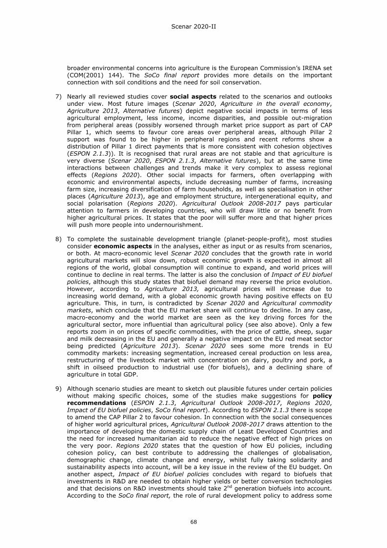
Scenar 2020-II

68

broader environmental concerns into agriculture is the European Commission’s IRENA set (COM(2001) 144). The SoCo final report provides more details on the important connection with soil conditions and the need for soil conservation.

7) Nearly all reviewed studies cover social aspects related to the scenarios and outlooks under view. Most future images (Scenar 2020, Agriculture in the overall economy, Agriculture 2013, Alternative futures) depict negative social impacts in terms of less agricultural employment, less income, income disparities, and possible out-migration from peripheral areas (possibly worsened through market price support as part of CAP Pillar 1, which seems to favour core areas over peripheral areas, although Pillar 2 support was found to be higher in peripheral regions and recent reforms show a distribution of Pillar 1 direct payments that is more consistent with cohesion objectives (ESPON 2.1.3)). It is recognised that rural areas are not stable and that agriculture is very diverse (Scenar 2020, ESPON 2.1.3, Alternative futures), but at the same time interactions between challenges and trends make it very complex to assess regional effects (Regions 2020). Other social impacts for farmers, often overlapping with economic and environmental aspects, include decreasing number of farms, increasing farm size, increasing diversification of farm households, as well as specialisation in other places (Agriculture 2013), age and employment structure, intergenerational equity, and social polarisation (Regions 2020). Agricultural Outlook 2008-2017 pays particular attention to farmers in developing countries, who will draw little or no benefit from higher agricultural prices. It states that the poor will suffer more and that higher prices will push more people into undernourishment.

8) To complete the sustainable development triangle (planet-people-profit), most studies consider economic aspects in the analyses, either as input or as results from scenarios, or both. At macro-economic level Scenar 2020 concludes that the growth rate in world agricultural markets will slow down, robust economic growth is expected in almost all regions of the world, global consumption will continue to expand, and world prices will continue to decline in real terms. The latter is also the conclusion of Impact of EU biofuel policies, although this study states that biofuel demand may reverse the price evolution. However, according to Agriculture 2013, agricultural prices will increase due to increasing world demand, with a global economic growth having positive effects on EU agriculture. This, in turn, is contradicted by Scenar 2020 and Agricultural commodity markets, which conclude that the EU market share will continue to decline. In any case, macro-economy and the world market are seen as the key driving forces for the agricultural sector, more influential than agricultural policy (see also above). Only a few reports zoom in on prices of specific commodities, with the price of cattle, sheep, sugar and milk decreasing in the EU and generally a negative impact on the EU red meat sector being predicted (Agriculture 2013). Scenar 2020 sees some more trends in EU commodity markets: increasing segmentation, increased cereal production on less area, restructuring of the livestock market with concentration on dairy, poultry and pork, a shift in oilseed production to industrial use (for biofuels), and a declining share of agriculture in total GDP.

9) Although scenario studies are meant to sketch out plausible futures under certain policies without making specific choices, some of the studies make suggestions for policy recommendations (ESPON 2.1.3, Agricultural Outlook 2008-2017, Regions 2020, Impact of EU biofuel policies, SoCo final report). According to ESPON 2.1.3 there is scope to amend the CAP Pillar 2 to favour cohesion. In connection with the social consequences of higher world agricultural prices, Agricultural Outlook 2008-2017 draws attention to the importance of developing the domestic supply chain of Least Developed Countries and the need for increased humanitarian aid to reduce the negative effect of high prices on the very poor. Regions 2020 states that the question of how EU policies, including cohesion policy, can best contribute to addressing the challenges of globalisation, demographic change, climate change and energy, whilst fully taking solidarity and sustainability aspects into account, will be a key issue in the review of the EU budget. On another aspect, Impact of EU biofuel policies concludes with regard to biofuels that investments in R&D are needed to obtain higher yields or better conversion technologies and that decisions on R&D investments should take 2nd generation biofuels into account. According to the SoCo final report, the role of rural development policy to address some

Scenar 2020-II

69

of the soil conservation needs and challenges should be continued into the future and conservation of agricultural soils is to become a rural development priority. Thus, the SoCo final report concludes that the Soil Framework Directive should be adopted and specific needs are formulated in relation to stakeholder involvement, standards, indicators, etc.

10) And finally, without making specific suggestions, it should be noted that many of the

studies make reference to the role of innovation and technological development with regard to the future of agriculture in Europe. This is referred to in relation to biofuel production (notably 2nd generation), productivity increase per unit land, or dealing with localised extreme events.

Scenar 2020-II

70

3. Refining the overall analysis – the agricultural sector

3.1. Introduction to the analysis of the agricultural sector The future of the agricultural sector in the European Union now seems set in a very different context than when originally investigated in the first Scenar 2020 study. Two major items are the increased volatility in agricultural commodity markets and the effect of mandated blending of biofuels. But in other respects the situation has not evolved much since a few years ago: an ageing farm population within the EU, an important wage differential between the agricultural and other economic sectors, the increasing productivity that is coming from investment in human and physical capital, and the role of land as a buffer among the factors of production. The interplay between all of these items is the subject of this updated analysis of the agricultural sector.

3.2. Economy-wide and global dynamics Worldwide differences in production and consumption growth can partly be explained by differences in economic and population growth between countries and country groups (Figure 3.1). Another important factor is that people do not eat much more if they get richer. Therefore, the so-called income elasticity is low and gets lower the richer people are. In general, the income elasticity is lower for crop than for livestock products. So if income increases, relatively more money is spent on meat products. Figure 3.1: World population, GDP, and GDP/cap annual growth rates (2007-2020).13 Source: United States Department of Agriculture/Economic Research Service Database (2009).

13 Note for the reader: Regional aggregations in the figures of the following sections are indicated as: • HighInc: Nafta (Canada, USA, Mexico), Oceania (mainly New Zealand and Australia), Japan and

South Korea. • C&SAmerica: Central and South America (including Brazil) and the Caribbean countries. • Africa: South Africa, all sub-Saharan countries and North Africa. • Asia: China, East Asia (including India) and Middle East. Not included in these figures: • Turkey. • Rest of Europe (Switzerland, Norway, Croatia and the other Western Balkan countries). • All countries belonging to the bloc of the former Soviet Union.

-1.00.01.02.03.04.05.06.07.0

EU-15 EU-10 EU-25 EU-02 HighInc C&SAmerica

Asia Africa

POP GDP GDP per capita

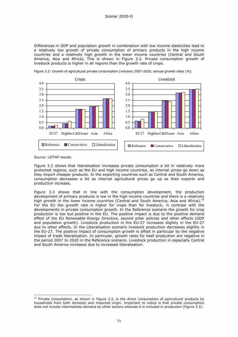
Scenar 2020-II

71

Differences in GDP and population growth in combination with low income elasticities lead to a relatively low growth of private consumption of primary products in the high income countries and a relatively high growth in the lower income countries (Central and South America, Asia and Africa). This is shown in Figure 3.2. Private consumption growth of livestock products is higher in all regions than the growth rate of crops. Figure 3.2: Growth of agricultural private consumption (volume) 2007-2020, annual growth rates (%).

Source: LEITAP results. Figure 3.2 shows that liberalisation increases private consumption a bit in relatively more protected regions, such as the EU and high income countries, as internal prices go down as they import cheaper products. In the exporting countries such as Central and South America, consumption decreases a bit as internal agricultural prices go up as their exports and production increase. Figure 3.3 shows that in line with the consumption development, the production development of primary products is low in the high income countries and there is a relatively high growth in the lower income countries (Central and South America, Asia and Africa).14 For the EU the growth rate is higher for crops than for livestock, in contrast with the developments in private consumption growth. In the Reference scenario the growth for crop production is low but positive in the EU. The positive impact is due to the positive demand effect of the EU Renewable Energy Directive, second pillar policies and other effects (GDP and population growth). Livestock production in the EU-27 increases slightly in the EU-27 due to other effects. In the Liberalisation scenario livestock production decreases slightly in the EU-27. The positive impact of consumption growth is offset in particular by the negative impact of trade liberalisation. In particular, growth rates for beef production are negative in the period 2007 to 2020 in the Reference scenario. Livestock production in especially Central and South America increases due to increased liberalisation.

14 Private consumption, as shown in Figure 3.2, is the direct consumption of agricultural products by households from both domestic and imported origin. Important to notice is that private consumption does not include intermediate demand by other sectors whereas it is included in production (Figure 3.3).

Crops Livestock

0.00.51.01.52.02.53.03.54.0

EU27 HighIncC&SAmer Asia Africa

Reference Conservative Liberalisation

0.00.51.01.52.02.53.03.54.0

EU27 HighIncC&SAmer Asia Africa

Reference Conservative Liberalisation

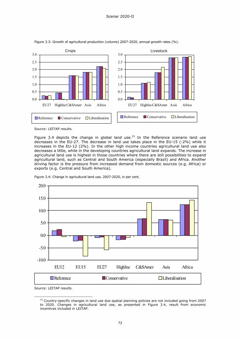
Scenar 2020-II

72

-10.0

-5.0

0.0

5.0

10.0

15.0

20.0

EU12 EU15 EU27 HighInc C&SAmer Asia Africa

Reference Conservative Liberalisation

Figure 3.3: Growth of agricultural production (volume) 2007-2020, annual growth rates (%).

Source: LEITAP results. Figure 3.4 depicts the change in global land use.15 In the Reference scenario land use decreases in the EU-27. The decrease in land use takes place in the EU-15 (-2%) while it increases in the EU-12 (2%). In the other high income countries agricultural land use also decreases a little, while in the developing countries agricultural land expands. The increase in agricultural land use is highest in those countries where there are still possibilities to expand agricultural land, such as Central and South America (especially Brazil) and Africa. Another driving factor is the pressure from increased demand from domestic sources (e.g. Africa) or exports (e.g. Central and South America). Figure 3.4: Change in agricultural land use, 2007-2020, in per cent.

Source: LEITAP results.

15 Country-specific changes in land use due spatial planning policies are not included going from 2007 to 2020. Changes in agricultural land use, as presented in Figure 3.4, result from economic incentives included in LEITAP.

0.0

0.5

1.0

1.5

2.0

2.5

3.0

EU27 HighIncC&SAmer Asia Africa

Reference Conservative Liberalisation

0.0

0.5

1.0

1.5

2.0

2.5

3.0

EU27 HighIncC&SAmer Asia Africa

Reference Conservative Liberalisation

Crops Livestock

Scenar 2020-II

73

The following figures present the results of the decomposition of the trade growth for crops (wheat, other grains, oilseeds, sugar, horticulture, other crops) livestock (primary and processed cattle, pork and poultry products) and agri-food products. Agri-food products present the total of primary and processed agricultural and food commodities, including crop and livestock products. (See Table 3.1.) To identify the separate impact of individual CAP, trade and biofuel policies on the scenario outcomes the total scenario impact has been decomposed into the following effects:16 • Total effect: Scenario outcome, includes all policy and other effects of the following sub-

items. • Border effect: Isolates the impact of changes in trade polices measures on the import

and export side. In the Reference and Conservative CAP scenario this is mainly the impact of the Falconer WTO proposal (including abolition of all export subsidies) and the bilateral trade agreements. In the Liberalisation scenario this is the total abolition of all export subsides and import tariffs.

• RenEnDir: Identifies the impact of the introduction of the mandatory blending

requirements of the EU Renewable Energy Directive. • Direct payments: Identifies the impact of changes in direct payments (first pillar). It is

the change in direct payments implemented under the Health Check reform and the scenario-specific assumptions up to 2020. The cuts in direct payments are 30%, 15% and 100% in respectively the Reference, Conservative CAP and Liberalisation scenarios.

• Rural development: Identifies the consequences of the transfer of additional funds to all

Pillar 2 measures under different scenarios. The increase in EAFRD payments are 105%, 45% and 100% in respectively the Reference, Conservative CAP and Liberalisation scenarios. The budgets are distributed across RD measures according to the current distribution in the RD plans.

• Other effects: Impact of change in population, production factor supply and productivity.

It is calculated as a separate scenario run. It is also mathematically equivalent to the difference between the total effect and the policy effects above, considered individually.

Figures 3.5 and 3.6 depict import and export growth in agri-food trade in the EU-27. Export growth of the EU in the Reference scenario is limited and mainly positive due to other effects (GDP and population growth) that lead to higher consumption in the world (see Figure 3.5). The other effects are higher for processed than for crops and livestock commodities as in general these products are demanded more as income grows (higher income elasticity of demand). The impact of the Falconer proposal is reflected in the impact of the border effect. The impact is negative for livestock and agri-food products. The latter is surprising as also the EU-27 gets enhanced access to other markets due to lower import barriers. However, this negative impact is mainly caused by the abolition of export subsidies, especially in the dairy sector. The impact of rural development spending is slightly positive on agri-food exports as especially human and physical capital investments improve productivity and therefore competiveness. The impact of the Renewable Energy Directive is negative as more biomass products are needed for domestic demand. Another factor is that the increased crop production inside the EU due to the Directive leads to higher production factor and therefore product prices inside the EU-27 relative to the prices in other countries. The impact of reducing direct payments is very small, indicating that direct payments are fairly decoupled. In the Liberalisation scenario (right-hand side of Figure 3.5) exports increase by 20% instead

16 Technically, the decomposition has been implemented by a sequence of consecutive scenario runs where each decomposed element has been added. This method gives only an indication or approximation of the size of the various impacts. This is because the size of the impacts is dependent on the order of the scenarios (path dependency). As the initial situation for the various scenarios is slightly different the height of the bars cannot be compared one-to-one across scenarios. Finally, cross or interaction effects are not separated out.

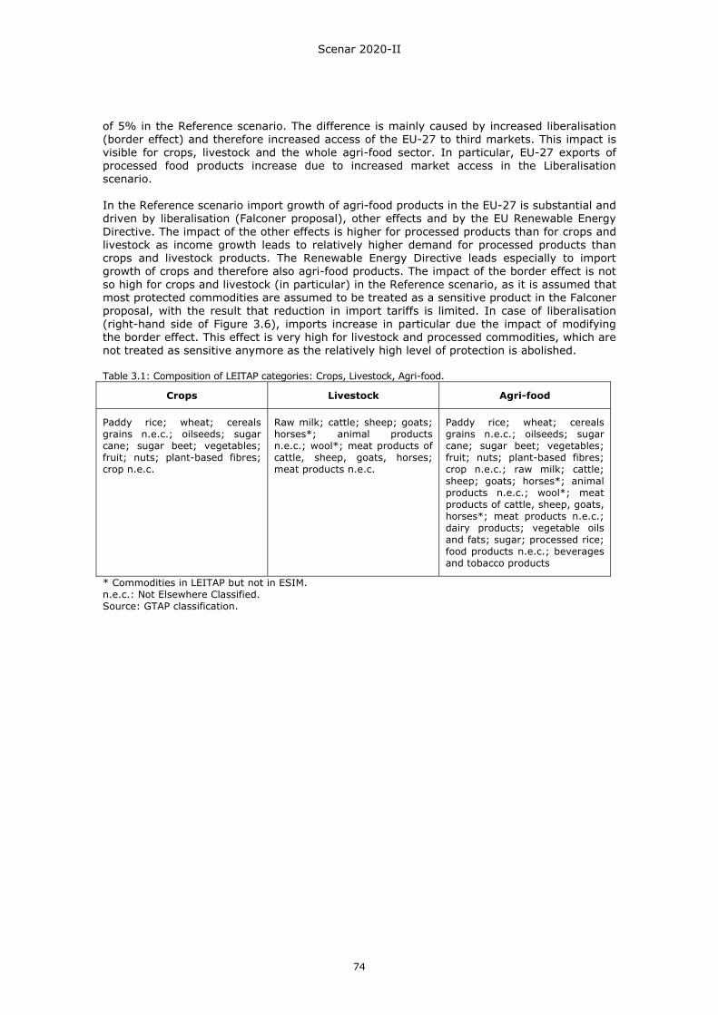
Scenar 2020-II

74

of 5% in the Reference scenario. The difference is mainly caused by increased liberalisation (border effect) and therefore increased access of the EU-27 to third markets. This impact is visible for crops, livestock and the whole agri-food sector. In particular, EU-27 exports of processed food products increase due to increased market access in the Liberalisation scenario. In the Reference scenario import growth of agri-food products in the EU-27 is substantial and driven by liberalisation (Falconer proposal), other effects and by the EU Renewable Energy Directive. The impact of the other effects is higher for processed products than for crops and livestock as income growth leads to relatively higher demand for processed products than crops and livestock products. The Renewable Energy Directive leads especially to import growth of crops and therefore also agri-food products. The impact of the border effect is not so high for crops and livestock (in particular) in the Reference scenario, as it is assumed that most protected commodities are assumed to be treated as a sensitive product in the Falconer proposal, with the result that reduction in import tariffs is limited. In case of liberalisation (right-hand side of Figure 3.6), imports increase in particular due the impact of modifying the border effect. This effect is very high for livestock and processed commodities, which are not treated as sensitive anymore as the relatively high level of protection is abolished. Table 3.1: Composition of LEITAP categories: Crops, Livestock, Agri-food.

Crops Livestock Agri-food

Paddy rice; wheat; cereals grains n.e.c.; oilseeds; sugar cane; sugar beet; vegetables; fruit; nuts; plant-based fibres; crop n.e.c.

Raw milk; cattle; sheep; goats; horses*; animal products n.e.c.; wool*; meat products of cattle, sheep, goats, horses; meat products n.e.c.

Paddy rice; wheat; cereals grains n.e.c.; oilseeds; sugar cane; sugar beet; vegetables; fruit; nuts; plant-based fibres; crop n.e.c.; raw milk; cattle; sheep; goats; horses*; animal products n.e.c.; wool*; meat products of cattle, sheep, goats, horses*; meat products n.e.c.; dairy products; vegetable oils and fats; sugar; processed rice; food products n.e.c.; beverages and tobacco products

* Commodities in LEITAP but not in ESIM. n.e.c.: Not Elsewhere Classified. Source: GTAP classification.

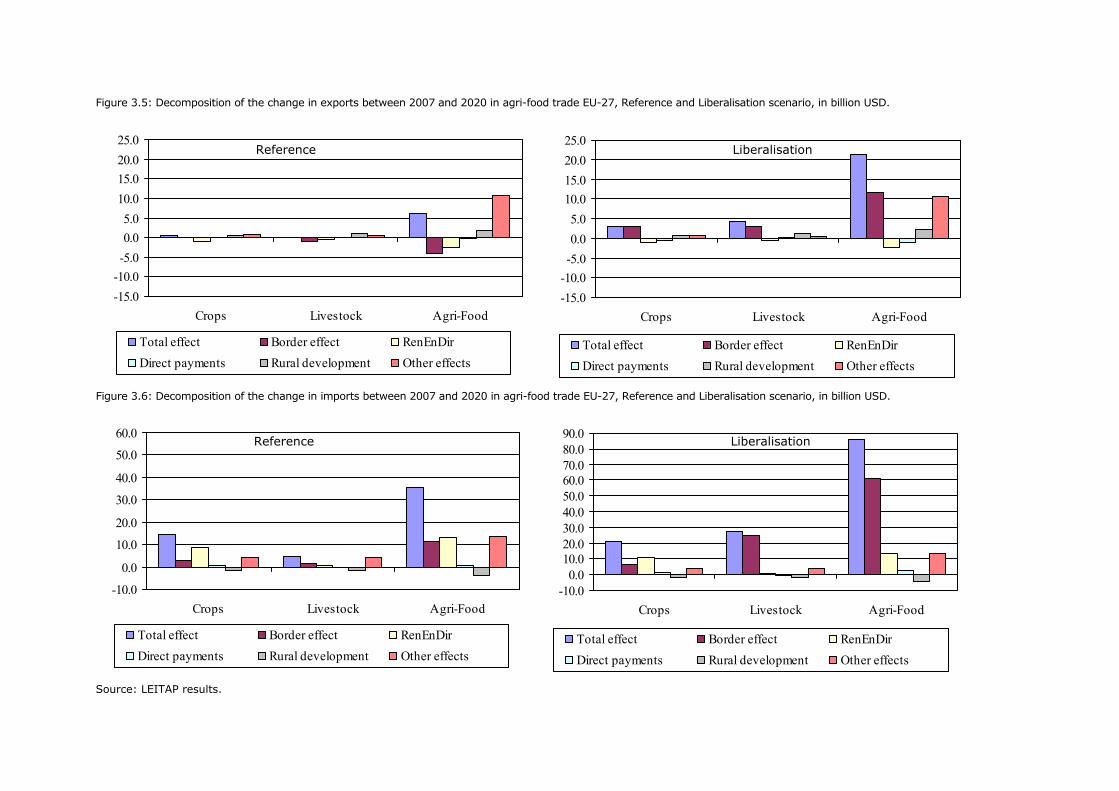
Figure 3.5: Decomposition of the change in exports between 2007 and 2020 in agri-food trade EU-27, Reference and Liberalisation scenario, in billion USD.

Figure 3.6: Decomposition of the change in imports between 2007 and 2020 in agri-food trade EU-27, Reference and Liberalisation scenario, in billion USD.

Source: LEITAP results.

-15.0-10.0-5.00.05.0

10.015.020.025.0

Crops Livestock Agri-Food

Total effect Border effect Biofuel directiveDirect payments Rural development Macro effects

-15.0-10.0-5.00.05.0

10.015.020.025.0

Crops Livestock Agri-Food

Total effect Border effect Biofuel directiveDirect payments Rural development Macro effects

Reference Liberalisation

-15.0-10.0-5.00.05.0

10.015.020.025.0

Crops Livestock Agri-Food

Total effect Border effect RenEnDirDirect payments Rural development Other effects

-15.0-10.0-5.00.05.0

10.015.020.025.0

Crops Livestock Agri-Food

Total effect Border effect RenEnDirDirect payments Rural development Other effects

Reference Liberalisation

-10.00.0

10.020.030.040.050.060.070.080.090.0

Crops Livestock Agri-Food

Total effect Border effect RenEnDirDirect payments Rural development Other effects

-10.0

0.0

10.0

20.0

30.0

40.0

50.0

60.0

Crops Livestock Agri-Food

Total effect Border effect RenEnDirDirect payments Rural development Other effects

Reference Liberalisation

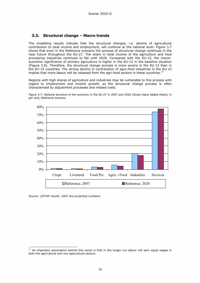
Scenar 2020-II

76

0%

10%

20%

30%

40%

50%

60%

70%

80%

Crops Livestock Food Prc. Agric.+Food Industries Services

Reference, 2007 Reference, 2020

3.3. Structural change – Macro trends The modelling results indicate that the structural changes, i.e. decline of agricultural contribution to total income and employment, will continue at the national level. Figure 3.7 shows that even in the Reference scenario the process of structural change continues in the near future throughout the EU-27. The share in total income of the agriculture and food processing industries continues to fall until 2020. Compared with the EU-15, the macro-economic significance of primary agriculture is higher in the EU-12 in the baseline situation (Figure 3.8). Therefore, the structural change process is more severe in the EU-12 than in the EU-15 countries. The strong decline in contribution of agro-food industries in the EU-12 implies that more labour will be released from the agri-food sectors in these countries.17 Regions with high shares of agriculture and industries may be vulnerable to this process with regard to employment and income growth, as the structural change process is often characterised by adjustment processes and related costs. Figure 3.7: Sectoral structure of the economy in the EU-27 in 2007 and 2020 (Gross Value Added share), in per cent, Reference scenario.

Source: LEITAP results. 2007 are projected numbers.

17 An important assumption behind this result is that in the longer run labour will earn equal wages in both the agricultural and non-agricultural sectors.

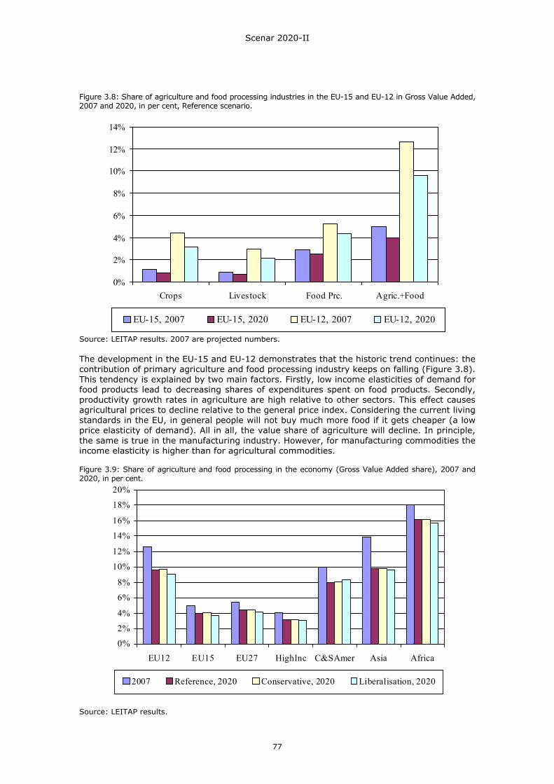
Scenar 2020-II

77

0%

2%

4%

6%

8%

10%

12%

14%

Crops Livestock Food Prc. Agric.+Food

EU-15, 2007 EU-15, 2020 EU-12, 2007 EU-12, 2020

0%

2%

4%

6%

8%

10%

12%

14%

16%

18%

20%

EU12 EU15 EU27 HighInc C&SAmer Asia Africa

2007 Reference, 2020 Conservative, 2020 Liberalisation, 2020

Figure 3.8: Share of agriculture and food processing industries in the EU-15 and EU-12 in Gross Value Added, 2007 and 2020, in per cent, Reference scenario. Source: LEITAP results. 2007 are projected numbers. The development in the EU-15 and EU-12 demonstrates that the historic trend continues: the contribution of primary agriculture and food processing industry keeps on falling (Figure 3.8). This tendency is explained by two main factors. Firstly, low income elasticities of demand for food products lead to decreasing shares of expenditures spent on food products. Secondly, productivity growth rates in agriculture are high relative to other sectors. This effect causes agricultural prices to decline relative to the general price index. Considering the current living standards in the EU, in general people will not buy much more food if it gets cheaper (a low price elasticity of demand). All in all, the value share of agriculture will decline. In principle, the same is true in the manufacturing industry. However, for manufacturing commodities the income elasticity is higher than for agricultural commodities. Figure 3.9: Share of agriculture and food processing in the economy (Gross Value Added share), 2007 and 2020, in per cent. Source: LEITAP results.

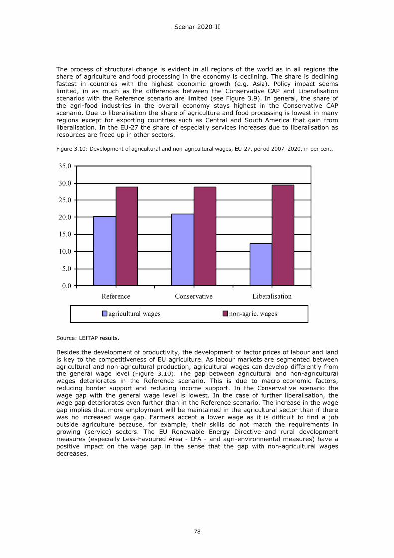
Scenar 2020-II

78

0.0

5.0

10.0

15.0

20.0

25.0

30.0

35.0

Reference Conservative Liberalisation

agricultural wages non-agric. wages

The process of structural change is evident in all regions of the world as in all regions the share of agriculture and food processing in the economy is declining. The share is declining fastest in countries with the highest economic growth (e.g. Asia). Policy impact seems limited, in as much as the differences between the Conservative CAP and Liberalisation scenarios with the Reference scenario are limited (see Figure 3.9). In general, the share of the agri-food industries in the overall economy stays highest in the Conservative CAP scenario. Due to liberalisation the share of agriculture and food processing is lowest in many regions except for exporting countries such as Central and South America that gain from liberalisation. In the EU-27 the share of especially services increases due to liberalisation as resources are freed up in other sectors. Figure 3.10: Development of agricultural and non-agricultural wages, EU-27, period 2007–2020, in per cent.

Source: LEITAP results. Besides the development of productivity, the development of factor prices of labour and land is key to the competitiveness of EU agriculture. As labour markets are segmented between agricultural and non-agricultural production, agricultural wages can develop differently from the general wage level (Figure 3.10). The gap between agricultural and non-agricultural wages deteriorates in the Reference scenario. This is due to macro-economic factors, reducing border support and reducing income support. In the Conservative scenario the wage gap with the general wage level is lowest. In the case of further liberalisation, the wage gap deteriorates even further than in the Reference scenario. The increase in the wage gap implies that more employment will be maintained in the agricultural sector than if there was no increased wage gap. Farmers accept a lower wage as it is difficult to find a job outside agriculture because, for example, their skills do not match the requirements in growing (service) sectors. The EU Renewable Energy Directive and rural development measures (especially Less-Favoured Area - LFA - and agri-environmental measures) have a positive impact on the wage gap in the sense that the gap with non-agricultural wages decreases.

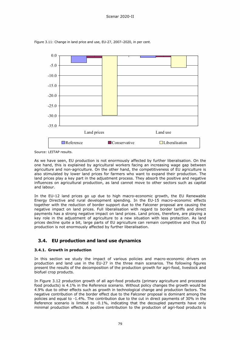
Scenar 2020-II

79

-35.0

-30.0

-25.0

-20.0

-15.0

-10.0

-5.0

0.0

Land prices Land use

Reference Conservative Liberalisation

Figure 3.11: Change in land price and use, EU-27, 2007–2020, in per cent. Source: LEITAP results. As we have seen, EU production is not enormously affected by further liberalisation. On the one hand, this is explained by agricultural workers facing an increasing wage gap between agriculture and non-agriculture. On the other hand, the competitiveness of EU agriculture is also stimulated by lower land prices for farmers who want to expand their production. The land prices play a key part in the adjustment process. They absorb the positive and negative influences on agricultural production, as land cannot move to other sectors such as capital and labour. In the EU-12 land prices go up due to high macro-economic growth, the EU Renewable Energy Directive and rural development spending. In the EU-15 macro-economic effects together with the reduction of border support due to the Falconer proposal are causing the negative impact on land prices. Full liberalisation with regard to border tariffs and direct payments has a strong negative impact on land prices. Land prices, therefore, are playing a key role in the adjustment of agriculture to a new situation with less protection. As land prices decline quite a bit, large parts of EU agriculture can remain competitive and thus EU production is not enormously affected by further liberalisation.

3.4. EU production and land use dynamics 3.4.1. Growth in production In this section we study the impact of various policies and macro-economic drivers on production and land use in the EU-27 in the three main scenarios. The following figures present the results of the decomposition of the production growth for agri-food, livestock and biofuel crop products. In Figure 3.12 production growth of all agri-food products (primary agriculture and processed food products) is 4.1% in the Reference scenario. Without policy changes the growth would be 4.9% due to other effects such as growth in technological change and production factors. The negative contribution of the border effect due to the Falconer proposal is dominant among the policies and equal to -1.4%. The contribution due to the cut in direct payments of 30% in the Reference scenario is limited to -0.1%, indicating that the decoupled payments have only minimal production effects. A positive contribution to the production of agri-food products is

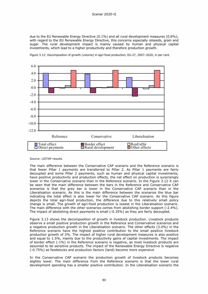
Scenar 2020-II

80

-12.0

-10.0

-8.0

-6.0

-4.0

-2.0

0.0

2.0

4.0

6.0

Reference Conservative Liberalisation

Total effect Border effect RenEnDirDirect payments Rural development Other effects

due to the EU Renewable Energy Directive (0.1%) and all rural development measures (0.6%); with regard to the EU Renewable Energy Directive, this concerns especially oilseeds, grain and sugar. The rural development impact is mainly caused by human and physical capital investments, which lead to a higher productivity and therefore production growth. Figure 3.12: Decomposition of growth (volume) in agri-food production, EU-27, 2007–2020, in per cent.

Source: LEITAP results. The main difference between the Conservative CAP scenario and the Reference scenario is that fewer Pillar 1 payments are transferred to Pillar 2. As Pillar 1 payments are fairly decoupled and some Pillar 2 payments, such as human and physical capital investments, have positive productivity and production effects, the net effect on production is surprisingly lower in the Conservative scenario than in the Reference scenario. In the Figure 3.12 it can be seen that the main difference between the bars in the Reference and Conservative CAP scenarios is that the grey bar is lower in the Conservative CAP scenario than in the Liberalisation scenario. As this is the main difference between the scenarios the blue bar indicating the total effect is also lower for the Conservative CAP scenario. As this figure depicts the total agri-food production, the difference due to this relatively small policy change is small. The growth of agri-food production is lowest in the Liberalisation scenario. The main difference with the other scenarios comes from abolishing border support (-2.4%). The impact of abolishing direct payments is small (-0.35%) as they are fairly decoupled. Figure 3.13 shows the decomposition of growth in livestock production. Livestock products observe a small positive production growth in the Reference and Conservative scenarios and a negative production growth in the Liberalisation scenario. The other effects (3.0%) in the Reference scenario have the highest positive contribution to the small positive livestock production growth of 2%. The impact of higher rural development measures is also positive and equal to 1.5%, mainly due to the productivity gains of capital investments. The impact of border effect (-1%) in the Reference scenario is negative, as most livestock products are assumed to be sensitive products. The impact of the Renewable Energy Directive is negative (-0.75%) as feedstocks and production factors (land) become more expensive In the Conservative CAP scenario the production growth of livestock products becomes slightly lower. The main difference from the Reference scenario is that the lower rural development spending has a smaller positive contribution. In the Liberalisation scenario the

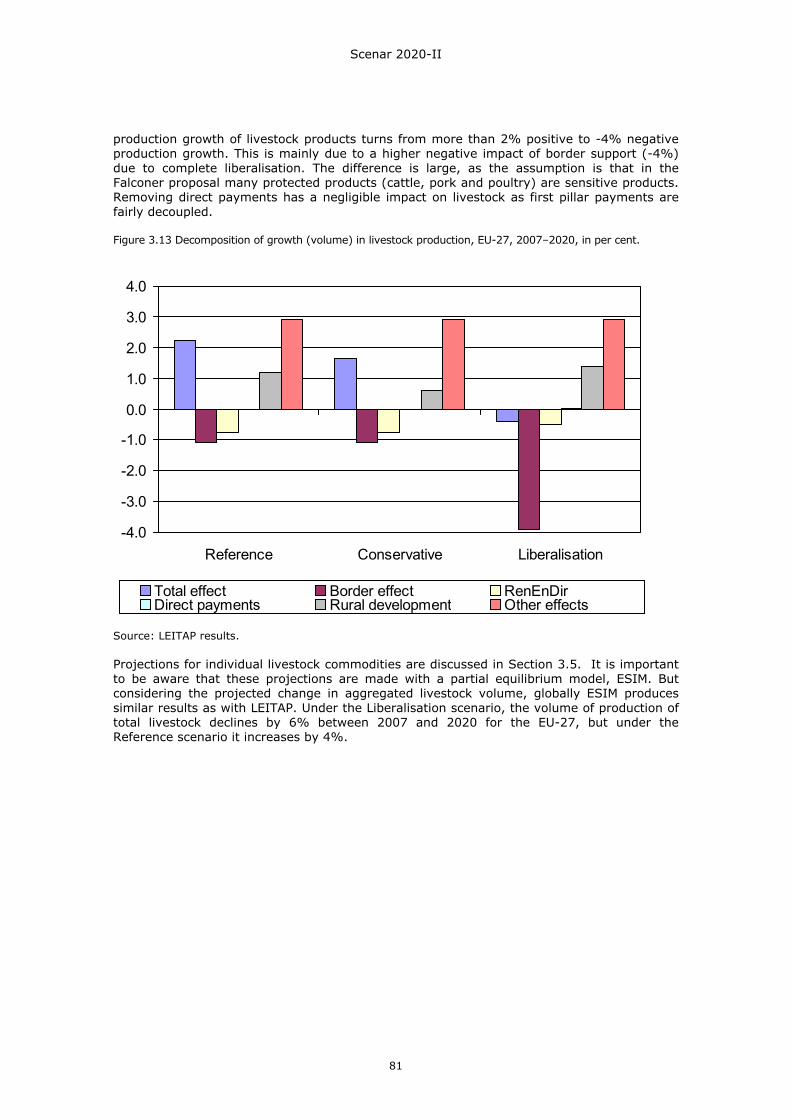
Scenar 2020-II

81

-4.0

-3.0

-2.0

-1.0

0.0

1.0

2.0

3.0

4.0

Reference Conservative Liberalisation

Total effect Border effect RenEnDirDirect payments Rural development Other effects

production growth of livestock products turns from more than 2% positive to -4% negative production growth. This is mainly due to a higher negative impact of border support (-4%) due to complete liberalisation. The difference is large, as the assumption is that in the Falconer proposal many protected products (cattle, pork and poultry) are sensitive products. Removing direct payments has a negligible impact on livestock as first pillar payments are fairly decoupled. Figure 3.13 Decomposition of growth (volume) in livestock production, EU-27, 2007–2020, in per cent.

Source: LEITAP results. Projections for individual livestock commodities are discussed in Section 3.5. It is important to be aware that these projections are made with a partial equilibrium model, ESIM. But considering the projected change in aggregated livestock volume, globally ESIM produces similar results as with LEITAP. Under the Liberalisation scenario, the volume of production of total livestock declines by 6% between 2007 and 2020 for the EU-27, but under the Reference scenario it increases by 4%.

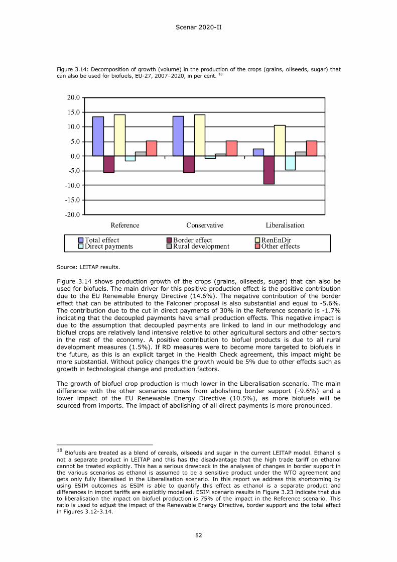
Scenar 2020-II

82

-20.0

-15.0

-10.0

-5.0

0.0

5.0

10.0

15.0

20.0

Reference Conservative Liberalisation

Total effect Border effect RenEnDirDirect payments Rural development Other effects

Figure 3.14: Decomposition of growth (volume) in the production of the crops (grains, oilseeds, sugar) that can also be used for biofuels, EU-27, 2007–2020, in per cent. 18

Source: LEITAP results. Figure 3.14 shows production growth of the crops (grains, oilseeds, sugar) that can also be used for biofuels. The main driver for this positive production effect is the positive contribution due to the EU Renewable Energy Directive (14.6%). The negative contribution of the border effect that can be attributed to the Falconer proposal is also substantial and equal to -5.6%. The contribution due to the cut in direct payments of 30% in the Reference scenario is -1.7% indicating that the decoupled payments have small production effects. This negative impact is due to the assumption that decoupled payments are linked to land in our methodology and biofuel crops are relatively land intensive relative to other agricultural sectors and other sectors in the rest of the economy. A positive contribution to biofuel products is due to all rural development measures (1.5%). If RD measures were to become more targeted to biofuels in the future, as this is an explicit target in the Health Check agreement, this impact might be more substantial. Without policy changes the growth would be 5% due to other effects such as growth in technological change and production factors. The growth of biofuel crop production is much lower in the Liberalisation scenario. The main difference with the other scenarios comes from abolishing border support (-9.6%) and a lower impact of the EU Renewable Energy Directive (10.5%), as more biofuels will be sourced from imports. The impact of abolishing of all direct payments is more pronounced.

18 Biofuels are treated as a blend of cereals, oilseeds and sugar in the current LEITAP model. Ethanol is not a separate product in LEITAP and this has the disadvantage that the high trade tariff on ethanol cannot be treated explicitly. This has a serious drawback in the analyses of changes in border support in the various scenarios as ethanol is assumed to be a sensitive product under the WTO agreement and gets only fully liberalised in the Liberalisation scenario. In this report we address this shortcoming by using ESIM outcomes as ESIM is able to quantify this effect as ethanol is a separate product and differences in import tariffs are explicitly modelled. ESIM scenario results in Figure 3.23 indicate that due to liberalisation the impact on biofuel production is 75% of the impact in the Reference scenario. This ratio is used to adjust the impact of the Renewable Energy Directive, border support and the total effect in Figures 3.12-3.14.

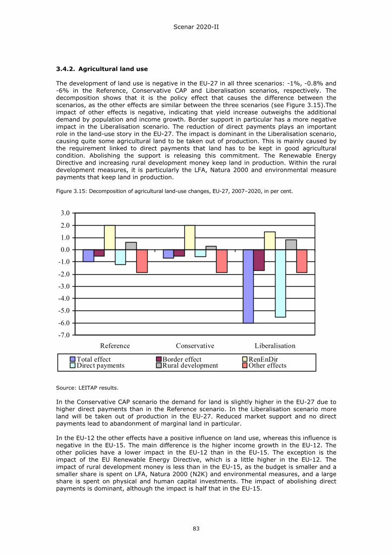
Scenar 2020-II

83

-7.0

-6.0

-5.0

-4.0

-3.0

-2.0

-1.0

0.0

1.0

2.0

3.0

Reference Conservative Liberalisation

Total effect Border effect RenEnDirDirect payments Rural development Other effects

3.4.2. Agricultural land use The development of land use is negative in the EU-27 in all three scenarios: -1%, -0.8% and -6% in the Reference, Conservative CAP and Liberalisation scenarios, respectively. The decomposition shows that it is the policy effect that causes the difference between the scenarios, as the other effects are similar between the three scenarios (see Figure 3.15).The impact of other effects is negative, indicating that yield increase outweighs the additional demand by population and income growth. Border support in particular has a more negative impact in the Liberalisation scenario. The reduction of direct payments plays an important role in the land-use story in the EU-27. The impact is dominant in the Liberalisation scenario, causing quite some agricultural land to be taken out of production. This is mainly caused by the requirement linked to direct payments that land has to be kept in good agricultural condition. Abolishing the support is releasing this commitment. The Renewable Energy Directive and increasing rural development money keep land in production. Within the rural development measures, it is particularly the LFA, Natura 2000 and environmental measure payments that keep land in production. Figure 3.15: Decomposition of agricultural land-use changes, EU-27, 2007–2020, in per cent.

Source: LEITAP results. In the Conservative CAP scenario the demand for land is slightly higher in the EU-27 due to higher direct payments than in the Reference scenario. In the Liberalisation scenario more land will be taken out of production in the EU-27. Reduced market support and no direct payments lead to abandonment of marginal land in particular. In the EU-12 the other effects have a positive influence on land use, whereas this influence is negative in the EU-15. The main difference is the higher income growth in the EU-12. The other policies have a lower impact in the EU-12 than in the EU-15. The exception is the impact of the EU Renewable Energy Directive, which is a little higher in the EU-12. The impact of rural development money is less than in the EU-15, as the budget is smaller and a smaller share is spent on LFA, Natura 2000 (N2K) and environmental measures, and a large share is spent on physical and human capital investments. The impact of abolishing direct payments is dominant, although the impact is half that in the EU-15.

Scenar 2020-II

84

3.5. Commodity markets 3.5.1. Price effects To explain the development of agriculture prospects at sectoral level, it is important to analyse the price changes at EU market level. The changes in real prices at producer level are presented in Table 3.2; the results are derived from ESIM. The results show an increase in prices of most arable crops used for biofuels (soybean, rapeseed and sunflower seed), with the exception of corn and sugar beets. The development of prices of sugar beets shows the effect of the EU sugar reform and the increased market liberalisation in the Reference scenario. The impact on the supported rice and barley markets is substantially negative due to market liberalisation (Falconer proposal). Real prices of livestock products decrease sharply in the Reference scenario. This is explained by the long-term trend and the market liberalisation in the Reference scenario. The latter especially affects prices of beef, sheep and milk and dairy products. Prices in the Liberalisation scenario decrease compared with the Reference scenario. Price changes range from more than -33% for beef, -18% for rice, -17% for sheep to about -1% for milk and eggs. The latter shows that there are sectors which are affected to a limited extent by liberalisation compared to other sectors. Compared to Nowicki et al. (2007), the decrease in cereal prices is rather large in the Liberalisation scenario. Model experiments show that this can be explained by the assumptions concerning the Renewable Energy Directive. Domestic ethanol production in the EU declines under liberalisation due to the strong cut in import tariffs under this scenario. This also affects prices of cereals in the Liberalisation scenario.

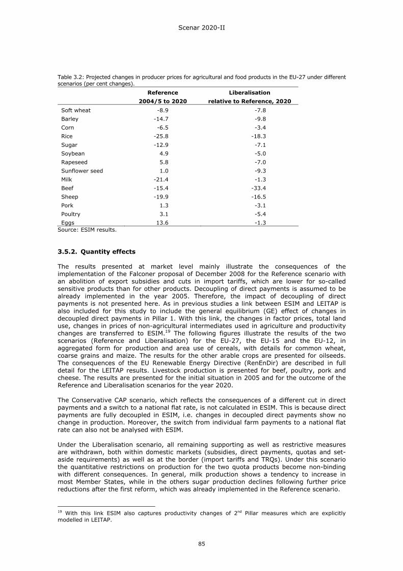
Scenar 2020-II

85

Table 3.2: Projected changes in producer prices for agricultural and food products in the EU-27 under different scenarios (per cent changes).

Reference Liberalisation 2004/5 to 2020 relative to Reference, 2020

Soft wheat -8.9 -7.8 Barley -14.7 -9.8 Corn -6.5 -3.4 Rice -25.8 -18.3 Sugar -12.9 -7.1 Soybean 4.9 -5.0 Rapeseed 5.8 -7.0 Sunflower seed 1.0 -9.3 Milk -21.4 -1.3 Beef -15.4 -33.4 Sheep -19.9 -16.5 Pork 1.3 -3.1 Poultry 3.1 -5.4 Eggs 13.6 -1.3

Source: ESIM results. 3.5.2. Quantity effects The results presented at market level mainly illustrate the consequences of the implementation of the Falconer proposal of December 2008 for the Reference scenario with an abolition of export subsidies and cuts in import tariffs, which are lower for so-called sensitive products than for other products. Decoupling of direct payments is assumed to be already implemented in the year 2005. Therefore, the impact of decoupling of direct payments is not presented here. As in previous studies a link between ESIM and LEITAP is also included for this study to include the general equilibrium (GE) effect of changes in decoupled direct payments in Pillar 1. With this link, the changes in factor prices, total land use, changes in prices of non-agricultural intermediates used in agriculture and productivity changes are transferred to ESIM.19 The following figures illustrate the results of the two scenarios (Reference and Liberalisation) for the EU-27, the EU-15 and the EU-12, in aggregated form for production and area use of cereals, with details for common wheat, coarse grains and maize. The results for the other arable crops are presented for oilseeds. The consequences of the EU Renewable Energy Directive (RenEnDir) are described in full detail for the LEITAP results. Livestock production is presented for beef, poultry, pork and cheese. The results are presented for the initial situation in 2005 and for the outcome of the Reference and Liberalisation scenarios for the year 2020. The Conservative CAP scenario, which reflects the consequences of a different cut in direct payments and a switch to a national flat rate, is not calculated in ESIM. This is because direct payments are fully decoupled in ESIM, i.e. changes in decoupled direct payments show no change in production. Moreover, the switch from individual farm payments to a national flat rate can also not be analysed with ESIM. Under the Liberalisation scenario, all remaining supporting as well as restrictive measures are withdrawn, both within domestic markets (subsidies, direct payments, quotas and set-aside requirements) as well as at the border (import tariffs and TRQs). Under this scenario the quantitative restrictions on production for the two quota products become non-binding with different consequences. In general, milk production shows a tendency to increase in most Member States, while in the others sugar production declines following further price reductions after the first reform, which was already implemented in the Reference scenario. 19 With this link ESIM also captures productivity changes of 2nd Pillar measures which are explicitly modelled in LEITAP.

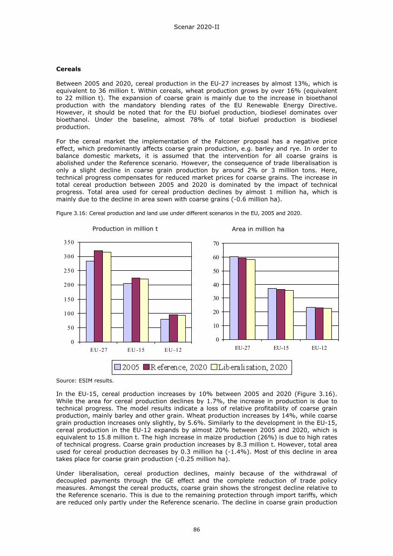
Scenar 2020-II

86

Cereals Between 2005 and 2020, cereal production in the EU-27 increases by almost 13%, which is equivalent to 36 million t. Within cereals, wheat production grows by over 16% (equivalent to 22 million t). The expansion of coarse grain is mainly due to the increase in bioethanol production with the mandatory blending rates of the EU Renewable Energy Directive. However, it should be noted that for the EU biofuel production, biodiesel dominates over bioethanol. Under the baseline, almost 78% of total biofuel production is biodiesel production. For the cereal market the implementation of the Falconer proposal has a negative price effect, which predominantly affects coarse grain production, e.g. barley and rye. In order to balance domestic markets, it is assumed that the intervention for all coarse grains is abolished under the Reference scenario. However, the consequence of trade liberalisation is only a slight decline in coarse grain production by around 2% or 3 million tons. Here, technical progress compensates for reduced market prices for coarse grains. The increase in total cereal production between 2005 and 2020 is dominated by the impact of technical progress. Total area used for cereal production declines by almost 1 million ha, which is mainly due to the decline in area sown with coarse grains (-0.6 million ha). Figure 3.16: Cereal production and land use under different scenarios in the EU, 2005 and 2020.

Source: ESIM results. In the EU-15, cereal production increases by 10% between 2005 and 2020 (Figure 3.16). While the area for cereal production declines by 1.7%, the increase in production is due to technical progress. The model results indicate a loss of relative profitability of coarse grain production, mainly barley and other grain. Wheat production increases by 14%, while coarse grain production increases only slightly, by 5.6%. Similarly to the development in the EU-15, cereal production in the EU-12 expands by almost 20% between 2005 and 2020, which is equivalent to 15.8 million t. The high increase in maize production (26%) is due to high rates of technical progress. Coarse grain production increases by 8.3 million t. However, total area used for cereal production decreases by 0.3 million ha (-1.4%). Most of this decline in area takes place for coarse grain production (-0.25 million ha). Under liberalisation, cereal production declines, mainly because of the withdrawal of decoupled payments through the GE effect and the complete reduction of trade policy measures. Amongst the cereal products, coarse grain shows the strongest decline relative to the Reference scenario. This is due to the remaining protection through import tariffs, which are reduced only partly under the Reference scenario. The decline in coarse grain production

0

50

100

150

200

250

300

350

EU -27 EU -15 EU -12

Production in million t Area in million ha

0

10

20

30

40

50

60

70

EU-27 EU-15 EU-12

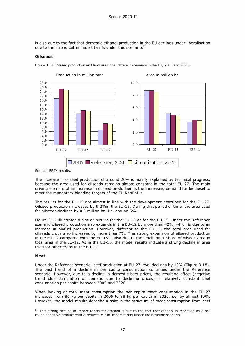
Scenar 2020-II

87

is also due to the fact that domestic ethanol production in the EU declines under liberalisation due to the strong cut in import tariffs under this scenario.20 Oilseeds Figure 3.17: Oilseed production and land use under different scenarios in the EU, 2005 and 2020.

Source: ESIM results. The increase in oilseed production of around 20% is mainly explained by technical progress, because the area used for oilseeds remains almost constant in the total EU-27. The main driving element of an increase in oilseed production is the increasing demand for biodiesel to meet the mandatory blending targets of the EU RenEnDir. The results for the EU-15 are almost in line with the development described for the EU-27. Oilseed production increases by 9.2%in the EU-15. During that period of time, the area used for oilseeds declines by 0.3 million ha, i.e. around 5%. Figure 3.17 illustrates a similar picture for the EU-12 as for the EU-15. Under the Reference scenario oilseed production also expands in the EU-12 by more than 42%, which is due to an increase in biofuel production. However, different to the EU-15, the total area used for oilseeds crops also increases by more than 7%. The strong expansion of oilseed production in the EU-12 compared with the EU-15 is also due to the small initial share of oilseed area in total area in the EU-12. As in the EU-15, the model results indicate a strong decline in area used for other crops in the EU-12. Meat Under the Reference scenario, beef production at EU-27 level declines by 10% (Figure 3.18). The past trend of a decline in per capita consumption continues under the Reference scenario. However, due to a decline in domestic beef prices, the resulting effect (negative trend plus stimulation of demand due to declining prices) is relatively constant beef consumption per capita between 2005 and 2020. When looking at total meat consumption the per capita meat consumption in the EU-27 increases from 80 kg per capita in 2005 to 88 kg per capita in 2020, i.e. by almost 10%. However, the model results describe a shift in the structure of meat consumption from beef 20 This strong decline in import tariffs for ethanol is due to the fact that ethanol is modelled as a so-called sensitive product with a reduced cut in import tariffs under the baseline scenario.

0.02.04.06.08.0

10.012.014.016.018.020.022.024.026.028.0

EU-27 EU-15 EU-12

Area in million ha

0.0

2.0

4.0

6.0

8.0

10.0

EU-27 EU-15 EU-12

Production in million tons

Scenar 2020-II

88

meat to pork and poultry meat.21 In 2005, the share of red meat in total meat consumption per capita was 21% and 18% in 2020, respectively. Figure 3.18: Production and consumption of beef under the different scenarios in the EU, 2005 and 2020.

Source: ESIM results. The general trends in the livestock market in the EU-15 are similar to those at EU-27 level. Due to (partial) trade liberalisation, EU-15 beef production declines between 2005 and 2020 by 10%, i.e. 0.8 million t. Here, the negative trend in beef consumption is stronger than the positive impact of declining prices. On the consumption side, total meat consumption per capita increases by almost 2.5% in the EU-15; but the share of beef decreases relative to pork and poultry, which is consistent with an observed shift in consumer preference. Under full liberalisation, declining prices lead to a strong decline in beef production in all EU Member States. Total beef production declines by more than 30%. Under liberalisation lower beef prices stimulate the demand in beef consumption, and per capita demand for beef is projected to be 10% higher in 2020 relative to the consumption level under the Reference scenario. In ESIM, beef production (liveweight and carcasses) is modelled as an independent activity which is not fully coupled to milk production. There is a positive cross-price elasticity between beef and milk production, but the own price elasticity of beef production still dominates the supply response. Therefore, the strong supply response under liberalisation shows the response of specialised beef production and not the supply response of beef production in terms of slaughtered dairy cows, which is fully coupled to milk production.22 While production for beef is projected to decline, the production of other livestock production increases under the Reference scenario (Figure 3.19 to Figure 3.21). EU-27 poultry meat and cheese production increase strongly by 13% for poultry and by more than 22% for cheese, 21 The difference among products is mainly due to different levels in income elasticities and partly the result of a consumer preference shift from beef to pork and poultry, which varies according to the scenario. Income elasticities are rather high for pork and poultry while income elasticities for beef are rather low. In ESIM there is also an autonomous trend in demand, apart from the endogenous impact of income and price changes; here the shifters for pork and poultry are positive, while beef has a small negative shifter that also contributes to this change. With these shifters we mimic the changes in preference. 22 Comparing the production decline for beef calculated by ESIM with changes indicated by LEITAP, there is a stronger response for ESIM. In LEITAP beef production is projected to change by -14%. The main reason is the difference in the composition of beef: in ESIM, this includes only liveweight and carcasses, whereas in LEITAP this includes all processed and liveweight beef sales. In addition, LEITAP, as a general equilibrium model, adjusts all factors of production in all sectors of the economy, which dampens the change in beef production in LEITAP.

0

1

2

3

4

5

6

7

8

9

E U -27 E U -15 E U -120

5

10

15

20

25

E U -27 E U -15 E U -12

Production in million tons Consumption in kg per capita

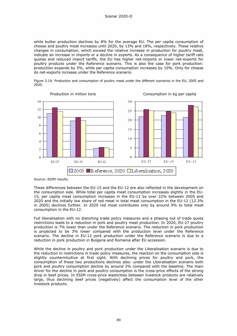
Scenar 2020-II

89

while butter production declines by 8% for the average EU. The per capita consumption of cheese and poultry meat increases until 2020, by 13% and 18%, respectively. These relative changes in consumption, which exceed the relative increase in production for poultry meat, indicate an increase in imports or a decline in exports. As a consequence of higher tariff rate quotas and reduced import tariffs, the EU has higher net-imports or lower net-exports for poultry products under the Reference scenario. This is also the case for pork production: production expands by 5%, while per capita consumption increases by 10%. Only for cheese do net-exports increase under the Reference scenario. Figure 3.19: Production and consumption of poultry meat under the different scenarios in the EU, 2005 and 2020.

Source: ESIM results. These differences between the EU-15 and the EU-12 are also reflected in the development on the consumption side. While total per capita meat consumption increases slightly in the EU-15, per capita meat consumption increases in the EU-12 by over 22% between 2005 and 2020 and the initially low share of red meat in total meat consumption in the EU-12 (12.3% in 2005) declines further. In 2020 red meat contributes only by around 9% to total meat consumption in the EU-12. Full liberalisation with no distorting trade policy measures and a phasing out of trade quota restrictions leads to a reduction in pork and poultry meat production. In 2020, EU-27 poultry production is 7% lower than under the Reference scenario. The reduction in pork production is projected to be 3% lower compared with the production level under the Reference scenario. The decline in EU-12 pork production under the Reference scenario is due to a reduction in pork production in Bulgaria and Romania after EU accession. While the decline in poultry and pork production under the Liberalisation scenario is due to the reduction in restrictions in trade policy measures, the reaction on the consumption side is slightly counterintuitive at first sight. With declining prices for poultry and pork, the consumption of these two productions declines also: under the Liberalisation scenario both pork and poultry consumption decline by around 3% compared with the baseline. The main driver for the decline in pork and poultry consumption is the cross-price effects of the strong drop in beef prices. In ESIM cross-price elasticities between livestock products are relatively large, thus declining beef prices (negatively) affect the consumption level of the other livestock products.

0

2

4

6

8

10

12

14

EU-27 EU-15 EU-120

5

1 0

1 5

2 0

2 5

3 0

E U -27 E U -15 E U -12

Production in million tons Consumption in kg per capita

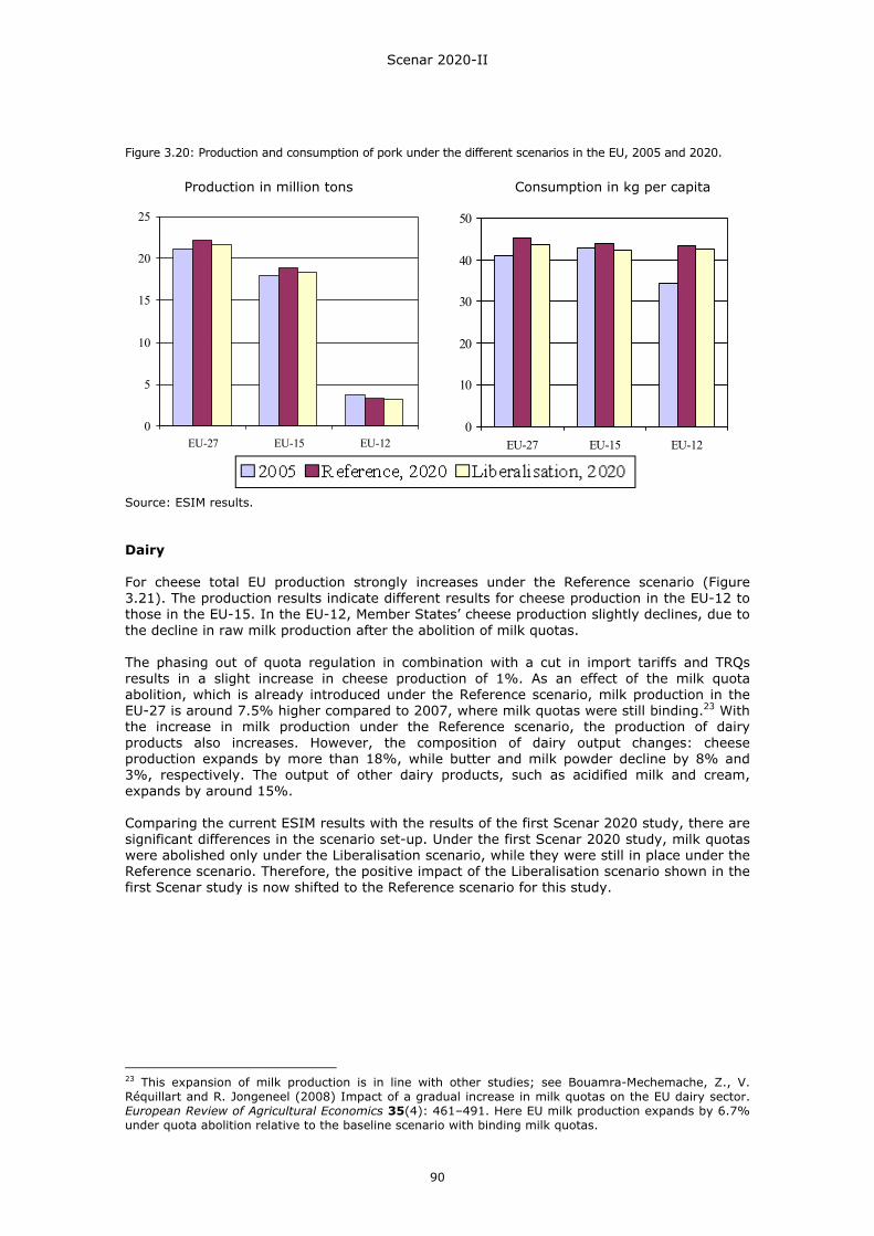
Scenar 2020-II

90

Figure 3.20: Production and consumption of pork under the different scenarios in the EU, 2005 and 2020.

Source: ESIM results. Dairy For cheese total EU production strongly increases under the Reference scenario (Figure 3.21). The production results indicate different results for cheese production in the EU-12 to those in the EU-15. In the EU-12, Member States’ cheese production slightly declines, due to the decline in raw milk production after the abolition of milk quotas. The phasing out of quota regulation in combination with a cut in import tariffs and TRQs results in a slight increase in cheese production of 1%. As an effect of the milk quota abolition, which is already introduced under the Reference scenario, milk production in the EU-27 is around 7.5% higher compared to 2007, where milk quotas were still binding.23 With the increase in milk production under the Reference scenario, the production of dairy products also increases. However, the composition of dairy output changes: cheese production expands by more than 18%, while butter and milk powder decline by 8% and 3%, respectively. The output of other dairy products, such as acidified milk and cream, expands by around 15%. Comparing the current ESIM results with the results of the first Scenar 2020 study, there are significant differences in the scenario set-up. Under the first Scenar 2020 study, milk quotas were abolished only under the Liberalisation scenario, while they were still in place under the Reference scenario. Therefore, the positive impact of the Liberalisation scenario shown in the first Scenar study is now shifted to the Reference scenario for this study.

23 This expansion of milk production is in line with other studies; see Bouamra-Mechemache, Z., V. Réquillart and R. Jongeneel (2008) Impact of a gradual increase in milk quotas on the EU dairy sector. European Review of Agricultural Economics 35(4): 461–491. Here EU milk production expands by 6.7% under quota abolition relative to the baseline scenario with binding milk quotas.

0

5

10

15

20

25

EU-27 EU-15 EU-120

10

20

30

40

50

EU-27 EU-15 EU-12

Production in million tons Consumption in kg per capita

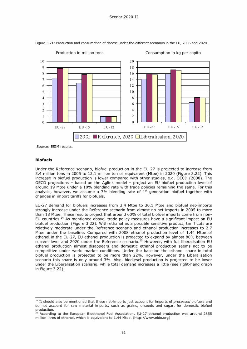
Scenar 2020-II

91

Figure 3.21: Production and consumption of cheese under the different scenarios in the EU, 2005 and 2020.

Source: ESIM results. Biofuels Under the Reference scenario, biofuel production in the EU-27 is projected to increase from 3.4 million tons in 2005 to 12.1 million ton oil equivalent (Mtoe) in 2020 (Figure 3.22). This increase in biofuel production is lower compared with other studies, e.g. OECD (2008). The OECD projections – based on the Aglink model – project an EU biofuel production level of around 19 Mtoe under a 10% blending rate with trade policies remaining the same. For this analysis, however, we assume a 7% blending rate of 1st generation biofuel together with changes in import tariffs for biofuels. EU-27 demand for biofuels increases from 3.4 Mtoe to 30.1 Mtoe and biofuel net-imports strongly increase under the Reference scenario from almost no net-imports in 2005 to more than 18 Mtoe. These results project that around 60% of total biofuel imports come from non-EU countries.24 As mentioned above, trade policy measures have a significant impact on EU biofuel production (Figure 3.22). With ethanol as a possible sensitive product, tariff cuts are relatively moderate under the Reference scenario and ethanol production increases to 2.7 Mtoe under the baseline. Compared with 2008 ethanol production level of 1.44 Mtoe of ethanol in the EU-27, EU ethanol production is projected to expand by almost 80% between current level and 2020 under the Reference scenario.25 However, with full liberalisation EU ethanol production almost disappears and domestic ethanol production seems not to be competitive under world market conditions. Under the baseline the ethanol share in total biofuel production is projected to be more than 22%. However, under the Liberalisation scenario this share is only around 3%. Also, biodiesel production is projected to be lower under the Liberalisation scenario, while total demand increases a little (see right-hand graph in Figure 3.22).

24 It should also be mentioned that these net-imports just account for imports of processed biofuels and do not account for raw material imports, such as grains, oilseeds and sugar, for domestic biofuel production. 25 According to the European Bioethanol Fuel Association, EU-27 ethanol production was around 2855 million litres of ethanol, which is equivalent to 1.44 Mtoe. (http://www.ebio.org)

0

12

3

45

6

7

89

10

E U -27 EU -15 EU -120

24

68

10

1214

1618

20

EU -27 EU -15 EU -12

Production in million tons Consumption in kg per capita

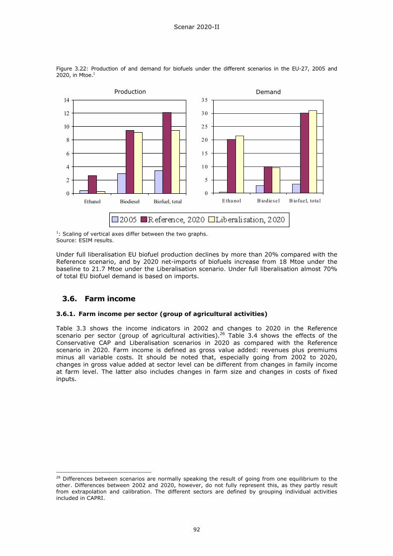
Scenar 2020-II

92

Figure 3.22: Production of and demand for biofuels under the different scenarios in the EU-27, 2005 and 2020, in Mtoe.1

1: Scaling of vertical axes differ between the two graphs. Source: ESIM results. Under full liberalisation EU biofuel production declines by more than 20% compared with the Reference scenario, and by 2020 net-imports of biofuels increase from 18 Mtoe under the baseline to 21.7 Mtoe under the Liberalisation scenario. Under full liberalisation almost 70% of total EU biofuel demand is based on imports.

3.6. Farm income 3.6.1. Farm income per sector (group of agricultural activities) Table 3.3 shows the income indicators in 2002 and changes to 2020 in the Reference scenario per sector (group of agricultural activities).26 Table 3.4 shows the effects of the Conservative CAP and Liberalisation scenarios in 2020 as compared with the Reference scenario in 2020. Farm income is defined as gross value added: revenues plus premiums minus all variable costs. It should be noted that, especially going from 2002 to 2020, changes in gross value added at sector level can be different from changes in family income at farm level. The latter also includes changes in farm size and changes in costs of fixed inputs.

26 Differences between scenarios are normally speaking the result of going from one equilibrium to the other. Differences between 2002 and 2020, however, do not fully represent this, as they partly result from extrapolation and calibration. The different sectors are defined by grouping individual activities included in CAPRI.

0

5

10

15

20

25

30

35

Ethanol B iodiese l B iofue l, tota l

Production Demand

0

2

4

6

8

10

12

14

Ethanol Biodiesel Biofuel, total

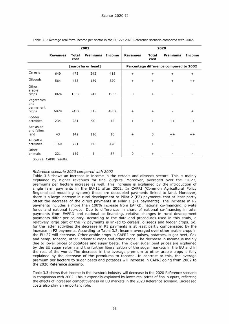
Scenar 2020-II

93

Table 3.3: Average real farm income per sector in the EU-27: 2020 Reference scenario compared with 2002.

2002 2020

Revenues Total cost

Premiums Income Revenues Total cost

Premiums Income

[euro/ha or head] Percentage difference compared to 2002

Cereals 649 473 242 418 + + + +

Oilseeds 564 433 189 320 + + + ++

Other arable crops 3024 1332 242 1933 0 + - -

Vegetables and permanent crops 6979 2432 315 4862 + + - +

Fodder activities 234 281 90 42 + + ++ ++

Set-aside and fallow land 43 142 116 16 + 0 ++ ++

All cattle activities 1140 721 60 478 - + - -

Other animals 221 139 5 87 0 + - -

Source: CAPRI results. Reference scenario 2020 compared with 2002 Table 3.3 shows an increase in income in the cereals and oilseeds sectors. This is mainly explained by higher revenues for final outputs. Moreover, averaged over the EU-27, premiums per hectare increase as well. This increase is explained by the introduction of single farm payments in the EU-12 after 2002. In CAPRI (Common Agricultural Policy Regionalised modelling system) these are decoupled payments linked to land. Moreover, there is a large increase in rural development or Pillar 2 (P2) payments, that at least partly offset the decrease of the direct payments in Pillar 1 (P1 payments). The increase in P2 payments includes a more than 100% increase from EAFRD, national co-financing, private funds and national top-ups. Due to differences in share of national co-financing in total payments from EAFRD and national co-financing, relative changes in rural development payments differ per country. According to the data and procedures used in this study, a relatively large part of the P2 payments is linked to cereals, oilseeds and fodder crops. So, for the latter activities the decrease in P1 payments is at least partly compensated by the increase in P2 payments. According to Table 3.3, income averaged over other arable crops in the EU-27 will decrease. Other arable crops in CAPRI are pulses, potatoes, sugar beet, flax and hemp, tobacco, other industrial crops and other crops. The decrease in income is mainly due to lower prices of potatoes and sugar beets. The lower sugar beet prices are explained by the EU sugar reform and the further liberalisation of the sugar markets in the EU and in the rest of the world. The decrease in the average premium to other arable crops is fully explained by the decrease of the premiums to tobacco. In contrast to this, the average premium per hectare to sugar beets and potatoes will increase in CAPRI going from 2002 to the 2020 Reference scenario. Table 3.3 shows that income in the livestock industry will decrease in the 2020 Reference scenario in comparison with 2002. This is especially explained by lower real prices of final outputs, reflecting the effects of increased competitiveness on EU markets in the 2020 Reference scenario. Increased costs also play an important role.

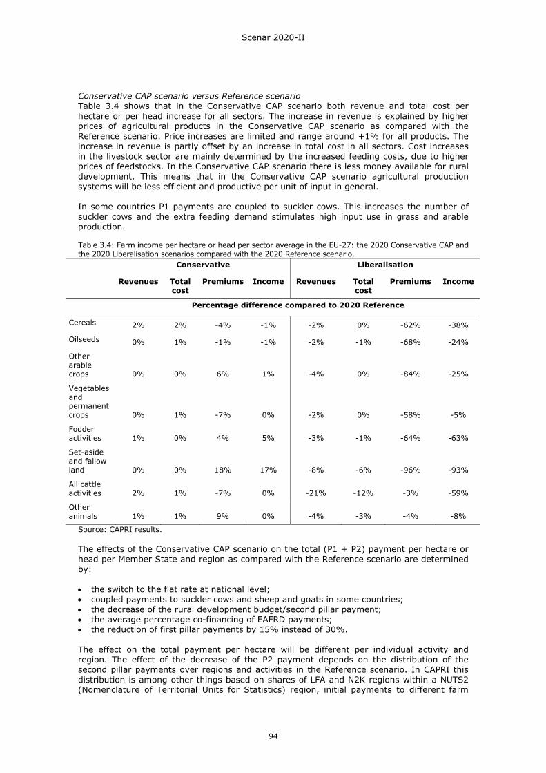
Scenar 2020-II

94

Conservative CAP scenario versus Reference scenario Table 3.4 shows that in the Conservative CAP scenario both revenue and total cost per hectare or per head increase for all sectors. The increase in revenue is explained by higher prices of agricultural products in the Conservative CAP scenario as compared with the Reference scenario. Price increases are limited and range around +1% for all products. The increase in revenue is partly offset by an increase in total cost in all sectors. Cost increases in the livestock sector are mainly determined by the increased feeding costs, due to higher prices of feedstocks. In the Conservative CAP scenario there is less money available for rural development. This means that in the Conservative CAP scenario agricultural production systems will be less efficient and productive per unit of input in general. In some countries P1 payments are coupled to suckler cows. This increases the number of suckler cows and the extra feeding demand stimulates high input use in grass and arable production. Table 3.4: Farm income per hectare or head per sector average in the EU-27: the 2020 Conservative CAP and the 2020 Liberalisation scenarios compared with the 2020 Reference scenario.

Conservative Liberalisation

Revenues Total cost

Premiums Income Revenues Total cost

Premiums Income

Percentage difference compared to 2020 Reference

Cereals 2% 2% -4% -1% -2% 0% -62% -38%

Oilseeds 0% 1% -1% -1% -2% -1% -68% -24%

Other arable crops 0% 0% 6% 1% -4% 0% -84% -25%

Vegetables and permanent crops 0% 1% -7% 0% -2% 0% -58% -5%

Fodder activities 1% 0% 4% 5% -3% -1% -64% -63%

Set-aside and fallow land 0% 0% 18% 17% -8% -6% -96% -93%

All cattle activities 2% 1% -7% 0% -21% -12% -3% -59%

Other animals 1% 1% 9% 0% -4% -3% -4% -8%

Source: CAPRI results. The effects of the Conservative CAP scenario on the total (P1 + P2) payment per hectare or head per Member State and region as compared with the Reference scenario are determined by: • the switch to the flat rate at national level; • coupled payments to suckler cows and sheep and goats in some countries; • the decrease of the rural development budget/second pillar payment; • the average percentage co-financing of EAFRD payments; • the reduction of first pillar payments by 15% instead of 30%. The effect on the total payment per hectare will be different per individual activity and region. The effect of the decrease of the P2 payment depends on the distribution of the second pillar payments over regions and activities in the Reference scenario. In CAPRI this distribution is among other things based on shares of LFA and N2K regions within a NUTS2 (Nomenclature of Territorial Units for Statistics) region, initial payments to different farm

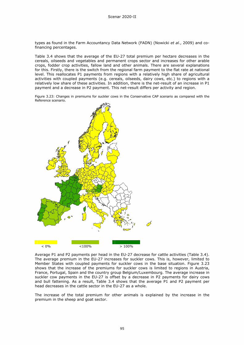
Scenar 2020-II

95

types as found in the Farm Accountancy Data Network (FADN) (Nowicki et al., 2009) and co-financing percentages. Table 3.4 shows that the average of the EU-27 total premium per hectare decreases in the cereals, oilseeds and vegetables and permanent crops sector and increases for other arable crops, fodder crop activities, fallow land and other animals. There are several explanations for this. Firstly, there is the switch from the regional farm payment to the flat rate at national level. This reallocates P1 payments from regions with a relatively high share of agricultural activities with coupled payments (e.g. cereals, oilseeds, dairy cows, etc.) to regions with a relatively low share of these activities. In addition, there is the net-result of an increase in P1 payment and a decrease in P2 payment. This net-result differs per activity and region. Figure 3.23: Changes in premiums for suckler cows in the Conservative CAP scenario as compared with the Reference scenario.

< 0% <100% > 100% Average P1 and P2 payments per head in the EU-27 decrease for cattle activities (Table 3.4). The average premium in the EU-27 increases for suckler cows. This is, however, limited to Member States with coupled payments for suckler cows in the base situation. Figure 3.23 shows that the increase of the premiums for suckler cows is limited to regions in Austria, France, Portugal, Spain and the country group Belgium/Luxembourg. The average increase in suckler cow payments in the EU-27 is offset by a decrease in P2 payments for dairy cows and bull fattening. As a result, Table 3.4 shows that the average P1 and P2 payment per head decreases in the cattle sector in the EU-27 as a whole. The increase of the total premium for other animals is explained by the increase in the premium in the sheep and goat sector.

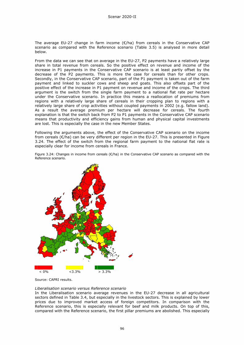
Scenar 2020-II

96

The average EU-27 change in farm income (€/ha) from cereals in the Conservative CAP scenario as compared with the Reference scenario (Table 3.5) is analysed in more detail below. From the data we can see that on average in the EU-27, P2 payments have a relatively large share in total revenue from cereals. So the positive effect on revenue and income of the increase in P1 payments in the Conservative CAP scenario is at least partly offset by the decrease of the P2 payments. This is more the case for cereals than for other crops. Secondly, in the Conservative CAP scenario, part of the P1 payment is taken out of the farm payment and linked to suckler cows and sheep and goats. This also offsets part of the positive effect of the increase in P1 payment on revenue and income of the crops. The third argument is the switch from the single farm payment to a national flat rate per hectare under the Conservative scenario. In practice this means a reallocation of premiums from regions with a relatively large share of cereals in their cropping plan to regions with a relatively large share of crop activities without coupled payments in 2002 (e.g. fallow land). As a result the average premium per hectare will decrease for cereals. The fourth explanation is that the switch back from P2 to P1 payments in the Conservative CAP scenario means that productivity and efficiency gains from human and physical capital investments are lost. This is especially the case in the new Member States. Following the arguments above, the effect of the Conservative CAP scenario on the income from cereals (€/ha) can be very different per region in the EU-27. This is presented in Figure 3.24. The effect of the switch from the regional farm payment to the national flat rate is especially clear for income from cereals in France. Figure 3.24: Changes in income from cereals (€/ha) in the Conservative CAP scenario as compared with the Reference scenario.

< 0% <3.3% > 3.3%

Source: CAPRI results. Liberalisation scenario versus Reference scenario In the Liberalisation scenario average revenues in the EU-27 decrease in all agricultural sectors defined in Table 3.4, but especially in the livestock sectors. This is explained by lower prices due to improved market access of foreign competitors. In comparison with the Reference scenario, this is especially relevant for beef and milk products. On top of this, compared with the Reference scenario, the first pillar premiums are abolished. This especially

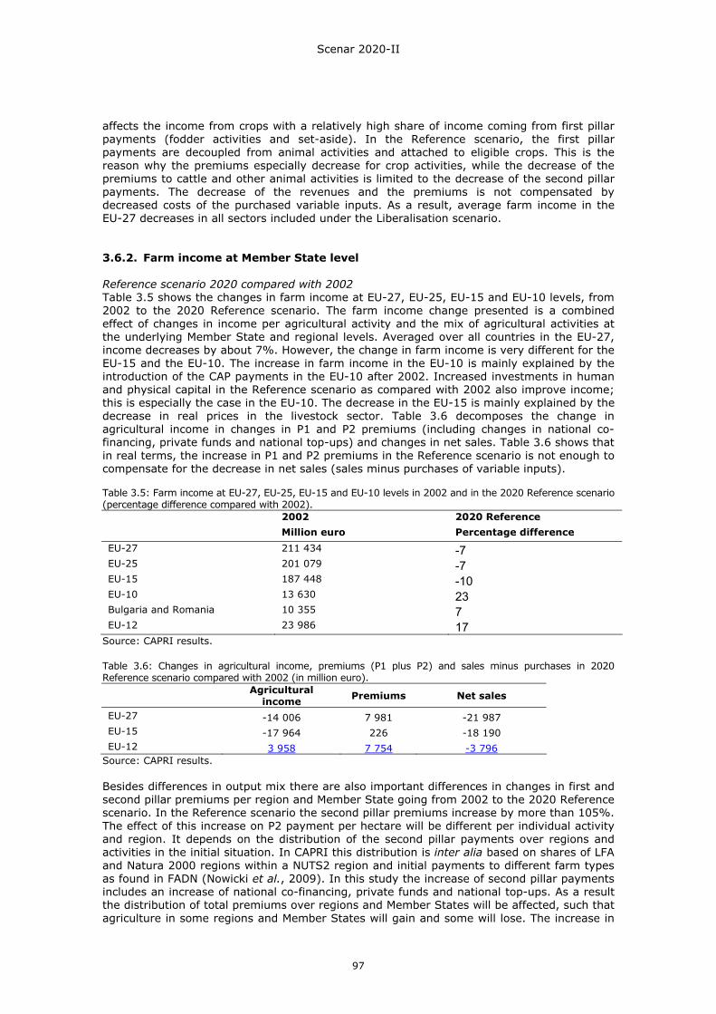
Scenar 2020-II

97

affects the income from crops with a relatively high share of income coming from first pillar payments (fodder activities and set-aside). In the Reference scenario, the first pillar payments are decoupled from animal activities and attached to eligible crops. This is the reason why the premiums especially decrease for crop activities, while the decrease of the premiums to cattle and other animal activities is limited to the decrease of the second pillar payments. The decrease of the revenues and the premiums is not compensated by decreased costs of the purchased variable inputs. As a result, average farm income in the EU-27 decreases in all sectors included under the Liberalisation scenario. 3.6.2. Farm income at Member State level Reference scenario 2020 compared with 2002 Table 3.5 shows the changes in farm income at EU-27, EU-25, EU-15 and EU-10 levels, from 2002 to the 2020 Reference scenario. The farm income change presented is a combined effect of changes in income per agricultural activity and the mix of agricultural activities at the underlying Member State and regional levels. Averaged over all countries in the EU-27, income decreases by about 7%. However, the change in farm income is very different for the EU-15 and the EU-10. The increase in farm income in the EU-10 is mainly explained by the introduction of the CAP payments in the EU-10 after 2002. Increased investments in human and physical capital in the Reference scenario as compared with 2002 also improve income; this is especially the case in the EU-10. The decrease in the EU-15 is mainly explained by the decrease in real prices in the livestock sector. Table 3.6 decomposes the change in agricultural income in changes in P1 and P2 premiums (including changes in national co-financing, private funds and national top-ups) and changes in net sales. Table 3.6 shows that in real terms, the increase in P1 and P2 premiums in the Reference scenario is not enough to compensate for the decrease in net sales (sales minus purchases of variable inputs). Table 3.5: Farm income at EU-27, EU-25, EU-15 and EU-10 levels in 2002 and in the 2020 Reference scenario (percentage difference compared with 2002). 2002 2020 Reference Million euro Percentage difference

EU-27 211 434 -7 EU-25 201 079 -7 EU-15 187 448 -10 EU-10 13 630 23 Bulgaria and Romania 10 355 7 EU-12 23 986 17

Source: CAPRI results. Table 3.6: Changes in agricultural income, premiums (P1 plus P2) and sales minus purchases in 2020 Reference scenario compared with 2002 (in million euro).

Agricultural income Premiums Net sales

EU-27 -14 006 7 981 -21 987 EU-15 -17 964 226 -18 190 EU-12 3 958 7 754 -3 796

Source: CAPRI results. Besides differences in output mix there are also important differences in changes in first and second pillar premiums per region and Member State going from 2002 to the 2020 Reference scenario. In the Reference scenario the second pillar premiums increase by more than 105%. The effect of this increase on P2 payment per hectare will be different per individual activity and region. It depends on the distribution of the second pillar payments over regions and activities in the initial situation. In CAPRI this distribution is inter alia based on shares of LFA and Natura 2000 regions within a NUTS2 region and initial payments to different farm types as found in FADN (Nowicki et al., 2009). In this study the increase of second pillar payments includes an increase of national co-financing, private funds and national top-ups. As a result the distribution of total premiums over regions and Member States will be affected, such that agriculture in some regions and Member States will gain and some will lose. The increase in

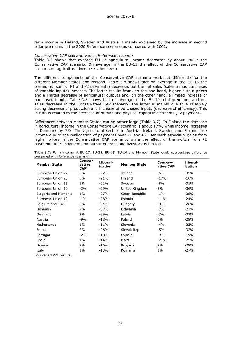
Scenar 2020-II

98

farm income in Finland, Sweden and Austria is mainly explained by the increase in second pillar premiums in the 2020 Reference scenario as compared with 2002. Conservative CAP scenario versus Reference scenario Table 3.7 shows that average EU-12 agricultural income decreases by about 1% in the Conservative CAP scenario. On average in the EU-15 the effect of the Conservative CAP scenario on agricultural income is about zero. The different components of the Conservative CAP scenario work out differently for the different Member States and regions. Table 3.8 shows that on average in the EU-15 the premiums (sum of P1 and P2 payments) decrease, but the net sales (sales minus purchases of variable inputs) increase. The latter results from, on the one hand, higher output prices and a limited decrease of agricultural outputs and, on the other hand, a limited increase of purchased inputs. Table 3.8 shows that on average in the EU-10 total premiums and net sales decrease in the Conservative CAP scenario. The latter is mainly due to a relatively strong decrease of production and increase of purchased inputs (decrease of efficiency). This in turn is related to the decrease of human and physical capital investments (P2 payment). Differences between Member States can be rather large (Table 3.7). In Finland the decrease in agricultural income in the Conservative CAP scenario is about 17%, while income increases in Denmark by 7%. The agricultural sectors in Austria, Ireland, Sweden and Finland lose income due to the reallocation of payments over P1 and P2. Denmark especially gains from higher prices in the Conservative CAP scenario, while the effect of the switch from P2 payments to P1 payments on output of crops and livestock is limited. Table 3.7: Farm income at EU-27, EU-25, EU-15, EU-10 and Member State levels (percentage difference compared with Reference scenario).

Member State Conser-vative CAP

Liberal-isation Member State Conserv-

ative CAP Liberal-isation

European Union 27 0% -22% Ireland -6% -35% European Union 25 0% -21% Finland -17% -16% European Union 15 1% -21% Sweden -8% -31% European Union 10 -2% -29% United Kingdom 2% -36% Bulgaria and Romania 1% -27% Czech Republic -1% -38% European Union 12 -1% -28% Estonia -11% -24% Belgium and Lux. 2% -34% Hungary -3% -26% Denmark 7% -37% Lithuania -7% -27% Germany 2% -29% Latvia -7% -33% Austria -9% -18% Poland 0% -28% Netherlands 1% -11% Slovenia -4% -23% France 2% -26% Slovak Rep. -5% -32% Portugal -2% -18% Cyprus -9% -19% Spain 1% -14% Malta -21% -25% Greece 2% -16% Bulgaria 2% -29% Italy 1% -13% Romania 1% -27%

Source: CAPRI results.

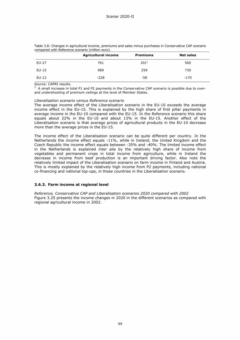
Scenar 2020-II

99

Table 3.8: Changes in agricultural income, premiums and sales minus purchases in Conservative CAP scenario compared with Reference scenario (million euro).

Agricultural income Premiums Net sales

EU-27 761 2011 560

EU-15 989 259 730

EU-12 -228 -58 -170

Source: CAPRI results. 1. A small increase in total P1 and P2 payments in the Conservative CAP scenario is possible due to over- and undershooting of premium ceilings at the level of Member States. Liberalisation scenario versus Reference scenario The average income effect of the Liberalisation scenario in the EU-10 exceeds the average income effect in the EU-15. This is explained by the high share of first pillar payments in average income in the EU-10 compared with the EU-15. In the Reference scenario this share equals about 22% in the EU-10 and about 13% in the EU-15. Another effect of the Liberalisation scenario is that average prices of agricultural products in the EU-10 decrease more than the average prices in the EU-15. The income effect of the Liberalisation scenario can be quite different per country. In the Netherlands the income effect equals -11%, while in Ireland, the United Kingdom and the Czech Republic the income effect equals between -35% and -40%. The limited income effect in the Netherlands is explained inter alia by the relatively high share of income from vegetables and permanent crops in total income from agriculture, while in Ireland the decrease in income from beef production is an important driving factor. Also note the relatively limited impact of the Liberalisation scenario on farm income in Finland and Austria. This is mostly explained by the relatively high income from P2 payments, including national co-financing and national top-ups, in these countries in the Liberalisation scenario. 3.6.3. Farm income at regional level Reference, Conservative CAP and Liberalisation scenarios 2020 compared with 2002 Figure 3.25 presents the income changes in 2020 in the different scenarios as compared with regional agricultural income in 2002.

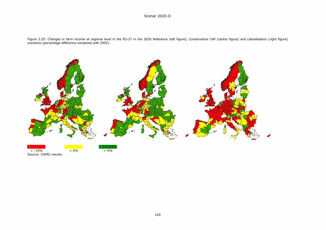
Scenar 2020-II

100

Figure 3.25: Changes in farm income at regional level in the EU-27 in the 2020 Reference (left figure), Conservative CAP (centre figure) and Liberalisation (right figure) scenarios (percentage difference compared with 2002).

< -19% < 0% > 0%

Source: CAPRI results.

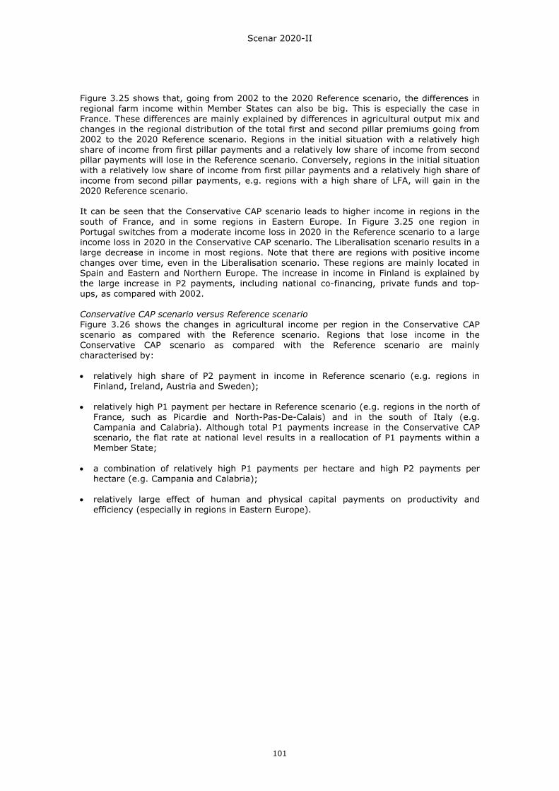
Scenar 2020-II

101

Figure 3.25 shows that, going from 2002 to the 2020 Reference scenario, the differences in regional farm income within Member States can also be big. This is especially the case in France. These differences are mainly explained by differences in agricultural output mix and changes in the regional distribution of the total first and second pillar premiums going from 2002 to the 2020 Reference scenario. Regions in the initial situation with a relatively high share of income from first pillar payments and a relatively low share of income from second pillar payments will lose in the Reference scenario. Conversely, regions in the initial situation with a relatively low share of income from first pillar payments and a relatively high share of income from second pillar payments, e.g. regions with a high share of LFA, will gain in the 2020 Reference scenario. It can be seen that the Conservative CAP scenario leads to higher income in regions in the south of France, and in some regions in Eastern Europe. In Figure 3.25 one region in Portugal switches from a moderate income loss in 2020 in the Reference scenario to a large income loss in 2020 in the Conservative CAP scenario. The Liberalisation scenario results in a large decrease in income in most regions. Note that there are regions with positive income changes over time, even in the Liberalisation scenario. These regions are mainly located in Spain and Eastern and Northern Europe. The increase in income in Finland is explained by the large increase in P2 payments, including national co-financing, private funds and top-ups, as compared with 2002. Conservative CAP scenario versus Reference scenario Figure 3.26 shows the changes in agricultural income per region in the Conservative CAP scenario as compared with the Reference scenario. Regions that lose income in the Conservative CAP scenario as compared with the Reference scenario are mainly characterised by: • relatively high share of P2 payment in income in Reference scenario (e.g. regions in

Finland, Ireland, Austria and Sweden); • relatively high P1 payment per hectare in Reference scenario (e.g. regions in the north of

France, such as Picardie and North-Pas-De-Calais) and in the south of Italy (e.g. Campania and Calabria). Although total P1 payments increase in the Conservative CAP scenario, the flat rate at national level results in a reallocation of P1 payments within a Member State;

• a combination of relatively high P1 payments per hectare and high P2 payments per

hectare (e.g. Campania and Calabria); • relatively large effect of human and physical capital payments on productivity and

efficiency (especially in regions in Eastern Europe).

Scenar 2020-II

102

Figure 3.26: Effects of the Conservative CAP scenario on farm income per region (percentage difference compared with Reference scenario).

< 0% < 2% > 2%

Source: CAPRI results. Figure 3.26 shows that within countries, the income effects can be rather different per region. In France the changes in regional agricultural income range from about -5% in Picardie to more than +7% in Limousin, Auvergne, Languedoc-Roussillon and Provence. The decrease in agricultural income in Picardie is especially explained by the decrease in first pillar payments due to a switch to a flat rate system at national level. First pillar payments increase sharply in regions with increasing agricultural income. Liberalisation scenario versus Reference scenario Figure 3.27 shows that the income effect of the Liberalisation scenario is especially large in regions in the United Kingdom, Ireland, Denmark, France, Belgium/Luxembourg, Germany and regions in Eastern Europe. Regions with a high share of income from vegetables and permanent crops are less affected by the Liberalisation scenario. Note that also in Finland and Austria agricultural income decreases compared with the 2020 Reference scenario.

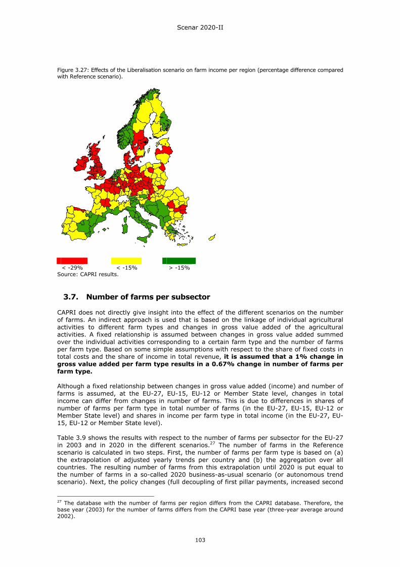
Scenar 2020-II

103

Figure 3.27: Effects of the Liberalisation scenario on farm income per region (percentage difference compared with Reference scenario).

< -29% < -15% > -15%

Source: CAPRI results.

3.7. Number of farms per subsector CAPRI does not directly give insight into the effect of the different scenarios on the number of farms. An indirect approach is used that is based on the linkage of individual agricultural activities to different farm types and changes in gross value added of the agricultural activities. A fixed relationship is assumed between changes in gross value added summed over the individual activities corresponding to a certain farm type and the number of farms per farm type. Based on some simple assumptions with respect to the share of fixed costs in total costs and the share of income in total revenue, it is assumed that a 1% change in gross value added per farm type results in a 0.67% change in number of farms per farm type. Although a fixed relationship between changes in gross value added (income) and number of farms is assumed, at the EU-27, EU-15, EU-12 or Member State level, changes in total income can differ from changes in number of farms. This is due to differences in shares of number of farms per farm type in total number of farms (in the EU-27, EU-15, EU-12 or Member State level) and shares in income per farm type in total income (in the EU-27, EU-15, EU-12 or Member State level). Table 3.9 shows the results with respect to the number of farms per subsector for the EU-27 in 2003 and in 2020 in the different scenarios.27 The number of farms in the Reference scenario is calculated in two steps. First, the number of farms per farm type is based on (a) the extrapolation of adjusted yearly trends per country and (b) the aggregation over all countries. The resulting number of farms from this extrapolation until 2020 is put equal to the number of farms in a so-called 2020 business-as-usual scenario (or autonomous trend scenario). Next, the policy changes (full decoupling of first pillar payments, increased second

27 The database with the number of farms per region differs from the CAPRI database. Therefore, the base year (2003) for the number of farms differs from the CAPRI base year (three-year average around 2002).

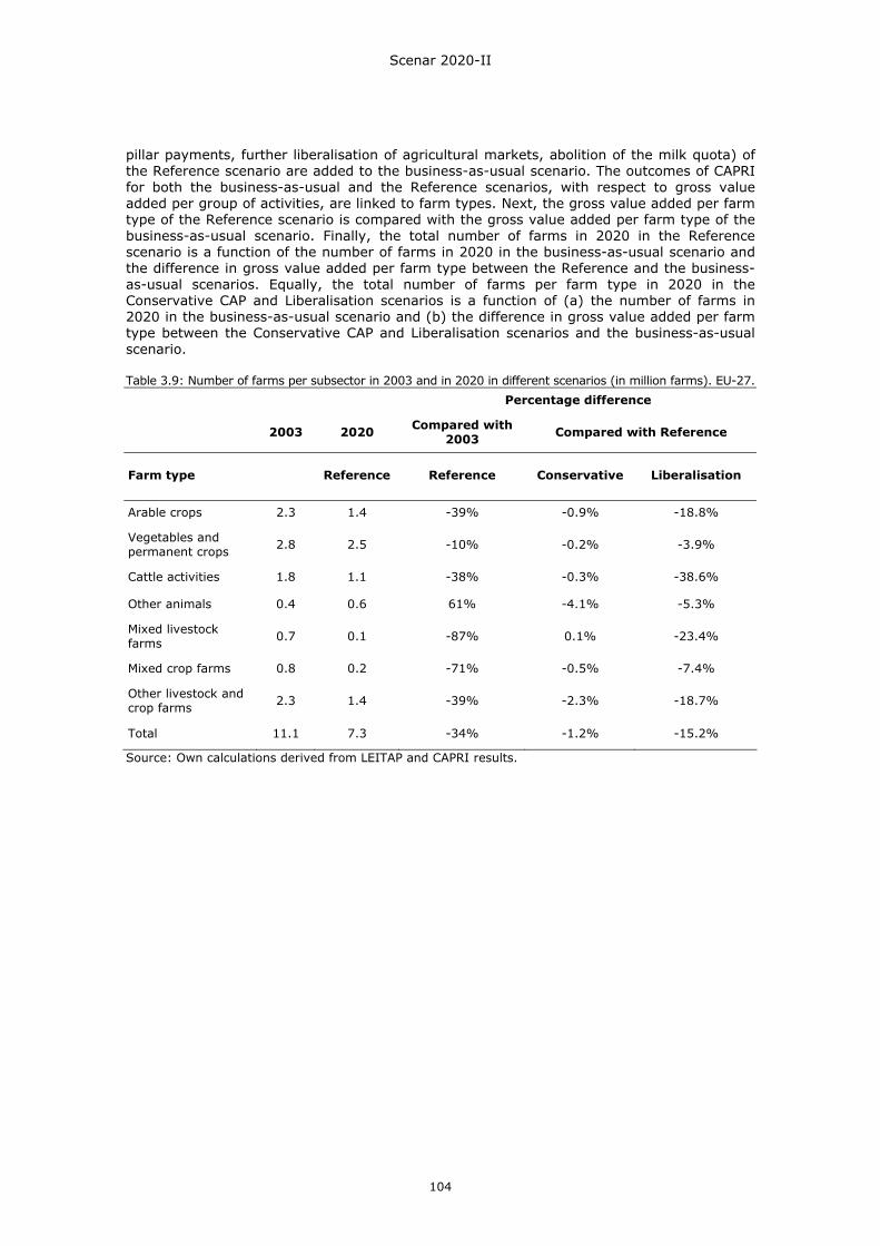
Scenar 2020-II

104

pillar payments, further liberalisation of agricultural markets, abolition of the milk quota) of the Reference scenario are added to the business-as-usual scenario. The outcomes of CAPRI for both the business-as-usual and the Reference scenarios, with respect to gross value added per group of activities, are linked to farm types. Next, the gross value added per farm type of the Reference scenario is compared with the gross value added per farm type of the business-as-usual scenario. Finally, the total number of farms in 2020 in the Reference scenario is a function of the number of farms in 2020 in the business-as-usual scenario and the difference in gross value added per farm type between the Reference and the business-as-usual scenarios. Equally, the total number of farms per farm type in 2020 in the Conservative CAP and Liberalisation scenarios is a function of (a) the number of farms in 2020 in the business-as-usual scenario and (b) the difference in gross value added per farm type between the Conservative CAP and Liberalisation scenarios and the business-as-usual scenario. Table 3.9: Number of farms per subsector in 2003 and in 2020 in different scenarios (in million farms). EU-27.

Percentage difference

2003 2020 Compared with 2003 Compared with Reference

Farm type Reference Reference Conservative Liberalisation

Arable crops 2.3 1.4 -39% -0.9% -18.8%

Vegetables and permanent crops 2.8 2.5 -10% -0.2% -3.9%

Cattle activities 1.8 1.1 -38% -0.3% -38.6%

Other animals 0.4 0.6 61% -4.1% -5.3%

Mixed livestock farms 0.7 0.1 -87% 0.1% -23.4%

Mixed crop farms 0.8 0.2 -71% -0.5% -7.4%

Other livestock and crop farms 2.3 1.4 -39% -2.3% -18.7%

Total 11.1 7.3 -34% -1.2% -15.2%

Source: Own calculations derived from LEITAP and CAPRI results.

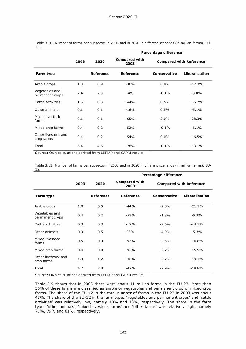
Scenar 2020-II

105

Table 3.10: Number of farms per subsector in 2003 and in 2020 in different scenarios (in million farms). EU-15. Percentage difference

2003 2020 Compared with 2003 Compared with Reference

Farm type Reference Reference Conservative Liberalisation

Arable crops 1.3 0.9 -36% 0.0% -17.3%

Vegetables and permanent crops 2.4 2.3 -4% -0.1% -3.8%

Cattle activities 1.5 0.8 -44% 0.5% -36.7%

Other animals 0.1 0.1 -16% 0.5% -5.1%

Mixed livestock farms 0.1 0.1 -65% 2.0% -28.3%

Mixed crop farms 0.4 0.2 -52% -0.1% -6.1%

Other livestock and crop farms 0.4 0.2 -54% 0.0% -16.5%

Total 6.4 4.6 -28% -0.1% -13.1%

Source: Own calculations derived from LEITAP and CAPRI results. Table 3.11: Number of farms per subsector in 2003 and in 2020 in different scenarios (in million farms). EU-12.

Percentage difference

2003 2020 Compared with 2003 Compared with Reference

Farm type Reference Reference Conservative Liberalisation

Arable crops 1.0 0.5 -44% -2.3% -21.1%

Vegetables and permanent crops 0.4 0.2 -53% -1.8% -5.9%

Cattle activities 0.3 0.3 -12% -2.6% -44.1%

Other animals 0.3 0.5 93% -4.9% -5.3%

Mixed livestock farms 0.5 0.0 -93% -2.5% -16.8%

Mixed crop farms 0.4 0.0 -92% -2.7% -15.9%

Other livestock and crop farms 1.9 1.2 -36% -2.7% -19.1%

Total 4.7 2.8 -42% -2.9% -18.8%

Source: Own calculations derived from LEITAP and CAPRI results. Table 3.9 shows that in 2003 there were about 11 million farms in the EU-27. More than 50% of these farms are classified as arable or vegetables and permanent crop or mixed crop farms. The share of the EU-12 in the total number of farms in the EU-27 in 2003 was about 43%. The share of the EU-12 in the farm types ‘vegetables and permanent crops’ and ‘cattle activities’ was relatively low, namely 13% and 18%, respectively. The share in the farm types ‘other animals’, ‘mixed livestock farms’ and ‘other farms’ was relatively high, namely 71%, 79% and 81%, respectively.

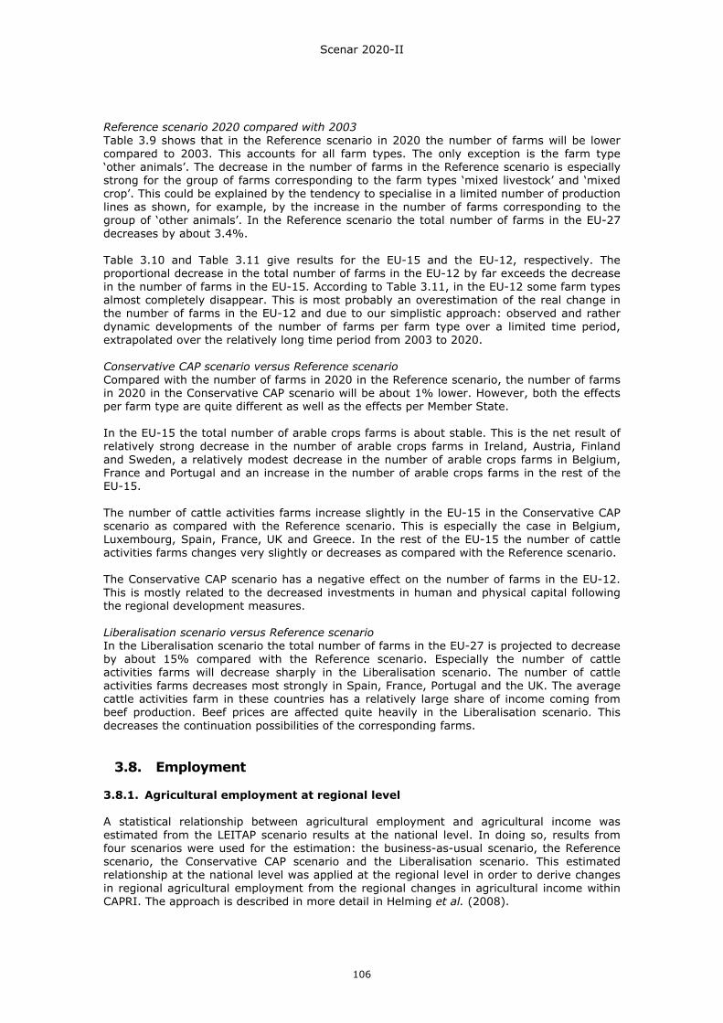
Scenar 2020-II

106

Reference scenario 2020 compared with 2003 Table 3.9 shows that in the Reference scenario in 2020 the number of farms will be lower compared to 2003. This accounts for all farm types. The only exception is the farm type ‘other animals’. The decrease in the number of farms in the Reference scenario is especially strong for the group of farms corresponding to the farm types ‘mixed livestock’ and ‘mixed crop’. This could be explained by the tendency to specialise in a limited number of production lines as shown, for example, by the increase in the number of farms corresponding to the group of ‘other animals’. In the Reference scenario the total number of farms in the EU-27 decreases by about 3.4%. Table 3.10 and Table 3.11 give results for the EU-15 and the EU-12, respectively. The proportional decrease in the total number of farms in the EU-12 by far exceeds the decrease in the number of farms in the EU-15. According to Table 3.11, in the EU-12 some farm types almost completely disappear. This is most probably an overestimation of the real change in the number of farms in the EU-12 and due to our simplistic approach: observed and rather dynamic developments of the number of farms per farm type over a limited time period, extrapolated over the relatively long time period from 2003 to 2020. Conservative CAP scenario versus Reference scenario Compared with the number of farms in 2020 in the Reference scenario, the number of farms in 2020 in the Conservative CAP scenario will be about 1% lower. However, both the effects per farm type are quite different as well as the effects per Member State. In the EU-15 the total number of arable crops farms is about stable. This is the net result of relatively strong decrease in the number of arable crops farms in Ireland, Austria, Finland and Sweden, a relatively modest decrease in the number of arable crops farms in Belgium, France and Portugal and an increase in the number of arable crops farms in the rest of the EU-15. The number of cattle activities farms increase slightly in the EU-15 in the Conservative CAP scenario as compared with the Reference scenario. This is especially the case in Belgium, Luxembourg, Spain, France, UK and Greece. In the rest of the EU-15 the number of cattle activities farms changes very slightly or decreases as compared with the Reference scenario. The Conservative CAP scenario has a negative effect on the number of farms in the EU-12. This is mostly related to the decreased investments in human and physical capital following the regional development measures. Liberalisation scenario versus Reference scenario In the Liberalisation scenario the total number of farms in the EU-27 is projected to decrease by about 15% compared with the Reference scenario. Especially the number of cattle activities farms will decrease sharply in the Liberalisation scenario. The number of cattle activities farms decreases most strongly in Spain, France, Portugal and the UK. The average cattle activities farm in these countries has a relatively large share of income coming from beef production. Beef prices are affected quite heavily in the Liberalisation scenario. This decreases the continuation possibilities of the corresponding farms.

3.8. Employment 3.8.1. Agricultural employment at regional level A statistical relationship between agricultural employment and agricultural income was estimated from the LEITAP scenario results at the national level. In doing so, results from four scenarios were used for the estimation: the business-as-usual scenario, the Reference scenario, the Conservative CAP scenario and the Liberalisation scenario. This estimated relationship at the national level was applied at the regional level in order to derive changes in regional agricultural employment from the regional changes in agricultural income within CAPRI. The approach is described in more detail in Helming et al. (2008).

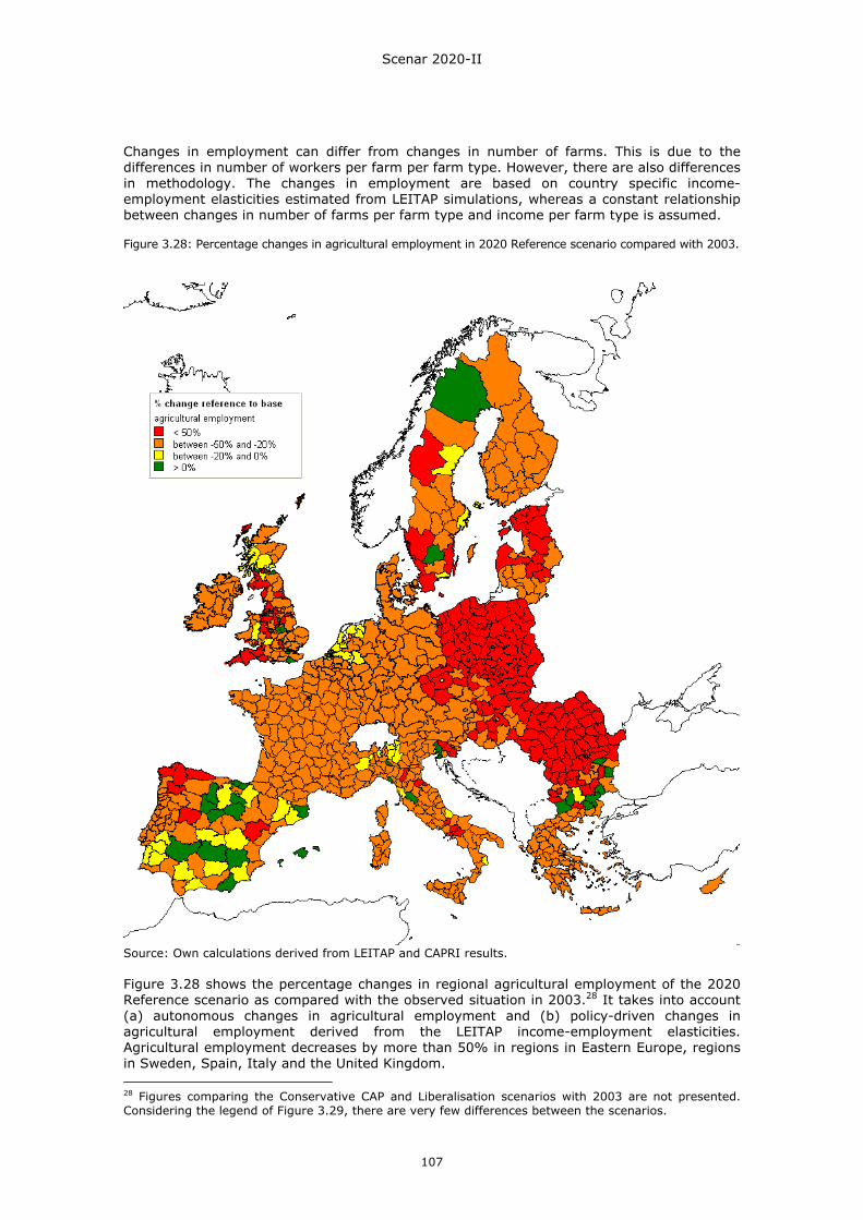
Scenar 2020-II

107

Changes in employment can differ from changes in number of farms. This is due to the differences in number of workers per farm per farm type. However, there are also differences in methodology. The changes in employment are based on country specific income-employment elasticities estimated from LEITAP simulations, whereas a constant relationship between changes in number of farms per farm type and income per farm type is assumed. Figure 3.28: Percentage changes in agricultural employment in 2020 Reference scenario compared with 2003.

Source: Own calculations derived from LEITAP and CAPRI results. Figure 3.28 shows the percentage changes in regional agricultural employment of the 2020 Reference scenario as compared with the observed situation in 2003.28 It takes into account (a) autonomous changes in agricultural employment and (b) policy-driven changes in agricultural employment derived from the LEITAP income-employment elasticities. Agricultural employment decreases by more than 50% in regions in Eastern Europe, regions in Sweden, Spain, Italy and the United Kingdom. 28 Figures comparing the Conservative CAP and Liberalisation scenarios with 2003 are not presented. Considering the legend of Figure 3.29, there are very few differences between the scenarios.

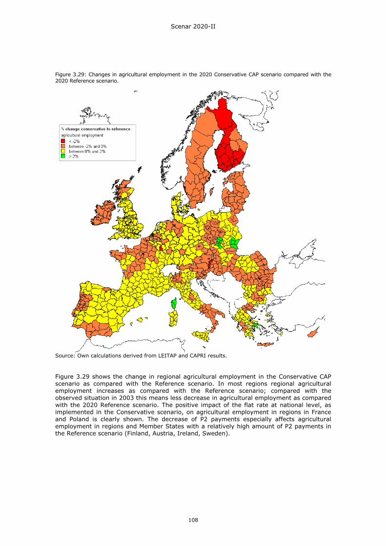
Scenar 2020-II

108

Figure 3.29: Changes in agricultural employment in the 2020 Conservative CAP scenario compared with the 2020 Reference scenario.

Source: Own calculations derived from LEITAP and CAPRI results. Figure 3.29 shows the change in regional agricultural employment in the Conservative CAP scenario as compared with the Reference scenario. In most regions regional agricultural employment increases as compared with the Reference scenario; compared with the observed situation in 2003 this means less decrease in agricultural employment as compared with the 2020 Reference scenario. The positive impact of the flat rate at national level, as implemented in the Conservative scenario, on agricultural employment in regions in France and Poland is clearly shown. The decrease of P2 payments especially affects agricultural employment in regions and Member States with a relatively high amount of P2 payments in the Reference scenario (Finland, Austria, Ireland, Sweden).

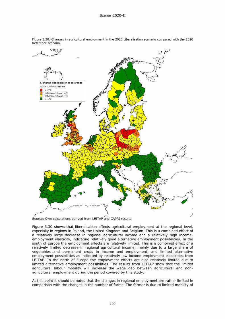
Scenar 2020-II

109

Figure 3.30: Changes in agricultural employment in the 2020 Liberalisation scenario compared with the 2020 Reference scenario.

Source: Own calculations derived from LEITAP and CAPRI results. Figure 3.30 shows that liberalisation affects agricultural employment at the regional level, especially in regions in Poland, the United Kingdom and Belgium. This is a combined effect of a relatively large decrease in regional agricultural income and a relatively high income-employment elasticity, indicating relatively good alternative employment possibilities. In the south of Europe the employment effects are relatively limited. This is a combined effect of a relatively limited decrease in regional agricultural income, mainly due to a large share of vegetables and permanent crops in income and employment, and limited alternative employment possibilities as indicated by relatively low income-employment elasticities from LEITAP. In the north of Europe the employment effects are also relatively limited due to limited alternative employment possibilities. The results from LEITAP show that the limited agricultural labour mobility will increase the wage gap between agricultural and non-agricultural employment during the period covered by this study. At this point it should be noted that the changes in regional employment are rather limited in comparison with the changes in the number of farms. The former is due to limited mobility of

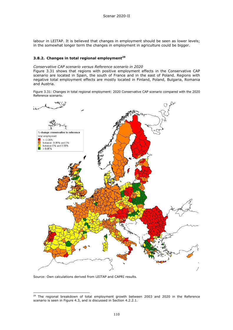
Scenar 2020-II

110

labour in LEITAP. It is believed that changes in employment should be seen as lower levels; in the somewhat longer term the changes in employment in agriculture could be bigger. 3.8.2. Changes in total regional employment29 Conservative CAP scenario versus Reference scenario in 2020 Figure 3.31 shows that regions with positive employment effects in the Conservative CAP scenario are located in Spain, the south of France and in the east of Poland. Regions with negative total employment effects are mostly located in Finland, Poland, Bulgaria, Romania and Austria. Figure 3.31: Changes in total regional employment: 2020 Conservative CAP scenario compared with the 2020 Reference scenario.

Source: Own calculations derived from LEITAP and CAPRI results.

29 The regional breakdown of total employment growth between 2003 and 2020 in the Reference scenario is seen in Figure 4.3, and is discussed in Section 4.2.2.1.

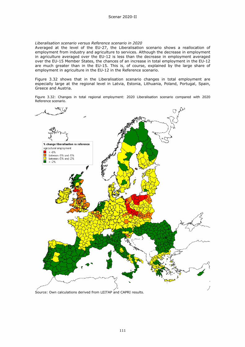
Scenar 2020-II

111

Liberalisation scenario versus Reference scenario in 2020 Averaged at the level of the EU-27, the Liberalisation scenario shows a reallocation of employment from industry and agriculture to services. Although the decrease in employment in agriculture averaged over the EU-12 is less than the decrease in employment averaged over the EU-15 Member States, the chances of an increase in total employment in the EU-12 are much greater than in the EU-15. This is, of course, explained by the large share of employment in agriculture in the EU-12 in the Reference scenario. Figure 3.32 shows that in the Liberalisation scenario changes in total employment are especially large at the regional level in Latvia, Estonia, Lithuania, Poland, Portugal, Spain, Greece and Austria. Figure 3.32: Changes in total regional employment: 2020 Liberalisation scenario compared with 2020 Reference scenario.

Source: Own calculations derived from LEITAP and CAPRI results.

Scenar 2020-II

112

3.9. Sensitivity analysis 3.9.1. Sensitivity analysis for the Reference scenario The sensitivity analysis (SA) illustrates the impact of key assumptions made for the Reference scenario. The following SA scenarios have been calculated for the Reference scenario: • Different assumptions on the composition of biomass for the production of

biofuels (2GBiofuel)30 o Under the Reference scenario we assume that 1st generation biofuels will contribute

7 percentage points of the mandatory blending rate of 10%cent in 2020 (see Table 1.2). 3% is assumed to be contributed by 2nd generation biomass production, which is assumed to be grown on land which is no longer available for agricultural production.

o Under the SA it is assumed that 1st generation biofuels contribute only 5 percentage points to the Renewable Energy Directive target and another 2 percentage points stem from 2nd generation biomass. The total contribution of 2nd generation biomass production is now 5%.

o It is also assumed that the production of 2nd generation biomass is not done by farmers but by other non-agricultural sectors (e.g. forestry). Therefore, 2nd generation biomass production does not contribute to primary agricultural production and income.

• High and low crude oil prices

o It is assumed that crude oil prices are 50% higher and also 50% lower compared with the crude oil price under the Reference scenario with a crude oil price of 70 USD/bbl.

• High and low agricultural world prices

o It is assumed that world prices for agricultural products are on average 10% higher and 20% lower compared with the agricultural world prices under the Reference scenario.

o This has been implemented by a systematic variation of productivity growth rates for different agricultural commodities in non-EU countries and regions.

The discussion of the outcome of the SA focuses on the following items: production, income from agriculture, land prices and land use. The results will be discussed in a thematic way in graphs which are described separately: • Change in aggregate crop and biofuel crop production, 2007–2020, in per cent for EU-27. • Change in agricultural income, EU-27, 2007–2020, in per cent for primary agriculture,

arable production and livestock production. • Change in land prices and use, 2007–2020, in per cent for EU-27.

30 The current version of LEITAP does not model 2nd generation biofuels explicitly. This is due to the uncertain nature of cost, technology and market structures of 2nd generation biofuels. To address this shortcoming we assume that 2nd generation biofuels are produced outside agriculture and on non-agricultural land. As part of the 2nd generation biofuels is expected to be produced within the agricultural sector, the negative impact of a shift from 1st to 2nd generation biofuels on production, land and income can be interpreted as on the high end.

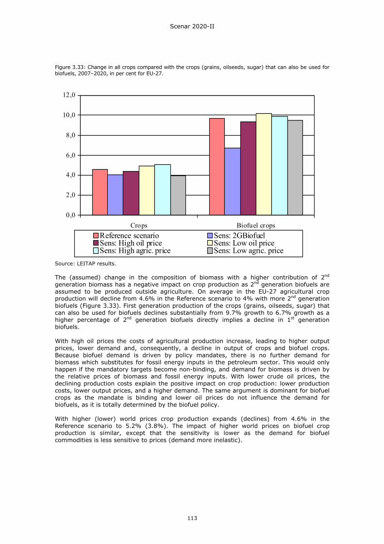
Scenar 2020-II

113

0,0

2,0

4,0

6,0

8,0

10,0

12,0

Crops Biofuel cropsReference scenario Sens: 2GBiofuelSens: High oil price Sens: Low oil priceSens: High agric. price Sens: Low agric. price

Figure 3.33: Change in all crops compared with the crops (grains, oilseeds, sugar) that can also be used for biofuels, 2007–2020, in per cent for EU-27.

Source: LEITAP results. The (assumed) change in the composition of biomass with a higher contribution of 2nd generation biomass has a negative impact on crop production as 2nd generation biofuels are assumed to be produced outside agriculture. On average in the EU-27 agricultural crop production will decline from 4.6% in the Reference scenario to 4% with more 2nd generation biofuels (Figure 3.33). First generation production of the crops (grains, oilseeds, sugar) that can also be used for biofuels declines substantially from 9.7% growth to 6.7% growth as a higher percentage of 2nd generation biofuels directly implies a decline in 1st generation biofuels. With high oil prices the costs of agricultural production increase, leading to higher output prices, lower demand and, consequently, a decline in output of crops and biofuel crops. Because biofuel demand is driven by policy mandates, there is no further demand for biomass which substitutes for fossil energy inputs in the petroleum sector. This would only happen if the mandatory targets become non-binding, and demand for biomass is driven by the relative prices of biomass and fossil energy inputs. With lower crude oil prices, the declining production costs explain the positive impact on crop production: lower production costs, lower output prices, and a higher demand. The same argument is dominant for biofuel crops as the mandate is binding and lower oil prices do not influence the demand for biofuels, as it is totally determined by the biofuel policy. With higher (lower) world prices crop production expands (declines) from 4.6% in the Reference scenario to 5.2% (3.8%). The impact of higher world prices on biofuel crop production is similar, except that the sensitivity is lower as the demand for biofuel commodities is less sensitive to prices (demand more inelastic).

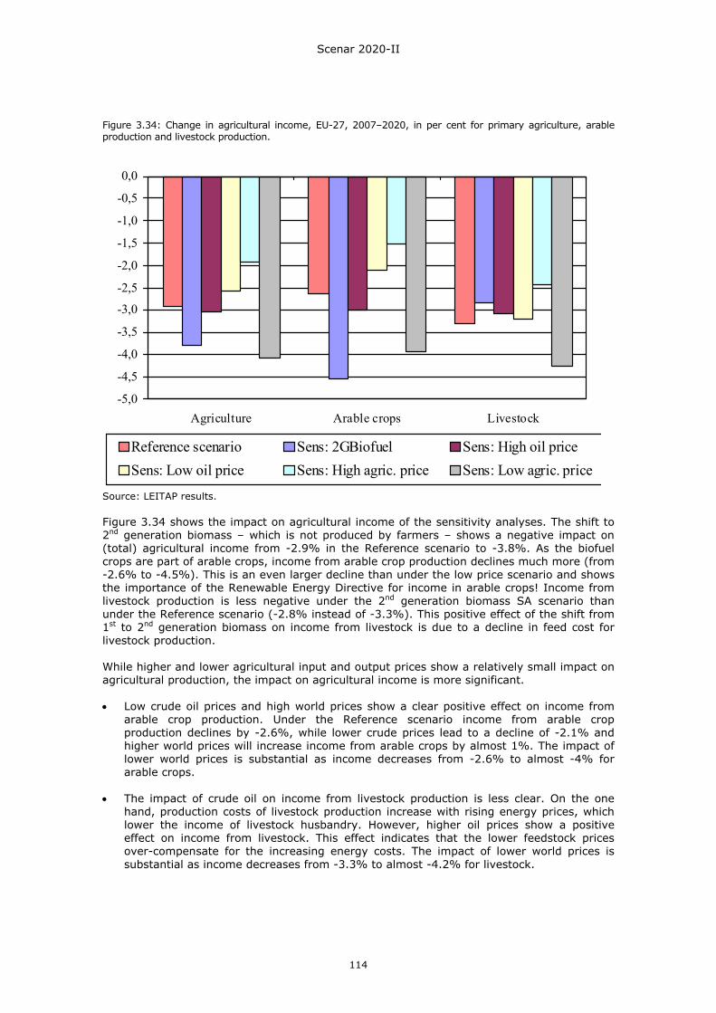
Scenar 2020-II

114

-5,0

-4,5

-4,0

-3,5

-3,0

-2,5

-2,0

-1,5

-1,0

-0,5

0,0

Agriculture Arable crops Livestock

Reference scenario Sens: 2GBiofuel Sens: High oil priceSens: Low oil price Sens: High agric. price Sens: Low agric. price

Figure 3.34: Change in agricultural income, EU-27, 2007–2020, in per cent for primary agriculture, arable production and livestock production.

Source: LEITAP results. Figure 3.34 shows the impact on agricultural income of the sensitivity analyses. The shift to 2nd generation biomass – which is not produced by farmers – shows a negative impact on (total) agricultural income from -2.9% in the Reference scenario to -3.8%. As the biofuel crops are part of arable crops, income from arable crop production declines much more (from -2.6% to -4.5%). This is an even larger decline than under the low price scenario and shows the importance of the Renewable Energy Directive for income in arable crops! Income from livestock production is less negative under the 2nd generation biomass SA scenario than under the Reference scenario (-2.8% instead of -3.3%). This positive effect of the shift from 1st to 2nd generation biomass on income from livestock is due to a decline in feed cost for livestock production. While higher and lower agricultural input and output prices show a relatively small impact on agricultural production, the impact on agricultural income is more significant. • Low crude oil prices and high world prices show a clear positive effect on income from

arable crop production. Under the Reference scenario income from arable crop production declines by -2.6%, while lower crude prices lead to a decline of -2.1% and higher world prices will increase income from arable crops by almost 1%. The impact of lower world prices is substantial as income decreases from -2.6% to almost -4% for arable crops.

• The impact of crude oil on income from livestock production is less clear. On the one

hand, production costs of livestock production increase with rising energy prices, which lower the income of livestock husbandry. However, higher oil prices show a positive effect on income from livestock. This effect indicates that the lower feedstock prices over-compensate for the increasing energy costs. The impact of lower world prices is substantial as income decreases from -3.3% to almost -4.2% for livestock.

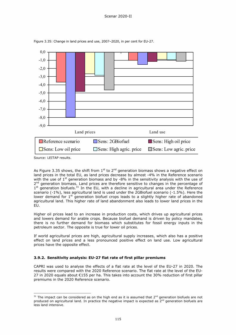
Scenar 2020-II

115

-9,0

-8,0

-7,0

-6,0

-5,0

-4,0

-3,0

-2,0

-1,0

0,0

Land prices Land use

Reference scenario Sens: 2GBiofuel Sens: High oil priceSens: Low oil price Sens: High agric. price Sens: Low agric. price

Figure 3.35: Change in land prices and use, 2007–2020, in per cent for EU-27.

Source: LEITAP results. As Figure 3.35 shows, the shift from 1st to 2nd generation biomass shows a negative effect on land prices in the total EU, as land prices decrease by almost -4% in the Reference scenario with the use of 1st generation biomass and by -8% in the sensitivity analysis with the use of 2nd generation biomass. Land prices are therefore sensitive to changes in the percentage of 1st generation biofuels.31 In the EU, with a decline in agricultural area under the Reference scenario (-1%), less agricultural land is used under the 2GBiofuel scenario (-1.5%). Here the lower demand for 1st generation biofuel crops leads to a slightly higher rate of abandoned agricultural land. This higher rate of land abandonment also leads to lower land prices in the EU. Higher oil prices lead to an increase in production costs, which drives up agricultural prices and lowers demand for arable crops. Because biofuel demand is driven by policy mandates, there is no further demand for biomass which substitutes for fossil energy inputs in the petroleum sector. The opposite is true for lower oil prices. If world agricultural prices are high, agricultural supply increases, which also has a positive effect on land prices and a less pronounced positive effect on land use. Low agricultural prices have the opposite effect. 3.9.2. Sensitivity analysis: EU-27 flat rate of first pillar premiums CAPRI was used to analyse the effects of a flat rate at the level of the EU-27 in 2020. The results were compared with the 2020 Reference scenario. The flat rate at the level of the EU-27 in 2020 equals about €155 per ha. This takes into account the 30% reduction of first pillar premiums in the 2020 Reference scenario.

31 The impact can be considered as on the high end as it is assumed that 2nd generation biofuels are not produced on agricultural land. In practice the negative impact is expected as 2nd generation biofuels are less land intensive.

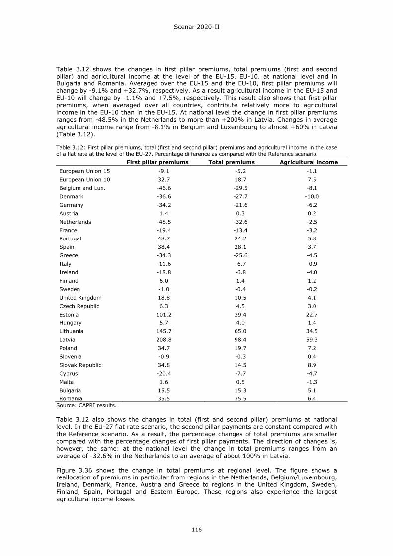
Scenar 2020-II

116

Table 3.12 shows the changes in first pillar premiums, total premiums (first and second pillar) and agricultural income at the level of the EU-15, EU-10, at national level and in Bulgaria and Romania. Averaged over the EU-15 and the EU-10, first pillar premiums will change by -9.1% and +32.7%, respectively. As a result agricultural income in the EU-15 and EU-10 will change by -1.1% and +7.5%, respectively. This result also shows that first pillar premiums, when averaged over all countries, contribute relatively more to agricultural income in the EU-10 than in the EU-15. At national level the change in first pillar premiums ranges from -48.5% in the Netherlands to more than +200% in Latvia. Changes in average agricultural income range from -8.1% in Belgium and Luxembourg to almost +60% in Latvia (Table 3.12). Table 3.12: First pillar premiums, total (first and second pillar) premiums and agricultural income in the case of a flat rate at the level of the EU-27. Percentage difference as compared with the Reference scenario.

First pillar premiums Total premiums Agricultural income

European Union 15 -9.1 -5.2 -1.1 European Union 10 32.7 18.7 7.5 Belgium and Lux. -46.6 -29.5 -8.1 Denmark -36.6 -27.7 -10.0 Germany -34.2 -21.6 -6.2 Austria 1.4 0.3 0.2 Netherlands -48.5 -32.6 -2.5 France -19.4 -13.4 -3.2 Portugal 48.7 24.2 5.8 Spain 38.4 28.1 3.7 Greece -34.3 -25.6 -4.5 Italy -11.6 -6.7 -0.9 Ireland -18.8 -6.8 -4.0 Finland 6.0 1.4 1.2 Sweden -1.0 -0.4 -0.2 United Kingdom 18.8 10.5 4.1 Czech Republic 6.3 4.5 3.0 Estonia 101.2 39.4 22.7 Hungary 5.7 4.0 1.4 Lithuania 145.7 65.0 34.5 Latvia 208.8 98.4 59.3 Poland 34.7 19.7 7.2 Slovenia -0.9 -0.3 0.4 Slovak Republic 34.8 14.5 8.9 Cyprus -20.4 -7.7 -4.7 Malta 1.6 0.5 -1.3 Bulgaria 15.5 15.3 5.1 Romania 35.5 35.5 6.4

Source: CAPRI results. Table 3.12 also shows the changes in total (first and second pillar) premiums at national level. In the EU-27 flat rate scenario, the second pillar payments are constant compared with the Reference scenario. As a result, the percentage changes of total premiums are smaller compared with the percentage changes of first pillar payments. The direction of changes is, however, the same: at the national level the change in total premiums ranges from an average of -32.6% in the Netherlands to an average of about 100% in Latvia. Figure 3.36 shows the change in total premiums at regional level. The figure shows a reallocation of premiums in particular from regions in the Netherlands, Belgium/Luxembourg, Ireland, Denmark, France, Austria and Greece to regions in the United Kingdom, Sweden, Finland, Spain, Portugal and Eastern Europe. These regions also experience the largest agricultural income losses.

Scenar 2020-II

117

Figure 3.36: Change in total (first and second pillar) premiums at the regional level in the case of a flat rate at the level of the EU-27. Percentage difference as compared with the Reference scenario.

< -0% > 0% Source: CAPRI results. Effects at sector and national and regional level (example for cereals) At national level, income from cereals production decreases by about 30% in Belgium/Luxembourg and Denmark, by about 15% in Germany and about 10% in France, Greece and Ireland. Income from cereals increases by about more than 30% in Estonia, Lithuania and Latvia and by about 10% in the United Kingdom, Spain and Poland. Regional effects can be quite different from the national average.

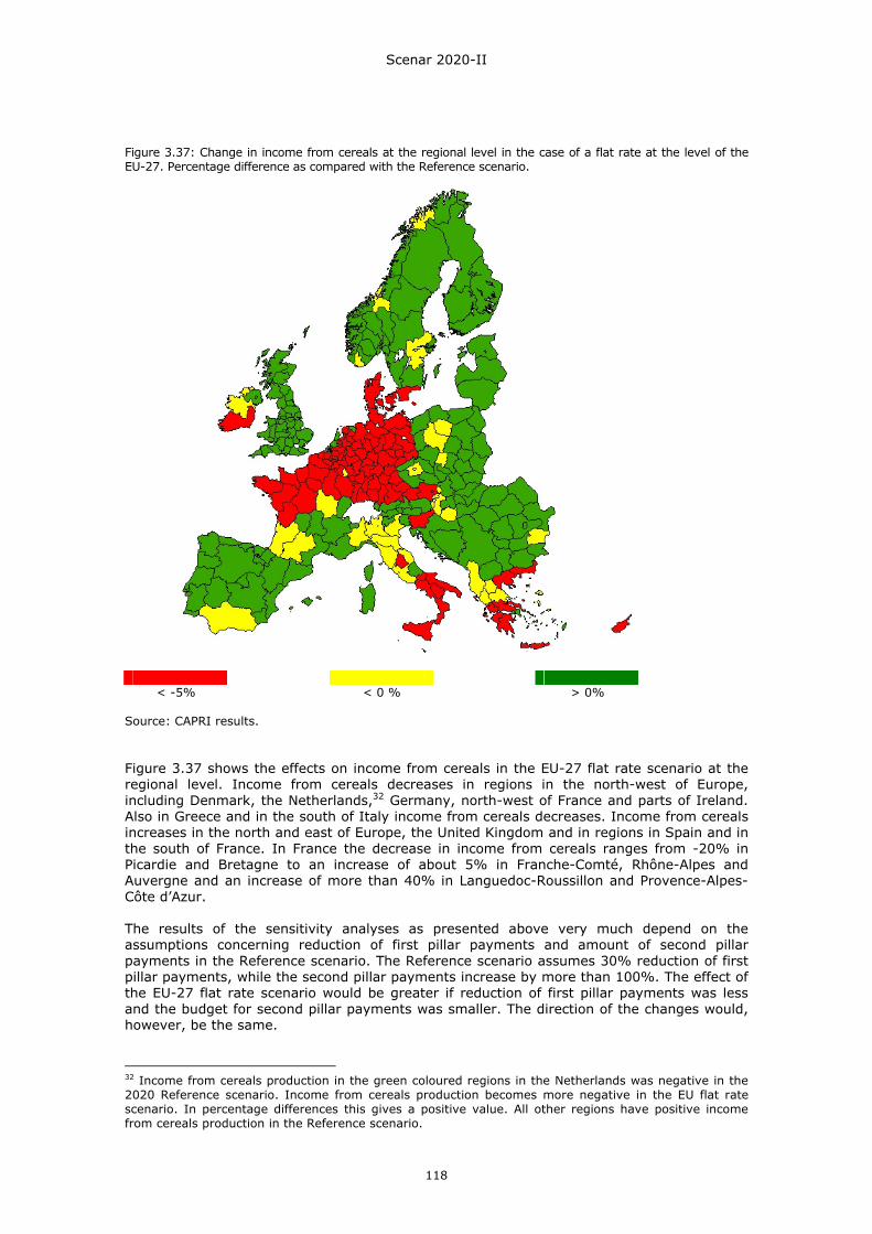
Scenar 2020-II

118

Figure 3.37: Change in income from cereals at the regional level in the case of a flat rate at the level of the EU-27. Percentage difference as compared with the Reference scenario.

< -5% < 0 % > 0% Source: CAPRI results. Figure 3.37 shows the effects on income from cereals in the EU-27 flat rate scenario at the regional level. Income from cereals decreases in regions in the north-west of Europe, including Denmark, the Netherlands,32 Germany, north-west of France and parts of Ireland. Also in Greece and in the south of Italy income from cereals decreases. Income from cereals increases in the north and east of Europe, the United Kingdom and in regions in Spain and in the south of France. In France the decrease in income from cereals ranges from -20% in Picardie and Bretagne to an increase of about 5% in Franche-Comté, Rhône-Alpes and Auvergne and an increase of more than 40% in Languedoc-Roussillon and Provence-Alpes-Côte d’Azur. The results of the sensitivity analyses as presented above very much depend on the assumptions concerning reduction of first pillar payments and amount of second pillar payments in the Reference scenario. The Reference scenario assumes 30% reduction of first pillar payments, while the second pillar payments increase by more than 100%. The effect of the EU-27 flat rate scenario would be greater if reduction of first pillar payments was less and the budget for second pillar payments was smaller. The direction of the changes would, however, be the same.

32 Income from cereals production in the green coloured regions in the Netherlands was negative in the 2020 Reference scenario. Income from cereals production becomes more negative in the EU flat rate scenario. In percentage differences this gives a positive value. All other regions have positive income from cereals production in the Reference scenario.

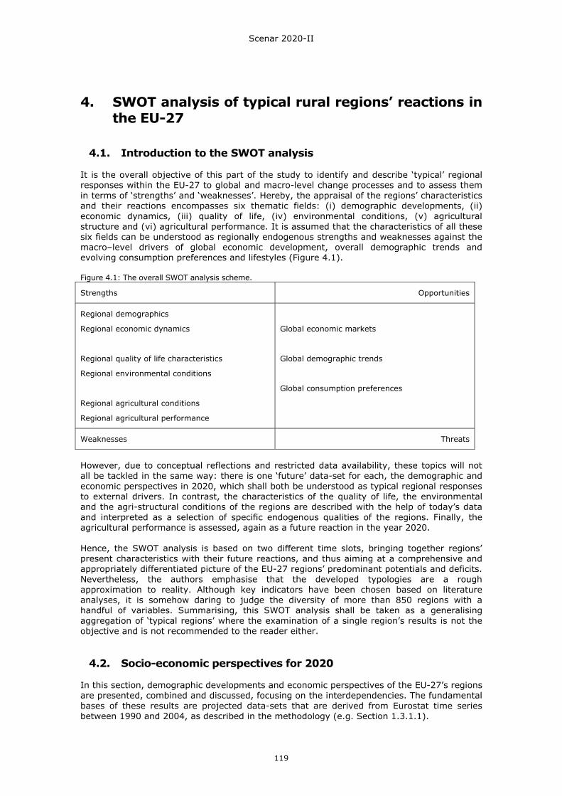
Scenar 2020-II

119

4. SWOT analysis of typical rural regions’ reactions in the EU-27

4.1. Introduction to the SWOT analysis It is the overall objective of this part of the study to identify and describe ‘typical’ regional responses within the EU-27 to global and macro-level change processes and to assess them in terms of ‘strengths’ and ‘weaknesses’. Hereby, the appraisal of the regions’ characteristics and their reactions encompasses six thematic fields: (i) demographic developments, (ii) economic dynamics, (iii) quality of life, (iv) environmental conditions, (v) agricultural structure and (vi) agricultural performance. It is assumed that the characteristics of all these six fields can be understood as regionally endogenous strengths and weaknesses against the macro–level drivers of global economic development, overall demographic trends and evolving consumption preferences and lifestyles (Figure 4.1). Figure 4.1: The overall SWOT analysis scheme.

Strengths Opportunities

Regional demographics

Regional economic dynamics

Regional quality of life characteristics

Regional environmental conditions

Regional agricultural conditions

Regional agricultural performance

Global economic markets

Global demographic trends

Global consumption preferences

Weaknesses Threats

However, due to conceptual reflections and restricted data availability, these topics will not all be tackled in the same way: there is one ‘future’ data-set for each, the demographic and economic perspectives in 2020, which shall both be understood as typical regional responses to external drivers. In contrast, the characteristics of the quality of life, the environmental and the agri-structural conditions of the regions are described with the help of today’s data and interpreted as a selection of specific endogenous qualities of the regions. Finally, the agricultural performance is assessed, again as a future reaction in the year 2020. Hence, the SWOT analysis is based on two different time slots, bringing together regions’ present characteristics with their future reactions, and thus aiming at a comprehensive and appropriately differentiated picture of the EU-27 regions’ predominant potentials and deficits. Nevertheless, the authors emphasise that the developed typologies are a rough approximation to reality. Although key indicators have been chosen based on literature analyses, it is somehow daring to judge the diversity of more than 850 regions with a handful of variables. Summarising, this SWOT analysis shall be taken as a generalising aggregation of ‘typical regions’ where the examination of a single region’s results is not the objective and is not recommended to the reader either.

4.2. Socio-economic perspectives for 2020 In this section, demographic developments and economic perspectives of the EU-27’s regions are presented, combined and discussed, focusing on the interdependencies. The fundamental bases of these results are projected data-sets that are derived from Eurostat time series between 1990 and 2004, as described in the methodology (e.g. Section 1.3.1.1).

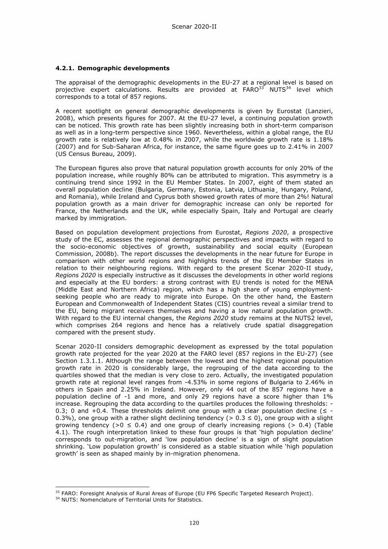
Scenar 2020-II

120

4.2.1. Demographic developments The appraisal of the demographic developments in the EU-27 at a regional level is based on projective expert calculations. Results are provided at FARO33 NUTS34 level which corresponds to a total of 857 regions. A recent spotlight on general demographic developments is given by Eurostat (Lanzieri, 2008), which presents figures for 2007. At the EU-27 level, a continuing population growth can be noticed. This growth rate has been slightly increasing both in short-term comparison as well as in a long-term perspective since 1960. Nevertheless, within a global range, the EU growth rate is relatively low at 0.48% in 2007, while the worldwide growth rate is 1.18% (2007) and for Sub-Saharan Africa, for instance, the same figure goes up to 2.41% in 2007 (US Census Bureau, 2009). The European figures also prove that natural population growth accounts for only 20% of the population increase, while roughly 80% can be attributed to migration. This asymmetry is a continuing trend since 1992 in the EU Member States. In 2007, eight of them stated an overall population decline (Bulgaria, Germany, Estonia, Latvia, Lithuania¸ Hungary, Poland, and Romania), while Ireland and Cyprus both showed growth rates of more than 2%! Natural population growth as a main driver for demographic increase can only be reported for France, the Netherlands and the UK, while especially Spain, Italy and Portugal are clearly marked by immigration. Based on population development projections from Eurostat, Regions 2020, a prospective study of the EC, assesses the regional demographic perspectives and impacts with regard to the socio-economic objectives of growth, sustainability and social equity (European Commission, 2008b). The report discusses the developments in the near future for Europe in comparison with other world regions and highlights trends of the EU Member States in relation to their neighbouring regions. With regard to the present Scenar 2020-II study, Regions 2020 is especially instructive as it discusses the developments in other world regions and especially at the EU borders: a strong contrast with EU trends is noted for the MENA (Middle East and Northern Africa) region, which has a high share of young employment-seeking people who are ready to migrate into Europe. On the other hand, the Eastern European and Commonwealth of Independent States (CIS) countries reveal a similar trend to the EU, being migrant receivers themselves and having a low natural population growth. With regard to the EU internal changes, the Regions 2020 study remains at the NUTS2 level, which comprises 264 regions and hence has a relatively crude spatial disaggregation compared with the present study. Scenar 2020-II considers demographic development as expressed by the total population growth rate projected for the year 2020 at the FARO level (857 regions in the EU-27) (see Section 1.3.1.1. Although the range between the lowest and the highest regional population growth rate in 2020 is considerably large, the regrouping of the data according to the quartiles showed that the median is very close to zero. Actually, the investigated population growth rate at regional level ranges from -4.53% in some regions of Bulgaria to 2.46% in others in Spain and 2.25% in Ireland. However, only 44 out of the 857 regions have a population decline of -1 and more, and only 29 regions have a score higher than 1% increase. Regrouping the data according to the quartiles produces the following thresholds: -0.3; 0 and +0.4. These thresholds delimit one group with a clear population decline (≤ -0.3%), one group with a rather slight declining tendency (> 0.3 ≤ 0), one group with a slight growing tendency (>0 ≤ 0.4) and one group of clearly increasing regions (> 0.4) (Table 4.1). The rough interpretation linked to these four groups is that ‘high population decline’ corresponds to out-migration, and ‘low population decline’ is a sign of slight population shrinking. ‘Low population growth’ is considered as a stable situation while ‘high population growth’ is seen as shaped mainly by in-migration phenomena.

33 FARO: Foresight Analysis of Rural Areas of Europe (EU FP6 Specific Targeted Research Project). 34 NUTS: Nomenclature of Territorial Units for Statistics.

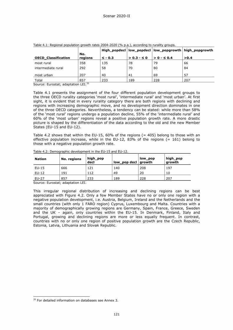
Scenar 2020-II

121

Table 4.1: Regional population growth rates 2004-2020 (% p.a.), according to rurality groups.

High_popdecl low_popdecl low_popgrowth high_popgrowth

OECD_Classification No. regions ≤ - 0.3 > 0.3 - ≤ 0 > 0 - ≤ 0.4 >0.4

most rural 358 135 78 79 66 intermediate rural 292 58 70 80 84

most urban 207 40 41 69 57

Total 857 233 189 228 207 Source: Eurostat; adaptation LEI.35 Table 4.1 presents the assignment of the four different population development groups to the three OECD rurality categories ‘most rural’, ‘intermediate rural’ and ‘most urban’. At first sight, it is evident that in every rurality category there are both regions with declining and regions with increasing demographic move, and no development direction dominates in one of the three OECD categories. Nevertheless, a tendency can be stated: while more than 58% of the ‘most rural’ regions undergo a population decline, 55% of the ‘intermediate rural’ and 60% of the ‘most urban’ regions reveal a positive population growth rate. A more drastic picture is shaped by the differentiation of the data according to the old and the new Member States (EU-15 and EU-12). Table 4.2 shows that within the EU-15, 60% of the regions (= 405) belong to those with an effective population increase, while in the EU-12, 83% of the regions (= 161) belong to those with a negative population growth rate. Table 4.2: Demographic development in the EU-15 and EU-12.

Nation No. regions high_pop decl low_pop decl

low_pop growth

high_pop growth

EU-15 666 121 140 208 197 EU-12 191 112 49 20 10

EU-27 857 233 189 228 207 Source: Eurostat; adaptation LEI. This irregular regional distribution of increasing and declining regions can be best appreciated with Figure 4.2. Only a few Member States have no or only one region with a negative population development, i.e. Austria, Belgium, Ireland and the Netherlands and the small countries (with only 1 FARO region) Cyprus, Luxembourg and Malta. Countries with a majority of demographically growing regions are Germany, Spain, France, Greece, Sweden and the UK – again, only countries within the EU-15. In Denmark, Finland, Italy and Portugal, growing and declining regions are more or less equally frequent. In contrast, countries with no or only one region of positive population growth are the Czech Republic, Estonia, Latvia, Lithuania and Slovak Republic.

35 For detailed information on databases see Annex 3.

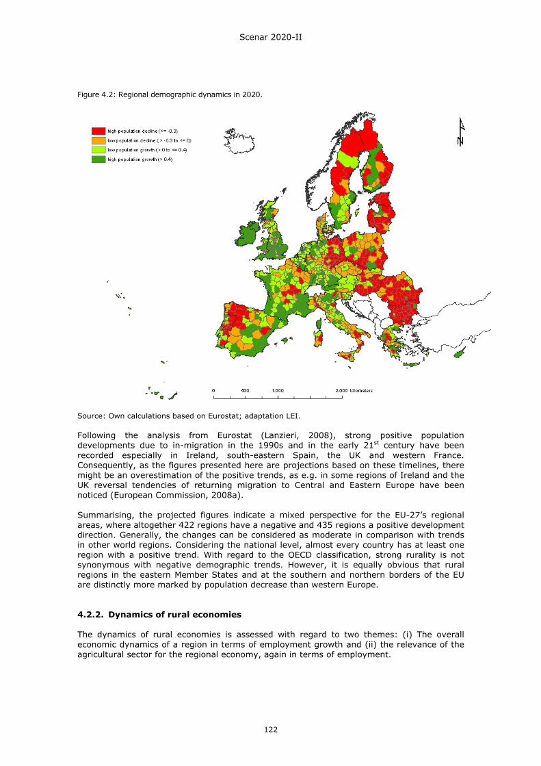
Scenar 2020-II

122

Figure 4.2: Regional demographic dynamics in 2020.

Source: Own calculations based on Eurostat; adaptation LEI. Following the analysis from Eurostat (Lanzieri, 2008), strong positive population developments due to in-migration in the 1990s and in the early 21st century have been recorded especially in Ireland, south-eastern Spain, the UK and western France. Consequently, as the figures presented here are projections based on these timelines, there might be an overestimation of the positive trends, as e.g. in some regions of Ireland and the UK reversal tendencies of returning migration to Central and Eastern Europe have been noticed (European Commission, 2008a). Summarising, the projected figures indicate a mixed perspective for the EU-27’s regional areas, where altogether 422 regions have a negative and 435 regions a positive development direction. Generally, the changes can be considered as moderate in comparison with trends in other world regions. Considering the national level, almost every country has at least one region with a positive trend. With regard to the OECD classification, strong rurality is not synonymous with negative demographic trends. However, it is equally obvious that rural regions in the eastern Member States and at the southern and northern borders of the EU are distinctly more marked by population decrease than western Europe. 4.2.2. Dynamics of rural economies The dynamics of rural economies is assessed with regard to two themes: (i) The overall economic dynamics of a region in terms of employment growth and (ii) the relevance of the agricultural sector for the regional economy, again in terms of employment.

Scenar 2020-II

123

4.2.2.1. Regional employment growth

Appreciating the potentials and limits of rural regions’ economic development is of crucial interest for the design and implementation of responsive policies. Selected studies at the European level have extensively explored and consolidated a range of indicators such as labour productivity, employment growth and workforce education (European Commission, 2008b; Terluin, 2003). In the original Scenar 2020 study, the guiding indicator for dynamics of rural economies was the employment growth rate, which was contrasted with the share of agricultural employment (Nowicki et al., 2007). In the following, the employment growth rate data are presented which have been updated since then and complemented with the data for Bulgaria and Romania (see Section 1.3.1.2). Based on a projected employment growth rate for the year 2020, three groups of differing economic performances were built in a deliberated manner (Figure 4.3). A distinctly positive perspective was set for those regions that stand out with an employment growth rate of more than 0.5% per year. On the other hand, a negative trend was attributed to those regions where the employment growth rate is below 0. Obviously, most European regions fall in between these two ranges. On this basis, the 857 FARO regions were split into 142 regions with a negative economic development perspective, where the employment rate is declining (‘gamma’), 561 regions with a moderate economic perspective (‘beta’) and 154 regions with a clear positive economic perspective (‘alpha’). As the map indicates, in nearly all Member States we find regions from all three types. Exceptions are Bulgaria and Romania, for which a uniform growth rate has been assumed due to considerable data uncertainties. Another exceptional situation can obviously be found in Spain and Ireland, where the economically performing regions largely dominate. This, of course, is a consequence of the very optimistic data from the late 1990s and early 2000s, when these countries were economically booming. Moreover, with respect to the current financial crisis, all figures presented in this section have to be seen with the general disclaimer that they are derived from long-term trends which may or may not be fundamentally affected by recent developments. Regions of the gamma group (red) are represented in 19 of the 27 EU Member States. Visually, a concentration of these regions in Central and Eastern Europe is obvious, but also a considerable number are to be found in central France and southern Italy. Other countries from the EU-15 that are particularly frequently represented are Germany (here the eastern part) and Denmark. Regions from the beta group constitute the great majority and are present in every Member State.

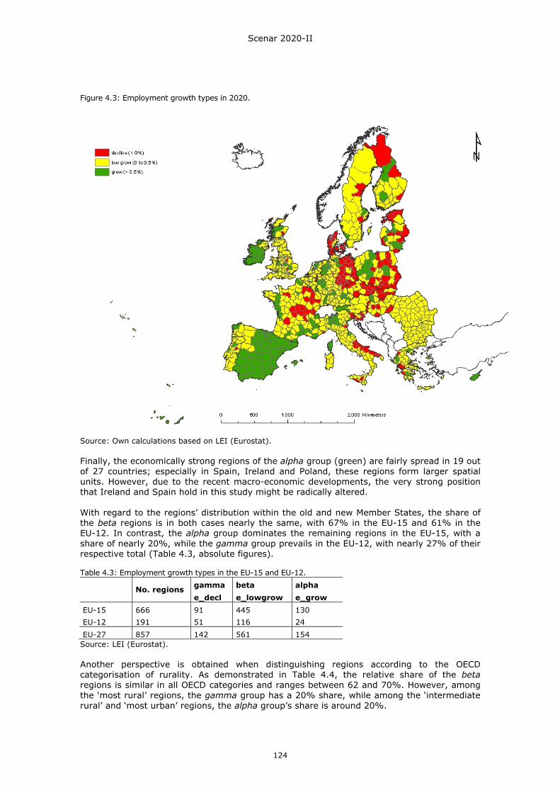
Scenar 2020-II

124

Figure 4.3: Employment growth types in 2020.

Source: Own calculations based on LEI (Eurostat). Finally, the economically strong regions of the alpha group (green) are fairly spread in 19 out of 27 countries; especially in Spain, Ireland and Poland, these regions form larger spatial units. However, due to the recent macro-economic developments, the very strong position that Ireland and Spain hold in this study might be radically altered. With regard to the regions’ distribution within the old and new Member States, the share of the beta regions is in both cases nearly the same, with 67% in the EU-15 and 61% in the EU-12. In contrast, the alpha group dominates the remaining regions in the EU-15, with a share of nearly 20%, while the gamma group prevails in the EU-12, with nearly 27% of their respective total (Table 4.3, absolute figures). Table 4.3: Employment growth types in the EU-15 and EU-12.

gamma beta alpha

No. regions

e_decl e_lowgrow e_grow

EU-15 666 91 445 130 EU-12 191 51 116 24

EU-27 857 142 561 154 Source: LEI (Eurostat). Another perspective is obtained when distinguishing regions according to the OECD categorisation of rurality. As demonstrated in Table 4.4, the relative share of the beta regions is similar in all OECD categories and ranges between 62 and 70%. However, among the ‘most rural’ regions, the gamma group has a 20% share, while among the ‘intermediate rural’ and ‘most urban’ regions, the alpha group’s share is around 20%.

Scenar 2020-II

125

Table 4.4: Employment growth types according to the OECD rurality types.

gamma beta alpha

% of regions % % %

most rural 42 20 66 14 intermediate rural 34 16 62 22 most urban 24 11 70 19

Total 100 17 65 18 Source: Own calculations based on LEI (Eurostat). This brief overview of the projected employment situation reveals that the overall economic trends are slightly positive. There is no clear indication that rural regions are generally in a disadvantaged position as they are represented in all types of regions. However, note that this conclusion is based on past trends. 4.2.2.2. Agricultural employment

With the objective of further characterising the role of agriculture for the regions, the share of agricultural employment has been chosen as a second indicator for economic dynamics. Actually, this indicator stands for two aspects: on the one hand, the economic transformation towards a ‘service and knowledge society’ is expressed by the share of the third sector in both terms of employment and gross value added (GVA), and the quick appraisal says ‘the higher the service sector share, the more “developed” the regional economy’. In this context, a high share of agricultural employment stands for a somehow ‘backward’ region. On the other hand, the share of the regional employment in the agricultural sector also stands for the region’s agricultural vocation, and hence the share of agricultural employment reveals the contribution that the agricultural sector makes to overall employment in terms of working force (actually the indicator available is employment in the primary sector, because in addition to agricultural labour it also includes forestry, fishing and hunting). With regard to the objective of the Scenar 2020-II study, this indicator designates the regions which are likely to react more strongly to global agricultural markets and to agri-policy drivers. Therefore, it is in this double sense that the variable will be interpreted in the following. In 2004, the median share of agricultural employment in the EU-27 was 5.43% and the 75 percentile around 13%. Both figures are clearly shaped by the high primary sector shares in the new accession countries. Projections for the 2020 databases are executed in a similar way as the employment growth rate projections. These calculations result in a median share of 3.05% and a 75 percentile of 7.45% - hereby revealing the general decrease of the sector’s contribution to employment. Most regions with a strong decline of the share (i.e. > 10 basis points) are located in the EU-12, while in the EU-15 there are only 25 out of 570 regions with this case, mostly to be found in Greece. On the other hand, 114 out of the total 857 regions show a certain increase in the sector’s employment. Of these regions, those that show the strongest increases are located in Spain and Bulgaria. The regional distribution of the projected share of agricultural employment is presented in Figure 4.4, where group 1 encompasses all regions with an agricultural employment share below 3.05%, group 2 those with a share between 3.05 and 7.45%, and group 3 comprises the most agriculturally shaped regions with a share of more than 7.45% agricultural employment.

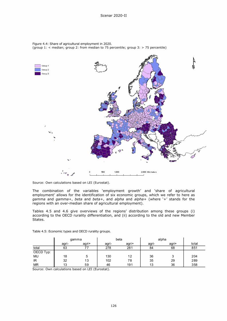
Scenar 2020-II

126

Figure 4.4: Share of agricultural employment in 2020. (group 1: < median; group 2: from median to 75 percentile; group 3: > 75 percentile)

Source: Own calculations based on LEI (Eurostat). The combination of the variables ‘employment growth’ and ‘share of agricultural employment’ allows for the identification of six economic groups, which we refer to here as gamma and gamma+, beta and beta+, and alpha and alpha+ (where ‘+’ stands for the regions with an over-median share of agricultural employment). Tables 4.5 and 4.6 give overviews of the regions’ distribution among these groups (i) according to the OECD rurality differentiation, and (ii) according to the old and new Member States. Table 4.5: Economic types and OECD rurality groups.

agri- agri+ agri- agri+ agri- agri+ totaltotal 63 77 278 281 84 68 851OECD Typ:MU 18 5 130 12 36 3 204IR 32 13 102 78 35 29 289MR 13 59 46 191 13 36 358

alphagamma beta

Source: Own calculations based on LEI (Eurostat).

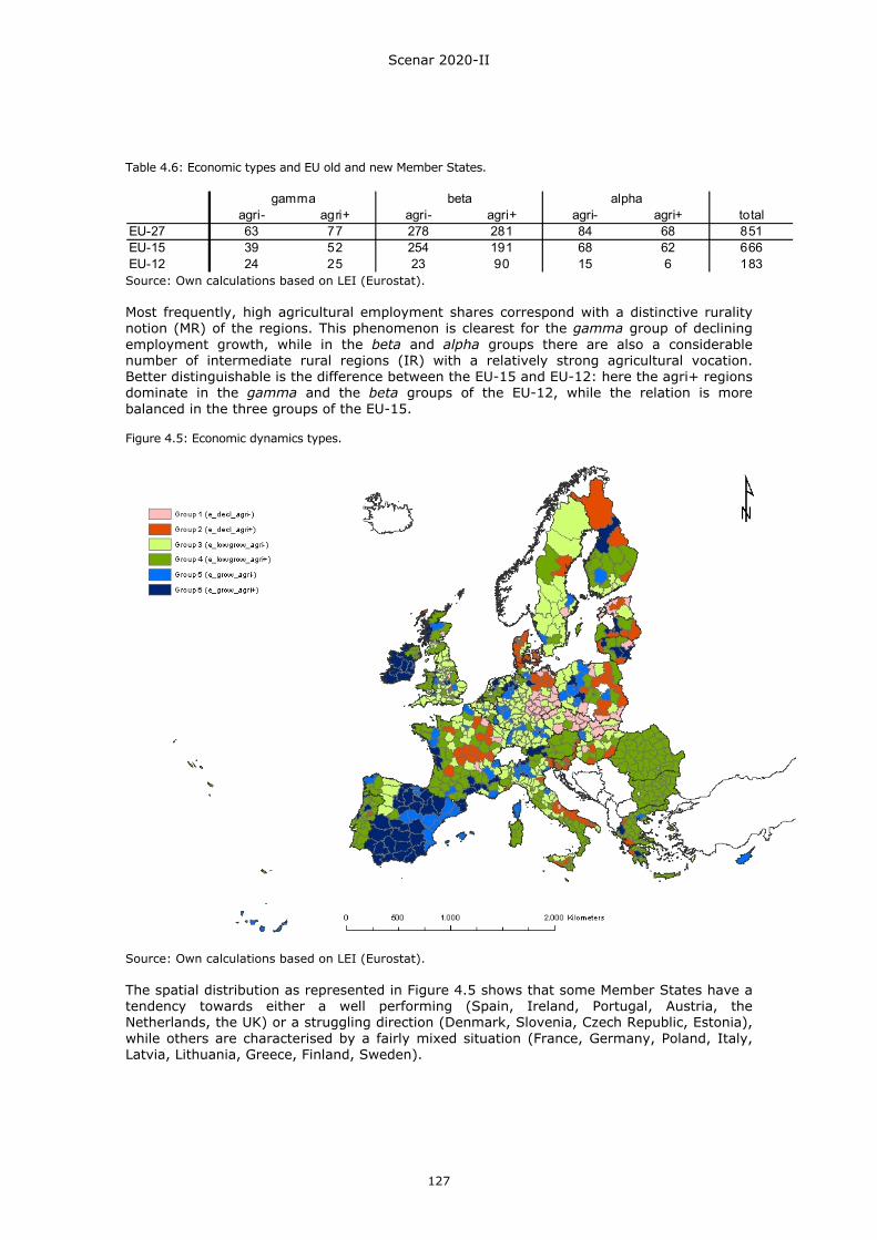
Scenar 2020-II

127

Table 4.6: Economic types and EU old and new Member States.

agri- agri+ agri- agri+ agri- agri+ totalEU-27 63 77 278 281 84 68 851EU-15 39 52 254 191 68 62 666EU-12 24 25 23 90 15 6 183

gamma beta alpha

Source: Own calculations based on LEI (Eurostat). Most frequently, high agricultural employment shares correspond with a distinctive rurality notion (MR) of the regions. This phenomenon is clearest for the gamma group of declining employment growth, while in the beta and alpha groups there are also a considerable number of intermediate rural regions (IR) with a relatively strong agricultural vocation. Better distinguishable is the difference between the EU-15 and EU-12: here the agri+ regions dominate in the gamma and the beta groups of the EU-12, while the relation is more balanced in the three groups of the EU-15. Figure 4.5: Economic dynamics types.

Source: Own calculations based on LEI (Eurostat). The spatial distribution as represented in Figure 4.5 shows that some Member States have a tendency towards either a well performing (Spain, Ireland, Portugal, Austria, the Netherlands, the UK) or a struggling direction (Denmark, Slovenia, Czech Republic, Estonia), while others are characterised by a fairly mixed situation (France, Germany, Poland, Italy, Latvia, Lithuania, Greece, Finland, Sweden).

Scenar 2020-II

128

4.2.3. Typology of socio-economic perspectives The choice of the demographic indicator, on the one hand, and the agri-economic indicators, on the other hand, takes place with the conceptual assumption that demographic development and the employment trend are crucial characteristics for the performance of a region in so far as they can be mutually enforcing or weakening. This interdependency between ‘jobs and people’ is controversially discussed in the literature. It could be assumed that there is a relation between employment growth and population growth: in a study on employment dynamics in rural regions in the EU in the 1980s, it appeared that regions with an above average employment growth also had an above average population growth (Terluin, 2003). Usually, this population growth was partially due to in-migration. Within urban and regional science there is a longstanding debate on the classic question of whether ‘jobs follow people’ or ‘people follow jobs’. A meta-analysis of 308 study results on the relationship of changes in employment and population revealed that empirical evidence is highly inconclusive on whether ‘jobs follow people’ or ‘people follow jobs’ (Hoogstra et al., 2005). Although the hypothesis ‘jobs follow people’ was supported by empirical evidence somewhat more often than the hypothesis ‘people follow jobs’, quite a number of studies showed no interaction between employment and population growth or a dual causality. It seems that these findings confirm the popular belief that the relation between employment growth and population growth has the nature of the chicken-and-egg question. Therefore, both regional qualities are considered as either representing a region’s positive development potentials (i.e. its strengths) or as revealing its deficits (i.e. its weaknesses) and as mutually enforcing. The additional characteristic of employment share in the primary sector is seen as the linking variable between agriculture and the overall regional economy. 4.2.3.1. Conceptualising the SWOT analysis for the socio-economic reaction types

In the following, the socio-economic characteristics of the EU-27’s regions will be presented and comparatively analysed. Based on three key indicators only, this approach is, of course, strongly abstracting from reality and hence somewhat simplistic. However, it is based on some predominant phenomena which can be monitored and evaluated for the EU-27 at a relatively high level of disaggregation, and thus shall serve as a meaningful orientation for further inspection. The combination of the four demographic development groups with the six economic dynamic groups results in 24 subgroups (Table 4.7). As the overall grouping for both themes has occurred in a deliberated manner, these groups are somewhat balanced and correspond to ¼ of the total demographic development each and to 1/6 – 2/3 – 1/6 of the total of economic dynamics. The integration of the variable ‘share of agricultural employment’ adds interesting information and significantly differentiates the regional groups. Table 4.7: Socio-economic performance groups.

agri- agri+ agri- agri+ agri- agri+ totalhigh_popdecl 37 30 43 109 6 4 229low_popdecl 18 33 65 48 11 14 189low_popgrowth 4 12 104 74 19 14 227high_popgrowth 4 2 66 50 48 36 206total 63 77 278 281 84 68 851

gamma beta alpha

Source: Own calculations based on LEI (Eurostat). The determination of strengths and weaknesses with regard to this grouping is done following the conceptual scheme presented in Figure 4.6. As opportunities, the general economic development with an increasing GVA in the service sector (see Section 2.1 in deliverable 2.1) can be taken into account. At the same time, global markets evolve, offering new production possibilities, even for the agricultural sector. On the other hand, more competition from non-EU countries is projected, so that increasing imports, e.g. of meat, can be seen as threats. As a consequence of the decreasing agricultural producer prices (Table 3.2, Section 3.5.1), continuous structural adjustments of the sector will be occurring which are considered as another threat to regional employment. Positive demographic and economic reactions for both agri- and agri+ regions (the complete alpha group) are

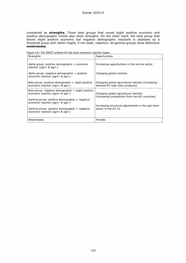
Scenar 2020-II

129

considered as strengths. Those beta groups that reveal slight positive economic and positive demographic trends also show strengths. On the other hand, the beta group that shows slight positive economic but negative demographic reactions is assessed as a threshold group with rather fragile, if not weak, reactions. All gamma groups show distinctive weaknesses. Figure 4.6: The SWOT scheme for the socio-economic reaction types. Strengths Opportunities

Alpha group: positive demographic + economic reaction (agri+ & agri-) Alpha group: negative demographic + positive economic reaction (agri+ & agri-) Beta group: positive demographic + slight positive economic reaction (agri+ & agri-)

Increasing opportunities in the service sector Changing global markets Changing global agricultural markets (increasing demand for high value products)

Beta group: negative demographic + slight positive economic reaction (agri+ & agri-) Gamma group: positive demographic + negative economic reaction (agri+ & agri-) Gamma group: positive demographic + negative economic reaction (agri+ & agri-)

Changing global agricultural markets (increasing competition from non-EU countries) Increasing structural adjustments in the agri-food sector in the EU-12

Weaknesses Threats

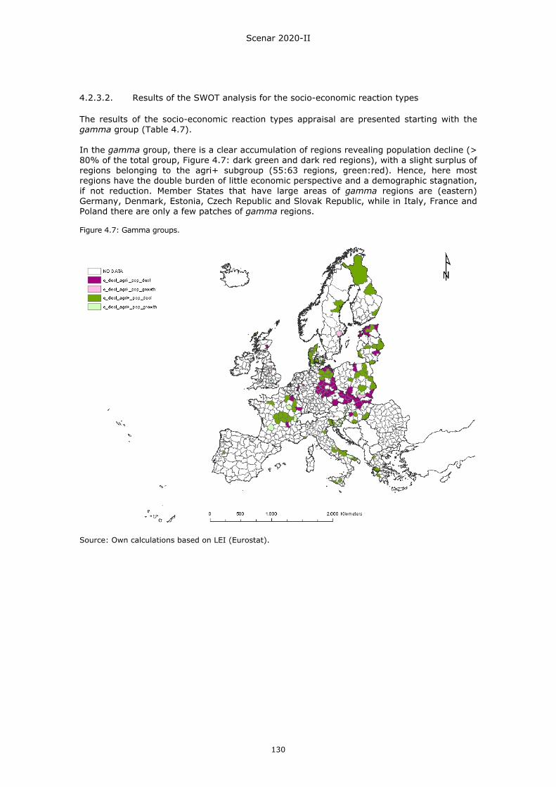
Scenar 2020-II

130

4.2.3.2. Results of the SWOT analysis for the socio-economic reaction types

The results of the socio-economic reaction types appraisal are presented starting with the gamma group (Table 4.7). In the gamma group, there is a clear accumulation of regions revealing population decline (> 80% of the total group, Figure 4.7: dark green and dark red regions), with a slight surplus of regions belonging to the agri+ subgroup (55:63 regions, green:red). Hence, here most regions have the double burden of little economic perspective and a demographic stagnation, if not reduction. Member States that have large areas of gamma regions are (eastern) Germany, Denmark, Estonia, Czech Republic and Slovak Republic, while in Italy, France and Poland there are only a few patches of gamma regions. Figure 4.7: Gamma groups.

Source: Own calculations based on LEI (Eurostat).

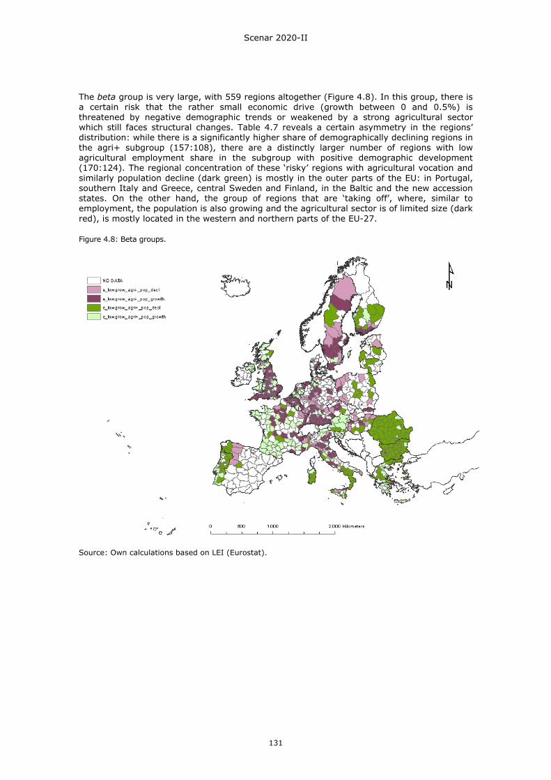
Scenar 2020-II

131

The beta group is very large, with 559 regions altogether (Figure 4.8). In this group, there is a certain risk that the rather small economic drive (growth between 0 and 0.5%) is threatened by negative demographic trends or weakened by a strong agricultural sector which still faces structural changes. Table 4.7 reveals a certain asymmetry in the regions’ distribution: while there is a significantly higher share of demographically declining regions in the agri+ subgroup (157:108), there are a distinctly larger number of regions with low agricultural employment share in the subgroup with positive demographic development (170:124). The regional concentration of these ‘risky’ regions with agricultural vocation and similarly population decline (dark green) is mostly in the outer parts of the EU: in Portugal, southern Italy and Greece, central Sweden and Finland, in the Baltic and the new accession states. On the other hand, the group of regions that are ‘taking off’, where, similar to employment, the population is also growing and the agricultural sector is of limited size (dark red), is mostly located in the western and northern parts of the EU-27.

Figure 4.8: Beta groups.

Source: Own calculations based on LEI (Eurostat).

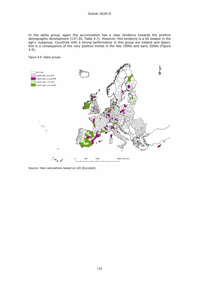
Scenar 2020-II

132

In the alpha group, again the accumulation has a clear tendency towards the positive demographic development (137:35, Table 4.7). However, this tendency is a bit weaker in the agri+ subgroup. Countries with a strong performance in this group are Ireland and Spain; this is a consequence of the very positive trends in the late 1990s and early 2000s (Figure 4.9).

Figure 4.9: Alpha groups.

Source: Own calculations based on LEI (Eurostat).

Scenar 2020-II

133

Looking more closely at the differences between the EU-15 and the EU-12, the numerical relation between the alpha, beta and gamma groups in the EU-15 is 91:445:130. Thus, the beta group corresponds to 2/3 of the total. The gamma and alpha groups are not evenly distributed over the remaining 1/6: the gamma group is distinctly smaller and the alpha group is clearly larger than the remaining 1/6 (Table 4.8). Table 4.8: Socio-economic performance in the EU-15.

agri- agri+ agri- agri+ agri- agri+ totalhigh_popdecl 27 19 30 40 3 2 121low_popdecl 5 23 60 35 6 11 140low_popgrowth 4 9 98 68 15 14 208high_popgrowth 3 1 66 48 44 35 197total 39 52 254 191 68 62 666

gamma beta alpha

Source: Own calculations based on LEI (Eurostat). Table 4.9: Socio-economic performance in the EU-12.

agri- agri+ agri- agri+ agri- agri+ totalhigh_popdecl 10 11 13 69 3 2 108low_popdecl 13 10 5 13 5 3 49low_popgrowth 0 3 6 6 4 0 19high_popgrowth 1 1 0 2 4 1 9total 24 25 24 90 16 6 185

gamma beta alpha

Source: Own calculations based on LEI (Eurostat). In contrast, in the EU-12, the relation is 49:114:22 – which means that the alpha and the beta groups are distinctly smaller than 1/6 and 2/3, while the gamma group has a relatively high share of the total (Table 4.9). Demographically declining regions dominate almost all EU-12 subgroups – a finding that is clearly a sign of a structural weakness of many eastern European regions. Looking more closely at the differentiation between the regions with an above-median and a below-median share of employment in the agricultural sector, it is the subgroup of little employment growth (beta+ popdecl) which, with 82 members, makes up nearly 45% of the EU-12’s total. 4.2.3.3. Conclusions

The general picture of the EU-27 regions’ socio-economic reactions in 2020 is that of fairly small changes. Population growth and decline as well as changes in employment growth range largely between -1 and +1% annual change rate. Hence, without moderating the existing differences too much, a relative stability can be expected. Of course, the impacts of the current economic crisis are not included in the projective calculations and therefore cannot be assessed here. They might lead in some places to the accentuation of negative tendencies and trends. Furthermore, the analysis shows that, although all types of regions are represented all over the EU-27, there is a difference between the EU-12 and the EU-15, with the more positive reactions in the old Member States. Hence, with regard to the opportunities in the service sector, it could be discussed whether emerging ‘strong’ regions and clusters in the EU-12 and in the southern parts of the EU-15 should be enhanced so that they can lead in the structural transformation towards more service orientation in employment. There is no evidence that the EU-27 regions with an above average agricultural employment are generally showing negative reactions. Hence, it shall be emphasised that rurality and agricultural vocation are not a sign of weak development perspectives. However, as the overall trend in the sector’s employment is declining (median drops from 5.43% in 2004 to 3.05% in 2020), it cannot be counted on as a stabilising factor either. Nevertheless, if employment-relevant policy measures are discussed within a rural development framework (as e.g. the third axis and the LEADER programme within the European Agricultural Fund for

Scenar 2020-II

134

Rural Development (EAFRD) Regulation36), then their objectives and possible impacts should be analysed and assessed before the general socio-economic performance of a region.

4.3. Selected structural strengths and weaknesses In order to valorise regional characteristics that cannot easily be projected, selected ‘structural’ characteristics of the EU-27 regions are presented on the basis of current data (2000-2005), namely ‘quality of life’ (Section 4.3.1), ‘environmental preconditions’ (Section 4.3.2) and ‘agri-structural preconditions’ (Section 4.3.3). According to the level of data disaggregation, quality of life and environmental issues can be assessed at the FARO level (857 regions), while the agri-structural information is presented at the HARM2 level (665 regions). Section 4.3 closes with an assessment of the structural strengths and weaknesses as contrasted with the socio-economic developments (Section 4.3.4). The environmental conditions are discussed in contrast to the projected agricultural land use in order to assess regional disposition for vulnerability (Section 4.4.3). 4.3.1. Quality of life appraisal 4.3.1.1. Indicators for approaching quality of life

Quality of life is a broad concept concerned with overall well-being within society. Its aim is to enable people, as far as possible, to achieve their goals and choose their ideal lifestyle (EFILWC, 2004). Defined in this way, the quality of life concept goes beyond an approach directed at material conditions. According to the European Foundation for the Improvement of Living and Working Conditions - EFILWC (2004), three main characteristics can be attributed to the quality of life concept: 1) Quality of life refers to individuals’ life conditions; as such, it is a micro concept. 2) Quality of life is a multidimensional concept: it focuses on several life domains and the

interplay between these domains. 3) Quality of life is measured by both objective and subjective indicators. In 2003, EFILWC conducted a survey on the quality of life in the EU-27 plus Turkey. In the analysis of the quality of life, EFILWC used individual indicators and did not attempt to combine individual indicators into a multidimensional indicator for quality of life. Individual indicators include: household’s total income, number of rooms per person, proportion of households with problems with accommodation, proportion of respondents complaining about environmental problems, persons living in a household with/without job, work-life balance, health situation per income group, access to health services, quality of health and social services, life satisfaction, tensions between social groups, and perceived quality of the education, social benefit and pension system (EFILWC, 2004). The second edition of the survey from the EFILWC was carried out in 2007 and covers all the EU Member States, Norway and the three accession candidate countries (ACCs) Croatia, FYR Macedonia and Turkey. The claim of the first European Quality of Life Survey remains true for the second edition. Comparing the first and second surveys, it seems that the rank ordering of the countries is constant over time (EFILWC, 2009). 4.3.1.2. Quality of life in urban and rural areas

Results of the EFILWC quality of life survey 2003 were reported at Member State level. Later, results were also reported for urban and rural areas; however, this was at a fairly aggregated level for four different groups of countries according to their level of GDP/capita: EU-12 high, EU-7 intermediate; EU-6 low and the – at that time - accession candidates Bulgaria, Romania and Turkey (EFILWC, 2006). The distinction between urban and rural 36 Council Regulation (EC) No. 1698/2005.

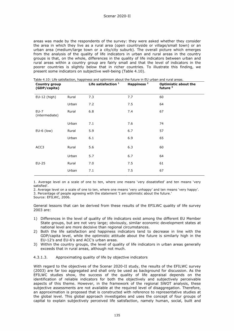
Scenar 2020-II

135

areas was made by the respondents of the survey: they were asked whether they consider the area in which they live as a rural area (open countryside or village/small town) or an urban area (medium/large town or a city/city suburb). The overall picture which emerges from the analysis of the quality of life indicators in urban and rural areas in the country groups is that, on the whole, differences in the quality of life indicators between urban and rural areas within a country group are fairly small and that the level of indicators in the poorer countries is slightly below that in richer countries. To illustrate this finding, we present some indicators on subjective well-being (Table 4.10). Table 4.10: Life satisfaction, happiness and optimism about the future in EU urban and rural areas. Country group (GDP/capita)

Life satisfaction 1 Happiness 2 Optimistic about the future 3

EU-12 (high) Rural 7.3 7.7 60

Urban 7.2 7.5 64

EU-7 (intermediate)

Rural 6.8 7.4 67

Urban 7.1 7.6 74

EU-6 (low) Rural 5.9 6.7 57

Urban 6.1 6.9 65

ACC3 Rural 5.6 6.3 60

Urban 5.7 6.7 64

EU-25 Rural 7.0 7.5 61

Urban 7.1 7.5 67

1. Average level on a scale of one to ten, where one means ‘very dissatisfied’ and ten means ‘very satisfied’. 2. Average level on a scale of one to ten, where one means ‘very unhappy’ and ten means ‘very happy’. 3. Percentage of people agreeing with the statement ‘I am optimistic about the future.’ Source: EFILWC, 2006. General lessons that can be derived from these results of the EFILWC quality of life survey 2003 are: 1) Differences in the level of quality of life indicators exist among the different EU Member

State groups, but are not very large; obviously, similar economic development states at national level are more decisive than regional circumstances.

2) Both the life satisfaction and happiness indicators tend to decrease in line with the GDP/capita level, while the optimistic attitude about the future is similarly high in the EU-12’s and EU-6’s and ACC’s urban areas.

3) Within the country groups, the level of quality of life indicators in urban areas generally exceeds that in rural areas, although not much.

4.3.1.3. Approximating quality of life by objective indicators

With regard to the objectives of the Scenar 2020-II study, the results of the EFILWC survey (2003) are far too aggregated and shall only be used as background for discussion. As the EFILWC studies show, the success of the quality of life appraisal depends on the identification of reliable indicators for both the objectively and subjectively perceivable aspects of this theme. However, in the framework of the regional SWOT analysis, these subjective assessments are not available at the required level of disaggregation. Therefore, an approximation is proposed that is constructed with reference to representative studies at the global level. This global approach investigates and uses the concept of four groups of capital to explain subjectively perceived life satisfaction, namely human, social, built and

Scenar 2020-II

136

natural capital (Vemuri & Costanza, 2006). Here, human capital is characterised with the help of the UN Human Development Index (HDI), which is composed of a longevity index, an education index and the standard living index which refers to capital income per capita. Natural capital is represented by the ‘ecosystem services product’, a land-cover based monetary estimation of the total value of ecosystem services per country (Costanza et al., 1997). Finally, social capital was best identified by the proxy index ‘freedom of the press’ which, however, correlates highly with both the human and built capital as well as with the natural capital. The study showed that the indices for human and built capital, on the one hand, and for natural capital, on the other, were able to explain 72% of the variation in life satisfaction in 171 countries. The authors emphasise the importance of the natural capital variable for the explanation of subjective well-being, a variable that is not intercorrelated with any other of the explanatory factors and stands for a direct linkage between people’s well-being and the natural assets of a country. Nevertheless, human and built capital as captured by the HDI is the most important explanatory factor, in particular income or material welfare, but also the realisation of basic biological and social needs (Vemuri & Costanza, 2006). 4.3.1.4. Measuring quality of life at regional level

Following the ‘capital approach’ described above, an adaptation for the Scenar 2020-II SWOT appraisal was developed that is based on indicators available for the EU-27 regions at FARO level. Initially, all four capital types should be represented by selected appropriate variables. On the basis of the UN HDI index, indicators for human and built capital should be selected. However, the educational and life expectation indicators are only available at NUTS 1 or 2 in the EU-27, whereas GDP/capita can be obtained even at NUTS3. Therefore, the indicator GDP/capita is used to represent built capital. Actually, GDP/capita has a long tradition as a measurement for well-being; however, it has been widely criticised because (i) it is a purely material figure, (ii) it does not reflect income distribution, and (iii) taxes and income transfers are also omitted (Stewart, 2002; Frick & Grabka, 2009). As an approximation to both human and social capital, the availability of and access to multifold services, such as education, health care, a free press and open information, etc., were chosen, based on plausibility considerations. The variable chosen to represent this capital is the regional share of the service sector in terms of GVA. This indicator stands for the region’s potential to access to all sorts of services for its inhabitants. Finally, in order to take the natural capital into account, the ‘Green Background Landscape Index (GBLI)’ is used, a new variable that is explained in more detail in the following paragraph. Excursus: The Green Background Landscape Index (GBLI)

The GBLI indicates landscape characteristics favourable to nature. The Green Background Landscape can be seen as a natural asset on its own as well as an important component (with rivers) of the connectivity between areas of high ecological interest. The GBLI is mapped from a selection of aggregated Corine Land Cover (CLC) classes smoothed in order to compute their value in their neighbourhood (Britz et al., 2007). The methodology is presented in Land accounts for Europe 1990-2000 (EEA, 2006). The standard map (Figure 4.10) is based on CLC classes 2B, 3, 4 and 5, namely: 1) C2B: Pastures and mosaic farmland. 2) C3A: Forests and transitional woodland shrub. 3) C3B: Natural grassland, heathland, sclerophylous vegetation. 4) C3C: Open space with little or no vegetation. 5) C4: Wetlands. 6) C5: Water bodies. These categories were chosen because agro-systems with pastures and/or mosaics of parcels, forests and other semi-natural or natural drylands, wetlands and water bodies are land cover types a priori favourable to nature, independently from their designation or protection status.

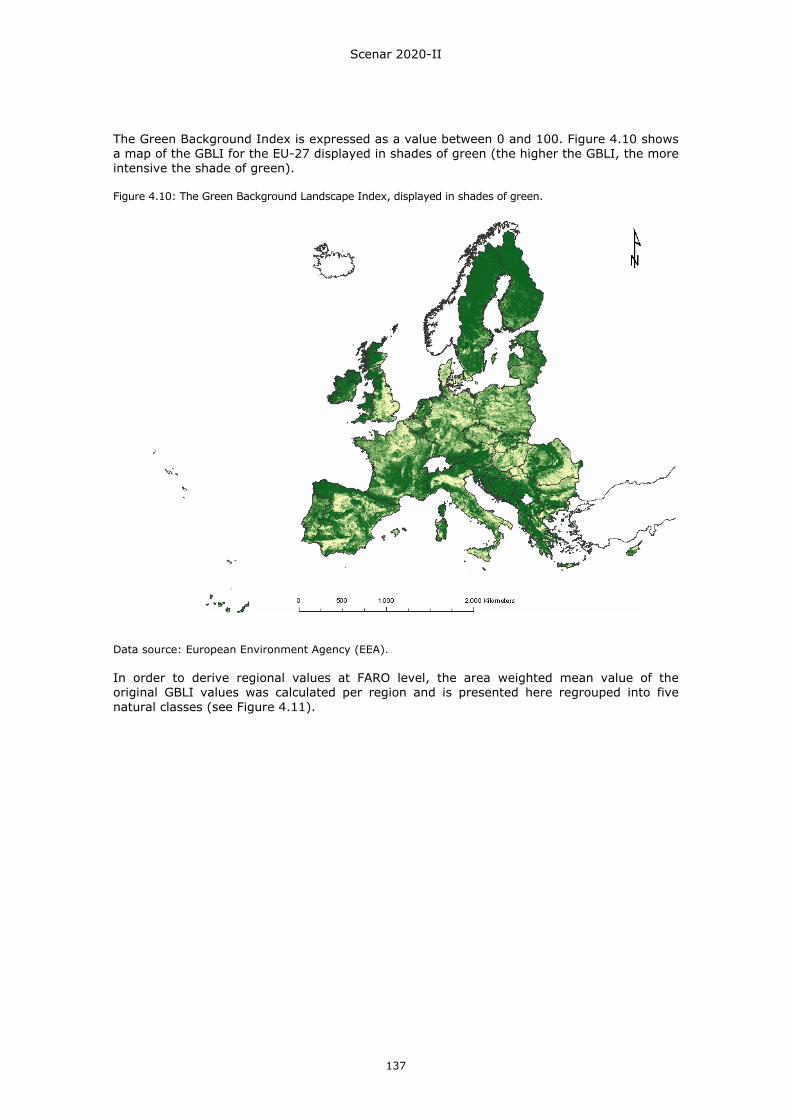
Scenar 2020-II

137

The Green Background Index is expressed as a value between 0 and 100. Figure 4.10 shows a map of the GBLI for the EU-27 displayed in shades of green (the higher the GBLI, the more intensive the shade of green). Figure 4.10: The Green Background Landscape Index, displayed in shades of green.

Data source: European Environment Agency (EEA). In order to derive regional values at FARO level, the area weighted mean value of the original GBLI values was calculated per region and is presented here regrouped into five natural classes (see Figure 4.11).

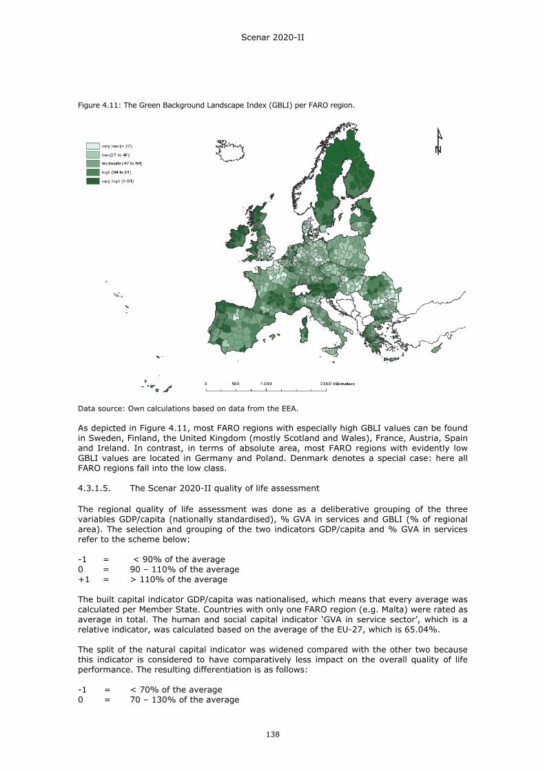
Scenar 2020-II

138

Figure 4.11: The Green Background Landscape Index (GBLI) per FARO region.

Data source: Own calculations based on data from the EEA. As depicted in Figure 4.11, most FARO regions with especially high GBLI values can be found in Sweden, Finland, the United Kingdom (mostly Scotland and Wales), France, Austria, Spain and Ireland. In contrast, in terms of absolute area, most FARO regions with evidently low GBLI values are located in Germany and Poland. Denmark denotes a special case: here all FARO regions fall into the low class. 4.3.1.5. The Scenar 2020-II quality of life assessment

The regional quality of life assessment was done as a deliberative grouping of the three variables GDP/capita (nationally standardised), % GVA in services and GBLI (% of regional area). The selection and grouping of the two indicators GDP/capita and % GVA in services refer to the scheme below: -1 = < 90% of the average 0 = 90 – 110% of the average +1 = > 110% of the average The built capital indicator GDP/capita was nationalised, which means that every average was calculated per Member State. Countries with only one FARO region (e.g. Malta) were rated as average in total. The human and social capital indicator ‘GVA in service sector’, which is a relative indicator, was calculated based on the average of the EU-27, which is 65.04%. The split of the natural capital indicator was widened compared with the other two because this indicator is considered to have comparatively less impact on the overall quality of life performance. The resulting differentiation is as follows: -1 = < 70% of the average 0 = 70 – 130% of the average

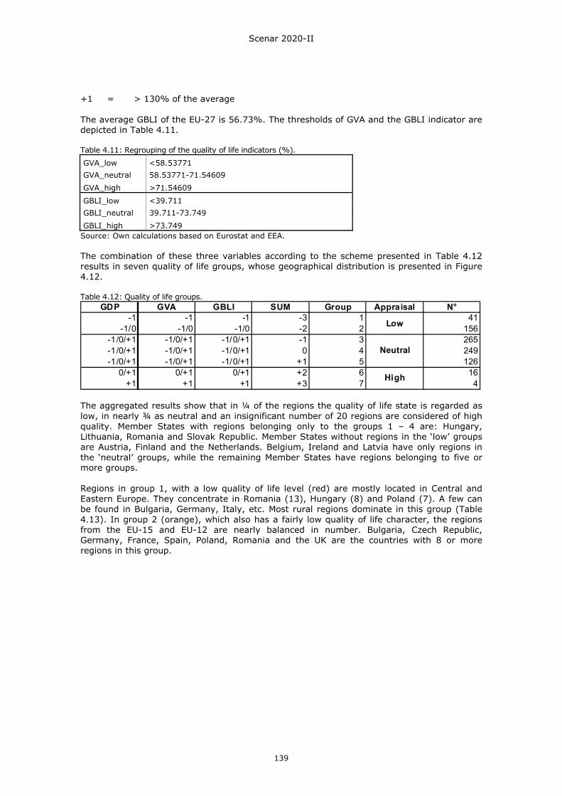
Scenar 2020-II

139

+1 = > 130% of the average The average GBLI of the EU-27 is 56.73%. The thresholds of GVA and the GBLI indicator are depicted in Table 4.11. Table 4.11: Regrouping of the quality of life indicators (%).

GVA_low <58.53771 GVA_neutral 58.53771-71.54609

GVA_high >71.54609

GBLI_low <39.711 GBLI_neutral 39.711-73.749

GBLI_high >73.749 Source: Own calculations based on Eurostat and EEA. The combination of these three variables according to the scheme presented in Table 4.12 results in seven quality of life groups, whose geographical distribution is presented in Figure 4.12. Table 4.12: Quality of life groups.

GDP GVA GBLI SUM Group Appraisal N°-1 -1 -1 -3 1 41

-1/0 -1/0 -1/0 -2 2 156-1/0/+1 -1/0/+1 -1/0/+1 -1 3 265-1/0/+1 -1/0/+1 -1/0/+1 0 4 249-1/0/+1 -1/0/+1 -1/0/+1 +1 5 126

0/+1 0/+1 0/+1 +2 6 16+1 +1 +1 +3 7 4

Low

Neutral

High

The aggregated results show that in ¼ of the regions the quality of life state is regarded as low, in nearly ¾ as neutral and an insignificant number of 20 regions are considered of high quality. Member States with regions belonging only to the groups 1 – 4 are: Hungary, Lithuania, Romania and Slovak Republic. Member States without regions in the ‘low’ groups are Austria, Finland and the Netherlands. Belgium, Ireland and Latvia have only regions in the ‘neutral’ groups, while the remaining Member States have regions belonging to five or more groups. Regions in group 1, with a low quality of life level (red) are mostly located in Central and Eastern Europe. They concentrate in Romania (13), Hungary (8) and Poland (7). A few can be found in Bulgaria, Germany, Italy, etc. Most rural regions dominate in this group (Table 4.13). In group 2 (orange), which also has a fairly low quality of life character, the regions from the EU-15 and EU-12 are nearly balanced in number. Bulgaria, Czech Republic, Germany, France, Spain, Poland, Romania and the UK are the countries with 8 or more regions in this group.

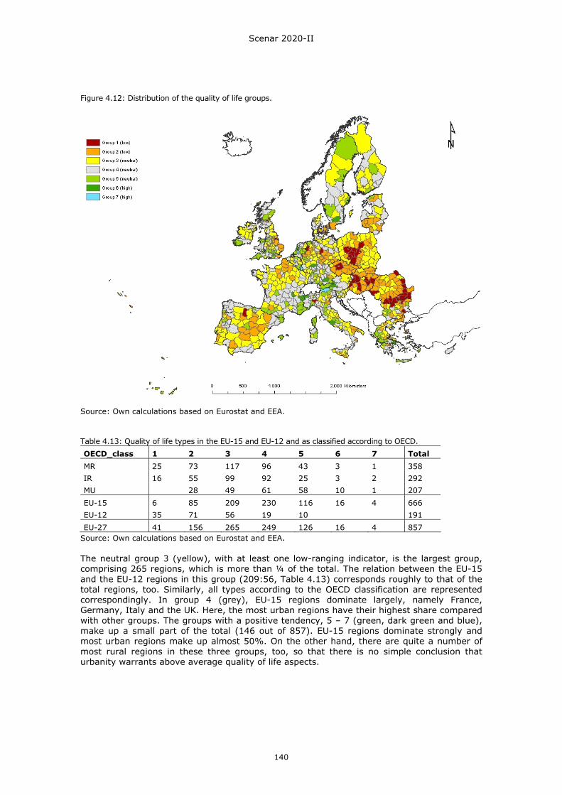
Scenar 2020-II

140

Figure 4.12: Distribution of the quality of life groups.

Source: Own calculations based on Eurostat and EEA. Table 4.13: Quality of life types in the EU-15 and EU-12 and as classified according to OECD.

OECD_class 1 2 3 4 5 6 7 Total

MR 25 73 117 96 43 3 1 358 IR 16 55 99 92 25 3 2 292 MU 28 49 61 58 10 1 207

EU-15 6 85 209 230 116 16 4 666 EU-12 35 71 56 19 10 191

EU-27 41 156 265 249 126 16 4 857 Source: Own calculations based on Eurostat and EEA. The neutral group 3 (yellow), with at least one low-ranging indicator, is the largest group, comprising 265 regions, which is more than ¼ of the total. The relation between the EU-15 and the EU-12 regions in this group (209:56, Table 4.13) corresponds roughly to that of the total regions, too. Similarly, all types according to the OECD classification are represented correspondingly. In group 4 (grey), EU-15 regions dominate largely, namely France, Germany, Italy and the UK. Here, the most urban regions have their highest share compared with other groups. The groups with a positive tendency, 5 – 7 (green, dark green and blue), make up a small part of the total (146 out of 857). EU-15 regions dominate strongly and most urban regions make up almost 50%. On the other hand, there are quite a number of most rural regions in these three groups, too, so that there is no simple conclusion that urbanity warrants above average quality of life aspects.

Scenar 2020-II

141

4.3.2. Environmental preconditions As for other factors, regional environmental conditions can be understood as strengths (in terms of ecological assets) and weaknesses (i.e. specific environmental vulnerabilities) for regional development in general and the agricultural sector in particular. In Scenar 2020-II, four environmental topics are considered to characterise the environmental preconditions at regional level: soil characteristics and water issues, soil degradation issues, soil-related greenhouse gas (GHG) emission, and areas important for biodiversity issues. The selection of indicators sets the focus on those issues that possibly represent an environmental vulnerability with regard to agricultural land use. Similarly, restrictions in data availability had to be dealt with. In the case of climate change-relevant GHG, only the environmental opportunity of contribution to mitigation is discussed. For each of these topics one or several indicators were taken into account: Soil characteristics and water issues: • Share of area with low subsoil and/or topsoil water availability • Share of area with permeable (sandy) soils and groundwater pollution. Soil degradation issues: • Share of soils sensitive to erosion. Soil–related greenhouse gas emissions: • Share of soils rich in soil organic matter • Share of organic soils under agricultural management • Share of structural land-use changes (CLC based) with impact on soil organic carbon • Share of low organic content soils under agricultural management. Areas important for biodiversity issues: • Share of Natura 2000 areas • Share of High Nature Value (HNV) farmland area. In the following sections, a short passage is dedicated to each topic and its chosen indicators, describing why this topic was chosen and how the single risk map per indicator at FARO level was derived. 4.3.2.1. Soil water issues: subsoil and topsoil water availability

Soil water availability for plants is one of the main drivers for soil fertility and for the usage of soils for agricultural production. Plant available water is considered to be the water held in soils between field capacity and wilting point. However, different plant species possess different abilities to take up water from topsoil and subsoil layers depending on their root depth and root-system architecture. Generally, soils that show a restricted water availability offer only a limited capability for farmland usage. If they are nevertheless used for agricultural production, they are dependent on irrigation systems for additional water supply to nurse plants. If water balance allows this, there is no problem. If not, such systems are not sustainable. The problem of water shortage will become more important in the future against the background of climate change (Rockstrom et al., 2009; see also Figure 4.14). The information on subsoil and topsoil available water capacity was obtained from the European Soil Database (ESDB). As data on soil characteristics and properties are delivered by the single member countries, data quality may vary between countries (Daroussin & King, 2009). Furthermore, yearly average rainfall and temperature could not be included in the analysis. The calculation of the ESDB was derived from so-called ‘pedo-transfer functions’ built on expert knowledge of soil experts (Bouma & Van Lanen, 1986). Available water capacities were calculated for the different topsoil and subsoil horizons of the Soil Geographical Database (King et al., 1994) characterised by its topsoil and subsoil textures and the packing density. Next, the amount of water was multiplied by the thickness of each horizon to obtain the available amount of water (Daroussin & King, 2009; Wösten, 2009).

Scenar 2020-II

142

Based on the ESDB data the map in Figure 4.13 was derived, highlighting those regions where restricted subsoil or topsoil water capacity is deemed to be a limiting factor for agricultural production. For calculating the share of soils per FARO region with limited water availability in soils the classes ‘very low’ (available water capacity equals 0 mm/m) and ‘low’ (available water capacity is lower than 100 mm/m) were taken into account. Figure 4.13: Share of soils with low or very low subsoil and topsoil available water capacity (%).

Data source: Own calculations based on data from the European Soil Database (ESDB). The grouping into five classes was done by applying the natural breaks classification scheme following Jenks. As shown in Figure 4.13 most FARO regions showing a very high share (> 46%) of soils with limited water availability are located in southern Europe in Spain and Greece but some also in Central and Eastern Europe in parts of Austria, Slovenia and Bulgaria. However, as soil properties are important but not the only driver of soil water availability, a more complete picture with respect to limited water availability can be drawn when yearly rainfall and temperatures are included in the assessment. As an example, Figure 4.14 gives additional information on those regions where rainfall has decreased in the last five decades (1960-2006) tightening the problem of water scarcity.

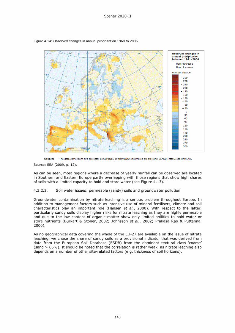
Scenar 2020-II

143

Figure 4.14: Observed changes in annual precipitation 1960 to 2006.

Source: EEA (2009, p. 12). As can be seen, most regions where a decrease of yearly rainfall can be observed are located in Southern and Eastern Europe partly overlapping with those regions that show high shares of soils with a limited capacity to hold and store water (see Figure 4.13). 4.3.2.2. Soil water issues: permeable (sandy) soils and groundwater pollution

Groundwater contamination by nitrate leaching is a serious problem throughout Europe. In addition to management factors such as intensive use of mineral fertilisers, climate and soil characteristics play an important role (Hansen et al., 2000). With respect to the latter, particularly sandy soils display higher risks for nitrate leaching as they are highly permeable and due to the low content of organic matter show only limited abilities to hold water or store nutrients (Burkart & Stoner, 2002; Johnsson et al., 2002; Prakasa Rao & Puttanna, 2000). As no geographical data covering the whole of the EU-27 are available on the issue of nitrate leaching, we chose the share of sandy soils as a provisional indicator that was derived from data from the European Soil Database (ESDB) from the dominant textural class ‘coarse’ (sand > 65%). It should be noted that the correlation is rather weak, as nitrate leaching also depends on a number of other site-related factors (e.g. thickness of soil horizons).

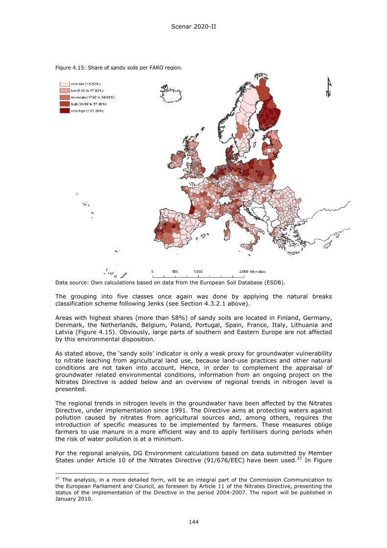
Scenar 2020-II

144

Figure 4.15: Share of sandy soils per FARO region.

Data source: Own calculations based on data from the European Soil Database (ESDB). The grouping into five classes once again was done by applying the natural breaks classification scheme following Jenks (see Section 4.3.2.1 above). Areas with highest shares (more than 58%) of sandy soils are located in Finland, Germany, Denmark, the Netherlands, Belgium, Poland, Portugal, Spain, France, Italy, Lithuania and Latvia (Figure 4.15). Obviously, large parts of southern and Eastern Europe are not affected by this environmental disposition. As stated above, the ‘sandy soils’ indicator is only a weak proxy for groundwater vulnerability to nitrate leaching from agricultural land use, because land-use practices and other natural conditions are not taken into account. Hence, in order to complement the appraisal of groundwater related environmental conditions, information from an ongoing project on the Nitrates Directive is added below and an overview of regional trends in nitrogen level is presented. The regional trends in nitrogen levels in the groundwater have been affected by the Nitrates Directive, under implementation since 1991. The Directive aims at protecting waters against pollution caused by nitrates from agricultural sources and, among others, requires the introduction of specific measures to be implemented by farmers. These measures oblige farmers to use manure in a more efficient way and to apply fertilisers during periods when the risk of water pollution is at a minimum. For the regional analysis, DG Environment calculations based on data submitted by Member States under Article 10 of the Nitrates Directive (91/676/EEC) have been used.37 In Figure

37 The analysis, in a more detailed form, will be an integral part of the Commission Communication to the European Parliament and Council, as foreseen by Article 11 of the Nitrates Directive, presenting the status of the implementation of the Directive in the period 2004-2007. The report will be published in January 2010.

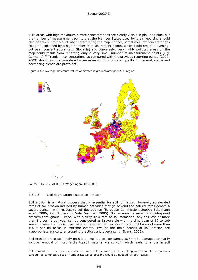
Scenar 2020-II

145

4.16 areas with high maximum nitrate concentrations are clearly visible in pink and blue, but the number of measurement points that the Member States used for their reporting should also be taken into account when interpreting the map. In fact, sometimes low concentrations could be explained by a high number of measurement points, which could result in evening-out peak concentrations (e.g. Slovakia) and conversely, very highly polluted areas on the map could result from reporting only a very small number of measurement points (e.g. Germany).38 Trends in concentrations as compared with the previous reporting period (2000-2003) should also be considered when assessing groundwater quality. In general, stable and decreasing trends are prevalent. Figure 4.16: Average maximum values of nitrates in groundwater per FARO region.

0-2526 - 4041 - 5051 - 100101 - 400

Average Maximum Values NO3 in Groundwater per NUTS FARO (mg/l)

Source: DG ENV, ALTERRA Wageningen, JRC, 2009. 4.3.2.3. Soil degradation issues: soil erosion

Soil erosion is a natural process that is essential for soil formation. However, accelerated rates of soil erosion induced by human activities that go beyond the natural rates denote a severe concern with respect to soil degradation (European Commission, 2009b; Eckelmann et al., 2006; Paz Gonzalez & Vidal Vazquez, 2005). Soil erosion by water is a widespread problem throughout Europe. With a very slow rate of soil formation, any soil loss of more than 1 t per ha per year can be considered as irreversible within a time span of 50 to 100 years. Losses of 20 to 40 t per ha are measured regularly in Europe. Soil losses of more than 100 t per ha occur in extreme events. Two of the main causes of soil erosion are inappropriate agricultural cropping practices and overgrazing (Evans, 2005). Soil erosion processes imply on-site as well as off-site damages. On-site damages primarily include removal of most fertile topsoil material via run-off, which leads to a loss in soil

38 Comment: In order for the reader to interpret the map correctly taking into account the previous caveats, as complete a list of Member States as possible would be needed for both cases.

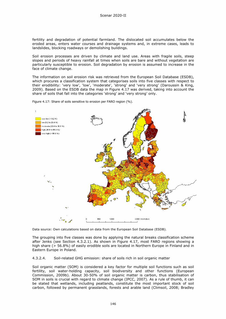
Scenar 2020-II

146

fertility and degradation of potential farmland. The dislocated soil accumulates below the eroded areas, enters water courses and drainage systems and, in extreme cases, leads to landslides, blocking roadways or demolishing buildings. Soil erosion processes are driven by climate and land use. Areas with fragile soils, steep slopes and periods of heavy rainfall at times when soils are bare and without vegetation are particularly susceptible to erosion. Soil degradation by erosion is assumed to increase in the face of climate change. The information on soil erosion risk was retrieved from the European Soil Database (ESDB), which procures a classification system that categorises soils into five classes with respect to their erodibility: ‘very low’, ‘low’, ‘moderate’, ‘strong’ and ‘very strong’ (Daroussin & King, 2009). Based on the ESDB data the map in Figure 4.17 was derived, taking into account the share of soils that fall into the categories ‘strong’ and ‘very strong’ only. Figure 4.17: Share of soils sensitive to erosion per FARO region (%).

Data source: Own calculations based on data from the European Soil Database (ESDB). The grouping into five classes was done by applying the natural breaks classification scheme after Jenks (see Section 4.3.2.1). As shown in Figure 4.17, most FARO regions showing a high share (> 56.8%) of easily erodible soils are located in Northern Europe in Finland and in Eastern Europe in Poland. 4.3.2.4. Soil-related GHG emission: share of soils rich in soil organic matter

Soil organic matter (SOM) is considered a key factor for multiple soil functions such as soil fertility, soil water-holding capacity, soil biodiversity and other functions (European Commission, 2009b). About 30-50% of soil organic matter is carbon, thus stabilisation of SOM in soils is crucial with regard to climate change (IPCC, 2007). As a rule of thumb, it can be stated that wetlands, including peatlands, constitute the most important stock of soil carbon, followed by permanent grasslands, forests and arable land (Climsoil, 2008; Bradley

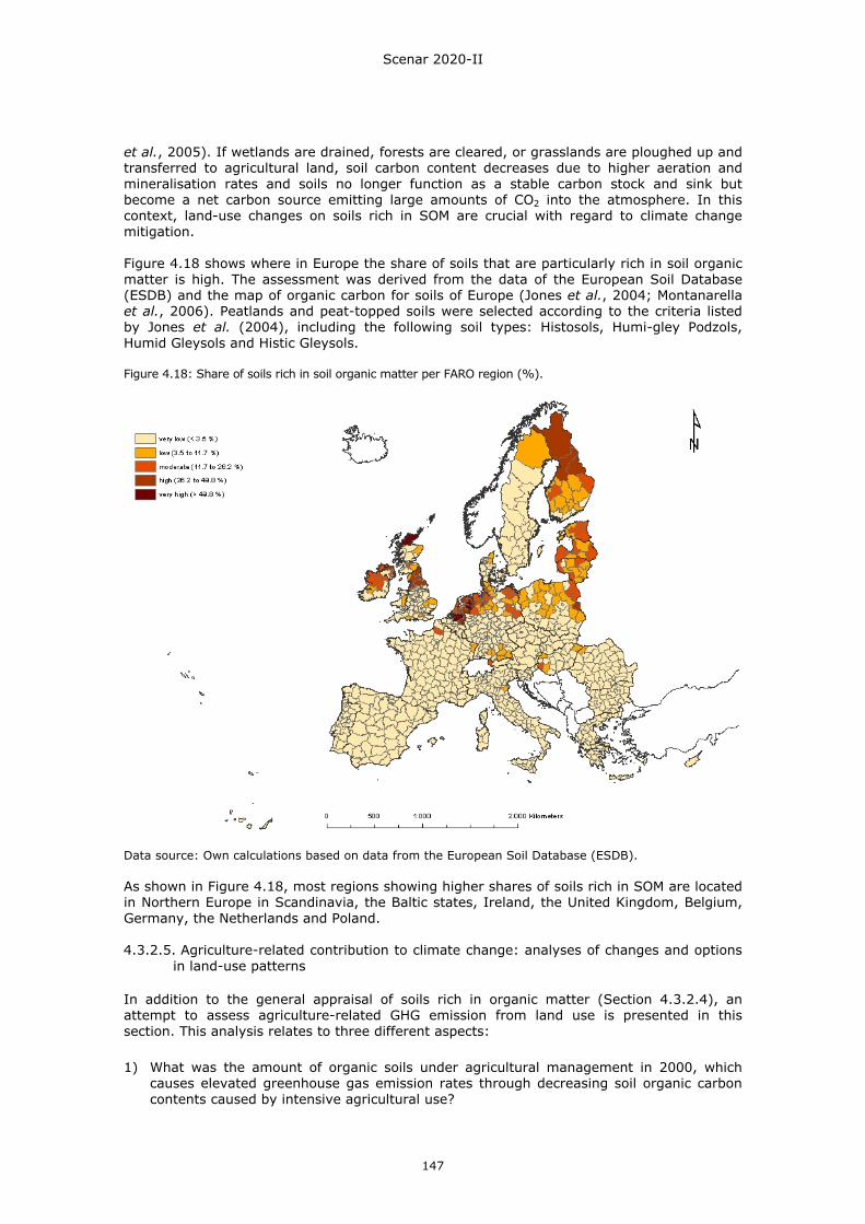
Scenar 2020-II

147

et al., 2005). If wetlands are drained, forests are cleared, or grasslands are ploughed up and transferred to agricultural land, soil carbon content decreases due to higher aeration and mineralisation rates and soils no longer function as a stable carbon stock and sink but become a net carbon source emitting large amounts of CO2 into the atmosphere. In this context, land-use changes on soils rich in SOM are crucial with regard to climate change mitigation. Figure 4.18 shows where in Europe the share of soils that are particularly rich in soil organic matter is high. The assessment was derived from the data of the European Soil Database (ESDB) and the map of organic carbon for soils of Europe (Jones et al., 2004; Montanarella et al., 2006). Peatlands and peat-topped soils were selected according to the criteria listed by Jones et al. (2004), including the following soil types: Histosols, Humi-gley Podzols, Humid Gleysols and Histic Gleysols. Figure 4.18: Share of soils rich in soil organic matter per FARO region (%).

Data source: Own calculations based on data from the European Soil Database (ESDB). As shown in Figure 4.18, most regions showing higher shares of soils rich in SOM are located in Northern Europe in Scandinavia, the Baltic states, Ireland, the United Kingdom, Belgium, Germany, the Netherlands and Poland. 4.3.2.5. Agriculture-related contribution to climate change: analyses of changes and options

in land-use patterns

In addition to the general appraisal of soils rich in organic matter (Section 4.3.2.4), an attempt to assess agriculture-related GHG emission from land use is presented in this section. This analysis relates to three different aspects: 1) What was the amount of organic soils under agricultural management in 2000, which

causes elevated greenhouse gas emission rates through decreasing soil organic carbon contents caused by intensive agricultural use?

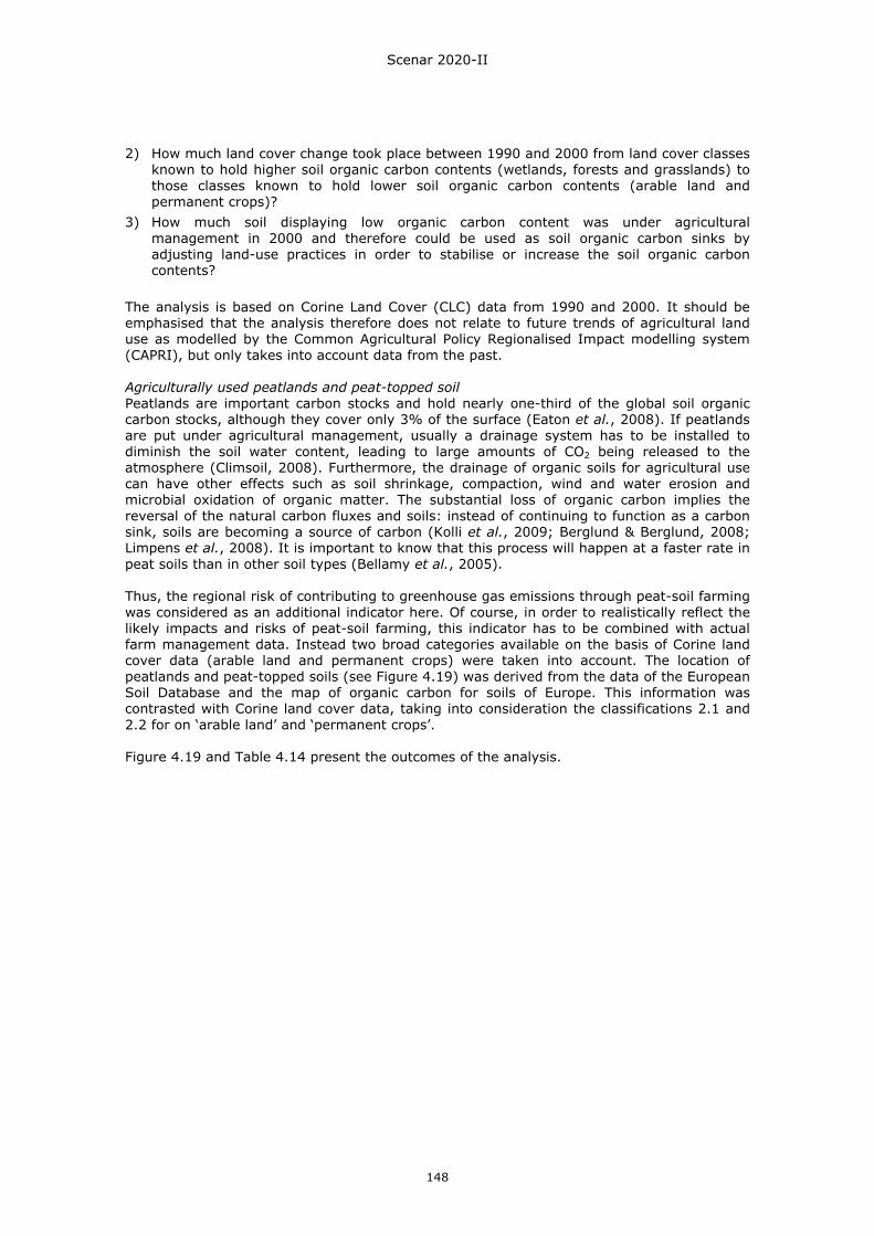
Scenar 2020-II

148

2) How much land cover change took place between 1990 and 2000 from land cover classes known to hold higher soil organic carbon contents (wetlands, forests and grasslands) to those classes known to hold lower soil organic carbon contents (arable land and permanent crops)?

3) How much soil displaying low organic carbon content was under agricultural management in 2000 and therefore could be used as soil organic carbon sinks by adjusting land-use practices in order to stabilise or increase the soil organic carbon contents?

The analysis is based on Corine Land Cover (CLC) data from 1990 and 2000. It should be emphasised that the analysis therefore does not relate to future trends of agricultural land use as modelled by the Common Agricultural Policy Regionalised Impact modelling system (CAPRI), but only takes into account data from the past. Agriculturally used peatlands and peat-topped soil Peatlands are important carbon stocks and hold nearly one-third of the global soil organic carbon stocks, although they cover only 3% of the surface (Eaton et al., 2008). If peatlands are put under agricultural management, usually a drainage system has to be installed to diminish the soil water content, leading to large amounts of CO2 being released to the atmosphere (Climsoil, 2008). Furthermore, the drainage of organic soils for agricultural use can have other effects such as soil shrinkage, compaction, wind and water erosion and microbial oxidation of organic matter. The substantial loss of organic carbon implies the reversal of the natural carbon fluxes and soils: instead of continuing to function as a carbon sink, soils are becoming a source of carbon (Kolli et al., 2009; Berglund & Berglund, 2008; Limpens et al., 2008). It is important to know that this process will happen at a faster rate in peat soils than in other soil types (Bellamy et al., 2005). Thus, the regional risk of contributing to greenhouse gas emissions through peat-soil farming was considered as an additional indicator here. Of course, in order to realistically reflect the likely impacts and risks of peat-soil farming, this indicator has to be combined with actual farm management data. Instead two broad categories available on the basis of Corine land cover data (arable land and permanent crops) were taken into account. The location of peatlands and peat-topped soils (see Figure 4.19) was derived from the data of the European Soil Database and the map of organic carbon for soils of Europe. This information was contrasted with Corine land cover data, taking into consideration the classifications 2.1 and 2.2 for on ‘arable land’ and ‘permanent crops’. Figure 4.19 and Table 4.14 present the outcomes of the analysis.

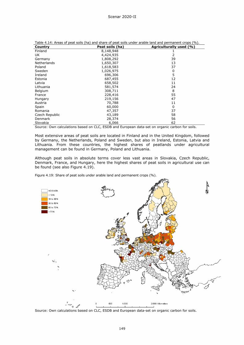
Scenar 2020-II

149

Table 4.14: Areas of peat soils (ha) and share of peat soils under arable land and permanent crops (%). Country Peat soils (ha) Agriculturally used (%) Finland 8,148,948 1 UK 4,424,935 2 Germany 1,808,292 39 Netherlands 1,650,307 13 Poland 1,618,583 37 Sweden 1,026,975 0 Ireland 696,306 5 Estonia 687,455 12 Latvia 658,502 11 Lithuania 581,574 24 Belgium 308,711 8 France 228,416 55 Hungary 219,156 47 Austria 70,788 11 Spain 60,000 0 Romania 47,357 37 Czech Republic 43,189 58 Denmark 28,374 56 Slovakia 6,066 62 Source: Own calculations based on CLC, ESDB and European data-set on organic carbon for soils. Most extensive areas of peat soils are located in Finland and in the United Kingdom, followed by Germany, the Netherlands, Poland and Sweden, but also in Ireland, Estonia, Latvia and Lithuania. From these countries, the highest shares of peatlands under agricultural management can be found in Germany, Poland and Lithuania. Although peat soils in absolute terms cover less vast areas in Slovakia, Czech Republic, Denmark, France, and Hungary, here the highest shares of peat soils in agricultural use can be found (see also Figure 4.19). Figure 4.19: Share of peat soils under arable land and permanent crops (%).

Source: Own calculations based on CLC, ESDB and European data-set on organic carbon for soils.

Scenar 2020-II

150

Land cover change between 1990 and 2000 According to the IPCC (2007), emissions from land-use change amount to approximately 2 petagram carbon per year, which is a significant component in the global carbon cycle (Römkens et al., 1999). As a general rule, soils under forests and grasslands accumulate carbon, whereas soils under arable land usually are a source of carbon, although this also depends on the site conditions and the management practices. The conversion of forests and grasslands to arable land will therefore affect the carbon balance of soils (Levy et al., 2004). In our analysis, we calculated the land cover changes between 1990 and 2000 per FARO region, taking into account changes from wetlands, forests and grassland to agricultural land made up of arable land and permanent crops (see Table 4.15) based on Corine Land Cover data. Table 4.15: Land cover changes from 1990-2000 for the EU-27 as a whole. Conversion from/to 1990-2000

Area (ha) FARO regions affected (n)*

Pasture to arable land 657,916 373 Forest to arable land 17,540 180 Forest to permanent crop 5,936 63 Wetland to arable land 3,225 34 Pasture to permanent crop 2,378 49 Wetland to permanent crop 34 1 Total 687,032 457 * Total number of FARO regions sums up to 857. Source: Own calculations based on Corine Land Cover (CLC) data. The results show that in total nearly 700,000 ha distributed over 457 out of 857 FARO regions are affected by land cover changes, which can be assumed as unfavourable with regard to carbon fluxes between soils and the atmosphere. By far the most land cover changes relate to the conversion of pasture or forests to arable land (see Table 4.15). With regard to conversion of pasture land to arable land, most conversions took place in Ireland (more than 200,000 ha), followed by the Baltic States (almost 150,000 ha). Furthermore, large areas of pastures were changed into arable land in the Netherlands, Hungary, Slovakia, the eastern part of Germany, France and southern Portugal. Forest losses for the benefit of more arable land occur primarily in Spain and south Portugal. Figure 4.20 shows the share of converted land from pasture, forest or wetland to arable land or permanent cultures for all FARO regions.

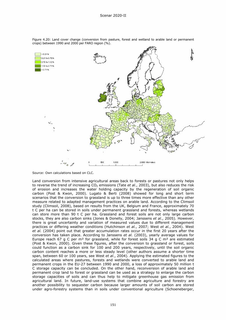
Scenar 2020-II

151

Figure 4.20: Land cover change (conversion from pasture, forest and wetland to arable land or permanent crops) between 1990 and 2000 per FARO region (%).

Source: Own calculations based on CLC. Land conversion from intensive agricultural areas back to forests or pastures not only helps to reverse the trend of increasing CO2 emissions (Tate et al., 2003), but also reduces the risk of erosion and increases the water holding capacity by the regeneration of soil organic carbon (Post & Kwon, 2000). Lugato & Berti (2008) showed for long and short term scenarios that the conversion to grassland is up to three times more effective than any other measure related to adapted management practices on arable land. According to the Climsoil study (Climsoil, 2008), based on results from the UK, Belgium and France, approximately 70 t C per ha can be stored in soils under permanent grassland and forests, whereas wetlands can store more than 90 t C per ha. Grassland and forest soils are not only large carbon stocks, they are also carbon sinks (Jones & Donelly, 2004; Janssens et al., 2005). However, there is great uncertainty and variation of measured values due to different management practices or differing weather conditions (Hutchinson et al., 2007; West et al., 2004). West et al. (2004) point out that greater accumulation rates occur in the first 20 years after the conversion has taken place. According to Janssens et al. (2003), yearly average values for Europe reach 67 g C per m² for grassland, while for forest soils 34 g C m² are estimated (Post & Kwon, 2000). Given these figures, after the conversion to grassland or forest, soils could function as a carbon sink for 100 and 200 years, respectively, until the soil organic carbon content reaches a more or less steady level (other authors assume a shorter time span, between 60 or 100 years, see West et al., 2004). Applying the estimated figures to the calculated areas where pastures, forests and wetlands were converted to arable land and permanent crops in the EU-27 between 1990 and 2000, a loss of approximately 50 million t C storage capacity can be concluded. On the other hand, reconversion of arable land and permanent crop land to forest or grassland can be used as a strategy to enlarge the carbon storage capacities of soils and can thus help to mitigate greenhouse gas emission from agricultural land. In future, land-use systems that combine agriculture and forestry are another possibility to sequester carbon because larger amounts of soil carbon are stored under agro-forestry systems than in soils under conventional agriculture (Schoeneberger,

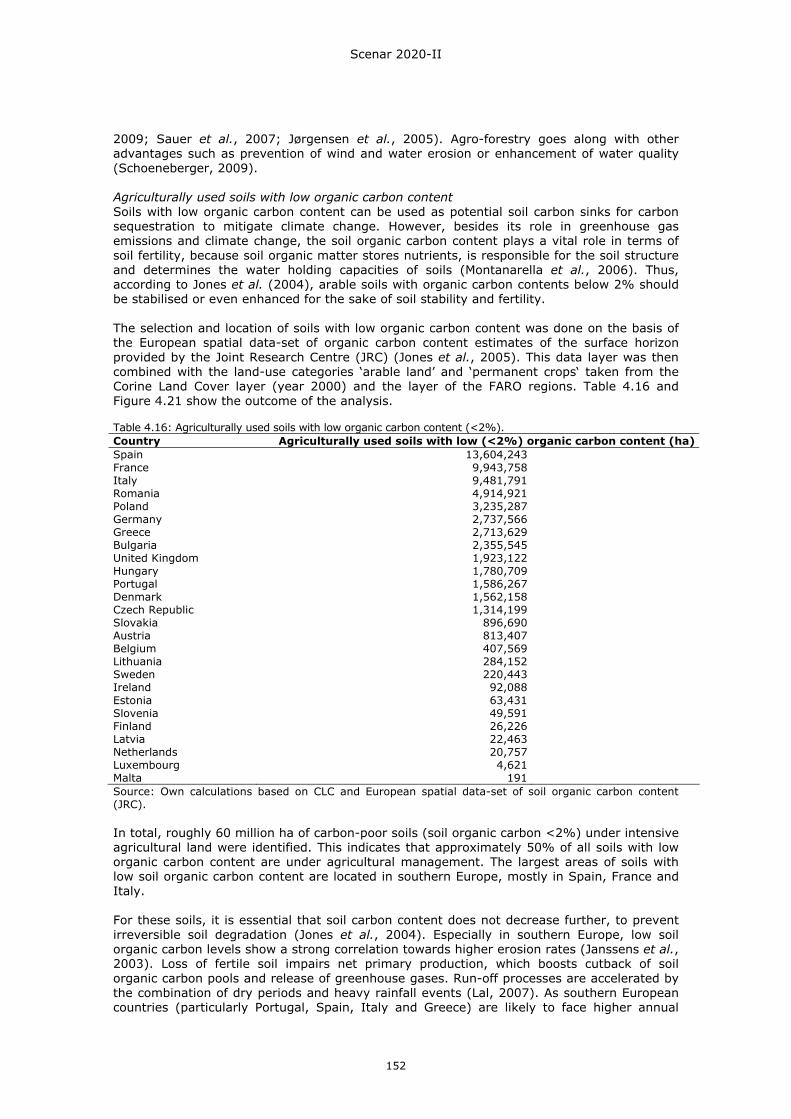
Scenar 2020-II

152

2009; Sauer et al., 2007; Jørgensen et al., 2005). Agro-forestry goes along with other advantages such as prevention of wind and water erosion or enhancement of water quality (Schoeneberger, 2009). Agriculturally used soils with low organic carbon content Soils with low organic carbon content can be used as potential soil carbon sinks for carbon sequestration to mitigate climate change. However, besides its role in greenhouse gas emissions and climate change, the soil organic carbon content plays a vital role in terms of soil fertility, because soil organic matter stores nutrients, is responsible for the soil structure and determines the water holding capacities of soils (Montanarella et al., 2006). Thus, according to Jones et al. (2004), arable soils with organic carbon contents below 2% should be stabilised or even enhanced for the sake of soil stability and fertility. The selection and location of soils with low organic carbon content was done on the basis of the European spatial data-set of organic carbon content estimates of the surface horizon provided by the Joint Research Centre (JRC) (Jones et al., 2005). This data layer was then combined with the land-use categories ‘arable land’ and ‘permanent crops‘ taken from the Corine Land Cover layer (year 2000) and the layer of the FARO regions. Table 4.16 and Figure 4.21 show the outcome of the analysis. Table 4.16: Agriculturally used soils with low organic carbon content (<2%). Country Agriculturally used soils with low (<2%) organic carbon content (ha)Spain 13,604,243France 9,943,758Italy 9,481,791Romania 4,914,921Poland 3,235,287Germany 2,737,566Greece 2,713,629Bulgaria 2,355,545United Kingdom 1,923,122Hungary 1,780,709Portugal 1,586,267Denmark 1,562,158Czech Republic 1,314,199Slovakia 896,690Austria 813,407Belgium 407,569Lithuania 284,152Sweden 220,443Ireland 92,088Estonia 63,431Slovenia 49,591Finland 26,226Latvia 22,463Netherlands 20,757Luxembourg 4,621Malta 191Source: Own calculations based on CLC and European spatial data-set of soil organic carbon content (JRC). In total, roughly 60 million ha of carbon-poor soils (soil organic carbon <2%) under intensive agricultural land were identified. This indicates that approximately 50% of all soils with low organic carbon content are under agricultural management. The largest areas of soils with low soil organic carbon content are located in southern Europe, mostly in Spain, France and Italy. For these soils, it is essential that soil carbon content does not decrease further, to prevent irreversible soil degradation (Jones et al., 2004). Especially in southern Europe, low soil organic carbon levels show a strong correlation towards higher erosion rates (Janssens et al., 2003). Loss of fertile soil impairs net primary production, which boosts cutback of soil organic carbon pools and release of greenhouse gases. Run-off processes are accelerated by the combination of dry periods and heavy rainfall events (Lal, 2007). As southern European countries (particularly Portugal, Spain, Italy and Greece) are likely to face higher annual

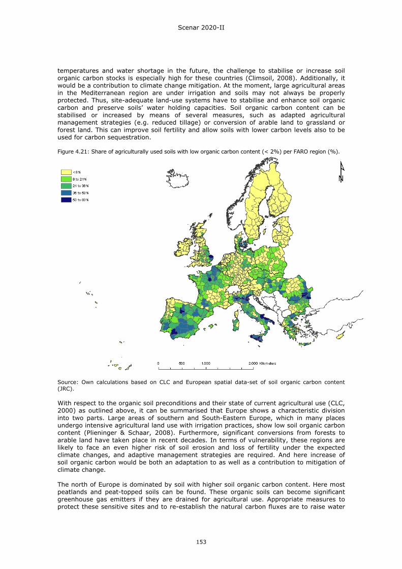
Scenar 2020-II

153

temperatures and water shortage in the future, the challenge to stabilise or increase soil organic carbon stocks is especially high for these countries (Climsoil, 2008). Additionally, it would be a contribution to climate change mitigation. At the moment, large agricultural areas in the Mediterranean region are under irrigation and soils may not always be properly protected. Thus, site-adequate land-use systems have to stabilise and enhance soil organic carbon and preserve soils’ water holding capacities. Soil organic carbon content can be stabilised or increased by means of several measures, such as adapted agricultural management strategies (e.g. reduced tillage) or conversion of arable land to grassland or forest land. This can improve soil fertility and allow soils with lower carbon levels also to be used for carbon sequestration. Figure 4.21: Share of agriculturally used soils with low organic carbon content (< 2%) per FARO region (%).

Source: Own calculations based on CLC and European spatial data-set of soil organic carbon content (JRC). With respect to the organic soil preconditions and their state of current agricultural use (CLC, 2000) as outlined above, it can be summarised that Europe shows a characteristic division into two parts. Large areas of southern and South-Eastern Europe, which in many places undergo intensive agricultural land use with irrigation practices, show low soil organic carbon content (Plieninger & Schaar, 2008). Furthermore, significant conversions from forests to arable land have taken place in recent decades. In terms of vulnerability, these regions are likely to face an even higher risk of soil erosion and loss of fertility under the expected climate changes, and adaptive management strategies are required. And here increase of soil organic carbon would be both an adaptation to as well as a contribution to mitigation of climate change. The north of Europe is dominated by soil with higher soil organic carbon content. Here most peatlands and peat-topped soils can be found. These organic soils can become significant greenhouse gas emitters if they are drained for agricultural use. Appropriate measures to protect these sensitive sites and to re-establish the natural carbon fluxes are to raise water

Scenar 2020-II

154

tables at the cost of initial N2O and CH4 emissions or to establish a perennial and suitable vegetation cover. 4.3.2.6. Biodiversity: Natura 2000 areas

The European Community and its Member States are contracting parties to the UN Convention on Biological Diversity and EU Heads of State and Government agreed to take measures to halt the decline of biodiversity in the EU by 2010 and to restore habitats and natural systems. In this context, Natura 2000 constitutes an ecological network of protected areas in the European Union based on a common political approach to safeguard valuable habitats. The network is designed to designate the most seriously threatened habitats and species across Europe. The underlying legislation for the creation of the Natura 2000 network is made up of two directives: the Habitats Directive (European Commission, 1992) and the Birds Directive (European Commission, 1979). Furthermore, the Natura 2000 areas contribute to the Emerald network of areas of special conservation interest set up under the Bern Convention on the conservation of European wildlife and natural habitats. By December 2008, about 729,430 km² (17% of the total land surface of the EU-27) of the terrestrial area and 129,980 km² of the aquatic area were part of the Natura 2000 network in the EU-27. The number of designated Natura 2000 areas totalled 24,831 sites (European Commission, 2009a). Agricultural land within Natura 2000 areas, arable land as well as grassland, is subject to usage restrictions for reasons of environmental protection. This includes measures concerning extensification, specific management (e.g. cutting or grazing regimes on grassland), and water regimes (Council regulation (EC) No. 1257/1999). The indicator ‘Natura 2000 area’ is therefore not itself a proxy for an environmental vulnerability, but rather one for specific ecological qualities in terms of ‘strengths’; in frequent cases these assets require specific forms of agricultural land use. There is therefore a reinforcing interdependency between the maintenance of these assets and specific forms of management and land use. Here, the indicator is applied to characterise biotic environmental conditions in general, as it is one of the most widely documented indicators for biodiversity throughout Europe and it highlights the areas where conflicts between resource use and resource protection may become likely when facing intensification in agricultural production. However, as the Natura 2000 network is a policy instrument for biodiversity protection, the management plans that Member States have to put in place for each site should ensure positive solutions to such potential conflicts as long as there is sufficient involvement of the key actors and stakeholders in their formulation. The information on the location of Natura 2000 areas per Member State was provided by the European Commission, DG Environment. Based on this information the share of Natura 2000 areas per FARO region was calculated (Figure 4.22) as a measurement of the share of areas important in view of biodiversity protection and habitat preservation per FARO region.

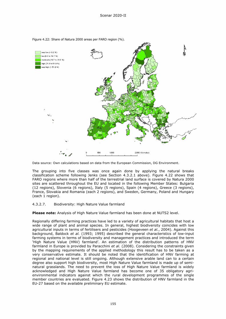
Scenar 2020-II

155

Figure 4.22: Share of Natura 2000 areas per FARO region (%).

Data source: Own calculations based on data from the European Commission, DG Environment. The grouping into five classes was once again done by applying the natural breaks classification scheme following Jenks (see Section 4.3.2.1 above). Figure 4.22 shows that FARO regions where more than half of the terrestrial land surface is covered by Natura 2000 sites are scattered throughout the EU and located in the following Member States: Bulgaria (12 regions), Slovenia (6 regions), Italy (5 regions), Spain (4 regions), Greece (3 regions), France, Slovakia and Romania (each 2 regions), and Sweden, Germany, Poland and Hungary (each 1 region). 4.3.2.7. Biodiversity: High Nature Value farmland

Please note: Analysis of High Nature Value farmland has been done at NUTS2 level. Regionally differing farming practices have led to a variety of agricultural habitats that host a wide range of plant and animal species. In general, highest biodiversity coincides with low agricultural inputs in terms of fertilisers and pesticides (Hoogeveen et al., 2004). Against this background, Baldock et al. (1993; 1995) described the general characteristics of low-input farming systems in terms of biodiversity and management practices and introduced the term ‘High Nature Value (HNV) farmland’. An estimation of the distribution patterns of HNV farmland in Europe is provided by Paracchini et al. (2008). Considering the constraints given by the mapping requirements of the applied methodology this result has to be taken as a very conservative estimate. It should be noted that the identification of HNV farming at regional and national level is still ongoing. Although extensive arable land can to a certain degree also support high biodiversity, most High Nature Value farmland is made up of semi-natural grasslands. The need to prevent the loss of High Nature Value farmland is widely acknowledged and High Nature Value farmland has become one of 35 obligatory agri-environmental indicators against which the rural development programmes of the single member countries are evaluated. Figure 4.23 shows the distribution of HNV farmland in the EU-27 based on the available preliminary EU estimate.

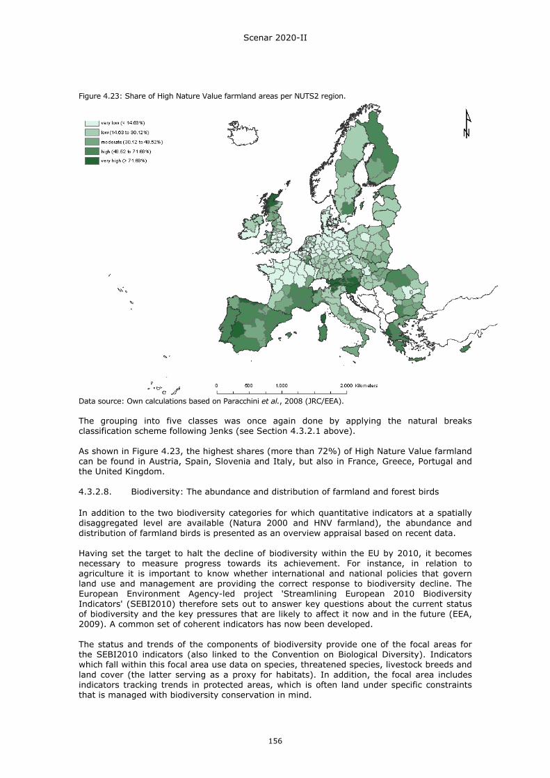
Scenar 2020-II

156

Figure 4.23: Share of High Nature Value farmland areas per NUTS2 region.

Data source: Own calculations based on Paracchini et al., 2008 (JRC/EEA). The grouping into five classes was once again done by applying the natural breaks classification scheme following Jenks (see Section 4.3.2.1 above). As shown in Figure 4.23, the highest shares (more than 72%) of High Nature Value farmland can be found in Austria, Spain, Slovenia and Italy, but also in France, Greece, Portugal and the United Kingdom. 4.3.2.8. Biodiversity: The abundance and distribution of farmland and forest birds

In addition to the two biodiversity categories for which quantitative indicators at a spatially disaggregated level are available (Natura 2000 and HNV farmland), the abundance and distribution of farmland birds is presented as an overview appraisal based on recent data. Having set the target to halt the decline of biodiversity within the EU by 2010, it becomes necessary to measure progress towards its achievement. For instance, in relation to agriculture it is important to know whether international and national policies that govern land use and management are providing the correct response to biodiversity decline. The European Environment Agency-led project 'Streamlining European 2010 Biodiversity Indicators' (SEBI2010) therefore sets out to answer key questions about the current status of biodiversity and the key pressures that are likely to affect it now and in the future (EEA, 2009). A common set of coherent indicators has now been developed. The status and trends of the components of biodiversity provide one of the focal areas for the SEBI2010 indicators (also linked to the Convention on Biological Diversity). Indicators which fall within this focal area use data on species, threatened species, livestock breeds and land cover (the latter serving as a proxy for habitats). In addition, the focal area includes indicators tracking trends in protected areas, which is often land under specific constraints that is managed with biodiversity conservation in mind.

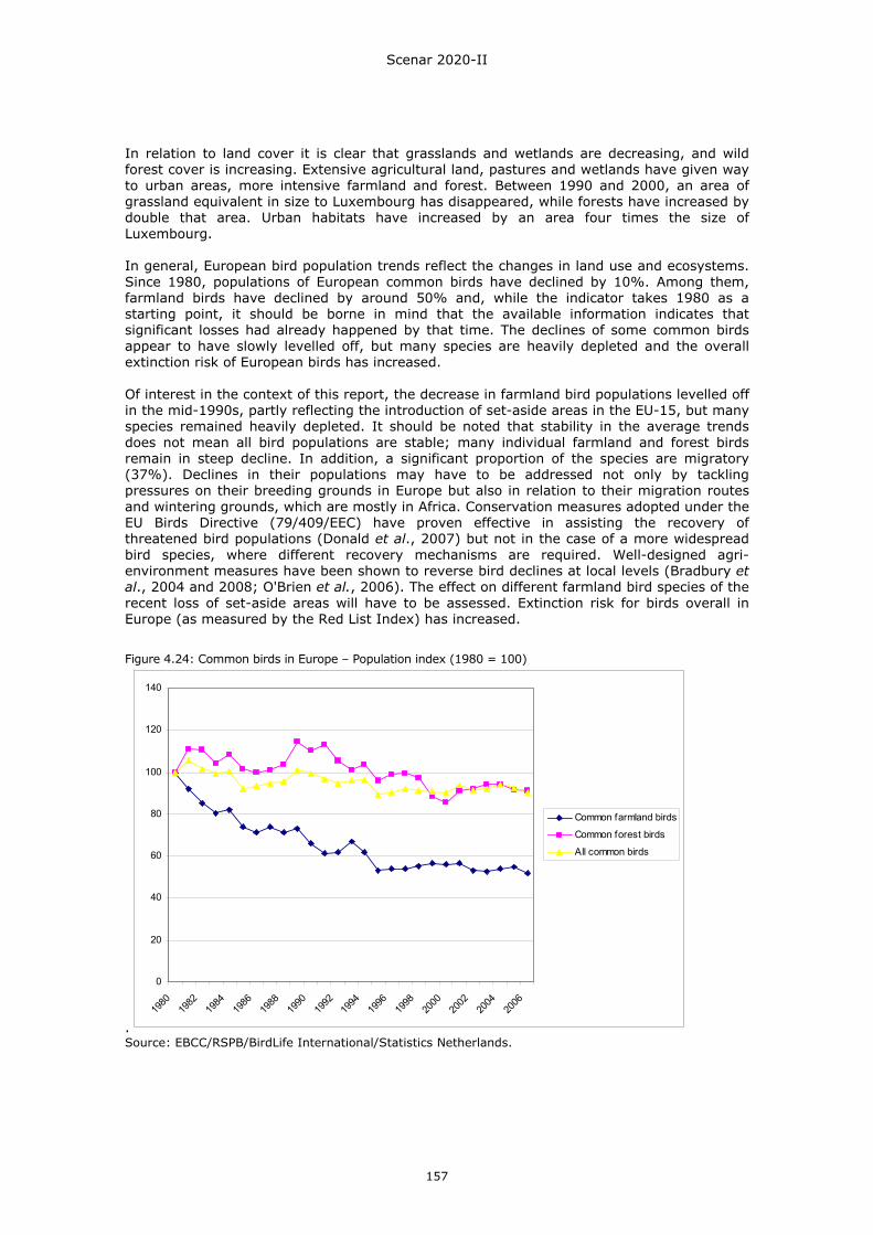
Scenar 2020-II

157

In relation to land cover it is clear that grasslands and wetlands are decreasing, and wild forest cover is increasing. Extensive agricultural land, pastures and wetlands have given way to urban areas, more intensive farmland and forest. Between 1990 and 2000, an area of grassland equivalent in size to Luxembourg has disappeared, while forests have increased by double that area. Urban habitats have increased by an area four times the size of Luxembourg. In general, European bird population trends reflect the changes in land use and ecosystems. Since 1980, populations of European common birds have declined by 10%. Among them, farmland birds have declined by around 50% and, while the indicator takes 1980 as a starting point, it should be borne in mind that the available information indicates that significant losses had already happened by that time. The declines of some common birds appear to have slowly levelled off, but many species are heavily depleted and the overall extinction risk of European birds has increased. Of interest in the context of this report, the decrease in farmland bird populations levelled off in the mid-1990s, partly reflecting the introduction of set-aside areas in the EU-15, but many species remained heavily depleted. It should be noted that stability in the average trends does not mean all bird populations are stable; many individual farmland and forest birds remain in steep decline. In addition, a significant proportion of the species are migratory (37%). Declines in their populations may have to be addressed not only by tackling pressures on their breeding grounds in Europe but also in relation to their migration routes and wintering grounds, which are mostly in Africa. Conservation measures adopted under the EU Birds Directive (79/409/EEC) have proven effective in assisting the recovery of threatened bird populations (Donald et al., 2007) but not in the case of a more widespread bird species, where different recovery mechanisms are required. Well-designed agri-environment measures have been shown to reverse bird declines at local levels (Bradbury et al., 2004 and 2008; O'Brien et al., 2006). The effect on different farmland bird species of the recent loss of set-aside areas will have to be assessed. Extinction risk for birds overall in Europe (as measured by the Red List Index) has increased. Figure 4.24: Common birds in Europe – Population index (1980 = 100)

.

0

20

40

60

80

100

120

140

1980

1982

1984

1986

1988

1990

1992

1994

1996

1998

2000

2002

2004

2006

Common farmland birds

Common forest birds

All common birds

Source: EBCC/RSPB/BirdLife International/Statistics Netherlands.

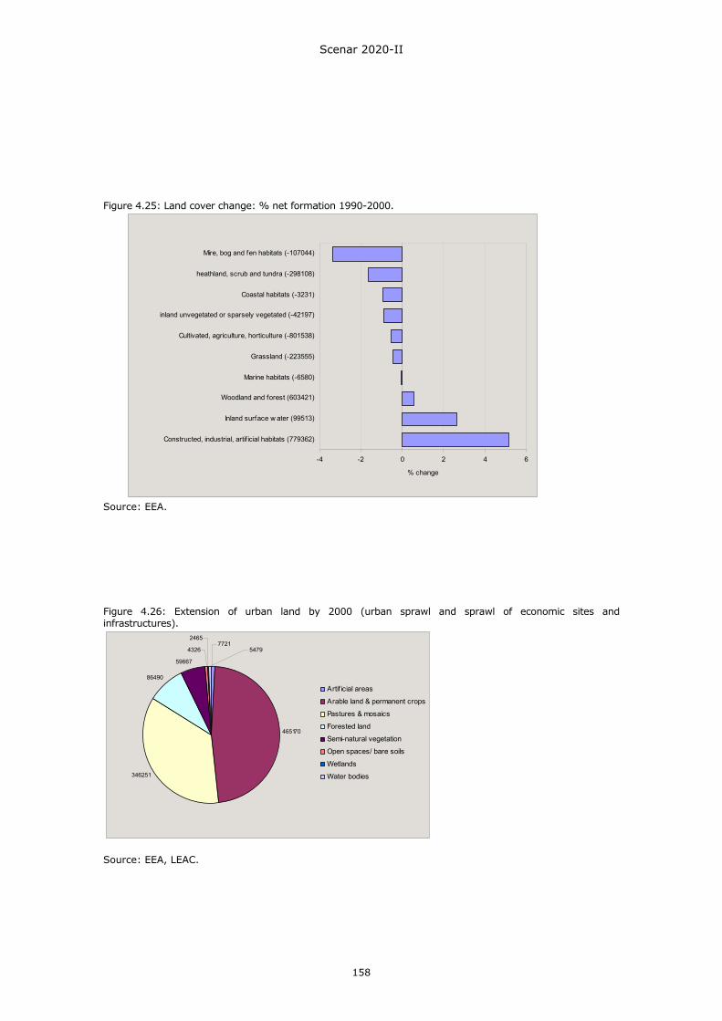
Scenar 2020-II

158

Figure 4.25: Land cover change: % net formation 1990-2000.

-4 -2 0 2 4 6

Constructed, industrial, artif icial habitats (779362)

Inland surface w ater (99513)

Woodland and forest (603421)

Marine habitats (-6580)

Grassland (-223555)

Cultivated, agriculture, horticulture (-801538)

inland unvegetated or sparsely vegetated (-42197)

Coastal habitats (-3231)

heathland, scrub and tundra (-298108)

Mire, bog and fen habitats (-107044)

% change

Source: EEA. Figure 4.26: Extension of urban land by 2000 (urban sprawl and sprawl of economic sites and infrastructures).

465170

346251

86490

59667

4326

24657721

5479

Artif icial areas

Arable land & permanent crops

Pastures & mosaics

Forested land

Semi-natural vegetation

Open spaces/ bare soils

Wetlands

Water bodies

Source: EEA, LEAC.

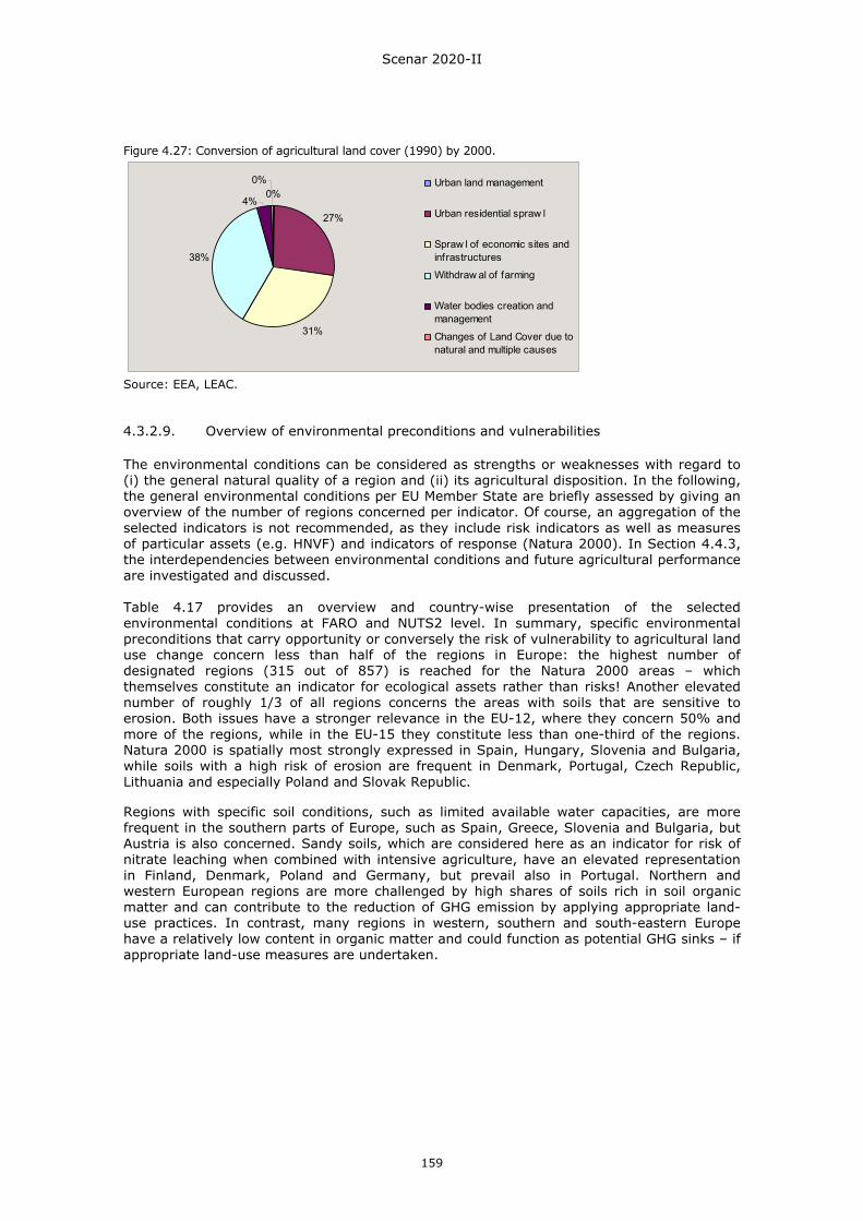
Scenar 2020-II

159

Figure 4.27: Conversion of agricultural land cover (1990) by 2000.

0%

27%

31%

38%

4%

0% Urban land management

Urban residential spraw l

Spraw l of economic sites andinfrastructures

Withdraw al of farming

Water bodies creation andmanagement

Changes of Land Cover due tonatural and multiple causes

Source: EEA, LEAC. 4.3.2.9. Overview of environmental preconditions and vulnerabilities

The environmental conditions can be considered as strengths or weaknesses with regard to (i) the general natural quality of a region and (ii) its agricultural disposition. In the following, the general environmental conditions per EU Member State are briefly assessed by giving an overview of the number of regions concerned per indicator. Of course, an aggregation of the selected indicators is not recommended, as they include risk indicators as well as measures of particular assets (e.g. HNVF) and indicators of response (Natura 2000). In Section 4.4.3, the interdependencies between environmental conditions and future agricultural performance are investigated and discussed. Table 4.17 provides an overview and country-wise presentation of the selected environmental conditions at FARO and NUTS2 level. In summary, specific environmental preconditions that carry opportunity or conversely the risk of vulnerability to agricultural land use change concern less than half of the regions in Europe: the highest number of designated regions (315 out of 857) is reached for the Natura 2000 areas – which themselves constitute an indicator for ecological assets rather than risks! Another elevated number of roughly 1/3 of all regions concerns the areas with soils that are sensitive to erosion. Both issues have a stronger relevance in the EU-12, where they concern 50% and more of the regions, while in the EU-15 they constitute less than one-third of the regions. Natura 2000 is spatially most strongly expressed in Spain, Hungary, Slovenia and Bulgaria, while soils with a high risk of erosion are frequent in Denmark, Portugal, Czech Republic, Lithuania and especially Poland and Slovak Republic. Regions with specific soil conditions, such as limited available water capacities, are more frequent in the southern parts of Europe, such as Spain, Greece, Slovenia and Bulgaria, but Austria is also concerned. Sandy soils, which are considered here as an indicator for risk of nitrate leaching when combined with intensive agriculture, have an elevated representation in Finland, Denmark, Poland and Germany, but prevail also in Portugal. Northern and western European regions are more challenged by high shares of soils rich in soil organic matter and can contribute to the reduction of GHG emission by applying appropriate land-use practices. In contrast, many regions in western, southern and south-eastern Europe have a relatively low content in organic matter and could function as potential GHG sinks – if appropriate land-use measures are undertaken.

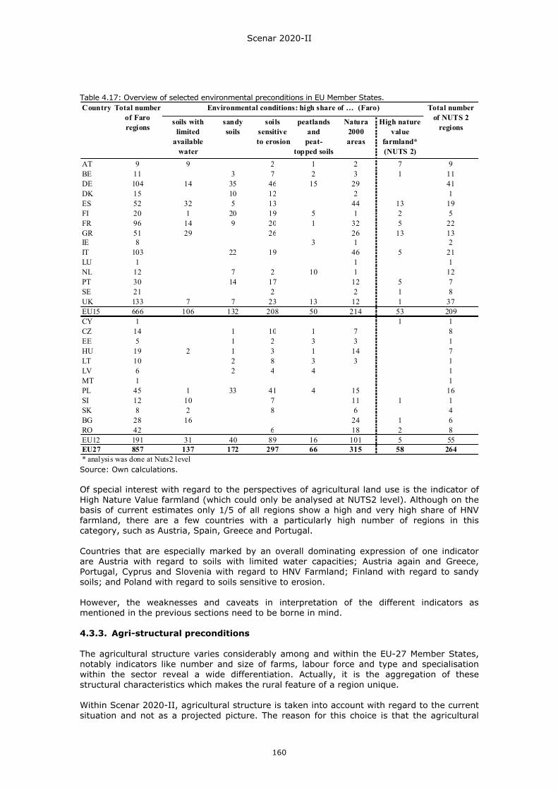
Scenar 2020-II

160

Table 4.17: Overview of selected environmental preconditions in EU Member States.

soils with limited

available water

sandy soils

soils sensitive

to erosion

peatlands and

peat-topped soils

Natura 2000 areas

High nature value

farmland* (NUTS 2)

AT 9 9 2 1 2 7 9BE 11 3 7 2 3 1 11DE 104 14 35 46 15 29 41DK 15 10 12 2 1ES 52 32 5 13 44 13 19FI 20 1 20 19 5 1 2 5FR 96 14 9 20 1 32 5 22GR 51 29 26 26 13 13IE 8 3 1 2IT 103 22 19 46 5 21LU 1 1 1NL 12 7 2 10 1 12PT 30 14 17 12 5 7SE 21 2 2 1 8UK 133 7 7 23 13 12 1 37EU15 666 106 132 208 50 214 53 209CY 1 1 1CZ 14 1 10 1 7 8EE 5 1 2 3 3 1HU 19 2 1 3 1 14 7LT 10 2 8 3 3 1LV 6 2 4 4 1MT 1 1PL 45 1 33 41 4 15 16SI 12 10 7 11 1 1SK 8 2 8 6 4BG 28 16 24 1 6RO 42 6 18 2 8EU12 191 31 40 89 16 101 5 55EU27 857 137 172 297 66 315 58 264* analysis was done at Nuts2 level

Environmental conditions: high share of … (Faro)Country Total number of Faro regions

Total number of NUTS 2

regions

Source: Own calculations. Of special interest with regard to the perspectives of agricultural land use is the indicator of High Nature Value farmland (which could only be analysed at NUTS2 level). Although on the basis of current estimates only 1/5 of all regions show a high and very high share of HNV farmland, there are a few countries with a particularly high number of regions in this category, such as Austria, Spain, Greece and Portugal. Countries that are especially marked by an overall dominating expression of one indicator are Austria with regard to soils with limited water capacities; Austria again and Greece, Portugal, Cyprus and Slovenia with regard to HNV Farmland; Finland with regard to sandy soils; and Poland with regard to soils sensitive to erosion. However, the weaknesses and caveats in interpretation of the different indicators as mentioned in the previous sections need to be borne in mind. 4.3.3. Agri-structural preconditions The agricultural structure varies considerably among and within the EU-27 Member States, notably indicators like number and size of farms, labour force and type and specialisation within the sector reveal a wide differentiation. Actually, it is the aggregation of these structural characteristics which makes the rural feature of a region unique. Within Scenar 2020-II, agricultural structure is taken into account with regard to the current situation and not as a projected picture. The reason for this choice is that the agricultural

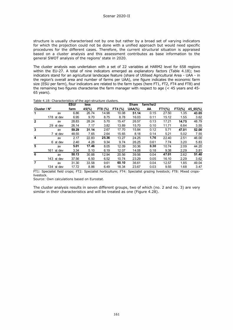
Scenar 2020-II

161

structure is usually characterised not by one but rather by a broad set of varying indicators for which the projection could not be done with a unified approach but would need specific procedures for the different cases. Therefore, the current structural situation is appraised based on a cluster analysis and this assessment contributes as base information to the general SWOT analysis of the regions’ state in 2020. The cluster analysis was undertaken with a set of 22 variables at HARM2 level for 658 regions within the EU-27. A total of nine indicators emerged as explanatory factors (Table 4.18); two indicators stand for an agricultural landscape feature (share of Utilised Agricultural Area - UAA - in the region’s overall area and number of farms per UAA), one figure indicates the economic farm size (ESU per farm), four indicators are related to the farm types (here FT1, FT2, FT4 and FT8) and the remaining two figures characterise the farm manager with respect to age (< 45 years and 45-65 years). Table 4.18: Characteristics of the agri-structure clusters.

Cluster / N° ESU/ farm

less 45(%) FT8 (%) FT4 (%)

Share UAA(%)

farm/haUAA FT1(%) FT2(%) 45_65(%)

1 av 6.86 26.74 14.98 10.08 51.14 0.15 27.50 1.35 43.65178 st dev 6.95 9.70 8.75 8.78 16.03 0.11 15.12 1.55 3.62

2 av 28.83 28.24 5.70 15.47 26.57 0.13 17.21 14.75 48.7929 st dev 26.14 7.17 3.82 13.89 15.70 0.10 11.71 6.84 3.55

3 av 59.29 31.14 2.67 17.70 15.84 0.12 5.71 47.01 52.007 st dev 48.55 7.65 2.64 15.65 8.18 0.14 5.21 5.02 7.55

4 av 2.17 22.83 25.36 13.27 24.25 1.76 22.40 2.51 46.006 st dev 2.40 4.26 9.34 9.74 26.25 0.61 7.74 3.20 5.83

5 av 5.01 17.46 8.05 12.09 30.36 0.30 10.74 2.09 44.20161 st dev 3.34 5.10 6.19 12.07 14.08 0.18 9.38 2.29 3.81

6 av 50.13 30.88 12.94 20.56 39.56 0.04 47.01 2.62 51.40143 st dev 37.56 6.50 6.52 10.74 23.29 0.05 16.10 2.29 3.62

7 av 31.30 33.58 9.61 60.10 36.61 0.04 12.57 1.85 49.04134 st dev 17.72 8.86 6.49 18.34 23.67 0.03 9.55 1.68 3.47

FT1: Specialist field crops; FT2: Specialist horticulture; FT4: Specialist grazing livestock; FT8: Mixed crops-livestock. Source: Own calculations based on Eurostat. The cluster analysis results in seven different groups, two of which (no. 2 and no. 3) are very similar in their characteristics and will be treated as one (Figure 4.28).

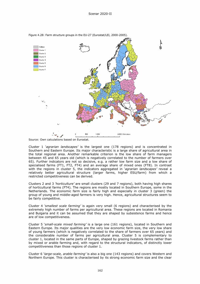
Scenar 2020-II

162

Figure 4.28: Farm structure groups in the EU-27 (Eurostat/LEI, 2000-2005).

Source: Own calculations based on Eurostat. Cluster 1 ‘agrarian landscapes’ is the largest one (178 regions) and is concentrated in Southern and Eastern Europe. Its major characteristic is a large share of agricultural area in the total regional area. Another remarkable criterion is the low share of farm managers between 45 and 65 years old (which is negatively correlated to the number of farmers over 65). Further indicators are not so decisive, e.g. a rather low farm size and a low share of specialised farms (FT1, FT2, FT4) and an average share of mixed ones (FT8). In contrast with the regions in cluster 5, the indicators aggregated in ‘agrarian landscapes’ reveal a relatively better agricultural structure (larger farms, higher ESU/farm) from which a restricted competitiveness can be derived. Clusters 2 and 3 ‘horticulture’ are small clusters (29 and 7 regions), both having high shares of horticultural farms (FT4). The regions are mostly located in Southern Europe, some in the Netherlands. The economic farm size is fairly high and especially in cluster 3 (green) the group of young and middle-aged farmers is very high. Hence, agricultural structures seem to be fairly competitive. Cluster 4 ‘smallest scale farming’ is again very small (6 regions) and characterised by the extremely high number of farms per agricultural area. These regions are located in Romania and Bulgaria and it can be assumed that they are shaped by subsistence farms and hence are of low competitiveness. Cluster 5 ‘small-scale mixed farming’ is a large one (161 regions), located in Southern and Eastern Europe. Its major qualities are the very low economic farm size, the very low share of young farmers (which is negatively correlated to the share of farmers over 65 years) and the considerable number of farms per agricultural area. Cluster 5 is complementary to cluster 1, located in the same parts of Europe, shaped by grazing livestock farms rather than by mixed or arable farming and, with regard to the structural indicators, of distinctly lower competitiveness than those regions of cluster 1. Cluster 6 ‘large-scale, arable farming’ is also a big one (143 regions) and covers Western and Northern Europe. This cluster is characterised by its strong economic farm size and the clear

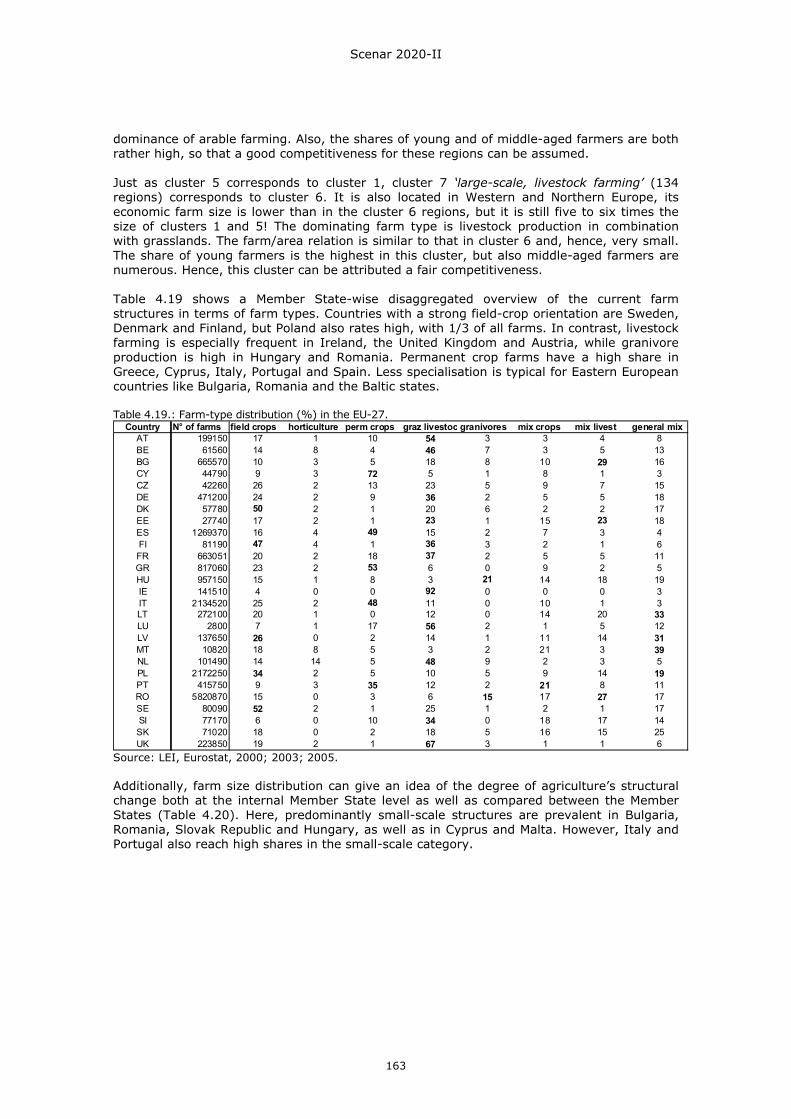
Scenar 2020-II

163

dominance of arable farming. Also, the shares of young and of middle-aged farmers are both rather high, so that a good competitiveness for these regions can be assumed. Just as cluster 5 corresponds to cluster 1, cluster 7 ‘large-scale, livestock farming’ (134 regions) corresponds to cluster 6. It is also located in Western and Northern Europe, its economic farm size is lower than in the cluster 6 regions, but it is still five to six times the size of clusters 1 and 5! The dominating farm type is livestock production in combination with grasslands. The farm/area relation is similar to that in cluster 6 and, hence, very small. The share of young farmers is the highest in this cluster, but also middle-aged farmers are numerous. Hence, this cluster can be attributed a fair competitiveness. Table 4.19 shows a Member State-wise disaggregated overview of the current farm structures in terms of farm types. Countries with a strong field-crop orientation are Sweden, Denmark and Finland, but Poland also rates high, with 1/3 of all farms. In contrast, livestock farming is especially frequent in Ireland, the United Kingdom and Austria, while granivore production is high in Hungary and Romania. Permanent crop farms have a high share in Greece, Cyprus, Italy, Portugal and Spain. Less specialisation is typical for Eastern European countries like Bulgaria, Romania and the Baltic states. Table 4.19.: Farm-type distribution (%) in the EU-27.

Country N° of farms field crops horticulture perm crops graz livestoc granivores mix crops mix livest general mixAT 199150 17 1 10 54 3 3 4 8BE 61560 14 8 4 46 7 3 5 13BG 665570 10 3 5 18 8 10 29 16CY 44790 9 3 72 5 1 8 1 3CZ 42260 26 2 13 23 5 9 7 15DE 471200 24 2 9 36 2 5 5 18DK 57780 50 2 1 20 6 2 2 17EE 27740 17 2 1 23 1 15 23 18ES 1269370 16 4 49 15 2 7 3 4FI 81190 47 4 1 36 3 2 1 6FR 663051 20 2 18 37 2 5 5 11GR 817060 23 2 53 6 0 9 2 5HU 957150 15 1 8 3 21 14 18 19IE 141510 4 0 0 92 0 0 0 3IT 2134520 25 2 48 11 0 10 1 3LT 272100 20 1 0 12 0 14 20 33LU 2800 7 1 17 56 2 1 5 12LV 137650 26 0 2 14 1 11 14 31MT 10820 18 8 5 3 2 21 3 39NL 101490 14 14 5 48 9 2 3 5PL 2172250 34 2 5 10 5 9 14 19PT 415750 9 3 35 12 2 21 8 11RO 5820870 15 0 3 6 15 17 27 17SE 80090 52 2 1 25 1 2 1 17SI 77170 6 0 10 34 0 18 17 14SK 71020 18 0 2 18 5 16 15 25UK 223850 19 2 1 67 3 1 1 6

Source: LEI, Eurostat, 2000; 2003; 2005. Additionally, farm size distribution can give an idea of the degree of agriculture’s structural change both at the internal Member State level as well as compared between the Member States (Table 4.20). Here, predominantly small-scale structures are prevalent in Bulgaria, Romania, Slovak Republic and Hungary, as well as in Cyprus and Malta. However, Italy and Portugal also reach high shares in the small-scale category.

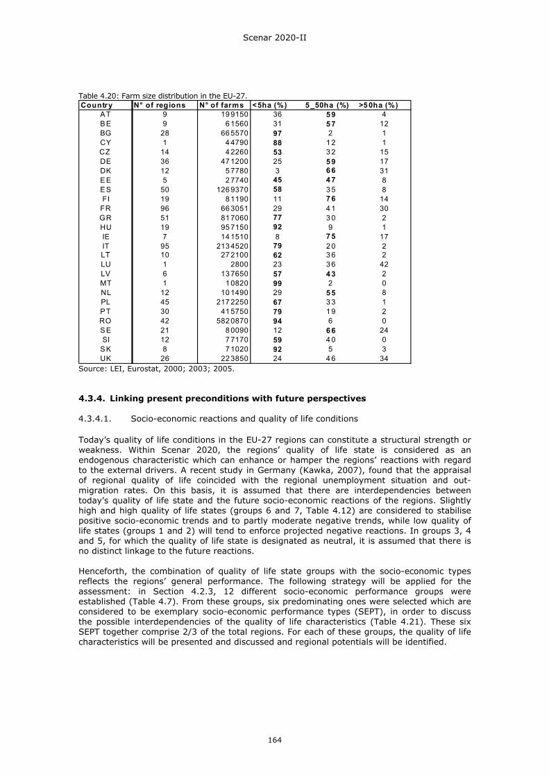
Scenar 2020-II

164

Table 4.20: Farm size distribution in the EU-27. Country N° of regions N° of farms <5ha (%) 5 _50ha (%) >5 0ha (%)

AT 9 19 9150 36 5 9 4BE 9 6 1560 31 5 7 12BG 28 66 5570 97 2 1CY 1 4 4790 88 1 2 1CZ 14 4 2260 53 3 2 15DE 36 47 1200 25 5 9 17DK 12 5 7780 3 6 6 31EE 5 2 7740 45 4 7 8ES 50 126 9370 58 3 5 8FI 19 8 1190 11 7 6 14

FR 96 66 3051 29 4 1 30GR 51 81 7060 77 3 0 2HU 19 95 7150 92 9 1IE 7 14 1510 8 7 5 17IT 95 213 4520 79 2 0 2LT 10 27 2100 62 3 6 2LU 1 2800 23 3 6 42LV 6 13 7650 57 4 3 2MT 1 1 0820 99 2 0NL 12 10 1490 29 5 5 8PL 45 217 2250 67 3 3 1PT 30 41 5750 79 1 9 2RO 42 582 0870 94 6 0SE 21 8 0090 12 6 6 24SI 12 7 7170 59 4 0 0

SK 8 7 1020 92 5 3UK 26 22 3850 24 4 6 34

Source: LEI, Eurostat, 2000; 2003; 2005. 4.3.4. Linking present preconditions with future perspectives 4.3.4.1. Socio-economic reactions and quality of life conditions

Today’s quality of life conditions in the EU-27 regions can constitute a structural strength or weakness. Within Scenar 2020, the regions’ quality of life state is considered as an endogenous characteristic which can enhance or hamper the regions’ reactions with regard to the external drivers. A recent study in Germany (Kawka, 2007), found that the appraisal of regional quality of life coincided with the regional unemployment situation and out-migration rates. On this basis, it is assumed that there are interdependencies between today’s quality of life state and the future socio-economic reactions of the regions. Slightly high and high quality of life states (groups 6 and 7, Table 4.12) are considered to stabilise positive socio-economic trends and to partly moderate negative trends, while low quality of life states (groups 1 and 2) will tend to enforce projected negative reactions. In groups 3, 4 and 5, for which the quality of life state is designated as neutral, it is assumed that there is no distinct linkage to the future reactions. Henceforth, the combination of quality of life state groups with the socio-economic types reflects the regions’ general performance. The following strategy will be applied for the assessment: in Section 4.2.3, 12 different socio-economic performance groups were established (Table 4.7). From these groups, six predominating ones were selected which are considered to be exemplary socio-economic performance types (SEPT), in order to discuss the possible interdependencies of the quality of life characteristics (Table 4.21). These six SEPT together comprise 2/3 of the total regions. For each of these groups, the quality of life characteristics will be presented and discussed and regional potentials will be identified.

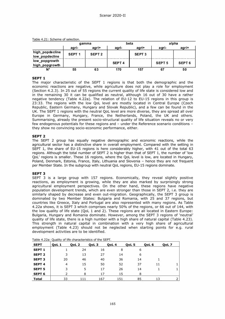
Scenar 2020-II

165

Table 4.21: Scheme of selection.

agri- agri+ agri- agri+ agri- agri+high_popdeclinelow_popdeclinelow_popgrowthhigh_popgrowth

N° 55 63 170 157 67 50

gamma beta alpha

SEPT 6

SEPT 3SEPT 1 SEPT 2

SEPT 4 SEPT 5

SEPT 1 The major characteristic of the SEPT 1 regions is that both the demographic and the economic reactions are negative, while agriculture does not play a role for employment (Section 4.2.3). In 25 out of 55 regions the current quality of life state is considered low and in the remaining 30 it can be qualified as neutral, although 16 out of 30 have a rather negative tendency (Table 4.22a). The relation of EU-12 to EU-15 regions in this group is 23:33. The regions with the low QoL level are mostly located in Central Europe (Czech Republic, Eastern Germany, Hungary and Slovak Republic), and a few can be found in the UK. The SEPT 1 regions with the neutral QoL level are more diverse, they are spread all over Europe in Germany, Hungary, France, the Netherlands, Poland, the UK and others. Summarising, already the present socio-structural quality of life situation reveals no or very few endogenous potentials for these regions and – under the Reference scenario conditions – they show no convincing socio-economic performance, either. SEPT 2 The SEPT 2 group has equally negative demographic and economic reactions, while the agricultural sector has a distinctive share in overall employment. Compared with the setting in SEPT 1, the share of EU-15 regions is here considerably higher, with 41 out of the total 63 regions. Although the total number of SEPT 2 is higher than that of SEPT 1, the number of ‘low QoL’ regions is smaller. These 16 regions, where the QoL level is low, are located in Hungary, Poland, Denmark, Estonia, France, Italy, Lithuania and Slovenia – hence they are not frequent per Member State. In the subgroup with neutral QoL regions, EU-15 regions dominate. SEPT 3 SEPT 3 is a large group with 157 regions. Economically, they reveal slightly positive reactions, as employment is growing, while they are also marked by surprisingly strong agricultural employment perspectives. On the other hand, these regions have negative population development trends, which are even stronger than those in SEPT 2, i.e. they are similarly shaped by decrease and even out-migration. Geographically, the SEPT 3 group is dominated by two Member States: Bulgaria and Romania, with 25 and 37 regions, but countries like Greece, Italy and Portugal are also represented with many regions. As Table 4.22a shows, it is SEPT 3 which comprises nearly 50% of the regions, or 66 out of 144, with the low quality of life state (QoL 1 and 2). These regions are all located in Eastern Europe: Bulgaria, Hungary and Romania dominate. However, among the SEPT 3 regions of ‘neutral’ quality of life state, there is a high number with a high share of natural capital (Table 4.23). This strength in natural capital in combination with a very high share of agricultural employment (Table 4.23) should not be neglected when starting points for e.g. rural development activities are to be identified. Table 4.22a: Quality of life characteristics of the SEPT.

SEPT QoL 1 QoL 2 QoL 3 QoL 4 QoL 5 QoL 6 QoL 7

SEPT 1 1 24 16 8 6 SEPT 2 3 13 27 14 6 SEPT 3 20 46 40 36 14 1 SEPT 4 4 15 50 52 37 11 1 SEPT 5 3 5 17 26 14 1 1 SEPT 6 2 8 17 15 8

Total 33 111 167 151 85 13 2

Scenar 2020-II

166

Table 4.22b: Regions according to OECD types per SEPT.

SEPT MR IR MU total

SEPT 1 13 26 16 55SEPT 2 50 11 2 63SEPT 3 114 42 1 157SEPT 4 25 62 83 170SEPT 5 12 30 25 67SEPT 6 22 27 1 50

Total 236 198 128 562 SEPT 4 The SEPT 4 group is also a large group that consists of 170 regions. This group has a moderate positive perspective in demographic and economic dynamics. Its share of agricultural employment in 2020 is the lowest of all groups (equal to SEPT 1; Table 4.23). The relation of low QoL groups to the neutral and high ones is 19:139:12. Hence, the structural quality of life preconditions are neutral to favourable and seem to enforce the positive socio-economic reactions that these regions show. In this group, 32 out of 104 German regions, 22 out of 96 French regions, 8 out of 20 Swedish regions, and 55 out of 133 UK regions can be found. Hence, it has a strong dominance of EU-15 regions, and comprises the largest share of most urban regions. Thus, the current characteristics of built and social capital are the highest of all SEPT, while the natural capital is the second lowest. Obviously, these regions are weak in favourable landscape amenities and natural ecosystems. SEPT 5 The SEPT 5 group comprises 67 regions with a strong socio-economic perspective that is not contrasted by a strong primary sector employment. The dominating quality of life state is neutral. From the EU-12, only 6 Polish regions, Cyprus and Malta are represented, while the remaining 59 EU-15 regions are mainly located in (Western) Germany, France, Italy, Spain and the UK. The quality of life preconditions in the SEPT 5 group are fairly similar to those of SEPT 4, except that the natural capital index has a higher average share. SEPT 6 Although SEPT 6 has nearly similar socio-economic conditions to SEPT 5, along with an above average agricultural employment perspective, the distribution of the structural conditions that make a quality of life are quite different: here, no regions with a high QoL state are represented and there is a relatively high share of regions with a low QoL state (10 out of 50), located in Germany (3), Italy (1), Spain (5) and Portugal (1). Only one region of EU-12 Member States can be found (Latvia). Hence, these SEPT 6 regions are characterised by a current low to neutral quality of life state and positive future perspectives and a strong agricultural sector (in terms of employment, at least). This can be cautiously interpreted as an indication that here is no correlation between socio-economic development perspectives as derived from the models and time series and today’s quality of life structures as captured by the selection of indicators. Table 4.23: Averages of key indicators per SEPT.

GDPperCapita GVA in services GBLI_weighted emplgrowth 04_20 shAgriEmp20 popgr04_20SEPT 1 17533.25 64.76 48.38 -0.42 1.47 -0.60SEPT 2 15479.47 64.44 55.94 -0.41 8.41 -0.37SEPT 3 11314.10 57.56 60.99 0.21 15.87 -0.62SEPT 4 25699.25 69.18 50.78 0.24 1.47 0.36SEPT 5 24117.27 68.73 54.37 0.94 1.52 0.63SEPT 6 20721.23 64.02 64.11 0.90 8.96 0.74total average 19144.10 64.78 55.76 0.24 6.28 0.02 Summarising this cross-sectional analysis, it has first to be noted that there is no straight conceptual assumption about a linkage between current quality of life conditions and future socio-economic reactions of the regions. However, the findings are interpreted in terms of mutually enforcing or hindering strengths and weaknesses. In this realm, it becomes obvious that the regions with a weak socio-economic reaction in 2020 (SEPT 1 and SEPT 2) are also

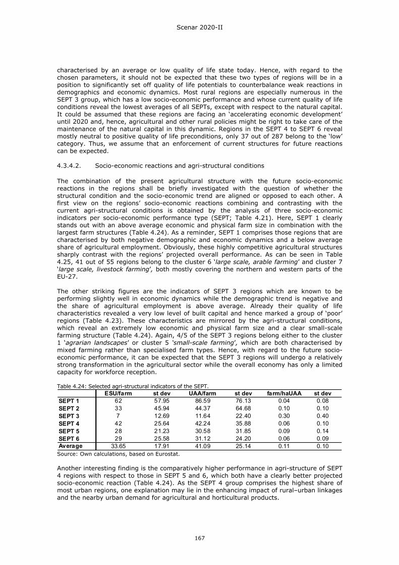
Scenar 2020-II

167

characterised by an average or low quality of life state today. Hence, with regard to the chosen parameters, it should not be expected that these two types of regions will be in a position to significantly set off quality of life potentials to counterbalance weak reactions in demographics and economic dynamics. Most rural regions are especially numerous in the SEPT 3 group, which has a low socio-economic performance and whose current quality of life conditions reveal the lowest averages of all SEPTs, except with respect to the natural capital. It could be assumed that these regions are facing an ‘accelerating economic development’ until 2020 and, hence, agricultural and other rural policies might be right to take care of the maintenance of the natural capital in this dynamic. Regions in the SEPT 4 to SEPT 6 reveal mostly neutral to positive quality of life preconditions, only 37 out of 287 belong to the ‘low’ category. Thus, we assume that an enforcement of current structures for future reactions can be expected. 4.3.4.2. Socio-economic reactions and agri-structural conditions

The combination of the present agricultural structure with the future socio-economic reactions in the regions shall be briefly investigated with the question of whether the structural condition and the socio-economic trend are aligned or opposed to each other. A first view on the regions’ socio-economic reactions combining and contrasting with the current agri-structural conditions is obtained by the analysis of three socio-economic indicators per socio-economic performance type (SEPT; Table 4.21). Here, SEPT 1 clearly stands out with an above average economic and physical farm size in combination with the largest farm structures (Table 4.24). As a reminder, SEPT 1 comprises those regions that are characterised by both negative demographic and economic dynamics and a below average share of agricultural employment. Obviously, these highly competitive agricultural structures sharply contrast with the regions’ projected overall performance. As can be seen in Table 4.25, 41 out of 55 regions belong to the cluster 6 ‘large scale, arable farming’ and cluster 7 ‘large scale, livestock farming’, both mostly covering the northern and western parts of the EU-27. The other striking figures are the indicators of SEPT 3 regions which are known to be performing slightly well in economic dynamics while the demographic trend is negative and the share of agricultural employment is above average. Already their quality of life characteristics revealed a very low level of built capital and hence marked a group of ‘poor’ regions (Table 4.23). These characteristics are mirrored by the agri-structural conditions, which reveal an extremely low economic and physical farm size and a clear small-scale farming structure (Table 4.24). Again, 4/5 of the SEPT 3 regions belong either to the cluster 1 ‘agrarian landscapes’ or cluster 5 ‘small-scale farming’, which are both characterised by mixed farming rather than specialised farm types. Hence, with regard to the future socio-economic performance, it can be expected that the SEPT 3 regions will undergo a relatively strong transformation in the agricultural sector while the overall economy has only a limited capacity for workforce reception. Table 4.24: Selected agri-structural indicators of the SEPT.

ESU/farm st dev UAA/farm st dev farm/haUAA st devSEPT 1 62 57.95 86.59 76.13 0.04 0.08SEPT 2 33 45.94 44.37 64.68 0.10 0.10SEPT 3 7 12.69 11.64 22.40 0.30 0.40SEPT 4 42 25.64 42.24 35.88 0.06 0.10SEPT 5 28 21.23 30.58 31.85 0.09 0.14SEPT 6 29 25.58 31.12 24.20 0.06 0.09Average 33.65 17.91 41.09 25.14 0.11 0.10 Source: Own calculations, based on Eurostat. Another interesting finding is the comparatively higher performance in agri-structure of SEPT 4 regions with respect to those in SEPT 5 and 6, which both have a clearly better projected socio-economic reaction (Table 4.24). As the SEPT 4 group comprises the highest share of most urban regions, one explanation may lie in the enhancing impact of rural–urban linkages and the nearby urban demand for agricultural and horticultural products.

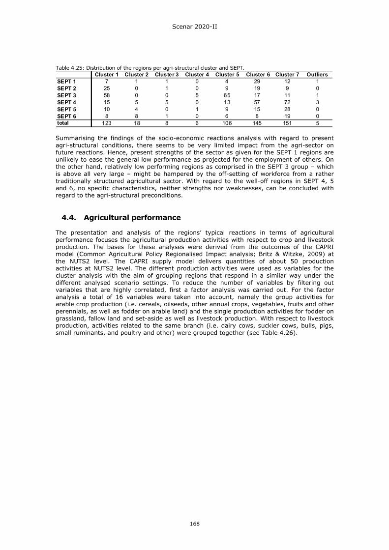
Scenar 2020-II

168

Table 4.25: Distribution of the regions per agri-structural cluster and SEPT. Cluster 1 Cluster 2 Cluster 3 Cluster 4 Cluster 5 Cluster 6 Cluster 7 Outliers

SEPT 1 7 1 1 0 4 29 12 1SEPT 2 25 0 1 0 9 19 9 0SEPT 3 58 0 0 5 65 17 11 1SEPT 4 15 5 5 0 13 57 72 3SEPT 5 10 4 0 1 9 15 28 0SEPT 6 8 8 1 0 6 8 19 0total 123 18 8 6 106 145 151 5 Summarising the findings of the socio-economic reactions analysis with regard to present agri-structural conditions, there seems to be very limited impact from the agri-sector on future reactions. Hence, present strengths of the sector as given for the SEPT 1 regions are unlikely to ease the general low performance as projected for the employment of others. On the other hand, relatively low performing regions as comprised in the SEPT 3 group – which is above all very large – might be hampered by the off-setting of workforce from a rather traditionally structured agricultural sector. With regard to the well-off regions in SEPT 4, 5 and 6, no specific characteristics, neither strengths nor weaknesses, can be concluded with regard to the agri-structural preconditions.

4.4. Agricultural performance The presentation and analysis of the regions’ typical reactions in terms of agricultural performance focuses the agricultural production activities with respect to crop and livestock production. The bases for these analyses were derived from the outcomes of the CAPRI model (Common Agricultural Policy Regionalised Impact analysis; Britz & Witzke, 2009) at the NUTS2 level. The CAPRI supply model delivers quantities of about 50 production activities at NUTS2 level. The different production activities were used as variables for the cluster analysis with the aim of grouping regions that respond in a similar way under the different analysed scenario settings. To reduce the number of variables by filtering out variables that are highly correlated, first a factor analysis was carried out. For the factor analysis a total of 16 variables were taken into account, namely the group activities for arable crop production (i.e. cereals, oilseeds, other annual crops, vegetables, fruits and other perennials, as well as fodder on arable land) and the single production activities for fodder on grassland, fallow land and set-aside as well as livestock production. With respect to livestock production, activities related to the same branch (i.e. dairy cows, suckler cows, bulls, pigs, small ruminants, and poultry and other) were grouped together (see Table 4.26).

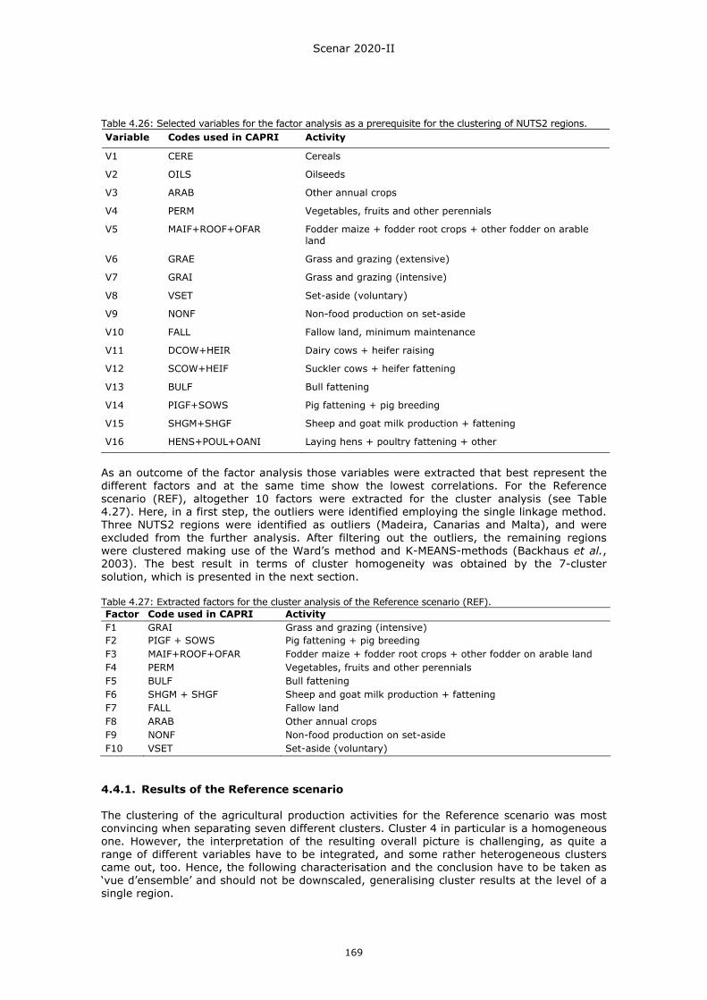
Scenar 2020-II

169

Table 4.26: Selected variables for the factor analysis as a prerequisite for the clustering of NUTS2 regions. Variable Codes used in CAPRI Activity

V1 CERE Cereals

V2 OILS Oilseeds

V3 ARAB Other annual crops

V4 PERM Vegetables, fruits and other perennials

V5 MAIF+ROOF+OFAR Fodder maize + fodder root crops + other fodder on arable land

V6 GRAE Grass and grazing (extensive)

V7 GRAI Grass and grazing (intensive)

V8 VSET Set-aside (voluntary)

V9 NONF Non-food production on set-aside

V10 FALL Fallow land, minimum maintenance

V11 DCOW+HEIR Dairy cows + heifer raising

V12 SCOW+HEIF Suckler cows + heifer fattening

V13 BULF Bull fattening

V14 PIGF+SOWS Pig fattening + pig breeding

V15 SHGM+SHGF Sheep and goat milk production + fattening

V16 HENS+POUL+OANI Laying hens + poultry fattening + other

As an outcome of the factor analysis those variables were extracted that best represent the different factors and at the same time show the lowest correlations. For the Reference scenario (REF), altogether 10 factors were extracted for the cluster analysis (see Table 4.27). Here, in a first step, the outliers were identified employing the single linkage method. Three NUTS2 regions were identified as outliers (Madeira, Canarias and Malta), and were excluded from the further analysis. After filtering out the outliers, the remaining regions were clustered making use of the Ward’s method and K-MEANS-methods (Backhaus et al., 2003). The best result in terms of cluster homogeneity was obtained by the 7-cluster solution, which is presented in the next section. Table 4.27: Extracted factors for the cluster analysis of the Reference scenario (REF). Factor Code used in CAPRI Activity F1 GRAI Grass and grazing (intensive) F2 PIGF + SOWS Pig fattening + pig breeding F3 MAIF+ROOF+OFAR Fodder maize + fodder root crops + other fodder on arable land F4 PERM Vegetables, fruits and other perennials F5 BULF Bull fattening F6 SHGM + SHGF Sheep and goat milk production + fattening F7 FALL Fallow land F8 ARAB Other annual crops F9 NONF Non-food production on set-aside F10 VSET Set-aside (voluntary)

4.4.1. Results of the Reference scenario The clustering of the agricultural production activities for the Reference scenario was most convincing when separating seven different clusters. Cluster 4 in particular is a homogeneous one. However, the interpretation of the resulting overall picture is challenging, as quite a range of different variables have to be integrated, and some rather heterogeneous clusters came out, too. Hence, the following characterisation and the conclusion have to be taken as ‘vue d’ensemble’ and should not be downscaled, generalising cluster results at the level of a single region.

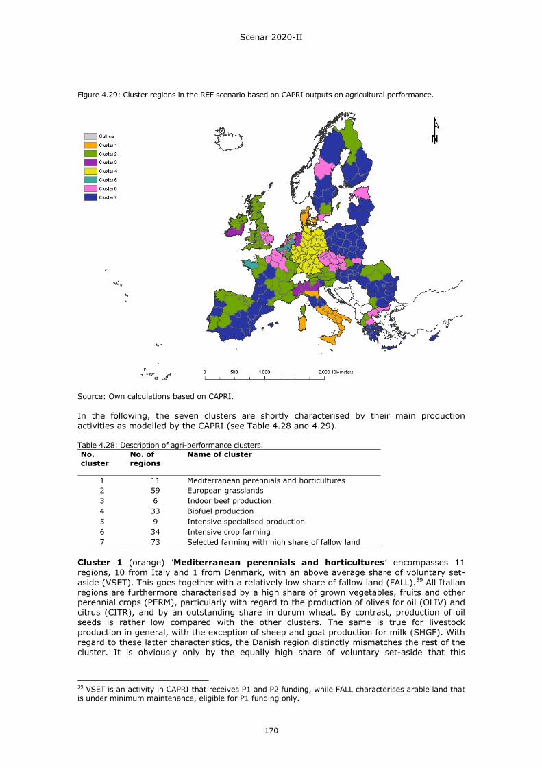
Scenar 2020-II

170

Figure 4.29: Cluster regions in the REF scenario based on CAPRI outputs on agricultural performance.

Source: Own calculations based on CAPRI. In the following, the seven clusters are shortly characterised by their main production activities as modelled by the CAPRI (see Table 4.28 and 4.29). Table 4.28: Description of agri-performance clusters. No. cluster

No. of regions

Name of cluster

1 11 Mediterranean perennials and horticultures 2 59 European grasslands 3 6 Indoor beef production 4 33 Biofuel production 5 9 Intensive specialised production 6 34 Intensive crop farming 7 73 Selected farming with high share of fallow land

Cluster 1 (orange) ’Mediterranean perennials and horticultures’ encompasses 11 regions, 10 from Italy and 1 from Denmark, with an above average share of voluntary set-aside (VSET). This goes together with a relatively low share of fallow land (FALL).39 All Italian regions are furthermore characterised by a high share of grown vegetables, fruits and other perennial crops (PERM), particularly with regard to the production of olives for oil (OLIV) and citrus (CITR), and by an outstanding share in durum wheat. By contrast, production of oil seeds is rather low compared with the other clusters. The same is true for livestock production in general, with the exception of sheep and goat production for milk (SHGF). With regard to these latter characteristics, the Danish region distinctly mismatches the rest of the cluster. It is obviously only by the equally high share of voluntary set-aside that this

39 VSET is an activity in CAPRI that receives P1 and P2 funding, while FALL characterises arable land that is under minimum maintenance, eligible for P1 funding only.

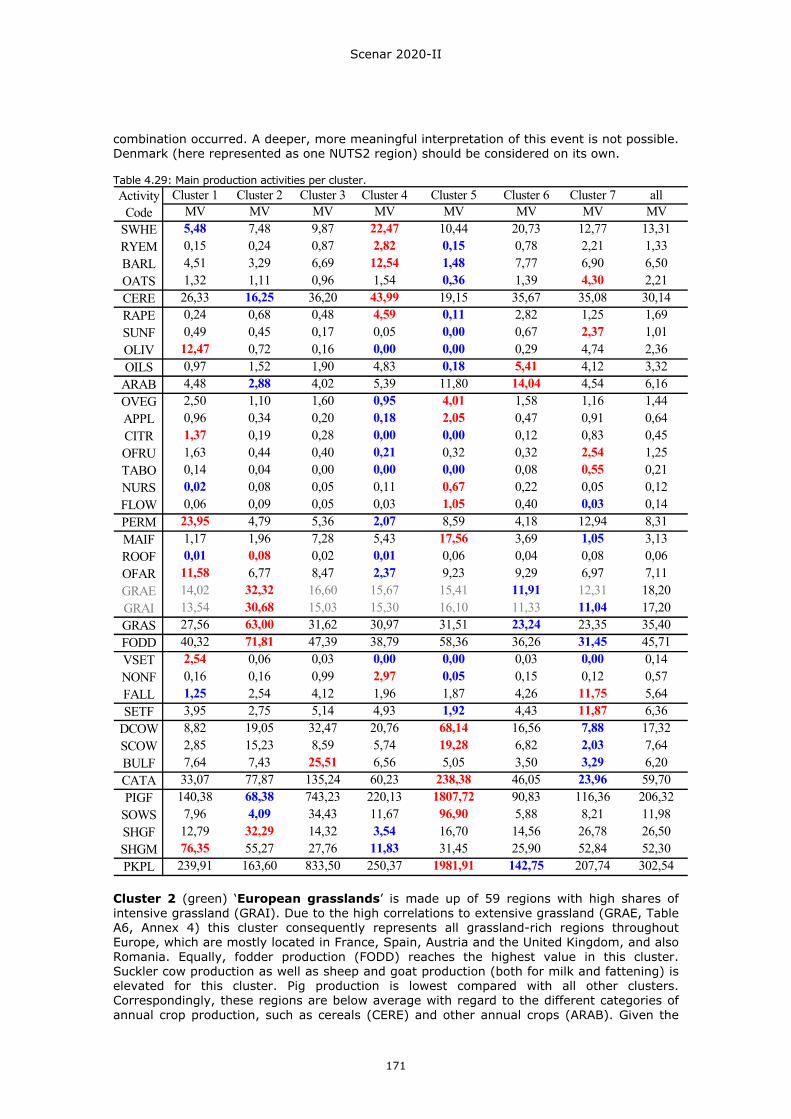
Scenar 2020-II

171

combination occurred. A deeper, more meaningful interpretation of this event is not possible. Denmark (here represented as one NUTS2 region) should be considered on its own. Table 4.29: Main production activities per cluster.

MV MV MV MV MV MV MV MVSWHE 5,48 7,48 9,87 22,47 10,44 20,73 12,77 13,31RYEM 0,15 0,24 0,87 2,82 0,15 0,78 2,21 1,33BARL 4,51 3,29 6,69 12,54 1,48 7,77 6,90 6,50OATS 1,32 1,11 0,96 1,54 0,36 1,39 4,30 2,21CERE 26,33 16,25 36,20 43,99 19,15 35,67 35,08 30,14RAPE 0,24 0,68 0,48 4,59 0,11 2,82 1,25 1,69SUNF 0,49 0,45 0,17 0,05 0,00 0,67 2,37 1,01OLIV 12,47 0,72 0,16 0,00 0,00 0,29 4,74 2,36OILS 0,97 1,52 1,90 4,83 0,18 5,41 4,12 3,32

ARAB 4,48 2,88 4,02 5,39 11,80 14,04 4,54 6,16OVEG 2,50 1,10 1,60 0,95 4,01 1,58 1,16 1,44APPL 0,96 0,34 0,20 0,18 2,05 0,47 0,91 0,64CITR 1,37 0,19 0,28 0,00 0,00 0,12 0,83 0,45OFRU 1,63 0,44 0,40 0,21 0,32 0,32 2,54 1,25TABO 0,14 0,04 0,00 0,00 0,00 0,08 0,55 0,21NURS 0,02 0,08 0,05 0,11 0,67 0,22 0,05 0,12FLOW 0,06 0,09 0,05 0,03 1,05 0,40 0,03 0,14PERM 23,95 4,79 5,36 2,07 8,59 4,18 12,94 8,31MAIF 1,17 1,96 7,28 5,43 17,56 3,69 1,05 3,13ROOF 0,01 0,08 0,02 0,01 0,06 0,04 0,08 0,06OFAR 11,58 6,77 8,47 2,37 9,23 9,29 6,97 7,11GRAE 14,02 32,32 16,60 15,67 15,41 11,91 12,31 18,20GRAI 13,54 30,68 15,03 15,30 16,10 11,33 11,04 17,20GRAS 27,56 63,00 31,62 30,97 31,51 23,24 23,35 35,40FODD 40,32 71,81 47,39 38,79 58,36 36,26 31,45 45,71VSET 2,54 0,06 0,03 0,00 0,00 0,03 0,00 0,14NONF 0,16 0,16 0,99 2,97 0,05 0,15 0,12 0,57FALL 1,25 2,54 4,12 1,96 1,87 4,26 11,75 5,64SETF 3,95 2,75 5,14 4,93 1,92 4,43 11,87 6,36

DCOW 8,82 19,05 32,47 20,76 68,14 16,56 7,88 17,32SCOW 2,85 15,23 8,59 5,74 19,28 6,82 2,03 7,64BULF 7,64 7,43 25,51 6,56 5,05 3,50 3,29 6,20CATA 33,07 77,87 135,24 60,23 238,38 46,05 23,96 59,70PIGF 140,38 68,38 743,23 220,13 1807,72 90,83 116,36 206,32

SOWS 7,96 4,09 34,43 11,67 96,90 5,88 8,21 11,98SHGF 12,79 32,29 14,32 3,54 16,70 14,56 26,78 26,50SHGM 76,35 55,27 27,76 11,83 31,45 25,90 52,84 52,30PKPL 239,91 163,60 833,50 250,37 1981,91 142,75 207,74 302,54

allActivity Code

Cluster 4 Cluster 5 Cluster 6 Cluster 7Cluster 1 Cluster 2 Cluster 3

Cluster 2 (green) ‘European grasslands’ is made up of 59 regions with high shares of intensive grassland (GRAI). Due to the high correlations to extensive grassland (GRAE, Table A6, Annex 4) this cluster consequently represents all grassland-rich regions throughout Europe, which are mostly located in France, Spain, Austria and the United Kingdom, and also Romania. Equally, fodder production (FODD) reaches the highest value in this cluster. Suckler cow production as well as sheep and goat production (both for milk and fattening) is elevated for this cluster. Pig production is lowest compared with all other clusters. Correspondingly, these regions are below average with regard to the different categories of annual crop production, such as cereals (CERE) and other annual crops (ARAB). Given the

Scenar 2020-II

172

overall trends in livestock production growth, as outlined in Section 3.4.1, these regions can make use of the market opportunities created by macro-economic drivers only to a small degree, and experience the impact of global competition and meat imports (Section 3.5.2). With regard to farm economics, this may have dramatic effects on the overall farm income, although the regions are beneficiaries of e.g. rural development policies, especially those dedicated to fodder activities (see Table 3.4, Section 3.6.1). Cluster 3 (violet) ‘Indoor beef production’ is the smallest cluster, consisting of only six regions that are characterised by an above average share in bull fattening (BULF). Likewise, production of cattle, but also pigs, poultry and other animals, is mostly high. Cattle are kept indoors with arable fodder production (MAIF + ROOF + OFAR) rather than being kept outdoors in grazing systems (GRAS below average). The regions form three coherent areas in Italy, Germany and Ireland. With respect to the macro-economic trends of increased global competition on the beef meat markets, these regions are likely to continue further specialisation of production. Cluster 4 (yellow) ‘Biofuel production’ has a total of 33 regions, showing the highest involvement in non-food production on set-aside (NONF). All regions are located in Germany, which suggests that this specialisation may be an effect of national policies. This cluster also shows the highest production of rape seed (RAPE); cereals production is also strong, especially soft wheat (SWHE), barley (BARL) and rye (RYEM) production. In addition, this cluster is characterised by lowest shares in fodder production on arable land (MAIF+ROOF+OFAR), production of vegetables, fruits and other perennials (PERM), as well as sheep and goat production, either for fattening or milk production (SHGM + SHGF). Altogether, this cluster contains all regions that are strongly engaged in biomass production for renewable energies. Cluster 5 (turquoise) ‘Intensive specialised production’ comprises nine regions with above average shares in pig fattening and pig breeding (PIGF+SOWS). The regions have a clear geographical orientation towards north-western maritime climate and are located in Belgium, the Netherlands and France. Cattle production is also very strong, and this also holds true for poultry and laying hens production. Furthermore, the regions of this cluster show an above average share of fodder production on arable land (MAIF+ROOF+OFAR). Consequently, this cluster holds all regions characterised by intensive livestock and production, especially with respect to pig production. Regions within this cluster obviously profit from the widening market opportunities created by increasing meat consumption as described in Section 3.5.2. In addition, production of vegetables (OVEG), fruits (APPL), trees and shrubs (NURS) as well as flowers (FLOW) is most pronounced in this cluster, while non-food production on set-aside land (NONF) is lowest compared with all other clusters. Economic effects at farm level are hence expected to be positive, regarding both the projected income increases for vegetables and permanent crops (Table 3.3, Section 3.6.1) and the price increase expected for pig meat (Table 3.2, Section 3.5.1). Cluster 6 (red) ‘Intensive crop farming’ includes 34 regions that show high production activities in the category of oil seeds (OILS) and other annual crops (ARAB). Cereal (CERE) production is also above average. Furthermore, for this cluster a below average share of grassland farming (GRAI and GRAE) can be observed. Therefore, this cluster represents those regions where intensive arable farming is prevalent, sometimes combined with livestock production (mixed farming). Actually, this cluster has many similarities in the expression of variables with cluster 4 ‘biofuel production’, except that in cluster 6 the ‘non-food’ variable is nearly irrelevant. The regions are scattered throughout Europe, with regions located in Belgium, the Netherlands, France, Austria, Sweden, United Kingdom, Greece, Czech Republic, Estonia and Slovakia. It can be assumed that the increased cereal and oilseed production as outlined in Section 3.5.2 occurs in these regions. Cluster 7 (blue) ‘Selected farming’ is characterised by an above average share of fallow land (FALL), that is arable land maintained under minimum standards for maintaining land under good agricultural and environmental conditions (GAEC) as formulated in the Council Regulation No. 1782/2003 instituting cross compliance. The average share of this type of land-use activity is nearly 12% of the total UAA. Altogether, 73 regions form this cluster and make it the largest and most heterogeneous one. Most regions of this cluster are located in

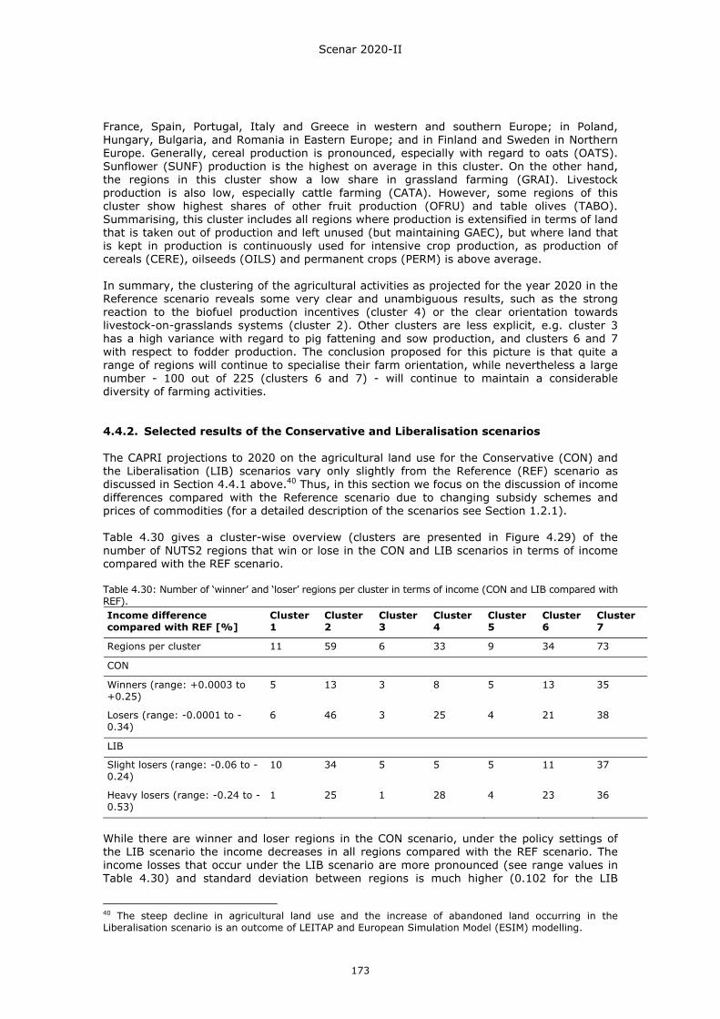
Scenar 2020-II

173

France, Spain, Portugal, Italy and Greece in western and southern Europe; in Poland, Hungary, Bulgaria, and Romania in Eastern Europe; and in Finland and Sweden in Northern Europe. Generally, cereal production is pronounced, especially with regard to oats (OATS). Sunflower (SUNF) production is the highest on average in this cluster. On the other hand, the regions in this cluster show a low share in grassland farming (GRAI). Livestock production is also low, especially cattle farming (CATA). However, some regions of this cluster show highest shares of other fruit production (OFRU) and table olives (TABO). Summarising, this cluster includes all regions where production is extensified in terms of land that is taken out of production and left unused (but maintaining GAEC), but where land that is kept in production is continuously used for intensive crop production, as production of cereals (CERE), oilseeds (OILS) and permanent crops (PERM) is above average. In summary, the clustering of the agricultural activities as projected for the year 2020 in the Reference scenario reveals some very clear and unambiguous results, such as the strong reaction to the biofuel production incentives (cluster 4) or the clear orientation towards livestock-on-grasslands systems (cluster 2). Other clusters are less explicit, e.g. cluster 3 has a high variance with regard to pig fattening and sow production, and clusters 6 and 7 with respect to fodder production. The conclusion proposed for this picture is that quite a range of regions will continue to specialise their farm orientation, while nevertheless a large number - 100 out of 225 (clusters 6 and 7) - will continue to maintain a considerable diversity of farming activities. 4.4.2. Selected results of the Conservative and Liberalisation scenarios The CAPRI projections to 2020 on the agricultural land use for the Conservative (CON) and the Liberalisation (LIB) scenarios vary only slightly from the Reference (REF) scenario as discussed in Section 4.4.1 above.40 Thus, in this section we focus on the discussion of income differences compared with the Reference scenario due to changing subsidy schemes and prices of commodities (for a detailed description of the scenarios see Section 1.2.1). Table 4.30 gives a cluster-wise overview (clusters are presented in Figure 4.29) of the number of NUTS2 regions that win or lose in the CON and LIB scenarios in terms of income compared with the REF scenario. Table 4.30: Number of ‘winner’ and ‘loser’ regions per cluster in terms of income (CON and LIB compared with REF). Income difference compared with REF [%]

Cluster 1

Cluster 2

Cluster 3

Cluster 4

Cluster 5

Cluster 6

Cluster 7

Regions per cluster 11 59 6 33 9 34 73

CON

Winners (range: +0.0003 to +0.25)

5 13 3 8 5 13 35

Losers (range: -0.0001 to -0.34)

6 46 3 25 4 21 38

LIB

Slight losers (range: -0.06 to -0.24)

10 34 5 5 5 11 37

Heavy losers (range: -0.24 to -0.53)

1 25 1 28 4 23 36

While there are winner and loser regions in the CON scenario, under the policy settings of the LIB scenario the income decreases in all regions compared with the REF scenario. The income losses that occur under the LIB scenario are more pronounced (see range values in Table 4.30) and standard deviation between regions is much higher (0.102 for the LIB

40 The steep decline in agricultural land use and the increase of abandoned land occurring in the Liberalisation scenario is an outcome of LEITAP and European Simulation Model (ESIM) modelling.

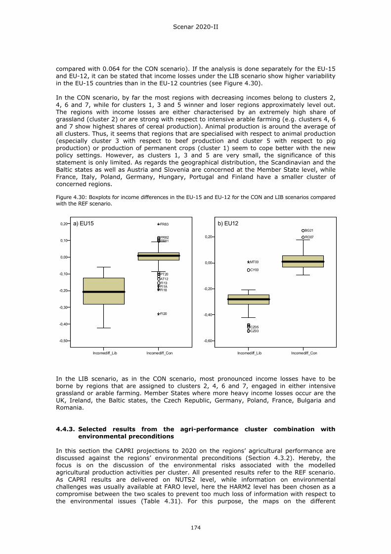
Scenar 2020-II

174

compared with 0.064 for the CON scenario). If the analysis is done separately for the EU-15 and EU-12, it can be stated that income losses under the LIB scenario show higher variability in the EU-15 countries than in the EU-12 countries (see Figure 4.30). In the CON scenario, by far the most regions with decreasing incomes belong to clusters 2, 4, 6 and 7, while for clusters 1, 3 and 5 winner and loser regions approximately level out. The regions with income losses are either characterised by an extremely high share of grassland (cluster 2) or are strong with respect to intensive arable farming (e.g. clusters 4, 6 and 7 show highest shares of cereal production). Animal production is around the average of all clusters. Thus, it seems that regions that are specialised with respect to animal production (especially cluster 3 with respect to beef production and cluster 5 with respect to pig production) or production of permanent crops (cluster 1) seem to cope better with the new policy settings. However, as clusters 1, 3 and 5 are very small, the significance of this statement is only limited. As regards the geographical distribution, the Scandinavian and the Baltic states as well as Austria and Slovenia are concerned at the Member State level, while France, Italy, Poland, Germany, Hungary, Portugal and Finland have a smaller cluster of concerned regions. Figure 4.30: Boxplots for income differences in the EU-15 and EU-12 for the CON and LIB scenarios compared with the REF scenario.

Incomediff_Lib Incomediff_Con

-0,50

-0,40

-0,30

-0,20

-0,10

0,00

0,10

0,20

FI13AT12PT20

FR81FR82

FI20

FI18FI1A

FR83

Incomediff_Lib Incomediff_Con

-0,60

-0,40

-0,20

0,00

0,20

CZ03CZ05

CY00

RO07

BG21

MT00

a) EU15 b) EU12

Incomediff_Lib Incomediff_Con

-0,50

-0,40

-0,30

-0,20

-0,10

0,00

0,10

0,20

FI13AT12PT20

FR81FR82

FI20

FI18FI1A

FR83

Incomediff_Lib Incomediff_Con

-0,60

-0,40

-0,20

0,00

0,20

CZ03CZ05

CY00

RO07

BG21

MT00

a) EU15 b) EU12

In the LIB scenario, as in the CON scenario, most pronounced income losses have to be borne by regions that are assigned to clusters 2, 4, 6 and 7, engaged in either intensive grassland or arable farming. Member States where more heavy income losses occur are the UK, Ireland, the Baltic states, the Czech Republic, Germany, Poland, France, Bulgaria and Romania. 4.4.3. Selected results from the agri-performance cluster combination with

environmental preconditions In this section the CAPRI projections to 2020 on the regions’ agricultural performance are discussed against the regions’ environmental preconditions (Section 4.3.2). Hereby, the focus is on the discussion of the environmental risks associated with the modelled agricultural production activities per cluster. All presented results refer to the REF scenario. As CAPRI results are delivered on NUTS2 level, while information on environmental challenges was usually available at FARO level, here the HARM2 level has been chosen as a compromise between the two scales to prevent too much loss of information with respect to the environmental issues (Table 4.31). For this purpose, the maps on the different

Scenar 2020-II

175

environmental issues were upscaled from FARO to HARM2-level and CAPRI results and results of the cluster analysis were downscaled from NUTS2 to HARM2. Table 4.31: Number of regions per cluster at NUTS2 and at HARM2 level. Cluster

1 Cluster 2

Cluster 3

Cluster 4

Cluster 5

Cluster 6

Cluster 7

Total

NUTS2 Regions per cluster

11 59 6 33 9 34 73 225

HARM2 Regions per cluster

59 174 28 33 12 78 275 659

4.4.3.1. Risk of water scarcity due to restrained water storage in soil

With respect to water availability for agricultural land use, the capacity of soils to maintain water is one of the important factors together with the climate conditions of rainfall and temperature that together shape the natural site conditions. Hence, the indicator of soils with a high share of limited water availability was used to characterise environmental conditions vulnerable to intensive agricultural land use. And, as crops typical of intensive land use and sensitive to water scarcity, the focus was placed on the activity group of permanent crops such as citrus, fruits, berries and vines. Thus, the share of permanent crops (PERM) was chosen as an indicator for the risk assessment. Table 4.32 shows how many regions that are challenged by the risk of limited available water capacity in soils are at the same time characterised by higher shares of permanent crop production dependent on irrigation. The regions are presented in Figure 4.31. Table 4.32: HARM2 regions with high shares of soils with limited available water capacity (> 15.2%) and permanent crop production (> 10%). Country Cluster 1 Cluster 2 Cluster 3 Cluster 4 Cluster 5 Cluster 6 Cluster 7 ∑ Total no. 174 78 275 659 Spain 1 20 21 (out of 50) Greece 3 1 20 24 (out of 51) ∑ 0 4 0 0 0 1 40 45

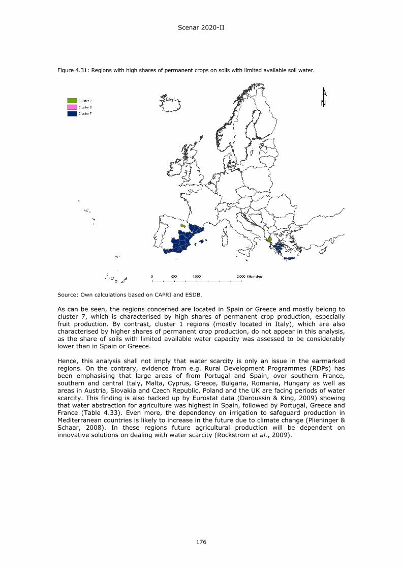
Scenar 2020-II

176

Figure 4.31: Regions with high shares of permanent crops on soils with limited available soil water.

Source: Own calculations based on CAPRI and ESDB. As can be seen, the regions concerned are located in Spain or Greece and mostly belong to cluster 7, which is characterised by high shares of permanent crop production, especially fruit production. By contrast, cluster 1 regions (mostly located in Italy), which are also characterised by higher shares of permanent crop production, do not appear in this analysis, as the share of soils with limited available water capacity was assessed to be considerably lower than in Spain or Greece. Hence, this analysis shall not imply that water scarcity is only an issue in the earmarked regions. On the contrary, evidence from e.g. Rural Development Programmes (RDPs) has been emphasising that large areas of from Portugal and Spain, over southern France, southern and central Italy, Malta, Cyprus, Greece, Bulgaria, Romania, Hungary as well as areas in Austria, Slovakia and Czech Republic, Poland and the UK are facing periods of water scarcity. This finding is also backed up by Eurostat data (Daroussin & King, 2009) showing that water abstraction for agriculture was highest in Spain, followed by Portugal, Greece and France (Table 4.33). Even more, the dependency on irrigation to safeguard production in Mediterranean countries is likely to increase in the future due to climate change (Plieninger & Schaar, 2008). In these regions future agricultural production will be dependent on innovative solutions on dealing with water scarcity (Rockstrom et al., 2009).

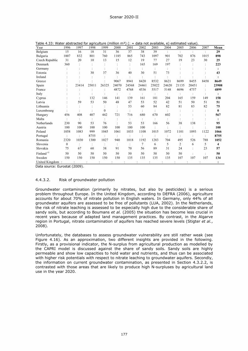
Scenar 2020-II

177

Table 4.33: Water abstracted for agriculture (million m³) (: = data not available, e) estimated value). Year 1996 1997 1998 1999 2000 2001 2002 2003 2004 2005 2006 2007 MeanBelgium 15 16 18 31 36 37 38 39 : : : : 29Bulgaria 1007 832 801 760 1185 865 743 1097 901 702 876 1015 898Czech Republic 31 20 10 13 15 12 19 77 27 19 23 30 25Denmark 360 : : : : : 165 169 197 : : : 223Germany : : : : : : : : : : : : :Estonia : : 30 37 36 40 30 51 73 : : : 43Ireland : : : : : : : : : : : : :Greece : : : : 9067 8941 8420 8532 8621 8699 8455 8458 8649Spain : 23414 25011 26325 24070 24568 24461 25022 24620 21135 20451 : 23908France : : : : 4872 4768 4536 5517 5148 4696 4757 : 4899Italy : : : : : : : : : : : : :Cyprus : : 132 146 141 139 161 181 204 165 159 149 158Latvia : 59 53 50 48 47 53 52 42 51 50 51 51Lithuania : : : : : 53 60 84 82 81 83 82 75Luxembourg : : : 0 : : : : : : : : 0Hungary 456 408 407 442 721 716 680 670 602 : : : 567Malta : : : : : : : : : : : : :Netherlands 230 90 53 76 : 53 53 166 56 38 138 : 95Austria 100 100 100 100 100 100 100 : : : : : 100Poland 1058 1083 999 1045 1061 1033 1108 1015 1072 1101 1093 1122 1066Portugal : : 8755 : : : : : : : : : 8755Romania 2320 1030 1300 1027 940 1018 1192 1283 704 495 526 788 1052Slovenia 0 : : : : : 7 6 5 2 6 5 4Slovakia 75 67 60 38 91 70 56 89 31 24 : 23 57Finland e) 50 50 50 50 50 50 50 50 50 50 : : 50Sweden 150 150 150 150 150 135 135 135 135 107 107 107 134United Kingdom : : : : : : : : : : : : : Data source: Eurostat (2009). 4.4.3.2. Risk of groundwater pollution

Groundwater contamination (primarily by nitrates, but also by pesticides) is a serious problem throughout Europe. In the United Kingdom, according to DEFRA (2006), agriculture accounts for about 70% of nitrate pollution in English waters. In Germany, only 44% of all groundwater aquifers are assessed to be free of pollutants (LUA, 2002). In the Netherlands, the risk of nitrate leaching is assessed to be especially high due to the considerable share of sandy soils, but according to Boumans et al. (2005) the situation has become less crucial in recent years because of adapted land management practices. By contrast, in the Algarve region in Portugal, nitrate contamination of aquifers has reached severe levels (Stigter et al., 2008). Unfortunately, the databases to assess groundwater vulnerability are still rather weak (see Figure 4.16). As an approximation, two different insights are provided in the following. Firstly, as a provisional indicator, the N-surplus from agricultural production as modelled by the CAPRI model is discussed against the share of sandy soils. Sandy soils are highly permeable and show low capacities to hold water and nutrients, and thus can be associated with higher risk potentials with respect to nitrate leaching to groundwater aquifers. Secondly, the information on current groundwater contamination, as presented in Section 4.3.2.2, is contrasted with those areas that are likely to produce high N-surpluses by agricultural land use in the year 2020.

Scenar 2020-II

178

Table 4.34: HARM2 regions challenged by high shares of sandy soils (> 34.68%) and high N-surpluses by agricultural production (> 100 kg/ha). Country Cluster 1 Cluster 2 Cluster 3 Cluster 4 Cluster 5 Cluster 6 Cluster 7 ∑ Total 59 28 33 12 78 275 659 Belgium 3 3 (out of 9) Germany 4 6 10 (out of 36) Denmark 10 10 (out of 12) Italy 11 11 (out of 95) Nether-lands

2 4 1 7 (out of 12)

United Kingdom

3 1 4 (out of 26)

∑ 10 5 15 6 7 2 0 45 By far the most regions with high shares of sandy soils and at the same time high surpluses of nitrogen in agricultural production can be found in Italy, Germany, Denmark and the Netherlands (Figure 4.32). Clusters that have an elevated number of regions with a high N-surplus are ‘indoor beef production’, ‘biofuel production’ and ‘intensive specialised production’, which are all characterised by a considerable number of livestock (cattle, pigs, poultry and other animals). Additionally, all regions of Denmark are comprised in this selection, which are part of but not typical for cluster 1 (Table 4.34). Figure 4.32: Regions with farming-generated high N-surpluses on sandy soils.

In order to improve the understanding of the groundwater pollution risk, recent information on levels of nitrate contamination has also been taken into account. The analysis revealed that 184 out of 839 FARO regions are affected by a high (> 51mg/l) or a very high level (> 101mg/l) of nitrate concentration in groundwater. These current state findings constitute a weakness with regard to further agricultural land use: appropriate measures and practices have to be undertaken to reduce possible current nitrate emissions and to prevent further charges. This is valid for all regions concerned, but special attention has to be paid to those regions where specialised and intensive production methods prevail, as in clusters 3 (indoor

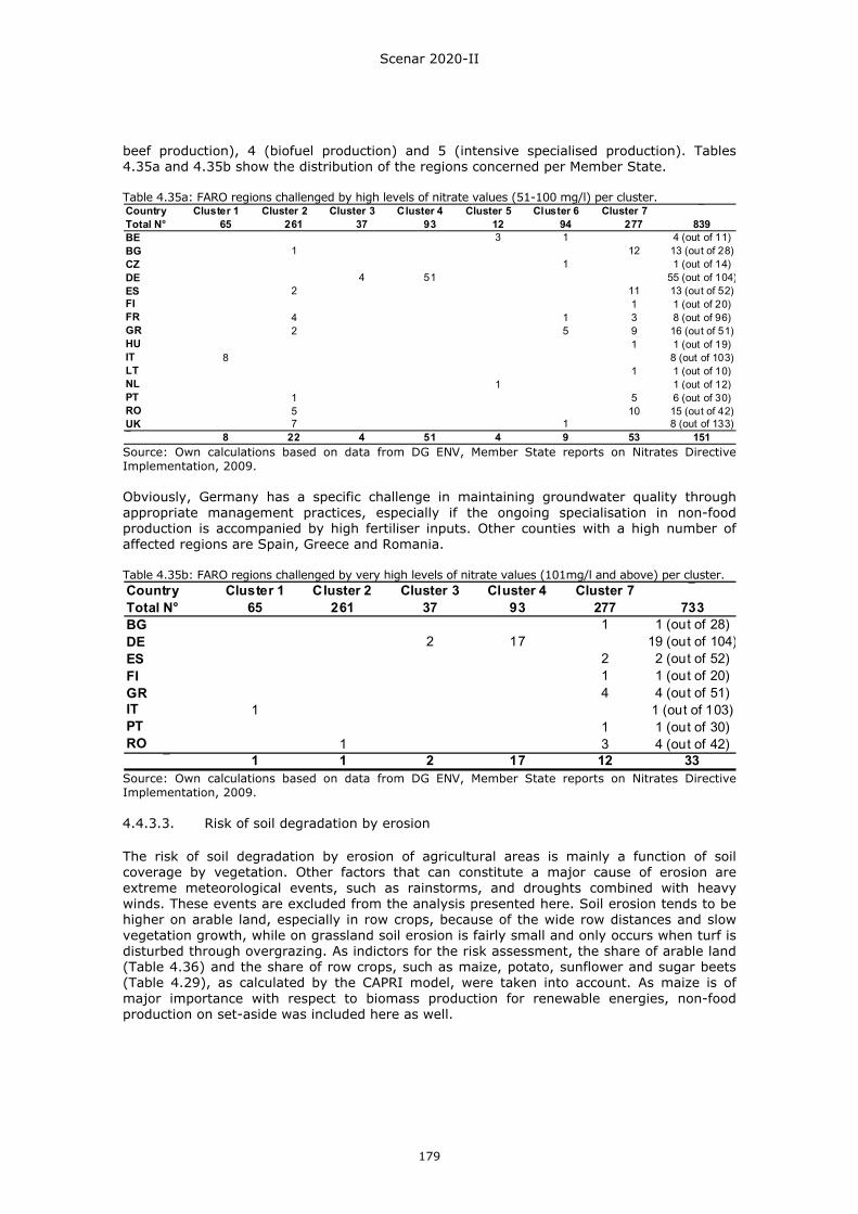
Scenar 2020-II

179

beef production), 4 (biofuel production) and 5 (intensive specialised production). Tables 4.35a and 4.35b show the distribution of the regions concerned per Member State. Table 4.35a: FARO regions challenged by high levels of nitrate values (51-100 mg/l) per cluster. Country Cluster 1 Cluster 2 Cluster 3 Cluster 4 Cluster 5 Cluster 6 Cluster 7 ⎯Total N° 65 261 37 93 12 94 277 839BE 3 1 4 (out of 11)BG 1 12 13 (out of 28)CZ 1 1 (out of 14)DE 4 51 55 (out of 104)ES 2 11 13 (out of 52)FI 1 1 (out of 20)FR 4 1 3 8 (out of 96)GR 2 5 9 16 (out of 51)HU 1 1 (out of 19)IT 8 8 (out of 103)LT 1 1 (out of 10)NL 1 1 (out of 12)PT 1 5 6 (out of 30)RO 5 10 15 (out of 42)UK 7 1 8 (out of 133)⎯ 8 22 4 51 4 9 53 151 Source: Own calculations based on data from DG ENV, Member State reports on Nitrates Directive Implementation, 2009. Obviously, Germany has a specific challenge in maintaining groundwater quality through appropriate management practices, especially if the ongoing specialisation in non-food production is accompanied by high fertiliser inputs. Other counties with a high number of affected regions are Spain, Greece and Romania. Table 4.35b: FARO regions challenged by very high levels of nitrate values (101mg/l and above) per cluster. Country Cluster 1 Cluster 2 Cluster 3 Cluster 4 Cluster 7 ⎯Total N° 65 261 37 93 277 733BG 1 1 (out of 28)DE 2 17 19 (out of 104)ES 2 2 (out of 52)FI 1 1 (out of 20)GR 4 4 (out of 51)IT 1 1 (out of 103)PT 1 1 (out of 30)RO 1 3 4 (out of 42)

⎯ 1 1 2 17 12 33 Source: Own calculations based on data from DG ENV, Member State reports on Nitrates Directive Implementation, 2009. 4.4.3.3. Risk of soil degradation by erosion

The risk of soil degradation by erosion of agricultural areas is mainly a function of soil coverage by vegetation. Other factors that can constitute a major cause of erosion are extreme meteorological events, such as rainstorms, and droughts combined with heavy winds. These events are excluded from the analysis presented here. Soil erosion tends to be higher on arable land, especially in row crops, because of the wide row distances and slow vegetation growth, while on grassland soil erosion is fairly small and only occurs when turf is disturbed through overgrazing. As indictors for the risk assessment, the share of arable land (Table 4.36) and the share of row crops, such as maize, potato, sunflower and sugar beets (Table 4.29), as calculated by the CAPRI model, were taken into account. As maize is of major importance with respect to biomass production for renewable energies, non-food production on set-aside was included here as well.

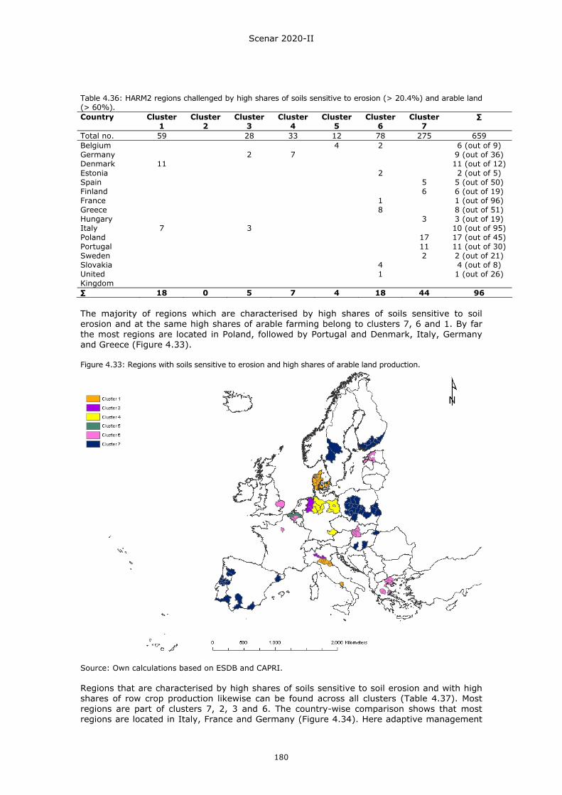
Scenar 2020-II

180

Table 4.36: HARM2 regions challenged by high shares of soils sensitive to erosion (> 20.4%) and arable land (> 60%). Country Cluster

1 Cluster

2 Cluster

3 Cluster

4 Cluster

5 Cluster

6 Cluster

7 ∑

Total no. 59 28 33 12 78 275 659 Belgium 4 2 6 (out of 9) Germany 2 7 9 (out of 36) Denmark 11 11 (out of 12) Estonia 2 2 (out of 5) Spain 5 5 (out of 50) Finland 6 6 (out of 19) France 1 1 (out of 96) Greece 8 8 (out of 51) Hungary 3 3 (out of 19) Italy 7 3 10 (out of 95) Poland 17 17 (out of 45) Portugal 11 11 (out of 30) Sweden 2 2 (out of 21) Slovakia 4 4 (out of 8) United Kingdom

1 1 (out of 26)

∑ 18 0 5 7 4 18 44 96 The majority of regions which are characterised by high shares of soils sensitive to soil erosion and at the same high shares of arable farming belong to clusters 7, 6 and 1. By far the most regions are located in Poland, followed by Portugal and Denmark, Italy, Germany and Greece (Figure 4.33). Figure 4.33: Regions with soils sensitive to erosion and high shares of arable land production.

Source: Own calculations based on ESDB and CAPRI. Regions that are characterised by high shares of soils sensitive to soil erosion and with high shares of row crop production likewise can be found across all clusters (Table 4.37). Most regions are part of clusters 7, 2, 3 and 6. The country-wise comparison shows that most regions are located in Italy, France and Germany (Figure 4.34). Here adaptive management

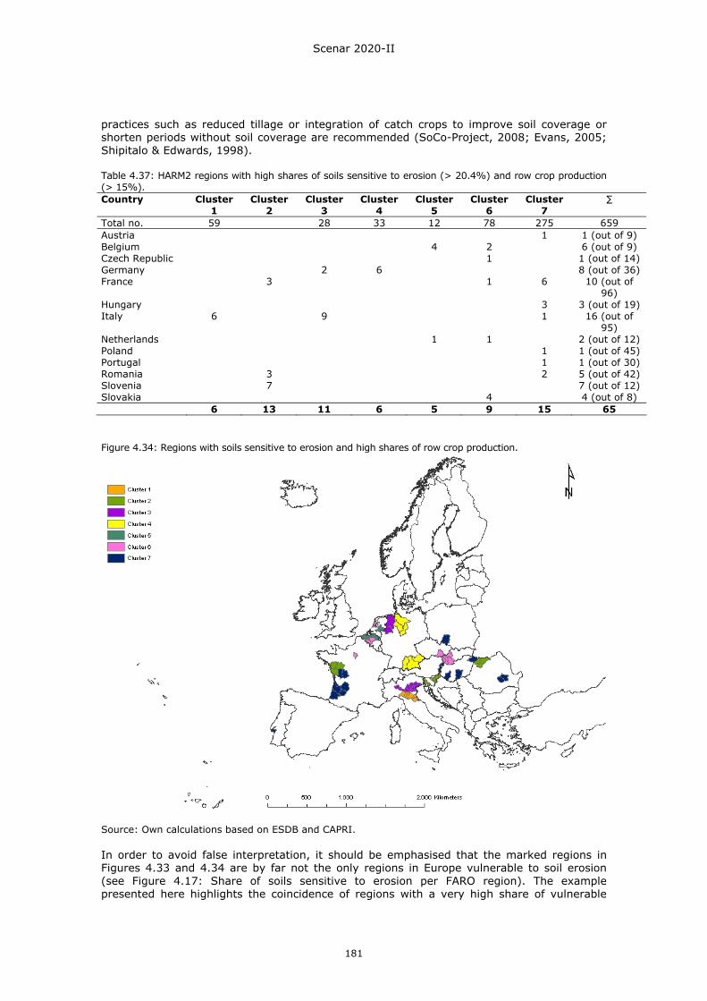
Scenar 2020-II

181

practices such as reduced tillage or integration of catch crops to improve soil coverage or shorten periods without soil coverage are recommended (SoCo-Project, 2008; Evans, 2005; Shipitalo & Edwards, 1998). Table 4.37: HARM2 regions with high shares of soils sensitive to erosion (> 20.4%) and row crop production (> 15%). Country Cluster

1 Cluster

2 Cluster

3 Cluster

4 Cluster

5 Cluster

6 Cluster

7 ∑

Total no. 59 28 33 12 78 275 659 Austria 1 1 (out of 9) Belgium 4 2 6 (out of 9) Czech Republic 1 1 (out of 14) Germany 2 6 8 (out of 36) France 3 1 6 10 (out of

96) Hungary 3 3 (out of 19) Italy 6 9 1 16 (out of

95) Netherlands 1 1 2 (out of 12) Poland 1 1 (out of 45) Portugal 1 1 (out of 30) Romania 3 2 5 (out of 42) Slovenia 7 7 (out of 12) Slovakia 4 4 (out of 8) 6 13 11 6 5 9 15 65 Figure 4.34: Regions with soils sensitive to erosion and high shares of row crop production.

Source: Own calculations based on ESDB and CAPRI. In order to avoid false interpretation, it should be emphasised that the marked regions in Figures 4.33 and 4.34 are by far not the only regions in Europe vulnerable to soil erosion (see Figure 4.17: Share of soils sensitive to erosion per FARO region). The example presented here highlights the coincidence of regions with a very high share of vulnerable

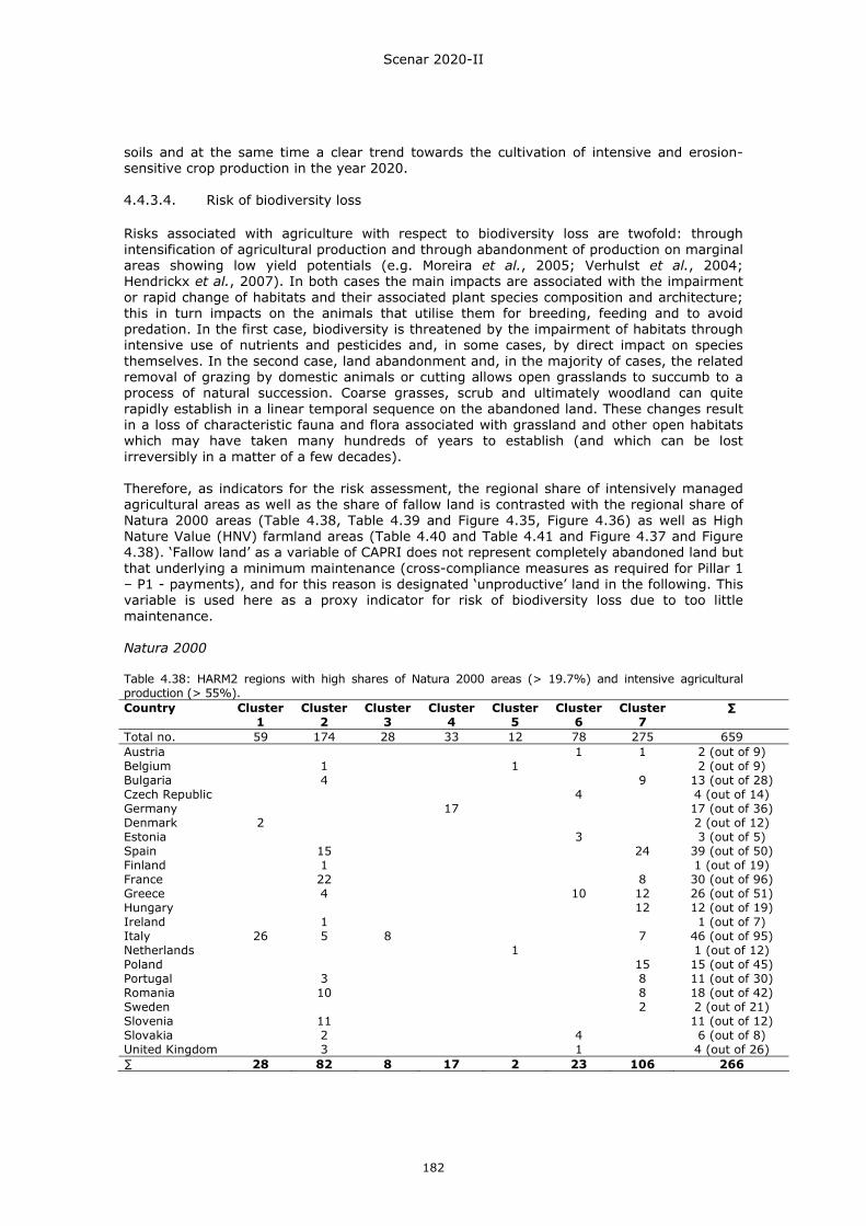
Scenar 2020-II

182

soils and at the same time a clear trend towards the cultivation of intensive and erosion-sensitive crop production in the year 2020. 4.4.3.4. Risk of biodiversity loss

Risks associated with agriculture with respect to biodiversity loss are twofold: through intensification of agricultural production and through abandonment of production on marginal areas showing low yield potentials (e.g. Moreira et al., 2005; Verhulst et al., 2004; Hendrickx et al., 2007). In both cases the main impacts are associated with the impairment or rapid change of habitats and their associated plant species composition and architecture; this in turn impacts on the animals that utilise them for breeding, feeding and to avoid predation. In the first case, biodiversity is threatened by the impairment of habitats through intensive use of nutrients and pesticides and, in some cases, by direct impact on species themselves. In the second case, land abandonment and, in the majority of cases, the related removal of grazing by domestic animals or cutting allows open grasslands to succumb to a process of natural succession. Coarse grasses, scrub and ultimately woodland can quite rapidly establish in a linear temporal sequence on the abandoned land. These changes result in a loss of characteristic fauna and flora associated with grassland and other open habitats which may have taken many hundreds of years to establish (and which can be lost irreversibly in a matter of a few decades). Therefore, as indicators for the risk assessment, the regional share of intensively managed agricultural areas as well as the share of fallow land is contrasted with the regional share of Natura 2000 areas (Table 4.38, Table 4.39 and Figure 4.35, Figure 4.36) as well as High Nature Value (HNV) farmland areas (Table 4.40 and Table 4.41 and Figure 4.37 and Figure 4.38). ‘Fallow land’ as a variable of CAPRI does not represent completely abandoned land but that underlying a minimum maintenance (cross-compliance measures as required for Pillar 1 – P1 - payments), and for this reason is designated ‘unproductive’ land in the following. This variable is used here as a proxy indicator for risk of biodiversity loss due to too little maintenance. Natura 2000 Table 4.38: HARM2 regions with high shares of Natura 2000 areas (> 19.7%) and intensive agricultural production (> 55%). Country Cluster

1 Cluster

2 Cluster

3 Cluster

4 Cluster

5 Cluster

6 Cluster

7 ∑

Total no. 59 174 28 33 12 78 275 659 Austria 1 1 2 (out of 9) Belgium 1 1 2 (out of 9) Bulgaria 4 9 13 (out of 28) Czech Republic 4 4 (out of 14) Germany 17 17 (out of 36) Denmark 2 2 (out of 12) Estonia 3 3 (out of 5) Spain 15 24 39 (out of 50) Finland 1 1 (out of 19) France 22 8 30 (out of 96) Greece 4 10 12 26 (out of 51) Hungary 12 12 (out of 19) Ireland 1 1 (out of 7) Italy 26 5 8 7 46 (out of 95) Netherlands 1 1 (out of 12) Poland 15 15 (out of 45) Portugal 3 8 11 (out of 30) Romania 10 8 18 (out of 42) Sweden 2 2 (out of 21) Slovenia 11 11 (out of 12) Slovakia 2 4 6 (out of 8) United Kingdom 3 1 4 (out of 26) ∑ 28 82 8 17 2 23 106 266

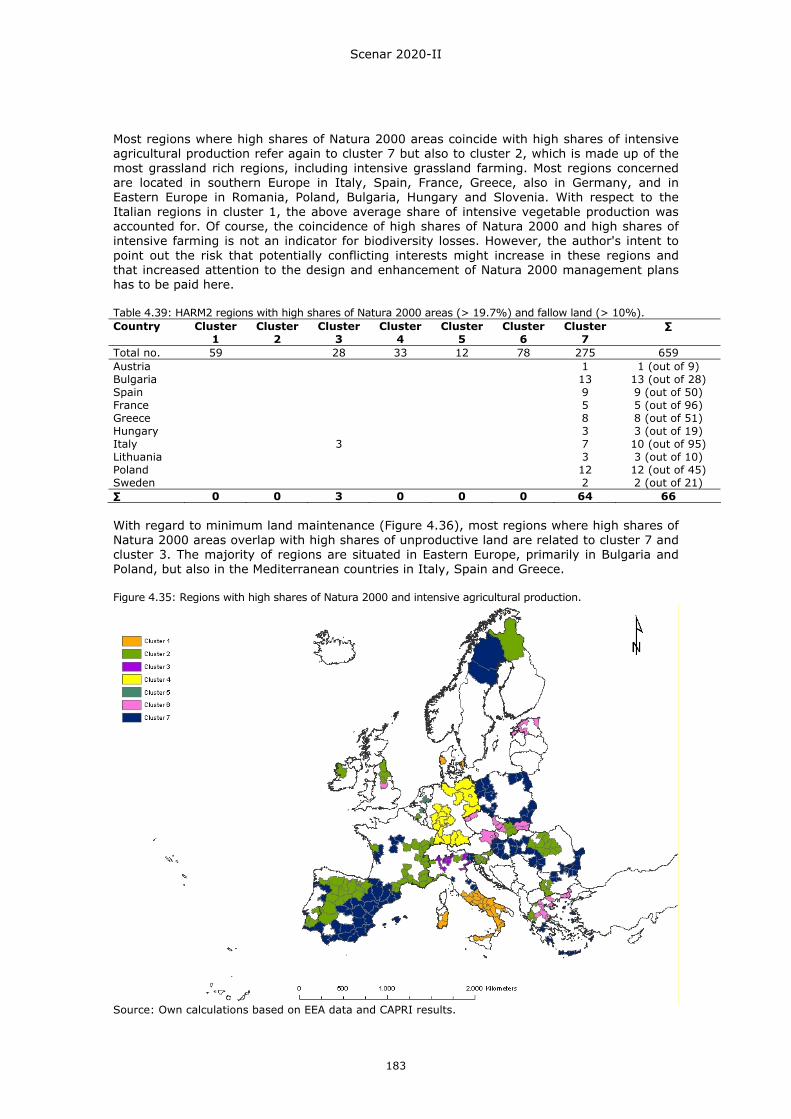
Scenar 2020-II

183

Most regions where high shares of Natura 2000 areas coincide with high shares of intensive agricultural production refer again to cluster 7 but also to cluster 2, which is made up of the most grassland rich regions, including intensive grassland farming. Most regions concerned are located in southern Europe in Italy, Spain, France, Greece, also in Germany, and in Eastern Europe in Romania, Poland, Bulgaria, Hungary and Slovenia. With respect to the Italian regions in cluster 1, the above average share of intensive vegetable production was accounted for. Of course, the coincidence of high shares of Natura 2000 and high shares of intensive farming is not an indicator for biodiversity losses. However, the author's intent to point out the risk that potentially conflicting interests might increase in these regions and that increased attention to the design and enhancement of Natura 2000 management plans has to be paid here. Table 4.39: HARM2 regions with high shares of Natura 2000 areas (> 19.7%) and fallow land (> 10%). Country Cluster

1 Cluster

2 Cluster

3 Cluster

4 Cluster

5 Cluster

6 Cluster

7 ∑

Total no. 59 28 33 12 78 275 659 Austria 1 1 (out of 9) Bulgaria 13 13 (out of 28) Spain 9 9 (out of 50) France 5 5 (out of 96) Greece 8 8 (out of 51) Hungary 3 3 (out of 19) Italy 3 7 10 (out of 95) Lithuania 3 3 (out of 10) Poland 12 12 (out of 45) Sweden 2 2 (out of 21) ∑ 0 0 3 0 0 0 64 66 With regard to minimum land maintenance (Figure 4.36), most regions where high shares of Natura 2000 areas overlap with high shares of unproductive land are related to cluster 7 and cluster 3. The majority of regions are situated in Eastern Europe, primarily in Bulgaria and Poland, but also in the Mediterranean countries in Italy, Spain and Greece. Figure 4.35: Regions with high shares of Natura 2000 and intensive agricultural production.

Source: Own calculations based on EEA data and CAPRI results.

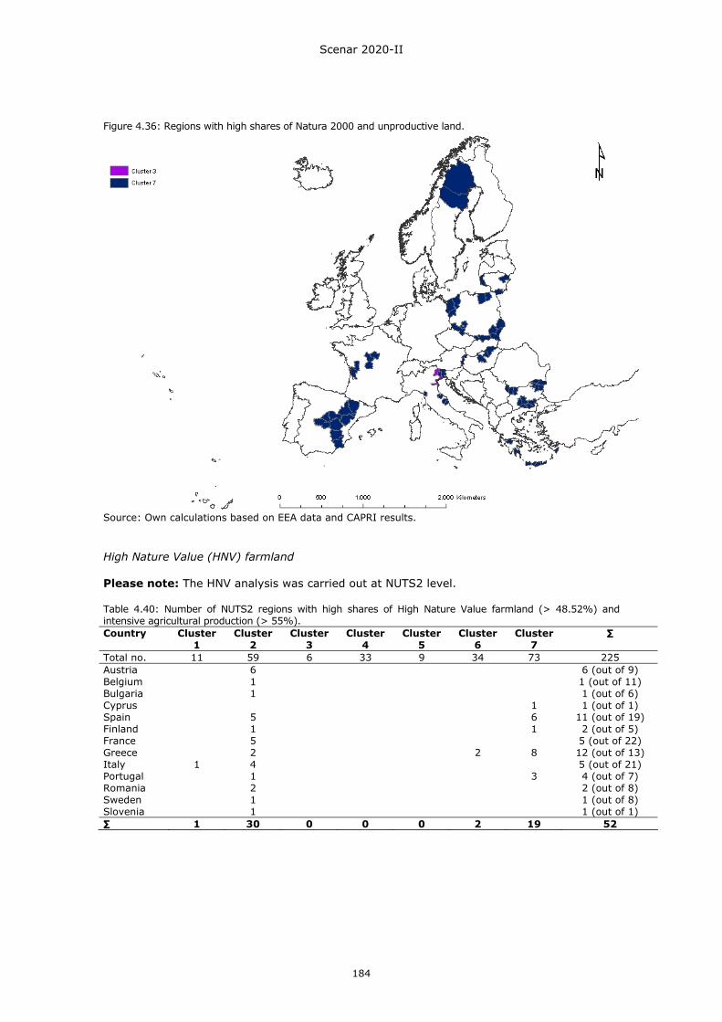
Scenar 2020-II

184

Figure 4.36: Regions with high shares of Natura 2000 and unproductive land.

Source: Own calculations based on EEA data and CAPRI results. High Nature Value (HNV) farmland Please note: The HNV analysis was carried out at NUTS2 level. Table 4.40: Number of NUTS2 regions with high shares of High Nature Value farmland (> 48.52%) and intensive agricultural production (> 55%). Country Cluster

1 Cluster

2 Cluster

3 Cluster

4 Cluster

5 Cluster

6 Cluster

7 ∑

Total no. 11 59 6 33 9 34 73 225 Austria 6 6 (out of 9) Belgium 1 1 (out of 11) Bulgaria 1 1 (out of 6) Cyprus 1 1 (out of 1) Spain 5 6 11 (out of 19) Finland 1 1 2 (out of 5) France 5 5 (out of 22) Greece 2 2 8 12 (out of 13) Italy 1 4 5 (out of 21) Portugal 1 3 4 (out of 7) Romania 2 2 (out of 8) Sweden 1 1 (out of 8) Slovenia 1 1 (out of 1) ∑ 1 30 0 0 0 2 19 52

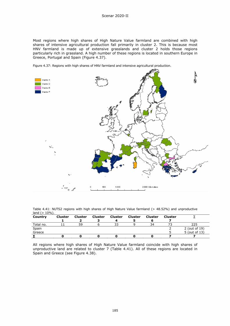
Scenar 2020-II

185

Most regions where high shares of High Nature Value farmland are combined with high shares of intensive agricultural production fall primarily in cluster 2. This is because most HNV farmland is made up of extensive grasslands and cluster 2 holds those regions particularly rich in grassland. A high number of these regions is located in southern Europe in Greece, Portugal and Spain (Figure 4.37). Figure 4.37: Regions with high shares of HNV farmland and intensive agricultural production.

Table 4.41: NUTS2 regions with high shares of High Nature Value farmland (> 48.52%) and unproductive land (> 10%). Country Cluster

1 Cluster

2 Cluster

3 Cluster

4 Cluster

5 Cluster

6 Cluster

7 ∑

Total no. 11 59 6 33 9 34 73 225 Spain 2 2 (out of 19) Greece 5 5 (out of 13) ∑ 0 0 0 0 0 0 7 7 All regions where high shares of High Nature Value farmland coincide with high shares of unproductive land are related to cluster 7 (Table 4.41). All of these regions are located in Spain and Greece (see Figure 4.38).

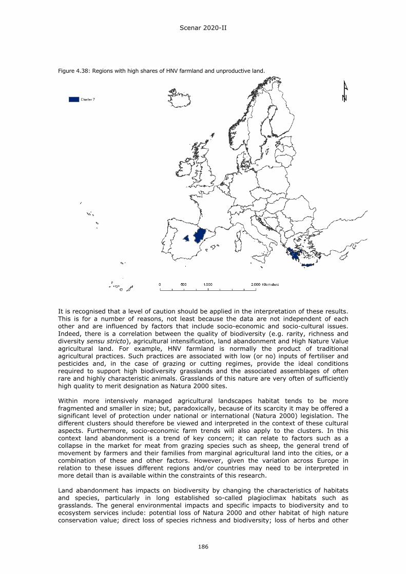
Scenar 2020-II

186

Figure 4.38: Regions with high shares of HNV farmland and unproductive land.

It is recognised that a level of caution should be applied in the interpretation of these results. This is for a number of reasons, not least because the data are not independent of each other and are influenced by factors that include socio-economic and socio-cultural issues. Indeed, there is a correlation between the quality of biodiversity (e.g. rarity, richness and diversity sensu stricto), agricultural intensification, land abandonment and High Nature Value agricultural land. For example, HNV farmland is normally the product of traditional agricultural practices. Such practices are associated with low (or no) inputs of fertiliser and pesticides and, in the case of grazing or cutting regimes, provide the ideal conditions required to support high biodiversity grasslands and the associated assemblages of often rare and highly characteristic animals. Grasslands of this nature are very often of sufficiently high quality to merit designation as Natura 2000 sites. Within more intensively managed agricultural landscapes habitat tends to be more fragmented and smaller in size; but, paradoxically, because of its scarcity it may be offered a significant level of protection under national or international (Natura 2000) legislation. The different clusters should therefore be viewed and interpreted in the context of these cultural aspects. Furthermore, socio-economic farm trends will also apply to the clusters. In this context land abandonment is a trend of key concern; it can relate to factors such as a collapse in the market for meat from grazing species such as sheep, the general trend of movement by farmers and their families from marginal agricultural land into the cities, or a combination of these and other factors. However, given the variation across Europe in relation to these issues different regions and/or countries may need to be interpreted in more detail than is available within the constraints of this research. Land abandonment has impacts on biodiversity by changing the characteristics of habitats and species, particularly in long established so-called plagioclimax habitats such as grasslands. The general environmental impacts and specific impacts to biodiversity and to ecosystem services include: potential loss of Natura 2000 and other habitat of high nature conservation value; direct loss of species richness and biodiversity; loss of herbs and other

Scenar 2020-II

187

special plants that are collected by local people for medicinal purposes; loss of cultural heritage, as these areas have significant links to socio-cultural practice, transhumance, etc; loss of soil structure and the potential for increased erosion in certain circumstances which will also reduce the capacity for carbon sequestration; loss of ecotourism opportunities as these areas are particularly attractive for walking, hiking and nature tours, not least because they provide the opportunity to view a wider landscape; they may often be characteristic to the extent that people associate with them psychologically and they provide a source of local pride in relation to some of their characteristic species. Particularly in the face of changing climatic conditions, land abandonment can lead to heightened fire risk. On the positive side, land abandonment can increase the potential for carbon sequestration and reduce the speed of surface water run-off in storm conditions. The implications of this for thinking about the future are clear. Much of the land in Europe which presently has a value for wildlife, including those areas with national or international (Natura 2000) designations, is managed extensively using traditional agricultural practices. Without incentives for this management to continue it is likely that land abandonment will take place, with the above-mentioned consequences for biodiversity. 4.4.3.5. Greenhouse gas emission risks from agriculture

Agriculture is seen as one of the emitters of greenhouse gases to the atmosphere (Smith, 2004) and is thus challenged to reduce the emissions (Brown et al., 2008; Rounsevell et al., 2006). Therefore, three options for climate change mitigation are applicable: reduction of direct emission, reduction of indirect emissions and enhancement of carbon sequestration in soils by stimulating the sink function of soils (Belyea & Malmer, 2004). Direct emissions include emissions that are released by produced ruminants, relate to consumption of fuel and electricity, or are emitted from soils. Indirect emission in the first place stems from the manufacturing of inputs, machinery and equipment employed in the production process. Here we used two indicators for direct emissions. As soil-borne emissions are particularly high if soils rich in organic carbon are under arable farming, as a first indicator the regions’ share of organic soils was compared to share of arable land (Table 4.42). As a second indicator we generated an overview of the average number of ruminants (only cattle farming was taken into account) per hectare for each cluster and country based on the CAPRI outcomes (Table 4.43). Table 4.42: HARM2 regions with high shares of organic soils (11.7%) and arable land (> 50%). Country Cluster

1 Cluster

2 Cluster

3 Cluster

4 Cluster

5 Cluster

6 Cluster

7 ∑

Belgium 2 2 (out of 9) Germany 2 5 7 (out of 36)Estonia 3 3 (out of 5) Finland 3 3 (out of 19)France 1 1 (out of 96)Hungary 1 1 (out of 19)Latvia 4 4 (out of 6) Netherlands 3 3 6 (out of 12)Poland 4 4 (out of 45)United Kingdom 1 1 (out of 26) 0 1 2 5 5 7 12 32 Most regions where higher shares of organic soils coincide with large areas under arable farming can be found in Germany, the Netherlands, Poland, Latvia, Estonia and Finland (Figure 4.39).

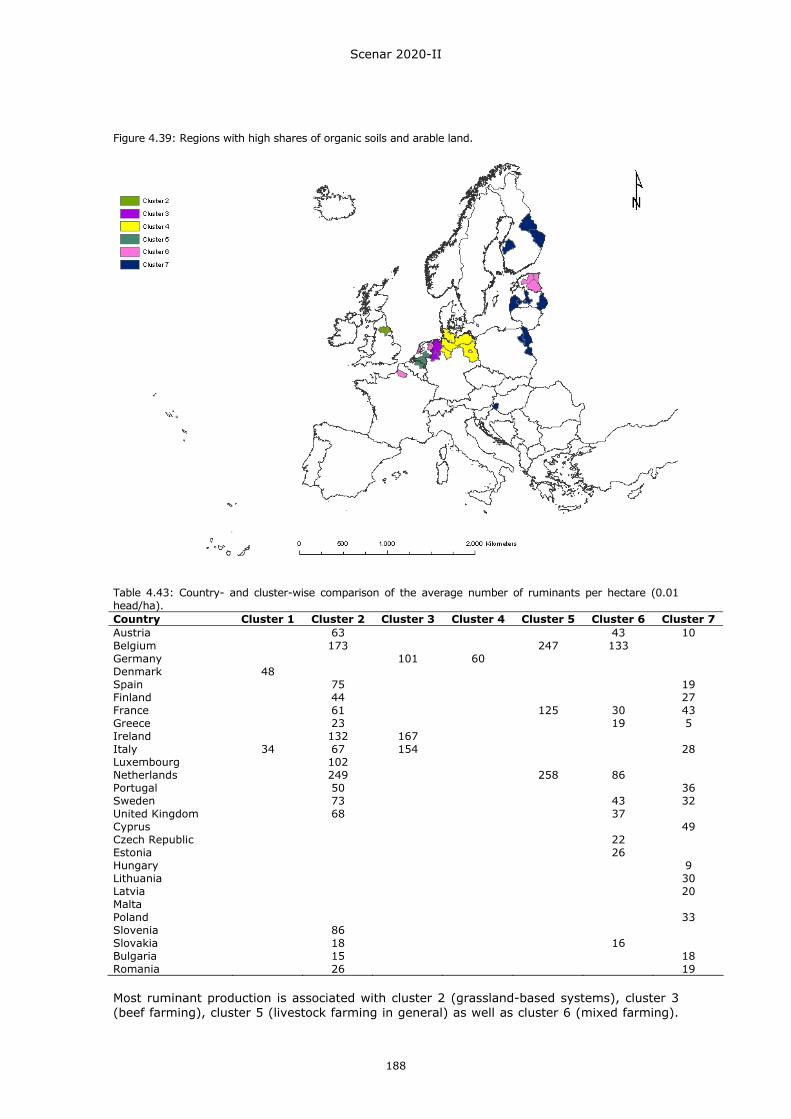
Scenar 2020-II

188

Figure 4.39: Regions with high shares of organic soils and arable land.

Table 4.43: Country- and cluster-wise comparison of the average number of ruminants per hectare (0.01 head/ha). Country Cluster 1 Cluster 2 Cluster 3 Cluster 4 Cluster 5 Cluster 6 Cluster 7 Austria 63 43 10 Belgium 173 247 133 Germany 101 60 Denmark 48 Spain 75 19 Finland 44 27 France 61 125 30 43 Greece 23 19 5 Ireland 132 167 Italy 34 67 154 28 Luxembourg 102 Netherlands 249 258 86 Portugal 50 36 Sweden 73 43 32 United Kingdom 68 37 Cyprus 49 Czech Republic 22 Estonia 26 Hungary 9 Lithuania 30 Latvia 20 Malta Poland 33 Slovenia 86 Slovakia 18 16 Bulgaria 15 18 Romania 26 19 Most ruminant production is associated with cluster 2 (grassland-based systems), cluster 3 (beef farming), cluster 5 (livestock farming in general) as well as cluster 6 (mixed farming).

Scenar 2020-II

189

Cattle farming also occurs for a number of countries in cluster 7, but concentrations in terms of animal head per hectare are rather small compared with clusters 2 and 6. 4.4.4. Selected environmental results from alternative scenario modelling While the previous section contrasted typical regional reactions in the field of agricultural land use with present environmental conditions (mostly in terms of vulnerabilities), this section presents environmental consequences of the different scenarios with regard to agricultural emissions, particularly nitrogen surplus. Although the modelling of environmental indicators in CAPRI has limitations, it gives an indication of how the economic incentives included in the Conservative CAP scenario and the Liberalisation scenario might affect the emissions to the environment. At the outset, it should also be noted that only a limited number of environmental indicators are included in CAPRI (nitrogen and phosphate surplus, ammonia and GHG emissions). Hence, the modelling delivers only a partial picture of the true effects of the scenarios on the environment, landscape, biodiversity, etc. The main objective of the EU Nitrates Directive (European Commission, 1991) and the EU Water Framework Directive (European Commission, 2000) is to improve the chemical and ecological condition of European bodies of water. It is changing the way farmers are managing and applying manure, and therefore it is expected that a significant decrease in nitrogen should be obtained over the next few years, in particular in regions currently designated as nitrogen vulnerable zones. So far, however, this is not fully taken into account in CAPRI. This makes it difficult to predict the changes in different environmental indicators going from 2002 to 2020. Therefore Table 4.44 only presents percentage differences between the 2020 Reference scenario and the two alternative scenarios. Table 4.44 shows that the effect of agricultural production on the selected environmental indicators averaged for the EU-27 increases in the Conservative CAP scenario, while the effect of agricultural production on the selected environmental indicators decreases in the Liberalisation scenario. The increase of the nitrogen surplus in the Conservative CAP scenario is explained by the coupled suckler cow payments in some countries and regions and by the sharp decrease of second pillar (P2) payments that reduce the number of farms with environmentally friendly and extensive production systems. The decrease in the nitrate surplus in the Liberalisation scenario as compared with the Reference scenario is explained by decreased agricultural production. Table 4.44: Percentage changes in environmental indicators; Conservative CAP and Liberalisation scenarios as compared with 2020 Reference scenario; average EU-27.

Conservative Liberalisation

Compared with Reference

Kg per ha Kg per ha

Nitrogen surplus 0.8% -1.3%

Phosphate surplus 1.0% -1.3%

Ammonium output 0.1% -1.6%

CH4 total emissions 0.0% -3.6%

Global warming emissions41 0.4% -2.8% Source: CAPRI results.

41 Methane (GCH4) and nitrous oxide (GN2O) emissions measured in CO2 equivalents.

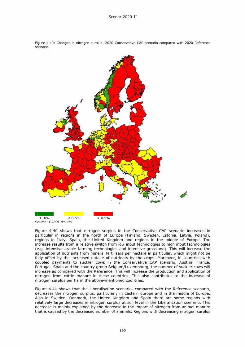
Scenar 2020-II

190

Figure 4.40: Changes in nitrogen surplus: 2020 Conservative CAP scenario compared with 2020 Reference scenario.

< 0% < 0.5% > 0.5%

Source: CAPRI results. Figure 4.40 shows that nitrogen surplus in the Conservative CAP scenario increases in particular in regions in the north of Europe (Finland, Sweden, Estonia, Latvia, Poland), regions in Italy, Spain, the United Kingdom and regions in the middle of Europe. The increase results from a relative switch from low input technologies to high input technologies (e.g. intensive arable farming technologies and intensive grassland). This will increase the application of nutrients from mineral fertilisers per hectare in particular, which might not be fully offset by the increased uptake of nutrients by the crops. Moreover, in countries with coupled payments to suckler cows in the Conservative CAP scenario, Austria, France, Portugal, Spain and the country group Belgium/Luxembourg, the number of suckler cows will increase as compared with the Reference. This will increase the production and application of nitrogen from cattle manure in these countries. This also contributes to the increase of nitrogen surplus per ha in the above-mentioned countries. Figure 4.41 shows that the Liberalisation scenario, compared with the Reference scenario, decreases the nitrogen surplus, particularly in Eastern Europe and in the middle of Europe. Also in Sweden, Denmark, the United Kingdom and Spain there are some regions with relatively large decreases in nitrogen surplus at soil level in the Liberalisation scenario. This decrease is mainly explained by the decrease in the import of nitrogen from animal manure that is caused by the decreased number of animals. Regions with decreasing nitrogen surplus

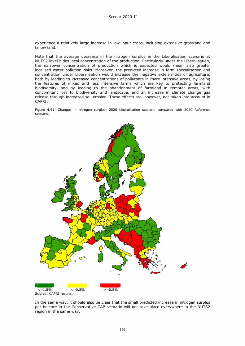
Scenar 2020-II

191

experience a relatively large increase in low input crops, including extensive grassland and fallow land. Note that the average decrease in the nitrogen surplus in the Liberalisation scenario at NUTS2 level hides local concentration of the production. Particularly under the Liberalisation, the narrower concentration of production which is expected would mean also greater localised water pollution risks. Moreover, the predicted increase in farm specialisation and concentration under Liberalisation would increase the negative externalities of agriculture, both by leading to increased concentrations of pollutants in more intensive areas, by losing the features of mixed and less intensive farms which are key to protecting farmland biodiversity, and by leading to the abandonment of farmland in remoter areas, with concomitant loss to biodiversity and landscape, and an increase in climate change gas release through increased soil erosion. These effects are, however, not taken into account in CAPRI. Figure 4.41: Changes in nitrogen surplus: 2020 Liberalisation scenario compared with 2020 Reference scenario.

< -1.5% < -0.5% > -0.5%

Source: CAPRI results. In the same way, it should also be clear that the small predicted increase in nitrogen surplus per hectare in the Conservative CAP scenario will not take place everywhere in the NUTS2 region in the same way.

Scenar 2020-II

192

4.4.5. Conclusions on agricultural performance A first interesting finding of the agricultural land-use analysis is that the differences in production activities between the three scenarios were so small that the clustering results were the same for all three scenarios. These results are in line with the assumption that through the mid-term review and the Health Check reforms, land use has now become fully decoupled in the logic underlying the attribution of financial support to farmers; land use depends partly on natural and structural site conditions and mostly on agricultural markets and comparative advantages. Obviously, policy effects are not strong enough – or they are counterbalanced under the assumptions made here – to noticeably vary land-use patterns all over Europe. This, of course, is not true for farm income - a difference that consequently has structural effects that can only approximately be appreciated based on the given modelling approach. Further research and especially refinement of the modelling approach would substantially improve the depth of interpretation. The typical regional reactions in 2020’s agricultural land use reveal a continuation of the current situation: a trend towards specialisation, on the one hand (cluster 4, cluster 3, cluster 5 and cluster 1), and a maintenance of various types of mixed farming in combination with a certain share of unproductive land, on the other (cluster 7, cluster 6). This share of roughly 11–12% unproductive land (on average) under minimum maintenance in 73 out of 225 regions (cluster 7) is a distinctive characteristic of the sector’s ongoing structural change. This share of land bears the risk of becoming truly abandoned of any management if not seized by appropriate policy measures. Another interesting finding is that, obviously, national policies such as the German biofuel legislation or those shaping specific P2 schemes (e.g. in cluster 1) have a direct impact on land-use patterns. Although in the future, national policies might be different from what has been assumed here, the example shows that this level of political intervention has a recognisable impact. Further research and especially refinement of the modelling approach are necessary to allow for a more differentiated analysis and conclusions. The contrasting of the future agricultural land-use patterns with a selection of environmental conditions gives a rather patchy picture. This is partially due to the severe shortcomings in the data availability at the desired level of regional disaggregation. On the other hand, this general picture indicates that environmental challenges are obviously very diverse throughout the EU-27 regions. The general finding is that the clusters are not uniform with respect to the environmental impacts. With respect to most indicators, regions from different clusters reveal threatening features. More specifically, a combinatory analysis has to be viewed with caution. Especially the attempt to capture the environmental significance of agricultural land use for soil-borne water and groundwater has met its limits: • Soil-borne water availability is truly restricted in several Southern and Eastern European

regions and might be a limiting factor for sensitive agricultural cultures such as vegetables. However, neither climatic conditions (rainfall, temperature) nor the availability of irrigation water could be included in the analysis.

• Groundwater pollution by intensive agricultural production is already currently a severe

problem in some regions. The modelling results indicate the continuation of intensive agriculture for quite a number of regions. However, the possibility of overcoming nitrogen leaching by e.g. appropriate agricultural practices has not been taken into account in this analysis.

The consideration of the soil erosion risk is based on more extensive data. The findings show that the risk of soil erosion in the EU-27 tends to be higher on arable land in general (96 out of 659 regions are concerned) and in regions with row crop production, which is sensitive to erosion (65 out of 659 regions are concerned), Again, the analysis does not reveal a salient cluster or a dominant spatial entity, but a patchy picture all over Europe.

Scenar 2020-II

193

With regard to biodiversity conservation and the management of valuable ecosystems on and bordering farm land, the challenges are of considerable spatial relevance as 266 regions out of 659 have a high share of Natura 2000 areas and a projected high share of intensively managed farmland. Here, public attention on the effective establishment and enforcement of Natura 2000 management plans is necessary to ensure the integrity of habitats. The coincidence of projected high shares of intensive farming and High Nature Value farmland areas is less frequent, with 52 out of 225 regions. Nevertheless, this issue also has to be watched carefully in the future, as here a direct overlapping of areas and hence conflicting land-use targets are even more likely to happen. The interpretation of the environmental indicators that have been drawn from the modelling of alternative scenarios gives an indication of how the economic incentives included in the Conservative CAP scenario and the Liberalisation scenario might affect the emissions to the environment. In certain circumstances, the considerable structural change that is likely to come under the full liberalisation of agricultural activity could have variable environmental effects, as increasing specialisation will occur in some regions and more extensive agricultural land management in others. Particular attention should be paid to the environmental consequences linked to the abandonment of land management in marginal areas.

4.5. Overall discussion and conclusions on the SWOT analysis

1) With regard to the general approach of this SWOT analysis that is based on projected

data-sets and modelling outputs, the conclusions of Scenar 2020-I still hold true, that by this ‘top-down outsider perspective’ only half of the view is taken and that the regions’ insider appraisal is, of course, missing in this document.

2) Also, it should be emphasised that no overall aggregation of the data is recommended because of (i) the heterogeneity of the data provenance, and (ii) the differences in the spatial/administrative level of data disaggregation. Additionally, it should be emphasised that more conceptual research is needed to overcome conceptual gaps for cross-sectional comparisons.

3) The considerable regional diversity that was a finding in Scenar 2020-I is not questioned

by Scenar 2020-II. The range in economic terms and with regard to agricultural structures has become larger, given that Bulgaria and Romania are included in this second analysis.

4) However, mainly because of weak data availability in some cases and uncertainties due

to the economic crisis, with respect to the economic projections in particular a cautious attitude has been adopted and, hence, the middle field of regions has become considerably larger. For example, out of 857 regions, 561 have slightly positive economic perspectives and expect a moderate employment growth (>0 to 0.5%).

5) With regard to the demographic development, the projected figures indicate a mixed

perspective for the EU-27’s regional areas, where altogether 422 regions have a negative and 435 regions a positive development direction. This relation corresponds fairly well to the proportions identified in Scenar 2020-I. Generally, the changes and trends in the EU-27 can be considered as moderate in comparison with trends in other world regions. Considering the national level, almost every country has at least one region with a positive trend. With regard to the OECD classification, strong rurality is not synonymous with negative demographic trends. However, it is equally obvious that rural regions in the eastern Member States and at the southern and northern borders of the EU are distinctly more marked by population decrease than Western Europe.

6) Aggregating demographic and economic trends, the general picture of the EU-27 regions’

socio-economic reactions in 2020 is that of rather small changes. Both population growth and decline as well as changes in employment growth range largely between -1 and

Scenar 2020-II

194

+1% annual change rate. Hence, without moderating the existing differences too much, a relative stability can be expected. Of course, the impacts of the current economic crisis are not included in the projective calculations and therefore cannot be assessed here. They might lead in some places to the accentuation of negative tendencies and trends.

7) Furthermore, the analysis shows that although all types of regions are represented all

over the EU-27, there is a difference between the EU-12 and the EU-15, with the more positive reactions in the old Member States. This finding again repeats findings of Scenar 2020-I. Hence, with regard to the opportunities in the service sector, it could be discussed whether emerging ‘strong’ regions and clusters in the EU-12, as well as in the southern parts of the EU-15, should be enhanced so that they can lead in the structural transformation towards more service sector orientation in support of employment creation.

8) There is no evidence that the EU-27 regions with an above average agricultural

employment are generally showing negative reactions. Thus, it is emphasised that rurality and agricultural vocation are not a sign of weak development perspectives. However, as the overall trend in the sector’s employment is declining (median sinks from 5.43% in 2004 to 3.05% in 2020), it cannot be counted on as a stabilising factor, either. Nevertheless, if employment-relevant policy measures are discussed within a rural development framework (as e.g. the third and the fourth axis of the EAFRD Regulation), then their objectives and possible impacts should be analysed and assessed before treating the general socio-economic performance of a region.

9) In contrast with Scenar 2020-I, the present study has developed an approach to tackle

the quality of life issue by the way of objective data that exceed pure economic figures. However, the analysis has been restricted to current-state data, and hence it has to be emphasised that there is no straight conceptual assumption about a linkage between current quality of life conditions and future socio-economic reactions of the regions. The findings of this current-state analysis reveal that the quality of life appraisal for 711 out of 857 regions scores zero (249 regions) or negative results (562 regions). This means that many regions exceed others by only one characteristic, while at the same time the other indicators remain below average (or all indicators are at average level). The group of positively scoring regions is small (comprising only 1/6 of all regions) as the coincidence of two or even three above average indicators is rather exceptional. Not surprisingly, in this group ‘most urban’ regions make up almost 50%. Nevertheless, the share of ‘most rural’ regions is larger than that of the ‘intermediate rural’ ones so that, again, rurality is not a denominator for low quality of life!

10) Methodologically, the Scenar 2020 quality of life assessment has yielded a first complex

presentation of the issue by integrating non-economic indicators, at a considerable level of spatial disaggregation. Further research is necessary to carefully confirm the assumptions of this promising approach and hereby increase its validity.

11) With regard to the future socio-economic perspectives of the EU-27 regions, the findings

of the quality of life assessment can be interpreted in terms of enforcing strengths or hindering weaknesses. From the cross-sectional analysis, it becomes obvious that regions with a weak socio-economic reaction in 2020 are also characterised by an average or low quality of life state today. Hence, with regard to the chosen parameters, it should not be expected that these types of regions will be in a position to significantly off-set quality of life potentials to counterbalance weak reactions in demographics and economic dynamics. Most rural regions are especially numerous in the group which has a low socio-economic performance and whose current quality of life conditions reveal the lowest averages of all groups except the natural capital. It could be assumed that these regions are facing an ‘accelerating economic development’ until 2020 and, hence, agricultural and other rural policies might be right to take care of the maintenance of the natural capital in this dynamic. Regions with a positive socio-economic perspective reveal mostly neutral to positive quality of life preconditions, and only 37 out of 287 belong to the ‘low’ category. Thus, we assume that an enforcement of current structures for future reactions can be expected.

Scenar 2020-II

195

12) While the analysis of socio-economic perspectives reveals a certain difference between the EU-15 and the EU-12, the clustering of the agricultural structures shows coherences for a north-western and a south-eastern distinction. The cross-sectional analysis of the present agri-structural conditions and the future socio-economic perspectives does not support the idea of an alignment between today’s strengths and weaknesses and the future, and also, no theoretical bases exist to back up such linkages. Hence, results should be taken as a hint for interpretation rather than as descriptions of possible futures, so that e.g. weak current agricultural structures (in terms of small-scale farming) may constitute future ballast for regions with an altogether weak socio-economic performance.

13) In summary, the clustering of the agricultural activities as projected for the year 2020 in

the Reference scenario reveals a continuation of the current situation: a distinctive trend towards specialised agricultural activities in roughly one-quarter of the regions, on the one hand, and, on the other hand, maintenance of various types of mixed and grazing livestock farming in combination with a certain share of unproductive land on the remaining three-quarters. (Note: the number of the regions does not reflect their spatial size.) Some dominant projected land-use patterns, such as grazing livestock farming and specialised meat production, are in line with current agricultural structures, while in large areas in Southern, Northern and Eastern Europe the overall picture remains rather vague.

14) With regard to the environmental risks that are related to the agricultural activities of the

Reference scenario, it can be stated that, although they are manifold, none dominates in spatial terms or with regard to a specific orientation of agricultural production. While the vulnerability of the water resources cannot be systematically appreciated on the basis of the available data, a cautious appreciation of the soil erosion risk through agriculture revealed that roughly 14% of the regions are concerned. The assessment of the regional sensitivity of biodiversity against agricultural practices presents more conceptual and methodological challenges as data availability and comparability are restricted. Here, improved data consistency of the High Nature Value (HNV) farmland indicator will be of great value for further research. High shares of regional land abandonment, as projected by the outcomes of the CAPRI modelling, constitute another factor that could have negative impacts on both the regional ecosystem qualities and the visual landscape amenities.

15) Further changes in environmental conditions that the agricultural sector has to deal with

in the future are the opportunities and risks related to climate change. In this study, only a few aspects have been taken into account, in particular those related to soil organic matter. On the one hand, the protection of the organic content of soils through appropriate farming practices will always be of high relevance, but especially in the regions with high peatland shares, as peaty soils are particularly vulnerable to erosion. On the other hand, the contribution to climate change mitigation by targeted storage of carbon in soils with low organic matter could constitute an option for the agricultural sector, and merits further investigation.

Scenar 2020-II

196

5. Synthesis: Preparing for change Because the Scenar 2020-II study is an extension of the initial study, the structure of the continuing investigation builds upon the conclusions previously obtained when working on Scenar 2020 in 2006, either refining them or challenging them. This synthesis of the update undertaken places the conclusions of the first study as a backdrop. Against this backdrop, in a second section six thematic axes are presented, and further developed in light of the major points from other recent similar literature. According to the perspective on the future of agriculture and the rural economy thus provided, the combined insights from the economic analysis of the agricultural sector and the regional SWOT analysis are developed in the third section. Conclusions are presented in the last section.

5.1. Conclusions from the initial Scenar 2020 study 1) Rural areas are not stable. Migration patterns are having a strong influence on the

economic framework of rural areas, and contrary forces are at work, leading to demographic out-migration and economic decline, or the reinforcement of the socio-economic dynamism. The distinction between rural and urban is becoming less clear in terms of principal activity being agriculture, for in many rural areas agriculture has a modest role in the generation of GVA even if it is the primary land use. This leads to rapid changes in land use, with the marginalisation of certain rural areas from all points of view. This risk is greatest along the eastern frontier of the EU. Where agriculture is decreasing as the primary land use, forestry is increasing in the eastern parts of the EU. The structural changes in agriculture are a long-term trend, but with the changes in the territorial dynamics of the EU following the enlargement with 12 new Member States, some regions are experiencing problems of accessibility to major centres of demand within the unified market space; this will also influence the regional response to commodity markets, and in turn will have a direct repercussion on the types and number of farms within a region.

2) Agriculture within the EU-27 is very diverse, and will change substantially by the 2020 time horizon. The historical distribution of farm structure is not going to remain: with farm sizes varying from one hectare to several thousand, and with economic viability no longer embracing the extremes in technical capacity that are represented by wide variations in educational background of the farming profession, the EU agricultural sector is undergoing and will continue to undergo major adjustment.

3) Growth in world agricultural markets will slow down. Although this conclusion might seem surprising after the recent experience of price peaks in many primary commodity markets, slowing population growth shifts the reason for increasing demand from population growth to the evolution of income per capita. How this evolution will proceed, originally forecast to be rapid and significant in developing and transition countries, is less obvious than previously. It is sure that past trends indicate that income growth, urbanisation and dietary diversification lead not only to additional demand but also to changes in the composition of food consumption, with a fast growing share of animal products. In the developed countries, the growth in food consumption is limited, and other social and economic factors will lead the regional shifts in agricultural commodity production. Technological innovations are occurring both in primary and intermediate commodity production processes and in the transport of goods, which enables a change in agricultural land availability and in market suppliers to occur at the global level. The consequences for cross-border trade remain an open question.

4) There are several distinct key trends in EU commodity markets up to the horizon of 2020. These are:

a) Increasing segmentation within the EU market because of the growing relative importance of transportation costs, as goods move further within an enlarged market area, a situation which would be enhanced by further liberalisation and enlargement.

Scenar 2020-II

197

b) Decline in cereal prices, in real terms, coupled with continuing increases in yield, will lead to a decrease in area required for their production; a reduced nominal rent value of land and lower feed costs are also part of the explanation.

c) The livestock market will undergo important restructuring, with a concentration on dairy production, poultry meat and pork meat production. The decline in beef production is partially a reflection of consumer preferences interrelated with trends in consumption and partially a result of trade factors. Increases in milk yield will reinforce the shrinking of the cattle herd, and this will have a direct repercussion on fodder requirements. The trend towards increased trade liberalisation will reinforce this general structural evolution.

d) In parallel with the increased resort to biofuels, oilseed production will shift towards the requirements for industrial use as opposed to food consumption. The area of oilseed production should increase, depending on trade regulations having an influence on the sourcing of ethanol.

5) Structural change process in agriculture is a long-term process that continues with or without policy changes. The long-term trend is dependent on many variables at the macro-economic level, which were outlined in the original report and are not repeated here. There are two consequences of this trend that are, nevertheless, important to highlight. First, there continues to be a surplus in agricultural labour that is partially hidden by refusal to leave the sector and that is partially a reason for structural unemployment in some areas where low-qualified industrial jobs are not available as an employment substitute. Second, out-migration for reasons of agricultural unemployment will particularly weaken the socio-economic potential of the eastern EU frontier and the north-west corner of the Iberian peninsula.

6) Policy change produces differentiated impact. There are two key remarks in this regard by which to underpin this point.

a) The reduction of border support (import tariffs and export subsidies) has a higher impact on agricultural production than the reduction of domestic income support. On the other hand, reducing domestic income support has a larger impact on farm income than the reduction of border support. This supports the view that a shift from border support to income support is less production distorting for a production/trade point of view and is better in terms of preserving a stable income for farmers.

b) The process of liberalisation has a greater impact on agricultural income than on agricultural production and land use; this fact consolidates the structural pressure throughout Europe to decrease labour in farming and to increase average farm size.

7) Within the limits of the foreseeable budget, the total amount of EU Rural Development support per farmer or per agricultural area is small in comparison with the regional GVA in the agricultural sector in most EU regions. Specified targeted policies might be effective to achieve the foreseen objectives in certain areas. Nevertheless, other drivers have a far greater impact on GVA, and will also influence the agricultural sector.

8) Productivity increase derived from technological innovation is an exogenous factor, from which new opportunities can be promoted through policy, but which will in any case evolve independently of policy. The case of biofuels is an example.

9) The major uncertainty with regard to all conclusions concerning the future of biofuels is the tightness of oil/energy markets. The impact of biofuels might be underestimated (and a food–fuel debate has since become a major policy agenda point).

10) The role of forestry in rural areas is not given enough attention. A long-term trend in afforestation is witnessed in several countries of the EU.

Scenar 2020-II

198

11) There are several environmental issues linked to agricultural land use, but in general the negative impacts of agricultural practice have been declining over time.

12) The effects of global warming will be increasingly evident in the period leading up to 2020, with direct consequences for the management of natural resources and for agricultural production.

5.2. Thematic axes for Scenar 2020-II synthesis These conclusions are the basis to specify six thematic axes important for Scenar 2020-II, as given below, and these axes have corresponding principal conclusions from the first Scenar 2020 report that are verified according to the other studies reviewed for Scenar 2020-II. In the following section, the observations below will be further enhanced by additional key findings from the sectoral and regional analyses. • Agricultural commodities:

o Trends for global specialisation are reinforced by liberalisation. • Farm structure:

o Tendency towards fewer units is accompanied by a reduction in size range. • Demographic development:

o Uneven development of EU rural areas is the de facto situation, with some areas susceptible to extreme out-migration.

• Economic activity in all sectors:

o Decreasing or marginal significance of agriculture in regional GVA is widely witnessed, and many rural areas have increasing economic strength brought by other sectors.

• Quality of life:

o Availability of services in rural areas is a critical criterion for socio-economic viability of local communities.

• Environmental conditions:

o Agriculture has decreasing negative impact upon the environment, but is itself increasingly susceptible to adverse environmental conditions.

Agriculture in the overall economy (Banse & Grethe, 2007) confirms that the impact of agricultural policy on agricultural commodity output is relatively small in comparison with the influence of the macro-economic environment, and that liberalisation will accentuate existing trends in commodity production and markets. The Agriculture 2013 foresight study (INRA, 2008) notes, in contrast to the first Scenar 2020 study, that the increasing world demand for agricultural commodities leads to increasing agricultural prices (in reference to a constructed index representing different economic growth trends for the world economy), in a situation of a trend-based (in 2006-7) or accelerated economic growth scenario, but confirms the long-term trend that the number of farms in the EU will decrease, at the same time that there is increased specialisation; the study makes the point, nevertheless, that agri-activity should broaden through diversification. Increased pressure on biodiversity is envisioned as a corollary of improved efficiency in production; an additional pressure on biodiversity is with regard to the farming of marginal areas in response to increased demand for biofuels. Also in the environmental dimension, increased public concern about the relationship between agri-chemicals and water quality is noted. The study devotes particular attention to the future of cattle raising, confirming the evolution foreseen in Scenar 2020-I regarding the reduction in beef and dairy herds within the EU.

Scenar 2020-II

199

The report Agricultural commodity markets – Past development and outlook (European Commission, 2006) notes the past loss by the EU of market shares within world markets; it anticipates that the continuing Common Agricultural Policy (CAP) reforms (including decoupling of farm support and the restructuring of the dairy and sugar sectors) will most likely accelerate the decrease in the EU’s position in bulk commodity markets and support the anticipated increase in its value added exports (such as cheese). With regard to biofuels, although the expected trend is that their consumption will increase, the impact on EU feedstock production is unclear; all depends on international trade tariffs. Somewhat in contrast with other previsions about the evolution of the meat market, the beef sector is expected to grow faster than in previous decades, the growth of the pig and poultry sector may well slow down, and animal disease epidemics may cause lasting repercussions on agricultural markets, in particular if a drop in consumption has a knock-on effect in the demand for livestock feed commodities (cereals and oilseed-derived meal). The OECD-FAO Agricultural Outlook 2008–2017 (OECD & FAO, 2008) report notes that the foreseen expansion in agricultural commodity demand in the developing and emerging economies will be driven principally by income growth, with a background of rural migration to higher income urban areas. A number of developing countries will not only be net importers for certain commodities, but will be consolidating strong net-export positions as well for major primary and refined commodities.42 Agricultural prices are expected to remain higher than past averages, even after structural adjustment irons out the peak (and trough cycle) recently witnessed. Feedstock demand for biofuels is a major component of the price rise; but this factor could easily be modified by technological adaptations to non-agricultural feedstocks or by a drop in demand for transportation fuels. World trade is expected to grow for all commodities, in particular for beef, pig meat, whole milk powder, and especially for vegetable oils. Although not particularly focused on agriculture, the Regions 2020: An assessment of future challenges for EU regions (European Commission, 2008b) adds a perspective on the macro-drivers surveyed in Scenar 2020-I, and taken into account in the previsions made for the future of agriculture and the rural world. Globalisation is driving scientific research and technological innovation, opening new markets that increase trade and competition at the world level. Demographic change in European society will have pronounced effects on employment and economic efficiency at the regional level. The impact of climate change will have an ever increasing impact on the European policy agenda. Energy remains critical to the security and basic wealth of EU citizens, and thus supply sourcing will remain a priority concern; this will stimulate the use of biofuels, but also the innovation that may change feedstocks or provide energy-sourcing replacements. In a similar vein, a review of several foresight scenario-based studies – Alternative futures of rural areas in the EU (Jansson & Terluin, 2009) – offers a contextual prognosis of European society based on a suite of factors: population, globalisation, climate change, economic policies, agriculture, agricultural land use, landscape, nature and biodiversity, and territorial disparities in rural Europe. The study on the Impact of EU biofuel policies on world agricultural and food markets (Banse et al., 2008) shows that enhanced demand for biofuel crops under the EU Renewable Energy Directive has a strong impact on agriculture at the global and European levels. The long-term trend of declining real world prices of agricultural products slows down or might even be reversed for the feedstocks used for biofuels. The incentive to increase production in the EU will tend to increase land prices and farm income in the EU and other regions of the world. The EU will not be able to produce the feedstocks needed to produce the biofuels according to the Renewable Energy Directive (RED) mandate domestically, and will run into a higher agricultural trade deficit. Biofuel crop production expands in other highly industrialised countries and especially in South and Central America. The results heavily depend on the development of crude oil prices. The higher the cost of crude oil, the more competitive biofuel crops become.

42 An outlook report for 2009 by Rabobank, based on data as of November 2008, confirms this trend for wheat, maize, soybean, sugar and cotton (Braks et al., 2008).

Scenar 2020-II

200

When considering these studies, it becomes clear that the analysis provided in the first Scenar 2020 study enters into much more detail with regard to the theoretical aspects that are important for Scenar 2020-II. Nevertheless, certain assumptions that form part of the Scenar theoretical framework are sustained by the analyses made in the other studies that have been considered. The association of commodity specialisation with trade liberalisation seems confirmed (globalisation), as does the influence of environmental conditions on agriculture. The challenges for regional development that are related to demographic development are also elaborated upon. The other studies have less cause to be interested in farm structure, rural economic activity and quality of life in the same way as Scenar does; but these studies in no way would suggest that such aspects should not be central in the type of policy issues that underlie the Scenar 2020-II terms of reference.

5.3. Findings from Scenar 2020-II The changes in the global economy since the initial Scenar 2020 study was undertaken do not radically alter the thematic axes and the conclusions that were established previously. But additional insights have been obtained that add breadth and depth to both of them. Overview of changes in the agricultural sector within the European Union

The overall results of the study indicate that structural changes in the agricultural sector, i.e. decline of agricultural contribution to total income and employment, will continue at the national level. In the Reference scenario the process of structural change continues in the near future throughout the EU-27. The share in total income of the agriculture and food processing industries, as well as manufacturing industries, continues to fall until 2020 and the share of services is increasing. Compared with the EU-15, the macro-economic significance of primary agriculture is higher in the EU-12 in the Reference scenario. Therefore, the structural change process is more severe in the EU-12 than in the EU-15 countries. The strong decline in contribution of the agricultural sector in the EU-12 implies that more labour will be released from the agri-food sectors in these countries. Regions with high shares of agriculture and industries may be vulnerable to this process with regard to employment and income growth, as structural change in the agricultural sector is often characterised by adjustment processes and related costs that have an impact for the economy as a whole. Under these adverse circumstances structural change in these regions leads to lower income and ‘hidden unemployment’. Out-migration is another option to suboptimal employment within rural areas generally. Structural change of the agricultural sector is evident across the world, as in all regions the share of agriculture and food processing in the economy is declining. The share is declining fastest in countries with the highest economic growth (e.g. Asia). Policy impact seems limited, in as much as the differences between the Conservative CAP and Liberalisation scenarios with the Reference scenario are limited. In general, the share of the agri-food industries in the overall economy stays highest in the Conservative CAP scenario and is lowest in the Liberalisation scenario in the EU-27. Land prices play a key part in this adjustment process. They absorb the positive and the negative influences on product (inputs and outputs) prices, as they are the fixed factor in production. In case of a negative development of the ratio of output to input prices, land prices will decrease as well and this enables growing firms to maintain their income from farming. This also means that the changes in the average farm size, among other things, are a function of the above-mentioned ratio. Macro-economic effects together with the reduction of border support due to the Falconer proposal all have a depressive effect on land prices in the Reference scenario throughout the EU-27. In the EU-12, however, land prices actually go up due to the compensating effect of high macro-economic growth, the EU Renewable Energy Directive and rural development spending (Pillar 2 of the CAP), which is stronger than in the EU-15. The EU Renewable Energy Directive and the rural development measures of Pillar 2 of the CAP (especially Less-Favoured Areas and agri-environmental measures) have a positive impact on the wage gap,

Scenar 2020-II

201

in the sense that the difference with non-agricultural wages decreases. Full liberalisation with regard to border tariffs and direct payments strengthen the effects of the Reference scenario. Full liberalisation has a strong negative impact on land prices. As explained above, changes in land prices play a key role in the resulting adjustment process of agricultural production and structure to a new situation with less protection. As land prices decline quite a bit, large parts of EU agriculture can remain competitive and thus EU production is not enormously affected by further liberalisation. Compared with the Reference scenario, the number of farms will be lower. Generally positive socio-economic performance of EU-27 regions

In the regional analysis part of the Scenar 2020-II study, the dynamics of rural economies have been assessed with regard to two themes: (i) the overall economic dynamics of a region in terms of employment growth and (ii) the relevance of the agricultural sector for the regional economy, again in terms of employment. To appreciate the potentials and limits of rural regions’ economic development is of crucial interest for the design and the implementation of policies that respond to changing circumstances. Selected studies at the European level have been extensively explored and consolidated in a range of indicators such as labour productivity, employment growth and workforce education (European Commission, 2008b; Terluin, 2003). As in the first Scenar 2020 study, the guiding indicator for the dynamics of rural economies is the employment growth rate, which is contrasted with the share of agricultural employment (Nowicki et al., 2007). The general picture of the socio-economic reactions of the EU-27 regions in 2020 is that of rather small changes. Population growth or decline as well as changes in employment growth largely range between an annual rate of change of -1 to +1%. Hence, a relative stability can be expected without changing the existing differences between regions too much. There is no evidence that the EU-27 regions with an above average agricultural employment are generally revealing negative reactions. Hence, it can be emphasised that rurality and agricultural vocation are not a sign of weak development perspectives. Global dynamics impacting upon agricultural commodities

Outside the EU, growth rates for crop production are lower than for livestock, the latter being driven by an expansion in consumption that corresponds to an increase in GDP per capita in Latin America, Asia and Africa. As income grows people can afford the luxury of eating meat. In the other high income countries (the non-EU countries of the OECD) agricultural land use decreases a little, while in the developing countries agricultural land expands. The increase in agricultural land use is highest in those countries where there are still possibilities to expand agricultural land, such as Central and South America (especially Brazil) and Africa. Another factor is the pressure by increased demand from domestic sources (e.g. Africa) or exports (e.g. Central and South America). With regard to trade, the amount of imported products into the EU grows significantly due to macro-economic growth and the Renewable Energy Directive. The impact of reducing border support under the Falconer proposal on imports is limited as most protected products are treated as a sensitive commodity. In the case of full liberalisation, exports and especially imports increase substantially. EU imports increase especially as regards some of the highly protected commodities that are treated as sensitive in the Reference scenario, such as beef, sugar and ethanol. In the case of exports of less processed agri-food products, EU exports also increase substantially because of increased access to other markets. Macro trends affecting the agricultural labour force in the EU

The agricultural sector in the EU loses its share of gross value added within the economy – along with industry – reinforcing the pre-eminence of services; this trend for the agricultural sector is similar throughout the world and caused by a limited growth in demand as income increases further in combination with a high productivity growth.

Scenar 2020-II

202

Ongoing structural change in the EU economy leads to adjustments of agricultural labour force, particularly in the new Member States, which maintains the gap of agricultural wages compared with non-agricultural wages; this is accompanied by a decrease in land prices. The decrease in land prices is substantial in the Liberalisation scenario and therefore the land market will have an important buffer function easing the adjustment of production with regard to the other factors of production, which are capital and labour. Influence of EU agricultural policies on production and land-use dynamics Production growth of all agri-food products (primary agriculture and processed food products) is about 4% in the Reference scenario. Without policy changes the growth would be about 5% due to macro effects such as growth in technological change and production factors. The negative contribution of border support due to the Falconer proposal is dominant among the policies and equal to -1.5%. The contribution due to the cut in direct payments of 30% in the Reference scenario is limited to -0.1%, indicating that the decoupled payments have only minimal production effects. A small positive contribution to the production of agri-food products is due to the EU Renewable Energy Directive and all rural development measures. The growth of agri-food production is lowest in the Liberalisation scenario. The main difference with the other scenarios comes from abolishing border support (-2.4%). Production growth of the crops (grains, oilseeds, sugar) that can also be used for biofuels is substantial and equal to 13.5% in the Reference scenario. The main driver for this positive production effect is the positive contribution due to the EU Renewable Energy Directive (14.6%). We do not distinguish commodities between different final end uses. Therefore, each of the biofuel crops is also being used for purposes other than fuels, such as food and feed. With the Renewable Energy Directive, the demand for these (first-generation) biofuel crops strongly increases and generates the growth in production of these products. The composite influence on EU-27 agricultural land use is perceptibly negative, in spite of the strong demand for land coming from the Renewable Energy Directive; agricultural land use is not supported by macro effects in the economy due to high yield growth, and only to a certain extent by rural development measures. In addition, the negative impact of the decrease in direct payments is the principal factor of a steep decline in agricultural land use under the Liberalisation scenario. Commodity market variation according to the scenarios

The evolution of real prices for arable crops is generally negative up to the horizon of 2020 in the Reference scenario, with the exception of soybean, rapeseed and sunflower seed, as the planting of these crops is directly related to the Renewable Energy Directive; with regard to livestock, the liberalising trend affects milk, beef and sheep prices substantially. Prices in the Conservative CAP scenario in general increase or are more or less unaffected as compared with the Reference scenario. This is explained by a (small) decrease in supply and increased production costs. The driving factor behind this is decreased investments in efficiency and productivity in agriculture resulting from the switch from rural development measures to P1 payments in the Conservative CAP scenario as compared with the Reference scenario. Prices in the Liberalisation scenario decrease compared with the Reference scenario. Compared with the first Scenar study (Nowicki et al., 2007), the decrease in cereal prices is rather large in the Liberalisation scenario. This is especially explained by linkages between the cereals markets and the ethanol markets. Under liberalisation there is a strong cut in import tariffs of ethanol. This also affects cereal prices downwards. There is limited growth in crop production and stable production in livestock, except under full liberalisation, under which poultry and pork production decline a bit; but there is a big drop for beef even with a shift in consumption towards beef because of a change in relative prices for the consumer. Land area sown to non-biofuel and biofuel crops witnesses no strong inflections either in a positive or a negative sense, except that a full liberalisation of

Scenar 2020-II

203

biofuels would severely limit the production of ethanol, and this would be mirrored in land requirements. Farm income evolution and follow-on effect on farm structure

The evolution of farm income, and the follow-on effect on farm structure, is complex, in particular because of the contrary influences of agricultural policy. The general situation is the prospect of an increase in income from cereals and oilseeds, a loss with regard to other arable crops, especially coming from sugar beet production, an increase from vegetables and permanent crops production, and a decrease with respect to livestock activities. Under full liberalisation, income would be quite negatively impacted across the sector, in comparison with the Reference scenario. At the same time, increased Pillar 2 payment stimulates extensive production technologies and more diversified farming systems. So, Pillar 2 payments are more linked to productivity than Pillar 1 (P1) payments (as far as they are decoupled and as far as this study is concerned). Increased productivity and efficiency are especially gainful for early adopters at farm level, but might affect prices at market level. In this study the productivity and efficiency effect (although very small) is not equally distributed over regions and Member States. Hence the corresponding effects on production and income are also not equally distributed over Europe. The change of farm numbers that could be expected between 2003 and 2020 is a drop of a third from 11.1 million units to 7.3 million; this is by 25% in the EU-15 and by 40% in the EU-12. The impact on subsectors is unequal, with particular pressure on mixed crop and mixed livestock farms types. Uneven demographic development across the EU

Uneven development of EU rural areas is confirmed within Scenar 2020-II, following the conclusion of the first Scenar study, as a continuing reality in the time horizon of 2020, especially as this is manifested by a population decrease in Eastern European countries as well as in some northern and southern areas of the EU-27. Nevertheless, of the 358 most rural areas, 145 reveal a positive trend. Altogether, there are only few extremes of growth rates below -1% or above +1% within the EU-27 and almost every Member State has both areas of population growth and immigration as well as those with negative growth rate and likely out-migration. Stable economic activity in all sectors (independently of the current crisis)

The assessment of the economic dynamics in rural regions is based on the projected employment situation. Here, a cautious interpretation of data series has been undertaken; nevertheless, the appraisal is somehow distorted by the recent economic crisis, which adds uncertainty. The general picture is that small but positive growth rates dominate in the EU-27. This picture remains principally the same when differentiating between the EU-15 and EU-12, although the positive tendencies are somewhat weaker in the new Member States. Similarly, most rural areas are not especially affected by negative employment growth and roughly 80% reveal a stagnating or positive trend. However, this share is higher for the intermediate rural and the most urban regions. There is also no evidence that the EU-27 regions with an above-average agricultural employment are generally revealing negative reactions. Hence, it can be emphasised that rurality and agricultural vocation are not a sign of weak development perspectives. However, as the overall trend in the sector’s employment is declining (the median sinks from 5.4% in 2004 to 3.1% in 2020), it cannot be counted for as a stabilising factor, either. Nevertheless, if employment-relevant policy measures are discussed within a rural development framework (as e.g. the third and the fourth axis of the EAFRD Regulation), then their objectives and possible impacts should be analysed and assessed before treating the general socio-economic performance of a region.

Scenar 2020-II

204

Unequal quality of life among European regions

Quality of life assessment has been done by aggregating and assessing three indicators for built capital, social capital and natural capital. Altogether, only a small number of regions score really positively with at least two indicators in the upper class. These 20 regions are all located in the EU-15, and 11 belong to the most urban areas, while 9 are either intermediate rural or most rural ones. On the other hand, the lowest scoring, with two or three low ranking indicators, is obtained by 197 regions, 106 of which are located in the EU-12 and 91 in the EU-15. Most rural regions in this class make up roughly 25% of the total, while the most urban group is represented with less than 1/7 in this class. Unclear environmental net-effects under the Liberalisation scenario

The EU Nitrates Directive (European Commission, 1991) has an effect on farm management, and the decrease in nitrogen surpluses is expected to continue, as modelled at the regional level, reflecting general changes in farm structure; but this legislation can only mitigate the impact on water quality from intensive livestock production, and impacts locally can be quite severe. Potential conflicts between changing agricultural practices (intensification, land abandonment) and biodiversity preservation are a reason for concern. As regards Natura 2000, the management plans that EU Member States have to put in place for each site should ensure compatible use of the land through farming However, the abolition of direct support under the Liberalisation scenario is releasing the obligation of keeping land in good agricultural and environmental condition with the effect that quite some agricultural land would be taken out of production, and the combination with reduced market support leads to abandonment of marginal land in particular, accompanied by environmental decline. Liberalisation may result in lower levels of agricultural production in the EU, with specialisation in some areas accompanied by more extensive land management in other areas. More extensive production methods are stimulated by Pillar 2 payments (environmental payments in Axis 2). Human and physical capital investment (Axis 1 payments) lead to better management and production techniques and therefore less input use. Such an outcome would lower environmental pressures from agriculture in general. The decrease of Pillar 2 payments and the coupled payments to suckler cows in the Conservative CAP scenario reduces the stimulation for more extensive production technologies (Axis 2) and more efficient use of inputs (Axis 1) as compared with the Reference scenario. As a result the effect on environmental indicators at the level of the EU-27 in the Conservative CAP scenario is slightly negative as compared with the Reference scenario. Some limitations of the modelling of environmental indicators should be mentioned here. First of all, changes in regional averages might hide opposite effects locally. With the structural change that can be anticipated, there might be a risk of increase in nitrogen surplus per hectare, because of more intensive livestock management; but the environmental impact from arable production would continue to decrease. Global warming emissions in general would be likely to increase slightly as well. Particularly under the Liberalisation scenario, the narrower concentration of production on larger farms could mean greater localised water pollution risks. In addition to this assessment of environmental conditions via the indicators included in the CAPRI model (nitrogen and phosphate surplus, ammonia and greenhouse gas emissions), the consequences of the decline in agricultural land use for the environment should be mentioned. In particular under the Liberalisation scenario, the steep increase in land abandonment risks seriously undermining the ecosystem services and biodiversity values of the respective landscapes. This should be a serious concern for future policy design.

5.4. Preparing for change

The first Scenar 2020 study had as a subtitle: Understanding Change. In the two years separating the first study and the current work, many of the underlying conditions are similar, but certainly the economic crisis gives an additional perspective as to the acuteness of the dynamic of change currently at work. Today, understanding change is an insufficient

Scenar 2020-II

205

attitude; rather, it is necessary to be actively Preparing for Change. This attitude is already witnessed in the CAP reforms carried out at the European level. This current Scenar 2020 ‘update’ study tests three scenarios of the possible evolution of EU agricultural policy linked to the international market framework. Like the initial study, the current update demonstrates that the differences in CAP and trade policies have more effect on agricultural income and the number of farms than on agricultural production and land use. Land prices and, to a lesser extent, agricultural wages play a key role in absorbing the negative impact of changes in the CAP and trade policy on the agricultural sector and rural areas and contribute to mitigating the fall in production levels. The future pattern of agricultural production in the EU will generally be subject to the international trade policy situation, as well as to purely domestic policies such as the mandated biofuels incorporation into transportation fuel resources. Direct income support is very important for the overall farm income and for the number of farms in the EU-27. While the analysis of socio-economic perspectives reveals a certain difference between the EU-15 and the EU-12, the clustering of regions by their agricultural structures shows that a north-western and a south-eastern distinction within the EU-27 is coherent. The cross-sectional analysis of the present agri-structural conditions and the future socio-economic perspectives does not support the idea of an alignment between today’s strengths and weaknesses and the future, and also, no theoretical basis exists to back up such linkages. With regard to the environmental risks that are related to the agricultural activities of the Reference scenario, it can be stated that, although they are manifold, none is dominating in spatial terms or with regard to a specific orientation of agricultural production. Further changes in environmental conditions, which the agricultural sector has to deal with in the future, are the opportunities and risks related to climate change. In this study, only a few aspects have been taken into account. A scenario study demonstrates that it is possible to anticipate the type of restructuring of the agricultural sector that is ineluctable. Considering the agricultural economy at the European scale, there is increasingly a true dichotomy in agricultural systems. On the one hand, there is a trend for specialisation (in open-field arable, horticultural and livestock-rearing/dairy systems); on the other hand, there is the livestock-based system with mixed cropping for fodder system, interlaced with fallow lands tending towards retirement from agricultural use. Both systems are valid and valuable, from a social and an environmental perspective. These trends are long term and geographically identifiable. There are aspects of agricultural land use that can be encouraged by policy instruments at the EU level in order to enhance the environmental contribution of the two types of farming systems. Postscript

The methodological approach employed in Scenar 2020-II is based on existing economic models and other analytical methods taken from statistics, but with innovations that mean that these tools are often used at the limits of their proven capacities. As a consequence there is a need for further elaboration of these tools that the reader should keep in mind. The reader is reminded that no scenario study can claim to present what will happen, but merely can portray what may happen. What is important afterwards is that these eventualities are debated, and that the necessary choices concerning the future of agriculture and the rural world are as fully informed as possible. This is the purpose of Scenar 2020.