Embed Size (px)
DESCRIPTION
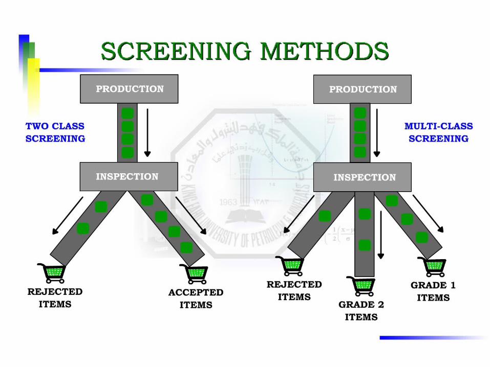
Targeting in Multi-Class Screening Under Error and Error Free Measurement Systems. Thesis Defense Presentation on. by ATIQ WALIULLAH SIDDIQUI. PRESENTATION OVERVIEW. Introduction Literature Review Objectives of the Thesis - PowerPoint PPT Presentation
Citation preview
Targeting in Multi-Class Screening Under Error and Error Free
Measurement Systems
Targeting in Multi-Class Screening Under Error and Error Free
Measurement Systems
Thesis Defense Presentationon
byATIQ WALIULLAH SIDDIQUI

PRESENTATION OVERVIEWPRESENTATION OVERVIEW
Introduction
Literature Review
Objectives of the Thesis
Multi-Class Screening Model Presented in Min Koo Lee and Joon Soon Jang (1997)
Model Extensions
Sensitivity Analysis
Model Comparisons
Conclusion
Introduction
Literature Review
Objectives of the Thesis
Multi-Class Screening Model Presented in Min Koo Lee and Joon Soon Jang (1997)
Model Extensions
Sensitivity Analysis
Model Comparisons
Conclusion
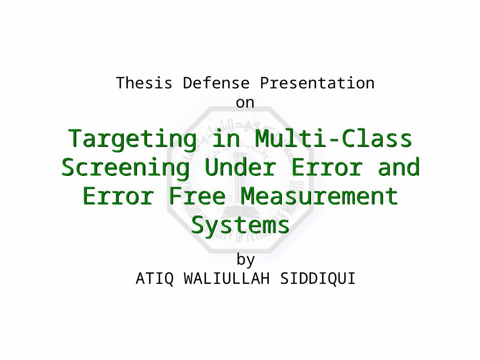
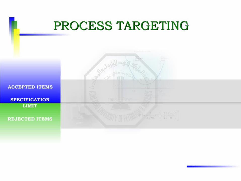
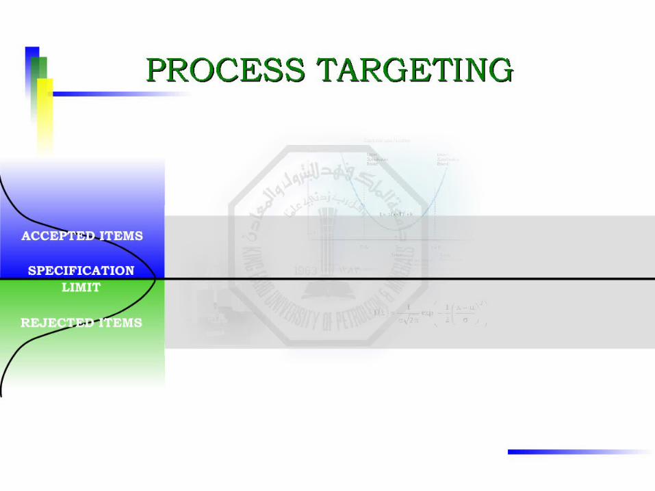
Fitness for Use
Conformance to Specifications
Penalties Associated with Product Deviations Off Target (within specification limits)
Fitness for Use
Conformance to Specifications
Penalties Associated with Product Deviations Off Target (within specification limits)
WHAT IS QUALITY?WHAT IS QUALITY?
LL UL Quality characteristic
LL UL Quality characteristic
CustomerTolerance
Cos
t of
re
pair
, $
Cos
t of
re
pair
, $
CustomerTolerance
Goal Post Syndrome Taguchi Loss Function Goal Post Syndrome Taguchi Loss Function
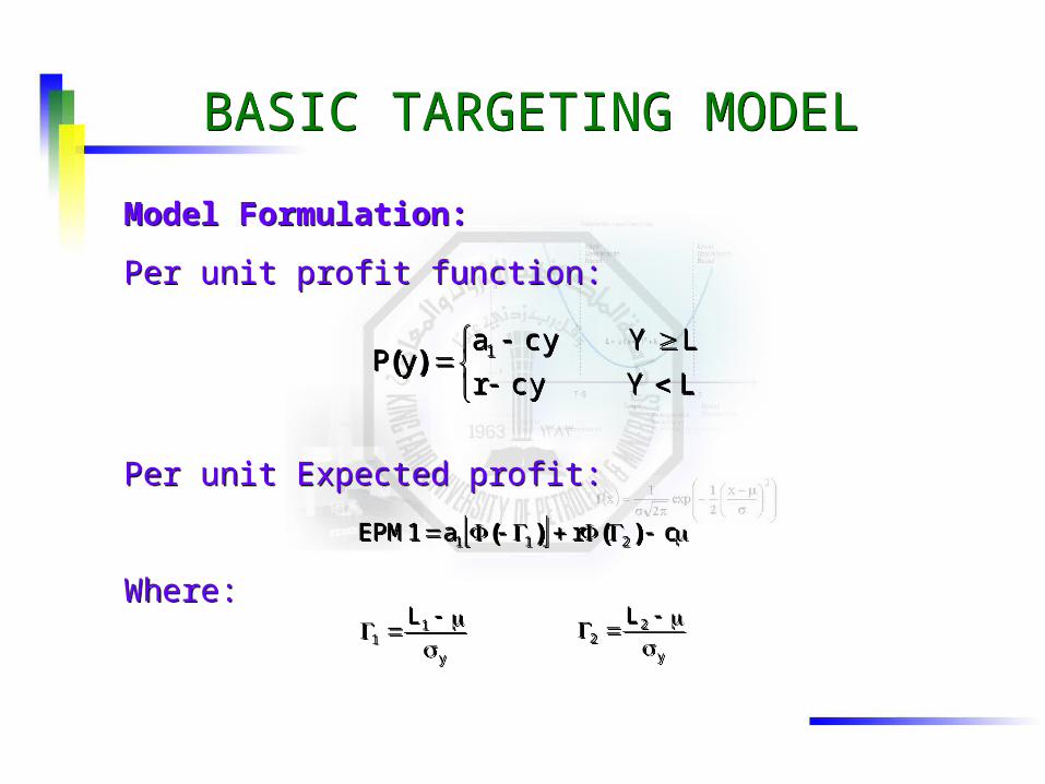
BASIC TARGETING MODELBASIC TARGETING MODEL
Model Formulation:
Per unit profit function:
Per unit Expected profit:
Where:
Model Formulation:
Per unit profit function:
Per unit Expected profit:
Where:
LYycr
LYycayP 1)(
LYycr
LYycayP 1)(
cra1EPM 211 )()( cra1EPM 211 )()(
y
11
L
y
11
L
y
22
L
y
22
L
LITERATURE REVIEWLITERATURE REVIEW
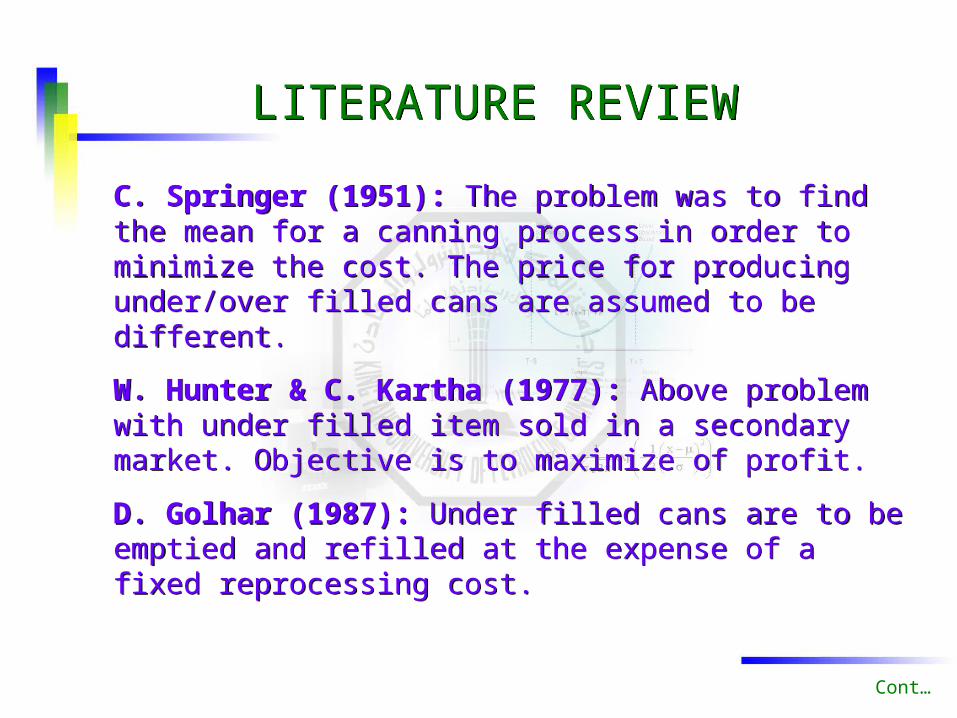
C. Springer (1951): The problem was to find the mean for a canning process in order to minimize the cost. The price for producing under/over filled cans are assumed to be different.
W. Hunter & C. Kartha (1977): Above problem with under filled item sold in a secondary market. Objective is to maximize of profit.
D. Golhar (1987): Under filled cans are to be emptied and refilled at the expense of a fixed reprocessing cost.
Cont…

LITERATURE REVIEWLITERATURE REVIEW
M. A. Rahim and P. K. Banerjee (1988): considered the process where the system has a linear drift (e.g., tool wear etc).
O. Carlsson (1989): determined, for the case of two variable characteristics, the optimum process mean under acceptance variable sampling.
R. Schmidt & P. Pfeifer (1989): investigated the effects on cost savings from variance reduction.
K. S. Al-Sultan (1994): addressed the problem of two machines in series.
Cont…
LITERATURE REVIEWLITERATURE REVIEW
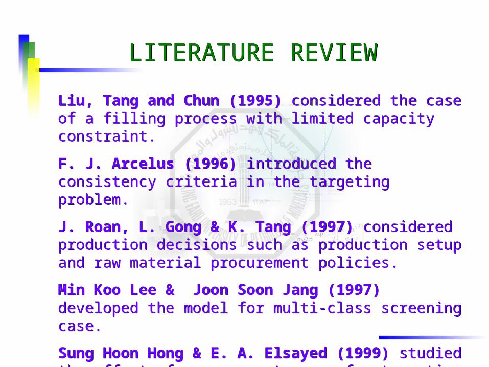
Liu, Tang and Chun (1995) considered the case of a filling process with limited capacity constraint.
F. J. Arcelus (1996) introduced the consistency criteria in the targeting problem.
J. Roan, L. Gong & K. Tang (1997) considered production decisions such as production setup and raw material procurement policies.
Min Koo Lee & Joon Soon Jang (1997) developed the model for multi-class screening case.
Sung Hoon Hong & E. A. Elsayed (1999) studied the effect of measurement error for targeting problem.
OBJECTIVES OF THE THESISOBJECTIVES OF THE THESIS
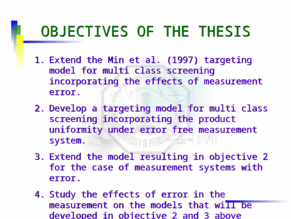
1. Extend the Min et al. (1997) targeting model for multi class screening incorporating the effects of measurement error.
2. Develop a targeting model for multi class screening incorporating the product uniformity under error free measurement system.
3. Extend the model resulting in objective 2 for the case of measurement systems with error.
4. Study the effects of error in the measurement on the models that will be developed in objective 2 and 3 above
MIN et al. (1997) MODEL MIN et al. (1997) MODEL
Model Assumptions:
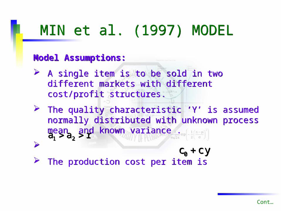
A single item is to be sold in two different markets with different cost/profit structures.
The quality characteristic ‘Y’ is assumed normally distributed with unknown process mean and known variance .
The production cost per item is
Model Assumptions:
A single item is to be sold in two different markets with different cost/profit structures.
The quality characteristic ‘Y’ is assumed normally distributed with unknown process mean and known variance .
The production cost per item is
raa 21 raa 21
Cont…
ycc0 ycc0
MIN et al. (1997) Model MIN et al. (1997) Model
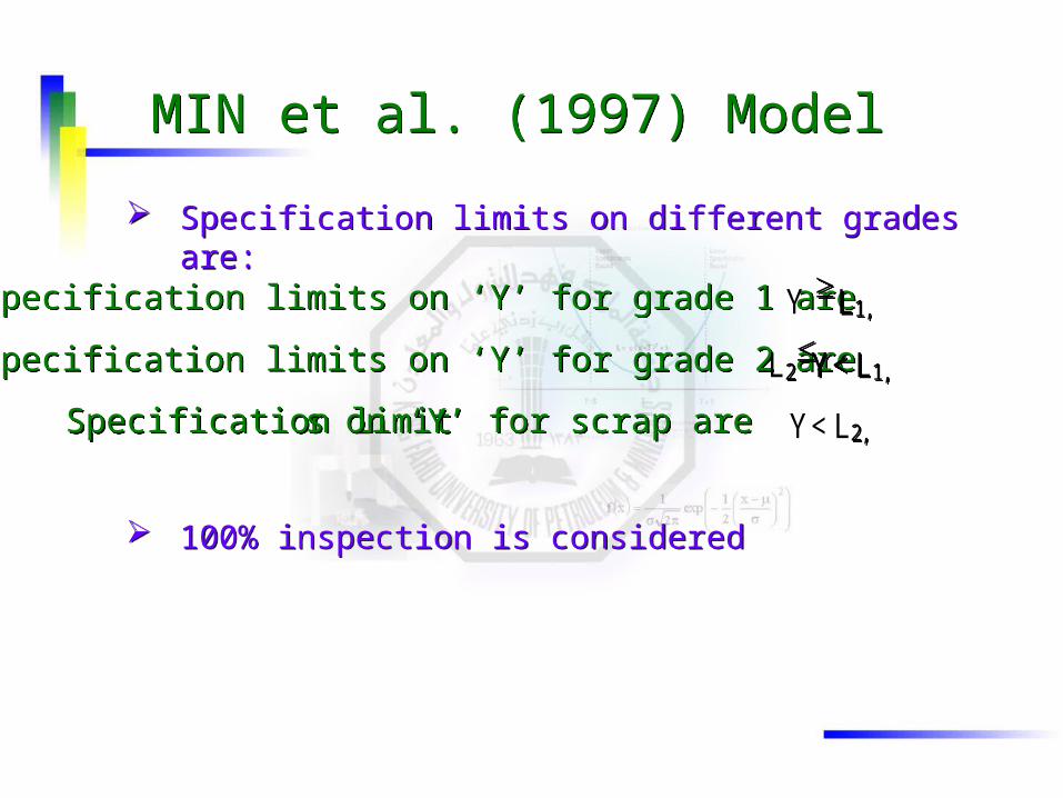
Specification limits on different grades are:
100% inspection is considered
Specification limits on different grades are:
100% inspection is considered
Specification limits on ‘Y’ for grade 1 areSpecification limits on ‘Y’ for grade 1 are
Specification limits on ‘Y’ for grade 2 areSpecification limits on ‘Y’ for grade 2 are
Specification limitSpecification limits on ‘Y’ for scrap ares on ‘Y’ for scrap are
Y L1,
L2Y< L1,
Y< L2,
Y L1,
L2Y< L1,
Y< L2,
MIN et al. (1997) Model MIN et al. (1997) Model
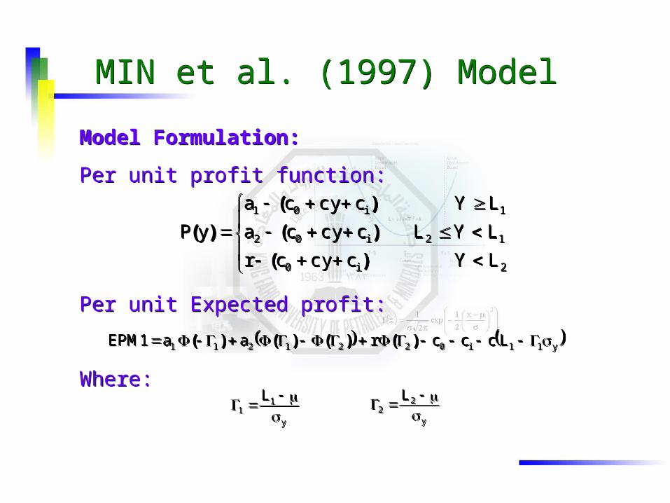
Model Formulation:
Per unit profit function:
Per unit Expected profit:
Where:
Model Formulation:
Per unit profit function:
Per unit Expected profit:
Where:
2i0
12i02
1i01
LYccycr
LYLccyca
LYccyca
yP
)(
)(
)(
)(
2i0
12i02
1i01
LYccycr
LYLccyca
LYccyca
yP
)(
)(
)(
)(
y11i0221211 Lcccraa1EPM )()()()( y11i0221211 Lcccraa1EPM )()()()(
y
11
L
y
11
L
y
22
L
y
22
L
OBJECTIVE 1:(Measurement error)OBJECTIVE 1:(Measurement error)
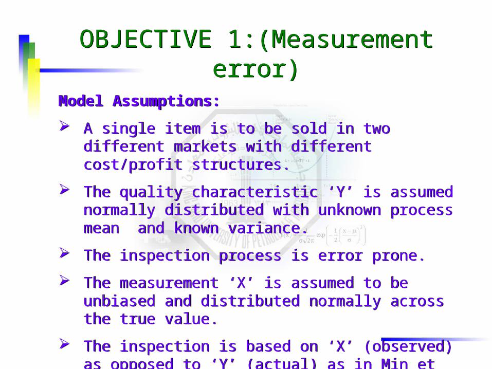
Model Assumptions:
A single item is to be sold in two different markets with different cost/profit structures.
The quality characteristic ‘Y’ is assumed normally distributed with unknown process mean and known variance.
The inspection process is error prone.
The measurement ‘X’ is assumed to be unbiased and distributed normally across the true value.
The inspection is based on ‘X’ (observed) as opposed to ‘Y’ (actual) as in Min et al. (1997).
OBJECTIVE 1:(Measurement error)OBJECTIVE 1:(Measurement error)
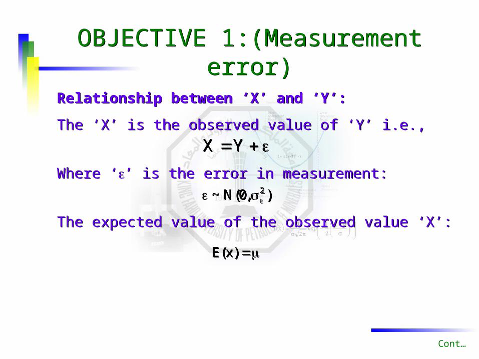
Relationship between ‘X’ and ‘Y’:
The ‘X’ is the observed value of ‘Y’ i.e.,
Where ‘’ is the error in measurement:
The expected value of the observed value ‘X’:
Relationship between ‘X’ and ‘Y’:
The ‘X’ is the observed value of ‘Y’ i.e.,
Where ‘’ is the error in measurement:
The expected value of the observed value ‘X’:
Cont…
Y X Y X
),0(N~ 2 ),0(N~ 2
)x(E )x(E
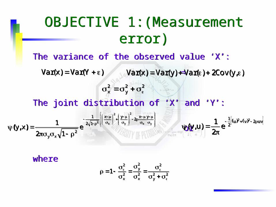
The variance of the observed value ‘X’:
The joint distribution of ‘X’ and ‘Y’:
or
where
The variance of the observed value ‘X’:
The joint distribution of ‘X’ and ‘Y’:
or
where
),y(Cov2)(Var)y(Var)x(Var ),y(Cov2)(Var)y(Var)x(Var
22y
2x 22
y2x
)Y(Var)x(Var )Y(Var)x(Var
OBJECTIVE 1:(Measurement error)OBJECTIVE 1:(Measurement error)
yx
2
y
2
x2
yx2
yx
12
1
2xy
e12
1xy ),(
yx
2
y
2
x2
yx2
yx
12
1
2xy
e12
1xy ),(
uv2vu2
1 22
e2
1)u,v(
uv2vu2
1 22
e2
1)u,v(
22y
2
2x
2y
2x
2
1
22y
2
2x
2y
2x
2
1
OBJECTIVE 1:(Measurement error)OBJECTIVE 1:(Measurement error)
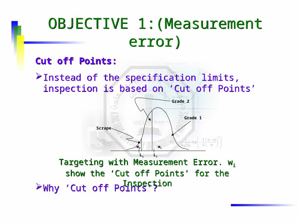
Cut off Points:
Instead of the specification limits, inspection is based on ‘Cut off Points’
Why ‘Cut off Points’?
Cut off Points:
Instead of the specification limits, inspection is based on ‘Cut off Points’
Why ‘Cut off Points’?
Grade 2
Grade 1
Scrape
L2 L1
w2 w1
Targeting with Measurement Error. wi show the ‘Cut off
Points’ for the Inspection
Targeting with Measurement Error. wi show the ‘Cut off Points’ for the Inspection
OBJECTIVE 1:(Measurement error)OBJECTIVE 1:(Measurement error)
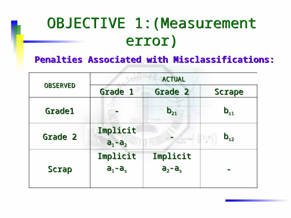
Penalties Associated with Misclassifications:Penalties Associated with Misclassifications:
OBSERVEDOBSERVEDACTUALACTUAL
Grade 1Grade 1 Grade 2Grade 2 ScrapeScrape
Grade1Grade1 -- bb2121 bbs1s1
Grade 2Grade 2ImplicitImplicit
aa11-a-a22
-- bbs2s2
ScrapScrap
ImplicitImplicit
aa11-a-ass
ImplicitImplicit
aa22-a-ass --
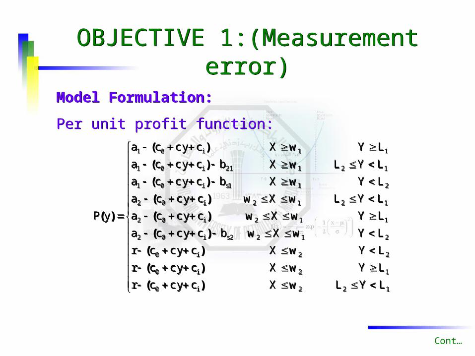
Model Formulation:
Per unit profit function:
Model Formulation:
Per unit profit function:
OBJECTIVE 1:(Measurement error)OBJECTIVE 1:(Measurement error)
122i0
12i0
22i0
2122si02
112i02
1212i02
211si01
12121i01
11i01
LYLwXccycr
LYwXccycr
LYwXccycr
LYwXwbccyca
LYwXwccyca
LYLwXwccyca
LYwXbccyca
LYLwXbccyca
LYwXccyca
yP
)(
)(
)(
)(
)(
)(
)(
)(
)(
)(
122i0
12i0
22i0
2122si02
112i02
1212i02
211si01
12121i01
11i01
LYLwXccycr
LYwXccycr
LYwXccycr
LYwXwbccyca
LYwXwccyca
LYLwXwccyca
LYwXbccyca
LYLwXbccyca
LYwXccyca
yP
)(
)(
)(
)(
)(
)(
)(
)(
)(
)(
Cont…
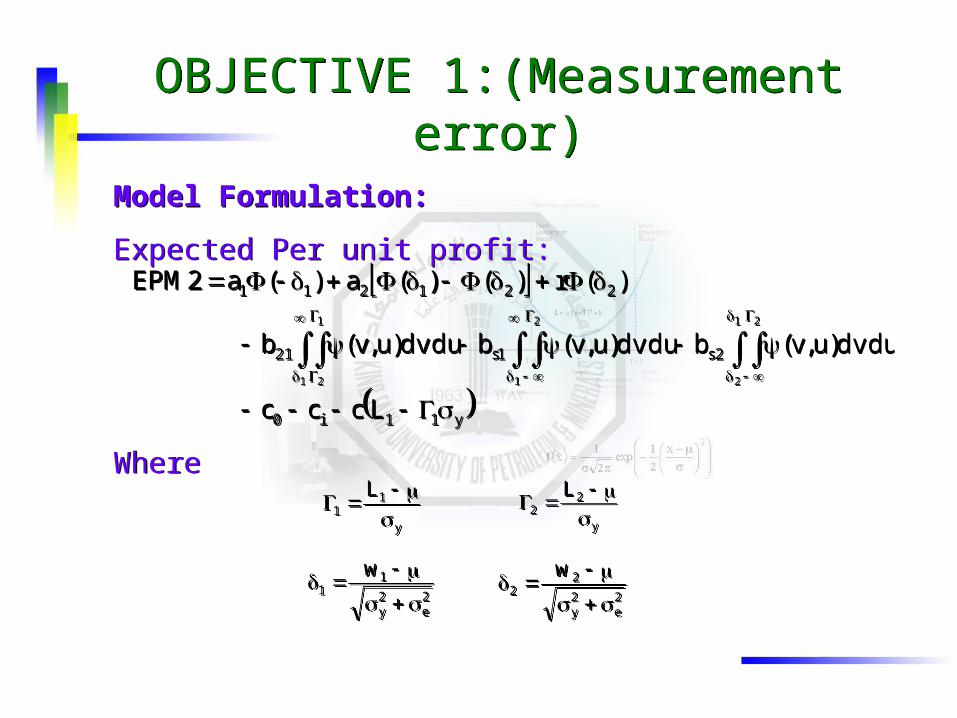
y11i0
2s1s21
221211
Lccc
dvdu)u,v(bdvdu)u,v(bdvdu)u,v(b
)(r)()(a)(a2EPM1
2
2
1
2
1
1
2
y11i0
2s1s21
221211
Lccc
dvdu)u,v(bdvdu)u,v(bdvdu)u,v(b
)(r)()(a)(a2EPM1
2
2
1
2
1
1
2
y
11
L
y
11
L
y
22
L
y
22
L
2e
2y
11
w
2e
2y
11
w
Model Formulation:
Expected Per unit profit:
Where
Model Formulation:
Expected Per unit profit:
Where
OBJECTIVE 1:(Measurement error)OBJECTIVE 1:(Measurement error)
2e
2y
22
w
2e
2y
22
w
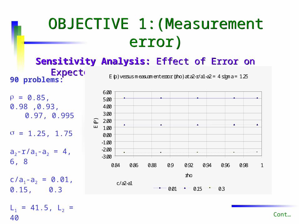
Sensitivity Analysis: Effect of Error on Expected Profit
Sensitivity Analysis: Effect of Error on Expected Profit
OBJECTIVE 1:(Measurement error)OBJECTIVE 1:(Measurement error)
E(p) versus measurment error (rho) at a2-r/ a1-a2 = 4 sigma = 1.25
-3.00-2.00-1.000.001.002.003.004.005.006.00
0.84 0.86 0.88 0.9 0.92 0.94 0.96 0.98 1
rho
E(P
)
0.01 0.15 0.3c/ a2-a1
90 problems:
= 0.85, 0.98 ,0.93,
0.97, 0.995
= 1.25, 1.75
a2-r/a1-a2 = 4, 6, 8
c/a1-a2 = 0.01, 0.15, 0.3
L1 = 41.5, L2 = 40
Cont…
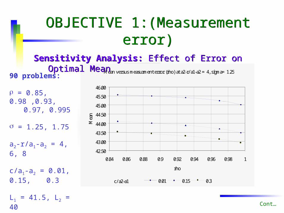
Mean versus measurment error (rho) at a2-r/ a1-a2 = 4, sigma= 1.25
42.50
43.00
43.50
44.00
44.50
45.00
45.50
46.00
0.84 0.86 0.88 0.9 0.92 0.94 0.96 0.98 1
rho
Mea
n
0.01 0.15 0.3c/ a2-a1
Sensitivity Analysis: Effect of Error on Optimal Mean
Sensitivity Analysis: Effect of Error on Optimal Mean
OBJECTIVE 1:(Measurement error)OBJECTIVE 1:(Measurement error)
90 problems:
= 0.85, 0.98 ,0.93,
0.97, 0.995
= 1.25, 1.75
a2-r/a1-a2 = 4, 6, 8
c/a1-a2 = 0.01, 0.15, 0.3
L1 = 41.5, L2 = 40
Cont…
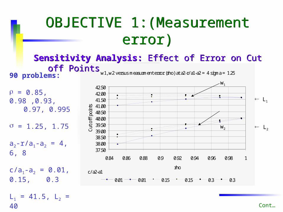
w1, w2 versus measurment error (rho) at a2-r/ a1-a2 = 4 sigma = 1.25
37.5038.0038.5039.0039.5040.0040.5041.0041.5042.0042.50
0.84 0.86 0.88 0.9 0.92 0.94 0.96 0.98 1
rho
Cut
off
poi
nts
0.01 0.01 0.15 0.15 0.3 0.3
c/ a2-a1
Sensitivity Analysis: Effect of Error on Cut off PointsSensitivity Analysis: Effect of Error on Cut off Points
OBJECTIVE 1:(Measurement error)OBJECTIVE 1:(Measurement error)
90 problems:
= 0.85, 0.98 ,0.93,
0.97, 0.995
= 1.25, 1.75
a2-r/a1-a2 = 4, 6, 8
c/a1-a2 = 0.01, 0.15, 0.3
L1 = 41.5, L2 = 40
Cont…
L1
L2
w1
w2
OBJECTIVE 2:(Uniformity Penalty)OBJECTIVE 2:(Uniformity Penalty)
Model Assumptions:
A single item is to be sold in two different markets with different cost/profit structures.
The quality characteristic ‘Y’ is assumed normally distributed with unknown process mean and known variance.
The inspection process is error free.
The inspection is based on ‘y’.
Model Assumptions:
A single item is to be sold in two different markets with different cost/profit structures.
The quality characteristic ‘Y’ is assumed normally distributed with unknown process mean and known variance.
The inspection process is error free.
The inspection is based on ‘y’.
Cont…
OBJECTIVE 2:(Uniformity Penalty)OBJECTIVE 2:(Uniformity Penalty)
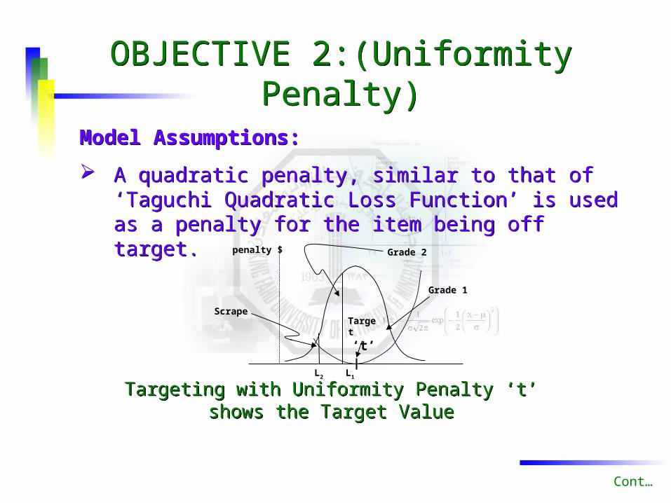
Model Assumptions:
A quadratic penalty, similar to that of ‘Taguchi Quadratic Loss Function’ is used as a penalty for the item being off target.
Model Assumptions:
A quadratic penalty, similar to that of ‘Taguchi Quadratic Loss Function’ is used as a penalty for the item being off target.
Cont…
Grade 2
Grade 1
Scrape
L2 L1
Targeting with Uniformity Penalty ‘t’ shows the Target Value
Targeting with Uniformity Penalty ‘t’ shows the Target Value
penalty $
Target
‘t’
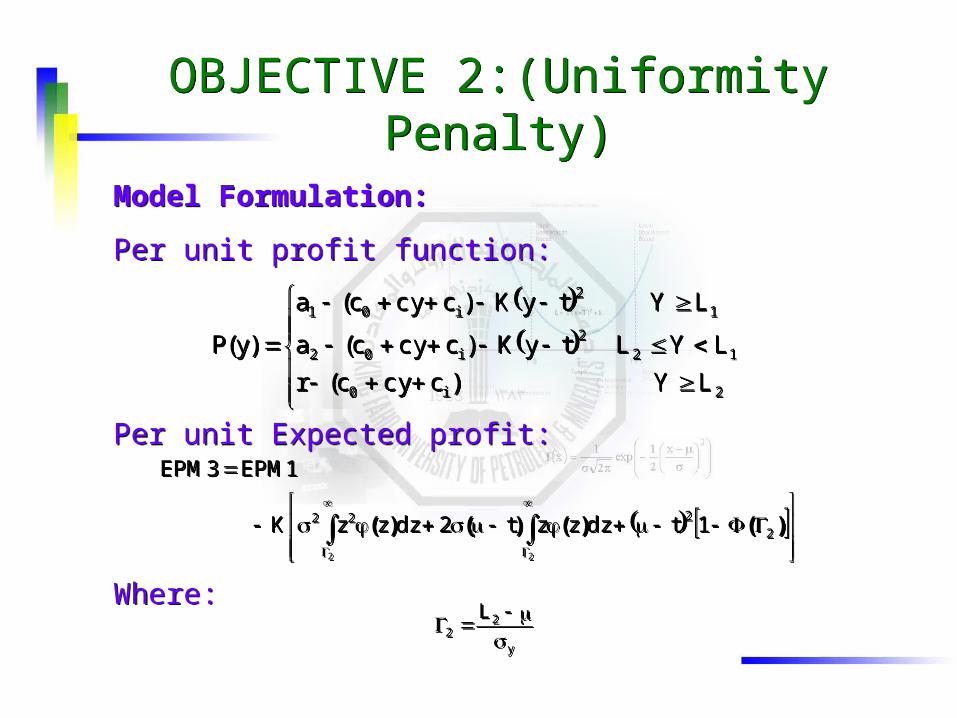
Model Formulation:
Per unit profit function:
Per unit Expected profit:
Where:
Model Formulation:
Per unit profit function:
Per unit Expected profit:
Where:
OBJECTIVE 2:(Uniformity Penalty)OBJECTIVE 2:(Uniformity Penalty)
2i0
122
i02
12
i01
LY)ccyc(r
LYLtyK)ccyc(a
LYtyK)ccyc(a
)y(P
2i0
122
i02
12
i01
LY)ccyc(r
LYLtyK)ccyc(a
LYtyK)ccyc(a
)y(P
)()()()( 2222 1tdzzzt2dzzzK
1EPM3EPM
22
)()()()( 2222 1tdzzzt2dzzzK
1EPM3EPM
22
y
22
L
y
22
L
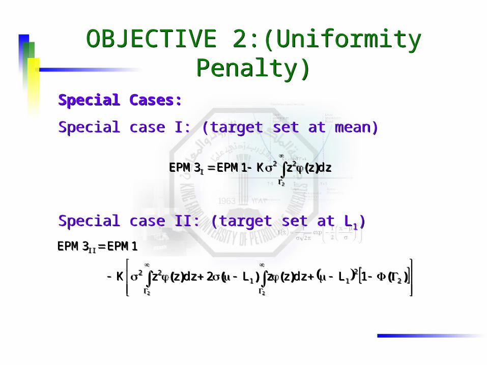
Special Cases:
Special case I: (target set at mean)
Special case II: (target set at L1)
Special Cases:
Special case I: (target set at mean)
Special case II: (target set at L1)
OBJECTIVE 2:(Uniformity Penalty)OBJECTIVE 2:(Uniformity Penalty)
2
dzzzK1EPM3EPM 22I )(
2
dzzzK1EPM3EPM 22I )(
)()()()( 22
1122
II
1LdzzzL2dzzzK
1EPM3EPM
22
)()()()( 22
1122
II
1LdzzzL2dzzzK
1EPM3EPM
22
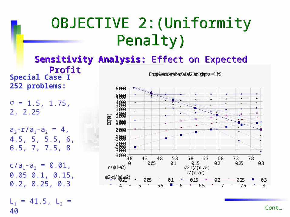
Sensitivity Analysis: Effect on Expected ProfitSensitivity Analysis: Effect on Expected Profit
OBJECTIVE 2:(Uniformity Penalty)OBJECTIVE 2:(Uniformity Penalty)
Special Case I252 problems:
= 1.5, 1.75, 2, 2.25
a2-r/a1-a2 = 4, 4.5, 5, 5.5, 6, 6.5, 7, 7.5, 8
c/a1-a2 = 0.01, 0.05 0.1, 0.15, 0.2, 0.25, 0.3
L1 = 41.5, L2 = 40
K = 0.05
Cont…
E(p) versus a2-r/ a1-a2 at sigma = 1.5
-3.000-2.000-1.0000.0001.0002.0003.0004.0005.0006.000
3.8 4.3 4.8 5.3 5.8 6.3 6.8 7.3 7.8
(a2-r)/ (a1-a2)
E(P
)
0.01 0.05 0.1 0.15 0.2 0.25 0.3
c/ (a1-a2)
E(p) versus c/ a1-a2 at sigma = 1.5
-3.000
-2.000
-1.000
0.000
1.000
2.000
3.000
4.000
5.000
0 0.05 0.1 0.15 0.2 0.25 0.3
c/ (a1-a2)
E(P
)
4 5 5.5 6 6.5 7 7.5 8
(a2-r)/ (a1-a2)
Optimal Mean versus a2-r/ a1-a2 at sigma = 1.5
42.500
43.000
43.500
44.000
44.500
45.000
45.500
46.000
4.5 5.0 5.5 6.0 6.5 7.0 7.5 8.0 8.5
(a2-r)/ (a1-a2)
Mu
0.01 0.05 0.1 0.15 0.2 0.25 0.3
c/ (a1-a2)
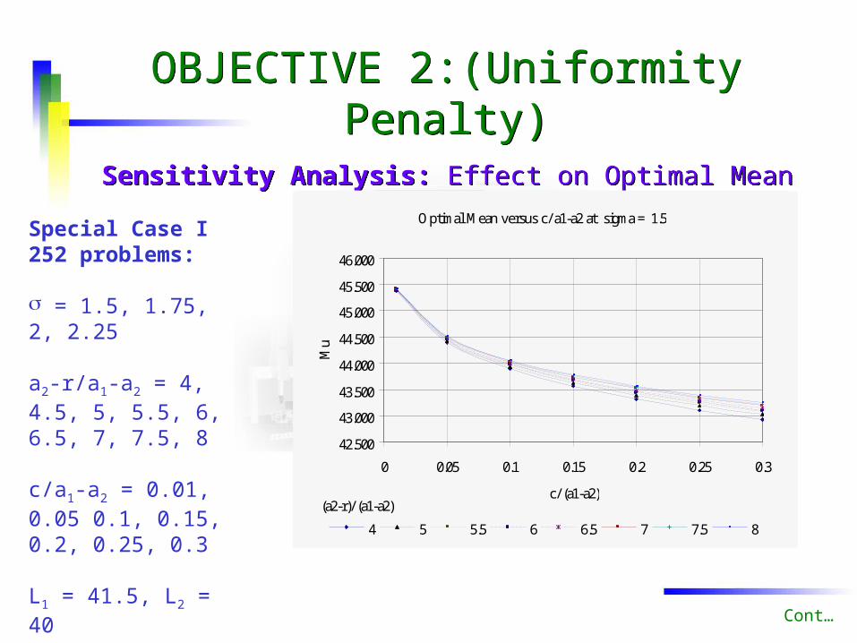
Sensitivity Analysis: Effect on Optimal MeanSensitivity Analysis: Effect on Optimal Mean
OBJECTIVE 2:(Uniformity Penalty)OBJECTIVE 2:(Uniformity Penalty)
Special Case I252 problems:
= 1.5, 1.75, 2, 2.25
a2-r/a1-a2 = 4, 4.5, 5, 5.5, 6, 6.5, 7, 7.5, 8
c/a1-a2 = 0.01, 0.05 0.1, 0.15, 0.2, 0.25, 0.3
L1 = 41.5, L2 = 40
K = 0.05
Cont…
Optimal Mean versus c/ a1-a2 at sigma = 1.5
42.500
43.000
43.500
44.000
44.500
45.000
45.500
46.000
0 0.05 0.1 0.15 0.2 0.25 0.3
c/ (a1-a2)
Mu
4 5 5.5 6 6.5 7 7.5 8
(a2-r)/ (a1-a2)
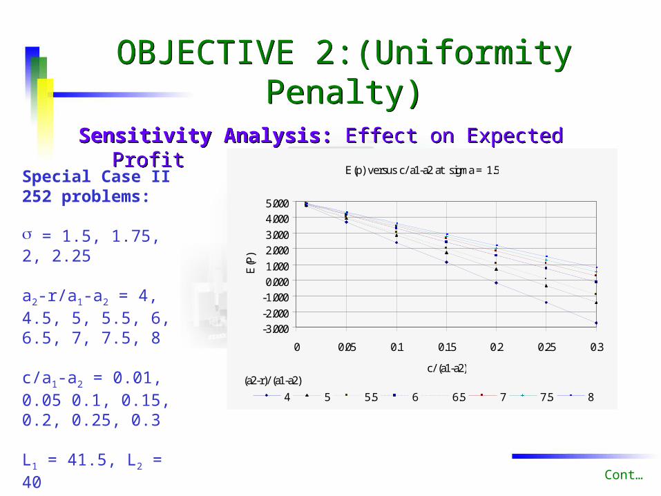
Sensitivity Analysis: Effect on Expected ProfitSensitivity Analysis: Effect on Expected Profit
OBJECTIVE 2:(Uniformity Penalty)OBJECTIVE 2:(Uniformity Penalty)
Special Case II252 problems:
= 1.5, 1.75, 2, 2.25
a2-r/a1-a2 = 4, 4.5, 5, 5.5, 6, 6.5, 7, 7.5, 8
c/a1-a2 = 0.01, 0.05 0.1, 0.15, 0.2, 0.25, 0.3
L1 = 41.5, L2 = 40
K = 0.05
Cont…
E(p) versus a2-r/ a1-a2 at sigma = 1.5
-3.000
-1.000
1.000
3.000
5.000
3.8 4.3 4.8 5.3 5.8 6.3 6.8 7.3 7.8
(a2-r)/ (a1-a2)
E(P
)
0.01 0.05 0.1 0.15 0.2 0.25 0.3
c/ (a1-a2)
E(p) versus c/ a1-a2 at sigma = 1.5
-3.000-2.000-1.0000.0001.0002.0003.0004.0005.000
0 0.05 0.1 0.15 0.2 0.25 0.3
c/ (a1-a2)
E(P
)
4 5 5.5 6 6.5 7 7.5 8
(a2-r)/ (a1-a2)
Optimal Mean versus a2-r/ a1-a2 at sigma = 1.5
42.400
42.500
42.600
42.700
42.800
42.900
43.000
43.100
43.200
4.5 5.0 5.5 6.0 6.5 7.0 7.5 8.0 8.5
(a2-r)/ (a1-a2)
Mea
n
0.01 0.05 0.1 0.15 0.2 0.25 0.3
c/ (a1-a2)
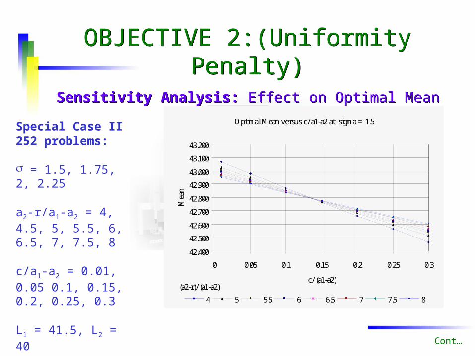
Sensitivity Analysis: Effect on Optimal MeanSensitivity Analysis: Effect on Optimal Mean
OBJECTIVE 2:(Uniformity Penalty)OBJECTIVE 2:(Uniformity Penalty)
Special Case II252 problems:
= 1.5, 1.75, 2, 2.25
a2-r/a1-a2 = 4, 4.5, 5, 5.5, 6, 6.5, 7, 7.5, 8
c/a1-a2 = 0.01, 0.05 0.1, 0.15, 0.2, 0.25, 0.3
L1 = 41.5, L2 = 40
K = 0.05
Cont…
Optimal Mean versus c/ a1-a2 at sigma = 1.5
42.400
42.500
42.600
42.700
42.800
42.900
43.000
43.100
43.200
0 0.05 0.1 0.15 0.2 0.25 0.3
c/ (a1-a2)
Mea
n
4 5 5.5 6 6.5 7 7.5 8
(a2-r)/ (a1-a2)
OBJECTIVE 3:(Integrated Model)OBJECTIVE 3:(Integrated Model)
Cont…
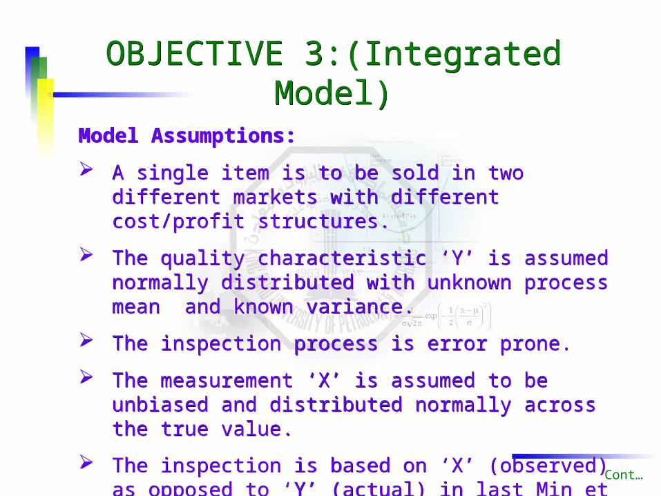
Model Assumptions:
A single item is to be sold in two different markets with different cost/profit structures.
The quality characteristic ‘Y’ is assumed normally distributed with unknown process mean and known variance.
The inspection process is error prone.
The measurement ‘X’ is assumed to be unbiased and distributed normally across the true value.
The inspection is based on ‘X’ (observed) as opposed to ‘Y’ (actual) in last Min et al. (1997).
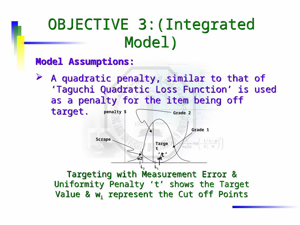
Model Assumptions:
A quadratic penalty, similar to that of ‘Taguchi Quadratic Loss Function’ is used as a penalty for the item being off target.
Model Assumptions:
A quadratic penalty, similar to that of ‘Taguchi Quadratic Loss Function’ is used as a penalty for the item being off target.
Grade 2
Grade 1
Scrape
L2 L1
Targeting with Measurement Error & Uniformity Penalty ‘t’ shows the Target Value & wi represent the Cut off Points
Targeting with Measurement Error & Uniformity Penalty ‘t’ shows the Target Value & wi represent the Cut off Points
penalty $
Target
‘t’w2 w1
OBJECTIVE 3:(Integrated Model)OBJECTIVE 3:(Integrated Model)
OBJECTIVE 3:(Integrated Model)OBJECTIVE 3:(Integrated Model)
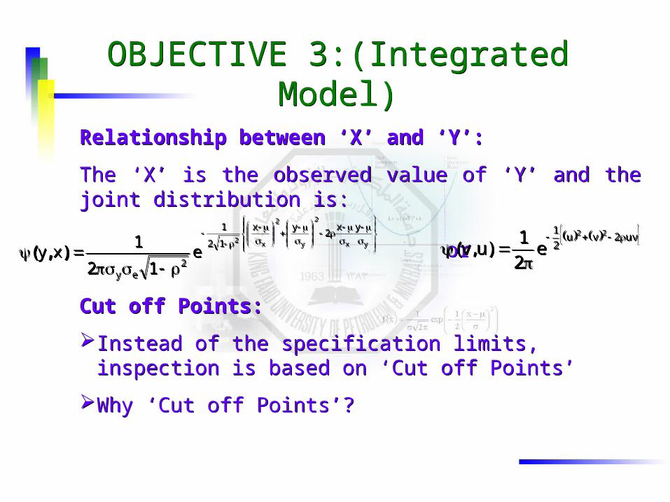
Relationship between ‘X’ and ‘Y’:
The ‘X’ is the observed value of ‘Y’ and the joint distribution is:
or
Relationship between ‘X’ and ‘Y’:
The ‘X’ is the observed value of ‘Y’ and the joint distribution is:
or
yx
2
y
2
x2
yx2
yx
12
1
2ey
e12
1xy ),(
yx
2
y
2
x2
yx2
yx
12
1
2ey
e12
1xy ),(
uv2vu2
1 22
e2
1)u,v(
uv2vu2
1 22
e2
1)u,v(
Cut off Points:
Instead of the specification limits, inspection is based on ‘Cut off Points’
Why ‘Cut off Points’?
Cut off Points:
Instead of the specification limits, inspection is based on ‘Cut off Points’
Why ‘Cut off Points’?
OBJECTIVE 3:(Integrated Model)OBJECTIVE 3:(Integrated Model)
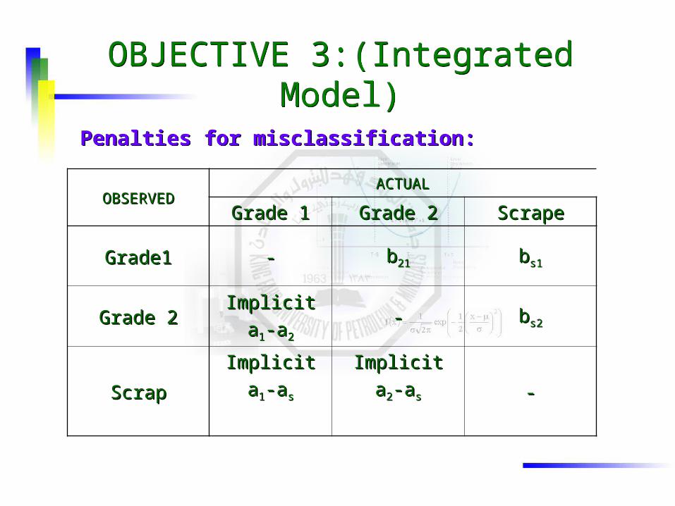
Penalties for misclassification:Penalties for misclassification:
OBSERVEDOBSERVEDACTUALACTUAL
Grade 1Grade 1 Grade 2Grade 2 ScrapeScrape
Grade1Grade1 -- bb2121 bbs1s1
Grade 2Grade 2ImplicitImplicit
aa11-a-a22
-- bbs2s2
ScrapScrap
ImplicitImplicit
aa11-a-ass
ImplicitImplicit
aa22-a-ass --
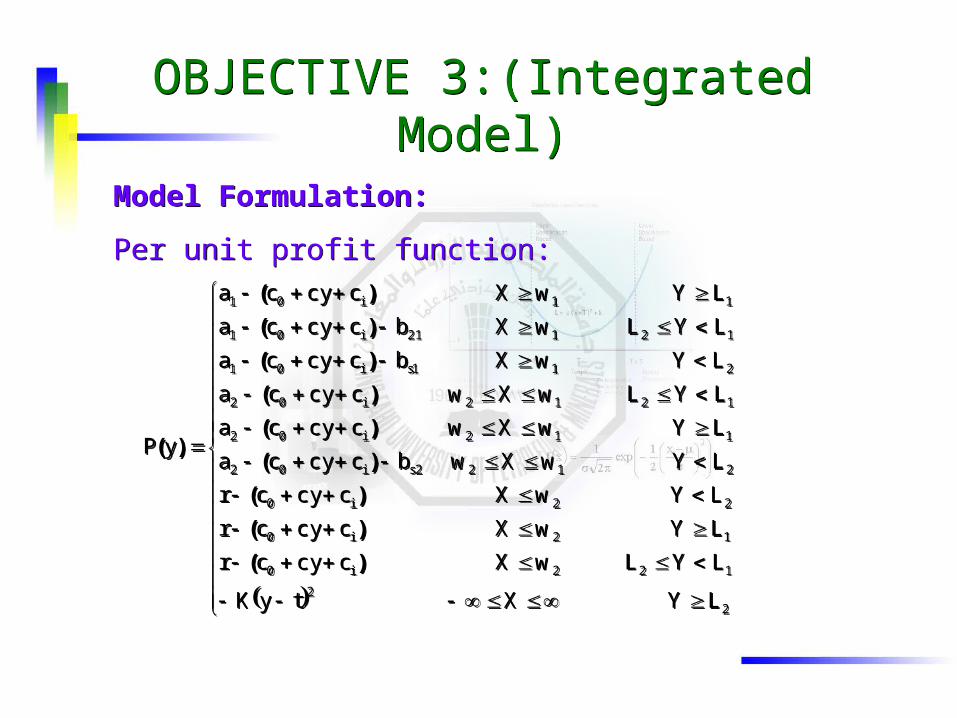
OBJECTIVE 3:(Integrated Model)OBJECTIVE 3:(Integrated Model)
Model Formulation:
Per unit profit function:
Model Formulation:
Per unit profit function:
22
122i0
12i0
22i0
2122si02
112i02
1212i02
211si01
12121i01
11i01
LYXtyK
LYLwXccycr
LYwXccycr
LYwXccycr
LYwXwbccyca
LYwXwccyca
LYLwXwccyca
LYwXbccyca
LYLwXbccyca
LYwXccyca
yP
)(
)(
)(
)(
)(
)(
)(
)(
)(
)(
22
122i0
12i0
22i0
2122si02
112i02
1212i02
211si01
12121i01
11i01
LYXtyK
LYLwXccycr
LYwXccycr
LYwXccycr
LYwXwbccyca
LYwXwccyca
LYLwXwccyca
LYwXbccyca
LYLwXbccyca
LYwXccyca
yP
)(
)(
)(
)(
)(
)(
)(
)(
)(
)(
OBJECTIVE 3:(Integrated Model)OBJECTIVE 3:(Integrated Model)
y
22
L
y
22
L
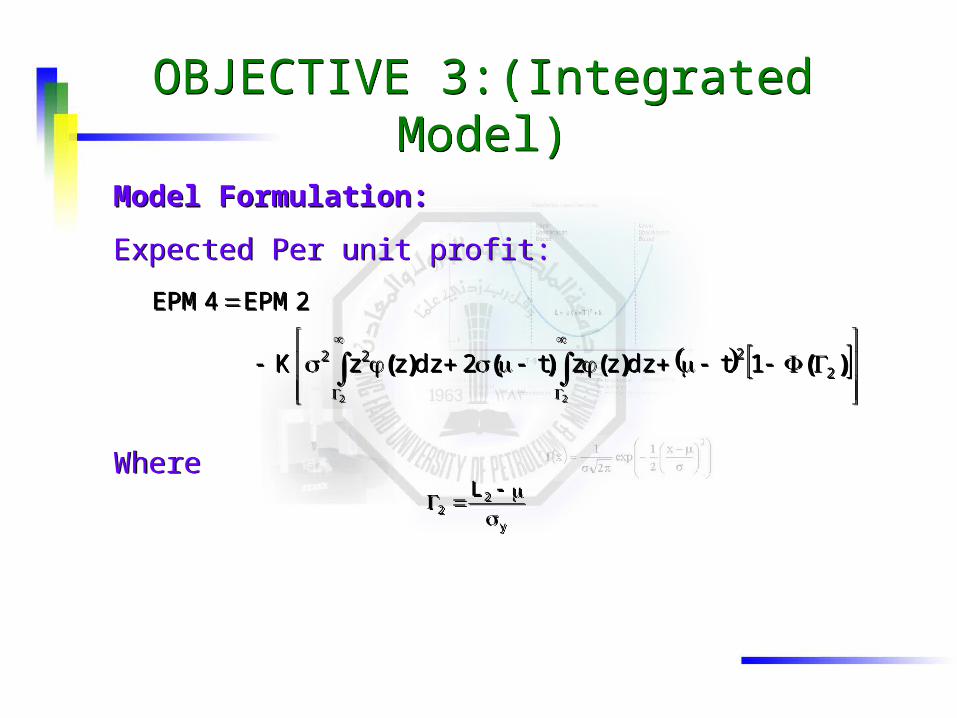
Model Formulation:
Expected Per unit profit:
Where
Model Formulation:
Expected Per unit profit:
Where
)()()()( 2222 1tdzzzt2dzzzK
2EPM4EPM
22
)()()()( 2222 1tdzzzt2dzzzK
2EPM4EPM
22
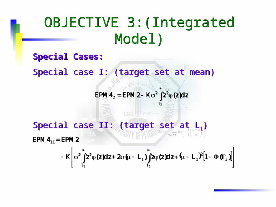
OBJECTIVE 3:(Integrated Model)OBJECTIVE 3:(Integrated Model)
Special Cases:
Special case I: (target set at mean)
Special case II: (target set at L1)
Special Cases:
Special case I: (target set at mean)
Special case II: (target set at L1)
2
dzzzK2EPM4EPM 22I )(
2
dzzzK2EPM4EPM 22I )(
)()()()( 22
1122
II
1LdzzzL2dzzzK
2EPM4EPM
22
)()()()( 22
1122
II
1LdzzzL2dzzzK
2EPM4EPM
22
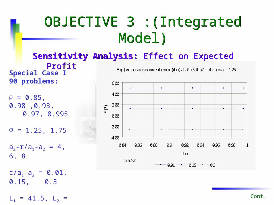
Sensitivity Analysis: Effect on Expected ProfitSensitivity Analysis: Effect on Expected Profit
OBJECTIVE 3 :(Integrated Model)OBJECTIVE 3 :(Integrated Model)
Cont…
E(p) versus measurment error (rho) at a2-r/ a1-a2 = 4, sigma = 1.25
-4.00
-2.00
0.00
2.00
4.00
6.00
0.84 0.86 0.88 0.9 0.92 0.94 0.96 0.98 1
rho
E(P
)
0.01 0.15 0.3c/ a2-a1
Special Case I90 problems:
= 0.85, 0.98 ,0.93,
0.97, 0.995
= 1.25, 1.75
a2-r/a1-a2 = 4, 6, 8
c/a1-a2 = 0.01, 0.15, 0.3
L1 = 41.5, L2 = 40
K = 0.05
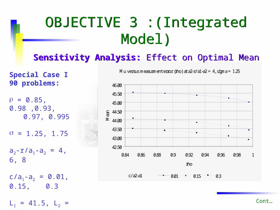
Mu versus measurment error (rho) at a2-r/ a1-a2 = 4, sigma = 1.25
42.50
43.00
43.50
44.00
44.50
45.00
45.50
46.00
0.84 0.86 0.88 0.9 0.92 0.94 0.96 0.98 1
rho
Mea
n
0.01 0.15 0.3c/ a2-a1
Sensitivity Analysis: Effect on Optimal MeanSensitivity Analysis: Effect on Optimal Mean
Cont…
Special Case I90 problems:
= 0.85, 0.98 ,0.93,
0.97, 0.995
= 1.25, 1.75
a2-r/a1-a2 = 4, 6, 8
c/a1-a2 = 0.01, 0.15, 0.3
L1 = 41.5, L2 = 40
K = 0.05
OBJECTIVE 3 :(Integrated Model)OBJECTIVE 3 :(Integrated Model)
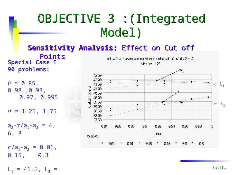
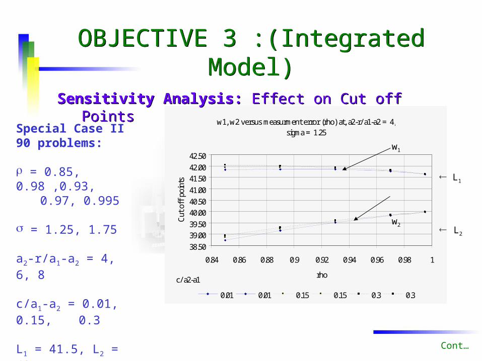
Sensitivity Analysis: Effect on Cut off PointsSensitivity Analysis: Effect on Cut off Points
Cont…
Special Case I90 problems:
= 0.85, 0.98 ,0.93,
0.97, 0.995
= 1.25, 1.75
a2-r/a1-a2 = 4, 6, 8
c/a1-a2 = 0.01, 0.15, 0.3
L1 = 41.5, L2 = 40
K = 0.05
w1, w2 versus measurment error (rho) at a2-r/ a1-a2 = 4, sigma = 1.25
37.5038.0038.5039.0039.5040.0040.5041.0041.5042.0042.50
0.84 0.86 0.88 0.9 0.92 0.94 0.96 0.98 1
rho
Cut
off
poi
nts
0.01 0.01 0.15 0.15 0.3 0.3
c/ a2-a1
OBJECTIVE 3 :(Integrated Model)OBJECTIVE 3 :(Integrated Model)
w1
w2
L1
L2
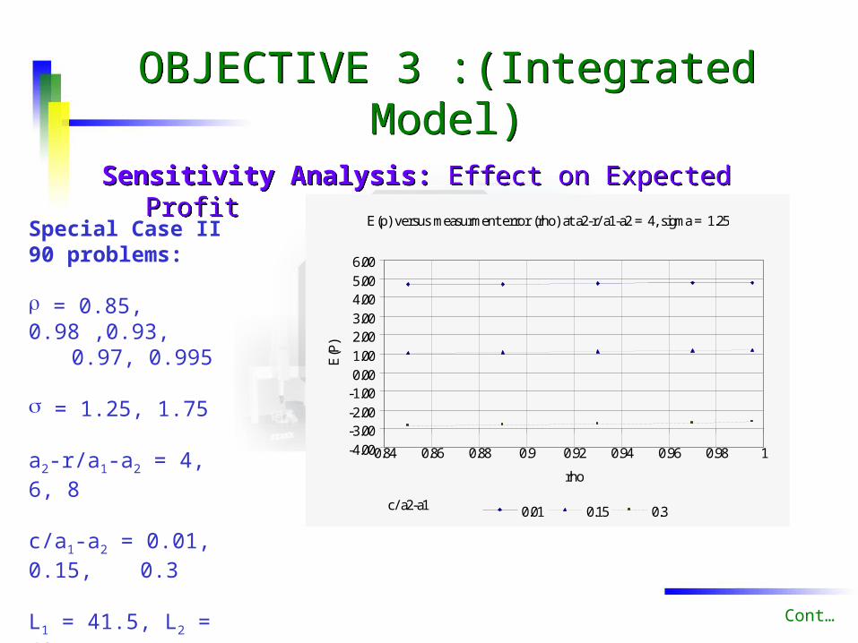
Sensitivity Analysis: Effect on Expected ProfitSensitivity Analysis: Effect on Expected Profit
Cont…
Special Case II90 problems:
= 0.85, 0.98 ,0.93,
0.97, 0.995
= 1.25, 1.75
a2-r/a1-a2 = 4, 6, 8
c/a1-a2 = 0.01, 0.15, 0.3
L1 = 41.5, L2 = 40
K = 0.05
E(p) versus measurment error (rho) at a2-r/ a1-a2 = 4, sigma = 1.25
-4.00-3.00-2.00-1.000.001.002.003.004.005.006.00
0.84 0.86 0.88 0.9 0.92 0.94 0.96 0.98 1
rho
E(P
)
0.01 0.15 0.3c/ a2-a1
OBJECTIVE 3 :(Integrated Model)OBJECTIVE 3 :(Integrated Model)
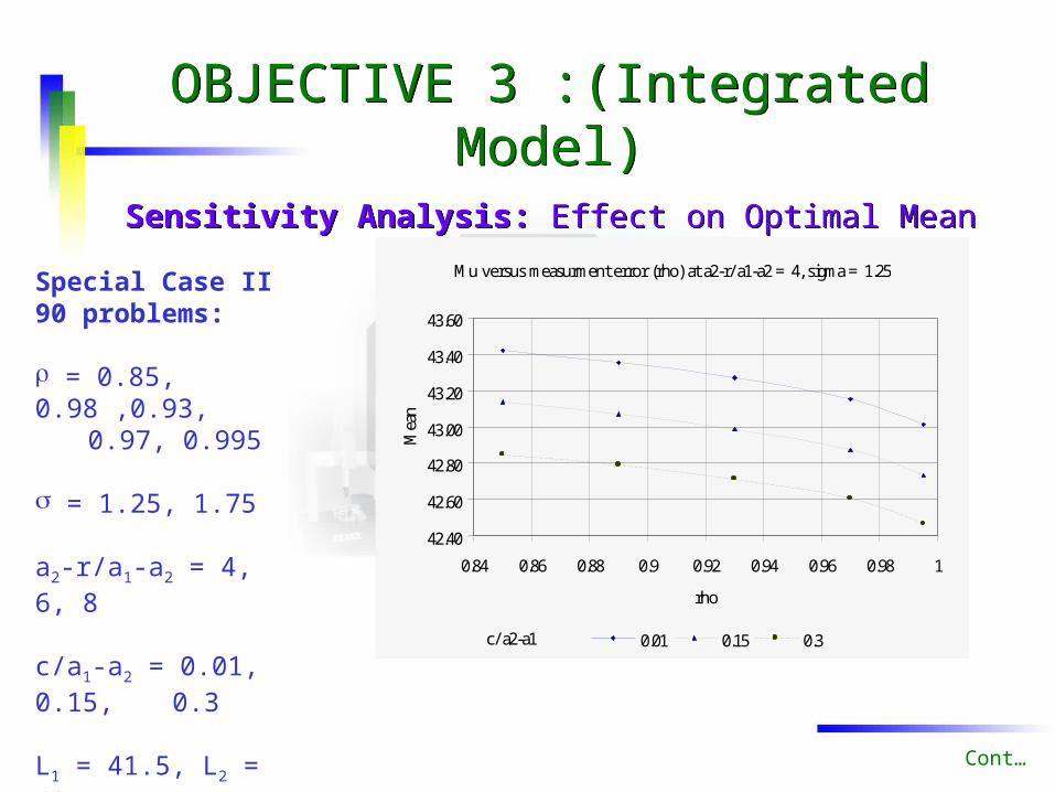
Sensitivity Analysis: Effect on Optimal MeanSensitivity Analysis: Effect on Optimal Mean
Special Case II90 problems:
= 0.85, 0.98 ,0.93,
0.97, 0.995
= 1.25, 1.75
a2-r/a1-a2 = 4, 6, 8
c/a1-a2 = 0.01, 0.15, 0.3
L1 = 41.5, L2 = 40
K = 0.05
Cont…
Mu versus measurment error (rho) at a2-r/ a1-a2 = 4, sigma = 1.25
42.40
42.60
42.80
43.00
43.20
43.40
43.60
0.84 0.86 0.88 0.9 0.92 0.94 0.96 0.98 1
rho
Mea
n
0.01 0.15 0.3c/ a2-a1
OBJECTIVE 3 :(Integrated Model)OBJECTIVE 3 :(Integrated Model)
w1, w2 versus measurment error (rho) at, a2-r/ a1-a2 = 4, sigma = 1.25
38.5039.0039.5040.0040.5041.0041.5042.0042.50
0.84 0.86 0.88 0.9 0.92 0.94 0.96 0.98 1
rho
Cut
off
poi
nts
0.01 0.01 0.15 0.15 0.3 0.3
c/ a2-a1
Sensitivity Analysis: Effect on Cut off PointsSensitivity Analysis: Effect on Cut off Points
Cont…
Special Case II90 problems:
= 0.85, 0.98 ,0.93,
0.97, 0.995
= 1.25, 1.75
a2-r/a1-a2 = 4, 6, 8
c/a1-a2 = 0.01, 0.15, 0.3
L1 = 41.5, L2 = 40
K = 0.05
OBJECTIVE 3 :(Integrated Model)OBJECTIVE 3 :(Integrated Model)
w1
w2
L1
L2
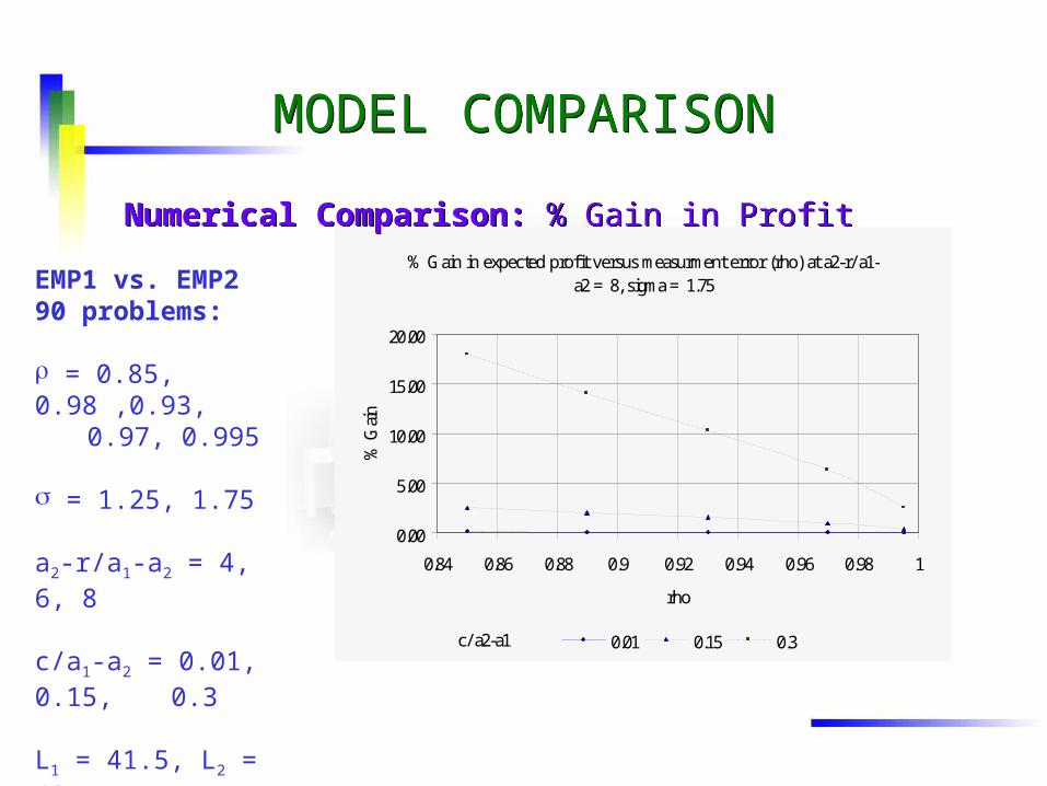
% Gain in expected profit versus measurment error (rho) at a2-r/ a1-a2 = 8, sigma = 1.75
0.00
5.00
10.00
15.00
20.00
0.84 0.86 0.88 0.9 0.92 0.94 0.96 0.98 1
rho
% G
ain
0.01 0.15 0.3c/ a2-a1
MODEL COMPARISONMODEL COMPARISON
EMP1 vs. EMP290 problems:
= 0.85, 0.98 ,0.93,
0.97, 0.995
= 1.25, 1.75
a2-r/a1-a2 = 4, 6, 8
c/a1-a2 = 0.01, 0.15, 0.3
L1 = 41.5, L2 = 40
Numerical Comparison: % Gain in ProfitNumerical Comparison: % Gain in Profit
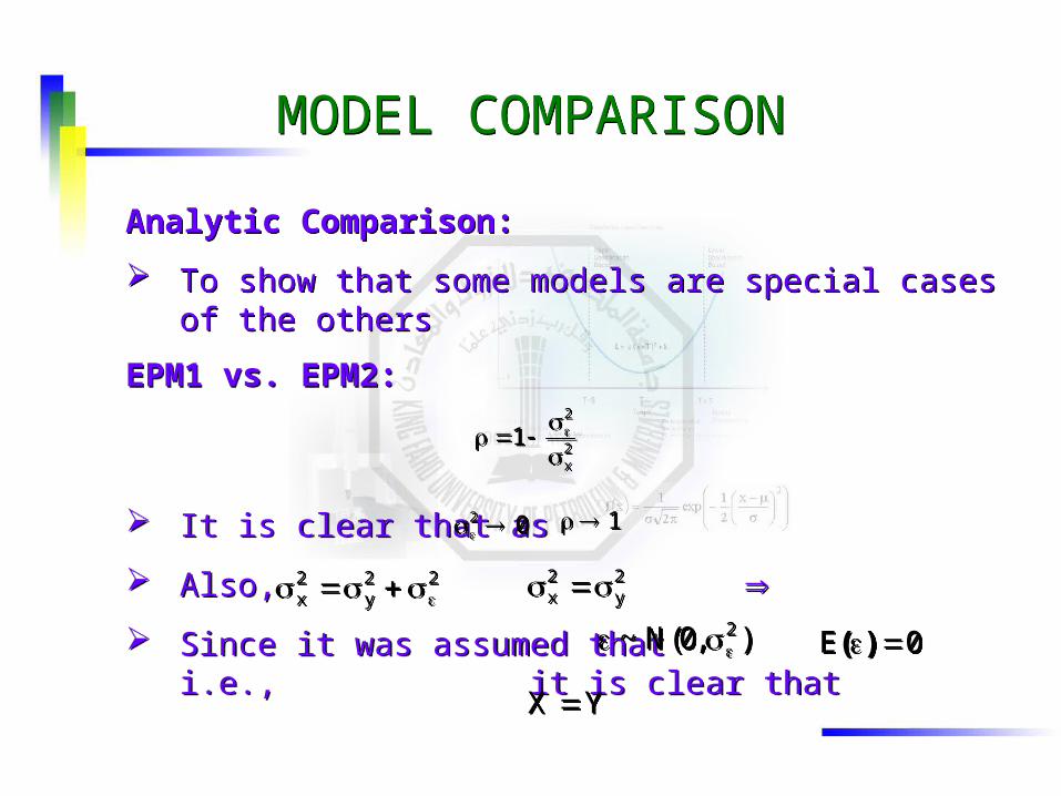
MODEL COMPARISONMODEL COMPARISON
Analytic Comparison:
To show that some models are special cases of the others
Analytic Comparison:
To show that some models are special cases of the others
EPM1 vs. EPM2:
It is clear that as
Also,
Since it was assumed that i.e., it is clear that
EPM1 vs. EPM2:
It is clear that as
Also,
Since it was assumed that i.e., it is clear that
2x
2
1
2x
2
1
02 02 1 1
22y
2x 22
y2x 2
y2x 2
y2x
),0(N~ 2 ),0(N~ 2 0E )( 0E )(
YX YX
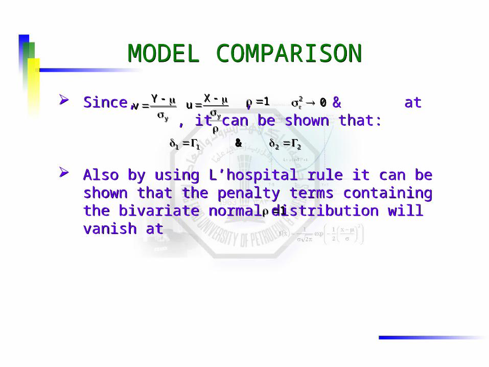
MODEL COMPARISONMODEL COMPARISON
Since, , & at , it can be shown that:
Also by using L’hospital rule it can be shown that the penalty terms containing the bivariate normal distribution will vanish at
Since, , & at , it can be shown that:
Also by using L’hospital rule it can be shown that the penalty terms containing the bivariate normal distribution will vanish at
y
Yv
y
Yv
y
Xu
y
Xu 02 02 1 1
2211 & 2211 &
1 1
MODEL COMPARISONMODEL COMPARISON
y11i0
2s1s21
221211
Lccc
dvduuvbdvduuvbdvduuvb
raa2EPM1
2
2
1
2
1
1
2
),(),(),(
)()()()(
y11i0
2s1s21
221211
Lccc
dvduuvbdvduuvbdvduuvb
raa2EPM1
2
2
1
2
1
1
2
),(),(),(
)()()()(
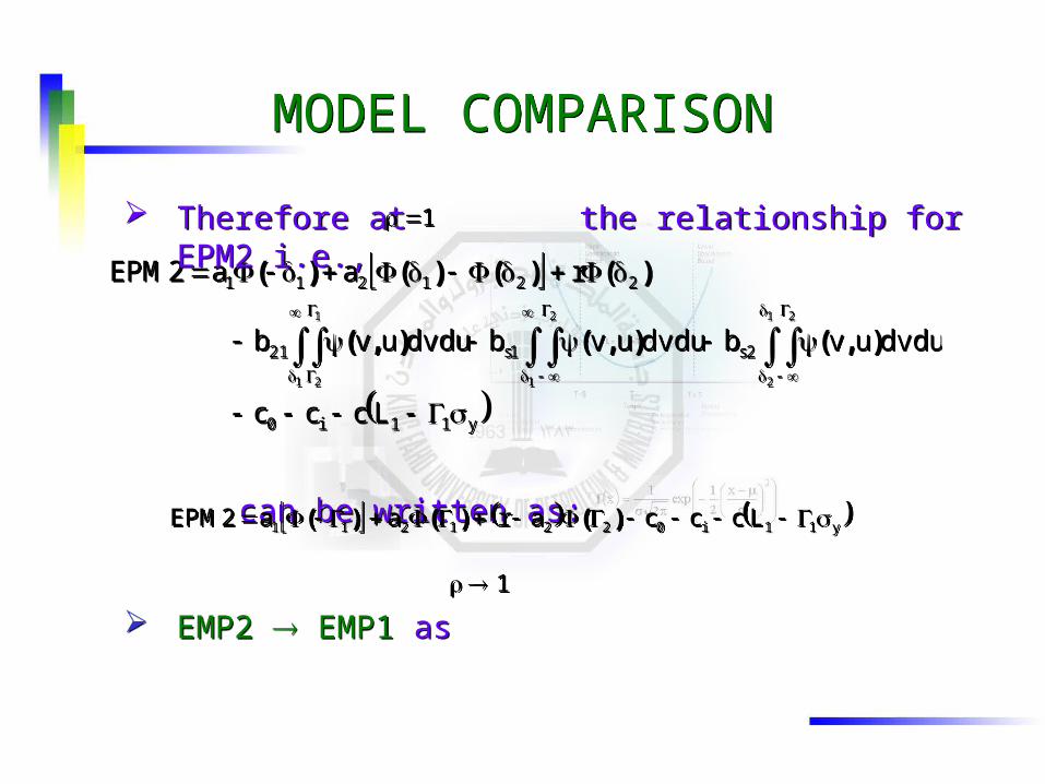
Therefore at the relationship for EPM2 i.e.,
can be written as:
EMP2 EMP1 as
Therefore at the relationship for EPM2 i.e.,
can be written as:
EMP2 EMP1 as
1 1
y11i0221211 Lcccaraa2EPM )()()( y11i0221211 Lcccaraa2EPM )()()(
1 1
MODEL COMPARISONMODEL COMPARISON
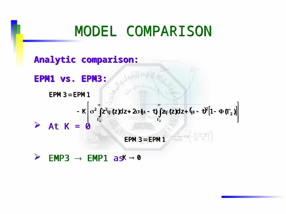
Analytic comparison:Analytic comparison:
EPM1 vs. EPM3:
At K = 0
EMP3 EMP1 as
EPM1 vs. EPM3:
At K = 0
EMP3 EMP1 as
)()()()( 2222 1tdzzzt2dzzzK
1EPM3EPM
22
)()()()( 2222 1tdzzzt2dzzzK
1EPM3EPM
22
1EPM3EPM 1EPM3EPM
0K 0K
MODEL COMPARISONMODEL COMPARISON
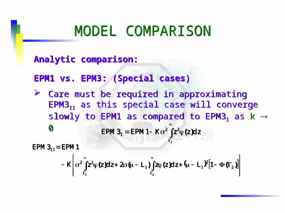
Analytic comparison:Analytic comparison:
EPM1 vs. EPM3: (Special cases)
Care must be required in approximating EPM3II as this special case will converge slowly to EPM1 as compared to EPM3I as k 0
EPM1 vs. EPM3: (Special cases)
Care must be required in approximating EPM3II as this special case will converge slowly to EPM1 as compared to EPM3I as k 0
2
dzzzK1EPM3EPM 22I )(
2
dzzzK1EPM3EPM 22I )(
)()()()( 22
1122
II
1LdzzzL2dzzzK
1EPM3EPM
22
)()()()( 22
1122
II
1LdzzzL2dzzzK
1EPM3EPM
22
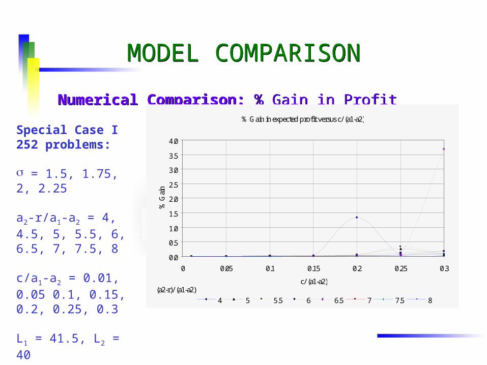
MODEL COMPARISONMODEL COMPARISON
Numerical Comparison: % Gain in ProfitNumerical Comparison: % Gain in Profit% Gain in expected profit versus c/ (a1-a2)
0.0
0.5
1.0
1.5
2.0
2.5
3.0
3.5
4.0
0 0.05 0.1 0.15 0.2 0.25 0.3
c/ (a1-a2)
% G
ain
4 5 5.5 6 6.5 7 7.5 8
(a2-r)/ (a1-a2)
Special Case I252 problems:
= 1.5, 1.75, 2, 2.25
a2-r/a1-a2 = 4, 4.5, 5, 5.5, 6, 6.5, 7, 7.5, 8
c/a1-a2 = 0.01, 0.05 0.1, 0.15, 0.2, 0.25, 0.3
L1 = 41.5, L2 = 40
K = 0.05
MODEL COMPARISONMODEL COMPARISON
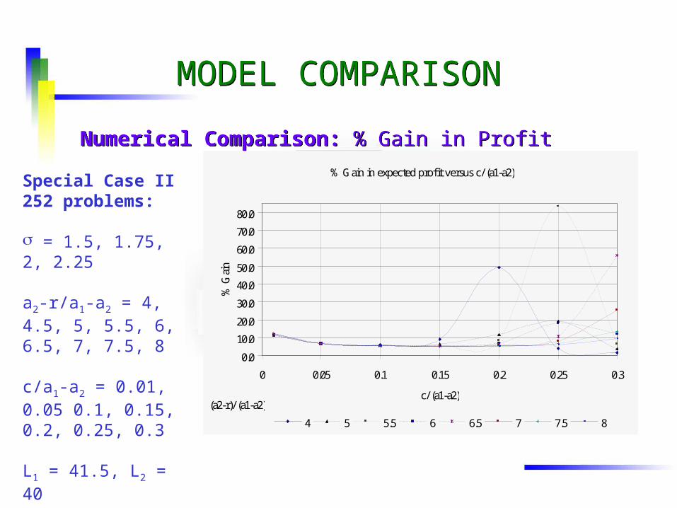
Numerical Comparison: % Gain in ProfitNumerical Comparison: % Gain in Profit
Special Case II252 problems:
= 1.5, 1.75, 2, 2.25
a2-r/a1-a2 = 4, 4.5, 5, 5.5, 6, 6.5, 7, 7.5, 8
c/a1-a2 = 0.01, 0.05 0.1, 0.15, 0.2, 0.25, 0.3
L1 = 41.5, L2 = 40
K = 0.05
% Gain in expected profit versus c/ (a1-a2)
0.0
10.0
20.0
30.0
40.0
50.0
60.0
70.0
80.0
0 0.05 0.1 0.15 0.2 0.25 0.3
c/ (a1-a2)
% G
ain
4 5 5.5 6 6.5 7 7.5 8
(a2-r)/ (a1-a2)
MODEL COMPARISONMODEL COMPARISON
Analytic comparison:Analytic comparison:
EPM2 vs. EPM4:
At K = 0
EMP4 EMP2 as
EPM2 vs. EPM4:
At K = 0
EMP4 EMP2 as
2EPM4EPM 2EPM4EPM
0K 0K
MODEL COMPARISONMODEL COMPARISON
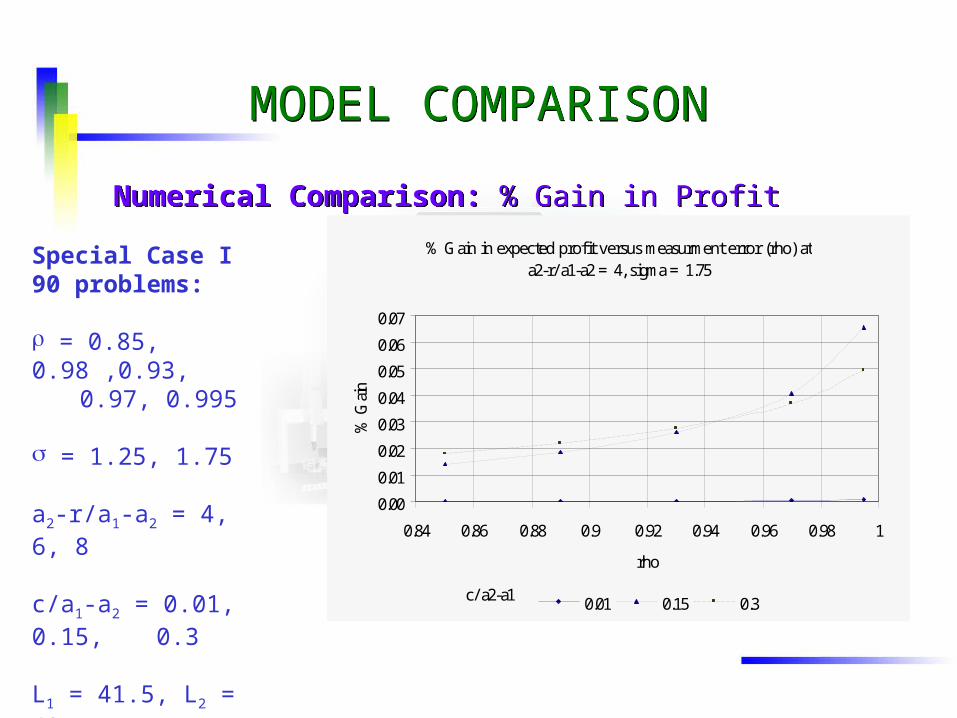
Numerical Comparison: % Gain in ProfitNumerical Comparison: % Gain in Profit
Special Case I90 problems:
= 0.85, 0.98 ,0.93,
0.97, 0.995
= 1.25, 1.75
a2-r/a1-a2 = 4, 6, 8
c/a1-a2 = 0.01, 0.15, 0.3
L1 = 41.5, L2 = 40
K = 0.05
% Gain in expected profit versus measurment error (rho) at a2-r/ a1-a2 = 4, sigma = 1.75
0.00
0.01
0.02
0.03
0.04
0.05
0.06
0.07
0.84 0.86 0.88 0.9 0.92 0.94 0.96 0.98 1
rho
% G
ain
0.01 0.15 0.3c/ a2-a1

MODEL COMPARISONMODEL COMPARISON
Numerical Comparison: % Gain in ProfitNumerical Comparison: % Gain in Profit
Special Case II90 problems:
= 0.85, 0.98 ,0.93,
0.97, 0.995
= 1.25, 1.75
a2-r/a1-a2 = 4, 6, 8
c/a1-a2 = 0.01, 0.15, 0.3
L1 = 41.5, L2 = 40
K = 0.05
% Gain in expected profit versus measurment error (rho) at a2-r/ a1-a2 = 4, sigma = 1.75
0.05.0
10.015.020.025.030.035.040.0
0.84 0.86 0.88 0.9 0.92 0.94 0.96 0.98 1
rho
% G
ain
0.01 0.15 0.3c/ a2-a1
MODEL COMPARISONMODEL COMPARISON
Analytic comparison:Analytic comparison:
EPM4 vs. EPM3:
The uniformity penalty term in both the models are same. The only difference is of EMP2 in EPM4 as compared to EPM1 in EPM3
As it is already shown that EMP2 EMP1 as error goes to zero
Therefore the proof of EMP4 EMP3 as is trivial
EPM4 vs. EPM3:
The uniformity penalty term in both the models are same. The only difference is of EMP2 in EPM4 as compared to EPM1 in EPM3
As it is already shown that EMP2 EMP1 as error goes to zero
Therefore the proof of EMP4 EMP3 as is trivial
1 1
MODEL COMPARISONMODEL COMPARISON
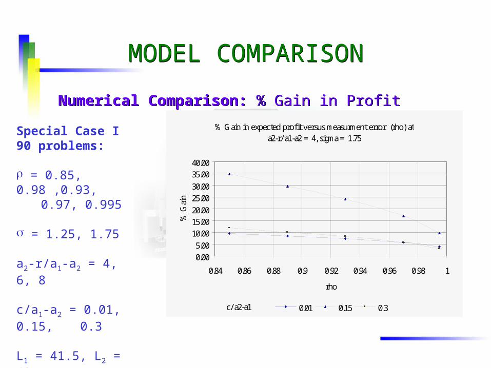
Numerical Comparison: % Gain in ProfitNumerical Comparison: % Gain in Profit
Special Case I90 problems:
= 0.85, 0.98 ,0.93,
0.97, 0.995
= 1.25, 1.75
a2-r/a1-a2 = 4, 6, 8
c/a1-a2 = 0.01, 0.15, 0.3
L1 = 41.5, L2 = 40
K = 0.05
% Gain in expected profit versus measurment error (rho) at a2-r/ a1-a2 = 4, sigma = 1.75
0.005.00
10.0015.0020.0025.0030.0035.0040.00
0.84 0.86 0.88 0.9 0.92 0.94 0.96 0.98 1
rho
% G
ain
0.01 0.15 0.3c/ a2-a1
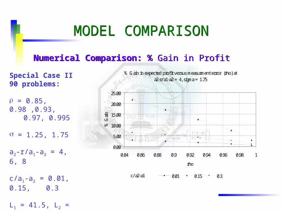
MODEL COMPARISONMODEL COMPARISON
Numerical Comparison: % Gain in ProfitNumerical Comparison: % Gain in Profit
Special Case II90 problems:
= 0.85, 0.98 ,0.93,
0.97, 0.995
= 1.25, 1.75
a2-r/a1-a2 = 4, 6, 8
c/a1-a2 = 0.01, 0.15, 0.3
L1 = 41.5, L2 = 40
K = 0.05
% Gain in expected profit versus measurment error (rho) at a2-r/ a1-a2 = 4, sigma = 1.75
0.00
5.00
10.00
15.00
20.00
25.00
0.84 0.86 0.88 0.9 0.92 0.94 0.96 0.98 1
rho
% G
ain
0.01 0.15 0.3c/ a2-a1
CONCLUSIONSCONCLUSIONS
Three models were developed for various multi-class screening targeting problems
EPM2 (measurement error) performed well in minimizing the effect of error
This effect is relatively less at higher cost
The effect of cost is more pronounced as compared to selling prices
In EPM3, the effect of uniformity penalty, if the target is set other than Mean, is high even at very low values of K
CONCLUSIONSCONCLUSIONS
In EPM4 the effect of measurement error and uniformity penalty were integrated
The numerical comparison show significant gain in profit if more realistic model is used
Gain in the case of error is higher with the higher error
Gains are also significant, even at low values of K, if the Target is set farther from the mean

FUTURE RESEARCHFUTURE RESEARCH
Process Targeting is an active area for research.
It has the potential to be appreciably beneficial for the industry.
The few of the direction from this work are
Process Targeting is an active area for research.
It has the potential to be appreciably beneficial for the industry.
The few of the direction from this work are
Generalization for the n-class screening situation
Other sampling plans, instead of 100% inspection
Processes with drift
Machines in series
Integration of other production decisions
Generalization for the n-class screening situation
Other sampling plans, instead of 100% inspection
Processes with drift
Machines in series
Integration of other production decisions

THANK YOUTHANK YOU