Target-matrix Construction Algorithms

Patrick Knupp∗

Applied Mathematics & Applications Department,Sandia National Laboratories,

M/S 1318, P.O. Box 5800,Albuquerque, NM 87185-1318

(pknupp@sandia.gov)

30 September 2009

Abstract

A gap in the series of reports describing the Target-matrix paradigm for mesh optimiza-

tion is filled by describing a method for automatic construction of Target-matrices, so

that diverse applications such as shape improvement, geometric-adaptivity, solution-

adaptivity, mesh alignment, and anisotropic smoothing can be served while using only

a limited set of local quality metrics. The method makes use of the Jacobian matrices

at sample points in the initial mesh. A QR-factorization is applied to the Jacobian

matrix to isolate different initial mesh properties such as Size, Shape, and Orientation.

To construct a Target-matrix, each factor can be retained if the goal is to preserve the

property of the initial mesh, or it can be replaced by a new factor based on application

or other data if the goal is to improve the initial property. By this method, one can

rapidly implement custom-made mesh optimization algorithms in response to requests

from application groups desiring improved meshes in order to perform more accurate

and efficient simulations. An example from a Cubit application is given.

1 Introduction

This work is part of a series of papers [1]-[5] which are devoted to a description and anal-ysis of the Target-matrix paradigm (TMP) for mesh optimization. Previous papers in theseries have focused on the overall TMP formulation, objective functions, and investigationsinto local quality metrics (including barriers, convexity, derivatives, and other essentialproperties). The present paper fills a critical gap, namely a description of methods forautomatically constructing the Target-matrices. Target-matrices are required in all TMPoptimization problems.

Targets play a critical role in the paradigm because they are the means by which applicationsdescribe the particular mesh optimization problem they wish to solve. There are, perhaps,a dozen distinct high-level applications of mesh optimization including shape improvement,geometric-adaptivity, solution-adaptivity, mesh alignment, and anisotropic smoothing. InTMP, each application requires a different set of Target-matrices that, along with the lo-cal quality metric, precisely define the goal of the optimization. For example, to adapt amesh to the local discretization error requires a different set of target-matrices than theproblem of optimizing a mesh to increase minimum edge-length. TMP moves the burden inmesh optimization from designing or selecting good local quality metrics to the automatic

∗This document is SAND 2009-XXX. This work was funded by the Department of Energy’s Mathematics,Information, and Computational Science Program (SC-31) and was performed at Sandia National Labora-tories. Sandia is a multiprogram laboratory operated by Sandia Corporation, a Lockheed Martin Company,for the U.S. Department of Energy under contract DE-ACO4-94AL85000. This work was performed byan employee of the U.S. Government or under U.S. Government contract. The U.S. Government retains anonexclusive, royalty-free license to publish or reproduce the published form of this contribution, or allowothers to do so, for U.S. Government purposes.

1

construction of target matrices derived from application goals. As with other methods, con-struction of targets remains somewhat of an art, but in TMP is made more tractable for tworeasons. First, the targets are based on the Jacobian matrix of the desired optimal meshand thus have a simple geometric interpretation. Second, the target construction methodmakes use of the initial mesh (the one to be optimized). The initial mesh is nearly alwaysavailable, and, in most other optimization methods, is ignored, even though it often containsvaluable information. Before describing methods for target construction, a brief review ofthe TMP follows.

First, one defines a set of local mappings from points Ξ in the master element(s) to pointsX(Ξ) in each of the elements in the mesh that is to be optimized (the latter is called theactive mesh). These mappings are most commonly those from linear finite elements, butcan be more general if needed. If the active mesh consists of only one element type, then themappings can all have the same form, e.g., the linear map from a square to a quadrilateral.If the active mesh contains more than one element type (e.g., tetradehra and triangularwedges) then more than one mapping form is required. Although the form of the mappingmay be the same from one element to another, the exact mapping on each element can differbecause the mapping depends on the coordinates of the vertices which define the particularelement. Non-linear mappings are also allowed, for example, in the case of high-order finiteelements.

In addition to the mappings, TMP requires that a set of sample points within the masterelement(s) be selected. Let the sample points within the master element be denoted by{Ξk}, k = 0, 1, . . . ,K − 1. The corresponding points in the active mesh are {Xk} whereXk = X(Ξk). Typically, the sample points are located at the corners of the master elementif the element is linear, otherwise they may also be located at mid-edges, mid-faces, and/ormid-elements. TMP thus requires that, in the formulation stage of the optimization, onedefine a set of mappings and sample points over all the elements of the mesh. This is not asdaunting as it sounds because the mappings are usually of the same form for each element inthe mesh (unless it contains more than one element type) and thus there is only one masterelement that is used for every element in the active mesh. The sample points are usuallylocated at the corners of the master element if the mapping is linear.

The mappings are required to be differentiable so that their Jacobian matrix ∂X/∂Ξ existsat the sample points. For short-hand, we denote this Jacobian matrix by the symbol A,which refers to the Jacobian of the map from the master element to an element in the active

mesh. The Jacobian matrix depends upon the vertex coordinates within each element andthus varies from one element to the next; this dependence is suppressed in the notationused above. Furthermore, the Jacobian matrix varies from point to point within the masterelement, as a function of Ξ. We denote by Ak the Jacobian matrix evaluated at samplepoint k; thus Ak = A(Ξk).

There is yet another requirement in TMP, namely the creation of a set of Target-matrices;the requirement is more difficult to achieve, but gives TMP considerable power and flexibil-ity. For every sample point k in the mesh, the target paradigm requires two matrices: theJacobian matrix Ak derived from the active mesh and the Target (or reference-Jacobian)-matrix Wk. The set matrices {Ak} is readily computed from the active mesh, while theset {Wk} must be constructed prior to the optimization. This construction is the subjectof the present paper. The purpose of the Target-matrices is to quantitatively describe theoptimal mesh Jacobians on the set of sample points. Since every sample point can havea different Target-matrix, this information is very detailed and difficult to determine fromscratch. Fortunately, there are mitigating factors (to be described later) which can be takenadvantage of to find suitable target sets.

For clarity, the sample point indices are often suppressed in much of the remainder of thispresentation. Let A and W at some sample point be defined. Because the construction oftargets is under our control, we can assume that, for every target, det(W ) 6= 0 and thus W−1

exists. The weighted Jacobian matrix T , defined by T = AW−1, is heavily used in TMPbecause, if the target matrix W has units of length (as does A), then T is non-dimensionaland provides a convenient scaling of A.

Before getting into the details of how the Targets are created, let us complete the descriptionof TMP. Let Md be the set of d × d matrices with real numbers as elements. In meshoptimization the matrices A, W , and T are either 2 × 2 or 3 × 3, reflecting the dimensionof the elements in the mesh.1. A local quality metric µ, which is a function from Md tothe non-negative numbers, is chosen from a set of quality metrics given in previous TMPpapers; for example, the Size+Shape+Orientation metric µ(T ) = |T −I|2 is frequently used,as are Shape and Size+Shape metrics. Note that both A and T depend on the coordinatesof the vertices within each element. An objective function, typically of the form

F =1

N

∑

e

∑

k

µ(T ek )

where k is the sample point index within an element, e is the element index, and N is thetotal number of sample points in the mesh, is minimized as a function of the coordinatesof the free vertices in the mesh to find the optimal mesh. The optimization is usually con-strained by fixing some or all of the boundary vertices.

The above optimization problem, applied to most meshes, cannot usually be solved withoutresorting to iterative numerical methods. For the most part, standard optimization meth-ods are used to solve the TMP optimization problem. Iterative methods require that webegin with an initial mesh. Once the mappings and sample points in TMP are defined, wecan readily compute the Jacobian matrix Ainit on the initial mesh. This matrix plays animportant role, not only in the initialization of the optimization problem, but (as we shallsee) in the construction of the target-matrices.

2 Two Simple Ways to Construct the Target-Matrices

So far, we have mentioned both the master and active mesh elements and the Jacobianmatrix A which relates the two. If one were, in addition, to define a reference element whichspecifies the target (or optimal) element in the mesh, then the picture in Figure 1 shows therelation between three different maps and their corresponding Jacobian matrices A, W , andT . The target matrix is thus the Jacobian of the map between the master and reference ele-ments, while the weighted Jacobian matrix is the Jacobian of the map between the referenceelement and the physical element. The three maps have the same mathematical form (e.g.,the bilinear map for quadrilateral elements), but of course will differ otherwise because thevertex coordinates of the logical, reference, and physical elements are not generally the same.

W

Master Element Reference Element

AW

A

Active Element

-1

Figure 1: Relation between the Master, Reference, and Active Elements

1The mesh is assumed to be confined to either R2 or to R3, i.e., either a planar or a volume mesh; thesurface case is reserved for a later paper

The figure suggests two relatively simple methods for constructing the set of target matrices.In the first method, the reference element is held fixed over all the elements in the mesh.In this case, the reference element represents the ideal element for a given element-type.Thus, for example, if the mesh to be optimized consists of triangular elements, then thereference element can be taken to be an equilateral triangle, whereas if the mesh consistsof quadrilaterals, then the reference element can be the square. These reference elementsare useful if the goal of the optimization is to create an optimal mesh consisting of all-equilateral elements. Given the ideal reference element, one can determine the target Wsimply by evaluating the Jacobian of the map from the master to the reference element ateach of the sample points (see [6] for example). In this approach, the ideal targets are usedin conjunction with a Shape metric such as condition number, which is size and orientationinvariant, so that the equilateral reference element can have arbitrary size and orientation.2

Clearly, this particular method of constructing target-matrices, while simple, effective, andsometimes appropriate for the application, can only create meshes whose element shapesare close to the ideal shape. Other methods of target construction are needed if the goal ofthe optimization is different.

In the second method of target construction, which is referred to as the reference mesh

method, the reference element in the figure becomes an element from a reference mesh thatis topologically-identical to the active mesh. Given the reference mesh, the sample points,and the same element mapping type(s) used to compute A from the active mesh, let theJacobian matrices of the reference mesh be Aref ; this is readily computed using the vertexcoordinates of the reference mesh. The target is then taken to be W = Aref . Choosing thetarget matrix in this manner implies that the reference mesh has good quality and is thussuitable as the target of the optimization. The challenge in this method, of course, is toobtain a suitable reference mesh. An example is found in the ’deforming geometry’ problemin which one is asked to update the mesh as the domain on which it is defined changes shape(often vs. time). In this problem, the mesh on the geometry before it is deformed is used asthe reference mesh and the metric |T − I|2 may be suitable. At a particular time t duringthe deformation T = A(t)(Aref )−1. The optimization will drive the metric towards zero sothat T ≈ I and so A(t) ≈ Aref . In that case, the optimal mesh consists of elements thatare close (in a least-squares sense) to the reference mesh. Details of this method are givenin [7].

Another example of using a reference mesh occurs in the mesh copy/morph problem inwhich one seeks to improve a mesh on one geometry when given a good quality mesh ona topologically similar geometry. For example, many geometries in engineering are quasi-cylindrical. Given an imperfect mesh on such a geometry, one may be able to improve itusing the reference mesh method. In this approach, one first creates a topologically-identicalmesh of good quality using a exactly cylindrical geometry (perhaps by using the cylindricalcoordinates transformation or by using a sweeping algorithm). This latter mesh is then usedas the reference mesh in optimizing the mesh on the quasi-cylindrical geometry.

A special case of the reference mesh method results when one chooses the initial mesh (whichis used to begin the iterative solution method) as the reference mesh. Then W = Ainit andT = A(Ainit)

−1. Thus, at the beginning of the optimization Tinit = Ainit(Ainit)−1 = I.

But T = I is a global minimizer of most of the TMP quality metrics, so the optimal mesh issimply the initial mesh. In most cases this is not useful, although there are some exceptions(see [8], for example).

The two simple methods described above for constructing target matrices enable optimiza-tion procedures for creating meshes with all elements close to an ideal element or to create agood quality mesh on one geometry given a good quality (topologically-identical) mesh on a

2It is important to understand that to create a mesh with equilateral elements, one not only has to createthe proper reference element, but also must use the proper local quality metric. For example, if one usedthe equilateral reference element with the Size+Shape+Orientation metric, the optimal mesh would havelocal orientations all the same. The result would most likely be an inverted mesh.

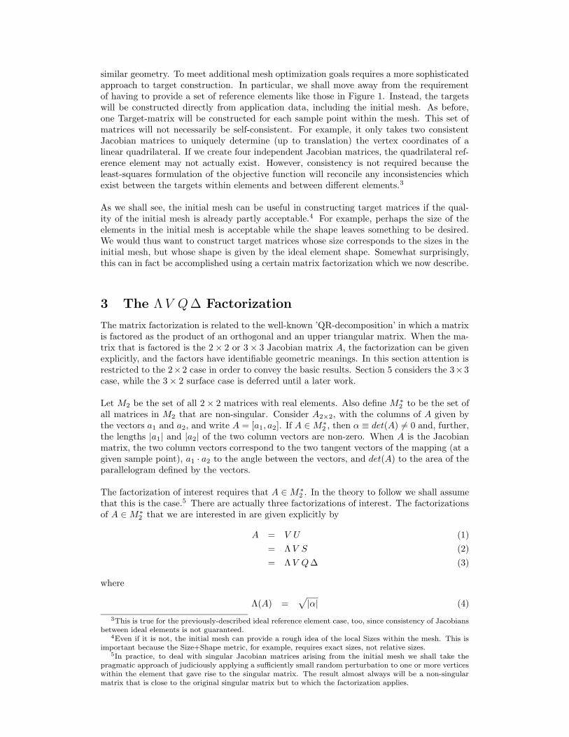
similar geometry. To meet additional mesh optimization goals requires a more sophisticatedapproach to target construction. In particular, we shall move away from the requirementof having to provide a set of reference elements like those in Figure 1. Instead, the targetswill be constructed directly from application data, including the initial mesh. As before,one Target-matrix will be constructed for each sample point within the mesh. This set ofmatrices will not necessarily be self-consistent. For example, it only takes two consistentJacobian matrices to uniquely determine (up to translation) the vertex coordinates of alinear quadrilateral. If we create four independent Jacobian matrices, the quadrilateral ref-erence element may not actually exist. However, consistency is not required because theleast-squares formulation of the objective function will reconcile any inconsistencies whichexist between the targets within elements and between different elements.3

As we shall see, the initial mesh can be useful in constructing target matrices if the qual-ity of the initial mesh is already partly acceptable.4 For example, perhaps the size of theelements in the initial mesh is acceptable while the shape leaves something to be desired.We would thus want to construct target matrices whose size corresponds to the sizes in theinitial mesh, but whose shape is given by the ideal element shape. Somewhat surprisingly,this can in fact be accomplished using a certain matrix factorization which we now describe.

3 The Λ V Q ∆ Factorization

The matrix factorization is related to the well-known ’QR-decomposition’ in which a matrixis factored as the product of an orthogonal and an upper triangular matrix. When the ma-trix that is factored is the 2 × 2 or 3 × 3 Jacobian matrix A, the factorization can be givenexplicitly, and the factors have identifiable geometric meanings. In this section attention isrestricted to the 2×2 case in order to convey the basic results. Section 5 considers the 3×3case, while the 3 × 2 surface case is deferred until a later work.

Let M2 be the set of all 2 × 2 matrices with real elements. Also define M ∗2 to be the set of

all matrices in M2 that are non-singular. Consider A2×2, with the columns of A given bythe vectors a1 and a2, and write A = [a1, a2]. If A ∈M∗

2 , then α ≡ det(A) 6= 0 and, further,the lengths |a1| and |a2| of the two column vectors are non-zero. When A is the Jacobianmatrix, the two column vectors correspond to the two tangent vectors of the mapping (at agiven sample point), a1 · a2 to the angle between the vectors, and det(A) to the area of theparallelogram defined by the vectors.

The factorization of interest requires that A ∈M ∗2 . In the theory to follow we shall assume

that this is the case.5 There are actually three factorizations of interest. The factorizationsof A ∈M∗

2 that we are interested in are given explicitly by

A = V U (1)

= ΛV S (2)

= ΛV Q∆ (3)

where

Λ(A) =√

|α| (4)

3This is true for the previously-described ideal reference element case, too, since consistency of Jacobiansbetween ideal elements is not guaranteed.

4Even if it is not, the initial mesh can provide a rough idea of the local Sizes within the mesh. This isimportant because the Size+Shape metric, for example, requires exact sizes, not relative sizes.

5In practice, to deal with singular Jacobian matrices arising from the initial mesh we shall take thepragmatic approach of judiciously applying a sufficiently small random perturbation to one or more verticeswithin the element that gave rise to the singular matrix. The result almost always will be a non-singularmatrix that is close to the original singular matrix but to which the factorization applies.

©©©©

©©©©©©

©©©©

©©©©

©©*r1

y

£££££££££££££±

r2

xθ

φ

Figure 2: The vectors a1 = r1 (cos θ, sin θ) and a2 = r2 (cos(θ + φ), sin(θ + φ)).

is a scalar, and the remaining factors are the 2 × 2 matrices:

V (A) =

[

a1

|a1|,−(a1 · a2) a1 + |a1|2 a2

|α| |a1|

]

(5)

Q(A) =

√

|a1| |a2||α|

(

1 a1·a2

|a1| |a2|0 |α|

|a1| |a2|

)

(6)

∆(A) =1

√

|a1| |a2|

(

|a1| 00 |a2|

)

(7)

S(A) =1

√

|α|

(

|a1| a1·a2

|a1|0 |α|

|a1|

)

(8)

U(A) =

(

|a1| a1·a2

|a1|0 |α|

|a1|

)

(9)

The explicit factorizations show that, given A non-singular, the 2 × 2 matrices V , Q, ∆,S = Q∆, and U = ΛS are determined, as is the scalar Λ. This factorization of the mesh Ja-cobian was first mentioned in [9]. Note that the matrix factors themselves are non-singular.

The factors of A have recognizable geometric meanings. This is more easily seen if wereplace the column vectors a1 and a2 in A = [a1, a2] with the geometric quantities r1 = |a1|,r2 = |a2|, θ, and φ shown in Figure 2. Then φ is the angle between the two column vectorsand θ is the angle between the first column vector and the x-axis. Let the Jacobian-matrixthus be given by

A =

(

r1 cos θ r2 cos(θ + φ)r1 sin θ r2 sin(θ + φ)

)

Then det(A) = r1 r2 sinφ. The factorization thus exists provided r1 6= 0, r2 6= 0, φ 6= 0, andφ 6= π. Moreover, the conditions r1 > 0, r2 > 0, and 0 < φ < π ensure that A has a positivedeterminant and thus V will be a rotation matrix, rather than a flip.

Applying the factorization formulas to the previous form of A, and assuming det(A) > 0,we obtain

Λ =√

r1 r2 sinφ

V =

(

cos θ − sin θsin θ cos θ

)

Q =1√sinφ

(

1 cosφ0 sinφ

)

∆ =

√

r1

r2

0

0√

r2

r1

S =1√

r1 r2 sinφ

(

r1 r2 cosφ0 r2 sinφ

)

U =

(

r1 r2 cosφ0 r2 sinφ

)

From this factorization, we see that Λ is the square root of the local area of the mapping.Λ ≥ 0, is related to area and has units of length; we refer to Λ as the local Size parameter.The matrix V is dimensionless and is a rotation, i.e., det(V ) = 1 and V tV = I.6 Becausethe first column of V is the unit vector in the direction a1, we see that V is related tothe local Orientation of the map with respect to the coordinate system. The matrix Q isdimensionless, upper triangular, has unit determinant, equal-length columns, and positivediagonal elements. Because Q can be written in terms of the sine and cosine of the anglebetween the vectors a1 and a2, we see that it is related to local angle or Skew between thetangents. The matrix ∆ is dimensionless, diagonal, with positive diagonal elements, andunit determinant. Because the diagonal elements of ∆ are ratios of the lengths of the twotangent vectors, we see that it is related to local aspect ratio. The matrix S is dimensionless,upper triangular, has positive diagonal entries, and unit determinant. As the product ofskew and aspect ratio matrices, S is related to the local shape. The matrix U has units oflength, is upper triangular, has positive diagonal entries, and its determinant is |α|. As theproduct of Size and Shape quantities, we see that U is related to local Shape+Size.

To understand how this factorization can be used in target construction, recall the examplegiven at the end of the previous section, in which the initial mesh had good Size quality, butpoor Shape quality. The factorization shows that we can factor the Jacobian matrices be-longing to the initial mesh into two matrices ΛV and S such that Ainit = (Λinit Vinit)Sinit.To construct an appropriate Target matrix, we discard Sinit and replace it with Snew, thelatter representing the desired local Shape. The Target-matrix is then W = Λinit Vinit Snew.A key question is: under what conditions is S(W ) = Snew, i.e., how can one construct Snew

such that the Shape implied by the Target is the shape specified by Snew?

To investigate this question, define the following matrix sets in M ∗2 :

• V is the set of all orthogonal matrices, R is the set of all rotations, F is the set of allflips. The union of the latter two is V,

• U is the set of all upper triangular matrices with positive diagonal elements,

• S is the set of all matrices in U having unit determinant,

• Q is the set of all matrices in S having equal length columns,

• D is the set of all diagonal matrices in S

One can see by inspection of (4)-(9) that V (A) ∈ V, U(A) ∈ U , S(A) ∈ S, Q(A) ∈ Q, and∆(A) ∈ D.

Proposition 1.First, det(A) > 0 if and only if V (A) is a rotation. Second, det(A) < 0 if and only if V (A)is a flip.Proof.

6Our choice of r1, r2, and φ eliminated the possibility that V could be a flip.

From (1) we see that α = det(A) = det(V ) det(U) = det(V ) |α|. Thus, if det(A) > 0, wemust have det(V ) = 1 and, because V is either a flip or a rotation, V must be a rotation.If, on the other hand, V is a rotation, then det(V ) = 1, and so det(A) = |α| > 0. The proofof the second statement is similar. §

Given A ∈ M∗2 , the matrices V , Q, ∆, etc. are uniquely determined. For the purpose of

target construction, the key question is the reverse statement: given matrices V ′, U ′, underwhat conditions is V (V ′U ′) = V ′, U(V ′U ′) = U ′?

Proposition 2.If V ′ ∈ V, U ′ ∈ U , and A′ = V ′ U ′, then V (A′) = V ′ and U(A′) = U ′.Proof

The proof for V ′ ∈ R is provided here, while the case V ′ ∈ F is similar. Note first thatdet(U ′) > 0 since the determinant of an upper triangular matrix is the product of thediagonal entries and these are assumed positive. Since det(V ′) = 1, we have det(A′) =det(U ′) > 0. Thus A′ ∈ M∗

2 and the factorization A′ = V (A′)U(A′) exists. Therefore, wehave

V ′ U ′ = V (A′)U(A′)

From this, det(V ′) det(U ′) = det[V (A′)] det[U(A′)]. But det(V ′) = 1, det(U ′) > 0, anddet[U(A′)] = |det(A′)| > 0. Therefore, det[V (A′)] > 0, and so we must have det[V (A′)] = 1and V (A′) is a rotation. Since both V ′ and V (A′) are rotations, the product (V ′)tV (A′) isalso a rotation. Hence U ′ is a rotation matrix times U(A′). The fact that both of the latterare upper triangular with positive diagonal entries forces (V ′)tV (A′) = I. That being thecase, one must have V (A′) = V ′ and U(A′) = U ′. §

Proposition 2 shows that the conditions V ′ ∈ V and U ′ ∈ U are sufficient to guarantee thestated result. It is easy to see that they are necessary as well. Proposition 2 says, in effect,that the factorization into matrices belonging to the defined sets is unique.

Proposition 3.Suppose Λ′ > 0, V ′ ∈ V, and S′ ∈ S. If A′ = Λ′ V ′ S′, then Λ(A′) = Λ′, V (A′) = V ′ andS(A′) = S′.Proof.The proof for V ′ ∈ R is provided, while the case V ′ ∈ F is similar. Note first that,det(A′) = (Λ′)2 det(V ′) det(S′). Because V ′ ∈ V, det(V ′) = 1. In addition, S′ ∈ S givesdet(S′) = 1. Therefore, det(A′) = (Λ′)2 > 0. In turn, this means A′ ∈ M∗

2 and so the thefactorization A′ = Λ(A′)V (A′)S(A′) exists. Thus, we have

Λ′ V ′ S′ = Λ(A′)V (A′)S(A′)

By definition, Λ(A′)S(A′) = U(A′). Further, if we let U ′ = Λ′ S′, we see that U ′ is uppertriangular with positive diagonal entries, so U ′ ∈ U . Thus, A′ = V ′ U ′ and Proposition 2can be applied to show V ′ = V (A′) and U ′ = U(A′). The latter gives

Λ′ S′ = Λ(A′)S(A′)

Taking the determinant of both sides of the expression and equating, we find that, [Λ′]2 =[Λ(A′)]2. But since both of these scalars are positive, that means Λ′ = Λ(A′). Then,S′ = S(A′) is immediate. §

The assumptions in Proposition 3 are both sufficient and necessary to guarantee the statedresults.

Proposition 4.Suppose Λ′ > 0, V ′ ∈ V, Q′ ∈ Q, and ∆′ ∈ D. If A′ = Λ′ V ′Q′ ∆′, then Λ(A′) = Λ′,V (A′) = V ′, Q(A′) = Q′, and ∆(A′) = ∆′.Proof.

The proof for V ′ ∈ R is provided, while the case V ′ ∈ F is similar. We have det(A′) = (Λ′)2

because V ′ ∈ V, Q′ ∈ Q, and ∆′ ∈ D requires that these matrices have unit determinant.Thus A′ is non-singular and the factorization exists, i.e., A′ = Λ(A′)V (A′)Q(A′)D(A′).Therefore

Λ′ V ′Q′ ∆′ = Λ(A′)V (A′)Q(A′)∆(A′)

By definition, Q(A′)∆(A′) = S(A′). Further, if we let S′ = Q′ ∆′, we see that S′ ∈ S.Thus, A′ = Λ′ V ′ S′ and Proposition 3 can be applied to show Λ(A′) = Λ′, V (A′) = V ′, andS(A′) = S′. The latter gives

Q′ ∆′ = Q(A′)∆(A′)

Multiplying the matrices on each side of this relation and equating the elements reveals thatQ′ = Q(A′) diag(r, 1/r) for some r > 0. But since the columns of Q′ have equal length, somust the columns of the product Q(A′) diag(r, 1/r). This forces r = 1, and thus diag(r, 1/r)is the identity matrix. Therefore, Q(A′) = Q′. It is then immediate that ∆(A′) = ∆′. §

The assumptions in Proposition 4 are both sufficient and necessary to guarantee the statedresults.

Corollary.Let Gk ∈M∗

2 with k = 1, 2, 3, 4, and let G = Λ(G1)V (G2)Q(G3)∆(G4). Then

Λ(G) = Λ(G1)

V (G) = V (G2)

Q(G) = Q(G3)

∆(G) = ∆(G4)

Proof.From prior observations, Λ(G1) > 0, V (G2) ∈ V, Q(G3) ∈ Q, and ∆(G4) ∈ D. ApplyingProposition 4, we have the stated result. §

Similarly corollaries may be proved using Propositions 2 and 3. For example, if G1 ∈ M∗2 ,

G2 ∈M∗2 , and G = V (G1)U(G2), then V (G) = V (G1) and U(G) = U(G2).

4 Target-matrix Construction Using the 2 × 2 Factor-ization

The propositions in the previous section justify the following approach to Target-matrixconstruction. Given an initial mesh, a set of matrices Ainit can be created from the under-lying mappings. If Ainit ∈ M∗

2 , then from the expressions (4)-(9), initial values Vinit =V (Ainit), Uinit = U(Ainit), etc., can be found such that

Ainit = Vinit Uinit

= Λinit Vinit Sinit

= Λinit VinitQinit ∆init

To construct Target-matrices from these factorizations, one or more of these initial matrixfactors can be replaced with a new matrix. For example, if we set W = Λinit Vinit Snew,then according to the propositions, Λ(W ) = Λinit, V (W ) = Vinit, and S(W ) = Snew, pro-vided Snew ∈ S. If this target were used along with the local metric |T − I|2, optimizationshould produce an optimal mesh whose shape quality is now close to Snew, while the Sizeand Orientation qualities would remain close to those of the initial mesh.

It is clear that many different combinations of new and initial matrices can be created andcombined to form a target matrix. For the moment, let us leave aside the question of whatcombinations exist, and which are important, to focus instead on how one might createuseful λnew, Vnew, Qnew, ∆new, Snew, and Unew matrices.

The initial matrices Vinit, etc., will in general vary from one sample point in the mesh toanother. To realize the full potential of the Target-matrix paradigm, the new matrices Vnew,etc., must also be allowed to vary over the sample points. Let (Vnew)k denote the new Ori-entation matrix at sample point k, and use similar notation for the other matrices.

The following subsections provide high-level methods for creating new matrices that belongto the proper sets V, etc., so that the Propositions of the previous section hold. Notably,the matrix factors are created from data available to the application. This data, of course,varies from one application to the next. Most prior methods of mesh optimization do notuse the data to be described below, at least not in such a systematic fashion. Thus, tar-get construction based on this seldom-used data potentially permits the creation of betteroptimal meshes. Of course, Target-matrix creation is an art because the ingenuity of thecreator plays an important role in the quality of the results.

4.1 The Size Factor (Λnew)k

Recall that the Size factor Λ(A) =√

|α| is related to the local area of the map. Clearly,if the application desires a relatively large element in some location, then Λ should be rel-atively large. The area, in turn, depends on the lengths and included angle between thelocal tangent vectors. If the angle φ is controlled via the Q-matrix, so that sinφ ≈ 1, thenΛ roughly controls the geometric average of the lengths of the tangents. These, in turn, arerelated to the lengths of the edges in an element.

A generic model for calculating the Size factor over the set of sample points in the meshassumes that we are given application data such that a set of positive scalars {fk} definedat the sample points can be computed. If there are K sample points in the mesh, letf̄ = 1

K

∑

k fk be the average value over the set of values. Further, given (Λinit)k as thevalue of Λ at each sample point of the initial mesh, let Λ̄ = 1

K (Λinit)k be the average Sizein the initial mesh. A properly-scaled model for a new Size factor is

(Λnew)k =

(

fk

f̄

)

Λ̄ (10)

This model will tend to create Sizes in the optimal mesh that are proportional to fk. Notethat this scaling is such that 1

K

∑

k(Λnew)k = Λ̄, so that the average Λ in the optimal meshis the same as in the initial mesh. This property helps ensure the mesh remains of goodquality. The requirement that f be a positive function comes from the fact that we need Λpositive in order for the factorization Propositions to hold. When fk ≡ 1 over all the samplepoints, we have the special case (Λnew)k = Λ̄, which corresponds to the goal of creating amesh with equal Size everywhere.7

If Size is important to control while optimizing the mesh, then of course, one must notuse a size-invariant local metric such as the Shape metric. The Size+Shape metric or theSize+Shape+Orientation metrics are logical candidates.

Applications may have available the following data which can be used to create useful {fk}:

• a posteriori discretization error estimates or error indicator data,

• scalars derived from physically-meaningful scalar fields such as conductivity, perme-ability, depth contours, etc.,

7Another special case is obtained by letting fk = (Λinit)k, which gives (Λnew)k = (Λinit)k.

• determinants of symmetric positive definite matrices such as a the solution Hessian,the thermal conductivity, the Permeability tensor, etc.,

• the norm of the solution gradient, or

• surface curvature.

It is evident from these examples that a wide variety of application-specific Size-adaptedoptimal meshes can potentially be created.

4.2 The Orientation Factor (Vnew)k

Recall that the Orientation matrix V is related to the angle θ that the first column of Amakes with the x-axis. If the angle φ is controlled by the Q-matrix, then V additionallycontrols the local orientation of the tangent vectors to the map with respect to the globalcoordinate system.

A generic model for calculating a new Orientation matrix to be used in the Target assumesthat we are given application data from which a set of non-zero vectors {(uk, vk)} defined atthe sample points can be computed. Let cos θk = uk/

√

u2k + v2

k and sin θk = vk/√

u2k + v2

k,so that

(Vnew)k =1

√

u2k + v2

k

(

uk −vk

vk uk

)

(11)

With this construction, Vnew is a rotation, and the optimal mesh should tend to align thefirst column of the Jacobian matrix of the optimized mesh with the vector field at eachsample point.

In some cases, one may wish to align the second column of the Jacobian matrix with thevector field. To do so, we propose

(Vnew)k =1

√

u2k + v2

k

(

vk uk

−uk vk

)

(12)

If Orientation is important to control while optimizing the mesh, then of course, one mustnot use an orientation-invariant local metric such as the Shape or Size+Shape metrics. TheSize+Shape+Orientation metric is the proper choice.

Applications may have available, among other possibilities, the following data which can beused to create useful {(uk, vk)}: magnetic fields, fluid velocity vectors, solution gradients,fluxes, or eigenvectors of symmetric tensor fields. It is evident from these examples that awide variety of application-specific Orientation-adapted optimal meshes can potentially becreated.

This approach was originally suggested in [11], prior to the TMP.

It is important to note that, to use this approach effectively requires knowledge of the way inwhich the vertices of each mesh element are labeled. An example is given in Figure 3. In theterminology of [5], V is not a label-invariant quantity, whereas Λ is. The issue is not a majordifficulty for structured meshes since the labeling is often consistent from one element tothe next, but can be troublesome on unstructured meshes because an incorrect assumptionon the labeling could result in a tangled mesh. Moreover, in practice, orientation-controlseems to be less commonly wanted with unstructured meshes because such meshes do nothave global tangent lines.

x

y

0 1

23

e1

e2

»»»»»»

»: v

Figure 3: A sample point located at vertex 0 of the element shown has the first column of Aequal to e1 assuming the labeling shown. However, if the labeling is cyclically permuted, sothat 0123 becomes 3012, then the sample point at vertex 0 has the first column of A equalto e2. Thus, depending on the labeling, either e1 or e2 would align with v.

4.3 The Skew Factor (Qnew)k

Recall that the Skew-matrix is related to the angle φ between the two tangent vectors ofthe map. Assume that we are given application data such that the set of angles {φk} (withsinφk > 0) over all sample points can be computed. The generic model for calculating anew Skew-matrix is based directly on the geometric definition of Q given in the previoussection:

(Qnew)k =1√

sinφk

(

1 cosφk

0 sinφk

)

(13)

The condition on sinφk helps meet the conditions for the factorization Propositions to hold.

In practice, many applications may not be able to supply meaningful data from which wecan calculate the set {φk}, varying over the sample points. One remedy is simply to setφk to a constant angle which is related to the angle found in the ideal element type. Forexample, the ideal quadrilateral element has φ = π/2, which results in (Qnew)k = I. Theideal triangle element has φ = π/3, giving

(Qnew)k =1√

2 4√

3

(

2 1

0√

3

)

(14)

The use of constant Q matrices in the Target is appropriate if a goal of the optimization isto create a mesh whose local tangents all include the ideal angle.

None of the local metrics in the Target-matrix paradigm are invariant to the skew-angle, soQnew can be used with any metric.

4.4 The Aspect Ratio Factor (∆new)k

Recall that the ∆-matrix is related to the local tangent aspect ratio√

r1

r2

. A generic model

for calculating the Aspect Ratio matrix over the set of sample points in the mesh assumesthat we are given application data such that a set of positive scalars {ρk} defined at the

sample points can be computed. Then let

(∆new)k =

( √ρk 00 1/

√ρk

)

(15)

An important special case occurs with ρk ≡ 1 for all k. Then (∆new)k = I, which is appro-priate if one desires that the optimal mesh be isotropic.

None of the local metrics in the Target-matrix paradigm are invariant to aspect ratio, so∆new can be used with any metric.

Applications may have available, among other possibilities, the following data which can beused to create useful values of ρk: the eigenvalues of a symmetric positive definite matrixsuch as the Hessian, the Curvature, or the Diffusivity, a priori knowledge such as the aspectratio of the geometric domain or the aspect ratio of a boundary layer, or pairs of vectorssuch as the electric and magnetic field vectors.

As with Orientation, Aspect-Ratio is not label-invariant. Thus, in Figure 3, the aspect-ratioat vertex 0 is r1/r2 is e1/e2 when the labeling of the element vertices is as shown, whereas,the aspect-ratio at vertex 0 becomes e2/e1 under the label permutation 0123 → 3012. There-fore, to use this approach to aspect-ratio effectively requires specific knowledge of the wayin which the vertices of each mesh element is labeled.

4.5 The Shape and Shape+Size Factors (Snew)k, (Unew)k

Recall that the Shape matrix is related to both angle and aspect ratio. A generic modelfor calculating a new Shape matrix is to take advantage of the relation Snew = Qnew∆new.Therefore, a new Shape matrix is found by first calculating new Skew and Aspect Ratiomatrices according to the previous two subsections, and then multiplying them together.

The same approach can be used to calculate a new Size+Shape matrix Unew = ΛnewSnew.

4.6 Creating New Factors by Multiplying Initial Factors

In the preceding subsections, we presented an approach to Target construction in which new

factors, created from application data, are substituted for initial factors. The initial factorsare thus discarded. New factors can also be created by modification of the initial factors.This may be a more convenient way to construct Targets in certain situations.

The basic idea is the following: let λk > 0, Vk ∈ V, Dk ∈ D be calculated from data suppliedby the application, for all k. Then define new factors in terms of the initial factors as follows:

(Λnew)k = λk (Λinit)k

(Vnew)k = Vk (Vinit)k

(∆new)k = (∆init)k Dk

where Λinit = Λ(Ainit), Vinit = V (Ainit), and ∆init = ∆(Ainit). These operations arepossible because the sets V and D are closed under multiplication.8 The new factors thenreplace the initial factors, as before. For example, if one desired W = Λinit Vnew Qnew ∆init,then this method of creating new factors gives

Wk = (Λinit)k (Vnew)k (Qnew)k (∆init)k

= (Λinit)k Vk (Vinit)k (Qnew)k (∆init)k

8The sets S and U are also closed, so a similar approach can be taken to create Snew or Unew from Sinit

or Uinit. However, the set Q is not closed under multiplication, so this approach cannot be taken with theSkew factor.

with V (Wk) = Vk (Vinit)k. One can also create a new Jacobian matrix from the initial

Jacobian matrix by letting

(Anew)k = λk Vk (Ainit)k Dk

This would be used in the Target Wk = (Anew)k. The construction can be written

(Anew)k = [λk (Λinit)k] [Vk (Vinit)k] (Qinit)k [(∆init)k Dk]

Because the sets are closed, the Propositions allow us to conclude that

Λ[(Anew)k] = λk (Λinit)k

V [(Anew)k] = Vk (Vinit)k

∆[(Anew)k] = (∆init)k Dk

Usually, Vk will be a rotation, but if, at a particular sample point, (Vinit)k is a flip, thenperhaps choosing Vk to be a flip might be effective in eliminating an inverted element. Infact, this choice is necessary since we require that all Target-matrices have positive deter-minant.

If a reference mesh is available, then one could use λk = Λ(Aref ), Vk = V (Aref ), and/orDk = ∆(Aref ).

It is unclear if this approach to creating new factors by modifying the initial factors is usefulin practice. In a later section, we see that cases involving one or more of λk, Vk, or Dk beingconstant could be of use in mesh Morphing or Copying.

4.7 Closing Remarks on the Factorization Approach to Target Con-struction

In summary, given appropriate application data, the generic models of the previous subsec-tions can be used to compute new matrix factors to be used in combination with the initial

matrix factors to construct Target-matrices over the set of sample points such that a particu-lar mesh optimization goal is met. A Target combination such asW = Λinit Vnew Qnew ∆init,for example, when used with the Size+Shape+Orientation local metric, essentially says thatthe goal is to preserve the initial mesh qualities related to Size and Aspect Ratio, while im-

proving the qualities related to Orientation and Skew. Thus, in TMP, one can, as a goal,both preserve and improve various mesh qualities via optimization.

As noted Section Two, it is not necessary that the set of Target-matrices constructed fromthe factorization method be consistent from one sample point to another because the least-squares objective function will reconcile the inconsistencies. However, the more consistentthe set of Targets is, the more likely the optimal mesh will satisfy the optimization goalimplied by the targets.

Two additional methods for creating new matrix factors should be mentioned.

First, if a reference mesh is available, one can compute the factorization Aref = Λref Vref Qref ∆ref .Then one can let, for example, Λnew = Λref , Vnew = Vref , etc. Hence, one can have Target-matrices with combinations such as W = Λref Vinit Snew in which the target is composed ofinformation from the reference mesh, the initial mesh, and from application-specific data.This example would make sense if the reference mesh has good Size quality, but poor Shapequality.

Second, a similar approach can be taken that involves a two-stage optimization procedurein which the optimal mesh from the first stage is used to create targets for the second stage.For example, an optimal mesh could first be created by successively optimizing local patches

from the initial mesh using a Shape metric with target based on the ideal element shape.After each local patch has been optimized one calculates (Aopt)k. The optimization contin-ues to the next local patch, but not before restoring the coordinates of the center vertexfrom the optimized local patch to its initial position. This is followed by a subsequent globaloptimization, again beginning with the initial mesh, but using the Size+Shape+Orientationmetric, and the target W = Aopt to create a mesh that is similar to the initial mesh,but with better shape quality. This method was proposed in the ALE rezone paper [12].Other possibilities involving factorization of the Jacobian matrix of optimal mesh resultingfrom the first optimization stage to obtain new matrix factors that can be inserted into thesecond-stage target-matrices may be useful.

In principle, there is nothing to prevent one from varying the combination of initial andnew matrix factors from one sample point to the next. For example, the sample pointsin one subset of the mesh elements might use W = Ainit, while another subset might useW = Anew. Such a possibility raises the issue of Target-matrix smoothness. Numericalexperiments in the past suggest that if the Targets do not vary smoothly over the set ofsample points, the optimal mesh will not be smooth.9 A combination of initial and new tar-gets is likely to be non-smooth unless carefully done, so this possibility may be unattractivefor that reason. The same can be said concerning the matrix factors, i.e., they should varysmoothly over the sample points if a smooth optimal mesh is wanted.

5 Extension of the Factorization to Three Dimensions

Sections 3 and 4 focused on 2× 2 matrices. In this section the results are extended to 3× 3matrices, which are associated with volume mesh elements.

Let M3 be the set of all 3 × 3 matrices with real elements, and let M ∗3 be the set of non-

singular matrices in M3. Consider A3×3, with the columns of A given by the vectors a1, a2,and a3, and write A = [a1, a2, a3]. If A ∈M∗

3 , then α ≡ det(A) 6= 0 and thus the quantities|a1|, |a2|, |a3|, and |a1 ×a2| are non-zero. When A is the Jacobian matrix, the three columnvectors correspond to the three tangent vectors of the mapping (at the given sample point).

For A ∈M∗3 , the factorizations (1)-(3) still hold, provided

Λ(A) = |α|1/3 (16)

V (A) =

(

a1

|a1|,−(a1 · a2)a1 + |a1|2a2

|a1||a1 × a2|,α(a1 × a2)

|α||a1 × a2|

)

(17)

Q(A) = 3

√

|a1||a2||a3||α|

1 a1·a2

|a1||a2|a1·a3

|a1||a3|0 |a1×a2|

|a1||a2|(a1×a2)·(a1×a3)|a1×a2||a1||a3|

0 0 |α||a1×a2||a3|

(18)

∆(A) =1

3

√

|a1||a2||a3|

|a1| 0 00 |a2| 00 0 |a3|

(19)

S(A) =1

3

√

|α|

|a1| a1·a2

|a1|a1·a3

|a1|0 |a1×a2|

|a1|(a1×a2)·(a1×a3)

|a1×a2||a1|0 0 |α|

|a1×a2|

(20)

U(A) =

|a1| a1·a2

|a1|a1·a3

|a1|0 |a1×a2|

|a1|(a1×a2)·(a1×a3)

|a1×a2||a1|0 0 |α|

|a1×a2|

(21)

9The experiments also suggest that, while target-smoothness is necessary for a smooth optimal mesh, itmay not be sufficient.

The matrices above belong to the sets V, U , S, Q, and D defined in Section 3, but now onM∗

3 .10

The factors of A = [a1, a2, a3] again have recognizable geometric meanings. Let ri = |ai|and ψij , (i, j) ∈ {1, 2, 3}, be the included angle between ai and aj , and further assume thatfor j 6= i, 0 < ψij < π so that the determinant of A will be positive. Let ν be the anglebetween the vectors a1 × a2 and a1 × a3. Then one can show

cos ν =cosψ23 − cosψ12 cosψ13

sinψ12 sinψ13

sin ν =α

r1 r2 r3 sinψ12 sinψ13

Then the factorization above becomes

Λ(A) = |α|1/3

V (A) =1

sinψ12

(

a1

r1sinψ12,

a2

r2− a1

r1cosψ12,

a1

r1× a2

r2

)

Q(A) = 3

√

r1 r2 r3|α|

1 cosψ12 cosψ13

0 sinψ12 sinψ13 cos ν0 0 sinψ13 sin ν

∆(A) =1

3√r1 r2 r3

r1 0 00 r2 00 0 r3

S(A) =1

3

√

|α|

r1 r2 cosψ12 r3 cosψ13

0 r2 sinψ12 r3 sinψ13 cos ν0 0 r3 sinψ13 sin ν

U(A) =

r1 r2 cosψ12 r3 cosψ13

0 r2 sinψ12 r3 sinψ13 cos ν0 0 r3 sinψ13 sin ν

As in the 2D case, the quantities Λ, V, Q, and ∆ can be seen to be related to size, orienta-tion, skew, and aspect ratio, respectively.

Proposition 1 from Section 3 holds for d = 3 as well as d = 2, as can be seen from are-reading of the proof. Changing M ∗

2 to M∗3 in the proof of Proposition 2 gives a valid

proof that the proposition also holds for d = 3. With minor modifications to the proofs ofPropositions 3, 4, and 5, one can show that these also hold for d = 3.

6 Target-matrix Construction using the 3×3 Factoriza-tion

The main difference between this section and Section 4 is due to the different explicit ΛV Q∆factorizations for 2×2 and 3×3 matrices. Thus, the emphasis in this section is on a descrip-tion of the generic models for the new matrices in the factorization of 3×3 Jacobian matrices.The models rely heavily on the expressions given at the end of the previous section. Theapproach described in subsection 4.6 carries over immediately to the three-dimensional case.

6.1 The Size Factor (Λnew)k

The Size factor when d = 3 is related to the local volume of the map at a sample point. Thegeneric model is identical to that given in Section 4, as are the sources for the application

10The identity |α||a1| ≡ |(a1 × a2) × (a1 × a3)| is useful in showing that the lengths of the columns of Q

are equal.

data used to determine {fk}.

6.2 The 3 × 3 Orientation Factor (Vnew)k

To determine a new 3 × 3 orientation matrix requires two non-zero vectors {uk} {vk} ateach sample point, with |uk × vk| 6= 0. Then the generic model is the rotation

(Vnew)k =

[

uk

|uk|,|uk|2 vk − (uk · vk)uk

|uk| |uk × vk|,

uk × vk

|uk × vk|

]

This will tend to make the optimal mesh align with the two vector fields such that the firstcolumn of the Jacobian will align with u and the second column with v.

To align the second and third columns of the active Jacobian matrix with the pair of vectorsu and v, respectively, let

(Vnew)k =

[

uk × vk

|uk × vk|,

uk

|uk|,|uk|2 vk − (uk · vk)uk

|uk| |uk × vk|

]

and to align the third and first columns of the active Jacobian matrix with the pair of vectorsu and v, respectively, let

(Vnew)k =

[ |uk|2 vk − (uk · vk)uk

|uk| |uk × vk|,

uk × vk

|uk × vk|,

uk

|uk|

]

Applications may have available, among other possibilities, the following data which can beused to create useful pairs uk, vk: electric and magnetic fields, or eigenvectors of matrices.In practice, the application may have access to only one vector field, so some ingenuity willbe required to find a suitable second field.

V3×3 is not a label-invariant quantity, so some effort is needed to properly correlate elementvertex numberings with the desired alignment.

6.3 The 3 × 3 Skew Factor (Qnew)k

The angles ψij refer to the angles between the vector triple consisting of the columns ofthe Jacobian matrix at a sample point. A generic model for (Qnew)k could be based onthese angles, according to the Skew matrix factor of the previous section. In practice, fewapplications will be able to supply these angles at all the sample points. More useful per-haps is the case where Qnew is a constant which is based on the angles in the ideal element.For example, in a hexahedral element, the face angles are all π/2 so that (Qnew)k = I atall the sample points. The use of constant Skew matrices in the Target is appropriate ifa goal of the optimization is to create a mesh whose local tangents all include the ideal angle.

For a tetrahedral element, the face angles are all π/3, giving

(Qnew)k =6√

2

1 12

12

0√

32

√3

6

0 0√

23

For a triangular wedge element, with face angles ψ12 = π3 and ψ23 = ψ13 = π

2 ,

(Qnew)k =

1 12 0

0√

32 0

0 0 1

For a square pyramid element of height h and base edge-length `, let

r =

√

1 +1

2

(

`

h

)2

and

(Qnew)k = 3√r

1 0 `2rh

0 1 `2rh

0 0 1r

6.4 Aspect Ratio Schemes (∆new)k

A generic model for ∆ requires that we be given three sets of positive numbers {(r1)k},{(r2)k}, {(r3)k} at each sample point, representing relative lengths of the three tangentvectors. The model is

∆new =

3

√

r2

1

r2 r3

0 0

0 3

√

r2

2

r3 r1

0

0 0 3

√

r2

3

r1 r2

For an isotropic mesh, we can use ∆new = I, otherwise, element labeling must be taken intoaccount in order for the results to be close to what is desired.

7 Example of Target Construction using ΛV Q∆

A fore-runner of the Target-matrix paradigm can be found in [10], in which a two-dimensionalstructured mesh based on a global map is aligned with a given vector field. The optimizationis cast as a problem in the calculus of variations and the metric |A−1 −W−1|2 is used. Thetarget was calculated directly and did not use the factorization method given in the presentpaper. However, the approach was similar to the construction of Vnew given here. Many ofthe concepts in the present TMP were lacking in the original alignment paper, such as thefactorization, the extension to finite element meshes, the weighted Jacobian matrix T , theconcept of barrier metrics, and the use of Shape or Shape+Size metrics.

An example of the factorization method described in Sections 3 and 4 is given in this section.The initial mesh consists of a quadrilateral ’paved’ planar region. The mesh is isotropic,with good shape quality (see Figure 4). The difficulty with this mesh is that there are anumber of edges located near the domain corners which have relatively small edge-lengths.The simulation code that used the mesh is explicit in time, so these small edge-lengths con-trol the size of the time-step via the Courant condition. The goal, then, of the optimizationis to make the edge-lengths in the mesh more uniform so that a larger time-step can be taken.

The Target-matrix paradigm lends itself readily to this problem. To construct the set ofTarget-matrices we begin with the initial mesh, calculate the Jacobian matrix Ainit at eachsample point. The sample points consist of the four corners of each quadrilateral in the mesh.Apply the ΛV Q∆ factorization to obtain the factors Λinit, Vinit, Qinit, and ∆init. The factorwhich most needs to be replaced with a ’new’ factor is Λinit because this is the primarysource of the non-uniformity in edge-length. To elaborate: Vinit controls only orientation,while Qinit and ∆init are close to uniform since all the elements’ shapes are close to beingsquares. Therefore, we replace Λinit with Λnew as given in Section 4.1. Since uniformity inedge-length is desired, we choose fk ≡ 1 for all k, giving (Λnew)k = Λ̄. Although perhaps

not strictly necessary, we also replace Qinit and Dinit with Qnew = I and Dnew = I in orderto further improve Shape. The constructed Target-matrices are therefore

Wk = Λ̄ (Vinit)k

Because element orientation is not important in this problem, Vinit need not necessarilybe preserved; therefore, we can use an orientation-invariant local metric, which allows theoptimization to adjust orientation if necessary to achieve greater uniformity of edge-lengths.We cannot use a Shape metric, however, because these are insensitive to Λ. Thus, thebest choice of local metric is to use a Size+Shape metric. This choice should preserve (orslightly improve) the square shape of the quadrilaterals while equidistributing the Size (andtherefore, the edge-lengths).11 Because the initial mesh is non-inverted, we can use thebarrier form of the Size+Shape metric to guarantee the optimal mesh is also non-inverted.The local quality metric used to produce the optimized mesh in Figure 4 was the followingbarrier-based 2D Size+Shape metric:

µ(T ) =|T |2 − 2

√

|T |2 + 2τ + 2

2τ

From the figure one sees that indeed the optimal mesh has more uniform edge-lengths. Infact, the minimum edge-length in the optimized mesh is 1.7 times longer that the minimumedge-length in the initial mesh, thus permitting the simulation code to increase the time-stepby the same factor.

The assumptions that went into the design of this optimization and Target constructionmethod are that (1) the initial paved mesh is non-inverted (and thus a barrier-metric canbe used), (2) the elements are quadrilaterals (so that Qnew = I is appropriate), and (3) theelements are isotropic so that Vinit need not be replaced and so that ∆new = I is appro-priate. These assumptions are usually reasonable when the initial mesh is obtained via apaving algorithm. Obviously, if these assumptions are violated, we would need to re-thinkthe Target construction. For example, if the paved mesh consisted of triangular elements,a different Qnew is needed. Or, if the mesh is not isotropic, then perhaps a different ∆new

and Vnew would be needed.

It is noted that there is some flexibility in the Target-construction algorithm for this par-ticular problem. For example, replacing Vinit with Vnew = I might have worked just as wellsince an orientation-invariant metric was used.

The most important point we wish to make is that in the Target-matrix approach, one cangenerally use a very small set of local metrics (Shape, Shape+Size, Shape+Size+Orientation)to address a wide variety of optimization goals. This is accomplished, not by creating newmetrics, but by creating new Target-matrices.

8 Target Construction for Particular Applications

As mentioned earlier, the factorization method of Target construction allows many combi-nations of initial and new matrices. For example, the factorization W = V U gives rise tofour combinations: Vinit Uinit, Vinit Unew, Vnew Uinit, and Vnew Unew. The first is equiva-lent to W = Ainit and the last is equivalent to W = Anew. There are actually even morethan four combinations here because either a new matrix can be created from a genericmodel (like those described in Sections 4 and 6) or it can be created from a reference oroptimized mesh. Additionally, a generic model for a new matrix can often be created us-ing difference types of application data such as scalars, vectors, matrices, or tensors. It isthus difficult to fully enumerate all the possible combinations resulting in Targets within

11A pure Size metric would also equidistribute the edge-lengths, but would not necessarily preserve thesquare shape of the elements.

TMP. Beyond that, there are three local quality metrics, Shape (Sh), Size+Shape (SS),Size+Shape+Orientation (SSO), that can be associated with the different target combina-tions, leading to a large number of possible optimization problems. It turns out that manyof the possible combinations are not particularly useful, so a better approach than directenumeration is needed to find useful combinations.

Instead of trying to enumerate all possible combinations in Target construction, we first list(at an abstract level) the possible uses of each of the four factors in the ΛV Q∆ factorization,beginning with the Size factor, Λ.

The distribution of Size values over the initial and the optimal mesh may be either homo-geneous (constant) or heterogeneous (variable). Except for some special cases, most meshesdo not have a Size distribution which is exactly constant. However, if the Size is nearlyconstant (i.e., the Size distribution has small standard deviation), we shall call the Sizehomogeneous. Four uses of the size factor are identified below:

Sz1. Create a homogeneous Size-distribution (Λnew = constant),

Sz2. Preserve the Size-distribution of the initial mesh (Λinit),

Sz3. Create a particular heterogeneous Size-distribution based on application data (Λnew),or

Sz4. Indifference to size distribution (Λinit or Λ = 1).

One is rarely indifferent to the Size distribution in a mesh. However, we list Sz4 anywaybecause the TMP Shape metrics are invariant to Size, and experience has shown that use ofthe Shape metric generally does not dramatically alter whatever Size distribution is found inthe initial mesh. There are certain applications in which we can take advantage of this sit-uation which are described later in this section. Thus, Sz4 requires the Shape metric, whileSz1-Sz3 can be used with either the Size-Shape metric or the Size-Shape-Orientation metric.

We can similarly list three uses of the Orientation factor:

Or1. Create a particular mesh Orientation (Vnew),

Or2. Preserve the Orientation of the initial mesh (Vinit), or

Or3. Indifference to Orientation (Vinit or V = I).

Indifference to orientation is quite common in applications of mesh optimization, particu-larly if the mesh is isotropic. When one is not indifferent to orientation, one is generallytrying to align the mesh elements with some feature of the solution to a simulation. Manytimes alignment can be achieved simply by conforming the mesh to the boundary of ageometric domain. However, if an Orientation different than that implied by the geome-try is wanted, mesh optimization using Vnew can play a useful role. Or1-Or2 require theSize+Shape+Orientation metric, while Or3 can be used with either Shape or Size+Shapemetrics.

We list three uses of both the Skew and the Aspect Ratio factors.

Sk1. Create a constant Skew based on element type (Qnew = ideal),

Sk2. Preserve the Skew distribution of the initial mesh (Qinit), or

Sk3. Create a particular non-constant Skew distribution (Qnew).

Constant skew means that the Skew-matrix is constant over the set of sample points withinmesh elements of the same type. A hybrid mesh can have constant Skew, meaning that, forexample, all the sample points within triangular elements in the mesh use the Skew-matrixin equation (21), while all the sample points within quadrilateral elements use Q = I.

Table 1: Potential Applications of the Target-matrix Paradigm

App Sz-Goal Data Or-Goal Data AR-Goal Data Metric1 Sz4 initial Or3 initial AR1 ideal Sh2 Sz4 initial Or3 initial AR2 initial Sh3 Sz4 reference Or3 reference AR3 ∆(Aref ) D Sh

4 Sz1 constant Or3 initial AR1 ideal SS5 Sz1 constant Or3 initial AR2 initial SS6 Sz2 initial Or3 initial AR1 ideal SS7 Sz2 initial Or3 initial AR2 initial SS8 Sz3 curvature Or3 initial AR1 ideal SS9 Sz3 error Or3 initial AR1 ideal SS10 Sz3 λ Λ(Aref ) Or3 reference AR3 ∆(Aref ) D SS

11 Sz3 tensor Or1 tensor AR3 tensor SSO12 Sz1 constant Or1 vector AR3 vector SSO13 Sz2 initial Or2 initial AR2 initial SSO14 Sz3 λ Λ(Aref ) Or1 R V (Aref ) AR2 ∆(Aref ) D SSO

The distribution of Aspect-ratio values over the initial and the optimal mesh may be eitherisotropic (equal to unity) or anisotropic (variable). Except for some special cases, mostmeshes do not have Aspect-ratio distributions that are exactly isotropic. However, if theAspect-ratios are nearly unity (i.e., the distribution of aspect ratios has a small standarddeviation from 1), we shall call the Aspect-ratio distribution isotropic. The three uses ofthe Aspect Ratio factor are:

AR1. Create isotropic Aspect-ratio distribution (∆new = I).

AR2. Preserve the Aspect-ratio distribution of the initial mesh (∆init),

AR3. Create a particular anisotropic Aspect-ratio distribution (∆new).

One could also have uses in which one is indifferent to the aspect ratio factor, but this isnot included since none of our quality metrics is invariant to aspect ratio.

One can see from these use-lists that there are 4×3×3×3 = 108 combinations of uses of thefour factors. An explicit enumeration of the combinations isn’t particularly illuminating,especially since many of them do not seem likely to occur in practice. Instead, we focus onthe known applications of mesh optimization, and relate them to the uses listed above inorder to illustrate that TMP, with its factorization method of creating Target-matrices hasthe potential to address these applications. Table 1, along with the explanation below, sum-marizes the map between the applications and the TMP matrix factors and local metrics.Also shown is the likely source of the application data needed to construct the factors. Formost of the applications, the Skew-matrix use is Sk1 because in nearly every situation, theskew corresponding to the ideal element type is either explicitly desired or at least makes agood default in the absence of more detailed in formation. As a result, the Table does notinclude a Skew column.

An explanation of the Table follows:

1. Shape Improvement.Create isotropic elements whose Shape corresponds to the ideal isotropic element. Theinitial mesh has some unacceptable Skew. The initial Aspect Ratios are not extremeand the Size and Orientation is acceptable. The optimal mesh has less Skew and theAspect Ratios are more isotropic, while the initial Size and Orientation are more orless preserved. Useful on most isotropic meshes.

2. Skew Improvement.Create elements whose Skew corresponds to the ideal element. The initial mesh hassome unacceptable Skew and the Aspect Ratios, anisotropic or not, are acceptable.The Size and Orientation in the initial mesh is acceptable. The optimal mesh has less

Skew, while Aspect Ratio, Size, and Orientation are more or less preserved. Useful onmost meshes, but especially if they are anisotropic.

3. Mesh Morphing - I.Create a mesh whose local Shapes are similar to those of the reference mesh. ThisTarget and metric are appropriate if the global deformation involves significant changesin domain Size (unknown), Orientation (unknown), and/or Aspect Ratio (known).Local aspect ratios in the optimal mesh will be roughly the same as those of thereference mesh when D, a known diagonal stretching of the domain, is the identitymatrix. If D is not the identity, then the local aspect ratios will roughly be thoseof the reference mesh times the stretching factor. This Target is equivalent to Wk =(Aref )k D (see subsection 4.6).

4. Shape Improvement with Size-Equidistribution.Create equal-Sized elements whose Shape corresponds to the ideal isotropic element.The initial mesh is not satisfactorily homogeneous and may contain unacceptable Skewor mild anisotropy. The initial Orientation is acceptable. The optimal mesh is moreSize-homogeneous, with less Skew and anisotropy. Used to improve the Shape ofisotropic meshes and equidistribute the Size. This case includes the minimum edgelength example in the previous section.

5. Anisotropy-Preserving Skew Improvement & Size-Equidistribution.The initial mesh has satisfactory Orientation and Anisotropy, but lacks sufficient Size-homogeneity, as well as perhaps having local Skew defects. The optimal mesh is moreSize-homogeneous, has less Skew, and the initial mesh anisotropy is roughly preserved.Useful on anisotropic meshes that are not Size-adapted (e.g., a 3D swept mesh).

6. Shape Improvement of Size-Heterogeneous Meshes.Create elements whose Shape corresponds to the ideal isotropic element, while preserv-ing the initial (heterogeneous) Size-distribution. The initial mesh has a heterogeneousSize distribution which must be preserved, but whose Shapes need improvement to-ward the ideal isotropic element; initial Orientation is acceptable. The optimal meshhas the same heterogeneous Size distribution as the initial mesh, but has less skewand the local aspect ratios are closer to unity. Used in shape improvement of isotropicSize-adapted meshes.

7. Skew Improvement for Heterogeneous, Anisotropic Meshes.The initial mesh has acceptable Size-heterogeneity, local anisotropy, and random Ori-entation; the mesh contains significant local Skew. The optimal mesh has less Skew,with Size and Aspect Ratios preserved. Similar to Application 2. except that Size isexplicitly preserved. Useful on Skewed initial meshes whose Size and Aspect ratios arepre-adapted (e.g., a biased, structured mesh).

8. Surface Mesh Size-Adaptivity to Curvature.The initial surface mesh is roughly homogeneous and isotropic. The optimal mesh hasa local Size which is proportional to the (absolute value of the) local surface curvature,and has ideal isotropic Shape.

9. Size-based r-Adaptivity.The initial mesh is roughly homogeneous and isotropic. The optimal mesh has a localSize-distribution which is proportional to the magnitude of a local error estimate orindicator, and has ideal isotropic Shape.

10. Mesh Morphing - II.Same as Application 3 except that the domain deformation includes a known uniformscaling factor λ. The Target is Wk = λ (Aref )k D, as described in subsection 4.6.

11. Tensor-based r-Adaptivity.The initial mesh has a favorable topology so that the adaptive procedure will beeffective. The optimal mesh has a Size-distribution based on the determinant of a

symmetric, positive definite tensor, an Orientation based on the tensor eigenvectors,and a Shape based on the ratio of the eigenvalues. Can be used in solution-adaptivityor geometric-adaptivity.

12. Mesh Alignment.The initial mesh is roughly homogeneous and isotropic, with unsatisfactory Orienta-tion. The optimal mesh has Orientation and Aspect Ratio based on a given vectorfield, has little Skew, and a constant Size-distribution. Boundary nodes should gen-erally be allowed to move in order for this to work well. Used in applications such asfusion and electromagnetics whose dependent variables are vector fields.

13. Skew-improvement of Aligned Mesh.The initial mesh has acceptable Size, Orientation, and Aspect Ratio, but is unaccept-ably Skewed. The optimal mesh is the same, with reduced Skew. Perhaps useful inALE rezone calculations or other applications where the initial mesh is aligned andhighly adapted to the solution.

14. Mesh Morphing - III.Same as Application 10 except that the domain deformation includes a known constantrotation factor R. The Target is equivalent to Wk = λR (Aref )k D, as described insubsection 4.6.

For applications using the Sh or SS metrics, one can use V = I instead of Vinit, if this ismore convenient, because the metrics are invariant to Orientation.

The examples cited in the Table only illustrate the potential of the Target-matrix paradigmto address a wide range of applications using only a few metrics, along with an automaticTarget construction scheme. Essentially, we’ve shown that the Target-matrix paradigm ismainly about the creation of custom-built smoothers (optimizers) to address specific appli-cations and which, being based on the same mathematical framework, permit rapid softwareimplementation. Application 1 has been already developed within the Mesquite code [13]and has been a success. Exploratory papers have been published on applications 3 and 12.Additional work on the fourteen applications in the form of numerical optimization of ap-plication meshes remains in order to fully develop and illustrate their potential (this will bethe subject of future papers). We do not claim that the Table is an exhaustive enumerationof all the potential applications of mesh optimization, but we believe that it may cover alarge part of the application space.

There are two situations in mesh optimization which are handled through the choice oflocal metric instead of through the Target, namely, untangle an initially tangled mesh, or,ensure that an initially untangled mesh remains untangled during optimization. In the firstcase, we must use non-barrier metrics, while the second case calls for a barrier metric. Thiscomment applies to each of the applications in the Table.

The applications mentioned in the Table share a common feature, namely, that each samplepoint is emphasized equally. This means that in the optimal mesh, the quality (as encodedin the Target-matrix and local metric) is equidistributed. A future paper will discuss howto vary the emphasis from one sample point to the next so that quality can be controlledmost in regions of the domain where it is most important.

References

[1] P. Knupp, Formulation of a Target-Matrix Paradigm for Mesh Optimization,SAND2006-2730J, Sandia National Laboratories, 2006.

[2] P. Knupp, Local 2D Metrics for Mesh Optimization in the Target-matrix Paradigm,SAND2006-7382J, Sandia National Laboratories, 2006.

[3] P. Knupp and E. van der Zee, Convexity of Mesh Optimization Metrics Using a Target-

matrix Paradigm, SAND2006-4975J, Sandia National Laboratories, 2006.

[4] P. Knupp, Analysis of 2D Rotational-invariant Non-barrier Metrics in the Target-

Matrix Paradigm, SAND2008-8219P, Sandia National Laboratories, 2008.

[5] P. Knupp, Label-invariant Mesh Quality Metrics, to be published in the Proceedingsof the 18th International Meshing Roundtable, Springer, 2009.

[6] L. Freitag and P. Knupp, Tetrahedral Element Shape Optimization via the Jacobian

Determinant and Condition Number, 8th International Meshing Roundtable, pp247-258, 1999.

[7] P. Knupp, Updating Meshes on Deforming Domains, Communications in NumericalMethods in Engineering, 24:467-476, 2008.

[8] P. Knupp, An analysis of binary trade-off metrics in the Target-matrix paradigm,manuscript, 2009.

[9] P. Knupp, Algebraic mesh quality metrics, SIAM J. Sci. Comput., Vol. 23, No. 1,pp193-218, 2001.

[10] P. Knupp, Jacobian-weighted Elliptic Grid Generation, SIAM J. Sci. Comput., Vol.17, No. 6, 1996.

[11] P. Knupp, Mesh Generation Using Vector Fields, J. Comp. Phys., 119, pp142-148,1995.

[12] P. Knupp, L. Margolin, and M. Shashkov, Reference Jaocobian Optimization-based

Rezone Strategies for Arbitrary Lagrange-Eulerian Methods, J. Comp. Phys., pp93-128, Vol. 176, No. 1, 2002.

[13] M. Brewer, L. Diachin, P. Knupp, and D. Melander, The Mesquite Mesh Qual-

ity Improvement Toolkit, p239-250, Proceedings of the 12th International MeshingRoundtable, Santa Fe NM, 2003.

Figure 4: Initial (Top) and Optimized (Bottom) Paved Mesh