Embed Size (px)
Citation preview
Progress In Electromagnetics Research, Vol. 122, 413–435, 2012
TARGET DETECTION IN PULSE-TRAIN MIMO RADARSAPPLYING ICA ALGORITHMS
M. Hatam*, A. Sheikhi, and M. A. Masnadi-Shirazi
Department of Electrical Engineering and Computer Science, ShirazUniversity, Shiraz, Iran
Abstract—In this paper, the problem of target detection in co-located “multi-input multi-output” (MIMO) radars is considered. Apulse-train signaling is assumed to be used in this system. As thedoppler effect should be considered for the pulse-train signaling, weare confronted by a compound hypothesis testing problem, so in thispaper a Generalized Likelihood Ratio (GLR) detector is derived. Thehigh complexity of this detector makes us derive a new detector basedon the theory of Independent Component Analysis (ICA). It is shownthat the computational load of the ICA-based detector is much lessthan the GLR detector. It is also shown that the sensitivity of theICA-based detector to the doppler effect is very low. According to thisapproach, an appropriate signal design method is presented, basedon the separation performance of the ICA algorithms. It is shownthat independent random sequences are proper signals in the sense ofdetection performance.
1. INTRODUCTION
The development of phased array radars has enabled designers toimprove estimation and detection performance of radar systems [1, 2].The ability to exploit these improvements is limited by the realizablenumber of receiver elements. Recently, researchers tend to develop anew radar structure known as multiple-input multiple-output (MIMO)radar [3–16]. In the concept of MIMO radars, multiple antennas areused to transmit several waveforms and employed to receive the echoesreflected by the targets.
The two major types of MIMO radars are “widely separated” and“co-located” MIMO radars. In the first type, in order to use spatial
Received 12 October 2011, Accepted 30 November 2011, Scheduled 5 December 2011* Corresponding author: Majid Hatam ([email protected]).
414 Hatam, Sheikhi, and Masnadi-Shirazi
diversity of target reflection, the distances between antenna elementsare very large compared to the signal wavelength [4]. The diversityof Radar Cross Section (RCS) improves the detection performance inthis type [12]. Different works are presented in signaling and targetdetection of widely separated MIMO radars [13, 17, 18].
Co-located MIMO radar structure is a widespread type of MIMOradars that is quite similar to the phased-array radars [8]. In thistype, for a given number of receiver elements, signal diversity canvirtually increase the effective number of array elements. In otherwords, the signal diversity leads to an increase in the virtual apertureof receiving array [8]. In the co-located MIMO radars, a point targetmodel is usually assumed, and also far-field signal source and narrow-band transmitted signal are considered. Co-located MIMO radarshave many advantages compared to the traditional approach of phasedarray signaling. Improvement of angle estimation, better angular Side-Lobe Level (SLL) and beam shape characteristics are some of theseadvantages [8, 19, 20].
These benefits can be obtained only with the assumption of idealsignal separation in the receiver. In other words, orthogonality shouldbe considered for the transmitted signals [10]. But for MIMO radarswith numerous transmit elements, it is very difficult to find fullyorthogonal signals. Only frequency separated signals are offered asfully orthogonal signals for MIMO radar signaling [21–23].
Another signaling approach is to transmit m orthogonal base-bandsignals or codes on a single carrier frequency. In this signaling, a bankof matched-filters or correlators is used to separate these signals ineach receiver [10, 24]. There are some problems in this approach thatcannot be neglected. Range side-lobe level is the first problem thatdestroys the radar resolution capability when strong and weak targetsare near each other. The most important problem is to find a set oforthogonal signals to fulfill all radar signaling restrictions. Even if itis possible to find orthogonal signals, the doppler effect will destroythe orthogonality [25]. Few works on target detection in co-locatedMIMO radars, are all based on this type of signaling. Presenting a newspace-time coding configuration for target detection and localization isan example [10]. The ability to steer the transmitted beam patternhad been the main advantage of this research. The second example isdesigning detectors for non-Gaussian clutter condition [26].
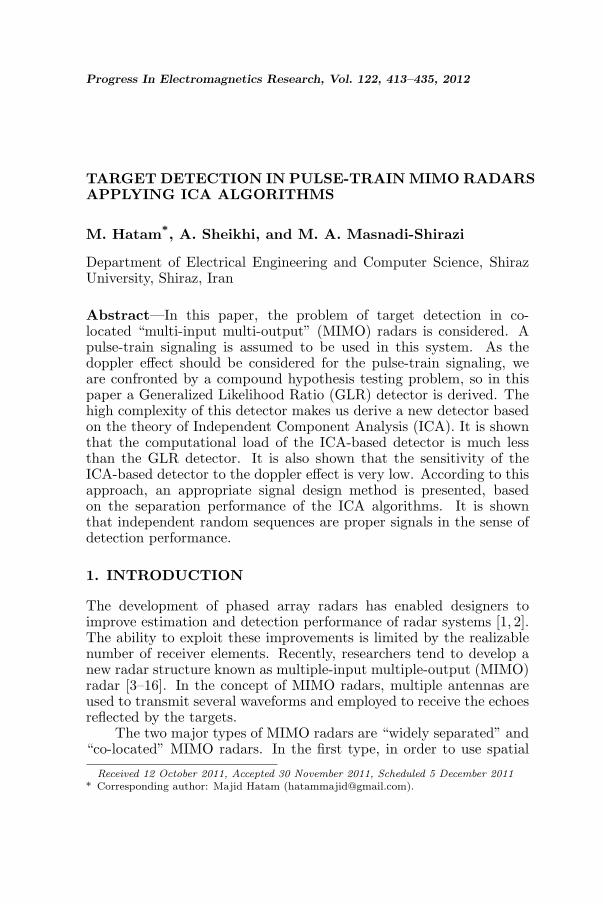
In [25], a pulse-train signaling for co-located MIMO radarshas been proposed. In the former techniques, an inter-pulse codemodulation has been employed (first row of Fig. 1). But in theproposed technique, a pulse-train signaling approach is utilized, andan intra-pulse code modulation is employed (second row of Fig. 1). In
Progress In Electromagnetics Research, Vol. 122, 2012 415
ci L1 cc
p : pulse withw
ic : i'th sample of
code sequence
pw = L τ p
c1 i Lcc
_+ + +_
_+
_
pw = τ p
Figure 1. Comparison of theinter-pulse and the intra-pulsecode modulations.
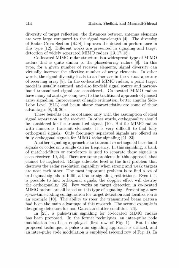
Figure 2. A uniform linear ar-ray by a set of m jointly transmit-ter/receiver antenna elements.
this approach, each radar transmitting element radiates a unique batchof pulses coded in phase and/or amplitude.
In the presented signaling, different carrier frequencies are usedin different transmitters. Applying the frequency difference of ∆f =1/τp to all m transmitters, the range resolution can be improved tocτp/2m according to the idea of “Stepped Frequency Radars” [27–29]. In the inter-pulse modulation signaling, the codes should bedesigned according to the criteria of good separability and properpulse compression property. But in the proposed signaling the codesshould be designed only based on the separability criterion and thepulse compression is achieved by the stepped frequency idea. So,the complexity of code design is decreased in the proposed signalingscheme.
In this paper, the problem of target detection in MIMO radarsusing this type of signaling is considered. The received signalmodeling and problem formulation are presented in Section 2. Itis shown that due to unknown values of doppler frequency andtarget DOA, a compound hypothesis testing problem is confronted.The standard technique for compound hypothesis tests when theProbability Distribution Function (PDF) of the unknown parametersare not known is the Generalized Likelihood Ratio (GLR) detection.
In Section 3, the GLR detector is derived. Except invarianceand asymptotic performance, there is no optimality claimed onGLR [30]. So, it is reasonable to investigate other detection strategies.
416 Hatam, Sheikhi, and Masnadi-Shirazi
In Section 4, the problem formulation is simplified and applyingIndependent Component Analysis (ICA) algorithms, an ICA-baseddetector is presented. A brief review on ICA techniques is alsooffered in this section. To achieve a good detection performance, theperformance of ICA techniques for separation of different transmittedsignals is considered as a constraint to design a set of codes for pulse-train signaling. This signal design technique is presented in Section 5.A brief analysis of computational complexity of two presented detectorsis offered in Section 6. Finally, in Section 7 simulation resultsare presented to evaluate the detection performance of the proposeddetectors.
2. PROBLEM FORMULATION
Without loss of generality, in this paper a co-located MIMO radarwith a Uniform Linear Array (ULA) is considered which is formed bya set of m jointly transmitting/receiving antenna elements separatedby 0.5λ (Fig. 2).† The pulse-train signaling proposed in [25] is used.Considering a fixed pulse width of τp and the Pulse Repetition Interval(PRI) of Tp, the narrow-band transmitted pulse trains are denoted bysk (t), k = 1, . . . , m:
{sk(t) 6= 0 q × Tp ≤ t ≤ q × Tp + τp
sk(t) = 0 else(1)
where q = 0, 1, 2, . . . , L and L is the number of transmitted pulsesfrom each transmitter. In this signaling, a single chip pulse withsuitable duration τp, according to the desired range resolution (cτp/2m)is transmitted during each Tp. In each transmitted pulse train, theamplitude and phase of signal can be changed in a suitable manner tomake all sk (t)s separable. It is assumed that the transmitted signalshave different carrier frequencies, with ∆f = 1/τp differences. If thecenter carrier frequency is denoted by fc, each transmitted signal has
a small frequency shift of ∆fk = (k − m + 12
) ×∆f related to fc. Sothe m × 1 vector of base-band received signal from a far-filled pointtarget, for each transmitted signal is given by:
xk(t) = αek(θ)bk(θ)sk(t− τ) exp (2πi (fdk+ ∆fk) t + i× kφ) (2)
where τ is the received signal delay and φ = −2π∆f × τ is the phaserelated to this delay. α is a complex constant, containing the effect† Here, we assume an equal number of transmitting and receiving elements. In our model,it is possible to have different numbers of them. But the number of receiving elementsshould be more than or at least equal to the number of transmitting elements.
Progress In Electromagnetics Research, Vol. 122, 2012 417
of power, RCS and propagation loss. For a single point target in thismodel, α is constant for all the transmitted signals, due to the co-located antenna assumption. e (θ) is the m×1 array factor of receivingantennas for the direction of target, bk (θ) is the kth transmitter factorand depends on the direction of target and fdk
is the target dopplerfrequency. Assuming radial velocity V , fdk
is given by:
fdk=
2V
λk=
2V
λ× λ
λk= fd × λ
λk(3)
where λk is the wavelength of kth transmitted signal and fd
is the doppler value, corresponding to λ that is the centerwavelength. Completely similar to the theory of “Stepped FrequencyRadars” [27, 28], the range dependent phase variation can be used toimprove the range resolution of this system. If we set ∆f = 1/τp, andif the delay is τ = n× τp + δτ , the phase would be φ = −2πn− 2π δτ
τp=
−2π δττp
. As we have only m samples to estimate φ, the resolution ofphase estimation is about 2π/m that is identical to the range resolutionof cτp/2m.
We define fk = (fdk+ ∆fk) for each transmitted signal and so we
can rewrite (2) as:
xk(t) = αek(θ)bk(θ)sk(t− τ) exp (2πifkt + i× kφ) (4)
The jth element of ek (θ) is given by:
{ek(θ)}j = exp{
2πidj
λksin(θ)
}j, k = 1, . . . , m (5)
Here, dj indicates the relative position of the jth receiving elementfrom the array center. Also, we can formulate the kth transmitterfactor bk (θ) as:
bk(θ) = exp{
2πidk
λksin(θ)
}k = 1, . . . ,m (6)
Considering n (t) as the vector of additive Gaussian noise ofreceiver elements, the vector of received signal (x (t)), would be:
x(t) =m∑
k=1
xk(t) + n(t)
=m∑
k=1
αek(θ)bk(θ) exp(i× kφ)sk(t− τ) exp(2πifkt) + n(t)
= α
m∑
k=1
ak(θ, φ)sk(t− τ) + n(t) = αA(θ, φ)s(t− τ) + n(t) (7)
418 Hatam, Sheikhi, and Masnadi-Shirazi
where the m×1 vector ak (θ, φ) which is the kth column of the m×mmixing matrix A (θ, φ), is given by:
{ak(θ, φ)}j = {ek(θ)}jbk(θ) exp(i× kφ) j = 1, . . . ,m (8)s (t−τ) is the m×1 vector of delayed and frequency shifted source
signals and we have:{s(t− τ)}k = sk(t− τ) exp(2πifkt) k = 1, . . . ,m (9)
In this model, the direction of target (θ), the exact value of φ and thedoppler value of signal (fd) are assumed to be unknown. Consideringthe pulse repetition interval of Tp, after range sampling of the receivedarray signal at times t = `×Tp+rτp for ` = 1, . . . , L and r = 1, . . . ,
Tp
τp,
we have R = Tp
τprange cells and we can form a m × L matrix of
received data for each range cell in which L denotes the number oftransmitted/received pulses. If τ = n× τp + δτ , for the nth range cell,we have:
Xm×L = αA(θ, φ)Sm×L + Nm×L = αm∑
k=1
ak(θ, φ)sTk + Nm×L (10)
where N contains the independent samples of receiver Gaussian noise.In this notation, (.)T denotes transpose and the L× 1 vector sk whichis the kth column of Sm×L, contains the samples of sk (t − τ) at thedesired delay for L consecutive pulses. Each element of sk can bewritten as:
{sk}` = {sk}` × exp(2πifk(`× Tp + nτp)) (11)where {sk}` = sk(`×Tp+δτ ). Now, we can form the detection problemas:
X = αA(θ, φ)S(fd) + N (12){H0 : α = 0H1 : α 6= 0
where θ, fd, φ and α are unknown parameters and so (12) is acompound hypothesis testing problem. In this paper, we assume thatall of the receiver noise vectors are N (0, σ2
nIm) where σ2n is known and
the noise vectors of different receiver elements are independent.When the PDFs of the unknown parameters are not known and
the Uniformly Most Powerful (UMP) detectors can not be found, thestandard technique for compound hypothesis tests would be the GLRdetector. There is no optimality claimed about GLR, except invarianceand asymptotic performance [30]. So, it is reasonable to investigateother detection strategies. In the next sections, different detectors forthis problem would be proposed.
Progress In Electromagnetics Research, Vol. 122, 2012 419
3. GLR DETECTOR
The GLR detector for the compound hypothesis test of (12) is:
fX
(X|H1, θ, α, φ, fd
)
fX (X|H0)≷ η (13)
where θ, α, φ and fd are the Maximum Likelihood (ML) estimationsof θ, α, φ and fd, respectively. This GLR detector is derived for thecompound hypothesis test of (12) in Appendix A and is given by:
maxfd,θ,φ
∣∣∣tr(A(θ, φ)S(fd)XH
)∣∣∣2
∥∥∥A(θ, φ)S(fd)∥∥∥
2 ≷ η (14)
In this notation, tr(·) denotes trace of matrix. It is determinedthat the GLR detector leads to a maximization over all realizable valuesof θ, φ and fd and also comparing this maximum with a threshold. Ifnf is the number of desired doppler values in the interval of [0, PRF),nφ is the number of phase test points and nθ is the number of directiontest points in the interval of [0, π], the complexity of this detector canbe justified with nf × nθ × nφ that requires a heavy processing power.The frequency space of doppler test point and also, the space betweendirection test point are very important in this method. But increasingthe number of doppler, phase and direction test points, would enhancethe computational complexity of GLR detection algorithm.
In the next section, it will be shown that considering thestatistical characteristics of transmitted pulse trains, the ML estimatedparameters used in the GLR detector can be replaced by ICA estimatedvalues of these parameters to form an ICA-based detector.
4. ICA-BASED DETECTOR
In pulse-train technique, we can change the amplitude and/or phaseof signal in a certain manner for each transmitter unit. Randomor pseudo-random pulse to pulse coding is a good example. Therandomness and independency of transmitted signals from pulse topulse, enable us to use ICA algorithms as a proper solution inestimation of unknown parameters. Therefore, instead of applyingML estimator in the structure of GLR detector, an ICA estimator canbe applied. So, we present the ICA-based detector as:
fX
(X|H1, θ, α, φ, fd
)
fX (X|H0)≷ η (15)
420 Hatam, Sheikhi, and Masnadi-Shirazi
where θ, α, φ and fd are the ICA estimations of θ, α, φ and fd.In Appendix B, it has been shown that the decisive rule of (15) isequivalent to:∣∣∣∣2Re
[tr
(αA(θ, φ)S(fd)XH
)]−
∥∥∥αA(θ, φ)S(fd)∥∥∥
2∣∣∣∣ ≷ η (16)
It should be noted that instead of θ, α, φ and fd, we only need toestimate αA (θ, φ) and S (fd). Before presenting the complete solutionof the ICA-based estimators, a brief review to ICA is offered in thenext subsection.
4.1. ICA Model
The theory of ICA, is totally described in [31–34]. In the standardICA model, we suppose a linear structure of the form:
X = AS +N (17)
when S is an m×L dimensional matrix of source signals. The rows ofS, named sT
k , k = 1, . . . , m are all independent and each sTk is a vector
of L i.i.d samples. A is the unknown m × m mixture matrix and Nis the additive Gaussian noise. Also, X is the available data matrix inwhich any row (xT
k ) is a linear mixture of independent source signals(sT
k ) contaminated with noise.Different ICA methods are all designed to estimate A or
equivalently W = A−1 and the source signals, S. Since A andS are both unknown, without assuming independent source signals,the problem cannot be solved in general. Different ICA methodsuse different available statistical properties of signals to solve thisestimation problem. ICA finds the desired sources by maximizing thestatistical independence of the estimated components. There are manyways to define independency and each way may result in a differentform of the ICA algorithm. The two major definitions for independencein ICA are based on “Minimization of Mutual Information” and“Maximization of non-Gaussianity”.
The family of ICA algorithms, based on maximization of non-Gaussianity, originate from the idea of central limit theorem. Higherorder statistics are proper tools to measure the non-Gaussianity ofsignals. JADE, introduced by Cardoso [35], is the most commonly usedmethod in this class. Because of the proper performance for separationof complex signals, in this paper we focus on using the complex formof the JADE algorithm [36].
ICA methods have two common restrictions. The first is thatthey cannot determine the power and phase of source signals and the
Progress In Electromagnetics Research, Vol. 122, 2012 421
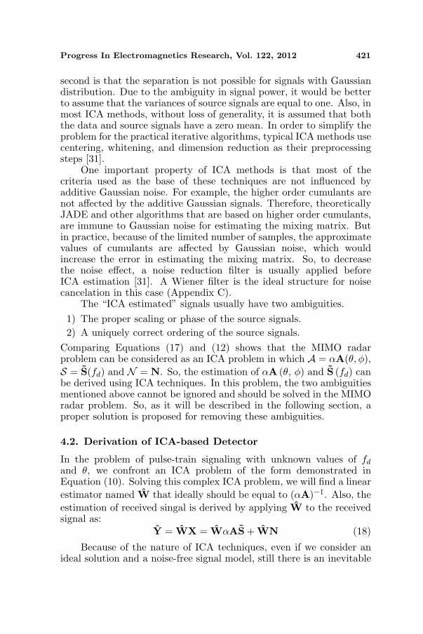
second is that the separation is not possible for signals with Gaussiandistribution. Due to the ambiguity in signal power, it would be betterto assume that the variances of source signals are equal to one. Also, inmost ICA methods, without loss of generality, it is assumed that boththe data and source signals have a zero mean. In order to simplify theproblem for the practical iterative algorithms, typical ICA methods usecentering, whitening, and dimension reduction as their preprocessingsteps [31].
One important property of ICA methods is that most of thecriteria used as the base of these techniques are not influenced byadditive Gaussian noise. For example, the higher order cumulants arenot affected by the additive Gaussian signals. Therefore, theoreticallyJADE and other algorithms that are based on higher order cumulants,are immune to Gaussian noise for estimating the mixing matrix. Butin practice, because of the limited number of samples, the approximatevalues of cumulants are affected by Gaussian noise, which wouldincrease the error in estimating the mixing matrix. So, to decreasethe noise effect, a noise reduction filter is usually applied beforeICA estimation [31]. A Wiener filter is the ideal structure for noisecancelation in this case (Appendix C).
The “ICA estimated” signals usually have two ambiguities.1) The proper scaling or phase of the source signals.2) A uniquely correct ordering of the source signals.
Comparing Equations (17) and (12) shows that the MIMO radarproblem can be considered as an ICA problem in which A = αA(θ, φ),S = S(fd) and N = N. So, the estimation of αA (θ, φ) and S (fd) canbe derived using ICA techniques. In this problem, the two ambiguitiesmentioned above cannot be ignored and should be solved in the MIMOradar problem. So, as it will be described in the following section, aproper solution is proposed for removing these ambiguities.
4.2. Derivation of ICA-based Detector
In the problem of pulse-train signaling with unknown values of fd
and θ, we confront an ICA problem of the form demonstrated inEquation (10). Solving this complex ICA problem, we will find a linearestimator named W that ideally should be equal to (αA)−1. Also, theestimation of received singal is derived by applying W to the receivedsignal as:
Y = WX = WαAS + WN (18)
Because of the nature of ICA techniques, even if we consider anideal solution and a noise-free signal model, still there is an inevitable
422 Hatam, Sheikhi, and Masnadi-Shirazi
ambiguity in the phase and order of signals that can be formulated as:
yk = exp(iϕk)× sj ξk = exp(−iϕk)× aj (19)
where the L× 1 vector yk is the kth estimated signal (kth row of Y)which does not normally correspond to the kth signal sk. Also, ξk
is the kth column of W−1 which is not necessarily equal to the kthcolumn of αA and ϕks are arbitrary phases. Now, in order to completethe estimation process, these ambiguities should be removed.
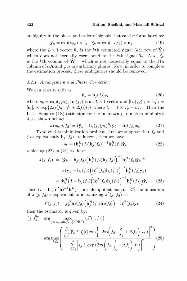
4.2.1. Arrangement and Phase Correction
We can rewrite (19) asyk = hj(fd)ρk (20)
where ρk = exp(jϕk), hj (fd) is an L× 1 vector and [hj(fd)]` = [sj ]` =[sj ]` × exp{2πi(fd · λ
λj+ ∆fj)t`} where t` = ` × Tp + nτp. Then the
Least-Squares (LS) estimator for the unknown parameters minimizesJ , as shown below:
J(ρk, j, fd) = (yk − hj(fd)ρk)H(yk − hj(fd)ρk) (21)
To solve this minimization problem, first we suppose that fd andj or equivalently hj (fd) are known, then we have:
ρk = (hHj (fd)hj(fd))−1hH
j (fd)yk (22)
replacing (22) in (21) we have
J(j, fd) = (yk − hj(fd)(hH
j (fd)hj(fd))−1
hHj (fd)yk)H
×(yk − hj(fd)(hH
j (fd)hj(fd))−1
hHj (fd)yk)
= yHk
(I − hj(fd)
(hH
j (fd)hj(fd))−1
hHj (fd)
)yk (23)
since (I − h (hHh)−1hH) is an idempotent matrix [37], minimizationof J (j, fd) is equivalent to maximizing J ′ (j, fd) as
J ′(j, fd) = yHk hj(fd)
(hH
j (fd)hj(fd))−1
hHj (fd)yk (24)
then the estimator is given by:
(j, fkd )=arg max
j=1,...,m,fd∈[0,PRF)
(J ′(j, fd)
)
=arg maxj,fd
∣∣∣∣n∑
`=1
yk[`]s∗j [`] exp{−2πi
(fd · λ
λj+ ∆fj
)·t`
}∣∣∣∣2
n∑`=1
∣∣∣∣sj [`] exp{2πi
(fd · λ
λj+∆fj
)·t`
}∣∣∣∣2
(25)
Progress In Electromagnetics Research, Vol. 122, 2012 423
Considering equal power for the transmitted signals, this estimatorcan be simplified as a windowed periodogram estimator as:
(j, fkd )=argmax
j,fd
(J ′(j, fd)
)
=arg maxj,fd
1
N
∣∣∣∣∣n∑
`=1
yk[`]s∗j [`] exp{−2πi
(fd · λ
λj+∆fj
)·t`
}∣∣∣∣∣2 (26)
Applying this estimator, the arrangement is complete. Accordingto (25), (26), the arrangement of signals can be performed with aweighted FFT in practice. After signal arrangement, the estimatedvector hj (fk
d ), should be applied to (22). So the phase estimator isgiven by:
ρk =(hj(f
kd )Hhj(f
kd )
)−1hj(f
kd )H yk (27)
where [hj(fkd )]` = [sj ]` × exp{2πi(fk
d · λ
λj
+ ∆fj)t`}. Applying
arrangement and phase correction, the estimated column of arraymatrix B = αA is obtained as:
bj = ˆαaj = ρ∗k · ξk (28)
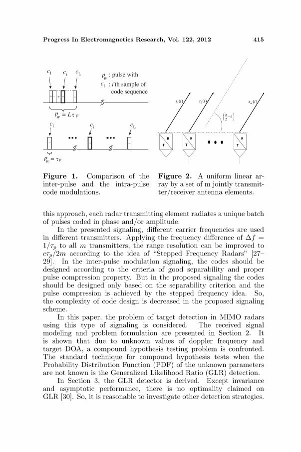
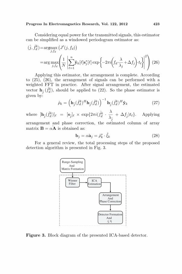
For a general review, the total processing steps of the proposeddetection algorithm is presented in Fig. 3.
Range-Sampling
AndMatrix Formation
WienerFilter
ICAEstimation
ArrangementAnd
Phase Correction
Detector Formation
Andη<>
Figure 3. Block diagram of the presented ICA-based detector.
424 Hatam, Sheikhi, and Masnadi-Shirazi
5. SIGNAL DESIGN
ICA is a powerful tool used to simplify our detection problem. In thispaper, we use ICA estimation technique to separate the mixture of “thesignal matrix” and “the array matrix”. In ICA techniques, informationabout mixed signals enables us to solve the estimation problem.Independency is the most important granted property, but otherparameters about signals such as probability density function(PDF)should be considered too. Now the question is, which signals arebetter separated in this model? In other words, the performance ofestimation with ICA should be evaluated by a quantitative parametersuch as variance of error or in a more general case, Cramer Rao Bound(CRB). This question is the basis for designing the transmitted pulsetrains.
As we completely described in [25] and as it was shownin [38, 39], the bounded magnitude signals such as BPSK and uniformlydistributed signals have better performance according to the CRB. So,in this paper we consider them for radar signal design as described inthe next subsection.
5.1. Code Sequence Design
In this paper, an ICA problem of the form demonstrated inEquation (10) is discussed. We can easily transform this time domainequation to an equivalent frequency domain by matrix multiplicationas:
Xf = X · F = AS · F + N · F = ASf + Nf (29)
where F is the L × L matrix of discrete Fourier transform, Xf is them × L matrix of the received signal in the frequency domain and Sf
contains the Fourier transform samples of S. In the time domain,the frequency shift of the signal may affect the estimated values ofthe covariance matrix, higher order statistics and other statisticalterms required in ICA estimation. Considering the doppler effect inthe frequency domain, it can be seen that the effect may cause onlya circular shift in the frequency samples of the signal. Therefore,the estimation of data statistics is more robust against the dopplervariation in the frequency domain. Therefore, the frequency domainmodeling of the signal as (29) leads to better results in ICA estimation.Solving this ICA problem, we will find the estimation of W = (αA)−1
named W.In the frequency domain, doppler effect causes only a circular
shift in the frequency samples, which does not change the statisticalcharacteristics of the data. This forces us to apply our ICA estimator
Progress In Electromagnetics Research, Vol. 122, 2012 425
RandomSignal
Generation
Mix with A (θ) fordifferent value of θ
1.
2. Apply ICA
3. Derive SIR
4. Select the best m × L
sequence
1
m
1 × L
1 × L
m × L
m × LInverse FFT
Transform
Transmitted
SequenceCode
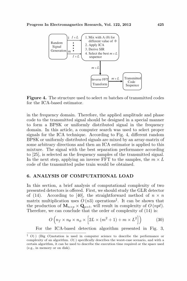
Figure 4. The structure used to select m batches of transmitted codesfor the ICA-based estimator.
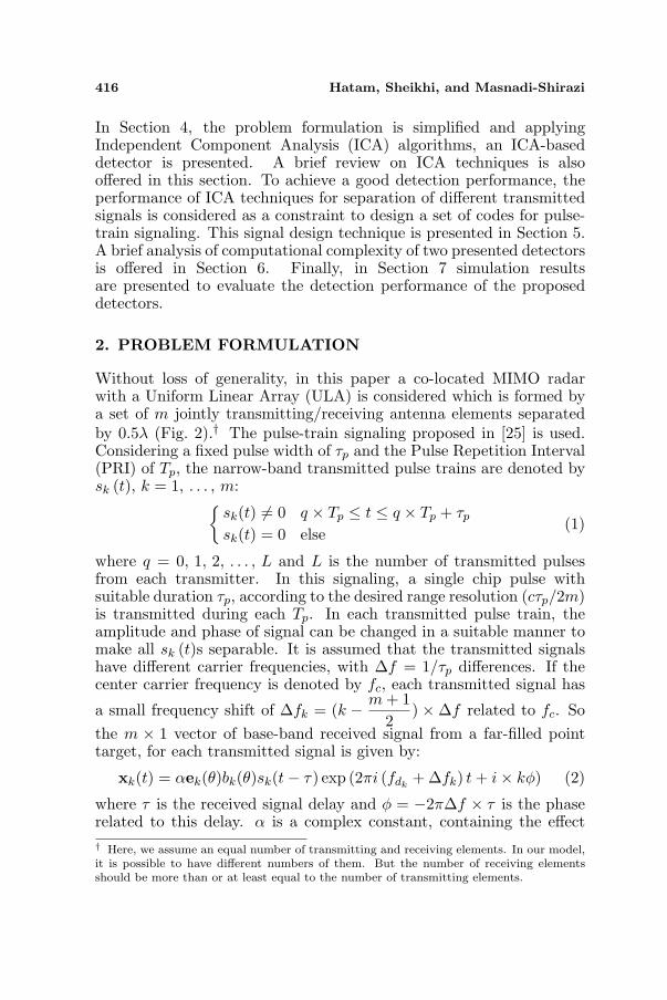
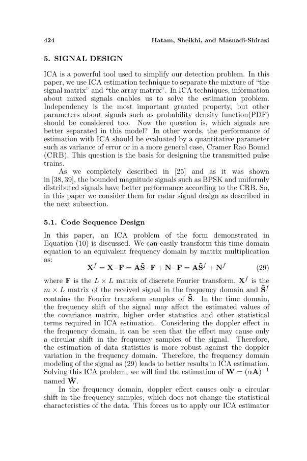
in the frequency domain. Therefore, the applied amplitude and phasecode to the transmitted signal should be designed in a special mannerto form a BPSK or uniformly distributed signal in the frequencydomain. In this article, a computer search was used to select propersignals for the ICA technique. According to Fig. 4, different randomBPSK or uniformly distributed signals are mixed by an array-matrix ofsome arbitrary directions and then an ICA estimator is applied to thismixture. The signal with the best separation performance accordingto [25], is selected as the frequency samples of the transmitted signal.In the next step, applying an inverse FFT to the samples, the m × Lcode of the transmitted pulse train would be obtained.
6. ANALYSIS OF COMPUTATIONAL LOAD
In this section, a brief analysis of computational complexity of twopresented detectors is offered. First, we should study the GLR detectorof (14). According to [40], the straightforward method of n × nmatrix multiplication uses O (n3) operations‡. It can be shown thatthe production of Mn×p ×Qp×`, will result in complexity of O (np`).Therefore, we can conclude that the order of complexity of (14) is:
O(nf × nθ × nφ ×
[2L× (m2 + 1) + m× L2
])(30)
For the ICA-based detection algorithm presented in Fig. 3,‡ O(·) (Big O)notation is used in computer science to describe the performance orcomplexity of an algorithm. O(·) specifically describes the worst-case scenario, and with acertain algorithm, it can be used to describe the execution time required or the space used(e.g., in memory or on disk).
426 Hatam, Sheikhi, and Masnadi-Shirazi
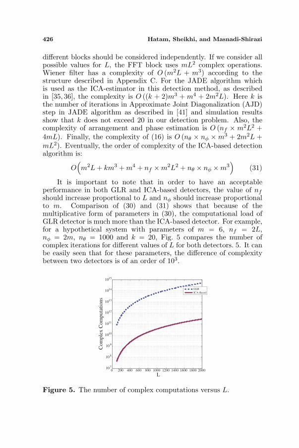
different blocks should be considered independently. If we consider allpossible values for L, the FFT block uses mL2 complex operations.Wiener filter has a complexity of O (m2L + m3) according to thestructure described in Appendix C. For the JADE algorithm whichis used as the ICA-estimator in this detection method, as describedin [35, 36], the complexity is O ((k + 2)m3 + m4 + 2m2L). Here k isthe number of iterations in Approximate Joint Diagonalization (AJD)step in JADE algorithm as described in [41] and simulation resultsshow that k does not exceed 20 in our detection problem. Also, thecomplexity of arrangement and phase estimation is O (nf × m2L2 +4mL). Finally, the complexity of (16) is O (nθ × nφ ×m3 + 2m2L +mL2). Eventually, the order of complexity of the ICA-based detectionalgorithm is:
O(m2L + km3 + m4 + nf ×m2L2 + nθ × nφ ×m3
)(31)
It is important to note that in order to have an acceptableperformance in both GLR and ICA-based detectors, the value of nf
should increase proportional to L and nφ should increase proportionalto m. Comparison of (30) and (31) shows that because of themultiplicative form of parameters in (30), the computational load ofGLR detector is much more than the ICA-based detector. For example,for a hypothetical system with parameters of m = 6, nf = 2L,nφ = 2m, nθ = 1000 and k = 20, Fig. 5 compares the number ofcomplex iterations for different values of L for both detectors. 5. It canbe easily seen that for these parameters, the difference of complexitybetween two detectors is of an order of 103.
0 200 400 600 800 1000 1200 1400 1600 1800 2000107
108
109
1010
1011
1012
1013
1014
1015
L
Co
mple
x C
om
puta
tio
ns
GLR
ICA-Based
Figure 5. The number of complex computations versus L.
Progress In Electromagnetics Research, Vol. 122, 2012 427
7. SIMULATION RESULTS
In this section, we consider a ULA array of omnidirectionaltransmit/receive antennas separated by 0.5λ. As described inSection 2, in the system presented here, a small shift is applied to thefrequency of different narrow-band transmitted signals. Considering acenter frequency of fc in these simulations, m transmitted frequenciesare uniformly spaced in an interval of fc±5%. In this section, an m = 6MIMO system with L = 200 is considered and the obtained sequencesaccording to Fig. 4 are used for simulation. Simulation results showthat in order to have equivalent performance with the case of knownφ (Loss ≤ 0.1 dB), we should select nφ ≥ 3m. So, nφ = 3m is used forthe simulations in this section.
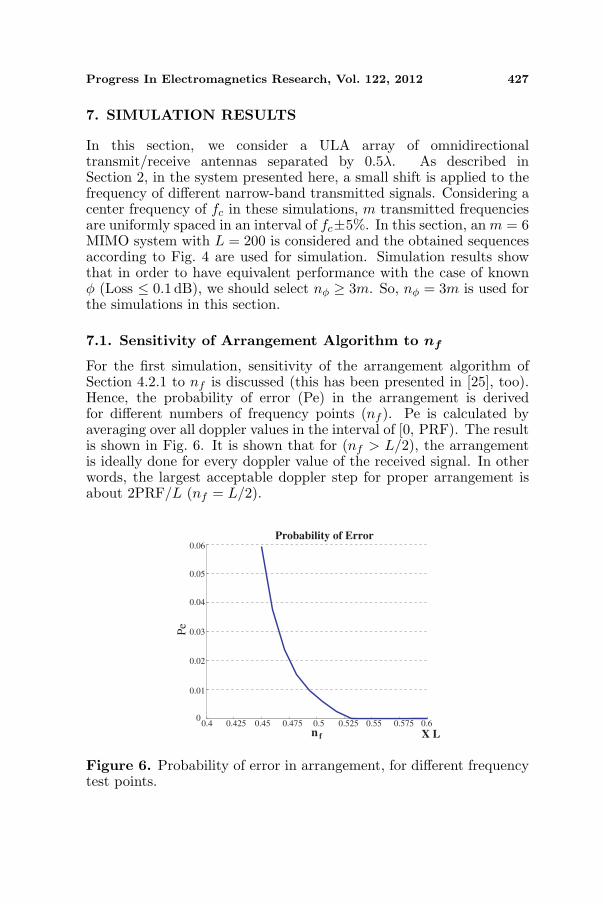
7.1. Sensitivity of Arrangement Algorithm to nf
For the first simulation, sensitivity of the arrangement algorithm ofSection 4.2.1 to nf is discussed (this has been presented in [25], too).Hence, the probability of error (Pe) in the arrangement is derivedfor different numbers of frequency points (nf ). Pe is calculated byaveraging over all doppler values in the interval of [0, PRF). The resultis shown in Fig. 6. It is shown that for (nf > L/2), the arrangementis ideally done for every doppler value of the received signal. In otherwords, the largest acceptable doppler step for proper arrangement isabout 2PRF/L (nf = L/2).
Probability of Error0.06
0.05
0.04
0.03
0.02
0.01
0
Pe
0.4 0.425 0.45 0.475 0.5 0.525 0.55 0.575 0.6
n f X L
Figure 6. Probability of error in arrangement, for different frequencytest points.
428 Hatam, Sheikhi, and Masnadi-Shirazi
7.2. Code Selection
As mentioned in Section 5.1, a computer search is used to select propertransmitted signals for the ICA-based detector. The procedure iscompletely described in Fig. 4. In this procedure, different sets ofuniformly distributed and random binary signals are applied. It isseen that ICA has a better performance in separation for the setsof uniformly distributed signals. So, in our simulations, this set ofm × L uniform signals (named c1) is utilized for ICA-based detector.A similar computer search is used for selecting a proper set of signals forGLR detector. In this procedure, different sets of uniform and randombinary signals are studied. The set with the highest probability ofdetection (Pd) is selected. It was found that the GLR detector is notso sensitive to the selected code. Therefore, in our simulations, a setof m× L uniform signals named c2 is utilized for the GLR detector.
7.3. Detection Performance
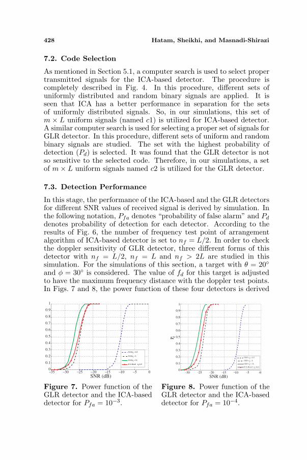
In this stage, the performance of the ICA-based and the GLR detectorsfor different SNR values of received signal is derived by simulation. Inthe following notation, Pfa denotes “probability of false alarm” and Pd
denotes probability of detection for each detector. According to theresults of Fig. 6, the number of frequency test point of arrangementalgorithm of ICA-based detector is set to nf = L/2. In order to checkthe doppler sensitivity of GLR detector, three different forms of thisdetector with nf = L/2, nf = L and nf > 2L are studied in thissimulation. For the simulations of this section, a target with θ = 20◦and φ = 30◦ is considered. The value of fd for this target is adjustedto have the maximum frequency distance with the doppler test points.In Figs. 7 and 8, the power function of these four detectors is derived
35 30 25 20 15 10 5 00
0.1
0.2
0.3
0.4
0.5
0.6
0.7
0.8
0.9
1
SNR (dB)
GLR nf = L/2
GLR nf = L
GLR nf > 2 L
ICA-Based nf=L/2
− − − − − − −
Figure 7. Power function of theGLR detector and the ICA-baseddetector for Pfa = 10−3.
30 25 20 15 10 5 00
0.1
0.2
0.3
0.4
0.5
0.6
0.7
0.8
0.9
1
SNR (dB)
P d
GLR nf = L/2
GLR nf = L
GLR nf > 2 L
ICA-Based nf=L/2
− − − − − − −
Figure 8. Power function of theGLR detector and the ICA-baseddetector for Pfa = 10−4.
Progress In Electromagnetics Research, Vol. 122, 2012 429
for Pfa = 10−3 and Pfa = 10−4. It is shown that in identical conditionof nf = L/2, the GLR detector has a very poor detection performancecompared to the ICA-based detector. Also, it can be seen that evenwith nf = L the performance of the GLR detector is weaker thanICA-based detector with nf = L/2. For example, for Pd = 0.9 andPfa = 10−3, the GLR detector with nf = L is about 0.2 dB weaker thanICA-based detector and this difference is even greater for lower valuesof Pd. This difference is about 0.4 dB for Pd = 0.9 and Pfa = 10−4.Figs. 7 and 8 show that unlike the ICA-based detector, the performanceof the GLR detector is very sensitive to nf . In this context, it is shownthat changing nf up to more than 2L improves the performance ofGLR detector about 2 dB.
8. CONCLUSION
The problem of target detection in a pulse-train co-located MIMOradar is investigated in this paper. Because of the unknown dopplervalue and unknown direction of target, we confront a compoundhypothesis testing problem, so, a GLR detector is derived in this paper.As the complexity of the GLR detector is very high, the practicalrealization of this detector is very difficult. So, a new detector based onthe theory of ICA algorithms is derived in this paper. In this context,a proper estimator is offered to rectify the phase and order ambiguityof ICA algorithms. A brief analysis of computational complexity ofthese two detectors is offered and it is shown that the computationalload of the ICA-based detector is much less than the GLR detector. Inaddition, simulation results show that the sensitivity of the ICA-baseddetector to the doppler effect is very low. Thus, with equal number ofdoppler test points, better detection performance is gained in the ICA-based detector. Finally, an appropriate signal design method basedon the separation performance of ICA algorithms is presented in thisresearch.
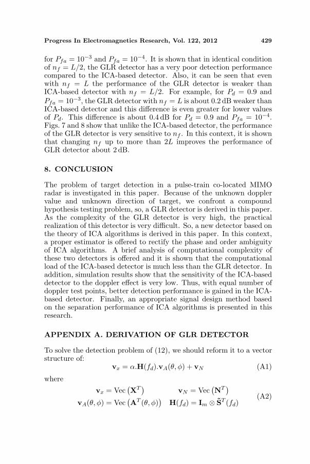
APPENDIX A. DERIVATION OF GLR DETECTOR
To solve the detection problem of (12), we should reform it to a vectorstructure of:
vx = α.H(fd).vA(θ, φ) + vN (A1)
where
vx = Vec(XT
)vN = Vec
(NT
)
vA(θ, φ) = Vec(AT (θ, φ)
)H(fd) = Im ⊗ ST (fd)
(A2)
430 Hatam, Sheikhi, and Masnadi-Shirazi
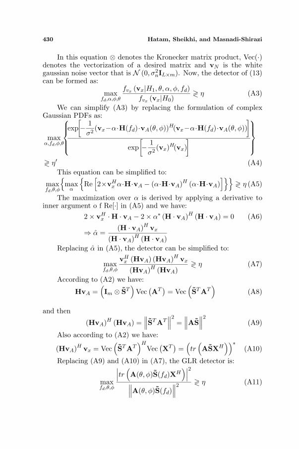
In this equation ⊗ denotes the Kronecker matrix product, Vec(·)denotes the vectorization of a desired matrix and vN is the whitegaussian noise vector that is N (0, σ2
nIL×m). Now, the detector of (13)can be formed as:
maxfd,α,φ,θ
fvx (vx|H1, θ, α, φ, fd)fvx (vx|H0)
≷ η (A3)
We can simplify (A3) by replacing the formulation of complexGaussian PDFs as:
maxα,fd,φ,θ
exp[− 1
σ2(vx−α·H(fd)·vA(θ, φ))H(vx−α·H(fd)·vA(θ, φ))
]
exp[− 1
σ2(vx)H(vx)
]
≷ η′ (A4)This equation can be simplified to:
maxfd,θ,φ
{max
α
{Re
[2×vH
x α·H·vA − (α·H·vA)H (α·H·vA)]}}
≷ η (A5)
The maximization over α is derived by applying a derivative toinner argument o f Re[·] in (A5) and we have:
2× vHx ·H · vA − 2× α∗ (H · vA)H (H · vA) = 0 (A6)
⇒ α =(H · vA)H vx
(H · vA)H (H · vA)Replacing α in (A5), the detector can be simplified to:
maxfd,θ,φ
vHx (HvA) (HvA)H vx
(HvA)H (HvA)≷ η (A7)
According to (A2) we have:
HvA =(Im ⊗ ST
)Vec
(AT
)= Vec
(STAT
)(A8)
and then
(HvA)H (HvA) =∥∥∥STAT
∥∥∥2
=∥∥∥AS
∥∥∥2
(A9)
Also according to (A2) we have:
(HvA)H vx = Vec(STAT
)HVec
(XT
)=
(tr
(ASXH
))∗(A10)
Replacing (A9) and (A10) in (A7), the GLR detector is:
maxfd,θ,φ
∣∣∣tr(A(θ, φ)S(fd)XH
)∣∣∣2
∥∥∥A(θ, φ)S(fd)∥∥∥
2 ≷ η (A11)
Progress In Electromagnetics Research, Vol. 122, 2012 431
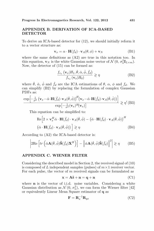
APPENDIX B. DERIVATION OF ICA-BASEDDETECTOR
To derive an ICA-based detector for (12), we should initially reform itto a vector structure as:
vx = α ·H(fd) · vA(θ, φ) + vN (B1)
where the same definitions as (A2) are true in this notation too. Inthis equation, vN is the white Gaussian noise vector of N (0, σ2
nIL×m).Now, the detector of (15) can be formed as:
fvx
(vx|H1, θ, α, φ, fd
)
fvx (vx|H0)≷ η (B2)
where θ, α, φ and fd are the ICA estimations of θ, α, φ and fd. Wecan simplify (B2) by replacing the formulation of complex GaussianPDFs as:
exp[− 1
σ2
(vx−α·H(fd)·vA(θ, φ)
)H(vx−α·H(fd)·vA(θ, φ)
)]
exp[− 1
σ2 (vx)H(vx)] ≷ η′ (B3)
This equation can be simplified to:
Re[2× vH
x α ·H(fd) · vA(θ, φ)− (α ·H(fd) · vA(θ, φ)
)H
(α ·H(fd) · vA(θ, φ)
) ]≷ η (B4)
According to (A2) the ICA-based detector is:∣∣∣∣2Re
[tr
(αA(θ, φ)S(fd)XH
)]−
∥∥∥αA(θ, φ)S(fd)∥∥∥
2∣∣∣∣ ≷ η (B5)
APPENDIX C. WIENER FILTER
Considering the described model in Section 2, the received signal of (10)is composed of L independent samples (pulses) of m×1 receiver vector.For each pulse, the vector of m received signals can be formulated as
x = As + n = q + n (C1)
where n is the vector of i.i.d. noise variables. Considering a whiteGaussian distribution as N (0, σ2
n), we can form the Wiener filter [42]or equivalently Linear Mean Square estimator of q as
F = R−1x Rqx (C2)
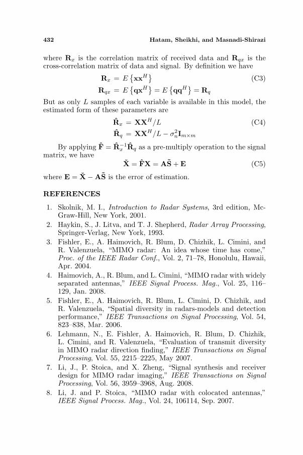
432 Hatam, Sheikhi, and Masnadi-Shirazi
where Rx is the correlation matrix of received data and Rqx is thecross-correlation matrix of data and signal. By definition we have
Rx = E{xxH
}(C3)
Rqx = E{qxH
}= E
{qqH
}= Rq
But as only L samples of each variable is available in this model, theestimated form of these parameters are
Rx = XXH/L (C4)
Rq = XXH/L− σ2nIm×m
By applying F = R−1x Rq as a pre-multiply operation to the signal
matrix, we haveX = FX = AS + E (C5)
where E = X−AS is the error of estimation.
REFERENCES
1. Skolnik, M. I., Introduction to Radar Systems, 3rd edition, Mc-Graw-Hill, New York, 2001.
2. Haykin, S., J. Litva, and T. J. Shepherd, Radar Array Processing,Springer-Verlag, New York, 1993.
3. Fishler, E., A. Haimovich, R. Blum, D. Chizhik, L. Cimini, andR. Valenzuela, “MIMO radar: An idea whose time has come,”Proc. of the IEEE Radar Conf., Vol. 2, 71–78, Honolulu, Hawaii,Apr. 2004.
4. Haimovich, A., R. Blum, and L. Cimini, “MIMO radar with widelyseparated antennas,” IEEE Signal Process. Mag., Vol. 25, 116–129, Jan. 2008.
5. Fishler, E., A. Haimovich, R. Blum, L. Cimini, D. Chizhik, andR. Valenzuela, “Spatial diversity in radars-models and detectionperformance,” IEEE Transactions on Signal Processing, Vol. 54,823–838, Mar. 2006.
6. Lehmann, N., E. Fishler, A. Haimovich, R. Blum, D. Chizhik,L. Cimini, and R. Valenzuela, “Evaluation of transmit diversityin MIMO radar direction finding,” IEEE Transactions on SignalProcessing, Vol. 55, 2215–2225, May 2007.
7. Li, J., P. Stoica, and X. Zheng, “Signal synthesis and receiverdesign for MIMO radar imaging,” IEEE Transactions on SignalProcessing, Vol. 56, 3959–3968, Aug. 2008.
8. Li, J. and P. Stoica, “MIMO radar with colocated antennas,”IEEE Signal Process. Mag., Vol. 24, 106114, Sep. 2007.
Progress In Electromagnetics Research, Vol. 122, 2012 433
9. Chen, C. Y. and P. Vaidyanathan, “MIMO radar space-timeadaptive processing using prolate spheroidal wave functions,”IEEE Transactions on Signal Processing, Vol. 56, 106–114,Sep. 2007.
10. Bekkerman, I. and J. Tabrikian, “Target detection andlocalization using MIMO radars and sonars,” IEEE Transactionson Signal Processing, Vol. 54, 3873–3883, Oct. 2006.
11. Daum, F. and J. Huang, “MIMO radar: Snake oil or good idea,”IEEE Aerosp. Electron. Syst. Mag., 8–12, May 2009.
12. Sheikhi, A. and A. Zamani, “Temporal coherent adaptive targetdetection for multi-input multi-output radars in clutter,” IETRadar, Sonar & Navig., Vol. 2, 86–96, Jun. 2008.
13. De Maio, A. and M. Lops, “Design principles of MIMO radardetectors,” IEEE Transactions on Aerospace and ElectronicSystems, Vol. 43, 886–897, Jul. 2007.
14. Huang, Y., P. Brennan, D. Patrick, I. Weller, P. Roberts, andK. Hughes, “FMCW based MIMO imaging radar for maritimenavigation,” Progress In Electromagnetics Research, Vol. 115,327–342, 2011.
15. Chen, J., Z. Li, and C. Li, “A novel strategy for topside ionospheresounder based on spaceborne MIMO radar with fdcd,” ProgressIn Electromagnetics Research, Vol. 116, 381–393, 2011.
16. Lim, S.-H., C. G. Hwang, S.-Y. Kim, and N.-H. Myung, “ShiftingMIMO SAR system for high-resolution wide-swath imaging,”Journal of Electromagnetic Waves and Applications, Vol. 25,No. 8–9, 1168–1178, 2011.
17. Yang, Y. and R. S. Blum, “Minimax robust MIMO radarwaveform design,” IEEE Journal of Sel. Topics Signal Process.,Vol. 1, 147–155, 2007.
18. Fuhrmann, D. and G. Antonio, “Transmit beamforming forMIMO radar systems using signal cross-correlation,” IEEE Trans.on Aerospace and Electronic Systems, Vol. 44, 171–176, Jan. 2008.
19. Qu, Y., G. Liao, S.-Q. Zhu, X.-Y. Liu, and H. Jiang,“Performance analysis of beamforming for MIMO radar,” ProgressIn Electromagnetics Research, Vol. 84 123–134, 2008.
20. Sinha, N. B., R. N. Bera, and M. Mitra, “Digital array MIMOradar and its performance analysis,” Progress In ElectromagneticsResearch C, Vol. 4, 25–41, 2008.
21. Hassanien, A. and S. A. Vorobyov, “Phased-MIMO radar:A tradeoff between phased-array and MIMO radars,” IEEETransactions on Signal Processing, Vol. 58, 3137–3151, Jun. 2010.
434 Hatam, Sheikhi, and Masnadi-Shirazi
22. Zhang, J., H. Wang, and X. Zhu, “Adaptive waveformdesign for separated transmit/receive ULA-MIMO radar,” IEEETransactions on Signal Processing, Vol. 58, 4936–4942, Sep. 2010.
23. Sen, S. and A. Nehorai, “OFDM MIMO radar with mutual-information waveform design for low-grazing angle tracking,”IEEE Transactions on Signal Processing, Vol. 58, 3152–3162,Jun. 2010.
24. Li, H. and B. Himed, “Transmit subaperturing for MIMO radarswith co-located antennas,” IEEE Journal of Selected Topics inSignal Processing, Vol. 4, 55–65, Feb. 2010.
25. Hatam, M., A. Sheikhi, and M. A. Masnadi-Shirazi, “A pulse-trainmimo radar based on theory of independent component analysis,”Submitted for Publication in the Iranian Journal of Science andTechnology, Jun. 2011.
26. Cui, G., L. Kong, and X. Yang, “Multiple-input multiple-outputradar detectors design in non-gaussian clutter,” IET Radar, Sonar& Navig., Vol. 4, 724–732, 2010.
27. Levenon, N., “Stepped-frequency pulse-train radar signal,” IEEProc. of Radar, Sonar and Navigation, Vol. 149, 297–309,Dec. 2002.
28. Iizuka, K., A. P. Freundorfer, et al., “Step-frequency radar,”Journal of Applied physics, Vol. 56, 2572–2583, Nov. 1984.
29. Mohseni, R., A. Sheikhi, and M. A. Masnadi-Shirazi, “Compres-sion of multicarrier phase-coded radar signals based on discretefourier transform (DFT),” Progress In Electromagnetics ResearchC, Vol. 5, 93–117, 2008.
30. Gabriel, J. R. and S. M. Kay, “On the relationship between theGLRT and UMPI tests for the detection of signals with unknownparameters,” IEEE Transactions on Signal Processing, Vol. 53,4194–4203, Nov. 2005.
31. Hyvarinen, A., J. Karhunen, and E. Oja, Independent ComponentAnalysis, John Wiley and Sons, New York, 2001.
32. Comon, P., “Independent components analysis: A new concept?,”Special Issue on Higher-order Statistics, Signal Processing,Elsevier, Vol. 36, 287–314, Apr. 1994.
33. Belouchrani, A., K. A. Meraim, J. F. Cardoso, and E. Moulines,“A blind source separation technique based on second orderstatistics,” IEEE Transactions on Signal Process, Vol. 45, 434–444, 1997.
34. Hyvarinen, A. and E. Oja, “A fast fixed-point algorithm forindependent component analysis,” IEEE Transactions on Neural

Progress In Electromagnetics Research, Vol. 122, 2012 435
Computations, Vol. 9, 1483–1492, Oct. 1997.35. Cardoso, J. F. and A. Souloumiac, “Blind beamforming for
non gaussian signals,” IEE Proceedings F, Radar and SignalProcessing, Vol. 140, 362–370, Dec. 1993.
36. Cardoso, J. F., “Jade algorithm for complex-valued signalsas a matlab function,” http://perso.telecom-paristech.fr/ car-doso/Algo/Jade/jade.m.
37. Kay, S. M., Fundamentals of Statistical Signal Processing:Estimation Theory, Vol. 1, Prentice-Hall, 1998.
38. Tichavsky, P., Z. Koldovsky, and E. Oja, “Performance analysisof the FastICA algorithm and Cramer-Rao bounds for linearindependent component analysis,” IEEE Transactions on SignalProcessing, Vol. 54, 1189–1203, Apr. 2006.
39. Koldovsky, Z., P. Tichavsky, and E. Oja, “Efficient variant ofalgorithm FastICA for independent component analysis attainingthe Cramr-Rao lower bound,” IEEE Transactions on NeuralNetworks, Vol. 17, 806–815, Sep. 2006.
40. Holtz, O. and N. Shomron, “Computational complexity andnumerical stability of linear problems,” Proceedings of the 5thEuropean Congress of Mathematics, 381–400, EMS PublishingHouse, 2010.
41. Todros, K. and J. Tabrikian, “Fast approximate joint diagonaliza-tion of positive definite hermitian matrices,” IEEE InternationalConference on Acoustics, Speech and Signal Processing, Vol. 3,2007.
42. Papoulis, A. and S. Pillai, Probability, Random Variables andStochastic Processes, 4th edition, Mc-Graw-Hill, 2002.