Taphonomic Trends Along a Forereef Slope: Lee Stocking Island, Bahamas. II. Time

66 RESEARCH REPORTS

Copyright Q 2002, SEPM (Society for Sedimentary Geology) 0883-1351/01/0017-066/$3.00

Taphonomic Trends Along a Forereef Slope: Lee StockingIsland, Bahamas. II. Time

GEORGE M. STAFFAustin Community College, NRG Campus, Geology Department 11928 Stonehollow Drive, Austin, TX 78758

W. RUSSELL CALLENDERNational Oceanic and Atmospheric Administration, Oceanic and Atmospheric Research, Office of Scientific Support,

1315 East-West Highway, Silver Spring, MD 20910

ERIC N. POWELLHaskin Shellfish Research Laboratory, Rutgers University, 6959 Miller Ave., Port Norris, NJ 08349

KARLA M. PARSONS-HUBBARDDepartment of Geology, Oberlin College, Oberlin, OH 44074

CARLTON E. BRETTDepartment of Geology, University of Cincinnati, Cincinnati, OH 45221

SALLY E. WALKERDepartment of Geology, University of Georgia, Athens, GA 30602

DONNA D. CARLSONDepartment of Geology, University of Cincinnati, Cincinnati, OH 45221

SUZANNE WHITEDepartment of Geology, University of Georgia, Athens, GA 30602

ANNE RAYMONDDepartment of Geology and Geophysics, Texas A&M University, College Station, TX 77843

ELIZABETH A. HEISEDepartment of Geology and Geophysics, Texas A&M University, College Station, TX 77843

PALAIOS, 2002, V. 17, p. 66–83

The Shelf and Slope Experimental Taphonomy Initiative(SSETI) Program was established to measure taphonomicrates in a range of continental shelf and slope environmentsover a long period of time. For this report, mollusk shellswere deployed for one and two years at seven different envi-ronments of deposition (EODs) along two onshore-offshoretransects off Lee Stocking Island in the Bahamas. The ex-perimental sites were located: in sand channels on the plat-form top (15 m) and the platform edge (33 m); on ledgesdown the wall (70–88 m); on the upper (183 m) and lower(210–226 m) talus slope below the wall; and on the crest(256–264 m) and in the trough (259–267 m) of large sanddunes. Shell condition was assessed using a range of taph-onomic attributes including dissolution, abrasion, edge al-teration, discoloration, and changes in shell weight.

After two years, taphonomic alteration was not particular-ly intense in any EOD. No species was particularly suscepti-ble or resistant to taphonomic alteration. Taphonomic pro-cesses were unexpectedly complex. Effects of location, tran-sect, water depth, and degree of exposure all had significanteffects. On average, shells deployed in shallow sites were al-

tered significantly from the controls more frequently thanshells deployed at deeper sites. However, the number of signif-icant interaction terms between time and the other main ef-fects indicates a complex interaction between taphonomicprocesses and the local environment that, over the short term,defies any attempt at delineating taphofacies over a broaderspatial area than a single deployment site. Some locations at-tained the same taphonomic signature in different waysmaking discrimination of taphonomic rules difficult. For ex-ample, deeper-water sites and shallow sites where burialrates were high yielded similar taphonomic signatures be-cause shells were in the aphotic zone in both cases, and thislimited the rate and range of taphonomic interactions. Taph-onomic processes were strongly nonlinear in time for alltaphonomic attributes in all species and all EODs. Nonlineartaphonomic rates hinder the interpretation of single-point-in-time studies in understanding the taphonomic processand buttress a commitment to long-term experiments.

INTRODUCTION

Understanding the importance of taphonomic bias isone of the necessities of paleoecological research. One of

BAHAMIAN TAPHONOMIC TRENDS: TIME 67

the central hypotheses of most taphonomic studies is thattaphonomic characteristics co-occur predictably, defining‘‘taphofacies’’ that can be used to characterize major envi-ronments of deposition. Furthermore, the spatial distri-bution of these taphofacies should be associated with en-vironmental gradients, such as depth and sediment type,that permit assemblage-level taphonomic signature to beinterpreted within the framework of preservation poten-tial and environment (Brett and Baird, 1986; Kidwell etal., 1986; Meldahl and Flessa, 1990; Speyer and Brett,1991; Callender et al., 1992; Kottler et al., 1992). Paleon-tologists apply to this effort a wealth of taphonomic infor-mation derived from actualistic studies documenting therelationship of the death assemblage and its preservation-al state to the living community. Powell et al. (1989), Par-sons and Brett (1991), Briggs (1995), Kidwell and Flessa(1995), and Kidwell (2001) summarize much of this infor-mation. A significant problem with the application of ac-tualistic data is that the present day is a work in progress.Most modern death assemblages are taphonomically ac-tive. Callender and Powell (1997) provide a comparison ofactive and inactive assemblages at petroleum seeps, as anexample. Meldahl et al. (1997) provides additional exam-ples from shallower water in the Gulf of California.

It is important to understand the rates of taphonomicprocesses so that the mechanisms underlying assemblageformation can be better understood and the inferences de-rived therefrom more safely applied to the fossil record.One approach is to follow the development of the death as-semblage from the living community (e.g., Cadee, 1968;Cummins et al., 1986; Staff et al., 1986). Under favorablecircumstances, cohorts can be followed through the livingcommunity into the death assemblage, and through theinitial phases of the preservational process. A second ap-proach is to evaluate taphonomic signature with respect tosome measure of time-since-death. This approach also canprovide estimates of the rates at which taphonomic pro-cesses proceed (Powell and Davies, 1990; Flessa et al.,1993; Meldahl et al., 1997; Moir, 1990). However, tapho-nomic rates are likely to be time-dependent. Many geo-chemical reactions are not of zero order (Boudreau, 1989;Middelburg, 1989; Berelson et al., 1990), for example, andthe application of the half-life concept to taphonomic de-struction of a cohort assumes a first-order process (Powellet al., 1984, 1986). Accordingly, an experimental approachis also necessary to understand the rates of taphonomicprocesses and how they change with time (Powell et al.,1989; Briggs, 1995).

Experimental taphonomic research has included labo-ratory-based approaches (Flessa and Brown, 1983; Gloverand Kidwell, 1993), field-based research (LaBarbera,1981, Tudhope and Risk, 1985; Walker, 1988; Walker andCarlton, 1995), or a combination of the two (Simon et al.,1994; Cutler, 1995). The majority of field-based studies inexperimental taphonomy have been restricted to near-shore regions generally shallower than 20 m because mosttaphonomic processes are extremely difficult to observebelow SCUBA depths. Notable exceptions include mea-surements of shell-fragment dissolution at hydrothermalvents (Killingley et al., 1980; Lutz et al., 1988, 1994), esti-mation of the rates of shell taphonomy at petroleum seeps(Callender et al., 1994), and biodegradation of skeletal ma-terial on shelves (Simon et al., 1994). Overall, develop-

ment of a theoretical framework for understanding taph-onomic processes has suffered from the high cost of work-ing in deeper shelf depths, the limitation in geographiccoverage of field deployments to a few EODs, and the lim-itation in time of deployment necessary to measure therates of taphonomic alteration in a way that would providetests of the taphofacies hypothesis.

The SSETI (Shelf and Slope Experimental TaphonomyInitiative) Program was established to measure tapho-nomic rates in a range of continental shelf and slope envi-ronments over a 10-year period. The SSETI Program is de-scribed in detail in Parsons et al. (1997) and Parsons-Hub-bard et al. (1999). Part of the SSETI program is located inthe Bahamas off Lee Stocking Island. Lee Stocking Islandis one of the many Exuma Islands and Cays that form theboundary between the eastern edge of the Great BahamasBank and the adjacent deep Exuma Sound (Kendall et al.,1990). The eastern side of Lee Stocking Island was select-ed because it has a steep reef wall that drops abruptlyfrom 33 m to depths exceeding 300 m; thus the site pro-vides an extensive depth gradient in a relatively smallgeographic area. The aim of this contribution is to describethe taphonomic alteration of a suite of molluscan shellsthat were deployed for one and two years along two tran-sects over a depth range of 15 to 267 m.

METHODS

Site Description

Experiments were deployed in 1993 and 1994 by SCU-BA and the submersible Nekton Gamma along transectsAA and BA established by the Caribbean Marine Re-search Center/National Undersea Research Program. Fig-ure 1 in Callender et al. (2002) identifies the location ofthese two transects. Transect AA is located directly off aninlet that separates Lee Stocking Island from Adderly Cayto the NNW. The shallow sites on the AA transect are sub-ject to fairly high wave-and-current energy and sedimenttransport due to close proximity to this inlet. Transect BAis SW of AA about half way down Lee Stocking Island and,as a consequence, is less impacted by current energy andsediment transport.

The individual experimental sites are located in sevendistinctive EODs along each transect (Fig. 1, Callender etal., 2002): in sand channels on the platform top (15 m) andthe platform edge (33 m), on ledges down the wall (70–88m), on the upper (183 m—transect BA only) and lower(210–226 m) talus slope below the wall, and on the crest(256–264 m) and in the trough (259–267 m) of large sanddunes. These deployment EODs will be referred to as lo-cations hereafter. Each location was represented by onesite on each transect, with the exception of the upper talusslope that was occupied only on transect BA. Thus, the ex-perimental design consisted of two transects and seven lo-cations, or thirteen total deployment sites. Parsons et al.(1997) and Parsons-Hubbard et al. (1999) provide descrip-tions of these sites, which are reviewed here and summa-rized in Table 1 of Callender et al. (2002).

The platform on the eastern edge of Lee Stocking Islandis characterized by a reef terrace containing carbonatesand flats, hardgrounds, and patch reefs that graduallydeepen from shore to the platform edge at about 33 m. Ex-

68 STAFF ET AL.

periments were placed in sand channels about midwayacross the platform top at 15 m and at its edge at 33 m.The 15-m experiments had moved significantly each year,probably coincident with large-scale sand transport thatwas documented by year-to-year changes in sediment cov-er. The experiments at 33 m were buried within the firstyear after deployment on both transects and not subse-quently re-exposed (as far as observations permit). Par-sons-Hubbard et al. (1999) provide details of the effect ofburial at these sites.

The slope steepens dramatically at the platform edgeand forms a wall that drops steeply (.608) into ExumaSound. The wall is punctuated by elongate narrow ledgesupon which the experimental arrays were positioned.These ledges have a thin veneer of coral-Halimeda-mol-luscan sand over a lithified surface and are subject to oc-casional periods of high current flow. Experiments weremoved over the two-year period, to some extent, on bothledges on transect AA, but on neither ledge on transectBA.

The photic zone extends to approximately the base ofthe wall. Below this point, at about 180 m, the forereefslope begins to moderate. This area is characterized byshingled carbonate debris, large talus blocks, and smalllithified carbonate outcrops separated by areas covered bya thin veneer (2–3 cm) of unconsolidated sediment.Stalked crinoids are observed frequently on the carbonateoutcrops, particularly on transect AA. Experiments wereplaced in the upper (shallower) and lower (deeper) halvesof the talus region. Downslope of the talus zone is a field oflarge partially-cemented dunes, each crest rising up to 10m above the adjacent trough. The dune crests roughly par-allel the reef wall, with each dune crest being deeper thanthe preceding one. Experiments were placed on the crestand in the trough of the first dune line downslope of the ta-lus field on each transect.

Experimental Design

The SSETI experimental design is described in detail inParsons et al. (1997) and summarized briefly here. Eachexperiment consisted of a series of 1-cm-mesh bags at-tached to a 1.5-m PVC pole. To each pole was attached a12-kg weight to counter a 25-cm square float made of 6-mm-thick sheet polypropylene. The float rose about 0.5 mabove the array and served to mark the location of the ex-periment even when buried. The PVC pole was unat-tached to the bottom, anchored only by the 12-kg weightand, hence, was free to move, given sufficient current andwave action. Experiments were moved at all 15-m sitesand even at some deployment sites as deep as 260 m (Ta-ble 1 in Callender et al., 2002), but the polypropylene floatpermitted the experiments to be relocated in every case.

Two of the mesh bags on each pole contained molluscanshells, typically five individuals of five different species,each separated from the others by plastic cable ties. Mol-luscan species deployed included the ocean quahog Arcticaislandica, the blue mussel Mytilus edulis, the lucinid Co-dakia orbicularis, the venerid Mercenaria mercenaria, theglycymerid Glycymeris undata, the cerithiids Telescopiumtelescopium and Rhinoclavus vertagus, and the conchStrombus luhuanus. The number of individuals of eachspecies recovered and analyzed after 1 and 2 years of de-

ployment time can be found in Table 2 of Callender et al.(2002).

Experiments were deployed on transect AA in 1993; oneset was recovered in 1994 and another in 1995 using theNekton Gamma. Experiments were deployed on transectBA in 1994; one set was recovered in 1995 and another in1996 using the submersibles Nekton Gamma and Clelia.In addition, at each site, loose bivalve and gastropod shellswere scattered freely on the sediment surface to furthermeasure rates of shell movement and burial. Parsons-Hubbard et al. (1999, 2001) analyzed the results of theseloose-shell deployments for 1 and 2 years of deploymenttime and characterized each shell deployment as exposed,dusted (by a fine layer of sediment), or buried after oneand two years.

Laboratory Analyses

Laboratory analyses of shell specimens commencedsoon after recovery and were completed within 48 hr. Dur-ing this time, shells were maintained in chilled seawateruntil analysis. Each shell was photographed, measured,assessed for taphonomic alteration, air-dried, andweighed. The types of taphonomic alteration assessed in-clude breakage, edge rounding, periostracum condition,discoloration from the original condition, and evidenceand severity of dissolution, abrasion, and authigenic pre-cipitation. Each of these was evaluated using a semi-quan-titative scale described by Davies et al. (1990) on each ofeight standard shell areas for bivalves on the inner andouter surfaces (see Davies et al., 1990) and on five stan-dard shell areas for gastropods somewhat modified fromDavies et al. (1990), specifically the spire aperture up,spire aperture down, body whorl aperture up, body whorlaperture down, and the inside aperture/columella com-plex.

For statistical analysis, taphonomic attributes weretreated in one of two ways. For dissolution, each shell areawas assigned a numerical value according to the degree ofdissolution. The semi-quantitative scale, simplified fromDavies et al. (1990), is defined in table 3 of Callender et al.(2002). To obtain the average condition for a shell, theweighted values for each shell area were averaged. Theweighting used was proportional to the fraction of the totalshell surface area contributed by that shell area. For theremaining taphonomic attributes, and as an alternativeway to evaluate dissolution, the most altered state ob-served on any of the discrete shell areas was taken as thevalue for that shell. In this case, the analysis focused onthe most extreme condition achieved on the shell. Thismethod of evaluation follows the approach used by Staffand Powell (1990), Callender and Powell (1992), and Cal-lender et al. (1994).

The change in shell condition over time was assessed inthree ways. First, the proportion of sites was tallied thatyielded shells with a taphonomic signature after one andtwo years that differed significantly (Mann-Whitney test,a 5 0.05) from controls that had remained on a laboratoryshelf. Second, the influence of time was assessed as anANOVA main effect, and as it interacted with transect-and-location main effects and with depth and exposure.These statistical analyses are further discussed in Callen-der et al. (2002). Third, a qualitative evaluation of the


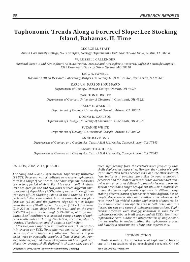
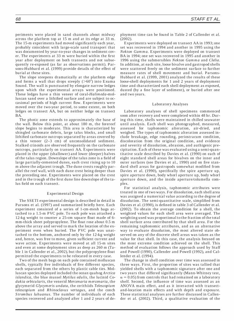
FIGURE 1—The proportion of statistical tests yielding a significantdifference between control and experimental arrays in Years 1 and 2for the eight species. Each set of deployed individuals for each spe-cies was tested against its control. Significance was judged at the a5 0.05 level. Test results were summed across all taphonomic attri-butes, transects, and locations for presentation. P-values given belowpresent the results of binomial tests designed to determine if the num-ber of significant differences in tests between control and experimentalgroups is greater than would be expected by chance at a 5 0.05.

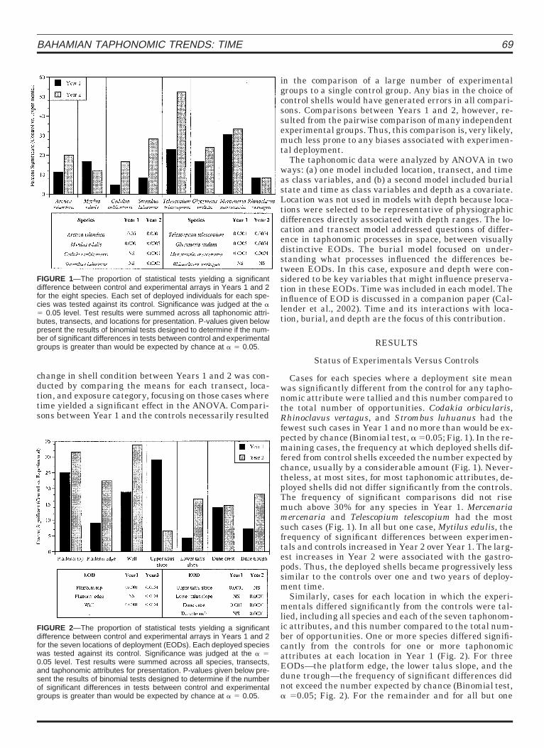
FIGURE 2—The proportion of statistical tests yielding a significantdifference between control and experimental arrays in Years 1 and 2for the seven locations of deployment (EODs). Each deployed specieswas tested against its control. Significance was judged at the a 50.05 level. Test results were summed across all species, transects,and taphonomic attributes for presentation. P-values given below pre-sent the results of binomial tests designed to determine if the numberof significant differences in tests between control and experimentalgroups is greater than would be expected by chance at a 5 0.05.

change in shell condition between Years 1 and 2 was con-ducted by comparing the means for each transect, loca-tion, and exposure category, focusing on those cases wheretime yielded a significant effect in the ANOVA. Compari-sons between Year 1 and the controls necessarily resulted

in the comparison of a large number of experimentalgroups to a single control group. Any bias in the choice ofcontrol shells would have generated errors in all compari-sons. Comparisons between Years 1 and 2, however, re-sulted from the pairwise comparison of many independentexperimental groups. Thus, this comparison is, very likely,much less prone to any biases associated with experimen-tal deployment.

The taphonomic data were analyzed by ANOVA in twoways: (a) one model included location, transect, and timeas class variables, and (b) a second model included burialstate and time as class variables and depth as a covariate.Location was not used in models with depth because loca-tions were selected to be representative of physiographicdifferences directly associated with depth ranges. The lo-cation and transect model addressed questions of differ-ence in taphonomic processes in space, between visuallydistinctive EODs. The burial model focused on under-standing what processes influenced the differences be-tween EODs. In this case, exposure and depth were con-sidered to be key variables that might influence preserva-tion in these EODs. Time was included in each model. Theinfluence of EOD is discussed in a companion paper (Cal-lender et al., 2002). Time and its interactions with loca-tion, burial, and depth are the focus of this contribution.

RESULTS

Status of Experimentals Versus Controls

Cases for each species where a deployment site meanwas significantly different from the control for any tapho-nomic attribute were tallied and this number compared tothe total number of opportunities. Codakia orbicularis,Rhinoclavus vertagus, and Strombus luhuanus had thefewest such cases in Year 1 and no more than would be ex-pected by chance (Binomial test, a 50.05; Fig. 1). In the re-maining cases, the frequency at which deployed shells dif-fered from control shells exceeded the number expected bychance, usually by a considerable amount (Fig. 1). Never-theless, at most sites, for most taphonomic attributes, de-ployed shells did not differ significantly from the controls.The frequency of significant comparisons did not risemuch above 30% for any species in Year 1. Mercenariamercenaria and Telescopium telescopium had the mostsuch cases (Fig. 1). In all but one case, Mytilus edulis, thefrequency of significant differences between experimen-tals and controls increased in Year 2 over Year 1. The larg-est increases in Year 2 were associated with the gastro-pods. Thus, the deployed shells became progressively lesssimilar to the controls over one and two years of deploy-ment time.

Similarly, cases for each location in which the experi-mentals differed significantly from the controls were tal-lied, including all species and each of the seven taphonom-ic attributes, and this number compared to the total num-ber of opportunities. One or more species differed signifi-cantly from the controls for one or more taphonomicattributes at each location in Year 1 (Fig. 2). For threeEODs—the platform edge, the lower talus slope, and thedune trough—the frequency of significant differences didnot exceed the number expected by chance (Binomial test,a 50.05; Fig. 2). For the remainder and for all but one

70 STAFF ET AL.

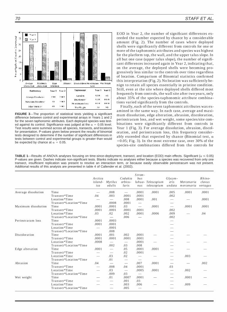
FIGURE 3—The proportion of statistical tests yielding a significantdifference between control and experimental arrays in Years 1 and 2for the seven taphonomic attributes. Each deployed species was test-ed against its control. Significance was judged at the a 5 0.05 level.Test results were summed across all species, transects, and locationsfor presentation. P-values given below present the results of binomialtests designed to determine if the number of significant differences intests between control and experimental groups is greater than wouldbe expected by chance at a 5 0.05.

TABLE 1—Results of ANOVA analyses focusing on time-since-deployment, transect, and location (EOD) main effects. Significant (a # 0.05)P-values are given. Dashes indicate non-significant tests. Blanks indicate no analyses either because a species was recovered from only onetransect, insufficient replication was present to resolve an interaction term, or because easily observable periostracum was not present.Additional results of this analysis are presented in table 4 of Callender et al. (2002).

Arcticaisland-

icaMytilusedulis

Codakiaorbicu-laris

Strom-bus

luhua-nus

Telescopiumtelescopium

Glycym-eris

undataMercenariamercenaria

Rhino-clavus

vertagus

Average dissolution TimeTransect*TimeLocation*TimeTransect*Location*Time

—.04

—

.008

.003—

.0008

—.0001.008.0001

.0001

.0001

.0001—

.0001

.001

.005

.002——

.0001

—

.0001

.0001

Maximum dissolution TimeTransect*TimeLocation*TimeTransect*Location*Time

.0001

.0001

.03

.0001

.0001

.02—

.03

.0001

.002

.006

—.0001.0001

—

.0001

.0006

—.002.009.002

.0001

—

.0001

.04

Periostracum loss TimeTransect*TimeLocation*TimeTransect*Location*Time

.0001

.0001—

.0003

.0001

.0001

.008

————

Discoloration TimeTransect*TimeLocation*TimeTransect*Location*Time

.0001

.0001

.0008

.001

.0001—

.002

.002

.0001—

.03

.0001

.0001

.0001

.008

—

—

————

—

—

—

—

Edge alteration TimeTransect*TimeLocation*TimeTransect*Location*Time

.0001——

——

.03

.01

.05

.02

.02—

.0001

.0001——

.0001

—

————

—

.003

—

—

Abrasion TimeTransect*TimeLocation*TimeTransect*Location*Time

.04——

—.008.03.009

—.04—

.03

.007

.0001

.0005—

.0001

.0001

—.03——

—

.002

.002

—

Wet weight TimeTransect*TimeLocation*TimeTransect*Location*Time

———

.01———

.0007

.001

.003

.005

.0001

.03

.006—

—

—

————

.0001

.009

—

—

EOD in Year 2, the number of significant differences ex-ceeded the number expected by chance by a considerableamount (Fig. 2). The number of cases where deployedshells were significantly different from controls for one ormore of the taphonomic attributes and species was highestfor the platform top, the wall, and the upper talus slope. Inall but one case (upper talus slope), the number of signifi-cant differences increased again in Year 2, indicating that,on the average, the deployed shells were becoming pro-gressively less similar to the controls over time regardlessof location. Comparison of Binomial statistics confirmedthis interpretation (Fig. 2). No location was sufficiently be-nign to retain all species essentially in pristine condition.Still, even at the site where deployed shells differed mostfrequently from controls, the wall site after two years, onlyabout 35% of the species-taphonomic attribute combina-tions varied significantly from the controls.

Finally, each of the seven taphonomic attributes was ex-amined in the same way. In each case, average and maxi-mum dissolution, edge alteration, abrasion, discoloration,periostracum loss, and wet weight, some species/site com-binations were significantly different from controls inYear 1 (Fig. 3). For average dissolution, abrasion, discol-oration, and periostracum loss, this frequency consider-ably exceeded that expected by chance (Binomial test, a50.05; Fig. 3). In the most extreme case, over 30% of thespecies-site combinations differed from the controls for


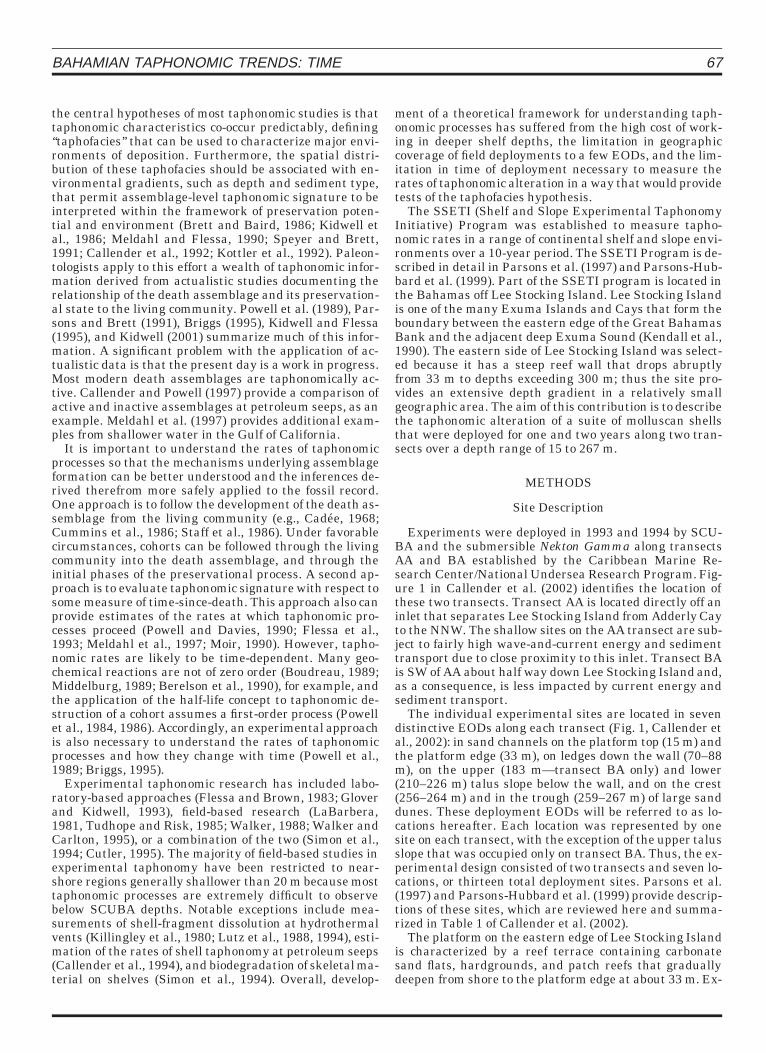
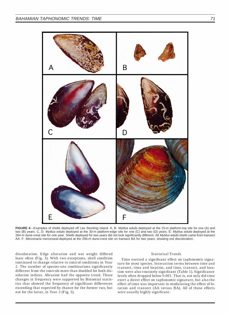
FIGURE 4—Examples of shells deployed off Lee Stocking Island. A, B: Mytilus edulis deployed at the 15-m platform-top site for one (A) andtwo (B) years. C, D: Mytilus edulis deployed at the 30-m platform-edge site for one (C) and two (D) years. E: Mytilus edulis deployed at the264-m dune-crest site for one year. Shells deployed for two years did not look significantly different. All Mytilus edulis shells came from transectAA. F: Mercenaria mercenaria deployed at the 256-m dune-crest site on transect BA for two years, showing red discoloration.

discoloration. Edge alteration and wet weight differedleast often (Fig. 3). With two exceptions, shell conditioncontinued to change relative to control conditions in Year2. The number of species-site combinations significantlydifferent from the controls more than doubled for both dis-solution indices. Abrasion had the opposite trend. Thesechanges in frequency were supported by Binomial statis-tics that showed the frequency of significant differencesexceeding that expected by chance for the former two, butnot for the latter, in Year 2 (Fig. 3).

Statistical TrendsTime exerted a significant effect on taphonomic signa-

ture for most species. Interaction terms between time andtransect, time and location, and time, transect, and loca-tion were also routinely significant (Table 1). Significancelevels often dropped below 0.001. That is, not only did timeexert a direct effect on taphonomic signature, but also theeffect of time was important in modulating the effect of lo-cation and transect (AA versus BA). All of these effectswere usually highly significant.

72 STAFF ET AL.

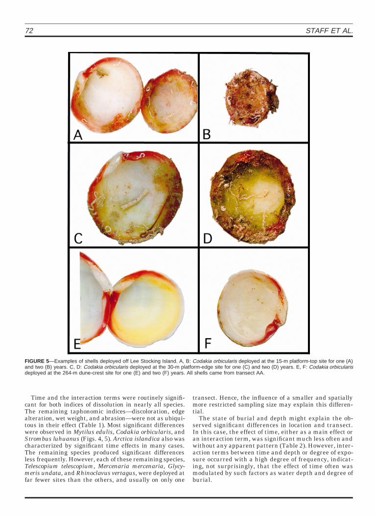
FIGURE 5—Examples of shells deployed off Lee Stocking Island. A, B: Codakia orbicularis deployed at the 15-m platform-top site for one (A)and two (B) years. C, D: Codakia orbicularis deployed at the 30-m platform-edge site for one (C) and two (D) years. E, F: Codakia orbicularisdeployed at the 264-m dune-crest site for one (E) and two (F) years. All shells came from transect AA.

Time and the interaction terms were routinely signifi-cant for both indices of dissolution in nearly all species.The remaining taphonomic indices—discoloration, edgealteration, wet weight, and abrasion—were not as ubiqui-tous in their effect (Table 1). Most significant differenceswere observed in Mytilus edulis, Codakia orbicularis, andStrombus luhuanus (Figs. 4, 5). Arctica islandica also wascharacterized by significant time effects in many cases.The remaining species produced significant differencesless frequently. However, each of these remaining species,Telescopium telescopium, Mercenaria mercenaria, Glycy-meris undata, and Rhinoclavus vertagus, were deployed atfar fewer sites than the others, and usually on only one

transect. Hence, the influence of a smaller and spatiallymore restricted sampling size may explain this differen-tial.

The state of burial and depth might explain the ob-served significant differences in location and transect.In this case, the effect of time, either as a main effect oran interaction term, was significant much less often andwithout any apparent pattern (Table 2). However, inter-action terms between time and depth or degree of expo-sure occurred with a high degree of frequency, indicat-ing, not surprisingly, that the effect of time often wasmodulated by such factors as water depth and degree ofburial.


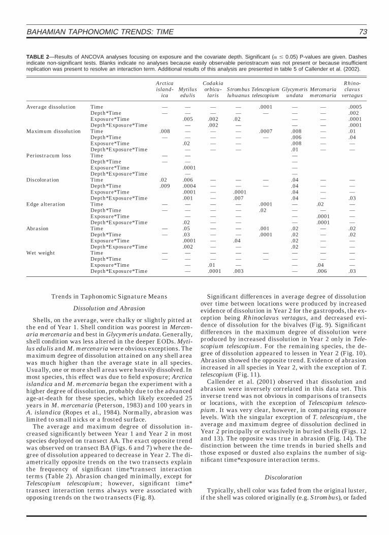
TABLE 2—Results of ANCOVA analyses focusing on exposure and the covariate depth. Significant (a # 0.05) P-values are given. Dashesindicate non-significant tests. Blanks indicate no analyses because easily observable periostracum was not present or because insufficientreplication was present to resolve an interaction term. Additional results of this analysis are presented in table 5 of Callender et al. (2002).

Arcticaisland-

icaMytilusedulis

Codakiaorbicu-laris

Strombusluhuanus

Telescopiumtelescopium

Glycymerisundata

Mercenariamercenaria

Rhino-clavus

vertagus

Average dissolution TimeDepth*TimeExposure*TimeDepth*Exposure*Time

——

——

.005—

——

.002

.002

——

.02—

.0001—

————

————

.0005

.002

.0001

.0001Maximum dissolution Time

Depth*TimeExposure*TimeDepth*Exposure*Time

.008—

——

.02—

————

————

.0007—

.008

.006

.008

.01

————

.01

.04——

Periostracum loss TimeDepth*TimeExposure*TimeDepth*Exposure*Time

——

——

.0001—

————

Discoloration TimeDepth*TimeExposure*TimeDepth*Exposure*Time

.02

.009.006.0004.0001.001

————

——

.0001

.007

——

.04

.04

.04

.04

————

———.03

Edge alteration TimeDepth*TimeExposure*TimeDepth*Exposure*Time

——

———

.02

————

————

.0001

.02————

.02—

.0001

.0001

————

Abrasion TimeDepth*TimeExposure*TimeDepth*Exposure*Time

——

.05

.03

.0001

.002

————

——

.04—

.001

.0001.02.02.02.02

————

.02

.02——

Wet weight TimeDepth*TimeExposure*TimeDepth*Exposure*Time

——

————

——

.01

.0001

———

.003

——

————

——

.04

.006

———.03

Trends in Taphonomic Signature Means

Dissolution and Abrasion

Shells, on the average, were chalky or slightly pitted atthe end of Year 1. Shell condition was poorest in Mercen-aria mercenaria and best in Glycymeris undata. Generally,shell condition was less altered in the deeper EODs. Myti-lus edulis and M. mercenaria were obvious exceptions. Themaximum degree of dissolution attained on any shell areawas much higher than the average state in all species.Usually, one or more shell areas were heavily dissolved. Inmost species, this effect was due to field exposure; Arcticaislandica and M. mercenaria began the experiment with ahigher degree of dissolution, probably due to the advancedage-at-death for these species, which likely exceeded 25years in M. mercenaria (Peterson, 1983) and 100 years inA. islandica (Ropes et al., 1984). Normally, abrasion waslimited to small nicks or a frosted surface.

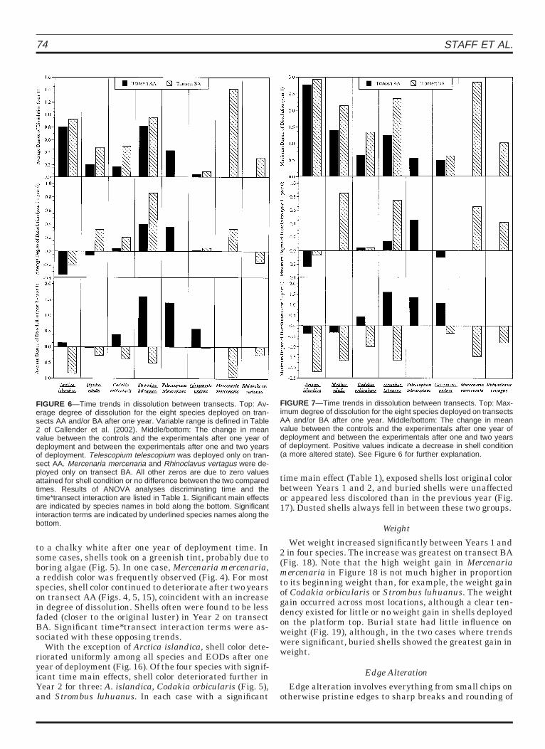
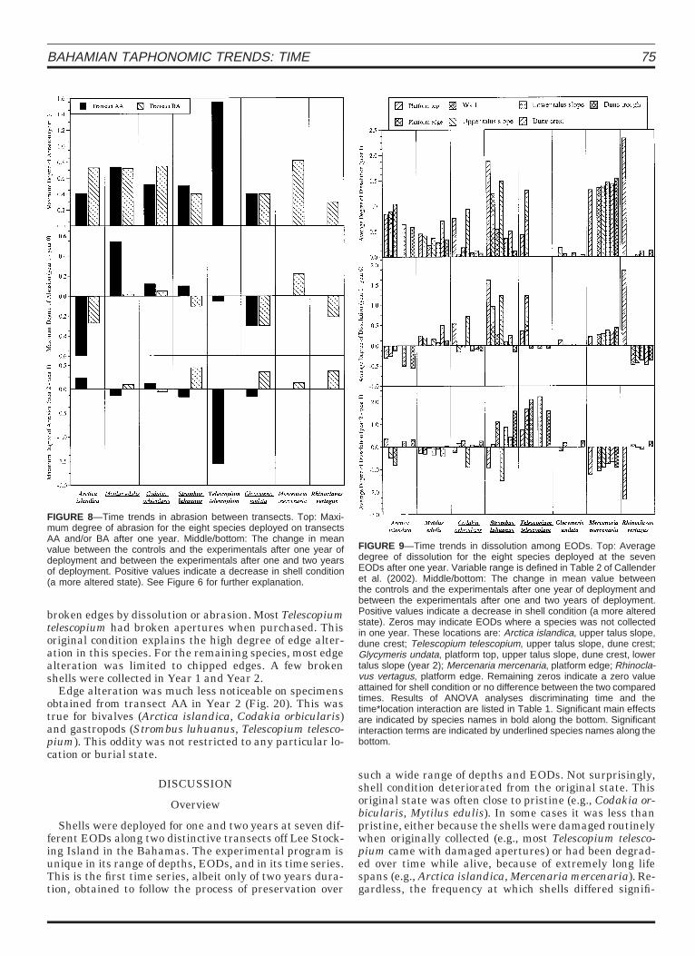
The average and maximum degree of dissolution in-creased significantly between Year 1 and Year 2 in mostspecies deployed on transect AA. The exact opposite trendwas observed on transect BA (Figs. 6 and 7) where the de-gree of dissolution appeared to decrease in Year 2. The di-ametrically opposite trends on the two transects explainthe frequency of significant time*transect interactionterms (Table 2). Abrasion changed minimally, except forTelescopium telescopium; however, significant time*transect interaction terms always were associated withopposing trends on the two transects (Fig. 8).

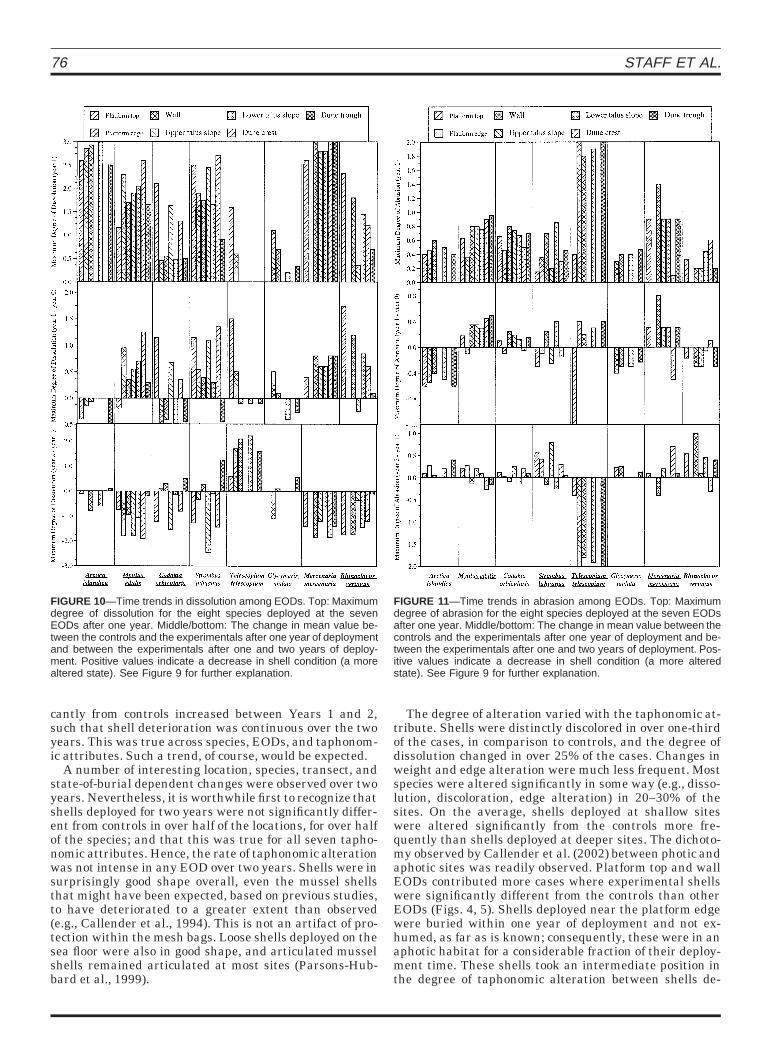
Significant differences in average degree of dissolutionover time between locations were produced by increasedevidence of dissolution in Year 2 for the gastropods, the ex-ception being Rhinoclavus vertagus, and decreased evi-dence of dissolution for the bivalves (Fig. 9). Significantdifferences in the maximum degree of dissolution wereproduced by increased dissolution in Year 2 only in Tele-scopium telescopium. For the remaining species, the de-gree of dissolution appeared to lessen in Year 2 (Fig. 10).Abrasion showed the opposite trend. Evidence of abrasionincreased in all species in Year 2, with the exception of T.telescopium (Fig. 11).

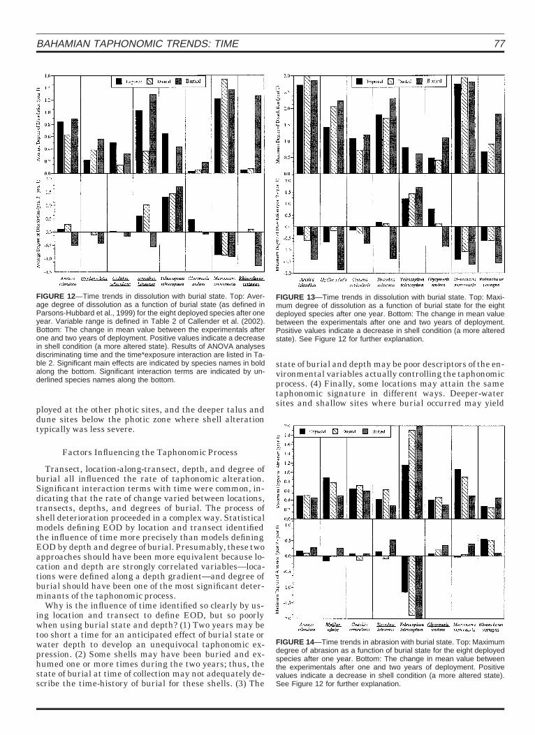
Callender et al. (2001) observed that dissolution andabrasion were inversely correlated in this data set. Thisinverse trend was not obvious in comparisons of transectsor locations, with the exception of Telescopium telesco-pium. It was very clear, however, in comparing exposurelevels. With the singular exception of T. telescopium, theaverage and maximum degree of dissolution declined inYear 2 principally or exclusively in buried shells (Figs. 12and 13). The opposite was true in abrasion (Fig. 14). Thedistinction between the time trends in buried shells andthose exposed or dusted also explains the number of sig-nificant time*exposure interaction terms.

Discoloration

Typically, shell color was faded from the original luster,if the shell was colored originally (e.g. Strombus), or faded

74 STAFF ET AL.

FIGURE 6—Time trends in dissolution between transects. Top: Av-erage degree of dissolution for the eight species deployed on tran-sects AA and/or BA after one year. Variable range is defined in Table2 of Callender et al. (2002). Middle/bottom: The change in meanvalue between the controls and the experimentals after one year ofdeployment and between the experimentals after one and two yearsof deployment. Telescopium telescopium was deployed only on tran-sect AA. Mercenaria mercenaria and Rhinoclavus vertagus were de-ployed only on transect BA. All other zeros are due to zero valuesattained for shell condition or no difference between the two comparedtimes. Results of ANOVA analyses discriminating time and thetime*transect interaction are listed in Table 1. Significant main effectsare indicated by species names in bold along the bottom. Significantinteraction terms are indicated by underlined species names along thebottom.

FIGURE 7—Time trends in dissolution between transects. Top: Max-imum degree of dissolution for the eight species deployed on transectsAA and/or BA after one year. Middle/bottom: The change in meanvalue between the controls and the experimentals after one year ofdeployment and between the experimentals after one and two yearsof deployment. Positive values indicate a decrease in shell condition(a more altered state). See Figure 6 for further explanation.

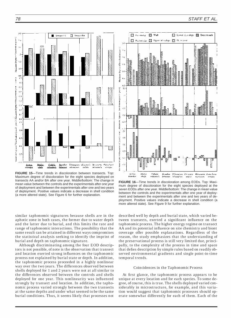
to a chalky white after one year of deployment time. Insome cases, shells took on a greenish tint, probably due toboring algae (Fig. 5). In one case, Mercenaria mercenaria,a reddish color was frequently observed (Fig. 4). For mostspecies, shell color continued to deteriorate after two yearson transect AA (Figs. 4, 5, 15), coincident with an increasein degree of dissolution. Shells often were found to be lessfaded (closer to the original luster) in Year 2 on transectBA. Significant time*transect interaction terms were as-sociated with these opposing trends.

With the exception of Arctica islandica, shell color dete-riorated uniformly among all species and EODs after oneyear of deployment (Fig. 16). Of the four species with signif-icant time main effects, shell color deteriorated further inYear 2 for three: A. islandica, Codakia orbicularis (Fig. 5),and Strombus luhuanus. In each case with a significant

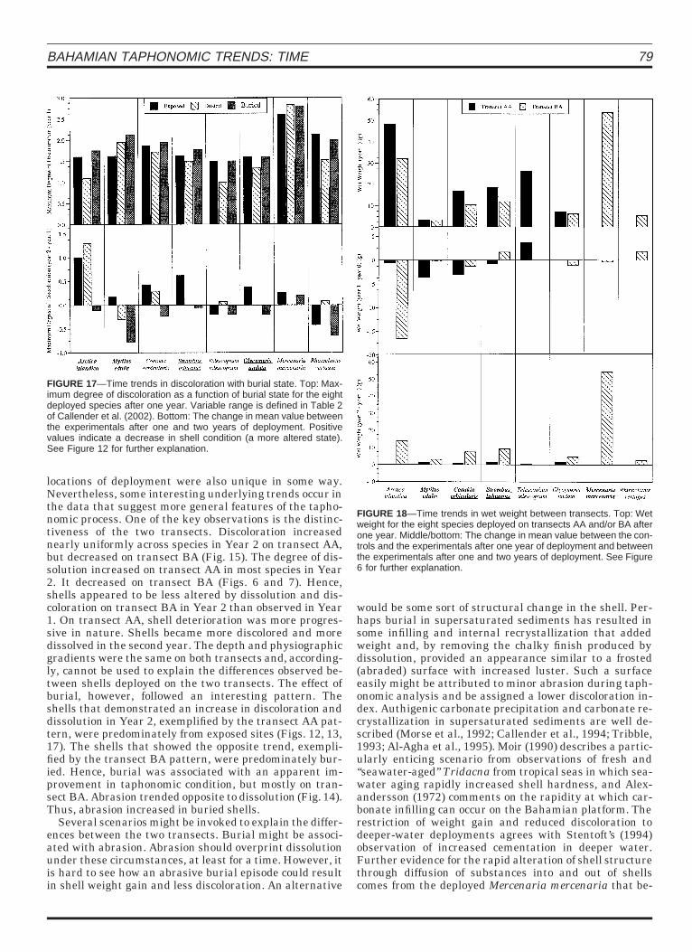
time main effect (Table 1), exposed shells lost original colorbetween Years 1 and 2, and buried shells were unaffectedor appeared less discolored than in the previous year (Fig.17). Dusted shells always fell in between these two groups.

Weight

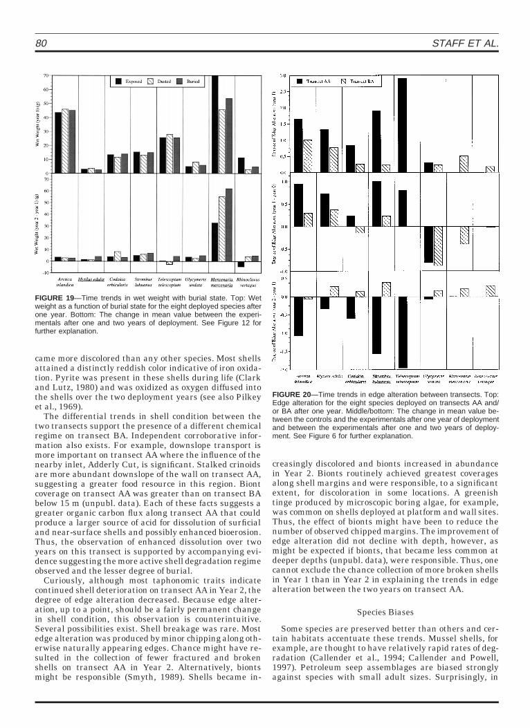
Wet weight increased significantly between Years 1 and2 in four species. The increase was greatest on transect BA(Fig. 18). Note that the high weight gain in Mercenariamercenaria in Figure 18 is not much higher in proportionto its beginning weight than, for example, the weight gainof Codakia orbicularis or Strombus luhuanus. The weightgain occurred across most locations, although a clear ten-dency existed for little or no weight gain in shells deployedon the platform top. Burial state had little influence onweight (Fig. 19), although, in the two cases where trendswere significant, buried shells showed the greatest gain inweight.

Edge Alteration

Edge alteration involves everything from small chips onotherwise pristine edges to sharp breaks and rounding of


FIGURE 8—Time trends in abrasion between transects. Top: Maxi-mum degree of abrasion for the eight species deployed on transectsAA and/or BA after one year. Middle/bottom: The change in meanvalue between the controls and the experimentals after one year ofdeployment and between the experimentals after one and two yearsof deployment. Positive values indicate a decrease in shell condition(a more altered state). See Figure 6 for further explanation.

FIGURE 9—Time trends in dissolution among EODs. Top: Averagedegree of dissolution for the eight species deployed at the sevenEODs after one year. Variable range is defined in Table 2 of Callenderet al. (2002). Middle/bottom: The change in mean value betweenthe controls and the experimentals after one year of deployment andbetween the experimentals after one and two years of deployment.Positive values indicate a decrease in shell condition (a more alteredstate). Zeros may indicate EODs where a species was not collectedin one year. These locations are: Arctica islandica, upper talus slope,dune crest; Telescopium telescopium, upper talus slope, dune crest;Glycymeris undata, platform top, upper talus slope, dune crest, lowertalus slope (year 2); Mercenaria mercenaria, platform edge; Rhinocla-vus vertagus, platform edge. Remaining zeros indicate a zero valueattained for shell condition or no difference between the two comparedtimes. Results of ANOVA analyses discriminating time and thetime*location interaction are listed in Table 1. Significant main effectsare indicated by species names in bold along the bottom. Significantinteraction terms are indicated by underlined species names along thebottom.

broken edges by dissolution or abrasion. Most Telescopiumtelescopium had broken apertures when purchased. Thisoriginal condition explains the high degree of edge alter-ation in this species. For the remaining species, most edgealteration was limited to chipped edges. A few brokenshells were collected in Year 1 and Year 2.

Edge alteration was much less noticeable on specimensobtained from transect AA in Year 2 (Fig. 20). This wastrue for bivalves (Arctica islandica, Codakia orbicularis)and gastropods (Strombus luhuanus, Telescopium telesco-pium). This oddity was not restricted to any particular lo-cation or burial state.

DISCUSSION

Overview

Shells were deployed for one and two years at seven dif-ferent EODs along two distinctive transects off Lee Stock-ing Island in the Bahamas. The experimental program isunique in its range of depths, EODs, and in its time series.This is the first time series, albeit only of two years dura-tion, obtained to follow the process of preservation over

such a wide range of depths and EODs. Not surprisingly,shell condition deteriorated from the original state. Thisoriginal state was often close to pristine (e.g., Codakia or-bicularis, Mytilus edulis). In some cases it was less thanpristine, either because the shells were damaged routinelywhen originally collected (e.g., most Telescopium telesco-pium came with damaged apertures) or had been degrad-ed over time while alive, because of extremely long lifespans (e.g., Arctica islandica, Mercenaria mercenaria). Re-gardless, the frequency at which shells differed signifi-

76 STAFF ET AL.

FIGURE 10—Time trends in dissolution among EODs. Top: Maximumdegree of dissolution for the eight species deployed at the sevenEODs after one year. Middle/bottom: The change in mean value be-tween the controls and the experimentals after one year of deploymentand between the experimentals after one and two years of deploy-ment. Positive values indicate a decrease in shell condition (a morealtered state). See Figure 9 for further explanation.

FIGURE 11—Time trends in abrasion among EODs. Top: Maximumdegree of abrasion for the eight species deployed at the seven EODsafter one year. Middle/bottom: The change in mean value between thecontrols and the experimentals after one year of deployment and be-tween the experimentals after one and two years of deployment. Pos-itive values indicate a decrease in shell condition (a more alteredstate). See Figure 9 for further explanation.

cantly from controls increased between Years 1 and 2,such that shell deterioration was continuous over the twoyears. This was true across species, EODs, and taphonom-ic attributes. Such a trend, of course, would be expected.

A number of interesting location, species, transect, andstate-of-burial dependent changes were observed over twoyears. Nevertheless, it is worthwhile first to recognize thatshells deployed for two years were not significantly differ-ent from controls in over half of the locations, for over halfof the species; and that this was true for all seven tapho-nomic attributes. Hence, the rate of taphonomic alterationwas not intense in any EOD over two years. Shells were insurprisingly good shape overall, even the mussel shellsthat might have been expected, based on previous studies,to have deteriorated to a greater extent than observed(e.g., Callender et al., 1994). This is not an artifact of pro-tection within the mesh bags. Loose shells deployed on thesea floor were also in good shape, and articulated musselshells remained articulated at most sites (Parsons-Hub-bard et al., 1999).

The degree of alteration varied with the taphonomic at-tribute. Shells were distinctly discolored in over one-thirdof the cases, in comparison to controls, and the degree ofdissolution changed in over 25% of the cases. Changes inweight and edge alteration were much less frequent. Mostspecies were altered significantly in some way (e.g., disso-lution, discoloration, edge alteration) in 20–30% of thesites. On the average, shells deployed at shallow siteswere altered significantly from the controls more fre-quently than shells deployed at deeper sites. The dichoto-my observed by Callender et al. (2002) between photic andaphotic sites was readily observed. Platform top and wallEODs contributed more cases where experimental shellswere significantly different from the controls than otherEODs (Figs. 4, 5). Shells deployed near the platform edgewere buried within one year of deployment and not ex-humed, as far as is known; consequently, these were in anaphotic habitat for a considerable fraction of their deploy-ment time. These shells took an intermediate position inthe degree of taphonomic alteration between shells de-


FIGURE 12—Time trends in dissolution with burial state. Top: Aver-age degree of dissolution as a function of burial state (as defined inParsons-Hubbard et al., 1999) for the eight deployed species after oneyear. Variable range is defined in Table 2 of Callender et al. (2002).Bottom: The change in mean value between the experimentals afterone and two years of deployment. Positive values indicate a decreasein shell condition (a more altered state). Results of ANOVA analysesdiscriminating time and the time*exposure interaction are listed in Ta-ble 2. Significant main effects are indicated by species names in boldalong the bottom. Significant interaction terms are indicated by un-derlined species names along the bottom.

FIGURE 13—Time trends in dissolution with burial state. Top: Maxi-mum degree of dissolution as a function of burial state for the eightdeployed species after one year. Bottom: The change in mean valuebetween the experimentals after one and two years of deployment.Positive values indicate a decrease in shell condition (a more alteredstate). See Figure 12 for further explanation.

FIGURE 14—Time trends in abrasion with burial state. Top: Maximumdegree of abrasion as a function of burial state for the eight deployedspecies after one year. Bottom: The change in mean value betweenthe experimentals after one and two years of deployment. Positivevalues indicate a decrease in shell condition (a more altered state).See Figure 12 for further explanation.

ployed at the other photic sites, and the deeper talus anddune sites below the photic zone where shell alterationtypically was less severe.

Factors Influencing the Taphonomic Process

Transect, location-along-transect, depth, and degree ofburial all influenced the rate of taphonomic alteration.Significant interaction terms with time were common, in-dicating that the rate of change varied between locations,transects, depths, and degrees of burial. The process ofshell deterioration proceeded in a complex way. Statisticalmodels defining EOD by location and transect identifiedthe influence of time more precisely than models definingEOD by depth and degree of burial. Presumably, these twoapproaches should have been more equivalent because lo-cation and depth are strongly correlated variables—loca-tions were defined along a depth gradient—and degree ofburial should have been one of the most significant deter-minants of the taphonomic process.

Why is the influence of time identified so clearly by us-ing location and transect to define EOD, but so poorlywhen using burial state and depth? (1) Two years may betoo short a time for an anticipated effect of burial state orwater depth to develop an unequivocal taphonomic ex-pression. (2) Some shells may have been buried and ex-humed one or more times during the two years; thus, thestate of burial at time of collection may not adequately de-scribe the time-history of burial for these shells. (3) The

state of burial and depth may be poor descriptors of the en-vironmental variables actually controlling the taphonomicprocess. (4) Finally, some locations may attain the sametaphonomic signature in different ways. Deeper-watersites and shallow sites where burial occurred may yield

78 STAFF ET AL.

FIGURE 15—Time trends in discoloration between transects. Top:Maximum degree of discoloration for the eight species deployed ontransects AA and/or BA after one year. Middle/bottom: The change inmean value between the controls and the experimentals after one yearof deployment and between the experimentals after one and two yearsof deployment. Positive values indicate a decrease in shell condition(a more altered state). See Figure 6 for further explanation.

FIGURE 16—Time trends in discoloration among EODs. Top: Maxi-mum degree of discoloration for the eight species deployed at theseven EODs after one year. Middle/bottom: The change in mean valuebetween the controls and the experimentals after one year of deploy-ment and between the experimentals after one and two years of de-ployment. Positive values indicate a decrease in shell condition (amore altered state). See Figure 9 for further explanation.

similar taphonomic signatures because shells are in theaphotic zone in both cases, the former due to water depthand the latter due to burial, and this limits the rate andrange of taphonomic interactions. The possibility that thesame result can be attained in different ways compromisesthe statistical analysis seeking to identify the imprint ofburial and depth on taphonomic signature.

Although discriminating among the four EOD descrip-tors is not possible, of note is the observation that transectand location exerted strong influences on the taphonomicprocess not explained by burial state or depth. In addition,the taphonomic process proceeded in a highly nonlinearway over the two years. The differences observed betweenshells deployed for 1 and 2 years were not at all similar tothe differences observed between the controls and shellsdeployed for one year. This nonlinearity was influencedstrongly by transect and location. In addition, the tapho-nomic process varied strongly between the two transectsat the same depths and under what seemed to be the sameburial conditions. Thus, it seems likely that processes not

described well by depth and burial state, which varied be-tween transects, exerted a significant influence on thetaphonomic process. The higher energy regime on transectAA and its potential influence on site chemistry and biontcoverage offer possible explanations. Regardless of thereason, the study emphasizes that the understanding ofthe preservational process is still very limited due, princi-pally, to the complexity of the process in time and spacethat defies description by simple rules based on readily ob-served environmental gradients and single point-in-timetemporal trends.

Coincidences in the Taphonomic Process

At first glance, the taphonomic process appears to beunique at every location and for each species. To some de-gree, of course, this is true. The shells deployed varied con-siderably in microstructure, for example, and this varia-tion would suggest that taphonomic processes should op-erate somewhat differently for each of them. Each of the


FIGURE 17—Time trends in discoloration with burial state. Top: Max-imum degree of discoloration as a function of burial state for the eightdeployed species after one year. Variable range is defined in Table 2of Callender et al. (2002). Bottom: The change in mean value betweenthe experimentals after one and two years of deployment. Positivevalues indicate a decrease in shell condition (a more altered state).See Figure 12 for further explanation.

FIGURE 18—Time trends in wet weight between transects. Top: Wetweight for the eight species deployed on transects AA and/or BA afterone year. Middle/bottom: The change in mean value between the con-trols and the experimentals after one year of deployment and betweenthe experimentals after one and two years of deployment. See Figure6 for further explanation.

locations of deployment were also unique in some way.Nevertheless, some interesting underlying trends occur inthe data that suggest more general features of the tapho-nomic process. One of the key observations is the distinc-tiveness of the two transects. Discoloration increasednearly uniformly across species in Year 2 on transect AA,but decreased on transect BA (Fig. 15). The degree of dis-solution increased on transect AA in most species in Year2. It decreased on transect BA (Figs. 6 and 7). Hence,shells appeared to be less altered by dissolution and dis-coloration on transect BA in Year 2 than observed in Year1. On transect AA, shell deterioration was more progres-sive in nature. Shells became more discolored and moredissolved in the second year. The depth and physiographicgradients were the same on both transects and, according-ly, cannot be used to explain the differences observed be-tween shells deployed on the two transects. The effect ofburial, however, followed an interesting pattern. Theshells that demonstrated an increase in discoloration anddissolution in Year 2, exemplified by the transect AA pat-tern, were predominately from exposed sites (Figs. 12, 13,17). The shells that showed the opposite trend, exempli-fied by the transect BA pattern, were predominately bur-ied. Hence, burial was associated with an apparent im-provement in taphonomic condition, but mostly on tran-sect BA. Abrasion trended opposite to dissolution (Fig. 14).Thus, abrasion increased in buried shells.

Several scenarios might be invoked to explain the differ-ences between the two transects. Burial might be associ-ated with abrasion. Abrasion should overprint dissolutionunder these circumstances, at least for a time. However, itis hard to see how an abrasive burial episode could resultin shell weight gain and less discoloration. An alternative

would be some sort of structural change in the shell. Per-haps burial in supersaturated sediments has resulted insome infilling and internal recrystallization that addedweight and, by removing the chalky finish produced bydissolution, provided an appearance similar to a frosted(abraded) surface with increased luster. Such a surfaceeasily might be attributed to minor abrasion during taph-onomic analysis and be assigned a lower discoloration in-dex. Authigenic carbonate precipitation and carbonate re-crystallization in supersaturated sediments are well de-scribed (Morse et al., 1992; Callender et al., 1994; Tribble,1993; Al-Agha et al., 1995). Moir (1990) describes a partic-ularly enticing scenario from observations of fresh and‘‘seawater-aged’’ Tridacna from tropical seas in which sea-water aging rapidly increased shell hardness, and Alex-andersson (1972) comments on the rapidity at which car-bonate infilling can occur on the Bahamian platform. Therestriction of weight gain and reduced discoloration todeeper-water deployments agrees with Stentoft’s (1994)observation of increased cementation in deeper water.Further evidence for the rapid alteration of shell structurethrough diffusion of substances into and out of shellscomes from the deployed Mercenaria mercenaria that be-

80 STAFF ET AL.

FIGURE 19—Time trends in wet weight with burial state. Top: Wetweight as a function of burial state for the eight deployed species afterone year. Bottom: The change in mean value between the experi-mentals after one and two years of deployment. See Figure 12 forfurther explanation.

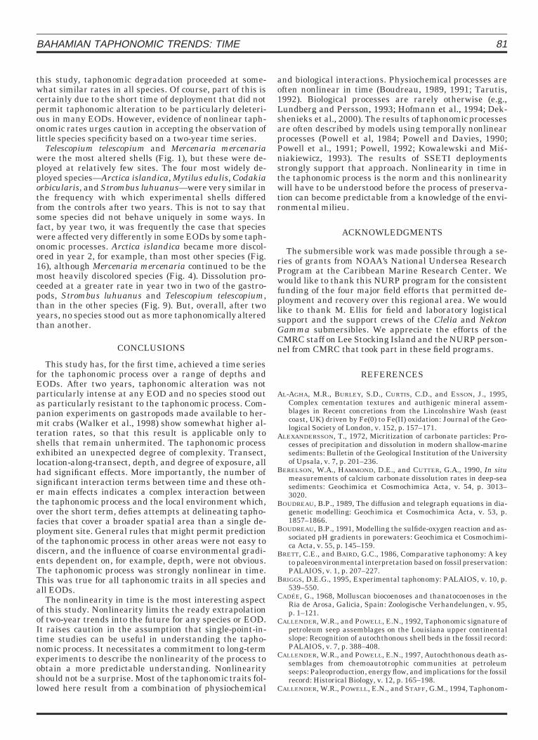
FIGURE 20—Time trends in edge alteration between transects. Top:Edge alteration for the eight species deployed on transects AA and/or BA after one year. Middle/bottom: The change in mean value be-tween the controls and the experimentals after one year of deploymentand between the experimentals after one and two years of deploy-ment. See Figure 6 for further explanation.

came more discolored than any other species. Most shellsattained a distinctly reddish color indicative of iron oxida-tion. Pyrite was present in these shells during life (Clarkand Lutz, 1980) and was oxidized as oxygen diffused intothe shells over the two deployment years (see also Pilkeyet al., 1969).

The differential trends in shell condition between thetwo transects support the presence of a different chemicalregime on transect BA. Independent corroborative infor-mation also exists. For example, downslope transport ismore important on transect AA where the influence of thenearby inlet, Adderly Cut, is significant. Stalked crinoidsare more abundant downslope of the wall on transect AA,suggesting a greater food resource in this region. Biontcoverage on transect AA was greater than on transect BAbelow 15 m (unpubl. data). Each of these facts suggests agreater organic carbon flux along transect AA that couldproduce a larger source of acid for dissolution of surficialand near-surface shells and possibly enhanced bioerosion.Thus, the observation of enhanced dissolution over twoyears on this transect is supported by accompanying evi-dence suggesting the more active shell degradation regimeobserved and the lesser degree of burial.

Curiously, although most taphonomic traits indicatecontinued shell deterioration on transect AA in Year 2, thedegree of edge alteration decreased. Because edge alter-ation, up to a point, should be a fairly permanent changein shell condition, this observation is counterintuitive.Several possibilities exist. Shell breakage was rare. Mostedge alteration was produced by minor chipping along oth-erwise naturally appearing edges. Chance might have re-sulted in the collection of fewer fractured and brokenshells on transect AA in Year 2. Alternatively, biontsmight be responsible (Smyth, 1989). Shells became in-

creasingly discolored and bionts increased in abundancein Year 2. Bionts routinely achieved greatest coveragesalong shell margins and were responsible, to a significantextent, for discoloration in some locations. A greenishtinge produced by microscopic boring algae, for example,was common on shells deployed at platform and wall sites.Thus, the effect of bionts might have been to reduce thenumber of observed chipped margins. The improvement ofedge alteration did not decline with depth, however, asmight be expected if bionts, that became less common atdeeper depths (unpubl. data), were responsible. Thus, onecannot exclude the chance collection of more broken shellsin Year 1 than in Year 2 in explaining the trends in edgealteration between the two years on transect AA.

Species Biases

Some species are preserved better than others and cer-tain habitats accentuate these trends. Mussel shells, forexample, are thought to have relatively rapid rates of deg-radation (Callender et al., 1994; Callender and Powell,1997). Petroleum seep assemblages are biased stronglyagainst species with small adult sizes. Surprisingly, in


this study, taphonomic degradation proceeded at some-what similar rates in all species. Of course, part of this iscertainly due to the short time of deployment that did notpermit taphonomic alteration to be particularly deleteri-ous in many EODs. However, evidence of nonlinear taph-onomic rates urges caution in accepting the observation oflittle species specificity based on a two-year time series.

Telescopium telescopium and Mercenaria mercenariawere the most altered shells (Fig. 1), but these were de-ployed at relatively few sites. The four most widely de-ployed species—Arctica islandica, Mytilus edulis, Codakiaorbicularis, and Strombus luhuanus—were very similar inthe frequency with which experimental shells differedfrom the controls after two years. This is not to say thatsome species did not behave uniquely in some ways. Infact, by year two, it was frequently the case that specieswere affected very differently in some EODs by some taph-onomic processes. Arctica islandica became more discol-ored in year 2, for example, than most other species (Fig.16), although Mercenaria mercenaria continued to be themost heavily discolored species (Fig. 4). Dissolution pro-ceeded at a greater rate in year two in two of the gastro-pods, Strombus luhuanus and Telescopium telescopium,than in the other species (Fig. 9). But, overall, after twoyears, no species stood out as more taphonomically alteredthan another.

CONCLUSIONS

This study has, for the first time, achieved a time seriesfor the taphonomic process over a range of depths andEODs. After two years, taphonomic alteration was notparticularly intense at any EOD and no species stood outas particularly resistant to the taphonomic process. Com-panion experiments on gastropods made available to her-mit crabs (Walker et al., 1998) show somewhat higher al-teration rates, so that this result is applicable only toshells that remain unhermited. The taphonomic processexhibited an unexpected degree of complexity. Transect,location-along-transect, depth, and degree of exposure, allhad significant effects. More importantly, the number ofsignificant interaction terms between time and these oth-er main effects indicates a complex interaction betweenthe taphonomic process and the local environment which,over the short term, defies attempts at delineating tapho-facies that cover a broader spatial area than a single de-ployment site. General rules that might permit predictionof the taphonomic process in other areas were not easy todiscern, and the influence of coarse environmental gradi-ents dependent on, for example, depth, were not obvious.The taphonomic process was strongly nonlinear in time.This was true for all taphonomic traits in all species andall EODs.

The nonlinearity in time is the most interesting aspectof this study. Nonlinearity limits the ready extrapolationof two-year trends into the future for any species or EOD.It raises caution in the assumption that single-point-in-time studies can be useful in understanding the tapho-nomic process. It necessitates a commitment to long-termexperiments to describe the nonlinearity of the process toobtain a more predictable understanding. Nonlinearityshould not be a surprise. Most of the taphonomic traits fol-lowed here result from a combination of physiochemical

and biological interactions. Physiochemical processes areoften nonlinear in time (Boudreau, 1989, 1991; Tarutis,1992). Biological processes are rarely otherwise (e.g.,Lundberg and Persson, 1993; Hofmann et al., 1994; Dek-shenieks et al., 2000). The results of taphonomic processesare often described by models using temporally nonlinearprocesses (Powell et al, 1984; Powell and Davies, 1990;Powell et al., 1991; Powell, 1992; Kowalewski and Mis-niakiewicz, 1993). The results of SSETI deploymentsstrongly support that approach. Nonlinearity in time inthe taphonomic process is the norm and this nonlinearitywill have to be understood before the process of preserva-tion can become predictable from a knowledge of the envi-ronmental milieu.

ACKNOWLEDGMENTS

The submersible work was made possible through a se-ries of grants from NOAA’s National Undersea ResearchProgram at the Caribbean Marine Research Center. Wewould like to thank this NURP program for the consistentfunding of the four major field efforts that permitted de-ployment and recovery over this regional area. We wouldlike to thank M. Ellis for field and laboratory logisticalsupport and the support crews of the Clelia and NektonGamma submersibles. We appreciate the efforts of theCMRC staff on Lee Stocking Island and the NURP person-nel from CMRC that took part in these field programs.

REFERENCES

AL-AGHA, M.R., BURLEY, S.D., CURTIS, C.D., and ESSON, J., 1995,Complex cementation textures and authigenic mineral assem-blages in Recent concretions from the Lincolnshire Wash (eastcoast, UK) driven by Fe(0) to Fe(II) oxidation: Journal of the Geo-logical Society of London, v. 152, p. 157–171.

ALEXANDERSSON, T., 1972, Micritization of carbonate particles: Pro-cesses of precipitation and dissolution in modern shallow-marinesediments: Bulletin of the Geological Institution of the Universityof Upsala, v. 7, p. 201–236.

BERELSON, W.A., HAMMOND, D.E., and CUTTER, G.A., 1990, In situmeasurements of calcium carbonate dissolution rates in deep-seasediments: Geochimica et Cosmochimica Acta, v. 54, p. 3013–3020.

BOUDREAU, B.P., 1989, The diffusion and telegraph equations in dia-genetic modelling: Geochimica et Cosmochimica Acta, v. 53, p.1857–1866.

BOUDREAU, B.P., 1991, Modelling the sulfide-oxygen reaction and as-sociated pH gradients in porewaters: Geochimica et Cosmochimi-ca Acta, v. 55, p. 145–159.

BRETT, C.E., and BAIRD, G.C., 1986, Comparative taphonomy: A keyto paleoenvironmental interpretation based on fossil preservation:PALAIOS, v. 1, p. 207–227.

BRIGGS, D.E.G., 1995, Experimental taphonomy: PALAIOS, v. 10, p.539–550.

CADEE, G., 1968, Molluscan biocoenoses and thanatocoenoses in theRia de Arosa, Galicia, Spain: Zoologische Verhandelungen, v. 95,p. 1–121.

CALLENDER, W.R., and POWELL, E.N., 1992, Taphonomic signature ofpetroleum seep assemblages on the Louisiana upper continentalslope: Recognition of autochthonous shell beds in the fossil record:PALAIOS, v. 7, p. 388–408.

CALLENDER, W.R., and POWELL, E.N., 1997, Autochthonous death as-semblages from chemoautotrophic communities at petroleumseeps: Paleoproduction, energy flow, and implications for the fossilrecord: Historical Biology, v. 12, p. 165–198.

CALLENDER, W.R., POWELL, E.N., and STAFF, G.M., 1994, Taphonom-

82 STAFF ET AL.

ic rates of molluscan shells placed in autochthonous assemblageson the Louisiana continental slope: PALAIOS, v. 9, p. 60–73.

CALLENDER, W.R., POWELL, E.N., STAFF, G.M., and DAVIES, D.J.,1992, Distinguishing autochthony, parautochthony and allo-chthony using taphofacies analysis: Can cold seep assemblages bediscriminated from assemblages of the nearshore and continentalshelf?: PALAIOS, v. 7, p. 409–421.

CALLENDER, W.R., STAFF, G.M., PARSONS-HUBBARD, K.M., POWELL,E.N., ROWE, G.T., WALKER, S.E., BRETT, C.E., RAYMOND, A.,CARL-SON, D.D., WHITE, S. and HEISE, E.A., 2002, Taphonomic trendsalong a forereef slope: Lee Stocking Island, Bahamas. I. Locationand water depth: PALAIOS, v. 17, p. 00–00.

CLARK, R.R., II, and LUTZ, R.A., 1980, Pyritization in the shells of liv-ing bivalves: Geology, v. 8, p. 268–271.

CUMMINS, H., POWELL, E.N., STANTON, R.J., JR. and STAFF, G., 1986,The rate of taphonomic loss in modern benthic habitats: Howmuch of the potentially preservable community is preserved?: Pa-laeogeography Palaeoclimatology Palaeoecology, v. 52, p.291–320.

CUTLER, A.H., 1995, Taphonomic implications of shell surface tex-tures in Bahia la Choya, northern Gulf of California: Palaeogeog-raphy Palaeoclimatology Palaeoecology, v. 114, p. 219–240.

DAVIES, D.J., STAFF, G.M., CALLENDER, W.R., and POWELL, E.N.,1990, Description of a quantitative approach to taphonomy and ta-phofacies analysis: All dead things are not created equal: in MillerIII, W., ed., Paleocommunity temporal dynamics: The long-termdevelopment of multispecies assemblages: Paleontological SocietySpecial Publications, v. 5, p. 328–350.

DEKSHENIEKS, M.M., HOFMANN, E.E., KLINCK, J.M., and POWELL,E.N., 2000, Quantifying the effects of environmental variabilityonan oyster population: A modeling study: Estuaries, v. 23, p. 593–610.

FLESSA, K.W., and BROWN, T.J., 1983, Selective solution of macroin-vertebrate calcareous hard parts: A laboratory study: Lethaia, v.16, p. 193–205.

FLESSA, K.W., CUTLER, A.H., and MELDAHL, K.H., 1993, Time and ta-phonomy: quantitative estimates of time-averaging and strati-graphic disorder in a shallow marine habitat: Paleobiology, v. 19,p. 266–286.

GLOVER, C.P., and KIDWELL, S.M., 1993, Influence of organic matrixon the post-mortem destruction of molluscan shells: Journal of Ge-ology, v. 101, p. 729–747.

HOFMANN, E.E., KLINCK, J.M., POWELL, E.N., BOYLES, S., and ELLIS,M., 1994, Modeling oyster populations II. Adult size and reproduc-tive effort: Journal of Shellfish Research, v. 13, p. 165–182.

KENDALL, C.G.STC., DILL, R.F., and SHINN, E.A., 1990, Guidebook tothe marine geology and tropical environments of Lee Stocking Is-land, the southern Exumas, Bahamas: Ken Dill Publishers, SanDiego, 82 p.

KIDWELL, S.M., in press, Organism-Sediment Interactions Sympo-sium: University of South Carolina Press.

KIDWELL, S.M., and FLESSA, K.W., 1995, The quality of the fossil re-cord: Populations, species, and communities: Annual Review ofEcology and Systematics, v. 26, p. 269–299.

KIDWELL, S.M., FURSICH, F.T., and AIGNER, T., 1986, Conceptualframework for the analysis and classification of fossil concentra-tions: PALAIOS, v. 1, p. 228–238.

KILLINGLEY, J.S., BERGER, W.H., MACDONALD, K.C., and NEWMAN,W.A., 1980, 18O/16O variations in deep-sea carbonate shells fromthe Rise hydrothermal field: Nature, v. 287, p. 218–221.

KOTTLER, E., MARTIN, R., and LIDDELL, W.D., 1992, Experimentalanalysis of abrasion and dissolution resistance of modern reefdwelling foraminifera: Implications for the preservation of biogen-ic carbonate: PALAIOS, v. 7, p. 244–276.

KOWALEWSKI, M., and MISNIAKIEWICZ, W., 1993, Reliability of quan-titative data on fossil assemblages: A model, a simulation, and anexample: Neues Jahrbuch fur Geologie und Palaontologie Abhan-dlungen, v. 187, p. 243–260.

LABARBERA, M., 1981, The ecology of Mesozoic Gryphaea, Exogyra,and Ilymatogyra (Bivalvia: Mollusca) in a modern ocean: Paleobi-ology, v. 7, p. 510–526.

LUNDBERG, S., and PERSSON, L., 1993, Optimal body size andresourcedensity: Journal of Theoretical Biology, v. 164, p. 163–180.

LUTZ, R.A., FRITZ, L.W., and CERRATO, R.N., 1988, A comparison of bi-

valve (Calyptogena magnifica) growth at two deep-sea hydrother-mal vents in the eastern Pacific: Deep-Sea Research, v. 35, p.1793–1810.

LUTZ, R.A., KENNISH, M.J., POOLEY, A.S., and FRITZ, L.W., 1994, Cal-cium carbonate dissolution rates in hydrothermal vent fields ofthe Guaymas Basin: Journal of Marine Research, v. 52, p. 969–982.

MELDAHL, K.H., and FLESSA, K.W., 1990, Taphonomic pathways andcomparative biofacies and taphofacies in a Recent intertidal shal-low shelf environment: Lethaia, v. 23, p. 43–60.

MELDAHL, K.M., FLESSA, K.W., and CUTLER, A.H., 1997, Time-aver-aging and postmortem skeletal survival in benthic fossil assem-blages: Quantitative comparison among Holocene environments:Paleobiology, v. 23, p. 207–229.

MIDDELBURG, J.J., 1989, A simple rate model for organic matter de-composition in marine sediments: Geochimica et CosmochimicaActa, v. 53, p. 1577–1581.

MOIR, B.G., 1990, Comparative studies of ‘‘fresh’’ and ‘‘aged’’ Tridacnagigas shell: Preliminary investigations of a reported technique forpretreatment of tool material: Journal of Archaeological Science,v. 17, p. 329–345.

MORSE, J.W., CORNWELL, J.C., ARAKAKI, T., LIN, S., and HUERTA-DIAZ, M., 1992, Iron sulfide and carbonate mineral diagenesis inBaffin Bay, Texas: Journal of Sedimentary Petrology, v. 62, p.671–680.

PARSONS, K.M., and BRETT, C.E., 1991, Taphonomic process and bi-ases in modern marine environments: An actualistic perspectiveon fossil assemblage preservation: in Donovan, S.K., ed., The Pro-cesses of Fossilization: Belhaven Press, London, p. 22–65.

PARSONS-HUBBARD, K.M., CALLENDER, W.R., POWELL, E.N., BRETT,C.E., WALKER, S.E., RAYMOND, A.L., and STAFF, G.M., 1999, Ratesof burial and disturbance of experimentally-deployed molluscs:Implications for preservation potential: PALAIOS, v. 14, p. 337–351.

PARSONS, K.M., POWELL, E.N., BRETT, C.E., WALKER, S.E., and CAL-LENDER, W.R., 1997, Shelf and Slope Experimental TaphonomyInitiative (SSETI): Bahamas and Gulf of Mexico: Proceedings ofthe 8th International Coral Reef Symposium, v. 2, p. 1807–1812.

PARSONS-HUBBARD, K.M., POWELL, E.N., STAFF, G.M., CALLENDER,W.R., BRETT, C.E., and WALKER, S.E., in press, The effect of burialon shell preservation and on the cover and diversity of epibionts incontinental shelf and slope environments of deposition:Organism-Sediment Interactions Symposium: University of South CarolinaPress.

PETERSON, C.H., 1983, A concept of quantitative reproductive senili-ty: Application to the hard clam, Mercenaria mercenaria (L.)?: Oec-ologia, Berlin, v. 58, p. 164–168.

PILKEY, O.H., BLACKWELDER, B.W., DOYLE, L.J., and ESTES, E.L.,1969, Environmental significance of the physical attributes of cal-careous sedimentary particles: Transactions Gulf Coast Associa-tion of Geological Societies, v. 19, p. 113–114.

POWELL, E.N., 1992, A model for death assemblage formation. Cansediment shelliness be explained?: Journal of Marine Research, v.50, p. 229–265.

POWELL, E.N., CUMMINS, H., STANTON, R.J., JR., and STAFF, G., 1984,Estimation of the size of molluscan larval settlement using thedeath assemblage: Estuarine Coastal and Shelf Science, v. 18, p.367–384.

POWELL, E.N., and DAVIES, D.J., 1990, When is an ‘‘old’’ shell reallyold?: Journal of Geology, v. 98, p. 823–844.

POWELL, E.N., KING, J.A., and BOYLES, S., 1991, Dating time-since-death of oyster shells by the rate of decomposition of the organicmatrix: Archaeometry, v. 33, p. 51–68.

POWELL, E.N., STAFF, G.M., DAVIES, D.J., and CALLENDER, W.R.,1989, Macrobenthic death assemblages in modern marine envi-ronments: Formation, interpretation and application: Critical Re-views in Aquatic Sciences, v. 1, p. 555–589.

POWELL, E.N., STANTON, R.J., JR., DAVIES, D., and LOGAN, A., 1986,Effect of a large larval settlement and catastrophic mortality onthe ecologic record of the community in the death assemblage: Es-tuarine Coastal and Shelf Science, v. 23, p. 513–525.

ROPES, J.W., MURAWSKI, S.A., and SERCHUK, F.M., 1984, Size, age,sexual maturity, and sex ratio in ocean quahogs, Arctica islandica


Linne, off Long Island, New York: United States Fish and WildlifeService, Fisheries Bulletin, v. 82, p. 253–266.

SIMON, A., POULICEK, M., VELIMIROV, B., and MACKENZIE, F.T., 1994,Comparison of anaerobic and aerobic biodegradation of mineral-ized skeletal structures in marine and estuarine conditions: Bio-geochemistry, v. 25, p. 167–195.

SMYTH, M.J., 1989, Bioerosion of gastropods shells: With emphasis oneffects of coralline algal cover and shell microstructure: CoralReefs, v. 8, p. 119–125.

SPEYER, S.E., and BRETT, C.E., 1991, Taphofacies controls back-ground and episodic processes in fossil assemblage preservation:in Allison, P.A., and Briggs, D.E.G., eds., Taphonomy: Releasingthe Data Locked in the Fossil Record: Topics in Geobiology, v. 9, p.501–545.

STAFF, G.M., and POWELL, E.N., 1990, Taphonomic signature and theimprint of taphonomic history: Discriminating between taphofa-cies of the inner continental shelf and a microtidal inlet: in MillerIII, W., ed., Paleocommunity temporal dynamics: The long-termdevelopment of multispecies assemblages: Paleontological SocietySpecial Publications, v. 5, p. 370–390.

STAFF, G., STANTON R.J., JR., POWELL, E.N., and CUMMINS, H., 1986,Time-averaging, taphonomy and their impact on paleocommunityreconstruction: Death assemblages in Texas bays: Geological So-ciety of America Bulletin, v. 97, p. 428–443.

STENTOFT, N., 1994, Early submarine cementation in fore-reef car-

bonate sediments, Barbados, West Indies: Sedimentology, v. 41, p.585–604.

TARUTIS, W.J., JR., 1992, Temperature dependence of rate constantsderived from the power model of organic matter decomposition:Geochimica Cosmochimica Acta, v. 56, p. 1387–1390.

TRIBBLE, G.W., 1993, Organic matter oxidation and aragonitediagen-esis in a coral reef: Journal of Sedimentary Petrology, v. 63, p.523–527.

TUDHOPE, A.W., and RISK, M.J., 1985, Rate of dissolution of carbonatesediments by microboring organisms, Davis Reef, Australia: Jour-nal of Sedimentary Petrology, v. 55, p. 440–447.

WALKER, S.E., 1988, Taphonomic significance of hermit crabs (Ano-mura; Paguridea): Epifaunal hermit crab-infaunal gastropod ex-ample: Palaeogeography Palaeoclimatology Palaeoecology, v. 63,p. 45–71.

WALKER, S.E., and CARLTON, J.T., 1995, Taphonomic losses becometaphonomic gains: an experimental approach using the rockyshore gastropod, Tegula funebralis: Palaeogeography Palaeocli-matology Palaeoecology, v. 114, p. 197–217.

WALKER, S.E., PARSONS-HUBBARD, K., POWELL, E.N., and BRETT,C.E., 1998, Bioerosion or bioaccumulation? Shelf-slope trends forepi- and endobionts on experimentally deployed gastropod shells:Historical Biology, v. 13, p. 61–72.

ACCEPTED JUNE 21, 2001

Documents

Taphonomic Trends Along a Forereef Slope: Lee Stocking Island, Bahamas. II. Time