ARGONNE NATIONAL LABORATORY9700 South Cass AvenueArgonne, Illinois 60439

TAO 3.9 Users Manual

Alp DenerTodd MunsonJason SarichStefan Wild

Steven BensonLois Curfman McInnes

Mathematics and Computer Science Division

Technical Memorandum ANL/MCS-TM-322

This manual is intended for use with TAO version 3.9

April 29, 2018

This product includes software produced by UChicago Argonne, LLC under Contract No.DE-AC02-06CH11357 with the Department of Energy.

Contents

Preface iii

Changes for Version 3.5 iii

Changes for Version 2.0 iii

Acknowledgments iv

License v

1 Introduction 1

2 Getting Started 32.1 Writing Application Codes with TAO . . . . . . . . . . . . . . . . . . . . . 32.2 A Simple TAO Example . . . . . . . . . . . . . . . . . . . . . . . . . . . . . 42.3 Include Files . . . . . . . . . . . . . . . . . . . . . . . . . . . . . . . . . . . 42.4 TAO Solvers . . . . . . . . . . . . . . . . . . . . . . . . . . . . . . . . . . . 42.5 Function Evaluations . . . . . . . . . . . . . . . . . . . . . . . . . . . . . . . 62.6 Programming with PETSc . . . . . . . . . . . . . . . . . . . . . . . . . . . . 6

3 Using TAO Solvers 113.1 Header File . . . . . . . . . . . . . . . . . . . . . . . . . . . . . . . . . . . . 113.2 Creation and Destruction . . . . . . . . . . . . . . . . . . . . . . . . . . . . 113.3 TAO Applications . . . . . . . . . . . . . . . . . . . . . . . . . . . . . . . . 12

3.3.1 Defining Variables . . . . . . . . . . . . . . . . . . . . . . . . . . . . 123.3.2 Application Context . . . . . . . . . . . . . . . . . . . . . . . . . . . 133.3.3 Objective Function and Gradient Routines . . . . . . . . . . . . . . 133.3.4 Hessian Evaluation . . . . . . . . . . . . . . . . . . . . . . . . . . . . 153.3.5 Bounds on Variables . . . . . . . . . . . . . . . . . . . . . . . . . . . 16

3.4 Solving . . . . . . . . . . . . . . . . . . . . . . . . . . . . . . . . . . . . . . . 163.4.1 Convergence . . . . . . . . . . . . . . . . . . . . . . . . . . . . . . . 173.4.2 Viewing Status . . . . . . . . . . . . . . . . . . . . . . . . . . . . . . 173.4.3 Obtaining a Solution . . . . . . . . . . . . . . . . . . . . . . . . . . . 183.4.4 Additional Options . . . . . . . . . . . . . . . . . . . . . . . . . . . . 18

3.5 Special Problem Structures . . . . . . . . . . . . . . . . . . . . . . . . . . . 183.5.1 PDE-Constrained Optimization . . . . . . . . . . . . . . . . . . . . . 18

i

3.5.2 Nonlinear Least Squares . . . . . . . . . . . . . . . . . . . . . . . . . 203.5.3 Complementarity . . . . . . . . . . . . . . . . . . . . . . . . . . . . . 20

4 TAO Solvers 234.1 Unconstrained Minimization . . . . . . . . . . . . . . . . . . . . . . . . . . . 23

4.1.1 Nelder-Mead Method . . . . . . . . . . . . . . . . . . . . . . . . . . 234.1.2 Limited-Memory, Variable-Metric Method . . . . . . . . . . . . . . . 244.1.3 Nonlinear Conjugate Gradient Method . . . . . . . . . . . . . . . . . 274.1.4 Newton Line Search Method . . . . . . . . . . . . . . . . . . . . . . 284.1.5 Newton Trust-Region Method . . . . . . . . . . . . . . . . . . . . . . 334.1.6 BMRM . . . . . . . . . . . . . . . . . . . . . . . . . . . . . . . . . . 354.1.7 OWL-QN . . . . . . . . . . . . . . . . . . . . . . . . . . . . . . . . . 36

4.2 Bound-Constrained Optimization . . . . . . . . . . . . . . . . . . . . . . . . 364.2.1 Projected Gradient Descent Method . . . . . . . . . . . . . . . . . . 364.2.2 Bounded Nonlinear Conjugate Gradient . . . . . . . . . . . . . . . . 364.2.3 Trust-Region Newton Method . . . . . . . . . . . . . . . . . . . . . . 364.2.4 Gradient Projection Conjugate Gradient Method . . . . . . . . . . . 374.2.5 Interior-Point Newton’s Method . . . . . . . . . . . . . . . . . . . . 374.2.6 Bound-constrained Limited-Memory Variable-Metric Method . . . . 37

4.3 PDE-Constrained Optimization . . . . . . . . . . . . . . . . . . . . . . . . . 374.3.1 Linearly-Constrained Augmented Lagrangian Method . . . . . . . . 38

4.4 Nonlinear Least-Squares . . . . . . . . . . . . . . . . . . . . . . . . . . . . . 404.4.1 POUNDerS . . . . . . . . . . . . . . . . . . . . . . . . . . . . . . . . 40

4.5 Complementarity . . . . . . . . . . . . . . . . . . . . . . . . . . . . . . . . . 434.5.1 Semismooth Methods . . . . . . . . . . . . . . . . . . . . . . . . . . 43

5 Advanced Options 455.1 Linear Solvers . . . . . . . . . . . . . . . . . . . . . . . . . . . . . . . . . . . 455.2 Monitors . . . . . . . . . . . . . . . . . . . . . . . . . . . . . . . . . . . . . . 455.3 Convergence Tests . . . . . . . . . . . . . . . . . . . . . . . . . . . . . . . . 465.4 Line Searches . . . . . . . . . . . . . . . . . . . . . . . . . . . . . . . . . . . 46

6 Adding a Solver 476.1 Header File . . . . . . . . . . . . . . . . . . . . . . . . . . . . . . . . . . . . 486.2 TAO Interface with Solvers . . . . . . . . . . . . . . . . . . . . . . . . . . . 48

6.2.1 Solver Routine . . . . . . . . . . . . . . . . . . . . . . . . . . . . . . 486.2.2 Creation Routine . . . . . . . . . . . . . . . . . . . . . . . . . . . . . 516.2.3 Destroy Routine . . . . . . . . . . . . . . . . . . . . . . . . . . . . . 526.2.4 SetUp Routine . . . . . . . . . . . . . . . . . . . . . . . . . . . . . . 526.2.5 SetFromOptions Routine . . . . . . . . . . . . . . . . . . . . . . . . 536.2.6 View Routine . . . . . . . . . . . . . . . . . . . . . . . . . . . . . . . 536.2.7 Registering the Solver . . . . . . . . . . . . . . . . . . . . . . . . . . 54

ii

Preface

The Toolkit for Advanced Optimization (TAO) focuses on the development of algorithmsand software for the solution of large-scale optimization problems on high-performancearchitectures. Areas of interest include unconstrained and bound-constrained optimization,nonlinear least squares problems, optimization problems with partial differential equationconstraints, and variational inequalities and complementarity constraints.

The development of TAO was motivated by the scattered support for parallel compu-tations and the lack of reuse of external toolkits in current optimization software. Ouraim is to produce high-quality optimization software for computing environments rangingfrom workstations and laptops to massively parallel high-performance architectures. Ourdesign decisions are strongly motivated by the challenges inherent in the use of large-scaledistributed memory architectures and the reality of working with large, often poorly struc-tured legacy codes for specific applications.

Changes in Version 3.5

TAO is now included in the PETSc distribution and the PETSc repository, thus it versionswill always match the PETSc version. The TaoSolver object is now simply Tao and thereis no TaoInitialize() or TaoFinalize(). Numerious changes have been made to make thesource code more PETSc-like. All future changes will be listed in the PETSc changesdocumentation.

Changes in Version 2.0

TAO version numbers will now adhere to the new PETSc standard of Major-Minor-Patch.Any patch-level changes will have an attempt to keep the applicatin programming interface(API) untouched, but in any case backward compatibility with previous version of the minorversion will be maintained.

Many new features and interface changes were introduced in TAO version 2.0 (andcontinue to be used in version 2.2.0). TAO applications created for previous versions willneed to be updated to work with the new version. We apologize for any inconvenience thissituation may cause; these changes were needed to keep the interface clean, clear, and easyto use. Some of the most important changes are highlighted below.

Elimination of the TaoApplication Object. The largest change to the TAO pro-gramming interface was the elimination of the TaoApplication data structure. In previousversions of TAO, this structure was created by the application programmer for application-specific data and routines. In order to more closely follow PETSc design principles, thisinformation is now directly attached to a Tao object instead. See Figure 2.1 for a listing ofwhat the most common TAO routines now look like without the TaoApplication object.

New Algorithms. TAO has a new algorithm for solving derivative-free nonlinear leastsquares problems, POUNDerS, that can efficiently solve parameter optimization problems

iii

when no derivatives are available and function evaluations are expensive. See Section 4.4.1for more information on the details of the algorithm and Section 4.4 for how to use it.TAO now also provides a new algorithm for the solution of optimization problems withpartial differential equation (PDE) constraints based on a linearly constrained augmentedLagrangian (LCL) method. More information on PDE-constrained optimization and LCLcan be found in Section 4.3.

TaoLineSearch Object. TAO has promoted the line search to a full object. Any of theavailable TAO line search algorithms (Armijo, More-Thuente, GPCG, and unit) can now beselected regardless of the overlying TAO algorithm. Users can also create new line searchalgorithms that may be more suitable for their applications. More information is availablein Section 5.4.

Better Adherence to PETSc Style. TAO now features a tighter association with PETScstandards and practices. All TAO constructs now follow PETSc conventions and are writ-ten in C. There is no longer a separate abstract class for vectors, matrices, and linearsolvers. TAO now uses these PETSc objects directly. We believe these changes make TAOapplications much easier to create and maintain for users already familiar with PETScprogramming. These changes also allow TAO to relax some of the previously imposedrequirements on the PETSc configuration. TAO now works with PETSc configured withsingle-precision and quad-precision arithmetic when using GNU compilers and no longerrequires a C++ compiler. However, TAO is not compatible with PETSc installations usingcomplex data types.

Acknowledgments

We especially thank Jorge More for his leadership, vision, and effort on previous versionsof TAO.

TAO relies on PETSc for the linear algebra required to solve optimization problems,and we have benefited from the PETSc team’s experience, tools, software, and advice. Inmany ways, TAO is a natural outcome of the PETSc development.

TAO has benefited from the work of various researchers who have provided solvers, testproblems, and interfaces. In particular, we acknowledge Lisa Grignon, Elizabeth Dolan,Boyana Norris, Gabriel Lopez-Calva, Yurii Zinchenko, Michael Gertz, Jarek Nieplocha,Limin Zhang, Manojkumar Krishnan, and Evan Gawlik. We also thank all TAO users fortheir comments, bug reports, and encouragement.

The development of TAO is supported by the Office of Advanced Scientific Comput-ing Research, Office of Science, U.S. Department of Energy, under Contract DE-AC02-06CH11357. We also thank the Argonne Laboratory Computing Resource Center and theNational Energy Research Scientific Computing Center for allowing us to test and run TAOapplications on their machines.

iv

Copyright 2013, UChicago Argonne, LLCOperator of Argonne National LaboratoryAll rights reserved.Toolkit for Advanced Optimization (TAO), Version 2.2.0OPEN SOURCE LICENSE

Redistribution and use in source and binary forms, with or without modification, are per-mitted provided that the following conditions are met:

• Redistributions of source code must retain the above copyright notice, this list of con-ditions and the following disclaimer. Software changes, modifications, or derivativeworks, should be noted with comments and the author and organization’s name.

• Redistributions in binary form must reproduce the above copyright notice, this list ofconditions and the following disclaimer in the documentation and/or other materialsprovided with the distribution.

• Neither the names of UChicago Argonne, LLC nor the Department of Energy nor thenames of its contributors may be used to endorse or promote products derived fromthis software without specific prior written permission.

• The software and the end-user documentation included with the redistribution, if any,must include the following acknowledgment:“This product includes software produced by UChicago Argonne, LLC under ContractNo. DE-AC02-06CH11357 with the Department of Energy.”

********************************************************************************DISCLAIMER

THE SOFTWARE IS SUPPLIED “AS IS” WITHOUT WARRANTY OF ANY KIND.NEITHER THE UNITED STATES GOVERNMENT, NOR THE UNITED STATESDEPARTMENT OF ENERGY, NOR UCHICAGO ARGONNE, LLC, NOR ANY OFTHEIR EMPLOYEES, MAKES ANY WARRANTY, EXPRESS OR IMPLIED, ORASSUMES ANY LEGAL LIABILITY OR RESPONSIBILITY FOR THE ACCURACY,COMPLETENESS, OR USEFULNESS OF ANY INFORMATION, DATA,APPARATUS, PRODUCT, OR PROCESS DISCLOSED, OR REPRESENTS THATITS USE WOULD NOT INFRINGE PRIVATELY OWNED RIGHTS.

********************************************************************************

v

vi

Chapter 1

Introduction

The Toolkit for Advanced Optimization (TAO) focuses on the design and implementation ofoptimization software for solving large-scale optimization applications on high-performancearchitectures. Our approach is motivated by the scattered support for parallel computationsand lack of reuse of linear algebra software in currently available optimization software. TheTAO design allows the reuse of toolkits that provide lower-level support (parallel sparsematrix data structures, preconditioners, solvers), and thus we are able to build on top ofthese toolkits instead of having to redevelop code. The advantages in terms of efficiencyand development time are significant. This chapter provides a short introduction to ourdesign philosophy and the importance of this design.

The TAO design philosophy place strong emphasis on the reuse of external tools whereappropriate. Our design enables bidirectional connection to lower-level linear algebra sup-port (e.g., parallel sparse matrix data structures) provided in toolkits such as PETSc [3, 4, 5]vas well as higher-level application frameworks. Our design decisions are strongly motivatedby the challenges inherent in the use of large-scale distributed memory architectures andthe reality of working with large and often poorly structured legacy codes for specific ap-plications. Figure 1.1 illustrates how the TAO software works with external libraries andapplication code.

The TAO solvers use fundamental PETSc objects to define and solve optimization prob-lems: vectors, matrices, index sets, and linear solvers. The concepts of vectors and matricesare standard, while an index set refers to a set of integers used to identify particular elementsof vectors or matrices. An optimization algorithm is a sequence of well-defined operationson these objects. These operations include vector sums, inner products, and matrix-vectormultiplication.

With sufficiently flexible abstract interfaces, PETSc can support a variety of imple-mentations of data structures and algorithms. These abstractions allow us to more easilyexperiment with a range of algorithmic and data structure options for realistic problems.Such capabilities are critical for making high-performance optimization software adaptableto the continual evolution of parallel and distributed architectures and the research com-munity’s discovery of new algorithms that exploit their features.

1

Linear SolversMatricesVectors Index Sets

TAO Optimization Solvers(Unconstrained, Bound, Least Squares, Complementarity)

Application Driver

Application

Initialization

Post-

ProcessingFunction and Derivative Evaluation

TAO codeUser code Interface to external

linear algebra tools

Figure 1.1: TAO Design

2

Chapter 2

Getting Started

TAO can be used on a personal computer with a single processor or within a parallelenvironment. Its basic usage involves only a few commands, but fully understanding itsusage requires time. Application programmers can easily begin to use TAO by workingwith the examples provided and then gradually learn more details according to their needs.The current version of TAO and the most recent help concerning installation and usage canbe found at http://www.mcs.anl.gov/tao.

See the PETSc users manual and http://www.mcs.anl.gov/petsc for how to installand start using PETSc/TAO.

2.1 Writing Application Codes with TAO

Examples throughout the library demonstrate the software usage and can serve as templatesfor developing custom applications. We suggest that new TAO users examine programs in

${PETSC_DIR}/src/tao/<unconstrained,bound,..>/examples/tutorials.

The HTML version of the manual pages located at

${PETSC_DIR}/docs/manpages/index.html

and

http://www.mcs.anl.gov/petsc/documentation/index.html

provides indices (organized by both routine names and concepts) to the tutorial examples.We suggest the following procedure for writing a new application program using TAO:

1. Install PETSc/TAO according to the instructions in http://www.mcs.anl.gov/petsc/

documentation/installation.html.

2. Copy an example and makefile from the directories

${PETSC_DIR}/src/tao/<unconstrained,bound,..>/examples/tutorials.

compile the example, and run the program.

3. Select the example program matching the application most closely, and use it as astarting point for developing a customized code.

3

2.2 A Simple TAO Example

To help the user start using TAO immediately, we introduce here a simple uniprocessorexample. Please read Section 3 for a more in-depth discussion on using the TAO solvers.The code presented in Figure 2.2 minimizes the extended Rosenbrock function f : Rn → Rdefined by

f(x) =m−1∑i=0

(α(x2i+1 − x22i)2 + (1− x2i)2

),

where n = 2m is the number of variables. Note that while we use the C language tointroduce the TAO software, the package is fully usable from C++ and Fortran77/90.Section ?? discusses additional issues concerning Fortran usage.

The code in Figure 2.2 contains many of the components needed to write most TAOprograms and thus is illustrative of the features present in complex optimization problems.Note that for display purposes we have omitted some nonessential lines of code as well asthe (essential) code required for the routine FormFunctionGradient, which evaluates thefunction and gradient, and the code for FormHessian, which evaluates the Hessian matrix forRosenbrock’s function. The complete code is available in $TAO_DIR/src/unconstrained/

examples/tutorials/rosenbrock1.c. The following sections annotates the lines of codein Figure 2.2.

2.3 Include Files

The include file for TAO should be used via the statement

#include <petsctao.h>

The required lower-level include files are automatically included within this high-level file.

2.4 TAO Solvers

Many TAO applications will follow an ordered set of procedures for solving an optimizationproblem: The user creates a Tao context and selects a default algorithm. Call-back routinesas well as vector (Vec) and matrix (Mat) data structures are then set. These call-backroutines will be used for evaluating the objective function, gradient, and perhaps the Hessianmatrix. The user then invokes TAO to solve the optimization problem and finally destroysthe Tao context. A list of the necessary functions for performing these steps using TAO areshown in Figure 2.1. Details of these commands are presented in Chapter 3.

4

#include "petsctao.h"

typedef struct {

PetscInt n; /* dimension */

PetscReal alpha; /* condition parameter */

} AppCtx;

/* -------------- User-defined routines ---------- */

PetscErrorCode FormFunctionGradient(Tao,Vec,PetscReal*,Vec,void*);

PetscErrorCode FormHessian(Tao,Vec,Mat,Mat,void*);

int main(int argc,char **argv)

{

PetscErrorCode ierr; /* used to check for functions returning nonzeros */

Vec x; /* solution vector */

Mat H; /* Hessian matrix */

Tao tao; /* Tao context */

AppCtx user; /* user-defined application context */

ierr = PetscInitialize(&argc,&argv,(char*)0,0);CHKERRQ(ierr);

/* Initialize problem parameters */

user.n = 2; user.alpha = 99.0;

/* Allocate vectors for the solution and gradient */

ierr = VecCreateSeq(PETSC_COMM_SELF,user.n,&x); CHKERRQ(ierr);

ierr = MatCreateSeqBAIJ(PETSC_COMM_SELF,2,user.n,user.n,1,NULL,&H);

/* Create TAO solver with desired solution method */

ierr = TaoCreate(PETSC_COMM_SELF,&tao); CHKERRQ(ierr);

ierr = TaoSetType(tao,TAOLMVM); CHKERRQ(ierr);

/* Set solution vec and an initial guess */

ierr = VecSet(x, 0); CHKERRQ(ierr);

ierr = TaoSetInitialVector(tao,x); CHKERRQ(ierr);

/* Set routines for function, gradient, hessian evaluation */

ierr = TaoSetObjectiveAndGradientRoutine(tao,FormFunctionGradient,&user);

ierr = TaoSetHessianRoutine(tao,H,H,FormHessian,&user); CHKERRQ(ierr);

/* Check for TAO command line options */

ierr = TaoSetFromOptions(tao); CHKERRQ(ierr);

/* Solve the application */

ierr = TaoSolve(tao); CHKERRQ(ierr);

/* Free data structures */

ierr = TaoDestroy(&tao); CHKERRQ(ierr);

ierr = VecDestroy(&x); CHKERRQ(ierr);

ierr = MatDestroy(&H); CHKERRQ(ierr);

ierr = PetscFinalize();

return ierr;

}

Figure 2.2: Example of Uniprocessor TAO Code

5

TaoCreate(MPI_Comm comm, Tao *tao);

TaoSetType(Tao tao, TaoType type);

TaoSetInitialVector(Tao tao, Vec x);

TaoSetObjectiveAndGradientRoutine(Tao tao,

PetscErrorCode (*FormFGradient)(Tao,Vec,PetscReal*,Vec,void*),

void *user);

TaoSetHessianRoutine(Tao tao, Mat H, Mat Hpre,

PetscErrorCode (*FormHessian)(Tao,Vec,Mat,Mat,

void*), void *user);

TaoSolve(Tao tao);

TaoDestroy(Tao tao);

Figure 2.1: Commands for Solving an Unconstrained Optimization Problem

Note that the solver algorithm selected through the function TaoSetType() can be over-ridden at runtime by using an options database. Through this database, the user not onlycan select a minimization method (e.g., limited-memory variable metric, conjugate gradient,Newton with line search or trust region) but also can prescribe the convergence tolerance,set various monitoring routines, set iterative methods and preconditions for solving thelinear systems, and so forth. See Chapter 3 for more information on the solver methodsavailable in TAO.

2.5 Function Evaluations

Users of TAO are required to provide routines that perform function evaluations. Dependingon the solver chosen, they may also have to write routines that evaluate the gradient vectorand Hessian matrix.

2.6 Programming with PETSc

TAO relies heavily on PETSc not only for its vectors, matrices, and linear solvers but alsofor its programming utilities such as command line option handling, error handling, andcompiling system. We provide here a quick overview of some of these PETSc features.Please refer to the PETSc manual [5] for a more in-depth discussion of PETSc.

Vectors

In the example in Figure 2.2, the vector data structure (Vec) is used to store the solutionand gradient for the TAO unconstrained minimization solvers. A new parallel or sequentialvector x of global dimension M is created with the command

info = VecCreate(MPI_Comm comm,int m,int M,Vec *x);

where comm denotes the MPI communicator. The type of storage for the vector may be setwith calls either to VecSetType() or to VecSetFromOptions(). Additional vectors of thesame type can be formed with

6

info = VecDuplicate(Vec old,Vec *new);

The commands

info = VecSet(Vec X,PetscScalar value);

info = VecSetValues(Vec x,int n,int *indices,

Scalar *values,INSERT_VALUES);

respectively set all the components of a vector to a particular scalar value and assigna different value to each component. More detailed information about PETSc vectors,including their basic operations, scattering/gathering, index sets, and distributed arrays,may be found in the PETSc users manual [5].

Matrices

Usage of matrices and vectors is similar. The user can create a new parallel or sequentialmatrix H with M global rows and N global columns, with the routines

ierr = MatCreate(MPI_Comm comm,Mat *H);

ierr = MatSetSizes(H,PETSC_DECIDE,PETSC_DECIDE,M,N);

where the matrix format can be specified at runtime. The user could alternatively specifyeach processes’s number of local rows and columns using m and n instead of PETSC DECIDE. Hcan then be used to store the Hessian matrix, as indicated by the call to TaoSetHessianMat().Matrix entries can be set with the command

ierr = MatSetValues(Mat H,PetscInt m,PetscInt *im, PetscInt n,

PetscInt *in, PetscScalar *values,INSERT_VALUES);

After all elements have been inserted into the matrix, it must be processed with the pair ofcommands

ierr = MatAssemblyBegin(Mat H,MAT_FINAL_ASSEMBLY);

ierr = MatAssemblyEnd(Mat H,MAT_FINAL_ASSEMBLY);

The PETSc users manual [5] discusses various matrix formats as well as the details of somebasic matrix manipulation routines.

The Options Database

A TAO application can access the command line options presented at runtime throughthe PETSc options database. This database gives the application author the ability toset and change application parameters without the need to recompile the application. Forexample, an application may have a grid discretization parameter nx that can be set withthe command line option -nx <integer>. The application can read this option with thefollowing line of code:

PetscOptionsGetInt(NULL,NULL, "-nx", &nx, &flg);

If the command line option is present, the variable nx is set accordingly; otherwise, nx

remains unchanged. A complete description of the options database may be found in thePETSc users manual [5].

7

Error Checking

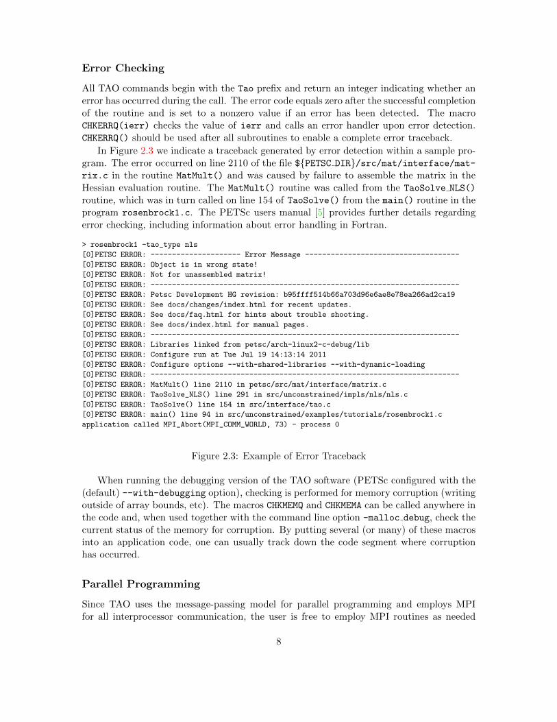
All TAO commands begin with the Tao prefix and return an integer indicating whether anerror has occurred during the call. The error code equals zero after the successful completionof the routine and is set to a nonzero value if an error has been detected. The macroCHKERRQ(ierr) checks the value of ierr and calls an error handler upon error detection.CHKERRQ() should be used after all subroutines to enable a complete error traceback.

In Figure 2.3 we indicate a traceback generated by error detection within a sample pro-gram. The error occurred on line 2110 of the file ${PETSC DIR}/src/mat/interface/mat-rix.c in the routine MatMult() and was caused by failure to assemble the matrix in theHessian evaluation routine. The MatMult() routine was called from the TaoSolve NLS()

routine, which was in turn called on line 154 of TaoSolve() from the main() routine in theprogram rosenbrock1.c. The PETSc users manual [5] provides further details regardingerror checking, including information about error handling in Fortran.

> rosenbrock1 -tao_type nls

[0]PETSC ERROR: --------------------- Error Message ------------------------------------

[0]PETSC ERROR: Object is in wrong state!

[0]PETSC ERROR: Not for unassembled matrix!

[0]PETSC ERROR: ------------------------------------------------------------------------

[0]PETSC ERROR: Petsc Development HG revision: b95ffff514b66a703d96e6ae8e78ea266ad2ca19

[0]PETSC ERROR: See docs/changes/index.html for recent updates.

[0]PETSC ERROR: See docs/faq.html for hints about trouble shooting.

[0]PETSC ERROR: See docs/index.html for manual pages.

[0]PETSC ERROR: ------------------------------------------------------------------------

[0]PETSC ERROR: Libraries linked from petsc/arch-linux2-c-debug/lib

[0]PETSC ERROR: Configure run at Tue Jul 19 14:13:14 2011

[0]PETSC ERROR: Configure options --with-shared-libraries --with-dynamic-loading

[0]PETSC ERROR: ------------------------------------------------------------------------

[0]PETSC ERROR: MatMult() line 2110 in petsc/src/mat/interface/matrix.c

[0]PETSC ERROR: TaoSolve_NLS() line 291 in src/unconstrained/impls/nls/nls.c

[0]PETSC ERROR: TaoSolve() line 154 in src/interface/tao.c

[0]PETSC ERROR: main() line 94 in src/unconstrained/examples/tutorials/rosenbrock1.c

application called MPI_Abort(MPI_COMM_WORLD, 73) - process 0

Figure 2.3: Example of Error Traceback

When running the debugging version of the TAO software (PETSc configured with the(default) --with-debugging option), checking is performed for memory corruption (writingoutside of array bounds, etc). The macros CHKMEMQ and CHKMEMA can be called anywhere inthe code and, when used together with the command line option -malloc debug, check thecurrent status of the memory for corruption. By putting several (or many) of these macrosinto an application code, one can usually track down the code segment where corruptionhas occurred.

Parallel Programming

Since TAO uses the message-passing model for parallel programming and employs MPIfor all interprocessor communication, the user is free to employ MPI routines as needed

8

throughout an application code. By default, however, the user is shielded from many of thedetails of message passing within TAO, since these are hidden within parallel objects, suchas vectors, matrices, and solvers. In addition, TAO users can interface to external tools,such as the generalized vector scatters/gathers and distributed arrays within PETSc, forassistance in managing parallel data.

The user must specify a communicator upon creation of any PETSc or TAO object(such as a vector, matrix, or solver) to indicate the processors over which the object is tobe distributed. For example, some commands for matrix, vector, and solver creation are asfollows.

ierr = MatCreate(MPI_Comm comm,Mat *H);

ierr = VecCreate(MPI_Comm comm,Vec *x);

ierr = TaoCreate(MPI_Comm comm,Tao *tao);

In most cases, the value for comm will be either PETSC COMM SELF for single-process objectsor PETSC COMM WORLD for objects distributed over all processors. The creation routines arecollective over all processors in the communicator; thus, all processors in the communicatormust call the creation routine. In addition, if a sequence of collective routines is being used,the routines must be called in the same order on each processor.

9

10

Chapter 3

Using TAO Solvers

TAO contains unconstrained minimization, bound-constrained minimization, nonlinear com-plementarity, nonlinear least squares solvers, and solvers for optimization problems withpartial differential equation constraints. The structure of these problems can differ signifi-cantly, but TAO has a similar interface to all its solvers. Routines that most solvers have incommon are discussed in this chapter. A complete list of options can be found by consultingthe manual pages. Many of the options can also be set at the command line. These optionscan also be found by running a program with the -help option.

3.1 Header File

TAO applications written in C/C++ should have the statement

#include <petsctao.h>

in each file that uses a routine in the TAO libraries.

3.2 Creation and Destruction

A TAO solver can be created by calling the

TaoCreate(MPI_Comm comm,Tao *newsolver);

routine. Much like creating PETSc vector and matrix objects, the first argument is an MPIcommunicator. An MPI [15] communicator indicates a collection of processors that will beused to evaluate the objective function, compute constraints, and provide derivative infor-mation. When only one processor is being used, the communicator PETSC COMM SELF canbe used with no understanding of MPI. Even parallel users need to be familiar with only thebasic concepts of message passing and distributed-memory computing. Most applicationsrunning TAO in parallel environments can employ the communicator PETSC COMM WORLD toindicate all processes known to PETSc in a given run.

The routine

TaoSetType(Tao tao,TaoType type);

11

can be used to set the algorithm TAO uses to solve the application. The various types ofTAO solvers and the flags that identify them will be discussed in the following chapters. Thesolution method should be carefully chosen depending on the problem being solved. Somesolvers, for instance, are meant for problems with no constraints, whereas other solvers ac-knowledge constraints in the problem and handle them accordingly. The user must also beaware of the derivative information that is available. Some solvers require second-order in-formation, while other solvers require only gradient or function information. The commandline option -tao method (or equivalently -tao type) followed by a TAO method will over-ride any method specified by the second argument. The command line option -tao method

tao lmvm, for instance, will specify the limited-memory, variable metric method for uncon-strained optimization. Note that the TaoType variable is a string that requires quotationmarks in an application program, but quotation marks are not required at the commandline.

Each TAO solver that has been created should also be destroyed by using the

TaoDestroy(Tao tao);

command. This routine frees the internal data structures used by the solver.

3.3 TAO Applications

The solvers in TAO address applications that have a set of variables, an objective function,and possibly constraints on the variables. Many solvers also require derivatives of theobjective and constraint functions. To use the TAO solvers, the application developermust define a set of variables, implement routines that evaluate the objective function andconstraint functions, and pass this information to a TAO application object.

TAO uses vector and matrix objects to pass this information from the application tothe solver. The set of variables, for instance, is represented in a vector. The gradient ofan objective function f : Rn → R, evaluated at a point, is also represented as a vector.Matrices, on the other hand, can be used to represent the Hessian of f or the Jacobian of aconstraint function c : Rn → Rm. The TAO solvers use these objects to compute a solutionto the application.

3.3.1 Defining Variables

In all the optimization solvers, the application must provide a Vec object of appropriatedimension to represent the variables. This vector will be cloned by the solvers to createadditional work space within the solver. If this vector is distributed over multiple processors,it should have a parallel distribution that allows for efficient scaling, inner products, andfunction evaluations. This vector can be passed to the application object by using the

TaoSetInitialVector(Tao,Vec);

routine. When using this routine, the application should initialize the vector with anapproximate solution of the optimization problem before calling the TAO solver. Thisvector will be used by the TAO solver to store the solution. Elsewhere in the application,this solution vector can be retrieved from the application object by using the

12

TaoGetSolutionVector(Tao,Vec *);

routine. This routine takes the address of a Vec in the second argument and sets it to thesolution vector used in the application.

3.3.2 Application Context

Writing a TAO application may require use of an application context. An applicationcontext is a structure or object defined by an application developer, passed into a routinealso written by the application developer, and used within the routine to perform its statedtask.

For example, a routine that evaluates an objective function may need parameters, workvectors, and other information. This information, which may be specific to an applicationand necessary to evaluate the objective, can be collected in a single structure and usedas one of the arguments in the routine. The address of this structure will be cast as type(void*) and passed to the routine in the final argument. Many examples of these structuresare included in the TAO distribution.

This technique offers several advantages. In particular, it allows for a uniform interfacebetween TAO and the applications. The fundamental information needed by TAO appearsin the arguments of the routine, while data specific to an application and its implementationis confined to an opaque pointer. The routines can access information created outside thelocal scope without the use of global variables. The TAO solvers and application objectswill never access this structure, so the application developer has complete freedom to defineit. If no such structure or needed by the application then a NULL pointer can be used.

3.3.3 Objective Function and Gradient Routines

TAO solvers that minimize an objective function require the application to evaluate theobjective function. Some solvers may also require the application to evaluate derivatives ofthe objective function. Routines that perform these computations must be identified to theapplication object and must follow a strict calling sequence.

Routines should follow the form

PetscErrorCode EvaluateObjective(Tao,Vec,PetscReal*,void*);

in order to evaluate an objective function f : Rn → R. The first argument is the TAOSolver object, the second argument is the n-dimensional vector that identifies where theobjective should be evaluated, and the fourth argument is an application context. Thisroutine should use the third argument to return the objective value evaluated at the pointspecified by the vector in the second argument.

This routine, and the application context, should be passed to the application object byusing the

TaoSetObjectiveRoutine(Tao,

PetscErrorCode(*)(Tao,Vec,PetscReal*,void*),

void*);

13

routine. The first argument in this routine is the TAO solver object, the second argumentis a function pointer to the routine that evaluates the objective, and the third argument isthe pointer to an appropriate application context. Although the final argument may pointto anything, it must be cast as a (void*) type. This pointer will be passed back to thedeveloper in the fourth argument of the routine that evaluates the objective. In this routine,the pointer can be cast back to the appropriate type. Examples of these structures andtheir usage are provided in the distribution.

Many TAO solvers also require gradient information from the application . The gradientof the objective function is specified in a similar manner. Routines that evaluate the gradientshould have the calling sequence

PetscErrorCode EvaluateGradient(Tao,Vec,Vec,void*);

where the first argument is the TAO solver object, the second argument is the variablevector, the third argument is the gradient vector, and the fourth argument is the user-defined application context. Only the third argument in this routine is different fromthe arguments in the routine for evaluating the objective function. The numbers in thegradient vector have no meaning when passed into this routine, but they should representthe gradient of the objective at the specified point at the end of the routine. This routine,and the user-defined pointer, can be passed to the application object by using the

TaoSetGradientRoutine(Tao,

PetscErrorCode (*)(Tao,Vec,Vec,void*),

void *);

routine. In this routine, the first argument is the Tao object, the second argument is thefunction pointer, and the third object is the application context, cast to (void*).

Instead of evaluating the objective and its gradient in separate routines, TAO also allowsthe user to evaluate the function and the gradient in the same routine. In fact, some solversare more efficient when both function and gradient information can be computed in thesame routine. These routines should follow the form

PetscErrorCode EvaluateFunctionAndGradient(Tao,Vec,

PetscReal*,Vec,void*);

where the first argument is the TAO solver and the second argument points to the inputvector for use in evaluating the function and gradient. The third argument should returnthe function value, while the fourth argument should return the gradient vector. The fifthargument is a pointer to a user-defined context. This context and the name of the routineshould be set with the call

TaoSetObjectiveAndGradientRoutine(Tao,

PetscErrorCode (*)(Tao,Vec,PetscReal*,Vec,void*),

void *);

where the arguments are the TAO application, a function name, and a pointer to a user-defined context.

The TAO example problems demonstrate the use of these application contexts as well asspecific instances of function, gradient, and Hessian evaluation routines. All these routinesshould return the integer 0 after successful completion and a nonzero integer if the functionis undefined at that point or an error occurred.

14

3.3.4 Hessian Evaluation

Some optimization routines also require a Hessian matrix from the user. The routine thatevaluates the Hessian should have the form

PetscErrorCode EvaluateHessian(Tao,Vec,Mat,Mat,void*);

where the first argument of this routine is a TAO solver object. The second argument is thepoint at which the Hessian should be evaluated. The third argument is the Hessian matrix,and the sixth argument is a user-defined context. Since the Hessian matrix is usually usedin solving a system of linear equations, a preconditioner for the matrix is often needed. Thefourth argument is the matrix that will be used for preconditioning the linear system; inmost cases, this matrix will be the same as the Hessian matrix. The fifth argument is theflag used to set the Hessian matrix and linear solver in the routine KSPSetOperators().

One can set the Hessian evaluation routine by calling the

TaoSetHessianRoutine(Tao,Mat H, Mat Hpre,

PetscErrorCode (*)(Tao,Vec,Mat,Mat,

void*), void *);

routine. The first argument is the TAO Solver object. The second and third argumentsare, respectively, the Mat object where the Hessian will be stored and the Mat object thatwill be used for the preconditioning (they may be the same). The fourth argument is thefunction that evaluates the Hessian, and the fifth argument is a pointer to a user-definedcontext, cast to (void*).

Finite Differences

Finite-difference approximations can be used to compute the gradient and the Hessianof an objective function. These approximations will slow the solve considerably and arerecommended primarily for checking the accuracy of hand-coded gradients and Hessians.These routines are

TaoDefaultComputeGradient(Tao, Vec, Vec, void*);

and

TaoDefaultComputeHessian(Tao, Vec, Mat*, Mat*,void*);

respectively. They can be set by using TaoSetGradientRoutine() and TaoSetHessianRoutine()

or through the options database with the options -tao fdgrad and -tao fd, respectively.The efficiency of the finite-difference Hessian can be improved if the coloring of the

matrix is known. If the application programmer creates a PETSc MatFDColoring object,it can be applied to the finite-difference approximation by setting the Hessian evaluationroutine to

TaoDefaultComputeHessianColor(Tao, Vec, Mat*, Mat*,void* );

and using the MatFDColoring object as the last (void *) argument to TaoSetHessianRoutine().One also can use finite-difference approximations to directly check the correctness of

the gradient and/or Hessian evaluation routines. This process can be initiated from thecommand line by using the special TAO solver tao fd test together with the option-tao test gradient or -tao test hessian.

15

Matrix-Free Methods

TAO fully supports matrix-free methods. The matrices specified in the Hessian evaluationroutine need not be conventional matrices; instead, they can point to the data required toimplement a particular matrix-free method. The matrix-free variant is allowed only whenthe linear systems are solved by an iterative method in combination with no precondition-ing (PCNONE or -pc type none), a user-provided preconditioner matrix, or a user-providedpreconditioner shell (PCSHELL). In other words, matrix-free methods cannot be used if adirect solver is to be employed. Details about using matrix-free methods are provided inthe PETSc users manual [5].

3.3.5 Bounds on Variables

Some optimization problems also impose constraints on the variables. The constraints mayimpose simple bounds on the variables or require that the variables satisfy a set of linearor nonlinear equations.

The simplest type of constraint on an optimization problem puts lower or upper boundson the variables. Vectors that represent lower and upper bounds for each variable can beset with the

TaoSetVariableBounds(Tao,Vec,Vec);

command. The first vector and second vector should contain the lower and upper bounds,respectively. When no upper or lower bound exists for a variable, the bound may be set toTAO INFINITY or TAO NINFINITY. After the two bound vectors have been set, they may beaccessed with the command TaoGetVariableBounds().

Alternatively, it may be more convenient for the user to designate a routine for com-puting these bounds that the solver will call before starting its algorithm. This routine willhave the form

PetscErrorCode EvaluateBounds(Tao,Vec,Vec,void*);

where the two vectors, representing the lower and upper bounds respectfully, will be com-puted.

This routine can be set with the

TaoSetVariableBoundsRoutine(Tao

PetscErrorCode (*)(Tao,Vec,Vec,void*),void*);

command.Since not all solvers recognize the presence of bound constraints on variables, the user

must be careful to select a solver that acknowledges these bounds.

3.4 Solving

Once the application and solver have been set up, the solver can be called by using the

TaoSolve(Tao);

routine. We discuss several universal options below.

16

3.4.1 Convergence

Although TAO and its solvers set default parameters that are useful for many problems, theuser may need to modify these parameters in order to change the behavior and convergenceof various algorithms.

One convergence criterion for most algorithms concerns the number of digits of accuracyneeded in the solution. In particular, the convergence test employed by TAO attempts tostop when the error in the constraints is less than εcrtol and either

||g(X)|| ≤ εgatol,||g(X)||/|f(X)| ≤ εgrtol, or||g(X)||/|g(X0)| ≤ εgttol,

where X is the current approximation to the true solution X∗ and X0 is the initial guess.X∗ is unknown, so TAO estimates f(X) − f(X∗) with either the square of the norm ofthe gradient or the duality gap. A relative tolerance of εfrtol = 0.01 indicates that twosignificant digits are desired in the objective function. Each solver sets its own convergencetolerances, but they can be changed by using the routine TaoSetTolerances(). Anotherset of convergence tolerances terminates the solver when the norm of the gradient function(or Lagrangian function for bound-constrained problems) is sufficiently close to zero.

Other stopping criteria include a minimum trust-region radius or a maximum number ofiterations. These parameters can be set with the routines TaoSetTrustRegionTolerance()and TaoSetMaximumIterations(). Similarly, a maximum number of function evaluationscan be set with the command TaoSetMaximumFunctionEvaluations(). -tao max it, and-tao max funcs.

3.4.2 Viewing Status

To see parameters and performance statistics for the solver, the routine

TaoView(Tao tao)

can be used. This routine will display to standard output the number of function evaluationsneed by the solver and other information specific to the solver. This same output can beproduced by using the command line option -tao view.

The progress of the optimization solver can be monitored with the runtime option-tao monitor. Although monitoring routines can be customized, the default monitoringroutine will print out several relevant statistics to the screen.

The user also has access to information about the current solution. The current iterationnumber, objective function value, gradient norm, infeasibility norm, and step length can beretrieved with the follwing command.

TaoGetSolutionStatus(Tao tao, PetscInt *iterate, PetscReal *f,

PetscReal *gnorm, PetscReal *cnorm, PetscReal *xdiff,

TaoConvergedReason *reason)

The last argument returns a code that indicates the reason that the solver terminated.Positive numbers indicate that a solution has been found, while negative numbers indicatea failure. A list of reasons can be found in the manual page for TaoGetConvergedReason().

17

3.4.3 Obtaining a Solution

After exiting the TaoSolve() function, the solution, gradient, and dual variables (if avail-able) can be recovered with the following routines.

TaoGetSolutionVector(Tao, Vec *X);

TaoGetGradientVector(Tao, Vec *G);

TaoComputeDualVariables(Tao, Vec X, Vec Duals);

Note that the Vec returned by TaoGetSolutionVector will be the same vector passedto TaoSetInitialVector. This information can be obtained during user-defined routinessuch as a function evaluation and customized monitoring routine or after the solver hasterminated.

3.4.4 Additional Options

Additional options for the TAO solver can be be set from the command line by using the

TaoSetFromOptions(Tao)

routine. This command also provides information about runtime options when the userincludes the -help option on the command line.

3.5 Special Problem Structures

Below we discuss how to exploit the special structures for three classes of problems thatTAO solves.

3.5.1 PDE-Constrained Optimization

TAO can solve PDE-constrained optimization applications of the form

minu,v

f(u, v)

subject to g(u, v) = 0,

where the state variable u is the solution to the discretized partial differential equationdefined by g and parametrized by the design variable v, and f is an objective function.In this case, the user needs to set routines for computing the objective function and itsgradient, the constraints, and the Jacobian of the constraints with respect to the state anddesign variables. TAO also needs to know which variables in the solution vector correspondto state variables and which to design variables.

The objective and gradient routines are set as for other TAO applications, with TaoSet-

ObjectiveRoutine() and TaoSetGradientRoutine(). The user can also provide a fusedobjective function and gradient evaluation with TaoSetObjectiveAndGradientRoutine().The input and output vectors include the combined state and design variables. Index setsfor the state and design variables must be passed to TAO by using the function

TaoSetStateDesignIS(Tao, IS, IS);

18

where the first IS is a PETSc IndexSet containing the indices of the state variables and thesecond IS the design variables.

Nonlinear equation constraints have the general form c(x) = 0, where c : Rn → Rm.These constraints should be specified in a routine, written by the user, that evaluates c(x).The routine that evaluates the constraint equations should have the form

PetscErrorCode EvaluateConstraints(Tao,Vec,Vec,void*);

The first argument of this routine is a TAO solver object. The second argument is thevariable vector at which the constraint function should be evaluated. The third argumentis the vector of function values c(x), and the fourth argument is a pointer to a user-definedcontext. This routine and the user-defined context should be set in the TAO solver withthe

TaoSetConstraintsRoutine(Tao,Vec,

PetscErrorCode (*)(Tao,Vec,Vec,void*),

void*);

command. In this function, the first argument is the TAO solver object, the second ar-gument a vector in which to store the constraints, the third argument is a function pointto the routine for evaluating the constraints, and the fourth argument is a pointer to auser-defined context.

The Jacobian of c(x) is the matrix in Rm×n such that each column contains the partialderivatives of c(x) with respect to one variable. The evaluation of the Jacobian of c shouldbe performed by calling the

PetscErrorCode JacobianState(Tao,Vec,Mat,Mat,Mat,void*);

PetscErrorCode JacobianDesign(Tao,Vec,Mat*,void*);

routines. In these functions, The first arguemnt is the TAO solver object. The secondargument is the variable vector at which to evaluate the Jacobian matrix, the third argumentis the Jacobian matrix, and the last argument is a pointer to a user-defined context. Thefourth and fifth arguments of the Jacobian evaluation with respect to the state variablesare for providing PETSc matrix objects for the preconditioner and for applying the inverseof the state Jacobian, respectively. This inverse matrix may be PETSC NULL, in which caseTAO will use a PETSc Krylov subspace solver to solve the state system. These evaluationroutines should be registered with TAO by using the

TaoSetJacobianStateRoutine(Tao,Mat,Mat,Mat,

PetscErrorCode (*)(Tao,Vec,Mat,Mat,

void*), void*);

TaoSetJacobianDesignRoutine(Tao,Mat,

PetscErrorCode (*)(Tao,Vec,Mat*,void*),

void*);

routines. The first argument is the TAO solver object, and the second argument is thematrix in which the Jacobian information can be stored. For the state Jacobian, the thirdargument is the matrix that will be used for preconditioning, and the fourth argument is

19

an optional matrix for the inverse of the state Jacobian. One can use PETSC NULL for thisinverse argument and let PETSc apply the inverse using a KSP method, but faster resultsmay be obtained by manipulating the structure of the Jacobian and providing an inverse.The fifth argument is the function pointer, and the sixth argument is an optional user-defined context. Since no solve is performed with the design Jacobian, there is no need toprovide preconditioner or inverse matrices.

3.5.2 Nonlinear Least Squares

For nonlinear least squares applications, we are solving the optimization problem

minx

∑i

(fi(x)− di)2.

For these problems, the objective function value should be computed as a vector of residuals,fi(x)−di, for better algorithmic results using a separable objective function, computed witha function of the form

PetscErrorCode EvaluateSeparableFunction(Tao,Vec,Vec,void*);

and set with the

TaoSetSeparableObjectiveRoutine(Tao,

PetscErrorCode (*)(Tao,Vec,Vec,void*),

void *);

routine.

3.5.3 Complementarity

Complementarity applications have equality constraints in the form of nonlinear equationsC(X) = 0, where C : Rn → Rm. These constraints should be specified in a routine writtenby the user with the form

PetscErrorCode EqualityConstraints(Tao,Vec,Vec,void*);

that evaluates C(X). The first argument of this routine is a TAO Solver object. The secondargument is the variable vector X at which the constraint function should be evaluated.The third argument is the output vector of function values C(X), and the fourth argumentis a pointer to a user-defined context.

This routine and the user-defined context must be registered with TAO by using the

TaoSetConstraintRoutine(Tao, Vec,

PetscErrorCode (*)(Tao,Vec,Vec,void*),

void*);

command. In this command, the first argument is TAO Solver object, the second argumentis vector in which to store the function values, the third argument is the user-defined routinethat evaluates C(X), and the fourth argument is a pointer to a user-defined context thatwill be passed back to the user.

20

The Jacobian of the function is the matrix in Rm×n such that each column contains thepartial derivatives of f with respect to one variable. The evaluation of the Jacobian of Cshould be performed in a routine of the form

PetscErrorCode EvaluateJacobian(Tao,Vec,Mat,Mat,void*);

In this function, the first argument is the TAO Solver object and the second argumentis the variable vector at which to evaluate the Jacobian matrix. The third argument isthe Jacobian matrix, and the sixth argument is a pointer to a user-defined context. Sincethe Jacobian matrix may be used in solving a system of linear equations, a preconditionerfor the matrix may be needed. The fourth argument is the matrix that will be used forpreconditioning the linear system; in most cases, this matrix will be the same as the Hessianmatrix. The fifth argument is the flag used to set the Jacobian matrix and linear solver inthe routine KSPSetOperators().

This routine should be specified to TAO by using the

TaoSetJacobianRoutine(Tao,Mat J, Mat Jpre,

PetscErrorCode (*)(Tao,Vec,Mat,Mat,

void*), void*);

command. The first argument is the TAO Solver object; the second and third argumentsare the Mat objects in which the Jacobian will be stored and the Mat object that will beused for the preconditioning (they may be the same), respectively. The fourth argumentis the function pointer; and the fifth argument is an optional user-defined context. TheJacobian matrix should be created in a way such that the product of it and the variablevector can be stored in the constraint vector.

21

22

Chapter 4

TAO Solvers

TAO includes a variety of optimization algorithms for several classes of problems (uncon-strained, bound-constrained, and PDE-constrained minimization, nonlinear least-squares,and complementarity). The TAO algorithms for solving these problems are detailed in thissection, a particular algorithm can chosen by using the TaoSetType() function or usingthe command line arguments -tao type <name>. For those interested in extending thesealgorithms or using new ones, please see Chapter 6 for more information.

4.1 Unconstrained Minimization

Unconstrained minimization is used to minimize a function of many variables without anyconstraints on the variables, such as bounds. The methods available in TAO for solvingthese problems can be classified according to the amount of derivative information required:

1. Function evaluation only – Nelder-Mead method (tao nm)

2. Function and gradient evaluations – limited-memory, variable-metric method (tao lmvm)and nonlinear conjugate gradient method (tao cg)

3. Function, gradient, and Hessian evaluations – Newton line search method (tao nls)and Newton trust-region method (tao ntr)

The best method to use depends on the particular problem being solved and the accuracyrequired in the solution. If a Hessian evaluation routine is available, then the Newtonline search and Newton trust-region methods will likely perform best. When a Hessianevaluation routine is not available, then the limited-memory, variable-metric method islikely to perform best. The Nelder-Mead method should be used only as a last resort whenno gradient information is available.

Each solver has a set of options associated with it that can be set with command linearguments. These algorithms and the associated options are briefly discussed in this chapter.

4.1.1 Nelder-Mead Method

The Nelder-Mead algorithm [26] is a direct search method for finding a local minimum ofa function f(x). This algorithm does not require any gradient or Hessian information of

23

f and therefore has some expected advantages and disadvantages compared to the otherTAO solvers. The obvious advantage is that it is easier to write an application when noderivatives need to be calculated. The downside is that this algorithm can be slow toconverge or can even stagnate, and it performs poorly for large numbers of variables.

This solver keeps a set of N + 1 sorted vectors x1, x2, . . . , xN+1 and their correspondingobjective function values f1 ≤ f2 ≤ . . . ≤ fN+1. At each iteration, xN+1 is removed fromthe set and replaced with

x(µ) = (1 + µ)1

N

N∑i=1

xi − µxN+1,

where µ can be one of µ0, 2µ0,12µ0,−

12µ0 depending on the values of each possible f(x(µ)).

The algorithm terminates when the residual fN+1 − f1 becomes sufficiently small. Be-cause of the way new vectors can be added to the sorted set, the minimum function valueand/or the residual may not be impacted at each iteration.

Two options can be set specifically for the Nelder-Mead algorithm:

-tao nm lamda <value> sets the initial set of vectors (x0 plus value in each coordinatedirection); the default value is 1.

-tao nm mu <value> sets the value of µ0; the default is µ0 = 1.

4.1.2 Limited-Memory, Variable-Metric Method

The limited-memory, variable-metric method computes a positive definite approximation tothe Hessian matrix from a limited number of previous iterates and gradient evaluations. Adirection is then obtained by solving the system of equations

Hkdk = −∇f(xk),

where Hk is the Hessian approximation obtained by using the BFGS update formula. Theinverse of Hk can readily be applied to obtain the direction dk. Having obtained the direc-tion, a More-Thuente line search is applied to compute a step length, τk, that approximatelysolves the one-dimensional optimization problem

minτf(xk + τdk).

The current iterate and Hessian approximation are updated, and the process is repeateduntil the method converges. This algorithm is the default unconstrained minimization solverand can be selected by using the TAO solver tao lmvm. For best efficiency, function andgradient evaluations should be performed simultaneously when using this algorithm.

The primary factors determining the behavior of this algorithm are the number of vec-tors stored for the Hessian approximation and the scaling matrix used when computingthe direction. The number of vectors stored can be set with the command line argument-tao lmm vectors <int>; 5 is the default value. Increasing the number of vectors resultsin a better Hessian approximation and can decrease the number of iterations required to

24

compute a solution to the optimization problem. However, as the number of vectors in-creases, more memory is consumed, and each direction calculation takes longer to compute.Therefore, a tradeoff must be made between the quality of the Hessian approximation, thememory requirements, and the time to compute the direction. A list of all available optionsfor this algorithm is presented in Table 4.1.

During the computation of the direction, the inverse of an “initial” positive-definite Hes-sian approximation H0,k is applied. This approximation can be updated at each iteration.The choice of H0,k significantly affects the quality of the direction obtained and can resultin a decrease in the number of function and gradient evaluations required to solve the opti-mization problem. However, the calculation of H0,k at each iteration significantly affects thetime required to update the limited-memory BFGS approximation and the cost of obtainingthe direction. By default, H0,k is a diagonal matrix obtained from the diagonal entries ofa Broyden approximation to the Hessian matrix. The calculation of H0,k can be modifiedwith the command line argument -tao lmm scale type <none,scalar,broyden>. Eachscaling method is described below. The scalar and broyden techniques are inspired by[13].

none This scaling method uses the identity matrix as H0,k. No extra computations arerequired when obtaining the search direction or updating the Hessian approximation.However, the number of functions and gradient evaluations required to converge to asolution is typically much larger than the number required when using other scalingmethods.

scalar This scaling method uses a multiple of the identity matrix as H0,k. The scalar valueσ is chosen by solving the one-dimensional optimization problem

minσ‖σαY − σα−1S‖2F ,

where α ∈ [0, 1] is given and S and Y are the matrices of past iterate and gradientinformation required by the limited-memory BFGS update formula. The optimal valuefor σ can be written down explicitly. This choice of σ attempts to satisfy the secantequation σY = S. Since this equation cannot typically be satisfied by a scalar, a leastnorm solution is computed. The amount of past iterate and gradient information usedis set by the command line argument -tao lmm scalar history <int>, which mustbe less than or equal to the number of vectors kept for the BFGS approximation.The default value is 5. The choice for α is made with the command line argument-tao lmm scalar alpha <real>; 1 is the default value. This scaling method offers agood compromise between no scaling and broyden scaling.

broyden This scaling method uses a positive-definite diagonal matrix obtained from thediagonal entries of the Broyden approximation to the Hessian for the scaling matrix.The Broyden approximation is a family of approximations parametrized by a constantφ; φ = 0 gives the BFGS formula, and φ = 1 gives the DFP formula. The value of φis set with the command line argument -tao lmm broyden phi <real>; the defaultvalue is 0.125. This scaling method requires the most computational effort of theavailable choices but typically results in a significant reduction in the number offunction and gradient evaluations taken to compute a solution.

25

An additional rescaling of the diagonal matrix can be applied to further improve per-formance when using the broyden scaling method. The rescaling method can be set withthe command line argument -tao lmm rescale type <none,scalar,gl>; scalar is thedefault rescaling method. The rescaling method applied can have a large impact on thenumber of function and gradient evaluations necessary to compute a solution to the opti-mization problem, but it increases the time required to update the BFGS approximation.Each rescaling method is described below. These techniques are inspired by [13].

none This rescaling method does not modify the diagonal scaling matrix.

scalar This rescaling method chooses a scalar value σ by solving the one-dimensionaloptimization problem

minσ‖σαHβ

0,kY − σα−1Hβ−1

0,k S‖2F ,

where α ∈ [0, 1] and β ∈ [0, 1] are given, H0,k is the positive-definite diagonal scal-ing matrix computed by using the Broyden update, and S and Y are the matricesof past iterate and gradient information required by the limited-memory BFGS up-date formula, respectfully. This choice of σ attempts to satisfy the secant equationσH0,kY = S. Since this equation cannot typically be satisfied by a scalar, a leastnorm solution is computed. The scaling matrix used is then σH0,k. The amountof past iterate and gradient information used is set by the command line argument-tao lmm rescale history <int>, which must be less than or equal to the num-ber of vectors kept for the BFGS approximation; the default value is 5. The choicefor α is made with the command line argument -tao lmm rescale alpha <real>;1 is the default value. The choice for β is made with the command line argument-tao lmm rescale beta <real>; 0.5 is the default value.

gl This scaling method is the same as the scalar rescaling method, but the previous valuefor the scaling matrix H0,k−1 is used when computing σ. This is the rescaling methodsuggested in [13].

A limit can be placed on the difference between the scaling matrix computed at thisiteration and the previous value for the scaling matrix. The limiting type can be set withthe command line argument -tao lmm limit type <none,average,relative,absolute>;none is the default value. Each of these methods is described below when using the scalar

scaling method. The techniques are the same when using the broyden scaling method butare applied to each entry in the diagonal matrix.

none Set σk = σ, where σ is the value computed by the scaling method.

average Set σk = µσ+ (1−µ)σk−1, where σ is the value computed by the scaling method,σk−1 is the previous value, and µ ∈ [0, 1] is given.

relative Set σk = median {(1− µ)σk−1, σ, (1 + µ)σk−1}, where σ is the value computedby the scaling method, σk−1 is the previous value, and µ ∈ [0, 1] is given.

absolute Set σk = median {σk−1 − ν, σ, σk−1 + ν}, where σ is the value computed by thescaling method, σk−1 is the previous value, and ν is given.

26

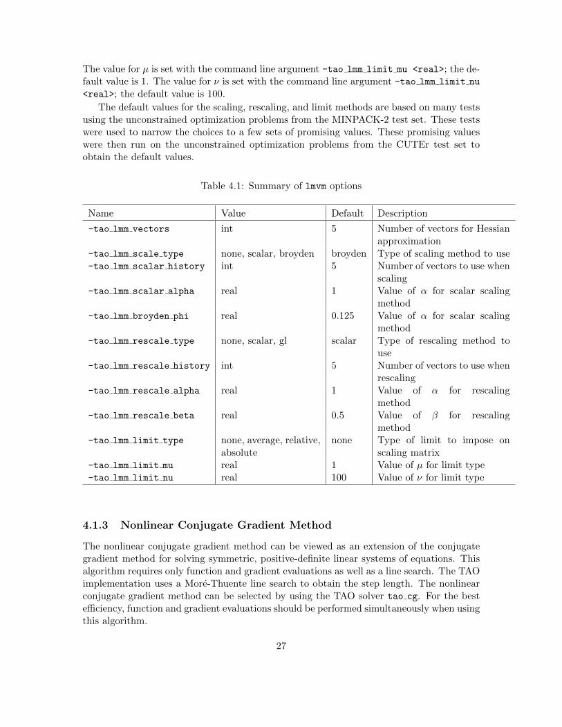
The value for µ is set with the command line argument -tao lmm limit mu <real>; the de-fault value is 1. The value for ν is set with the command line argument -tao lmm limit nu

<real>; the default value is 100.

The default values for the scaling, rescaling, and limit methods are based on many testsusing the unconstrained optimization problems from the MINPACK-2 test set. These testswere used to narrow the choices to a few sets of promising values. These promising valueswere then run on the unconstrained optimization problems from the CUTEr test set toobtain the default values.

Table 4.1: Summary of lmvm options

Name Value Default Description

-tao lmm vectors int 5 Number of vectors for Hessianapproximation

-tao lmm scale type none, scalar, broyden broyden Type of scaling method to use-tao lmm scalar history int 5 Number of vectors to use when

scaling-tao lmm scalar alpha real 1 Value of α for scalar scaling

method-tao lmm broyden phi real 0.125 Value of α for scalar scaling

method-tao lmm rescale type none, scalar, gl scalar Type of rescaling method to

use-tao lmm rescale history int 5 Number of vectors to use when

rescaling-tao lmm rescale alpha real 1 Value of α for rescaling

method-tao lmm rescale beta real 0.5 Value of β for rescaling

method-tao lmm limit type none, average, relative,

absolutenone Type of limit to impose on

scaling matrix-tao lmm limit mu real 1 Value of µ for limit type-tao lmm limit nu real 100 Value of ν for limit type

4.1.3 Nonlinear Conjugate Gradient Method

The nonlinear conjugate gradient method can be viewed as an extension of the conjugategradient method for solving symmetric, positive-definite linear systems of equations. Thisalgorithm requires only function and gradient evaluations as well as a line search. The TAOimplementation uses a More-Thuente line search to obtain the step length. The nonlinearconjugate gradient method can be selected by using the TAO solver tao cg. For the bestefficiency, function and gradient evaluations should be performed simultaneously when usingthis algorithm.

27

Five variations are currently supported by the TAO implementation: the Fletcher-Reeves method, the Polak-Ribiere method, the Polak-Ribiere-Plus method [27], the Hestenes-Stiefel method, and the Dai-Yuan method. These conjugate gradient methods can be speci-fied by using the command line argument -tao cg type <fr,pr,prp,hs,dy>, respectively.The default value is prp.

The conjugate gradient method incorporates automatic restarts when successive gradi-ents are not sufficiently orthogonal. TAO measures the orthogonality by dividing the innerproduct of the gradient at the current point and the gradient at the previous point by thesquare of the Euclidean norm of the gradient at the current point. When the absolute valueof this ratio is greater than η, the algorithm restarts using the gradient direction. Theparameter η can be set by using the command line argument -tao cg eta <real>; 0.1 isthe default value.

4.1.4 Newton Line Search Method

The Newton line search method solves the symmetric system of equations

Hkdk = −gk

to obtain a step dk, where Hk is the Hessian of the objective function at xk and gk isthe gradient of the objective function at xk. For problems where the Hessian matrix isindefinite, the perturbed system of equations

(Hk + ρkI)dk = −gk

is solved to obtain the direction, where ρk is a positive constant. If the direction computedis not a descent direction, the (scaled) steepest descent direction is used instead. Havingobtained the direction, a More-Thuente line search is applied to obtain a step length, τk,that approximately solves the one-dimensional optimization problem

minτf(xk + τdk).

The Newton line search method can be selected by using the TAO solver tao nls. Theoptions available for this solver are listed in Table 4.2. For the best efficiency, function andgradient evaluations should be performed simultaneously when using this algorithm.

The system of equations is approximately solved by applying the conjugate gradientmethod, Nash conjugate gradient method, Steihaug-Toint conjugate gradient method, gen-eralized Lanczos method, or an alternative Krylov subspace method supplied by PETSc.The method used to solve the systems of equations is specified with the command line ar-gument -tao nls ksp type <cg,nash,stcg,gltr,petsc>; stcg is the default. When thetype is set to petsc, the method set with the PETSc -ksp type command line argumentis used. For example, to use GMRES as the linear system solver, one would use the com-mand line arguments -tao nls ksp type petsc -ksp type gmres. Internally, the PETScimplementations for the conjugate gradient methods and the generalized Lanczos methodare used. See the PETSc manual for further information on changing the behavior of thelinear system solvers.

28

Table 4.2: Summary of nls options

Name Value Default Description

-tao nls ksp type cg, nash, stcg, gltr,petsc

stcg Type of Krylov subspacemethod to use when solvinglinear system

-tao nls pc type none, ahess, bfgs,petsc

bfgs Type of preconditioner to usewhen solving linear system

-tao nls bfgs scale type ahess, phess, bfgs phess Type of scaling matrix to usewith BFGS preconditioner

-tao nls sval real 0 Initial perturbation value-tao nls imin real 10−4 Minimum initial perturbation

value-tao nls imax real 100 Maximum initial perturbation

value-tao nls imfac real 0.1 Factor applied to norm of gra-

dient when initializing pertur-bation

-tao nls pmax real 100 Maximum perturbation whenincreasing value

-tao nls pgfac real 10 Growth factor applied toperturbation when increasingvalue

-tao nls pmgfac real 0.1 Factor applied to norm of gra-dient when increasing pertur-bation

-tao nls pmin real 10−12 Minimum perturbation whendecreasing value; smaller val-ues set to zero

-tao nls psfac real 0.4 Shrink factor applied to per-turbation when decreasingvalue

-tao nls pmsfac real 0.1 Factor applied to norm of gra-dient when decreasing pertur-bation

-tao nls init type constant, direction, in-terpolation

interpolation Method used to initializetrust-region radius when usingnash, stcg, or gltr

29

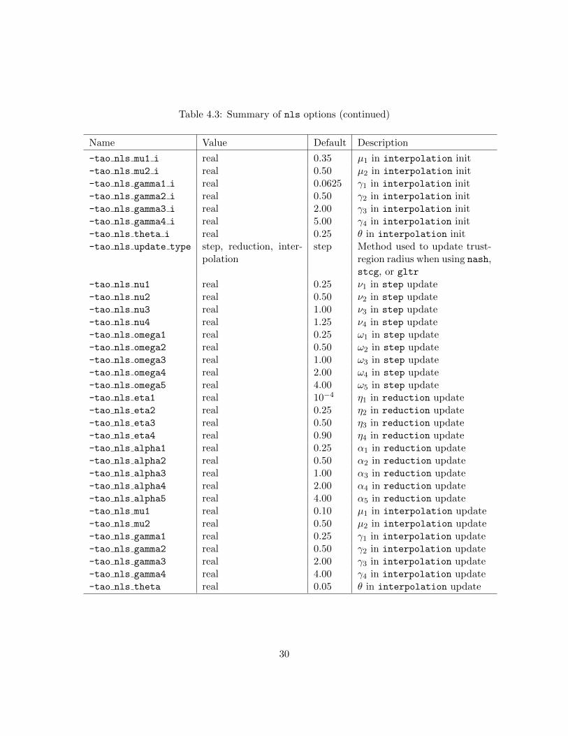
Table 4.3: Summary of nls options (continued)

Name Value Default Description

-tao nls mu1 i real 0.35 µ1 in interpolation init-tao nls mu2 i real 0.50 µ2 in interpolation init-tao nls gamma1 i real 0.0625 γ1 in interpolation init-tao nls gamma2 i real 0.50 γ2 in interpolation init-tao nls gamma3 i real 2.00 γ3 in interpolation init-tao nls gamma4 i real 5.00 γ4 in interpolation init-tao nls theta i real 0.25 θ in interpolation init-tao nls update type step, reduction, inter-

polationstep Method used to update trust-

region radius when using nash,stcg, or gltr

-tao nls nu1 real 0.25 ν1 in step update-tao nls nu2 real 0.50 ν2 in step update-tao nls nu3 real 1.00 ν3 in step update-tao nls nu4 real 1.25 ν4 in step update-tao nls omega1 real 0.25 ω1 in step update-tao nls omega2 real 0.50 ω2 in step update-tao nls omega3 real 1.00 ω3 in step update-tao nls omega4 real 2.00 ω4 in step update-tao nls omega5 real 4.00 ω5 in step update-tao nls eta1 real 10−4 η1 in reduction update-tao nls eta2 real 0.25 η2 in reduction update-tao nls eta3 real 0.50 η3 in reduction update-tao nls eta4 real 0.90 η4 in reduction update-tao nls alpha1 real 0.25 α1 in reduction update-tao nls alpha2 real 0.50 α2 in reduction update-tao nls alpha3 real 1.00 α3 in reduction update-tao nls alpha4 real 2.00 α4 in reduction update-tao nls alpha5 real 4.00 α5 in reduction update-tao nls mu1 real 0.10 µ1 in interpolation update-tao nls mu2 real 0.50 µ2 in interpolation update-tao nls gamma1 real 0.25 γ1 in interpolation update-tao nls gamma2 real 0.50 γ2 in interpolation update-tao nls gamma3 real 2.00 γ3 in interpolation update-tao nls gamma4 real 4.00 γ4 in interpolation update-tao nls theta real 0.05 θ in interpolation update

30

A good preconditioner reduces the number of iterations required to solve the linearsystem of equations. For the conjugate gradient methods and generalized Lanczos method,this preconditioner must be symmetric and positive definite. The available options are touse no preconditioner, the absolute value of the diagonal of the Hessian matrix, a limited-memory BFGS approximation to the Hessian matrix, or one of the other preconditionersprovided by the PETSc package. These preconditioners are specified by the command linearguments -tao nls pc type <none,ahess,bfgs,petsc>, respectively. The default is thebfgs preconditioner. When the preconditioner type is set to petsc, the preconditionerset with the PETSc -pc type command line argument is used. For example, to use anincomplete Cholesky factorization for the preconditioner, one would use the command linearguments -tao nls pc type petsc -pc type icc. See the PETSc manual for furtherinformation on changing the behavior of the preconditioners.

The choice of scaling matrix can significantly affect the quality of the Hessian approxi-mation when using the bfgs preconditioner and affect the number of iterations required bythe linear system solver. The choices for scaling matrices are the same as those discussed forthe limited-memory, variable-metric algorithm. For Newton methods, however, the optionexists to use a scaling matrix based on the true Hessian matrix. In particular, the imple-mentation supports using the absolute value of the diagonal of either the Hessian matrixor the perturbed Hessian matrix. The scaling matrix to use with the bfgs preconditioneris set with the command line argument -tao nls bfgs scale type <bfgs,ahess,phess>;phess is the default. The bfgs scaling matrix is derived from the BFGS options. The ahessscaling matrix is the absolute value of the diagonal of the Hessian matrix. The phess scalingmatrix is the absolute value of the diagonal of the perturbed Hessian matrix.

The perturbation ρk is added when the direction returned by the Krylov subspacemethod is not a descent direction, the Krylov method diverged due to an indefinite precondi-tioner or matrix, or a direction of negative curvature was found. In the last two cases, if thestep returned is a descent direction, it is used during the line search. Otherwise, a steepestdescent direction is used during the line search. The perturbation is decreased as long as theKrylov subspace method reports success and increased if further problems are encountered.There are three cases: initializing, increasing, and decreasing the perturbation. These casesare described below.

1. If ρk is zero and a problem was detected with either the direction or the Krylovsubspace method, the perturbation is initialized to

ρk+1 = median {imin, imfac ∗ ‖g(xk)‖, imax} ,

where g(xk) is the gradient of the objective function and imin is set with the com-mand line argument -tao nls imin <real> with a default value of 10−4, imfac by-tao nls imfac with a default value of 0.1, and imax by -tao nls imax with a de-fault value of 100. When using the gltr method to solve the system of equations, anestimate of the minimum eigenvalue λ1 of the Hessian matrix is available. This valueis used to initialize the perturbation to ρk+1 = max {ρk+1,−λ1} in this case.

2. If ρk is nonzero and a problem was detected with either the direction or Krylovsubspace method, the perturbation is increased to

ρk+1 = min {pmax,max {pgfac ∗ ρk, pmgfac ∗ ‖g(xk)‖}} ,

31

where g(xk) is the gradient of the objective function and pgfac is set with the com-mand line argument -tao nls pgfac with a default value of 10, pmgfac by -tao nls pmgfac

with a default value of 0.1, and pmax by -tao nls pmax with a default value of 100.

3. If ρk is nonzero and no problems were detected with either the direction or Krylovsubspace method, the perturbation is decreased to

ρk+1 = min {psfac ∗ ρk,pmsfac ∗ ‖g(xk)‖} ,

where g(xk) is the gradient of the objective function, psfac is set with the commandline argument -tao nls psfac with a default value of 0.4, and pmsfac is set by-tao nls pmsfac with a default value of 0.1. Moreover, if ρk+1 < pmin, then ρk+1 =0, where pmin is set with the command line argument -tao nls pmin and has a defaultvalue of 10−12.

Near a local minimizer to the unconstrained optimization problem, the Hessian matrix willbe positive-semidefinite; the perturbation will shrink toward zero, and one would eventuallyobserve a superlinear convergence rate.

When using nash, stcg, or gltr to solve the linear systems of equation, a trust-regionradius needs to be initialized and updated. This trust-region radius simultaneously limitsthe size of the step computed and reduces the number of iterations of the conjugate gradientmethod. The method for initializing the trust-region radius is set with the command lineargument -tao nls init type <constant,direction,interpolation>; interpolation,which chooses an initial value based on the interpolation scheme found in [6], is the default.This scheme performs a number of function and gradient evaluations to determine a radiussuch that the reduction predicted by the quadratic model along the gradient directioncoincides with the actual reduction in the nonlinear function. The iterate obtaining the bestobjective function value is used as the starting point for the main line search algorithm.The constant method initializes the trust-region radius by using the value specified withthe -tao trust0 <real> command line argument, where the default value is 100. Thedirection technique solves the first quadratic optimization problem by using a standardconjugate gradient method and initializes the trust region to ‖s0‖.

The method for updating the trust-region radius is set with the command line argument-tao nls update type <step,reduction,interpolation>; step is the default. The stepmethod updates the trust-region radius based on the value of τk. In particular,

∆k+1 =

ω1min(∆k, ‖dk‖) if τk ∈ [0, ν1)ω2min(∆k, ‖dk‖) if τk ∈ [ν1, ν2)ω3∆k if τk ∈ [ν2, ν3)max(∆k, ω4‖dk‖) if τk ∈ [ν3, ν4)max(∆k, ω5‖dk‖) if τk ∈ [ν4,∞),

where 0 < ω1 < ω2 < ω3 = 1 < ω4 < ω5 and 0 < ν1 < ν2 < ν3 < ν4 are constants. Thereduction method computes the ratio of the actual reduction in the objective function tothe reduction predicted by the quadratic model for the full step, κk = f(xk)−f(xk+dk)

q(xk)−q(xk+dk) , where

32

qk is the quadratic model. The radius is then updated as

∆k+1 =

α1min(∆k, ‖dk‖) if κk ∈ (−∞, η1)α2min(∆k, ‖dk‖) if κk ∈ [η1, η2)α3∆k if κk ∈ [η2, η3)max(∆k, α4‖dk‖) if κk ∈ [η3, η4)max(∆k, α5‖dk‖) if κk ∈ [η4,∞),

where 0 < α1 < α2 < α3 = 1 < α4 < α5 and 0 < η1 < η2 < η3 < η4 are constants. Theinterpolation method uses the same interpolation mechanism as in the initialization tocompute a new value for the trust-region radius.

4.1.5 Newton Trust-Region Method

The Newton trust-region method solves the constrained quadratic programming problem

mind12d

THkd+ gTk dsubject to ‖d‖ ≤ ∆k

to obtain a direction dk, where Hk is the Hessian of the objective function at xk, gk isthe gradient of the objective function at xk, and ∆k is the trust-region radius. If xk + dksufficiently reduces the nonlinear objective function, then the step is accepted, and the trust-region radius is updated. However, if xk + dk does not sufficiently reduce the nonlinearobjective function, then the step is rejected, the trust-region radius is reduced, and thequadratic program is re-solved by using the updated trust-region radius. The Newtontrust-region method can be set by using the TAO solver tao ntr. The options available forthis solver are listed in Table 4.4. For the best efficiency, function and gradient evaluationsshould be performed separately when using this algorithm.

The quadratic optimization problem is approximately solved by applying the Nash orSteihaug-Toint conjugate gradient methods or the generalized Lanczos method to the sym-metric system of equations Hkd = −gk. The method used to solve the system of equationsis specified with the command line argument -tao ntr ksp type <nash,stcg,gltr>; stcgis the default. Internally, the PETSc implementations for the Nash method, Steihaug-Tointmethod, and the generalized Lanczos method are used. See the PETSc manual for furtherinformation on changing the behavior of these linear system solvers.

A good preconditioner reduces the number of iterations required to compute the direc-tion. For the Nash and Steihaug-Toint conjugate gradient methods and generalized Lanczosmethod, this preconditioner must be symmetric and positive definite. The available optionsare to use no preconditioner, the absolute value of the diagonal of the Hessian matrix,a limited-memory BFGS approximation to the Hessian matrix, or one of the other pre-conditioners provided by the PETSc package. These preconditioners are specified by thecommand line argument -tao ntr pc type <none,ahess,bfgs,petsc>, respectively. Thedefault is the bfgs preconditioner. When the preconditioner type is set to petsc, the pre-conditioner set with the PETSc -pc type command line argument is used. For example,to use an incomplete Cholesky factorization for the preconditioner, one would use the com-mand line arguments -tao ntr pc type petsc -pc type icc. See the PETSc manual forfurther information on changing the behavior of the preconditioners.

33

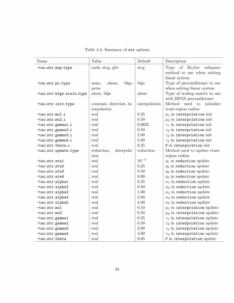
Table 4.4: Summary of ntr options

Name Value Default Description

-tao ntr ksp type nash, stcg, gltr stcg Type of Krylov subspacemethod to use when solvinglinear system

-tao ntr pc type none, ahess, bfgs,petsc

bfgs Type of preconditioner to usewhen solving linear system

-tao ntr bfgs scale type ahess, bfgs ahess Type of scaling matrix to usewith BFGS preconditioner

-tao ntr init type constant, direction, in-terpolation

interpolation Method used to initializetrust-region radius

-tao ntr mu1 i real 0.35 µ1 in interpolation init-tao ntr mu2 i real 0.50 µ2 in interpolation init-tao ntr gamma1 i real 0.0625 γ1 in interpolation init-tao ntr gamma2 i real 0.50 γ2 in interpolation init-tao ntr gamma3 i real 2.00 γ3 in interpolation init-tao ntr gamma4 i real 5.00 γ4 in interpolation init-tao ntr theta i real 0.25 θ in interpolation init-tao ntr update type reduction, interpola-

tionreduction Method used to update trust-

region radius-tao ntr eta1 real 10−4 η1 in reduction update-tao ntr eta2 real 0.25 η2 in reduction update-tao ntr eta3 real 0.50 η3 in reduction update-tao ntr eta4 real 0.90 η4 in reduction update-tao ntr alpha1 real 0.25 α1 in reduction update-tao ntr alpha2 real 0.50 α2 in reduction update-tao ntr alpha3 real 1.00 α3 in reduction update-tao ntr alpha4 real 2.00 α4 in reduction update-tao ntr alpha5 real 4.00 α5 in reduction update-tao ntr mu1 real 0.10 µ1 in interpolation update-tao ntr mu2 real 0.50 µ2 in interpolation update-tao ntr gamma1 real 0.25 γ1 in interpolation update-tao ntr gamma2 real 0.50 γ2 in interpolation update-tao ntr gamma3 real 2.00 γ3 in interpolation update-tao ntr gamma4 real 4.00 γ4 in interpolation update-tao ntr theta real 0.05 θ in interpolation update

34

The choice of scaling matrix can significantly affect the quality of the Hessian approxi-mation when using the bfgs preconditioner and affect the number of iterations required bythe linear system solver. The choices for scaling matrices are the same as those discussed forthe limited-memory, variable-metric algorithm. For Newton methods, however, the optionexists to use a scaling matrix based on the true Hessian matrix. In particular, the imple-mentation supports using the absolute value of the diagonal of the Hessian matrix. Thescaling matrix to use with the bfgs preconditioner is set with the command line arguments-tao ntr bfgs scale type <ahess,bfgs>; ahess is the default. The bfgs scaling matrixis derived from the BFGS options. The ahess scaling matrix is the absolute value of thediagonal of the Hessian matrix.

The method for computing an initial trust-region radius is set with the command line ar-guments -tao ntr init type <constant,direction,interpolation>; interpolation,which chooses an initial value based on the interpolation scheme found in [6], is the de-fault. This scheme performs a number of function and gradient evaluations to determine aradius such that the reduction predicted by the quadratic model along the gradient directioncoincides with the actual reduction in the nonlinear function. The iterate obtaining the bestobjective function value is used as the starting point for the main trust-region algorithm.The constant method initializes the trust-region radius by using the value specified withthe -tao trust0 <real> command line argument, where the default value is 100. Thedirection technique solves the first quadratic optimization problem by using a standardconjugate gradient method and initializes the trust region to ‖s0‖.

The method for updating the trust-region radius is set with the command line ar-guments -tao ntr update type <reduction,interpolation>; reduction is the default.The reduction method computes the ratio of the actual reduction in the objective functionto the reduction predicted by the quadratic model for the full step, κk = f(xk)−f(xk+dk)

q(xk)−q(xk+dk) ,where qk is the quadratic model. The radius is then updated as

∆k+1 =

α1min(∆k, ‖dk‖) if κk ∈ (−∞, η1)α2min(∆k, ‖dk‖) if κk ∈ [η1, η2)α3∆k if κk ∈ [η2, η3)max(∆k, α4‖dk‖) if κk ∈ [η3, η4)max(∆k, α5‖dk‖) if κk ∈ [η4,∞),

where 0 < α1 < α2 < α3 = 1 < α4 < α5 and 0 < η1 < η2 < η3 < η4 are constants. Theinterpolation method uses the same interpolation mechanism as in the initialization tocompute a new value for the trust-region radius.

4.1.6 BMRM

The Bundle Method for Regularized Risk Minimization (BMRM)[?] is a numerical approachto optimizing an unconstrained objective in the form of f(x) + 0.5 ∗ λ‖x‖2. Here f is aconvex function that is finite on the whole space. λ is a positive weight parameter, and‖x‖ is the Euclidean norm of x. The algorithm only requires a routine which, given an x,returns the value of f(x) and the gradient of f at x.

35

4.1.7 OWL-QN

The Orthant-Wise Limited-memory Quasi-Newton algorithm (OWL-QN)[1] is a numericalapproach to optimizing an unconstrained objective in the form of f(x) + λ‖x‖1. Here f isa convex and differentiable function, λ is a positive weight parameter, and ‖x‖1 is the L1norm of x:

∑i |xi|. The algorithm only requires evaluating the value of f and its gradient.

4.2 Bound-Constrained Optimization

Bound-constrained optimization algorithms minimize f : Rn → R, subject to upper orlower bounds on some of the variables. These solvers use the bounds on the variables aswell as objective function, gradient, and possibly Hessian information.

4.2.1 Projected Gradient Descent Method

PGD is a steepest descent algorithm with projected gradients and a bounded More-Thuenteline search. The method can be set by using the TAO solver TAO PGD or the -tao type pgd

flag, and serves as a useful worst-case benchmarking tool when developing more advancedbound-constrained algorithms.

4.2.2 Bounded Nonlinear Conjugate Gradient

BNCG extends the unconstrained nonlinear conjugate gradient algorithm to bound con-straints via gradient projections and a bounded More-Thuente line search. Like its un-constrained counterpart, BNCG offers a variety of CG updates: Fletched-Reeves, Polak-Ribiere, Polak-Ribiere-Plus, Hestenes-Stiefel, and the Dai-Yuan. These conjugate gra-dient methods can be specified by using the command line argument -tao bncg type

<fr,pr,prp,hs,dy>, respectively. The default value is dy. BNCS is available via theTAO solver TAO BNCG or the -tao type bncg flag.

In addition to automatic restarts under orthogonality conditions, BNCG also featuresselective step restarts for previously active bounds that become inactive at a new iterate,and a weak check on descent direction such that∇f(xk)

Tdk ≤ −ρ||dk||p. Parameters for thisweak check have default values of ρ = 10−4 and p = 2.1, respectively, and can be modifiedusing -tao bncg rho and -tao bncg pow flags. Finally, the default orthogonality tolerancehas been slightly relaxed compared to the unconstrained version to improve convergence.

4.2.3 Trust-Region Newton Method

The TRON [20] algorithm is an active-set method that uses a combination of gradient pro-jections and a preconditioned conjugate gradient method to minimize an objective function.Each iteration of the TRON algorithm requires function, gradient, and Hessian evaluations.In each iteration, the algorithm first applies several conjugate gradient iterations. Afterthese iterates, the TRON solver momentarily ignores the variables that equal one of itsbounds and applies a preconditioned conjugate gradient method to a quadratic model ofthe remaining set of “free” variables.

36

The TRON algorithm solves a reduced linear system defined by the rows and columnscorresponding to the variables that lie between the upper and lower bounds. The TRONalgorithm applies a trust region to the conjugate gradients to ensure convergence. Theinitial trust-region radius can be set by using the command TaoSetInitialTrustRegion-

Radius(), and the current trust region size can be found by using the command TaoGet-

CurrentTrustRegionRadius(). The initial trust region can significantly alter the rate ofconvergence for the algorithm and should be tuned and adjusted for optimal performance.

4.2.4 Gradient Projection Conjugate Gradient Method

The GPCG [23] algorithm is much like the TRON algorithm, discussed in Section 4.2.3,except that it assumes that the objective function is quadratic and convex. Therefore, itevaluates the function, gradient, and Hessian only once. Since the objective function isquadratic, the algorithm does not use a trust region. All the options that apply to TRONexcept for trust-region options also apply to GPCG.

4.2.5 Interior-Point Newton’s Method

The BQPIP algorithm is an interior-point method for bound constrained quadratic op-timization. It can be set by using the TAO solver of tao bqpip. Since it assumes theobjective function is quadratic, it evaluates the function, gradient, and Hessian only once.This method also requires the solution of systems of linear equations, whose solver can beaccessed and modified with the command TaoGetKSP().

4.2.6 Bound-constrained Limited-Memory Variable-Metric Method

BLMVM is a limited-memory, variable-metric method and is the bound-constrained vari-ant of the LMVM method for unconstrained optimization. It uses projected gradients toapproximate the Hessian, eliminating the need for Hessian evaluations. The method can beset by using the TAO solver tao blmvm. The command TaoLMVMSetSize(), which sets thenumber of vectors to be used in the Hessian approximation, also applies to this method.

4.3 PDE-Constrained Optimization

TAO solves PDE-constrained optimization problems of the form

minu,v

f(u, v)

subject to g(u, v) = 0,

where the state variable u is the solution to the discretized partial differential equationdefined by g and parametrized by the design variable v, and f is an objective function. TheLagrange multipliers on the constraint are denoted by y. This method is set by using thelinearly constrained augmented Lagrangian TAO solver tao lcl.

We make two main assumptions when solving these problems: the objective functionand PDE constraints have been discretized so that we can treat the optimization problemas finite dimensional and ∇ug(u, v) is invertible for all u and v.

37

4.3.1 Linearly-Constrained Augmented Lagrangian Method

Given the current iterate (uk, vk, yk), the linearly constrained augmented Lagrangian methodapproximately solves the optimization problem

minu,v

fk(u, v)

subject to Ak(u− uk) +Bk(v − vk) + gk = 0,

where Ak = ∇ug(uk, vk), Bk = ∇vg(uk, vk), and gk = g(uk, vk) and

fk(u, v) = f(u, v)− g(u, v)T yk +ρk2‖g(u, v)‖2

is the augmented Lagrangian function. This optimization problem is solved in two stages.The first computes the Newton direction and finds a feasible point for the linear constraints.The second computes a reduced-space direction that maintains feasibility with respect tothe linearized constraints and improves the augmented Lagrangian merit function.

Newton Step

The Newton direction is obtained by fixing the design variables at their current value andsolving the linearized constraint for the state variables. In particular, we solve the systemof equations

Akdu = −gkto obtain a direction du. We need a direction that provides sufficient descent for the meritfunction

1

2‖g(u, v)‖2.

That is, we require gTk Akdu < 0.If the Newton direction is a descent direction, then we choose a penalty parameter ρk so

that du is also a sufficient descent direction for the augmented Lagrangian merit function.We then find α to approximately minimize the augmented Lagrangian merit function alongthe Newton direction.

minα≥0

fk(uk + αdu, vk).

We can enforce either the sufficient decrease condition or the Wolfe conditions during thesearch procedure. The new point,

uk+ 12

= uk + αkdu

vk+ 12

= vk,

satisfies the linear constraint

Ak(uk+ 12− uk) +Bk(vk+ 1

2− vk) + αkgk = 0.

If the Newton direction computed does not provide descent for the merit function, then wecan use the steepest descent direction du = −ATk gk during the search procedure. However,the implication that the intermediate point approximately satisfies the linear constraint isno longer true.

38

Modified Reduced-Space Step

We are now ready to compute a reduced-space step for the modified optimization problem:

minu,v

fk(u, v)

subject to Ak(u− uk) +Bk(v − vk) + αkgk = 0.

We begin with the change of variables

mindu,dv

fk(uk + du, vk + dv)

subject to Akdu+Bkdv + αkgk = 0

and make the substitutiondu = −A−1

k (Bkdv + αkgk).

Hence, the unconstrained optimization problem we need to solve is

mindv

fk(uk −A−1k (Bkdv + αkgk), vk + dv),

which is equivalent to

mindv

fk(uk+ 12−A−1

k Bkdv, vk+ 12

+ dv).

We apply one step of a limited-memory quasi-Newton method to this problem. The directionis obtain by solving the quadratic problem

mindv

12dv

T Hkdv + gTk+ 1

2

dv,

where Hk is the limited-memory quasi-Newton approximation to the reduced Hessian ma-trix, a positive-definite matrix, and gk+ 1

2is the reduced gradient.

gk+ 12

= ∇vfk(uk+ 12, vk+ 1

2)−∇ufk(uk+ 1

2, vk+ 1

2)A−1

k Bk

= dk+ 12

+ ck+ 12A−1k Bk

The reduced gradient is obtained from one linearized adjoint solve

yk+ 12

= A−Tk ck+ 1

2

and some linear algebragk+ 1

2= dk+ 1

2+ yT

k+ 12

Bk.

Because the Hessian approximation is positive definite and we know its inverse, we obtainthe direction

dv = −H−1k gk+ 1

2

and recover the full-space direction from one linearized forward solve,

du = −A−1k Bkdv.

39

Having the full-space direction, which satisfies the linear constraint, we now approximatelyminimize the augmented Lagrangian merit function along the direction.

minβ≥0

fk(uk+ 12

+ βdu, vk+ 12

+ βdv)

We enforce the Wolfe conditions during the search procedure. The new point is

uk+1 = uk+ 12

+ βkdu

vk+1 = vk+ 12

+ βkdv.

The reduced gradient at the new point is computed from

yk+1 = A−Tk ck+1

gk+1 = dk+1 − yTk+1Bk,

where ck+1 = ∇ufk(uk+1, vk+1) and dk+1 = ∇vfk(uk+1, vk+1). The multipliers yk+1 becomethe multipliers used in the next iteration of the code. The quantities vk+ 1

2, vk+1, gk+ 1

2, and

gk+1 are used to update Hk to obtain the limited-memory quasi-Newton approximation tothe reduced Hessian matrix used in the next iteration of the code. The update is skippedif it cannot be performed.

4.4 Nonlinear Least-Squares

Given a function F : Rn → Rm, the nonlinear least-squares problem minimizes

f(x) = ‖F (x)‖22 =

m∑i=1

Fi(x)2. (4.1)

The nonlinear equations F should be specified with the function TaoSetSeparableObjective-

Function(). Although the current version of TAO has no derivative-based algorithms fornonlinear least squares, we anticipate that such an algorithm will be available in the nextrelease.

4.4.1 POUNDerS

One algorithm for solving the least squares problem (4.1) when the Jacobian of the resid-ual vector F is unavailable is the model-based POUNDerS (Practical Optimization UsingNo Derivatives for sums of Squares) algorithm (tao pounders). POUNDerS employs aderivative-free trust-region framework as described in [7] in order to converge to local min-imizers. An example of this version of POUNDerS applied to a practical least-squaresproblem can be found in [18].

Derivative-Free Trust-Region Algorithm

In each iteration k, the algorithm maintains a model mk(x), described below, of the non-linear least squares function f centered about the current iterate xk.

40

If one assumes that the maximum number of function evaluations has not been reachedand that ‖∇mk(xk)‖2 >gtol, the next point x+ to be evaluated is obtained by solving thetrust-region subproblem

min {mk(x) : ‖x− xk‖p ≤ ∆k, } , (4.2)

where ∆k is the current trust-region radius. By default we use a trust-region norm withp = ∞ and solve (4.2) with the BLMVM method described in Section 4.2.6. While thesubproblem is a bound-constrained quadratic program, it may not be convex and the BQPIPand GPCG methods may not solve the subproblem. Therefore, either BLMVM (the default)or TRON should be used. Note: TRON uses its own internal trust region that may interferewith the infinity-norm trust region used in the model problem (4.2).

The residual vector is then evaluated to obtain F (x+) and hence f(x+). The ratio ofactual decrease to predicted decrease,

ρk =f(xk)− f(x+)

mk(xk)−mk(x+),

as well as an indicator, valid, on the model’s quality of approximation on the trust regionis then used to update the iterate,

xk+1 =

x+ if ρk ≥ η1x+ if 0 < ρk < η1 and valid=true

xk else,

and trust-region radius,

∆k+1 =

min(γ1∆k,∆max) if ρk ≥ η1 and ‖x+ − xk‖p ≥ ω1∆k

γ0∆k if ρk < η1 and valid=true

∆k else,

where 0 < η1 < 1, 0 < γ0 < 1 < γ1, 0 < ω1 < 1, and ∆max are constants.If ρk ≤ 0 and valid is false, the iterate and trust-region radius remain unchanged

after the above updates, and the algorithm tests whether the direction x+ − xk improvesthe model. If not, the algorithm performs an additional evaluation to obtain F (xk + dk),where dk is a model-improving direction.

The iteration counter is then updated, and the next model mk is obtained as describednext.

Forming the Trust-Region Model

In each iteration, POUNDerS uses a subset of the available evaluated residual vectors{F (y1), F (y2), · · ·} to form an interpolatory quadratic model of each residual component.The m quadratic models

q(i)k (x) = Fi(xk) + (x− xk)T g

(i)k +

1

2(x− xk)TH

(i)k (x− xk), i = 1, . . . ,m (4.3)

thus satisfy the interpolation conditions

q(i)k (yj) = Fi(yj), i = 1, . . . ,m; j = 1, . . . , lk

41

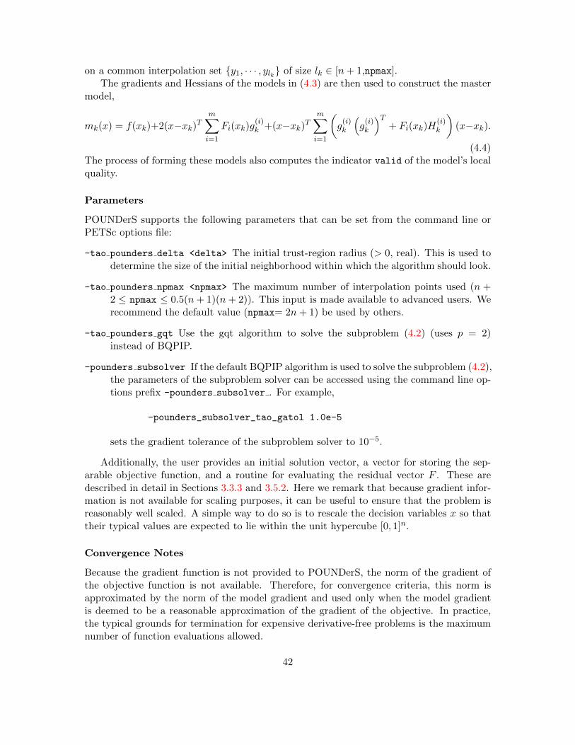
on a common interpolation set {y1, · · · , ylk} of size lk ∈ [n+ 1,npmax].The gradients and Hessians of the models in (4.3) are then used to construct the master

model,

mk(x) = f(xk)+2(x−xk)Tm∑i=1

Fi(xk)g(i)k +(x−xk)T

m∑i=1

(g(i)k

(g(i)k

)T+ Fi(xk)H

(i)k

)(x−xk).

(4.4)The process of forming these models also computes the indicator valid of the model’s localquality.

Parameters

POUNDerS supports the following parameters that can be set from the command line orPETSc options file:

-tao pounders delta <delta> The initial trust-region radius (> 0, real). This is used todetermine the size of the initial neighborhood within which the algorithm should look.

-tao pounders npmax <npmax> The maximum number of interpolation points used (n +2 ≤ npmax ≤ 0.5(n+ 1)(n+ 2)). This input is made available to advanced users. Werecommend the default value (npmax= 2n+ 1) be used by others.

-tao pounders gqt Use the gqt algorithm to solve the subproblem (4.2) (uses p = 2)instead of BQPIP.

-pounders subsolver If the default BQPIP algorithm is used to solve the subproblem (4.2),the parameters of the subproblem solver can be accessed using the command line op-tions prefix -pounders subsolver . For example,

-pounders_subsolver_tao_gatol 1.0e-5

sets the gradient tolerance of the subproblem solver to 10−5.

Additionally, the user provides an initial solution vector, a vector for storing the sep-arable objective function, and a routine for evaluating the residual vector F . These aredescribed in detail in Sections 3.3.3 and 3.5.2. Here we remark that because gradient infor-mation is not available for scaling purposes, it can be useful to ensure that the problem isreasonably well scaled. A simple way to do so is to rescale the decision variables x so thattheir typical values are expected to lie within the unit hypercube [0, 1]n.

Convergence Notes

Because the gradient function is not provided to POUNDerS, the norm of the gradient ofthe objective function is not available. Therefore, for convergence criteria, this norm isapproximated by the norm of the model gradient and used only when the model gradientis deemed to be a reasonable approximation of the gradient of the objective. In practice,the typical grounds for termination for expensive derivative-free problems is the maximumnumber of function evaluations allowed.

42

4.5 Complementarity

Mixed complementarity problems, or box-constrained variational inequalities, are related tononlinear systems of equations. They are defined by a continuously differentiable function,F : Rn → Rn, and bounds, ` ∈ {R ∪ {−∞}}n and u ∈ {R ∪ {∞}}n, on the variables suchthat ` ≤ u. Given this information, x∗ ∈ [`, u] is a solution to MCP(F , `, u) if for eachi ∈ {1, . . . , n} we have at least one of the following:

Fi(x∗) ≥ 0 if x∗i = `i

Fi(x∗) = 0 if `i < x∗i < ui

Fi(x∗) ≤ 0 if x∗i = ui.

Note that when ` = {−∞}n and u = {∞}n, we have a nonlinear system of equations, and` = {0}n and u = {∞}n correspond to the nonlinear complementarity problem [8].

Simple complementarity conditions arise from the first-order optimality conditions fromoptimization [17, 19]. In the simple bound-constrained optimization case, these conditionscorrespond to MCP(∇f , `, u), where f : Rn → R is the objective function. In a one-dimensional setting these conditions are intuitive. If the solution is at the lower bound,then the function must be increasing and ∇f ≥ 0. If the solution is at the upper bound,then the function must be decreasing and ∇f ≤ 0. If the solution is strictly between thebounds, we must be at a stationary point and ∇f = 0. Other complementarity problemsarise in economics and engineering [11], game theory [25], and finance [16].

Evaluation routines for F and its Jacobian must be supplied prior to solving the appli-cation. The bounds, [`, u], on the variables must also be provided. If no starting point issupplied, a default starting point of all zeros is used.

4.5.1 Semismooth Methods

TAO has two implementations of semismooth algorithms [24, 9, 10] for solving mixed com-plementarity problems. Both are based on a reformulation of the mixed complementarityproblem as a nonsmooth system of equations using the Fischer-Burmeister function [12]. Anonsmooth Newton method is applied to the reformulated system to calculate a solution.The theoretical properties of such methods are detailed in the aforementioned references.

The Fischer-Burmeister function, φ : R2 → R, is defined as

φ(a, b) :=√a2 + b2 − a− b.

This function has the following key property,

φ(a, b) = 0 ⇔ a ≥ 0, b ≥ 0, ab = 0,

used when reformulating the mixed complementarity problem as the system of equationsΦ(x) = 0, where Φ : Rn → Rn. The reformulation is defined componentwise as

Φi(x) :=

φ(xi − li, Fi(x)) if −∞ < li < ui =∞,−φ(ui − xi,−Fi(x)) if −∞ = li < ui <∞,φ(xi − li, φ(ui − xi,−Fi(x))) if −∞ < li < ui <∞,−Fi(x) if −∞ = li < ui =∞,li − xi if −∞ < li = ui <∞.

43

We note that Φ is not differentiable everywhere but satisfies a semismoothness property[21, 28, 29]. Furthermore, the natural merit function, Ψ(x) := 1

2‖Φ(x)‖22, is continuouslydifferentiable.

The two semismooth TAO solvers both solve the system Φ(x) = 0 by applying a non-smooth Newton method with a line search. We calculate a direction, dk, by solving thesystem Hkdk = −Φ(xk), where Hk is an element of the B-subdifferential [29] of Φ at xk. Ifthe direction calculated does not satisfy a suitable descent condition, then we use the neg-ative gradient of the merit function, −∇Ψ(xk), as the search direction. A standard Armijosearch [2] is used to find the new iteration. Nonmonotone searches [14] are also availableby setting appropriate runtime options. See Section 5.4 for further details.

The first semismooth algorithm available in TAO is not guaranteed to remain feasiblewith respect to the bounds, [`, u], and is termed an infeasible semismooth method. Thismethod can be specified by using the tao ssils solver. In this case, the descent test usedis that

∇Ψ(xk)Tdk ≤ −δ‖dk‖ρ.

Both δ > 0 and ρ > 2 can be modified by using the runtime options -tao ssils delta

<delta> and -tao ssils rho <rho>, respectively. By default, δ = 10−10 and ρ = 2.1.An alternative is to remain feasible with respect to the bounds by using a projected

Armijo line search. This method can be specified by using the tao ssfls solver. Thedescent test used is the same as above where the direction in this case corresponds to thefirst part of the piecewise linear arc searched by the projected line search. Both δ > 0and ρ > 2 can be modified by using the runtime options -tao ssfls delta <delta> and-tao ssfls rho <rho> respectively. By default, δ = 10−10 and ρ = 2.1.

The recommended algorithm is the infeasible semismooth method, tao ssils, becauseof its strong global and local convergence properties. However, if it is known that F isnot defined outside of the box, [`, u], perhaps because of the presence of log functions, thefeasibility-enforcing version of the algorithm, tao ssfls, is a reasonable alternative.

44

Chapter 5

Advanced Options

This section discusses options and routines that apply to most TAO solvers and problemclasses. In particular, we focus on linear solvers, convergence tests, and line searches.

5.1 Linear Solvers

One of the most computationally intensive phases of many optimization algorithms involvesthe solution of linear systems of equations. The performance of the linear solver may becritical to an efficient computation of the solution. Since linear equation solvers often havea wide variety of options associated with them, TAO allows the user to access the linearsolver with the

TaoGetKSP(Tao, KSP *);

command. With access to the KSP object, users can customize it for their application toachieve improved performance. Additional details on the KSP options in PETSc can befound in the PETSc users manual [5].

5.2 Monitors

By default the TAO solvers run silently without displaying information about the iterations.The user can initiate monitoring with the command

TaoSetMonitor(Tao,

PetscErrorCode (*mon)(Tao,void*),

void*);

The routine mon indicates a user-defined monitoring routine, and void* denotes an optionaluser-defined context for private data for the monitor routine.

The routine set by TaoSetMonitor() is called once during each iteration of the op-timization solver. Hence, the user can employ this routine for any application-specificcomputations that should be done after the solution update.

45

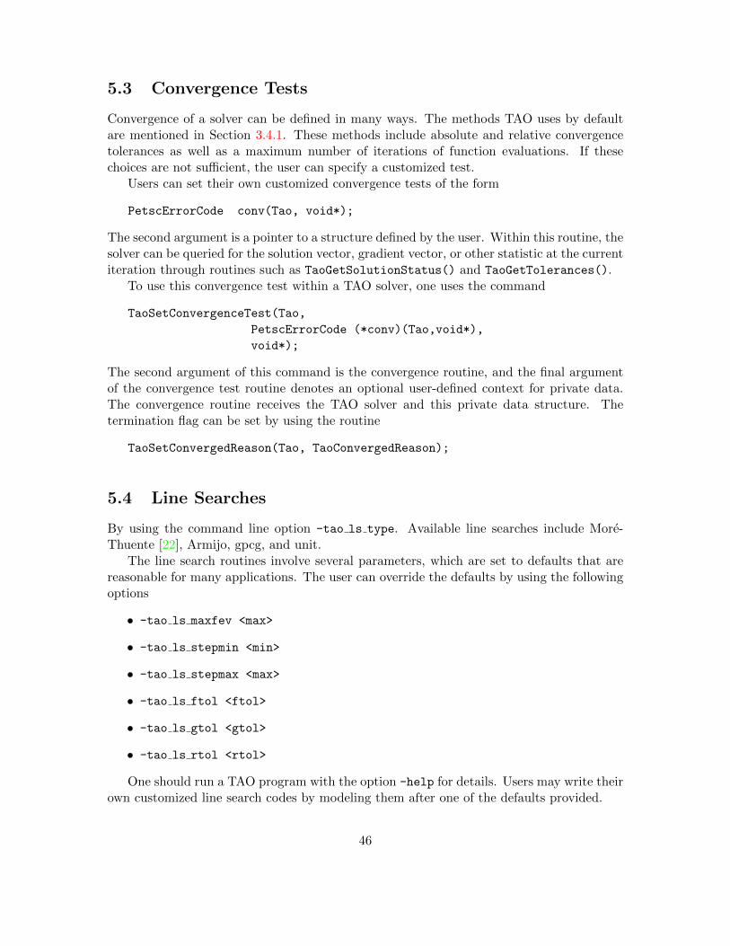
5.3 Convergence Tests

Convergence of a solver can be defined in many ways. The methods TAO uses by defaultare mentioned in Section 3.4.1. These methods include absolute and relative convergencetolerances as well as a maximum number of iterations of function evaluations. If thesechoices are not sufficient, the user can specify a customized test.

Users can set their own customized convergence tests of the form

PetscErrorCode conv(Tao, void*);

The second argument is a pointer to a structure defined by the user. Within this routine, thesolver can be queried for the solution vector, gradient vector, or other statistic at the currentiteration through routines such as TaoGetSolutionStatus() and TaoGetTolerances().

To use this convergence test within a TAO solver, one uses the command

TaoSetConvergenceTest(Tao,

PetscErrorCode (*conv)(Tao,void*),

void*);

The second argument of this command is the convergence routine, and the final argumentof the convergence test routine denotes an optional user-defined context for private data.The convergence routine receives the TAO solver and this private data structure. Thetermination flag can be set by using the routine

TaoSetConvergedReason(Tao, TaoConvergedReason);

5.4 Line Searches

By using the command line option -tao ls type. Available line searches include More-Thuente [22], Armijo, gpcg, and unit.

The line search routines involve several parameters, which are set to defaults that arereasonable for many applications. The user can override the defaults by using the followingoptions

• -tao ls maxfev <max>

• -tao ls stepmin <min>

• -tao ls stepmax <max>

• -tao ls ftol <ftol>

• -tao ls gtol <gtol>

• -tao ls rtol <rtol>

One should run a TAO program with the option -help for details. Users may write theirown customized line search codes by modeling them after one of the defaults provided.

46

Chapter 6

Adding a Solver

One of the strengths of both TAO and PETSc is the ability to allow users to extend thebuilt-in solvers with new user-defined algorithms. It is certainly possible to develop newoptimization algorithms outside of TAO framework, but Using TAO to implement a solverhas many advantages,

1. TAO includes other optimization solvers with an identical interface, so applicationproblems may conveniently switch solvers to compare their effectiveness.

2. TAO provides support for function evaluations and derivative information. It allowsfor the direct evaluation of this information by the application developer, containslimited support for finite difference approximations, and allows the uses of matrix-freemethods. The solvers can obtain this function and derivative information through asimple interface while the details of its computation are handled within the toolkit.

3. TAO provides line searches, convergence tests, monitoring routines, and other toolsthat are helpful in an optimization algorithm. The availability of these tools meansthat the developers of the optimization solver do not have to write these utilities.

4. PETSc offers vectors, matrices, index sets, and linear solvers that can be used bythe solver. These objects are standard mathematical constructions that have manydifferent implementations. The objects may be distributed over multiple processors,restricted to a single processor, have a dense representation, use a sparse data struc-ture, or vary in many other ways. TAO solvers do not need to know how these objectsare represented or how the operations defined on them have been implemented. In-stead, the solvers apply these operations through an abstract interface that leavesthe details to PETSc and external libraries. This abstraction allows solvers to workseamlessly with a variety of data structures while allowing application developers toselect data structures tailored for their purposes.

5. PETSc provides the user a convenient method for setting options at runtime, perfor-mance profiling, and debugging.

47

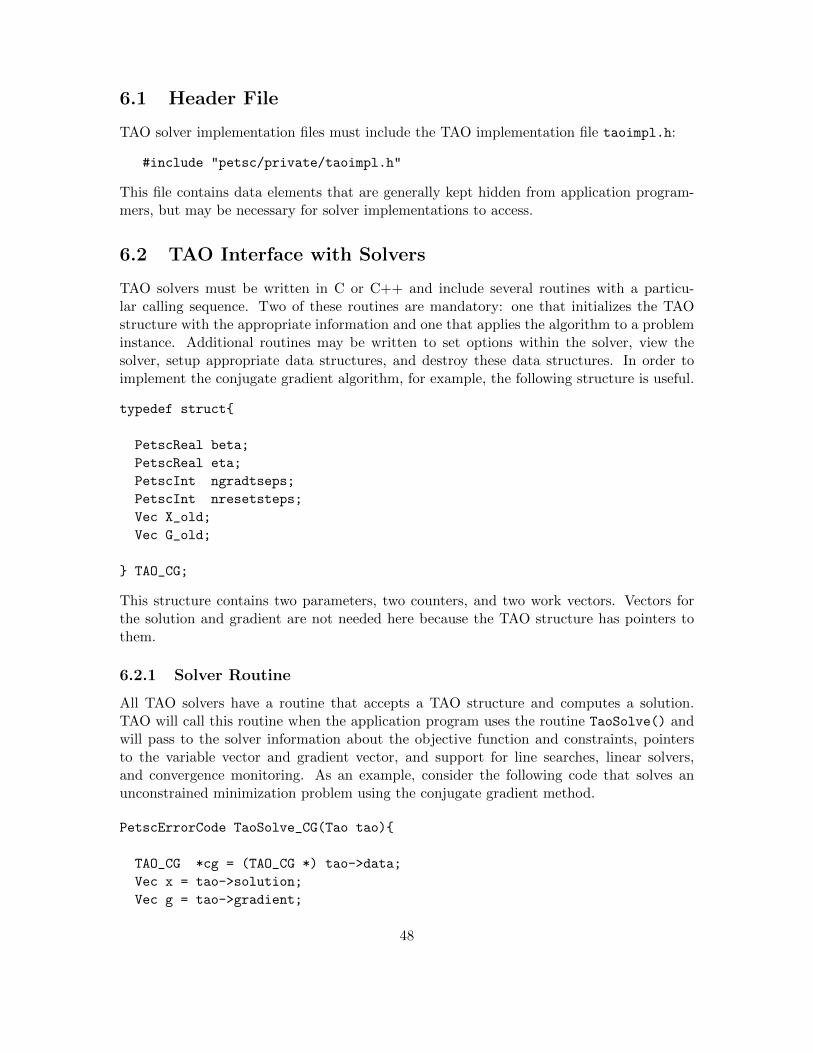
6.1 Header File

TAO solver implementation files must include the TAO implementation file taoimpl.h:

#include "petsc/private/taoimpl.h"

This file contains data elements that are generally kept hidden from application program-mers, but may be necessary for solver implementations to access.

6.2 TAO Interface with Solvers

TAO solvers must be written in C or C++ and include several routines with a particu-lar calling sequence. Two of these routines are mandatory: one that initializes the TAOstructure with the appropriate information and one that applies the algorithm to a probleminstance. Additional routines may be written to set options within the solver, view thesolver, setup appropriate data structures, and destroy these data structures. In order toimplement the conjugate gradient algorithm, for example, the following structure is useful.

typedef struct{

PetscReal beta;

PetscReal eta;

PetscInt ngradtseps;

PetscInt nresetsteps;

Vec X_old;

Vec G_old;

} TAO_CG;

This structure contains two parameters, two counters, and two work vectors. Vectors forthe solution and gradient are not needed here because the TAO structure has pointers tothem.

6.2.1 Solver Routine

All TAO solvers have a routine that accepts a TAO structure and computes a solution.TAO will call this routine when the application program uses the routine TaoSolve() andwill pass to the solver information about the objective function and constraints, pointersto the variable vector and gradient vector, and support for line searches, linear solvers,and convergence monitoring. As an example, consider the following code that solves anunconstrained minimization problem using the conjugate gradient method.

PetscErrorCode TaoSolve_CG(Tao tao){

TAO_CG *cg = (TAO_CG *) tao->data;

Vec x = tao->solution;

Vec g = tao->gradient;

48

Vec s = tao->stepdirection;

PetscInt iter=0;

PetscReal gnormPrev,gdx,f,gnorm,steplength=0;

TaoLineSearchConvergedReason lsflag=TAO_LINESEARCH_CONTINUE_ITERATING;

TaoConvergedReason reason=TAO_CONTINUE_ITERATING;

PetscErrorCode ierr;

PetscFunctionBegin;

ierr = TaoComputeObjectiveAndGradient(tao,x,&f,g);CHKERRQ(ierr);

ierr = VecNorm(g,NORM_2,&gnorm); CHKERRQ(ierr);

ierr = VecSet(s,0); CHKERRQ(ierr);

cg->beta=0;

gnormPrev = gnorm;

/* Enter loop */

while (1){

/* Test for convergence */

ierr = TaoMonitor(tao,iter,f,gnorm,0.0,step,&reason);CHKERRQ(ierr);

if (reason!=TAO_CONTINUE_ITERATING) break;

cg->beta=(gnorm*gnorm)/(gnormPrev*gnormPrev);

ierr = VecScale(s,cg->beta); CHKERRQ(ierr);

ierr = VecAXPY(s,-1.0,g); CHKERRQ(ierr);

ierr = VecDot(s,g,&gdx); CHKERRQ(ierr);

if (gdx>=0){ /* If not a descent direction, use gradient */

ierr = VecCopy(g,s); CHKERRQ(ierr);

ierr = VecScale(s,-1.0); CHKERRQ(ierr);

gdx=-gnorm*gnorm;

}

/* Line Search */

gnormPrev = gnorm; step=1.0;

ierr = TaoLineSearchSetInitialStepLength(tao->linesearch,1.0);

ierr = TaoLineSearchApply(tao->linesearch,x,&f,g,s,&steplength,&lsflag);

ierr = TaoAddLineSearchCounts(tao); CHKERRQ(ierr);

ierr = VecNorm(g,NORM_2,&gnorm);CHKERRQ(ierr);

iter++;

}

PetscFunctionReturn(0);

49

}

The first line of this routine casts the second argument to a pointer to a TAO CG datastructure. This structure contains pointers to three vectors and a scalar that will be neededin the algorithm.

After declaring an initializing several variables, the solver lets TAO evaluate the func-tion and gradient at the current point in the using the routine TaoComputeObjective-

AndGradient(). Other routines may be used to evaluate the Hessian matrix or evaluateconstraints. TAO may obtain this information using direct evaluation or other means, butthese details do not affect our implementation of the algorithm.

The norm of the gradient is a standard measure used by unconstrained minimizationsolvers to define convergence. This quantity is always nonnegative and equals zero at thesolution. The solver will pass this quantity, the current function value, the current iterationnumber, and a measure of infeasibility to TAO with the routine

PetscErrorCode TaoMonitor(Tao tao, PetscInt iter, PetscReal f,

PetscReal res, PetscReal cnorm, PetscReal steplength,

TaoConvergedReason *reason);

Most optimization algorithms are iterative, and solvers should include this command some-where in each iteration. This routine records this information, and applies any monitoringroutines and convergence tests set by default or the user. In this routine, the second argu-ment is the current iteration number, and the third argument is the current function value.The fourth argument is a nonnegative error measure associated with the distance betweenthe current solution and the optimal solution. Examples of this measure are the norm ofthe gradient or the square root of a duality gap. The fifth argument is a nonnegative errorthat usually represents a measure of the infeasibility such as the norm of the constraintsor violation of bounds. This number should be zero for unconstrained solvers. The sixthargument is a nonnegative steplength, or the multiple of the step direction added to theprevious iterate. The results of the convergence test are returned in the last argument. Ifthe termination reason is TAO CONTINUE ITERATING, the algorithm should continue.

After this monitoring routine, the solver computes a step direction using the conjugategradient algorithm and computations using Vec objects. These methods include addingvectors together and computing an inner product. A full list of these methods can be foundin the manual pages.

Nonlinear conjugate gradient algorithms also require a line search. TAO provides severalline searches and support for using them. The routine

TaoLineSearchApply(TaoLineSearch ls, Vec x, PetscReal *f, Vec g,

TaoVec *s, PetscReal *steplength,

TaoLineSearchConvergedReason *lsflag)

passes the current solution, gradient, and objective value to the line search and returns anew solution, gradient, and objective value. More details on line searches can be found inSection 5.4. The details of the line search applied are specified elsewhere, when the linesearch is created.

50

TAO also includes support for linear solvers using PETSc KSP objects. Although thisalgorithm does not require one, linear solvers are an important part of many algorithms.Details on the use of these solvers can be found in the PETSc users manual.

6.2.2 Creation Routine

The TAO solver is initialized for a particular algorithm in a separate routine. This routinesets default convergence tolerances, creates a line search or linear solver if needed, andcreates structures needed by this solver. For example, the routine that creates the nonlinearconjugate gradient algorithm shown above can be implemented as follows.

PETSC_EXTERN PetscErrorCode TaoCreate_CG(Tao tao)

{

TAO_CG *cg = (TAO_CG*)tao->data;

const char *morethuente_type = TAOLINESEARCH_MT;

PetscErrorCode ierr;

PetscFunctionBegin;

ierr = PetscNewLog(tao,&cg); CHKERRQ(ierr);

tao->data = (void*)cg;

cg->eta = 0.1;

cg->delta_min = 1e-7;

cg->delta_max = 100;

cg->cg_type = CG_PolakRibierePlus;

tao->max_it = 2000;

tao->max_funcs = 4000;

tao->ops->setup = TaoSetUp_CG;

tao->ops->solve = TaoSolve_CG;

tao->ops->view = TaoView_CG;

tao->ops->setfromoptions = TaoSetFromOptions_CG;

tao->ops->destroy = TaoDestroy_CG;

ierr = TaoLineSearchCreate(((PetscObject)tao)->comm, &tao->linesearch);

CHKERRQ(ierr);

ierr = TaoLineSearchSetType(tao->linesearch, morethuente_type); CHKERRQ(ierr);

ierr = TaoLineSearchUseTaoRoutines(tao->linesearch, tao); CHKERRQ(ierr);

PetscFunctionReturn(0);

}

EXTERN_C_END

This routine declares some variables and then allocates memory for the TAO CG data struc-ture. Notice that the Tao object now has a pointer to this data structure (tao->data) so

51

it can be accessed by the other functions written for this solver implementation.This routine also sets some default parameters particular to the conjugate gradient

algorithm, sets default convergence tolerances, and creates a particular line search. Thesedefaults could be specified in the routine that solves the problem, but specifying them heregives the user the opportunity to modify these parameters either by using direct calls settingparameters or by using options.

Finally, this solver passes to TAO the names of all the other routines used by the solver.Note that the lines EXTERN C BEGIN and EXTERN C END surround this routine. These

macros are required to preserve the name of this function without any name-mangling fromthe C++ compiler (if used).

6.2.3 Destroy Routine

Another routine needed by most solvers destroys the data structures created by earlier rou-tines. For the nonlinear conjugate gradient method discussed earlier, the following routinedestroys the two work vectors and the TAO CG structure.

PetscErrorCode TaoDestroy_CG(TAO_SOLVER tao)

{

TAO_CG *cg = (TAO_CG *) tao->data;

PetscErrorCode ierr;

PetscFunctionBegin;

ierr = VecDestroy(&cg->X_old); CHKERRQ(ierr);

ierr = VecDestroy(&cg->G_old);CHKERRQ(ierr);

PetscFree(tao->data);

tao->data = NULL;

PetscFunctionReturn(0);

}

This routine is called from within the TaoDestroy() routine. Only algorithm-specific dataobjects are destroyed in this routine; any objects indexed by TAO (tao->linesearch,tao->ksp, tao->gradient, etc.) will be destroyed by TAO immediately after the algorithm-specific destroy routine completes.

6.2.4 SetUp Routine

If the SetUp routine has been set by the initialization routine, TAO will call it during theexecution of TaoSolve(). While this routine is optional, it is often provided to allocate thegradient vector, work vectors, and other data structures required by the solver. It shouldhave the following form.

PetscErrorCode TaoSetUp_CG(Tao tao)

{

52

PetscErrorCode ierr;

TAO_CG *cg = (TAO_CG*)tao->data;

PetscFunctionBegin;

ierr = VecDuplicate(tao->solution,&tao->gradient); CHKERRQ(ierr);

ierr = VecDuplicate(tao->solution,&tao->stepdirection); CHKERRQ(ierr);

ierr = VecDuplicate(tao->solution,&cg->X_old); CHKERRQ(ierr);

ierr = VecDuplicate(tao->solution,&cg->G_old); CHKERRQ(ierr);

PetscFunctionReturn(0);

}

6.2.5 SetFromOptions Routine

The SetFromOptions routine should be used to check for any algorithm-specific options setby the user and will be called when the application makes a call to TaoSetFromOptions().It should have the following form.

PetscErrorCode TaoSetFromOptions_CG(Tao tao, void *solver);

{

PetscErrorCode ierr;

TAO_CG *cg = (TAO_CG*)solver;

PetscFunctionBegin;

ierr = PetscOptionsReal("-tao_cg_eta","restart tolerance","",cg->eta,

&cg->eta,0); CHKERRQ(ierr);

ierr = PetscOptionsReal("-tao_cg_delta_min","minimum delta value","",

cg->delta_min,&cg->delta_min,0); CHKERRQ(ierr);

ierr = PetscOptionsReal("-tao_cg_delta_max","maximum delta value","",

cg->delta_max,&cg->delta_max,0); CHKERRQ(ierr);

PetscFunctionReturn(0);

}

6.2.6 View Routine

The View routine should be used to output any algorithm-specific information or statisticsat the end of a solve. This routine will be called when the application makes a call toTaoView() or when the command line option -tao view is used. It should have the followingform.

PetscErrorCode TaoView_CG(Tao tao, PetscViewer viewer)

{

TAO_CG *cg = (TAO_CG*)tao->data;

PetscErrorCode ierr;

PetscFunctionBegin;

ierr = PetscViewerASCIIPushTab(viewer);

ierr = PetscViewerASCIIPrintf(viewer,"Grad. steps: %d\n",cg->ngradsteps);

53

ierr = PetscViewerASCIIPrintf(viewer,"Reset steps: %d\n",cg->nresetsteps);

ierr = PetscViewerASCIIPopTab(viewer);

PetscFunctionReturn(0);

}

6.2.7 Registering the Solver

Once a new solver is implemented, TAO needs to know the name of the solver and whatfunction to use to create the solver. To this end, one can use the routine

TaoRegister(const char *name,

const char *path,

const char *cname,

PetscErrorCode (*create) (Tao));

where name is the name of the solver (i.e., tao blmvm), path is the path to the librarycontaining the solver, cname is the name of the routine that creates the solver (in our case,TaoCreate CG), and create is a pointer to that creation routine. If one is using dynamicloading, then the fourth argument will be ignored.

Once the solver has been registered, the new solver can be selected either by using theTaoSetType() function or by using the -tao type command line option.

54

Index

application, 12application context, 13

BMRM, 35bounds, 16, 36

convergence tests, 17, 46

finite differences, 15

gradients, 14, 24, 27

Hessian, 15

line search, 24, 27, 28, 46

matrix, 7matrix-free options, 16

Newton method, 33Newtons method, 28, 36

options, 18OWLQN, 36

TaoAppSetInitialSolutionVec(), 12TaoAppSetJacobianRoutine(), 21TaoCreate(), 4, 11TaoDefaultComputeGradient(), 15TaoDefaultComputeHessian(), 15TaoDestroy(), 4, 12TaoGetKSP(), 45TaoGetSolution(), 18TaoGetSolutionStatus(), 17TaoGetSolutionVector(), 12TaoSetConstraintsRoutine(), 19, 20TaoSetConvergenceTest(), 46TaoSetGradientRoutine(), 14TaoSetHessianRoutine(), 15TaoSetInitialVector(), 4

TaoSetMaximumFunctionEvaluations(), 17TaoSetMaximumIterations(), 17TaoSetMonitor(), 45TaoSetObjectiveAndGradientRoutine(), 4, 14TaoSetObjectiveRoutine(), 13TaoSetOptions(), 18TaoSetRoutine(), 4TaoSetTolerances(), 17TaoSetTrustRegionTolerance, 17TaoSetType(), 11TaoSetVariableBounds, 16TaoSolve(), 4, 16trust region, 17, 33, 36

55

56

Bibliography

[1] Galen Andrew and Jianfeng Gao. Scalable training of l1-regularized log-linear models.In Proceedings of the 24th international conference on Machine learning (ICML), pages33–40, 2007.

[2] L. Armijo. Minimization of functions having Lipschitz-continuous first partial deriva-tives. Pacific Journal of Mathematics, 16:1–3, 1966.

[3] Satish Balay, William D. Gropp, Lois Curfman McInnes, and Barry F. Smith. PETScWeb page. See http://www.mcs.anl.gov/petsc.

[4] Satish Balay, William D. Gropp, Lois Curfman McInnes, and Barry F. Smith. Efficientmanagement of parallelism in object oriented numerical software libraries. In E. Arge,A. M. Bruaset, and H. P. Langtangen, editors, Modern Software Tools in ScientificComputing, pages 163–202. Birkhauser Press, 1997.

[5] Satish Balay, William D. Gropp, Lois Curfman McInnes, and Barry F. Smith. PETSc2.0 users manual. Technical Report ANL-95/11 - Revision 2.1.0, Argonne NationalLaboratory, Apr 2001.

[6] A. R. Conn, N. I. M. Gould, and Ph. L. Toint. Trust-Region Methods. SIAM, Philadel-phia, Pennsylvania, 2000.

[7] Andrew R. Conn, Katya Scheinberg, and Luıs N. Vicente. Introduction to Derivative-Free Optimization. MPS/SIAM Series on Optimization. Society for Industrial andApplied Mathematics, Philadelphia, PA, USA, 2009.

[8] R. W. Cottle. Nonlinear programs with positively bounded Jacobians. PhD thesis,Department of Mathematics, University of California, Berkeley, California, 1964.

[9] T. De Luca, F. Facchinei, and C. Kanzow. A semismooth equation approach to thesolution of nonlinear complementarity problems. Mathematical Programming, 75:407–439, 1996.

[10] F. Facchinei, A. Fischer, and C. Kanzow. A semismooth Newton method for variationalinequalities: The case of box constraints. In M. C. Ferris and J. S. Pang, editors, Com-plementarity and Variational Problems: State of the Art, pages 76–90, Philadelphia,Pennsylvania, 1997. SIAM Publications.

57

[11] M. C. Ferris and J. S. Pang. Engineering and economic applications of complementarityproblems. SIAM Review, 39:669–713, 1997.

[12] A. Fischer. A special Newton–type optimization method. Optimization, 24:269–284,1992.

[13] J. C. Gilbert and C. Lemarechal. Some numerical experiments with variable-storagequasi-newton algorithms. Mathematical Programming, 45:407–434, 1989.

[14] L. Grippo, F. Lampariello, and S. Lucidi. A nonmonotone line search technique forNewton’s method. SIAM Journal on Numerical Analysis, 23:707–716, 1986.

[15] William Gropp, Ewing Lusk, and Anthony Skjellum. Using MPI: Portable ParallelProgramming with the Message Passing Interface. MIT Press, 1994.

[16] J. Huang and J. S. Pang. Option pricing and linear complementarity. Journal ofComputational Finance, 2:31–60, 1998.

[17] W. Karush. Minima of functions of several variables with inequalities as side conditions.Master’s thesis, Department of Mathematics, University of Chicago, 1939.

[18] M. Kortelainen, T. Lesinski, J. More, W. Nazarewicz, J. Sarich, N. Schunck, M. V.Stoitsov, and S. M. Wild. Nuclear energy density optimization. Physical Review C,82(2):024313, 2010.

[19] H. W. Kuhn and A. W. Tucker. Nonlinear programming. In J. Neyman, editor, Pro-ceedings of the Second Berkeley Symposium on Mathematical Statistics and Probability,pages 481–492. University of California Press, Berkeley and Los Angeles, 1951.

[20] C.-J. Lin and J. J. More. Newton’s method for large bound-constrained optimizationproblems. SIOPT, 9(4):1100–1127, 1999.

[21] R. Mifflin. Semismooth and semiconvex functions in constrained optimization. SIAMJournal on Control and Optimization, 15:957–972, 1977.

[22] Jorge J. More and David Thuente. Line search algorithms with guaranteed sufficientdecrease. Technical Report MCS-P330-1092, Mathematics and Computer Science Di-vision, Argonne National Laboratory, 1992.

[23] Jorge J. More and G. Toraldo. On the solution of large quadratic programming prob-lems with bound constraints. SIOPT, 1:93–113, 1991.

[24] T. S. Munson, F. Facchinei, M. C. Ferris, A. Fischer, and C. Kanzow. The semismoothalgorithm for large scale complementarity problems. INFORMS Journal on Computing,forthcoming, 2001.

[25] J. F. Nash. Equilibrium points in N–person games. Proceedings of the NationalAcademy of Sciences, 36:48–49, 1950.

[26] J. A. Nelder and R. Mead. A simplex method for function minimization. ComputerJournal, 7:308–313, 1965.

58

[27] Jorge Nocedal and Stephen J. Wright. Numerical Optimization. Springer-Verlag, NewYork, 1999.

[28] L. Qi. Convergence analysis of some algorithms for solving nonsmooth equations.Mathematics of Operations Research, 18:227–244, 1993.

[29] L. Qi and J. Sun. A nonsmooth version of Newton’s method. Mathematical Program-ming, 58:353–368, 1993.

59