Tampere University of Technology

Generalized Hampel Filters

CitationPearson, R. K., Neuvo, Y., Astola, J., & Gabbouj, M. (2016). Generalized Hampel Filters. Eurasip Journal onAdvances in Signal Processing, 2016(1), [87]. DOI: 10.1186/s13634-016-0383-6

Year2016

VersionPublisher's PDF (version of record)

Link to publicationTUTCRIS Portal (http://www.tut.fi/tutcris)

Published inEurasip Journal on Advances in Signal Processing

DOI10.1186/s13634-016-0383-6

Copyright© 2016 The Author(s). Open Access This article is distributed under the terms of the Creative CommonsAttribution 4.0 International License (http://creativecommons.org/licenses/by/4.0/), which permits unrestricteduse, distribution, and reproduction in any medium, provided you give appropriate credit to the original author(s)and the source, provide a link to the Creative Commons license, and indicate if changes were made

Take down policyIf you believe that this document breaches copyright, please contact tutcris@tut.fi, and we will remove access tothe work immediately and investigate your claim.

Download date:25.04.2019

EURASIP Journal on Advancesin Signal Processing

Pearson et al. EURASIP Journal on Advances in SignalProcessing (2016) 2016:87 DOI 10.1186/s13634-016-0383-6

RESEARCH Open Access

Generalized Hampel FiltersRonald K. Pearson1* , Yrjö Neuvo2, Jaakko Astola3 and Moncef Gabbouj3

Abstract

The standard median filter based on a symmetric moving window has only one tuning parameter: the windowwidth. Despite this limitation, this filter has proven extremely useful and has motivated a number of extensions:weighted median filters, recursive median filters, and various cascade structures. The Hampel filter is a member of theclass of decsion filters that replaces the central value in the data window with the median if it lies far enough from themedian to be deemed an outlier. This filter depends on both the window width and an additional tuning parameter t,reducing to the median filter when t = 0, so it may be regarded as another median filter extension. This paper adoptsthis view, defining and exploring the class of generalized Hampel filters obtained by applying the median filterextensions listed above: weighted Hampel filters, recursive Hampel filters, and their cascades. An important conceptintroduced here is that of an implosion sequence, a signal for which generalized Hampel filter performance isindependent of the threshold parameter t. These sequences are important because the added flexibility of thegeneralized Hampel filters offers no practical advantage for implosion sequences. Partial characterization results arepresented for these sequences, as are useful relationships between root sequences for generalized Hampel filters andtheir median-based counterparts. To illustrate the performance of this filter class, two examples are considered: one issimulation-based, providing a basis for quantitative evaluation of signal recovery performance as a function of t, whilethe other is a sequence of monthly Italian industrial production index values that exhibits glaring outliers.

1 IntroductionIn their paper, “On a class of nonlinear filters,” Sicuranzaand Carini begin by noting [1]:

“The set of nonlinear filters is extremely large sincetheir definition simply excludes the applicability of thelinear superposition property on which the theory oflinear filters is based. However, from the verybeginning, attempts have been done to suitably classifynonlinear filters on the basis of some peculiarproperties, leading to the identification of certainclasses of nonlinear filters.”

This paper adopts a similar philosophy, restricting con-sideration to a class of nonlinear filters obtained by com-bining two previously studied filter classes: the Hampelfilter described in Section 2, and the median filter exten-sions described in Sections 4 and 7. The result is a class ofnonlinear filters we believe to be new, that includes all ofthese previously studied filters as special cases, but whichexhibits a greater degree of design flexibility.

*Correspondence: ronald.k.pearson@gmail.com1DataRobot, Inc., Boston MA, USAFull list of author information is available at the end of the article

2 Standardmedian and Hampel filtersAll of the filters discussed in this paper are based on thefollowing moving data window, or some simple extensionof it:

WKk = {xk−K , . . . , xk , . . . , xk+K }, (1)

where K is a positive integer called the window half-width. The standard median filterMK was introduced byJ.W. Tukey in 1974 [2] and is obtained by computing themedian of the moving data windowWK

k :

mk = median{xk−K , . . . , xk , . . . , xk+K }. (2)

The only tuning parameter for this filter is the windowhalf-width parameter K , which limits its flexibility, butthe real strength of the median filter lies in its extremeresistance to local outliers or impulsive noise in the inputdata squence {xk}. Unfortunately, the median filter canalso introduce significant distortion in the portion ofthe signal we wish to retain, making its utility stronglyapplication-dependent. These filter characteristics haveled to the development of a number of median filter exten-sions, including the recursive median filter discussed inSection 4 and others described in Section 7.

© 2016 The Author(s). Open Access This article is distributed under the terms of the Creative Commons Attribution 4.0International License (http://creativecommons.org/licenses/by/4.0/), which permits unrestricted use, distribution, andreproduction in any medium, provided you give appropriate credit to the original author(s) and the source, provide a link to theCreative Commons license, and indicate if changes were made.

Pearson et al. EURASIP Journal on Advances in Signal Processing (2016) 2016:87 Page 2 of 18

A closely related filter is the Hampel filter HK , whichbelongs to the class of decision-based filters discussed inthe book by Astola and Kuosmanen ([3] p. 194), whonote that the basic concept has been reinvented againand again. The version considered here represents amoving-window implementation of the Hampel identifierdescribed by Davies and Gather [4], an outlier detec-tion procedure based on the median and the MAD scaleestimator. Specifically, this filter’s response is given by:

yk ={xk |xk − mk| ≤ tSk ,mk |xk − mk| > tSk .

(3)

where mk is the median value from the moving datawindow and Sk is the MAD scale estimate, defined as:

Sk = 1.4826 × medianj∈[−K ,K ]{|xk−j − mk|}. (4)

The factor 1.4826 makes the MAD scale estimate anunbiased estimate of the standard deviation for Gaussiandata.The key observation on which this paper is based is that,

when the threshold parameter t is set to zero, we recoverthe standard median filter:

yk|t=0 = mk . (5)

It follows from this observation that we may regard theHampel filter as a generalization of the median filter, witht as an additional tuning parameter. The central questionexplored in this paper is what the consequences of thisgeneralization are when we combine it with other gener-alizations of the median filter that are well-known in theliterature, as described in Sections 4 and 7.A filter’s root sequences are those sequences {xk} that

are invariant under the action of the filter, and the rootsquences for the standard median filter have been well-characterized (see, for example [5] or [6]). Thus, it isworth noting that the set Rt of root sequences for theHampel filter with threshold t contains the median filterroot sequence R0 for all t ≥ 0. Specifically, if s ≤ t, itfollows that:

|xk − mk| ≤ sSk ≤ tSk ⇒ Rs ⊂ Rt . (6)

The practical implication of this result is that theHampel filter may be viewed as a “less aggressive exten-sion” of the median filter, generally becoming less aggres-sive with increasing threshold value t. In particular, for“most” sequences {xk}, the Hampel filter varies from themedian filter at is most aggressive (i.e., for t = 0) to anidentity filter as t → ∞. The important exception tothis behavior is the class of implosion sequences describednext.

3 Implosion sequencesThe MAD scale estimator has the extremely desirablecharacteristic of exhibiting the maximum possible outlier

resistance [4], but it does suffer from an unfortunate sen-sitivity to implosion: if more than 50 % of the data valuesare the same, the MAD scale estimate is zero, indepen-dent of the other values in the data sequence. The practicalconsequences for the Hampel filter are that if K + 1 ormore of the values in the data windowWK

k have the samevalue, then Sk = 0, implying that yk = mk , independentof the threshold parameter t. Thus, we make the followingdefinitions:

1. Define the windowWKk to be an implosion window if

Sk = 0;2. Define the sequence {xk} to be an implosion

sequence if all windows are implosion windows (i.e.,if Sk = 0 for all k);

3. Define the sequence {xk} to be implosion-free if itcontains no implosion windows (i.e., if Sk > 0 for allk).

The practical consequence of these definitions is that if{xk} is an implosion sequence, the output of the Hampelfilter reduces to that of the median filter for all t, sothe added flexibility of the Hampel filter offers no prac-tical advantage for these sequences. Similarly, since theHampel filter root set contains the median filter rootset for all threshold values t, the added flexibility ofthe Hampel filter offers no practical advantage for thesesequences, either. Thus, the signals of greatest interest incharacterizing Hampel filter performance are implosion-free sequences that are not median filter roots.As noted in Section 2, the Hampel filter reduces to the

standard median filter when the threshold parameter hasthe value t = 0, and it becomes generally less aggres-sive with increasing t. It follows directly from the definingequations that the Hampel filter has no effect on the inputsignal if the following condition is satisfied:

maxk

|xk − mk| ≤ tmink

Sk , (7)

where the maximum on the left-hand side and the min-imum on the right-hand side of this condition are takenover all moving data windows. If {xk} is an implosion-free sequence, it follows that mink Sk > 0, so Eq. (7)can be inverted to yield the following condition for signalpreservation:

t ≥ maxk |xk − mk|mink Sk

. (8)

That is, if {xk} is an implosion-free sequence, theHampel filter reduces to an identity filter for some suffi-ciently large but finite value of t. This result means that thepractical characterization of Hampel filter performancecan be restricted to the range 0 ≤ t ≤ t∗, where t∗ is thisidentity filter threshold value.

Pearson et al. EURASIP Journal on Advances in Signal Processing (2016) 2016:87 Page 3 of 18

Theorem The sequence {xk} is an implosion sequenceforHK if and only if, for all k, more than K elements of thewindowWK

k have the same value.

Proof 1. Assume {xk} is an implosion sequence forHK . This means:

median{|xk − mk|} = 0,

implying |xk − mk| = 0 for at least K + 1 values,implying xk = mk for at least K + 1 values inWK

k .2. Conversely, suppose that at least K + 1 values inWK

kare equal to some constant c. It follows immediatelythat the median value in this window ismk = c,implying |xk − mk| = 0 for at least K + 1 values,implying Sk = 0 so that {xk} is an implosion sequenceforHK .

This result allows us to construct some specific exam-ples of Hampel filter implosion sequences from the signalcomponents used by Gallagher and Wise to character-ize median filter root sequences [6]. Specifically, given K ,define the following four components:

1. Aconstant neighborhood is a sequence of at leastK + 1 consequtive identical values;

2. An edge is a monotonically increasing or decreasingsequence, preceeded and followed by constantneighborhoods of different values;

3. An impulse is a sequence of at most K values,preceeded and followed by constant neighborhoodshaving the same value, with the values of theintermediate points distinct from those of thesurrounding constant neighborhoods;

4. An oscillation is any sequence of values not containedin a constant neighborhood, an edge, or an impulse.

Based on these definitions, it can be shown that {xk} isa root sequence for the median filter MK if and only if itconsists entirely of constant neighborhoods and edges [6].Note that by the above theorem, a sequence {xk} that

consists entirely of constant neighborhoods will be animplosion sequence for HK . In this case, it follows bythe above result that {xk} is also a root sequence for themedian filter MK , so we expect no difference in behav-ior between the median and Hampel filters for this caseby the root sequence nesting condition (6). A more inter-esting example is the case of a sequence {xk} composedof constant neighborhoods and impulses. Here again, it iseasy to see that this sequence is an implosion sequencefor HK , but it is not a median filter root sequence. In thiscase, the Hampel filter will reduce to the median filter forall threshold parameters t and map {xk} to a sequence ofconstant neighborhoods with the impulses removed. Note

that this sequence is a median filter root sequence. Finally,a third class of implosion sequences is the class of binaryoscillations:

xk ={a k even,b k odd, (9)

for any a = b. Since at any k, the moving windowWKk will

have K of one of these values and K + 1 of the other value,it follows immediately from the above theorem that {xk} isan implosion sequence forHK .An interesting open question is whether there are other

classes of implosion sequences for HK besides the threejust described. Since any root sequence for the medianfilter MK is also a root for all Hampel filters HK , regard-less of threshold, the important implosion sequences arethose that are not median filter roots: these sequences aremodified by the median filter and also modified in exactlythe same way by the Hampel filter, independent of thethreshold parameter t.

4 Recursivemedian and Hampel filtersThe recursive median filter is obtained by replacing thesymmetric moving windowWK

k defined in Eq. (1) with thefollowing recursive data window:

RKk = {mk−K , . . . ,mk−1, xk , xk+1, . . . , xk+K }, (10)

wheremk−j represents the output at prior time k− j of thestandard median filter applied to the input sequence {xk}.This extension exhibits a number of interesting proper-ties, including idempotence [7], i.e., a single application ofthe recursive median filter maps {xk} into the filter’s rootset. Further, it has also been shown that the root set for therecursive median filter is identical to that for the standardmedian filter.The recursive Hampel filter is defined analogously,

replacing the recursive window defined in Eq. (10) basedon prior median filter outputs, with the alternativewindow:

Rt,Kk = {Ht

k−K , . . . ,Htk−1, xk , xk+1, . . . , xk+K }, (11)

whereHtk−j represents the output at prior time k− j of the

Hampel filter with threshold parameter t applied to theinput sequence {xk}.It follows by direct extension of the root set nesting

result given in Eq. (6) for the nonrecursive case that therecursive Hampel filter root set contains the recursivemedian filter root set. Specifically, if {rk} is a root for theHampel filter with threshold s for 0 ≤ s ≤ t, then:

|rk−j−mk−j| ≤ sSk−j ≤ tSk−j ⇒ Hsk−j = Ht

k−j = rk−j.(12)

Thus, if we let R̃t denote the root set for the recursiveHampel filter with threshold parameter t, the followingtwo conclusions are immediate:

Pearson et al. EURASIP Journal on Advances in Signal Processing (2016) 2016:87 Page 4 of 18

1. The recursive and non-recursive Hampel root setsare identical for every threshold parameter: R̃t = Rtfor all t;

2. The recursive Hampel root sets nest: for all 0 ≤ s ≤ t,it follows that R̃s ⊂ R̃t .

Beyond these results, the following interesting questionsare open at present:

1. The recursive median filter is idempotent—does thisbehavior extend to recursive Hampel filters forarbitrary t? If not, is the recursive median filter theonly idempotent member of this family? Moregenerally, how does idempotence depend on t?

2. What is the relationship between implosionsequences for the recursive and non-recursiveHampel filters?

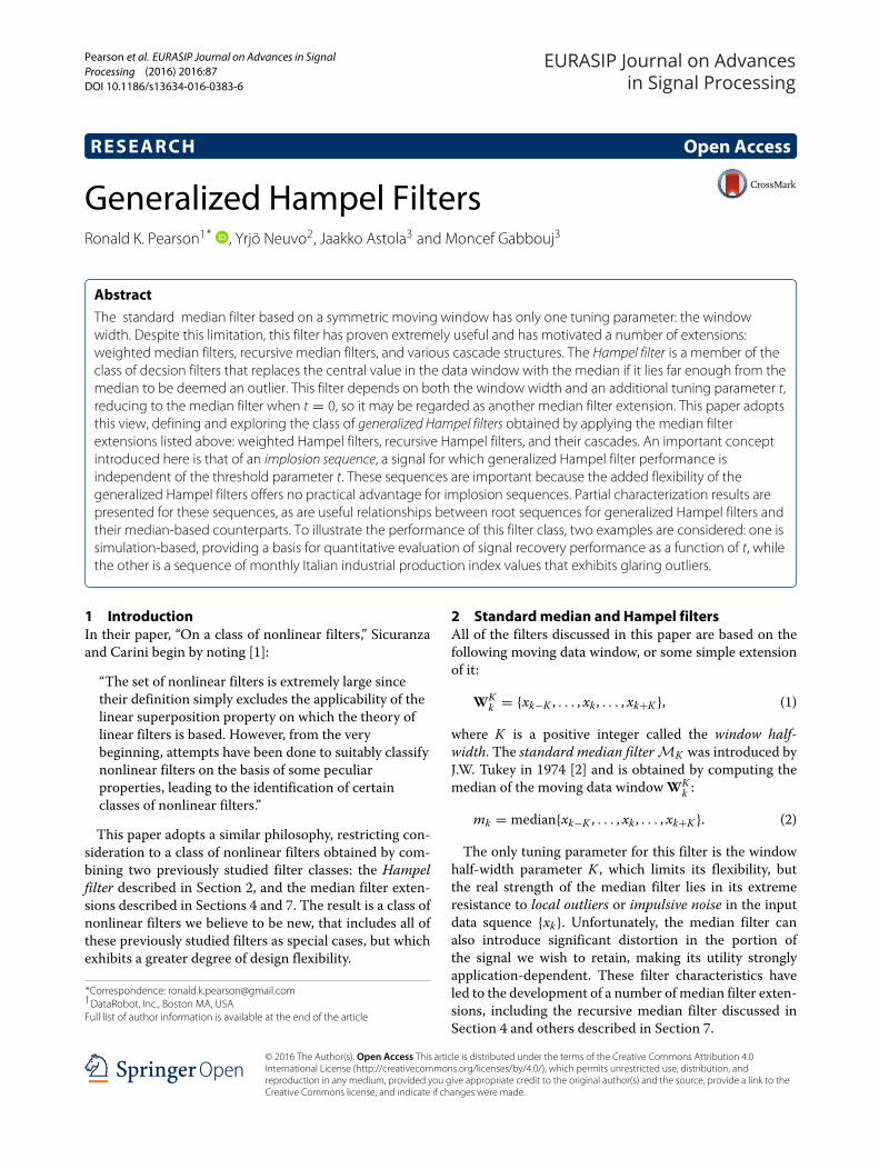
5 The influence of t on filter performanceTo provide quantitative filter performance results, the fol-lowing section presents a brief case study that examinesthe influence of the Hampel filter tuning parameter t onthe performance of both the standard Hampel filter andthe recursive Hampel filter. Since the primary questionof interest is the influence of the tuning parameter t, thisexample considers a fixed window half-width parameter(specifically, K = 5, yielding an 11-point moving win-dow filter) and examines filter performance over a rangeof t values. The basis for these performance comparisonsis a simulated data example described in Section 5.1: theadvantage of considering a simulation-based example isthat we can be explicit about the signal components wewish to recover and can therefore quantify signal recoveryperformance. More specifically, this example considerstwo possible signal recovery problems described in detailin Section 5.1 and characterizes performance in termsof two metrics: the root mean square signal recoveryerror (RMSE) and the mean absolute signal recovery error(MAE).

5.1 A simulated data exampleTo provide a basis for comparing the different filters con-sidered in this paper, we apply them to the 420-pointsimulated data sequence shown in Fig. 1, which containsfour components:

1. Step-and-ramp sequence (median filter root) fork = 1, 2, . . . , 420;

2. Low-level Gaussian noise (partial: nonzero only fork = 1, 2, . . . , 240);

3. Sinusoid (partial: nonzero only fork = 101, 102, . . . , 420);

4. Impulsive noise, randomly distributed throughoutthe sequence.

More specifically, the step-and-ramp sequence consistsof eight segments:

1. yk = 0 for k = 1 to k = 40;2. a linear increase from yk = 0 to yk = 1 from k = 41

to k = 100;3. yk = 1 for k = 101 to k = 140;4. yk = 2 for k = 141 to k = 220;5. a linear decrease from yk = 2 to yk = 0 from k = 221

to k = 300;6. yk = 0 for k = 301 to k = 320;7. yk = −1 for k = 321 to k = 400;8. yk = 0 for k = 401 to k = 420.

TheGaussian noise component hasmean zero and stan-dard deviation σ = 0.1, and the sinusoid has period 29 andamplitude 0.3. The impulsive noise component is an addi-tive term that is zero everywhere except for the followingeight values of k, where it takes the nonzero values indi-cated in parentheses: k = 20 (+1), k = 35 (−1), k = 120(+1), k = 190 (−1.5), k = 220 (−2.5), k = 300 (+1),k = 350 (+2.5), and k = 410 (+1.5).The primary question of interest here is how well the

different filters considered eliminate the isolated spikesin this signal while preserving the low-level details, espe-cially the sinusoidal component. The presence of thelow-level noise in approximately the first half of the sig-nal raises a subtle practical issue, however: is a “good”filter one that simply removes the impulsive spikes fromthe data sequence, or should it also address the low-levelnoise? Given that median filters and their extensions aremuch better suited to the removal of impulsive noise thanthe smoothing of low-level noise, the first formulationseems the more reasonable here, but the question is raisedto emphasize that filter performance criteria are generallyproblem-specific.Additional insights can be obained from this example

by considering filter performance for the three qualita-tively distinct signal subsequenes separated by dashedvertical lines in Fig. 1. Specifically, the first 100 points ofthe sequence—denoted “Noise Only” in Fig. 1—consistsof a median filter root sequence, contaminated with bothlow-level Gaussian noise and impulsive noise spikes. Thesecond subsequence, from k = 100 to k = 240 andlabelled “Noise + Sine,” contains all four of the signal com-ponents listed above, while the third subsequence, fromk = 240 to k = 420 and labelled “Sine Only,” consists of amedian filter root sequence with a superimposed sinusoidand isolated spikes, but no low-level noise.The two signal recovery problems considered here are

the following:

P1 the impulsive noise removal problem, where thesignal to be recovered consists of the sum of the firstthree components listed above;

Pearson et al. EURASIP Journal on Advances in Signal Processing (2016) 2016:87 Page 5 of 18

Fig. 1 A simulated 420-point signal

P2 the complete noise removal problem, where thesignal to be recovered consists of the sum of the twodeterministic components (i.e., the median filter rootplus the sinusoid), without either low-level orimpulsive noise.

As noted above, these signal recovery problems havedifferent characters, with the first being more suitablefor the filter class considered here, but the second prob-lem is of considerable practical significance. Two perfor-mance measures are considered for both problems: theroot-mean-square recovery error (RMSE) is more widelyused, but may be less appropriate than the mean absoluterecovery error (MAE) in the presence of impulsive noise.Finally, it is important to note that, for the filter window

width considered here (K = 5), the signal sequence shownin Fig. 1 is implosion-free and is not a median filter rootsequence. Thus, it follows that filter performance shoulddepend on the threshold parameter t, and the objective ofthe following discussions is to illuminate the nature of thisdependence.

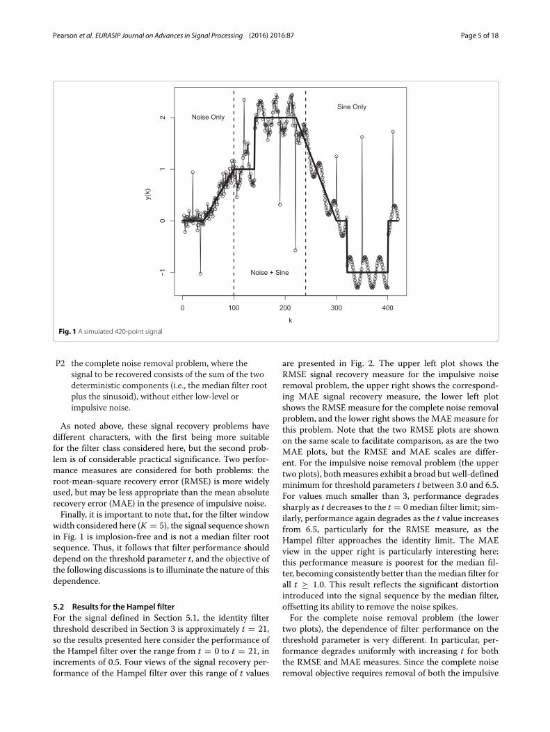
5.2 Results for the Hampel filterFor the signal defined in Section 5.1, the identity filterthreshold described in Section 3 is approximately t = 21,so the results presented here consider the performance ofthe Hampel filter over the range from t = 0 to t = 21, inincrements of 0.5. Four views of the signal recovery per-formance of the Hampel filter over this range of t values

are presented in Fig. 2. The upper left plot shows theRMSE signal recovery measure for the impulsive noiseremoval problem, the upper right shows the correspond-ing MAE signal recovery measure, the lower left plotshows the RMSE measure for the complete noise removalproblem, and the lower right shows the MAE measure forthis problem. Note that the two RMSE plots are shownon the same scale to facilitate comparison, as are the twoMAE plots, but the RMSE and MAE scales are differ-ent. For the impulsive noise removal problem (the uppertwo plots), bothmeasures exhibit a broad but well-definedminimum for threshold parameters t between 3.0 and 6.5.For values much smaller than 3, performance degradessharply as t decreases to the t = 0 median filter limit; sim-ilarly, performance again degrades as the t value increasesfrom 6.5, particularly for the RMSE measure, as theHampel filter approaches the identity limit. The MAEview in the upper right is particularly interesting here:this performance measure is poorest for the median fil-ter, becoming consistently better than themedian filter forall t ≥ 1.0. This result reflects the significant distortionintroduced into the signal sequence by the median filter,offsetting its ability to remove the noise spikes.For the complete noise removal problem (the lower

two plots), the dependence of filter performance on thethreshold parameter is very different. In particular, per-formance degrades uniformly with increasing t for boththe RMSE and MAE measures. Since the complete noiseremoval objective requires removal of both the impulsive

Pearson et al. EURASIP Journal on Advances in Signal Processing (2016) 2016:87 Page 6 of 18

Fig. 2 Hampel filter performance vs. t by four different criteria: RMSE or MAE, impulsive noise removal or complete noise removal

noise and the low-level noise, these results suggest that ast increases, the Hampel filter allows more of the low-levelnoise to pass through the filter unmodified, offsetting theperformance advantage of lower distortion of the sinu-soidal signal components. In particular, since the filterremoves all of the impulsive noise spikes for t between 0and 6.5, it follows that the poorer performance seen for thecomplete noise removal problem over the impulsive noiseremoval optimal performance range (t = 3.5 to t = 6.0)relative to the median filter limit t = 0 is caused by thefilter’s allowing more low-level noise into the output sig-nal. These results emphasize the point made earlier thatthese filters are not well-suited to low-level noise removalproblems.Figure 3 shows the MAE performance for the impul-

sive noise removal problem as a function of t, brokendown by signal segment: the upper left plot correspondsto the upper right plot in Fig. 2, characterizing the com-plete signal sequence, while the other three plots show thecorresponding results for the three segments indicated inFig. 1. The upper right plot presents the results for Seg-ment 1 (“Noise only”), consisting of the median filter rootsequence, low-level Gaussian noise, and impulsive noise

spikes. This plot clearly shows the low-level noise dis-tortion effects for small t values, which is worst for themedian filter (t = 0), decreasing monotonically until t =3.0, where the filter is sufficiently non-aggressive to allowmost of the low-level noise through unmodified. In fact,the optimal filter performance for this signal sequenceoccurs at t = 8.5 where the MAE is near zero. For t ≥ 9.5,the filter begins allowing impulsive noise spikes into theoutput, causing a dramatic increase in MAE. The lowerleft plot in Fig. 3 shows the results for Segment 2 (“Noise +Sine”). As in Segment 1, the performance is worst forthe median filter, improving uniformly with increasing tuntil the optimal plateau between t = 3.0 and t = 6.5,where the filter is aggressive enough to remove all of theimpulsive noise spikes but forgiving enough to pass thelow-level noise and sinusoidal components without dis-tortion. As t increases beyond this range, the Hampel filterquickly becomes an identity filter, passing all of the impul-sive noise spikes for t ≥ 9.5. Finally, for Segment 3 (“Sineonly,” lower right plot), the distortion introduced in thesinusoidal component by the median filter reduces essen-tially to zero for t ≥ 1.0 and the Hampel filter exhibitsoptimal performance for 1.0 ≤ t ≤ 6.5. As t increases

Pearson et al. EURASIP Journal on Advances in Signal Processing (2016) 2016:87 Page 7 of 18

Fig. 3 Hampel filter MAE performance vs. t for impulsive noise removal: full sequence (upper left), Segment 1 (upper right), Segment 2 (lower left), andSegment 3 (lower right)

beyond this limit, the filter begins to pass impulsive noisespikes, becoming an identity filter for t ≥ 14.0.Figure 4 shows a plot of the median filter response (t =

0, represented by open circles), overlaid with a solid linerepresenting the response of the Hampel filter with t = 5,falling in the optimal parameter range for the completesignal and all segments except Segment 1, where the per-formance is near-optimal. In addition, points where thesetwo filter responses differ are indicated by solid rectan-gles. From these results, it is clear that the Hampel filterwith t = 5 passes both the low-level noise componentsand the sinusolidal components essentially perfectly, whilethe median filter seriously distorts the portions of the sig-nal contaminated with low-level noise, and it “clips” thetops and bottoms of the sinusoidal component. It is alsoclear that both filters remove all of the impulsive noisefrom the signal sequence.The frequency of the sinusoidal component in this

example is important. Specifically, the maximum possi-ble frequency is that of the binary implosion sequencedescribed in Section 3, implying that in this limit, theHampel filter offers no advantage over the median filter.At the other extreme, if the sinusoidal frequency is low

enough, the N-point finite signal sequence will be mono-tonic, and thus a root sequence for the median filter andall Hampel filters. For intermediate frequencies; however,sinusoidal components are neither implosion sequencesnor roots, and as this example illustrates, the responseof the Hampel filter to these components generally variesstrongly with t.

5.3 Results for the recursive Hampel filterFigure 5 shows the complete sequence performance forthe recursive Hampel filter. Specifically, the upper leftplot shows the RMSE measure versus t for the impul-sive noise removal problem, while the upper right plotshows the correspondingMAE results; the lower two plotspresent these same results for the complete noise removalproblem. Comparing the upper two plots in Fig. 5 withthose in Fig. 2, we see the same general behavior of therecursive Hampel filter as that for the standard Hampelfilter, although the “optimal plateau” starts later and isslightly shorter. Indeed, Fig. 6 shows that the low-leveldistortion is worse for the recursive median filter thanthat for the standard median filter, although it declinesrapidly with increasing t until the optimal plateau is

Pearson et al. EURASIP Journal on Advances in Signal Processing (2016) 2016:87 Page 8 of 18

Fig. 4Median filter response (open circles) and Hampel filter response with t = 5 (lines), with points of disagreement marked as solid squares

Fig. 5 Recursive Hampel filter performance vs. t by four different criteria: RMSE or MAE, impulsive noise removal or complete noise removal

Pearson et al. EURASIP Journal on Advances in Signal Processing (2016) 2016:87 Page 9 of 18

Fig. 6 Recursive (solid triangles) and non-recursive (open circles) Hampel filter MAE performance vs. t for impulsive noise removal

reached, after which the two filter responses appear to beidentical.The more interesting results in Fig. 5 are the two bot-

tom plots for the complete noise removal problem: incontrast to the monotonic behavior seen in the corre-sponding plots in Fig. 2, the recursive filter exhibits asharp optimum at t = 1. A more detailed comparison ofthe recursive and nonrecursive Hampel filter MAE per-formance is shown in Fig. 7: for small t, the recursivefilter performance is much worse than the standard filter,although for t values between 1.0 and 3.0, the recursivefilter actually performs slightly better; for larger t values,both filters exhibit essentially identical performance.Figure 8 summarizes the recursive median filter’s MAE

performance for the complete noise removal problem asa function of t for the complete signal and the three seg-ments marked in Fig. 1. The upper left plot shows theresults for the complete signal and is the same as thelower right plot in Fig. 5, included here to facilitate visualcomparisons. The upper right plot shows the results forSegment 1 (“Noise only”) and here, the optimum at t = 1is much sharper than that for the complete signal, withperformance degrading much more rapidly as t increasesbeyond this value. The results for Segment 2 (“Noise +sine”) shown in the lower left plot are a bit more compli-cated: optimal performance is again obtained for t = 1,but this optimum is shallower than that for Segment 1 andthere is a second, small local minimum from t = 2.5 to t =3, after which performance again degrades monotonically

with increasing t. Finally, the performance for Segment 3(“Sine only”, lower right plot) is virtually identical to thatseen for the standard Hampel filter shown in the lowerright plot in Fig. 3.Overall, these results—particularly those for the com-

plete noise removal performance of the recursive Hampelfilter—show that the performance of these filters dependsstrongly on the threshold value t, but very differently fordifferent signal extraction problems and different signalcharacteristics. For example, for Segment 3 (“Sine only”),the performance of the recursive and standard Hampelfilters are almost identical, both for the impulse noiseremoval problem and for the complete noise removalproblem: distortion is observed for t less than 1.0, excel-lent performance is observed for t between 1.0 and 6.5,with consistent performance degradation as t is increasedbeyond this value. In contrast, for Segment 1 (“Noiseonly”), these performance curves are very different: forthe impulsive noise removal problem with the standardHampel filter, performance is worst in the median filterlimit, improves uniformly as t increases to 3.5 where itremains near-optimal as t increases to 8.5; optimalperformance—only slightly better—is achieved for tbetween 8.5 and 9.0, after which performance becomesdiscontinuously worse, but never approaches the level ofpoor performance seen for the median filter. In contrast,for the complete noise removal problemwith the recursiveHampel filter for this data segment, a sharp optimum isobserved at t = 1.0, with increasingly poorer performance

Pearson et al. EURASIP Journal on Advances in Signal Processing (2016) 2016:87 Page 10 of 18

Fig. 7 Recursive (solid triangles) and non-recursive (open circles) Hampel filter MAE performance vs. t for complete noise removal

as t increases, exhibiting worse performance than therecursive median filter for all t > 2. Finally, as noted,the complete noise removal performance for the recur-sive Hampel filter for Segment 2 (“Noise + sine”) is evenmore complicated, exhibiting local optima in its MAE vs.t performance curve.

6 A real data exampleTo provide an illustration of how the generalized Hampelfilters described in this paper work with a real data exam-ple, the following section applies several of these filtersto a publically-available time-series dataset. Specifically,this example is based on the gipi sequence included inthe tsoutliers R package [8], available as one row of thebde9915 data frame. This data sequence is a monthlytime-series of Italian industrial production index from1981 to 1996, consisting of 192 observations. A plot ofthis time-series is shown in Fig. 9, from which the pres-ence of significant outliers in the data is clear. In fact,these anomalous data points occur at regular 12-monthintervals and represent what Kaiser and Maravall call sea-sonal outliers [9]. If we apply standard time-series mod-eling procedures (e.g., fitting ARMA or ARIMA modelsto the data), the results will be profoundly influenced bythe presence of these outliers, and at least two generalstrategies can be used to address these problems. Thefirst is the development of specialized analysis procedures

that are resistant to the anomalies in the data, extendingstandard analysis methods using fundamental ideas fromrobust statistics, such as the robust time-series model-ing approach described by Martin and Yohai [10] or therobust-resistant spectrum estimation approach describedby Martin and Thomson [11]. The second approach is theuse of simple data-cleaning filters like those described inthis paper to remove the outliers from the data sequence,after which standard analysis procedures are applied. Theprimary objective of this example is to illustrate the rangeof results that may be obtained when different general-ized Hampel filters are applied to the time-series shown inFig. 9.Figure 10 shows the results of two standard median fil-

ters (upper two plots) and two recursive median filters(lower two plots) applied to the Italian industrial produc-tion data shown in Fig. 9. The left-hand plots correspondto filters based on the window half-width parameter K =3 (i.e., 7-point moving data windows), while the right-hand plots correspond to filters with K = 5 (i.e., 11-pointmoving data windows). In all cases, the vertical scale isthe same to facilitate comparisons. All of these filterscompletely eliminate the seasonal outliers, but they alsointroduce significant distortion in the nominal part of thesignal. This is less pronounced in the standard medianfilter results, where the original signal details are muchbetter approximated than in the results obtained from the

Pearson et al. EURASIP Journal on Advances in Signal Processing (2016) 2016:87 Page 11 of 18

Fig. 8 Recursive Hampel filter MAE performance vs. t for complete noise removal: full sequence (upper left), Segment 1 (upper right), Segment 2(lower left), and Segment 3 (lower right)

recursive median filters. It is also clear that the distortionintroduced by these filters is worse for K = 5 than it is forK = 3.Figure 11 shows comparative results for four different

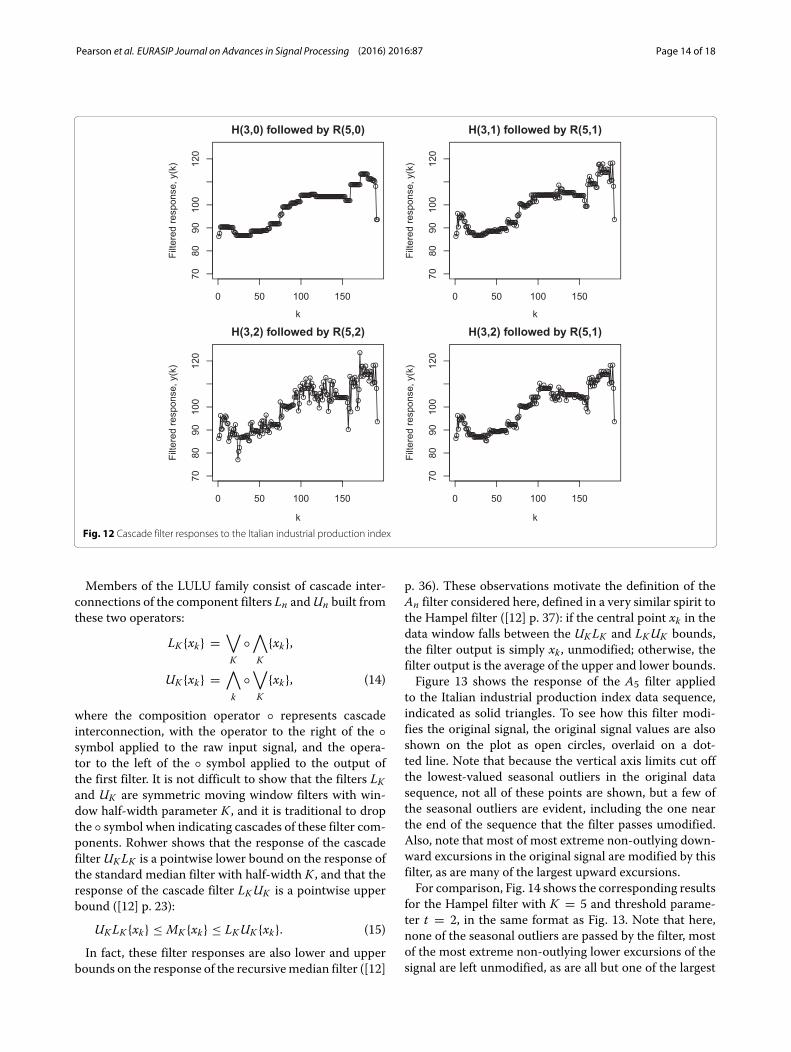
Hampel-based filters. As in Fig. 10, the top two plots arefor nonrecursive Hampel filters, while the bottom twoplots are for their recursive counterparts. Here, all of thesefilters are based on the half-width parameter K = 5,with the right- and left-hand plots differing in the Ham-pel threshold parameter t. Specifically, the left-hand plotscorrespond to the more aggressive threshold value t = 1,while the right-hand plots are based on t = 2. As before,all of these filters completely eliminate the seasonal out-liers from the data, introducingmuch less distortion in thenominal part of the signal than the corresponding medianfilters do. Comparing the left-hand and right-hand plots,it is also clear that these filters introduce much less distor-tion with t = 2 than with t = 1. Comparing the upper andlower plots, it is also clear that while the recursive Ham-pel filter introduces more nominal signal distortion thanthe nonrecursive filter for this signal, this effect becomesmuch less pronounced with increasing t.

One type of generalized Hampel filter that was not dis-cussed in connection with the simulation example wasthe subclass of cascade interconnections of Hampel fil-ters and/or recursive Hampel filters. Figure 12 shows theresults obtained when four different filter cascades areapplied to the Italian industrial production index datashown in Fig. 9. In the upper left plot, the results wereobtained by first applying the standard median filter withK = 3 (i.e., the 7-point median filter) to the raw signal,and then applying the recursive median filter with K = 5(i.e., the 11-point recursive median filter) to the outputof this filter. Comparing this plot with those for eitherof the individual components of this cascade in Fig. 10(i.e., the standard median filter with K = 3 shown in theupper left plot and the recursive median filter with K = 5shown in the lower right plot), it is clear that the cascaderesults are intermediate in their tendency to emphasizethe low-frequency trend in the data at the expense ofkey high-frequency details, while still removing the sea-sonal outliers. The upper right plot in Fig. 12 relaxes bothcomponents of this first cascade, increasing the thresh-old parameter from the median filter limit t = 0 to the

Pearson et al. EURASIP Journal on Advances in Signal Processing (2016) 2016:87 Page 12 of 18

Fig. 9Monthly Italian industrial production index, 1981–1996

Fig. 10Median filter and recursive median responses to the Italian industrial production index

Pearson et al. EURASIP Journal on Advances in Signal Processing (2016) 2016:87 Page 13 of 18

Fig. 11 Hampel filter and recursive Hampel filter responses to the Italian industrial production index

less aggressive value t = 1. Here, intermediate and high-frequency details are better preserved than in the medianfilter cascade results shown to the left, giving a result withfewer “flat streches” than seen for the recursive Hampelfilter with t = 1 shown in the lower left plot in Fig. 11. Thelower left plot in Fig. 12 represents the next step in thisgeneral trend, keeping the same basic cascade structure asin the previous two examples, but further increasing thethreshold parameter for both filter components to t = 2.Interestingly, this cascade filter response preserves muchless of the original nominal signal detail than the recursiveHampel filter with K = 5, as may be seen by compar-ing this result with the lower right plot in Fig. 11. Finally,the lower right plot in Fig. 12 shows the results of a sim-ilar cascade, but with the threshold of the recursive filterreduced from t = 2 as in the lower left plot to t = 1.As expected, by making this second cascade componentmore aggressive, we further attenuate many of the originalsignal details relative to the response shown in the lowerleft plot, but not nearly as much as in the still more aggres-sive cascade shown in the upper right plot directly above.The key point of this example is to demonstrate that cas-cade interconnection of simpler generalized Hampel filtercomponents can significantly expand the range of possiblefilter behavior.

The final result presented here considers a filter that isnot a member of the generalized Hampel family, but isconceptually similar in an important sense. Specificallly,recall that the basic idea behind the Hampel filter is toconsider the central point in the moving data window anddetermine whether it is “anomalous:” if so, it is replacedwith the “more reasonable” median value computed fromthe data window; otherwise, it is left unmodified. The Anfilter described by Rohwer ([12] p. 37) is based on a simi-lar idea, but with a different definition of “anomalous” anda different replacement value for these points. This filterbelongs to the LULU family, described briefly here; for amore detailed introduction, refer to Rohwer’s book [12].A less detailed introduction to these filters is also givenin the book by Pearson and Gabbouj ([13] Section 6.2.3),which also provides Python implementations in the Non-linearDigitalFiltersmodule.The LULU filter class consists of filters constructed

from cascade interconnections of the following two asym-metric moving window operators:

∨K

{xk} = max{xk , xk+1, . . . , xk+K }∧K

{xk} = min{xk−K , . . . , xk−1, xk}. (13)

Pearson et al. EURASIP Journal on Advances in Signal Processing (2016) 2016:87 Page 14 of 18

Fig. 12 Cascade filter responses to the Italian industrial production index

Members of the LULU family consist of cascade inter-connections of the component filters Ln andUn built fromthese two operators:

LK {xk} =∨K

◦∧K

{xk},

UK {xk} =∧k

◦∨K

{xk}, (14)

where the composition operator ◦ represents cascadeinterconnection, with the operator to the right of the ◦symbol applied to the raw input signal, and the opera-tor to the left of the ◦ symbol applied to the output ofthe first filter. It is not difficult to show that the filters LKand UK are symmetric moving window filters with win-dow half-width parameter K , and it is traditional to dropthe ◦ symbol when indicating cascades of these filter com-ponents. Rohwer shows that the response of the cascadefilter UKLK is a pointwise lower bound on the response ofthe standard median filter with half-width K , and that theresponse of the cascade filter LKUK is a pointwise upperbound ([12] p. 23):

UKLK {xk} ≤ MK {xk} ≤ LKUK {xk}. (15)

In fact, these filter responses are also lower and upperbounds on the response of the recursivemedian filter ([12]

p. 36). These observations motivate the definition of theAn filter considered here, defined in a very similar spirit tothe Hampel filter ([12] p. 37): if the central point xk in thedata window falls between the UKLK and LKUK bounds,the filter output is simply xk , unmodified; otherwise, thefilter output is the average of the upper and lower bounds.Figure 13 shows the response of the A5 filter applied

to the Italian industrial production index data sequence,indicated as solid triangles. To see how this filter modi-fies the original signal, the original signal values are alsoshown on the plot as open circles, overlaid on a dot-ted line. Note that because the vertical axis limits cut offthe lowest-valued seasonal outliers in the original datasequence, not all of these points are shown, but a few ofthe seasonal outliers are evident, including the one nearthe end of the sequence that the filter passes umodified.Also, note that most of most extreme non-outlying down-ward excursions in the original signal are modified by thisfilter, as are many of the largest upward excursions.For comparison, Fig. 14 shows the corresponding results

for the Hampel filter with K = 5 and threshold parame-ter t = 2, in the same format as Fig. 13. Note that here,none of the seasonal outliers are passed by the filter, mostof the most extreme non-outlying lower excursions of thesignal are left unmodified, as are all but one of the largest

Pearson et al. EURASIP Journal on Advances in Signal Processing (2016) 2016:87 Page 15 of 18

Fig. 13 A5 filter applied to the monthly Italian industrial production index (solid triangles), overlaid on the original signal (dotted lines with open circles)

Fig. 14 Hampel filter (K = 5, t = 2) applied to the monthly Italian industrial production index (solid triangles), overlaid on the original signal (dottedlines with open circles)

Pearson et al. EURASIP Journal on Advances in Signal Processing (2016) 2016:87 Page 16 of 18

upper excursions. In fact, careful comparisons of all ofthe filter results presented here show that, if our filteringobjective is to remove only the seasonal outliers and leavethe rest of the signal unmodified, the Hampel filter withK = 5 and t = 2 gives the best performance of any of thefilters considered here. It is important to emphasize, how-ever, that analogous results cannot be expected to hold inall situations. For example, in cases where some degree ofsmoothing of the low-level noise is also desirable, cascadefilters like that shown in the lower right plot in Fig. 12may bemuch better choices. The key point of this examplehas been to illustrate, first, the range of behavior pos-sible when applying various members of the generalizedHampel filter class to a real data sequence, and second,to provide a comparison with a useful data cleaning filterthat does not belong to this class.

7 Other generalizations of the Hampel filter7.1 Weighted filtersWeighted median filters are obtained by replacing themoving window WK

k defined in Eq. (1) with the followingweighted data window:

Qk = {w−K � xk−K , . . . ,w0 � xk , . . . ,wK � xk+K }, (16)

where the operator � denotes replication (m � xj cre-ates a set with the data value xj replicated m times),and {w−K , . . . ,w0, . . . ,wK } represents a sequence of pos-itive integer weights. This extension greatly increases themedian filter’s flexibility, but it also greatly complicatesthe analysis of filter characteristics; for example, no com-plete characterization of the root sequences of arbitrarilyweighted median filters is known. For a more detailed dis-cussion of this filter class and what is known about it, referto the survey paper by Yin et al. [14].The weighted Hampel filter is defined by replacing the

original data windowWKk in the definition of the standard

Hampel filter with the weighted window Qk defined inEq. (16). Specifically, the weighted Hampel filter is definedby:

yk ={xk |xk − mk(Q)| ≤ tSk(Q),mk |xk − mk(Q)| > tSk(Q), (17)

where mk(Q) is the median of the weighted window Qkand Sk(Q) is the corresponding MAD scale estimator. Aswith the standard Hampel filter, note that the weightedHampel filter reduces to the weighted median filter fort = 0, and the root sequence nesting condition for thesefilters—for fixed weights—follows as before: s ≤ t impliesRs ⊂ Rt . Similarly, the concept of implosion sequencesintroduced in Section 3 also applies to the weightedHampel filters, but the conditions for {xk} to be an implo-sion sequence now depend on the filter weights {wk}.Given the lack of a general characterization for weightedmedian filter root sequences noted above and the strong

connection between standard Hampel filter implosionsequences and standard median filter roots shown inSection 3, it is likely that a complete characterizationof weighted Hampel filter implosion sequences will bechallenging.

7.2 Weighted recursive filtersThe class of weighted recursive median filters is obtainedby adopting both of the modifications just described:using the recursive moving window RK

k defined inSection 4 with the weight-based replication schemedescribed in Section 7.1. Specifically, the resulting movingdata window has the form:

Zk = {w−K � yk−K , . . . ,w0 � xk , . . . ,wK � xk+K }, (18)

where yk−j is the output of the weighted median filter atprior sample k − j. Since this median filter generalizationincludes both of the previous ones as proper subsets, theflexibility of this class is even greater, as is the complexityof its analysis. The survey paper by Yin et al. also includesa discussion of these filters [14].The weighted recursive Hampel filter is defined by

replacing the original data window Rt,Kk in the definition

of the recursive Hampel filter with the weighted windowZk defined in Eq. (18) where yk−j is the output of theweighted Hampel filter defined in Section 7.1 at time k− j.Specifically, the weighted Hampel filter is defined by:

yk ={xk |xk − mk(Z)| ≤ tSk(Z),mk |xk − mk(Z)| > tSk(Z), (19)

wheremk(Z) is the median of the recursive weighted win-dow Zk and Sk(Z) is the corresponding MAD scale esti-mator. It follows by the reasoning presented in Section 4that the recursive weighted Hampel filter root sets areidentical with the non-recursive weighted Hampel filterroot sets, and that the recursive weighted Hampel fil-ter root sets nest for increasing threshold parameterst. Again, it is likely that complete characterizations ofthe weighted recursive Hampel filter root sequences andimplosion sequences will be challenging.

7.3 Extensions to image processingA detailed discussion of the extension of the one-dimensional generalized Hampel filters discussed here toimage processing applications is beyond the scope of thispaper, but this extension is important enough to warranta brief discussion. All of the filters defined in this papercan be extended to two-dimensional images in at leasttwo different ways. The first and simpler is analogousto that described in Section 1.3.3 of the book by Astolaand Kuosmanen [3]: the one-dimensional moving window

Pearson et al. EURASIP Journal on Advances in Signal Processing (2016) 2016:87 Page 17 of 18

considered here can be replaced by a square (2K + 1)×(2K + 1) two-dimensional window that is moved acrossthe image. The median and MAD scale estimate can thenbe computed from these (2K+1)2 pixel intensities exactlyas in the one-dimensional case, and the same logic appliedas before: if the central point in the data window lies morethan t times the MAD scale estimate from the medianvalue, the filter’s output is themedian value; otherwise, thefilter’s output is the unmodified central value. As in theone-dimensional case, setting t = 0 reduces this filter tothe two-dimensional median filter, and increasing tmakesthe filter less aggressive.Two-dimensional recursive filters are also possible, gen-

eralizing the two-dimensional recursive median filter,although as noted by Astola and Kuosmanen, the resultsobtained with this filter will depend on the order in whichthe pixels are processed ([3] p. 203). That is, since thereis no unique total order on the points in an image, it isnecessary to impose such an order for the “prior filter out-puts” required in a recursive filter implementation to bewell-defined. This can be done in different ways (e.g., left-to-right lexical order, top-to-bottom lexical order, etc.),generally yielding different results.Finally, an alternative approach is to construct multi-

stage Hampel image processing filters that combine theoutputs of subfilters like those discussed by Nieminen andNeuvo [15], corresponding to vertical, horizontal, diago-nal, cross- or x-shaped subwindows applied to the image.This general construction is described in Section 3.7 ofthe book by Astola and Kuosmanen [3], and it can also bereadily extended to generalized Hampel filters by simplyreplacing the median filters defined on these subwindowswith the corresponding Hampel filters.

8 ConclusionsThe Hampel filter introduced in Section 2 is effectivelya moving window outlier detector that replaces the orig-inal signal value with the median filter response if thatvalue is deemed an outlier. This determination is basedon a threshold parameter t chosen by the user and theMAD scale estimate for the moving window, and the fil-ter reduces to the standard median filter if t = 0. Thecentral idea of this paper was to view the Hampel fil-ter as a generalization of the median filter and ask whatthe consequences of this generalization are, first for thestandard Hampel filter and then for novel extensions likethe recursive Hampel filter. One important aspect of thisinvestigation was the partial characterization in Section 3of implosion sequences, for which this generalization hasno effect: these are sequences for which the responseof the Hampel filter is independent of t. In addition, itwas shown that Hampel filter root sequences nest, withthe median filter root set included in all Hampel filterroot sets. Thus, the input sequences of greatest interest

here are neither implosion sequences nor root sequences,where the Hampel filter may be tuned from its mostaggressive limit (t = 0, corresponding to themedian filter)to an identity filter for sufficiently large t.A detailed description of the recursive Hampel filter was

given in Section 4, where it was shown that this filter’s rootset for each t is the same as the standardHampel filter rootset for the same value of t, generalizing the well-knownresult for the recursive median filter [7]. One of the inter-esting characteristics of the recursive median filter is itsidempotence—the fact that it reduces any input sequenceto a root sequence in a single pass—and an intriguingquestion is whether this behavior extends to the recursiveHampel filter for any t > 0.Section 5 presented a brief simulation-based case study

exploring the performance of the standard and recur-sive Hampel filters as a function of t for a simulatedsignal sequence that was neither a median filter rootsequence nor an implosion sequence. More specifically,this signal consisted of a median filter root sequence withthree additional components superimposed on it: low-level Gaussian noise for one part of the signal, a sinusoidfor another part of the signal, and impulsive noise spikes.Two performance measures were considered—RMSE andMAE—for two signal recovery problems: impulsive noiseremoval, and a complete noise removal problem that alsoattempted to remove low-level Gaussian noise from thesignal. Not surprisingly, performance was much betterfor the impulsive noise removal problem, but the realpoint of this example was to provide specific illustrationsof how much performance does depend on t, and howstrongly this dependence varies between different prob-lem formulations and signal characteristics (e.g., differentsignal subsequences exhibiting different combinations ofthe components listed above).To provide a more representative illustration of the per-

formance of generalized Hampel filters, Section 6 appliedseveral members of this filter class to a monthly Italianindustrial production index series that contains glaringoutliers every 12 months (seasonal outliers [9]). The fil-ters applied to this example included the standard andrecursive median filters for two different window half-width parameters, both standard and recursive Hampelfilters, and four cascade interconnections of filters fromthe generalized Hampel family. If our objective is sim-ply the removal of the seasonal outliers, it appears thatthe standard Hampel filter with a sufficiently large thresh-old parameter t is the optimum choice here, but one ofthe points illustrated by these filtering results was thatcascade interconnections of Hampel and recursive Ham-pel filters exhibit smoothing behavior that is much lessextreme than that of the recursive median filter and whichmay be advantageous in some applications. For compar-ison, results were also presented for a promising data

Pearson et al. EURASIP Journal on Advances in Signal Processing (2016) 2016:87 Page 18 of 18

cleaning filter that is not a member of the generalizedHampel family: theAn filter defined by Rohwer ([12] p. 37)from the LULU filter family. For this example, the An fil-ter was not sufficiently aggressive, failing to eliminate theleast extreme of the seasonal outliers in the data sequence,but again, it is important to emphasize that the “best” fil-ter can be expected to depend strongly on the details ofthe application.Finally, three other generalizations of the Hampel filter

were described briefly in Section 7: the weighted Hampelfilter, the recursive weighted Hampel filter, and exten-sions to two-dimensional image processing applications.The first two of these filters are generalizations of theweighted median filter and the recursive weighted medianfilter, respectively, which are more difficult to character-ize than their non-weighted counterparts. For this reason,characterizations of roots, implosion sequences, and otherperformance characteristics of these generalized Hampelfilters appears likely to be much more challenging thanthe corresponding characterizations of the standard andHampel recursive filters. Finally, while a detailed treat-ment of image processing applications is beyond the scopeof this paper, the one-dimensional filters described herecan all be extended to these applications in much the sameway as median filters have been.

Competing interestsThe authors declare they have no competing interests.

Received: 20 April 2016 Accepted: 25 July 2016

References1. GL Sicuranza, A Carini, in Festschrift in Honor of Jaakko Astola on the

Occasion of his 60th Birthday, ed. by I Tabus, K Egiazarian, and M Gabbouj.On a class of nonlinear filters (Tampere International Center for SignalProcessing, Tampere, Finland, 2009), pp. 115–143

2. JW Tukey, Nonlinear (nonsuperposable) methods for smoothing data.Abstracts, Cong. Rec. EASCON-74, 673 (1974)

3. J Astola, P Kuosmanen, Fundamentals of nonlinear digital filtering. (CRCPress, Boca Raton, FL, USA, 1997)

4. L Davies, U Gather, The identification of multiple outliers. J. Am. Stat.Assoc. 88, 782–801 (1993)

5. J Astola, P Heinonen, Y Nuevo, On root structures of median andmedian-type filters. IEEE Trans. Acoustics Speech Signal Proc. 35,1199–1201 (1987)

6. NC Gallagher, GL Wise, A theoretical analysis of the properties of medianfilters. IEEE Trans. Acoustics, Speech, Signal Proc. 29, 1136–1141 (1981)

7. TA Nodes, NC Gallagher, Median filters: some modifications and theirproperties. IEEE Trans. Acoust. Speech Signal Proc. 30, 739–746 (1982)

8. López-de-Lacalle J, tsoutliers: Detection of Outliers in Time Series. Rpackage version 0.6 (2015). https://CRAN.R-project.org/package=tsoutliers

9. R Kaiser, A Maravall, Seasonal outliers in time series, Banco de Espana,Servicio de Estudios. Working paper number, 9915 (1999). http://www.bde.es/f/webbde/SES/Secciones/Publicaciones/PublicacionesSeriadas/DocumentosTrabajo/99/Fic/dt9915e.pdf

10. RD Martin, VJ Yohai, Influence Functionals for time series. Ann. Stat. 14,781–818 (1986)

11. RD Martin, DJ Thomson, Robust-resistant spectrum estimation. Proc. IEEE.70, 1097–1114 (1982)

12. Rohwer C, Nonlinear smoothing andmultiresolution Analysis. (Birkhäuser),(Basel, CH, 2005)

13. RK Pearson, M Gabbouj, Nonlinear digital filtering with Python. (CRC Press,Boca Raton, FL, USA, 2016)

14. L Yin, R Yang, M Gabbouj, Y Neuvo, Weighted median filters: a tutorial.IEEE Trans. Circ. Syst. II: Analog Digital Signal Process. 43, 157–192 (1996)

15. A Nieminen, Y Neuvo, Comments of theoretical anaysis of themax/median filter. IEEE Trans. Acoust. Speech Signal Proc. 36, 826–827(1988)

Submit your manuscript to a journal and benefi t from:

7 Convenient online submission

7 Rigorous peer review

7 Immediate publication on acceptance

7 Open access: articles freely available online

7 High visibility within the fi eld

7 Retaining the copyright to your article

Submit your next manuscript at 7 springeropen.com