Taming the Factor Zoo∗

Guanhao Feng†

College of Business

City University of Hong Kong

Stefano Giglio‡

Yale School of Management

NBER and CEPR

Dacheng Xiu§

Booth School of Business

University of Chicago

This Version: August 31, 2017

Abstract

The asset pricing literature has produced hundreds of potential risk factors. Organizing this

“zoo of factors” and distinguishing between useful, useless, and redundant factors require econo-

metric techniques that can deal with the curse of dimensionality. We propose a model-selection

method to systematically evaluate the contribution to asset pricing of any new factor, above and

beyond what a high-dimensional set of existing factors explains. Our methodology explicitly ac-

counts for potential model-selection mistakes, unlike the standard approaches that assume perfect

variable selection, which rarely occurs in finite sample and produces a bias due to the omitted

variables. We apply our procedure to a set of factors recently discovered in the literature. We

show that several factors – such as profitability and investments – have statistically significant

explanatory power beyond the hundreds of factors proposed in the past. In addition, we show that

our risk price estimates and their significance are stable, whereas the model selected by simple

LASSO is not.

Key words: Factors, Risk Price, Post-Selection Inference, Regularized Two-Pass Estimation,

Variable Selection, Machine Learning, LASSO, Elastic Net.

∗We appreciate insightful comments from Alex Belloni, John Campbell, John Cochrane, Chris Hansen, Lars Hansen,

Stefan Nagel and Chen Xue. We are also grateful for helpful comments from seminar and conference participants at

the City University of Hong Kong, Peking University, Renmin University, University of British Columbia, Luxembourg

School of Finance, the 2016 Financial Engineering and Risk Management Symposium in Guangzhou, 2017 EcoStat

Conference at Hong Kong University of Science and Technology, and University of Oregon Summer Finance Conference.

We acknowledge research support by the Fama-Miller Center for Research in Finance at Chicago Booth.†Address: 83 Tat Chee Avenue, Kowloon Tong, Hong Kong. E-mail address: gavin.feng@cityu.edu.hk.‡Address: 165 Whitney Avenue, New Haven, CT 06520, USA. E-mail address: stefano.giglio@yale.edu.§Address: 5807 S Woodlawn Avenue, Chicago, IL 60637, USA. E-mail address: dacheng.xiu@chicagobooth.edu.

1

1 Introduction

The search for factors that explain the cross section of expected stock returns has produced hundreds

of potential factor candidates, as noted by Cochrane (2011) and most recently by Harvey et al. (2015),

McLean and Pontiff (2016), and Hou et al. (2016). A fundamental task facing the asset pricing field

today is to bring more discipline to this “zoo” of factors. In particular, how can we discriminate

truly useful pricing factors from redundant and useless factors that appear significant due to data

mining? How do we judge whether a new factor adds explanatory power for asset pricing, relative

to the existing set of hundreds of factors the literature has so far produced?

This paper provides a framework for systematically evaluating the contribution of individual

factors relative to the myriad of existing factors the literature has proposed, and conducting appropri-

ate statistical inference in this high-dimensional setting. In particular, we show how to estimate and

test the marginal importance of any factor gt in pricing the cross section of expected returns beyond

what is explained by a high-dimensional set of potential factors ht, where gt and ht could be tradable

or non-tradable factors. We assume the true asset pricing model is approximately low-dimensional;

however, in addition to relevant asset pricing factors, gt and ht include redundant ones that add no

explanatory power to the other factors, as well as useless ones that have no explanatory power at

all. Selecting the relevant factors from ht and conducting proper inference on the contribution of gt

above and beyond those factors is the aim of this paper.

When ht consists of a small number of factors, testing whether gt is useful in explaining asset

prices while controlling for the factors in ht is straightforward: it simply requires estimating the

loadings of the stochastic discount factor on gt and ht (i.e., the price of risk of these factors), and

testing whether the price of risk of gt is different from zero (see Cochrane (2009)). This exercise not

only tells us whether gt is useful for pricing the cross section, but it also reveals how shocks to gt

affect marginal utility, which has a direct economic interpretation.

When ht consists of potentially hundreds of factors, however, standard statistical methods to

estimate and test risk prices become infeasible or result in poor estimates and invalid inference, be-

cause of the curse of dimensionality. Although dimension-reduction techniques (e.g., least absolute

shinkage and selection operator, LASSO) can be useful in (asymptotically) selecting the right model

and reducing the dimensionality of ht, they produce erroneous inference unless appropriate econo-

metric methods are used to explicitly account for the model-selection mistakes that can occur in any

finite sample (see Chernozhukov et al. (2015)). For example, simply applying a model-selection tool

like LASSO to a large set of factors and checking whether a particular factor gt is significant in that

sample (or even just checking if it gets selected) is not a reliable way to determine whether gt is

actually one of the true factors.

2

The methodology we propose in this paper marries these new econometric methods (in partic-

ular, the double-selection LASSO method of Belloni et al. (2014b)) with two-pass regressions such

as Fama-MacBeth to specifically estimate risk prices in a high-dimensional setting and evaluate the

contribution of a factor to explaining asset prices. Without relying on prior knowledge about which

factors to include as controls among the hundreds in ht, our procedure selects factors that are either

useful in explaining the cross section of expected returns or are useful in mitigating the omitted

variable bias problem due to potential model selection mistakes. We show that including both types

of factors as controls is essential to conduct correct inference on the price of risk of gt.

We apply our methodology to a large set of factors proposed in the last 30 years. We collect and

construct a factor data library, containing 99 risk factors. Additionally, we create nontradable and

nonlinear quadratic factors, including the squares of each of these 99 factors and their interactions

with the size factor, respectively. We perform a variety of empirical exercises that illustrate the

importance of accounting for model-selection mistakes when conducting inference about risk prices

and assessing the significance of new factors. We start by evaluating the marginal contribution of

recent factors proposed in the last five years to the large set of factors proposed before 2011. The

new factors include – among others – the two new factors introduced by Fama and French (2015)

and Hou et al. (2014), and the intermediary-based factors from He et al. (2016). Given that the set

of potential control factors includes nearly 250 factors, one might wonder whether, in practice, any

additional factor could make a significant contribution to explaining the cross section of expected

returns. We show that indeed several of these new factors (e.g., profitability and investment) have

significant marginal explanatory power for expected returns.

Second, we show that the results of this empirical exercise are stable across both the cross

section of test assets and time periods. We randomly select 2,000 subsamples with replacement from

our full sample, resampling in both the cross-sectional and time-series dimensions, and show that

our estimates of risk prices and their significance are stable across subsamples. In contrast, the

factors selected by simple LASSO in each subsample are not stable across subsamples. This result

underscores the fact that in finite samples LASSO will generally pick some wrong factors; therefore,

simple LASSO should not be used to determine whether any particular factor gt belongs to the true

model. Our double-selection procedure corrects for the potential mistakes by the LASSO selection

thanks to a second selection step, described in greater detail below, and produces valid inference

about the factors of interest despite the mistakes that occur at the factor-selection stage.

Third, we propose a recursive exercise in which factors are tested as they are introduced against

previously proposed factors. The exercise shows that our procedure would have deemed factors as

redundant or spurious in most cases, while finding significance for 14 of the factors (out of 99). Over

time, therefore, our procedure would have screened out many factors at the time of their introduction.

3

The double-selection (DS) estimation procedure we propose, that combines cross-sectional asset

pricing regressions with the double-selection LASSO of Belloni et al. (2014b) (designed originally for

linear treatment effect models), starts by using a two-step selection method to select “control” factors

from ht, and then estimates the risk price of gt from cross-sectional regressions that include gt and

the selected factors from ht.

As the name implies, the “double selection” of factors from ht happens in two stages; both

stages are crucial to obtain correct inference on gt. A first set of factors is selected from ht based

on their pricing ability for the cross-section of returns. Factors that appear to contribute little to

pricing assets are excluded from the set of controls. This first step – effectively an application of

standard LASSO to the set of potential factors ht – has the advantage of selecting factors based on

their usefulness in pricing the cross section of assets, as opposed to other commonly used selection

methods (e.g., principal components) that select factors based on their ability to explain the time-

series variation of returns. Using a cross-sectional approach is expected to deliver more relevant

factors for asset pricing.

This first step is, however, not sufficient to ensure valid inference on gt, because the LASSO

selection may exclude some factors that have small risk prices in sample, but whose covariance

with returns are nonetheless highly cross-sectionally correlated with exposures to gt. That is, in

any finite sample, we can never be sure that LASSO has selected the correct control model. Any

omission of relevant factors due to finite-sample model-selection errors distorts the inference on the

risk price of gt, leading to incorrect inference on the significance – and even the sign – of gt’s risk

price. This issue is a well-known problem with model-selection methods (see, for example, Leeb and

Potscher (2005)), and it has spurred a large econometrics literature on uniformly valid inference,

with important consequences for asset pricing tests that we explore in this paper.

To obtain correct asymptotic inference for gt, instead, including a second stage of factor se-

lection is crucial. The second step adds to the set of controls additional factors whose covariances

with returns are highly correlated in the cross section with the covariance between returns and gt.

Intuitively, we want to make sure to include even factors with small in-sample risk prices, if omitting

them may still induce a large omitted variable bias due to the cross-sectional correlation between

their risk exposures and the risk exposures to gt. It is also possible that some variables selected

from the second stage are useless or redundant, but their inclusion only leads to a moderate loss in

efficiency.

After selecting the set of controls from ht (including all factors selected in either of the two

selection stages), we conduct inference on gt by estimating the coefficient of a standard two-pass

regression using gt and the selected small number of control factors from ht. This post-selection

estimation step is also useful to remove biases arising from regularization in any LASSO procedure;

4

see, for example, Friedman et al. (2009). We then conduct asymptotic inference on the risk price

of gt using a central-limit result we derive in this paper. We show by simulation that our estimator

performs well in finite samples, and substantially outperforms alternative estimators.

Finally, it is worth pointing out an alternative motivation for the methodology proposed in

this paper. Theoretical asset pricing models often predict that some factors (gt) should be part

of the stochastic discount factor, i.e. they should enter the investors’ marginal utility. Theoretical

models, however, are often very stylized, and their ability to explain the cross-section is limited. This

suggests that, in reality, investors may care about other risk factors that are not explicitly predicted

by the model. This creates an omitted variable problem when testing for the risk price of gt: if the

true stochastic discount factor contains additional factors that are not explicitly incorporated in the

estimation, the estimate for the price of risk of gt will be biased. Our methodology – that estimates

the price of risk of gt while taking a stand on the “omitted factors” by choosing them from the large

set ht – can then be seen as a way to address this omitted factor concern when estimating risk prices.

In this sense, it is related to Giglio and Xiu (2016), that show how to make inference on risk premia

in the presence of omitted factors. The crucial difference between the two approaches is that Giglio

and Xiu (2016) focus on the estimation of risk premia (the compensation investors require for holding

the gt risk), whereas this paper makes inference on risk prices of observable factors gt (the coefficient

of gt in the stochastic discount factor). Both risk prices and risk premia have important, though

very distinct, economic interpretations; they have different theoretical properties, and different tools

need to be used to address the omitted factor problem in the two cases. Importantly, only risk

prices, addressed in this paper, can speak to the contribution of factors to explaining asset prices

(see Cochrane (2009)), and therefore risk prices are the appropriate concept to refer to for disciplining

the zoo of factors.

Our paper builds on several strands of the asset pricing and econometrics literature. First

and most directly, the paper is related to the recent literature on the high dimensionality of cross-

sectional asset pricing models. Green et al. (2016) test 94 firm characteristics through Fama-Macbeth

regressions and find that 8-12 characteristics are significant independent determinants of average

returns. McLean and Pontiff (2016) use an out-of-sample approach to study the post-publication bias

of 97 discovered risk anomalies. Harvey et al. (2015) adopt a multiple testing framework to re-evaluate

past research and suggest a new benchmark for current and future factor fishing. Following on this

multiple-testing issue, Harvey and Liu (2016) provide a bootstrap technique to model selection.

Recently, Freyberger et al. (2017) propose a group LASSO procedure to select characteristics and

to estimate how they affect expected returns nonparametrically. Kozak et al. (2017) use model-

selection techniques to approximate the SDF and the mean-variance efficient portfolio as a function

of all available test portfolios, and compare sparse models based on principal components of returns

5

with sparse models based on characteristics. They find that the cross-sectional explanatory power of

a very sparse model based on few principal components (3-5) is higher than that of an equally-small

model based on characteristics, and is instead comparable to a characteristics-based model with a

larger number of factors (10-30). Consistent with these results, our empirical LASSO factor selection

(that includes nontradable factors and tradable factors based on characteristics) tends to choose a

few tens of factors (out of about 250).

The paper naturally builds on a large literature that has identified a variety of pricing factors,

starting with the CAPM of Sharpe (1964) and Lintner (1965). Among the factors that the liter-

ature has proposed, some are based on economic theory (e.g., Breeden (1979), Chen et al. (1986),

Jagannathan and Wang (1996), Lettau and Ludvigson (2001), Yogo (2006), Pastor and Stambaugh

(2003a), Adrian et al. (2014), He et al. (2016)); others have been constructed using firm characteris-

tics, such as Fama and French (1993, 2015), Carhart (1997), and Hou et al. (2014). Excellent reviews

of cross-sectional asset pricing include Campbell (2000), Lewellen et al. (2010), Goyal (2012), and

Nagel (2013).

We also build upon the econometrics literature devoted to the estimation and testing of asset

pricing models using two-pass regressions, dating back to Jensen et al. (1972) and Fama and MacBeth

(1973). Over the years, the econometric methodologies have been refined and extended; see, for

example, Ferson and Harvey (1991), Shanken (1992), Jagannathan and Wang (1996), Welch (2008),

and Lewellen et al. (2010). These papers, along with the majority of the literature, rely on large

T and fixed n asymptotic analysis for statistical inference and only deal with models in which all

factors are specified and observable. Bai and Zhou (2015) and Gagliardini et al. (2016) extend the

inferential theory to the large n and large T setting, which delivers better small-sample performance

when n is large relative to T . Gagliardini et al. (2017) further propose a diagnostic criterion to detect

potentially omitted factors from the residuals of an observable factor model. Connor et al. (2012)

use semiparametric methods to model time variation in the risk exposures as a function of observable

characteristics, again when both n and T are large. Giglio and Xiu (2016) rely on a similar large

n and large T analysis, but estimate risk premia (not risk prices as in this paper) in the case in

which not all relevant pricing factors are observed. Raponi et al. (2016), on the other hand, study

the ex-post risk premia using large n and fixed T asymptotics. For a review of this literature, see

Shanken (1996), Jagannathan et al. (2010), and more recently, Kan and Robotti (2012).

A crucial distinction between our paper and the aforementioned literature is that we focus on

the evaluation of a new factor, which may be motivated by economic theory, rather than testing or

estimating an entire reduced-form asset pricing model. In fact, we point out that model selection

mistakes are inevitable in any finite sample, so that making inference about the role of any factor

just by looking at whether that factor is selected by LASSO or other model-selection techniques

6

will lead to erroneous inference. Instead, we do not take a stand on which model is correct: we use

the model selection methods to approximate a part of the stochastic discount factor that serves as

control, and we explicitly account for potential model selection mistakes when conducting inference.

To the extent that the procedure is used to test a new factor gt that is determined ex-ante and

motivated by theory, it is not directly subject to the multiple testing concern that Harvey and Liu

(2016) aim to address.1 Our procedure also helps alleviate the concern of data-snooping, another

form of multiple testing (see e.g., Lo and MacKinlay (1990), Harvey et al. (2015)), because we suggest

imposing discipline to the selection of controls as opposed to the conventional practice of selecting

arbitrary controls that leaves the researcher much more freedom.

Of course, the existing literature has routinely attempted to evaluate the contribution of new

factors relative to some benchmark model, typically by estimating and testing the alpha of a regres-

sion of the new factor onto existing factors (e.g., Barillas and Shanken (2015) and Fama and French

(2016)). Our methodology differs from the existing procedures in several ways. First, we do not

use as control an arbitrary set of factors from ht (e.g., the three Fama-French factors), but rather

we select from ht the control model that best explains the cross section of returns. In addition, our

procedure aims to minimize the potential omitted variable bias while enhancing statistical efficiency.

Second, we not only test whether the factor of interest gt is useful in explaining asset prices, but we

also estimate its role in driving marginal utility (its coefficient in the stochastic discount factor, or

risk price); this is important to be able to interpret the results in economic terms and relate them

to the models that motivated the choice of gt. Third, our procedure handles both traded and non-

traded factors. Fourth, our procedure leverages information from the cross section of the test assets

in addition to the times-series of the factors. Lastly, our inference is valid given a large dimensional

set of controls and test assets in addition to an increasing span of time series.

A recent literature has focused on various pitfalls in estimating and testing linear factor models.

For instance, ignoring model misspecification and identification failure leads to an overly positive as-

sessment of the pricing performance of spurious (Kleibergen (2009)) or even useless factors (Kan and

Zhang (1999a,b); Jagannathan and Wang (1998)), and biased risk-premia estimates of true factors

in the model. Therefore, the use of inference methods that are robust to model misspecification

is more reliable (Shanken and Zhou (2007); Kan and Robotti (2008); Kleibergen (2009); Kan and

Robotti (2009); Kan et al. (2013); Gospodinov et al. (2013); Kleibergen and Zhan (2014); Gospodi-

nov et al. (2014); Bryzgalova (2015); Burnside (2016)). Existing literature considers the inference

of pseudo-true parameters in the presence of model misspecification, whereas we correct the model

misspecification bias and make inference about the original parameters.

1The two methodologies could potentially be combined to produce more conservative inference that also deals with

the possibility that the set of test factors gt is selected ex-post after looking at the inference results, raising concerns

about multiple testing. We leave this for future research.

7

Last but not least, our paper is related to a large statistical and machine-learning literature on

variable selection and regularization using LASSO and post-selection inference. For theoretical prop-

erties of LASSO, see Bickel et al. (2009), Meinshausen and Yu (2009), Tibshirani (2011), Wainwright

(2009), Zhang and Huang (2008), Belloni and Chernozhukov (2013). For the post-selection-inference

method, see, for example, Belloni et al. (2012), Belloni et al. (2014b), and review articles by Belloni

et al. (2014a) and Chernozhukov et al. (2015). Our asymptotic results are new to the existing liter-

ature in two important respects. First, our setting is a large panel regression with a large number

of factors (p), in which both cross-sectional and time-series dimensions (n and T ) increase. Second,

our procedure in fact selects covariances between factors and returns, which are contaminated by

estimation errors, rather than factors themselves that are immediately observable.

The rest of the paper is organized as follows. In Section 2, we set up the model, present our

methodology, and develop relevant statistical inference. Section 3 provides Monte Carlo simulations

that demonstrate the finite-sample performance of our estimator. In Section 4, we show several

empirical applications of the procedure. Section 5 concludes. The appendix contains technical

details.

2 Methodology

2.1 Model Setup

We start from a linear specification for the stochastic discount factor (SDF):

mt := γ−10 − γ−10 λᵀvvt := γ−10 (1− λᵀggt − λ

ᵀhht), (1)

where γ0 is the zero-beta rate, gt is a d× 1 vector of factors to be tested, and ht is a p× 1 vector of

potentially confounding factors. Both gt and ht are de-meaned; that is, they are factor innovations

satisfying E(gt) = E(ht) = 0. λg and λh are d× 1 and p× 1 vectors of parameters, respectively. We

refer to λg and λh as the risk prices of the factors gt and ht.

Our goal here is to make inference on the risk prices of a small set of factors gt while accounting

for the explanatory power of a large number of existing factors, collected in ht. These factors are not

necessarily all useful factors: their corresponding risk prices may be equal to zero. This framework

potentially includes completely useless factors (factors that have a risk price of zero and whose

covariances with returns are uncorrelated with the covariances of returns with the SDF), as well

as redundant factors (factors that have a risk price of zero but whose covariances with returns are

correlated in the cross section with the covariance between returns and the SDF).

We want to estimate and test the risk price of gt for two reasons. First, it directly reveals

whether gt drives the SDF after controlling for ht, that is, whether gt contains additional pricing

8

information relative to ht (Cochrane (2009)), or whether it is instead redundant or useless. Second,

the coefficient λg indicates how gt affects marginal utility conditional on other factors in the model.

For example, a positive sign for λg tells us that states where gt is low are high-marginal-utility

states. The estimate of λg can therefore be used to test predictions of asset pricing models about

how investors perceive gt shocks.

In addition to gt and ht, we observe a n × 1 vector of test asset returns, rt. Because of (1),

expected returns satisfy:

E(rt) = ιnγ0 + Cvλv = ιnγ0 + Cgλg + Chλh, (2)

where ιn is a n × 1 vector of 1s, Ca = Cov(rt, at), for a = g, h, or v. Furthermore, we assume the

dynamics of rt follow a standard linear factor model:

rt = E(rt) + βggt + βhht + ut, (3)

where βg and βh are n × d and n × p factor-loading matrices, ut is a n × 1 vector of idiosyncratic

components with E(ut) = 0 and Cov(ut, vt) = 0.

Equation (2) represents expected returns in terms of (univariate) covariances with the factors,

multiplied by risk prices λg and λh. An equivalent representation of expected returns can be obtained

in terms of multivariate betas:

E(rt) = ιnγ0 + βgγg + βhγh, (4)

where βg and βh are the factor exposures (i.e., multivariate betas) and γg and γh are the risk premia

of the factors. Risk prices λ and risk premia γ are directly related through the covariance matrix of

the factors, but they differ substantially in their interpretation. In this paper, we aim to estimate the

risk prices of the factors gt, not their risk premia. The risk premium γ of a factor tells us whether

investors are willing to pay to hedge a certain risk factor, but it does not tell us whether that factor

is useful in pricing the cross section of returns. For example, a factor could command a nonzero risk

premium without even appearing in the SDF, simply because it is correlated with the true factors.

As discussed extensively in Cochrane (2009), to understand whether a factor is useful in pricing the

cross section of assets, we should look at its risk price λ, not its risk premium γ.

Because the link between risk prices and risk premia depends on the covariances among factors,

it is useful to write explicitly the projection of gt on ht as

gt = ηht + zt, where Cov(zt, ht) = 0. (5)

Finally, for the estimation of λg, it is essential to characterize the cross-sectional dependence between

Cg and Ch, so we write the cross-sectional projection of Cg onto Ch as:

Cg = ιnξᵀ + Chχ

ᵀ + Ce, (6)

9

where ξ is a d× 1 vector, χ is a d× p matrix, and Ce is a n× d matrix of cross-sectional regression

residuals.2

2.2 Challenges with Standard Two-Pass Methods

Using two-pass regressions to estimate empirical asset pricing models dates back to Jensen et al.

(1972) and Fama and MacBeth (1973). Partly because of its simplicity, this approach is widely used

in practice. The procedure involves two steps, including one asset-by-asset time-series regression to

estimate individual factor loadings βs, and one cross-sectional regression of expected returns on the

estimated factor loadings to estimate risk premia γ.

Because our parameter of interest is the risk price of gt, λg, instead of the risk premium, the first

step needs to be modified to use covariances between returns and factors rather than multivariate

betas. In a low-dimensional setting, this method would work smoothly for the estimation of λg, as

pointed out by Cochrane (2009).

However, the empirical asset pricing literature has created hundreds of factors, which can include

useless and redundant factors in addition to useful factors; all and only the useful ones should be used

as controls in estimating the risk price of newly proposed factors gt and testing for their contribution

to asset pricing (λg). Over time, the number of potential factors p discovered in the literature

has increased to the same scale as, if not greater than, n or T . In such a scenario, the standard

cross-sectional regression with all factor covariances included is at best highly inefficient, because the

convergence rate in this regression is p1/2n−1/2. Moreover, if p is smaller than n yet of the same scale,

asymptotic inference fails entirely to converge. When p is larger than n, the standard Fama-MacBeth

approach becomes infeasible because the number of parameters exceeds the sample size.

Standard methodologies therefore do not work well if at all in a high-dimensional setting due to

the curse of dimensionality, so that dimension-reduction and regularization techniques are inevitable

for valid inference. The existing literature has so far employed ad hoc solutions to this dimensionality

problem. In particular, in testing for the contribution of a new factor, it is common to cherry-pick a

handful of control factors, such as the prominent Fama-French three factors, effectively imposing an

assumption that the selected model is the true one (and is not missing any additional factors). How-

ever, this assumption is clearly unrealistic. These standard models have generally poor performance

in explaining a large available cross section of expected returns beyond 25 size- and value-sorted

portfolios, indicating omitted factors are likely to be present in the data. The stake of selecting an

2For the sake of clarity and simplicity, we assume the set of testing assets used is not sampled randomly but

deterministically, so that these covariances and loadings are treated as non-random. This is without loss of generality,

because their sampling variation does not affect the first-order asymptotic inference. By contrast, Gagliardini et al.

(2016) consider random loadings as a result of a random sampling scheme from a continuum of assets.

10

incorrect model is high, because it leads to model misspecification and omitted variable bias when

useful factors are not included, or an efficiency loss when useless or redundant factors are included.

2.3 Sparsity and LASSO

This issue is not unique to asset pricing. To address it, we need to impose a certain low-dimensional

structure in the model. In this paper, we impose a sparsity assumption that has a natural economic

interpretation and has recently been studied at length in the machine-learning literature. Imposing

sparsity in our setting means that a relatively small number of factors exist in ht, whose linear

combinations along with gt yield the SDF mt, and those alone are relevant for the estimation of λg.

More specifically, sparsity in our setting means there are only s non-zero entries in λh, and in each

row of η and χ, where s is small relative to n and T . The sparsity assumption allows us to extract

the most influential factors, while making valid inference on the parameters of interest, without prior

knowledge or even perfect recovery of the useful factors that determine mt.

Does sparsity make sense in asset pricing? In fact, the asset pricing literature has adopted the

concept of sparsity without always explicitly acknowledging it. In addition to the proposed factor

or the factor of interest, almost all empirical asset pricing models include only a handful of control

factors, such as the Fama-French three or five factors, the momentum factor, etc. Such models

provide a parsimonious representation of the cross section of expected returns, hence they typically

outperform models with many factors in out-of-sample settings. This is a form of sparsity where the

few factors allowed to have a non-zero risk price are chosen ex ante. Moreover, sparse models are

easier to interpret and to link to economic theories, compared to alternative latent factor models,

which often use the principal components as factors. Last but not least, as advocated in Friedman

et al. (2009), one should “bet on sparsity” since no procedure does well in dense problems. The

notion of sparse versus dense is relative to the sample size, the number of covariates, the signal to

noise ratio, etc. Sparsity does not necessarily mean that the true model should always only involve

a very small number of factors, say 3 or 5. More non-zero coefficients can be identified given better

conditions (e.g., larger sample size), and in our empirical work we in fact find that twenty or more

factors may be needed to achieve a good approximation of the SDF (still, a large reduction compared

to the 300 potential factors in ht).

To leverage sparsity, Tibshirani (1996) proposes the so-called LASSO estimator, which incor-

porates into the least-squares optimization a penalty function on the L1 norm of parameters, which

leads to an estimator that has many zero coefficients in the parameter vector. The LASSO estimator

has appealing properties in particular for prediction purposes. With respect to parameter estima-

tion, however, a well-documented finite-sample bias is associated with the non-zero coefficients of the

LASSO estimate because of the regularization. For these reasons, Belloni and Chernozhukov (2013)

11

and Belloni et al. (2012) suggest the use of a “Post-LASSO” estimator, which has more desirable

statistical properties. The Post-LASSO estimator runs LASSO as a model selector, and then re-fits

the least-squares problem without penalty, using only variables that have non-zero coefficients in the

first step.

2.4 Single-Selection LASSO and Model Selection Mistakes

In the asset pricing context, the LASSO and Post-LASSO procedures could theoretically be used

to select the factors in ht with non-zero risk prices as controls for gt, therefore accounting for the

possibility that ht contains useless or redundant factors. In fact, when the number of factors is large,

LASSO and Post-LASSO will asymptotically recover the true model under certain assumptions.

Unfortunately, these procedures are not appropriate when we conduct inference about risk prices

(e.g., about the price of gt as in our context), because in any finite sample, we can never be sure

LASSO or Post-LASSO will select the correct model from ht, just like we cannot claim the estimated

parameter values in a given finite sample are equal to their population counterparts. But if the

model is misspecified, that is, if important factors from ht are mistakenly excluded, inference about

risk prices will be affected by an omitted variable bias. Therefore, standard LASSO or Post-LASSO

regressions will generally yield erroneous inference about risk prices, as we confirm in simulations in

Section 3.

This omitted variable bias due to model-selection mistakes is exacerbated if risk exposures to

the omitted factors are highly correlated in the cross section with the exposures to gt (even though

these factors may have a small in-sample price of risk, which is why they may be omitted by LASSO).

We will therefore need to ensure that these factors are included in the set of controls even if LASSO

would suggest excluding them. Note this issue is not unique to high-dimensional problems – see, for

example, Leeb and Potscher (2005) – but it is arguably more severe in such a scenario because model

selection is inevitable.

2.5 Two-Pass Regression with Double Selection LASSO

To guard against omitted variable biases due to selection mistakes, we therefore adopt a double-

selection strategy in the same spirit as what Belloni et al. (2014b) propose for estimating the treat-

ment effect. The first selection (basically, standard LASSO) searches for factors in ht whose covari-

ances with returns are useful for explaining the cross section of expected returns. A second selection

is then added to search for factors in ht potentially missed from the first step, but that, if omitted,

would induce a large omitted variable bias. Factors excluded from both stages of the double-selection

procedure must have small risk prices and have covariances that correlate only mildly in the cross

section with the covariance between factors of interest gt and returns – these factors can be excluded

12

with minimal omitted variable bias. This strategy results in a parsimonious model that minimizes

the omitted factor bias ex ante when estimating and testing λg.

The regularized two-pass estimation proceeds as follows:

(1) Two-Pass Variable Selection

(1.a) Run a cross-sectional LASSO regression of average returns on sample covariances between

factors in ht and returns:3

minγ,λ

{n−1

∥∥∥r − ιnγ − Chλ∥∥∥2 + τ0n−1‖λ‖1

}, (7)

where Ch = Cov(rt, ht) = T−1RHᵀ.4 This step selects among the factors in ht those

that best explain the cross section of expected returns. Denote {I1} as the set of indices

corresponding to the selected factors in this step.

(1.b) For each factor j in gt (with j = 1, · · · , d), run a cross-sectional LASSO regression of Cg,·,j

(the covariance between returns and the jth factor of gt) on Ch (the covariance between

returns and all factors ht):5

minξj ,χj,·

{n−1

∥∥∥(Cg,·,j − ιnξj − Chχᵀj,·)∥∥∥2 + τjn

−1‖χᵀj,·‖1

}. (8)

This step identifies factors whose exposures are highly correlated to the exposures to gt

in the cross-section. This is the crucial second step in the double-selection algorithm,

that identifies factors that may be missed by the first step but that may still induce

large omitted variable bias in the estimation of λg if omitted, due to their covariance

properties. Denote {I2,j} as the set of indices corresponding to the selected factors in the

jth regression, and I2 =⋃dj=1 I2,j .

(2) Post-selection Estimation

Run an OLS cross-sectional regression using covariances between the selected factors from both

steps and returns:

(γ0, λg, λh) = arg minγ0,λg ,λh

{∥∥∥r − ιnγ0 − Cgλg − Chλh∥∥∥2 : λh,j = 0, ∀j /∈ I = I1⋃I2

}. (9)

We refer to this procedure as a double-selection approach, as opposed to the single-selection approach

which only involves (1.a) and (2).

3We use ‖A‖ and ‖A‖1 to denote the operator norm and the L1 norm of a matrix A = (aij), that is,√λmax(AᵀA),

maxj

∑i |aij |, where λmax(·) denotes the largest eigenvalue of a matrix.

4For any matrix A = (a1 : a2 : . . . aT ), we write a = T−1 ∑Tt=1 at, A = A− ιᵀT a.

5For any matrix A, we use Ai,· and A·,j to denote the ith row and jth column of A, respectively.

13

The LASSO estimators involve only convex optimizations, so that the implementation is quite

fast. Statistical software such as R and Matlab have existing packages that implement LASSO using

efficient algorithms. Note that other variable-selection procedures are also applicable. Either (1.a)

or (1.b) can be replaced by other machine-learning methods such as regression tree, random forest,

boosting, and neural network, as shown in Chernozhukov et al. (2016) for treatment-effect estimation,

or by subset selection, partial least squares, and PCA regressions (or with Lasso selection on top of

PCs similar to Kozak et al. (2017)).

It is useful to relate our approach to the recent model selection method by Harvey and Liu

(2016). Their model selection procedure is an algorithm that resembles the forward stepwise re-

gression in Friedman et al. (2009) (a so-called “greedy” algorithm). Their algorithm evaluates the

contribution of each factor relative to a pre-selected best model through model comparison, and

builds up the best model sequentially. Just like LASSO cannot deliver the true model in a finite

sample with certainty, this algorithm cannot do so either, because it makes commitments to certain

variables too early which prevent the algorithm from finding the best overall solution later. For

example, if one of the factors in the pre-selected model is redundant relative to the factor under

consideration (i.e., the latter factor is in the DGP and the former one is a noisy version of it), the

latter factor could either be added or discarded depending on how noisy the former factor is. Neither

scenario, however, yields a model that is closer to the truth. Note that, in any case, if this algorithm

were preferred to LASSO for any reasons, we could easily substitute it in place of LASSO and still

obtain correct inference, because our procedure explicitly accounts for model selection mistakes.

Our LASSO regression contains nonnegative regularization parameters, for example, τj (j =

0, 1, . . . , d), to control the level of penalty. A higher τj indicates a greater penalty and hence results

in a smaller model. The optimization becomes a least-squares problem if τj is 0. In practice, we

typically test one factor each time, so that this procedure involves two regularization parameters τ0

and τ1. To determine these parameters, we adopt the commonly used 5-fold cross-validation, BIC,

and AIC; see, for example, Friedman et al. (2009). BIC tends to select a more parsimonious model

than cross-validation and AIC.

We can also give different weights to λh. Belloni et al. (2012) recommend a data-driven method

for choosing a penalty that allows for non-Gaussian and heteroskedastic disturbances. We adopt a

strategy in the spirit of Bryzgalova (2015), which assigns weights to λh proportional to the inverse

of the operator norm of the univariate betas of the corresponding factor in ht. This strategy helps

remove spurious factors in ht because of a higher penalty assigned on those factors with smaller

univariate betas.

14

2.6 Statistical Inference

We derive the asymptotic distribution of the estimator for λg under a jointly large n and T asymptotic

design. Whereas d is fixed throughout, s and p can either be fixed or increasing. In the appendix,

we prove the following theorem:

Theorem 1. Under Assumptions A.1 - A.6 in Appendix A.2, if s2T 1/2(n−1 +T−1) log(n∨ p∨T ) =

o(1), we have

T 1/2(λg − λg)L−→ Nd (0,Π) ,

where the asymptotic variance is given by

Π = limT→∞

1

T

T∑t=1

T∑s=1

E((1− λᵀvt)(1− λᵀvs)Σ−1z ztz

ᵀsΣ−1z

), Σz = Var(zt).

We stress this result holds even with imperfect model selection. That is, the selected models

from (7) and (8) may omit certain useful factors and include redundant ones, which nonetheless has

a negligible effect on the inference of λg. Using analysis similar to Belloni et al. (2014b), the results

can be strengthened to hold uniformly over a sequence of data-generating processes that may vary

with the sample size, so that our inference is valid without relying on perfect recovery of the correct

model in finite sample. Moreover, the asymptotic distribution of λg does not rely on covariances

or factor loadings of gt and ht, because they appear in strictly higher-order terms, which further

facilitates our inference. The next theorem provides a Newey-West-type estimator of the asymptotic

variance Π.

Theorem 2. Suppose the same assumptions as in Theorem 1 hold. In addition, Assumption A.7

holds. If qs3/2(T−1/2 + n−1/2) ‖V ‖MAX ‖Z‖MAX = op(1),6 we have

Πp−→ Π,

where λ = (λg : λh) is given by (9), and

Π =1

T

T∑t=1

(1− λᵀvt)2Σ−1z ztzᵀt Σ−1z

+1

T

q∑k=1

T∑t=k+1

(1− k

q + 1

)((1− λᵀvt)(1− λᵀvt−k)Σ−1z

(ztz

ᵀt−k + zt−kz

ᵀt

)Σ−1z

),

Σz =1

T

T∑t=1

ztzᵀt , zt = gt − ηIht, η

I= arg min

η

{‖G− ηH‖2 : η·,j = 0, j /∈ I

},

6We use ‖A‖MAX to denote the L∞-norm of A in the vector space.

15

and I is the union of selected variables using a LASSO regression of each factor in gt on ht:

minηj

{T−1 ‖Gj,· − ηjH‖2 + τjT

−1‖ηj‖1}, j = 1, 2, . . . , d. (10)

3 Simulation Evidence

One of the central advantages of our double-selection method is that it produces proper inference on

the risk price λg of a factor, taking explicitly into account the possibility that the model-selection

step (based on LASSO) may mistakenly include some irrelevant factors or exclude useful factors in

any finite sample.

In this section, we therefore study the finite-sample performance of our inference procedure

using Monte Carlo simulations. In particular, we show that if one were to make inference on λg by

selecting the control factors via standard LASSO (and ignoring potential mistakes in model selection),

the omitted variable bias resulting from selection mistakes would yield incorrect inference about λg.

Instead, our double-selection procedure fully corrects for this problem in a finite sample and produces

valid inference. In what follows, we first give details of the simulation procedure and then show the

results of the Monte Carlo experiment.

3.1 Simulating the Data-Generating Process

We are interested in making inference on λg, the vector of prices of risk of three factors in gt. gt

includes a useful factor (denoted as g1t) as well as a useless factor and a redundant factor (denoted

together as a 2 × 1 vector g2t). g2t has zero risk price, that is, λg2 = 0, but the covariance of the

redundant factor is correlated with the cross section of expected returns. In our simulation, ht is a

large set of factors that includes 4 useful factors h1t, and p−4 useless and redundant factors collected

in h2t (so the total dimension of ht is p).

We give the step-by-step detail of DGP simulation in Appendix B. The steps described therein

simulate the true model, a 5-factor model based on the factors h1t and g1t. The simulated useless

and redundant factors in g2t and h2t are correlated with the true factors: so they will command risk

premia simply due to this correlation, even though they have zero risk prices because they do not

affect marginal utility once the true factors are controlled for.

We calibrate our DGP to mimic the actual Fama-French 5-factor model. In particular, we

calibrate χ, η, λ, Σz, the mean and covariance matrices of Ce, Ch1 , as well as Σh1 to match the

summary statistics (times series and cross-sectional R2, factor-return covariances, etc.) of the Fama-

French five factors estimated using characteristic-sorted portfolios, described in detail in Section

4. We calibrate a diagonal Σu to match the average time series R2 for this 5-factor model. For

16

redundant and useless factors, we calibrate their parameters using all the other factors in our data

library, again described in detail in Section 4.

The total number of Monte Carlo trials is 5,000. Because we assume non-random selection of

assets and that the randomness in the selection of test assets does not affect the inference to the

first order, we simulate only once Cg, Ch, and hence βg, βh, so that they are constant throughout

the rest of the Monte Carlo trials.

3.2 Simulation Results

We report here the results of various simulations from the model. We consider various settings

with number of total factors p = 100, 300, number of assets n = 100, 300, 500, and length of time

series T = 360, 480, 600. Also, we report simulation results using different choices of regularization

parameters for robustness, including BIC, AIC, and 5-fold cross-validation.

Figure 1 compares the asymptotic distributions of the proposed double-selection estimator with

that of the single-selection estimator for the case p = 300, n = 500, and T = 600. The right side

of the figure shows the distribution of the t-test for the price of risk λg of the three factors (useful

in the first row, redundant in the second row, and useless in the third row) when using the controls

selected by standard LASSO (i.e., a single-selection-based estimator). The panels show that inference

without double-selection adjustment displays substantial biases and distortion from normality. The

left side of the figure shows instead that our double-selection procedure produces an unbiased and

asymptotically normal test, as predicted by Theorem 1.

Figure 2 plots the frequency with which each of the simulated factors is selected across simu-

lations (with each bar corresponding to a different simulated factor, identified by its ID from 1 to

300). The top panel corresponds to the factors selected in the first LASSO selection, the second

panel corresponds to the factors selected in the second selection, and the last panel corresponds to

the union of the two.

Note that by construction, the true factors in ht are the first 4 (the fifth true factor is part of

gt). So if model selection were able to identify the right control factors in all samples perfectly, the

first 4 bars should read 100%, while all other bars (corresponding to factors 5-300) should read 0%.

That is not the case in the simulations. While some factors are often selected by LASSO (top

panel), not all are: factor 1 is only selected in about 50% of the samples, and factor 3 less than

40% of the samples. Therefore, in a large fraction of samples, the control model would be missing

some true factors, generating the omitted variable bias displayed in Figure 1. At the same time,

LASSO often includes erroneously spurious factors – often more than 20 factors in total. The key to

correct inference that our procedure achieves is that the two-step selection procedure minimizes the

17

potential omitted factor bias.

Tables 1, 2, and 3 compare the biases and root-mean-squared errors (RMSEs) for double-

selection, single-selection, and the OLS estimators of each entry of λg, respectively. We only report

results based on BIC and 5-fold cross-validation for selecting regularization parameters. The results

based on AIC is similar to those of the cross-validation.

Both double- and single-selection estimators outperform OLS in terms of the RMSEs, particu-

larly when p is large relative to n. When p is greater than n, OLS becomes infeasible. This result

confirms the efficiency benefits of dimension-reduction techniques. In addition, the double-selection

estimator has a smaller bias and a smaller RMSE than the single-selection estimator. But the main

advantage of double-selection relative to single-selection is in removing the distortions to inference,

visible from the distribution of standardized statistics in Figure 1.

Note the biases and RMSEs become smaller as n and T increase. Instead, when p is larger,

the results exacerbate slightly. Overall, the simulation results confirm our econometric analysis: the

double-selection estimator outperforms the benchmarks.

4 Empirical Analysis

In this section we apply our methodology to our data library of hundreds of factors. We start by show-

ing how our estimation procedure can be used to evaluate whether a newly proposed factor provides

useful pricing information compared to the myriad of existing factors. We document that indeed

some of the recently proposed factors (e.g., profitability and investment) contribute significantly to

explaining asset prices, even controlling for a large number of existing factors in the literature. At

the same time, many factors introduced in the last few years appear entirely redundant and contain

no new useful information for pricing the cross section of returns.

Next, we compare our procedure to standard model selection methods for the purpose of un-

derstanding whether specific factors are useful. We show that models selected by LASSO (like other

statistical selection methods) are not stable in finite samples: they vary greatly with the sample

in which the estimation is performed and with the choice of tuning parameters. In other words,

statistical model selection is prone to making mistakes in choosing factors in finite samples, and

cannot be relied upon to make stable inference about the identities of the factors in a model. On the

contrary, our testing procedure (that makes use of LASSO but explicitly accounts for model selection

mistakes) produces inference that is substantially more robust.

We then perform a recursive evaluation exercise, in which we test the factors in the library as

they were historically introduced in the literature, relative to the ones existing at the time; we show

that had our estimator been used over time to evaluate the new factors over the last 20 years, most

18

of the factors in our data library would have been deemed useless or redundant right when they were

introduced, thus bringing discipline to the zoo of factors.

4.1 Data

4.1.1 The Zoo of Factors

Our factor library contains 99 risk factors at the monthly frequency for the period from July 1980

to December 2016, obtained from multiple sources. First, we download all workhorse factors in the

U.S. equity market from Ken French’s data library. Then we add several published factors directly

from the authors’ websites, including liquidity from Pastor and Stambaugh (2003a), the q-factors

from Hou et al. (2014),7 and the intermediary asset pricing factors from He et al. (2016). We also

include factors from the AQR data library, such as Betting-Against-Beta, HML Devil, and Quality-

Minus-Junk. In addition to these 17 publicly available factors, we follow Fama and French (1993) to

construct value-weighted portfolios and 82 long-short factors using those firm characteristics surveyed

in Green et al. (2016).8

More specifically, we include only stocks for companies listed on the NYSE, AMEX, or NASDAQ

that have a CRSP share code of 10 or 11. Moreover, we exclude financial firms and firms with negative

book equity. For each characteristic, we sort stocks using NYSE breakpoints based on their previous

year-end values, then build and rebalance a long-short value-weighted portfolio (top 30% - bottom

30% or 1-0 dummy difference) every June for a 12-month holding period. Both Fama and French

(2008) and Hou et al. (2016) have discussed the importance of using NYSE breakpoints and value-

weighted portfolios. Microcaps, i.e., stocks with market equity smaller than the 20th percentile,

have the largest cross-sectional dispersion in most anomalies, while accounting for only 3% of the

total market equity. Equal-weighted returns overweight microcaps, despite their small economic

importance.

In Table A.1 of the Appendix, we report a complete list of the 99 factors and various descriptive

statistics (publication year, monthly average returns for tradable factors, and annualized Sharpe ra-

tios), as well as the academic references. We follow Hou et al. (2014) and provide six main categories

for the factor classification: Momentum, Value-versus-Growth, Investment, Profitability, Intangibles,

and Trading Frictions. In our factor zoo, each category contains at least seven factors. Furthermore,

to capture the potential nonlinearity of the SDF (and consistent with empirical evidence, e.g., Frey-

berger et al. (2017) and Kozak et al. (2017)) we add as controls 197 factors that include 99 squared

terms for these primary risk factors, and 98 interaction terms between Small Minus Big and each

other factor.

7We are grateful to Lu Zhang for sharing the updated factors data.8We are grateful to Jeremiah Green for sharing the firm-characteristics SAS calculation code.

19

4.1.2 Test Portfolios

We conduct our empirical analysis on a large set of standard portfolios of U.S. equities. We target U.S.

equities because of their better data quality and because they are available for a long period; however,

our methodology could be applied to any set of countries or asset classes. We focus on portfolios rather

than individual assets because characteristic-sorted portfolios have more stable betas, higher signal-

to-noise ratios, and they are less prone to missing data issues, despite the existence of a bias-variance

trade-off between the choice of portfolios and individual assets. Selecting a few portfolios based on

sorts of a handful characteristics is likely to tilt the results in favor of these factors, see Harvey and

Liu (2016), which is something we specifically address in our robustness tests. There might also

be a loss in efficiency in using a few such portfolios, e.g., Litzenberger and Ramaswamy (1979). In

line with the suggestion of Lewellen et al. (2010), we base our analysis on a large cross section of

characteristic-sorted portfolios, which helps strike a balance between having many individual stocks

or a handful of portfolios.

We use a total of 1,825 portfolios as test assets. We start from a standard set of 175 portfolios:

25 portfolios sorted by size and book-to-market ratio, 25 portfolios sorted by size and beta, 25

portfolios sorted by size and operating profitability, 25 portfolios sorted by size and investment, 25

portfolios sorted by size and short-term reversal on prior (1-1) return, 25 portfolios sorted by size

and momentum on prior (2-12) return, and 25 portfolios sorted by size and long-term reversal on

prior (13-60) return. This set of test assets – all available from Kenneth French’s website – captures

a vast cross-section of anomalies and exposures to different factors.9

We add to these 175 portfolios 1,650 additional ones obtained from our factor zoo, that cover

additional characteristics. In particular, we include sets of 5×5 bivariate-sorted portfolios from all

continuous factors in our factor zoo. The sorting procedure is same as that for the construction of

factors, except that the stock universe is divided into five groups for each characteristic. For each

firm characteristic, the bivariate-sorted 5×5 portfolios are constructed by intersecting its five groups

with those formed on size (market equity). Notice that, the number of stocks in each 5×5 group can

be unbalanced in the bivariate intersection. We only include the resulting portfolios if each of the

25 groups contains a sufficient number of stocks (at least 5). This procedure gives us 66 sets of 25

bivariate-sorted portfolios, yielding 1,650 portfolios.10

9See the description of all portfolio construction on Kenneth French’s website: http://mba.tuck.dartmouth.edu/

pages/faculty/ken.french/data_library.html.10There are 16 factors for which bivariate-sorted portfolios are not available. 9 of 16 are dummy or categorical

characteristics, including Dividend Initiation (25), Dividend Omission (26), New Equity Issue (27), Financial Statements

Score (42), Number of earnings increases (38), # Years Since First Compustat Coverage (57), Financial Statement

Performance (60), Sin Stocks (78), and Convertible Debt Indicator (99). 2 of 16, including Dividend to Price (4), and

R&D Increase (54) have more than one fifth of characteristic values being zero for many years. The remaining 5 of 16,

20

As a robustness check, we have also created multiple sets of sequential-sorted portfolios using

size and the other characteristics. The portfolios, which are also constructed at the end of each

June, are created by first allocating stocks to five size groups. Stocks in each size group are then

assigned to five sub-groups for the other characteristics using quantile breakpoints specific to that size

group. This sorting gives 70 sets of 5×5 sequential-sorted portfolios, because we now have portfolios

associated with 5 characteristics (8, 43, 44, 48, and 41) that have large correlations with size, but

lose portfolios for Industry Momentum (37) (one of its 25 portfolio groups has less than 5 stocks.).

A main advantage for the sequential-sorted portfolios is the numbers of stocks are more balanced in

each 5×5 group than the bivariate-sorted portfolios.

4.2 Are New Factors Useful?

In this section we apply our methodology to factors that have been proposed in the last five years

(since 2011), drawing the “control” factors from the set of more than 80 factors that were proposed

before 2011, as well as the squares of these factors and interactions between the factors and size,

for a total of 248 control factors (note that squares and interactions are nontradable factors).11 We

therefore ask whether the recently introduced factors add any new pricing information to the existing

tradable and nontradable factors, or are redundant or outright useless in pricing the panel of returns.

We have no ex-ante reason to expect the results to go in either direction. On the one hand, given

that the set of potential control factors is already extremely large, one might think that new factors

are unlikely to contribute much to pricing the cross section of returns. On the other hand, we expect

new research to potentially uncover better factors over time, yielding factors that improve over the

existing ones.

Table 4 reports the results for the factors proposed in the last five years, among which we find

Quality-Minus-Junk (QMJ), Betting-Against-Beta (BAB), two investment factors (CMA from Fama-

French and IA from HXZ), two profitability factors (RMW from Fama-French and ROE from HXZ),

the nontradable intermediary capital factor from He et al. (2016), and several factors constructed on

accounting measures.

For each factor, we estimate its price of risk and test its significance. The estimated risk price

is directly informative about how that factor enters the stochastic discount factor, that is, how

investors’ marginal utility depends on that factor. This has implications for asset pricing theories,

that typically predict whether a factor increases or decreases investor’s marginal utility. At the same

including Industry-Adjusted Size (41), Bid-Ask Spread (8), Dollar Trading Volume (43), Volatility for Dollar Trading

Volume (44), and Illiquidity (48), have either large positive (41) or large negative correlations (8, 43, 44, 48) with size

(e.g., small firms are rarely liquid stocks), so that part of their 25 portfolios are missing.11More precisely, we have 83 factors introduced up to 2010, 83 squared terms, and 82 interactions with size (size is

one of the 83 factors).

21

time, a non-zero price of risk indicates that the factor is useful in explaining the cross-section of

expected returns (the equivalence is discussed in detail in Cochrane (2009)).

The table contains five columns of results, each reporting the point estimate of the risk price

and the corresponding t-statistic. More specifically, the point estimate corresponds to the estimated

slope of the cross-sectional regression of returns on (univariate) betas for each factor, using different

methodologies to select the control factors: it represents the estimated average excess return in basis

points per month of a portfolio with unit univariate beta with respect to that factor. This number is

equal to the risk price λg but scaled to correspond to a unit beta exposure for ease of interpretation.

A positive estimate for the risk price indicates that high values of the factor capture states of low

marginal utility (good states of the world). The t-statistic in each column corresponds to the test

of the hypothesis that the slope is equal to zero, constructed using different methodologies across

columns.

The first column reports our main result – the estimates of risk prices for the factors introduced

since 2011, with corresponding t-statistics, obtained with our double-selection (DS) procedure.12

Most of the new factors appear statistically insignificant – our test therefore deems them redundant

or useless relative to the factors introduced up to 2011. However, we still find a few important

factors useful in explaining the cross-section, as their estimated risk price is significantly different

from zero: in particular, QMJ, profitability (both the version of HXZ and that of Fama and French),

and investment (both the HXZ and Fama-French versions). The estimated risk prices indicate that

states of high marginal utility correspond to low values for all these factors. These results show that

our double-selection method can discriminate between useful and redundant factors even when the

set of controls contains hundreds of factors.

The second set of results reports the estimates that one would obtain using the naive single-

selection (SS) methodology – that is, simply using LASSO to select the factors to use as controls,

without the second selection step that is useful to avoid the omitted variable bias due to mistakes

in model selection. The results are quite different from the double-selection approach, with different

factors (maximum return and organizational capital) appearing significant; none of the factors that

appear significant with the DS method do so when using SS. Given our discussion in the previous

sections, it should not be surprising that results obtained using the SS method differ from those

obtained using the DS method: our theoretical results and simulations show that the SS method is

biased in finite samples. This table shows that these biases play a major role empirically.

The third column shows instead what the risk price estimates for the various factors would be if

one simply used the Fama-French 3 factors (Market, SMB, HML) as controls, rather than selecting

the controls optimally among the myriad of potential factors. The results differ noticeably from the

12Here and in the rest of the analysis we choose tuning parameters using 5-fold cross-validation.

22

benchmark with double selection. Of course, if the true SDF was known ex ante, selecting all and

only the true factors as controls would lead to the most efficient estimate for the price of risk of gt.

In practice, however, it is unlikely that we can pin down the entire SDF with certainty. The aim

of our double-selection procedure is precisely to select the controls statistically – avoiding arbitrary

choices of control factors – while at the same time minimizing the potential omitted variable bias.

The fourth column shows one more alternative way to compute risk prices: using standard OLS

estimation including in the cross-sectional regression all the hundreds of potential controls. This

panel therefore shows what happens if no selection is applied at all on the factors. As discussed in

the previous sections, this approach is unbiased but inefficient. We expect therefore (and confirm

in the table) that the results appear much more noisy and the estimates less significant than when

operating dimension reduction through our DS method. This result highlights the importance of

dimension reduction methods when sorting through the myriad of existing factors.

The last column of the table shows the average excess return of the tradable factors, that is,

their risk premium. This number represents the compensation investors obtain from bearing exposure

to that factor, holding exposures to all other risk factors constant. As discussed, for example, in

Cochrane (2009), the risk premium of a factor does not correspond to its ability to price other assets,

that is, its coefficient in the SDF. Using the risk premium to assess the importance of a factor in a

pricing model would be misleading. For example, consider two factors that are both equally exposed

to the same underlying risk, plus some noise. Both factors will command an identical risk premium.

Yet those factors are not both useful to price other assets—regardless of their level of statistical

significance. The most promising way to reduce the proliferation of factors is not to look at their risk

premium (no matter how significant it is), but to evaluate whether they add any pricing information

to the existing factors. Our paper proposes a way to make this feasible even in a context of high

dimensionality, when the set of potential control factors is large. We come back to this point in

Section 4.5.13

To sum up, Table 4 shows that which factors are chosen as controls, and which econometric

procedure is used for estimation, make a large difference for the conclusions about the risk price and

the usefulness of factors. Both the theoretical analysis and the simulations provided in this paper

suggest that the DS method allows researchers to make full use of the information in the existing

zoo of factors without introducing biases while accounting for efficiency losses.

13It is interesting to note that about half of these factors do not have a significant risk premium, while they typically

did in the original publications. This is partly due to the different sample period used here, and partly because we use

a unified sorting methodology in this paper, rather than the heterogeneous methods used in the original papers. This

result is consistent with the findings of Hou et al. (2016).

23

4.3 Economic Interpretation and Model Selection

The core idea of this paper is that we can make inference about the risk price and importance of a

specific factor gt – motivated by economic theory – even if we do not know exactly what the other

true factors are, and even if we can never be sure to have recovered the correct model via statistical

model selection methods. Therefore, the exact identity of the factors selected as controls by LASSO

is not of primary importance for our analysis. For completeness, we report here the list of the 14

factors (out of 248) selected from ht as controls: Excess Market Return, Sales to Inventory, Sales to

Receivables, High Minus Low, Short-Term Reversal, Momentum, Industry-Adjusted Book to Market,

Growth in Long Term Net Operating Assets, Change in 6-Month Momentum, Change in Capital

Expenditures, Return on Invested Capital, Accrual Volatility, (Cash Flow to Debt)2, (Change in

Shares Outstanding)2.

To the 14 factors selected in the first stage and reported, our double-selection procedure adds

additional control factors in the second stage; these additional controls are those whose risk exposures

are cross-sectionally correlated with those of the target factor gt, and are crucial to minimize the

omitted variable bias in risk prices, as demonstrated in the theory and simulation sections. Due to

space constraints, we do not report the additional factors for all the gt of Table 4: each factor gt

induces a different second-stage selection (whereas the first selection of controls, the set reported

above, is common to all target factors).

It is important to remark that the list of factors selected from ht by LASSO does not have

(nor does it need to have) a direct economic interpretation. The objective of machine learning and

model selection techniques is to reduce the dimensionality and maximize explanatory power of the

low-dimensional model – not to provide an economically motivated selection of factors.

In many economic applications, the inability to interpret economically the selected model is an

important shortcoming. In this paper, however, we only use model selection techniques to select

the controls for the cross-sectional regression: that is, to approximate that part of the SDF that

is unknown to the researcher, while recovering the true coefficient of the SDF on gt. The factor of

interest gt therefore retains its economic interpretation (under the theory from which it was derived),

and so do the sign and magnitude of its estimated risk price: the estimated coefficient λg directly

tells us how that factor affects investors’ marginal utility, holding all the other factors in the SDF

constant. We thus aim to combine the strength of machine learning methods with the interpretability

obtained from economic theory that motivates the choice of the target factors gt.

24

4.4 Stable Inference v.s. Unstable Model Selection

Statistical model selection methods not only make it hard to give an economic interpretation to the

selected models; they are also prone to mistakes in selecting the factors, and the resulting models

can be unstable with respect to the particular sample used and choice of tuning parameters. In this

section, we show empirically that instead – as predicted by the theory of Section 2 – our double-

selection inference is remarkably stable, and it is so despite the instability of the statistical model

selection steps used to choose the controls from ht.

We start by exploring how the model selected by LASSO (from ht) and the inference about

target factors gt using our double-selection method depend on the tuning parameters. Recall that

each dimension-reduction step via LASSO depends on one tuning parameter. Our double-selection

procedure uses LASSO in two separate steps, so two tuning parameters are needed. To produce

our benchmark estimates in Table 4, we choose tuning parameters using a cross-validation criterion.

Here we show that the inference about λg is robust to changes in both tuning parameters, even as

the set of factors selected from ht by LASSO varies dramatically.

For each of the factors gt introduced since 2011, we compute its double-selection t-statistic

and the number of factors selected by the two LASSO steps from ht, for a wide range of values of

both tuning parameters. We then report them in Figure 3 using heatmaps. In the figure, each row

corresponds to a different factor gt. The left panel reports t-statistics, and the right panel reports

the number of control factors selected from ht. The two axes correspond to values for the two tuning

parameters (in logs).

From the right panel, it is evident that our range of tuning parameters corresponds to a wide

range of possible model dimensions. Consider for example the case of HXZ Profitability. Depending

on the tuning parameter, the control model has anywhere between 10 and 60 factors: the factors

selected by LASSO therefore vary considerably as a function of the tuning parameters; this is one

way to see the instability of statistical model selection.

The left panels, however, show very high consistency in the inference about the economically-

motivated factors gt, for the entire range of tuning parameters. For example, for the HXZ Profitability

factor, the t-statistic is always in the range of 2 to 4, whereas for insignificant factors like employee

growth, the t-statistics are below significance levels across the entire range.

Overall, Figure 3 shows that the DS procedure makes inference robust to changes in the tuning

parameters, even when the LASSO-selected model is instead quite sensitive to these changes.

Next, we explore the difference between the DS inference and LASSO across subsamples of

our data. In this exercise, we bootstrap our data over different time periods and test assets (with

25

replacement on both dimensions), and perform our analysis on each bootstrap sample. For each

sample, we select the control model using LASSO (re-estimating the tuning parameters in that

sample only), then add factors from the second selection, and finally estimate the risk price of each

target factor in that sample using our DS procedure. We construct in this way 2,000 bootstrap

samples.

Figure 4 shows the distribution of t-statistics using our double-selection method for the factors

introduced since 2011, across the 2,000 bootstrap samples. Recall that most of the factors in Table

4 are not significant: for those factors, we would then expect the t-statistic to be centered around 0

and the distribution of the t-statistic to lie mostly in the (−2,+2) interval. Instead, we would expect

factors that appear significant in our DS test to have a consistently positive (or negative) t-statistic:

if the estimate of the risk price is stable across different samples, we would expect the distribution

to lie mostly on one side of 0 (the side of course would depend on whether the risk price is positive

or negative).

The figure shows that this is indeed the case. For the factors that do not appear significant in

Table 4, the distribution of t-statistics across samples is centered around zero. For the factors that

appear to be significant in Table 4 (for example, investment, profitability and QMJ) the distribution

is well shifted to the right.

These results indicate that our risk price estimator gives very consistent results across samples.

This is true even when the first model-selection step (based on standard LASSO) instead displays

high variability across subsamples: Figure 5 shows, for each factor identified by its ID, in how many

of the 2,000 samples the factor is actually selected as part of the model by simple LASSO. The figure

shows striking variability in the model selection step. None of the 248 factors, except for the Market

(No. 1) and Sales to Inventory (No. 16) are actually selected in more than 70% of the samples, and

most of the factors are selected in 5% to 30% of the subsamples, but not in the others.

If LASSO had been able to perfectly select the true model, we should have found a small number

of factors (say, 5 or 10) to be selected 100% of the time, and the remaining factors to be selected 0%

of the time. Instead, LASSO clearly has difficulty pinning down which factors are the correct ones,

selecting sometimes a group of them, other times a different group.

This exercise should caution us against using LASSO to decide whether a factor should be

included in the SDF or not. A naive approach to deciding whether a new factor is useful in explaining

the cross-section of asset prices above and beyond the existing factors would be to simply run a

LASSO model selection procedure on the set of all factors (old and new), and check whether the new

factor gets selected. But this approach does not lead to proper inference: the LASSO estimates will

make mistakes in selecting the model, and this simple rule of thumb does not appropriately take the

26

possibility of model selection mistakes into account. On the contrary, our double-selection procedure

corrects for these mistakes, producing an unbiased and efficient estimator of λg and correct inference.

4.5 Evaluating Factors Recursively: Risk Premia, Risk Prices, and t-Statistics thresh-

olds

One of the motivations for using our methodology is that it can help distinguish useful from useless

and redundant factors as they are introduced in the literature. Over time, this should help limit the

proliferation of factors, and retain only those new factors that actually contain novel information to

price the cross-section.

To illustrate this point, in each year starting in 1994 we consider the factors introduced dur-

ing that year, and use our double-selection procedure to test whether they are useful or redundant

relative to factors existing up to then. Note that the exercise is fully recursive, using only infor-

mation available up to time t when evaluating a factor introduced at time t, both in choosing the

set of potential controls ht and in constructing the test portfolios (which are therefore sorted on

characteristics introduced in the literature up to time t).

Table 5 reports the results. In the table, the factors introduced since 1994 are identified by

their ID; the table underlines the ones that appear to be statistically significant according to our

test, relative to the factors introduced before them. The table also reports the number of test assets

used in each year and the number of control factors (that include squares and interactions) in ht.

The results show that had our DS test been applied year by year starting in 1994, only 14 factors

would have been considered useful, and a large majority would have been identified as redundant or

useless.

It is useful to think about this exercise in light of the recent literature (e.g., McLean and Pontiff

(2016), Harvey et al. (2015)) that has highlighted and tried to address the existence of a multitude

of seemingly significant anomalies. The literature has proposed a variety of approaches, including

adopting a stricter requirement for significance (such as using a threshold for the t-statistic of 3).

Although the overarching theme is to tame the factor zoo, the perspectives are slightly different. The

aforementioned papers emphasize the bias of data-snooping or raise the concern of multiple testing,

whereas our focus is on omitted controls. All these problems could contribute to the proliferation of

factors.

Our approach differs from the proposals in the existing literature in four substantial ways. First,

and most important, we explicitly address the problem of omitted variable bias due to potential model

selection mistakes when making inference about factors’ contribution to asset prices. Second, our

method directly takes into account the correlation among factors, rather than considering factors

27

individually and using Bonferroni-type bounds to assess their joint significance. We provide a sta-

tistical test of a factor’s contribution with desirable asymptotic properties, as demonstrated in the

previous sections, and do not rely on simulation or bootstrap methods whose statistical properties in

this context are unknown. Third, our method is specifically designed to handle hundreds of factors as

controls, exploiting model-selection econometric advances to reduce the dimensionality of the factor

set. Fourth, the criterion we employ for selecting factors is based on the risk price, not the risk

premium of the factors (see a more detailed discussion on their differences in Section 4.2), as it it is

the right quantity to evaluate the contribution of a factor to explaining asset prices.

The various approaches that have been proposed in the literature so far address complementary

issues to be overcome on the path to disciplining the zoo of factor. We leave for future research

refinements of these methods that can potentially combine insights from our work and other recent

papers.

4.6 Robustness Checks

In this section we further explore the robustness of our results, with respect to the test assets used

for the estimation, the set of potential control factors ht, and the dimension-reduction methodology

used to select the control factors. We focus our robustness tests on the evaluation of recent factors

(Table 4).

Column (1) of Table 6 reports our baseline results for convenience (as in the first column of

Table 4). In column (2) we show results that use a sequential-sorting procedure to construct the

5 × 5 characteristic-sorted portfolios so as to demonstrate robustness to missing data. The results

are consistent with our baseline specification, except that one more factor becomes significant.

Next, in column (3) we consider using only test portfolios constructed from characteristics

available before 1994 when estimating the risk prices of all factors. The goal of this test is to

highlight the fact that our results do not depend on including, among the test assets, portfolios

sorted on the same characteristics on which the factors themselves were built. While the number of

available test portfolios is smaller in this case, i.e., 450, the factors that appear significant are the

same as in the baseline case.

We then conduct a robustness test on the set of potential control factors ht. In column (4), we

repeat our analysis including only tradable factors in the set of controls (that is, excluding factors

that are nontradable as well as interactions and squared factors). Again, the results are consistent

with our benchmark.

Finally, the last column shows that our results hold also when using a different dimension-

reduction procedure. Which method is preferred in each context depends on the underlying model

28

assumptions, and given the assumptions we make, LASSO would be the most suitable model-selection

method. However, Elastic Net is a reasonable alternative to explore in this context: it combines a

penalty from LASSO with that of the Ridge regression. The model selected by the Elastic Net is

naturally larger, but, as column (5) in the table shows, the results are consistent with our benchmark

based on pure LASSO.

Overall, while across the different robustness tests the significance of some factors changes

slightly, the main conclusions of Table 4 appear quite robust to these changes in specification. The

table confirms that several of the factors introduced recently (like investment, profitability, and

QMJ) have significant additional pricing power relative to all factors introduced in the literature

before 2011.

5 Conclusion

In this paper we propose a regularized two-pass cross-sectional regression approach to establish the

contribution to asset pricing of a factor gt relative to a set of control factors ht, where the potential

control set can have high dimensionality and include useless or redundant factors. Our procedure

uses recent model-selection econometric techniques (specifically the double-selection procedure of

Belloni et al. (2014b)) to systematically select the best control model out of the large set of factors,

while explicitly taking into account that in any finite sample we cannot be sure to have selected the

correct model.

We apply this methodology to a large set of factors that the literature has proposed in the last

30 years. We uncover several interesting empirical findings. First, several newly proposed factors

(for example, investment, profitability and QMJ) are useful in explaining asset prices, even after

accounting for the large set of existing factors proposed up to 2011. Second, the risk price estimates

(and the evaluation of the usefulness of factors) that we obtain are stable across different samples,

whereas the models selected vary substantially when the data is resampled. Third, applying our test

recursively over time would have deemed only a small number of factors proposed in the literature

significant. Lastly, we demonstrate how our results differ starkly from the conclusions one would

obtain simply by using the risk premia of the factors or the standard Fama-French three factor model

as control (as opposed to the model selection procedure we advocate).

Taken together, our results are quite encouraging about the continuing progress of asset pricing

research, and suggest that studying the marginal contribution of new factors relative to the vast set

of existing ones is a conservative and productive way to screen new factors as they are proposed, as

well as to organize the current “zoo of factors.”

29

References

Abarbanell, J. S. and Bushee, B. J. (1998). Abnormal returns to a fundamental analysis strategy. Accounting

Review, pages 19–45.

Adrian, T., Etula, E., and Muir, T. (2014). Financial intermediaries and the cross-section of asset returns.

The Journal of Finance, 69(6):2557–2596.

Ali, A., Hwang, L.-S., and Trombley, M. A. (2003). Arbitrage risk and the book-to-market anomaly. Journal

of Financial Economics, 69(2):355–373.

Almeida, H. and Campello, M. (2007). Financial constraints, asset tangibility, and corporate investment.

Review of Financial Studies, 20(5):1429–1460.

Amihud, Y. (2002). Illiquidity and stock returns: cross-section and time-series effects. Journal of financial

markets, 5(1):31–56.

Amihud, Y. and Mendelson, H. (1989). The effects of beta, bid-ask spread, residual risk, and size on stock

returns. The Journal of Finance, 44(2):479–486.

Anderson, C. W. and Garcia-Feijoo, L. (2006). Empirical evidence on capital investment, growth options, and

security returns. The Journal of Finance, 61(1):171–194.

Ang, A., Hodrick, R. J., Xing, Y., and Zhang, X. (2006). The cross-section of volatility and expected returns.

The Journal of Finance, 61(1):259–299.

Asness, C. and Frazzini, A. (2013). The devil in hml’s details. The Journal of Portfolio Management, 39(4):49–

68.

Asness, C. S., Frazzini, A., and Pedersen, L. H. (2014). Quality minus junk. Technical report, AQR Capital

Management.

Asness, C. S., Porter, R. B., and Stevens, R. L. (2000). Predicting stock returns using industry-relative firm

characteristics. Technical report, AQR Capital Investment.

Bai, J. and Zhou, G. (2015). Fama–macbeth two-pass regressions: Improving risk premia estimates. Finance

Research Letters, 15:31–40.

Balakrishnan, K., Bartov, E., and Faurel, L. (2010). Post loss/profit announcement drift. Journal of Accounting

and Economics, 50(1):20–41.

Bali, T. G., Cakici, N., and Whitelaw, R. F. (2011). Maxing out: Stocks as lotteries and the cross-section of

expected returns. Journal of Financial Economics, 99(2):427–446.

Bandyopadhyay, S. P., Huang, A. G., and Wirjanto, T. S. (2010). The accrual volatility anomaly. Technical

report, working paper, University of Waterloo.

Barbee Jr, W. C., Mukherji, S., and Raines, G. A. (1996). Do sales-price and debt-equity explain stock returns

better than book-market and firm size? Financial Analysts Journal, pages 56–60.

Barillas, F. and Shanken, J. (2015). Comparing asset pricing models. Technical report, National Bureau of

Economic Research.

Barth, M. E., Elliott, J. A., and Finn, M. W. (1999). Market rewards associated with patterns of increasing

earnings. Journal of Accounting Research, 37(2):387–413.

Basu, S. (1977). Investment performance of common stocks in relation to their price-earnings ratios: A test

of the efficient market hypothesis. The Journal of Finance, 32(3):663–682.

30

Belloni, A., Chen, D., Chernozhukov, V., and Hansen, C. (2012). Sparse models and methods for optimal

instruments with an application to eminent domain. Econometrica, 80(6):2369–2429.

Belloni, A. and Chernozhukov, V. (2013). Least squares after model selection in high-dimensional sparse

models. Bernoulli, 19(2):521–547.

Belloni, A., Chernozhukov, V., and Hansen, C. (2014a). High-dimensional methods and inference on structural

and treatment effects. The Journal of Economic Perspectives, 28(2):29–50.

Belloni, A., Chernozhukov, V., and Hansen, C. (2014b). Inference on treatment effects after selection among

high-dimensional controls. The Review of Economic Studies, 81(2):608–650.

Belo, F., Lin, X., and Bazdresch, S. (2014). Labor hiring, investment, and stock return predictability in the

cross section. Journal of Political Economy, 122(1):129–177.

Bhandari, L. C. (1988). Debt/equity ratio and expected common stock returns: Empirical evidence. The

Journal of Finance, 43(2):507–528.

Bickel, P. J., Ritov, Y., and Tsybakov, A. B. (2009). Simultaneous analysis of Lasso and Dantzig selector.

The Annals of Statistics, 37(4):1705–1732.

Bondt, W. F. and Thaler, R. (1985). Does the stock market overreact? The Journal of Finance, 40(3):793–805.

Brandt, M. W., Kishore, R., Santa-Clara, P., and Venkatachalam, M. (2008). Earnings announcements are

full of surprises. Technical report, Duke University.

Breeden, D. T. (1979). An intertemporal asset pricing model with stochastic consumption and investment

opportunities. Journal of Financial Economics, 7(3):265–296.

Brown, D. P. and Rowe, B. (2007). The productivity premium in equity returns. Technical report, University

of Wisconsin-Madison.

Bryzgalova, S. (2015). Spurious factors in linear asset pricing models. Technical report, Stanford University.

Burnside, C. (2016). Identification and inference in linear stochastic discount factor models with excess returns.

Journal of Financial Econometrics, 14(2):295–330.

Campbell, J. Y. (2000). Asset pricing at the millennium. The Journal of Finance, 55(4):1515–1567.

Carhart, M. M. (1997). On persistence in mutual fund performance. The Journal of finance, 52(1):57–82.

Chandrashekar, S. and Rao, R. K. (2009). The productivity of corporate cash holdings and the cross-section

of expected stock returns. McCombs Research Paper Series No. FIN-03-09.

Chen, L. and Zhang, L. (2010). A better three-factor model that explains more anomalies. Journal of Finance,

65(2):563–595.

Chen, N.-F., Roll, R., and Ross, S. A. (1986). Economic forces and the stock market. Journal of Business,

pages 383–403.

Chernozhukov, V., Chetverikov, D., Demirer, M., Duflo, E., Hansen, C., and Newey, W. K. (2016). Double

machine learning for treatment and causal parameters. Technical report, MIT.

Chernozhukov, V., Hansen, C., and Spindler, M. (2015). Valid post-selection and post-regularization inference:

An elementary, general approach. Annual Review of Economics, 7(1):649–688.

Chordia, T., Subrahmanyam, A., and Anshuman, V. R. (2001). Trading activity and expected stock returns.

Journal of Financial Economics, 59(1):3–32.

Cochrane, J. H. (2009). Asset Pricing:(Revised Edition). Princeton university press.

Cochrane, J. H. (2011). Presidential address: Discount rates. The Journal of Finance, 66(4):1047–1108.

31

Connor, G., Hagmann, M., and Linton, O. (2012). Efficient semiparametric estimation of the fama–french

model and extensions. Econometrica, 80(2):713–754.

Datar, V. T., Naik, N. Y., and Radcliffe, R. (1998). Liquidity and stock returns: An alternative test. Journal

of Financial Markets, 1(2):203–219.

Desai, H., Rajgopal, S., and Venkatachalam, M. (2004). Value-glamour and accruals mispricing: One anomaly

or two? The Accounting Review, 79(2):355–385.

Eberhart, A. C., Maxwell, W. F., and Siddique, A. R. (2004). An examination of long-term abnormal stock

returns and operating performance following r&d increases. The Journal of Finance, 59(2):623–650.

Eisfeldt, A. L. and Papanikolaou, D. (2013). Organization capital and the cross-section of expected returns.

The Journal of Finance, 68(4):1365–1406.

Fairfield, P. M., Whisenant, S., and Yohn, T. L. (2003). The differential persistence of accruals and cash flows

for future operating income versus future profitability. Review of Accounting Studies, 8(2-3):221–243.

Fama, E. F. and French, K. R. (1993). Common risk factors in the returns on stocks and bonds. Journal of

financial economics, 33(1):3–56.

Fama, E. F. and French, K. R. (2008). Dissecting anomalies. The Journal of Finance, 63(4):1653–1678.

Fama, E. F. and French, K. R. (2015). A five-factor asset pricing model. Journal of Financial Economics,

116(1):1–22.

Fama, E. F. and French, K. R. (2016). Choosing factors. Technical report, University of Chicago.

Fama, E. F. and MacBeth, J. D. (1973). Risk, return, and equilibrium: Empirical tests. Journal of Political

Economy, 81(3):607–636.

Fan, J., Liao, Y., and Mincheva, M. (2011). High dimensional covariance matrix estimation in approximate

factor models. The Annals of Statistics, 39:3320–3356.

Ferson, W. E. and Harvey, C. R. (1991). The variation of economic risk premiums. Journal of Political

Economy, 99(2):385–415.

Francis, J., LaFond, R., Olsson, P. M., and Schipper, K. (2004). Costs of equity and earnings attributes. The

accounting review, 79(4):967–1010.

Frazzini, A. and Pedersen, L. H. (2014). Betting against beta. Journal of Financial Economics, 111(1):1–25.

Freyberger, J., Neuhierl, A., and Weber, M. (2017). Dissecting characteristics nonparametrically. Technical

report, University of Wisconsin-Madison.

Friedman, J., Hastie, T., and Tibshirani, R. (2009). The Elements of Statistical Learning - Data Mining,

Inference, and Prediction, Second Edition. New York, NY: Springer-Verlag New York.

Gagliardini, P., Ossola, E., and Scaillet, O. (2016). Time-varying risk premium in large cross-sectional equity

data sets. Econometrica, 84(3):985–1046.

Gagliardini, P., Ossola, E., and Scaillet, O. (2017). A diagnostic criterion for approximate factor structure.

Technical report, Swiss Finance Institute.

Gettleman, E. and Marks, J. M. (2006). Acceleration strategies. Technical report, Bentley University.

Giglio, S. W. and Xiu, D. (2016). Inference on risk premia in the presence of omitted factors. Technical report,

University of Chicago.

Gospodinov, N., Kan, R., and Robotti, C. (2013). Chi-squared tests for evaluation and comparison of asset

pricing models. Journal of Econometrics, 173(1):108–125.

32

Gospodinov, N., Kan, R., and Robotti, C. (2014). Spurious inference in unidentified asset-pricing models.

Technical report, Federal Reserve Bank of Atlanta.

Goyal, A. (2012). Empirical cross-sectional asset pricing: a survey. Financial Markets and Portfolio Manage-

ment, 26(1):3–38.

Green, J., Hand, J. R., and Zhang, F. (2016). The characteristics that provide independent information about

average u.s. monthly stock returns. Technical report, Penn State University.

Guo, R.-J., Lev, B., and Shi, C. (2006). Explaining the short-and long-term ipo anomalies in the us by r&d.

Journal of Business Finance & Accounting, 33(3-4):550–579.

Hafzalla, N., Lundholm, R., and Matthew Van Winkle, E. (2011). Percent accruals. The Accounting Review,

86(1):209–236.

Harvey, C. R. and Liu, Y. (2016). Lucky factors. Technical report, Duke University.

Harvey, C. R., Liu, Y., and Zhu, H. (2015). ... and the cross-section of expected returns. Review of Financial

Studies, 29(1):5–68.

He, Z., Kelly, B., and Manela, A. (2016). Intermediary asset pricing: New evidence from many asset classes.

Technical report, National Bureau of Economic Research.

Holthausen, R. W. and Larcker, D. F. (1992). The prediction of stock returns using financial statement

information. Journal of Accounting and Economics, 15(2-3):373–411.

Hong, H. and Kacperczyk, M. (2009). The price of sin: The effects of social norms on markets. Journal of

Financial Economics, 93(1):15–36.

Hou, K. and Kimmel, R. (2006). On the estimation of risk premia in linear factor models. Technical report,

Working Paper, Ohio State University.

Hou, K. and Moskowitz, T. J. (2005). Market frictions, price delay, and the cross-section of expected returns.

Review of Financial Studies, 18(3):981–1020.

Hou, K., Xue, C., and Zhang, L. (2014). Digesting anomalies: An investment approach. Review of Financial

Studies, pages 650–705.

Hou, K., Xue, C., and Zhang, L. (2016). Replicating anomalies. Technical report, National Bureau of Economic

Research.

Huang, A. G. (2009). The cross section of cashflow volatility and expected stock returns. Journal of Empirical

Finance, 16(3):409–429.

Jagannathan, R., Skoulakis, G., and Wang, Z. (2010). The analysis of the cross section of security returns.

Handbook of financial econometrics, 2:73–134.

Jagannathan, R. and Wang, Z. (1996). The conditional capm and the cross-section of expected returns. The

Journal of finance, 51(1):3–53.

Jagannathan, R. and Wang, Z. (1998). An asymptotic theory for estimating beta-pricing models using cross-

sectional regression. The Journal of Finance, 53(4):1285–1309.

Jegadeesh, N. and Titman, S. (1993). Returns to buying winners and selling losers: Implications for stock

market efficiency. The Journal of finance, 48(1):65–91.

Jensen, M. C., Black, F., and Scholes, M. S. (1972). The capital asset pricing model: Some empirical tests.

In Studies in the theory of capital markets. New York: Praeger.

Jiang, G., Lee, C. M., and Zhang, Y. (2005). Information uncertainty and expected returns. Review of

Accounting Studies, 10(2-3):185–221.

33

Kama, I. (2009). On the market reaction to revenue and earnings surprises. Journal of Business Finance &

Accounting, 36(1-2):31–50.

Kan, R. and Robotti, C. (2008). Specification tests of asset pricing models using excess returns. Journal of

Empirical Finance, 15(5):816–838.

Kan, R. and Robotti, C. (2009). Model comparison using the hansen-jagannathan distance. Review of Financial

Studies, 22(9):3449–3490.

Kan, R. and Robotti, C. (2012). Evaluation of asset pricing models using two-pass cross-sectional regressions.

In Handbook of computational finance, pages 223–251. Springer.

Kan, R., Robotti, C., and Shanken, J. (2013). Pricing model performance and the two-pass cross-sectional

regression methodology. The Journal of Finance, 68(6):2617–2649.

Kan, R. and Zhang, C. (1999a). Gmm tests of stochastic discount factor models with useless factors. Journal

of Financial Economics, 54(1):103–127.

Kan, R. and Zhang, C. (1999b). Two-pass tests of asset pricing models with useless factors. the Journal of

Finance, 54(1):203–235.

Kleibergen, F. (2009). Tests of risk premia in linear factor models. Journal of econometrics, 149(2):149–173.

Kleibergen, F. and Zhan, Z. (2014). Mimicking portfolios of macroeconomic factors. Technical report, Brown

University Working Paper.

Kozak, S., Nagel, S., and Santosh, S. (2017). Shrinking the cross section. Technical report, University of

Michigan.

Lakonishok, J., Shleifer, A., and Vishny, R. W. (1994). Contrarian investment, extrapolation, and risk. The

Journal of Finance, 49(5):1541–1578.

Leeb, H. and Potscher, B. M. (2005). Model selection and inference: Facts and fiction. Econometric Theory,

21(01):21–59.

Lerman, A., Livnat, J., and Mendenhall, R. R. (2008). The high-volume return premium and post-earnings

announcement drift. Technical report, Yale University.

Lettau, M. and Ludvigson, S. (2001). Resurrecting the (c) capm: A cross-sectional test when risk premia are

time-varying. Journal of Political Economy, 109(6):1238–1287.

Lev, B. and Nissim, D. (2004). Taxable income, future earnings, and equity values. The Accounting Review,

79(4):1039–1074.

Lewellen, J., Nagel, S., and Shanken, J. (2010). A skeptical appraisal of asset pricing tests. Journal of

Financial economics, 96(2):175–194.

Lintner, J. (1965). Security prices, risk, and maximal gains from diversification. The Journal of Finance,

20(4):587–615.

Litzenberger, R. H. and Ramaswamy, K. (1979). The effects of personal taxes and dividends on capital asset

prices: Theory and empirical evidence. Journal of Financial Economics, 7:163–195.

Litzenberger, R. H. and Ramaswamy, K. (1982). The effects of dividends on common stock prices tax effects

or information effects? The Journal of Finance, 37(2):429–443.

Liu, W. (2006). A liquidity-augmented capital asset pricing model. Journal of Financial Economics, 82(3):631–

671.

Lo, A. W. and MacKinlay, A. C. (1990). Data-snooping biases in tests of financial asset pricing models. Review

of financial studies, 3(3):431–467.

34

Loughran, T. and Ritter, J. R. (1995). The new issues puzzle. The Journal of finance, 50(1):23–51.

McLean, R. D. and Pontiff, J. (2016). Does academic research destroy stock return predictability? The

Journal of Finance, 71(1):5–32.

Meinshausen, N. and Yu, B. (2009). Lasso-type recovery of sparse representations for high-dimensional data.

The Annals of Statistics, 37(1):246–270.

Michaely, R., Thaler, R. H., and Womack, K. L. (1995). Price reactions to dividend initiations and omissions:

Overreaction or drift? The Journal of Finance, 50(2):573–608.

Mohanram, P. S. (2005). Separating winners from losers among lowbook-to-market stocks using financial

statement analysis. Review of Accounting Studies, 10(2-3):133–170.

Moskowitz, T. J. and Grinblatt, M. (1999). Do industries explain momentum? The Journal of Finance,

54(4):1249–1290.

Nagel, S. (2013). Empirical cross-sectional asset pricing. Annual Review of Financial Economics, 5(1):167–199.

Newey, W. K. and West, K. D. (1987). A simple, positive semi-definite, heteroskedasticity and autocorrelation

consistent covariance matrix. Econometrica, 55:703–708.

Novy-Marx, R. (2013). The other side of value: The gross profitability premium. Journal of Financial

Economics, 108(1):1–28.

Ou, J. A. and Penman, S. H. (1989). Financial statement analysis and the prediction of stock returns. Journal

of Accounting and Economics, 11(4):295–329.

Palazzo, B. (2012). Cash holdings, risk, and expected returns. Journal of Financial Economics, 104(1):162–

185.

Pastor, L. and Stambaugh, R. F. (2003a). Liquidity risk and expected stock returns. Journal of Political

Economy, 111(3):642–685.

Pastor, L. and Stambaugh, R. F. (2003b). Liquidity risk and expected stock returns. Journal of Political

economy, 111(3):642–685.

Piotroski, J. D. (2000). Value investing: The use of historical financial statement information to separate

winners from losers. Journal of Accounting Research, pages 1–41.

Pontiff, J. and Woodgate, A. (2008). Share issuance and cross-sectional returns. The Journal of Finance,

63(2):921–945.

Raponi, V., Robotti, C., and Zaffaroni, P. (2016). Testing beta-pricing models using large cross-sections.

Technical report, Imperial College London.

Rendleman, R. J., Jones, C. P., and Latane, H. A. (1982). Empirical anomalies based on unexpected earnings

and the importance of risk adjustments. Journal of Financial Economics, 10(3):269–287.

Richardson, S. A., Sloan, R. G., Soliman, M. T., and Tuna, I. (2005). Accrual reliability, earnings persistence

and stock prices. Journal of Accounting and Economics, 39(3):437–485.

Shanken, J. (1992). On the estimation of beta-pricing models. Review of Financial studies, 5(1):1–33.

Shanken, J. (1996). Statistical methods in tests of portfolio efficiency: A synthesis. Handbook of statistics,

14:693–711.

Shanken, J. and Zhou, G. (2007). Estimating and testing beta pricing models: Alternative methods and their

performance in simulations. Journal of Financial Economics, 84(1):40–86.

Sharpe, W. F. (1964). Capital asset prices: A theory of market equilibrium under conditions of risk. The

Journal of Finance, 19(3):425–442.

35

Sloan, R. G. (1996). Do stock prices fully reflect information in accruals and cash flows about future earnings?

Accounting Review, 71(3):289–315.

Soliman, M. T. (2008). The use of dupont analysis by market participants. The Accounting Review, 83(3):823–

853.

Thomas, J. K. and Zhang, H. (2002). Inventory changes and future returns. Review of Accounting Studies,

7(2-3):163–187.

Tibshirani, R. (1996). Regression shrinkage and selection via the lasso. Journal of the Royal Statistical Society:

Series B (Statistical Methodology), 58(1):267–288.

Tibshirani, R. (2011). Regression shrinkage and selection via the lasso: a retrospective. Journal of the Royal

Statistical Society: Series B (Statistical Methodology), 73(3):273–282.

Titman, S., Wei, J., and Xie, F. (2004). Capital investments and stock returns. Journal of Financial and

Quantitative Analysis, 39(4):677–700.

Valta, P. (2016). Strategic default, debt structure, and stock returns. Journal of Financial and Quantitative

Analysis, 51(01):197–229.

Wainwright, M. J. (2009). Sharp thresholds for high-dimensional and noisy sparsity recovery using l1-

constrained quadratic programming (lasso). IEEE Transactions on Information Theory, 55(5):2183–2202.

Welch, I. (2008). The link between fama-french time-series tests and fama-macbeth cross-sectional tests.

Technical report, UCLA.

White, H. (2000). Asymptotic Theory for Econometricians: Revised Edition. Emerald Group Publishing

Limited.

Yogo, M. (2006). A consumption-based explanation of the cross-section of expected stock returns. The Journal

of Finance, 61(2):539–580.

Zhang, C.-H. and Huang, J. (2008). The sparsity and bias of the lasso selection in high-dimensional linear

regression. Ann. Statist., 36(4):1567–1594.

36

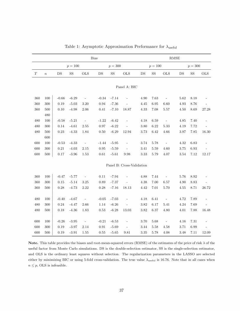
Table 1: Asymptotic Approximation Performance for λuseful

Bias RMSE

p = 100 p = 300 p = 100 p = 300

T n DS SS OLS DS SS OLS DS SS OLS DS SS OLS

Panel A: BIC

360 100 -0.66 -6.29 - -0.34 -7.14 - 4.90 7.63 - 5.62 8.18 -

360 300 0.19 -5.03 3.20 0.94 -7.36 - 4.45 6.95 6.60 4.93 8.76 -

360 500 0.10 -4.98 2.06 0.41 -7.10 18.87 4.33 7.08 5.57 4.50 8.69 27.28

480

480 100 -0.58 -5.21 - -1.22 -6.42 - 4.18 6.59 - 4.85 7.40 -

480 300 0.14 -4.61 2.55 0.97 -6.22 - 3.80 6.22 5.33 4.19 7.72 -

480 500 0.23 -4.33 1.84 0.50 -6.29 12.94 3.73 6.42 4.66 3.97 7.85 16.30

600

600 100 -0.53 -4.33 - -1.44 -5.95 - 3.74 5.78 - 4.32 6.83 -

600 300 0.21 -4.03 2.15 0.95 -5.59 - 3.41 5.59 4.60 3.75 6.93 -

600 500 0.17 -3.96 1.53 0.61 -5.61 9.98 3.33 5.79 4.07 3.54 7.12 12.17

Panel B: Cross-Validation

360 100 -0.47 -5.77 - 0.11 -7.94 - 4.88 7.44 - 5.76 8.92 -

360 300 0.15 -5.14 3.25 0.89 -7.37 - 4.38 7.00 6.57 4.90 8.83 -

360 500 0.28 -4.73 2.22 0.28 -7.16 18.13 4.42 7.01 5.70 4.55 8.71 26.72

480 100 -0.40 -4.67 - -0.05 -7.03 - 4.18 6.41 - 4.72 7.89 -

480 300 0.24 -4.47 2.66 1.14 -6.26 - 3.82 6.17 5.41 4.24 7.69 -

480 500 0.18 -4.36 1.83 0.53 -6.28 13.03 3.82 6.37 4.80 4.01 7.88 16.48

600 100 -0.26 -3.95 - -0.21 -6.53 - 3.70 5.68 - 4.16 7.31 -

600 300 0.19 -3.97 2.14 0.91 -5.69 - 3.44 5.58 4.58 3.71 6.99 -

600 500 0.19 -3.91 1.55 0.55 -5.65 9.81 3.35 5.78 4.08 3.48 7.11 12.09

Note. This table provides the biases and root-mean-squared errors (RMSE) of the estimates of the price of risk λ of the

useful factor from Monte Carlo simulations. DS is the double-selection estimator, SS is the single-selection estimator,

and OLS is the ordinary least squares without selection. The regularization parameters in the LASSO are selected

either by minimizing BIC or using 5-fold cross-validation. The true value λuseful is 16.76. Note that in all cases when

n ≤ p, OLS is infeasible.

37

Table 2: Asymptotic Approximation Performance for λredundant

Bias RMSE

p = 100 p = 300 p = 100 p = 300

T n DS SS OLS DS SS OLS DS SS OLS DS SS OLS

Panel A: BIC

360 100 0.62 -21.11 - -2.38 -25.54 - 14.21 28.02 - 16.74 30.37 -

360 300 -0.17 -13.72 -0.23 -0.12 -13.01 - 5.73 19.47 8.89 6.16 17.32 -

360 500 -0.06 -12.01 -0.11 -0.08 -10.27 -1.08 4.32 17.52 5.98 4.37 14.12 26.99

480 100 0.30 -23.46 - -3.08 -29.92 - 13.58 30.98 - 17.88 34.15 -

480 300 -0.10 -18.07 0.03 -0.04 -16.70 - 5.52 24.25 8.16 5.90 21.50 -

480 500 -0.09 -15.03 -0.18 -0.10 -13.68 -0.46 4.15 21.41 5.46 4.24 18.06 15.42

600 100 0.51 -24.41 - -3.15 -33.22 - 12.85 33.11 - 18.20 36.84 -

600 300 -0.02 -20.79 -0.03 -0.22 -21.10 - 5.33 27.62 7.61 5.62 26.24 -

600 500 -0.14 -18.20 -0.13 -0.07 -16.99 -0.25 3.98 25.18 5.11 3.99 21.75 12.08

Panel B: Cross-Validation

360 100 0.52 -16.95 - -0.97 -21.43 - 12.57 24.64 - 14.65 26.76 -

360 300 -0.23 -14.24 -0.40 -0.04 -12.36 - 5.89 19.97 8.93 6.11 16.55 -

360 500 -0.12 -11.84 -0.17 -0.18 -10.34 -0.44 4.26 17.45 5.91 4.37 14.18 27.01

480 100 0.28 -19.10 - -1.38 -26.45 - 12.14 27.80 - 14.94 30.82 -

480 300 -0.12 -17.78 -0.27 -0.09 -17.00 - 5.55 24.06 8.13 5.79 21.71 -

480 500 -0.21 -15.19 -0.21 -0.04 -13.60 -0.03 4.13 21.58 5.44 4.21 17.87 15.39

600 100 0.28 -20.60 - -0.49 -30.10 - 11.78 29.94 - 14.51 33.93 -

600 300 -0.12 -20.46 -0.30 -0.14 -20.73 - 5.33 27.37 7.63 5.70 25.73 -

600 500 -0.15 -17.77 -0.19 -0.04 -16.64 0.11 4.01 24.86 5.12 4.05 21.46 12.26

Note. This table provides the biases and root-mean-squared errors (RMSE) of the estimates of the price of risk λ of

the redundant factor from Monte Carlo simulations. DS is the double-selection estimator, SS is the single-selection

estimator, and OLS is the ordinary least squares without selection. The regularization parameters in the LASSO are

selected either by minimizing BIC or using 5-fold cross-validation. The true value λredundant is 0. Note that in all cases

when n ≤ p, OLS is infeasible.

38

Table 3: Asymptotic Approximation Performance for λuseless

Bias RMSE

p = 100 p = 300 p = 100 p = 300

T n DS SS OLS DS SS OLS DS SS OLS DS SS OLS

Panel A: BIC

360 100 0.41 -0.23 - 3.70 5.94 - 13.21 15.83 - 16.81 19.36 -

360 300 0.00 -0.05 0.11 0.07 0.61 - 5.89 8.37 9.00 5.92 7.93 -

360 500 0.09 -0.27 0.13 0.01 -0.40 -0.53 4.23 6.78 5.87 4.41 6.11 26.47

480 100 0.24 -0.11 - 5.10 7.67 - 12.60 14.78 - 18.75 21.23 -

480 300 0.10 0.02 0.00 -0.05 0.93 - 5.51 8.39 8.20 5.81 8.17 -

480 500 0.04 -0.32 0.05 0.03 -0.41 0.39 4.03 7.10 5.37 4.20 6.58 14.96

600 100 -0.03 -0.17 - 5.53 8.72 - 11.92 14.58 - 18.95 21.97 -

600 300 0.20 0.17 0.29 -0.12 0.88 - 5.48 8.82 7.65 5.43 8.44 -

600 500 0.01 -0.51 -0.02 -0.04 -0.61 0.05 3.95 7.24 5.06 4.05 6.61 12.19

Panel B: Cross-Validation

360 100 -0.10 -0.63 - 2.03 4.08 - 12.12 14.06 - 15.10 16.75 -

360 300 0.14 0.07 0.09 0.12 0.55 - 5.68 8.09 9.02 6.00 7.74 -

360 500 -0.09 -0.49 -0.12 0.00 -0.22 0.31 4.21 6.88 5.86 4.35 6.02 26.75

480 100 0.07 -0.13 - 2.64 5.26 - 11.41 13.17 - 15.40 17.55 -

480 300 -0.04 -0.05 -0.21 0.09 0.75 - 5.65 8.51 8.23 5.74 8.11 -

480 500 -0.10 -0.40 -0.15 0.03 -0.50 -0.02 4.14 6.99 5.43 4.20 6.42 15.33

600 100 0.05 -0.05 - 3.19 6.23 - 11.01 12.99 - 15.74 18.27 -

600 300 0.02 0.11 0.14 0.13 1.19 - 5.48 8.72 7.68 5.48 8.50 -

600 500 0.03 -0.58 -0.04 0.09 -0.51 -0.10 4.01 7.15 5.17 4.08 6.59 12.02

Note. This table provides the biases and root-mean-squared errors (RMSE) of the estimates of the price of risk λ

of the useless factor from Monte Carlo simulations. DS is the double-selection estimator, SS is the single-selection

estimator, and OLS is the ordinary least squares without selection. The regularization parameters in the LASSO are

selected either by minimizing BIC or using 5-fold cross-validation. The true value λuseless is 0. Note that in all cases

when n ≤ p, OLS is infeasible.

39

Table 4: Testing for Factors Introduced in 2011-2016

(1) (2) (3) (4) (5)

DS SS FF3 No Selection Avg. Ret.

λs tstat λs tstat λs tstat λs tstat avg.ret. tstat

id Factor Description (bp) (DS) (bp) (DS) (bp) (bp) (bp)

84 Maximum Return -50 -0.40 -134 -2.93*** 15 0.43 -291 -1.03 3 0.16

85 Percent Accruals -6 -0.25 17 1.36 -18 -1.81* -34 -0.58 11 1.18

86 Cash Holdings -102 -1.48 52 1.85* 26 1.24 -143 -0.87 19 1.34

87 HML Devil 44 0.53 29 0.44 -108 -2.27** -20 -0.10 27 1.55

88 Gross profitability -22 -0.50 11 0.37 42 2.62*** 50 0.49 21 1.71*

89 Organizational Capital -44 -0.99 -46 -1.67* 46 2.77*** 20 0.23 41 2.67***

90 Betting Against Beta -17 -0.51 -41 -1.61 19 1.02 -22 -0.32 92 5.42***

91 Quality Minus Junk 118 2.84*** 21 0.72 40 2.35** 84 0.95 50 4.09***

92 HXZ Investment 41 1.93* -1 -0.05 -3 -0.27 25 0.58 38 4.15***

93 HXZ Profitability 136 4.00*** 15 0.68 34 2.22** 10 0.18 57 4.51***

94 Employee Growth 14 0.36 -20 -0.92 -2 -0.13 -27 -0.32 7 0.63

95 RMW 122 4.66*** -2 -0.09 22 1.62 105 1.46 36 3.08***

96 CMA 64 2.37** 6 0.31 1 0.05 21 0.37 31 3.23***

97 Intermediary Capital -35 -0.54 -67 -1.00 97 1.86* 92 0.58

98 Intermediary Investment 53 0.65 -71 -0.92 63 0.98 17 0.10 116 3.57***

99 Convertible Debt -10 -0.59 -12 -0.90 6 0.61 -60 -1.70* 7 0.90

Note. The table reports tests for the contribution of factors introduced in 2011-2016 relative to the set of factors

introduced up to 2010. The set of 248 potential controls includes the factors introduced up to and including 2010, their

squares and interactions with size. For each column, we show the estimate of risk price λg and the t-statistic. The first

column uses the double-selection (DS) method, our benchmark. The regularization parameters in each selection are

chosen by 5-fold cross-validation. The second column uses the single-selection (SS) method. The third column uses the

Fama-French 3 factors as controls. The fourth column estimates risk prices using all factors as controls, without using

dimension-reduction techniques, with simple OLS. The last column reports the risk premium of each tradable factor.

Sample period is from July 1980 to December 2016.

40

Table 5: Testing Factors Recursively by Year of Publication

(1) (2) (3)

Year # Assets # Controls New factors (IDs)

1994 450 65 23 24

1995 500 71 25 26 27

1996 500 80 28 29

1997 550 86 30

1998 575 89 31 32 33 34 35 36

1999 725 107 37 38

2000 750 113 39 40 41 42

2001 800 125 43 44 45

2002 825 134 46 47 48

2003 875 143 49 50 51

2004 925 152 52 53 54 55 56

2005 1025 167 57 58 59 60 61

2006 1100 182 62 63 64 65 66 67

2007 1275 203 69 70 71

2008 1350 212 72 73 74 75

2009 1450 224 76 77 78 79

2010 1525 236 80 81 82 83

2011 1625 248 84 85

2012 1675 254 86

2013 1700 257 87 88 89

2014 1750 266 90 91 92 93 94

2015 1825 281 95 96

2016 1825 287 97 98 99

Note. The table reports the results of a recursive factor-testing exercise, from 1994 to 2016. For each year t, column

(1) reports the number of test assets available for the test at that point in time, sorted on characteristics available up

to then. Column (2) reports the number of controls available in each year t, i.e. the number of potential controls in

ht based on factors introduced up to then, plus their squares and interactions with size. Column (3) shows for each

year the IDs of the factors that were introduced during that year. We then test whether each new factor contributes

to explaining asset prices relative to the factors published in previous years, using only the data available up to time

t. We underline the IDs in column (3) every time the factor appears significant using our double-selection test. The

regularization parameters in each selection are chosen by 5-fold cross-validation.

41

Table 6: Robustness for Factors Introduced in 2011-2016

(1) (2) (3) (4) (5)

Bivariate 5× 5 Sequential 5× 5 Pre-1994 Tradable Factors Elastic Net

λs tstat λs tstat λs tstat λs tstat λs tstat

id Factor Description (bp) (DS) (bp) (DS) (bp) (DS) (bp) (DS) (bp) (DS)

84 Maximum Return -50 -0.40 -108 -0.86 -167 -1.19 74 0.60 -103 -0.82

85 Percent Accruals -6 -0.25 -19 -0.81 3 0.12 -38 -1.47 -11 -0.42

86 Cash Holdings -102 -1.48 -143 -2.00** -27 -0.40 59 0.73 -99 -1.40

87 HML Devil 44 0.53 -22 -0.28 -35 -0.43 5 0.07 78 1.03

88 Gross profitability -22 -0.50 -34 -0.77 -41 -0.92 -55 -1.03 -6 -0.11

89 Organizational Capital -44 -0.99 -32 -0.75 -51 -1.20 -67 -1.52 -49 -1.15

90 Betting Against Beta -17 -0.51 -25 -0.73 -42 -1.31 16 0.52 -2 -0.06

91 Quality Minus Junk 118 2.84*** 107 2.60*** 193 4.51*** 31 0.81 91 2.28**

92 HXZ Investment 41 1.93* 48 2.28** 64 2.83*** 48 2.10** 42 1.85*

93 HXZ Profitability 136 4.00*** 121 3.95*** 150 4.20*** 80 2.43** 64 1.88*

94 Employee Growth 14 0.36 52 1.37 -11 -0.31 10 0.26 -2 -0.05

95 RMW 122 4.66*** 117 3.43*** 117 2.77*** 94 2.56*** 111 3.53***

96 CMA 64 2.37** 59 2.27** 74 2.92*** 56 2.02** 19 0.70

97 Intermediary Capital -35 -0.54 -29 -0.48 -16 -0.27 -31 -0.49 -36 -0.47

98 Intermediary Investment 53 0.65 74 0.90 27 0.32 -96 -1.17 -37 -0.40

99 Convertible Debt -10 -0.59 -8 -0.50 13 0.95 14 1.14 6 0.30

Note. The table reports robustness tests for the estimates of risk prices for factors introduced in 2011-2016 relative

to the set of factors introduced up to 2010. The first column shows the same results as in the first column of Table 4

for convenience. The second column shows the results using sequentially-sorted portfolios, the third column uses only

characteristics-sorted portfolios available up to 1994, and the fourth column uses only tradable factors. In the last

column, we use Elastic Net regularization for factor selection instead of LASSO. The regularization parameters in each

selection are chosen by 5-fold cross-validation.

42

Figure 1: Histograms of the Standardized Estimates in Simulations

-5 0 5

0

0.2

0.4

Double-Selection: Useful

-5 0 5

0

0.2

0.4

Single-Selection: Useful

-5 0 5

0

0.2

0.4

Double-Selection: Redundant

-5 0 5

0

0.2

0.4

Single-Selection: Redundant

-5 0 5

0

0.2

0.4

Double-Selection: Useless

-5 0 5

0

0.2

0.4

Single-Selection: Useless

Note. The figure presents the histograms of the standardized double-selection and single-selection estimates using

estimated standard errors, compared with the standard normal density in solid dashed lines. The left panel reports the

double-selection histograms, and the right panel the single-selection histograms. The top row reports the distribution

of standardized estimates for a useful factor; the middle row for a redundant factor; the last row for a useless factor.

In the simulation, we set T = 600, n = 500, and p = 300. The regularization parameters in each selection are chosen

by 5-fold cross-validation.

43

Figure 2: Histograms of the Selected Variables

1st Selection

50 100 150 200 250 300

Factor ID (simulated)

0

0.5

1

Sele

ctio

n r

ate

2nd Selection

50 100 150 200 250 300

Factor ID (simulated)

0

0.5

1

Sele

ctio

n r

ate

Total Selection

50 100 150 200 250 300

Factor ID (simulated)

0

0.5

1

Sele

ctio

n r

ate

Note. The figure reports how often each factor is selected in each step of our double selection procedure (first and

second panels corresponding to the first and second step, and their union in the bottom panel), in Monte Carlo

simulations. Each factor corresponds to a number on the X axis. Factors 1 - 4 are part of the true factors in the DGP.

Factors 5 - 152 are redundant, whereas factors 153 - 300 are useless. We set T = 600, n = 500, and p = 300. The

regularization parameters in each selection are chosen by 5-fold cross-validation.

44

Figure 3: Factors Introduced in 2011-2016: Robustness to Tuning Parameters

Note. The figures provide heat maps for double-selection tests of factors introduced in 2011-2016, as in the first

column of Table 4, using a wide range of tuning parameters, for the first LASSO stage on the X axis and for the second

stage on the Y axis. Each factor corresponds to a row. For each factor, the left panel shows the t-statistics from our

double selection method; the right panel indicates the number of controls selected from ht (the union of the 1st and

2nd selections).

45

46

47

Figure 4: Subsamples: Factor t-statistics

-2 0 2 4

0

0.1

0.2

0.3

0.4

0.5Maximum Return

-2 0 2 4

0

0.1

0.2

0.3

0.4

0.5Percent Accruals

-2 0 2 4

0

0.1

0.2

0.3

0.4

0.5Cash Holdings

-2 0 2 4

0

0.1

0.2

0.3

0.4

0.5HML Devil

-2 0 2 4

0

0.1

0.2

0.3

0.4

0.5Gross profitability

-2 0 2 4

0

0.1

0.2

0.3

0.4

0.5Organizational Capital

-2 0 2 4

0

0.1

0.2

0.3

0.4

0.5Betting Against Beta

-2 0 2 4

0

0.1

0.2

0.3

0.4

0.5Quality Minus Junk

-2 0 2 4

0

0.1

0.2

0.3

0.4

0.5HXZ Investment

-2 0 2 4

0

0.1

0.2

0.3

0.4

0.5HXZ Profitability

-2 0 2 4

0

0.1

0.2

0.3

0.4

0.5Employee Growth

-2 0 2 4

0

0.1

0.2

0.3

0.4

0.5RMW

-2 0 2 4

0

0.1

0.2

0.3

0.4

0.5CMA

-2 0 2 4

0

0.1

0.2

0.3

0.4

0.5Intermediary Capital

-2 0 2 4

0

0.1

0.2

0.3

0.4

0.5Intermediary Investment

-2 0 2 4

0

0.1

0.2

0.3

0.4

0.5Convertible Debt

Note. The figure reports the histogram of individual factor t-statistics estimates across 2,000 bootstrap samples, for the

factors introduced since 2011 (as in Table 4). We bootstrap our data over both the time-series and the cross-sectional

(test assets) dimensions.

48

Figure 5: Subsamples: Factor Selection Rate

0 50 100 150 200 250

Factor ID

0

0.1

0.2

0.3

0.4

0.5

0.6

0.7

0.8

Sele

ction r

ate

Note. The figure reports the control factor selection rates for the tests of Table 4 (i.e., the factors selected by the first

LASSO step of the double-selection procedure), across bootstrap samples selected as in Figure 4. The figure shows,

for each factor identified by the factor ID (on the X axis), in what fraction of the 2,000 samples that factor is selected

by LASSO. The first 83 factors are the original factors; the next 83 factors are the squared factors and the last 82 are

their interaction with Small Minus Big.

49

Appendix A List of Factors

Table A.1: Factor Zoo

id Category Description Year Avg.Ret Annual S.R. Reference

1 V Excess Market Return 1965 0.65% 50.61% Sharpe (1964)

2 T Beta 1973 -0.18% -10.71% Fama and MacBeth (1973)

3 V Earnings to Price 1977 0.20% 21.79% Basu (1977)

4 V Dividend to Price 1982 0.12% 9.02% Litzenberger and Ramaswamy (1982)

5 M Unexpected Quarterly Earnings 1982 0.04% 7.90% Rendleman et al. (1982)

6 V Long-Term Reversal 1985 0.19% 26.54% Bondt and Thaler (1985)

7 V Leverage 1988 0.12% 13.39% Bhandari (1988)

8 T Bid-Ask Spread 1989 0.12% 8.27% Amihud and Mendelson (1989)

9 IN Cash Flow to Debt 1989 0.06% 12.17% Ou and Penman (1989)

10 IN Current Ratio 1989 -0.01% -0.49% Ou and Penman (1989)

11 IN Change in Current Ratio 1989 0.05% 14.00% Ou and Penman (1989)

12 IN Change in Quick Ratio 1989 0.03% 6.80% Ou and Penman (1989)

13 IN Change Sales-to-Inventory 1989 0.03% 7.28% Ou and Penman (1989)

14 IN Quick Ratio 1989 0.00% 0.03% Ou and Penman (1989)

15 IN Sales to Cash 1989 -0.04% -4.72% Ou and Penman (1989)

16 IN Sales to Inventory 1989 -0.01% -1.65% Ou and Penman (1989)

17 IN Sales to Receivables 1989 0.15% 22.42% Ou and Penman (1989)

18 V Depreciation / PP&E 1992 0.11% 10.83% Holthausen and Larcker (1992)

19 V Change in Depreciation 1992 0.05% 11.90% Holthausen and Larcker (1992)

20 T Small Minus Big 1993 0.12% 14.11% Fama and French (1993)

21 V High Minus Low 1993 0.32% 37.11% Fama and French (1993)

22 T Short-Term Reversal 1993 0.29% 29.95% Jegadeesh and Titman (1993)

23 P Industry-Adjusted Change in Employees 1994 -0.01% -2.71% Asness et al. (2000)

Note. The factor zoo contains 98 tradable and 1 nontradable (No.97) factors for monthly data from July 1980 to

December 2016. In addition to these publicly available factors, we follow Fama and French (1993) to construct value-

weighted portfolios as factors using firm characteristics collected in Green et al. (2016). For each characteristic therein,

we sort all stocks into deciles based on their previous year-end values, then build and rebalance a long-short portfolio

(top 30% - bottom 30% or 1-0 dummy difference) every June. For factor classification, “M” is Momentum, “V” is

Value-versus-Growth, “I” is Investment, “P” is Profitability, “IN” is Intangibles, and “T” is Trading Frictions.

50

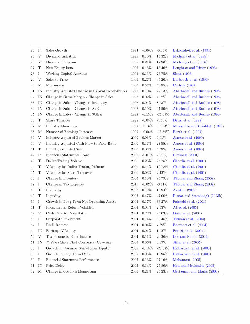
24 P Sales Growth 1994 -0.06% -8.34% Lakonishok et al. (1994)

25 V Dividend Initiation 1995 0.16% 14.32% Michaely et al. (1995)

26 V Dividend Omission 1995 0.21% 17.93% Michaely et al. (1995)

27 T New Equity Issue 1995 0.15% 13.46% Loughran and Ritter (1995)

28 I Working Capital Accruals 1996 0.13% 25.75% Sloan (1996)

29 V Sales to Price 1996 0.27% 35.26% Barbee Jr et al. (1996)

30 M Momentum 1997 0.57% 43.95% Carhart (1997)

31 IN Industry Adjusted Change in Capital Expenditures 1998 0.10% 22.13% Abarbanell and Bushee (1998)

32 IN Change in Gross Margin - Change in Sales 1998 0.02% 4.32% Abarbanell and Bushee (1998)

33 IN Change in Sales - Change in Inventory 1998 0.04% 8.63% Abarbanell and Bushee (1998)

34 IN Change in Sales - Change in A/R 1998 0.19% 47.59% Abarbanell and Bushee (1998)

35 IN Change in Sales - Change in SG&A 1998 -0.13% -26.65% Abarbanell and Bushee (1998)

36 T Share Turnover 1998 -0.05% -4.40% Datar et al. (1998)

37 M Industry Momentum 1999 -0.13% -13.23% Moskowitz and Grinblatt (1999)

38 M Number of Earnings Increases 1999 -0.06% -15.80% Barth et al. (1999)

39 V Industry-Adjusted Book to Market 2000 0.06% 9.91% Asness et al. (2000)

40 V Industry-Adjusted Cash Flow to Price Ratio 2000 0.17% 27.98% Asness et al. (2000)

41 T Industry-Adjusted Size 2000 0.03% 4.59% Asness et al. (2000)

42 P Financial Statements Score 2000 -0.01% -1.53% Piotroski (2000)

43 T Dollar Trading Volume 2001 0.23% 25.75% Chordia et al. (2001)

44 T Volatility for Dollar Trading Volume 2001 0.14% 19.78% Chordia et al. (2001)

45 T Volatility for Share Turnover 2001 0.03% 2.12% Chordia et al. (2001)

46 I Change in Inventory 2002 0.13% 24.79% Thomas and Zhang (2002)

47 I Change in Tax Expense 2011 -0.02% -3.41% Thomas and Zhang (2002)

48 T Illiquidity 2002 0.19% 19.94% Amihud (2002)

49 T Liquidity 2003 0.47% 47.00% Pastor and Stambaugh (2003b)

50 I Growth in Long Term Net Operating Assets 2003 0.17% 36.27% Fairfield et al. (2003)

51 T Idiosyncratic Return Volatility 2003 0.04% 2.43% Ali et al. (2003)

52 V Cash Flow to Price Ratio 2004 0.22% 25.03% Desai et al. (2004)

53 I Corporate Investment 2004 0.14% 30.45% Titman et al. (2004)

54 I R&D Increase 2004 0.04% 7.89% Eberhart et al. (2004)

55 IN Earnings Volatility 2004 0.01% 1.42% Francis et al. (2004)

56 V Tax Income to Book Income 2004 0.11% 20.26% Lev and Nissim (2004)

57 IN # Years Since First Compustat Coverage 2005 0.06% 6.09% Jiang et al. (2005)

58 I Growth in Common Shareholder Equity 2005 -0.15% -23.68% Richardson et al. (2005)

59 I Growth in Long-Term Debt 2005 0.06% 10.95% Richardson et al. (2005)

60 P Financial Statement Performance 2005 0.13% 27.16% Mohanram (2005)

61 IN Price Delay 2005 0.14% 25.89% Hou and Moskowitz (2005)

62 M Change in 6-Month Momentum 2006 0.21% 25.23% Gettleman and Marks (2006)

51

63 I Growth in Capital Expenditures 2006 0.09% 16.10% Anderson and Garcia-Feijoo (2006)

64 IN Industry Sales Concentration 2006 -0.02% -2.57% Hou and Kimmel (2006)

65 I R&D to Market Capitalization 2006 0.37% 40.73% Guo et al. (2006)

66 I R&D to Sales 2006 0.08% 7.67% Guo et al. (2006)

67 T Return Volatility 2006 0.08% 5.72% Ang et al. (2006)

68 T Zero Trading Days 2006 -0.03% -2.11% Liu (2006)

69 M Abnormal Earnings Announcement Volume 2007 0.07% 10.16% Lerman et al. (2008)

70 I Return on Invested Capital 2007 0.17% 26.53% Brown and Rowe (2007)

71 IN Debt Capacity / Firm Tangibility 2007 0.01% 1.31% Almeida and Campello (2007)

72 P Industry-Adjusted Change in Asset Turnover 2008 0.08% 21.65% Soliman (2008)

73 I Change in Shares Outstanding 2008 0.17% 26.20% Pontiff and Woodgate (2008)

74 P Industry-Adjusted Change in Profit Margin 2008 0.11% 19.12% Soliman (2008)

75 M Earnings Announcement Return 2008 -0.01% -2.48% Brandt et al. (2008)

76 V Cash Productivity 2009 0.31% 36.72% Chandrashekar and Rao (2009)

77 M Revenue Surprise 2009 0.13% 19.19% Kama (2009)

78 T Sin Stocks 2009 0.40% 37.15% Hong and Kacperczyk (2009)

79 T Cash Flow Volatility 2009 0.14% 21.22% Huang (2009)

80 IN Absolute Accruals 2010 0.05% 8.82% Bandyopadhyay et al. (2010)

81 IN Capital Expenditures and Inventory 2010 0.17% 29.95% Chen and Zhang (2010)

82 P Return on Assets 2010 0.13% 19.68% Balakrishnan et al. (2010)

83 T Accrual Volatility 2010 0.12% 19.36% Bandyopadhyay et al. (2010)

84 T Maximum Daily Return 2011 0.03% 2.71% Bali et al. (2011)

85 IN Percent Accruals 2011 0.11% 19.54% Hafzalla et al. (2011)

86 IN Cash Holdings 2012 0.19% 22.22% Palazzo (2012)

87 V HML Devil 2013 0.27% 25.71% Asness and Frazzini (2013)

88 P Gross Profitability 2013 0.21% 28.32% Novy-Marx (2013)

89 IN Organizational Capital 2013 0.41% 44.25% Eisfeldt and Papanikolaou (2013)

90 T Betting Against Beta 2014 0.92% 89.71% Frazzini and Pedersen (2014)

91 V Quality Minus Junk 2014 0.50% 67.63% Asness et al. (2014)

92 I HXZ Investment 2014 0.38% 68.72% Hou et al. (2014)

93 P HXZ Profitability 2014 0.57% 74.64% Hou et al. (2014)

94 I Employee Growth Rate 2014 0.07% 10.40% Belo et al. (2014)

95 P Robust Minus Weak 2015 0.36% 50.97% Fama and French (2015)

96 I Conservative Minus Aggressive 2015 0.31% 53.52% Fama and French (2015)

97 T Intermediary Capital Risk 2016 He et al. (2016)

98 T Intermediary Investment 2016 1.16% 59.07% He et al. (2016)

99 IN Convertible Debt Indicator 2016 0.07% 14.82% Valta (2016)

52

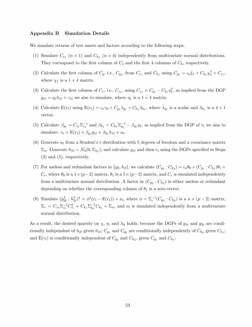
Appendix B Simulation Details

We simulate returns of test assets and factors according to the following steps:

(1) Simulate Ce1 (n × 1) and Ch1 (n × 4) independently from multivariate normal distributions.

They correspond to the first column of Ce and the first 4 columns of Ch, respectively.

(2) Calculate the first column of Cg, i.e., Cg1 , from Ce1 and Ch1 using Cg1 = ιnξ1 + Ch1χᵀ1 + Ce1 ,

where χ1 is a 1× 4 matrix.

(3) Calculate the first column of Cz, i.e., Cz1 , using Cz1 = Cg1 − Ch1ηᵀ1 , as implied from the DGP

g1t = η1h1t + z1t we aim to simulate, where η1 is a 1× 4 matrix.

(4) Calculate E(rt) using E(rt) = ιnγ0 + Cg1λg1 + Ch1λh1 , where λg1 is a scalar and λh1 is a 4× 1

vector.

(5) Calculate βg1 = Cz1Σ−1z1 and βh1 = Ch1Σ−1h1 − βg1η1, as implied from the DGP of rt we aim to

simulate: rt = E(rt) + βg1g1t + βh1h1t + ut.

(6) Generate ut from a Student’s t distribution with 5 degrees of freedom and a covariance matrix

Σu. Generate h1t ∼ N4(0,Σh1), and calculate g1t and then rt using the DGPs specified in Steps

(3) and (5), respectively.

(7) For useless and redundant factors in {g2, h2}, we calculate (Cg2 : Ch2) = ιnθ0 + (Cg1 : Ch1)θ1 +

Cε, where θ0 is a 1×(p−2) matrix, θ1 is a 5×(p−2) matrix, and Cε is simulated independently

from a multivariate normal distribution. A factor in (Cg2 : Ch2) is either useless or redundant

depending on whether the corresponding column of θ1 is a zero-vector.

(8) Simulate (gᵀ2t : hᵀ2t)ᵀ = φᵀ(rt − E(rt)) + νt, where φ = Σ−1r (Cg2 : Ch2) is a n × (p − 2) matrix,

Σr = Cz1Σ−1z1 Cᵀz1 + Ch1Σ−1h1 Ch1 + Σu, and νt is simulated independently from a multivariate

normal distribution.

As a result, the desired sparsity on χ, η, and λh holds, because the DGPs of g1t and g2t are condi-

tionally independent of h2t given h1t; Cg1 and Cg2 are conditionally independently of Ch2 given Ch1 ;

and E(rt) is conditionally independent of Cg2 and Ch2 , given Cg1 and Ch1 .

53

Online Appendix A Technical Details and Proofs

A.1 Notation

We summarize the notation used throughout. Let ei be a vector with 1 in the ith entry and 0

elsewhere, whose dimension depends on the context. Let ιk denote a k-dimensional vector with all

entries being 1. We use a∨b to denote the max of a and b, and a∧b as their min for any scalars a and

b. We also use the notation a . b to denote a ≤ Kb for some constant K > 0; and a .p b to denote

a = Op(b). For any time series of vectors {at}Tt=1, we denote a = T−1∑T

t=1 at. In addition, we write

at = at−a. We use the capital letter A to denote the matrix (a1 : a2 : . . . : aT ), and write A = A−ιᵀT acorrespondingly. We use λmin(A) and λmax(A) to denote the minimum and maximum eigenvalues of

A. We use ‖A‖1, ‖A‖∞, ‖A‖, and ‖A‖F to denote the L1 norm, the L∞ norm, the operator norm

(or L2 norm), and the Frobenius norm of a matrix A = (aij), that is, maxj∑

i |aij |, maxi∑

j |aij |,√λmax(AᵀA), and

√Tr(AᵀA), respectively. We also use ‖A‖MAX = maxi,j |aij | to denote the L∞

norm of A on the vector space. When a is a vector, both ‖a‖ and ‖a‖F are equal to its Euclidean

norm. We use ‖a‖0 to denote∑

i 1{ai 6=0}. We also denote Supp(a) = {i : ai 6= 0}. We write

the projection operator with respect to a matrix A as PA = A(AᵀA)−1Aᵀ, and the corresponding

annihilator as MA = I− PA, where I is the identity matrix whose size depends on the context. For

a set of indices I, let A[I] denote a sub-matrix of A, which contains all columns indexed in I.

A.2 Technical Assumptions

Assumption A.1 (Sparsity). ‖λh‖0 ≤ s, ‖χj,·‖0 ≤ s, ‖ηj,·‖0 ≤ s, 1 ≤ j ≤ d, for some s such that

sn−1 → 0.

Definition 1 (LASSO and Post-LASSO Estimators). We consider a generic linear regression prob-

lem with sparse coefficients:

Y = Xβ + ε, subject to ‖β‖0 ≤ s,

where Y is a n × 1 vector, X is a n × p matrix, β is p × 1 vector of parameters. We define the

LASSO estimator as

β = arg minβ

{n−1 ‖Y −Xβ‖2 + n−1τ ‖β‖1

}.

We define the Post-LASSO estimator βI

as

βI

= arg minβ

{n−1 ‖Y −Xβ‖2 : βj = 0, j /∈ I

},

where I is the set of indices of variables selected by a first-step LASSO, that is, I = Supp(β).

54

We adopt a high-level assumption on the model selection properties of LASSO and the prediction

error bounds of the Post-LASSO estimators in (7) and (8). Belloni and Chernozhukov (2013) provide

more primitive conditions for these bounds to hold.

Assumption A.2 (Properties of Post-LASSO Estimators). The Post-LASSO estimators in (7) and

(8) satisfy the following properties:

1. s = |I1⋃I2| .p s.

2. Moreover, if τ0 ≥ 2c∥∥∥λᵀgCᵀ

e (ιn : Ch)∥∥∥1, for some c > 1, then

n−1/2∥∥∥ιn(γ

I1− γ0) + Ch(λ

I1− λh)

∥∥∥ .p sT−1/2(log(n ∨ p ∨ T ))1/2 + τ0s

1/2n−1, (A.1)

where γ0 = γ0 + ξᵀλg and λh = χᵀλg + λh are the true parameter values given in (2) and (6).

If τj ≥ 2cj

∥∥∥eᵀjCᵀe (ιn : Ch)

∥∥∥1, for some cj > 1 and j = 1, 2, . . . , d, then

n−1/2∥∥∥ιn(ξ

I2− ξ)ᵀ + Ch(χ

I2− χ)ᵀ

∥∥∥ .p sT−1/2(log(n ∨ p ∨ T ))1/2 + ‖τ‖MAX s

1/2n−1, (A.2)

where τ = (τ1, τ2, . . . , τd)ᵀ, ξ and χ are the true parameter values given in (6).

Assumption A.2 gives a probabilistic upper bound on s. The prediction error bounds in (A.1)

and (A.2) are more conservative than the standard results, because the regressors here are estimated.

We provide a sketch of the proof for (A.1) in Appendix A.4, for which we need the following sparse

eigenvalues assumption. The proof of (A.2) is similar and simpler. Our theoretical result below

would also hold if other model selection procedures are employed, provided that they obey similar

properties in Assumption A.2.

Assumption A.3 (Sparse Eigenvalues). There exist K1,K2 > 0 and a sequence ln →∞, such that

with probability approaching 1,

K1 ≤ φmin(lns)[n−1(ιn : Ch)ᵀ(ιn : Ch)

]≤ φmax(lns)

[n−1(ιn : Ch)ᵀ(ιn : Ch)

]≤ K2,

where we denote

φmin(k)[A] = min1≤‖v‖0≤k

vᵀAv

‖v‖2, and φmax(k)[A] = max

1≤‖v‖0≤k

vᵀAv

‖v‖2.

Assumption A.3 resembles one of the sufficient conditions that lead to desirable statistical

properties of LASSO, which has been adopted by, e.g., Belloni et al. (2014b). It implies the restricted

eigenvalue condition proposed by Bickel et al. (2009).

Assumption A.4 (Large Deviation Bounds). The stochastic discount factor, the returns, and the

factors satisfy

‖a‖MAX .p T−1/2(log(n ∨ p ∨ T ))1/2, where a ∈ {m, v, z, u}. (A.3)∥∥T−1ABᵀ − Cov(at, bt)

∥∥MAX

.p T−1/2(log(n ∨ p ∨ T ))1/2, where A,B ∈ {M,V,Z, U}. (A.4)

55

Assumption A.4 imposes high-level assumptions on the large deviation type bounds, which can

be verified using the same arguments as in Fan et al. (2011) under stationarity, ergodicity, strong

mixing, and exponential-type tail conditions.

Next, we impose additional uniform bounds that impose restrictions on the cross-sectional

dependence of the “residuals” in the covariance projection (6). Similar assumptions on factor loadings

are employed by Giglio and Xiu (2016).

Assumption A.5 (“Moment” Conditions). The following restrictions hold:

‖Ce‖MAX . 1, ‖Cᵀe ιn‖MAX . n1/2, ‖Cᵀ

eCh‖MAX . n1/2, (A.5)

‖Cᵀe u‖MAX .p n

1/2T−1/2,∥∥Cᵀ

e U Vᵀ∥∥MAX

.p n1/2T 1/2, (A.6)

λmin(n−1CᵀeCe) ≥ K, ‖Cᵀ

e (βgη + βh)‖∞ . sn1/2, ‖βh‖∞ . s. (A.7)

In addition, for a ∈ {m, v, z, u}, it holds that

‖Σa‖MAX . 1, ‖Ca‖MAX . 1. (A.8)

Finally, we impose a joint central limit theorem for (zt, λᵀvtzt) = (zt, (1 − γ0mt)zt). This can

be verified by the standard central limit theory for dependent stochastic processes, if more primitive

assumptions are satisfied, see, e.g., White (2000).

Assumption A.6 (CLT). The following results hold as T →∞:

T 1/2

(z

−T−1γ0MZ − Σzλg

)L−→ N

((0

0

),

(Π11 Π12

Πᵀ12 Π22

)),

where Π11, Π12, and Π22 are given by

Π11 = limT→∞

1

T

T∑t=1

T∑s=1

E(zszᵀt ),

Π12 = limT→∞

1

T

T∑t=1

T∑s=1

E (λᵀvszszᵀt ) ,

Π22 = limT→∞

1

T

T∑t=1

T∑s=1

E (λᵀvsλᵀvtzsz

ᵀt ) .

Assumption A.7 (Selection for the Asymptotic Variance Estimator). The Post-LASSO estimator

ηI

satisfies the usual bounds. That is, if τj ≥ 2cj ‖HZ‖∞, for some cj > 1, j = 1, 2, . . . , d, then we

have ∥∥(ηI− η)H

∥∥ .p s1/2(log(p ∨ T ))1/2, and

∥∥ηI− η∥∥ .p s

1/2T−1/2(log(p ∨ T ))1/2.

56

A.3 Proof of Main Theorems

Proof of Theorem 1. The estimator of λg can be written in closed-form as

λg =(CᵀgM(ιn:Ch[I])

Cg

)−1 (CᵀgM(ιn:Ch[I])

r). (A.9)

Moreover, by (2) and (5), we can relate Cg and Ch to βg and βh:

Cg = Chηᵀ + Cz, where Ch = (βgη + βh)Σh, Cz = βgΣz. (A.10)

Using (3), (5), (A.10), and the fact that

Cg − Cg = (Ch − Ch)ηᵀ + (Cz − Cz),

Cz − Cz = βg(T−1ZZᵀ − Σz

)+ T−1U Zᵀ + T−1 (βgη + βh) HZᵀ,

Ch − Ch = (βgη + βh)(T−1HHᵀ − Σh

)+ T−1UHᵀ + T−1βgZH

ᵀ,

we obtain the following decomposition:

T 1/2(λg − λg)

=(n−1Cᵀ

gM(ιn:Ch[I])Cg

)−1n−1T 1/2Cᵀ

gM(ιn:Ch[I])

((Cg − Cg)λg + Chλh + βg z + ((βgη + βh)h+ u)

)=T 1/2Σ−1z

(z −

(T−1ZV ᵀλ− Σzλg

))+(n−1Cᵀ

gM(ιn:Ch[I])Cg

)−1 (n−1T 1/2Cᵀ

gM(ιn:Ch[I])

(u− T−1U V ᵀλ

)+n−1T 1/2Cᵀ

gM(ιn:Ch[I])(βg − CgΣ−1z )×

(z −

(T−1ZV ᵀλ− Σzλg

))−n−1T 1/2Cᵀ

gM(ιn:Ch[I])(βgη + βh)

(T−1HV ᵀλ− Σh(ηᵀλg + λh)− h

)+n−1T 1/2Cᵀ

gM(ιn:Ch[I])Chλh

).

We first analyze the leading term. Note that γ0M = −V ᵀλ, by Assumption A.6 and applying the

Delta method, we have

T 1/2(Σ−1z z − Σ−1z

(−T−1γ0ZM − Σzλg

))L−→ N

(0, limT→∞

1

T

T∑t=1

T∑s=1

E((1− λᵀvt)(1− λᵀvs)Σ−1z ztz

ᵀsΣ−1z

)). (A.11)

Next, we show that the reminder terms are of a smaller order. By (A.42), we have

n−1T 1/2∥∥∥Cᵀ

gM(ιn:Ch[I])

(u− T−1U V ᵀλ

)∥∥∥ .p s(n−1/2 + T−1/2) log(n ∨ p ∨ T ).

By (A.27), we have

n−1T 1/2∥∥∥Cᵀ

gM(ιn:Ch[I])Chλh

∥∥∥ .p s2(n−1T 1/2 + T−1/2) log(n ∨ p ∨ T ).

57

By (A.40), we have

n−1T 1/2∥∥∥Cᵀ

gM(ιn:Ch[I])(βgη + βh)

(T−1HV ᵀλ− Σh(ηᵀλg + λh)− h

)∥∥∥.ps

2(n−1/2 + T−1/2) log(n ∨ p ∨ T ).

By Assumption A.4, (A.11), and (A.35), we have

n−1T 1/2∥∥∥Cᵀ

gM(ιn:Ch[I])(βg − CzΣ−1z )

(z −

(T−1ZV ᵀλ− Σzλg

))∥∥∥≤n−1T 1/2

∥∥∥CᵀgM(ιn:Ch[I])

(βg − CzΣ−1z )∥∥∥∥∥z − (T−1ZV ᵀλ− Σzλg

)∥∥.ps(n

−1/2 + T−1/2) log(n ∨ p ∨ T ).

This concludes the proof.

Proof of Theorem 2. By the identical argument in the proof of Theorem 2 of Newey and West (1987),

we have

1

T

T∑t=1

T∑r=1

Qtr(1− λᵀvt)(1− λᵀvr) (ztzᵀr + zrz

ᵀt )

p−→ ΣzΠΣz.

So applying the continuous mapping theorem, it is sufficient to show that

Σzp−→ Σz, (A.12)

Π− 1

T

T∑t=1

T∑r=1

Qtr(1− λᵀvt)(1− λᵀvr) (ztzᵀr + zrz

ᵀt )

p−→ 0, (A.13)

where

Qtr =

(1− |r − t|

q + 1

)1{|t−r|≤q}, Π = ΣzΠΣz.

To prove (A.15), we note that by Assumptions A.4 and A.7, we have∥∥∥Σz − Σz

∥∥∥MAX

.T−1/2∥∥(η

I− η)H

∥∥ ‖Z‖MAX + T−1∥∥(η

I− η)H

∥∥2 +∥∥T−1ZZᵀ − Σz

∥∥MAX

.ps1/2T−1/2(log(p ∨ T ))1/2 ‖Z‖MAX + sT−1 log(p ∨ T ) + T−1/2(log(n ∨ p ∨ T ))1/2

=op(1). (A.14)

As to (A.13), we can decompose its left-hand side as

1

T

T∑t=1

T∑r=1

Qtr(λ− λ)ᵀvt(1− λᵀvr) (ztzᵀr + zrz

ᵀt ) (A.15)

58

+1

T

T∑t=1

T∑r=1

Qtr(1− λᵀvt)(λ− λ)ᵀvr (ztzᵀr + zrz

ᵀt ) (A.16)

+1

T

T∑t=1

T∑r=1

Qtr(1− λᵀvt)(1− λᵀvr) ((zt − zt) zᵀr + (zr − zr) zᵀt ) (A.17)

+1

T

T∑t=1

T∑r=1

Qtr(1− λᵀvt)(1− λᵀvr) (zt (zr − zr)ᵀ + zr (zt − zt)ᵀ) . (A.18)

Analyzing each of these terms, we can obtain that∥∥∥∥∥ 1

T

T∑t=1

T∑r=1

Qtr(λ− λ)ᵀvt(1− λᵀvr) (ztzᵀr + zrz

ᵀt )

∥∥∥∥∥MAX

.qT−1∥∥∥Z∥∥∥∥∥∥ιᵀT − λᵀV ∥∥∥∥∥∥(λ− λ)ᵀV

∥∥∥MAX

∥∥∥Z∥∥∥MAX

.p qs1/2(T−1/2 + n−1/2) ‖V ‖MAX ‖Z‖MAX ,∥∥∥∥∥ 1

T

T∑t=1

T∑r=1

Qtr(1− λᵀvt)(λ− λ)ᵀvr (ztzᵀr + zrz

ᵀt )

∥∥∥∥∥MAX

.qT−1∥∥ιᵀT − λᵀV ∥∥∥∥∥Z∥∥∥∥∥∥(λ− λ)ᵀV

∥∥∥MAX

∥∥∥Z∥∥∥MAX

.p qs1/2(T−1/2 + n−1/2) ‖V ‖MAX ‖Z‖MAX ,∥∥∥∥∥ 1

T

T∑t=1

T∑r=1

Qtr(1− λᵀvt)(1− λᵀvr) ((zt − zt) zᵀr + (zr − zr) zᵀt )

∥∥∥∥∥MAX

.qT−1∥∥ιᵀT − λᵀV ∥∥ ‖(η − η)H‖

∥∥∥Z∥∥∥MAX

∥∥ιᵀT − λᵀV ∥∥MAX

.pqs3/2(T−1/2 + n−1/2) ‖V ‖MAX ‖Z‖MAX ,

where we use∥∥ιᵀT − λᵀV ∥∥ . T 1/2 +∥∥M∥∥+ ‖λᵀv‖ .p T

1/2,∥∥ιᵀT − λᵀV ∥∥MAX. 1 + ‖λᵀV ‖MAX . s ‖V ‖MAX ,∥∥∥ιᵀT − λᵀV ∥∥∥ ≤ ∥∥ιᵀT − λᵀV ∥∥+

∥∥∥(λ− λ)ᵀV∥∥∥ .p T

1/2 +∥∥∥λ− λ∥∥∥ ‖V ‖ .p T

1/2,∥∥∥Z∥∥∥ . T 1/2∥∥∥Σz

∥∥∥1/2 .p T1/2 ‖Σz‖1/2 . T 1/2,∥∥∥(λ− λ)ᵀV

∥∥∥MAX

≤∥∥∥λ− λ∥∥∥

∞‖V ‖MAX ≤

∥∥∥λ− λ∥∥∥ ‖V ‖MAX .p s1/2(T−1/2 + n−1/2) ‖V ‖MAX ,∥∥∥Z∥∥∥

MAX≤ ‖(η − η)H‖+ ‖Z‖MAX .p ‖Z‖MAX ,

which hold by (A.14), Assumption A.4, and Lemma 7. This concludes the proof.

A.4 Proof of Lemmas

Proof of (A.1). We provide a sketch of the proof, as they are identical to Belloni and Chernozhukov

(2013). With respect to the optimization problem (7), we define

Q(γ, λ) = n−1∥∥∥r − ιnγ − Chλ∥∥∥2 .59

We denote the solution to this problem as γ and λ. Let δ = λ− λh. Note by (5) and (2), we have

E(rt) = ιnγ0 + Chλh + Ceλg, and r = E(rt) + βg g + βhh+ u.

By direct calculations, we have

Q(γ, λ)−Q(γ0, λh)− n−1∥∥∥ιn(γ − γ0) + Chδ

∥∥∥2=− 2n−1

(r − ιnγ0 − Chλh

)ᵀ (ιn(γ − γ0) + Chδ

)=− 2n−1

(βg g + βhh+ u+ (Ch − Ch)λh + Ceλg

)ᵀ (ιn(γ − γ0) + Chδ

)≥− 2n−1

∥∥∥βg g + βhh+ u+ (Ch − Ch)λh

∥∥∥∥∥∥ιn(γ − γ0) + Chδ∥∥∥

− 2n−1∥∥∥(Ceλg)

ᵀ (ιn : Ch)∥∥∥1‖(γ − γ0 : δᵀ)ᵀ‖1

≥− 2n−1∥∥∥βg g + βhh+ u+ (Ch − Ch)λh

∥∥∥∥∥∥ιn(γ − γ0) + Chδ∥∥∥

− τ0K−1n−1 (|γ − γ0|+ ‖δI‖1 + ‖δIc‖1) ,

where I is the set of non-zeros in λh, Ic is its complement, and δI is a sub-vector of δ with all entries

taken from I.

On the other hand, by definition of γ and λ, we have

Q(γ, λ)−Q(γ0, λh) ≤τ0n−1(∥∥∥(γ0 : λᵀh)ᵀ

∥∥∥1−∥∥∥(γ : λᵀ)ᵀ

∥∥∥1

)≤τ0n−1(|γ − γ0|+ ‖δI‖1 − ‖δIc‖1).

Therefore, we obtain

n−1∥∥∥ιn(γ − γ0) + Chδ

∥∥∥2 − τ0c−1n−1 (|γ − γ0|+ ‖δI‖1 + ‖δIc‖1)

− 2n−1∥∥∥βg g + βhh+ u+ (Ch − Ch)λh

∥∥∥∥∥∥ιn(γ − γ0) + Chδ∥∥∥

≤τ0n−1(|γ − γ0|+ ‖δI‖1 − ‖δIc‖1), (A.19)

where we use the fact that

τ0 ≥ 2c∥∥∥λᵀgCᵀ

e (ιn : Ch)∥∥∥1.

If it holds that

n−1∥∥∥ιn(γ − γ0) + Chδ

∥∥∥− 2n−1∥∥∥βg g + βhh+ u+ (Ch − Ch)λh

∥∥∥ < 0,

we can establish that

n−1/2∥∥∥ιn(γ − γ0) + Chδ

∥∥∥ .p sT−1/2(log(n ∨ p ∨ T ))1/2,

60

where we use the fact that

n−1/2 ‖βg g‖ . ‖βg‖MAX ‖g‖MAX .p T−1/2, (A.20)

n−1/2 ‖u‖ . ‖u‖MAX .p T−1/2(log(n ∨ p ∨ T ))1/2, (A.21)

n−1/2∥∥βhh∥∥ ≤‖βh‖∞ ∥∥h∥∥MAX

.p sT−1/2(log(n ∨ p ∨ T ))1/2, (A.22)

n−1/2∥∥∥(Ch − Ch)λh

∥∥∥ .∥∥∥Ch − Ch∥∥∥

MAX

∥∥∥λh∥∥∥1.p sT

−1/2(log(n ∨ p ∨ T ))1/2. (A.23)

Otherwise, from (A.19) it follows that

−c−1 (|γ − γ0|+ ‖δI‖1 + ‖δIc‖1) ≤ |γ − γ0|+ ‖δI‖1 − ‖δIc‖1 ,

which leads to, writing c = (c+ 1)(c− 1)−1,

‖δIc‖ ≤ c(|γ − γ0|+ ‖δI‖1).

Then by (A.19) again as well as the restricted eigenvalue condition in Belloni and Chernozhukov

(2013), we obtain∥∥∥ιn(γ − γ0) + Chδ∥∥∥2 − 2

∥∥∥βg g + βhh+ u+ (Ch − Ch)λh

∥∥∥∥∥∥ιn(γ − γ0) + Chδ∥∥∥

≤(1 + c−1)τ0(|γ − γ0|+ ‖δI‖1) . τ0s1/2n−1/2

∥∥∥ιn(γ − γ0) + Chδ∥∥∥ .

Therefore, we have

n−1/2∥∥∥ιn(γ − γ0) + Chδ

∥∥∥ .n−1/2∥∥∥βg g + βhh+ u+ (Ch − Ch)λh

∥∥∥+ τ0s1/2n−1

.psT−1/2(log(n ∨ p ∨ T ))1/2 + τ0s

1/2n−1.

The Post-LASSO estimator converges at the same rate following the same arguments as in Belloni

and Chernozhukov (2013).

Lemma 1. Under Assumptions A.1, A.2, A.4, A.5, we have

n−1/2∥∥∥M(ιn:Ch[I])

Chχᵀ∥∥∥ .ps(n

−1/2 + T−1/2)(log(n ∨ p ∨ T ))1/2. (A.24)

n−1/2∥∥∥M(ιn:Ch[I])

Chλh

∥∥∥ .ps(n−1/2 + T−1/2)(log(n ∨ p ∨ T ))1/2. (A.25)

Proof of Lemma 1. Using the fact that I2 ⊆ I and by (A.2), we have

n−1/2∥∥∥M(ιn:Ch[I])

Chχᵀ∥∥∥ =n−1/2

∥∥∥M(ιn:Ch[I])(Chχ

ᵀ + ιnξᵀ)∥∥∥ ≤ n−1/2 ∥∥∥M(ιn:Ch[I2])

(Chχᵀ + ιnξ

ᵀ))∥∥∥

≤n−1/2∥∥∥ιn(ξ − ξ

I2)ᵀ + Chχ

ᵀ − Chχᵀ

I2

∥∥∥.psT

−1/2(log(n ∨ p ∨ T ))1/2 + ‖τ‖MAX s1/2n−1.

61

Since by Assumptions A.4 and A.5, our choice of τ satisfies:

n−1 ‖τ‖MAX .n−1 max1≤j≤d

∥∥∥eᵀjCᵀe Ch

∥∥∥1. n−1 ‖Cᵀ

eCh‖MAX + n−1∥∥∥Cᵀ

e (Ch − Ch)∥∥∥MAX

.p(n−1/2 + T−1/2)(log(n ∨ p ∨ T ))1/2. (A.26)

This concludes the proof of (A.24).

Similarly, to prove (A.25), by (A.1) we have

n−1/2∥∥∥M(ιn:Ch[I1])

(Chλh + ιnγ0

)∥∥∥≤n−1/2

∥∥∥(ιn : Ch)(γI1− γ0 : (λ

I1− λh)ᵀ)ᵀ

∥∥∥ .p sT−1/2(log(n ∨ p ∨ T ))1/2 + τ0s

1/2n−1.

Because we can select τ0 that satisfies

n−1τ0 ≤n−1∥∥∥λᵀgCᵀ

e (ιn : Ch)∥∥∥1≤ n−1 |λᵀgCᵀ

e ιn|+ n−1∥∥∥λᵀgCᵀ

e Ch

∥∥∥MAX

.n−1 ‖Ceιn‖MAX + ‖Ce‖MAX

∥∥∥Ch − Ch∥∥∥MAX

+ n−1 ‖CᵀeCh‖MAX

.p(n−1/2 + T−1/2)(log(n ∨ p ∨ T ))1/2,

hence it follows that

n−1/2∥∥∥M(ιn:Ch[I1])

(Ch(λh + χᵀλg) + ιnγ0

)∥∥∥ .p s(n−1/2 + T−1/2)(log(n ∨ p ∨ T ))1/2.

By the triangle inequality and M(ιn:Ch[I1])

ιn = 0, we have∥∥∥M(ιn:Ch[I1])Chλh

∥∥∥ ≤ ∥∥∥M(ιn:Ch[I1])

(Ch(λh + χᵀλg) + ιnγ0

)∥∥∥+∥∥∥M(ιn:Ch[I1])

Chχᵀ∥∥∥ ‖λg‖ ,

which, combined with (A.24) and ‖λg‖ . 1, lead to the conclusion.

Lemma 2. Under Assumptions A.1, A.2, A.3, A.4, A.5, we have

n−1∥∥∥Cᵀ

gM(ιn:Ch[I])Chλh

∥∥∥ .p s2(n−1 + T−1) log(n ∨ p ∨ T ). (A.27)

Proof of Lemma 2 . We note by (6) that

Cg = Chχᵀ + Cg − Cg + ιnξ

ᵀ + (Ch − Ch)χᵀ + Ce, (A.28)

thereby it follows

n−1∥∥∥Cᵀ

gM(ιn:Ch[I])Chλh

∥∥∥ ≤n−1 ∥∥∥χCᵀhM(ιn:Ch[I])

Chλh

∥∥∥+ n−1∥∥∥Cᵀ

eM(ιn:Ch[I])Chλh

∥∥∥+ n−1

∥∥∥(Cg − Cg + (Ch − Ch)χᵀ)ᵀM(ιn:Ch[I])

Chλh

∥∥∥ .On the one hand, by Lemma 1, we have

n−1∥∥∥χCᵀ

hM(ιn:Ch[I])Chλh

∥∥∥ ≤n−1/2 ∥∥∥M(ιn:Ch[I])Chχ

ᵀ∥∥∥n−1/2 ∥∥∥M(ιn:Ch[I])

Chλh

∥∥∥62

.ps2(n−1 + T−1) log(n ∨ p ∨ T ). (A.29)

On the other hand, note that

M(ιn:Ch[I])

Chλh =(ιnγ0 + Chλh)− (ιn : Ch)(γ0 : λᵀh)ᵀ = (ιn : Ch)(γ0 − γ0 : λᵀh − λᵀh)ᵀ,

where (γ0 : λᵀh)ᵀ = arg minγ,λ{ιnγ0 + Chλh − ιnγ − Chλ : λj = 0, j ∈ Ic}. By Assumption A.3, we

have

n−1/2∥∥∥M(ιn:Ch[I])

Chλh

∥∥∥ =n−1/2∥∥∥(ιn : Ch)(γ0 − γ0 : λᵀh − λ

ᵀh)ᵀ∥∥∥

≥φ1/2min(s+ s+ 1)[n−1(ιn : Ch)ᵀ(ιn : Ch)

] ∥∥∥(γ0 − γ0 : λᵀh − λᵀh)∥∥∥

&∥∥∥(γ0 − γ0 : λᵀh − λ

ᵀh)∥∥∥ ,

hence it follows from (A.25) that∥∥∥(γ0 − γ0 : λᵀh − λᵀh)∥∥∥ .p s(n

−1/2 + T−1/2)(log(n ∨ p ∨ T ))1/2. (A.30)

Using this, we have

n−1∥∥∥Cᵀ

eM(ιn:Ch[I])Chλh

∥∥∥ =n−1∥∥∥Cᵀ

e (ιn : Ch)(γ0 − γ0 : λᵀh − λᵀh)ᵀ∥∥∥

.n−1∥∥∥Cᵀ

e (ιn : Ch)∥∥∥MAX

∥∥∥(γ0 − γ0 : λᵀh − λᵀh)ᵀ∥∥∥1. (A.31)

Using (A.5) and Assumption A.4, it follows that

n−1∥∥∥Cᵀ

e (ιn : Ch)∥∥∥MAX

≤n−1∥∥∥Cᵀ

e (Ch − Ch)∥∥∥MAX

+ n−1 ‖CᵀeCh‖MAX + n−1 ‖Cᵀ

e ιn‖MAX

. ‖Ce‖MAX

∥∥∥Ch − Ch∥∥∥MAX

+ n−1 ‖CᵀeCh‖MAX + n−1 ‖Cᵀ

e ιn‖MAX

.p(n−1/2 + T−1/2)(log(n ∨ p ∨ T ))1/2. (A.32)

Moreover, since by sparsity of λh and λh, we have∥∥∥(γ0 − γ0 : λᵀh − λᵀh)ᵀ∥∥∥1≤ (s+ s+ 1)1/2

∥∥∥(γ0 − γ0 : λᵀh − λᵀh)ᵀ∥∥∥ .

Combining (A.30), (A.31), and (A.32), we obtain

n−1∥∥∥Cᵀ

eM(ιn:Ch[I])Chλh

∥∥∥ .p s3/2(n−1 + T−1) log(n ∨ p ∨ T ). (A.33)

Finally, by (A.25) we have

n−1∥∥∥(Cg − Cg + (Ch − Ch)χᵀ)ᵀM

(ιn:Ch[I])Chλh

∥∥∥.∥∥∥Cg − Cg + (Ch − Ch)χᵀ

∥∥∥MAX

n−1/2∥∥∥M(ιn:Ch[I])

Chλh

∥∥∥.ps

2(n−1/2T−1/2 + T−1)(log(n ∨ p ∨ T ))1/2.

The above estimate, along with (A.33) and (A.29), conclude the proof of (A.27).

63

Lemma 3. Under Assumptions A.1, A.2, A.3, A.4, A.5, we have

n−1∥∥∥Cᵀ

gM(ιn:Ch[I])Chη

ᵀ∥∥∥ .p s(n

−1/2 + T−1/2)(log(n ∨ p ∨ T ))1/2. (A.34)

n−1∥∥∥Cᵀ

gM(ιn:Ch[I])(βg − CgΣ−1z )

∥∥∥ .p s(n−1/2 + T−1/2)(log(n ∨ p ∨ T ))1/2. (A.35)

Proof of Lemma 3. (i) By (6), we have

n−1∥∥∥Cᵀ

gM(ιn:Ch[I])Chη

ᵀ∥∥∥ ≤n−1 ∥∥∥Cᵀ

eM(ιn:Ch[I])Chη

ᵀ∥∥∥+ n−1

∥∥∥χCᵀhM(ιn:Ch[I])

Chηᵀ∥∥∥

+ n−1∥∥∥((Cg − Cg)ᵀ + χ(Ch − Ch)ᵀ

)M

(ιn:Ch[I])Chη

ᵀ∥∥∥ .

Moreover, by (A.24), we obtain

n−1∥∥∥χCᵀ

hM(ιn:Ch[I])Chη

ᵀ∥∥∥ ≤n−1/2 ∥∥∥χCᵀ

hM(ιn:Ch[I])

∥∥∥n−1/2 ‖Chηᵀ‖.ps(n

−1/2 + T−1/2)(log(n ∨ p ∨ T ))1/2, (A.36)

where we use the fact that Cg = Chηᵀ + Cz, and that

n−1/2 ‖Chηᵀ‖ . ‖Chηᵀ‖MAX . ‖Cg‖MAX + ‖Cz‖MAX . 1.

In addition, we have

n−1∥∥∥Cᵀ

eM(ιn:Ch[I])Chη

ᵀ∥∥∥ ≤n−1 ‖Cᵀ

eChηᵀ‖+ n−1

∥∥∥CᵀeP(ιn:Ch[I])

Chηᵀ∥∥∥ .

To bound the first term, we have

n−1 ‖CᵀeChη

ᵀ‖ . n−1 ‖CᵀeCh‖MAX ‖η‖∞ .p sn

−1/2(log(n ∨ p ∨ T ))1/2.

As to the second term, using (A.32) we obtain

n−1∥∥∥Cᵀ

eP(ιn:Ch[I])Chη

ᵀ∥∥∥

=n−1∥∥∥∥Cᵀ

e (ιn : Ch[I])(

(ιn : Ch[I])ᵀ(ιn : Ch[I]))−1

(ιn : Ch[I])ᵀChηᵀ

∥∥∥∥≤n−1

∥∥∥Cᵀe (ιn : Ch[I])

∥∥∥∥∥∥∥((ιn : Ch[I])ᵀ(ιn : Ch[I]))−1∥∥∥∥∥∥∥(ιn : Ch[I])ᵀChη

ᵀ∥∥∥

.(1 + s)φ−1min(s+ 1)[n−1(ιn : Ch)ᵀ(ιn : Ch)

]n−1

∥∥∥Cᵀe (ιn : Ch[I])

∥∥∥MAX

n−1∥∥∥(ιn : Ch[I])ᵀChη

ᵀ∥∥∥MAX

.ps(n−1/2 + T−1/2)(log(n ∨ p ∨ T ))1/2,

where we also use ‖Chη‖MAX ≤ ‖Cg‖MAX + ‖Cz‖MAX . 1, and

n−1∥∥∥(ιn : Ch[I])ᵀChη

∥∥∥MAX

≤n−1∥∥∥(ιn : Ch)ᵀChη

∥∥∥MAX

.∥∥∥(ιn : Ch)

∥∥∥MAX

‖Chη‖MAX

.(‖(ιn : Ch)‖MAX +

∥∥∥Ch − Ch∥∥∥MAX

)‖Chη‖MAX .p 1.

64

Therefore, we have

n−1∥∥∥Cᵀ

eM(ιn:Ch[I])Chη

ᵀ∥∥∥ .p s(n

−1/2 + T−1/2)(log(n ∨ p ∨ T ))1/2. (A.37)

Similarly, because we have

n−1∥∥∥((Cg − Cg)ᵀ + χ(Ch − Ch)ᵀ

)Chη

ᵀ∥∥∥

.∥∥∥(Cg − Cg)ᵀ + χ(Ch − Ch)ᵀ

∥∥∥MAX

‖Chηᵀ‖MAX .p sT−1/2(log(n ∨ p ∨ T ))1/2.

n−1∥∥∥((Cg − Cg)ᵀ + χ(Ch − Ch)ᵀ

)(ιn : Ch[I])

∥∥∥MAX

≤K∥∥∥(Cg − Cg)ᵀ + χ(Ch − Ch)ᵀ

∥∥∥MAX

∥∥∥(ιn : Ch[I])∥∥∥MAX

.p sT−1/2(log(n ∨ p ∨ T ))1/2,

it follows that

n−1∥∥∥((Cg − Cg)ᵀ + χ(Ch − Ch)ᵀ

)M

(ιn:Ch[I])Chη

ᵀ∥∥∥ .p s(n

−1/2 + T−1/2)(log(n ∨ p ∨ T ))1/2,

which, along with (A.36) and (A.37), establish the first claim.

(ii) Next, by (5) we have

Cg = Chηᵀ + Cz.

And recall that βg = CzΣ−1z , so we have

n−1∥∥∥Cᵀ

gM(ιn:Ch[I])(βg − CgΣ−1z )

∥∥∥≤n−1

∥∥∥CᵀgM(ιn:Ch[I])

(Cz − Cz)Σ−1z∥∥∥+ n−1

∥∥∥CᵀgM(ιn:Ch[I])

(Ch − Ch)ηᵀΣ−1z

∥∥∥+ n−1

∥∥∥CᵀgM(ιn:Ch[I])

ChηᵀΣ−1z

∥∥∥ .Using Assumption A.4 and

∥∥∥M(ιn:Ch[I])

∥∥∥ ≤ 1, we have

n−1∥∥∥Cᵀ

gM(ιn:Ch[I])(Cz − Cz)Σ−1z

∥∥∥.∥∥∥Cg∥∥∥

MAX

∥∥∥Cz − Cz∥∥∥MAX

∥∥Σ−1z∥∥ .p T

−1/2(log(n ∨ p ∨ T ))1/2, (A.38)

where we also use the fact that∥∥Σ−1z∥∥ ≤ λ−1min(Σz) . 1,

∥∥∥Cg∥∥∥MAX

≤∥∥∥Cg − Cg∥∥∥

MAX+ ‖Cg‖MAX . 1.

Similarly, we obtain

n−1∥∥∥Cᵀ

gM(ιn:Ch[I])(Ch − Ch)ηᵀΣ−1z

∥∥∥ .∥∥∥Cg∥∥∥

MAX

∥∥∥Ch − Ch∥∥∥MAX

‖η‖∞∥∥Σ−1z

∥∥.psT

−1/2(log(n ∨ p ∨ T ))1/2. (A.39)

Combining (A.38), (A.39), and (A.34) concludes the proof.

65

Lemma 4. Under Assumptions A.1, A.2, A.3, A.4, A.5, we have

n−1∥∥∥Cᵀ

gM(ιn:Ch[I])(βgη + βh)

(T−1HV ᵀλ− Σh(ηᵀλg + λh)− h

)∥∥∥.ps

2(n−1/2T−1/2 + T−1) log(n ∨ p ∨ T ). (A.40)

Proof of Lemma 4. From (A.24) and Assumption A.4, it follows that

n−1∥∥∥χCᵀ

hM(ιn:Ch[I])(βgη + βh)

(T−1HV ᵀλ− Σh(ηᵀλg + λh)− h

)∥∥∥≤n−1/2

∥∥∥χCᵀhM(ιn:Ch[I])

∥∥∥ ‖βgη + βh‖∞(∥∥T−1HV ᵀλ− Σh(ηᵀλg + λh)

∥∥MAX

+∥∥h∥∥

MAX

).ps

2(n−1/2T−1/2 + T−1) log(n ∨ p ∨ T ). (A.41)

Next, by triangle inequality, we have

n−1∥∥∥Cᵀ

eM(ιn:Ch[I])(βgη + βh)

(T−1HZᵀλg +

(T−1HHᵀ − Σh

)(ηᵀλg + λh)− h

)∥∥∥≤n−1

∥∥Cᵀe (βgη + βh)

(T−1HV ᵀλ− Σh(ηᵀλg + λh)− h

)∥∥+ n−1

∥∥∥CᵀeP(ιn:Ch[I])

(βgη + βh)(T−1HV ᵀλ− Σh(ηᵀλg + λh)− h

)∥∥∥ .For the first term, by Assumption A.5 we have

n−1∥∥Cᵀ

e (βgη + βh)(T−1HV ᵀλ− Σh(ηᵀλg + λh)− h

)∥∥≤n−1 ‖Cᵀ

e (βgη + βh)‖∞∥∥(T−1HV ᵀλ− Σh(ηᵀλg + λh)− h

)∥∥MAX

.psn−1/2T−1/2(log(n ∨ p ∨ T ))1/2.

For the second term, we use Assumptions A.1, A.3, A.4, and (A.32),

n−1∥∥∥Cᵀ

eP(ιn:Ch[I])(βgη + βh)

(T−1HV ᵀλ− Σh(ηᵀλg + λh)− h

)∥∥∥.(1 + s)φ−1min(s+ 1)

[n−1(ιn : Ch)ᵀ(ιn : Ch)

]n−1

∥∥∥Cᵀe (ιn : Ch[I])

∥∥∥MAX

×∥∥∥(ιn : Ch[I])ᵀ

∥∥∥MAX

‖βgη + βh‖∞∥∥T−1HV ᵀλ− Σh(ηᵀλg + λh)− h

∥∥MAX

.ps2(n−1/2T−1/2 + T−1) log(n ∨ p ∨ T ).

Finally, by Assumptions A.1 and A.4, we have

n−1∥∥∥(Cg − Cg + (Ch − Ch)χᵀ)ᵀM

(ιn:Ch[I])(βgη + βh)

(T−1HV ᵀλ− Σh(ηᵀλg + λh)− h

)∥∥∥.∥∥∥(Cg − Cg + (Ch − Ch)χᵀ)ᵀ

∥∥∥MAX

‖βgη + βh‖∞∥∥T−1HV ᵀλ− Σh(ηᵀλg + λh)− h

∥∥MAX

.ps2T−1 log(n ∨ p ∨ T ).

The conclusion then follows from (A.28).

66

Lemma 5. Under Assumptions A.1, A.2, A.3, A.4, we have

n−1∥∥∥Cᵀ

gM(ιn:Ch[I])

(u− T−1U V ᵀλ

)∥∥∥ .p s(n−1/2T−1/2 + T−1) log(n ∨ p ∨ T ). (A.42)

Proof of Lemma 5. Note that by (A.24), we have

n−1∥∥∥χCᵀ

hM(ιn:Ch[I])

(u− T−1U V ᵀλ

)∥∥∥ ≤n−1/2 ∥∥∥M(ιn:Ch[I])Chχ

ᵀ∥∥∥n−1/2 ∥∥u− T−1U V ᵀλ

∥∥.ps(n

−1/2T−1/2 + T−1) log(n ∨ p ∨ T ),

where we use the following estimates as a result of Assumptions A.1 and A.4:

n−1/2 ‖u‖ . ‖u‖MAX .p T−1/2(log n ∨ p ∨ T )1/2,

n−1/2∥∥T−1U V ᵀλ

∥∥ .∥∥T−1UMᵀγ0

∥∥MAX

.p T−1/2(log(n ∨ p ∨ T ))1/2.

Moreover, by triangle inequality, we have

n−1∥∥∥Cᵀ

eM(ιn:Ch[I])

(u− T−1U V ᵀλ

)∥∥∥≤n−1

∥∥Cᵀe

(u− T−1U V ᵀλ

)∥∥+ n−1∥∥∥Cᵀ

eP(ιn:Ch[I])

(u− T−1U V ᵀλ

)∥∥∥For the first term, we have

n−1∥∥Cᵀ

e

(u− T−1U V ᵀλ

)∥∥ ≤ n−1 ‖Cᵀe u‖+ T−1n−1

∥∥Cᵀe U V

ᵀλ∥∥ .p sn

−1/2T−1/2.

As to the second term, using Assumption A.3 and (A.32) we have

n−1∥∥∥Cᵀ

eP(ιn:Ch[I])

(u− T−1U V ᵀλ

)∥∥∥=n−1

∥∥∥∥Cᵀe (ιn : Ch[I])

((ιn : Ch[I])

ᵀ(ιn : Ch[I])

)−1(ιn : Ch[I])

ᵀ (u− T−1U V ᵀλ

)∥∥∥∥.sn−1

∥∥∥Cᵀe (ιn : Ch[I])

∥∥∥MAX

n−1∥∥∥(ιn : Ch[I])

ᵀ (u− T−1U V ᵀλ

)∥∥∥MAX

.ps(n−1/2T−1/2 + T−1) log(n ∨ p ∨ T ),

where we also use the following

n−1∥∥∥(ιn : Ch)ᵀ

(u− T−1U V ᵀλ

)∥∥∥MAX

≤(∥∥∥Ch − Ch∥∥∥

MAX+ ‖(ιn : Ch)‖MAX

)∥∥u− T−1U V ᵀλ∥∥MAX

.pT−1/2(log(n ∨ p ∨ T ))1/2.

Finally, we note that

n−1∥∥∥(Cg − Cg + (Ch − Ch)χᵀ

)ᵀM

(ιn:Ch[I])

(u− T−1U V ᵀλ

)∥∥∥.∥∥∥Cg − Cg + (Ch − Ch)χᵀ

∥∥∥MAX

∥∥u− T−1UMᵀ∥∥MAX

.p sT−1 log(n ∨ p ∨ T ).

This concludes the proof.

67

Lemma 6. Under Assumptions A.1, A.2, A.3, A.4, A.5, we have∥∥∥∥n(CᵀgM(ιn:Ch[I])

Cg

)−1∥∥∥∥ .p 1.

Proof of Lemma 6. Note that by (A.28), we have

CᵀgM(ιn:Ch[I])

Cg

=CᵀeM(ιn:Ch[I])

Ce + CᵀeM(ιn:Ch[I])

Chχᵀ + χCᵀ

hM(ιn:Ch[I])Ce + χCᵀ

hM(ιn:Ch[I])Chχ

ᵀ

+ CᵀeM(ιn:Ch[I])

(Cg − Cg + (Ch − Ch)χᵀ

)+(Cg − Cg + (Ch − Ch)χᵀ

)ᵀM

(ιn:Ch[I])Ce

+ χCᵀhM(ιn:Ch[I])

(Cg − Cg + (Ch − Ch)χᵀ

)+(Cg − Cg + (Ch − Ch)χᵀ

)ᵀM

(ιn:Ch[I])Chχ

ᵀ

+(Cg − Cg + (Ch − Ch)χᵀ

)ᵀM

(ιn:Ch[I])

(Cg − Cg + (Ch − Ch)χᵀ

)There are 9 terms in total on the right-hand side. By (A.24), we have

n−1∥∥∥χCᵀ

hM(ιn:Ch[I])Ce

∥∥∥ =n−1∥∥∥Cᵀ

eM(ιn:Ch[I])Chχ

ᵀ∥∥∥ . ‖Ce‖MAX n

−1/2∥∥∥M(ιn:Ch[I])

Chχᵀ∥∥∥

.ps(n−1/2 + T−1/2)(log(n ∨ p ∨ T ))1/2,

n−1∥∥∥χCᵀ

hM(ιn:Ch[I])Chχ

ᵀ∥∥∥ ≤n−1 ∥∥∥M(ιn:Ch[I])

Chχᵀ∥∥∥2 .p s

2(n−1 + T−1) log(n ∨ p ∨ T ).

Also, we have

n−1∥∥∥Cᵀ

eM(ιn:Ch[I])

(Cg − Cg + (Ch − Ch)χᵀ

)∥∥∥ = n−1∥∥∥(Cg − Cg + (Ch − Ch)χᵀ

)M

(ιn:Ch[I])Ce

∥∥∥. ‖Ce‖MAX

∥∥∥Cg − Cg + (Ch − Ch)χᵀ∥∥∥MAX

.p sT−1/2(log(n ∨ p ∨ T ))1/2,

n−1∥∥∥χCᵀ

hM(ιn:Ch[I])

(Cg − Cg + (Ch − Ch)χᵀ

)∥∥∥ = n−1∥∥∥(Cg − Cg + (Ch − Ch)χᵀ

)M

(ιn:Ch[I])Chχ

ᵀ∥∥∥

.n−1/2∥∥∥χCᵀ

hM(ιn:Ch[I])

∥∥∥∥∥∥Cg − Cg + (Ch − Ch)χᵀ∥∥∥MAX

.ps2(n−1/2T−1/2 + T−1) log(n ∨ p ∨ T ),

n−1∥∥∥(Cg − Cg + (Ch − Ch)χᵀ

)ᵀM

(ιn:Ch[I])

(Cg − Cg + (Ch − Ch)χᵀ

)∥∥∥.∥∥∥Cg − Cg + (Ch − Ch)χᵀ

∥∥∥2MAX

.p s2T−1 log(n ∨ p ∨ T ).

Finally, by (A.32) and Assumptions A.2 and A.3, we have

n−1∥∥∥Cᵀ

eP(ιn:Ch[I])Ce

∥∥∥ =n−1∥∥∥∥Cᵀ

e (ιn : Ch[I])(

(ιn : Ch[I])ᵀ(ιn : Ch[I]))−1

(ιn : Ch[I])ᵀCe

∥∥∥∥.sn−2

∥∥∥Cᵀe (ιn : Ch[I])

∥∥∥2MAX

.p s(n−1 + T−1) log(n ∨ p ∨ T ).

Hence, we obtain

n−1CᵀgM(ιn:Ch[I])

Cg = n−1CᵀeCe + op(1).

The conclusion follows from (A.5) and Weyl inequalities.

68

Lemma 7. Under Assumptions A.1, A.2, A.3, A.4, A.5, A.6, we have∥∥∥(γ0 : λᵀh)− (γ0 : λᵀh)∥∥∥ .p s(n

−1/2 + T−1/2)(log(n ∨ p ∨ T ))1/2.

Proof. It follows from (9) that

(γ0 : λh[I]ᵀ)ᵀ =((ιn : Ch[I]

)ᵀ (ιn : Ch[I]

))−1 (ιn : Ch[I]

)ᵀ (r − Cgλg

),

which implies that∥∥∥(γ0 : λᵀh)ᵀ − (γ0 : λᵀh)ᵀ∥∥∥ ≤ ∥∥∥(γ0 : λᵀh)ᵀ − (γ0 : λᵀh)ᵀ

∥∥∥+∥∥∥(ξ : χ)ᵀλg − (ξ : χ)ᵀλg

∥∥∥ ,where

(γ0 : λᵀh)ᵀ = arg minγ,λ

{∥∥∥r − ιnγ − Chλ∥∥∥ : λj = 0, j /∈ I},

(ξj : χj,·)ᵀ = arg min

ξj ,χj,·

{∥∥∥Cg,·,j − ιnξj − Chχᵀj,·

∥∥∥ : χj,k = 0, k /∈ I}, j = 1, 2, . . . , d.

Moreover, because

M(ιn:Ch[I])

r = ιnγ0 + Chλh − ιnγ0 − Chλh + (Ch − Ch)λh + Ceλg + βg g + βhh+ u

we obtain, using I1 ⊆ I, (A.1), (A.5), (A.20) - (A.23), (A.26),

n−1/2∥∥∥(ιn : Ch

)(γ0 − γ0 : (λh − λh)ᵀ

)ᵀ∥∥∥≤n−1/2

∥∥∥M(ιn:Ch[I1])r∥∥∥+ n−1/2

∥∥∥(Ch − Ch)λh + Ceλg + βg g + βhh+ u∥∥∥

≤n−1/2∥∥∥(ιn : Ch

)(γI1− γ0 : (λ

I1− λh)ᵀ

)ᵀ∥∥∥+ 2n−1/2∥∥∥(Ch − Ch)λh + Ceλg + βg g + βhh+ u

∥∥∥.ps(n

−1/2 + T−1/2)(log(n ∨ p ∨ T ))1/2.

Since we have

n−1/2∥∥∥(ιn : Ch

)(γ0 − γ0 : (λh − λh)ᵀ

)ᵀ∥∥∥≥φ1/2min(1 + s)

[n−1(ιn : Ch)ᵀ(ιn : Ch)

] ∥∥∥(γ0 − γ0 : (λh − λh)ᵀ)∥∥∥ ,

it follows that ∥∥∥(γ0 − γ0 : (λh − λh)ᵀ)∥∥∥ .p s(n

−1/2 + T−1/2)(log(n ∨ p ∨ T ))1/2.

Similarly, we can obtain∥∥∥(ξ − ξ : χ− χ)∥∥∥ .p s(n

−1/2 + T−1/2)(log(n ∨ p ∨ T ))1/2.

Therefore, using this, as well as Assumption A.1 and Theorem 1, we obtain∥∥∥(ξ : χ)ᵀλg − (ξ : χ)ᵀλg

∥∥∥ ≤∥∥∥(ξ − ξ : χ− χ)∥∥∥∥∥∥λg∥∥∥+ ‖(ξ : χ)‖

∥∥∥λg − λg∥∥∥.ps(n

−1/2 + T−1/2)(log(n ∨ p ∨ T ))1/2.

This concludes the proof.

69