RESISTANCE CALIBRATION MEASUREMENTS ON THE M WHEEL

OF THE LIQUID ARGON CALORIMETER FOR

THE ATLAS EXPERIMENT AT CERN

Approved by:

_____________________________ Prof. Ryszard Stroynowski

_____________________________ Prof. Fred Olness

_____________________________ Prof. Yongsheng Gao

_____________________________ Prof. Werner Horsthemke

RESISTANCE CALIBRATION MEASUREMENTS ON THE M WHEEL

OF THE LIQUID ARGON CALORIMETER FOR

THE ATLAS EXPERIMENT AT CERN

A Thesis Presented to the Graduate Faculty of

Dedman College

Southern Methodist University

in

Partial Fulfillment of the Requirements

for the degree of

Master of Science

with a

Major in Physics

by

Matthew R. Knee

(B.S. Eastern Michigan University)

December 11, 2004

Copyright © 2004

Matthew R. Knee

All Rights Reserved

Knee, Matthew R. B.S., Eastern Michigan University, 1997

B.S., Eastern Michigan University, 2001

Resistance Calibration Measurements on the M Wheel of the Liquid Argon Calorimeter for the ATLAS Experiment at CERN

Advisor: Professor Ryszard Stroynowski

Master of Science degree conferred December 11, 2004

Thesis completed August, 2004

Tests to measure the resistances of the complete electronics chain for all channels

in the M-Wheel half of the ATLAS liquid argon (LAr) electromagnetic (EM) barrel

calorimeter at CERN were performed in July 2003. The test was conducted with the EM

barrel calorimeter filled with air, i.e. before the adding of the liquid argon. The test

revealed that 50 channels out of a total of 58386 had resistances that exceeded their

expected values by +/- 0.2 %. This indicates that less than 0.1 % of the channels in the

M-Wheel operate outside of the experimental requirements. Therefore, these results

show that the M-Wheel half of the LAr EM barrel calorimeter is working within

acceptable limits and ready for operations with liquid argon.

iv

TABLE OF CONTENTS

LIST OF TABLES vii

LIST OF FIGURES ix

ACKNOWLEDGEMENTS xi

Chapter Page

I. INTRODUCTION 1

1.1 LHC and ATLAS 7

1.1.1 Inner Detector 9

1.1.2 Electromagnetic Calorimeter 11

1.1.3 Hadronic Calorimeter 12

1.1.4 Muon system 14

1.1.5 Magnet system 15

1.2 Physics goals of the ATLAS experiment 16

1.3 Electronics chain in the EM Calorimeter 18

II. ELECTROMAGNETIC CALORIMETER 20

2.1 Barrel Calorimeter 24

2.2 Presampler 28

2.3 Electronics 30

2.4 Feedthroughs 33

III. TEST OF COMPLETE READ-OUT ELECTRONICS CHAIN 37

3.1 Set-up and Equipment 39

3.2 Operational Procedure 40

v

3.3 Measurement Expectations 43

IV. RESULTS 46

4.1 Presampler 46

4.2 Front 48

4.3 Middle 50

4.4 Back and Barrel End 54

4.5 Calibration 56

4.6 Summary and Conclusions 57

APPENDIX 61

REFERENCES 95

vi

LIST OF TABLES

Table Page

1.1 Table of quarks [1]. 3

1.2 Some properties of leptons [1]. 4

4.1 Summary of results for each section. 58

A.1a List of all found problem channels by module (M00 – M07). 61

A.1b List of all found problem channels by module (M08 – M15). 62

A.2 FT00 (M00) 63

A.3 FT01 (M01) 64

A.4 FT02 (M01) 65

A.5 FT03 (M02) 66

A.6 FT04 (M02) 67

A.7 FT05 (M03) 68

A.8 FT06 (M03) 69

A.9 FT07 (M04) 70

A.10 FT08 (M04) 71

A.11 FT09 (M05) 72

A.12 FT10 (M05) 73

A.13 FT11 (M06) 74

A.14 FT12 (M06) 75

vii

A.15 FT13 (M07) 76

A.16 FT14 (M07) 77

A.17 FT15 (M08) 78

A.18 FT16 (M08) 79

A.19 FT17 (M09) 80

A.20 FT18 (M09) 81

A.21 FT19 (M10) 82

A.22 FT20 (M10) 83

A.23 FT21 (M11) 84

A.24 FT22 (M11) 85

A.25 FT23 (M12) 86

A.26 FT24 (M12) 87

A.27 FT25 (M13) 88

A.28 FT26 (M13) 89

A.29 FT27 (M14) 90

A.30 FT28 (M14) 91

A.31 FT29 (M15) 92

A.32 FT30 (M15) 93

A.33 FT31 (M00) 94

viii

LIST OF FIGURES

Figure Page

1.1 Three dimensional view of the ATLAS detector. 8

1.2 Interaction of various particles with the different components of a detector. 9

1.3 EM and hadronic calorimeters. 13

2.1 Simplified development of an EM shower. 20

2.2 Simulation of an electromagnetic shower in the barrel EM calorimeter.

24

2.3 Longitudinal slice of the EM calorimeter showing that the barrel section covers |η| = 1.475. 25

2.4 Structure of the read-out electrodes. 27

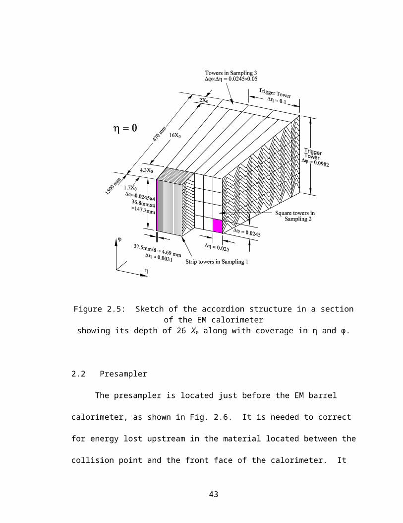
2.5 Sketch of the accordion structure in a section of the EM calorimeter showing its depth of 26Χ0 along with coverage in η and φ. 28

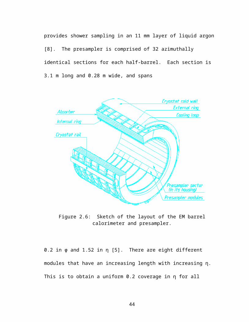
2.6 Sketch of the layout of the EM barrel calorimeter and presampler. 29

2.7 Presampler module with motherboard. 30

2.8 A back mother board on a module. 31

2.9 Sketch of a section of the EM calorimeter showing the summing boards and mother boards. 32

2.10 Sketch of the barrel showing the EM barrel calorimeter, the presampler, cabling, and the feedthroughs. 34

2.11 Side view of a feedthrough. 36

3.1 Sketch of a feedthrough flange showing fifteen rows and two

ix

columns. Each row of each column consists of 64 pins (128 for each full row).

40

3.2 Schematic of the complete read-out electronics chain. 41

3.3 Actual view of two adjoining feedthroughs with HV protection cards and scanner card inserted. 42

3.4 View of the PC, multimeter, and power source used during the test. 43

3.5 Ben Wakeland and myself (left) performing tests on the feedthroughs at the top of the M-wheel. 45

4.1 Graphs of the presampler data with variation respect to 2030 Ω vs. a) feedthrough position, b) position in η, c) position in φ, and d) the measured resistance distribution. 47

4.2 Graphs of the front data with variation respect to 3037 Ω vs. a) feedthrough position, b) position in η, c) position in φ, and d) the distribution of measured resistance. 49

4.3 Diagram illustrating the position of the protection circuits. 51

4.4 Graphs of the middle (η < 0.8) data with variation respect to 1061 Ω vs. a) feedthrough position, b) position in η, c) position in φ, and d) the distribution of the measured resistance. 52

4.5 Graphs of the middle (η > 0.8) data with variation respect to 735 Ω vs. a) feedthrough position, b) position in η, c) position in φ, and d) the distribution of the measured resistance. 53

4.6 Graphs of the back data with variation respect to 1061 Ω vs. a) feedthrough position, b) position in η, c) position in φ, and d) the distribution of the measured resistance. 55

4.7 The comparison of FT09-Back 0 (top) and FT00-Middle 1 (bottom) shows some correlation. 56

4.8 Data from two different scanner card tests on FT 23 – Mid 2. The plot shows a clear correlation in the different sections. 59

x

ACKNOWLEDGEMENTS

First and foremost, I would like to thank my advisor Ryszard Stroynowski. I have

been very fortunate to have his guidance, support, and patience during my graduate

studies at Southern Methodist University (SMU). The knowledge and expertise that he

has shared has helped me to better understand the aspects of particle physics research. I

am very thankful for being given the unique opportunity to work on the ATLAS detector

at CERN. I am also grateful to him for introducing me to wonderful Swiss cuisine, and

for a fantastic journey to the top of Aiguille du Midi to see Mont Blanc.

I am very grateful to Lydia Fayard, Christophe De la Taille, and Laurent Serin for

all of their help and support during the test of the M-Wheel. I want to especially thank

Ben Wakeland, who assisted in taking data. The data for this thesis would not have been

able to be fully collected without his “magic carpet” rides. I want to also thank Laurent

for the results of the data on which this thesis is based, and for all the help and insight he

has provided to help me better understand these results.

I feel a deep gratitude towards the SMU Physics Department. I would like to

thank the entire faculty for their support, and all of the knowledge they have shared

during my graduate studies. I am very grateful for being given the opportunity to study

in a department with so many talented faculty members. I can only hope that I will be

able to inspire my students as much as they have inspired me. I want to also thank

Shirley Melton and Carol Carroll helping me with all of my administrative problems.

xi

I am indebted to all of my fellow graduate students I have worked along side

during my time at SMU. I especially want to thank Liang Lu, Pavel Zarzhitsky, Eliana

Vianello and Yurii Maravin for their help with physics and other matters.

During my stay in Dallas, I thoroughly enjoyed the time I spent with my friends

Yurii, his wife Anya, and Eliana. Thank you all for the many great times we had out

having diner and watching movies. It was not the same after you left.

I am very grateful to my aunt and uncle, John and Brenda Knee, for everything

they have done for me while I have been in Dallas. Thank you so much. I am so

thankful that I was able to have family nearby. I only wish that we were able to spend

more time together.

I want to thank Benjamin Gross for his support and advice, and Zac Johnson for

all the great music he sent me. You guys are great friends.

Finally, I would like to thank my parents Randy and Lita for all the support,

encouragement, and love they have given me during my studies. I could not have asked

for better parents.

xii

CHAPTER I

INTRODUCTION

Particle physics is the study of the basic elements of matter and the forces that act

on them. The aim of particle physicists is to determine the fundamental laws that control

the make-up of matter and the physical universe. One of the many tools used to study

particle physics is the accelerator. It allows for the creation of the types of particle

collisions that we want to study. Experiments at particle accelerators collide sub-atomic

particles at very high energies, and they reveal details about particles and the conditions

that prevailed just after the Big Bang, which occurred over 15 billion years ago. The high

energy collisions between particles that physicists are interested in do occur naturally,

and are caused by cosmic rays. However, these events are unpredictable and the number

that can be observed is low. Therefore, we must create machines (accelerators) that can

make a large number of these events so that they can be better studied, and results can be

reproduced.

Accelerators work by accelerating charged particles using electric fields. There

are two basic types of accelerators: linear and circular. Linear colliders accelerate

particles in a straight line, while circular colliders accelerate particles in a circle. The

circular machines are more common due to economic factors. In addition to accelerating

the particles using an electric field, circular accelerators need to use a magnetic field to

bend their paths. In these machines, particles are accelerated in opposite directions until

1

they are brought together and forced to collide. One drawback to the circular machines is

loss of energy. Particles like to travel in a uniform direction. When they are forced to

change direction, such as in a circle by magnetic fields, they radiate energy in the form of

photons. This energy loss is known as Bremsstrahlung. This effect can be minimized by

increasing the radius of the ring, thereby reducing the curvature, but this increases the

cost of the accelerator.

At a collision point, a detector is needed to examine the particles that are

produced when accelerated particles collide. There are two basic types of detectors:

tracking detectors and calorimeters. Tracking detectors reveal the trajectories of

individual charged particles, and calorimeters measure the energies of both charged and

neutral particles. A modern detector is built using both. They are built with layers of

trackers and calorimeters to give as much information as possible about the particles

produced in each collision.

The main reason for studying particles is to enhance our knowledge, and

understanding, of matter, forces, and interactions. Theories and discoveries over the last

century by thousands of physicist have led to a remarkable picture of the fundamental

structure of matter, but not including gravitation. This picture is known as the Standard

Model of Fundamental Particles and Interactions, or Standard Model (SM) for short. The

SM has long (~20 yrs.) been a well tested physics theory that has been used to explain a

wide variety of phenomena. Many high precision experiments have been able to

repeatedly verify subtle effects that were predicted by the SM. The SM is a simple yet

comprehensive theory that explains all the hundreds of particles and their interactions

with 60 matter particles and 13 force carrying particles [1].

2

There are two families of matter particles: the quarks and the leptons. All of

these are point-like particles (they have no internal structure) and carry ½ integer spins.

The quark family consists of six quarks: bottom (b), charm (c), down (d), strange (s), top

(t), and up (u). The quarks are grouped in three generations because of similarities in

their properties of mass and charge, shown in Table 1.1: u/d, c/s, and t/b. Each of these

six quarks can have one of three different values (red, green, or blue) of a property known

as color, and for all of these 18 (6 × 3) quarks, there is an antiquark, making 36 total

quarks.

Table 1.1: Table of Quarks [1].

Flavor Name Spin Charge Mass (GeV) Generation

u up 1/2 2/3 0.0015 - 0.004 1

d down 1/2 −1/3 0.004 - 0.008 1

c charm 1/2 2/3 1.15 – 1.35 2

s strange 1/2 −1/3 0.080 – 0.130 2

t top 1/2 2/3 174.3 ± 5.1 3

b bottom 1/2 −1/3 4.1 – 4.4 3

There are also six leptons and six antileptons. Three of the leptons have mass and

charge: the electron (e-), muon (μ), and tau (τ). The other three have no charge and very

little mass: the electron-neutrino (νe), muon-neutrino (νμ), and tau-neutrino (ντ). Each of

the charged leptons associated with their respective neutrinos and quark pair make up the

3

first, second, and third generations of matter (i.e. e-, νe, and u/d make up the first

generation). Each generation is heavier than the one before it. Some of the properties of

the leptons are shown in Table 1.2.

Table 1.2: Some properties of leptons [1].

Name Spin Charge Mass (MeV) Generation

e- electron ½ -1 0.511 1

νe electron neutrino ½ 0 < 3 × 10-6 1

μ muon ½ -1 105.7 2

νμ muon neutrino ½ 0 < 0.19 2

τ tau ½ -1 1776.99 3

ντ tau neutrino ½ 0 < 18.2 3

Forces are transmitted between particles by the exchanging of the force carrying

particles which are called bosons. The SM includes three of the four known forces:

strong, weak and electromagnetic. Gravity, the weakest of the four, is not yet part of the

SM. They transfer small amounts of energy from one particle to another because they

have integer spin and follow Bose-Einstein statistics. These bosons are associated with a

specific force. The gluon (g; there are 8 colors of gluons) is associated with the strong

force, the photon (γ) is associated with the electromagnetic force, and the W± and Z

bosons are both associated with the weak force.

4

Early theories predicted that there was a symmetry between the photon, and the W

and Z bosons (Gauge Symmetry). These particles were predicted to all have zero rest

mass. However, observations have shown that in reality, this is not the case. In actuality,

the symmetry is “broken” or hidden [2]. The photon is massless (the gluon is also

massless), but the W and Z bosons were found to have significant mass. The W mass is

about 80 GeV, and the Z mass is about 91 GeV [1]. This large mass of the carrier bosons

restricts the weak force to a short range, unlike the electromagnetic force whose range is

infinite because photons have no mass. A complete internal symmetry is found in the

mathematical description of weak and electromagnetic interactions, except for the effects

of the masses. This physical phenomenon is known as electroweak symmetry breaking,

and the mechanism behind it has yet to be discovered.

The SM predicts that a new particle, the Higgs boson, interacts with both matter

and force carrying particles to give mass to all particles (Higgs mechanism) [2].

According to the theory, the mass is related to the strength of the interaction with the

Higgs boson: the stronger the interaction, the greater the mass. The Higgs boson is the

only undiscovered particle predicted by the SM.

The theory of supersymmetry (SUSY) is a possible extension of the Standard

Model. It differs from all other symmetries because it relates two types of fundamentally

different elementary particles: fermions (spin = 1/2, 3/2, 5/2, etc.) and bosons (spin = 0,

1, 2, etc.) [2]. According to the SUSY theory, every particle has a supersymmetric

partner that differs in spin by 1/2. So, to clarify, fermions have bosonic supersymmetric

partners, and bosons have fermionic supersymmetric partners. The strength of

interactions of these supersymmetric particles is identical to the corresponding ‘ordinary’

5

particles. These SUSY particles are named in the following way: the bosonic

supersymmetric partners of the fermions have the prefix ‘s-’ added to the fermion name,

and the fermionic supersymmetric partners of the bosons have the suffix ‘-ino’ added to

the boson name. So, for example, a spin 1/2 electron (e) has a spin 0 SUSY particle

called a selectron (e), and a spin 1 photon (γ) has a spin 1/2 SUSY particle called a

photino (γ). SUSY particles are denoted by a tilde (~) above the partner’s symbol.

There are a few different models for SUSY, but the general idea is that there is a

broken symmetry in supersymmetry. This comes from the experimental evidence, or lack

of evidence in this case. If SUSY was without broken symmetry, we would see sleptons

with the same masses as leptons, squarks with the same masses as quarks, and so on [2].

No such particles have been observed, and so if SUSY is to be a true symmetry of

particle physics, it must be broken. This breaking of symmetry allows for the SUSY

particles to be much heavier than their partners [2]. This could explain why SUSY

particles have not yet been seen because we haven’t been able to reach the energies

required to create these heavy particles.

Heavy SUSY particles are thought to decay like the ‘ordinary’ particles

that they resemble (not like their partners). Starting with the primary SUSY partner

(X), X will decay all the way down to the lightest supersymmetric particle (LSP) plus

some other normal particles. The observation of this LSP is the important starting point

for ATLAS to verify whether SUSY exists or not.

Experiments to date have not been able to show that these theories are correct.

Current particle accelerators have not had the ability to reach a high enough energy to be

able to detect a Higgs boson or SUSY particles. However, this may soon change. There

6

is a new collider being built that will go beyond the expected range needed (according to

the theories). It is called the Large Hadron Collider (LHC), and it is expected to go

online in 2007. One of two experimental detectors that will focus on trying to find the

Higgs boson is called ATLAS (A Toroidal LHC ApparatuS) [3].

In this chapter, after a brief introduction to the ATLAS detector and the physics

goals of the experiment, I will give an introduction to the testing of the electronics chain

of the electromagnetic barrel calorimeter.

1.1 LHC and ATLAS

The Large Hadron Collider (LHC) is a large particle accelerator project at the

European Laboratory for Particle Physics (CERN) located in Geneva, Switzerland. The

LHC is designed to collide bunches of protons every 25 ns. These beam crossings will

occur when two bunches of protons are accelerated in opposite directions around a 27 km

ring (circumference). Each bunch, with an energy of 7 TeV, is then brought together into

a collision. The proton-proton collisions will have a center of mass energy of 14 TeV.

At the desired luminosity (1034 cm-2s-1), there will be a total of ~23 interactions per beam

crossing every 25 ns apart. The main goal of the LHC is to maximize the discovery

potential for new physics such as the Higgs boson and supersymmetric particles, while

still being able to measure known objects such as heavy quarks and gauge bosons with a

high degree of accuracy.

7

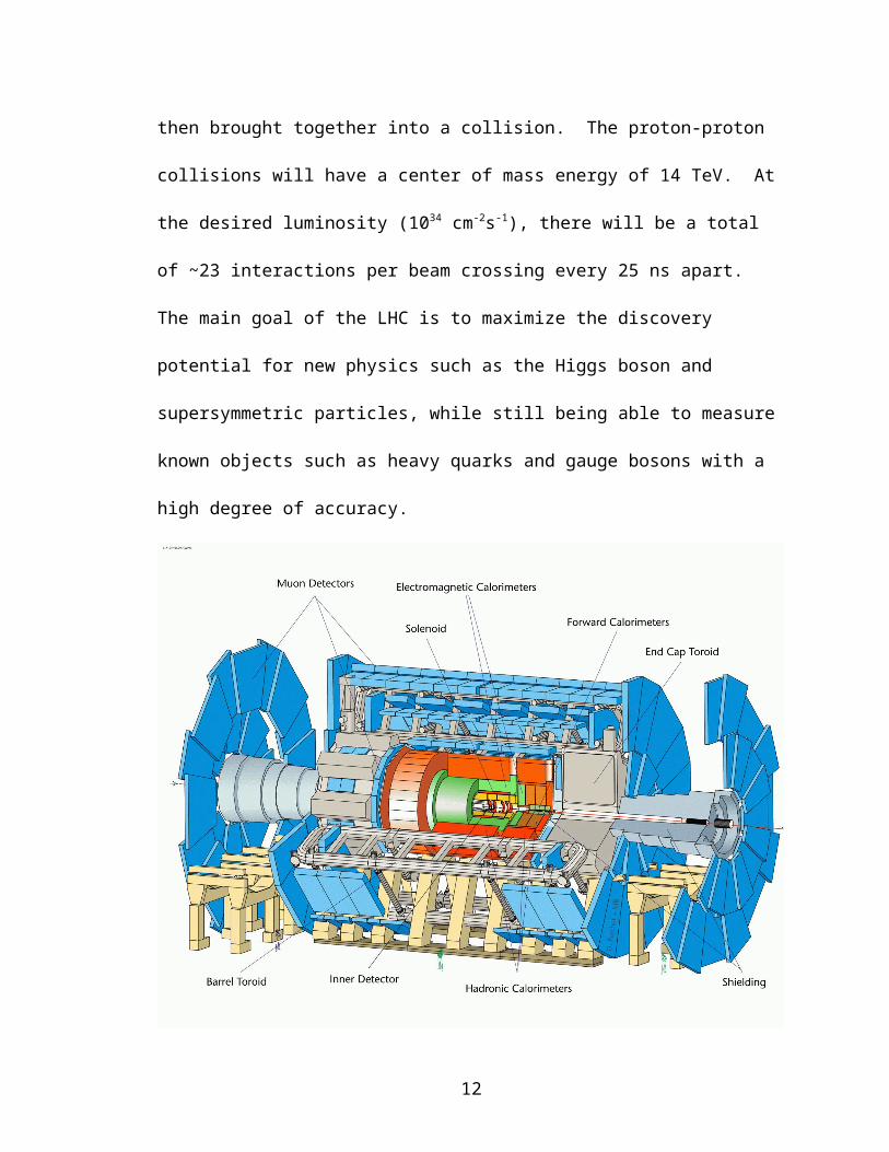
Figure 1.1: Three dimensional view of the ATLAS detector.

The ATLAS detector is one of the experiments at the LHC. This experiment will

study these proton-proton collisions at energies seven times larger than the highest

available to date. The group that is working on ATLAS is comprised of nearly 2000

collaborators from over 150 institutions from all over the world [3]. It consists of five

major components: the inner detector, the electromagnetic calorimeters, the hadronic

calorimeters, the muon spectrometer, and the magnet system. The ATLAS components

can be seen in Fig. 1.1. The reason that detectors are divided into different components is

that each component measures a special set of particle properties. The different types of

particles react in unique ways, so it is important to have specialized detector parts. These

8

Figure 1.2: Interaction of various particles with the different components of a detector.

components are stacked so that all particles will go through the different layers in a

preferable order. A particle will be noticeable when it either interacts with the detector in

a measurable fashion, or decays into detectable particles. An illustration of how particles

interact with the different parts of the detector can be seen in Fig. 1.2.

1.1.1 Inner Detector

The Inner Detector is the first detector the particles will interact with as they

move out from the collision point [3]. It is comprised of a set of tracking devices to track

charged particles from the collision point to the electromagnetic calorimeter, and

determine these trajectories with a high degree of accuracy. The Inner Detector is also

designed to take momentum and vertex measurements, and identify electrons. It

accomplishes all of this by being constructed of three major subdetector parts: the Pixel

detector, SemiConductor Tracker, and Transition Radiation Tracker. The Pixel detector

9

and the SemiConductor Tracker are responsible for taking the momentum and vertex

measurements, and the Transition Radiation Tracker is responsible for finding the

trajectories of the particles.

The Pixel detector is designed to take three high-precision measurements as close

to the collision point as possible. It accomplishes this with three layers of pixels arranged

in a barrel shape with radii of ~ 4 cm, 10 cm, and 13 cm. There are also five disks of

pixels located on each side of the pixel barrel. One of its primary functions is to find

short lived particles (i.e. B hadrons and tau leptons) by detecting secondary vertices away

from the collision point.

The SemiConductor Tracker is located just after the pixel detector. It is

composed of highly segmented sensing devices made from strips of silicon. As the

charged particles pass through the silicon, they deposit a measurable amount of energy.

The SemiConductor Tracker is designed to take eight precision measurements. Its design

is similar to the pixel detector, as it also has a barrel and end-cap disks, but the

SemiConductor Tracker is comprised of eight layers.

The outer most part of the Inner Detector is the Transition Radiation Tracker. It is

designed to take an average of 36 precision measurements through ~36 layers of straw

tube detectors. In addition to the tracking information, its main purpose is to identify

electrons by detecting transition radiation photons. To accomplish this, xenon gas is used

between the straws. When the electrons pass through the xenon gas, they give off

photons.

10

1.1.2 Electromagnetic Calorimeter

The ATLAS electromagnetic (EM) calorimeter is a lead-liquid argon

detector with accordion shaped geometry [3]. It is comprised of three main parts: the

barrel, and two end-caps. They are shown in Fig. 1.3. The main focus for ATLAS is to

search for the Higgs boson (H). As stated above, the Higgs boson is theorized to be the

key to how particles acquire mass. A decay of the Higgs into a pair of photons is a

favored channel because of its clear signature [6]. Therefore, the EM calorimeter is a

crucial part of ATLAS. A detailed description of the EM calorimeter parts will be

discussed in Chapter II.

The EM calorimeter is designed to measure the total energy of electrons,

positrons (e+), and photons. Essentially the EM calorimeter will be measuring the energy

deposited by electromagnetic showers. Electromagnetic showers are cascading events

that are caused when electrons or positrons interact with matter in the calorimeter causing

them to radiate photons. The photons then convert into e+ e- pairs, which then also

interact and radiate photons that will then also decay into more e+ e- pairs. This cascade

will continue until the average energy of the particles in the shower drops below the

critical energy for the electron pair conversion.

There are two different types of material that can be used for the active material

layer: gas or liquid. The use of liquids has some advantage over gasses when used as

detectors for charged particles. The density of liquids is almost one thousand times

greater than that of gasses [4]. Also, the energy absorbed per unit thickness of the layer

is much larger in liquids by about the same factor, and the number of electrons formed in

the shower process is much greater as well. The only drawback is that liquids are harder

11

to purify. To minimize this problem, noble gases (He, Ne, Ar, Kr, Xe, Rn) are chosen

because their chemically inert properties make it relatively easy to maintain their purity

to a standard that is required in the detector. They are also chosen because they are

inexpensive, readily available, and can be easily transformed into their liquid state by

being cooled below their boiling point. Impurities such as oxygen (O2) will readily

absorb electrons, and thus negatively affect the measurements by reducing the shower.

Liquid argon (LAr) has been chosen to be used in ATLAS, with an impurity level below

2 parts per million (ppm) [5]. The boiling point for LAr is 87.45 K, which is about

-303° F.

The extremely cold temperature that the LAr needs requires special cooling, and

isolation from warm temperatures. Therefore, the EM calorimeter is housed in what is

known as the cryostat. The cryostat acts like a refrigerator, keeping the inside cold and

the warm air out.

1.1.3 Hadronic Calorimeter

The hadronic calorimeter is comprised of two sections located in the outer areas

of the same barrel and end-caps as the EM calorimeter [3]. Its primary function is to

measure the total energy of hadronic particles by measuring the hadronic showers. A

hadronic shower starts when a hadron interacts with the calorimeter material and the

interaction creates secondary hadrons. These secondary hadrons then interact with the

calorimeter material and form tertiary hadrons. This process will continue until they are

stopped by ionization energy loss or they are absorbed. An important aspect in the design

of the hadronic calorimeter is its thickness. It is important for the hadronic calorimeter to

12

contain as much of the hadronic showers as possible so that it minimizes the carry over

into muon system [4]. The hadronic calorimeter is also used to measure missing

transverse energy, which is important for many physics signatures including searches for

supersymmetric particles.

Figure 1.3: EM and hadronic calorimeters.

13

There are two different parts of the hadronic calorimeter, and they are constructed of

different material. The first part is constructed with iron as the absorber material and

scintillating tiles as the active material for sampling [3]. This design has parts in the

outer portion of the barrel and the end-caps. The second part is located only in the end

caps. This part uses copper as the absorber material and electrodes for the sampling.

Both parts are oriented radially around the beam axis. This design can be seen in

Fig. 1.3.

1.1.4 Muon system

The purpose of the muon system is to detect muons, one of only two types of

particles to penetrate all material of the detector (the other are neutrinos). It is a three

layer system of chambers in a toroidal magnetic field that provides precise measurements

of the momentum of muons [3]. This information can be combined with information from

the inner tracker to further improve the momentum measurement. The muon system is

composed of two main parts: the muon toroidal magnets and the muon detector.

The muon toroidal magnet system has two parts: the barrel toroids and two end-

cap toroids. They both can be seen in Fig. 1.1. The barrel toroid consists of eight

toroidal magnets that generate a toroidal magnetic field that runs through the center of the

toroids, and which surrounds the inner portion of the detector. The end-cap toroids are

located in the end-cap region just at the end of the barrel toroids. This set up provides a

radial overlap and optimizes the bending power is this area. The magnetic field is

important because it will bend the path of the muons. This magnetic deflection is

important for the momentum measurements needed to be taken in the muon system. The

14

radius of curvature along with its direction will determine a particles momentum and the

sign of its charge. Having the magnetic system also minimizes the amount of material

through which the muons have to travel, which reduces multiple scattering and therefore

improves the muon momentum measurement.

There are two parts in the muon detector system. They are designed to take three

measurements of particles originating from the interaction point. The first part is

arranged around the barrel, and consists of three concentric cylinders. The second part

consists of four concentric disks located on each side of the interaction point at the ends

of the detector.

1.1.5 Magnet system

The magnet system in ATLAS is comprised of two main parts: the toroidal

magnets discussed above, and the solenoid magnet. As stated above, magnets play a key

role in providing a magnetic field to bend charged particles so that important physics

measurements can be made. Since the toroids have already been discussed, this section

will only focus on the solenoid magnet.

The solenoid magnet (see Fig. 1.1) provides a magnetic field for the inner

detector. The solenoid is a large coil of wire wound cylindrically to generate a straight

uniform magnetic field inside the coil [3]. It provides the magnetic field to the inner

detector by being constructed on its outer radius. The trajectory of charged particles

curve in the magnetic field (B), and the radius of curvature R is proportional to the

particles momentum (p) by the expression p 0.3 B R, where B is in teslas and R is in

meters [1].

15

1.2 Physics goals of the ATLAS experiment

Most of us are familiar with forces that are associated with electric, magnetic, and

gravitational fields. It is theorized that there is a new field that has yet to be discovered

that is responsible for giving the particles mass. It is proposed that this field, called a

Higgs field, permeates all of space, and that when particles interact with this field, they

acquire mass. It is also proposed that the strength of the interaction is proportional to the

mass that a particle will acquire. A particle that interacts strongly with the Higgs field

will be heavy, while a particle that interacts weakly will be light. According to the

theory, particles interacting with the Higgs field will actually be interacting with a new

particle that is associated with this field, called the Higgs boson. The discovery of the

Higgs boson at ATLAS would be one of the greatest scientific discoveries to date.

Another important question that ATLAS hopes to answer is if the electroweak and

the strong forces can be unified. In the 1967, there was a major breakthrough in particle

physics. This was the development of a unified description of the electromagnetic and

weak forces (electroweak) by Steven Weinberg, a physicist from Harvard [2]. Physicists

are now attempting to broaden this unification into a “grand unification” by including the

strong force.

Experiments have shown that the effects of the strong force become weaker as the

interaction energies increase. This suggests that at very high energies, the strengths of

the electromagnetic, weak and strong forces are the same. The forces would basically be

indistinguishable. Unfortunately, the energies involved are a trillion times greater than

particle accelerators can reach. However, there is some good news. The grand unified

theories have some consequences at lower energies; therefore, they can still be tested.

16

Supersymmetry (SUSY; see above) is one type of grand unified theory (GUT). If

SUSY is right, then supersymmetric particles should be found by ATLAS.

Measurements by astronomers have lead to a conclusion that 90 % or more of the

Universe does not emit electromagnetic radiation, and therefore is not visible. Scientists

call this invisible material dark matter. Very little is known about the nature of dark

matter and its role in the universe. It is probable that dark matter is made of several

different components, including neutrinos and supersymmetric particles. ATLAS hopes

to answer some questions about dark matter by finding some of these particles.

Another fundamental question that ATLAS hopes to answer is why there are three

generations of matter (see above). This puzzle is linked to one of the great mysteries of

the universe. For a long time scientists have been trying to figure what happened to all

the antimatter. Experiments in particle physics have shown that matter and antimatter are

always created in equal quantities. This indicates that this equal creation should also

have happened at the Big Bang. We also know that when matter and antimatter collide,

they annihilate. However, there is a lot of matter that remains in the universe, and no

antimatter. Therefore it is puzzling as to why the antimatter did not completely annihilate

all the matter.

The fact that there is a lot of matter left in the universe seems to point to some

small but significant asymmetry between matter and antimatter. This asymmetry could

come from an effect that is called CP-violation. Thus far, CP-violation has been seen

affecting particles that contain the strange quark from the 2nd generation. The LHC

should easily produce particles containing the heavier bottom quark from the 3rd

17

generation. If the theory is correct, ATLAS should be able to detect the symmetry

breaking CP-violation in these particles as well.

1.3 Electronics chain in the EM Calorimeter

Many of the important physics processes at the LHC involve particles that decay

into electrons or photons. The detection and reconstruction of these events depend on

very good electromagnetic calorimetry. Therefore, it is very important the signals from

the EM calorimeter are able to be read out accurately. This requires many important tests

to ensure that the electronics are well understood and working properly. One such test is

the testing of the complete electronics chain in a warm environment, before the liquid

argon is added. This test will be performed in four different parts because of the separate

EM calorimeter parts (two half-barrels, and two end-caps). One of these tests took place

during July 2003 at CERN (bldg. 180). It was performed on one of the half-barrels. This

thesis will focus on that test, and a detailed description will be given in Chapter III.

The complete electronics chain in the EM barrel calorimeter is fairly complex,

and its individual components will be discussed in detail in Chapter II. Essentially, the

signal is read out from electrodes in the accordion section. Multiple electrodes are added

together to form one channel in summing boards. From here, the signals from the

channels are sent through mother boards, which ensure the signal routing. The signals

are then routed out of the module by 64 coaxial cables that are attached to the mother

boards. The total cable route is comprised of two sets of cables in parallel separated by a

patch panel. The signals are then routed out of the EM calorimeter by way of

feedthroughs, special chambers that are required to separate the cold environment of the

18

cryostat from the warm environment of the electronics required to analyze the signals.

The feedthroughs are comprised of a vacuum chamber with cables that are attached to a

pin interface at both ends.

A detailed description of the electromagnetic barrel calorimeter will be discussed

in Chapter II. Then in Chapter III, I will focus entirely on the set-up and procedure of the

test that was performed on the complete electronics chain of one of the half-barrels in the

electromagnetic barrel calorimeter. Finally, the results and conclusions of this test will

be given in Chapter IV.

19

CHAPTER II

ELECTROMAGNETIC CALORIMETER

An electromagnetic (EM) calorimeter is a device that measures the energy of

particles that interact primarily through the EM force. Such particles are electrons,

positrons, and photons. When electromagnetically interacting particles pass through

matter, they deposit energy by a number of processes. At the energies that the LHC will

operate, the dominant interaction will be e+e- pair production (γ e+e-) and

bremsstrahlung (e e γ) [7]. The e+e- pair is created through the interaction of the

photon with the electric field of a nucleus in the material. Alternating sequences of these

two types of interactions leads to a cascade of electrons, positrons, and photons. This

cascade is known as an EM shower. A simplified sketch of the development of an EM

Figure 2.1: Simplified development of an EM shower.

20

shower is shown in Fig. 2.1. Bremsstrahlung is the radiating of a photon by an energetic

electron or positron that passes through matter and is scattered by the electric fields of

nuclei in the material.

The initial particles will radiate bremsstrahlung photons and lose energy due to

ionization and scattering until they are stopped in the medium. This will occur when the

average energy of the particles in the shower drops below the critical energy (Ec) that is

characteristic of the material. The critical energy is defined to be the point at which the

energy loss of electrons by ionization equals the energy loss by bremsstrahlung. It is

given by an approximate formula Ec ≈ 800 (MeV)/ (Z +1.2) [7], where Z is the atomic

number of the material.

The characteristics of an EM shower are influenced by the electron density of the

material. This density is proportional to Z. The longitudinal and transverse dimensions

of an EM shower are described by two material independent quantities. The radiation

length (Χ0) characterizes the longitudinal shower dimension. It is defined to be the

average distance over which an energetic (> 1 GeV) electron will radiate 63 % (1 -1/e) of

its energy by bremsstrahlung only [7]. The transverse spread of an EM shower is caused

by three things: multiple scattering of electrons away from the shower axis, the angle

between the particles in e+e- pairs, and bremsstrahlung photons that are emitted away

from the shower axis. The unit that describes the width of the spread is the Moliere

radius (Rm). It is defined by Rm = EsΧ0/Ec, where Es ≈ 21 MeV [7]. Approximately 95 %

of a shower’s energy will be contained within an infinite cylinder of radius 2 Rm.

An equivalent distance for the interaction of photons is called the mean free

path (Χγ). The mean free path is the distance after which the number of photons of

21

identical energy has decreased by 1/e through pair creation. This is given by the formula:

Χγ = 9/7 Χ0. The two processes, bremsstrahlung and pair creation, have a comparable

importance in that the function of depth is almost equal. However, the fraction of the

cascade energy carried by the photons will increase as the depth of the shower increases.

A simple model of an EM shower can be obtained by considering the total

number N of particles present in a shower after n radiation lengths of material. This is

given by N ≈ 2n. The average energy of each particle is E (n) ≈ E0/2n, where E0 is the

energy of the electron or photon which initiates the shower. When the average particle

energy drops below Ec, fewer particles are produced than are absorbed by the medium.

The maximum number of particles in a shower is therefore given by Nmax ≈ E0/Ec. Since

we can assume that the shower will end when the particle energy drops below Ec, we can

then find the shower’s penetration depth by E (nmax) = E0/2nmax = Ec. Solving for nmax we

then have

nmax = ln (E0/Ec) / ln 2.

The penetration depth is therefore related to the log of the particle energy. Typically

about 25 Χ0 are required to contain 95 % of the energy of a 100 GeV EM shower. Since

the longitudinal shower energy containment is scaled in this way, it means that the

overall size of the calorimeter can be kept rather compact.

Each charged particle in an EM shower will lose energy through ionization of the

medium. This produces a large number of electrons that can be used to produce a

measurable signal. The measurable signal produced in a calorimeter can take a number

of forms depending on the type of calorimeter. One of these forms, which is utilized in

22

the ATLAS EM calorimeter, is an electric current produced by the drift of ionization

charge in the layers of active material in the calorimeter.

The ATLAS EM calorimeter utilizes liquid argon (LAr) as its active medium. A

simplified description of a cell in a LAr calorimeter consists of a liquid argon gap,

bounded on two sides by absorber layers. A read-out electrode layer is placed in the

middle of the gap and a high voltage is applied to the electrode relative to the absorbers

in order to produce an electric field in the gap. An ionizing particle crossing the LAr gap

in a direction perpendicular to the absorber plates creates a line of electrons that drift

toward the read-out electrodes by the influence of the electric field. These charges are

then collected at the read-out electrodes, producing a current. This current pulse is then

amplified and combined with the signals from other cells to reconstruct the energy of the

incident particle. A more thorough description will be discussed in detail in section 2.1.

As stated in the Introduction, the ATLAS EM calorimeter has three sections: two

end-cap EM calorimeters and an EM barrel calorimeter composed of two half-barrel

calorimeter sections. Since this thesis focuses on the test that was preformed on the

complete electronics chain of one of the EM half-barrel calorimeters, the detailed

description of the ATLAS EM calorimeter here will be limited to just the half-barrel

section, and it will focus on the parts of the calorimeter that directly relate to the test.

I will first give a detailed description of the design of the EM barrel calorimeter in

sec. 2.1, and in sec. 2.2 the design and purpose of the presampler will be discussed. Then

in sections 2.3 and 2.4, I will give a description of the important electronics and the

feedthroughs that are important to the reading out of the signals from the calorimeter.

23

Figure 2.2: Simulation of an electromagnetic shower in the barrel EM calorimeter.

2.1 Barrel Calorimeter

The EM barrel calorimeter is a lead Liquid Argon (LAr) detector with accordion

shaped geometry. A view of this accordion geometry can be seen in Fig. 2.2. This

accordion shaped geometry provides complete coverage in the φ direction (the φ

direction is the radial direction around the beam axis) without any gaps. The EM barrel

calorimeter is comprised of two half-barrels of equal design. Each half-barrel is made of

1024 accordion shaped absorbers alternated with read-out electrodes [8]. This setup has

an advantage in that the read-out electronics can be placed on the inner and outer radius

of the electrodes instead of having them run in the radial direction. This reduces the

inductance in the on-detector electronics, thereby improving the pulse shape and timing

for the read-out electronics. Even though there are no gaps, each half-barrel is divided

into 16 modules.

24

The half-barrels are separate from each other, and each is connected to their

respective ends of the cryostat. The length of each half-barrel is 3.2 m, and they both

have an inner diameter of 2.8 m, and an outer diameter of 4 m. Each half-barrel is

designed to cover the psuedorapidity from |η| = 0 to |η| = 1.475, illustrated in Fig. 2.3.

The structure of the absorbers is comprised of three parts. The main part of the

absorber is made of lead sheets of different thickness. The thickness varies from

1.53 mm for η < 0.8 to 1.13 mm for η > 0.8. This variation in thickness is important

because it decreases the sampling frequency at high η. The lead sheets are glued between

Figure 2.3: Longitudinal slice of the EM calorimeter showing that the barrel section covers |η| = 1.475.

25

two 0.2 mm thick stainless steel sheets. The lead and steel sheets are glued together by

using resin soaked fiberglass fabric. The fiberglass compensates for the variation in

thickness to give the absorbers a nominal thickness of 2.2 mm. The purpose of the steel

sheets is to provide mechanical strength for the absorbers.

The read-out electrodes are composed of three layers of conductive cooper with

insulating kapton polyimide sheets separating them. The structure of the read-out

electrodes is shown in Fig. 2.4. The inner layer is used to read out the signal, while the

outer layers are used to create an electric field by keeping a high voltage potential. The

electrodes have a total thickness of 275 μm [5].

The accordion shape of the absorbers is designed so that the folding angles are

decreasing with increasing radius. This insures that there is an approximately constant

gap of 4.5 mm between to adjacent sides. The accordion structure is shown in Fig. 2.5.

The electrodes are placed in the center of these gaps, giving them a 2.1mm liquid argon

gap on either side. The EM barrel calorimeter is divided into three sections by depth:

front, middle, and back.

26

Figure 2.4: Structure of the read-out electrodes.

27

Figure 2.5: Sketch of the accordion structure in a section of the EM calorimetershowing its depth of 26 Χ0 along with coverage in η and φ.

2.2 Presampler

The presampler is located just before the EM barrel calorimeter, as shown in Fig.

2.6. It is needed to correct for energy lost upstream in the material located between the

collision point and the front face of the calorimeter. It provides shower sampling in an

11 mm layer of liquid argon [8]. The presampler is comprised of 32 azimuthally identical

sections for each half-barrel. Each section is 3.1 m long and 0.28 m wide, and spans

28

Figure 2.6: Sketch of the layout of the EM barrel calorimeter and presampler.

0.2 in φ and 1.52 in η [5]. There are eight different modules that have an increasing

length with increasing η. This is to obtain a uniform 0.2 coverage in η for all modules

except the module located at the end of the barrel which only covers 0.12 in η.

The modules are composed of alternating cathode and anode electrodes that are

glued between glass-epoxy insulation (FR4) layers. The cathodes are double-sided

printed circuit boards, and the anodes are made of three conductive layers that are

separated by FR4 layers. The cathodes are 270 μm thick and the anodes are 327.5 μm

thick [5]. The outer layers of the anodes are kept at a high voltage of 2 kV, while the

inner layer is used to read out the signal. The spacing of the electrodes varies between

1.9 and 2.0 mm for the different sized modules.

29

Each module has a mother board attached to it, as seen in Fig. 2.7. The mother

boards are matched in size to the modules, thus there are eight different sized mother

boards. The mother boards are used to collect the readout signals, and to inject the

calibration pulses.

Figure 2.7: Presampler module with motherboard.

2.3 Electronics

The signals from the front section of the EM barrel calorimeter are read out from

the inner side of the electrodes, while the middle and back sections are read out from the

outer side of the electrodes [8]. The calorimeter signals from adjacent read-out electrodes

are summed together from the φ direction by summing boards. In the back and middle

30

Figure 2.8: A back mother board on a module.

sections, four adjacent electrodes are summed together, and in the front, 16 adjacent

electrodes are summed together. Each of these sums is considered one read-out channel.

The signal is then passed on to mother boards. Each mother board in the front

section provides read-out for 16 summing boards, while the mother boards for the back

and middle sections provide read-out for 4 summing boards. A mother board from the

back section can be seen in Fig. 2.8. The size of the mother boards increases with

rapidity because they read-out a constant rapidity (η) region. There are 7 different types

31

Figure 2.9: Sketch of a section of the EM calorimeter showing the summing boards and mother boards.

of mother boards for the back section, and 8 different types for the front section. For

each barrel module, there are a total of 14 back mother boards and 16 front mother

boards.

The mother boards are connected to the summing boards by pins mounted on 2

thin PC-boards. The position of the mother boards and summing boards can be seen in

Fig. 2.9. There are over 100 pin connections between each mother board and summing

board. One of the two PC-boards houses a voltage suppressor to protect against any

accidental discharge that could damage the calibration resistors on the mother boards. It

is a low capacitance transient voltage suppressor that turns on at 6 V. There is also a

32

15 μm thick G10 board that electrically separates the mother board and summing board

(see Fig. 2.8).

The mother boards route the signals to the read-out cables, shown in Fig. 2.8.

This is done through a “low profile” connector which minimizes cross-talk between the

read-out channels. Two different types of cables are used for this because of the different

impedance needed in each section of the EM barrel calorimeter. A cable of 50 Ω is used

for the front section, and a cable of 25 Ω is used for the middle and back sections. These

cables are mini coaxial cables. They are bundled together in groups of 64. These bundles

are called harnesses. Two harnesses complete the connection from the mother boards to

the feedthroughs. The first harnesses go from the mother boards to patch panels, and the

second harnesses go from the patch panels to the feedthroughs.

2.4 Feedthroughs

Each of the two half-barrels has their signals brought out by feedthroughs located

at both ends of the cryostat. There are 32 feedthroughs located radially around each end

of the barrel cryostat, for a total of 64. These feedthroughs, as seen in Fig. 2.10, are

responsible for bringing the 122,880 signal, monitoring, and calibration lines into a warm

environment from the cold liquid argon environment [8]. Each feedthrough provides

connections for 1920 signal and calibration lines. The feedthroughs are an insulating

vacuum that minimizes heat contamination of the liquid argon area.

33

Figure 2.10: Sketch of the barrel showing the EM barrel calorimeter, the presampler, cabling, and the feedthroughs.

The feedthroughs are mainly comprised of a cold flange and a warm flange, and a

flexible stainless steel bellows. A diagram of the feedthroughs can be seen in Fig. 2.11.

34

The purpose of the flexible bellows is to allow for the near 1.5 cm movement of the two

flanges during the cool down from room temperature to the temperature of the liquid

argon. All three pieces are welded together. The cold flange is attached to the cryostat,

and the warm flange is connected to the front end crate electronics.

Both flanges have the same electrical connection design. They consist of two

7-row and two 8-row pin carriers. Each pin carrier consists of 64 pins in dual-inline rows

separated by a row of pins that are grounded. The pins are gold-plated to ensure

excellent, low resistivity contacts, and are sealed in glass for insulation.

The connections that transfer the signals from the cold flange to the warm flange

are comprised of flat cables that are approximately 25 cm long. The impedance of 35 Ω

was chosen so that they could use the same cables for both the 25 Ω and 50 Ω cables

from the mother boards.

At the warm flange, the cables are connected to the base-plane of the front-end

crate. This is essentially a group of pins, whose function is the transmission of the

signals to the read-out electronics. The tests performed in July 2003 utilized these base-

plane pins to inject a test signal into the complete read-out electronics chain and measure

the reflected pulse.

35

Figure 2.11: Side view of a feedthrough.

36

CHAPTER III

TEST OF COMPLETE READ-OUT ELECTRONICS CHAIN

The test of the complete read-out electronics chain is one of the important tests

that need to be preformed on the EM calorimeter. The motivation for ensuring that all

~220,000 channels work properly comes from all of the physics processes that ALTAS

hopes to look for, especially the search for supersymmetric particles.

The LSP (discussed in Chapter I) is expected to be a neutral particle that will not

interact in the detector, and thus escapes. However, its signal will show up as missing

transverse energy (ETmiss) in the event. Therefore, ET

miss is an important measurement.

Missing transverse energy (ETmiss) is a measurement that comes from summing all

the signals of the detector. We are able to perfectly reconstruct the energy deposited in

the detector, and if there is a supersymmetric particle that escapes detection, it will carry

out some transverse energy and in the overall balance there will be missing transverse

energy. If the number of observed events with a large amount of ETmiss is larger than

expected from normal statistical principles, then this is a signal of some new physics,

very likely a supersymmetry.

It should be easy to see that we do not want to see an artificial high ETmiss

generated by detector malfunction or mis-calibration. Therefore, it is important to

minimize fake ETmiss events so that genuine ET

miss events can be observed. One possible

way to get a fake ETmiss event is by having holes in the EM calorimeter. So, it is important

37

to ensure that the EM calorimeter is working properly. Therefore, it must be tested

before it is installed in the ATLAS detector.

There are two other important aspects of the test performed for this thesis. The

first is that the EM barrel calorimeter is warm, and only filled with air, i.e. the liquid

argon has not yet been inserted. It is important for us to test the calorimeter in its warm

state because once the liquid argon is added it would be very time consuming to have to

fix something if a problem was found. If a repair was needed, it would require warming

up the calorimeter and then removing the liquid argon that will be at around 300° F

below room temperature. This is a process that would take over four months to complete.

The other important aspect is that the test was preformed before the EM barrel

calorimeter is assembled together with the rest of the detector. If a problem is found after

the whole detector is assembled, it would take many more months (~12) to take the

detector apart to get to the EM barrel calorimeter.

The test was conducted on the complete read-out electronics chain of the M-wheel

of the barrel EM calorimeter (the other end is designated as the P-wheel) during July

2003 in Building 180 at CERN. In Chapter II, all of the individual sections of the

complete electronic chain are described in detail. In the remainder of this chapter, I will

describe the set-up and procedure for the test. A photograph taken during the test can be

seen in Fig. 3.5.

38

3.1 Set-up and Equipment

The test of the complete read-out electronics of the M-wheel was conducted using

a plug-in dedicated scanner card at the base-planes of the connectors in the feedthroughs.

The connectors are arranged in two columns and 15 rows (see Fig. 3.1); each row is

comprised of a connector from both columns, and contains 128 channels in total. Each

connector consists of 64 pins, and each channel corresponds to a pin in the feedthrough

flange. All 128 channels (A and B columns together) measured, are chosen one after the

other by the scanner. The scanner software was commanded through a GPIB.

A schematic of the complete read-out electronics chain can be seen in Fig. 3.2. A

power supply, set at approximately + 8 V, connected to the scanner card was used to send

a pulse through the complete read-out electronics chain. The pulse bounced back at the

end of the chain and the resistance of the entire chain was then measured by a Keithlay

multimeter. The measurement of the resistance was then recorded and stored on a laptop

PC. The actual power supply, multimeter, and laptop PC used in the test can be seen in

Fig. 3.4.

39

Figure 3.1: Sketch of a feedthrough flange showing fifteen rows and two columns. Each row of each column consists of 64 pins (128 for each full row).

3.2 Operational Procedure

The resistance measurements in each of the feedthroughs followed the same

procedure. The first step was to remove the metal box that covered two adjoining

feedthroughs. The metal box was used to protect the feedthrough connections until the

40

Figure 3.2: Schematic of the complete read-out electronics chain.

front end crate electronics are installed. The next step was to remove the 50 Ω high-

voltage (HV) protection cards that were plugged into each of the connectors. These HV

protection cards were used to protect against damage from high voltage, and they can be

seen in Fig. 3.3. After these cards were removed, the next step was to conduct the

measurements in both of the adjoining feedthroughs.

The measurement procedure consisted of four steps. The first step was to insert

the scanner card into the connector slot that was to be tested. The second step was to

then make sure that the multimeter and power supply were both turned on, and at the

correct settings. The next step was to initiate the computer program that started the test

and recorded the resistance measurement on every channel. The final step was to save

the data file for each set. It can be seen in Fig. 3.1 that every feedthrough has a

component of the each of the calorimeter sections: front, middle, back, and presampler.

The final steps of the entire test were to plug the HV protection cards back into

the connectors, and then reconnect the metal box to protect the two feedthroughs.

41

Figure 3.3: Actual view of two adjoining feedthroughs with HV protection cards and scanner card inserted.

42

Figure 3.4: View of the PC, multimeter, and power source used during the test.

3.3 Measurement Expectations

It has been established by the collaboration that the entire set of resistance

measurements for the complete read-out electronics chains of the EM barrel calorimeter

need to be at a predetermined nominal value to a precision of +/- 0.2 %. Each of the

43

presampler, front, middle, and back sections are to have a different resistance value, and

each section should be found to be working within this same +/- 0.2 % requirement.

Problems will arise when the value of a channel is found to be more than

+/- 0.2 % away from the nominal value. When this happens, it will require some analysis

as to why the value is not within expected parameters. The first step would be to

determine if there is a random or systematic error in the measurement equipment. If it is

determined that the problem is not in the measuring equipment, but in fact is in the

calorimeter, then this will require some speculation as to why there is a problem. This is

because the barrel is closed and the electronics chain is not able to reached to check the

individual parts to find where exactly the problem lies. Channels that are found to be

more than +/- 0.2 % away from the nominal value are required to be measured again to

verify that the erroneous value is not due to a random error.

There are three possible problems that could be found. The first is that the values

could be 1-1.5 % away from the nominal value. These resistance measurements that are

found to be a little above or below the nominal value will most likely be due to the

variations in the length of the cables that carry the signals from the mother boards to the

feedthroughs. It is also possible that these values could be the result of damage to part of

the electronics chain or a bypass (short) of one of the components. The other possibilities

are that the values will be found to be either very high or very low. The values that are

found to be very high will likely be the result of damage to a part of the electronics chain.

The explanation with highest probability will be that this high value will be the result of

high voltage damage to the delicate resistors in the chain. The values that are very low

44

will most likely be the result of a short in the chain, or a break in the chain, which will

result in no signal, indicating that the channel is dead.

Figure 3.5: Ben Wakeland and myself (left) performing tests on the feedthroughs at the top of the M-wheel.

45

CHAPTER IV

RESULTS AND SUMMARY

4.1 Presampler

There is only a single presampler connector row in every one of the 32

feedthroughs, and each row has 128 channels (4096). This is row is designated as PS

(row 1 in Fig. 3.1). The channels numbered 122-127 in each row are not connected to

any internal calorimeter element. These 192 channels (6 x 32) measured between 3.45-

3.75 Ω, and were not included in the results. During the test performed in July of 2003 a

total of 3904 measurements were made. The expected resistance of each of the

presampler channels is 2030 Ω. Five channels were found to exceed this nominal value

by +/- 0.2 %. This means that only 0.1 % of the presampler deviates from expected

results.

Only 8 channels exceeded +/- 0.1%. The maximum deviation of these channels

was 1.5%, and the standard deviation, σ, of the entire spread of measurements was 0.5 Ω.

This can be seen in Fig. 4.1d. A plot of the fractional deviation from the expected

resistance of 2030 Ω versus the position of the calorimeter channels with respect to η

reflects the variation in the overall length of the cables that are connected from the

mother boards to the feedthroughs. The varied positions of these mother boards (located

from near the feedthroughs to near center of the barrel), and the lack of space in the

calorimeter itself requires that the cable lengths be of different length. This effect is

46

illustrated by the downward slope in Fig. 4.1b. Plots of the fractional deviation from the

expected resistance versus the position of the calorimeter channels with respect to the

feedthrough position and versus the calorimeter channels with respect to their position in

φ do not reveal any interesting results. These two plots are shown in Figs. 4.1a and 4.1c.

Figure 4.1: Graphs of the presampler data with variation respect to 2030 Ω vs. a) feedthrough position, b) position in η, c) position in φ, and

d) the measured resistance distribution.

47

4.2 Front

All of the feedthroughs have 7 connector rows for a total of 28672 channels.

These rows can be seen in Fig. 3.1. However, the figure does not illustrate the naming

scheme used to refer to the rows. The front positions are referred to as Front 0 (row 2),

Front 1 (row 3), Front 2 (row 4), Front 3 (row 5), Front 4 (row 6), Front 5 (row 7), and

Front 6 (row8). The expected value of the resistance for each of the front section

channels is 3037 Ω. A total of 16 channels were found to deviate from this nominal

value by +/- 0.2 %, with σ = 1.1 Ω for the entire set of data (see Fig. 4.2d). This result

indicates that only 0.05 % of the channels in the front section are not within the

acceptable parameters.

A plot of the fractional deviation from the expected resistance of 3037 Ω versus

the position of the calorimeter channels with respect to η reveals the effects of the

variation in cable length in the front section. This effect is shown in Fig. 4.2b. The effect

of cable length vs. resistance (Ω) gives a slope of about 0.5 Ω/m.

Two adjoining feedthroughs are taken together to make up a single module (M).

Two of the modules on the M-wheel, M14 and M15, are comprised of feedthroughs FT27

- FT30. These modules were found to have resistances 2-3 Ω higher than expected. The

reason for this is unknown. A plot of the fractional deviation from the expected

resistance versus the position of the calorimeter channels with respect to their

feedthrough position illustrates the higher resistances found in these feedthroughs. This

plot is shown in Fig. 4.2a.

A previous test, the Time Pulse Analysis (TPA) test, found 4 dead channels in this

region, but in the test for this thesis, only one dead channel was observed (FT28-Front 6,

48

channel 115). The TPA test measured the capacitance of each channel using a signal that

was pulsed into the electronics chain through the calibration section (row 15).

There are two possibilities that could explain why this test did not observe the 3

other dead channels. The first possibility is that there is a problem in the connection of

the electrodes to the mother boards in these channels causing a problem with the

Figure 4.2: Graphs of the front data with variation respect to 3037 Ω vs. a) feedthrough position, b) position in η, c) position in φ, and

d) the distribution of measured resistance.

49

measurement of the capacitance, and since the test for this thesis is insensitive to

capacitance, it was able to measure a resistance signal in these 3 channels. The other

possibility, which is more probable, is that there were bad contacts between the pins on

the base-plane and the test equipment that was plugged into the connectors during the

TPA test. The reason this is thought to be the more probable explanation is that in the

measuring of over 58,000 channels, it is not impossible that there could be 3 bad contacts.

A plot of the fractional deviation from the expected resistance versus the position

of the calorimeter channels with respect to φ also reveals the problems found in M14 and

M15, as well as the problems found in M12 and M13. The majority of problems in the

front layer were found in these 4 modules, shown by the clear tail in Fig. 4.2c.

4.3 Middle

There are four rows that comprise the middle sections in the feedthroughs. They

are designated Mid 0 (row 11 (see Fig. 3.1)), Mid 1 (row 12), Mid 2 (row 13), and Mid 3

(row 14). The expected value in the channels of the middle section is broken into two

parts divided at η = 0.8 because of two different nominal resistances. For η < 0.8, the

expected value of each channel is 1061 Ω. Here, only 2 channels out of 8192 were found

to be outside +/- 0.2%, and σ = 0.5 Ω for the whole set of data (see Fig.4.4d). They were

0.7 and 1.2% away from the nominal value. For η > 0.8, the expected value of each

channel is 735 Ω. Here, 11 channels out of 6144 were found to be outside +/- 0.2%, and

σ = 0.35 Ω for the entire spread of data (see Fig. 4.5d). The total result for the middle is

that 13 channels out of 14336 were found to deviate from the accepted range. This result

indicates that only 0.07% of the middle section is working outside the acceptable range.

50

Eight of the 11 channels were found to be off by ~1%. All of these channels are

associated with the same module (M06). This is one of only a few modules that were

tested at the temperature of liquid nitrogen (“cold tested”) at CERN before their mother

boards were retrofitted with protection circuits. The design of the protection circuits

consists of a diode and a resistor connected to the electronics chain by long pins. They

are connected by being inserted into the motherboard. The position of insertion is shown

in Fig. 4.3. The purpose of these protection circuits is to protect the calibration resistors

from damage due to accidental sparking at high voltage. The diode will close when high

voltage is present, not allowing it to pass and damage the delicate resistors that have been

selected for the low voltage signal pulses that will generated by events in the calorimeter.

Figure 4.3: Diagram illustrating the position of the protection circuits.

51

It is expected that in the presence of the protector diodes, the measured resistance values

will be stable. All of the channels in the middle and back layers have been equipped with

the protection diodes. Unfortunately, due to a lack of space caused by the design of the

calorimeter, the front and barrel end layers are not able to be equipped with the protective

diodes. These protection diodes are referred to as diode combs, shown in Fig. 2.8.

The plots of the fractional deviation from the expected resistance of 1061 Ω

versus the position of the η < 0.8 calorimeter channels with respect to φ and feedthrough

Figure 4.4: Graphs of the middle (η < 0.8) data with variation respect to 1061 Ω vs. a) feedthrough position, b) position in η, c) position in φ, and

d) the distribution of the measured resistance.

52

position reveal an erratic structure. These plots are shown in Figs. 4.4a and 4.4c.

Unfortunately, the reason behind this erratic structure is not known. The plot with

respect to η does not reveal any interesting results (Fig. 4.4b).

The plots of the fractional deviation from the expected resistance of 735 Ω versus

the position of the η > 0.8 calorimeter channels with respect to feedthrough position and

φ also reveal an erratic structure that has an unknown explanation. These plots are shown

in Figs. 4.5a and 4.5c. The plots of the fractional deviation from the expected

Figure 4.5: Graphs of the middle (η > 0.8) data with variation respect to 735 Ω vs. a) feedthrough position, b) position in η, c) position in φ, and

d) the distribution of the measured resistance.

53

resistance versus the position of calorimeter channels with respect to η in this same

section clearly illustrates the variation in cable length. The channels in the last portion of

the graph have a clearly lower resistance which is derived from these channels having

shorter cables. This plot is shown in Fig. 4.5b.

4.4 Back and Barrel End

The back and barrel end sections were measured together because they are in the

same layer. There are only two rows of connectors in each feedthroughs associated with

the back layer. They are referred to as Back 0 (row 9), and Back 1 (row 10). The

expected value for each of the channels in the back section is 1061 Ω. A total of 12

channels out of 7936 were found to be outside of +/- 0.2%, and σ = 0.5 Ω for the entire

set of data for the back section (see Fig. 4.6c). This result indicates that only 0.13% of

the back section is working outside of the nominal range.

Most of the problem channels were found in the Back 1 positions (η > 0.8). This

is shown in Tables A.1a and b in the Appendix. The plots of the fractional deviation

from the expected resistance of 1061 Ω versus the position of the calorimeter channels

with respect to the feedthrough position and φ reveal a pattern that bears a striking

resemblance to the corresponding plots of the η > 0.8 middle layer. This effect, which

seems to be correlated in relation to the particular feedthrough, is shown in Figs. 4.6a and

4.6c. It is seen in both the middle and back layers, which use different harnesses (see

section 2.3). However, they are associated with the same mother board. The channels

corresponding to the same mother boards that cover 0.6 < η < 0.8 were found to be lower

in the middle and back layers. A clear 32 channel correlation between a channel from

54

each layer is shown in Fig. 4.7. This correlation effect is believed to be the result of a

different resistor batch being used in this mother board. A plot of the fractional deviation

from the expected resistance versus the position of the calorimeter channels with respect

to η reveals the variation in cable length in this layer (see Fig. 4.6b).

One dead channel was found (FT06 – Back 0). This channel is in module M03,

and it was not found in the TPA test mentioned in section 4.2. There currently is no

known reason that is thought to explain this.

Figure 4.6: Graphs of the back data with variation respect to 1061 Ω vs. a) feedthrough position, b) position in η, c) position in φ, and

d) the distribution of the measured resistance.

55

Figure 4.7: The comparison of FT09-Back 0 (top) and FT00-Middle 1 (bottom) shows some correlation.

4.5 Calibration

There is only one calibration row in the feedthroughs, and it is row 15. Each

individual calibration channel is connected to a single channel in the front, middle, or

back layers (see Fig. 3.2 (left)). Therefore the resistance in the calibration channels will

vary depending on to which layer the calibration channel is connected. The expected

resistance value for each of the channels in these rows is split into three sections: 83.3 Ω,

110 Ω, and 250 Ω. Only 4 channels out of 3410 were found to exceed the nominal values

56

by +/- 0.2 %. This result indicates that only 0.05 % of the calibration channels work

outside the accepted range.

The problems in 3 out of 4 of these channels are able to be explained. Channel 68

in FT12 of M06 is off by + 0.4 %. This channel is connected to the middle layer in this

feedthrough, and is therefore related to problems discussed in the previous section (4.4).

Channels 34 and 35 in FT25 of M13 are off by – 2 %. These channels are connected to

channels 2 and 3 in the front layer. These front channels are off by – 50 %, and are

therefore the cause of the problem in the calibration channels. Channel 60 in FT09 of

M05 is off by + 10 %. The reason for this channel deviating from the nominal value by

such a great amount is not yet known.

4.6 Summary and Conclusions

All of the data is summarized in tables located in the Appendix. Tables A.1a and

A.1b display all of the channels, grouped by module, where problems were found. The

results for each feedthrough are shown in Tables A.2 - A.33. The tables include the

average of the measured resistances for the 128 channels for each row, the percentage of

variation, and comments on any problems that were found.

A few modules are clearly worse than others, especially M06 (FT11 and FT12).

It seems to be clear that this module has suffered HV damage to the resistors in 13

channels. This module was the first cold tested at CERN (not in a beam test) and then

retrofitted with the protection diodes afterwards, so this may explain why the middle and

back resistors in this module are damaged. Most of the other problems that were found in

57

the rest of the modules are located in the front and barrel end layers where no protection

diodes exist.

The result for each section of the EM calorimeter is summarized in Table 4.1.

The overall results of the test of the complete read-out electronics chains for the M-

Wheel half of the EM barrel calorimeter is that a total of 50 channels out of 58386 were

found to be working outside of the accepted +/- 0.2 %. This is an overall result of less

than 0.1 %, which is the acceptable limit for the entire calorimeter.

Table 4.1: Summary of results for each section.

Presampler 5 / 3904 = 0.1 %

Front 16 / 28672 = 0.05 %

Middle 13 / 14336 = 0.07 %

Back 12 / 12556 = 0.13 %

Calibration 4 / 3410 = 0.05 %

Although the results are within 0.1 %, some positions show a clear pattern that is

not coming from the measurement equipment in the setup but from the calorimeter itself.

One of these effects is a clear 32 channel structure that forms a pattern of sections

differing by about 0.6 Ω. Data from tests using two different scanner cards on channel

FT23 – Mid 2 revealed the same pattern. The measurements were also taken manually

with a multimeter and they also differed by the 0.6 Ω found by both scanner cards. This

58

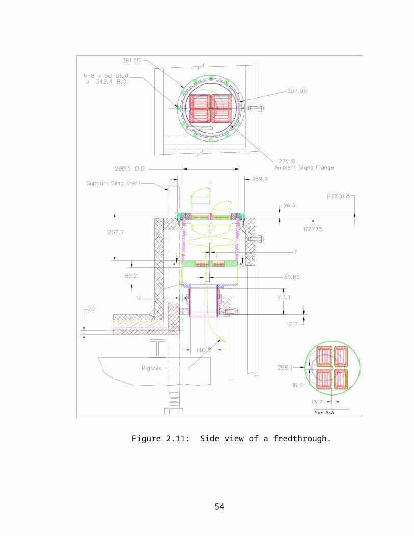
Figure 4.8: Data from two different scanner card tests on FT 23 – Mid 2. The plot shows a clear correlation in the different sections.

effect was found to corresponds to two different mother boards. This pattern is believed

to most likely derive from resistors that are either damaged or come from different

batches. Another possibility is that there is a link to the calibration line in the front

section. However, there is no convincing explanation that can truly account for these

effects.

59

There were also a few instances were an odd/even effect was measured in a few

places. It was found that the measured resistance of odd channels is systematically

higher than the measured resistance of the even channels in these areas. It is believed

that this problem could be derived from a bad ground connection when the scanner card

is plugged into the connectors

This thesis has presented results from the resistance measurements of the

complete electronics chains of the M-Wheel half of the EM barrel calorimeter. The result

of less than 0.1 % of the 58,386 channels operating outside of the parameters specified by

the collaboration indicates that this half of the barrel is within the acceptable limits in

order for it to operate properly in the ATLAS experiment. Therefore the M-Wheel half

of the barrel is ready to be sealed. The next steps will be to test the P-Wheel half of the

barrel. If it is also found to be within the 0.1 % limit, then the entire barrel can be sealed

and filled with the liquid argon, and tested under these cold conditions before it will be

inserted into the ATLAS detector.

60

APPENDIX

Table A.1a: List of all found problem channels by module (M00 – M07).

Module Description of problems

M00 Back 0 (FT00) : Clear Structure of 2 Ω.Front 3 (FT31) : channel 49 off by +10 %, channel 70 off by +10 %Front 4 (FT31) : channel 3 off by +1%, channel 85 off by +20 %Mid2 (FT31) : channel 127 off by +0.3 %

M01 Front 5 (FT02) : channel 4 off by +1 %M02 Back 0 (FT03) : channel 47 off by +0.4 %M03 Back 0 (FT06) : channel 55 dead (not common to TPA test; unknown

reason)M05 Front 6 (FT09) : channel 41 off by +1%

Calib (FT09) : channel 60 off by +10 %M06 Back 1 (FT12) : channel 0 off by –1%

channel 1 off by +0.3 % channel 4 and 5 off by +0.6 % channel 36 off by 10 %Mid 2 (FT12) : channel 0 off by +0.3 % 1 off by +1% 4 off by +1% 5 off by +1% 8 off by +1% 9 off by +1% 12 off by +1% 13 off by +4%Calib (FT12) : channel 68 off by +0.4 % (calibration line of middle problems cells) Looks like a HV problem.

M07 PS (FT13) : channel 8 off by + 1.5 %Back 1 (FT14) : channel 60 off by + 0.3 %

61

Table A.1b: List of all found problem channels by module (M08 – M15).

Module Description of problems

M08 PS (FT16) : channel 121 off by + 0.7 %M10 Back 1 (FT19) : channel 19 off by +2%

Mid 2 (FT19) : channel 110 off y +1.2 %Back 1 (FT20) : channel 11 off by +2%Mid 2 (FT20 ) : channel 22 off by 0.3 %

M12 Front 4 (FT24) : channels 76 and 78 off by –1.5 %channels 79, 80, 82 off by –0.2 %

M13 Front 2 (FT25) : channels 2 and 3 off –50 %Calib (FT25) : channel 34,35 off by –2% (connected to front problems)Mid 2 (FT26) : channel 42 off by –1%

M14 Front 6 (FT28) : channel 115 dead (common to TPA test)Back 1 (FT28) : channels 62 and 63 off by –50 %Mid 0 (FT28) : channel 19 off by +0.7 %

M15 Front 6 (FT29) : channel 62 off by +0.2 %Front 5 (FT30) : channel 70 off by +0.2 %

62

Table A.2: FT00 (M00)

ATI Position <R> () /R (%) Comments

FT00-1 PS 2030.8 0.029 FT00-2 Front 0 3038.2 0.021FT00-3 Front 1 3037.9 0.020FT00-4 Front 2 3037.7 0.022FT00-5 Front 3 3037.7 0.018 FT00-6 Front 4 3037.8 0.022FT00-7 Front 5 3038.1 0.020FT00-8 Front 6 3037.2 0.028FT00-9 Back 0 1061.5 0.048 Channels 47-63 and 111-127:

lower by ~2 Ω FT00-10 Back 1 1060.0

1039.1 2984.7

0.042 0.018 0.023

FT00-11 Mid 0 1061.3 0.026 FT00-12 Mid 1 1061.0 0.046 Structure same as Back 0 in 32

channelsFT00-13 Mid 2 735.9 0.025FT00-14 Mid 3 735.6 0.019FT00-15 Cal 86.3

110.4 249.3

0.10 0.13 0.05

63

Table A.3: FT01 (M01)

ATI Position <R> () /R (%) Comments

FT01-1 PS 2030.9 0.028FT01-2 Front 0 3038.7 0.018FT01-3 Front 1 3037.8 0.020FT01-4 Front 2 3038.0 0.021FT01-5 Front 3 3037.8 0.022FT01-6 Front 4 3037.7 0.022FT01-7 Front 5 3037.9 0.024FT01-8 Front 6 3037.6 0.019FT01-9 Back 0 1061.7 0.028FT01-10 Back 1 1061.6

1040.12984.9

0.0300.0220.016

FT01-11 Mid 0 1061.6 0.028FT01-12 Mid 1 1061.5 0.026 Odd/even on second connectorFT01-13 Mid 2 735.9 0.023FT01-14 Mid 3 735.4 0.025

FT01-15 Cal 86.2110.2249.2

0.140.180.05

64

Table A.4: FT02 (M01)

ATI Position <R> () /R (%) Comments

FT02-1 PS 2031.0 0.026FT02-2 Front 0 3039.0 0.019FT02-3 Front 1 3039.0 0.022FT02-4 Front 2 3038.3 0.029FT02-5 Front 3 3038.4 0.025FT02-6 Front 4 3038.2 0.021FT02-7 Front 5 3038.0 0.023 Channel 4: 3054 Ω; unknownFT02-8 Front 6 3038.3 0.019FT02-9 Back 0 1062.1 0.024FT02-10 Back 1 1061.7

1040.22985.0

0.0190.0160.015

FT02-11 Mid 0 1061.8 0.023

FT02-12 Mid 1 Missing measurementFT02-13 Mid 2 735.9 0.026FT02-14 Mid 3 735.4 0.021

FT02-15 Cal 86.0110.2249.1

0.150.170.05

65

Table A.5: FT03 (M02)

ATI Position <R> () /R (%) Comments

FT03-1 PS 2030.1 0.030FT03-2 Front 0 3038.5 0.020FT03-3 Front 1 3038.3 0.016FT03-4 Front 2 3038.6 0.029 First 64 channels: odd/even effectFT03-5 Front 3 3038.0 0.026FT03-6 Front 4 3038.5 0.020FT03-7 Front 5 3038.4 0.023FT03-8 Front 6 3037.7 0.024FT03-9 Back 0 1062.0 0.042 Channel 47: 1058.0 ΩFT03-10 Back 1 1061.8

1040.22984.7

0.0300.0260.022

FT03-11 Mid 0 1061.9 0.027FT03-12 Mid 1 1061.8 0.024FT03-13 Mid 2 736.1 0.024FT03-14 Mid 3 735.7 0.026

FT03-15 Cal 86.5110.6249.5

0.110.150.07

66

Table A.6: FT04 (M02)

ATI Position <R> () /R (%) Comments

FT04-1 PS 2031.2 0.025FT04-2 Front 0 3038.6 0.017FT04-3 Front 1 3040.1 0.043 Calibration lines effectFT04-4 Front 2 3038.1 0.024 Odd /even effect in 1st connectorFT04-5 Front 3 3038.4 0.018FT04-6 Front 4 3037.5 0.017FT04-7 Front 5 3038.1 0.017FT04-8 Front 6 3037.8 0.016FT04-9 Back 0 1062.4 0.025FT04-10 Back 1 1062.2

1040.72985.2

0.0250.0210.014

FT04-11 Mid 0 1062.1 0.024FT04-12 Mid 1 1061.7 0.029FT04-13 Mid 2 736.2 0.023FT04-14 Mid 3 735.8 0.023

FT04-15 Cal 86.5110.5249.4

0.110.110.08

67

Table A.7: FT05 (M03)

ATI Position <R> () /R (%) Comments

FT05-1 PS 2030.8 0.028FT05-2 Front 0 3038.4 0.021FT05-3 Front 1 3038.1 0.020FT05-4 Front 2 3038.2 0.018FT05-5 Front 3 3037.8 0.019FT05-6 Front 4 3037.5 0.026 Channel 115: 3035ΩFT05-7 Front 5 3037.8 0.017FT05-8 Front 6 3037.4 0.024FT05-9 Back 0 1061.6 0.050 47 - 63 and 111 – 127: 1 ΩFT05-10 Back 1 1061.4

1040.22984.4

0.0220.0170.022

FT05-11 Mid 0 1061.6 0.027FT05-12 Mid 1 1061.1 0.041 Structure same as Back 0 in 32

channelsFT05-13 Mid 2 735.8 0.023FT05-14 Mid 3 735.5 0.021

FT05-15 Cal 86.2110.4249.3

0.160.180.07

68

Table A.8: FT06 (M03)

ATI Position <R> () /R (%) Comments

FT06-1 PS 2030.9 0.027FT06-2 Front 0 3038. 3 0.021FT06-3 Front 1 3038.3 0.019FT06-4 Front 2 3038.4 0.014FT06-5 Front 3 3037.5 0.028 Calibration line highFT06-6 Front 4 3037.8 0.018FT06-7 Front 5 3037.6 0.019FT06-8 Front 6 3037.2 0.022FT06-9 Back 0 1061.5 0.030 channel 55: dead, structureFT06-10 Back 1 1061.4

1040.02984.6

0.0250.0120.018

FT06-11 Mid 0 1061.1 0.039 Structure same as Back 0 in 32 channels

FT06-12 Mid 1 1061.4 0.024FT06-13 Mid 2 735.9 0.037 Structure in 32 channelsFT06-14 Mid 3 735.5 0.025

FT06-15 Cal 86.3110.4249.4

0.130.140.06

69

Table A.9: FT07 (M04)

ATI Position <R> () /R (%) Comments

FT07-1 PS 2030.9 0.025FT07-2 Front 0 3038. 2 0.017FT07-3 Front 1 3038.3 0.023FT07-4 Front 2 3037.0 0.016FT07-5 Front 3 3037.9 0.017FT07-6 Front 4 3037.9 0.023FT07-7 Front 5 3037.5 0.022FT07-8 Front 6 3037.5 0.018FT07-9 Back 0 1061.8 0.027FT07-10 Back 1 1061.6

1040.32984.6

0.0250.0240.023

FT07-11 Mid 0 1061.6 0.028FT07-12 Mid 1 1061.6 0.027FT07-13 Mid 2 735.9 0.023FT07-14 Mid 3 735.6 0.018

FT07-15 Cal 86.3110.4249.2

0.120.140.07

70

Table A.10: FT08 (M04)

ATI Position <R> () /R (%) Comments

FT08-1 PS 2031.0 0.028FT08-2 Front 0 3038. 2 0.017FT08-3 Front 1 3037.8 0.024FT08-4 Front 2 3038.4 0.016FT08-5 Front 3 3038.0 0.022FT08-6 Front 4 3037.7 0.020FT08-7 Front 5 3037.7 0.020FT08-8 Front 6 3037.5 0.020FT08-9 Back 0 1061.7 0.025FT08-10 Back 1 1061.5

1040. 32984.7

0.0240.0140.018

FT08-11 Mid 0 1061.6 0.024FT08-12 Mid 1 1061.5 0.023FT08-13 Mid 2 735.9 0.022FT08-14 Mid 3 735.6 0.026

FT08-15 Cal 86.3110.4249.3

0.120.140.05

71

Table A.11: FT09 (M05)

ATI Position <R> () /R (%) Comments

FT09-1 PS 2031.0 0.028FT09-2 Front 0 3038. 1 0.020FT09-3 Front 1 3037.9 0.021FT09-4 Front 2 3038.2 0.025FT09-5 Front 3 3038.0 0.017FT09-6 Front 4 3037.4 0.023FT09-7 Front 5 3037.7 0.020FT09-8 Front 6 3037.1 0.025 Channel 41: 3051.5 ΩFT09-9 Back 0 1061.5 0.039 StructureFT09-10 Back 1 1061.1

1039.82984.6

0.0510.0490.015

two populationsIdem

FT09-11 Mid 0 1061.2 0.046 Structure same as Back 0 in 32 channels

FT09-12 Mid 1 1061.3 0.048 IdemFT09-13 Mid 2 735.9 0.023FT09-14 Mid 3 735.6 0.019

FT09-15 Cal 86.35110.5249.3

0.120.140.06

Channel 60: 93.4 Ω

72

Table A.12: FT10 (M05)

ATI Position <R> () /R (%) Comments

FT10-1 PS 2030.9 0.035 Channel 24: 2033.1 ΩChannel 110: 2027.8 Ω

FT10-2 Front 0 3037.8 0.019FT10-3 Front 1 3038.1 0.019FT10-4 Front 2 3037.6 0.022FT10-5 Front 3 3037.7 0.021FT10-6 Front 4 3037.6 0.022FT10-7 Front 5 3037.6 0.016FT10-8 Front 6 3037.1 0.026FT10-9 Back 0 1060.9 0.025FT10-10 Back 1 1060.7

1039.02984.6

0.0270.0260.021

FT10-11 Mid 0 1060.7 0.031FT10-12 Mid 1 1060.6 0.031FT10-13 Mid 2 735.8 0.022FT10-14 Mid 3 735.4 0.022

FT10-15 Cal 86.2110.3249.2

0.100.110.06

73

Table A.13: FT11 (M06)

ATI Position <R> () /R (%) Comments

FT11-1 PS 2030.9 0.031 Channel 64: 2034.5 ΩFT11-2 Front 0 3038.5 0.021FT11-3 Front 1 3038.3 0.017FT11-4 Front 2 3037.8 0.020FT11-5 Front 3 3037.7 0.024FT11-6 Front 4 3038.0 0.021FT11-7 Front 5 3037.7 0.017FT11-8 Front 6 3037.1 0.021FT11-9 Back 0 1061.6 0.025FT11-10 Back 1 1061.3

1039.92984.5

0.0210.0230.023

FT11-11 Mid 0 1061.5 0.026FT11-12 Mid 1 1061.4 0.023FT11-13 Mid 2 736.0 0.028FT11-14 Mid 3 735.4 0.019

FT11-15 Cal 86.2110.3249.2

0.120.130.04

74

Table A.14: FT12 (M06)

ATI Position <R> () /R (%) Comments

FT12-1 PS 2030.9 0.035 Channel 2: 2026.2 ΩFT12-2 Front 0 3038.7 0.024FT12-3 Front 1 3038.3 0.016FT12-4 Front 2 3038.0 0.021FT12-5 Front 3 3037.5 0.024FT12-6 Front 4 3038.3 0.022FT12-7 Front 5 3037.1 0.025FT12-8 Front 6 3037.2 0.018FT12-9 Back 0 1061.6 0.026FT12-10 Back 1 1061.4

1039.92984.7

0.043

0.0160.022

Channel 0: 1052 Ω, 1: 1064.8 Ω, 4 and 5: 1067 Ω

Channel 36: 1118.8 ΩFT12-11 Mid 0 1061.6 0.025FT12-12 Mid 1 1061.4 0.025FT12-13 Mid 2 735.8 0.036 Channel 0: 737 Ω, 1: 743 Ω, 4:

742 Ω, 5: 744 Ω, 8: 745 Ω, 9: 742.4 Ω, 12: 747.3 Ω, 13: 760.8 Ω

FT12-14 Mid 3 735.5 0.022FT12-15 Cal 86.2

110.3249.2

0.100.140.07 Channel 68: 248.4 Ω

75

Table A.15: FT13 (M07)

ATI Position <R> () /R (%) Comments

FT13-1 PS 2030.8 0.049 Channel 8: 2059.0 Ω, 9: 2042.5 Ω, 13-14: 2034 Ω, 92: 2024.1 Ω

FT13-2 Front 0 3038.4 0.018FT13-3 Front 1 3038.1 0.021FT13-4 Front 2 3038.3 0.018FT13-5 Front 3 3038.1 0.025FT13-6 Front 4 3037.4 0.024FT13-7 Front 5 3037.4 0.019FT13-8 Front 6 3037.3 0.019FT13-9 Back 0 1061.4 0.046 StructureFT13-10 Back 1 1061.1

1039.92985.0

0.0320.0170.018

Structure

FT13-11 Mid 0 1061.0 0.051 Structure same as Back 0 in 32 channels

FT13-12 Mid 1 1061.4 0.027FT13-13 Mid 2 735.8 0.025FT13-14 Mid 3 735.2 0.022

FT13-15 Cal 86.2110.3249.2

0.150.160.07

76

Table A.16: FT14 (M07)

ATI Position <R> () /R (%) Comments

FT14-1 PS 2030.5 0.025FT14-2 Front 0 3038.2 0.022FT14-3 Front 1 3038.1 0.017FT14-4 Front 2 3038.0 0.019FT14-5 Front 3 3038.5 0.026FT14-6 Front 4 3038.2 0.019FT14-7 Front 5 3037.7 0.024FT14-8 Front 6 3037.8 0.050 Unstable on 2nd connector: 2-3 ΩFT14-9 Back 0 1061.7 0.022FT14-10 Back 1 1061.5

1040.02984.4

0.0300.0140.067 Chan 60: 2995.2 Ω

FT14-11 Mid 0 1061.5 0.030FT14-12 Mid 1 1061.6 0.027FT14-13 Mid 2 735.8 0.022FT14-14 Mid 3 735.4 0.021

FT14-15 Cal 86.2110.4249.2

0.110.130.05

77

Table A.17: FT15 (M08)

ATI Position <R> () /R (%) Comments

FT15-1 PS 2030.9 0.026FT15-2 Front 0 3038. 3 0.018FT15-3 Front 1 3038.2 0.019FT15-4 Front 2 3038.0 0.019FT15-5 Front 3 3037.7 0.023FT15-6 Front 4 3037.8 0.017FT15-7 Front 5 3037.7 0.022FT15-8 Front 6 3038.6 0.051 Unstable: odd /even structureFT15-9 Back 0 1061.7 0.028FT15-10 Back 1 1061.5

1040.12984.6

0.0220.0140.014

FT15-11 Mid 0 1061.5 0.024FT15-12 Mid 1 1061.4 0.027FT15-13 Mid 2 736.0 0.025FT15-14 Mid 3 735.6 0.017

FT15-15 Cal 86.2110.3249.2

0.110.130.06

78

Table A.18: FT16 (M08)

ATI Position <R> () /R (%) Comments

FT16-1 PS 2030.8 0.029 Chan 121: 2043.6 ΩFT16-2 Front 0 3038. 4 0.016FT16-3 Front 1 3038.4 0.019FT16-4 Front 2 3038.1 0.018FT16-5 Front 3 3037.9 0.019FT16-6 Front 4 3037.5 0.020FT16-7 Front 5 3037.5 0.022FT16-8 Front 6 3037.3 0.020FT16-9 Back 0 1061.5 0.025FT16-10 Back 1 1061.4

1040.12987.1

0.0270.0260.022 Unknown

FT16-11 Mid 0 1061.4 0.028FT16-12 Mid 1 1061.2 0.024FT16-13 Mid 2 735.9 0.033FT16-14 Mid 3 735.5 0.029

FT16-15 Cal 86.1110.2249.1

0.180.180.04

Odd/evenOdd/even

79

Table A.19: FT17 (M09)

ATI Position <R> () /R (%) Comments

FT17-1 PS 2030.9 0.028FT17-2 Front 0 3038.4 0.017FT17-3 Front 1 3038.1 0.019FT17-4 Front 2 3037.8 0.027FT17-5 Front 3 3038.0 0.016FT17-6 Front 4 3037.8 0.019FT17-7 Front 5 3037.7 0.023FT17-8 Front 6 3037.7 0.024FT17-9 Back 0 1061.7 0.027FT17-10 Back 1 1061.4

1040.12984.7

0.0210.0200.019

FT17-11 Mid 0 1061.4 0.024FT17-12 Mid 1 1061.2 0.025FT17-13 Mid 2 736.0 0.027FT17-14 Mid 3 735.6 0.024

FT17-15 Cal 86.2110.3249.2

0.120.150.05

80

Table A.20: FT18 (M09)

ATI Position <R> () /R (%) Comments

FT18-1 PS 2030.7 0.025FT18-2 Front 0 3038.3 0.016FT18-3 Front 1 3038.2 0.021FT18-4 Front 2 3038.1 0.016FT18-5 Front 3 3038.0 0.017FT18-6 Front 4 3038.1 0.019FT18-7 Front 5 3037.6 0.022FT18-8 Front 6 3037.3 0.016 Damaged pin on channel 64 has

been repaired: 07/07/03FT18-9 Back 0 1061.6 0.026FT18-10 Back 1 1061.3

1040.02984.9

0.0210.0150.013

FT18-11 Mid 0 1061.4 0.028FT18-12 Mid 1 1061.3 0.027FT18-13 Mid 2 735.9 0.023FT18-14 Mid 3 735.4 0.026

FT18-15 Cal 86.2110.4249.3

0.160.180.06

81

Table A.21: FT19 (M10)

ATI Position <R> () /R (%) Comments

FT19-1 PS 2030.7 0.029FT19-2 Front 0 3038. 4 0.019 Chan 96: 3041.6 ΩFT19-3 Front 1 3038.6 0.021 Chan 127: 3041.7 ΩFT19-4 Front 2 3038.3 0.021FT19-5 Front 3 3038.1 0.021FT19-6 Front 4 3037.7 0.020FT19-7 Front 5 3037.8 0.025FT19-8 Front 6 3037.0 0.018FT19-9 Back 0 1061.7 0.026FT19-10 Back 1 1061.2

1039.82984.2

0.0230.0250.019

Chan 19: 1086 Ω

FT19-11 Mid 0 1061.4 0.025FT19-12 Mid 1 1061.4 0.026 Chan 110: 1073 ΩFT19-13 Mid 2 735.9 0.029FT19-14 Mid 3 735.4 0.022

FT19-15 Cal 86.0110.1249.1

0.170.160.06

82

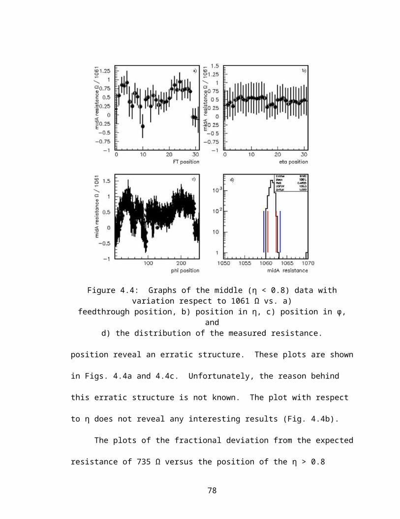
Table A.22: FT20 (M10)

ATI Position <R> () /R (%) Comments

FT20-1 PS 2030.7 0.029FT20-2 Front 0 3038.5 0.021FT20-3 Front 1 3038.7 0.028FT20-4 Front 2 3038.5 0.018FT20-5 Front 3 3038.3 0.019FT20-6 Front 4 3038.2 0.020FT20-7 Front 5 3038.2 0.026FT20-8 Front 6 3038.1 0.021FT20-9 Back 0 1061.2 0.025FT20-10 Back 1 1061.5

1040.02984.5

0.0220.0210.019

Chan 11: 1078.3 Ω

FT20-11 Mid 0 1061.5 0.026FT20-12 Mid 1 1061.5 0.023FT20-13 Mid 2 735.8 0.030 Chan 22: 737.5 ΩFT20-14 Mid 3 735.9 0.020

FT20-15 Cal 86.2110.3249.1

0.110.110.09

83

Table A.23: FT21 (M11)

ATI Position <R> () /R (%) Comments

FT21-1 PS 2031.0 0.025FT21-2 Front 0 3039.0 0.020FT21-3 Front 1 3039.2 0.022FT21-4 Front 2 3038.7 0.023FT21-5 Front 3 3038.1 0.016FT21-6 Front 4 3038.6 0.020FT21-7 Front 5 3038.4 0.021FT21-8 Front 6 3038.0 0.021FT21-9 Back 0 1063.0 0.025FT21-10 Back 1 1061.3

1040.02984.4

0.0250.0200.014

FT21-11 Mid 0 1061.8 0.025FT21-12 Mid 1 1061.6 0.025FT21-13 Mid 2 736.5 0.023FT21-14 Mid 3 736.2 0.019

FT21-15 Cal 86.2110.3249.5

0.100.130.05

84

Table A.24: FT22 (M11)

ATI Position <R> () /R (%) Comments

FT22-1 PS 2031.2 0.028FT22-2 Front 0 3039.4 0.022FT22-3 Front 1 3038.9 0.019FT22-4 Front 2 3039.1 0.022FT22-5 Front 3 3039.1 0.022FT22-6 Front 4 3038.9 0.022FT22-7 Front 5 3038.4 0.022FT22-8 Front 6 3038.6 0.021FT22-9 Back 0 1062.0 0.022FT22-10 Back 1 1061.7

1040.32984.7

0.0230.0160;025

FT22-11 Mid 0 1061.8 0.023FT22-12 Mid 1 1061.8 0.024FT22-13 Mid 2 736.5 0.031FT22-14 Mid 3 736.2 0.023

FT22-15 Cal 86.7110.8249.7

0.090.120.08

85

Table A.25: FT23 (M12)

ATI Position <R> () /R (%) Comments

FT23-1 PS 2030.8 0.026FT23-2 Front 0 3039.5 0.027FT23-3 Front 1 3039.1 0.031FT23-4 Front 2 3039.0 0.022FT23-5 Front 3 3039.0 0.026FT23-6 Front 4 3039.0 0.026FT23-7 Front 5 3038.4 0.021FT23-8 Front 6 3038.0 0.020FT23-9 Back 0 1061.8 0.026FT23-10 Back 1 1061.6

1040.22984.3

0.0250.0240.019

FT23-11 Mid 0 1061.8 0.032FT23-12 Mid 1 1061.7 0.025FT23-13 Mid 2 736.2 0.033 Measurement done with 2 scannersFT23-14 Mid 3 735.6 0.021

FT23-15 Cal 86.3110.4249.3

0.130.120.06

86

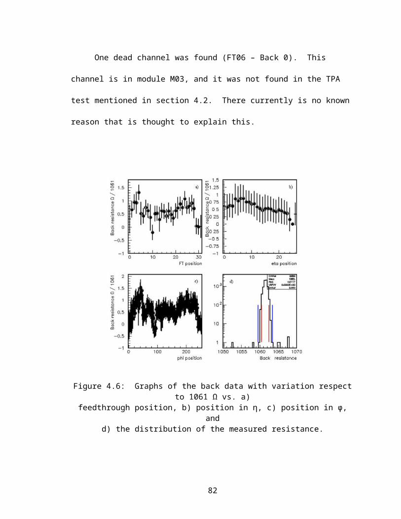
Table A.26: FT24 (M12)

ATI Position <R> () /R (%) Comments

FT24-1 PS 2031.1 0.029FT24-2 Front 0 3039.5 0.021FT24-3 Front 1 3039.3 0.018FT24-4 Front 2 3038.6 0.027FT24-5 Front 3 3039.0 0.017FT24-6 Front 4 3038.6 0.020 Chan 76,78: 2970 Ω, 79,80,82:

3033 ΩFT24-7 Front 5 3038.6 0.021FT24-8 Front 6 3038.1 0.014FT24-9 Back 0 1062.2 0.024FT24-10 Back 1 1061.9

1040.42985.8

0.0260.0160.017

FT24-11 Mid 0 1062.0 0.024FT24-12 Mid 1 1061.9 0.026FT24-13 Mid 2 736.5 0.020FT24-14 Mid 3 735.7 0.026

FT24-15 Cal 86.3110.4249.4

0.1040.0990.040

87

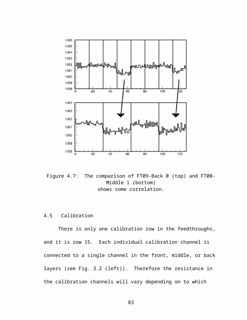
Table A.27: FT25 (M13)

ATI Position <R> () /R (%) Comments

FT25-1 PS 2031.1 0.025FT25-2 Front 0 3039.6 0.031 Second connector calibration:

Structure FT25-3 Front 1 3039.6 0.024FT25-4 Front 2 3038.2 0.037 Structure given by Rterm;

Channel 2, 3: 1523 Ω (checked by hand)

FT25-5 Front 3 3038.7 0.023FT25-6 Front 4 3038.6 0.022FT25-7 Front 5 3038.2 0.021FT25-8 Front 6 3038.3 0.020FT25-9 Back 0 1061.8 0.026FT25-10 Back 1 1061.7

1040.12985.6

0.0210.0170.024

FT25-11 Mid 0 1061.8 0.025FT25-12 Mid 1 1061.6 0.029FT25-13 Mid 2 736.3 0.030FT25-14 Mid 3 736.0 0.025

FT25-15 Cal 86.1110.1249.3

0.150.0490.075

Channel 34, 35: 108 Ω

88

Table A.28: FT26 (M13)

ATI Position <R> () /R (%) Comments

FT26-1 PS 2031.0 0.033 3.45, 3.73, 3.45, 3.73, 3.48, 3.75 ΩFT26-2 Front 0 3041.3 0.032FT26-3 Front 1 3038.8 0.025FT26-4 Front 2 3038.8 0.018FT26-5 Front 3 3038.6 0.020FT26-6 Front 4 3038.6 0.022FT26-7 Front 5 3038.5 0.026FT26-8 Front 6 3038.0 0.024FT26-9 Back 0 1061.9 0.028FT26-10 Back 1 1061.6

1040.22985.8

0.0240.0100.026 Chan 126: 2988 Ω

FT26-11 Mid 0 1061.8 0.026FT26-12 Mid 1 1061.7 0.026FT26-13 Mid 2 736.2 0.020 Chan 42: 729 ΩFT26-14 Mid 3 735.8 0.025

FT26-15 Cal 86.1110.2249.1

0.120.120.05

89

Table A.29: FT27 (M14)

ATI Position <R> () /R (%) Comments

FT27-1 PS 2030.9 0.025 3.54, 3.60, 3.53, 3.60, 3.56, 3.61 ΩFT27-2 Front 0 3041.1 0.027FT27-3 Front 1 3041.2 0.022FT27-4 Front 2 3041.1 0.022FT27-5 Front 3 3039.0 0.019FT27-6 Front 4 3041.0 0.022FT27-7 Front 5 3040.3 0.023FT27-8 Front 6 3039.1 0.033FT27-9 Back 0 1062.0 0.031FT27-10 Back 1 1061.8

1040.32987.6

0.0180.0140.024

FT27-11 Mid 0 1061.7 0.028FT27-12 Mid 1 1061.8 0.025FT27-13 Mid 2 736.2 0.023FT27-14 Mid 3 735.9 0.023

FT27-15 Cal 86.3110.5249.4

0.130.160.08

90

Table A.30: FT28 (M14)

ATI Position <R> () /R (%) Comments

FT28-1 PS 2030.9 0.024FT28-2 Front 0 3039.5 0.022FT28-3 Front 1 3041.5 0.021FT28-4 Front 2 3038.9 0.021FT28-5 Front 3 3038.7 0.023FT28-6 Front 4 3039.6 0.049 Odd/even of 1st; cal structure on 2nd

FT28-7 Front 5 3040.6 0.029FT28-8 Front 6 3038.4 0.020 Channel 115: MΩ’sFT28-9 Back 0 1061.9 0.027FT28-10 Back 1 1061.4

1040.22985.3

0.0330.0170.036 Chan 62, 63: 1630 Ω

FT28-11 Mid 0 1061.7 0.026 Chan 19: 1069 ΩFT28-12 Mid 1 1061.6 0.026FT28-13 Mid 2 736.1 0.025FT28-14 Mid 3 735.8 0.019

FT28-15 Cal 86.2110.4249.3

0.120.140.06

91

Table A.31: FT29 (M15)

ATI Position <R> () /R (%) Comments

FT29-1 PS 2030.7 0.030FT29-2 Front 0 3040.5 0.026FT29-3 Front 1 3040.2 0.022FT29-4 Front 2 3040.2 0.026FT29-5 Front 3 3040.8 0.035FT29-6 Front 4 3040.2 0.025FT29-7 Front 5 3039.9 0.023FT29-8 Front 6 3039.8 0.025 Channel 62: 3047 / 3040 ΩFT29-9 Back 0 1061.0 0.024FT29-10 Back 1 1061.0

1039.92984.4

0.0360.0200.018

FT29-11 Mid 0 1060.9 0.024FT29-12 Mid 1 1061.0 0.023FT29-13 Mid 2 735.9 0.026FT29-14 Mid 3 735.8 0.024

FT29-15 Cal 86.1110.2249.2

0.0130.0160.080

92

Table A.32: FT30 (M15)

ATI Position <R> () /R (%) Comments

FT30-1 PS 2030.7 0.032FT30-2 Front 0 3040.2 0.025FT30-3 Front 1 3040.7 0.030 Chan 90: 3036.4 ΩFT30-4 Front 2 3038.4 0.025FT30-5 Front 3 3038.1 0.031 Chan 70: 3044.2 ΩFT30-6 Front 4 3039.8 0.023FT30-7 Front 5 3039.9 0.023FT30-8 Front 6 3039.8 0.028FT30-9 Back 0 1061.1 0.026FT30-10 Back 1 1060.8

1039.42984.9

0.0270.0200.023

FT30-11 Mid 0 1061.0 0.028FT30-12 Mid 1 1060.9 0.023FT30-13 Mid 2 735.9 0.026FT30-14 Mid 3 735.3 0.020

FT30-15 Cal 86.2110.3249.2

0.110.130.06

93

Table A.33: FT31 (M00)

ATI Position <R> () /R (%) Comments

FT31-1 PS 2030.7 0.029FT31-2 Front 0 3038.3 0.026FT31-3 Front 1 3038.2 0.021FT31-4 Front 2 3037.4 0.026 Weak; calibration structureFT31-5 Front 3 3038.3 0.022 Chan 49: 3341.8 Ω, 70 : 3382.0 ΩFT31-6 Front 4 3037.8 0.023 Chan 3: 3052.3 Ω, 85: 3630.7 ΩFT31-7 Front 5 3037.6 0.016FT31-8 Front 6 3037.6 0.026FT31-9 Back 0 1061.0 0.040FT31-10 Back 1 1061.1

1040.02985.3

0.0440.0120.017

FT31-11 Mid 0 1060.7 0.027FT31-12 Mid 1 1061.0 0.038FT31-13 Mid 2 735.8 0.045 Chan 127: 738.6 ΩFT31-14 Mid 3 735.5 0.027

FT31-15 Cal 86.3110.4249.2

0.130.130.05

94

REFERENCES

1. D.E. Groom et al. (Particle Data Group), The European Physical Journal C15, 1 (2000) and 2004 edition available on the PDG WWW pages (URL: http://pdg.lbl.gov): S. Eidelman et al. (Particle Data Group), Phys. Lett. B592, 1 (2004).

2. G.D. Coughlan and J.E. Dodd, The Ideas of Particle Physics, 2nd ed. (Cambridge University Press, 1991).

3. ATLAS Collaboration, ATLAS Detector and Physics Performance Technical Design Report, vol. 1, CERN/LHCC/99-14 (1999).

4. K. Kleinknecht, Detectors for Particle Radiation, 2nd ed. (Cambridge University Press, 1998).

5. ATLAS Collaboration, ATLAS Liquid Argon Calorimeter Technical Design Report, CERN/LHCC/96-41 (1996).

6. ATLAS Collaboration, ATLAS Detector and Physics Performance Technical Design Report, vol. 2, CERN/LHCC/99-15 (1999).

7. D. Fournier and L. Serin, Experimental Techniques, LAL 96-57 (1996).

8. ALTAS Electromagnetic Liquid Argon Calorimeter Group, Construction, Assembly, and First Tests of the ATLAS Electromagnetic Calorimeter Barrel, Draft 0, to be submitted to Nucl. Instrum. Methods (2004).

95