TAM 203 Lab Manual - Andy Ruinaruina.tam.cornell.edu/Courses/Tam203_Spring09/Lab1... · TAM 203 Lab Manual This manual has evolved over the years. Contributors in the past two decades

TAM 203 Lab Manual

This manual has evolved over the years. Contributors in the past two decades include:Kenneth Bhalla, David Blocher, Jason Cortell, Drew Eisenberg, Jill Evensizer, Kwang YulKim, Richard Lance, Jamie Manos, Francis Moon, Dan Mittler, James Rice, Kevin Rompala,Andy Ruina, Bhaskar Viswanadham, and Alan Zehnder

Contents

TAM 203 Lab Introduction 5

Lab #1 - One Degree-of-Freedom Oscillator 11

Lab #2 - Two Degrees-of-Freedom Oscillator 31

Lab #3 - Slider-Crank Lab 45

Lab #4 - Gyroscopic Motion of a Rigid Body 55

TAM 203 Lab IntroductionLast Updated: January 22, 2008

PURPOSEThe laboratories in dynamics are designed to complement the lectures, text, and homework.They should help you gain a physical feel for some of the basic and derived concepts indynamics: force, velocity, acceleration, natural frequency, resonance, normal modes, andangular momentum. You will also get exposure to equipment and computers which you mayuse in the future. Some mathematics from courses you have taken recently or are now takingwill be used. We hope this will help you make the connection between mathematics andphysical reality that is essential to much of engineering. The labs may come either before orafter you cover the relevant material in lecture. Thus, they can be either a motivation forthe lecture material or an application of what you have learned depending on the timing.

COURSE INFORMATIONThere are four dynamics laboratories you will be performing during the semester:

1. One Degree-of-Freedom Oscillator

2. Two Degrees-of-Freedom Oscillator

3. Slider-Crank Mechanism

4. Gyroscopic Motion of a Rigid Body

Each of the four labs is taught for two or three weeks (depending on enrollment) in Thurston101. You will be scheduled to attend lab during one of the weeks. The dates for yourlaboratory section will be posted outside Thurston 101 and on the course website. In general,you will have a lab once every two or three weeks, but be aware that this may vary due toexam and break schedules.

NOTE: See the Administrative Assistant in Kimball 212 if you have any problemswith your lab schedule. You’ll need to get his or her approval for any changesso that the lab sections do not become overly full. Turning in a course changeform to the registrar is not enough.

LABORATORY ATTENDENCEYou are expected to attend the lab section you have signed up for. In the event of anexcused absence you must make-up the lab. All make-up labs must be arranged withyour TA. Your options for making-up labs are

1. Attend another of your lab TA’s lab sections.

5

6 TAM 203 Lab Introduction

2. Attend another lab TA’s lab section (requires permission from both lab TAs).

3. Attend the “Lab Make-Up Section” during the final week of the semester. Informationregarding the date and time of this section will be given in lecture near the end of thesemester.

If you show up for lab after it is under way, your lab instructor may ask you to leave and toperform the lab another time.

REQUIRED LABORATORY WORKThe laboratories will be done with physical equipment and some will also involve computersimulations. It is essential that you read through the lab (especially the proceduresection) before coming to lab. It is not necessary that you understand all of the materialperfectly before the lab period.

Prelab QuestionsEach lab has prelab questions to be answered before you come to lab. These questionsencourage you to review necessary theory and read through the laboratory procedure beforeattending the lab. Answers to prelab questions are due at the beginning of lab and will notbe accepted for credit later.

Laboratory NotesA rule of laboratory work is to keep a neat, complete record of what has been done, why itwas done, how it was done, and what the result was.

The success or failure of an experiment in a research laboratory often depends criticallyupon the record made of the experiment. The outcome of a poorly documented experimentbecomes a matter of personal recollection, which is not reliable enough to serve as a basisfor further work (especially by someone else). You should take copious notes. If in doubt,write it down. One can ignore what is written, but one can not resurrect that which wasnever recorded. Similarly, never erase in your lab notes. If an erroneous reading was made,strike it out with a single line and record the new data. You may later decide that it wasnot in error.

All lab notes, signed by your lab TA and in their original form, must be stapledto the back of your final lab report.

Lab ReportYour laboratory report should be typed using a word processor. This report should communi-cate clearly and convincingly what was demonstrated or suggested by the lab work. Your TAis looking for evidence of thought and understanding on your part. Your logic and methodsare as important as results or “correct” answers. It is essential that you provide informationand calculations which indicate how you arrived at your conclusions. It is permissible (anda good idea if you want a very good grade) to discuss observations and material relevant to

TAM 203 Lab Manual 7

the lab which is not specifically asked about in the questions.

Each report must begin with a cover page containing the following (with appropriate sub-stitutions for the words in quotes):

“NAME OF THE LAB”TAM 203By: “Your name and your signature (both partners if a joint report)”Performed: “Date”Performed with: “Name of person(s) with whom you performed the lab”Discussed lab with: “Names of people with whom you discussed the lab, and nature ofthe discussions”TA: “Lab TA’s name”TA signed the data on page: “Page #”

It is a good idea to include an introduction, abstract, or overview of the laboratory work youperformed as this will help communicate that you successfully grasp the purposes and goalsof the lab. It also gives you an opportunity to review your laboratory work before answeringspecific questions asked in the manual. If you deviate from the procuedure specified in themanual you should also state how and why you did so here.

You should concisely answer the questions that are asked and number them as they arenumbered in the lab manual. Include any necessary plots, data, or calculations (make sure toinclude the correct dimensional units). Your answers should be self-contained and presentedin an orderly fashion (i.e. the reader of the report should not have to refer back to thequestions that are asked, nor should he or she have to hunt through the report to find youranswers). While many questions require that you perform calculations, written explanationsof what you are doing and diagrams can be very helpful. Show all calculations that youperform in arriving at your answers. If you are performing repetitive calculations you needshow only one sample calculation.

Finally, at the end of your lab report you may want to include any observations, mistakesyou made, or suggestions you have in a concluding section.

When answering questions, percentage difference calculations can be used to quantify howwell experimental results agree with theoretical or expected values. Rather than writing “theexperimental results agree very well with the theoretical calculations,” this phrase can bechanged to make a quantifiable statement; “the experimental results are within 5 percent ofthe theoretical calculations.” Percentage difference is calculated as:

100%× (Value being compared - Reference value) / (Reference value)


While formal error analysis can be used if it is necessary to make a point, your answersshould include some discussion of the types and relative sizes of errors in your data.

All plots included with your lab report should be done on the computer using MATLAB(preferred) or Excel. Below are some guidelines for producing quality plots:

• All graphs should be titled and all axes labeled, with the appropriate units listed inparentheses.

• The independent variable should be placed on the horizontal axis.

• Numerical values on the axes should be set at reasonable intervals and scales chosenso that all of the data points can be displayed on the graphs.

• Curves should not be drawn between discrete data points unless the type of fittingused is explained and the equation of the curve given.

• On graphs with more than one curve a legend should be used to identify the curve.Data points can be enclosed by some symbol (i.e. circle, rectangle, etc.) to distinguishdifferent data sets.

Figure 0.1 is an example of how your graphs should appear. The MATLAB code thatproduced the graph is given below:

t = linspace(0,10,1000);

x = 5*cos(2*t);

v = -10*sin(2*t);

figure(1); hold on;

plot(t,x,’b’,’LineWidth’,2);

plot(t,v,’r--’,’LineWidth’,2);

grid on;

plot_title = title(’Plot of Position and Velocity vs. Time for Harmonic Oscillator’);

x_axis_label = xlabel(’Time (sec)’);

plot_legend = legend(’Position (m)’,’Velocity (m/s)’);

hold off;

set(plot_title,’FontWeight’,’bold’,’FontSize’,12);

set(x_axis_label,’FontWeight’,’bold’,’FontSize’,12);

set(plot_legend,’FontWeight’,’bold’,’FontSize’,12);

set(gca,’FontWeight’,’bold’,’FontSize’,12);

For help with producing log-log and semi-log plots with MATLAB, type help loglog, helpsemilogx, or help semilogy in the main MATLAB window.


0 1 2 3 4 5 6 7 8 9 10−10

−8

−6

−4

−2

0

2

4

6

8

10Plot of Position and Velocity vs. Time for Harmonic Oscillator

Time (sec)

Position (m)Velocity (m/s)

Figure 0.1: An example graph.

CREDIT AND GRADINGLab reports are due at 10:00 AM one week from the day you performed the lab unless your TAspecifies another time. Turn in reports in the boxes in the Don Conway room, Thurston 102.Put your report in the correct box corresponding to the TA in charge of your laboratorysection. Reports placed in incorrect boxes might not be found.

Each laboratory is graded out of 15 points. The grade breakdown for each lab report will bedetermined by your lab TA. This grade will be given to your recitation TA.

ACADEMIC INTEGRITYYour pre-lab answers and lab reports should be in your own words, based on your own under-standing and your own calculations. You are encouraged to discuss the material with otherstudents, friends, TAs, or even faculty. Any help you receive from such discussionsmust be acknowledged on the cover of your lab report, including the name ofthe person or persons and the exact nature of the help. Violations of this policy willbe reported to the academic integrity board.

You may, however, do a joint report with your lab partners (turn in one report for yourlab group). All partners get the same grade on the report but separate grades on pre-labquestions.

When you are done in the lab you must have your TA sign one of your data sheets. This sheetmust include the name of your lab partners and the time and date the lab was performed.


The TA will not sign this sheet until your work station is clean and all equipment is accountedfor. No lab reports will be accepted without this signed sheet.

Lab #1 - One Degree-of-Freedom OscillatorLast Updated: January 20, 2009

INTRODUCTIONThe mass-spring-dashpot is the prototype of all vibrating or oscillating systems. With vary-ing degrees of approximation, car suspensions, violin strings, buildings responding to earth-quakes, earthquake faults themselves, and vibrating machines are modeled as mass-spring-dashpot systems. This laboratory is aimed at demonstrating some of the basic conceptsof the mass-spring-dashpot system. In this lab you will collect data on the motion of twodifferent mass-spring-dashpot systems, and then use computer generated solutions of theequations of motion to determine system parameters. Phrases connected with some of thekey ideas are: natural frequency, resonance, forcing function, and frequency response.

PRELAB QUESTIONSRead through the laboratory instructions and then answer the following questions:

1. Find the general solution to (1.3) if the forcing term is given by Fs(t) = 0 and there isno damping (c =0), i.e. mx + kx = 0.

2. Repeat #1, this time numerically integrating the equation using Matlab. Choose m =1, k = 5, and integrate over the time period 0 ≤ t ≤ 10. Assume the mass starts fromrest with an initial displacement of x(0) = 1. What is the period of the oscillation?Turn in a plot and an m-file of your code.

3. Define in your own words: natural frequency, damping coefficient, underdamped, over-damped, resonance, and phase-shift.

THE MASS-SPRING-DASHPOT SYSTEMThe picture in Figure 1.1a shows a mathematical model of the laboratory mass-spring-dashpot, or one degree-of-freedom oscillator. A mass is supported by a spring and is con-strained to move in the e

x-direction. In this lab you will record the vertical motion of the

mass both with a fixed support (free vibration) and with the support oscillating vertically(forced vibration). The spring is modeled as linear, i.e. the force it applies is proportionalto its increase in length with proportionality constant k. The damping is also modeled aslinear, i.e. the force transmitted by the dashpot is proportional to the rate at which it isbeing stretched with proportionality constant c. The vertical displacement of the mass isx(t) and the vertical displacement of the support is xs(t).

Pictured in Figure 1.1b is a free body diagram of the mass. Neglecting gravity (Why can weneglect it? ), the mass has two forces acting on it in the e

x-direction:

Fsp(t) = k (xs − x) (1.1a)

11

12 Lab #1 - One Degree-of-Freedom Oscillator

Fd(t) = cx (1.1b)

where Fsp(t) is the spring force and Fd(t) is the damping force. The system is a one degree-of-freedom system because a single coordinate is sufficient to describe the complete state ofthe system. (The support displacement xs(t) does not count as a degree of freedom sinceit is specified by the motor position and is thus considered to be a given.) From Newton’s

Figure 1.1: Model and free body diagram of the mass-spring-dashpot system.

second law the equation of motion for this system is

{

∑

F}

· ex⇒ −Fd + Fsp = mx (1.2)

Plugging in the spring term (1.1a) and a damping term (1.1b), and rearranging terms thisbecomes

mx + cx + kx = Fs(t) (1.3)

where Fs(t) = kxs(t) is the specified “forcing function”. In this case the forcing function isthe amount the spring is additionally stretched due the support motion multiplied by thespring stiffness.

In the first part of this experiment you will attempt to determine the value of the viscousdamping constant c by measuring the rate at which oscillations decay towards zero, anexperiment called a ”ring-down test”. In addition, the system response to both free vibrationand forced vibration will be observed experimentally and through computer simulation.

A REAL-WORLD EXAMPLE: THE LOUDSPEAKERA speaker, similar to the ones used in many home and auto speaker systems, is one of manydevices which may be conveniently modeled as a one degree-of-freedom mass-spring-dashpot


system. The one you will observe in this lab is typical (see Figure 1.2). It has a plastic conesupported at the edges by a roll of plastic foam (the surround), and guided at the center bya cloth bellows (the spider). It has a large magnet structure and (not visible from outside) acoil of wire attached to the point of the cone which can slide up and down inside the magnet.When you turn on your stereo, it forces a current through the coil in time with the music,causing the coil to alternately repel and attract the magnet pushing the cone up and downin its housing. This results in the vibration of the cone which you hear as sound.

cone

mounting

�ange

spider

voice coil

frameelectrical

connections

magnet

structure

foam surround

( suspension )

Figure 1.2: Cross-sectional view of a speaker.

A simplistic view is that the cone and coil provide inertia (mx), the foam surround andclothe bellows act as a spring (kx), viscous damping comes from the cone moving throughthe air (cx), and the magnet provides external forcing Fs(t). Putting it all together we getthe familiar equation of motion of a driven mass-spring-dashpot system:

mx + cx + kx = Fs(t) (1.4)

Thus by appropriately choosing the parameters m, k, c and Fs(t) we can model the motionof the speaker as a mass-spring-dashpot system.

SOLVING THE EQUATIONS OF MOTIONOur goal is to find the motion of the mass, x(t), for a given forcing function Fs(t). Thetwo most important cases are free vibration, where Fs(t) = 0, and sinusoidal forcing, aspecific case of forced vibration where Fs(t) = kxs(t) = kAsupport cos ωt, where Asupport is thevibration amplitude of the support.

Recall that the differential equation governing the motion (1.3) is given by

mx + cx + kx = Fs(t) (1.5)

From ordinary differential equation theory we can write the general solution to (1.5) as thesum of a complimentary (also referred to as the transient or homogeneous) solution xc(t)and a particular solution, xp(t).


x(t) = xc(t) + xp(t) (1.6)

The homogeneous portion xc(t) is the solution to (1.5) with F (t) = 0 (and appropriate initialconditions). In this case, xc(t) goes to zero as t → ∞ - any initial motion of the mass willeventual be damped out if there is no external forcing. Thus the particular solution xp(t) iswhat is left as t → ∞ for any initial condition and includes the information about forcing.

In this section we are concerned with unforced vibrations, so we have x(t) = xc(t). We willdeal with xp(t) later. As you may have seen in other courses, we posit the solution to beof the form xc(t) = Aeλt (if this process seems unfamiliar to you, please review differentialequations). When we insert this into (1.5), we obtain the characteristic equation,

mλ2 + cλ + k = 0 (1.7)

which has roots given by the quadratic equation as,

λ1,2 =−c ±

√c2 − 4mk

2m(1.8)

Now, depending on the values of the parameters c,m, and k (specifically the discriminantc2 − 4mk), there are three situations encountered, and thus three different behaviors of thedisplacement x(t). These situations are:

• c2 − 4mk > 0: This produces two distinct real roots λ1 and λ2, and the solution isxc(t) = C1e

λ1t +C2eλ2t. This sytem is called overdamped– the system will slowly settle

down to xc(t) = 0 with no oscillations.

• c2 − 4mk = 0: This produces a repeated real root λ1 = −c/2m and the solution isxc(t) = C1e

λ1t + C2teλ1t. This system is called critically damped - the system will

quickly settle down to xc(t) = 0 with no oscillations. Why is the decay more rapid thanthe overdamped case?

• c2 − 4mk < 0: This produces a complex conjugate pair α ± iβ with α < 0 and thesolution is xc(t) = eαt [C1 cos(βt) + C2 sin(βt)]. This sytem is called underdamped–themass will oscillate, but the oscillations will decay with time according to the exponentialfactor (see Figure 1.3).

Naturally, the constants C1 and C2 will be determined from initial conditions for the speedand displacement of the mass.

A useful quantity (you will see why), termed the natural frequency ωn is defined as,

ωn =

√

k

m(1.9)


Underdamped Overdamped

Critically Damped

t

x

x0

Figure 1.3: Typical solutions for underdamped, overdamped, and critically dampedcases.

As you will show in prelab question (1), this is the system’s frequency of vibration whenthere is no damping (c = 0). Additionally, instead of employing the discriminant c2 − 4mkto describe the state of the sytem (over/under/critically damped) , it is convenient to definea damping factor, ζ, as

ζ =c

2√

mk(1.10)

ζ is defined in such a way that

• ζ > 1 is an overdamped system

• ζ = 1 is a critically damped system

• ζ < 1 is an underdamped system

Thus, ζ is a non-dimensional measure of the amount of damping in the system. In this lab,we will assume that both the mass-spring-dashpot system and the speaker areunderdamped. In fact we will assume ζ ≪ 1!

Using these definitions, we can restate the quadratic equation we found above in terms ofthe new variables, which yields (after some algebra)

λ1,2 = −ζωn ± ωn

√

ζ2 − 1 (1.11)


Since we are studying the underdamped system in the lab, we take ζ < 1 and find that theroots are

λ1,2 = −ζωn ± iωd (1.12)

where we defined the damped natural frequency (i.e. the frequency of oscillation with damp-ing) as ωd = ωn

√

1 − ζ2. Thus, the solution for the underdamped system is,

xc(t) = e−ζωnt [C1 cos(ωdt) + C2 sin(ωdt)] (1.13)

which can be restated as,xc(t) = Ae−ζωnt cos(ωdt − φ) (1.14)

where A =√

C21 + C2

2 , and φ = tan−1(−C2/C1) are two constants to be determined fromthe initial conditions.

THE LOGARITHMIC DECREMENT METHODIt is often important to measure how much damping there is in an engineering system. Theviscous damping constant, c, may be determined experimentally by measuring the rate ofdecay of unforced oscillations - this process is called a ”ring down” test. We define the loga-rithmic decrement, D, as the natural logarithm of the ratio of any two successive amplitudes:

D = ln

(

xn

xn+1

)

(1.15)

where xn and xn+1 are the heights of two successive peaks in the decaying oscillation (seeFigure 1.4). The larger the damping, the greater will be the rate of decay of oscillationsand the bigger the logarithmic decrement, D. To measure the logarithmic decrement D,we note that successive peaks occur on the decay envelope Ae−ζωnt when the periodic term,cos(ωdt−φ), takes on its maximum value of 1 (see Figure 1.4). Writing out the equation forthe decay envelope we have

xenvelope(t) = Ae−ζωnt (1.16)

Using this equation we now write the logarithmic decrement as the ratio of successive peaksof the periodic term

D = ln

(

xenvelope(t)

xenvelope(t + τd)

)

= ln

(

Ae−ζωnt

Ae−ζωn(t+τd)

)

= ln(

eζωnτd

)

= ζωnτd (1.17)

where τd is the period of the damped oscillation, i.e. τd = 2πωd

. We simplify this expression

by substituting in (1.10) for ζ and then solve for the damping constant c, yielding (algebraomitted)

c =2mD

τd

(1.18)

We can also obtain an equation for k from (1.17) , yielding

k =c2

(

1 + 4π2

D2

)

4m=

c2

4mζ2(1.19)


0 1 2 3 4 5 6 7 8

−1

−0.5

0

0.5

1

t

x(t)

xn+1

xn

τd

x0e− ζωn t

Figure 1.4: The logarithmic decrement method.

Thus, by doing a ”ring-down” test we can experimentally obtain values for Dand τd. Then using equations (1.18) and (1.19) and given the mass m, we canfind the damping constant c and spring constant k for a one degree-of-freedomoscillator.

FORCED VIBRATIONS AND FREQUENCY RESPONSEOften a system is periodically forced and we are interested in how it will respond, e.g. thetires on your car going over evenly spaced ruts in the road jostles the car. In this section,we will solve the equation of motion (1.3) for the forced case and examine the phase andamplitude of the response. We assume that the support is driven harmonically such that theexciting force on the mass is F (t) = Fdrive cos ωt (i.e. the vibration amplitude of the supportis Asupport = Fdrive

k). The equation of motion (1.3) now becomes

x + 2ζωnx + ω2nx =

Fdrive

mcos ωt (1.20)

Note: This is the same equation of motion from before (1.5) but in terms of the new variablesfrom the previous section. Now we will only be interested in the steady-state oscillation thatwill be left after the transient response dies out, i.e. xp(t). We take the solution to be of theform,

xp(t) = Aresponse cos (ωt − φ) (1.21)

where Aresponse is the amplitude of oscillation of the mass and φ is the phase of the dis-placement x(t) with respect to the exciting force F (t). We should expect that the amplitude


Aresponse and phase φ of the response depends on how quickly (ω) and with what force (Fdrive)we drive the system. We can solve for φ(ω, Fdrive) and Aresponse(ω, Fdrive) by plugging ourguess at the solution (1.21) into the equation (1.20) and use the linear independence of cos ωtand sin ωt. Don’t worry about the algebra, the results are given below:

φ(ω) = arctan2ωωnζ

ω2n − ω2

; 0 ≤ φ ≤ π (1.22)

Aresponse(ω)

Fdrive

=1m

√

(ω2n − ω2)2 + 4ω2ω2

nζ2

(1.23)

Note that the phase of the response is independent of how hard we drive the system, thoughif we drive it twice as hard, the response amplitude is twice as big. How the system responsedepends on the drive frequency (ω) and system parameters (ωn, ζ) is a bit more complicated,and the best way to understand it is with a graph. In Figure (1.5) we assume the supportoscillates with unit amplitude xs(t) = cos ωt, thus Fdrive = k, and plot the response amplitudeand phase as a function of the drive frequency (ω) for different amounts of damping (ζ).

2

4

6

8

10

Res

pons

e A

mpl

itude

(A

)

Pha

se L

ag (

φ)

ζ = 0.05ζ = 0.1ζ = 0.2ζ = 0.4

ωn

ωn

0.1 ωn

10 ωn

10 ωn

0.1 ωn

π

π /2

Figure 1.5: The system response x(t) = A cos ωt + φ as a function of forcing frequencyω, for various amounts of damping ζ

Note from the plot that:

• for very low drive frequencies (ω ≪ ωn) the response is synchronized with the driving.The phase lag (φ) is 0, and the amplitude of vibration of the mass is the same as theamplitude of vibration of the support. What is the physical argument for this?

• for drive frequencies near ωn the response amplitude is at a maximum and the phaselag is π

2.


• for very high drive frequencies (ω ≫ ωn) the response is completely out of phase withthe driving and the amplitude of vibration goes to zero. What is the physical argumentfor why the amplitude vanishes?

• the less damping there is, the sharper the change in phase is, and the greater theresponse near ωn.

RESONANCEResonance as defined by Merriam-Webster is a vibration of large amplitude in a mechanicalor electrical system caused by a relatively small periodic stimulus of the same or nearly thesame period as the natural vibration period of the system. For an undamped system, reso-nance occurs when we force the system at its natural frequency, i.e. ω = ωn, and the responseis unbounded (note how the peaks in Figure 1.5 increase as ζ → 0). However, resonance ina damped mass-spring-dashpot system does not occur when the forcing frequency is exactlythe undamped natural frequency ωn, and the response is not unbound but simply a maxi-mum. To find the resonant frequency, ωr, we maximize the response’s amplitude (1.23) bydifferentiating Aresponse(ω) with respect to the forcing frequency ω (holding everything elsefixed)and setting it equal to zero.

dAresponse

dω

∣

∣

∣

∣

ω=ωr

= 0 ⇒ ωr = ωn

√

1 − 2ζ2 (1.24)

Note for small damping (ζ ≪ 1) we have√

1 − 2ζ2 ∼ 1 and so the resonant frequency ωr

and the natural frequency ωn are approximately equal ωr ≃ ωn.

PHASE DIAGRAMS In our experiment we will need a way to tell if the system is nearresonance without adjusting the forcing frequency until the response is maximized. One easyway is to examine the phase lag(φ). It can be shown that when we force the system at it’snatural frequency (ωn) that the phase is, φ = π

2(Verify this by inspection (see Figure 1.5)

or directly from (1.22). The corresponding phase diagram will then be a circle (If you areinterested, further details on what a phase diagram is can be found in the appendix). Notefrom the previous section that for small damping ωn ≃ ωr, and so for the systems in our labwhen we see a circle we know we are at (or very close to) resonance.

LABORATORY SET-UP

• Mass-Spring-Dashpot SystemThe apparatus consists of a laboratory-model mass-spring-dashpot system with dis-placement transducers (Linear Variable Differential Transformers or LVDTs) for mea-suring x(t) and xs(t). The output from the LVDTs is communicated to the computervia the data acquisition board. An electric motor and controller, acting through ascotch yoke, enable a sinusoidal forcing function to be applied to the system. Notethat the controller dial readings are arbitrary; frequency and period data must beobtained from your computer plots.


• LoudspeakerThe apparatus consists of a speaker on a stand with one LVDT to measure cone dis-placement. Waveforms are generated by the computer, amplified, and sent througha resistor to drive the speaker. The computer is also used to measure current flowthrough the speaker and displacement of its cone (using the attached LVDT).

Please follow all safety precautions. Keep long hair and loose clothing well away fromthe electric motor, pulleys, and other moving parts.

• Using the LabView SoftwareThe four programs you will be using in the first part of the lab are: FreeAcq (Figure 1.6)for making measurements of the unforced system; FreeSim (Figure 1.7) for simulationof the same; ForcedAcq (Figure 1.8) for measurements of the system with a sinusoidalforcing function; and ForcedSim (Figure 1.9) which may be used for simulation of theforced system. Although somewhat different in appearance and function, the programsshare many key features. The SpeakerAcq (Figure 1.10) program used in the secondpart of the lab is also similar.

Figure 1.6: The FreeAcq program.


Figure 1.7: The FreeSim program.

Figure 1.8: The ForcedAcq program.


Figure 1.9: The ForcedSim program.

Figure 1.10: The SpeakerAcq program.


To run the program, you must hit the white arrow in the top left of the screen. Ifthis arrow is black, that means that the program is already running. For the dataacquisition programs, a green box on top will define the amount of time for which theprogram will record after hitting the arrow. To reset the data acquisition, press STOP

without Saving and then press the white arrow to begin again.

After getting data, pressing the Save and STOP button stores your current data ondisk. The data file is only used by the simulation programs FreeSim and ForcedSim-it is not available to the data acquisition programs.

You may find it convenient to obtain numerical data from your plots using the cursors,rather than using a ruler. Two cursors are available, one indicated by a circle andone by a square. To use a cursor, use the mouse to drag it to the point you want tomeasure. If your cursor has vanished off the screen, you can enter an on-screen positionfor it into the x and y display boxes, and it will reappear in the desired location. Youcan also lock the cursor to a curve by clicking the lock icon. Zoom and other featuresare available for the cursors and graphs; see the LabView manual for details.

PROCEDURE

• Free Vibration, Mass-Spring-Dashpot

1. First you will measure the free vibration of the mass.

– Start up the FreeAcq program. The data acquisition programs automaticallyconvert the voltage output of the LVDTs to meters. To do this, they needa set of conversion factors, which are on a label on the mass-spring-dashpotbase board. Make sure that the sensitivity and offset values on the left handside of the window match the values listed on a small sheet of paper in frontof the apparatus, and enter your name in the box provided. Set the dataacquisition time to 6 seconds.

– Pull down the mass and hold it still, then press the white run arrow in thetop left of the toolbar and immediately release the mass.

– Repeat this procedure until you have a nice oscillation over the 6 seconds.Please note that the zero position is somewhat arbitrary. You will need totake data long enough for the mass to stop oscillating in order to have a goodzero reference.

– Save your best oscillation on disk by pressing the Save and STOP button.

2. Next you will measure the logarithmic decrement D and estimate the spring stiff-ness k and damping coefficient c.

– Start the FreeSim program, and add the measured data to the graph bypressing the Measurement Data switch above the graph. Set k = 0 to get thesimulated data out of the way.


– Using the cursors, measure the logarithmic decrement D and the period ofthe damped oscillation τd for each set of successive peaks (at least 3).

– Using these measured values, and the mass m, calculate the damping constantc and spring stiffness k (The mass of the weight and spring are written at thebase of the setup. For your ’m’ use the total of the weight and spring).

– Make a print-out of your curve.

3. Finally, you will simulate the free vibration of the mass-spring-dashpot systemand verify your estimate of the system parameters. Simulate unforced motion byinputting the values of m, k, and c that you just determined into the FreeSimprogram.

– Adjust the initial condition and viewing parameters (t(0), h, x(0), D) to fityour data. Don’t change k or c.

– Make a print-out.

– Now see if you can adjust k and c to get a better agreement. Take note ofwhat aspects of the graph change when you change each of the parameters kand c.

– Make another print-out.

• Forced Vibration, Mass-Spring-Dashpot

1. Here you will be recording the motion of the mass as it undergoes sinusoidalforcing.

– Start the ForcedAcq program.

– Set the acquisition time to 30 seconds, start the data acquisition and turn onthe motor. Two graphs will be displayed. The left one contains two plots.One is a plot of the mass position x(t) vs. time and the second one is a plotof the spring support position xs(t) vs. time. The right graph plots the phasediagram.

– For at least five different forcing frequencies get nice plots of several cycles ofmotion (see instructions below). Make sure to save each data set to disk inorder to analyze them in the ForcedSim program. Print-outs are not necessarybut may be helpful.

– To acquire data, set the data acquisition time to 10 seconds and run theprogram in order to find the desired drive frequency. Then hit STOP without

SAVING. Reduce the data acquisition time to ∼ 1 second (or atleast longenough to get one whole cycle) and then run the program again. This timehit SAVE and STOP.Reducing the acquisition time will reduce demand on theserver and save you time doing analysis. Forcing frequencies should include:

∗ The lowest frequency for which the motor runs smoothly.

∗ A frequency just lower than resonance.

∗ Resonance. (Hint: we tell from the phase diagram that it is at resonance)


∗ A frequency just higher than resonance.

∗ A very high frequency.

2. Next we will simulate the forced vibration of the mass-spring-dashpot system.

– Open the ForcedSim program.

– Turn on the measured data switch to view your saved data. To change thecurrent measured data set you must close and then re-open the ForcedSimprogram. Once experimental data is loaded, make your necessary measure-ments (see below) using the computer cursors.

– For each of the five frequencies you will need to measure and record thefollowing data:

∗ damped period (τd)

∗ forcing function amplitude (F ) (Note: you will actually see Fk, the ampli-

tude of the support oscillation)

∗ mass motion amplitude (A)

∗ phase-lag between the forcing function and the resulting mass motion (φ)

You may also want to save the data to a USB storage device or write it to a CD forlater analysis. To do this just copy the text files of the desired data onto your storagedevice.

• Vibration of a Speaker

• In the last part of the lab, you will experimentally fit the parameters k and c for aspeaker by measuring the shift in resonance frequency due to the addition of a knownmass.

1. First you will force the loudspeaker at its resonant frequency in order to experi-mentally determine the mass m and spring constant k of the loudspeaker.

– Set the Waveform control to Sine and the Amplitude control to 2. Leavethe DC Offset control set to 0. Set the data acquisition time to 0.1 seconds.The CH 0 Offset and CH 1 Offset controls may be used to adjust the plotsvertically if necessary.

– Turn on the waveform generator and data acquisition switches and adjustthe Frequency control value until you observe resonance of the speaker cone.To change the frequency you must press STOP without Saving, enterthe desired frequency and then start the program again in order toobserve the new frequency.

– Make a print-out and record the frequency (note the need to convert from Hzto rad/sec).

Recall that the resonant frequency depends on both the mass m and spring stiff-ness k. By measuring the resonant frequency you cannot solve for both m andk uniquely. However, if you also measure the resonant frequency when the mass


is changed a known amount then you will have 2 equations ( i.e. (1.9), assumeωr ∼ ωn) for 2 unknowns (m, k) in terms of measured data (ω1r, ω2r,△m). Nowmeasure the mass of the rubber weight and then carefully press it onto the LVDTshaft. The best way is to spread the weight open, position it, and release it.

– Find the new resonant frequency, and record the mass of the rubber weight.

– Make a print-out and record the frequency (note the need to convert from Hzto rad/sec).


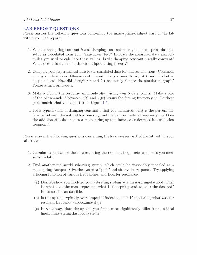
LAB REPORT QUESTIONSPlease answer the following questions concerning the mass-spring-dashpot part of the labwithin your lab report:

1. What is the spring constant k and damping constant c for your mass-spring-dashpotsetup as calculated from your ”ring-down” test? Indicate the measured data and for-mulas you used to calculate these values. Is the damping constant c really constant?What does this say about the air dashpot acting linearly?

2. Compare your experimental data to the simulated data for unforced motions. Commenton any similarities or differences of interest. Did you need to adjust k and c to betterfit your data? How did changing c and k respectively change the simulation graph?Please attach print-outs.

3. Make a plot of the response amplitude A(ω) using your 5 data points. Make a plotof the phase-angle φ between x(t) and xs(t) versus the forcing frequency ω. Do theseplots match what you expect from Figure 1.5.

4. For a typical value of damping constant c that you measured, what is the percent dif-ference between the natural frequency ωn and the damped natural frequency ωd? Doesthe addition of a dashpot to a mass-spring system increase or decrease its oscillationfrequency?

Please answer the following questions concerning the loudspeaker part of the lab within yourlab report:

1. Calculate k and m for the speaker, using the resonant frequencies and mass you mea-sured in lab.

2. Find another real-world vibrating system which could be reasonably modeled as amass-spring-dashpot. Give the system a“push” and observe its response. Try applyinga forcing function of various frequencies, and look for resonance.

(a) Describe how you modeled your vibrating system as a mass-spring-dashpot. Thatis, what does the mass represent, what is the spring, and what is the dashpot?Be as specific as possible.

(b) Is this system typically overdamped? Underdamped? If applicable, what was theresonant frequency (approximately)?

(c) In what ways does the system you found most significantly differ from an ideallinear mass-spring-dashpot system?


CALCULATIONS & NOTES


Appendix: Phase Diagrams A phase diagram is a plot which contains the forcingfunction Fs(t) on the y-axis and the response function x(t) on the x-axis. The phase diagramis a graphical representation of the relative phase of the forcing and motion. Each point onthe plot tells us both where we are in the drive cycle y(t) and on the response cycle x(t).Time is a parameter that moves us around on the diagram. Since we are only interested inthe phase, we scale each term by its amplitude. Thus on our phase diagram we would plotthe parametric function

y(t) = cos(ωt) (1.25)

x(t) = cos(ωt − φ) (1.26)

When we force the system at ωn ≃ and the phase is φ = π2

as shown before, we have:

y(t) = cos(ωt) (1.27)

x(t) = cos(ωt − π

2) (1.28)

Using the following trigonometric identities:

cos2 ωt + sin2 ωt = 1 (1.29)

cos(ωt − π

2) = sin ωt (1.30)

We can establish the following relationship for our phase plot:

x2(t) + y2(t) = 1 (1.31)

Hopefully you will recognize this equation as the parametric form of the equationfor a circle! Thus, when we force the system at its natural frequency which is very close toits resonant frequency the phase diagram is a circle.


Documents

TAM 203 Lab Manual - Andy Ruinaruina.tam.cornell.edu/Courses/Tam203_Spring09/Lab1... · TAM 203 Lab Manual This manual has evolved over the years. Contributors in the past two decades