Talk and Action:

What Individual Investors Say and What They Do∗

Daniel Dorn†

Gur Huberman‡

This draft: December 16, 2003

ABSTRACT

Combining survey responses and trading records of clients of a German retailbroker, this paper examines some of the causes for the apparent failure to buyand hold a well-diversified portfolio. Investors who report being wealthier andmore experienced hold better diversified portfolios and churn their portfolios less;irrationality, or the cost of informed participation in the stock market, appearsto decrease in wealth and experience. Self-assessed risk tolerance, however, is thesingle most important determinant of both portfolio diversification and turnover;investors who report being more risk tolerant hold less diversified portfolios andtrade more aggressively. Risk-tolerant investors also believe that that they cancontrol risk which suggests that risk tolerance serves as a proxy for an “illusion ofcontrol” and thus overconfidence. The results appear robust to specification errordue to sample selection and are not driven by entertainment accounts.

∗We thank Carol Bertaut, Anne Dorn, Larry Glosten, Will Goetzmann, Charles Himmelberg, WeiJiang, Alexander Ljungqvist, Theo Nijman, Paul Sengmueller, Elke Weber, and participants at the 2003European Finance Association meetings in Glasgow for their comments.

†LeBow College of Business, Drexel University; 208 Academic Building; 101 North 33rd Street;Philadelphia, PA 19146; Email: daniel.dorn@drexel.edu

‡Graduate School of Business, Columbia University; 807 Uris Hall; 3022 Broadway; New York, NY10027; Email: gh16@columbia.edu

I. Introduction

Traditional finance theory predicts that individual investors simply buy and hold the

market portfolio, or at least a well-diversified portfolio of stocks. The typical retail in-

vestor doesn’t; most of those who hold stocks directly hold just a handful of stocks rather

than a diversified portfolio (see, e.g., Blume and Friend (1975) and the 1998 U.S. Survey

of Consumer Finances (SCF)). More disturbingly still, many retirement plan partici-

pants allocate a substantial fraction of their discretionary retirement funds to company

stock (see Benartzi (2001)).

The second part of the buy-and-hold prediction is that market participants do not

churn their portfolios. This prediction also appears to be strongly rejected in the data.

Griffin et al. (2003)) attribute most of the turnover of Nasdaq 100 stocks during 2000

and 2001 – well above 200% (see NYSE (2001)) – to individual investors.1 Using trad-

ing records for a sample of U.S. discount brokerage clients, Barber and Odean (2000)

document that the frequent traders perform about as well as other investors ignoring

trading costs, but do considerably worse when trading costs are taken into account.

Combining survey responses and trading records of clients of a German retail broker,

this paper examines some of the causes for the apparent failure to buy and hold a well-

diversified portfolio. The unique data set allows us to relate the clients’ self-reported

characteristics derived from survey responses to their actual financial decisions inferred

from the trading records.

2

Does irrationality disappear with wealth or other proxies of investor sophistication?

A simple explanation for the poor diversification and churning of individual investor

portfolios is widespread ignorance, or, equivalently, considerable effort associated with

informed participation in the stock market. The sample investors report their total

wealth and the length of their stock market experience both of which can be interpreted

as measures of investor sophistication. Wealthier and more experienced investors tend

to hold better diversified portfolios and churn their portfolios less which suggests that

irrationality, or the cost of becoming an informed participant, decreases in wealth and

experience. Moreover, investors with a preference for the familiar – measured as the

fraction of the portfolio held in domestic stocks, either directly or through mutual funds,

or the distance between the investor and his portfolio relative to the distance between

the investor and the market portfolio (see Coval and Moskowitz (1999)) – tend to buy

and hold a concentrated portfolio of near-by stocks.

These results contribute to the emerging literature that examines whether investors

who are judged “sophisticated” by socio-economic attributes such as income or occupa-

tional choice are less prone to underdiversify (see Goetzmann and Kumar (2002)), hang

on to losers and sell winners (also known as the disposition effect; see Odean (1998a) and

Dhar and Zhu (2002)), and make locally biased investments (see Zhu (2002)). While the

cited studies focus on common stock transactions by similar samples of U.S. discount

brokerage clients, this paper considers holdings and trades in stocks and mutual funds of

German brokerage clients. The inclusion of mutual funds, in particular, yields sharper

inferences about portfolio diversification as mutual funds offer a simple and cheap way

to diversify across assets and regions.

3

Do overconfident investors violate the buy-and-hold recommendation as suggested

by Odean (1998b)? Survey responses allow us to construct direct measures of overconfi-

dence, such as an investor’s tendency to attribute gains to his skill and losses to bad luck

– essential features of the self-attribution bias, modelled as a driver of overconfidence by

Daniel et al. (1998) and Gervais and Odean (2001) – or such as the discrepancy between

self-assessed knowledge and the performance on a short quiz contained in the survey. In-

terestingly, these measures of overconfidence are essentially unrelated to other personal

attributes and fail to explain differences in portfolio diversification and turnover.

Remarkably, self-reported risk tolerance does the best job of explaining differences

in both portfolio diversification and portfolio turnover across individual investors. From

the vantage point of traditional finance theory, the positive correlation between risk

tolerance and diversification is surprising, as both risk-tolerant and risk-averse investors

should diversify away idiosyncratic risk. We find that investors who report being risk-

tolerant are also more prone to believing that risk can be controlled which suggests that

self-assessed risk tolerance also serves as a proxy for an “illusion of control”, that is,

overconfidence about one’s ability to affect chance outcomes (see Langer (1975)).

So far, tests of the overconfidence hypothesis have been inconclusive. Barber and

Odean (2001) use gender as a proxy for overconfidence, citing psychological research

suggesting that male investors are more overconfident than their female counterparts.

They document that male clients at a U.S. discount brokerage indeed trade more which

they interpret as support for the overconfidence hypothesis. Subsequent studies con-

struct overconfidence measures from survey responses and relate them to the propensity

to trade inferred from brokerage records (Glaser and Weber (2003)) or from a trad-

ing experiment (Biais et al. (2002)). The two studies find little or no relation between

measures of overconfidence and trading intensity.

4

Do investors appear to be poorly diversified and churn their portfolios because we

only observe a subset of their decisions and financial assets? A criticism commonly

levelled against field studies of investor behavior is that the results may be driven by

so-called entertainment accounts – accounts that are set aside for entertainment pur-

poses and are small relative to the investor’s unobserved holdings. Because the sample

investors examined in this paper report estimates of their wealth and the allocation of

their wealth across different asset classes such as financial assets and real estate, it is

possible to identify accounts that are likely to be important to the investor because they

represent a large fraction the investor’s wealth (a typical portfolio in the sample accounts

for one third of the investor’s wealth and more than half of his wealth held in financial

assets). Portfolios that are important to their holders are better diversified and churned

less though they are still a far cry from well-diversified buy-and-hold portfolios. The

results of the paper are robust to controlling for the estimated account-to-wealth ratio.

The remainder of the paper proceeds as follows: Next is a description of the trans-

action records and the survey data. Section Three summarizes demographic, socio-

economic, and subjective attributes of the survey respondents. Section Four compares

self-reported behavior with actual behavior by relating attributes and attitudes of the

sample investors to their actual behavior inferred from the trading records. Section Five

concludes.

II. Data

The analysis in this paper draws on transaction records and questionnaire data obtained

for a sample of clients at one of Germany’s three largest online brokers. “Online” refers

5

to the broker’s ability to process online orders; customers can also place their orders

by telephone, fax, or in writing. The broker could be labelled as a “discount” broker

because no investment advice is given. Because of their low fees and the width of their

product offering, German online brokers attract a large cross-section of clients ranging

from day-traders to retirement savers (during the sample period, the selection of mutual

funds offered by online brokers is much greater than that offered by full-service brokers

– typically divisions of the large German universal banks that are constrained to sell the

products of the banks’ asset management divisions). In June 2000, at the end of our

sample period, there were almost 1.5 million retail accounts at the five largest German

discount brokers (see Van Steenis and Ossig (2000)) – a sizable number, given that the

total number of German investors with exposure to individual stocks at the end of 2000

was estimated to be 6.2 million (see Deutsches Aktieninstitut (2003)).

A. Brokerage records

Complete transaction records from the account opening date (as early as January 1,

1995) until May 31, 2000 or the account closing date – whichever comes first – are avail-

able for all prospective participants in the survey, regardless of whether they choose to

participate in the survey or not. With these transaction records, client portfolios can be

reconstructed at a daily frequency. The typical record consists of an identification num-

ber, account number, transaction date, buy/sell indicator, type of asset traded, security

identification code, number of shares traded, gross transaction value, and transaction

fees. In principle, brokerage clients can trade all the bonds, stocks, and options listed

on German exchanges, as well as all the mutual funds registered in Germany. Here,

the focus is on the investors’ individual stock and mutual fund holdings and trades for

which Datastream provides comprehensive daily asset price coverage: stocks on Datas-

6

tream’s German research stocks list, dead or delisted stocks on Datastream’s German

dead stocks list, and mutual funds registered either in Germany or in Luxembourg. As of

May 2000, the lists contain daily prices for 8,213 domestic and foreign stocks and 4,845

mutual funds. These stocks and mutual funds represent over 90% of the clients’ holdings

and 80% of the trading volume, with the remainder split between bonds, options, and

unidentified stocks and mutual funds.2

Stocks can be classified as domestic or foreign stocks because the first two digits of

the stock’s International Security Identification Number (ISIN) identify the country in

which the company is registered. Mutual funds can be classified into domestic or foreign

funds because the broker maintains a list of all the mutual funds offered, classifying

them by asset class and geographic focus or investment topic.

Upon opening an account, brokerage clients also provide their contact information

from which their zip code and gender can be inferred; most account holders also supply

their birth date. To calculate the distance between the investor and the German compa-

nies in which he holds stock, we collect the zip codes of company headquarters for over

1,200 German companies from WM Datenservice. WM Datenservice is the organization

that officially assigns ISINs to companies registering on German stock exchanges. The

zip codes of investors and firms are translated into geographic longitude and latitude by

matching them against a list of zip codes and the corresponding geographic coordinates

for 6,900 German municipalities3.

7

B. Survey sampling and selection

In July 2000, the broker mailed a paper questionnaire to a stratified random sample

of 2,300 clients who had opened their account after January 1, 1995, and a random

sample of 120 former clients who had closed their account sometime between January

1995 and May 2000. The sample of active clients had been stratified based on the num-

ber of transactions and the average portfolio size during 1999, the most recent period

for which data were available. The questionnaire elicited information on the investors’

investment objectives, risk attitudes and perceptions, investment experience and knowl-

edge, portfolio structure, and demographic and socio-economic status; the time to fill

out the questionnaire was estimated to be 20-25 minutes (see Appendix A for details).

The goal of the survey - stated on its first page - was to “improve our [the broker’s]

products to better meet your [the clients’] demands.”; brokerage clients who responded

to the questionnaire could enroll in a raffle to win DEM 6,000 or a weekend for two in

New York City. By the end of August 2000, the firm had collected 570 responses from

active clients and 7 responses from former clients, corresponding to response rates of

25% and 6%.

The sampling procedure – survey participation is voluntary – potentially introduces

a selection bias. Fortunately, the resulting concerns can be addressed econometrically

since some investor and portfolio attributes are available for both respondents and non-

respondents.

Table I contrasts investor and account characteristics of respondents and non-respondents.

The accounts across the two groups are quite similar in terms of size, fraction invested in

domestic assets, ratio of distance between account holder and account assets to distance

8

between account holder and the market portfolio of stocks (computed a la Coval and

Moskowitz (1999)), and portfolio volatility measured as the annualized standard devia-

tion of daily portfolio returns. In particular, respondents and non-respondents exhibit

similar trading intensities; average monthly portfolio turnover - measured as average

monthly purchases and sales divided by the average portfolio value (all averages are cal-

culated between account opening and May 31, 2000 or account closing, whichever comes

first) - is 25% for both groups. The two differences are that survey respondents hold a

larger number of assets in their accounts than non-respondents and that the portfolios

of respondents have performed relatively better than the portfolios of non-respondents.

More than four out of five account holders are male; the gender bias is slightly

stronger in the respondent sample. Furthermore, the two groups differ significantly in

their eligibility to trade derivative securities. In order to be able to trade, e.g., stock

options, brokerage customers have to apply for the “Borsentermingeschaftsfahigkeit” or

BTG – a federally mandated procedure – by signing a form that informs them about the

risks of trading derivative securities. BTG, or the clearance to trade derivative securities,

is automatically granted by the broker upon receipt of the signed form; such a clearance

is thus a mere formality, but takes a couple of days to obtain since the application has

to be in writing. More than two out of five respondents have an active clearance to

trade options as opposed to only 30% of the non-respondents. Interestingly, only 76%

of the respondents cleared to trade options actually do so at some point; in contrast,

84% of the cleared non-respondents trade options. Respondents typically place a greater

fraction of their orders online than non-respondents. Finally and unsurprisingly, former

customers who have no longer an account with the broker are less likely to respond than

active customers.

9

III. Self-reported investor attributes

This section summarizes the sample of survey respondents along different characteristics

that will be used to explain cross-sectional variation in actual investor behavior. The

characterization allows us to contrast the sample with the greater population of Ger-

man households and household investors. Moreover, we assess the quality and internal

consistency of self-reported attitudes.

A. Objective attributes

The sample of brokerage clients differs substantially from the broader population of Ger-

man households along demographic and socio-economic dimensions. Table II provides

the details. Almost nine out of ten respondents are male, far exceeding the 70% fraction

of male-headed households in the German household population. The median respon-

dent age is 39, with most brokerage customers in their early thirties to mid forties; ten

years younger than the typical German household head. The level of self-reported edu-

cational achievement of the brokerage clients is impressive; more than two thirds of the

sample have attended college, while the population average is a mere 15%. These find-

ings can be, at least partly, explained by self-selection; an online broker will appeal more

to those comfortable with computers and the internet – a younger, well-educated, and

predominantly male crowd. The self-employed are also over-represented in the investor

sample; unlike employees, the self-employed do not have to save for retirement within

the state pension system and are thus more interested in holding retirement assets in

brokerage accounts, other things equal. Finally, survey respondents report a median

gross annual income of DEM (Deutsche Mark) 88,000, significantly greater than the es-

timated median gross income of DEM 56,000 for a typical West German household and

10

DEM 78,000 for a typical West German investor. According to the German Statistics

Bureau (Munnich (2001)), less than 20% of West German households had an annual

gross income exceeding DEM 88,000 during the sample period.

The differences between the greater population of German equity investors and Ger-

man households are similar to the differences between the survey respondents and Ger-

man households documented above: equity investors are typically younger, better edu-

cated, more likely to be self-employed, and earn higher incomes than household heads

without exposure to the stock market. Especially the differences in education and in-

come between stock market participants and non-participants are consistent with Halias-

sos and Bertaut (1995) and Vissing-Jørgensen (2002) who document that informational

barriers as well as lower and more volatile non-financial income help explain limited

stock market participation.

In addition to gross income, the survey respondents report their wealth as well as

their overall asset allocation across financial and real estate categories (see Appendix E).

The internal consistency of the answers is remarkable; although there are twelve asset

categories and the allocation question is towards the end of a lengthy questionnaire,

nine out of ten respondents report allocations that sum to exactly 100% (on average,

respondents report allocations to four asset classes). About one third of the respondents’

combined wealth is in real estate, 30% in individual stocks, and 15% in stock funds. The

remaining fifth is split between life insurance, bonds, and short- to medium-term savings.

In contrast, German households held over half of their combined net financial and real

estate wealth in real estate and less than 10% in individual stocks and mutual funds at

the end of 1997, according to statistics compiled by the Deutsche Bundesbank (1999)

(see also Borsch-Supan and Eymann (2000)).

11

B. Subjective attributes

In addition to objective attributes such as gender or income, the survey elicits attributes

that require the respondents to make an assessment, e.g., regarding their knowledge

about financial assets or their preferences for high risk-high expected return investments.

On the one hand, using answers to subjective questions raises obvious concerns, e.g., that

people might give inaccurate answers or that they might “not mean what they say” (see,

e.g., Bertrand and Mullainathan (2001)). On the other hand, subjective questions could

be appealing precisely because they are relatively easy to understand. Kapteyn and

Teppa (2002) find that measures of risk aversion based on answers to subjective questions

are better at explaining investor behavior – specifically, the cross-sectional variation in

the fraction of wealth invested in risky assets – than measures of risk aversion based on

the respondents’ choices in gambles over lifetime income (the method used by Barsky

et al. (1997)).

B.1. Investment experience and knowledge

Survey responses allow us to construct measures of investment experience and knowl-

edge. In addition to objective attributes – education, income, and wealth, for example

– self-assessments of experience and knowledge about financial assets can be proxies for

investor sophistication. In turn, measures for sophistication can be related to actual in-

vestor behavior such as trading activity to address whether more sophisticated investors

churn their portfolios less, for example.

Investors report the length of their financial experience (see Appendix B), on av-

erage seven and a half years. They also assess their knowledge of eleven categories of

financial instruments (see Appendix B) on a scale of 1 (don’t know/cannot explain) to

12

4 (know/can explain very well). The sum of the knowledge scores across the different

assets is a measure of perceived knowledge. Most respondents claim to be able to ex-

plain all the financial asset categories either well or very well: the median respondent

scores a 38 out of a possible maximum of 44. Moreover, nine out of ten respondents

consider themselves “significantly better informed about financial securities than the

average investor”.

Panels A and B of Table III report characteristics of investors grouped by self-

reported experience and perceived knowledge across asset classes. Those with longer

stock market experience and those who perceive themselves as more knowledgable are

more predominantly male, better educated, wealthier, and earn higher incomes. More-

over, investor age is positively correlated with the length of experience, but not with

perceived knowledge. Unreported ordered probit regressions of experience and perceived

knowledge on the demographic and socio-economic variables confirm the sign and signif-

icance of the univariate correlations, with two exceptions; the wealth variable swamps

the income variable in both regressions and investor age is negatively related to perceived

knowledge, other things equal.

Do those who report knowing more actually know more? The survey offers two

natural proxies for actual knowledge which can be compared to perceived knowledge.

After assessing their knowledge about financial securities, the survey participants are

given a short quiz (see Appendix C), consisting of seven true/false questions. The quiz

score is calculated as follows: for each correct answer, one point is added to the score,

and for each incorrect answer, one point is subtracted. The questions test knowledge

of investing terms and concepts, e.g., whether investors know the tax implications of

short-term investments, the definition of a price earnings ratio, or that of a stop loss

order. On average, respondents get four out of the seven questions right. Panel C

13

of Table III shows that those who perceive themselves as more knowledgeable – male,

better educated, and higher-income respondents – also do better on the quiz.

Another measure of actual knowledge can be derived from the respondents’ risk

evaluations of different asset classes. Survey participants rank the riskiness of different

asset categories on a scale from 1 (safe) to 10 (extremely risky) (see Appendix D). We

assign a dummy variable that takes a value of one if the respondents’ ranking of asset

categories satisfies the following inequalities: bonds are at least as risky (≥) as savings

accounts, bonds ≥ bond funds, stocks > bonds, stocks ≥ stock funds, stocks ≥ index

certificates, options > stocks. Three out of five respondents – in particular younger and

better educated respondents – make risk assessments in line with the above inequalities.

Table IV reports the results of multivariate regressions of perceived knowledge on

measures of actual knowledge (in Column 1) as well as demographic and socio-economic

variables (in Column 2). Since OLS produces coefficient estimates of the same sign and

statistical significance as unordered probit, we only report the OLS estimates. Perceived

knowledge is strongly positively correlated with length of experience and measures of

actual knowledge irrespective of whether demographic and socio-economic characteristics

are controlled for.

B.2. Overconfidence

Recent theoretical work, e.g., by Benos (1998) and Odean (1998b) proposes that over-

confidence causes trading. Overconfident investors trade more readily on signals about

the value of an asset because they overestimate the precision of their signals relative to

the precision of other traders’ signals. This theoretically elegant hypothesis is difficult

to reject empirically as overconfidence is hard to pin down.

14

Survey responses allow us to construct more direct measures of drivers of overconfi-

dence and therefore conduct tighter tests of the overconfidence hypothesis than possible

in the earlier literature (e.g., Barber and Odean (2001) and Barber and Odean (2002)).

Daniel et al. (1998) and Gervais and Odean (2001) argue that overconfidence is driven

by a self-attribution bias which refers to the tendency to attribute successes to one’s

skill and failures to bad luck. Individuals suffering from such a bias are more likely

to be overconfident. In the survey, participating investors are asked to indicate their

agreement with the following four statements on a four-point scale from 1 (totally dis-

agree) to 4 (fully agree): 1. My investment losses have been frequently caused by outside

circumstances such as macroeconomic developments, 2. My investment gains should be

attributed above all to my investment skills, 3. My unsuccessful investments have often

resulted from unforeseeable circumstances, and 4. My instinct has often helped me to

make financially successful investments. The four items or a combination of items 1 and

2, 3 and 4, 1 and 4, or 2 and 3, capture the the tendency to attribute successes to skill

and failures to bad luck, the two essential features of the self-attribution bias. Answers

to items 1, 3, and 4 are significantly positively correlated – Cronbach’s α = 42%4 – sug-

gesting the mean score of the three items as a reliability measure for the self-attribution

bias. The results of an ordered probit regression of the self-attribution bias score on

investor attributes – reported in Column (1) of Table V – show no correlation between

the score and other investor attributes. In particular, there is no significant relation

between the bias score and proxies for investor sophistication such as wealth and knowl-

edge about financial assets, other things equal.

Barber and Odean (2002) contend that the “illusion of control” is another driver of

overconfidence and thus trading. “Illusion of control” usually refers to a decision maker’s

15

erroneous expectation to be able to affect chance outcomes or to do better than what

would be warranted by objective probabilities (see Langer (1975)). Survey participants

indicate their agreement – on a four-point scale from 1 (totally disagree) to 4 (fully

agree) – with four statements designed to elicit perceived control of the decision maker

in risky situations: 1. When I make plans, I am certain that they will work out, 2.

I always know the status of my personal finances, 3. I am in control of my personal

finances, and 4. I control and am fully responsible for the results of my investment

decisions. Cronbach’s alpha for the control score – the average of the individual scores

– is 76%, indicating that the four survey items reliably elicit a single underlying con-

struct. Presumably, individuals with higher control scores are more likely to suffer from

an illusion of control. The results of an ordered probit regression of the control score

on investor attributes, reported in Column (2) of Table V, suggest that younger, more

experienced, and more knowledgeable investors are likely to suffer more from an illusion

of control, other things equal.

Our third measure of overconfidence is inspired by a potential relation between over-

confidence and knowledge or an “illusion of knowledge” (see Barber and Odean (2002)).

Barber and Odean (2002) motivate this link with psychological research in the non-

financial domain which documents that, while the confidence in decisions increases when

more information is available, the accuracy of the decisions fails to increase (see, e.g.,

Oskamp (1965)). The survey offers a natural proxy for the illusion of knowledge – the

discrepancy between the respondents’ perceived knowledge about financial assets and

“actual” knowledge as measured by their performance on the quiz, the risk ranking of

assets, and the length of stock market experience. Specifically, the knowledge discrep-

ancy is defined as the residual from the regression reported in Column (1) of Table

16

IV. Regressions of 1. the knowledge discrepancy on demographic and socio-economic

investor attributes and 2. the score of perceived knowledge on demographic and socio-

economic investor attributes as well as measures of actual knowledge produce virtually

the same estimates so we only report the estimates of the latter regression (Column (2)

of Table IV). The results suggests that male, younger, better educated, and wealthier

investors perceive themselves to be more knowledgeable, controlling for measures of ac-

tual knowledge.

The pairwise correlations between the three measures of overconfidence are generally

weak. Only the correlation between the knowledge discrepancy and the control score

is positive (18%) and significant at the 1% level. The lack of correlation between the

measures is not surprising – it mirrors the lack of theories supporting strong links between

the three constructs – and suggests that the three measures pick up different aspects of

investor attitudes.

B.3. Risk tolerance

One might expect measures of risk tolerance to be systematically related to an investor’s

propensity to buy and hold a well-diversified portfolio of risky financial assets. Risk tol-

erant investors may not be able to clearly distinguish systematic from unsystematic risk

and be willing to take on more of both types of risk, thus leaving their portfolios less

diversified (see, e.g., Kroll et al. (1988) and Siebenmorgen and Weber (2001)). There are

several, not mutually exclusive, reasons why risk tolerance and portfolio turnover could

be related. First, people might trade into and out of equities in response to changes

in risk tolerance. However, the high frequency with which many sample investors trade

into and out of individual stocks while leaving their overall exposure to equities roughly

17

constant, can hardly be explained by changes in risk aversion. Suppose then that most

of the trading is done for speculative purposes, i.e., people act on the difference between

a signal about the value of an asset and the market price of that asset. Models a la

Grossman (1976) or Varian (1989) – although not models of trading, strictly speaking –

suggest that the greater someone’s risk tolerance (and the larger the absolute difference

between signal and price), the greater the trade or rather the change in position the

investor will make. A third reason why risk tolerance and trading activity could be

related is yet more subtle. It comes from the fact that we cannot observe risk aversion

directly, but have to take the respondents word for it. Suppose that those who report

being relatively risk tolerant are actually not more risk tolerant, but suffer from a greater

illusion of control. In other words, risk tolerance might be a another proxy for, or at

least correlated with, overconfidence; “risk tolerant” investors erroneously believe that

they can avoid or control risk by quickly trading out of an asset before a large price

drop, for example. If this were the case, risk tolerance should be positively correlated

with the control score.

Survey respondents indicate their risk tolerance on a four-point scale from “not at

all willing to bear high risk in exchange for high expected returns” to “very willing to

bear high risk in exchange for high expected returns”. The U.S. Survey of Consumer

Finances elicits the risk tolerance of its respondents in a similar manner, by asking

“Which of the statements on this page comes closest to the amount of financial risk that

you are willing to take when you save or make investments?”, letting survey participants

indicate one of the following: (1) “[...] take substantial financial risks expecting to earn

substantial returns”, (2) “take above average financial risks expecting to earn above

average returns”, (3) “take average financial risks expecting to earn average returns”,

18

and (4) “not willing to take any financial risks”. Column (1) of Table VI contains the

results from an ordered probit regression of risk tolerance on demographic and socio-

economic investor attributes as well as the three overconfidence measures. Male, younger,

and self-employed investors report being more risk tolerant. Remarkably, two of the

three overconfidence measures, the self-attribution bias and the control score, are also

significantly positively correlated with self-reported risk tolerance. At least in part,

respondents seem to “tolerate” risk because they erroneously believe it to be controllable.

Kapteyn and Teppa (2002) find that subjective measures of risk aversion constructed

from answers to this type of survey questions can explain considerable variation in self-

reported portfolio choices. If the measure of risk tolerance were a good proxy for the

respondents’ risk preferences, one would expect it to be positively correlated with the

riskiness of the respondents’ portfolios of financial and non-financial assets. Survey

participants report the fraction of wealth invested across different asset classes. The

fraction of wealth invested in non-fixed income financial securities, that is, the sum of

allocations to stocks, mutual funds, and options (“risky assets”) is a simple measure

for the riskiness of the self-reported wealth profile. Column (2) of Table VI contains

the results of regressing the fraction of risky assets on demographic and socio-economic

attributes as well as risk tolerance. The coefficient on risk tolerance is highly significant,

both in statistical and in economic terms; those who are “very willing to bear high risk in

exchange for high expected returns” hold 67% of their wealth in risky assets, compared

with 55% for a typical respondent. Column (3) of Table VI reports the results of a similar

regression with the three measures of overconfidence as additional explanatory variables.

Those who report being in greater control of their investments hold a significantly greater

share of their wealth in risky assets; the risk tolerance coefficient continues to be strongly

significant, although it is slightly smaller than before. The strong positive correlation

19

between self-reported risk tolerance and propensity to invest in risky assets is remarkable;

not only does the subjective question seem to capture a relevant trait, but the question

also seems to be interpreted similarly by different respondents – in other words, two

respondents who report being “somewhat willing to bear high risk in exchange for high

expected returns” seem to agree on the quantitative meaning of that statement.

IV. Self-reported versus actual behavior

A. Sample selection

In this section, the interest lies in estimating the relation between investor attributes

constructed from survey responses and deviations from the recommendation to buy and

hold a well-diversified portfolio of risky assets.

Y = β0 + β1X1 + ... + βKXK + ε (1)

where Y is a measure of investor behavior such as account diversification and the X’s

are attributes thought to affect investor behavior. Because account diversification and

turnover come from the transactions data, these two measures can be calculated for

all clients invited to participate in the survey – whether they choose to participate or

not. Survey responses and thus the subjective attributes used to construct proxies for

investor sophistication and overconfidence, however, are only available for survey par-

ticipants. Estimating equation 1 for the selected sample might lead to biased coefficient

20

estimates. The two-step procedure suggested by Heckman (1979) offers a way to address

the resulting specification issue. To fix ideas, consider the model

Y = β1′X1 + β2R

∗ + ε1 (2)

where X1 are investor attributes that are always observed and R∗ is an investor trait

elicited by the survey, say risk tolerance, which is only available for respondents. Assume

that self-reported risk tolerance R is a valid proxy for the investor’s true risk tolerance

R∗ and that

R∗ = R + u, where E[u|X1, R, ∆ = 1] = 0 (3)

where ∆ is one if the investor participates in the survey and zero otherwise. This

assumption implies that the self-assessed risk tolerance in the participant sample and

the corresponding latent construct in the non-participant sample are not subject to

differential measurement error as proxies for true risk tolerance.5 Under this assumption,

taking conditional expectations of equation 2 yields

E[Y |X1, R, I > 0] = β1′X1 + β2R + β2E[u|X1, R, ∆ = 1] + E[ε1|X1, R, ∆ = 1](4)

= β1′X1 + β2R + λH(β′X) (5)

where H(·) is the inverse Mills ratio. The coefficients β1 and β2 in equation 5 can then be

consistently estimated by regressing, say, account diversification, on investor attributes

that are always observed, self-reported risk tolerance, and the inverse Mills ratio that

can be estimated from the following model of survey participation:

∆ = 1(β′X + ε) (6)

21

where X are investor or account attributes that are always observed.

Table VII reports the coefficient estimates of the first-stage model, a probit model for

survey participation. Other things equal, older clients are more likely to respond, par-

ticularly those who are nearing or have reached retirement age (58 years onwards); pre-

sumably, they have more time on their hands to fill out lengthy questionnaires. Clients

with active accounts are twice as likely to respond as former clients; active clients clearly

have a greater interest in the advertised use of the survey, namely to improve the bro-

ker’s product offering. Clients eligible to trade derivative securities are also more likely

to respond to the survey; clients who, by applying for a clearance to trading options,

indicate an interest in products other than stocks and mutual funds are perhaps also

more interested in helping to improve the broker’s product offering (the stated goal of

the survey). The positive coefficient on the fraction of orders placed online can be inter-

preted similarly; clients who place online orders are more likely to do their investment

research online and are therefore more likely to benefit from and be interested in an

expanded information offering (which is likely to be only available online). Interestingly,

more successful clients are also more responsive clients, perhaps because out of a sense

of gratitude or because the cost of filling out the questionnaire is more than paid for

by happy memories of capital gains. (Another subtle explanation could be that clients

who perform badly tend to close their account (this is borne out by the data). Since

the fraction of former clients is higher in the non-respondent group, one would conclude

that the typical performance of non-respondents should be lower. However, we sepa-

rately control for account closures and the performance differential persists even after

excluding former clients.)

22

B. Determinants of poor diversification

Since complete transaction records are available for the accounts of the respondents,

one can ask whether self-reported risk tolerance is positively correlated with actual risk

taking and whether investors who could be judged sophisticated by their self-reported at-

tributes are actually better diversified. The clients’ survey responses and trading records

allow us to consider investor and portfolio attributes that reflect different aspects of in-

vestor sophistication. In addition to the socio-economic attributes used in Goetzmann

and Kumar (2002), we consider investor experience and knowledge and the proxies for

overconfidence discussed in Section B.2. Two related measures of sophistication can be

computed from the brokerage records; the account fraction invested in German stocks

and mutual funds with a German focus and the distance between the investor and his

portfolio relative to the distance between the investor and the market portfolio6. The

local bias measure, pioneered by Coval and Moskowitz (1999), is defined as follows:

LBi ≡N∑

j=1

(mj − hi,j)di,j

dMi

= 1−∑N

j=1 hi,jdi,j

dMi

, where

dMi ≡

N∑j=1

mjdi,j

mj : weight of stock j in the benchmark (market) portfolio

hi,j : weight of stock j in investor i’s portfolio

di,j : distance between household i and firm j

If investors with a preference for the familiar indeed bought and held a couple of near-by

stocks as conjectured by Huberman (2001), one would expect the home and local bias

measures to be negatively correlated with account diversification.

23

In the mean-variance framework of portfolio theory, the portfolio’s aggregate volatil-

ity is the only measure of risk an investor should be concerned with. Column (1) of Table

VIII reports the estimates from a regression of the logarithm of portfolio volatility on

investor attributes; volatility is measured as the annualized standard deviation of daily

portfolio returns from the day the account was opened until May 31, 2000 or when the

account was closed, whichever comes first. The coefficient estimates are qualitatively

similar when other time periods – the last year or the last three months of observations

– are considered. The single most important explanatory variable is self-reported risk

tolerance which is strongly positively correlated with portfolio volatility.7 Given that

risk tolerance is reported on an ordinal scale, its explanatory power is remarkable. One

explanation is that the observed investors are fairly homogenous, use the same informa-

tion channels, perhaps even interact in chat rooms, and therefore perceive risks similarly.

Interestingly, the illusion of control score is positively correlated with portfolio volatility,

but only significantly so when self-reported risk tolerance is excluded as a regressor. This

can be interpreted as “risk tolerant” investors acting on the belief that they can afford to

take risks because they can control them. Investors with a preference for domestic stocks

hold more volatile portfolios. The additional volatility comes from foregone diversifica-

tion benefits and a greater reluctance to delegate investment decisions to mutual fund

managers; clients with a stronger preference for domestic stocks hold a greater fraction

of their equity in individual stocks. Interestingly, the greater the account holdings as

a fraction of the investor’s financial assets or self-reported wealth, the less volatile is

the portfolio. This suggests that, to consistently estimate the relation between account

diversification and investor attributes, one needs to control for unobserved financial as-

sets to avoid an omitted variables problem. Self-reported wealth is strongly negatively

correlated with portfolio volatility, but ceases to be a significant explanatory variable

once other investor attributes are added to the regression.

24

To check that the estimation reported in Column (1) of Table VIII is not plagued by

a specification error due to sample selection, we re-estimate the regression by adding the

estimated inverse Mills ratio as outlined in Section IV.A; the estimates of the regression

are reported in Column (2) of Table VIII. Although the bias term is significant, the

economic magnitude and the statistical significance of the coefficient estimates is little

changed.

While portfolio volatility might be the most relevant measure of risk an investor

should be concerned with, it is by no means clear that individual investors actually

pay attention to aggregate volatility as opposed to other risk measures (see, e.g., Kroll

et al. (1988), Kroll and Levy (1992), and Siebenmorgen and Weber (2001)). Holding

more positions is arguably the easiest way to become better diversified. The extent

of portfolio concentration can be captured by the Herfindahl-Hirschmann Index (HHI),

defined as

HHI ≡n∑

i=1

w2i , where

wi =

value of position itotal portfolio value

, if asset i is an individual stock

value of position i√100·total portfolio value

, if asset i is a mutual fund

Underlying the weight assigned to mutual funds is the assumption that each fund holds

100 equally weighted positions that do not appear in another holding of the investor.

The index lies between zero and one; higher values indicate less diversified portfolios.

The index value for a portfolio of n equally weighted stocks is 1n.8 The HHI is probably

the most salient of the risk measures and its calculation the most reliable since it does

not rely on any assumptions about the stochastic process that generates returns. Using

all available holdings data for the survey respondents, the mean period-average HHI

25

value is found to be 0.32, corresponding to an equally weighted position in little more

than three individual stocks. Column (3) of Table VIII reports the estimates from

a regression of the logarithm of HHI on the same set of investor attributes used to

explain cross-sectional variation in portfolio volatility. The same attributes that help

explain differences in volatility also help explain differences in portfolio concentration.

In particular, self-reported risk tolerance is strongly positively correlated with the HHI.

Taking into account sample selection does not change this inference. Column (4) of

Table VIII reports the results of a regression with the estimated inverse Mills ratio as

additional regressor to correct for a possible sample selection bias (see Section IV.A).

Although the correction term is marginally significant, the economic magnitude and the

statistical significance of the coefficient estimates is little changed.

It is interesting to note, although not reported, that the contemporaneous correlation

between net portfolio returns – returns after trading commissions – and measures of

portfolio risk such as volatility or HHI is insignificant. Massa and Simonov (2002)

document that Swedish individual investors increase their exposure to stocks and mutual

funds following increases in financial wealth which they interpret as support for the

house-money effect described in Thaler (1980). It is possible that investors also pick

riskier stocks and mutual funds following periods of high portfolio returns. To examine

this possibility, we estimate unreported regressions of portfolio volatility (calculated

for the period January 2000 - May 2000) on lagged portfolio returns (calculated for

the period January 1999 - December 1999) as well as the investor attributes inferred

from survey responses and trading records. The coefficient on past portfolio returns

is positive and strongly significant; the inclusion of past returns, however, does not

change the earlier inferences about the relation between investor attributes and portfolio

diversification.

26

In summary, self-reported risk tolerance explains not only variation in self-reported

risky asset shares, but also cross-sectional variation in the volatility of actual portfolio

returns. According to traditional finance theory, risk tolerance should not explain differ-

ences in diversification because both risk-tolerant and risk-averse investors can diversify

away idiosyncratic risk. Our results suggest that an illusion of control – a decision

maker’s erroneous expectation to be able to affect chance outcomes or to do better than

what would be warranted by objective probabilities – can help explain the strong re-

lation between self-reported risk tolerance and portfolio diversification; “risk tolerant”

investors erroneously believe that they can afford to take risks because they can control

them.

C. Determinants of portfolio churning

Using transaction records for a sample of clients of a U.S. discount brokerage, Barber and

Odean (2000) document that the net portfolio returns – returns after transaction costs

– of aggressive traders are significantly lower than those of buy-and-hold investors; gross

portfolio returns, however, do not differ across groups of investors sorted by turnover.

Very similar results obtain for the sample of German brokerage clients. The most ag-

gressive quartile of traders earn an average net portfolio return of 2.4% per month,

significantly lower than the average 3.4% earned by the least aggressive traders; before

transaction costs, however, the performance differential between the two trader groups

is insignificant – aggressive trading hurts portfolio performance.

27

Odean (1998b) proposes overconfidence as an explanation for why people churn their

portfolios. Barber and Odean (2001) document that male discount brokerage customers

trade more actively than their female counterparts and interpret this as consistent with

the overconfidence hypothesis. If aggressive trading were due to decision-making biases

such as overconfidence, one would expect portfolio turnover to be negatively correlated

with measures of investor sophistication, such as the length of experience, and positively

correlated with more direct measures of overconfidence as those constructed in Section

B.2 of this paper.

To analyze the multivariate relations between portfolio turnover and trader at-

tributes, we regress the logarithm of average monthly turnover estimated across all

observations for an account on investor and portfolio attributes. Table IX contains de-

tailed results. When we confine our attention to the demographic and socio-economic

variables, the age and gender findings reported in Barber and Odean (2001) obtain: Col-

umn (1) of Table IX shows that younger respondents and male respondents trade more

actively than their older and female counterparts. Moreover, wealthier investors churn

their portfolios less. At first glance, this seems to be at odds with Vissing-Jørgensen

(2003) who finds that wealthier households report placing more trades, using responses

from the 1998 and 2001 Survey of Consumer Finances. Wealthier investors in our sample

also place more trades, but they turn over their portfolios less frequently, other things

equal. Portfolio turnover – the absolute sum of all trades in stocks, stock certificates,

and mutual funds during a period, divided by the average portfolio value during that

period – is a better measure for churning because it reflects the magnitude of trading

relative to the portfolio size; investors who save for retirement by splitting a fraction

of their income every month among a few mutual funds, for example, are likely to be

classified as heavy traders when trading activity is measured by the number of trades.

28

Column (2) of Table IX reports the results of a similar regression with the proxies

of sophistication and overconfidence as additional explanatory variables. The inclusion

of self-reported risk tolerance produces striking results. More risk-tolerant respondents

turn over their portfolio more aggressively; other things equal, the monthly portfolio

turnover of a respondent in the most risk-tolerant category is ten percentage points

higher than that of a respondent in the least risk-tolerant category (e.g., 36% versus

16%). Moreover, the inclusion of risk tolerance completely swamps the explanatory

power of gender, age, and the illusion of control score, and causes the adjusted R2

to more than double. More experienced investors trade less, consistent with Gervais

and Odean (2001) who predict that more experienced investors will trade less because

they assess their trading ability more realistically. By contrast, neither the knowledge

variables nor the proxies for overconfidence help explain additional variation in trading

intensity. Consistent with Huberman’s (2001) conjecture, investors with a preference for

a familiar – as measured by the distance between the investor and his portfolio relative

to the distance between the investor and the market portfolio – appear content to buy

and hold a few local stocks; other things equal, a portfolio exhibiting a local bias one

standard deviation above average is turned over at a monthly rate of 5.5% versus an

average closer to 7%. This suggests that individual investors do not hold local stocks to

exploit real or imagined informational advantages; if this were the case, one would expect

them to aggressively buy and sell in response to signals rather than buy and hold (this

interpretation appears to be consistent with Zhu (2002) who finds that locally biased

retail investors fail to outperform geographically unbiased investors). Wealth continues

to be negatively related to portfolio turnover.

29

These inferences remain valid when we control for potential biases due to sample

selection. Column (3) of Table IX reports the results of a similar regression with the

estimated inverse Mills ratio as additional regressor to correct for a possible sample se-

lection bias (see Section IV.A). The economic magnitude and the statistical significance

of the coefficient estimates is little changed.

It is interesting to note, although not reported, that gross portfolio returns are in-

significantly related to portfolio turnover. Net portfolio returns are negatively related to

turnover, but the correlation vanishes once investor attributes are taken into account.

The coefficient estimates reported in Table IX are qualitatively similar when average

turnover is estimated using only trades placed during January 2000 - May 2000 instead

of trades placed during the entire sample period. This turnover measure is not related

to contemporaneous or lagged portfolio returns either.

V. Conclusion

The neoclassical approach has not adequately explained the huge trading volume and

the widespread lack of diversification observed in individual investor portfolios. The

behavioral approach may offer some hope of doing just that; however, it will not be

easy. To test hypotheses put forth by behavioral researchers such as “overconfidence

causes trading”, one should identify the personal traits of an investor that predispose

him to being overconfident, and examine how these traits correlate with actual trading

behavior.

30

Our paper is a step in this direction. The main innovation of the paper is to bring

self-reported objective and subjective investor attributes such as wealth, self-assessed

knowledge, and risk tolerance – in addition to the demographic and socio-economic

attributes – to bear on the question why individual investors fail to buy and hold well-

diversified portfolios of risky assets. In particular, the inclusion of these variables allows

us to construct more direct measures of investor sophistication (or lack thereof) than

are available in previous studies.

Remarkably, self-reported risk tolerance does the best job of explaining cross-sectional

differences in both portfolio diversification and portfolio turnover. From the vantage

point of traditional finance theory, the positive correlation between risk tolerance and

diversification is surprising, as both risk-tolerant and risk-averse investors should diver-

sify away idiosyncratic risk. We find that “risk tolerant” investors are more prone to

believing that risk can be ”controlled”, perhaps because they can (and do) quickly trade

into or out of positions. More direct measures of overconfidence such as a tendency to

attribute gains to one’s skill and failures to bad luck – also known as the self-attribution

bias – are unrelated to portfolio choice. Wealthier and more experienced investors tend

to hold better diversified portfolios and churn them less, evidence that some irrationality

disappears with experience and wealth.

Finally, the paper shows that it is important to control for financial assets held outside

the observed account, particularly when studying portfolio diversification; portfolios

that represent a greater fraction of the investor’s financial wealth are considerably more

diversified and tend to be churned less.

31

References

Agnew, J., Balduzzi, P. and Sunden, A. (2003). Portfolio choice and trading in a large401(k) plan, American Economic Review 93(1): 193–215.

Barber, B. and Odean, T. (2000). Trading is hazardous to your wealth: The commonstock investment performance of individual investors, Journal of Finance 55(2): 773–806.

Barber, B. and Odean, T. (2001). Boys will be boys: Gender, overconfidence, andcommon stock investment, Quarterly Journal of Economics pp. 261–292.

Barber, B. and Odean, T. (2002). Online investors: Do the slow die first?, Review ofFinancial Studies 15(2): 455–487.

Barsky, R. B., Juster, F. T., Kimball, M. S. and Shapiro, M. D. (1997). PreferenceParameters and Behavioral Heterogeneity: An Experimental Approach in the Healthand Retirement Study, Quarterly Journal of Economics 112(2): 537–579.

Benartzi, S. (2001). Excessive extrapolation and the allocation of 401(k) accounts tocompany stock, Journal of Finance 56(5): 1747–1764.

Benos, A. (1998). Aggressiveness and survival of overconfident traders, Journal of Fi-nancial Markets 1(3-4): 353–83.

Bertrand, M. and Mullainathan, S. (2001). Do people mean what they say? implicationsfor subjective survey data, American Economic Review 91(2): 67–72.

Biais, B., Hilton, D., Mazurier, K. and Pouget, S. (2002). Psychological dispositions andtrading behaviour. Working Paper, Toulouse University.

Blume, M. E. and Friend, I. (1975). The asset structure of individual portfolios withsome implications for utility functions, Journal of Finance 30(2): 585–603.

Borsch-Supan, A. and Eymann, A. (2000). Household Portfolios in Germany. WorkingPaper, University of Mannheim.

Coval, J. D. and Moskowitz, T. J. (1999). Home bias at home: Local equity preferencein domestic portfolios, Journal of Finance 54(6): 145–166.

Cronbach, L. J. (1951). Coefficient alpha and the internal structure of tests, Psychome-trika 16: 297–334.

Daniel, K. D., Hirshleifer, D. and Subrahmanyam, A. (1998). Investor psychology andsecurity market under- and over-reactions, Journal of Finance 53(6): 1839–1886.

32

Deutsche Bundesbank (1999). Zur Entwicklung der privaten Vermogenssituation seitBeginn der neunziger Jahre (The evolution of private household wealth since thebeginning of the 90s). Monatsbericht.

Deutsches Aktieninstitut (2000). Factbook 1999. Frankfurt am Main.

Deutsches Aktieninstitut (2003). Factbook 2002. Frankfurt am Main.

Dhar, R. and Zhu, N. (2002). Up close and personal: An individual level analysis of thedisposition effect. Working Paper, Yale University.

Gervais, S. and Odean, T. (2001). Learning to be overconfident, Review of FinancialStudies 14(1): 1–27.

Glaser, M. and Weber, M. (2003). Overconfidence and trading volume. Working Paper,University of Mannheim.

Goetzmann, W. N. and Kumar, A. (2002). Equity portfolio diversification. WorkingPaper, Yale International Center for Finance.

Griffin, J. M., Harris, J. and Topaloglu, S. (2003). Investor behavior over the rise andfall of nasdaq. Working Paper.

Grossman, S. (1976). On the Efficiency of Competitive Stock Markets Where TradesHave Diverse Information, Journal of Finance 31(2): 573–585.

Haliassos, M. and Bertaut, C. (1995). Why do so few hold stocks?, Economic Journalpp. 1110–1129.

Heckman, J. J. (1979). Sample selection bias as a specification error, Econometrica47(1): 153–162.

Huberman, G. (2001). Familiarity breeds investment, Review of Financial Studies14(3): 659–680.

ICI and SIA (1999). Equity Ownership in America. Investment Company Institute andthe Securities Industry Association.

Kapteyn, A. and Teppa, F. (2002). Subjective measures of risk aversion and portfoliochoice. Rand Working Paper.

Kroll, Y. and Levy, H. (1992). Further tests of the separation theorem and the capitalasset pricing model, American Economic Review 82(3): 664–670.

Kroll, Y., Levy, H. and Rapoport, A. (1988). Experimental tests of the separationtheorem and the capital asset pricing model, American Economic Review 78(3): 500–519.

33

Langer, E. J. (1975). The illusion of control, Journal of Personality and Social Psychology32: 311–328.

Massa, M. and Simonov, A. (2002). Behavioral biases and investment. Working Paper.

Munnich, M. (2001). Einkommens- und Geldvermogensverteilung privater Haushalte inDeutschland (The distribution of income and financial wealth of private householdsin Germany), Wirtschaft und Statistik 2: 121–137.

NYSE (2001). U.S. Shareholders and Online Trading. New York Stock Exchange, Inc.

Odean, T. (1998a). Are investors reluctant to realize their losses?, Journal of Finance53(5): 1775–1798.

Odean, T. (1998b). Volume, volatility, price and profit when all traders are aboveaverage, Journal of Finance 53(6): 1887–1934.

Oskamp, S. (1965). Overconfidence in case study judgements, Journal of ConsultingPsychology 29: 261–265.

Samuelson, W. and Zeckhauser, R. (1988). Status-quo bias in decision making, Journalof Risk and Uncertainty 1: 7–59.

Siebenmorgen, N. and Weber, M. (2001). A Behavioral Model for Asset Allocation.University of Mannheim, Working Paper.

Thaler, R. (1980). Toward a positive theory of consumer choice, Journal of EconomicBehavior and Organization 1: 39–60.

Van Steenis, H. and Ossig, C. (2000). European online investor, JP Morgan EquityResearch Report.

Varian, H. R. (1989). Differences of opinion in financial markets, Financial Risk: The-ory, Evidence and Implications. Proceedings of the eleventh Annual Economic Policyconference of the Federal Reserve Bank of St. Louis, Boston.

Vissing-Jørgensen, A. (2002). Toward an Explanation of Household Portfolio ChoiceHeterogeneity: Nonfinancial Income and Participation Cost Structures. Working Pa-per, University of Chicago.

Vissing-Jørgensen, A. (2003). Perspectives on behavioral finance: Does “irrationality”disappear with wealth? evidence from expectations and actions, Forthcoming, NBERMacro Annual .

White, H. (1980). A heteroskedasticity-consistent covariance estimator and direct testfor heteroskedasticity, Econometrica 48: 817–838.

34

Wooldridge, J. M. (2001). Econometric Analysis of Cross Section Panel Data, M.I.T.Press, Cambridge, MA.

Zhu, N. (2002). The local bias of individual investors. Working Paper, Yale University.

35

A. Questionnaire

A. Questionnaire design

The 11-page questionnaire covers the following areas:

1. General (2 questions) a. presence of other accounts b. motives for holding other accounts

2. Investment behavior (14 questions/ statements) a. investment motives b. investment strategies

3. Attitude towards investing and risk (68 questions/ statements) a. general risk b. investing c. (and d.) investment risk

4. Investment experience and knowledge (50 questions/ statements) a. length of experience b. perceived experience c. knowledge about different financial assets d. knowledge quiz e. risk assessment of different asset categories

5. Portfolio structure (20 questions/ statements) a. net worth b. allocation of wealth among different asset categories c. satisfaction with current portfolio d. intended changes to portfolio structure

6. Personal attributes (7 questions/ statements) a. gender b. age c. marital status d. presence and number of children e. employment f. education g. income

It takes about 25 minutes to carefully complete the questionnaire.

36

B. Experience and perceived knowledge

4.A. Length of experience 1

How long have you been investing?

� not at all � up to 1 year � 1 to 3 years � 3 to 5 years

� 5 to 10 years � 10 to 15 years � more than 15 years

4.C. Your financial secur ities knowledge In the following, we would like to ask you some questions in order to improve our

information offering for you. Imagine that a friend asks you about different financial assets. How well can you explain them to him or her?

Can explain

very well

Can explain

par tiall y

Cannot explain well

Cannot explain at

all

Don’t know

1 Money market funds ❏ ❏ ❏ ❏ ❏

2 Savings account ❏ ❏ ❏ ❏ ❏

3 Bonds ❏ ❏ ❏ ❏ ❏

4 Bond funds ❏ ❏ ❏ ❏ ❏

5 Stocks ❏ ❏ ❏ ❏ ❏

6 Stock funds ❏ ❏ ❏ ❏ ❏

7 Index certificates ❏ ❏ ❏ ❏ ❏

8 Options and futures ❏ ❏ ❏ ❏ ❏

9 Real estate investment trusts ❏ ❏ ❏ ❏ ❏

10 Mutual fund-based cash value life insurance

❏ ❏ ❏ ❏ ❏

11 Cash value life insurance ❏ ❏ ❏ ❏ ❏

37

C. Actual knowledge

4.D. Your financial securities knowledgeNow we would li ke to test your financial securities knowledge. Please read the following statementsand indicate whether you think they’ re right or wrong. Please be honest and do not look updefinitions in a book. If you don’ t know an answer, check “Don’ t know“.

1 The M-Dax indexes the performance of 70 midcap stocks. ❏ Correct (X)❏ Incorrect❏ Don’ t know

2 A benchmark is a measure against which the performance of afund or portfolio is compared.

❏ Correct (X)❏ Incorrect❏ Don’ t know

3 The higher the price-earnings ratio of a stock, the higherexpected profits and/ or expected profit growth of thecompany.

❏ Correct (X)❏ Incorrect❏ Don’ t know

4 The closing price of stock on Monday was E100. Suppose aninvestor puts in an unlimited sales order on Tuesday. (S)Hewill never get a price below E100.

❏ Correct❏ Incorrect (X)❏ Don’ t know

5 Once the market price drops below an agreed-upon price level,a “stop-loss“ order initiates a sale at the next quoted price.

❏ Correct (X)❏ Incorrect❏ Don’ t know

6 A bid price (Geldkurs) means: at the quoted price, there waspositi ve supply, but no demand.

❏ Correct❏ Incorrect (X)❏ Don’ t know

7 Capital gains which are realized within the 12-month“speculation period“ are only tax-exempt if they sum up to lessthan DEM 1,000 (for single investors). Realized gainsexceeding DEM 1,000 are full y taxable - without deduction.

❏ Correct (X)❏ Incorrect❏ Don’ t know

38

D. Risk assessment

4.E. Your r isk evaluation of different asset categories Risks are perceived differently by different people. In the following, we would like

to know how risky you judge the asset categories listed below.

If you think that an asset category is “safe“/ not risky at all, then mark “1“. If you think that an asset category is extremely risky, then mark “10“. You can use the numbers between 1 and 10 to make more gradual statements.

Asset category your evaluation of r isk associated with the asset category

Don’t know

1 Money market funds ______ ❏

2 Savings account ______ ❏

3 Bonds ______ ❏

4 Bond funds ______ ❏

5 Stocks ______ ❏

6 Stock funds ______ ❏

7 Index certificates ______ ❏

8 Options and futures ______ ❏

9 Real estate ______ ❏

10 Real estate investment trusts ______ ❏

11 Mutual fund-based cash value life insurance ______ ❏

12 Cash value life insurance ______ ❏

(note: the actual questionnaire allows respondents to check numbers rather than to write them down)

39

E. Allocation of total wealth

5.A. Your wealth status 1 What does your current total wealth amount to?

(current total wealth: the current value of all your investments, life insurance and real estate holdings, i.e., including investments held outside your brokerage account at [...])

❏ none

� please proceed to

question block 6

❏ up to DM 5.000,-

❏ DM 5.000,- to DM 10.000,-

❏ DM 10.000,- to DM 15.000,-

❏ DM 15.000,- to DM 20.000,-

❏ DM 20.000,- to DM 40.000,-

❏ DM 40.000,- to DM 60.000,-

❏ DM 60.000,- to DM 100.000,-

❏ DM 100.000,- to DM 150.000,-

❏ DM 150.000,- to DM 500.000,-

❏ DM 500.000,- to DM 1.000.000,-

❏ Greater than DM 1.000.000,-

❏ Current value unknown

2 You have presumably allocated your wealth across different asset categories (e.g., savings accounts, real estate, mutual funds, stocks, life insurance, etc.). We would like to know about this allocation in more detail. (Please consider the current value of all investments belonging to a category, i.e., also those held outside your brokerage account at [...]. Example: your total wealth is DEM 100,000, invested in a mutual fund (the current value of this position is DEM 30,000 or 30% of your total wealth) and a life insurance (whose current cash value is DEM 70,000 or 70% of your total wealth).

Asset category Current fraction of your total wealth

1 Money market funds ❏ ❏ ❏ % 2 Savings account ❏ ❏ ❏ % 3 Bonds ❏ ❏ ❏ % 4 Bond funds ❏ ❏ ❏ % 5 Stocks ❏ ❏ ❏ % 6 Stock funds ❏ ❏ ❏ % 7 Index certificates ❏ ❏ ❏ % 8 Options and futures ❏ ❏ ❏ % 9 Real estate ❏ ❏ ❏ % 10 Real estate investment trusts ❏ ❏ ❏ % 11 Mutual fund-based

cash value life insurance ❏ ❏ ❏ %

12 Cash value life insurance ❏ ❏ ❏ %

40

F. Demographic and socio-economic characteristics

6. Personal questions

Kindly answer a few questions regarding yourself.

1 Your gender?

�female �male

2 Your age? _ _ years old

3 Marital status?

�single �married �divorced �widowed

4 Do you have children (if yes, how many)?

� no children _ _ children (please enter number)

5 To which job category do you belong?

�Retired �Housewife/ -man �Student �Blue-collar �White-collar �Self-employed �Civil servant �Other _________________________

6 What is your level of education or degree?

�Apprenticeship �Advanced vocational degree �College or University degree �Other degree �Other: _________________________

7 What is your average gross annual income?

�No income �up to DM 50.000,- �DM 50.000,- to DM 75.000,- �DM 75.000,- to DM 100.000,- �DM 100.000,- to DM 150.000,- �DM 150.000,- to DM 200.000,- �greater than DM 200.000,-

41

Notes

1Contrary to the lack of diversification, however, portfolio churning is concentrated among relatively

few individuals; according to survey evidence, nine out of ten retail investors report following a buy-

and-hold investment strategy and a similar fraction reports trading less than once a month (ICI and

SIA (1999) and the 1998 SCF); Samuelson and Zeckhauser (1988) and Agnew et al. (2003) find little

portfolio turnover in retirement accounts.

2The value of the bonds, options, and unidentified stocks and mutual funds held and traded can be

estimated from the transaction records.

3This list can be downloaded from http://www.astrologix.de/download/, last viewed 3/26/02.

4Cronbach’s measure is defined as α ≡ NN−1

[1−

∑Nj=1 σ2

j∑Nj=1

∑Nk=1 σjk

], where N is the number of individual

scores (here three), σ2j is the variance of individual score j, and σjk is the covariance of the scores j

and k (see Cronbach (1951)).

5We thank Wei Jiang for pointing out this simplifying assumption. This is a weaker assumption

than requiring that the variables constructed from the survey responses be exogenous in the selected

sample (see also Wooldridge (2001)).

6Given latitude (lat) and longitude (lon) coordinates for respondent i and firm j, the distance between

i and j is calculated as di,j = earth radius ·acos (sin(latj)sin(lati) + cos(latj)cos(lati)cos(lonj − loni)).

7This result is robust to a non-linear definition of risk tolerance, i.e., modelling risk tolerance as

three dummy variables indicating the survey response on the ordinal four-point scale (see Section B.3).

8Blume and Friend (1975) motivate the HHI as a measure for how closely an individual portfolio

approximates the market portfolio:∑N

i=1(wi − wmi )2 ≈ ∑N

i=1 w2i ≡ HHI, since the market weights of

individual stocks are small.

42

Figure 1: Definition of variables constructed from survey responses

Variable DescriptionAccount size/ Wealth Ratio of Portfolio Size as of May 2000 to self-reported wealth.

Actual knowledge (quiz) Respondents' score in a knowledge quiz consisting of 7 true/false questions on investment and trading concepts. For every (in-) correct answer, a point as added (subtracted). See Section 3 for details of the construction.

Actual knowledge (risk) Dummy variable: one if respondent correctly ranks different assets according to their riskiness and zero otherwise. See Section 3 for details of the construction.

Age Age of respondent.

College Dummy variable: one if respondent has a college education and zero otherwise.

Experience Length of experience in the stock market [years].

Gender Dummy variable: one if respondent is male and zero if female.

Illusion of control Score constructed from perceived control over the outcome of risky propositions. See Section 3 for details of the construction.

Illusion of knowledge Residual from a regression of Perceived knowledge of different asset classes (e.g., stocks, stock options) on Actual knowledge (the quiz score).

Income Gross annual income in DEM.

Perceived knowledge Score constructed from self-assessed knowledge about different asset classes such as stocks, bonds, options, or mutual funds. See Section 3 for details of the construction.

Risk tolerance Fit with "high expected returns, high risk"- investment profile, expressed in categories ranging from 1 (doesn't fit at all) to 4 (fits very well). See Section 3 for details of the construction.

Risky asset share Fraction of wealth invested in non-fixed income financial securities (i.e., the sum of allocations to stocks, mutual funds, and options divided by self-reported wealth including real estate).

Self-attribution bias Score constructed from self-reported attitude towards attribution of investment gains and losses. See Section 3 for details of the construction.

Self-employed Dummy variable: one if respondent is self-employed and zero

Wealth Total wealth in DEM.

43

Figure 2: Definition of variables constructed from brokerage records

Variable DescriptionAccount tenure The difference in years between May 31, 2000 or the account closing

date (whichever comes first) and the account opening date.

Account active Dummy variable: one if account is open as of May 31, 2000 and zero otherwise.

Cleared for options trading Dummy variable: one if the account holder is cleared for options trading and zero otherwise.

Distance to brokerDistance between investor and broker calculated from the geographic coordinates associated with the investor's and the broker's ZIP codes.

Fraction of trades made online Number of online trades made by an investor divided by the total number of trades made by that investor.

HHI Average of the daily Herfindahl-Hirschmann Index value for a given account and period. (The HHI is defined as the sum of the squared portfolio weights. For the purpose of the HHI calculations, mutual funds are assumed to consist of 100 equally-weighted, non-overlapping, positions.)

Home bias Fraction of the portfolio invested in German stocks or mutual funds with a focus on Germany.

Local bias Distance measure as calculated by Coval and Moskowitz (1999): 1 - distance of account holdings from customer/ distance of market portfolio from investor. A local bias of 0.05 means that the customer holds a portfolio that is 5% closer to him than the market portfolio. Mutual funds are assumed to have the same distance from the investor as the market portfolio.

Portfolio size DEM value of all stocks, stock certificates, and mutual funds held by an investor on May 31, 2000

Portfolio return Period-average return after trading commissions constructed from daily portfolio values and adjusted for dividends and transactions.

Portfolio turnover Sum of the absolute DEM value of transactions in stocks, stock certificates, and mutual funds during a period, divided by the average portfolio value during that period. Three periods are of particular interest: (1) from account opening until account closing or May 2000, (2) from June 1999 until May 2000, and (3) from March 2000 until May 2000.

Portfolio volatility Annualized standard deviation of daily portfolio returns during a given period.

44

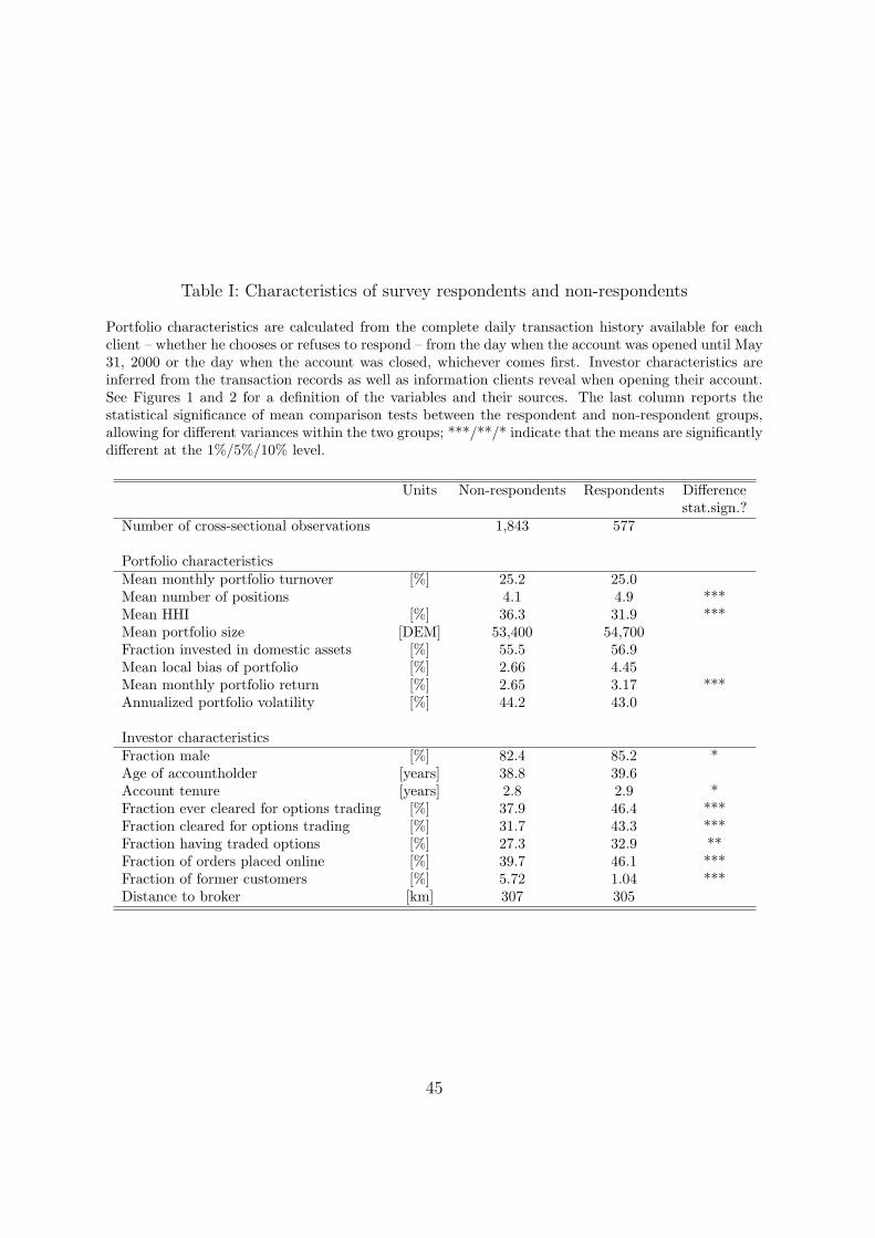
Table I: Characteristics of survey respondents and non-respondents

Portfolio characteristics are calculated from the complete daily transaction history available for eachclient – whether he chooses or refuses to respond – from the day when the account was opened until May31, 2000 or the day when the account was closed, whichever comes first. Investor characteristics areinferred from the transaction records as well as information clients reveal when opening their account.See Figures 1 and 2 for a definition of the variables and their sources. The last column reports thestatistical significance of mean comparison tests between the respondent and non-respondent groups,allowing for different variances within the two groups; ***/**/* indicate that the means are significantlydifferent at the 1%/5%/10% level.

Units Non-respondents Respondents Differencestat.sign.?

Number of cross-sectional observations 1,843 577

Portfolio characteristicsMean monthly portfolio turnover [%] 25.2 25.0Mean number of positions 4.1 4.9 ***Mean HHI [%] 36.3 31.9 ***Mean portfolio size [DEM] 53,400 54,700Fraction invested in domestic assets [%] 55.5 56.9Mean local bias of portfolio [%] 2.66 4.45Mean monthly portfolio return [%] 2.65 3.17 ***Annualized portfolio volatility [%] 44.2 43.0

Investor characteristicsFraction male [%] 82.4 85.2 *Age of accountholder [years] 38.8 39.6Account tenure [years] 2.8 2.9 *Fraction ever cleared for options trading [%] 37.9 46.4 ***Fraction cleared for options trading [%] 31.7 43.3 ***Fraction having traded options [%] 27.3 32.9 **Fraction of orders placed online [%] 39.7 46.1 ***Fraction of former customers [%] 5.72 1.04 ***Distance to broker [km] 307 305

45

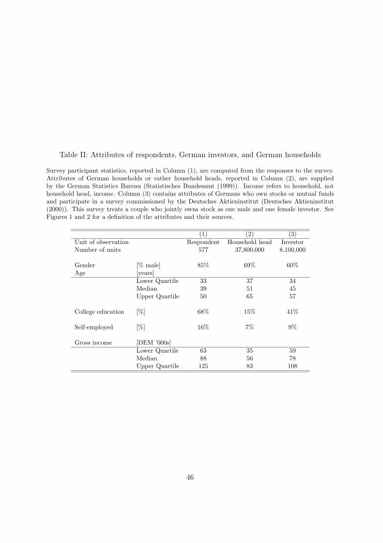
Table II: Attributes of respondents, German investors, and German households

Survey participant statistics, reported in Column (1), are computed from the responses to the survey.Attributes of German households or rather household heads, reported in Column (2), are suppliedby the German Statistics Bureau (Statistisches Bundesamt (1999)). Income refers to household, nothousehold head, income. Column (3) contains attributes of Germans who own stocks or mutual fundsand participate in a survey commissioned by the Deutsches Aktieninstitut (Deutsches Aktieninstitut(2000)). This survey treats a couple who jointly owns stock as one male and one female investor. SeeFigures 1 and 2 for a definition of the attributes and their sources.

(1) (2) (3)Unit of observation Respondent Household head InvestorNumber of units 577 37,800,000 8,100,000

Gender [% male] 85% 69% 60%Age [years]

Lower Quartile 33 37 34Median 39 51 45Upper Quartile 50 65 57

College education [%] 68% 15% 41%

Self-employed [%] 16% 7% 9%

Gross income [DEM ’000s]Lower Quartile 63 35 59Median 88 56 78Upper Quartile 125 83 108

46

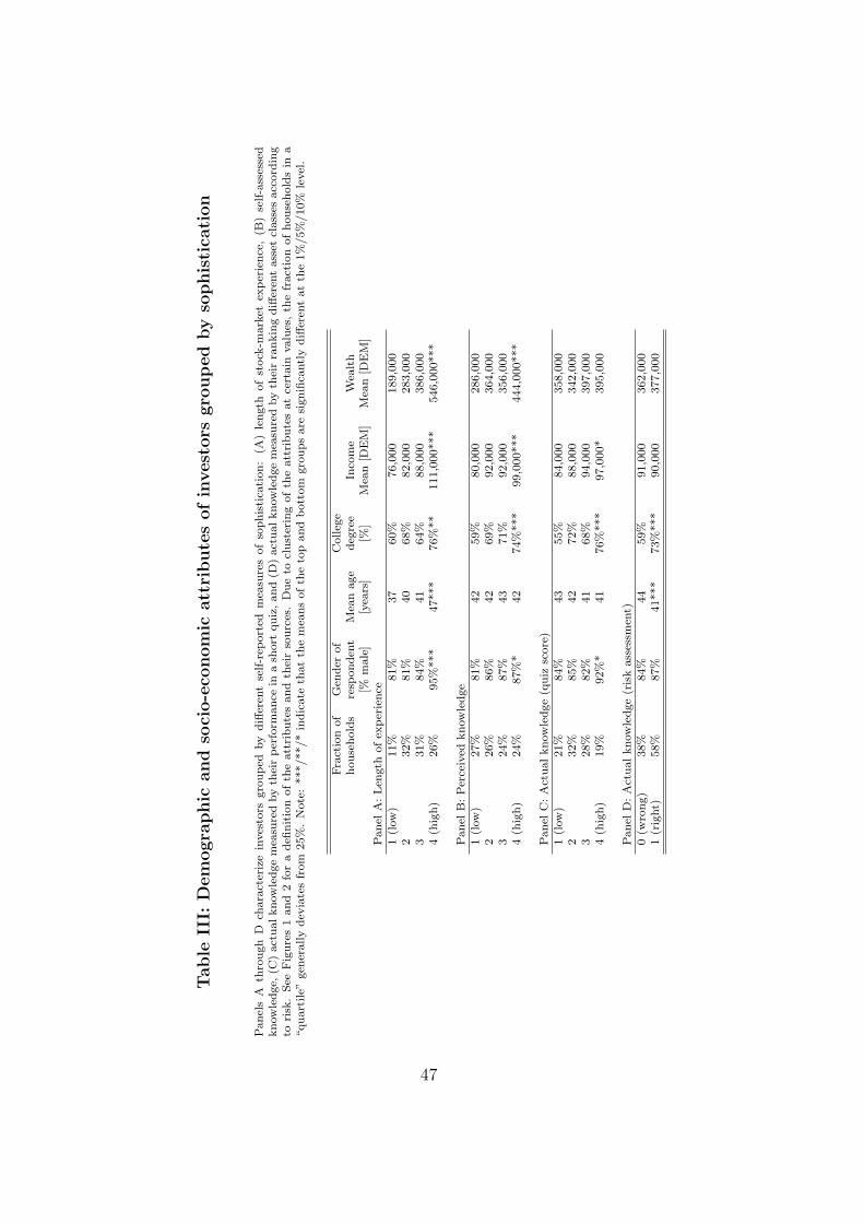
Table

III:

Dem

ogra

phic

and

soci

o-e

conom

icatt

ribute

sofin

vest

ors

gro

uped

by

sophis

tica

tion

Panel

sA

thro

ugh

Dch

ara

cter

ize

inves

tors

gro

uped

by

diff

eren

tse

lf-r

eport

edm

easu

res

of

sophis

tica

tion:

(A)

length

of

stock

-mark

etex

per

ience

,(B

)se

lf-a

sses

sed

know

ledge,

(C)

act

ualknow

ledge

mea

sure

dby

thei

rper

form

ance

ina

short

quiz

,and

(D)

act

ualknow

ledge

mea

sure

dby

thei

rra

nkin

gdiff

eren

tass

etcl

ass

esacc

ord

ing

tori

sk.

See

Fig

ure

s1

and

2fo

ra

defi

nit

ion

ofth

eatt

ribute

sand

thei

rso

urc

es.

Due

tocl

ust

erin

gofth

eatt

ribute

sat

cert

ain

valu

es,th

efr

act

ion

ofhouse

hold

sin

a“quart

ile”

gen

erally

dev

iate

sfr

om

25%

.N

ote

:***/**/*

indic

ate

that

the

mea

ns

ofth

eto

pand

bott

om

gro

ups

are

signifi

cantl

ydiff

eren

tat

the

1%

/5%

/10%

level

.

Fra

ctio

nof

Gen

der

of

Colleg

ehouse

hold

sre

sponden

tM

ean

age

deg

ree

Inco

me

Wea

lth

[%m

ale

][y

ears

][%

]M

ean

[DE

M]

Mea

n[D

EM

]Panel

A:Len

gth

ofex

per

ience

1(l

ow

)11%

81%

37

60%

76,0

00

189,0

00

232%

81%

40

68%

82,0

00

283,0

00

331%

84%

41

64%

88,0

00

386,0

00

4(h

igh)

26%

95%

***

47***

76%

**

111,0

00***

546,0

00***

Panel

B:Per

ceiv

edknow

ledge

1(l

ow

)27%

81%

42

59%

80,0

00

286,0

00

226%

86%

42

69%

92,0

00

364,0

00

324%

87%

43

71%

92,0

00

356,0

00

4(h

igh)

24%

87%

*42

74%

***

99,0

00***

444,0

00***

Panel

C:A

ctualknow

ledge

(quiz

score

)1

(low

)21%

84%

43

55%

84,0

00

358,0

00

232%

85%

42

72%

88,0

00

342,0

00

328%

82%

41

68%

94,0

00

397,0

00

4(h

igh)

19%

92%

*41

76%

***

97,0

00*

395,0

00

Panel

D:A

ctualknow

ledge

(ris

kass

essm

ent)

0(w

rong)

38%

84%

44

59%

91,0

00

362,0

00

1(r

ight)

58%

87%

41***

73%

***

90,0

00

377,0

00

47

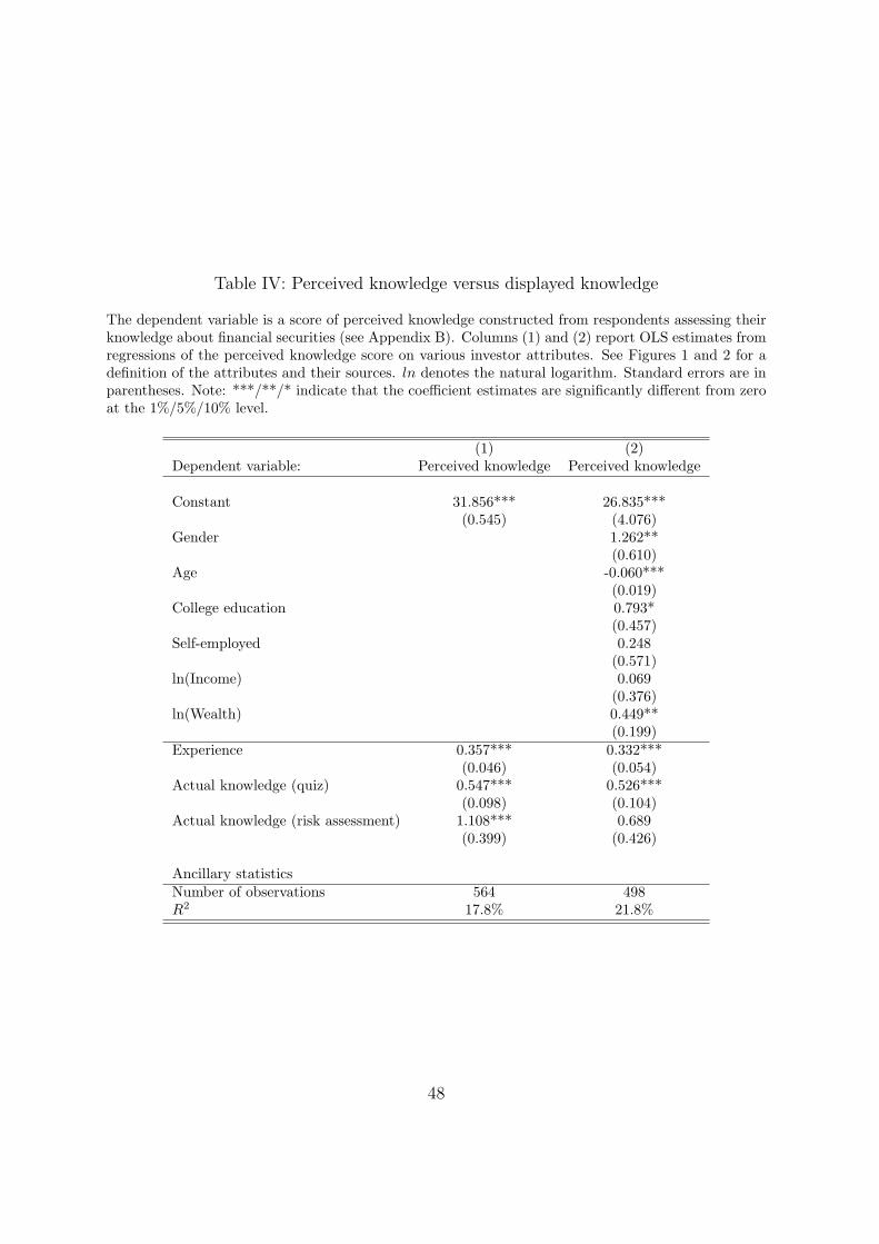
Table IV: Perceived knowledge versus displayed knowledge

The dependent variable is a score of perceived knowledge constructed from respondents assessing theirknowledge about financial securities (see Appendix B). Columns (1) and (2) report OLS estimates fromregressions of the perceived knowledge score on various investor attributes. See Figures 1 and 2 for adefinition of the attributes and their sources. ln denotes the natural logarithm. Standard errors are inparentheses. Note: ***/**/* indicate that the coefficient estimates are significantly different from zeroat the 1%/5%/10% level.

(1) (2)Dependent variable: Perceived knowledge Perceived knowledge

Constant 31.856*** 26.835***(0.545) (4.076)

Gender 1.262**(0.610)

Age -0.060***(0.019)

College education 0.793*(0.457)

Self-employed 0.248(0.571)

ln(Income) 0.069(0.376)

ln(Wealth) 0.449**(0.199)

Experience 0.357*** 0.332***(0.046) (0.054)

Actual knowledge (quiz) 0.547*** 0.526***(0.098) (0.104)

Actual knowledge (risk assessment) 1.108*** 0.689(0.399) (0.426)

Ancillary statisticsNumber of observations 564 498R2 17.8% 21.8%

48

Table V: The relation between overconfidence and other investor attributes

Columns (1) and (2) report the estimates from ordered probit regressions of the self-attribution biasscore and the control score on various investor attributes. See Figures 1 and 2 for a definition of theattributes and their sources. ln denotes the natural logarithm. Standard errors are in parentheses. Note:***/**/* indicate that the coefficient estimates are significantly different from zero at the 1%/5%/10%level.

(1) (2)Dependent variable: Self-attribution bias Control score

Gender -0.086 -0.052(0.139) (0.138)

Age 0.007 -0.009**(0.004) (0.004)

College education -0.065 -0.065(0.104) (0.103)

Self-employed 0.070 -0.068(0.130) (0.128)

ln(Income) 0.009 -0.007(0.085) (0.084)

ln(Wealth) 0.003 0.031(0.045) (0.045)

Experience 0.011 0.022*(0.013) (0.013)

Actual knowledge (quiz) -0.035 0.005(0.024) (0.024)

Actual knowledge (risk assessment) 0.021 0.170*(0.097) (0.096)

Perceived knowledge -0.010 0.037***(0.010) (0.010)

Ancillary statisticsNumber of observations 495 498Pseudo R2 0.6% 1.5%

49

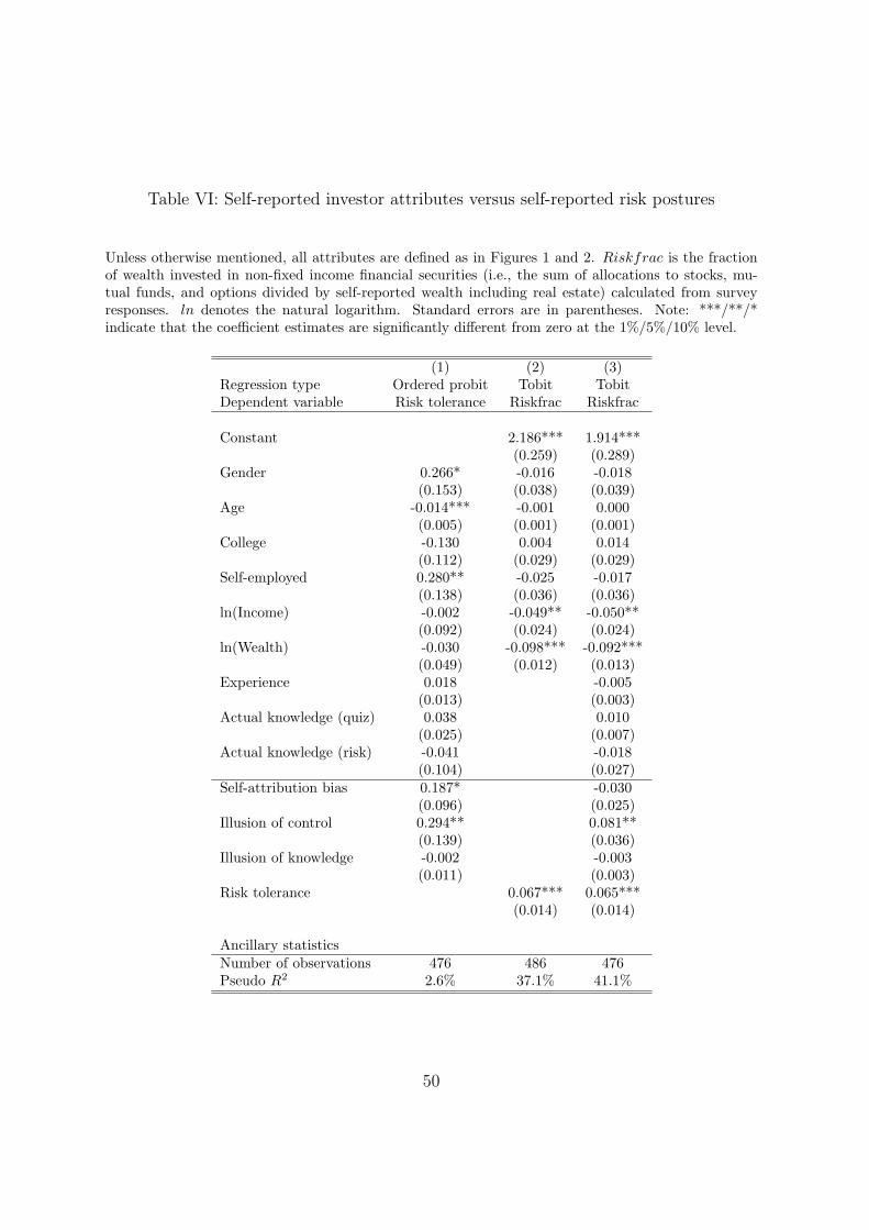
Table VI: Self-reported investor attributes versus self-reported risk postures

Unless otherwise mentioned, all attributes are defined as in Figures 1 and 2. Riskfrac is the fractionof wealth invested in non-fixed income financial securities (i.e., the sum of allocations to stocks, mu-tual funds, and options divided by self-reported wealth including real estate) calculated from surveyresponses. ln denotes the natural logarithm. Standard errors are in parentheses. Note: ***/**/*indicate that the coefficient estimates are significantly different from zero at the 1%/5%/10% level.

(1) (2) (3)Regression type Ordered probit Tobit TobitDependent variable Risk tolerance Riskfrac Riskfrac

Constant 2.186*** 1.914***(0.259) (0.289)

Gender 0.266* -0.016 -0.018(0.153) (0.038) (0.039)

Age -0.014*** -0.001 0.000(0.005) (0.001) (0.001)

College -0.130 0.004 0.014(0.112) (0.029) (0.029)

Self-employed 0.280** -0.025 -0.017(0.138) (0.036) (0.036)

ln(Income) -0.002 -0.049** -0.050**(0.092) (0.024) (0.024)

ln(Wealth) -0.030 -0.098*** -0.092***(0.049) (0.012) (0.013)

Experience 0.018 -0.005(0.013) (0.003)

Actual knowledge (quiz) 0.038 0.010(0.025) (0.007)

Actual knowledge (risk) -0.041 -0.018(0.104) (0.027)

Self-attribution bias 0.187* -0.030(0.096) (0.025)

Illusion of control 0.294** 0.081**(0.139) (0.036)

Illusion of knowledge -0.002 -0.003(0.011) (0.003)

Risk tolerance 0.067*** 0.065***(0.014) (0.014)

Ancillary statisticsNumber of observations 476 486 476Pseudo R2 2.6% 37.1% 41.1%

50

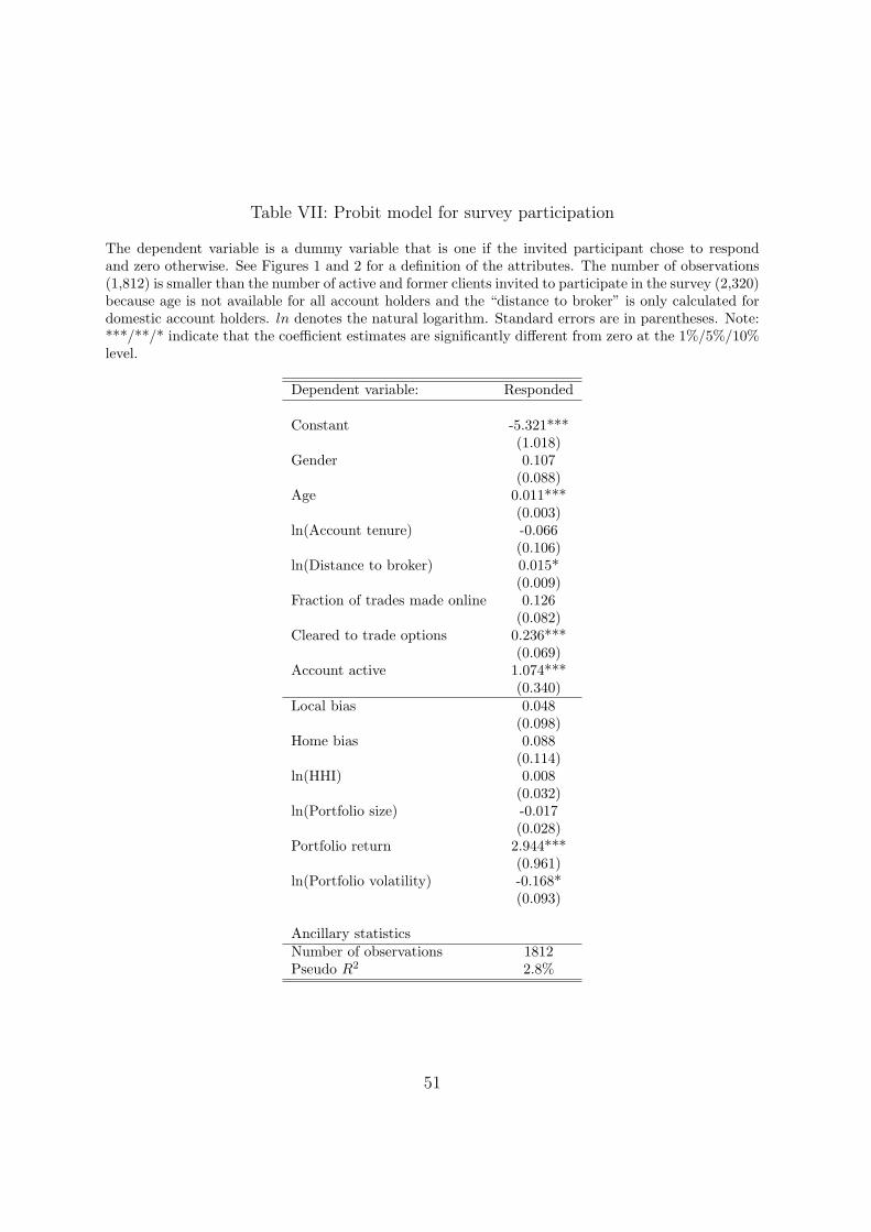
Table VII: Probit model for survey participation

The dependent variable is a dummy variable that is one if the invited participant chose to respondand zero otherwise. See Figures 1 and 2 for a definition of the attributes. The number of observations(1,812) is smaller than the number of active and former clients invited to participate in the survey (2,320)because age is not available for all account holders and the “distance to broker” is only calculated fordomestic account holders. ln denotes the natural logarithm. Standard errors are in parentheses. Note:***/**/* indicate that the coefficient estimates are significantly different from zero at the 1%/5%/10%level.

Dependent variable: Responded

Constant -5.321***(1.018)

Gender 0.107(0.088)

Age 0.011***(0.003)

ln(Account tenure) -0.066(0.106)

ln(Distance to broker) 0.015*(0.009)

Fraction of trades made online 0.126(0.082)

Cleared to trade options 0.236***(0.069)

Account active 1.074***(0.340)

Local bias 0.048(0.098)

Home bias 0.088(0.114)

ln(HHI) 0.008(0.032)

ln(Portfolio size) -0.017(0.028)

Portfolio return 2.944***(0.961)

ln(Portfolio volatility) -0.168*(0.093)

Ancillary statisticsNumber of observations 1812Pseudo R2 2.8%

51

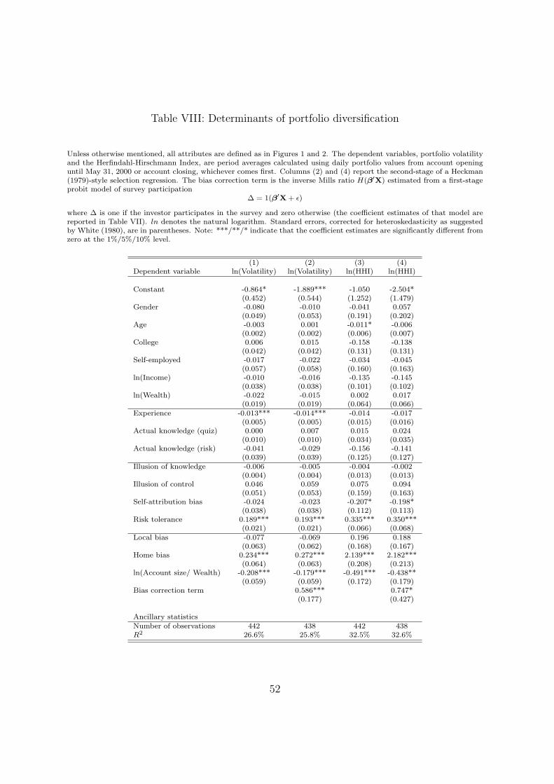
Table VIII: Determinants of portfolio diversification

Unless otherwise mentioned, all attributes are defined as in Figures 1 and 2. The dependent variables, portfolio volatilityand the Herfindahl-Hirschmann Index, are period averages calculated using daily portfolio values from account openinguntil May 31, 2000 or account closing, whichever comes first. Columns (2) and (4) report the second-stage of a Heckman(1979)-style selection regression. The bias correction term is the inverse Mills ratio H(β′X) estimated from a first-stageprobit model of survey participation

∆ = 1(β′X + ε)

where ∆ is one if the investor participates in the survey and zero otherwise (the coefficient estimates of that model arereported in Table VII). ln denotes the natural logarithm. Standard errors, corrected for heteroskedasticity as suggestedby White (1980), are in parentheses. Note: ***/**/* indicate that the coefficient estimates are significantly different fromzero at the 1%/5%/10% level.

(1) (2) (3) (4)Dependent variable ln(Volatility) ln(Volatility) ln(HHI) ln(HHI)

Constant -0.864* -1.889*** -1.050 -2.504*(0.452) (0.544) (1.252) (1.479)

Gender -0.080 -0.010 -0.041 0.057(0.049) (0.053) (0.191) (0.202)

Age -0.003 0.001 -0.011* -0.006(0.002) (0.002) (0.006) (0.007)

College 0.006 0.015 -0.158 -0.138(0.042) (0.042) (0.131) (0.131)

Self-employed -0.017 -0.022 -0.034 -0.045(0.057) (0.058) (0.160) (0.163)

ln(Income) -0.010 -0.016 -0.135 -0.145(0.038) (0.038) (0.101) (0.102)

ln(Wealth) -0.022 -0.015 0.002 0.017(0.019) (0.019) (0.064) (0.066)

Experience -0.013*** -0.014*** -0.014 -0.017(0.005) (0.005) (0.015) (0.016)

Actual knowledge (quiz) 0.000 0.007 0.015 0.024(0.010) (0.010) (0.034) (0.035)

Actual knowledge (risk) -0.041 -0.029 -0.156 -0.141(0.039) (0.039) (0.125) (0.127)

Illusion of knowledge -0.006 -0.005 -0.004 -0.002(0.004) (0.004) (0.013) (0.013)

Illusion of control 0.046 0.059 0.075 0.094(0.051) (0.053) (0.159) (0.163)

Self-attribution bias -0.024 -0.023 -0.207* -0.198*(0.038) (0.038) (0.112) (0.113)

Risk tolerance 0.189*** 0.193*** 0.335*** 0.350***(0.021) (0.021) (0.066) (0.068)

Local bias -0.077 -0.069 0.196 0.188(0.063) (0.062) (0.168) (0.167)

Home bias 0.234*** 0.272*** 2.139*** 2.182***(0.064) (0.063) (0.208) (0.213)

ln(Account size/ Wealth) -0.208*** -0.179*** -0.491*** -0.438**(0.059) (0.059) (0.172) (0.179)

Bias correction term 0.586*** 0.747*(0.177) (0.427)

Ancillary statisticsNumber of observations 442 438 442 438R2 26.6% 25.8% 32.5% 32.6%

52

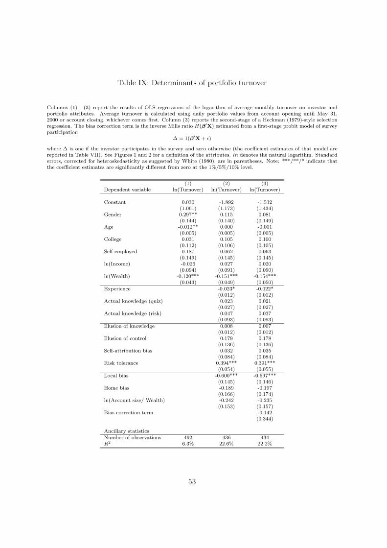
Table IX: Determinants of portfolio turnover

Columns (1) - (3) report the results of OLS regressions of the logarithm of average monthly turnover on investor andportfolio attributes. Average turnover is calculated using daily portfolio values from account opening until May 31,2000 or account closing, whichever comes first. Column (3) reports the second-stage of a Heckman (1979)-style selectionregression. The bias correction term is the inverse Mills ratio H(β′X) estimated from a first-stage probit model of surveyparticipation

∆ = 1(β′X + ε)

where ∆ is one if the investor participates in the survey and zero otherwise (the coefficient estimates of that model arereported in Table VII). See Figures 1 and 2 for a definition of the attributes. ln denotes the natural logarithm. Standarderrors, corrected for heteroskedasticity as suggested by White (1980), are in parentheses. Note: ***/**/* indicate thatthe coefficient estimates are significantly different from zero at the 1%/5%/10% level.

(1) (2) (3)Dependent variable ln(Turnover) ln(Turnover) ln(Turnover)

Constant 0.030 -1.892 -1.532(1.061) (1.173) (1.434)

Gender 0.297** 0.115 0.081(0.144) (0.140) (0.149)

Age -0.012** 0.000 -0.001(0.005) (0.005) (0.005)

College 0.031 0.105 0.100(0.112) (0.106) (0.105)

Self-employed 0.187 0.062 0.063(0.149) (0.145) (0.145)

ln(Income) -0.026 0.027 0.020(0.094) (0.091) (0.090)

ln(Wealth) -0.120*** -0.151*** -0.154***(0.043) (0.049) (0.050)

Experience -0.023* -0.022*(0.012) (0.012)

Actual knowledge (quiz) 0.023 0.021(0.027) (0.027)

Actual knowledge (risk) 0.047 0.037(0.093) (0.093)

Illusion of knowledge 0.008 0.007(0.012) (0.012)

Illusion of control 0.179 0.178(0.136) (0.136)

Self-attribution bias 0.032 0.035(0.084) (0.084)

Risk tolerance 0.394*** 0.391***(0.054) (0.055)

Local bias -0.600*** -0.597***(0.145) (0.146)

Home bias -0.189 -0.197(0.166) (0.174)

ln(Account size/ Wealth) -0.242 -0.235(0.153) (0.157)

Bias correction term -0.142(0.344)

Ancillary statisticsNumber of observations 492 436 434R2 6.3% 22.6% 22.2%

53