Talbot images of wavelength-scale amplitude gratings images of... · Talbot images of wavelength-scale amplitude gratings ... L. M. Sanchez-Brea, and J. Vargas, ... (Roberts & Company,

Talbot images of wavelength-scale amplitude gratings

Myun-Sik Kim,1,*

Toralf Scharf,1 Christoph Menzel,

2 Carsten Rockstuhl,

2

and Hans Peter Herzig1

1Optics & Photonics Technology Laboratory, Ecole Polytechnique Fédérale de Lausanne (EPFL), Neuchâtel, CH-2000, Switzerland

2Institute of Condensed Matter Theory and Solid State Optics, Abbe Center of Photonics, Friedrich-Schiller-Universität Jena, 07743 Jena, Germany

*[email protected]

Abstract: By means of experiment and simulation, we achieve unprecedented insights into the formation of Talbot images to be observed in transmission for light diffracted at wavelength-scale amplitude gratings. Emphasis is put on disclosing the impact and the interplay of various diffraction orders to the formation of Talbot images. They can be manipulated by selective filtering in the Fourier plane. Experiments are performed with a high-resolution interference microscope that measures the amplitude and phase of fields in real-space. Simulations have been performed using rigorous diffraction theory. Specific phase features, such as singularities found in the Talbot images, are discussed. This detailed analysis helps to understand the response of fine gratings. It provides moreover new insights into the fundamental properties of gratings that often find use in applications such as, e.g., lithography, sensing, and imaging.

©2012 Optical Society of America

OCIS codes: (050.1950) Diffraction gratings; (050.1960) Diffraction theory; (070.6760) Talbot and self-imaging effects; (070.0070) Fourier optics and signal processing; (070.6110) Spatial filtering; (180.3170) Interference microscopy.

References and links

1. F. Talbot, “Facts relating to optical science. No. IV,” Philos. Mag. 9, 401–407 (1836). 2. L. Rayleigh, “On copying diffraction gratings and some phenomena connected therewith,” Philos. Mag. 11, 196–

205 (1881). 3. R. F. Edgar, “The Fresnel diffraction images of periodic structures,” J. Mod. Opt. 16, 281–287 (1969). 4. J. T. Winthrop and C. R. Worthington, “Theory of Fresnel images. I. Plane periodic objects in monochromatic

light,” J. Opt. Soc. Am. 55(4), 373–381 (1965). 5. A. Kołodziejczyk, “Realization of Fourier images without using a lens by sampling the optical object,” J. Mod.

Opt. 32, 74–746 (1985). 6. Y.-S. Cheng and R.-C. Chang, “Theory of image formation using the Talbot effect,” Appl. Opt. 33(10), 1863–

1874 (1994). 7. S. Teng, Y. Tan, and C. Cheng, “Quasi-Talbot effect of the high-density grating in near field,” J. Opt. Soc. Am.

A 25(12), 2945–2951 (2008). 8. M. Berry and S. Klein, “Integer, fractional and fractal Talbot effects,” J. Mod. Opt. 43(10), 2139–2164 (1996). 9. E. Noponen and J. Turunen, “Electromagnetic theory of Talbot imaging,” Opt. Commun. 98(1-3), 132–140

(1993). 10. Y. Lu, C. Zhou, and H. Luo, “Talbot effect of a grating with different kinds of flaws,” J. Opt. Soc. Am. A 22(12),

2662–2667 (2005). 11. F. J. Torcal-Milla, L. M. Sanchez-Brea, and J. Vargas, “Effect of aberrations on the self-imaging phenomenon,”

J. Lightwave Technol. 29(7), 1051–1057 (2011). 12. O. Bryngdahl, “Image formation using self-imaging techniques,” J. Opt. Soc. Am. 63(4), 416–419 (1973). 13. J. C. Bhattacharya, “Measurement of the refractive index using the Talbot effect and a moire technique,” Appl.

Opt. 28(13), 2600–2604 (1989). 14. G. Spagnolo, D. Ambrosini, and D. Paoletti, “Displacement measurement using the Talbot effect with a Ronchi

grating,” J. Opt. A: Pure Appl. Opt 4(6), S376–S380 (2002). 15. A. Isoyan, F. Jiang, Y. C. Cheng, F. Cerrina, P. Wachulak, L. Urbanski, J. Rocca, C. Menoni, and M. Marconi,

“Talbot lithography: self-imaging of complex structures,” J. Vac. Sci. Technol. B 27(6), 2931–2937 (2009).

#160032 - $15.00 USD Received 14 Dec 2011; revised 3 Feb 2012; accepted 3 Feb 2012; published 13 Feb 2012(C) 2012 OSA 27 February 2012 / Vol. 20, No. 5 / OPTICS EXPRESS 4903

16. L. Stuerzebecher, T. Harzendorf, U. Vogler, U. D. Zeitner, and R. Voelkel, “Advanced mask aligner lithography: fabrication of periodic patterns using pinhole array mask and Talbot effect,” Opt. Express 18(19), 19485–19494 (2010).

17. A. W. Lohmann and J. A. Thomas, “Making an array illuminator based on the talbot effect,” Appl. Opt. 29(29), 4337–4340 (1990).

18. F. Huang, N. Zheludev, Y. Chen, and F. de Abajo, “Focusing of light by a nanohole array,” Appl. Phys. Lett. 90(9), 091119 (2007).

19. M. Berry, I. Marzoli, and W. Schleich, “Quantum carpets, carpets of light,” Phys. World 39–46 (June 2001) 20. X.-B. Song, H.-B. Wang, J. Xiong, K. Wang, X. Zhang, K.-H. Luo, and L.-A. Wu, “Experimental observation of

quantum Talbot effects,” Phys. Rev. Lett. 107(3), 033902 (2011). 21. M. S. Chapman, C. R. Ekstrom, T. D. Hammond, J. Schmiedmayer, B. E. Tannian, S. Wehinger, and D. E.

Pritchard, “Near-field imaging of atom diffraction gratings: The atomic Talbot effect,” Phys. Rev. A 51(1), R14–R17 (1995).

22. S. Nowak, Ch. Kurtsiefer, T. Pfau, and C. David, “High-order Talbot fringes for atomic matter waves,” Opt. Lett. 22(18), 1430–1432 (1997).

23. P. Cloetens, J. P. Guigay, C. De Martino, J. Baruchel, and M. Schlenker, “Fractional Talbot imaging of phase gratings with hard x rays,” Opt. Lett. 22(14), 1059–1061 (1997).

24. B. J. McMorran and A. D. Cronin, “An electron Talbot interferometer,” New J. Phys. 11(3), 033021 (2009). 25. M. R. Dennis, N. I. Zheludev, and F. J. García de Abajo, “The plasmon Talbot effect,” Opt. Express 15(15),

9692–9700 (2007). 26. S. Cherukulappurath, D. Heinis, J. Cesario, N. F. van Hulst, S. Enoch, and R. Quidant, “Local observation of

plasmon focusingin Talbot carpets,” Opt. Express 17(26), 23772–23784 (2009). 27. A. Nesci, R. Dändliker, M. Salt, and H. P. Herzig, “Measuring amplitude and phase distribution of fields

generated by gratings with sub-wavelength resolution,” Opt. Commun. 205(4-6), 229–238 (2002). 28. D. Goldstein, Understanding the Light Microscope: A Computer-Aided Introduction (Academic Press, 1999),

Chap. 1. 29. D. Malacara, Optical Shop Testing (Wiley, 2007), 3rd ed., Chap. 16. 30. M.-S. Kim, T. Scharf, and H. P. Herzig, “Amplitude and phase measurements of highly focused light in optical

data storage systems,” Jpn. J. Appl. Phys. 49(8), 08KA03 (2010). 31. M.-S. Kim, T. Scharf, and H. P. Herzig, “Small-size microlens characterization by multiwavelength high-

resolution interference microscopy,” Opt. Express 18(14), 14319–14329 (2010). 32. M.-S. Kim, T. Scharf, S. Mühlig, C. Rockstuhl, and H. P. Herzig, “Engineering photonic nanojets,” Opt. Express

19(11), 10206–10220 (2011). 33. M.-S. Kim, T. Scharf, M. T. Haq, W. Nakagawa, and H. P. Herzig, “Subwavelength-size solid immersion lens,”

Opt. Lett. 36(19), 3930–3932 (2011). 34. C. Rockstuhl, I. Märki, T. Scharf, M. Salt, H. P. Herzig, and R. Dändliker, “High resolution interference

microscopy: a tool for probing optical waves in the far-field on a nanometric length scale,” Curr. Nanosci. 2(4), 337–350 (2006).

35. J. Schwider, R. Burow, K.-E. Elssner, J. Grzanna, R. Spolaczyk, and K. Merkel, “Digital wave-front measuring interferometry: some systematic error sources,” Appl. Opt. 22(21), 3421–3432 (1983).

36. P. Hariharan, B. F. Oreb, and T. Eiju, “Digital phase-shifting interferometry: a simple error-compensating phase calculation algorithm,” Appl. Opt. 26(13), 2504–2506 (1987).

37. M. Born and E. Wolf, Principles of Optics, 7th ed. (Cambridge University Press, 1999). 38. E. Abbe, “Beiträge zur theorie des mikroskops und der mikroskopischen wahrnehmung,” Arch. Mikrosc. Anat.

Entwicklungsmech 9(1), 413–418 (1873). 39. H. Köhler, “On Abbe’s theory of image formation in the microscope,” Opt. Acta (Lond.) 28(12), 1691–1701

(1981). 40. H. Gross, H. Zugge, M. Peschka, and F. Blechinger, Handbook of Optical Systems (Wiley, 2007), Vol. 3, p. 126. 41. J. W. Goodman, Introduction to Fourier Optics, 3rd ed. (Roberts & Company, 2005), Chap. 6. 42. H. Gundlach, “From the history of microscopy: Abbe’s diffraction trials,” Innovation, The Magazine from Carl

Zeiss 15, 18–23 (2005). 43. L. Li, “New formulation of the Fourier modal method for crossed surface-relief gratings,” J. Opt. Soc. Am. A

14(10), 2758–2767 (1997). 44. T. Paul, C. Rockstuhl, and F. Lederer, “Integrating cold plasma equations into the Fourier modal method to

analyze second harmonic generation at metallic nanostructures,” J. Mod. Opt. 58(5-6), 438–448 (2011). 45. E. P. Goodwin and J. C. Wyant, Field Guide to Interferometric Optical Testing (SPIE, 2006). 46. S. Yokozeki, “Moiré fringes,” Opt. Lasers Eng. 3(1), 15–27 (1982). 47. N. W. Ashcroft and N. D. Mermin, Solid State Physics (Saunders College Publishing, 1976), Chap. 6. 48. R. G. Griggers, Encyclopedia of Optical Engineering (CRC Press, 2003), p. 1928.

1. Introduction

Periodic structures diffract light, and such diffracted light interferes in the vicinity of the structure. Potentially the simplest example for a periodic structure is an amplitude grating that diffracts the light into discrete directions. In the Fresnel diffraction regime, these diffraction orders interfere and cause a self-imaging phenomenon of the grating. This phenomenon is known as the Talbot effect, named in honor of his discovery by F. Talbot in 1836 [1]. The


Talbot effect says that the field behind the grating possesses a periodicity in axial direction, in addition to the periodicity in lateral directions due to the periodicity of the object. The field distribution repeats at regular distances away from the grating surface. This regular distance was derived within the paraxial approximation by Lord Rayleigh in 1881 and was called the Talbot length [2].

The Talbot effect has been intensively studied both theoretically and experimentally. The theoretical studies often focused on a discussion of the origin of the Talbot effect and associated phenomena. Different phenomena and their origins were discussed while imposing different approximations. Work has been done in the framework of Fresnel diffraction [3], Fresnel images [4], Fourier images [5], theory of image formation [6], and effects such as the quasi-Talbot effect [7] or the fractional and fractal Talbot effects [8] were investigated. Also, rigorous studies were done using, e.g., electromagnetic theory [9], the finite-difference time-domain (FDTD) method [10] and the Rayleigh-Sommerfeld formula for effects of aberrations on the self-imaging process [11]. There are much less experimental investigations documented. The majority concentrated on proposing applications that exploit the Talbot effect, for example, for imaging [12], measuring the refractive index [13], sensing a distance and a displacement [14], lithography [15, 16], array illumination [17], and sub-wavelength focusing [18]. In physical optics, researchers discussed effects down to the quantum mechanics level, i.e. the quantum Talbot effect [19, 20]. Such self-imaging phenomena are not only limited to the optical spectrum. Talbot effect exits for atomic matter waves [21, 22], x-ray [23], electron beams [24], and surface plasmons [25,26].

In all such studies, the contribution of each diffraction order to the Talbot effect, to the best of our knowledge, has never been discussed on experimental grounds. Moreover, a typical Talbot experiment relies on gratings with periods that are large compared to the wavelength. The diffraction formula for the grating at normal incidence is given as

sin ,m

mλθ =

Λ (1)

where θ is the diffraction angle, m is the diffraction order, and Λ is the period of a grating. The small-angle approximation finally leads to Eq. (1) sinθ ~θ, when λ/Λ is small; usually called the paraxial approximation [2, 19]. Such an approximation makes the experimental and theoretical conditions easier and simpler to control; but the number of diffraction orders that contribute the formation of an image is huge. In consequence, the individual manipulation of an individual diffraction order and the discussion of its impact turn out to be a tedious task. Therefore, gratings with a smaller period are much more appealing to discuss the impact of individual diffraction orders to the formation of the Talbot images.

In the past, scanning near-field optical microscopy (SNOM) was used to measure the amplitude and phase distributions emerging from a 1-µm-period grating [27]. Although SNOM assures an increased spatial resolution due to its capability to resolve truly subwavelength features, the unavoidable scanning in the axial direction renders the experimental efforts complicated and the manipulation of diffraction orders in a Fourier plane is also not possible.

In this paper, we experimentally study the diffraction of light by wavelength-scale-period gratings in the Fresnel diffraction regime with a high-resolution interference microscope (HRIM). Note that the Fresnel diffraction regime stands for the measurement space close to the grating surface, not for the Fresnel approximations. The HRIM allows to record three-dimensional (3D) amplitude and phase fields of light in real space emerging from the grating in transmission. The space can be immersed in air, water, or index matching oil and the use of high numerical aperture (NA) objectives allows to collect a large number of diffraction orders. Unique to our experimental approach is the possibility to manipulate the Fourier plane of the observing objective lens by a Bertrand lens [28]. It allows us to select specific diffraction orders. The Talbot images are called throughout the manuscript as artificial Talbot images, when some diffraction orders are filtered. We discuss the influence of wavelengths,


the refractive index of the immersion medium and the number of diffraction orders on the Talbot images, which are recorded as amplitude and phase fields. Since the gratings have critical dimensions in the order of the wavelength, their optical action cannot be described while imposing approximations to Maxwell’s equations, i.e. the thin-element approximation. Therefore, rigorous numerical means are used to solve Maxwell’s equations, taking into account all miniscule details of the experiment. This approach allows to support entirely all our experimental results.

We will discuss in detail experimental and numerical results with one-dimensional (1D) amplitude gratings with periods of 1 µm and 2 µm with the filling ratio 0.5 defined as d/Λ, where d is the width, which the grating material occupies within the period. They are fabricated on a glass substrate by depositing gold with a thickness of 150 nm. The polarization effect has been considered, but there was practically no influence, since no polarization sensitive resonance is evoked in the interaction process. Therefore, most of the results we present are for an illumination with a plane wave propagating along the positive z-direction and being polarized in the x-direction, which is the TM case for the grating.

1.1 Talbot length

In 1881, Lord Rayleigh showed that the origin of the repeated intensity modulation in the propagation direction after periodic structures, the Talbot effect, is a result of interferences of diffracted beams and found the characteristic Talbot length ZT [2] to be

2

.

1 1

TZλ

λ=

− −

Λ

(2)

He also suggested the simplification of Eq. (2) when the wavelengths λ is considered to be small compared to the period Λ of the structure. In this paraxial approximation the Talbot length can be expressed by

2

2.

TZ

λ

Λ= (3)

Surprisingly, this simplified formula [Eq. (3)] is still sufficiently accurate for fine-period gratings, whose period becomes comparable to the wavelength. For instance, the difference between the Talbot lengths, which is calculated by Eqs. (2) and (3) for a grating of 1.5λ period at 642-nm wavelength, is smaller than 400 nm. This is often negligible in experiments because the axial resolution of the far-field measurement system is in general larger than this value. Although for our wavelength-scale-period gratings the paraxial approximation cannot be considered anymore as valid, i.e., λ/Λ is not small anymore, Eq. (3) is still suitable for anticipating the Talbot length and verifying experimental results for such fine-period gratings.

1.2 Sub-images by quasi- and fractional-Talbot effect

Apart from the self-images, which occur at multiples of half the Talbot length with a lateral period identical to the period of the grating, sub-images also exist at smaller fractions of the Talbot length (i.e. the sub-Talbot planes). The field in these sub-images possesses a smaller lateral period when compared to that of the self-images [7, 8]. For example, gratings with a relatively large period compared to the illuminating wavelength generate a large number of diffraction orders. When the higher diffraction orders can destructively interfere with the lower orders, sub-images with smaller fractions of the original lateral periodicity appear in the sub-Talbot planes. The influence and role of the higher diffraction orders will be discussed in section 4 by filtering lower diffraction orders.


2. Experimental setup

2.1 High-resolution interference microscope

High-resolution interference microscopy is a holographic microscopy in a sense that it records interferograms of an object with a reference field. By measuring multiple interferograms with an adjustable phase difference between object and reference field, the amplitude and phase distributions of the object field can be retrieved. In general, interferometric testing systems have been developed for two-dimensional (2D) measurements, for example, surface profiling and wavefront measurements of light fields in a plane of interest [29]. The major difference of our HRIM when compared to other interference microscopes is the ability to record amplitude and phase fields in 3D by scanning the samples along the axial direction and repeating the measurement procedure. Furthermore, the HRIM is reinforced with auxiliary techniques known from conventional microscopy, which are often difficult to be implemented in other types of holographic or interferometric microscopes.

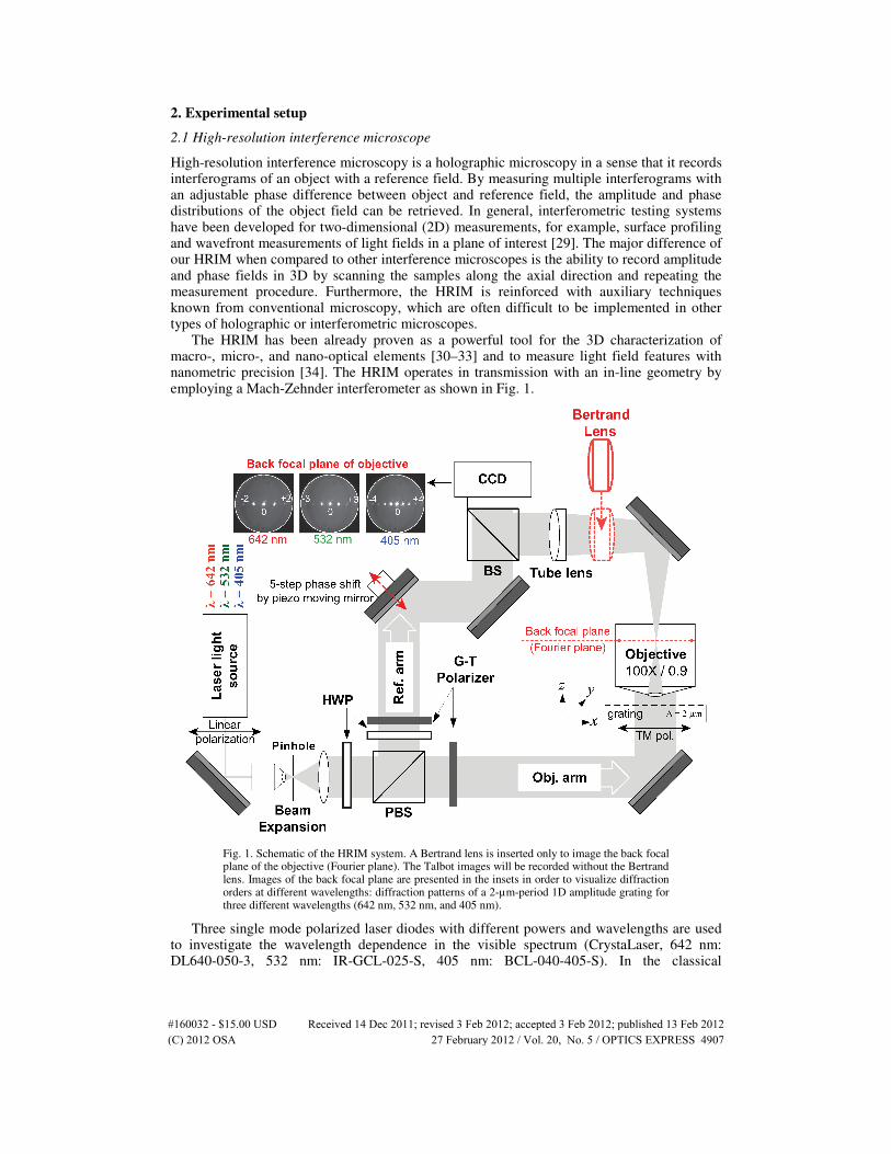
The HRIM has been already proven as a powerful tool for the 3D characterization of macro-, micro-, and nano-optical elements [30–33] and to measure light field features with nanometric precision [34]. The HRIM operates in transmission with an in-line geometry by employing a Mach-Zehnder interferometer as shown in Fig. 1.

Fig. 1. Schematic of the HRIM system. A Bertrand lens is inserted only to image the back focal plane of the objective (Fourier plane). The Talbot images will be recorded without the Bertrand lens. Images of the back focal plane are presented in the insets in order to visualize diffraction orders at different wavelengths: diffraction patterns of a 2-µm-period 1D amplitude grating for three different wavelengths (642 nm, 532 nm, and 405 nm).

Three single mode polarized laser diodes with different powers and wavelengths are used to investigate the wavelength dependence in the visible spectrum (CrystaLaser, 642 nm: DL640-050-3, 532 nm: IR-GCL-025-S, 405 nm: BCL-040-405-S). In the classical


interferometric arrangement a polarizing beam splitter (PBS) divides the incident light in a reference and an object arm with adjustable energy ratio. Half wave plates (HWP) and Glan-Taylor (G-T) polarizers are used to adjust the intensities and to optimize the contrast of the interference fringes. In the reference arm, a piezo-electrically driven mirror is mounted to change the optical path length. The phase distribution of the wave field is obtained by measuring the interference fringes at different mirror positions and employing the well-known 5-frame algorithm, which is called Schwider-Hariharan method [35, 36]. Five frames of the intensity pattern, from which the 2D phase information can be directly retrieved, are recorded with each frame being shifted by adding an optical path of λ/4 or 0.5π. The grating sample is mounted on a precision piezo stage with a z-scan range of 500 µm and a nominal accuracy of 1 nm (MAD LAB CITY, NANO Z500). This z-axis piezo stage is used to precisely define the plane of interest at the highest resolution and measure 3D light fields emerging from the wavelength-scale gratings by scanning the grating along the axial direction.

In general, a high numerical aperture (NA) of the observation objective ensures high-resolution of the amplitude and phase measurements. Moreover, high magnification leads to more pixels per area on an image sensor for small fields. While not really useful if intensity only fields are recorded, the phase imaging profits from such oversampling because features of the phase field are not subject to the resolution limit [34]. The resolving power for intensity features, i.e., the resolution of an optical imaging system like a microscope, can be limited by factors such as imperfections of the lenses or misalignment. However, there is also a more fundamental limit to the resolution of any optical system which is due to diffraction. An optical system with the ability to produce images with angular resolution as good as the instrument's theoretical limit is said to be diffraction limited [37]. Assuming that optical aberrations in the whole optical setup are negligible, the lateral resolution d can be stated as the Abbe limit (∆x) = λ / 2NA [38, 39], which has been named in honor of Ernst K. Abbe. For example, the nominal lateral resolutions for a 100X / NA 0.9 objective (Leica Microsystems, HC PL FLUOTAR) equipped in the HRIM is calculated to be 357 nm at a wavelength of 642 nm. Along the optical axis, the Rayleigh criterion can be applied with the simplified formula derived as ∆z = λ·n / (NA

2), where n is the refractive index of the medium [40]. The calculated

axial resolution at a wavelength of 642 nm is ∆z = 793 nm. At 100X magnification, a pixel on our charge-coupled device (CCD) sensor (Sicon Corporation, CFW1312M camera with SONY ICX205AK image sensor of 1360 x 1024 pixels) corresponds to 46.5 nm in the object plane. This leads to the maximum field of view of the CCD camera of 64 x 48 µm

2, which is

sufficiently large to investigate small-period gratings.

2.2 Spatial filtering at the Fourier plane

Spatial filtering and the Fourier plane manipulation play an important role not only in image processing but also in understanding fundamental principles in optics. Abbe pioneered the manipulation of the Fourier plane in order to investigate the image formation of microscopy [41]. He created various diffraction experiments and tried to monitor and manipulate light in the back focal plane of the objective. Removal of the eyepiece and the use of an auxiliary lens permitted him the observation of the back focal plane. By such experiments with a series of diffraction gratings, he succeeded in deriving the theory of image formation and the resolution limit of microscopy [39, 42]. When diffraction elements, such as diffraction gratings, are under investigation, monitoring the Fourier plane and filtering some diffraction orders are still an interesting approach.

Depending on models and suppliers of the microscope, there are generally two options to place an optical component to image the back focal plane. One is to insert it after the tube lens. The other is placing it between the objective and the tube lens. The HRIM is equipped with a Bertrand lens [28] (Leica Microsystem) placed between the objective and the tube lens. The insets of Fig. 1 show representative images of the back focal plane for three different light sources. We can observe how many diffraction orders are propagating from the 2-µm-period amplitude grating upon illumination of red, green and blue wavelengths. For example,


the collected diffraction orders of the 2-µm grating are five (0, ±1, ±2), seven (0, ±1, ±2, ±3), and nine (0, ±1, ±2, ±3, ±4) for 642-nm, 532-nm, and 405-nm illuminations, respectively.

The selective filtering of diffraction orders is designed in two schemes. First, for the symmetric filtering a diaphragm integrated in the back focal plane of the objective can cut off the higher orders. Second, to selectively filter the diffraction orders, we insert an additional obstruction opaque disc with a particular shape at the exit pupil plane of the objective. When no such a filtering is applied, all propagation orders pass through the HRIM and contribute to the formation of the Talbot images. The detailed experimental conditions and analysis will be discussed with the results of the 1-µm grating throughout section 4, where rigorous simulations fully support the measurements.

In the following sections we will discuss at first the influence of the wavelength, at second the influence of the numerical aperture of the objective, and at third the influence of selected diffraction orders on the appearance of the Talbot images.

3. Wavelengths and numerical aperture

3.1 Spectral dependency of Talbot effect

As one can see in the diffraction formula of a grating, Eq. (1), illumination of different wavelengths for the same grating lead to different diffraction angles and the number of propagating diffraction orders differ, as shown in the insets of Fig. 1. Therefore, the Talbot length changes and the corresponding Talbot images have different appearance.

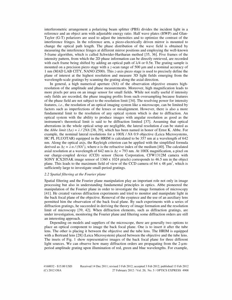
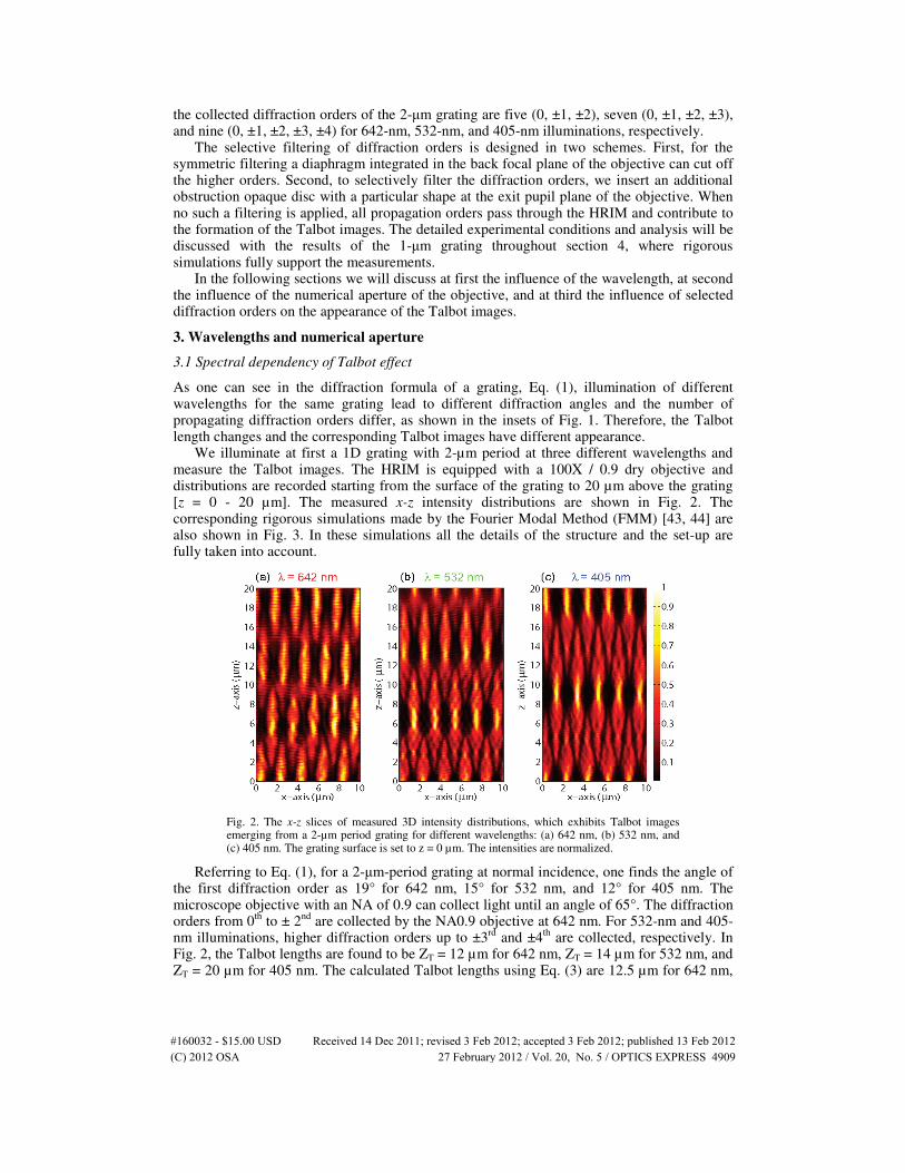
We illuminate at first a 1D grating with 2-µm period at three different wavelengths and measure the Talbot images. The HRIM is equipped with a 100X / 0.9 dry objective and distributions are recorded starting from the surface of the grating to 20 µm above the grating [z = 0 - 20 µm]. The measured x-z intensity distributions are shown in Fig. 2. The corresponding rigorous simulations made by the Fourier Modal Method (FMM) [43, 44] are also shown in Fig. 3. In these simulations all the details of the structure and the set-up are fully taken into account.

Fig. 2. The x-z slices of measured 3D intensity distributions, which exhibits Talbot images emerging from a 2-µm period grating for different wavelengths: (a) 642 nm, (b) 532 nm, and (c) 405 nm. The grating surface is set to z = 0 µm. The intensities are normalized.

Referring to Eq. (1), for a 2-µm-period grating at normal incidence, one finds the angle of the first diffraction order as 19° for 642 nm, 15° for 532 nm, and 12° for 405 nm. The microscope objective with an NA of 0.9 can collect light until an angle of 65°. The diffraction orders from 0

th to ± 2

nd are collected by the NA0.9 objective at 642 nm. For 532-nm and 405-

nm illuminations, higher diffraction orders up to ±3rd

and ±4th

are collected, respectively. In Fig. 2, the Talbot lengths are found to be ZT = 12 µm for 642 nm, ZT = 14 µm for 532 nm, and ZT = 20 µm for 405 nm. The calculated Talbot lengths using Eq. (3) are 12.5 µm for 642 nm,


15 µm for 532 nm, and 19.8 µm for 405 nm. The measured values show excellent agreement with the analytical solution.

One observes self-images at ZT and shifted self-images at half of the Talbot length (ZT/2) as could be expected [7, 8]. The visibility of the smaller fractions and sub-Talbot images differs because the number of collected diffraction orders and the intensity of each diffraction order vary for different wavelengths.

x−axis ( µm)

z−

ax

is (

µm

)

0 2 4 6 8 100

2

4

6

8

10

12

14

16

18

20

λ = 642 nm

x−axis ( µm)

z−

ax

is (

µm

)

0 2 4 6 8 100

2

4

6

8

10

12

14

16

18

20

λ = 532 nm λ = 405 nm

x−axis ( µm)

z−

ax

is (

µm

)

0 2 4 6 8 100

2

4

6

8

10

12

14

16

18

20

0.1

0.2

0.3

0.4

0.5

0.6

0.7

0.8

0.9

1

(a) (b) (c)

Fig. 3. The x-z slices of simulated 3D intensity distributions for a 2-µm period grating at different wavelengths (corresponding to Fig. 2): (a) 642 nm, (b) 532 nm, and (c) 405 nm. The intensities are normalized and the grating surface is at z = 0 µm.

3.2 Refractive index dependency of Talbot effect

The wavelength of light in an optically dense medium λmedium becomes shorter and is inversely proportional to the refractive index of the medium n:

.medium

n

λλ = (4)

Therefore, when the grating is immersed in a medium, the diffraction angle will be smaller compared to that in air. For instance, Eq. (1) leads to a diffraction angle of the first diffraction order of 12° for Λ = 2 µm, λ = 642 nm and n = 1.5. This eventually leads to analogous consequences as seen for the spectral dependency, which is discussed above in section 3.1.

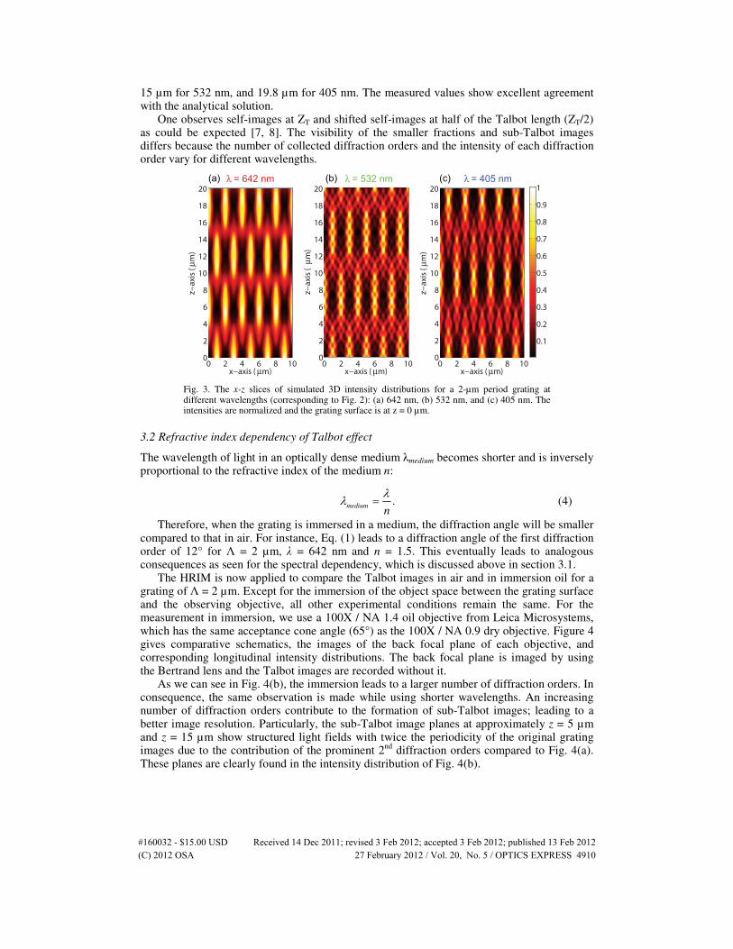
The HRIM is now applied to compare the Talbot images in air and in immersion oil for a grating of Λ = 2 µm. Except for the immersion of the object space between the grating surface and the observing objective, all other experimental conditions remain the same. For the measurement in immersion, we use a 100X / NA 1.4 oil objective from Leica Microsystems, which has the same acceptance cone angle (65°) as the 100X / NA 0.9 dry objective. Figure 4 gives comparative schematics, the images of the back focal plane of each objective, and corresponding longitudinal intensity distributions. The back focal plane is imaged by using the Bertrand lens and the Talbot images are recorded without it.

As we can see in Fig. 4(b), the immersion leads to a larger number of diffraction orders. In consequence, the same observation is made while using shorter wavelengths. An increasing number of diffraction orders contribute to the formation of sub-Talbot images; leading to a better image resolution. Particularly, the sub-Talbot image planes at approximately z = 5 µm and z = 15 µm show structured light fields with twice the periodicity of the original grating images due to the contribution of the prominent 2

nd diffraction orders compared to Fig. 4(a).

These planes are clearly found in the intensity distribution of Fig. 4(b).


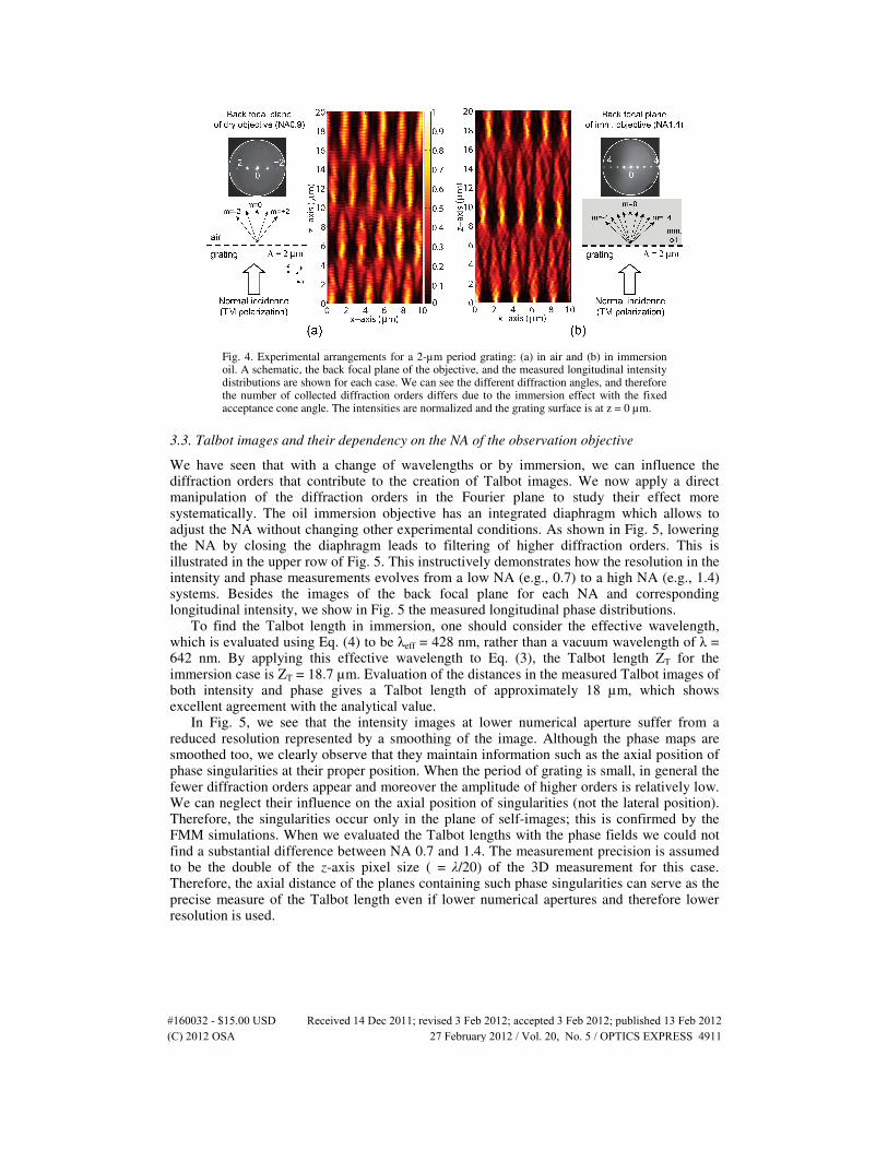
Fig. 4. Experimental arrangements for a 2-µm period grating: (a) in air and (b) in immersion oil. A schematic, the back focal plane of the objective, and the measured longitudinal intensity distributions are shown for each case. We can see the different diffraction angles, and therefore the number of collected diffraction orders differs due to the immersion effect with the fixed acceptance cone angle. The intensities are normalized and the grating surface is at z = 0 µm.

3.3. Talbot images and their dependency on the NA of the observation objective

We have seen that with a change of wavelengths or by immersion, we can influence the diffraction orders that contribute to the creation of Talbot images. We now apply a direct manipulation of the diffraction orders in the Fourier plane to study their effect more systematically. The oil immersion objective has an integrated diaphragm which allows to adjust the NA without changing other experimental conditions. As shown in Fig. 5, lowering the NA by closing the diaphragm leads to filtering of higher diffraction orders. This is illustrated in the upper row of Fig. 5. This instructively demonstrates how the resolution in the intensity and phase measurements evolves from a low NA (e.g., 0.7) to a high NA (e.g., 1.4) systems. Besides the images of the back focal plane for each NA and corresponding longitudinal intensity, we show in Fig. 5 the measured longitudinal phase distributions.

To find the Talbot length in immersion, one should consider the effective wavelength, which is evaluated using Eq. (4) to be λeff = 428 nm, rather than a vacuum wavelength of λ = 642 nm. By applying this effective wavelength to Eq. (3), the Talbot length ZT for the immersion case is ZT = 18.7 µm. Evaluation of the distances in the measured Talbot images of both intensity and phase gives a Talbot length of approximately 18 µm, which shows excellent agreement with the analytical value.

In Fig. 5, we see that the intensity images at lower numerical aperture suffer from a reduced resolution represented by a smoothing of the image. Although the phase maps are smoothed too, we clearly observe that they maintain information such as the axial position of phase singularities at their proper position. When the period of grating is small, in general the fewer diffraction orders appear and moreover the amplitude of higher orders is relatively low. We can neglect their influence on the axial position of singularities (not the lateral position). Therefore, the singularities occur only in the plane of self-images; this is confirmed by the FMM simulations. When we evaluated the Talbot lengths with the phase fields we could not find a substantial difference between NA 0.7 and 1.4. The measurement precision is assumed to be the double of the z-axis pixel size ( = λ/20) of the 3D measurement for this case. Therefore, the axial distance of the planes containing such phase singularities can serve as the precise measure of the Talbot length even if lower numerical apertures and therefore lower resolution is used.


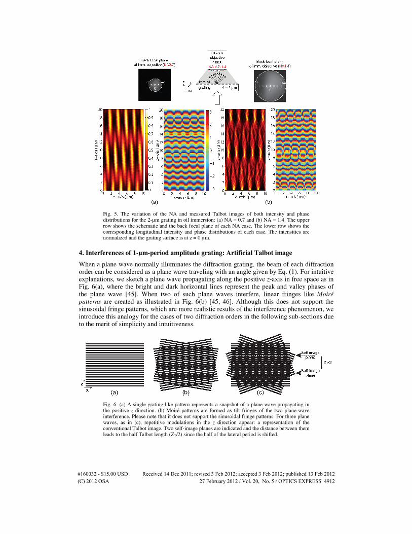
Fig. 5. The variation of the NA and measured Talbot images of both intensity and phase distributions for the 2-µm grating in oil immersion: (a) NA = 0.7 and (b) NA = 1.4. The upper row shows the schematic and the back focal plane of each NA case. The lower row shows the corresponding longitudinal intensity and phase distributions of each case. The intensities are normalized and the grating surface is at z = 0 µm.

4. Interferences of 1-µm-period amplitude grating: Artificial Talbot image

When a plane wave normally illuminates the diffraction grating, the beam of each diffraction order can be considered as a plane wave traveling with an angle given by Eq. (1). For intuitive explanations, we sketch a plane wave propagating along the positive z-axis in free space as in Fig. 6(a), where the bright and dark horizontal lines represent the peak and valley phases of the plane wave [45]. When two of such plane waves interfere, linear fringes like Moiré patterns are created as illustrated in Fig. 6(b) [45, 46]. Although this does not support the sinusoidal fringe patterns, which are more realistic results of the interference phenomenon, we introduce this analogy for the cases of two diffraction orders in the following sub-sections due to the merit of simplicity and intuitiveness.

Fig. 6. (a) A single grating-like pattern represents a snapshot of a plane wave propagating in the positive z direction. (b) Moiré patterns are formed as tilt fringes of the two plane-wave interference. Please note that it does not support the sinusoidal fringe patterns. For three plane waves, as in (c), repetitive modulations in the z direction appear: a representation of the conventional Talbot image. Two self-image planes are indicated and the distance between them leads to the half Talbot length (ZT/2) since the half of the lateral period is shifted.


In the case of Fig. 6(b), lateral periodic patterns can be observed in every plane perpendicular to the axial direction (z-axis) as the bright and dark fringes repeat along the lateral direction (x-axis). Consequently, no axial periodicity appears. Please note that in the bright fringe the overlap of the wavefront lines does not mean an actual fringe. This implies that two waves meet in-phase and the result is a bright stripe compared to the dark stripe in the out-of-phase situation. Thus, Fig. 6(b) does not represent a conventional Talbot image, which repeatedly appears at regular distances along the axial direction. To produce intensity modulation along the axial direction in such linear fringes, another plane wave is necessary. In such a three-plane-wave interference, periodic patterns along the z-axis are produced, as shown in Fig. 6(c). A minimum of three diffraction orders (plane waves) is therefore required to form a conventional Talbot image [27]. Our setup allows us to experimentally prove such behaviors because we can selectively block or manipulate diffraction orders in the back focal plane and verify their contribution to the Talbot images.

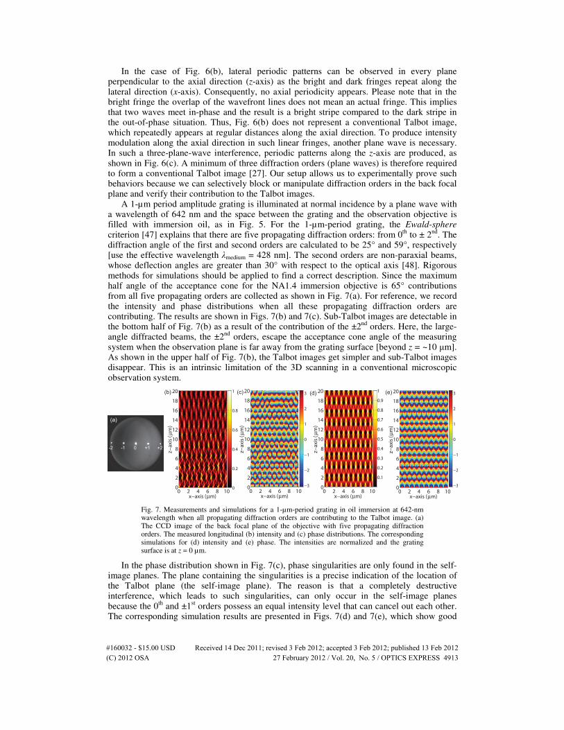
A 1-µm period amplitude grating is illuminated at normal incidence by a plane wave with a wavelength of 642 nm and the space between the grating and the observation objective is filled with immersion oil, as in Fig. 5. For the 1-µm-period grating, the Ewald-sphere criterion [47] explains that there are five propagating diffraction orders: from 0

th to ± 2

nd. The

diffraction angle of the first and second orders are calculated to be 25° and 59°, respectively [use the effective wavelength λmedium = 428 nm]. The second orders are non-paraxial beams, whose deflection angles are greater than 30° with respect to the optical axis [48]. Rigorous methods for simulations should be applied to find a correct description. Since the maximum half angle of the acceptance cone for the NA1.4 immersion objective is 65° contributions from all five propagating orders are collected as shown in Fig. 7(a). For reference, we record the intensity and phase distributions when all these propagating diffraction orders are contributing. The results are shown in Figs. 7(b) and 7(c). Sub-Talbot images are detectable in the bottom half of Fig. 7(b) as a result of the contribution of the ±2

nd orders. Here, the large-

angle diffracted beams, the ±2nd

orders, escape the acceptance cone angle of the measuring system when the observation plane is far away from the grating surface [beyond z = ~10 µm]. As shown in the upper half of Fig. 7(b), the Talbot images get simpler and sub-Talbot images disappear. This is an intrinsic limitation of the 3D scanning in a conventional microscopic observation system.

x−axis (µm)

z−

ax

is (

µm

)

0 2 4 6 8 100

2

4

6

8

10

12

14

16

18

20

0

0.2

0.4

0.6

0.8

1

x−axis (µm)

z−

ax

is (

µm

)

0 2 4 6 8 100

2

4

6

8

10

12

14

16

18

20

−3

−2

−1

0

1

2

3

−3

−2

−1

0

1

2

3(b) (c)

x−axis (µm)

z−

ax

is (

µm

)

0 2 4 6 8 100

2

4

6

8

10

12

14

16

18

20

x−axis (µm)

z−

ax

is (

µm

)

0 2 4 6 8 100

2

4

6

8

10

12

14

16

18

20(d) (e)

0-2 -1 +1 +2

(a)

0.1

0.2

0.3

0.4

0.5

0.6

0.7

0.8

0.9

1

Fig. 7. Measurements and simulations for a 1-µm-period grating in oil immersion at 642-nm wavelength when all propagating diffraction orders are contributing to the Talbot image. (a) The CCD image of the back focal plane of the objective with five propagating diffraction orders. The measured longitudinal (b) intensity and (c) phase distributions. The corresponding simulations for (d) intensity and (e) phase. The intensities are normalized and the grating surface is at z = 0 µm.

In the phase distribution shown in Fig. 7(c), phase singularities are only found in the self-image planes. The plane containing the singularities is a precise indication of the location of the Talbot plane (the self-image plane). The reason is that a completely destructive interference, which leads to such singularities, can only occur in the self-image planes because the 0

th and ±1

st orders possess an equal intensity level that can cancel out each other.

The corresponding simulation results are presented in Figs. 7(d) and 7(e), which show good


agreement for both intensity and phase distributions compared to Figs. 7(b) and 7(c). A phase wrapping along the longitudinal direction occurs intrinsically due to the modulation of the optical path length (OPL) in the interferometry during the z-axis scanning. This is an effect caused by the immersion scheme: while scanning the sample along the z-axis, the distance between the sample and the objective is changed that leads to a variation of the effective optical path length of the reference arm, which can be written as

( ) ,oil air

OPL n n l∆ = − ⋅ (5)

where l is the scanning distance and n is the refractive index of indicated material, oil or air. The period of such a phase wrapping is therefore inversely proportional to the refractive index difference of the immersion media and air [= noil – nair]. The measured wrapped images show a periodicity which is approximately 2 times larger than the operation wavelength for the oil immersion case (noil = 1.5). This has to be considered for the numerical simulation of the phase distributions and the results show excellent agreement with the measured phase maps.

Different filtering situations will be simulated in the following sub-sections. For easier interpretations, we always monitor the contributing diffraction orders to the artificial Talbot images for each experimental arrangement. Please note that the images presented in the following sections are not real Talbot images from the grating; the beams of each diffraction order are artificially manipulated and the results are the interference between selected diffraction orders. In order to individually block diffraction orders, we insert opaque screens of different shapes in the exit pupil of the objective. The higher diffraction orders can also be symmetrically filtered out by the objective diaphragm in the back focal plane.

4.1 A single diffraction order: The 0th

order

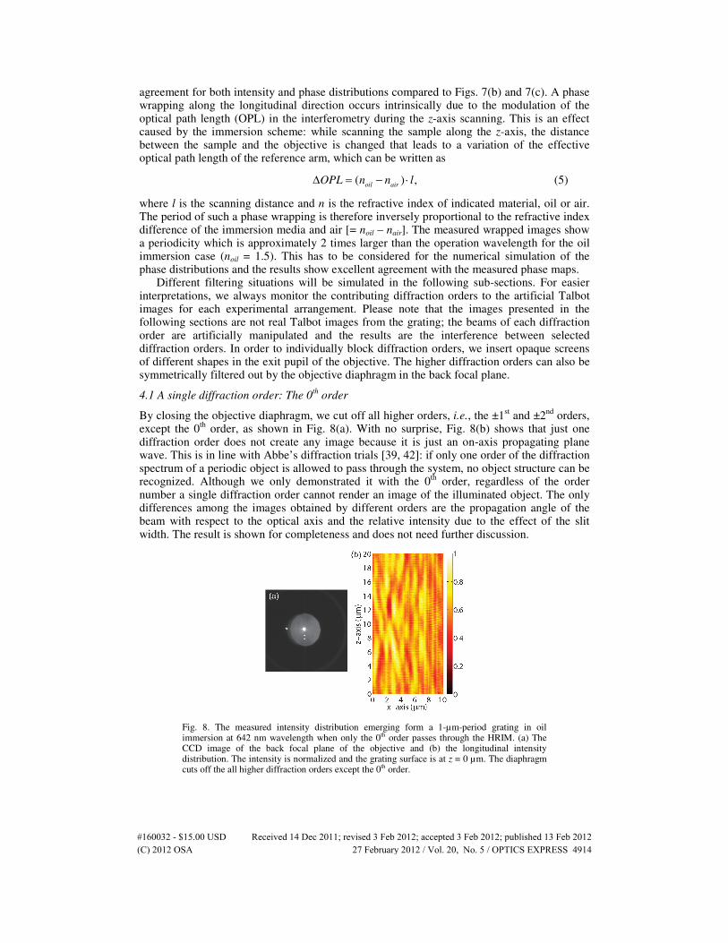
By closing the objective diaphragm, we cut off all higher orders, i.e., the ±1st and ±2

nd orders,

except the 0th

order, as shown in Fig. 8(a). With no surprise, Fig. 8(b) shows that just one diffraction order does not create any image because it is just an on-axis propagating plane wave. This is in line with Abbe’s diffraction trials [39, 42]: if only one order of the diffraction spectrum of a periodic object is allowed to pass through the system, no object structure can be recognized. Although we only demonstrated it with the 0

th order, regardless of the order

number a single diffraction order cannot render an image of the illuminated object. The only differences among the images obtained by different orders are the propagation angle of the beam with respect to the optical axis and the relative intensity due to the effect of the slit width. The result is shown for completeness and does not need further discussion.

Fig. 8. The measured intensity distribution emerging form a 1-µm-period grating in oil immersion at 642 nm wavelength when only the 0th order passes through the HRIM. (a) The CCD image of the back focal plane of the objective and (b) the longitudinal intensity distribution. The intensity is normalized and the grating surface is at z = 0 µm. The diaphragm cuts off the all higher diffraction orders except the 0th order.


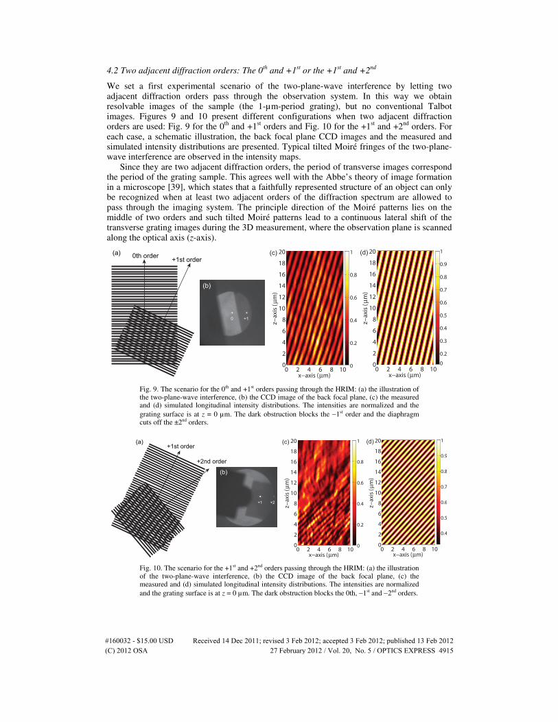
4.2 Two adjacent diffraction orders: The 0th

and +1st or the +1

st and +2

nd

We set a first experimental scenario of the two-plane-wave interference by letting two adjacent diffraction orders pass through the observation system. In this way we obtain resolvable images of the sample (the 1-µm-period grating), but no conventional Talbot images. Figures 9 and 10 present different configurations when two adjacent diffraction orders are used: Fig. 9 for the 0

th and +1

st orders and Fig. 10 for the +1

st and +2

nd orders. For

each case, a schematic illustration, the back focal plane CCD images and the measured and simulated intensity distributions are presented. Typical tilted Moiré fringes of the two-plane-wave interference are observed in the intensity maps.

Since they are two adjacent diffraction orders, the period of transverse images correspond the period of the grating sample. This agrees well with the Abbe’s theory of image formation in a microscope [39], which states that a faithfully represented structure of an object can only be recognized when at least two adjacent orders of the diffraction spectrum are allowed to pass through the imaging system. The principle direction of the Moiré patterns lies on the middle of two orders and such tilted Moiré patterns lead to a continuous lateral shift of the transverse grating images during the 3D measurement, where the observation plane is scanned along the optical axis (z-axis).

x−axis (µm)

z−

ax

is (

µm

)

0 2 4 6 8 100

2

4

6

8

10

12

14

16

18

20

0

0.2

0.4

0.6

0.8

1

0.2

0.3

0.4

0.5

0.6

0.7

0.8

0.9

1

0

0 +1

(b)

(c)(a) 0th order+1st order

x−axis (µm)

z−

ax

is (

µm

)

0 2 4 6 8 100

2

4

6

8

10

12

14

16

18

20(d)

Fig. 9. The scenario for the 0th and +1st orders passing through the HRIM: (a) the illustration of the two-plane-wave interference, (b) the CCD image of the back focal plane, (c) the measured and (d) simulated longitudinal intensity distributions. The intensities are normalized and the

grating surface is at z = 0 µm. The dark obstruction blocks the −1st order and the diaphragm cuts off the ±2nd orders.

+1 +2

x−axis (µm)

z−

ax

is (

µm

)

0 2 4 6 8 100

2

4

6

8

10

12

14

16

18

20

0

0.2

0.4

0.6

0.8

1

(b)

(c)(a)

x−axis (µm)

z−

ax

is (

µm

)

0 2 4 6 8 100

2

4

6

8

10

12

14

16

18

20(d)

+2nd order

+1st order

0.4

0.5

0.6

0.7

0.8

0.9

1

Fig. 10. The scenario for the +1st and +2nd orders passing through the HRIM: (a) the illustration of the two-plane-wave interference, (b) the CCD image of the back focal plane, (c) the measured and (d) simulated longitudinal intensity distributions. The intensities are normalized

and the grating surface is at z = 0 µm. The dark obstruction blocks the 0th, −1st and −2nd orders.


When the observation plane is moved far away from the grating surface, higher diffraction orders, which have large diffraction angle with respect to the optical axis, escape the cone of the acceptance angle of the objective given by the NA. Consequently, the diffracted beam with a larger angle, i.e., the +2

nd order, escapes the acceptance cone angle of the measuring

system after z = ~10 µm. In general, this causes smoothening of the Talbot images and the suppression of the sub-Talbot images. In the discussion we concentrate on feature appearing within the region close to the grating, where such higher orders contribute to the formation of the Talbot images. This effect is visible in the upper half of Fig. 10(b), where no interference fringes occur, compared to Fig. 10(c). Except this, the, measurement is in good agreement with rigorous simulation result.

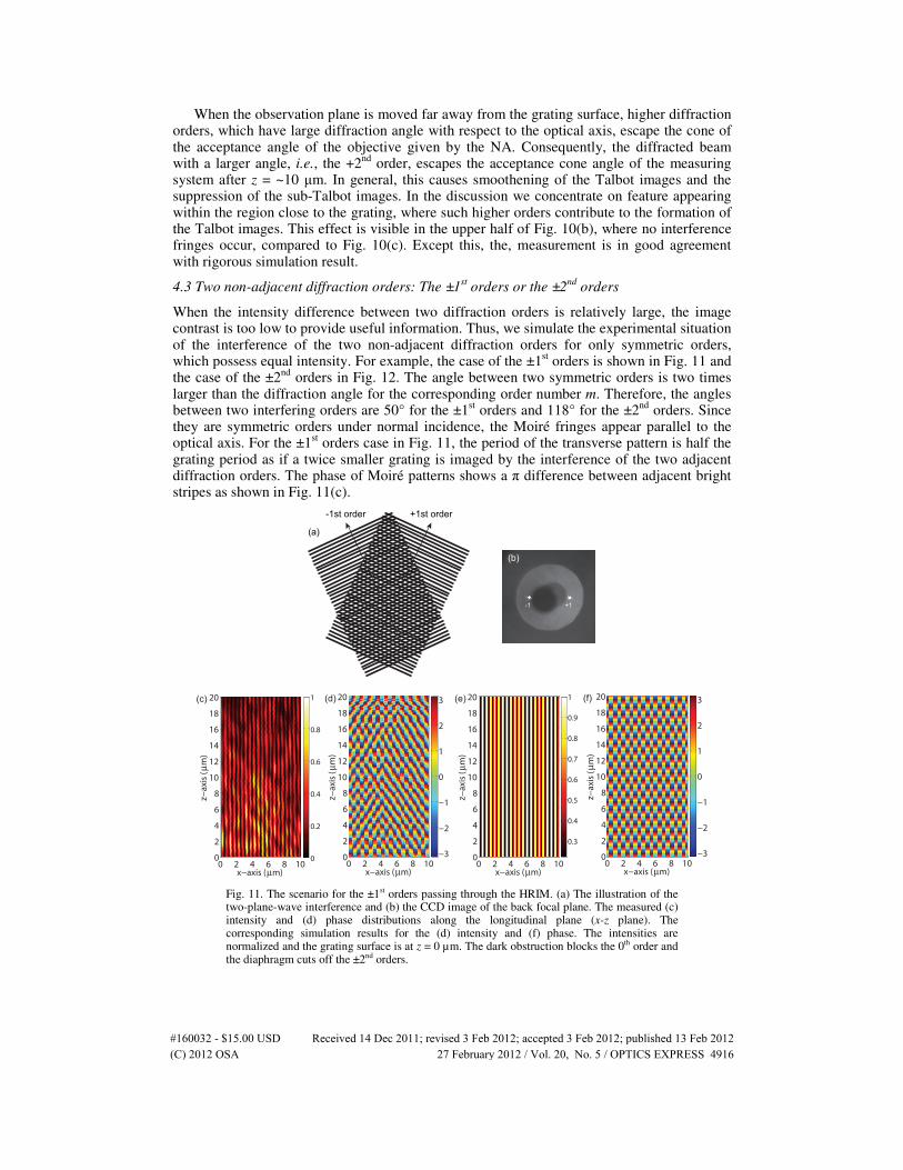
4.3 Two non-adjacent diffraction orders: The ±1st orders or the ±2

nd orders

When the intensity difference between two diffraction orders is relatively large, the image contrast is too low to provide useful information. Thus, we simulate the experimental situation of the interference of the two non-adjacent diffraction orders for only symmetric orders, which possess equal intensity. For example, the case of the ±1

st orders is shown in Fig. 11 and

the case of the ±2nd

orders in Fig. 12. The angle between two symmetric orders is two times larger than the diffraction angle for the corresponding order number m. Therefore, the angles between two interfering orders are 50° for the ±1

st orders and 118° for the ±2

nd orders. Since

they are symmetric orders under normal incidence, the Moiré fringes appear parallel to the optical axis. For the ±1

st orders case in Fig. 11, the period of the transverse pattern is half the

grating period as if a twice smaller grating is imaged by the interference of the two adjacent diffraction orders. The phase of Moiré patterns shows a π difference between adjacent bright stripes as shown in Fig. 11(c).

-1 +1

(b)

(a)

+1st order-1st order

x−axis (µm)

z−

ax

is (

µm

)

0 2 4 6 8 100

2

4

6

8

10

12

14

16

18

20

0

0.2

0.4

0.6

0.8

1

0.3

0.4

0.5

0.6

0.7

0.8

0.9

1(c)

x−axis (µm)

z−

ax

is (

µm

)

0 2 4 6 8 100

2

4

6

8

10

12

14

16

18

20(d)

−3

−2

−1

0

1

2

3

x−axis (µm)

z−

ax

is (

µm

)

0 2 4 6 8 100

2

4

6

8

10

12

14

16

18

20(e)

x−axis (µm)

z−

ax

is (

µm

)

0 2 4 6 8 100

2

4

6

8

10

12

14

16

18

20(f)

−3

−2

−1

0

1

2

3

Fig. 11. The scenario for the ±1st orders passing through the HRIM. (a) The illustration of the two-plane-wave interference and (b) the CCD image of the back focal plane. The measured (c) intensity and (d) phase distributions along the longitudinal plane (x-z plane). The corresponding simulation results for the (d) intensity and (f) phase. The intensities are normalized and the grating surface is at z = 0 µm. The dark obstruction blocks the 0th order and the diaphragm cuts off the ±2nd orders.


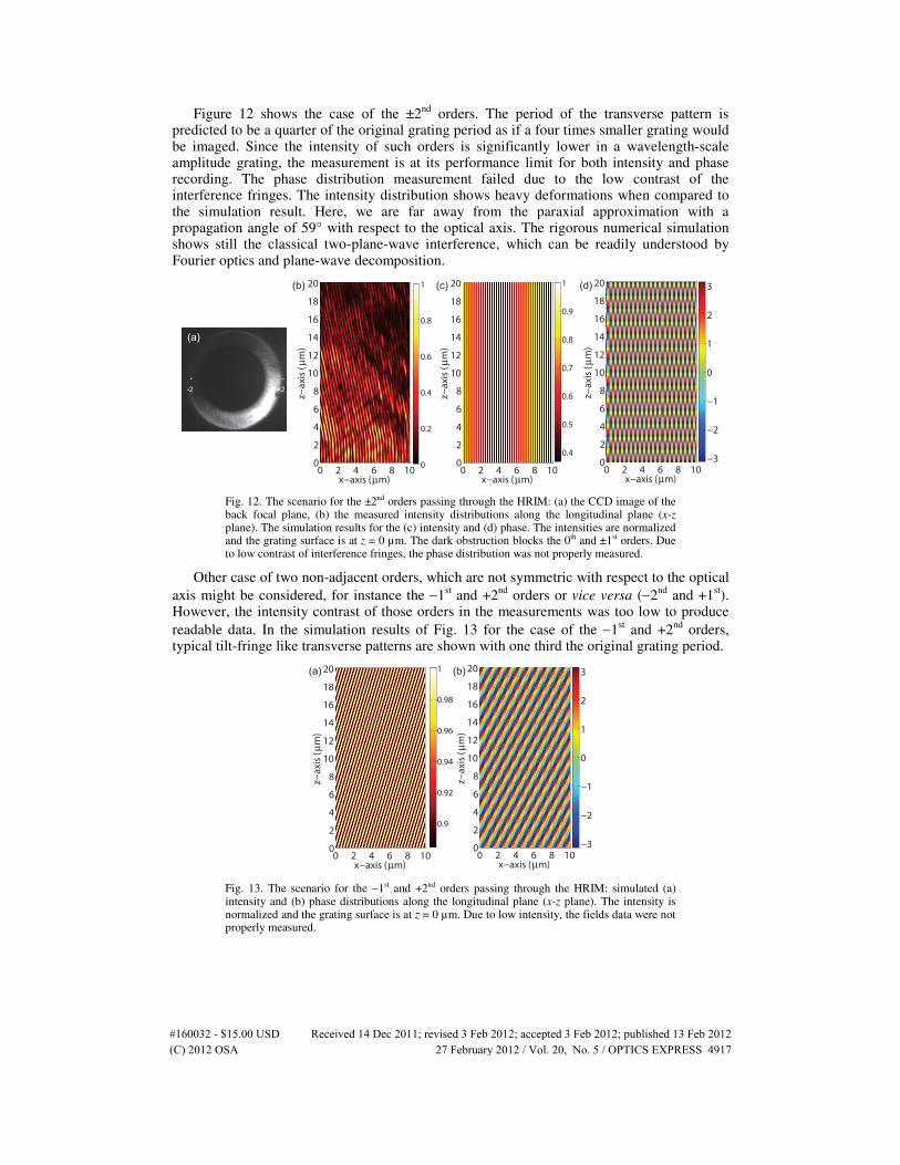
Figure 12 shows the case of the ±2nd

orders. The period of the transverse pattern is predicted to be a quarter of the original grating period as if a four times smaller grating would be imaged. Since the intensity of such orders is significantly lower in a wavelength-scale amplitude grating, the measurement is at its performance limit for both intensity and phase recording. The phase distribution measurement failed due to the low contrast of the interference fringes. The intensity distribution shows heavy deformations when compared to the simulation result. Here, we are far away from the paraxial approximation with a propagation angle of 59° with respect to the optical axis. The rigorous numerical simulation shows still the classical two-plane-wave interference, which can be readily understood by Fourier optics and plane-wave decomposition.

x−axis (µm)

z−

ax

is (

µm

)

0 2 4 6 8 100

2

4

6

8

10

12

14

16

18

20

x−axis (µm)

z−

ax

is (

µm

)

0 2 4 6 8 100

2

4

6

8

10

12

14

16

18

20(c)

x−axis (µm)

z−

ax

is (

µm

)

0 2 4 6 8 100

2

4

6

8

10

12

14

16

18

20(d)

−3

−2

−1

0

1

2

3

0

0.2

0.4

0.6

0.8

1

0.4

0.5

0.6

0.7

0.8

0.9

1

-2 +2

(a)

(b)

Fig. 12. The scenario for the ±2nd orders passing through the HRIM: (a) the CCD image of the back focal plane, (b) the measured intensity distributions along the longitudinal plane (x-z plane). The simulation results for the (c) intensity and (d) phase. The intensities are normalized and the grating surface is at z = 0 µm. The dark obstruction blocks the 0th and ±1st orders. Due to low contrast of interference fringes, the phase distribution was not properly measured.

Other case of two non-adjacent orders, which are not symmetric with respect to the optical

axis might be considered, for instance the −1st and +2

nd orders or vice versa (−2

nd and +1

st).

However, the intensity contrast of those orders in the measurements was too low to produce

readable data. In the simulation results of Fig. 13 for the case of the −1st and +2

nd orders,

typical tilt-fringe like transverse patterns are shown with one third the original grating period.

x−axis (µm)

z−

ax

is (

µm

)

0 2 4 6 8 100

2

4

6

8

10

12

14

16

18

20(a)

x−axis (µm)

z−

ax

is (

µm

)

0 2 4 6 8 100

2

4

6

8

10

12

14

16

18

20(b)

−3

−2

−1

0

1

2

3

0.9

0.92

0.94

0.96

0.98

1

Fig. 13. The scenario for the −1st and +2nd orders passing through the HRIM: simulated (a) intensity and (b) phase distributions along the longitudinal plane (x-z plane). The intensity is normalized and the grating surface is at z = 0 µm. Due to low intensity, the fields data were not properly measured.


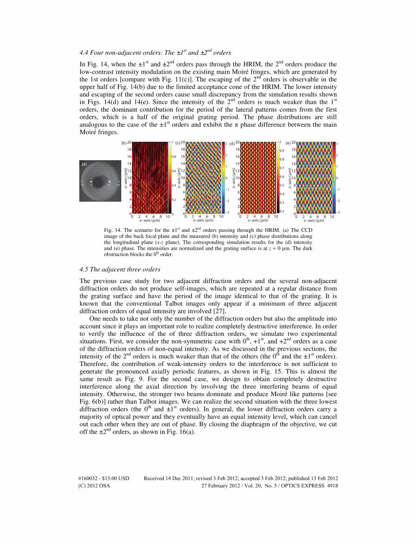
4.4 Four non-adjacent orders: The ±1st and ±2

nd orders

In Fig. 14, when the ±1st and ±2

nd orders pass through the HRIM, the 2

nd orders produce the

low-contrast intensity modulation on the existing main Moiré fringes, which are generated by the 1st orders [compare with Fig. 11(c)]. The escaping of the 2

nd orders is observable in the

upper half of Fig. 14(b) due to the limited acceptance cone of the HRIM. The lower intensity and escaping of the second orders cause small discrepancy from the simulation results shown in Figs. 14(d) and 14(e). Since the intensity of the 2

nd orders is much weaker than the 1

st

orders, the dominant contribution for the period of the lateral patterns comes from the first orders, which is a half of the original grating period. The phase distributions are still analogous to the case of the ±1

st orders and exhibit the π phase difference between the main

Moiré fringes.

-1 +1

(a)

-2 +2

x−axis (µm)

z−

ax

is (

µm

)

0 2 4 6 8 100

2

4

6

8

10

12

14

16

18

20

0

0.2

0.4

0.6

0.8

1

x−axis (µm)

z−

ax

is (

µm

)

0 2 4 6 8 100

2

4

6

8

10

12

14

16

18

20

−3

−2

−1

0

1

2

3

−3

−2

−1

0

1

2

3(b) (c)

x−axis (µm)

z−

ax

is (

µm

)

0 2 4 6 8 100

2

4

6

8

10

12

14

16

18

20

x−axis (µm)

z−

ax

is (

µm

)

0 2 4 6 8 100

2

4

6

8

10

12

14

16

18

20(d) (e)

0.2

0.3

0.4

0.5

0.6

0.7

0.8

0.9

1

Fig. 14. The scenario for the ±1st and ±2nd orders passing through the HRIM. (a) The CCD image of the back focal plane and the measured (b) intensity and (c) phase distributions along the longitudinal plane (x-z plane). The corresponding simulation results for the (d) intensity and (e) phase. The intensities are normalized and the grating surface is at z = 0 µm. The dark obstruction blocks the 0th order.

4.5 The adjacent three orders

The previous case study for two adjacent diffraction orders and the several non-adjacent diffraction orders do not produce self-images, which are repeated at a regular distance from the grating surface and have the period of the image identical to that of the grating. It is known that the conventional Talbot images only appear if a minimum of three adjacent diffraction orders of equal intensity are involved [27].

One needs to take not only the number of the diffraction orders but also the amplitude into account since it plays an important role to realize completely destructive interference. In order to verify the influence of the of three diffraction orders, we simulate two experimental situations. First, we consider the non-symmetric case with 0

th, +1

st, and +2

nd orders as a case

of the diffraction orders of non-equal intensity. As we discussed in the previous sections, the intensity of the 2

nd orders is much weaker than that of the others (the 0

th and the ±1

st orders).

Therefore, the contribution of weak-intensity orders to the interference is not sufficient to generate the pronounced axially periodic features, as shown in Fig. 15. This is almost the same result as Fig. 9. For the second case, we design to obtain completely destructive interference along the axial direction by involving the three interfering beams of equal intensity. Otherwise, the stronger two beams dominate and produce Moiré like patterns [see Fig. 6(b)] rather than Talbot images. We can realize the second situation with the three lowest diffraction orders (the 0

th and ±1

st orders). In general, the lower diffraction orders carry a

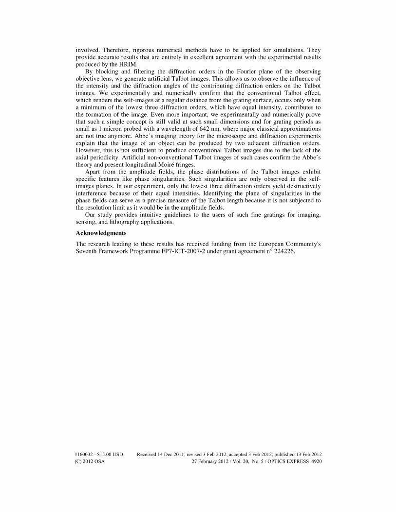
majority of optical power and they eventually have an equal intensity level, which can cancel out each other when they are out of phase. By closing the diaphragm of the objective, we cut off the ±2

nd orders, as shown in Fig. 16(a).


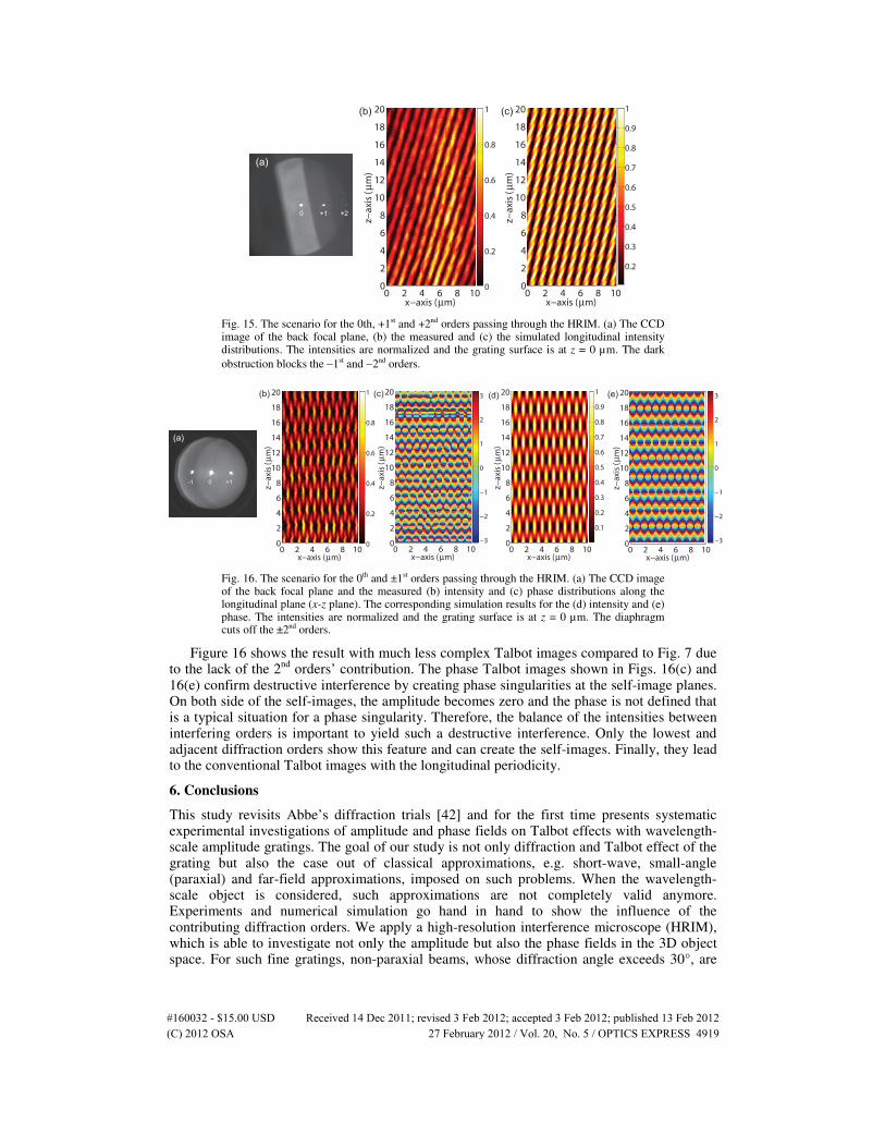
x−axis (µm)

z−

ax

is (

µm

)

0 2 4 6 8 100

2

4

6

8

10

12

14

16

18

20

x−axis (µm)

z−

ax

is (

µm

)

0 2 4 6 8 100

2

4

6

8

10

12

14

16

18

20(c)

0

0.2

0.4

0.6

0.8

1

0.2

0.3

0.4

0.5

0.6

0.7

0.8

0.9

1

0 +1

(a)

+2

(b)

Fig. 15. The scenario for the 0th, +1st and +2nd orders passing through the HRIM. (a) The CCD image of the back focal plane, (b) the measured and (c) the simulated longitudinal intensity distributions. The intensities are normalized and the grating surface is at z = 0 µm. The dark

obstruction blocks the −1st and −2nd orders.

x−axis (µm)

z−

ax

is (

µm

)

0 2 4 6 8 100

2

4

6

8

10

12

14

16

18

20

0

0.2

0.4

0.6

0.8

1

x−axis (µm)

z−

ax

is (

µm

)

0 2 4 6 8 100

2

4

6

8

10

12

14

16

18

20

−3

−2

−1

0

1

2

3

−3

−2

−1

0

1

2

3(b) (c)

0-1 +1

(a)

x−axis (µm)

z−

ax

is (

µm

)

0 2 4 6 8 100

2

4

6

8

10

12

14

16

18

20

x−axis (µm)

z−

ax

is (

µm

)

0 2 4 6 8 100

2

4

6

8

10

12

14

16

18

20(d) (e)

0.1

0.2

0.3

0.4

0.5

0.6

0.7

0.8

0.9

1

Fig. 16. The scenario for the 0th and ±1st orders passing through the HRIM. (a) The CCD image of the back focal plane and the measured (b) intensity and (c) phase distributions along the longitudinal plane (x-z plane). The corresponding simulation results for the (d) intensity and (e) phase. The intensities are normalized and the grating surface is at z = 0 µm. The diaphragm cuts off the ±2nd orders.

Figure 16 shows the result with much less complex Talbot images compared to Fig. 7 due to the lack of the 2

nd orders’ contribution. The phase Talbot images shown in Figs. 16(c) and

16(e) confirm destructive interference by creating phase singularities at the self-image planes. On both side of the self-images, the amplitude becomes zero and the phase is not defined that is a typical situation for a phase singularity. Therefore, the balance of the intensities between interfering orders is important to yield such a destructive interference. Only the lowest and adjacent diffraction orders show this feature and can create the self-images. Finally, they lead to the conventional Talbot images with the longitudinal periodicity.

6. Conclusions

This study revisits Abbe’s diffraction trials [42] and for the first time presents systematic experimental investigations of amplitude and phase fields on Talbot effects with wavelength-scale amplitude gratings. The goal of our study is not only diffraction and Talbot effect of the grating but also the case out of classical approximations, e.g. short-wave, small-angle (paraxial) and far-field approximations, imposed on such problems. When the wavelength-scale object is considered, such approximations are not completely valid anymore. Experiments and numerical simulation go hand in hand to show the influence of the contributing diffraction orders. We apply a high-resolution interference microscope (HRIM), which is able to investigate not only the amplitude but also the phase fields in the 3D object space. For such fine gratings, non-paraxial beams, whose diffraction angle exceeds 30°, are


involved. Therefore, rigorous numerical methods have to be applied for simulations. They provide accurate results that are entirely in excellent agreement with the experimental results produced by the HRIM.

By blocking and filtering the diffraction orders in the Fourier plane of the observing objective lens, we generate artificial Talbot images. This allows us to observe the influence of the intensity and the diffraction angles of the contributing diffraction orders on the Talbot images. We experimentally and numerically confirm that the conventional Talbot effect, which renders the self-images at a regular distance from the grating surface, occurs only when a minimum of the lowest three diffraction orders, which have equal intensity, contributes to the formation of the image. Even more important, we experimentally and numerically prove that such a simple concept is still valid at such small dimensions and for grating periods as small as 1 micron probed with a wavelength of 642 nm, where major classical approximations are not true anymore. Abbe’s imaging theory for the microscope and diffraction experiments explain that the image of an object can be produced by two adjacent diffraction orders. However, this is not sufficient to produce conventional Talbot images due to the lack of the axial periodicity. Artificial non-conventional Talbot images of such cases confirm the Abbe’s theory and present longitudinal Moiré fringes.

Apart from the amplitude fields, the phase distributions of the Talbot images exhibit specific features like phase singularities. Such singularities are only observed in the self-images planes. In our experiment, only the lowest three diffraction orders yield destructively interference because of their equal intensities. Identifying the plane of singularities in the phase fields can serve as a precise measure of the Talbot length because it is not subjected to the resolution limit as it would be in the amplitude fields.

Our study provides intuitive guidelines to the users of such fine gratings for imaging, sensing, and lithography applications.

Acknowledgments

The research leading to these results has received funding from the European Community's Seventh Framework Programme FP7-ICT-2007-2 under grant agreement n° 224226.


Documents

Talbot images of wavelength-scale amplitude gratings images of... · Talbot images of wavelength-scale amplitude gratings ... L. M. Sanchez-Brea, and J. Vargas, ... (Roberts & Company,