1  

Tail risk in hedge funds: A unique view from portfolio holdings

Vikas Agarwal, Stefan Ruenzi, and Florian Weigert

This Version: March 5, 2016

Abstract

We develop a new systematic tail risk measure for equity-oriented hedge funds to examine the impact of tail risk on fund performance and to identify the sources of tail risk. We find that tail risk affects the cross-sectional variation in fund returns, and investments in both, tail-sensitive stocks as well as options, drive tail risk. Moreover, leverage and exposure to funding liquidity shocks are important determinants of tail risk. We find evidence of some funds being able to time tail risk exposure prior to the recent financial crisis.

Keywords: Hedge Funds, Tail Risk, Portfolio Holdings, Funding Liquidity Risk JEL Classification Numbers: G11, G23

                                                             Vikas Agarwal is from Georgia State University, J. Mack Robinson College of Business, 35 Broad Street, Suite 1234, Atlanta GA 30303, USA. Email: vagarwal@gsu.edu.Tel: +1-404-413-7326. Fax: +1-404-413-7312. Vikas Agarwal is also a Research Fellow at the Centre for Financial Research (CFR), University of Cologne. Stefan Ruenzi is from the University of Mannheim, L9, 1-2, 68161 Mannheim, Germany. Email: ruenzi@bwl.uni-mannheim.de. Tel: +49-621-181-1646. Florian Weigert is from the University of St. Gallen, Swiss Institute of Banking and Finance, Rosenbergstrasse 52, 9000 St. Gallen, Switzerland. Email: florian.weigert@unisg.ch. Tel: +41-71-224-7014. We thank George Aragon, Turan Bali, Martin Brown, Stephen Brown, John Cochrane, Yong Chen, Andre Güttler, Olga Kolokolova, Jens Jackwerth, Juha Joenväärä, Petri Jylha, Marie Lambert, Tao Li, Bing Liang, Gunter Löffler, Scott Murray, George Panayotov, Liang Peng, Lubomir Petrasek, Alberto Plazzi, Paul Söderlind, and Fabio Trojani for their helpful comments and constructive suggestions. We benefited from the comments received at presentations at the 6th Annual Conference on Hedge Funds in Paris, the 9th Imperial Conference on Advances in the Analysis of Hedge Fund Strategies, the Berlin Asset Management Conference 2015, the CFEA 2015 Conference, the Annual Meeting of the German Finance Association 2015, the FMA 2015 conference, the FMA Consortium on Activist Investors, Corporate Governance and Hedge Funds 2015, the Luxembourg Asset Management Summit 2015, the National Taiwan University, the Purdue University, the University of Mannheim, the University of St. Gallen, and the University of Ulm. We would also like to thank Kevin Mullally and Honglin Ren for excellent research assistance.

2  

Tail risk in hedge funds: A unique view from portfolio holdings

This Version: February 25, 2016

Abstract

We develop a new systematic tail risk measure for equity-oriented hedge funds to examine the impact of tail risk on fund performance and to identify the sources of tail risk. We find that tail risk affects the cross-sectional variation in fund returns, and investments in both, tail-sensitive stocks as well as options, drive tail risk. Moreover, leverage and exposure to funding liquidity shocks are important determinants of tail risk. We find evidence of some funds being able to time tail risk exposure prior to the recent financial crisis.

Keywords: Hedge Funds, Tail Risk, Portfolio Holdings, Funding Liquidity Risk JEL Classification Numbers: G11, G23

3  

Tail risk in hedge funds: A unique view from portfolio holdings

Hedge funds are often described as pursuing trading strategies that generate small positive

returns most of the time before incurring a substantial loss akin to “picking up pennies in front

of a steam roller” or “selling earthquake insurance” (Duarte, Longstaff, and Yu, 2007; Stulz,

2007). Hedge funds are therefore likely to be exposed to substantial systematic tail risk, i.e.,

they can incur substantial losses in times of market downturns when investors’ marginal utility

is very high.1 However, there is limited research on whether hedge funds are exposed to tail

risk, and if so, how hedge funds’ investments and trading strategies contribute to tail risk and

how it affects hedge fund performance. Our paper fills this void in the literature by using

equity-oriented hedge fund return data as well as the mandatorily reported 13F quarterly equity

and option holdings of hedge fund firms to examine the sources and performance implications

of tail risk.2 In particular, we ask the following questions. First, does tail risk explain the cross-

sectional variation in equity-oriented hedge fund performance? Second, is tail risk related to

certain observable fund characteristics and funds’ exposure to funding liquidity shocks? Third,

does tail risk in hedge funds arise from their dynamic trading strategies and/or their investments

in stocks that are sensitive to equity market crashes? Finally, can hedge funds time tail risk by

altering their positions in equities and options before market crashes?

We address these questions by first deriving a non-parametric estimate for hedge funds’

systematic tail risk based on their reported returns. This tail risk measure is defined as the lower

tail dependence of hedge funds’ returns and the market return, scaled by the ratio of the absolute

value of their respective expected shortfalls (ES). The lower tail dependence is defined as the

conditional probability that an individual hedge fund has its worst individual return realizations

exactly at the same time when the equity market also has its worst return realizations in a given

                                                            1As an illustration, Figure A.1 plots monthly returns for the HFR Equal-Weighted Hedge Fund Strategy Index in the period from 1998 to 2012. The two worst return realizations occur in August 1998 and October 2008 which coincide with periods of severe equity market downturns (i.e., the Russian Financial Crisis in 1998 and the bankruptcy of Lehman Brothers in 2008, respectively). 2Institutional investors including hedge funds that exercise investment discretion over $100 million of assets in 13F securities are required to disclose their long positions in 13F securities (common stocks, convertible bonds, and options) on a quarterly basis. They are not required to report any short positions (see Griffin and Xu, 2009; Aragon and Martin, 2012; Agarwal, Fos, and Jiang, 2013; and Agarwal, Jiang, Yang, and Tang, 2013).

4  

time span. We show that this tail risk measure has significant predictive power for the cross-

section of equity-oriented hedge fund strategies.3 We find that the return spread between the

portfolios of hedge funds with the highest and the lowest past tail risk amounts to 4.68% per

annum after controlling for the risk factors in the widely used Fung and Hsieh (2004) 7-factor

model. These spreads are robust to controlling for other risks that have been shown to influence

hedge fund returns including correlation risk (Buraschi, Kosowski, and Trojani, 2014),

liquidity risk (Aragon, 2007; Sadka, 2010; Teo, 2011), macroeconomic uncertainty (Bali,

Brown, and Caglayan, 2014), volatility risk (Bondarenko, 2004; Agarwal, Bakshi, and Huij,

2009), and rare disaster concerns (Gao, Gao, and Song, 2014). In addition, results from

multivariate regressions confirm that tail risk predicts future fund returns even after controlling

for various fund characteristics such as fund size, age, standard deviation, delta, past yearly

excess return, management and incentive fees, minimum investment, lockup and restriction

period, and indicator variables for offshore domicile, leverage, high watermark, and hurdle

rate, as well as univariate risk measures such as skewness, kurtosis, value-at-risk (VaR), and

market beta. The predictability of future returns extends as far as six months into the future.

We conduct a number of robustness checks to show that these results are not sensitive

to several choices that we make in our empirical analysis. Our results are stable when we

change the estimation horizon of tail risk, compute tail risk using different cut-off values, use

VaR instead of ES in the computation of tail risk, change the weighting procedure in portfolio

sorts from equal-weighting to value-weighting, and account for delisting returns of funds that

leave the database. Our results also remain stable when we compute tail risk with daily instead

of monthly returns using data for a subsample of hedge funds that report daily data to

Bloomberg and only use returns reported after the listing date of a subsample of hedge funds

from the Lipper TASS database.

Next, we investigate the determinants of tail risk of hedge funds, i.e., why some funds

are more exposed to tail risk than others and which fund characteristics are associated with

high tail risk. We document several findings that are consistent with the earlier theoretical and

empirical literature on the relation between risk-taking behavior and contractual features of

                                                            3In principle, our investigation can be extended to non-equity hedge funds too, but we restrict ourselves to equity funds to link tail risk with the underlying holdings that are available only for equity positions.

5  

hedge funds. First, we find that the managerial incentives stemming from the incentive fee call

option are positively related to funds’ tail risk. This result is consistent with the risk-inducing

behavior associated with the call option feature of incentive fee contracts (Brown, Goetzmann,

and Park, 2001; Goetzmann, Ingersoll, and Ross, 2003; Hodder and Jackwerth, 2007). Second,

we observe that tail risk is negatively associated with past performance, i.e., worse performing

fund managers engage in greater risk-taking behavior. This finding is similar to the increase in

propensity to take risk following poor performance as documented in Aragon and Nanda

(2012). Finally, both the lockup period and leverage exhibit a significant positive relation with

tail risk. Since funds with longer lockup period are likely to invest in more illiquid securities

(Aragon, 2007), this finding suggests that funds that make such illiquid investments are more

likely to be exposed to higher tail risk. Levered funds may use derivatives and short selling

techniques to take state-contingent bets that can exacerbate tail risk in such funds.

We also use the bankruptcy of Lehman Brothers in September 2008 as a quasi-natural

experiment leading to an exogenous shock to the funding of hedge funds by prime brokers.

This allows us to examine a causal relation between funding liquidity risk and tail risk. We find

evidence of a greater increase in tail risk of funds that used Lehman Brothers as their prime

broker as compared to other funds, indicating that funding liquidity shocks can enhance tail

risk.

We next investigate different trading strategies that can induce tail risk in hedge funds

to shed light on the sources of tail risk. In particular, we consider (i) dynamic trading strategies

captured by exposures to a factor that mimics the return of short out-of-the-money put options

on the equity market of Agarwal and Naik (2004) as well as (ii) an investment strategy

involving long positions in high tail risk stocks and short positions in low tail risk stocks, i.e.,

exposure to an equity tail risk factor (Chabi-Yo, Ruenzi, and Weigert, 2015; Kelly and Jiang,

2014). To understand which of these strategies explain the tail risk of hedge funds, we first

regress individual hedge funds’ returns on the S&P 500 index put option factor as in Agarwal

and Naik (2004) and on the Chabi-Yo, Ruenzi, and Weigert (2015) equity tail risk factor. We

then analyze how the cross-sectional differences in hedge funds’ overall tail risk can be

explained by the funds’ exposures to these factors. We find that funds’ tail risk is negatively

related to the Agarwal and Naik (2004) out-of-the-money put option factor and positively

6  

related to the Chabi-Yo, Ruenzi, and Weigert (2015) equity tail risk factor. Ceteris paribus, a

one standard deviation decrease (increase) in the put option beta (equity tail risk beta) is

associated with an increase of overall tail risk by 0.26 (0.13). Given an average tail risk of

equity-related funds of 0.38, this translates into an increase of 68% and 34% in the tail risk for

a one standard deviation increase in the sensitivities to the put option factor and the equity tail

risk factor, respectively.

Motivated by the positive relation between hedge fund tail risk and return exposure to

the equity tail risk factor, we directly analyze hedge fund’s investments in common stocks. For

this purpose, we merge the fund returns reported in the commercial hedge fund databases to

the reported 13F equity portfolio holdings of hedge fund firms. We find that there is a positive

and highly significant relation between the returns-based tail risk of hedge fund firms and the

tail risk of the individual long equity positions of the funds that belong to the respective hedge

fund firm. This effect is even more pronounced for levered funds. As mentioned before, the

13F filings also consist of long positions in equity options. We analyze these option holdings

to corroborate our earlier finding of tail risk being related to a negative exposure to the out-of-

the-money put option factor. Furthermore, we generally find a negative relation between

returns-based tail risk and the number of different stocks on which put positions are held by

funds (as well as the equivalent number and value of equity shares underlying these put

positions) in their 13F filings. Taken together, these findings show that tail risk of hedge funds

is (at least partially) driven by the nature of hedge funds’ investments in tail-sensitive stocks

and put options.

Finally, we examine if hedge funds can time tail risk. We start by comparing the tail

risk imputed from a hypothetical buy-and-hold portfolio of funds’ long positions in equities

with the actual tail risk estimated from hedge funds’ returns. The idea is to capture how much

the funds actively change their tail risk relative to the scenario where they passively hold their

equity portfolio. We find that during the recent financial crisis in October 2008, the actual tail

risk is significantly lower than the tail risk imputed from the pre-crisis buy-and-hold equity

portfolio. This is consistent with hedge funds reducing their exposure to tail risk prior to the

crisis by decreasing their positions in more tail-sensitive stocks. Complementing this finding,

we observe that funds increase the number of different stocks on which they hold long put

7  

option positions as well as the number and value of the equity shares underlying these put

positions before the onset of the crisis. Furthermore, we find that the hedge funds’ long put

positions are concentrated in stocks with high tail risk.

We make several contributions to the literature. First, we derive a new measure for

hedge funds’ systematic tail risk and show that it explains the cross-sectional variation in fund

returns. Second, we link tail risk exposures to fund characteristics. Third, we utilize an

exogenous shock to the funding of hedge funds through prime broker connections to examine

the relation between funding liquidity shocks and tail risk. Fourth, we use the mandatory 13F

portfolio disclosures of hedge fund firms to uncover the sources of tail risk by examining funds’

investments in equities and options. Finally, we analyze hedge funds’ changes in equity and

put option holdings to shed light on their ability to time tail risk.

The structure of this paper is as follows. Section 1 reviews the related literature. Section

2 describes the data used in this study. Section 3 presents results on the impact of tail risk on

the cross-section of average hedge fund returns. Section 4 sheds light on the relation between

hedge funds’ characteristics and tail risk. Section 5 explicitly studies if the tail risk is induced

by portfolio holdings of hedge funds. Section 6 investigates hedge funds’ ability to time tail

risk and Section 7 concludes.

1. Literature Review

Our study relates to the substantial literature studying the risk-return characteristics of

hedge funds. A number of studies including Fung and Hsieh (1997, 2001, 2004), Mitchell and

Pulvino (2001), and Agarwal and Naik (2004) show that hedge fund returns exhibit a nonlinear

relation with the market return due to their use of dynamic trading strategies. This in turn can

expose hedge funds to significant tail risk, which is difficult to diversify (Brown and Spitzer,

2006; Brown, Gregoriou, and Pascalau, 2012). Bali, Gokcan, and Liang (2007) show that living

funds with high VaR outperform those with low VaR. Agarwal, Bakshi, and Huij (2009)

document that hedge funds are exposed to higher moments of equity market returns, i.e.,

volatility, skewness, and kurtosis. Jiang and Kelly (2012) find that hedge fund returns are

exposed to extreme event risk. Gao, Gao, and Song (2014) present a different view where hedge

funds benefit from exploiting disaster concerns in the market instead of being themselves

8  

exposed to the disaster risk. Buraschi, Kosowski, and Trojani (2014) show that hedge fund

returns are associated with exposure to correlation risk and that correlation risk has an impact

on the cross-section of hedge fund returns. We contribute to this strand of literature by not only

proposing a new systematic tail risk measure but also identifying the channels through which

hedge funds are exposed to tail risk and the tools they use to manage tail risk. Our findings

show that in addition to the dynamic trading strategies of hedge funds, investments in more

tail-sensitive stocks expose funds to tail risk and taking long positions in put options help funds

mitigate tail risk. We also find evidence of hedge funds timing tail risk by reducing their

exposure to tail risk by decreasing their positions in tail-sensitive stocks and increasing their

positions in put options prior to the recent financial crisis.

Another strand of literature examines the link between the contractual features of hedge

funds and funds’ performance and risk-taking behavior. Agarwal, Daniel, and Naik (2009) and

Aragon and Nanda (2012) show that the managerial incentives from the hedge fund

compensation contracts significantly influence funds’ performance and risk taking,

respectively. However, these studies generally measure hedge fund risk based on hedge fund

return volatility, while we focus on tail risk. Aragon (2007) and Agarwal, Daniel, and Naik

(2009) show that funds with greater redemption restrictions (longer lockup and redemption

periods) perform better due to their ability to make long-term and illiquid investments. We

build on this literature by providing evidence on tail risk in hedge funds being driven both by

managerial incentives and redemption restrictions placed on investors.

Our paper also contributes to the literature on the factor timing ability of hedge funds.

Chen (2007) and Chen and Liang (2007) study the market timing and volatility timing ability

of hedge funds. They find evidence in favor of funds timing both market returns and volatility,

especially during periods of market downturns and high volatility. In contrast, Griffin and Xu

(2009) do not find evidence that hedge funds show market timing abilities. Cao, Chen, Liang,

and Lo (2013) investigate if hedge funds selectively adjust their exposures to liquidity risk, i.e.,

time market liquidity. They find that many fund managers systematically reduce their exposure

in times of low market liquidity, especially during severe liquidity crises. We extend this

literature to show that hedge funds on aggregate are also able to time tail risk by reducing their

tail risk exposure prior to the financial crisis.

9  

2. Data and Variable Construction

2.1 Data

Our hedge fund data comes from three distinct sources. Our first source of self-reported

hedge fund returns is created by merging four commercial databases. We refer to the merged

database as “Union Hedge Fund Database.” The second source is the 13F equity portfolio

holdings database from Thomson Reuters (formerly the CDA/Spectrum database). Our third

data source consists of hedge funds’ long positions in call and put options extracted from the

13F filings from the SEC EDGAR (Electronic Data Gathering, Analysis, and Retrieval)

database.4 Individual stock data comes from the CRSP database.

The Union Hedge Fund Database consists of a merge of four different major

commercial databases: Eureka, Hedge Fund Research (HFR), Morningstar, and Lipper TASS

and includes data for 25,732 hedge funds from 1994 to 2012. The use of multiple databases to

achieve a comprehensive coverage is important since 65% of the funds only report to one

database (e.g., Lipper TASS has 22% unique funds).5 A Venn diagram in Figure A.2 shows the

overlap across the four databases.

To eliminate survivorship bias we start our sample period in 1994, the year in which

commercial hedge fund databases started to also track defunct hedge funds. Further, we use

multiple standard filters for our sample selection. First, since we measure a hedge fund’s tail

risk with regard to the equity market return, we only include hedge funds with an equity-

oriented focus, i.e., those whose investment strategy is either ‘Emerging Markets’, ‘Event

Driven’, ‘Equity Long-Short’, ‘Equity Long Only’, ‘Equity Market Neutral’, ‘Short Bias’ or

‘Sector’.6 Second, we require a fund to have at least 24 monthly return observations. Third, we

filter out funds denoted in a currency other than US dollars. Fourth, we follow Kosowski, Naik,

and Teo (2007) and eliminate the first 12 months of each fund’s return series to avoid

backfilling bias. Finally, we estimate TailRisk (our main independent variable in the empirical

                                                            4In principle, it is possible to also use the long equity positions reported to the SEC and stored in the EDGAR database. However, due to the non-standardized format of 13F filings, it is challenging to extract this data. Therefore, we rely on the Thomson Reuters database for the long equity positions. 5Agarwal, Daniel, and Naik (2009) show a similar limited overlap between different commercial databases. 6The selection of equity-oriented hedge fund styles follows Agarwal and Naik (2004). In addition, we classifiy ‘Emerging Markets’ and ‘Sector’ funds as equity-oriented since these two fund styles are clearly associated with the stock market.

10  

analysis, as explained in Section 2.2) based on a rolling window of 24 monthly return

observations which consumes the first two years of our data sample. This filtering process

leaves us with a final sample of 6,281 equity-oriented hedge funds in the sample period from

January 1996 to December 2012.

We report the summary statistics of hedge funds’ excess returns (i.e., returns in excess

of the risk free rate) in Panel A and fund characteristics in Panel B of Table 1, respectively.

Summary statistics are computed over all hedge funds and months in our sample period. All

variable definitions are contained in Table A.1 of the Appendix.

[Insert Table 1 around here]

The 13F Thomson Reuters Ownership database consists of quarterly equity holdings of

5,536 institutional investors during the period from 1980 (when Thomson Reuters data starts)

to 2012. Unfortunately, hedge fund firms are not separately identified in this database. Hence,

we follow Agarwal, Fos, and Jiang (2013) to manually classify a 13F filing institution as a

hedge fund firm if it satisfies at least one of the following five criteria: (i) it matches the name

of one or multiple funds from the Union Hedge Fund Database, (ii) it is listed by industry

publications (e.g., Hedge Fund Group, Barron's, Alpha Magazine) as one of the top hedge

funds, (iii) on the firm’s website, hedge fund management is identified as a major line of

business, (iv) Factiva lists the firm as a hedge fund firm, and (v) if the 13F filer name is one of

an individual, we classify this case as a hedge fund firm if the person is the founder, partner,

chairman, or other leading personnel of a hedge fund firm.

Applying these criteria provides us with a dataset of 1,694 unique hedge fund firms

among the 13F filing institutions.7 Next, we merge these firms from the 13F filings to the hedge

fund firms listed in the Union Hedge Fund Database following Agarwal, Fos, and Jiang (2013).

The merging procedure is applied at the hedge fund firm level and entails two steps. First, we

match institutions by name allowing for minor variations. Second, we compute the correlation

                                                            7This number might appear low at first glance but is significant when considered in the context of the size of the industry. The total value of equity positions held by 13F hedge funds is $2.52 trillion which is equivalent to 88% of the size of the hedge fund industry in 2012 according to HFR.

11  

between returns imputed from the 13F quarterly holdings and returns reported in the Union

Database. We eliminate all pairs where the correlation is either negative or not defined due to

lack of overlapping periods of data from both data sources. We end up with 793 hedge fund

firms managing 2,720 distinct hedge funds during the period from 1996 to 2012. Since our

focus in this analysis is on equity-related hedge funds, it is comforting to notice that 70.4% of

13F filing hedge fund firms are classified as equity-related fund firms in the Union Database.

Finally, we merge our sample with the quarterly 13F filings of long option positions of

these hedge fund firms in the period from the first quarter of 1999 (when electronic filings

became available from the SEC EDGAR database) to the last quarter of 2012. The 13F filing

institutions have to report holdings of long option positions on individual 13F securities (i.e.,

stocks, convertible bonds, and options). 8 Institutions are required to provide information

whether the options are calls or puts and what the underlying security is, but do not have to

report an option’s exercise price or maturity date. We find that out of the 793 hedge fund firms

(which appear both in the 13F equity portfolio database and the Union database), 406 firms file

at least one long option position during our sample period. We use this sample in Sections 5

and 6 to investigate the relation between a fund firm’s returns-based tail risk and tail risk

induced from long positions in equities and options.

2.2 Tail Risk Measure

To evaluate an individual fund’s systematic tail risk, we measure the extreme

dependence between a fund’s self-reported return and the value-weighted CRSP equity market

return. In particular, we first define a fund’s tail sensitivity (TailSens) via the lower tail

dependence of its return ir and the CRSP value-weighted market mr return using

1 10limq i i m mTailSens P r F q r F q

, (1)

where ( )i mF F denotes the cumulative marginal distribution function of the returns of hedge

fund i, ir (the market return mr ) in a given period and (0,1)q is the argument of the distribution

function. According to this measure, funds with high TailSens are likely to have their lowest

                                                            8See https://www.sec.gov/divisions/investment/13ffaq.htm for more details.

12  

return realization at the same time when the equity market realizes its lowest return, i.e., these

funds are particularly sensitive to market crashes.9 However, this measure does not take into

account how bad the worst return realization of the hedge fund really is. Thus, in a second step,

to account for the severity of poor hedge fund returns, we define a hedge fund’s tail risk

(TailRisk) as

| |

| |i

m

r

r

ESTailRisk TailSens

ES (2)

whereir

ES and mr

ES denote the expected shortfall (also sometimes referred to as conditional

VaR) of the hedge fund return and the market return, respectively. ES has been used in several

hedge fund studies as a univariate risk measure to account for downside risk (see, e.g., Agarwal

and Naik (2004) and Liang and Park (2007, 2010) for a discussion of the superiority of ES over

VaR). Taking the ratio of ES of individual funds with respect to the ES of the market allows us

to measure a fund’s tail risk relative to that of the market.10 Note that our focus in this paper is

on the equity tail risk in hedge funds but in priniciple, our approach can be extended to other

asset markets such as bonds, currencies, and commodities. However, due to the lack of data on

hedge funds’ holdings in these other assets, it is not possible to analyze the nature of holdings

as a potential channel for tail risk, which is one of the key contributions of our study.

We estimate TailRisk for hedge fund i in month t based on a rolling window of 24

monthly returns. The estimation is performed non-parametrically purely based on the empirical

return distribution function of hedge fund ir and the value-weighted CRSP equity market mr

with a cut-off of q = 0.05. We also use a cut-off of q = 0.05 for the computation of ir

ES and

                                                            9Longin and Solnik (2001) and Rodriguez (2007) apply the lower tail dependence coefficient to analyze financial contagion between different international equity markets. Boyson, Stahel, and Stulz (2010) use a similar technique to study contagion across different hedge fund styles. Chabi-Yo, Ruenzi, and Weigert (2015) use lower tail dependence to analyze asset pricing implications of extreme dependence structures in the bivariate distribution of a single stock return and the market return. 10This ratio is reminiscent of market beta in the context of the CAPM, the M-squared measure (Modigliani and Modigliani, 1997) and the Graham and Harvey’s GH1 and GH2 (1996, 1997) measures often used for performance evaluation. 

13  

mrES .11 As an example of our estimation procedure, consider the time period from January

2007 to December 2008. The fifth percentile of the market return distribution consists of the

two worst realizations which occurred in September 2008 (‒9.24%) and October 2008 (‒

17.23%). To compute TailSens for hedge fund i during January 2007 to December 2008, we

analyze whether the two worst return realizations of hedge fund i occur at the same time as

these market crashes, i.e., in September 2008 and October 2008. If none, one, or both of the

fund’s two worst return realizations occur in September 2008 and/or October 2008, we

compute TailSens for hedge fund i in the period from January 2007 to December 2008 as zero,

0.5, or 1, respectively. TailRisk for hedge fund i in the period from January 2007 to December

2008 is then subsequently defined as the product of TailSens and the absolute value of the

fraction between hedge fund i’s ES and the market return’s ES during the same 24-month

period. We report summary statistics of our TailRisk measure in Panel C of Table 1. It shows

that average TailRisk is 0.38 across all hedge funds and months in the sample. Among the

different hedge fund strategies, TailRisk is lowest for Short Bias, Equity Market Neutral, and

Event Driven hedge funds and highest for Emerging Markets, Equity Long Only, and Sector

hedge funds. Correlations between TailRisk and other fund characteristics are reported in Panel

D of Table 1. We find that TailRisk is positively related to a fund's standard deviation, delta,

leverage, the lockup period and age as well as negatively related to fund size. We will look

more closely on the relationship between fund characteristics and TailRisk in Section 4.1.

We now inspect the behavior of aggregate TailRisk over time. Aggregate TailRisk is

computed as the monthly cross-sectional average of TailRisk across all hedge funds in the

sample. Figure 1 plots the time series of aggregate TailRisk based on a equal-weighted and

value-weighted basis.

[Insert Figure 1 here]

                                                            11The specific choice of an estimation horizon of 24 months and a cut-off of q=0.05 does not influence our results. We obtain similar results when we apply different estimation horizons of 36 months and 48 months as well as cut-off points of q=0.10 and q=0.20, respectively. We report these results later in Table 3. 

14  

Visual inspection shows that the time-series variation in our tail risk measure (both for the

equal-weighted and the value-weighted scheme) corresponds well with known crisis events in

financial markets. The highest spike in aggregate TailRisk occurs in October 2008, one month

after the bankruptcy of Lehman Brothers and the beginning of a worldwide recession.

Additional spikes correspond to the beginning of the Asian financial crisis in autumn 1996 and

the Russian financial crisis along with the collapse of Long Term Capital Management (LTCM)

in August 1998.

We also look at the correlations between aggregate equal-weighted TailRisk and hedge

fund specific risk factors (see Panel E in Table 1). Aggregate TailRisk is moderately positively

related to the correlation swap factor of Buraschi, Kosowski, and Trojani (2014), the Chicago

Board Options Exchange (CBOE) volatility index (VIX), and the Gao, Gao, and Song (2014)

RIX factor as well as moderately negatively related to the market return, the Pástor and

Stambaugh (2003) aggregate liquidity risk factor, and the Bali, Brown, and Caglayan (2014)

macroeconomic uncertainty factor. Interestingly, we find high correlations of 0.52 with the

funding liquidity measure of Fontaine and Garcia (2012) and 0.47 with the TED Spread (i.e.,

the difference between the interest rates for three-month U.S. Treasury and three-month

Eurodollar contracts) indicating that tail risk of hedge funds and funding liquidity are strongly

interconnected. Later in the paper, we will try and establish a causal relation between TailRisk

and funding liquidity in Section 4. In particular, we will assess the impact of a funding liquidity

shock due to the Lehman Brothers bankruptcy in September 2008 on tail risk of hedge funds

that had a prime brokerage relation with Lehman.

3. Tail risk and hedge fund performance

3.1 Does tail risk have an impact on the cross-section and time-series of future hedge fund

returns?

To evaluate the predictive power of differences in hedge fund’s tail risk on the cross-

section of future hedge fund returns, we relate hedge fund returns in month t+1 to hedge fund

TailRisk in month t. We first look at equal-weighted univariate portfolio sorts. For each month

t, we include all hedge funds with TailRisk of zero in portfolio 0. All other hedge funds are

sorted into quintile portfolios based on their TailRisk estimate in increasing order. We then

15  

compute equally-weighted monthly average excess returns of these portfolios in month t+1.

Panel A of Table 2 reports the results.

[Insert Table 2 here]

The numbers in the first column show considerable cross-sectional variation in TailRisk

across funds. Average TailRisk ranges from zero in the lowest TailRisk portfolio up to 1.66 in

the highest TailRisk portfolio . The second column shows that hedge funds with high TailRisk

have significantly higher future returns than those with low TailRisk. Hedge funds in the

portfolio with the lowest (highest) TailRisk earn a monthly excess return (in excess of the risk-

free rate) of 0.49% (1.17%). The return spread between portfolios 1 and 10 is 0.68% per month,

which is statistically significant at the 5% level with a t-statistic of 2.16. We also estimate

alphas for each of the portfolios and for the difference (50) portfolio using the Carhart (1997)

four-factor model and the Fung and Hsieh (2004) seven-factor model. We find that the spread

between portfolios 5 and 0 remains significantly positive after controlling for other risk factors

in these models, and are of similar order of magnitude as the excess returns with 4-factor and

7-factor alphas amount to 0.50% and 0.39% per month, respectively. These spreads translate

into an economically large return premium of 6.00% and 4.68% per annum, respectively, that

investors earn for investing in funds exposed to greater tail risk.

In Panel B, we explore the robustness of our results after controlling for other risk

factors that have been shown to be important in explaining hedge fund performance. To do so,

we regress the (50) TailRisk return portfolio on various extensions of the Fung and Hsieh

(2004) model. For the sake of comparison, we report the results of the Fung and Hsieh (2004)

seven-factor model as our baseline model in the first column (which corresponds to the results

from Column (4) in Panel A). In the second column, we then include the MSCI Emerging

Markets return as an additional risk factor. In columns three and four, we add the HML and

UMD factors from the Carhart (1997) model to control for book-to-market and momentum. To

control for liquidity exposure of hedge funds, we include the Pástor and Stambaugh (2003)

traded liquidity factor in the fifth column. In columns six to nine, we control for the exposures

to the Bali, Brown, and Caglayan (2014) macroeconomic uncertainty factor, the Buraschi,

16  

Kosowski, and Trojani (2014) correlation risk factor, the VIX (as in Agarwal, Bakshi, and Huij,

2009), and the Gao, Gao, and Song (2014) RIX factor, respectively. In each case, we continue

to observe a significant positive alpha for (50) TailRisk return portfolio ranging from 0.30%

to 0.51% per month. These findings further corroborate the importance of tail risk in explaining

the cross-section of hedge fund returns.

In Panel C, we report the results of regressions of excess fund returns in month t+1 on

TailRisk and other fund characteristics measured in month t using the Fama and MacBeth

(1973) methodology. We specify:

, 1 1 , 2 , ,i t i t i t i tr TailRisk X , (3)

where , 1i tr denotes fund i’s excess return in month t+1 , ,i tTailRisk a fund’s tail risk, and ,i tX

is a vector of fund characteristics. We use the Newey and West (1987) adjustment with 24 lags

to adjust standard errors for serial correlation. As fund characteristics we include all variables

listed in Table A.1 of the Appendix such as fund size, standard deviation, delta, management

and incentive fees, minimum investment, lockup period, restriction period, a fund's past yearly

excess return, and indicator variables for offshore domicile, leverage, high watermark, and

hurdle rate. To distinguish the impact of TailRisk from other measures of risk, we also include

a hedge fund’s return skewness, kurtosis, VaR, and market beta (all computed based on

estimation windows of 24 months) in the regression.

Controlling for both fund characteristics and other risk measures, we find a positive

impact of TailRisk on future hedge fund returns. Depending on the regression specification, the

coefficient estimate for TailRisk ranges from 0.227 to 0.451 with t-statistics ranging from 2.01

to 3.16. These results confirm that the relation between future fund returns and tail risk is not

subsumed by fund characteristics and other fund risk measures.

In models (1) ‒ (6) of Panel D, we investigate the magnitude of the TailRisk premium

in different states of the world. We use a specification identical to the one in model (4) of Panel

C, but only show the coefficient estimate of TailRisk. All other control variables are included,

but suppressed in the table for the sake of brevity. As expected, we find that the impact of

TailRisk on future returns is strongly positive in periods of positive market returns, while it is

17  

negative when the market return is negative (models (1) ‒ (2)). The premium is positive during

periods of both low and high market volatility, respectively (models (3) ‒ (4)), with the

premium being double during high-volatility period. Moreover, the premium exists in each

subperiod when we evenly split our sample period to 1996‒2003 and 2004‒2012 (models (5)

‒ (6)).12

So far we have examined the ability of tail risk to predict next month’s fund returns. A

natural question is how far this predictability persists. Panel E reports the results of regressions

of future excess returns over different horizons (2-month returns, 3-month returns, 6-month

returns, and 12-month returns) on TailRisk after controlling for various fund characteristics

measured in month t. Again, we use a specification identical to model (4) of Panel C, but only

report the coefficient estimate of TailRisk for the sake of brevity. We find that TailRisk can

significantly predict future fund returns up to six months into the future.

Finally, we conduct a time-series analysis of the effect of tail risk on aggregate hedge

fund returns. Panel F presents the results of time-series regressions. Each month we regress the

average monthly excess return of all equity-related hedge funds in month t+1 on the returns of

difference (50) portfolio and the seven factors in the Fung and Hsieh (2004) model. We find

that the TailRisk factor has a positive coefficient of 0.241 for the equity-related hedge fund

returns in our sample with a t-statistic of 7.79. When investigating different hedge fund styles,

our results show that TailRisk is positive and significant for all styles with the exceptions of

the Equity Market Neutral strategy. Including the TailRisk factor in time-series regressions

reduces the monthly average alpha for equity-related hedge funds by 0.083% and increases the

adjusted R-squared by 6.68% in comparison to the Fung and Hsieh (2004) seven-factor model.

Note, however, that the TailRisk factor is not practically feasible, since it is not feasible to short

hedge funds.

In summary, we find that TailRisk has strong predictive power to explain the cross-

sectional and time-series variation in hedge fund returns. Hedge funds with high tail risk

outperform their counterparts by more than 4.5% per annum after adjusting for risk factors

                                                            12We compute market volatility as the standard deviation of the CRSP value-weighted market return over the past 24 months. We classify month t as a high (low) market volatility period if the standard deviation is above (below) the median standard deviation over the whole sample period from 1996 to 2012.

18  

from the Fung and Hsieh (2004) seven-factor model. We show that this premium persists even

after controlling for additional risk factors (such as liquidity risk, macroeconomic uncertainty,

correlation risk, volatility risk, and rare disaster concerns) and fund characteristics.

3.2 Robustness checks

To further corroborate our results in Table 2, we conduct a battery of robustness checks

on the relation between TailRisk of hedge funds in month t and average fund returns in month

t+1. Specifically, we investigate the stability of our results by (i) changing the estimation

horizon of the TailRisk measure from 2 years to either 3 years or 4 years, (ii) computing

TailRisk using different cut-off values (10% or 20% instead of 5%) to define the worst returns,

(iii) using VaR instead of ES in the computation of TailRisk, (iv) applying a value-weighted

sorting procedure instead of an equal-weighted procedure, and (v) assigning a delisting return

of ‒20% to those hedge funds that leave the database.13 Models (1) ‒ (8) of Panel A in Table

3 report the results from univariate portfolio sorts using these alternative specifications. We

only report returns of the (5 ‒ 0) difference portfolio between funds with the highest TailRisk

and funds with the lowest TailRisk, after adjusting for the risk factors in the Fung and Hsieh

(2004) seven-factor model.

In model (9), we use daily returns instead of monthly returns to estimate tail risk for a

subsample of 444 hedge funds that report daily returns to Bloomberg in the time period from

2003 and 2012. In the spirit of Kolokolva and Mattes (2014), we use two filters: (i) restrict our

sample to funds with an average daily reporting difference smaller or equal than two days and

a maximum gap of seven days, and (ii) require at least 15 daily return observations per month

and at least two years of return data per fund. To mitigate the effect of outliers, we winsorize

daily returns that exceed 100%. Further, we require an overall number of at least 30 hedge

funds per month which excludes the months before 2003 in our empirical analysis.14

In our main dataset, we drop the first 12 months of each fund’s return series. This

procedure helps to mitigate the likelihood that our analysis is affected by the backfilling bias.

                                                            13The assignment of ‒20% as a delisting return is likely to exaggerate the true delisting return of hedge funds. Hodder, Jackwerth, and Kolokolova (2014) estimate an average delisting return of ‒1.61%. 14Due to the lower sample size of hedge funds that report daily returns to Bloomberg, we report results of the (3‒0) difference portfolio instead of the (5‒0) difference portfolio.

19  

As a robustness test, we redo the baseline analysis with Lipper TASS funds. The Lipper TASS

database displays the exact listing date of each hedge fund, so we can exclusively use returns

that are reported after the listing date. Model (10) reports the results.

[Insert Table 3 here]

Panel B reports the results of Fama and MacBeth (1973) regressions (as in model (4) of Panel

C in Table 2) of future excess returns in month t+1 on TailRisk and different fund

characteristics measured in month t using the same stability checks as above. We only report

the coefficient estimate for TailRisk. Other control variables are included in the regressions,

but supressed in the table. For ease of comparison, we report the baseline results from Table 2

in the first column of Panels A and B of Table 3. Across all robustness checks, we continue to

observe a positive and statistically significant impact of TailRisk on future fund returns.

4. Determinants and Sources of Tail Risk

4.1 Tail Risk and Fund Characteristics

Section 3 documents that tail risk is an important factor to explain the cross-sectional

variation in hedge fund returns. We now investigate which fund characteristics are associated

with high tail risk. Besides fund characteristics like size, age, and domicile, we mainly focus

on a fund manager’s incentives and discretion which have been shown to be related to the risk-

taking behavior of fund managers (Brown, Goetzmann, and Park, 2001; Goetzmann, Ingersoll,

and Ross, 2003; Hodder and Jackwerth, 2007; Aragon and Nanda, 2012). We estimate

regressions of TailRisk of hedge fund i in month t+1 on fund i’s characteristics measured in

month t again using the Fama and MacBeth (1973) methodology. Specifically, we estimate:

, 1 1 , ,i t i t i tTailRisk X , (4)

where , 1i tTailRisk denotes fund i’s tail risk in month t+1, and ,i tX is a vector of fund

characteristics including the same variables as those from regression equation (3). To adjust

20  

the standard errors for serial correlation, we use the Newey and West (1987) adjustment with

24 lags.15 Table 4 reports the results.

[Insert Table 4 here]

In model (1), we include fund characteristics such as size, fund age, standard deviation,

as well as delta and past yearly return as independent variables. We observe a significantly

positive relation between TailRisk and fund age, standard deviation of returns, and delta, and a

significantly negative relation with past yearly returns. These findings are consistent with risk-

inducing behavior associated with the call option feature of the incentive fee contract

(Goetzmann, Ingersoll, and Ross, 2003; Hodder and Jackwerth, 2007; Aragon and Nanda,

2012; Agarwal, Daniel, and Naik, 2009). Moreover, managers seem to respond to poor recent

performance by increasing tail risk (Brown, Goetzmann, and Park, 2001).

In model (2), we include fund characteristics such as a hedge fund’s management and

incentive fee, minimum investment, lockup and restriction period, as well as indicator variables

for offshore domicile, leverage, high watermark, and hurdle rate. Consistent with the notion

that funds with longer lockup period have greater discretion in managing their portfolios, we

observe a positive relation between TailRisk and a fund’s lockup period. In addition, we find a

negative relation between TailRisk and a fund’s incentive fee. Although surprising at first sight,

this result is consistent with Agarwal, Daniel, and Naik (2009) who find that incentive fees by

themselves do not capture managerial incentives as two different managers that change the

same incentive fee rate could be facing different dollar incentives depending on the timing and

magnitude of investors’ capital flows, funds’ return history, and other contractual features.

Finally, model (3) includes all of the above mentioned fund characteristics together. We

continue to observe that TailRisk exhibits a significant positive relation with delta, return

standard deviation, and lockup period, as well as a negative relation with past yearly returns.

In the presence of delta, the coefficient on incentive fee is not significant anymore, consistent

with the findings in Agarwal, Daniel, and Naik (2009). In this specification, we also document

                                                            15We obtain similar results if we use non-overlapping data and apply standard OLS regressions with monthly time dummies and standard errors clustered by funds. Results are available upon request.

21  

a positive association between a fund’s leverage and TailRisk. This finding is intuitive since

leveraged funds are likely to be particularly vulnerable when faced with funding liquidity

shocks and systemic crises that force them to deleverage at the worst time. In the next

subsection, we formally test this possibility using the quasi-natural experiment of Lehman’s

bankruptcy. Our findings are also meaningful based on economic significance. For example,

we find that one standard deviation change in a fund’s delta is associated with an increase of

0.046 in TailRisk. In contrast, a one standard deviation increase in past yearly returns decreases

TailRisk by 0.076. These figures are economically significant considering that the average tail

risk for equity-related hedge funds is 0.38 (see Panel C of Table 1).

4.2 Tail risk and funding liquidity: Evidence from Lehman-connected hedge funds

Panel E of Table 1 shows that aggregate TailRisk is strongly correlated to the two

proxies of funding liquidity risk: the TED spread (e.g., Teo, 2011) and the Fontaine and Garcia

(2012) measure extracted from a panel of US Treasury security pairs across different

maturities. However, the correlation by itself does not shed light on the causal relation between

funding liquidity risk and tail risk. For this purpose, we assess the impact of a funding liquidity

shock due to the Lehman Brothers bankruptcy in September 2008 on the tail risk of hedge

funds that had a prime brokerage relation with Lehman during this month as compared to the

hedge funds without such a relation.

To identify the hedge funds that had Lehman Brothers as their prime broker, we use a

snapshot of the Lipper TASS database in 2007.16 Lipper TASS data contains information on

the prime broker, along with other affiliated companies (e.g., custodian bank) for each hedge

fund. We can identify 60 hedge funds that report Lehman Brothers as their prime broker in

2007 and report monthly returns during the financial crisis in 2008–2009.

We compute TailRisk for the 39 equity-related funds out of the 60 Lehman-connected

funds and 1,516 equity-related non-Lehman funds from the TASS database in the period from

September 2007 to August 2010. We emphasize the impact of the Lehman Brothers bankruptcy

                                                            16A similar setting is used by Aragon and Strahan (2012). They find that stocks held by Lehman-connected hedge funds experienced greater declines in market liquidity following the bankruptcy as compared to other stocks.

22  

in September 2008 by estimating TailRisk based on a shorter horizon of 12 months.17 To test

if TailRisk of Lehman-connected funds display a larger spike than TailRisk of their

counterparts, we construct a matched sample of non-Lehman funds using the propensity score

from a logistic model. We estimate a logistic regression of an indicator variable that is equal to

one if a hedge fund is Lehman-connected on different fund characteristics (the same fund

characteristics as in Table 4), and zero otherwise. We then match each Lehman-connected

hedge fund with its closest neighbor based on the estimated propensity score. As an additional

robustness check, we create a second control group based on a hedge fund’s style as well as

TailRisk, size, and monthly excess return in August 2007. To do so, we independently sort all

funds within their investment strategy based on TailRisk, size, and returns in August 2007 into

decile portfolios. We then match each Lehman-connected hedge fund with a non-connected

fund of the identical investment style in the same TailRisk, size and return decile.18

Figure 2 displays the evolution of aggregate TailRisk for Lehman-connected equity-

related hedge funds and the two matched control samples of non-Lehman funds during the

period from September 2007 to August 2010.

[Insert Figure 2 around here]

Figure 2 shows that, although both Lehman-connected and non-Lehman funds experience a

spike in TailRisk in September 2008, the spike is much more pronounced for the Lehman-

connected funds.

We then compare the averages of TailRisk of Lehman-connected funds and the two

matched samples of non-Lehman funds in the pre-Lehman crisis period (September 2007 to

August 2008), the crisis period (September 2008 to August 2009), and the post-crisis period

(September 2009 to August 2010). Panel A of Table 5 reports the results.

[Insert Table 5 around here]

                                                            17We obtain similar results when we use our usual estimation horizon of 24 months to estimate TailRisk. 18In the case that this matching procedure does not yield one-to-one matches, we randomly assign a non-connected hedge fund out of the possible matches to a Lehman-connected fund.

23  

If our matching between Lehman-connected funds and non-Lehman funds is close

enough, we should not observe any difference in the tail risk between these funds prior to the

Lehman bankruptcy. Panel A confirms that this is indeed the case for the pre-bankruptcy period

(Precrisis). However, we find a significant difference in TailRisk in the period directly after

the Lehman bankruptcy from September 2008 to August 2009 (Crisis). Lehman-connected

hedge funds display an aggregate TailRisk of 0.82 (0.82) whereas the propensity-score-matched

(style-, TailRisk-, size-, and returns-matched) non-Lehman funds display an aggregate TailRisk

of 0.57 (0.55). The difference in aggregate TailRisk of 0.25 (0.27) is economically large and

statistically significant at the 5% level with a t-statistic of 2.01 (2.25). Finally, in Period 3 from

September 2009 to August 2010, we observe that the tail risk averages of the different groups

of funds are statistically indistinguishable from each other again. Together, these results show

that the exogenous shock to the funding liquidity due to Lehman’s bankruptcy leads to a sharp

jump in the tail risk of funds that had a prime brokerage relation with Lehman.

To test whether these univariate findings hold in a multivariate setting after controlling

for fund characteristics, we also conduct a difference-in-differences analysis by estimating the

following regression for the sample covering the Lehman hedge funds and the respective

matched samples (based on the same criteria as above) of non-connected Lehman funds:

, 1 2 3

, 1 ,

i t Postcrisis Crisis Crisis-Precrisis Postcrisis Crisis

i t i t

TailRisk Lehman Lehman

X

(5)

where ,i tTailRisk denotes the change in tail risk for hedge fund i between the pre-Lehman

crisis and the crisis period, or between the crisis and the post-crisis period, respectively.

Crisis-Precrisis and Postcrisis Crisis are indicator variables for the period between the crisis and pre-

crisis, and post-crisis and crisis, respectively.19 Lehman is an indicator variable to identify

funds that have a prime brokerage relation with Lehman Brothers. , 1i tX is a vector of fund-

specific control variables including the fund characteristics also used above in Table 4, all

                                                            19We do not include an un-interacted indicator variable for the Precrisis-Crisis period as the constant already reflects the base case of the TailRisk change of between these two periods for funds from the matched sample without a prime brokerage relation with Lehman.

24  

measured at time t‒1. As expected, the coefficient estimate for the interaction term between

Lehman and Crisis-Precrisis is significantly positive. This indicates that hedge funds with a prime

brokerage relation with Lehman experience a significantly more pronounced increase in tail

risk in the crisis period as compared to the funds from the matched sample. We obtain this

finding irrespective of which matched sample of funds without a prime brokearge relationship

with Lehman we use and whether we include additional controls or not. The significantly

negative coefficient estimate for the interaction of Postcrisis Crisis with Lehman suggests that this

effect is (at least partially) subsequently reversed.

4.3 Sources of Tail Risk

So far we have investigated which fund characteristics are associated with hedge funds’

tail risk. In this section, we take a closer look at and examine the channels through which hedge

funds may be exposed to tail risk. In particular, we consider two channels. First, as shown in

Agarwal and Naik (2004), dynamic trading by hedge funds can contribute to tail risk.20 Second,

explicit investments in tail-sensitive stocks can be another source of tail risk in hedge funds.

To capture the impact of the first channel, we estimate funds’ exposure to the out-of-the-money

(OTM) put option factor. We follow Agarwal and Naik (2004) to compute the return of a

strategy that involves buying OTM put options on the S&P composite index with two months

to maturity at the beginning of each month and selling them at the beginning of the next month.

For the second channel, we use the Chabi-Yo, Ruenzi, and Weigert (2015) high minus low

lower tail dependence (LTD)-risk factor as a proxy for tail risk induced by equity holdings.

The LTD-risk factor is constructed as the return of a trading strategy going long in stocks with

high tail risk exposure (i.e., stocks in the top quintile of crash sensitivity) and going short in

stocks with low tail risk exposure (i.e., stocks in the bottom quintile of crash sensitivity).21 To

control for tail risk potentially induced by other trading strategies of funds, we also compute

funds’ exposures to the Agarwal and Naik (2004) OTM call option factor, the Fung and Hsieh

                                                            20Specifically, they show that it is the nature of funds’ dynamic trading corresponding to their investment styles, rather than direct positions in options, that contributes to the tail risk that they capture by an OTM put option factor. 21Chabi-Yo, Ruenzi, and Weigert (2015) compute the tail risk of individual stocks based on the lower tail dependence of an individual stock return and the market return.

25  

(2004) trend-following factors, 22 the Bali, Brown, and Caglayan (2014) macroeconomic

uncertainty factor, the Buraschi, Kosowski, and Trojani (2014) correlation risk factor, the VIX,

and the Gao, Gao, and Song (2014) RIX factor.

We estimate hedge fund i’s univariate exposures to different risk factors for month t

based on a rolling window of 24 monthly returns. In a second step, we estimate Fama and

MacBeth (1973) regressions at the individual hedge fund level of tail risk in month t (as defined

in Section 2) on the exposures to the Agarwal and Naik (2004) put option factor and the Chabi-

Yo, Ruenzi, and Weigert (2015) LTD-risk factor in month t:

, 1 , , 2 , , 3 , , ,i t OTMPut i t LTD Risk i t X i t i tTailRisk , (6)

where ,i tTailRisk is fund i’s tail risk, OTM Put LTD Risk denotes the univariate exposure to the

Agarwal and Naik (2004) out-of-the-money (OTM) put option factor (the Chabi-Yo, Ruenzi,

and Weigert (2015) equity tail risk factor) and X is a vector of exposures to the other risk

factors described above. To adjust the standard errors for serial correlation, we use the Newey

and West (1987) adjustment with 24 lags. Since we perform a two-step estimation procedure,

we correct the standard errors for the errors-in-variables problem using the Shanken (1992)

correction. Table 6 reports the results of this regression.

[Insert Table 6 here]

In model (1), we regress tail risk on funds’ exposure to the Agarwal and Naik (2004)

out-of-the-money (OTM) put option factor OTM Put . We find that tail risk is strongly

negatively related to OTM Put with a slope coefficient of 12.46, which indicates that tail risk is

positively related to a trading strategy of writing out-of-the-money put options on the equity

                                                            22Fung and Hsieh (2001, 2004) construct the trend-following factors as the returns on lookback straddles on bonds, currencies, commodities, interest rate, and equities.

26  

market index.23 This relation is statistically significant at the 1% level with a t-statistic of ‒

3.63. Model 2 investigates the relation of tail risk and LTD Risk , the sensitivity to the Chabi-Yo,

Ruenzi, and Weigert (2015) high minus low LTD-Risk factor. We find a highly significant

positive relation between tail risk and LTD Risk (coefficient of 0.630; t-statistic = 10.31), which

indicates that tail risk is related to a trading strategy of buying stocks with high tail risk and

selling stocks with low tail risk. In model 3, we regress TailRisk on funds’ sensitivites to both,

the OTM put option factor and the equity tail risk factor. We continue to find that tail risk is

positively related to LTD Risk and negatively related to OTM Put . Finally, in model (4), we regress

TailRisk on the complete set of hedge fund return sensitivites. Our main results remain

unchanged. We still observe that tail risk is driven by a fund’s sensitivity to the OTM put option

factor and the equity tail risk factor. A one standard deviation increase in LTD Risk increases a

fund’s tail risk by 0.13, while a one standard deviation decrease in OTM Put increases a fund’s

tail risk by 0.26. Given an average tail risk of our sample funds of 0.38, this means an increase

of 68% and 34% in the tail risk for a one standard deviation increase in the sensitivities to the

put option factor and the equity tail risk factor, respectively.

5. Tail Risk and Portfolio Holdings

5.1 Tail risk induced from equity holdings of hedge funds

Our results hitherto suggest that a hedge fund’s tail risk is induced by both dynamic

trading as well as by portfolio holdings of stocks with high equity tail risk. We now dig deeper

and investigate whether we can find direct evidence of the sources of funds’ tail risk using their

disclosed 13F portfolio holdings that include long positions in equities. To establish direct

evidence between tail risk induced by equity holdings and tail risk estimated from hedge fund

returns, we use the Thomson Reuters 13F database that provides common stock holdings of

more than 5,000 institutional managers with $100 million or more in 13F securities (i.e.,

equities, convertible bonds, and options). The database provides long equity holdings of 1,694

                                                            23This result also suggests that tail risk can be reduced by a trading strategy of holding long put options. Later in Section 5 of the paper, we investigate the relation between actual long put option positions of hedge funds and their tail risk.

27  

manually classified hedge fund firms. The merge between the Union Hedge Fund Database

and the 13F portfolio holdings follows Agarwal, Fos, and Jiang (2013) as explained earlier in

Section 2. Our final sample consists of 793 hedge fund firms managing 2,720 distinct hedge

funds during the period from 1996 to 2012.

Since portfolio holdings are reported at the hedge fund firm level, we first compute

excess return of hedge fund firm i in month t as the value-weighted excess returns of the firm’s

individual hedge funds. We then compute a hedge fund firm i’s tail risk in month t based on

the firm’s reported excess returns and the market using an estimation horizon of 24 months.

Second, using the 13F equity portfolio holdings, we compute the excess equity portfolio return

of a hedge fund firm as the value-weighted excess returns of the firm’s disclosed stock

positions. Specifically, to obtain a return series of monthly observations, we use hedge fund

firm i’s disclosed equity positions in month t to compute the equity portfolio return over months

t+1 to t+3. As an example, we use the disclosed portfolio positions of hedge fund i at the end

of December 2011 to compute the equity portfolio return for the months from January 2012 to

March 2012. To compute the equity portfolio return for the months from April 2012 to June

2012, we then use the disclosed positions at the end of March 2012, and so on. Finally, we

calculate a hedge fund firm i’s equity tail risk in month t based on the firm’s equity portfolio

returns and the market using an estimation horizon of 24 months. We also estimate different

risk characteristics from a firm's equity portfolio returns such as the standard deviation,

skewness, kurtosis, ES, market beta, as well as upside and downside beta (defined as market

beta when the market is above and below, respectively, its median return realization; see Ang,

Chen, and Xing, 2006). In addition, we compute different portfolio firm characteristics using

the value-weighted average of liquidity, size, book-to-market, and past yearly return of the

underlying stocks.

To analyze the relation between hedge funds’ tail risk from reported returns and equity

tail risk estimated from disclosed equity positions, we estimate Fama and MacBeth (1973)

regressions. We regress tail risk of hedge fund firm i in month t on hedge fund firm i’s holdings-

based portfolio equity tail risk in month t controlling for different equity portfolio risk and firm

characteristics using the Newey and West (1987) adjustment with 24 lags:

28  

, 1 , 2 , ,i t i t i t i tTailRisk Equity TailRisk X , (7)

where ,i tTailRisk denotes fund i’s tail risk in month t, ,i tEquity TailRisk is tail risk based on

equity portfolio holdings as described above and ,i tX is a vector of equity portfolio risk and fund

characteristics. Table 7 reports the results.

[Insert Table 7 here]

In model (1), we use equity tail risk as the only explanatory variable. It has a positive

impact (coeff. = 0.145) and is highly statistically significant at the 1% level. This finding

provides direct evidence of a strong positive relation between a hedge fund’s tail risk and tail

risk induced by its equity holdings. In models (2) to (5), we expand our specification to control

for various portfolio characteristics. In model (2), we add return standard deviation, skewness,

kurtosis, ES, market beta (all based on disclosed holdings). Our results reveal that fund tail risk

is also positively related to market beta but shows no statistically significant relation to any of

the other controls. When we split market beta into upside beta and downside beta in model (3),

we find the intuitive result that downside beta is driving this finding. These results also hold in

model (4), where we include , liquidity, size, book-to-market, and past yearly returns (again all

based on disclosed equity holdings) as additional controls. More importantly, in all regressions,

equity tail risk is significantly positively related to tail risk estimated from fund returns at the

1% level.

The impact of equity tail risk is also economically important. We find that a one

standard deviation increase of equity tail risk increases fund tail risk by 0.07. This implies a

relative increase of almost 20% as the tail risk for funds is 0.38 (see Panel C of Table 1). This

is the largest effect in terms of economic magnitude of all variables included in model (4).

Models (1) to (4) ignore the possible impact of fund firm leverage in the relation

between equity tail risk and fund tail risk. Intuitively, equity tail risk should matter more if the

hedge fund firm employs a higher level of equity leverage. To account for this issue, we follow

Farnsworth (2014) and compute a hedge fund firm i’s long-only leverage in month t as the

market capitalization of equity portfolio positions divided by firm i’s assets under

29  

management.24 In model (5), we add the interaction of equity tail risk with this long-only

leverage measure as an additional independent variable. As expected, we find this interaction

term to be positive and statistically significant.

In summary, this section shows that tail risk of hedge funds is to a significant extent

directly induced by tail risk of their long equity positions, with a more pronounced effect in

case of funds employing greater leverage.

5.2 Tail risk and option holdings of hedge funds

In addition to tail risk induced from long equity holdings, we had earlier found that a

hedge fund’s sensitivity to an out-of-the-money put option factor was one of the main factors

to explain fund tail risk in Table 7. Since 13F filings only include long positions in options, we

cannot observe if hedge funds explicitly write out-of-the-money put options that would

exacerbate their tail risk. However, we can investigate whether some hedge fund firms reduce

their tail risk by holding long positions in put options.

To test this hypothesis we use option holdings data from 13F filings from the SEC

EDGAR database. Specifically, we analyze long call and put option holdings of the 793 hedge

fund firms in our sample during the period from the first quarter of 1999 to the last quarter of

2012. We find that during this period 51.2% of hedge fund firms in our sample (i.e., 406 of

793 firms) file at least one long option position. To merge fund firms that disclose their option

positions quarterly with monthly fund firm tail risk estimates, we again use the convention that

disclosed positions in month t are carried forward for the subsequent months t+1 to t+3.

To investigate if holding long put options reduces fund tail risk, we compute for hedge

fund firm i in month t, (a) the number of different stocks on which funds hold put positions,

(b) the equivalent number of equity shares underlying these put positions (in millions), and (c)

the equivalent value of equity shares underlying these put positions (in millions). 25

Unfortunately, the data does not contain information that would allow us to calculate the actual

                                                            24In order to reduce the impact of outliers, we winsorize our measure of long-only leverage at the 1% level. 25We illustrate these measures with an example: Assume that a fund holds put options on 10,000 shares of stock A that trades at $30 and 5,000 shares of stock B that trade at $20. Then, (i) the number of stocks on which put options are held is 2, (ii) the equivalent number of equity shares underlying the put positions is 15,000, and (iii) the equivalent value of equity shares underlying these put positions is $400,000.

30  

value of the option positions, which is why we rely on these coarser measures of option use.

We winsorize the number and the value of equity shares at the 1% level to mitigate the

influence of outliers.

In our sample, the average number of different stocks on which put (call) positions are

held is 3.54 (3.55), the number of equity shares underlying the put (call) positions is 1.59 (1.61)

million, and the value of equity shares underlying the put (call) positions is $18.13 ($17.89)

million.26

We regress tail risk of hedge fund firm i in month t on fund firm i’s option holdings in

month t using the Newey and West (1987) adjustment with 24 lags. Table 8 reports the results.

[Insert Table 8 here]

In models (1) through (3), we regress tail risk on the number of different call and put options,

the number of shares underlying these call and put options, and the value of shares underlying

these call and put options, respectively. We find that the number of shares underlying the put

options and the value of shares underlying the put options significantly reduce fund firms’ tail

risk. There is never any significant impact of the call option positions. In model (4), we estimate

a regression of fund firms’ tail risk jointly on all variables regarding hedge funds’ derivative

exposure. We find that both the number of put options and the value of shares underlying the

put options significantly reduce a hedge fund firm’s tail risk. A one standard deviation increase

in the number of put options (value of shares underlying the put options) reduces fund tail risk

by an economically significant value of 0.13 (0.08). Again, none of the call option variables

has a significant impact. Overall, these results provide at least some suggestive evidence that

hedge fund firms can reduce tail risk by taking long positions in put options.

                                                            26Please note that in our empirical analysis we retain all fund firms in the sample that do not disclose long option holdings at all. This reduces the average number and value of equity shares underlying the option positions considerably. Our main results regarding the relation between tail risk and long put holdings remain unaffected whether we include or exclude these firms.

31  

6. Tail Risk Timing: Evidence from the Financial Crisis in 2008

In the last part, we now investigate whether hedge funds possess tail risk timing ability.

Although hedge funds with high tail risk on average outperform funds with low tail risk, they

earn very low returns during market downturns. As an example, we observe that the decile of

hedge funds with the highest tail risk (measured in September 2008 based on the previous 24

months) underperforms the decile of hedge funds with the lowest tail risk by ‒20.82% during

October 2008, which is the worst financial crisis during our sample period with a CRSP value-

weighted market return of ‒17.23%.27 Hence, being able to reduce tail risk before severe

market crises would be particularly beneficial.

To examine whether funds exhibit tail risk timing ability, we examine their equity and

option positions shortly before and during October 2008. We first study funds’ timing ability

with regard to their equity positions. To do so, we look at funds’ equity portfolio holdings and

compare differences between actual equity tail risk and hypothetical equity tail risk for the

sample of equity-related hedge fund firms during the financial crisis of October 2008.28 To

estimate hypothetical equity tail risk for hedge fund firm i, we look at its portfolio disclosures

six months before the worst market crash happened, in March 2008. We then compute

hypothetical tail risk for hedge fund firm i over the following year under the assumption that

the fund manager did not change the fund’s portfolio composition and continued to hold the

same portfolio as in March 2008. In contrast, actual tail risk is computed as before based on

actual portfolio holdings information updated over time. Figure 3 plots the development of

aggregate actual equity tail risk (taken over all equity-related hedge fund firms in our sample)

and aggregate hypothetical equity tail risk during the period from March 2008 to March 2009.29

[Insert Figure 3 here]

                                                            27Looking at all months in our sample period with a market return of smaller than ‒10% (six months in total), we find that the decile portfolio of hedge funds with the highest tail risk underperforms the decile portfolio with the lowest tail risk by ‒10.41%. This spread is statistically significant at the 5% level (with a t-statistic of ‒3.14). 28Given the relatively short sample period, we choose this approach rather than using the timing factor in a multifactor model that has also been used in the literature (e.g., Chen, 2007; Chen and Liang, 2007; and Cao, Chen, Liang, and Lo, 2013). 29Note that Figure 3 plots the development of aggregate equity tail risk. Aggregate equity tail risk is generally higher than fund tail risk (which is displayed, e.g., in Figure 2).  

32  

Figure 3 shows that actual aggregate actual equity tail risk is lower than aggregate

hypothetical equity tail risk beginning from August 2008 onwards and remains so until March

2009. We also perform a mean comparison test between hedge fund firms’ actual tail risk and

hypothetical tail risk in October 2008 in Panel A of Table 9.

[Insert Table 9 here]

Our results indicate that in October 2008, the aggregate hypothetical equity tail risk of hedge

funds was 1.19 while aggregate actual equity tail risk of funds was 1.11. The difference of 0.08

is statistically significant at the one percent level with a t-statistic of 3.60. These findings show

that the average fund did reduce its tail risk exposure by investing less in long stock positions

that have high tail exposure prior to the crisis (i.e. between March and September 2008).

In the next step, we analyze whether funds also used options to time tail risk, i.e.

whether they increased their long positions in put options before October 2008. We plot the

number of different stocks in which funds hold put options and the number and value of equity

shares underlying the put positions of funds during the period from March 2008 to March 2009

in Figure 4.

[Insert Figure 4 here]

We find that hedge funds increase both the number of different stocks on which funds hold put

options as well as the number and value of equity shares underlying the put positions

substantially from March 2008 to December 2008. Subsequently, they reduce these positions

again. Panel B of Table 9 formalizes these observations by performing a mean comparison test

between the number of different stocks in which funds hold put options (the number of equity

shares underlying the put positions, the value of equity shares underlying the put positions) in

March 2008 and October 2008. Our results reveal that the number of different stocks with put

positions (the number of equity shares underlying the put positions, the value of equity shares

underlying the put positions) in March 2008 was 4.14 (1.51 million, $26.25 million), whereas

33  

this number amounts to 5.90 (2.71 million, $36.53 million) in October 2008. The difference

amounts to 1.76 (1.20 million, $10.28 million) and is statistically significant at the five percent

level or better with a t-statistic of 2.03 (3.14, 4.51), showing that hedge funds on average

increased their long positions in puts.30

Next, we investigate whether hedge funds hold put options on exactly those stocks that

have higher tail risk. For this purpose, we compute for each stock i in October 2008, (a) the

number of different hedge funds that hold put positions on this stock, (b) the overall number of

equity shares held by different hedge funds underlying the put positions (in millions) on this

stock, and (c) the overall value of equity shares held by different hedge funds underlying the

put positions (in $ millions) on this stock. Then, we regress these stock-level put option

holdings on tail risk and different stock characteristics measured in September 2008.

Panel C of Table 9 reports the regression results using standard errors clustered by

stock. Models (1) through (3) show the results of univariate regressions. We find that the higher

the tail risk of a stock, the higher the number of different funds holdings put positions on this

stock and the higher is the overall number and value of equity shares underlying these put

positions.

These effects could also be driven by the size of the respective stock (as larger stocks

might be simply more likely to appear in hedge fund portfolios) or by hedge fund preferences

for certain stock characteristics. Thus, in models (4) through (6), we control for firm size and

additional firm and return characteristics of the stocks. After controlling for these

characteristics, we do not find a significant impact of equity tail risk on the number of equity

shares underlying the put positions anymore. However, the impact remains statistically

significant at the 1% and 10% level, respectively, for the number of different funds holding put

positions on this stock and the overall value of equity shares underlying the put positions.

Finally, we examine whether differences in timing abilities across hedge fund firms are

also reflected in cross-sectional performance differences. To address this issue, we sort hedge

fund firms into tercile portfolios based on their tail risk timing ability. In particular, we use four

                                                            30The increasing number of put option positions of hedge funds between March 2008 and October 2008 is not driven by increases in funds’ size. Actually, the average assets under management of hedge funds is $872.55 million in March 2008, which reduces to $715.67 million in October 2008. 

34  

different metrics for these sorts, which we also used in our previous analysis on aggregate

timing ability. First, we take the difference of actual equity tail risk and hypothetical equity tail

risk timing in October 2008. Second, we take the difference in the number of different stocks

in which funds hold put options as well as the number and value of equity shares underlying

the put positions between October 2008 and March 2008. We then compute the excess returns

of these portfolios in October 2008 and assess return differences between portfolio 3 (good

timers) and portfolio 1 (bad timers). Results are reported in Panel D. We find that the good

timers’ portfolios indeed outperform the bad timers’ portfolios using all four metrics of tail risk

timing ability with statistically significant spreads ranging from 3.61% to 5.06%.

To summarize, our results in this section are consistent with hedge funds reducing tail

risk before the market crash of September 2008 by either reducing equity tail risk or increasing

their positions in put options, particularly on stocks with high tail risk. Furthermore, if funds

did so to a larger extent, this is also reflected in significantly better performance as compared

to other funds.

7. Conclusion

It has been well documented that hedge funds use dynamic trading strategies and take

state-contingent bets that can expose them to tail risk. In this paper, we propose a non-

parametric measure of tail risk to show that equity-related hedge funds with high tail risk

outperform equity-related funds with low tail risk by 4.68% per annum even after controlling

for various risk factors in the Fung and Hsieh (2004) 7-factor model. Moreover, we find that

tail risk can predict future hedge fund returns up to a horizon of six months. We then dig deeper

to uncover the sources of tail risk and find it to be strongly related to a fund’s exposure to a put

writing strategy on the equity market as well as to an equity-based tail risk factor. Using hedge

funds’ mandatory disclosure of long equity positions, we provide evidence on a strong direct

link between funds’ tail risk and their investments in tail-sensitive stocks. We also show that

funds that take more long positions in equity put options exhibit lower tail risk. Our results

therefore suggest that both, funds’ investments in stocks with high tail risk as well as their

dynamic trading strategies, contribute to the tail risk.

35  

We show that certain hedge fund characteristics are related to funds’ tail risk.

Specifically, tail risk is positively related to the delta, lockup period, and leverage of a fund.

We also find evidence of a greater increase in tail risk during the 2008 financial crisis of funds

that used Lehman Brothers as their prime broker compared to other funds, indicating that

funding liquidity shocks can enhance tail risk.

Finally, we find that during the recent financial crisis in October 2008, the actual tail

risk of hedge funds is significantly lower than the tail risk imputed from a hypothetical buy-

and-hold equity portfolio based on their disclosed positions prior to the onset of the crisis.

Moreover, we observe an increase in the long positions in put options of hedge funds prior to

October 2008. These findings suggests that hedge funds on average successfully reduced their

exposure to tail risk prior to the onset of the crisis and indicates that hedge funds seem to

possess some tail risk timing skills.

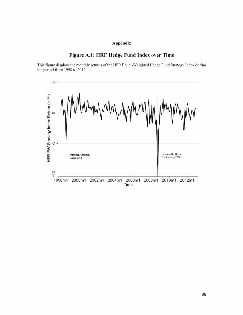
36  

Appendix

Figure A.1: HRF Hedge Fund Index over Time

This figure displays the monthly returns of the HFR Equal-Weighted Hedge Fund Strategy Index during the period from 1998 to 2012.

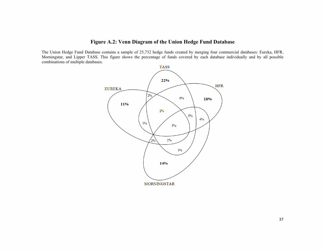
37  

Figure A.2: Venn Diagram of the Union Hedge Fund Database

The Union Hedge Fund Database contains a sample of 25,732 hedge funds created by merging four commercial databases: Eureka, HFR, Morningstar, and Lipper TASS. This figure shows the percentage of funds covered by each database individually and by all possible combinations of multiple databases.

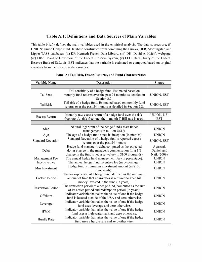
38  

Table A.1: Definitions and Data Sources of Main Variables

This table briefly defines the main variables used in the empirical analysis. The data sources are; (i) UNION: Union Hedge Fund Database constructed from combining the Eureka, HFR, Morningstar, and Lipper TASS databases, (ii) KF: Kenneth French Data Library, (iii) DH: David A. Hsieh's webpage, (iv) FRS: Board of Governors of the Federal Reserve System, (v) FED: Data library of the Federal Reserve Bank of St.Louis. EST indicates that the variable is estimated or computed based on original variables from the respective data sources.

Panel A: Tail Risk, Excess Returns, and Fund Characteristics

Variable Name Description Source

TailSens Tail sensitivity of a hedge fund. Estimated based on

monthly fund returns over the past 24 months as detailed in Section 2.2.

UNION, EST

TailRisk Tail risk of a hedge fund. Estimated based on monthly fund returns over the past 24 months as detailed in Section 2.2.

UNION, EST

Excess Return Monthly raw excess return of a hedge fund over the risk-

free rate. As risk-free rate, the 1-month T-Bill rate is used. UNION, KF,

EST

Size Natural logarithm of the hedge fund's asset under

management (in million USD). UNION

Age The age of a hedge fund since its inception (in months). UNION

Standard Deviation Standard Deviation of a hedge fund’s reported excess

returns over the past 24 months UNION, EST

Delta Hedge fund manager’s delta computed as the expected dollar change in the manager's compensation for a 1%

change in the fund’s net asset value (in $100 thousands)

Agarwal, Daniel, and Naik (2009)

Management Fee The annual hedge fund management fee (in percentage). UNION Incentive Fee The annual hedge fund incentive fee (in percentage). UNION

Min Investment Hedge fund’s minimum investment amount (in $100

thousands). UNION

Lockup Period The lockup period of a hedge fund, defined as the minimum

amount of time that an investor is required to keep his money invested in the fund (in years).

UNION

Restriction Period The restriction period of a hedge fund, computed as the sum

of its notice period and redemption period (in years). UNION

Offshore Indicator variable that takes the value of one if the hedge fund is located outside of the USA and zero otherwise.

UNION

Leverage Indicator variable that takes the value of one if the hedge

fund uses leverage and zero otherwise. UNION

HWM Indicator variable that takes the value of one if the hedge

fund uses a high-watermark and zero otherwise. UNION

Hurdle Rate Indicator variable that takes the value of one if the hedge

fund uses a hurdle rate and zero otherwise. UNION

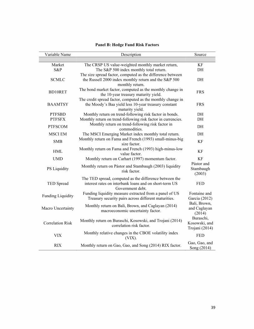
39  

Panel B: Hedge Fund Risk Factors

Variable Name Description Source

Market The CRSP US value-weighted monthly market return, KF S&P The S&P 500 index monthly total return. DH

SCMLC The size spread factor, computed as the difference between

the Russell 2000 index monthly return and the S&P 500 monthly return.

DH

BD10RET The bond market factor, computed as the monthly change in

the 10-year treasury maturity yield. FRS

BAAMTSY The credit spread factor, computed as the monthly change in

the Moody’s Baa yield less 10-year treasury constant maturity yield.

FRS

PTFSBD Monthly return on trend-following risk factor in bonds. DH PTFSFX Monthly return on trend-following risk factor in currencies. DH

PTFSCOM Monthly return on trend-following risk factor in

commodities. DH

MSCI EM The MSCI Emerging Market index monthly total return. DH

SMB Monthly return on Fama and French (1993) small-minus-big

size factor. KF

HML Monthly return on Fama and French (1993) high-minus-low

value factor. KF

UMD Monthly return on Carhart (1997) momentum factor. KF

PS Liquidity Monthly return on Pástor and Stambaugh (2003) liquidity

risk factor.

Pástor and Stambaugh

(2003)

TED Spread The TED spread, computed as the difference between the

interest rates on interbank loans and on short-term US Government debt.

FED

Funding Liquidity Funding liquidity measure extracted from a panel of US

Treasury security pairs across different maturities. Fontaine and Garcia (2012)

Macro Uncertainty Monthly return on Bali, Brown, and Caglayan (2014)

macroeconomic uncertainty factor.

Bali, Brown, and Caglayan

(2014)

Correlation Risk Monthly return on Buraschi, Kosowski, and Trojani (2014)

correlation risk factor.

Buraschi, Kosowski, and Trojani (2014)

VIX Monthly relative changes in the CBOE volatility index

(VIX). FED

RIX Monthly return on Gao, Gao, and Song (2014) RIX factor. Gao, Gao, and Song (2014)

40  

References

Agarwal, Vikas, and Narayan Y. Naik, 2004, Risks and portfolio decisions involving hedge

funds, Review of Financial Studies 17, 63–98.

Agarwal, Vikas, Gurdip Bakshi, and Joop Huij, 2009, Do higher-moment equity risks explain

hedge fund returns? Working Paper, Erasmus University, Georgia State University, and

University of Maryland.

Agarwal, Vikas, Naveen D. Daniel, and Narayan Y. Naik, 2003, Flows, performance, and

managerial incentives in the hedge fund industry, Working Paper, Georgia State University

and London Business School.

Agarwal, Vikas, Naveen D. Daniel, and Narayan Y. Naik, 2009, Role of managerial incentives

and discretion in hedge fund performance, Journal of Finance 64, 22212256.

Agarwal, Vikas, Vyacheslav Fos, and Wei Jiang, 2013, Inferring reporting-related biases in

hedge fund databases from hedge fund equity holdings, Management Science 59,

12711289.

Agarwal, Vikas, Wei Jiang, Yuehua Tang, and Baozhong Yang, 2013, Uncovering hedge fund

skill from the portfolios they hide, Journal of Finance 68, 739783.

Ang, Andrew, Joseph Chen, and Yuhang Xing, 2006, Downside risk, Review of Financial

Studies 19, 1191239.

Aragon, George O., 2007, Share restrictions and asset pricing: Evidence from the hedge fund

industry, Journal of Financial Economics 83, 33–58.

Aragon, George O., and J. Spencer Martin, 2012, A unique view of hedge fund derivatives

usage: Safeguard or speculation? Journal of Financial Economics 105, 436–456.

Aragon, George O., and Vikram Nanda, 2012, Tournament behavior in hedge funds: High-

water marks, fund liquidation, and managerial stake, Review of Financial Studies 25,

937974.

Aragon, George O., and Philip E. Strahan, 2012, Hedge funds as liquidity providers: Evidence

from the Lehman bankruptcy, Journal of Financial Economics 103, 570587.

Bali, Turan G., Suleyman Gokcan, and Bing Liang, 2007, Value at risk and the cross-section

of hedge fund returns, Journal of Banking and Finance, 31, 11351166.

41  

Bali, Turan G., Stephen J. Brown, and Mustafa O. Caglayan, 2014, Macroeconomic risk and

hedge fund returns, Journal of Financial Economics, 114, 119.

Bondarenko, Oleg, 2004, Market price of variance risk and performance of hedge funds,

Working Paper, University of Illinois.

Boyson, Nicole M., Christof W. Stahel, and René M. Stulz, 2010, Hedge fund contagion and

liquidity shocks, Journal of Finance, 65, 17891816.

Brown, Stephen J., and Jonathan F. Spitzer, 2006, Caught by the tail: Tail risk neutrality and

hedge fund returns, Working Paper, New York University.

Brown, Stephen J., William N. Goetzmann, and James Park, 2001, Careers and survival:

competition and risk in the hedge fund and CTA industry, Journal of Finance 56,

18691886.

Brown, Stephen J., Greg N. Gregoriou, and Razvan Pascalau, 2012, Is it possible to

overdiversify? The case of funds of hedge funds, Review of Asset Pricing Studies 2,

89110.

Buraschi, Andrea, Robert Kosowski, and Fabio Trojani, 2014, When there is no place to hide:

correlation risk and the cross-section of hedge fund returns, Review of Financial Studies

27, 581–616.

Cao, Charles, Yong Chen, Bing Liang, and Andrew W. Lo, 2013, Can hedge funds fund time

market liquidity? Journal of Financial Economics 109, 493–516.

Carhart, Mark, 1997, On Persistence in Mutual Fund Performance, Journal of Finance 52, 57–

82.

Chabi-Yo, Fousseni, Stefan Ruenzi, and Florian Weigert, 2015, Crash sensitivity and the cross-

section of expected stock returns, Working Paper, Ohio State University, University of

Mannheim, and University of St. Gallen.

Chen, Yong, 2007, Timing ability in the focus market of hedge funds, Journal of Investment

Management 5, 66–98.

Chen, Yong, and Bing Liang, 2007, Do market timing hedge funds time the market? Journal

of Financial and Quantitative Analysis 42, 827–856.

Duarte, Jefferson, Francis Longstaff, and Fan Yu, 2007, Risk and return in fixed income

arbitrage: nickels in front of a steamroller? Review of Financial Studies 20, 769811.

42  

Fama, Eugene F., and Kenneth R. French, 1993, Common risk factors in the returns on stocks

and bonds, Journal of Financial Economics 33, 356.

Fama, Eugene F., and James D. MacBeth, 1973, Risk, return, and equilibrium: empirical tests,

Journal of Political Economy 81, 607636.

Farnsworth, Grant, 2014, Strategic hedge fund leverage and investor welfare: A holdings-based

approach, Working Paper, Penn State University.

Fontaine, Jean-Sébastien, and René Garcia, 2012, Bond Liquidity Premia, Review of Financial

Studies 25, 1207–1254.

Fung, William, and David A. Hsieh, 1997, Empirical characteristics of dynamic trading

strategies: The case of hedge funds, Review of Financial Studies 10, 275–302.

Fung, William, and David A. Hsieh, 2001, The risk in hedge fund strategies: theory and

evidence from trend followers, Review of Financial Studies 14, 313–341.

Fung, William, and David A. Hsieh, 2004, Hedge fund benchmarks: A risk-based approach,

Financial Analysts Journal 60, 65–80.

Gao, George P., Pengjie Gao, and Zhaogang Song, 2014, Do hedge funds exploit rare disaster

concerns?, Working Paper, Cornell University and the University of Notre Dame.

Getmansky, Mila, Andrew W. Lo, and Igor Makarow, 2004. An Econometric Model of Serial

Correlation and Illiquidity in Hedge Fund Returns, Journal of Financial Economics 74,

319352.

Goetzmann, William N., Jonathan E. Ingersoll, and Stephen A. Ross, 2003, High-water marks

and hedge fund management contracts, Journal of Finance 58, 16851717.

Goetzmann, William N., Jonathan E. Ingersoll, Matthew Spiegel, and Ivo Welch, 2007,

Portfolio performance manipulation and manipulation-proof performance measures,

Review of Financial Studies 58, 15031546.

Graham, John R., and Campbell R. Harvey, 1996, Market timing ability and volatility implied

in investment newsletters’ asset allocation recommendations, Journal of Financial

Economics 42, 397–422.

Graham, John R., and Campbell R. Harvey, 1997, Grading the performance of market-timing

newsletters, Financial Analysts Journal 53, 54–66.

43  

Griffin, John M., and Jin Xu, 2009, How smart are the smart guys? A unique view from hedge

fund stock holdings, Review of Financial Studies 22, 23312370.

Hodder, James E., and Jens C. Jackwerth, 2007, Incentive contracts and hedge fund

management, Journal of Financial and Quantitative Analysis 42, 811826.

Hodder, James E., Jens C. Jackwerth, and Olga Kolokolova, 2014, Recovering Delisting

Returns of Hedge Funds, Journal of Financial and Quantitative Analysis 49, 797815.

Jiang, Hao, and Bryan Kelly, 2012, Tail risk and hedge fund returns, Working Paper, Erasmus

University Rotterdam and University of Chicago Booth School of Business.

Kelly, Bryan, and Hao Jiang, 2014, Tail risk and asset prices, Review of Financial Studies 27,

28412871.

Kolokolova, Olga, and Achim Mattes, 2014, Recovering Managerial Risk Taking from Daily

Hedge Fund Returns: Incentives at Work? University of Manchester and University of

Konstanz.

Kosowski, Robert, Narayan Y. Naik, and Melvyn Teo, 2007, Do hedge funds deliver alpha? A

Bayesian and bootstrap analysis, Journal of Financial Economics 84, 229‒264.

Liang, Bing, and Hyuna Park, 2007, Risk measures for hedge funds: a cross-sectional approach,

European Financial Management 13, 333370.

Liang, Bing, and Hyuna Park, 2010, Predicting hedge fund failure: A comparison of risk

measures, Journal of Financial and Quantitative Analysis 45, 199222.

Longin, Francois, and Bruno Solnik, 2001, Extreme correlation of international equity markets,

Journal of Finance 56, 649676.

Mitchell, Mark, and Todd Pulvino, 2001, Characteristics of risk and return in risk arbitrage,

Journal of Finance 56, 2135–2175.

Modigliani, Franco, and Leah Modigliani, 1997, Risk-adjusted performance, Journal of

Portfolio Management 23, 45–54.

Newey, Whitney K., and Kenneth D. West, 1987, A simple, positive semi-definite,

heteroskedasticity and autocorrelation consistent covariance matrix, Econometrica 55,

703–708.

44  

Ozik, Gideon, and Ronnie Sadka, 2015, Skin in the game versus skimming the game:

governance, share restrictions, and insider flow, Journal of Financial and Quantitative

Analysis, forthcoming.

Panageas, Stavros, and Mark Westerfield, 2009, High-water marks: High-risk appetites?

Convex compensation, long horizons, and portfolio choice, Journal of Finance 64, 136.

Pástor, Ľuboš, and Robert Stambaugh, 2003, Liquidity risk and expected stock returns, Journal

of Political Economy 111, 642–685.

Rodriguez, Juan C., 2007, Measuring financial contagion: A copula approach, Journal of

Empirical Finance 14, 401423.

Sadka, Ronnie, 2010, Liquidity risk and the cross-section of hedge fund returns, Journal of

Financial Economics 98, 54–71.

Shanken, Jay, 1992, On the estimation of beta-pricing models, Review of Financial Studies 5,

1–33.

Stulz, René, 2007, Hedge funds: past, present, and future, Journal of Economic Perspectives

21, 175–194.

Teo, Melvyn, 2011, The liquidity risk of liquid hedge funds, Journal of Financial Economics

100, 24–44.

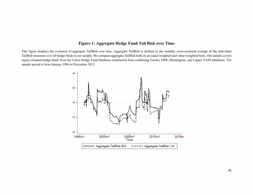
45  

Figure 1: Aggregate Hedge Fund Tail Risk over Time

This figure displays the evolution of aggregate TailRisk over time. Aggregate TailRisk is defined as the monthly cross-sectional average of the individual TailRisk measures over all hedge funds in our sample. We compute aggregate TailRisk both on an equal-weighted and value-weighted basis. Our sample covers equity-oriented hedge funds from the Union Hedge Fund Database constructed from combining Eureka, HFR, Morningstar, and Lipper TASS databases. The sample period is from January 1996 to December 2012.

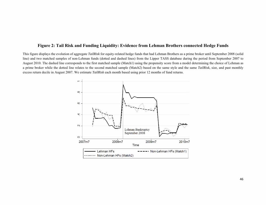
46  

Figure 2: Tail Risk and Funding Liquidity: Evidence from Lehman Brothers connected Hedge Funds

This figure displays the evolution of aggregate TailRisk for equity-related hedge funds that had Lehman Brothers as a prime broker until September 2008 (solid line) and two matched samples of non-Lehman funds (dotted and dashed lines) from the Lipper TASS database during the period from September 2007 to August 2010. The dashed line corresponds to the first matched sample (Match1) using the propensity score from a model determining the choice of Lehman as a prime broker while the dotted line relates to the second matched sample (Match2) based on the same style and the same TailRisk, size, and past monthly excess return decile in August 2007. We estimate TailRisk each month based using prior 12 months of fund returns.

47  

Figure 3: Tail Risk Timing: Evidence From Equity Holdings in the Financial Crisis 2008

This figure displays the evolution of aggregate actual TailRisk of hedge fund firms’ disclosed long equity holdings (dashed line) and the evolution of aggregate hypothetical TailRisk based on hedge funds firms’ disclosed long equity holdings from March 2008 (solid line) during the period from March 2008 to March 2009. We estimate TailRisk each month based using prior 24 months of returns. Our sample covers hedge fund firms from the Union Hedge Fund Database constructed from combining Eureka, HFR, Morningstar, and Lipper TASS databases who report 13F long equity holdings to the SEC.

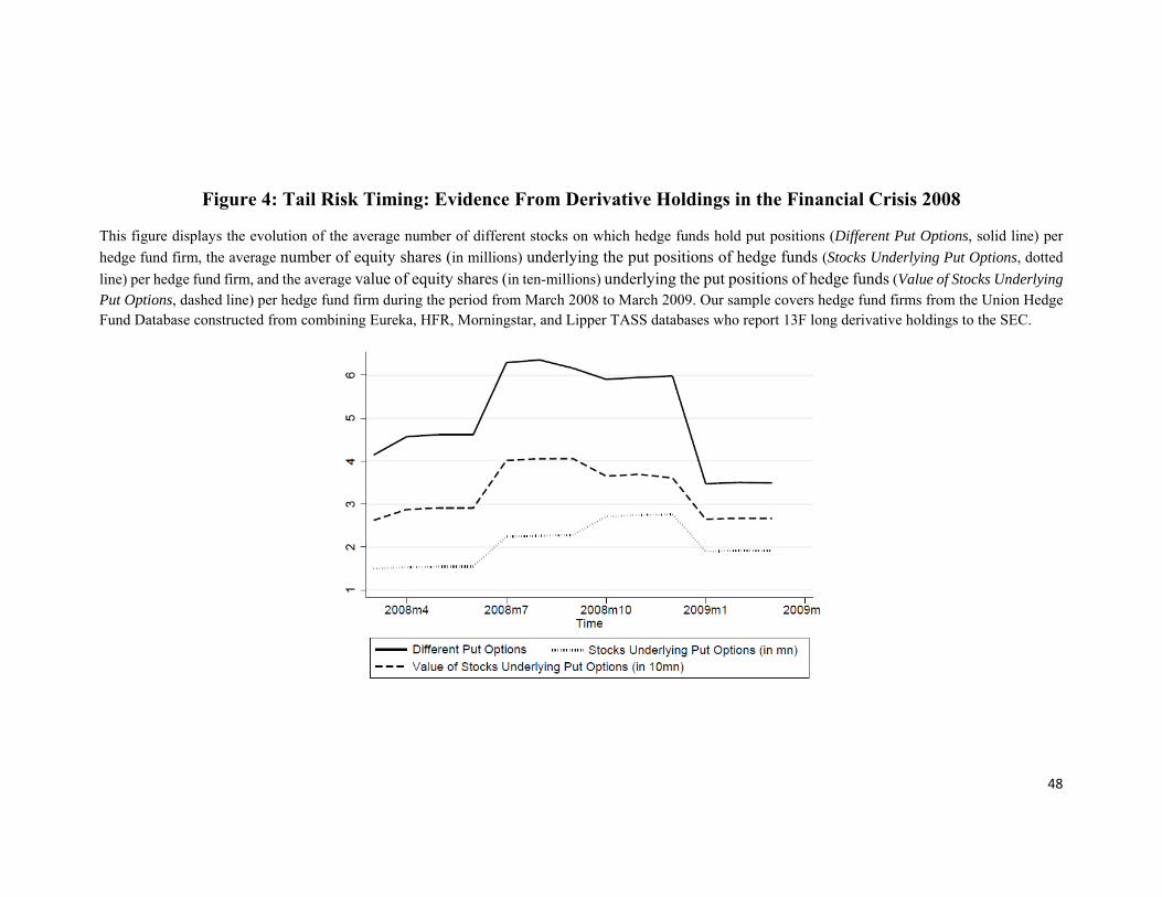
48  

Figure 4: Tail Risk Timing: Evidence From Derivative Holdings in the Financial Crisis 2008

This figure displays the evolution of the average number of different stocks on which hedge funds hold put positions (Different Put Options, solid line) per

hedge fund firm, the average number of equity shares (in millions) underlying the put positions of hedge funds (Stocks Underlying Put Options, dotted

line) per hedge fund firm, and the average value of equity shares (in ten-millions) underlying the put positions of hedge funds (Value of Stocks Underlying Put Options, dashed line) per hedge fund firm during the period from March 2008 to March 2009. Our sample covers hedge fund firms from the Union Hedge Fund Database constructed from combining Eureka, HFR, Morningstar, and Lipper TASS databases who report 13F long derivative holdings to the SEC.

49  

Table 1: Summary Statistics

This table provides summary statistics for the monthly excess returns (over the risk-free rate) of hedge funds (Panel A), fund characteristics (Panel B), the and the TailRisk measure as defined in equation (2) in the main text (Panel C). Summary statistics are calculated over all hedge funds and months in our sample period. As the risk-free rate we use the one-month T-bill rate. We also display correlations between TailRisk and fund characteristics in Panel D. Finally, we provide correlations between the aggregate TailRisk measure (computed as the equal-weighted average over all hedge funds) with various risk factors (as defined in the paper) in Panel E. Our sample covers hedge funds from the Union Hedge Fund Database constructed from combining the Eureka, HFR, Morningstar, and Lipper TASS databases. The sample period is from January 1996 to December 2012. All variables are defined in Table A.1.

Panel A: Excess Returns Sample Mean 25% Median 75% StdDev

All 0.52% ‒0.98% 0.42% 1.89% 5.23

Panel B: Fund Characteristics Variable Mean 25% Median 75% StdDev

Size 3.35 2.19 3.40 4.56 1.83 Age (in months) 63.85 22.00 48.00 90.00 55.86

Standard Deviation 4.54 2.09 3.53 5.81 3.81 Delta (in $100 thousands) 1.83 0.07 0.37 1.46 4.16 Management Fee (in %) 1.41 1.00 1.50 1.75 0.53

Incentive Fee (in %) 18.13 20.00 20.00 20.00 5.56 Min Investment (in $100 thousands) 10.90 1.50 5.00 10.00 92.81

Lockup Period (in years) 0.41 0.00 0.00 1.00 0.61Restriction Period (in years) 0.34 0.16 0.33 0.38 0.30

Offshore 0.51 0.00 1.00 1.00 0.50 Leverage 0.60 0.00 1.00 1.00 0.49

HWM 0.80 1.00 1.00 1.00 0.40 Hurdle Rate 0.27 0.00 0.00 1.00 0.44

50  

Panel C: TailRisk

Strategy Number of Funds Avg TailRisk 10% 25% Median 75% 90% Std Dev Emerging Markets 531 0.51 0.00 0.00 0.26 0.81 1.36 0.71

Event Driven 852 0.25 0.00 0.00 0.04 0.35 0.66 0.42 Equity Long-Short 3736 0.41 0.00 0.00 0.21 0.64 1.10 0.58 Equity Long Only 331 0.49 0.00 0.00 0.30 0.76 1.24 0.68

Equity Market Neutral 1,265 0.12 0.00 0.00 0.00 0.10 0.39 0.29 Short Bias 66 0.07 0.00 0.00 0.00 0.00 0.12 0.27

Sector 250 0.49 0.00 0.00 0.26 0.75 1.30 0.70 All 6,281 0.38 0.00 0.00 0.12 0.58 1.06 0.58

Panel D: Correlation between TailRisk and Fund Characteristics

TailRisk Size Age Standard Deviation

Delta Management

Fee Incentive

Fee Min

Investment Lockup Period

Restriction Period

Offshore Leverage HWM Hurdle Rate

TailRisk 1.00 Size ‒0.09 1.00 Age 0.05 0.26 1.00

Std. Dev. 0.29 ‒0.22 ‒0.03 1.00 Delta 0.08 0.49 0.28 ‒0.09 1.00

Mgmt. Fee ‒0.00 0.07 ‒0.07 0.03 0.05 1.00 Inc. Fee ‒0.02 0.00 ‒0.09 ‒0.02 0.10 ‒0.03 1.00 Min Inv ‒0.05 0.26 0.06 ‒0.09 0.27 ‒0.03 0.01 1.00 Lockup 0.07 0.00 0.01 0.05 ‒0.00 ‒0.04 0.13 0.05 1.00

Restriction ‒0.00 0.10 0.08 ‒0.02 0.12 ‒0.11 0.14 0.07 0.30 1.00 Offshore ‒0.01 0.15 ‒0.09 ‒0.00 0.08 0.22 ‒0.04 ‒0.08 ‒0.24 ‒0.30 1.00 Leverage 0.09 0.03 ‒0.01 0.02 0.03 0.03 0.14 ‒0.03 0.04 0.03 0.03 1.00

HWM 0.00 0.05 ‒0.06 ‒0.01 0.07 0.07 0.30 0.02 0.14 0.07 ‒0.04 0.09 1.00 Hurdle Rate ‒0.01 ‒0.05 0.11 ‒0.01 ‒0.03 ‒0.13 0.02 0.03 0.11 0.17 ‒0.47 0.03 ‒0.09 1.00

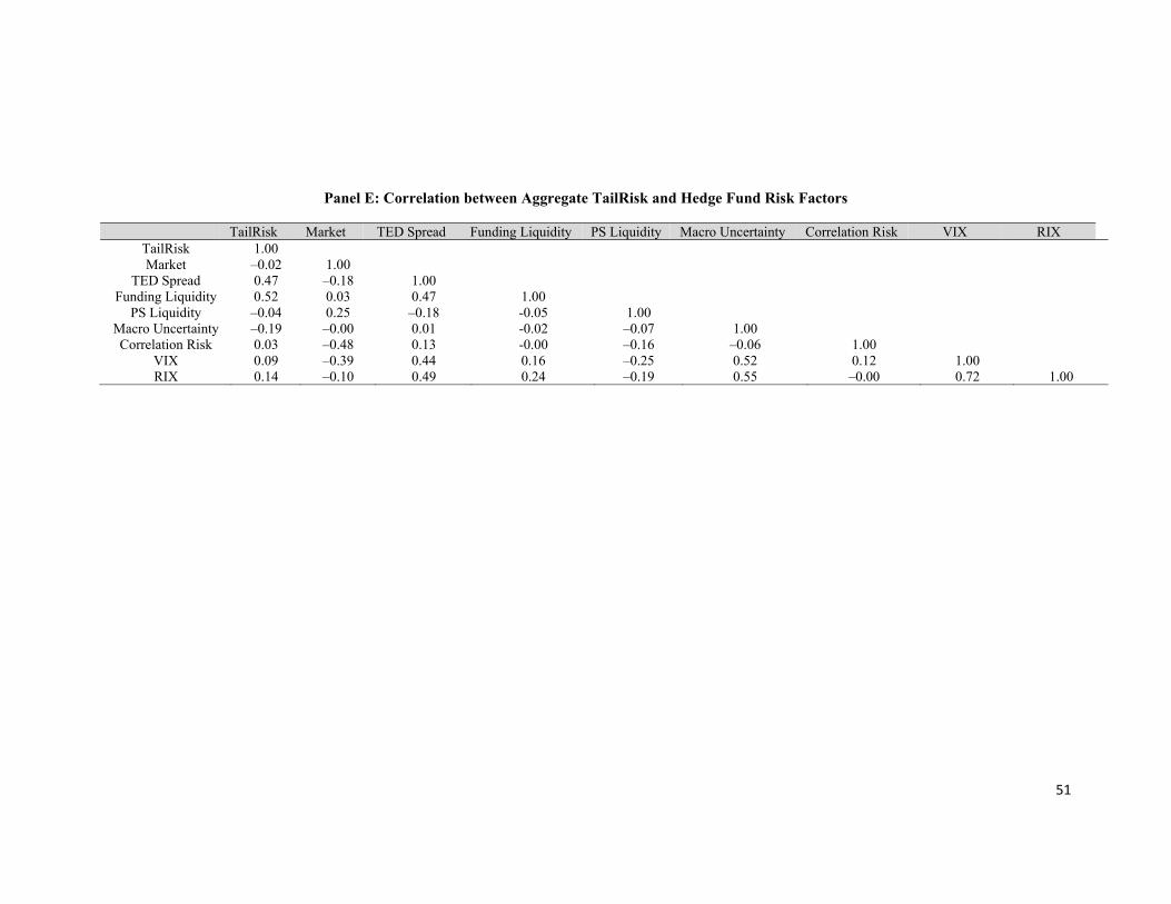
51  

Panel E: Correlation between Aggregate TailRisk and Hedge Fund Risk Factors

TailRisk Market TED Spread Funding Liquidity PS Liquidity Macro Uncertainty Correlation Risk VIX RIX TailRisk 1.00 Market ‒0.02 1.00

TED Spread 0.47 ‒0.18 1.00 Funding Liquidity 0.52 0.03 0.47 1.00

PS Liquidity ‒0.04 0.25 ‒0.18 -0.05 1.00 Macro Uncertainty ‒0.19 ‒0.00 0.01 -0.02 ‒0.07 1.00 Correlation Risk 0.03 ‒0.48 0.13 -0.00 ‒0.16 ‒0.06 1.00

VIX 0.09 ‒0.39 0.44 0.16 ‒0.25 0.52 0.12 1.00 RIX 0.14 ‒0.10 0.49 0.24 ‒0.19 0.55 ‒0.00 0.72 1.00

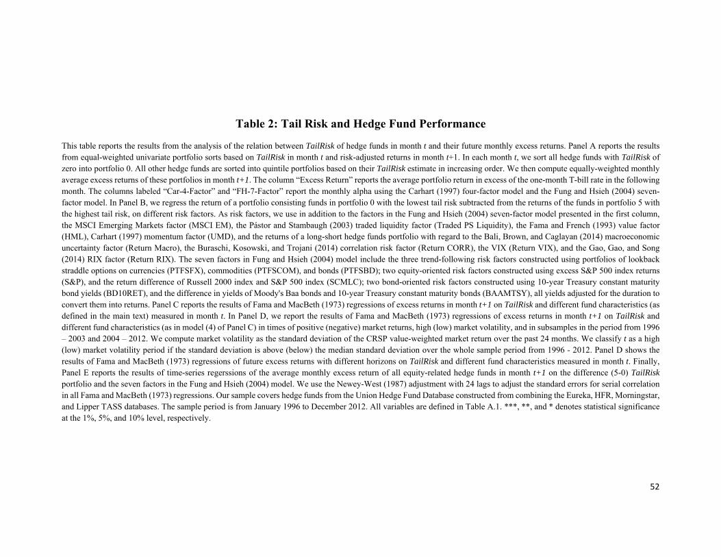
52  

Table 2: Tail Risk and Hedge Fund Performance

This table reports the results from the analysis of the relation between TailRisk of hedge funds in month t and their future monthly excess returns. Panel A reports the results from equal-weighted univariate portfolio sorts based on TailRisk in month t and risk-adjusted returns in month t+1. In each month t, we sort all hedge funds with TailRisk of zero into portfolio 0. All other hedge funds are sorted into quintile portfolios based on their TailRisk estimate in increasing order. We then compute equally-weighted monthly average excess returns of these portfolios in month t+1. The column “Excess Return” reports the average portfolio return in excess of the one-month T-bill rate in the following month. The columns labeled “Car-4-Factor” and “FH-7-Factor” report the monthly alpha using the Carhart (1997) four-factor model and the Fung and Hsieh (2004) seven-factor model. In Panel B, we regress the return of a portfolio consisting funds in portfolio 0 with the lowest tail risk subtracted from the returns of the funds in portfolio 5 with the highest tail risk, on different risk factors. As risk factors, we use in addition to the factors in the Fung and Hsieh (2004) seven-factor model presented in the first column, the MSCI Emerging Markets factor (MSCI EM), the Pástor and Stambaugh (2003) traded liquidity factor (Traded PS Liquidity), the Fama and French (1993) value factor (HML), Carhart (1997) momentum factor (UMD), and the returns of a long-short hedge funds portfolio with regard to the Bali, Brown, and Caglayan (2014) macroeconomic uncertainty factor (Return Macro), the Buraschi, Kosowski, and Trojani (2014) correlation risk factor (Return CORR), the VIX (Return VIX), and the Gao, Gao, and Song (2014) RIX factor (Return RIX). The seven factors in Fung and Hsieh (2004) model include the three trend-following risk factors constructed using portfolios of lookback straddle options on currencies (PTFSFX), commodities (PTFSCOM), and bonds (PTFSBD); two equity-oriented risk factors constructed using excess S&P 500 index returns (S&P), and the return difference of Russell 2000 index and S&P 500 index (SCMLC); two bond-oriented risk factors constructed using 10-year Treasury constant maturity bond yields (BD10RET), and the difference in yields of Moody's Baa bonds and 10-year Treasury constant maturity bonds (BAAMTSY), all yields adjusted for the duration to convert them into returns. Panel C reports the results of Fama and MacBeth (1973) regressions of excess returns in month t+1 on TailRisk and different fund characteristics (as defined in the main text) measured in month t. In Panel D, we report the results of Fama and MacBeth (1973) regressions of excess returns in month t+1 on TailRisk and different fund characteristics (as in model (4) of Panel C) in times of positive (negative) market returns, high (low) market volatility, and in subsamples in the period from 1996 ‒ 2003 and 2004 ‒ 2012. We compute market volatility as the standard deviation of the CRSP value-weighted market return over the past 24 months. We classify t as a high (low) market volatility period if the standard deviation is above (below) the median standard deviation over the whole sample period from 1996 - 2012. Panel D shows the results of Fama and MacBeth (1973) regressions of future excess returns with different horizons on TailRisk and different fund characteristics measured in month t. Finally, Panel E reports the results of time-series regerssions of the average monthly excess return of all equity-related hedge funds in month t+1 on the difference (5-0) TailRisk portfolio and the seven factors in the Fung and Hsieh (2004) model. We use the Newey-West (1987) adjustment with 24 lags to adjust the standard errors for serial correlation in all Fama and MacBeth (1973) regressions. Our sample covers hedge funds from the Union Hedge Fund Database constructed from combining the Eureka, HFR, Morningstar, and Lipper TASS databases. The sample period is from January 1996 to December 2012. All variables are defined in Table A.1. ***, **, and * denotes statistical significance at the 1%, 5%, and 10% level, respectively.

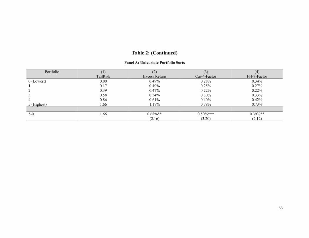
53  

Table 2: (Continued)

Panel A: Univariate Portfolio Sorts

Portfolio (1) TailRisk

(2) Excess Return

(3) Car-4-Factor

(4) FH-7-Factor

0 (Lowest) 0.00 0.49% 0.28% 0.34% 1 0.17 0.40% 0.25% 0.27% 2 0.39 0.47% 0.22% 0.22% 3 0.58 0.54% 0.30% 0.33% 4 0.86 0.61% 0.40% 0.42% 5 (Highest) 1.66 1.17% 0.78% 0.73% 5-0 1.66 0.68%**

(2.16) 0.50%***

(3.20) 0.39%**

(2.12)

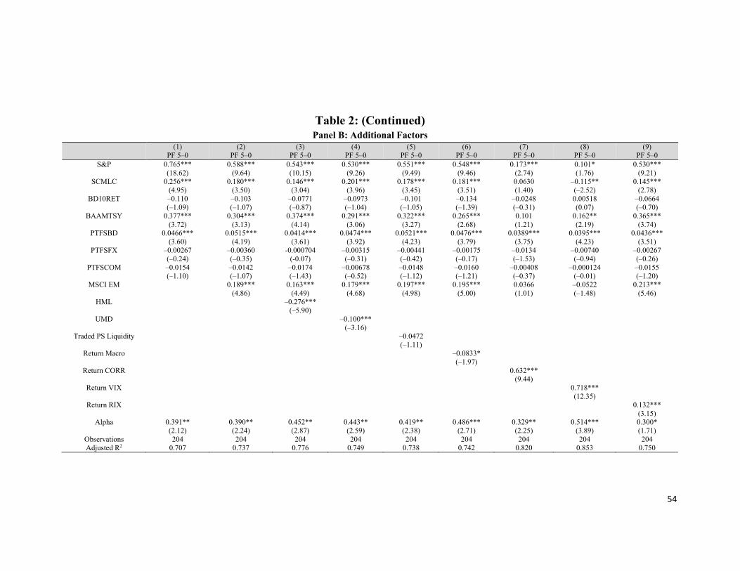
54  

Table 2: (Continued) Panel B: Additional Factors

(1) PF 5‒0

(2) PF 5‒0

(3) PF 5‒0

(4) PF 5‒0

(5) PF 5‒0

(6) PF 5‒0

(7) PF 5‒0

(8) PF 5‒0

(9) PF 5‒0

S&P 0.765*** (18.62)

0.588*** (9.64)

0.543*** (10.15)

0.530*** (9.26)

0.551*** (9.49)

0.548*** (9.46)

0.173*** (2.74)

0.101* (1.76)

0.530*** (9.21)

SCMLC 0.256*** (4.95)

0.180*** (3.50)

0.146*** (3.04)

0.201*** (3.96)

0.178*** (3.45)

0.181*** (3.51)

0.0630 (1.40)

‒0.115** (‒2.52)

0.145*** (2.78)

BD10RET ‒0.110 (‒1.09)

‒0.103 (‒1.07)

‒0.0771 (‒0.87)

‒0.0973 (‒1.04)

‒0.101 (‒1.05)

‒0.134 (‒1.39)

‒0.0248 (‒0.31)

0.00518 (0.07)

‒0.0664 (‒0.70)

BAAMTSY 0.377*** (3.72)

0.304*** (3.13)

0.374*** (4.14)

0.291*** (3.06)

0.322*** (3.27)

0.265*** (2.68)

0.101 (1.21)

0.162** (2.19)

0.365*** (3.74)

PTFSBD 0.0466*** (3.60)

0.0515*** (4.19)

0.0414*** (3.61)

0.0474*** (3.92)

0.0521*** (4.23)

0.0476*** (3.79)

0.0389*** (3.75)

0.0395*** (4.23)

0.0436*** (3.51)

PTFSFX ‒0.00267 (‒0.24)

‒0.00360 (‒0.35)

-0.000704 (-0.07)

‒0.00315 (‒0.31)

‒0.00441 (‒0.42)

‒0.00175 (‒0.17)

‒0.0134 (‒1.53)

‒0.00740 (‒0.94)

‒0.00267 (‒0.26)

PTFSCOM ‒0.0154 (‒1.10)

‒0.0142 (‒1.07)

‒0.0174 (‒1.43)

‒0.00678 (‒0.52)

‒0.0148 (‒1.12)

‒0.0160 (‒1.21)

‒0.00408 (‒0.37)

‒0.000124 (‒0.01)

‒0.0155 (‒1.20)

MSCI EM

0.189*** (4.86)

0.163*** (4.49)

0.179*** (4.68)

0.197*** (4.98)

0.195*** (5.00)

0.0366 (1.01)

‒0.0522 (‒1.48)

0.213*** (5.46)

HML

‒0.276*** (‒5.90)

UMD

‒0.100*** (‒3.16)

Traded PS Liquidity ‒0.0472 (‒1.11)

Return Macro ‒0.0833* (‒1.97)

Return CORR 0.632*** (9.44)

Return VIX 0.718*** (12.35)

Return RIX 0.132*** (3.15)

Alpha

0.391** (2.12)

0.390** (2.24)

0.452** (2.87)

0.443** (2.59)

0.419** (2.38)

0.486*** (2.71)

0.329** (2.25)

0.514*** (3.89)

0.300* (1.71)

Observations 204 204 204 204 204 204 204 204 204 Adjusted R2 0.707 0.737 0.776 0.749 0.738 0.742 0.820 0.853 0.750

55  

Table 2: (Continued)

Panel C: Fama and MacBeth Regressions (1)

Future Excess Return

(2) Future Excess

Return

(3) Future Excess

Return

(4) Future Excess

Return TailRisk 0.451**

(2.01) 0.306** (2.34)

0.240*** (2.60)

0.227*** (3.16)

Size ‒0.0906*** (‒3.16)

‒0.0848*** (‒3.28)

Age ‒0.000107 (‒0.26)

‒0.000203 (‒0.50)

Delta 0.0190*** (2.86)

0.0168*** (3.12)

Management Fee 0.0488 (1.28)

0.0403 (1.05)

Incentive Fee ‒0.000903 (‒0.30)

‒0.0000219 (‒0.01)

Min Investment 0.00233** (2.54)

0.00207*** (2.97)

Lockup Period 0.0490 (1.49)

0.0556* (1.73)

Restriction Period 0.0721* (1.91)

0.0456 (1.24)

Offshore 0.0350 (0.47)

0.0308 (0.43)

Leverage 0.0268 (0.64)

0.0277 (0.71)

HWM 0.125** (2.50)

0.103** (2.21)

Hurdle Rate 0.108*** (3.99)

0.102*** (4.50)

Past Yearly Return 0.0221*** (7.36)

0.0229*** (9.42)

Standard Deviation 0.0182 (0.54)

0.0361 (0.98)

Skewness 0.154** (2.54)

0.0379 (1.04)

Kurtosis ‒0.0126 (‒0.62)

‒0.0178 (‒1.44)

VaR 0.00130 (0.06)

0.0150 (1.13)

Beta 0.262 (1.07)

0.112 (0.48)

Constant 0.426*** (3.08)

0.272** (2.11)

0.509*** (4.18)

0.352*** (2.61)

Observations 420,329 195,170 420,329 195,170 Adjusted R2 0.058 0.165 0.160 0.230

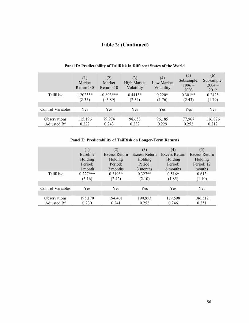
56  

Table 2: (Continued)

Panel D: Predictability of TailRisk in Different States of the World

(1)

Market Return > 0

(2) Market

Return < 0

(3) High Market

Volatility

(4) Low Market

Volatility

(5) Subsample:

1996 ‒ 2003

(6) Subsample:

2004 ‒ 2012

TailRisk 1.202*** (8.35)

‒0.893*** (‒5.89)

0.441** (2.54)

0.220* (1.76)

0.301** (2.43)

0.242* (1.79)

Control Variables Yes Yes Yes Yes Yes Yes

Observations 115,196 79,974 98,658 96,185 77,967 116,876 Adjusted R2 0.222 0.243 0.232 0.229 0.252 0.212

Panel E: Predictability of TailRisk on Longer-Term Returns

(1) Baseline Holding Period: 1 month

(2) Excess Return

Holding Period:

2 months

(3) Excess Return

Holding Period:

3 months

(4) Excess Return

Holding Period:

6 months

(5) Excess Return

Holding Period: 12

months TailRisk 0.227***

(3.16) 0.319** (2.42)

0.327** (2.10)

0.516* (1.85)

0.613 (1.10)

Control Variables Yes Yes Yes Yes Yes

Observations 195,170 194,401 190,953 189,598 186,512 Adjusted R2 0.230 0.241 0.252 0.246 0.251

57  

Table 2: (Continued)

Panel F: Time Series Regressions

Fung and Hsieh (2004) Model

Equity-Related

Emerging Markets

Event Driven Equity

Long-Short Equity

Long Only

Equity Market Neutral

Short Bias Sector

S&P 0.432*** (21.55)

0.241*** (7.79)

0.212*** (2.63)

0.174*** (7.55)

0.288*** (8.57)

0.318*** (5.79)

0.079*** (4.10)

‒0.471*** (‒7.36)

0.254*** (3.90)

SMB 0.275*** (10.91)

0.205*** (8.25)

0.124* (1.92)

0.140*** (7.57)

0.255*** (9.46)

0.177*** (4.01)

0.028* (1.79)

‒0.372*** (‒7.25)

0.385*** (7.38)

Term ‒0.082* (‒1.73)

‒0.076* (‒1.66)

‒0.102 (‒0.85)

‒0.069** (‒2.00)

‒0.0894* (‒1.80)

‒0.084 (‒1.02)

0.005 (0.17)

‒0.022 (‒0.24)

‒0.069 (‒0.71)

Credit 0.206***

(4.12) 0.120** (2.52)

0.309** (2.50)

0.268*** (7.58)

0.054 (1.05)

0.245*** (2.91)

0.077*** (2.61)

0.220** (2.24)

‒0.089 (‒0.88)

PTFSBD ‒0.007 (‒1.13)

‒0.019*** (‒3.10)

‒0.054*** (‒3.45)

‒0.021*** (‒4.67)

‒0.015** (‒2.24)

‒0.013 (‒1.20)

‒0.007* (‒1.97)

‒0.008 (‒0.67)

‒0.010 (‒0.77)

PTFSFX 0.008* (1.68)

0.010** (2.01)

0.021 (1.61)

0.007* (1.81)

0.010* (1.92)

0.004 (0.47)

0.005* (1.66)

0.002 (0.23)

0.012 (1.13)

PTFSCOM 0.000 (0.04)

0.003 (0.45)

0.003 (0.20)

‒0.004 (‒0.74)

0.004 (0.62)

0.002 (0.17)

0.000 (0.05)

‒0.004 (-0.28)

0.012 (0.87)

TailRisk 10 ‒ 1 0.244***

(7.56) 0.486***

(5.77) 0.083***

(3.46) 0.259***

(7.38) 0.313***

(5.45) ‒0.007 (‒0.35)

‒0.234*** (‒3.50)

0.501*** (7.37)

Constant 0.436***

(5.04) 0.353***

(4.18) 0.275 (1.25)

0.395*** (6.29)

0.366*** (4.01)

0.331** (2.21)

0.355*** (6.81)

0.295* (1.70)

0.347* (1.95)

Difference to Constant in FH-7-Factor Model

‒

‒0.083 ‒0.104 ‒0.032 ‒0.090 ‒0.045 +0.007 +0.015 ‒0.260

Adjusted R2 0.778 0.830 0.599 0.796 0.834 0.712 0.263 0.669 0.713

Improvement in Adjusted R2 in

Comparison to FH-7-Factor Model

‒

0.052 (6.68%)

0.100 (20.04%)

0.031 (4.05%)

0.047 (5.97%)

0.057 (8.70%)

‒0.006 (‒2.22%)

0.037 (5.85%)

0.086 (13.72%)

58  

Table 3: Tail Risk and Hedge Fund Performance: Robustness Checks

This table reports the results from robustness checks of the relation between TailRisk of hedge funds in month t and their monthly excess returns in month t+1. We investigate the robustness if we (i) change the estimation horizon of the TailRisk measure to 3 and 4 years, respectively, (ii) compute TailRisk using different cut-off values of 10% and 20% to define worst returns, (iii) use VaR instead of ES in the computation of TailRisk, (iv) apply a value-weighted sorting procedure instead of an equal-weighted sorting procedure, and (v) assign a delisting return of -20% to those hedge funds that leave the database. Moreover, we check the robustness if we use returns reported after the listing date for funds in the Lipper TASS database. Panel A displays the results of from the same univariate portfolio sorts as in Column 4, Panel A, Table 2 using these alternative definitions of TailRisk. Panel B reports the results of Fama and MacBeth (1973) regression (4) of Panel C in Table 2 of future excess returns in month t+1 on the same alternative TailRisk definitions and different fund characteristics measured in month t. The baseline specification in Column (1) is to estimate TailRisk as in Table 2 with two years of monthly returns with a cut-off percentile of 5% of the return observations. Our sample covers hedge funds from the Union Hedge Fund Database constructed from combining the Eureka, HFR, Morningstar, and Lipper TASS databases. The sample period is from January 1996 to December 2012. ***, **, and * denotes statistical significance at the 1%, 5%, and 10% level, respectively. We only display the results of the relation between TailRisk and future excess returns (control variables are included but suppressed in the table).

Panel A: Portfolio Sorts

(1) Baseline

(2) Horizon

3y

(3) Horizon

4y

(4) Cut-Off

10%

(5) Cut-Off

20%

(6) VaR

(7) Value-

Weighted

(8) Delisting Return

(9) Bloomberg

Returns

(10) TASS

TailRisk 5‒0

0.39%** (2.12)

0.34%** (2.10)

0.32%** (2.05)

0.36%** (2.25)

0.30%* (1.74)

0.31%* (1.82)

0.34%** (2.31)

0.35%** (2.01)

0.40%*** (3.79)

0.34%** (2.07)

Panel B: Fama-MacBeth Regressions

(1) Baseline

(2) Horizon

3y

(3) Horizon

4y

(4) Cut-Off

10%

(5) Cut-Off

20%

(6) VaR

(7) Value-

Weighted

(8) Delisting Return

(9) Bloomberg

Returns

(10) TASS

Tail Risk 0.227*** (3.16)

0.202*** (2.81)

0.165* (1.84)

0.211*** (2.78)

0.155* (1.71)

0.201** (2.14)

0.189* (1.78)

0.220*** (3.10)

0.341*** (4.31)

0.245*** (3.28)

Control

Variables Yes Yes Yes Yes Yes Yes Yes Yes Yes Yes

Adjusted R2 0.230 0.226 0.223 0.227 0.220 0.226 0.219 0.229 0.301 0.267

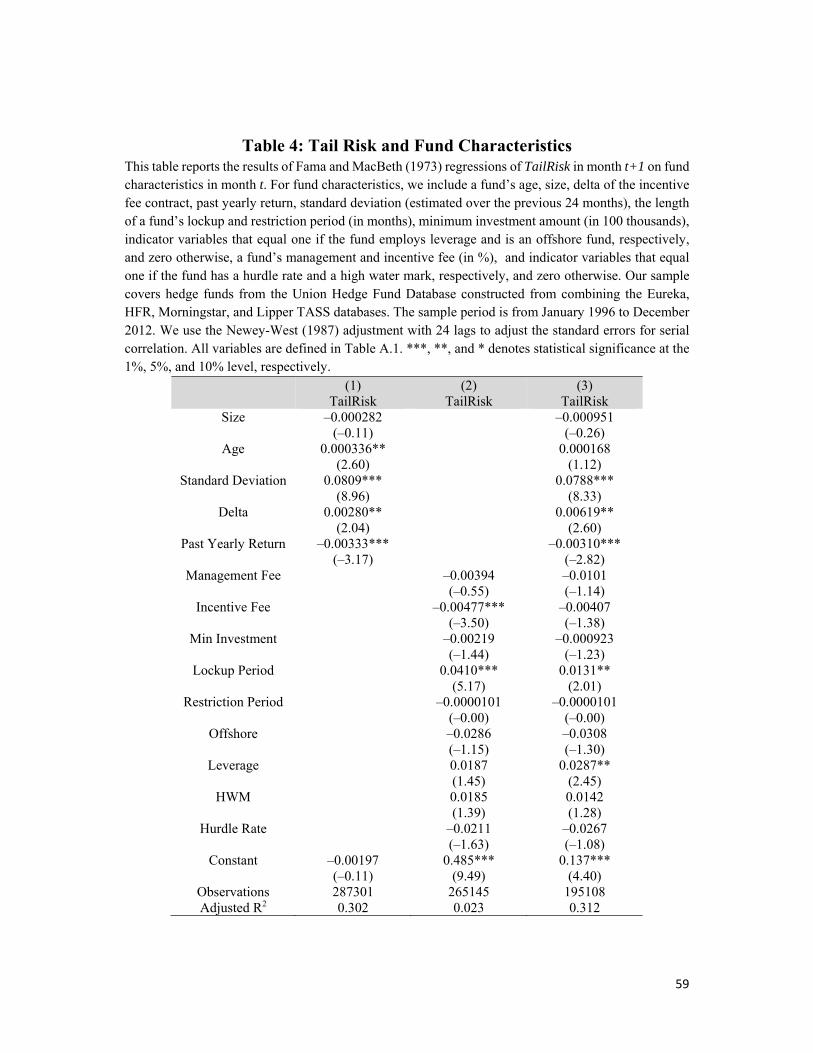
59  

Table 4: Tail Risk and Fund Characteristics This table reports the results of Fama and MacBeth (1973) regressions of TailRisk in month t+1 on fund characteristics in month t. For fund characteristics, we include a fund’s age, size, delta of the incentive fee contract, past yearly return, standard deviation (estimated over the previous 24 months), the length of a fund’s lockup and restriction period (in months), minimum investment amount (in 100 thousands), indicator variables that equal one if the fund employs leverage and is an offshore fund, respectively, and zero otherwise, a fund’s management and incentive fee (in %), and indicator variables that equal one if the fund has a hurdle rate and a high water mark, respectively, and zero otherwise. Our sample covers hedge funds from the Union Hedge Fund Database constructed from combining the Eureka, HFR, Morningstar, and Lipper TASS databases. The sample period is from January 1996 to December 2012. We use the Newey-West (1987) adjustment with 24 lags to adjust the standard errors for serial correlation. All variables are defined in Table A.1. ***, **, and * denotes statistical significance at the 1%, 5%, and 10% level, respectively.

(1) TailRisk

(2) TailRisk

(3) TailRisk

Size ‒0.000282 (‒0.11)

‒0.000951 (‒0.26)

Age 0.000336** (2.60)

0.000168 (1.12)

Standard Deviation 0.0809*** (8.96)

0.0788*** (8.33)

Delta 0.00280** (2.04)

0.00619** (2.60)

Past Yearly Return ‒0.00333*** (‒3.17)

‒0.00310*** (‒2.82)

Management Fee ‒0.00394 (‒0.55)

‒0.0101 (‒1.14)

Incentive Fee ‒0.00477*** (‒3.50)

‒0.00407 (‒1.38)

Min Investment ‒0.00219 (‒1.44)

‒0.000923 (‒1.23)

Lockup Period 0.0410*** (5.17)

0.0131** (2.01)

Restriction Period ‒0.0000101 (‒0.00)

‒0.0000101 (‒0.00)

Offshore ‒0.0286 (‒1.15)

‒0.0308 (‒1.30)

Leverage 0.0187 (1.45)

0.0287** (2.45)

HWM 0.0185 (1.39)

0.0142 (1.28)

Hurdle Rate ‒0.0211 (‒1.63)

‒0.0267 (‒1.08)

Constant ‒0.00197 (‒0.11)

0.485*** (9.49)

0.137*** (4.40)

Observations 287301 265145 195108 Adjusted R2 0.302 0.023 0.312

60  

Table 5: Tail Risk and Funding Liquidity: Evidence from Lehman Brothers connected Hedge Funds

Panel A of this table reports the results of a mean comparison test between the TailRisk for equity-related hedge funds with Lehman Brothers as a prime broker and TailRisk for a matched sample (matched both on propensity scores as well as based on the requirement that matched funds belong to the same hedge fund style category as well as the same TailRisk, size, and monthly excess returns decile in August 2007) in the periods from September 2007 to August 2008 (Pre-Crisis), September 2008 to August 2009 (Crisis), and September 2009 to August 2010 (Post-Crisis). Panel B present the results from the following diff-in-diff regression:

, 1 2 3 , 1 ,i t Postcrisis Crisis Crisis-Precrisis Postcrisis Crisis i t i tTailRisk Lehman Lehman X

where ,i tTailRisk denotes the change in tail risk for hedge fund i between the pre-Lehman crisis and the crisis period, or between the crisis and the post-crisis

period, respectively. Crisis-Precrisis and Postcrisis Crisis are indicator variables for the period between Crisis and Pre-Crisis, and Post-Crisis and Crisis, respectively,

where the respective periods are defined as in Panel A. Lehman is an indicator variable that takes on the value one if a fund has a prime brokerage relation with Lehman Brothers, and zero otherwise. , 1i tX is a vector of fund-specific control variables that includes age, size, delta, returns over the last one year, standard

deviation estimated over the previous year, lockup period, restriction period, minimum investment, management fee, incentive fee, and indicator variables whether the fund employs leverage, is an offshore fund, uses a hurdle rate, and uses a high water mark, all measured at time t‒1. We estimate TailRisk based on an estimation period of 12 months and cluster standard errors by fund. All variables are defined in Table A.1. ***, **, and * denotes statistical significance at the 1%, 5%, and 10% level, respectively.

Panel A: TailRisk: Mean Comparison Tests Period 1: September 2007 - August 2008 Period 2: September 2008 - August 2009 Period 3: September 2009 - August 2010 Lehman

Hedge Funds Matched Sample Non-connected

Difference Lehman

Hedge Funds Matched Sample Non-connected

Difference Lehman

Hedge Funds Matched Sample Non-connected

Difference

Match: Propensity Score Model

0.39 0.45 ‒0.06

(‒0.56)0.82 0.57

0.25** (2.01)

0.13 0.16 ‒0.03

(‒0.48)Match: Style, TailRisk, Size, and Returns in August 2007

0.39 0.44 ‒0.05

(‒0.39) 0.82 0.55

0.27** (2.25)

0.13 0.15 ‒0.02

(‒0.39)

61  

Table 5: (Continued)

Panel B: Diff-in-Diff Analysis

Match: Propensity Score Model

Match: Style, TailRisk, Size, and Returns

(1) TailRisk Change

(2) TailRisk Change

(3) TailRisk Change

(4) TailRisk Change

Postcrisis Crisis ‒0.553*** (‒5.71)

‒0.516*** (‒4.11)

‒0.575*** (‒6.10)

‒0.586*** (‒5.78)

Crisis-Precrisis Lehman 0.321** (2.20)

0.272* (1.85)

0.351** (2.26)

0.252* (1.90)

Postcrisis Crisis Lehman ‒0.253** (‒2.02)

‒0.228* (‒1.81)

‒0.281** (‒2.22)

‒0.221* (‒1.85)

Age ‒0.003 (‒1.15)

‒0.000 (‒0.11)

Size 0.006 (1.04)

0.013 (1.21)

Delta ‒0.211 (‒1.31)

‒0.149 (‒1.21)

Past Yearly Return ‒0.034 (‒1.13)

‒0.091** (‒2.13)

Standard Deviation 0.076 (0.32)

‒0.036 (‒0.05)

Lockup Period ‒0.0004 (‒0.02)

‒0.0024 (‒0.71)

Restriction Period ‒0.048 (‒0.34)

‒0.093 (‒0.93)

Min Investment 0.023 (0.89)

0.099* (1.89)

Leverage 0.077** (2.15)

0.078** (2.00)

Offshore ‒0.021 (‒0.56)

0.052 (1.46)

Management Fee 0.003 (0.14)

0.007 (0.64)

Incentive Fee 0.008 (1.12)

0.034* (1.88)

Hurdle Rate 0.098 (1.24)

0.018 (0.83)

HWM ‒0.099 (‒1.56)

‒0.059 (‒0.96)

Constant 0.210***

(8.45) 0.415***

(3.26) 0.214***

(7.75) 0.447***

(3.51)

Observations 2627 2049 2627 2049 Adjusted R2 0.180 0.312 0.180 0.312

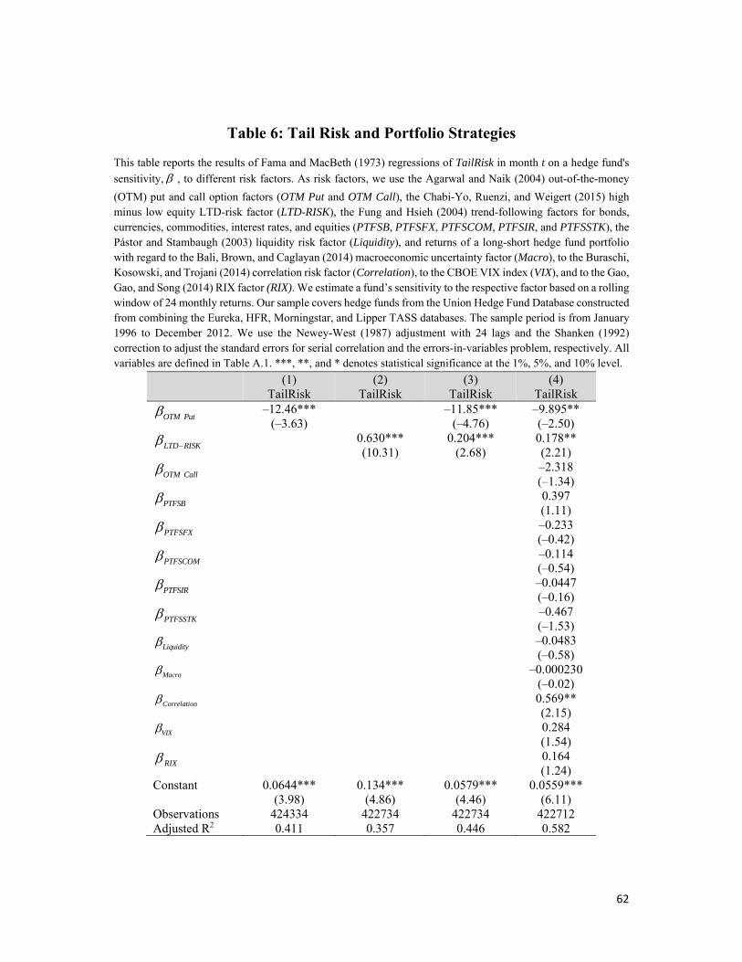
62  

Table 6: Tail Risk and Portfolio Strategies

This table reports the results of Fama and MacBeth (1973) regressions of TailRisk in month t on a hedge fund's

sensitivity, , to different risk factors. As risk factors, we use the Agarwal and Naik (2004) out-of-the-money

(OTM) put and call option factors (OTM Put and OTM Call), the Chabi-Yo, Ruenzi, and Weigert (2015) high minus low equity LTD-risk factor (LTD-RISK), the Fung and Hsieh (2004) trend-following factors for bonds, currencies, commodities, interest rates, and equities (PTFSB, PTFSFX, PTFSCOM, PTFSIR, and PTFSSTK), the Pástor and Stambaugh (2003) liquidity risk factor (Liquidity), and returns of a long-short hedge fund portfolio with regard to the Bali, Brown, and Caglayan (2014) macroeconomic uncertainty factor (Macro), to the Buraschi, Kosowski, and Trojani (2014) correlation risk factor (Correlation), to the CBOE VIX index (VIX), and to the Gao, Gao, and Song (2014) RIX factor (RIX). We estimate a fund’s sensitivity to the respective factor based on a rolling window of 24 monthly returns. Our sample covers hedge funds from the Union Hedge Fund Database constructed from combining the Eureka, HFR, Morningstar, and Lipper TASS databases. The sample period is from January 1996 to December 2012. We use the Newey-West (1987) adjustment with 24 lags and the Shanken (1992) correction to adjust the standard errors for serial correlation and the errors-in-variables problem, respectively. All variables are defined in Table A.1. ***, **, and * denotes statistical significance at the 1%, 5%, and 10% level.

(1) TailRisk

(2) TailRisk

(3) TailRisk

(4) TailRisk

OTM Put ‒12.46*** (‒3.63)

‒11.85*** (‒4.76)

‒9.895** (‒2.50)

LTD RISK 0.630*** (10.31)

0.204*** (2.68)

0.178** (2.21)

OTM Call ‒2.318 (‒1.34)

PTFSB 0.397 (1.11)

PTFSFX ‒0.233 (‒0.42)

PTFSCOM ‒0.114 (‒0.54)

PTFSIR ‒0.0447 (‒0.16)

PTFSSTK ‒0.467 (‒1.53)

Liquidity ‒0.0483 (‒0.58)

Macro ‒0.000230 (‒0.02)

Correlation 0.569** (2.15)

VIX 0.284 (1.54)

RIX 0.164 (1.24)

Constant 0.0644*** (3.98)

0.134*** (4.86)

0.0579*** (4.46)

0.0559*** (6.11)

Observations 424334 422734 422734 422712 Adjusted R2 0.411 0.357 0.446 0.582

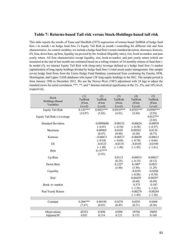
63  

Table 7: Returns-based Tail risk versus Stock-Holdings-based tail risk

This table reports the results of Fama and MacBeth (1973) regressions of returns-based TailRisk of hedge fund firm i in month t on hedge fund firm i’s Equity Tail Risk in month t controlling for different risk and firm characteristics. As control variables, we include a hedge fund firm’s return standard deviation, skewness, kurtosis, ES, beta, down beta, up beta, liquidity (as proxied by the Amihud illiquidity ratio), size, book-to-market, and past yearly return. All firm characteristics except liquidity, size, book-to-market, and past yearly return (which are measured at the end of last month) are estimated based on a rolling window of 24 monthly returns of fund firm i. In model (5), we interact Equity Tail Risk with (long-only) leverage defined as a hedge fund firm i’s market capitalization of long equity holdings divided by hedge fund firm i’s total assets under management. Our sample covers hedge fund firms from the Union Hedge Fund Database constructed from combining the Eureka, HFR, Morningstar, and Lipper TASS databases who report 13F long equity holdings to the SEC. The sample period is from January 1996 to December 2012. We use the Newey-West (1987) adjustment with 24 lags to adjust the standard errors for serial correlation. ***, **, and * denotes statistical significance at the 1%, 5%, and 10% level, respectively.

Stock Holdings-Based

Variables

(1) TailRisk (Firm Level)

(2) TailRisk

(Firm Level)

(3) TailRisk

(Firm Level)

(4) TailRisk

(Firm Level)

(5) TailRisk

(Firm Level)

Equity Tail Risk 0.145*** (14.97)

0.0923*** (5.03)

0.0918*** (4.91)

0.0793*** (3.69)

0.0590*** (2.93)

Equity Tail Risk x Leverage 0.0127** (2.02)

Standard Deviation ‒0.0000680 (‒0.01)

‒0.00133 (‒0.10)

‒0.00624 (‒0.38)

‒0.00939 (‒0.57)

Skewness 0.00969 (0.47)

0.0105 (0.48)

0.00563 (0.28)

0.0136 (0.73)

Kurtosis ‒0.00411 (‒0.54)

‒0.00517 (‒0.69)

‒0.00699 (‒0.78)

‒0.00613 (‒0.66)

ES ‒0.0123 (‒1.48)

‒0.0135 (‒1.48)

‒0.0169 (‒1.45)

‒0.0190 (‒1.61)

Beta 0.157*** (3.02)

Up Beta 0.0113 (0.25)

‒0.00915 (‒0.15)

0.00637 (0.12)

Down Beta 0.122* (1.86)

0.108* (1.94)

0.0821 (1.29)

Liquidity ‒0.0391 (‒0.88)

‒0.0288 (‒0.70)

Size 0.00439 (0.64)

0.00297 (0.49)

Book‒to‒market ‒0.373 (‒1.56)

‒0.347 (‒1.62)

Past Yearly Return ‒0.00279 (‒1.42)

‒0.00264 (‒1.36)

Constant 0.206***

(7.67) 0.00190 (0.03)

0.0270 (0.45)

0.0293 (0.31)

0.0468 (0.56)

Observations 42353 41896 41896 39708 39695 Adjusted R2 0.051 0.114 0.121 0.153 0.169

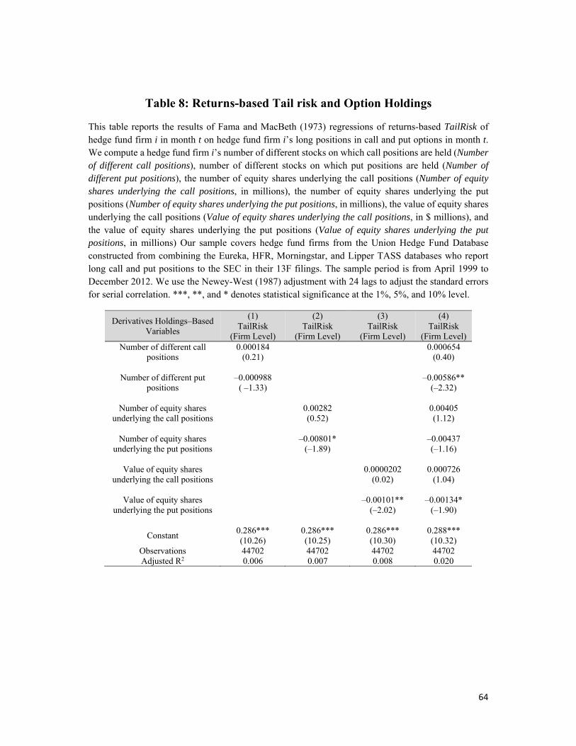
64  

Table 8: Returns-based Tail risk and Option Holdings

This table reports the results of Fama and MacBeth (1973) regressions of returns-based TailRisk of hedge fund firm i in month t on hedge fund firm i’s long positions in call and put options in month t. We compute a hedge fund firm i’s number of different stocks on which call positions are held (Number of different call positions), number of different stocks on which put positions are held (Number of different put positions), the number of equity shares underlying the call positions (Number of equity shares underlying the call positions, in millions), the number of equity shares underlying the put positions (Number of equity shares underlying the put positions, in millions), the value of equity shares underlying the call positions (Value of equity shares underlying the call positions, in $ millions), and the value of equity shares underlying the put positions (Value of equity shares underlying the put positions, in millions) Our sample covers hedge fund firms from the Union Hedge Fund Database constructed from combining the Eureka, HFR, Morningstar, and Lipper TASS databases who report long call and put positions to the SEC in their 13F filings. The sample period is from April 1999 to December 2012. We use the Newey-West (1987) adjustment with 24 lags to adjust the standard errors for serial correlation. ***, **, and * denotes statistical significance at the 1%, 5%, and 10% level.

Derivatives Holdings‒Based Variables 

(1) TailRisk

(Firm Level)

(2) TailRisk

(Firm Level)

(3) TailRisk

(Firm Level)

(4) TailRisk

(Firm Level) Number of different call

positions 0.000184

(0.21)

0.000654 (0.40)

Number of different put

positions ‒0.000988

( ‒1.33)

‒0.00586** (‒2.32)

Number of equity shares

underlying the call positions

0.00282 (0.52)

0.00405 (1.12)

Number of equity shares

underlying the put positions

‒0.00801* (‒1.89)

‒0.00437 (‒1.16)

Value of equity shares

underlying the call positions

0.0000202 (0.02)

0.000726 (1.04)

Value of equity shares

underlying the put positions

‒0.00101** (‒2.02)

‒0.00134* (‒1.90)

Constant 0.286*** (10.26)

0.286*** (10.25)

0.286*** (10.30)

0.288*** (10.32)

Observations 44702 44702 44702 44702 Adjusted R2 0.006 0.007 0.008 0.020

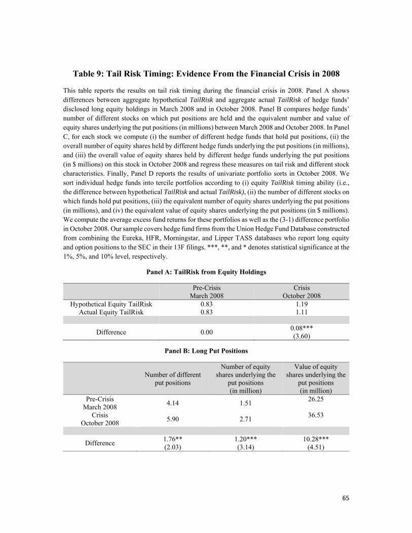
65  

Table 9: Tail Risk Timing: Evidence From the Financial Crisis in 2008

This table reports the results on tail risk timing during the financial crisis in 2008. Panel A shows differences between aggregate hypothetical TailRisk and aggregate actual TailRisk of hedge funds’ disclosed long equity holdings in March 2008 and in October 2008. Panel B compares hedge funds’ number of different stocks on which put positions are held and the equivalent number and value of equity shares underlying the put positions (in millions) between March 2008 and October 2008. In Panel C, for each stock we compute (i) the number of different hedge funds that hold put positions, (ii) the overall number of equity shares held by different hedge funds underlying the put positions (in millions), and (iii) the overall value of equity shares held by different hedge funds underlying the put positions (in $ millions) on this stock in October 2008 and regress these measures on tail risk and different stock characteristics. Finally, Panel D reports the results of univariate portfolio sorts in October 2008. We sort individual hedge funds into tercile portfolios according to (i) equity TailRisk timing ability (i.e., the difference between hypothetical TailRisk and actual TailRisk), (ii) the number of different stocks on which funds hold put positions, (iii) the equivalent number of equity shares underlying the put positions (in millions), and (iv) the equivalent value of equity shares underlying the put positions (in $ millions). We compute the average excess fund returns for these portfolios as well as the (3-1) difference portfolio in October 2008. Our sample covers hedge fund firms from the Union Hedge Fund Database constructed from combining the Eureka, HFR, Morningstar, and Lipper TASS databases who report long equity and option positions to the SEC in their 13F filings. ***, **, and * denotes statistical significance at the 1%, 5%, and 10% level, respectively.

Panel A: TailRisk from Equity Holdings

Pre-Crisis

March 2008Crisis

October 2008 Hypothetical Equity TailRisk 0.83 1.19

Actual Equity TailRisk 0.83 1.11

Difference 0.00 0.08*** (3.60)

Panel B: Long Put Positions

Number of different

put positions

Number of equity shares underlying the

put positions (in million)

Value of equity shares underlying the

put positions (in million)

Pre-Crisis March 2008

4.14 1.51 26.25

Crisis October 2008

5.90 2.71 36.53

Difference 1.76** (2.03)

1.20*** (3.14)

10.28*** (4.51)

66  

Table 9: (Continued) Panel C: Put Options and Stock Characteristics

Stock Holdings-Based

Variables

(1) Number of Hedge

Funds with Puts

(2) Number of

Equity Shares Held by Hedge

Funds

(3) Value of Equity

Shares Held by Hedge

Funds

(4) Number of

Hedge Funds with

Puts

(5) Number of

Equity Shares

Held by Hedge Funds

(6) Value of Equity

Shares Held by Hedge

Funds

Equity Tail Risk 1.726*** (7.21)

0.537** (2.11)

10.33** (2.34)

0.709*** (3.37)

0.112 (0.38)

5.535* (1.83)

Standard Deviation 0.541*** (13.09)

0.428*** (7.71)

7.462*** (8.45)

Skewness 0.237*** (5.30)

0.307*** (5.40)

5.819*** (5.96)

Kurtosis 0.00769** (2.05)

0.0128* (1.68)

0.0682 (0.85)

Beta ‒0.0616 (‒0.51)

‒0.280 (‒1.64)

‒11.80*** (‒4.07)

Liquidity 0.0769*** (15.26)

0.0600*** (8.42)

1.290*** (9.70)

Size 1.393*** (26.65)

0.970*** (10.95)

20.60*** (11.64)

Book‒to‒market 0.0752* (1.92)

0.114* (1.70)

2.643*** (2.82)

Past Yearly Return ‒2.768*** (‒13.01)

‒2.143*** (‒8.28)

‒37.66*** (‒8.82)

Constant 1.114***

(12.48) 0.580***

(5.92) 9.764***

(5.77) ‒17.25*** (‒24.32)

‒12.33*** (‒10.37)

‒257.9*** (‒11.22)

Observations 4211 4211 4211 3801 3801 3801 Adjusted R2 0.019 0.002 0.002 0.472 0.204 0.239

Panel D: Fund Firm Performance Differences in October 2008

Equity TailRisk Timing

Number of different put

positions

Number of equity shares underlying the put positions

(in million)

Value of equity shares underlying the put positions

(in million) PF 1 ‒9.57% ‒10.06% ‒9.11% ‒8.88% PF 2 ‒8.14% ‒6.96% ‒7.50% ‒6.90% PF 3 ‒5.34% ‒5.00% ‒5.05% ‒5.27%

PF3 ‒ PF1 4.23%***

(2.95) 5.06%***

(3.69) 4.06%***

(3.01) 3.61%* (1.82)