TAG UNIT A2.1

Wider Impacts

January 2014

Department for Transport

Transport Analysis Guidance (TAG)

https://www.gov.uk/transport-analysis-guidance-webtag

This TAG Unit is guidance for the APPRAISAL PRACTITIONER This TAG Unit is part of the family A2 – ECONOMIC IMPACTS Technical queries and comments on this TAG Unit should be referred to: Transport Appraisal and Strategic Modelling (TASM) Division Department for Transport Zone 2/25 Great Minster House 33 Horseferry Road London SW1P 4DR tasm@dft.gsi.gov.uk

This file has been updated. For the most up-to-date version of this unit please refer to the WebTAG website.

Contents

1 Overview 1

1.1 Introduction 1

2 Development and application of methods for assessment of Wider Impacts 1

2.2 Types of Wider Impacts 2

3 Scope of the Wider Impacts Assessment 3

4 Calculation of Wider Impacts Estimates 3

4.1 Calculating the Scheme Impacts 3 4.2 Profiling over the Appraisal Period 7 4.3 Application of Sensitivity Tests 7

5 Data Used in Wider Impacts Assessment 8

5.1 Collation of Data 8 5.2 Identifying and Resolving Problems with Data 10

6 Application of the Wider Impacts Analysis Checklist 13

7 Reporting Results from the Wider Impacts Assessment 15

8 References 18

9 Document Provenance 18

Appendix A Functional Urban Regions (FURs) 19

Appendix B Data summary 21

Appendix C Sectoral Aggregation Information from UK SIC(92) 2 digit Classification 25

Appendix D Equations for Calculation of Wider Impacts 26

TAG Unit A2.1 Wider Impacts

Page 2

Impacts, the reasons for this decision should be reported in the Appraisal Specification Report

(ASR).

2.1.3 Alongside this guidance, software has been developed, Wider Impacts in Transport Appraisal

(WITA) that can be used for estimation of Wider Impacts. However, use of this software is not

essential and other software or workbooks can also be developed and applied for estimation of

Wider Impacts. It is required that these should generate the Wider Impacts estimates in a way that is

consistent with the guidance in this Unit, and should be able to show clearly how the estimates were

generated, so that estimates can be independently checked and verified.

2.2 Types of Wider Impacts

WI1 - Agglomeration Impacts

2.2.1 The term “agglomeration” refers to the concentration of economic activity over an area. Transport

can alter the accessibility of firms in an area to other firms and workers, thereby affecting the level of

agglomeration.

2.2.2 Agglomeration impacts arise because firms derive productivity benefits from being close to one

another and from being located in large labour markets. If transport investment brings firms closer

together and closer to their workforce this may generate an increase in labour productivity above

and beyond that which would be expected from the direct user benefits alone.

2.2.3 Greater productivity in agglomerations arises from the fact that firms have access to larger product,

input and labour markets. Knowledge and technology spillovers are also important aspects of

agglomeration effects.

WI2 - Output Change in Imperfectly Competitive Markets

2.2.4 A reduction in transport costs (to business and/or freight) allows firms to profitably increase output of

the goods or services that require use of transport in their production.

2.2.5 A transport intervention that leads to increased output of goods and services will deliver a welfare

gain as consumers’ willingness to pay for the increased output will exceed the cost of producing it.

WI3 - Tax revenues arising from labour market impacts (including labour supply impacts and

moves to more or less productive jobs)

2.2.6 Changes in transport provision and costs can affect labour market decisions. Two main types of

labour market impacts have been identified. These are referred to as “labour supply” impacts, and

“moves to more or less productive jobs” impacts

2.2.7 Transport costs are likely to affect the overall costs and benefits to an individual from working. In

deciding whether or not to work, an individual will weigh the costs associated with work, including

travel costs, against the wage rate of the job travelled to. A change in transport costs alters the net

financial return to individuals from employment. This is likely to affect the incentives of individuals to

work, and therefore the numbers choosing to work and the overall amount of labour supplied in the

economy.

2.2.8 Transport can also affect the decisions made by firms and workers about where to locate and work.

Employment growth or decline in different areas is likely to have implications for productivity, as

workers are often more or less productive in different locations.

2.2.9 Some of the economic effects of these impacts are captured in commuter user benefits. However,

commuter user benefits do not include the change in tax revenues received by the government.

Changes in tax revenues are excluded from commuter user benefits because commuters value

benefits in terms of post tax incomes.

TAG Unit A2.1 Wider Impacts

Page 5

4.1.10 These impacts are calculated from the business user benefits in the Transport Economic Efficiency

(TEE) analysis. The impact would be positive where business user benefits are positive overall, and

negative where business user benefits associated with the transport scheme are negative7

WI3 - Tax Revenue from Labour Market Impacts

4.1.11 The welfare benefits from labour market impacts are partially captured in commuter user benefits

but the tax implications are not and to estimate them it is necessary to quantify the full effects of

labour supply impacts, and move to more or less productive jobs impacts, and then apply the

relevant rate of taxation

Labour Supply Impact

4.1.12 Transport costs are likely to affect the overall costs and benefits to an individual from working. In

deciding whether to work, an individual will weigh the costs of working, including travel costs,

against the wage rate of the job travelled to.

4.1.13 The calculation of the labour supply impact estimates the additional value that is generated if a

transport improvements changes travel costs, and therefore affects the number of people attracted

into work. The calculation is done in three parts:

i) calculating how commuting costs for round trips change as a result of the scheme and how this

will affect the benefit an individual obtains from working;

ii) calculating how the change in the benefit from working will impact on the overall amount of

labour supplied; and

iii) calculating the additional national output produced by the new labour supplied.

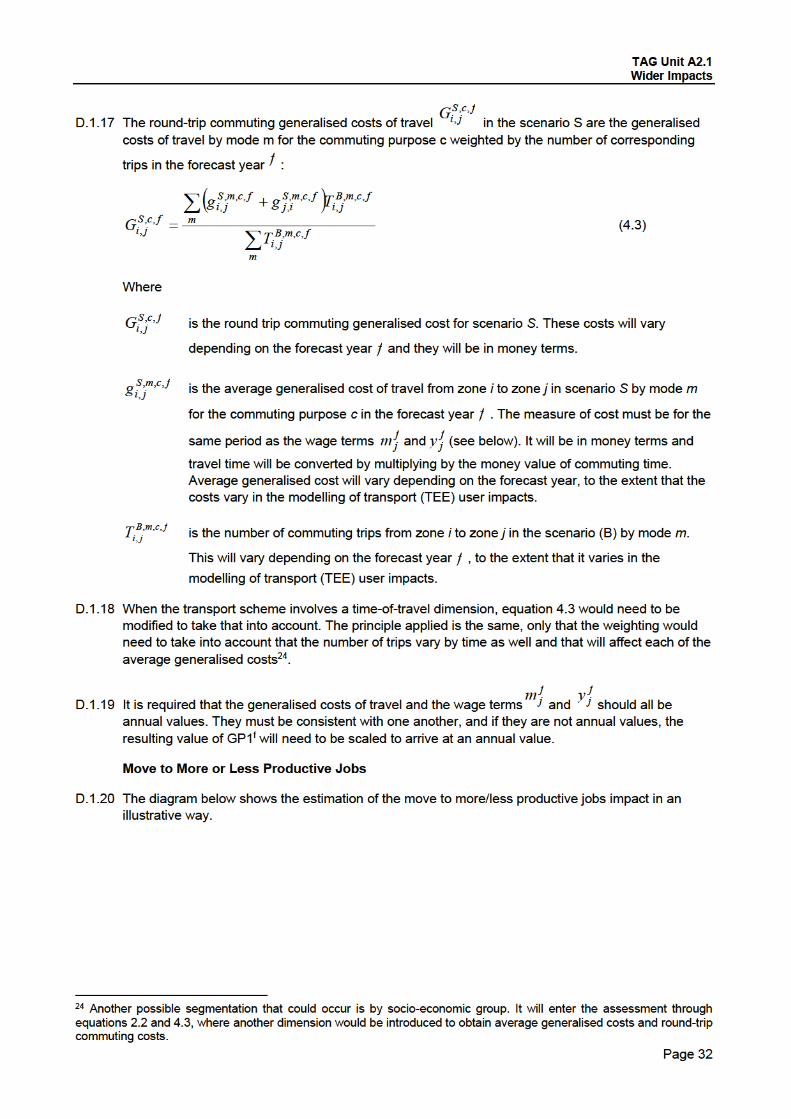
4.1.14 The first step is to estimate the average generalised cost for workers commuting from each origin

(home) zone to each destination (employment) zone, and from this to find the average change in

commuting generalised costs for each worker from the Base to the Alternative case.

4.1.15 The output of this step is a set of estimated changes in annual costs of commuting per worker by

zone pair and year. This change in annual commuting costs can be considered as a change in the

perceived annual return from working. It is divided by the earnings of the workers working in the

destination zone to give the perceived relative change in net earnings. It is assumed that all savings

are passed on to workers.

4.1.16 In the second step, the labour supply elasticity with respect to wages in absolute value is used

to convert the perceived relative change in net earnings to a relative change in labour supply by

zone pair.

4.1.17 The relative change in labour participation is weighted by the number of workers living in the origin

zone and working in the destination zone and then multiplied by the median8 wage of the marginal

worker outside of employment (who is assumed to be less productive than the average worker) in

employment in the destination zone.

4.1.18 This process is repeated and added for all origin (home) zones. The final output of this section is the

total productivity change from the increased or decreased labour supply, for each year9.

7 It is more likely that the transport scheme will result in an increase in output, as the transport scheme would try to provide an optimal level of transport provision that drives marginal costs down. However, in some cases where schemes increase travel costs, the marginal cost of transport could go up as a result of the intervention. 8 Using median rather than average wage has the advantage of eliminating the potential small number of outliers with very high wages that would otherwise skew the average wage. 9 The additional profit for firms as a result of taking on the extra workers, (the tax take on marginal profit), is already included in the TEE appraisal.

TAG Unit A2.1 Wider Impacts

Page 6

4.1.19 Changes in residential location may also affect the level of labour participation. Where a transport

scheme affects the residential location of those not participating in the labour market there is the

potential for the transport scheme to result in a change in labour participation, through its impact on

average generalised cost of travel to jobs. Where residential relocation is modelled and fed into the

estimated labour supply impact, the results must be reported as sensitivity estimates and not in the

central case. Central case estimates must assume that residential location is fixed.

Move to More or Less Productive Jobs

4.1.20 Changes in transport costs are likely to affect the overall costs and benefits to an individual from

working in different locations and the benefits to business of operating and employing people in

different locations. This can potentially result in jobs moving between locations with differential

productivity levels.

4.1.21 Changes in the location of employment are likely to impact on the overall productivity of

employment. The estimation of the ‘move to more productive jobs’ impact consists of two stages.

The first stage is modelling the impact of the transport scheme on the location of employment. The

second stage is estimating the impact of the changes in employment location on productivity.

4.1.22 The impact on the location of employment should be calculated only when a Land Use Transport

Interaction (LUTI) model is used to forecast the employment and residential location consequences

of the scheme that is being appraised

4.1.23 An index of productivity differentials for Local Authority Districts (LADs) is provided in the Wider

Impacts Dataset. This index is used to estimate the productivity impacts from the modelled

relocation of employment. For each Local Authority District, the ‘Move to More/Less Productive

Jobs’ impact is estimated by multiplying the change in employment in the area, resulting from the

transport intervention, by the indexed ‘GDP per worker’ in the area and then summing across areas.

The output of this step is the change in total output from the ‘Move to More/Less Productive Jobs’

effect, for each year.

4.1.24 A LUTI model can also be used to estimate changes in residential location that form part of the

modelled response to the transport scheme. These changes in residential location will feed into the

estimates of commuter user impacts, and could therefore be expected to affect the level of

employment in different zones in the Alternative case.

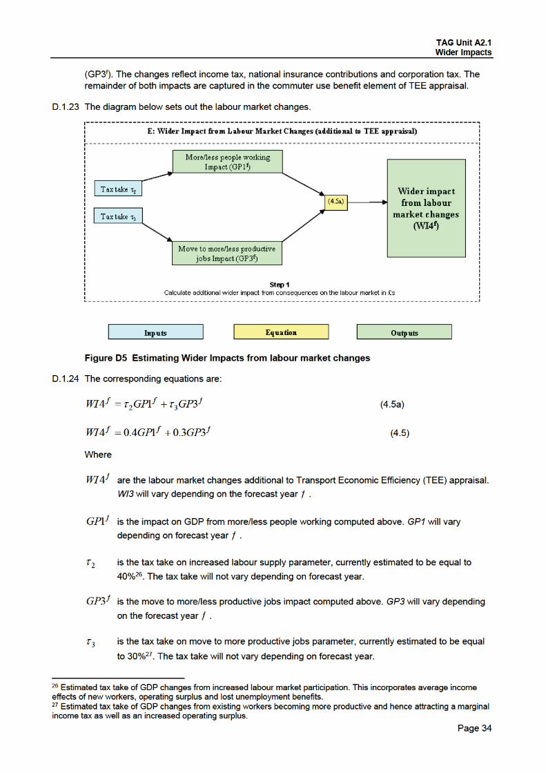
Tax Revenues Arising from Labour Market Impacts

4.1.25 The change in tax revenues that results from the labour market impacts is estimated from the

change in GDP from the labour supply impact, and from the move to more or less productive jobs

impacts. It is estimated to be 40% of the change in GDP from the labour supply impact, and 30% of

the change in GDP from the move to more or less productive jobs impact.

Impact of Transport of Employment Location and Residential Location

4.1.26 The ‘central case’ Wider Impacts estimate should assume no change in employment or residential

location from the Base case. The estimation of the impact of transport on employment location

across areas and over time is challenging and generally requires a Land Use Transport Interaction

(LUTI) model. However, if a suitable model is used, ‘sensitivity estimates’ can be produced for the

move to more or less productive jobs, labour supply impacts, and agglomeration.

4.1.27 The central case assumes no change in employment/residential location. These may be assessed

in a sensitivity case if a LUTI model is available.

4.1.28 In some instances, a transport scheme may be expected to have an impact on employment location

and residential location that should at least be noted if not analysed in detail. In these situations, the

type of analysis applied should be clearly identified.

https://www.gov.uk/transport-analysis-guidance-webtag#a1-cost-benefit-analysis

TAG Unit A2.1 Wider Impacts

Page 9

Agglomeration

Table 1 Agglomeration Data

Data Value

Local GDP per Worker by Local Authority District

Sectoral Employment Forecasts by Local Authority District

Total Employment Forecasts by Local Authority District

Agglomeration Elasticities by

industrial sector

manufacturing = 0.021

construction = 0.034

consumer services = 0.024

producer services = 0.083

Parameter for exponential decay of

effective density with generalised

costs for different sectors

manufacturing = 1.097

construction = 1.562

consumer services = 1.818

producer services = 1.746

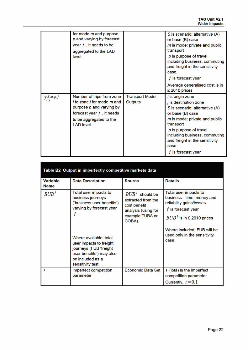
Output in imperfectly competitive markets

5.1.4 The value of the parameter for imperfect competition is 0.1.

Tax Revenue from Labour Market Impacts

Table 2 Data for Tax Revenue from Labour Market Impacts

Data Value

Elasticity of labour supply with respect to net return

from working

0.1

Average workplace-based earnings by Local Authority District

Productivity parameter that captures the lower

productivity of new entrants to the labour force (pay

of marginal worker compared to average worker)

0.69

Average National GDP per worker by forecast year

Index of Productivity per Worker by Local Authority District

Average tax rate on earnings 0.3

Parameter for Tax take on Labour Supply 0.4

Parameter for Tax take on Move to More/Less

Productive Jobs

0.3

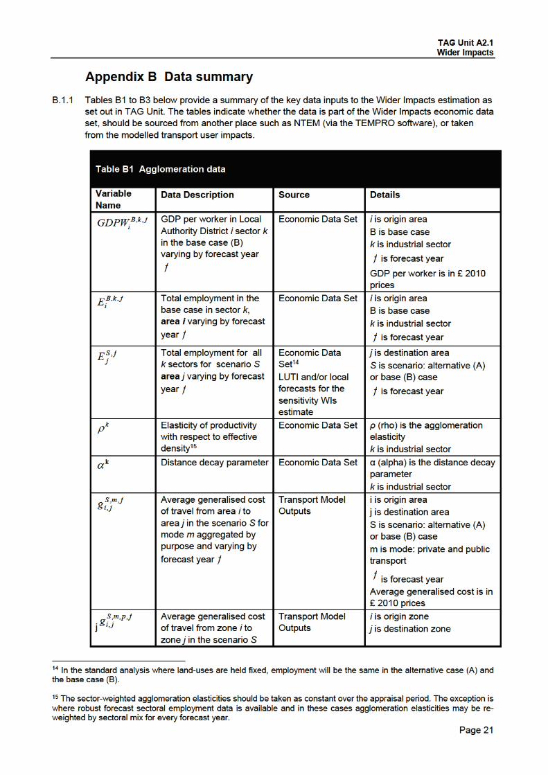
5.1.5 Appendix B provides a detailed summary of each of these key data inputs required for the

calculation of Wider Impacts.

Transport Model Data: Overview

5.1.6 The estimation of Wider Impacts builds on the modelled user benefits. If transport model data for all

relevant modes11 are not incorporated into the assessment, then this is likely to result in errors in the

estimation of Wider Impacts. This is because the omission of relevant modes will lead to an

incorrect estimation of the Base case level of agglomeration and hence an incorrect estimation of

the productivity impact resulting from any changes in agglomeration caused by the transport

scheme.

11 For the purpose of Wider Impacts analysis, ‘relevant modes’ refers to all modes that are utilised in the modelled area in the base case as well as all modes that are affected by the intervention itself.

TAG Unit A2.1 Wider Impacts

Page 10

5.1.7 Similarly geographic coverage is important. The study area should be limited to the area in which

the modelling provides a good estimate of Base generalised costs. Data on demand and

generalised cost are required for all flows, whether they are affected by the modelled intervention or

not.

5.1.8 The need for a good estimate of Base generalised costs may be a particular issue for rail where

multi-modal models are not usually available in scheme appraisals. Further information on

considering adequate mode coverage is provided in section 5 of this Unit.

Transport Model Data: Demand

5.1.9 Demand data should be extracted from the transport model for the full set of Origin and Destination

(OD) pairs and segmented by mode, journey purpose and across time periods. The OD matrices

extracted then need to be aggregated to match the level of aggregation for the economic data,

normally to Local Authority District (LAD) level.

Transport Model Data: Generalised Cost

5.1.10 Generalised cost data should also be extracted from the transport model for the full set of OD pairs,

and including all users and modes.

5.1.11 The Wider Impacts assessment analyses the change in accessibility for different transport users and

the benefits that derive as a result of this change in accessibility beyond direct user benefits. To

allow for this, the measure of the generalised cost change (resulting from the scheme) needs to be

as full a measure as possible. This means it needs to capture time, travel cost, reliability and

crowding benefits, where relevant.

5.1.12 The costs used should be calculated in 2010 prices and as a weighted average across user groups,

aggregated according to shares of different user groups (e.g. Commuting and Business/In-Work).

Geographical Detail of Data

5.1.13 The economic and transport data are often sourced at different levels of geographic detail. The

Wider Impact methodology largely uses data generated from transport modelling, building on

modelled inputs to the TUBA cost benefit analysis. Specific inputs to the Wider Impacts assessment

of accessibility change include estimates of user demand for the different journey purposes and

modes in the Base case and Alternative case scenarios. The main source for such data is model

O/D matrices of travel flows used in TUBA.

5.1.14 The inputs also include estimates of changes in generalised travel cost for each of the user groups

and modes, for the different modelled years. Again, the main source for such data is the modelled

input generalised cost information for TUBA.

5.1.15 The economic data set is put together at Local Authority District (LAD) level. The modelled transport

demand and generalised cost data is likely to be at the level of geography selected for the transport

zones of the transport model. This will vary in different cases, and will often be at a lower, more

detailed level of geography than the economic data. In these cases the transport data will need to

be aggregated to LAD level to put the transport and economic data on the same level of geographic

detail for analysis.

5.2 Identifying and Resolving Problems with Data

Overview

5.2.1 The calculation of Wider Impacts involves greater data demands than is required for estimation of

user benefits. In a standard analysis of user benefits, only demand levels and changes in

generalised costs are required. Journeys for which generalised costs and demand do not change

are irrelevant to the calculations. In contrast, agglomeration estimates require accessibility

TAG Unit A2.1 Wider Impacts

Page 13

6 Application of the Wider Impacts Analysis Checklist

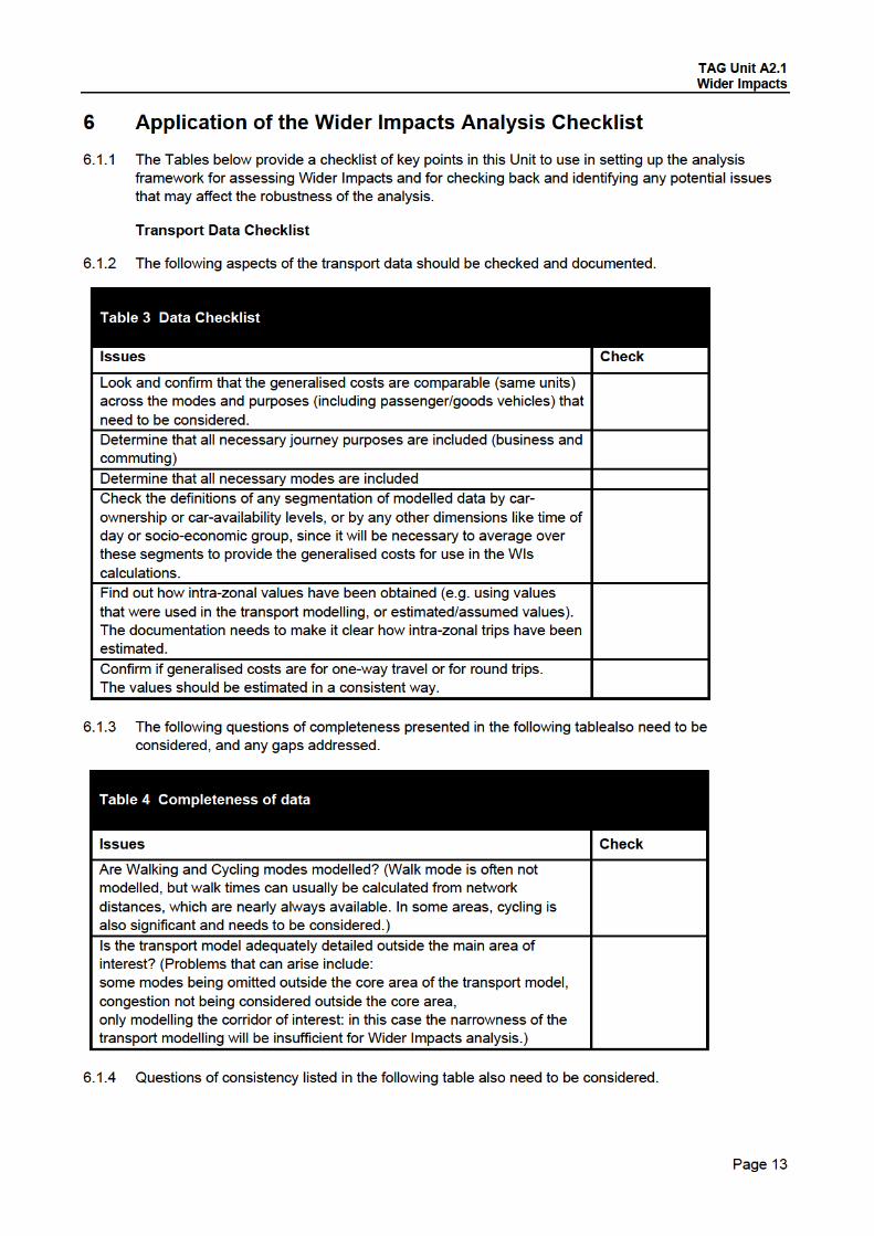
6.1.1 The Tables below provide a checklist of key points in this Unit to use in setting up the analysis

framework for assessing Wider Impacts and for checking back and identifying any potential issues

that may affect the robustness of the analysis.

Transport Data Checklist

6.1.2 The following aspects of the transport data should be checked and documented.

Table 3 Data Checklist

Issues Check

Look and confirm that the generalised costs are comparable (same units)

across the modes and purposes (including passenger/goods vehicles) that

need to be considered.

Determine that all necessary journey purposes are included (business and

commuting)

Determine that all necessary modes are included

Check the definitions of any segmentation of modelled data by car-

ownership or car-availability levels, or by any other dimensions like time of

day or socio-economic group, since it will be necessary to average over

these segments to provide the generalised costs for use in the WIs

calculations.

Find out how intra-zonal values have been obtained (e.g. using values

that were used in the transport modelling, or estimated/assumed values).

The documentation needs to make it clear how intra-zonal trips have been

estimated.

Confirm if generalised costs are for one-way travel or for round trips.

The values should be estimated in a consistent way.

6.1.3 The following questions of completeness presented in the following tablealso need to be

considered, and any gaps addressed.

Table 4 Completeness of data

Issues Check

Are Walking and Cycling modes modelled? (Walk mode is often not

modelled, but walk times can usually be calculated from network

distances, which are nearly always available. In some areas, cycling is

also significant and needs to be considered.)

Is the transport model adequately detailed outside the main area of

interest? (Problems that can arise include:

some modes being omitted outside the core area of the transport model,

congestion not being considered outside the core area,

only modelling the corridor of interest: in this case the narrowness of the

transport modelling will be insufficient for Wider Impacts analysis.)

6.1.4 Questions of consistency listed in the following table also need to be considered.

TAG Unit A2.1 Wider Impacts

Page 14

Table 5 Consistency of data

Issues Check

Do the differences in generalised costs show reasonable patterns, in

particular:

Do generalised costs generally increase for longer journeys?

Do the differences in generalised costs across modes look reasonable?

What, if any, generalised costs are supplied where the mode data is not

immediately available from the model?

Do the generalised costs change in the expected directions if transport

supply improvements are introduced?

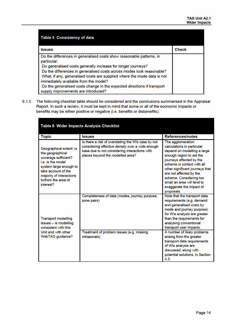
6.1.5 The following checklist table should be considered and the conclusions summarised in the Appraisal

Report. In such a review, it must be kept in mind that some or all of the economic impacts or

benefits may be either positive or negative (i.e. benefits or disbenefits).

Table 6 Wider Impacts Analysis Checklist

Topic Issues References/notes

Geographical extent: is

the geographical

coverage sufficient?

i.e. is the model

system large enough to

take account of the

majority of interactions

to/from the area of

interest?

Is there a risk of overstating the WIs case by not

considering effective density over a wide enough

base due to not considering interactions with

places beyond the modelled area?

The agglomeration

calculations in particular

depend on modelling a large

enough region to set the

journeys affected by the

scheme in context with all

other significant journeys that

are not affected by the

scheme. Considering too

small an area will tend to

exaggerate the impact of

proposals.

Transport modelling

issues – is modelling

consistent with this

Unit and with other

WebTAG guidance?

Completeness of data (modes, journey purpose,

zone pairs)

Note that the transport data

requirements (e.g. demand

and generalised costs by

mode and journey purpose)

for WIs analysis are greater

than the requirements for

analysing conventional

transport user impacts.

Treatment of problem issues (e.g. missing

intrazonals)

A number of likely problems

arising from the greater

transport data requirements

of WIs analysis are

discussed, along with

potential solutions, in Section

4.3.

TAG Unit A2.1 Wider Impacts

Page 19

Appendix A Functional Urban Regions (FURs)

A.1.1 Figure A1 below identifies the Functional Urban Regions in England. This Unit is also accompanied

by a worksheet to use for checking whether the area (designated as either a Census Area Statistic

ward(s) or Local Authority District(s)) in which a scheme is located lies within a single FUR or

multiple FURs.

Figure A1 Functional Urban Regions

Background Information on Designation of Functional Urban Regions

A.1.2 Each FUR is constructed by firstly defining a core and then identifying a corresponding commuting

field (or hinterland) for that core. Census Area Statistics (CAS) wards are used as building blocks for

both the core and commuting field.

A.1.3 The core is defined by a minimum working population (of 60,000) together with a minimum job

density (of 7 jobs per hectare) for a ward. This is to reflect the fact that agglomeration impacts are

TAG Unit A2.1 Wider Impacts

Page 20

most significant for transport schemes located within, or near, large and dense employment centres.

A core can be made up of one or more wards. The methodology largely follows that of the Group for

European Metropolitan Areas Comparative Analysis also know as GEMACA approach.

A.1.4 For the commuting field, the wards surrounding a core are examined. If more workers in the ward

commute to that core than to any other core and a minimum 10% of the working population

commutes to that core, then the ward is added to that core’s commuting field. The use of a

commuting field reflects the fact that agglomeration is influenced by the level of economic interaction

between different areas, with stronger interaction delivering greater potential for agglomeration

impacts. Wards are examined in a contiguous fashion building outwards from each core, with wards

being added to a core’s commuting field until a ward does not meet the two commuting thresholds

set. Again, the methodology largely follows that of the GEMACA approach.

A.1.5 The core plus its commuting field then constitutes a FUR13. All cores across England are identified

and commuting fields then constructed around these cores.

13 Measures of commuting and workplace population at CAS ward level are ONS figures from the 2001 census.

TAG Unit A2.1 Wider Impacts

Page 25

Appendix C Sectoral Aggregation Information from UK SIC(92) 2

digit Classification

C.1.1 The table below provides the necessary sectoral aggregation information from UK SIC(92) 2 digit

classification to the four sectors used in the Wider Impacts estimates

Table C1 Sectoral aggregation

SIC(92)

2 digits Description Sector Group

15 Food Manufacturing

17 Textile Manufacturing

18 Apparel Manufacturing

19 Leather Manufacturing

20 Wood Manufacturing

21 Paper Manufacturing

22 Publishing Manufacturing

24 Chemical Manufacturing

25 Plastic Manufacturing

26 Mineral Manufacturing

27 Basic Metals Manufacturing

28 Fabricated Metals Manufacturing

29 Machinery Other Manufacturing

30 Office Machinery Manufacturing

31 Electrical Machinery Other Manufacturing

32 TV Communication Manufacturing

33 Optical Precision Manufacturing

34 Vehicles Manufacturing

35 Other Transport Manufacturing

36 Furniture and other manufacturing

products not elsewhere classified Manufacturing

45 Construction Construction

50 Motor Trade Consumer Services

51 Wholesale Consumer Services

52 Retail Consumer Services

55 Hotels Restaurants Consumer Services

60 Land Transport Consumer Services

61 Water Transport Consumer Services

63 Travel Support Consumer Services

64 Post Telecom Consumer Services

65 Financial Producer Services

66 Insurance Producer Services

67 Auxiliary Financial Producer Services

71 Machinery Renting Producer Services

72 Computer Services Producer Services

73 R&D Producer Services

74 Other Business Services Producer Services

TAG Unit A2.1 Wider Impacts

Page 35

D.1.25 The final labour market estimate may be positive or negative, depending on the impact of the

transport scheme on generalised cost, employment and residential location across the area.