TAC X4.1 Quick Start - Bruxton Corporation reads event tables written by TAC in order to calculate histograms and perform fitting. Package This package contains TAC X4.1, an experimental

TAC X4.1 Quick Start

Quick Start

This Quick Start is intended to allow you to use TAC asquickly as possible. It provides basic information needed touse the product. For more information, please see the manual.

The TAC package contains two programs, TAC andTACFit. TAC reads recorded data and performs event detec-tion. TACFit reads event tables written by TAC in order tocalculate histograms and perform fitting.

Package

This package contains TAC X4.1, an experimental ver-sion of TAC that supports the Hidden Markov Method of sin-gle-channel analysis, in addition to the threshold idealizationmethod supported by earlier versions of TAC.

You should use TAC X4.1 unless you want to run TACon a 68k Macintosh, which is supported by TAC X4.1. Thispackage also contains TAC V3.0, an older release of TAC.TAC V3.0 is contained in the TAC V3.0.4 folder on the .

TAC X4.1

TAC X4.1 is an experimental release of TAC designed toprovide investigators with experience using the HiddenMarkov Method of single-channel analysis.

TAC X4.1 includes two algorithms, from the labo-ratory of Dr. Fred Sigworth at Yale University and from Qin,Auerbach, and Sachs at Buffalo. Both methods are pub-licly available. TAC provides data selection and conversion, aconvenient user interface, and analysis of results.

Support for analysis is provided through an email

list at ‘[email protected]’. To subscribe to the list, sendemail to ‘[email protected]’ containing the lines:

subscribe hmmstop

The ‘stop’ is necessary to prevent the ‘list-request’ robotfrom processing additional text, such as your email signature.The subject of the email message can be empty.

To remove yourself from the list, send an email messageto ‘[email protected]’ containing the lines:

unsubscribe hmmstop

If you want to communicate with other users of the techniques, send email to ‘[email protected]’.

Changes from TAC V3.0

TAC X4.1 supports Windows /, Windows /, and Macintosh PowerPC systems, and contains many fea-tures not present in earlier versions of TAC, as described inthe following sections.

TAC: Files

TAC can open multiple data files simultaneously. Thefiles are displayed in the Filelist window. The Dataset windowdisplays information about the selected file. The group, sweep,and series entries show navigation information from the datafile. For Pulse users, this allows you to easily identify a spe-cific sweep.

Section

TAC .

TACFit .

Common Features .

Yale HMM .

SUNY Buffalo HMM .

http://www.bruxton.com Bruxton Corporation

TAC: Events

In TAC, the Data window and the Events window aresynchronized. You can select an event in one window, and itwill be selected in the other.

TAC: Selecting Data

In TAC, you can now select multiple segments within asweep for analysis. � Selecting Data, p. .

TACFit: Tag Field

In TACFit, you can use the ‘Tag’ field of the event tablefor more complex selection. Use Level: Tag Value to set thetag value for selected levels. For example, you can select levelsby one set of criteria, set the tag value, then use that tag valuein another selection. The Level: Tag Value dialog sets the tagvalue of all events making up the level.

TACFit: Cluster Analysis

In TACFit, the tag value can assist in cluster analysis.In the Settings: Events dialog, you can specify how

TACFit determines the tag value for a level. The default set-ting is ‘Event’, so the tag value for a level is set from the tagvalue of the event. Instead of ‘Event’, you can specify ‘Closingcount’, so the tag value for a level represents the number ofclosings in the burst that resulted in the level. If the level wasgenerated from a single event, the closing count is zero.

You can use the tag value in several ways. For example,you can use it to select only openings that are part of a burst.To do this, use Settings: Events to set the level tag value to‘Closing count’, and set the burst resolution appropriately.Now the tag value of each level is the number of closings inthe burst. Next, use Level: Tag Value to set the tag value ofeach event to the tag value of the associated level. Now thetag value of each event is the number of closings in the associ-ated burst. Finally, change Settings: Events to the default set-ting of ‘Event’, so the level tag value is the same as the eventtag value, and set the burst resolution to zero, so events arenot collapsed into bursts. Now the tag value of each level isthe number of closings in the associated burst.

Manuals

The manuals are provided in Adobe Acrobat ( ) for-mat on the , along with the Acrobat Reader. For moreinformation about Acrobat, see http://www.adobe.com.

For this release of TAC, the supplied manual describesTAC V3.0, an older version of the product.

Support

For product support, contact Bruxton Corporation at:

email: [email protected]@bruxton.com

: http://www.bruxton.com

Voice: 206 782-8862: 206 782-8207

Mail: Bruxton CorporationPO Box 17904Seattle WA 98107-1904USA

Installation

Hardware Key (Dongle)

TAC requires a hardware key to operate. If you receivedthis version of TAC as an upgrade from a previous version,you should use your existing hardware key.

Windows

For Windows users, install the hardware key on your par-allel port or port. You must also install the associateddriver. To run the installer for the dongle, double click on theRainbowSSD.exe file located in the Rainbow folder on yourTAC . For example, if your drive is ‘d’, your path to thefile would be:

C:\> d:\Rainbow\RainbowSSD.exe

Then, follow the instructions in the installer to completethe installation.

Macintosh

For Macintosh users, either a or an dongle maybe supplied. The dongle is used on and earlier Macin-tosh systems The dongle is used on and later Macin-tosh systems.

If you have a dongle on the Macintosh, you mustinstall the appropriate system extension. The TAC distribu-tion includes a folder ‘Rainbow’ containing the folder ‘Exten-sions’. Move the contents of this ‘Extensions’ folder into the‘Extensions’ folder of your Macintosh ‘System Folder’, andrestart your Macintosh. The dongle system extension will


then run.

Setup

Run the installation programs listed in the table.

TAC X4.1 is supported only on PowerPC Macintosh sys-tems. TAC X4.1 is not supported on 68k Macintosh systems.

The Qin, Auerbach, and Sachs software runs under Win-dows / and Windows . It does not run on Apple Mac-intosh systems.

Platform Install

Microsoft WindowsRainbow\RainbowSSD.exesetup.exe

Apple PowerMacTAC.seaRainbow:Extensions


TAC

Starting TAC

Start the TAC program. TAC will start with the sameparameter settings and arrangement of windows as it had atthe end of the previous run. This information is stored in thepreferences file.

Viewing Data

This section explains how to open a data file using TACand view the data in the file.

File: Settings

When TAC starts, it displays the File Settings dialog.� Figure .

Select the type of data file to read.

File: Open Data

TAC displays the standard file open dialog. � Figure .

Select the data file to read, and press Open. TAC willopen the data file. Depending on the type of the data file,TAC may present another dialog asking for additional infor-mation.

If the file you selected has multiple data channels, TACrequires you to select the channel you want to analyze. Toview and analyze data from a different channel, you mustclose the file and open it again. You cannot change channelswhile you have a file open.

Screen Layout

After TAC opens the data file, it displays the Datasetwindow and the Data window.

The Dataset window displays the groups, series, andsweeps in the file. The title of the Dataset window is the nameof the acquired data file.

Section

Starting TAC .

Viewing Data .

Selecting Data .

Leak Subtraction .

Detecting Events .

Saving the Event Table .

Figure 1: File Settings dialog

Figure 2: File Open dialog


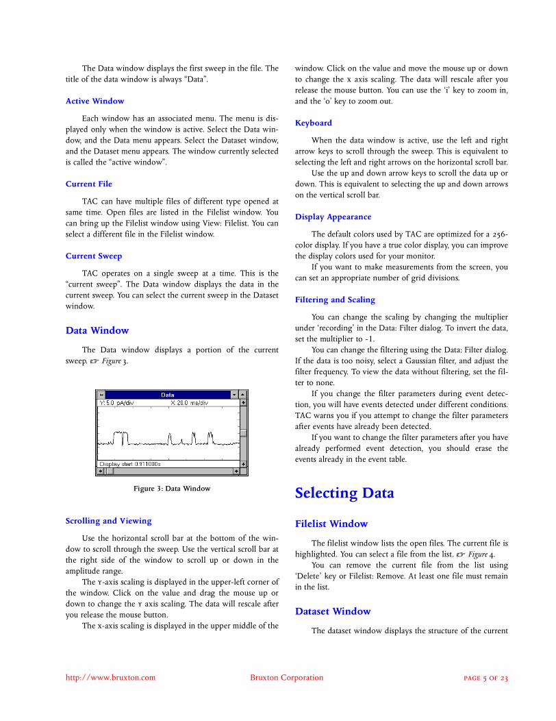
The Data window displays the first sweep in the file. Thetitle of the data window is always “Data”.

Active Window

Each window has an associated menu. The menu is dis-played only when the window is active. Select the Data win-dow, and the Data menu appears. Select the Dataset window,and the Dataset menu appears. The window currently selectedis called the “active window”.

Current File

TAC can have multiple files of different type opened atsame time. Open files are listed in the Filelist window. Youcan bring up the Filelist window using View: Filelist. You canselect a different file in the Filelist window.

Current Sweep

TAC operates on a single sweep at a time. This is the“current sweep”. The Data window displays the data in thecurrent sweep. You can select the current sweep in the Datasetwindow.

Data Window

The Data window displays a portion of the currentsweep. � Figure .

Scrolling and Viewing

Use the horizontal scroll bar at the bottom of the win-dow to scroll through the sweep. Use the vertical scroll bar atthe right side of the window to scroll up or down in theamplitude range.

The -axis scaling is displayed in the upper-left corner ofthe window. Click on the value and drag the mouse up ordown to change the axis scaling. The data will rescale afteryou release the mouse button.

The -axis scaling is displayed in the upper middle of the

window. Click on the value and move the mouse up or downto change the axis scaling. The data will rescale after yourelease the mouse button. You can use the ‘i’ key to zoom in,and the ‘o’ key to zoom out.

Keyboard

When the data window is active, use the left and rightarrow keys to scroll through the sweep. This is equivalent toselecting the left and right arrows on the horizontal scroll bar.

Use the up and down arrow keys to scroll the data up ordown. This is equivalent to selecting the up and down arrowson the vertical scroll bar.

Display Appearance

The default colors used by TAC are optimized for a -color display. If you have a true color display, you can improvethe display colors used for your monitor.

If you want to make measurements from the screen, youcan set an appropriate number of grid divisions.

Filtering and Scaling

You can change the scaling by changing the multiplierunder ‘recording’ in the Data: Filter dialog. To invert the data,set the multiplier to -1.

You can change the filtering using the Data: Filter dialog.If the data is too noisy, select a Gaussian filter, and adjust thefilter frequency. To view the data without filtering, set the fil-ter to none.

If you change the filter parameters during event detec-tion, you will have events detected under different conditions.TAC warns you if you attempt to change the filter parametersafter events have already been detected.

If you want to change the filter parameters after you havealready performed event detection, you should erase theevents already in the event table.

Selecting Data

Filelist Window

The filelist window lists the open files. The current file ishighlighted. You can select a file from the list. � Figure .

You can remove the current file from the list using‘Delete’ key or Filelist: Remove. At least one file must remainin the list.

Dataset Window

The dataset window displays the structure of the current

Figure 3: Data Window


file. � Figure .

Navigation

The current sweep is highlighted in the Dataset window.You can either use mouse to select other sweeps or use up anddown arrow keys to navigate through the sweeps.

Each time you select a new sweep, the sweep is read andprocessed. The time this takes depends on the length of thesweep and the speed of your computer.

Continuation Sweep

If you see a continuation sweep in the dataset window, asweep in the data file was too large for the sweep buffer, soTAC split it into several sweeps for processing. You can set thesize of the memory buffer TAC uses for sweeps using File:Settings. Any change you make takes effect the next time youstart TAC.

TAC also creates continuation sweeps if you used eventscreening during data acquisition. In this case, each sweep orcontinuation sweep represents a segment of recorded data.

Selected Segments

You can select data to analyze. When you open a datafile, you can specify that only a specific segment of eachsweep be selected. If you do not do so, the entire contents ofeach sweep are selected. Each selected segment is shown witha vertical marker at the beginning and end of the segment.� Figure .

You can adjust the selections with the mouse. To add anew selection, double-click at the top edge of the data graph.Two vertical markers will appear. Move them into positionwith the mouse. If you add a new selection within an existing

selection, the existing selection will split into two. To delete aselection, double-click on a vertical marker.

Event detection is performed only within selected seg-ments.

Selection Window

The data selections are shown in the Selection window.� Figure .

Using commands under Data: Selection, you can eitherdeselect a sweep or all sweeps, or restore the data selection ofa sweep or all sweeps to the selection when you first open thedata file(s). You can also apply the selection of the currentsweep to a specified number of following sweeps.

Loaded Data

Some operations, such as the Yale and the selecteddata histogram, require that data be loaded in memory. Toload the selected data in memory, use Selection: Load. Theloaded data will not be automatically updated when you makechanges to the data selection. You must perform Selection:Load again to update the loaded data.

Events Window

The events window displays detected events. When youfirst open a data file, it will be empty. � Figure .

Figure 4: Filelist window

Figure 5: Dataset window

Figure 6: Relevant segment

Figure 7: Selection window


Selection Histogram

This section explains how to use TAC to obtain cumula-tive amplitude histogram of the selected data.

Loaded Data

The cumulative histogram is computed based on theloaded data. To load the selected data, use Selection: Load.The Selection Histogram divides a range of currents into his-togram bins, and counts the number of samples in the loadeddata that fall in each bin.

Fitting

You can fit the Selection Histogram to a sum of gauss-ians. Double-click within the histogram window or use Selec-tion Histogram: Manual Fit. Move the large box in the middleof the component to change the amplitude and current. Movethe small box at the edge of the component to change thewidth of the gaussian.

Double-click on the axis to obtain more fit compo-nents. Double-click on the large box of a fit component toremove it.

Manually set the number of fit components and approxi-mate starting values for fitting. Then use Selection Histogram:Automatic Fit to perform a maximum-likelihood fit.

Leak Subtraction

If your data is recorded as responses to a stimulus, theacquired data will contain capacitive transients that must beremoved before event detection. This is called “leak subtrac-tion”. You can use TAC to perform leak subtraction.

Technique

To subtract the leak current from each sweep, you firstbuild a “leak template”, then subtract this template from eachsweep. A leak template is essentially a sweep that containsonly passive responses to the stimulus.

To construct the leak template, select sweeps (or portions

of sweeps) that contain no channel openings, and averagethem. Although averaging provides a more accurate leak tem-plate, it also increases the noise. You can remove the noise byfitting segments of the leak template to analytical functions.

To perform leak subtraction, both the leak template andthe sweeps to be analyzed must have passive responses of thesame amplitude. This will not be the case if the stimuli them-selves vary in amplitude. TAC allows you to scale both thedata and the leak template to match passive responses.

Forming the Template

Use Data: Leak Settings to set the scaling. Usually the“data to template” and “template to data” scaling will both be1 (one). You can change the scaling at any time.

Use Data: Leak Correction to bring up the leak templatecontrol panel. Use “Clear” to clear any existing leak template.Make sure that “Correct” is not checked.

Move to the sweeps to be included in the leak template,either using the Dataset window or the “Previous” and “Next”buttons in the Data: Leak Correction control panel. At eachsweep to be included, use “Add” to add the sweep to the leaktemplate. The leak template appears in the Data window.

If you cannot see the leak template, check the Data: Dis-play dialog to ensure that display of the leak template isenabled.

Channel Activity

You may find that you do not have sufficient acquiredsweeps without channel activity to form a good leak template.In this case you can add selected segments of a sweep to theleak template.

Move the relevant segment markers to select a portion ofa sweep containing no channel openings, not a passiveresponse. When you select Add in the Data: Leak Correctiondialog, only the relevant segment will be added.

Do not be concerned if your leak template has “holes”without data. This can be corrected by fitting the template.� Figure .

Figure 8: Events window

Figure 9: Leak template with missing data


Fitting

You can reduce noise in the leak template and eliminate“holes” using fitting. Move the relevant segment markers toselect the segment to be fit. Then use the fit buttons in theData: Leak Correction dialog. “Fit Exp” fits the relevant seg-ment to an exponential. “Fit Ramp” fits the relevant segmentto a ramp. “Fit Level” fits the relevant segment to a fixed level.Fit to an exponential is least-squares.

Using the Template

To use the leak template, select “Correct” in the Data:Leak Correction dialog. All displayed data will have the leaksubtracted.

You may want to eliminate display of the leak templateto simplify viewing the corrected data. Use the Data: Displaydialog and disable display of the leak template.

Scaling

If the stimuli used to generate the leak template are ofdifferent amplitude than those used to generate sweeps foranalysis, as is the case in / subtraction, adjust the scaling inData: Leak Settings. For example, suppose you acquired foursweeps for leak subtraction, each with a stimulus amplitude of

the stimulus used for acquisition ( ), you would

set the “Template to data” scaling factor to .

Offsets

You need not use leak subtraction to remove baseline off-set. TAC ignores the baseline offset when performing eventdetection.

Detecting Events

This section explains how to use TAC to detect events inthe acquired data.

Technique

TAC uses a 50% threshold technique to detect events. Anideal transition is shown in figure .

Transition Time

The transition time occurs at the half-amplitude of thetransition. TAC determines this point for each transition. Itdoes not use the time of threshold crossing as the transitiontime, but rather interpolates to determine the time of crossingthe half-amplitude level, which might be different.

Pre-amplitude and Post-amplitude

TAC determines the pre-amplitude and post-amplitudeby calculating a moving average of data before and after theevent. The accepted pre-amplitude and post-amplitude are theaverage values which have the least variance.

Data: Filter

The Data: Filter dialog controls the parameters used fil-tering recorded data. � Figure .

Digital Filtering

TAC provides digital filtering. If you are not using methods, you should generally use the Gaussian digital filter.The Gaussian digital filter controlled by the filter frequencyparameter. Lower the filter frequency to remove high-fre-quency noise from your data. Raise the filter frequency toallow TAC to recognize short events.

1 4⁄– P 4⁄4–

Figure 10: Ideal Transition

Figure 11: Data Filter dialog

Event amplitude

Post-amplitude

Pre-amplitude

Transition time


Timecourse Resolution

The points-per-wave parameter allows you to control theresolution of the time course. Set this to a higher value (e.g.10-20) to see a detailed time course. Set this to a lower value(e.g. 5) to conserve memory. A detailed time course is usefulwhen resolving short dwell times.

Data: Settings

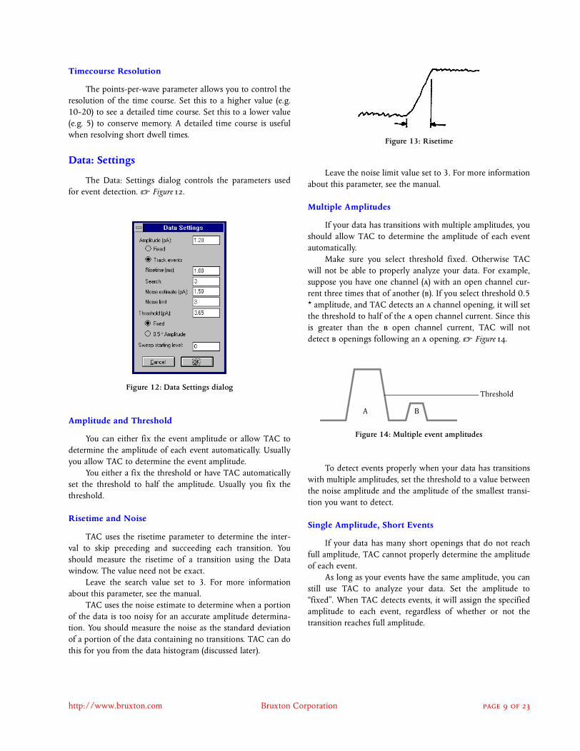
The Data: Settings dialog controls the parameters usedfor event detection. � Figure .

Amplitude and Threshold

You can either fix the event amplitude or allow TAC todetermine the amplitude of each event automatically. Usuallyyou allow TAC to determine the event amplitude.

You either a fix the threshold or have TAC automaticallyset the threshold to half the amplitude. Usually you fix thethreshold.

Risetime and Noise

TAC uses the risetime parameter to determine the inter-val to skip preceding and succeeding each transition. Youshould measure the risetime of a transition using the Datawindow. The value need not be exact.

Leave the search value set to 3. For more informationabout this parameter, see the manual.

TAC uses the noise estimate to determine when a portionof the data is too noisy for an accurate amplitude determina-tion. You should measure the noise as the standard deviationof a portion of the data containing no transitions. TAC can dothis for you from the data histogram (discussed later).

Leave the noise limit value set to 3. For more informationabout this parameter, see the manual.

Multiple Amplitudes

If your data has transitions with multiple amplitudes, youshould allow TAC to determine the amplitude of each eventautomatically.

Make sure you select threshold fixed. Otherwise TACwill not be able to properly analyze your data. For example,suppose you have one channel () with an open channel cur-rent three times that of another (). If you select threshold 0.5* amplitude, and TAC detects an channel opening, it will setthe threshold to half of the open channel current. Since thisis greater than the open channel current, TAC will notdetect openings following an opening. � Figure .

To detect events properly when your data has transitionswith multiple amplitudes, set the threshold to a value betweenthe noise amplitude and the amplitude of the smallest transi-tion you want to detect.

Single Amplitude, Short Events

If your data has many short openings that do not reachfull amplitude, TAC cannot properly determine the amplitudeof each event.

As long as your events have the same amplitude, you canstill use TAC to analyze your data. Set the amplitude to“fixed”. When TAC detects events, it will assign the specifiedamplitude to each event, regardless of whether or not thetransition reaches full amplitude.

Figure 12: Data Settings dialog

Figure 13: Risetime

Figure 14: Multiple event amplitudes

Threshold

A B


Starting Level

A sweep may begin with an open channel. If this occurs,set the Starting Level to the appropriate level for the openchannel. Remember to set the Starting Level back to zerobefore analyzing a different sweep.

Sweep Histogram

You can set both the threshold and the noise estimateautomatically using the sweep histogram. � Figure .

Double-click on the sweep histogram window or selectthe Sweep Histogram: Manual Fit menu item. A fit compo-nent will appear. � Figure .

Move the large box in the middle of the component tochange the amplitude and current. Move the small box at theedge of the component to change the width of the gaussian.

Double-click on the axis to obtain more fit compo-nents. Double-click on the large box of a fit component toremove it.

Manually set the number of fit components and approxi-mate starting values for fitting. Then use Histogram: Auto-matic Fit to perform a maximum-likelihood fit. If the fit isaccurate, you can use Sweep Histogram: Set Detection toautomatically set the event detection threshold and noise esti-mate from the fit.

Data: Detection

Once the parameters are set for event detection, you canbegin detection using the Data: Detection menu item. A dia-log appears with the commands used most frequently in eventdetection. � Figure .

A proposed event appears in the Data window. � Figure.

Interpreting the Proposed Event

The proposed event is displayed as three line segments,one vertical and two horizontal. The horizontal line preced-ing the transition shows the pre-amplitude of the event. Thevertical line shows the transition time. The horizontal line fol-lowing the transition shows the post-amplitude of the event.Each horizontal line segment is one grid division long.

The proposed event is also displayed as text at the bot-tom of the window.

Adjusting the Proposed Event

If the transition should be ignored, use Skip in the Data:Detection dialog or the “” key.

If the transition does not represent a change in levelnumber, for example, a baseline shift, use Jump in the Data:

Figure 15: Sweep histogram

Figure 16: Sweep Histogram with fit component

Figure 17: Data Detection dialog

Figure 18: Data window with proposed event


Detection dialog or the “” key.If any of the segments are incorrect, adjust them using

the mouse. Point at the corresponding line segment and dragthe mouse while keeping the mouse key depressed.

If your data is good and the event detection parametersare set correctly, TAC will detect most events properly. If it isnot able to do so, you will find it much better to adjust thedetection parameters and restart event detection, rather thanmanually adjusting a large number of events.

Commands

To accept the proposed event, use Accept in the Data:Detection dialog or the “ ” key.

Commands in the Data: Detection dialog have equivalentkeyboard keys. For example, the Undo command can beentered as “”. You can use either upper case or lower casekeys, so “f ” and “ ” both mean Accept.

The keys are arranged to make them possible to typewithout moving your hands from the home position on a keyboard.

Mistakes

To remove an accepted event, use Undo in the Data:Detection dialog. The event preceding the proposed eventwill be deleted, and the proposed event will be recalculated.

To remove a large number of events, use the commandsin the Events menu.

Automatic Detection

If your data is good and the event detection parametersare set properly, TAC may be able to automatically detectevents. The commands to perform automatic event detectionare in the Data menu.

You can also perform automatic detection within theentire data file. Use Data: Analyze Remaining or Data: Ana-lyze All.

When using automatic event detection, make sure yourdata is good enough to support automatic event detection.Visually inspect the reconstructed event trace after automaticevent detection. You will never know if TAC made a mistakeunless you verify the results.

Reviewing Results

You can review event detection results by scrollingthrough the data window. You can also scroll through theevents window, which you can bring up using View: Events.Selecting an event in the Events window causes the event toappear in the Data window. Selecting an event in the Datawindow causes the event to appear in the Events window.

Deleting Events

You can delete events in the idealized data trace.You must not be performing event detection. If the Data:

Detection dialog is displayed, you are performing eventdetection. Close the dialog.

To delete events, select an event by clicking with themouse on the vertical line that represents the event transitionin the Data window. The event will change to the proposedevent color. Press the ‘Delete’ key on the keyboard. The tran-sition will disappear. � Figure .

Normally you should delete pairs of events. For example,if TAC encounters a noise spike in your data, it will probablycreate two events. Select each transition and delete it.

To delete a set of events, use commands under Data:Events.

Saving the Event Table

Save the event table using File: Save Events. The firsttime you use File: Save Events after opening a data file, youwill have to specify the file to use to store the event table.Afterwards, when you use File: Save Events, TAC will auto-matically overwrite the existing file with the current eventtable. If you have a long analysis session, you should save yourwork periodically.

To save the event table into an alternate file, use File:Save Events as.

Figure 19: Data window after event deletion


TACFit

Starting TACFit

Start the TACFit program. TACFit will start with thesame parameter settings and arrangement of windows as ithad at the end of the previous run. This information is storedin the preferences file.

Viewing the Event Table

This section explains how to open an event table fileusing TACFit and view the list of events in the file.

Opening an Event Table

TACFit reads event tables produced by TAC.

File: Settings

When TACFit starts, it first displays the File: Settingsdialog. � Figure .

Change the number of event table entries, if necessary,and press Open. TACFit will proceed to the file open dialog.

File: Open

TACFit displays the standard file open dialog. � Figure.

Select the event table file to read, and press Open.TACFit will read the event table.

Processing

After TACFit reads the event table, it computes the asso-ciated levels.

Screen Layout

After TACFit reads the event table file, it displays twowindows, the events window and the levels window. Theevents window displays a list of the events that have beenread into TACFit. The levels window displays a list of ampli-tudes and durations derived from the event table.

Each window has an associated menu. The menu is dis-played only when the window is active. Select the events win-dow, and the events menu will appear. Select the levelswindow, and the levels menu will appear.

Section

Starting TACFit .

Viewing the Event Table .

Examining Data .

Duration Fitting .

Amplitude Fitting .

Stationarity .

Figure 20: File Settings dialog

Figure 21: File Open dialog


Events Window

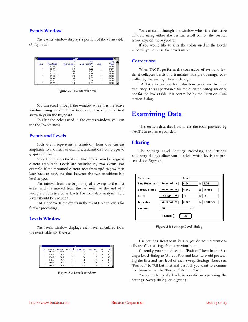
The events window displays a portion of the event table.� Figure .

You can scroll through the window when it is the activewindow using either the vertical scroll bar or the verticalarrow keys on the keyboard.

To alter the colors used in the events window, you canuse the Events menu.

Events and Levels

Each event represents a transition from one currentamplitude to another. For example, a transition from .pA to.pA is an event.

A level represents the dwell time of a channel at a givencurrent amplitude. Levels are bounded by two events. Forexample, if the measured current goes from pA to pA thenlater back to pA, the time between the two transitions is alevel at pA.

The interval from the beginning of a sweep to the firstevent, and the interval from the last event to the end of asweep are both treated as levels. For most data analysis, theselevels should be excluded.

TACFit converts the events in the event table to levels forfurther processing.

Levels Window

The levels window displays each level calculated fromthe event table. � Figure .

You can scroll through the window when it is the activewindow using either the vertical scroll bar or the verticalarrow keys on the keyboard.

If you would like to alter the colors used in the Levelswindow, you can use the Levels menu.

Corrections

When TACFit performs the conversion of events to lev-els, it collapses bursts and translates multiple openings, con-trolled by the Settings: Events dialog.

TACFit also corrects level duration based on the filterfrequency. This is performed for the duration histogram only,not for the levels table. It is controlled by the Duration: Cor-rection dialog.

Examining Data

This section describes how to use the tools provided byTACFit to examine your data.

Filtering

The Settings: Level, Settings: Preceding, and Settings:Following dialogs allow you to select which levels are pro-cessed. � Figure .

Use Settings: Reset to make sure you do not unintention-ally use filter settings from a previous run.

Generally you should set the “Position” item in the Set-tings: Level dialog to “All but First and Last” to avoid process-ing the first and last level of each sweep. Settings: Reset sets“Position” to “All but First and Last”. If you want to examinefirst latencies, set the “Position” item to “First”.

You can select only levels in specific sweeps using theSettings: Sweep dialog. � Figure .

Figure 22: Events window

Figure 23: Levels window

Figure 24: Settings Level dialog


You can distinguish selected and unselected entries in theLevels window by color.

Duration Histogram

View the duration histogram using the View: DurationHistogram menu item. � Figure .

To change the axes of the duration histogram, use theDuration Histogram: Scaling dialog. To change the colors, usethe Duration Histogram: Colors menu.

If the axis extends to negative durations, you can elimi-nate this by specifying that values be constrained to be pos-itive. Negative durations are needed only when fitting first-latency histograms.

If events with short durations appear to be biasedtowards very short durations, the filter frequency may not beset properly in the Duration Histogram: Correction dialog.

If events with short durations appear to be overrepre-sented, perhaps the burst resolution parameters are not setproperly in the Settings: Events dialog.

Amplitude Histogram

View the amplitude histogram using the View: Ampli-tude Histogram menu item. � Figure .

To change the axes of the amplitude histogram, use theAmplitude Histogram: Scaling dialog. To change the colors,

use the Amplitude Histogram: Colors menu.If you are measuring levels using absolute amplitude and

the data contains a single channel with a single open channelcurrent, the histogram will have two peaks, one at the base-line and one at the open channel current. If the histogram hasonly one peak, you may have relative, rather than absolute,level amplitudes selected. This is controlled by the Settings:Events dialog.

Amplitude/Duration Scatter Plot

You can determine if your data has a correlation betweenamplitude and duration using the View: Amplitude/Durationmenu item. � Figure .

To change the axes of the graph, use the Amplitude/Duration: Scaling menu item. To change the colors, use theAmplitude/Duration: Colors menu item.

Statistics

To view basic statistics about the levels, use the View:Statistics menu item. � Figure .

Figure 25: Settings: Sweep

Figure 26: Duration histogram

Figure 27: Amplitude histogram

Figure 28: Amplitude/Duration scatter plot

Figure 29: Statistics window


Like all analysis windows, the statistics window presentsinformation only about the filtered levels.

You can change the colors in the window using the Sta-tistics: Colors menu item.

Duration Fitting

To fit the duration histogram to a theoretical curve, firstperform a manual fit to set the number of terms, then performan automatic fit to optimize the parameters of the theoreticalcurve based on the data.

First-Latency Histogram

To create a first latency histogram, set the “Position” cri-terion in the Settings: Level dialog to “First”.

If you are fitting a first latency histogram, ensure thatnegative durations are allowed on the axis of the histogram.If you are not fitting a first latency histogram, ensure thatdurations are constrained to be positive.

Manual Fit

Bring up the theoretical curve in the duration histogramby double-clicking on the histogram or selecting the DurationHistogram: Manual Fit menu item.

The theoretical curve will appear in the duration histo-gram. � Figure .

The duration fit window will appear with the duration fitparameters. � Figure .

The theoretical curve is a sum of exponential terms. Eachterm is defined by a control point, represented as a square.You can adjust the parameters of a term by dragging the con-trol point vertically to change the weight or horizontally tochange the time constant.

To add a new term to the theoretical curve, double-clickalong the axis. To remove a term from the theoretical curve,double-click on the control point.

Automatic Fit

The automatic fit optimizes the theoretical curve basedon the histogram. The fit uses the maximum likelihood tech-nique.

To perform an automatic fit, select the Duration Histo-gram: Automatic Fit menu item. Make sure that the fit param-eters are set properly in the Duration Histogram: Settingsdialog.

Amplitude Fitting

To fit the amplitude histogram to a theoretical curve, firstperform a manual fit to set the number of terms, then performan automatic fit to optimize the parameters of the theoreticalcurve based on the data.

Manual Fit

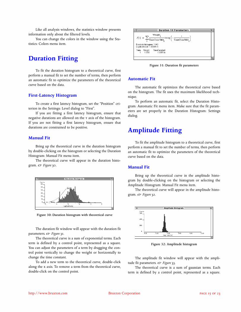
Bring up the theoretical curve in the amplitude histo-gram by double-clicking on the histogram or selecting theAmplitude Histogram: Manual Fit menu item.

The theoretical curve will appear in the amplitude histo-gram. � Figure .

The amplitude fit window will appear with the ampli-tude fit parameters. � Figure .

The theoretical curve is a sum of gaussian terms. Eachterm is defined by a control point, represented as a square.

Figure 30: Duration histogram with theoretical curve

Figure 31: Duration fit parameters

Figure 32: Amplitude histogram


You can adjust the parameters of a term by dragging the con-trol point vertically to change the weight or horizontally tochange the amplitude.

Each control point has an associated standard deviation,represented by a smaller square connected to the controlpoint by a horizontal line. Move the smaller square to changethe standard deviation of the term. � Figure .

To add a new term to the theoretical curve, double-clickalong the axis. To remove a term from the theoretical curve,double-click on the control point.

Automatic Fit

The automatic fit optimizes the theoretical curve basedon the histogram. The fit uses the maximum likelihood tech-nique.

To perform an automatic fit, select the Amplitude Histo-gram: Automatic Fit menu item. Make sure that the fit param-eters are set properly in the Amplitude Histogram: Settingsdialog.

Stationarity

The stationarity plot allows you to view the behavior ofa parameter as a function of time. The time course is filteredto provide an overview. It is most often used to plot the open-channel probability, against time. � Figure .

Filters

The stationarity plot displays the time course of valuesbased on the selected levels. For example, if you are interestedin , use the Settings: Level dialog to select only levels cor-

responding to an open channel.The plot displays the average of data over all selected

sweeps. To display data for a single sweep, use the Settings:Sweep dialog to select only the sweep of interest.

Stationarity: Settings

You control the stationarity plot through the Stationarity:Settings dialog. � Figure .

The type controls the type of weighting. For , use a

weight of 1. This will weight all levels equally with a value of1 (one), so a channel that is always open will result in a valueof 1 and a channel that is always closed will result in a valueof 0.

The stationarity plot also offers weightings by otherparameters, such as amplitude and duration. This allows youto measure changes in level parameters with time.

The tau parameter ( ) adjusts the time constant used forfiltering the time course. The stationarity plot displays no datawithin of the beginning or ending of a sweep.

Figure 33: Amplitude fit parameters

Figure 34: Amplitude histogram showing control points

Po

Figure 35: Stationarity window

Figure 36: Stationarity: Settings

Po

Po

τ

τ 2⁄


Common Features

Data Export

When you have useful results in TAC or TACFit, you canexport them in formats useful for further processing and forpublication.

Text Export

You can save the contents of any window as a text file forfurther processing. For example, you can export the contentsof the data window to perform analysis on the raw data usinganother program.

To export data as a text file, use File: Export Text. Youcan choose to export either only data displayed in the activewindow, or all the underlying data represented by the activewindow. For example, in the case of the data window, you canchoose between the displayed data points and all points in thesweep.

The file export formats are documented so you can inter-pret the files for further processing.

Graphics Export

You can write the contents of any window as a graphicsdata file for printing or publication. For example, you canexport the data window as a graph to show features of youracquired data.

To export a window as a graphic file, use File: ExportGraph. You can also export a window directly to the clip-board using Edit: Copy. If you just want a printed copy of awindow, use File: Print.

When you export a window as a graphic, you have achoice of export formats. For easy export into other applica-tions, use or format. For publication-qualityresults, use or format.

Section

Data Export .


Yale HMM

This section describes the use of the software devel-oped in the laboratory of Dr. Fred Sigworth at Yale University.

The software is included on the , and is distributed atno cost as a convenience. The software is integrated into TAC.

Overview

The Yale HMM software fits a model directly to selecteddata. You choose the data to be analyzed, and specify themodel. The software then iteratively computes the probabilityof the data given the model, and adjusts the model to opti-mize the likelihood of obtaining the data, given the model.

Since the software does not handle voltage or agonistdependencies in the model, all data to be analyzed should berecorded with the same voltage and agonist concentration. Todetermine voltage or agonist dependencies in a model, youmust perform multiple runs with distinct data sets, comparingthe resulting optimized model.

Kinetic Model

You build a kinetic model as a text file. The TAC installa-tion folder contains a sample model file named ‘HMMModel.txt’. Start with this file, and edit it for your needs.

Format

The kinetic model has the following format:

StatesCurrent1 ShotNoise1 InitialProbability1Current2 ShotNoise2 InitialProbability2...

NoiseNoiseControl ControlValueStandardDeviationNoiseStandardDeviationARCoefficients Value1 Value2 Value3 ...

TransitionRateRate11 Rate12 ...Rate21 Rate22 ......

SimulatorNumberOfSweeps SweepsPointsInSweeps PointsSamplingInterval Interval

States

The ‘States’ section lists the current, excess noise, and theprobability of the state at the beginning of a data segment.The current and noise are both measured in amperes, so a typ-ical value for the current might be 1e-11, for 10pA. The cur-rent in each closed state must be zero.

To obtain an initial estimate of the background noise, usethe raw data histogram in TAC. Select a data segment mea-sured while the channel is closed. Fit the amplitude histo-gram. The standard deviation of the current is an estimate ofthe background noise. Remember to convert the value frompA to Amperes. � Sweep Histogram, p. .

To obtain an initial estimate of the excess noise for anopen state, select a data segment measured while the channelis in the state of interest. Fit the raw data amplitude histo-gram. The fit parameters contain the standard deviation of thestate current, which is the total noise in that state. If is the

measured noise in the open state, and is the measured

Section

Overview .

Kinetic Model .

Model Fitting .

Step Response .

Simulator .

σo

σc


background (closed state) noise, , the excess noise in the

state, is computed using . The excess noise is

the value to use in the model. Remember to convert the valuefrom pA to amperes. � Sweep Histogram, p. .

By default, the fitting procedure updates the state currentand initial probability. To specify that a value should be fixed,follow it with an ‘F’, as in ‘18e-12F’.

Noise

‘StandardDevidation’ is the standard deviation of thenoise, in units of amperes. The noise is measured after apply-ing the inverse filter, therefore, it may be substantially greaterthan the noise in the recorded data.

The ‘ARCoefficients’ are the coefficients of the autore-gressive noise model.

If the ‘NoiseControl’ value is non-zero, the other noiseparameters are constrained to their initial values. If ‘NoiseC-ontrol’ is zero, the other noise values are reestimated by thefitting procedure.

If you are not certain of the noise values, set the NoiseC-ontrol to zero, so the parameters are reestimated. Set the Stan-dardDeviation value to the closed channel noise after inversefiltering. You can measure this value using the all-points his-togram in TAC. If you are using a third-order AR model, setthe ARCoefficients to three zero values. The parameters are asfollows:

NoiseControl 0StandardDeviation 0.44e-12ARCoefficients 0 0 0

Initial values for the coefficients can also be deter-mined by fitting closed-channel data to a single-state .

Transitions

The ‘TransitionRate’ section contains the matrix of tran-sition rates. The element at row n column m represents thetransition rate from state n to state m. The rates are expressed

in units of .If you are uncertain as to what initial values to use for the

transition rates, choose values that are approximately the sam-pling rate, that is, the inverse of the sampling interval. Thesampling rate to use as an initial value is not the rate at whichyou acquired your data, but the rate following the applicationof the inverse filter. This rate is shown in the Data: Status dia-log.

The diagonal elements of the transition rate matrix areignored. The diagonal values are automatically set by the pro-gram so the sum across a row is zero.

By default, the fitting procedure updates the transitionrates. To specify that a value should be fixed, follow it with an‘F’, as in ‘50e3F’.

Simulator

The simulator section is used only when creating simu-lated data based on the model.

‘NumberOfSweeps’ is the number of sweeps to be gener-ated.

‘PointsInSweeps’ is the length of each generated sweep,measured as a number of samples.

‘SamplingInterval’ is the sampling interval, measured inseconds.

Model Fitting

Preparing Data

Open the data files of interest. Then disable filtering bysetting the filter type to ‘None’ in Data: Filter.

Select data to be analyzed. By default, all data is selected,unless you choose otherwise when you open a file. You canselect multiple segments in each sweep. � Data Window, p. .

Kinetic Model

Read the kinetic model file into TAC using File: OpenModel.

Inverse Filter

To use a theoretical step response, use the Data: Filterdialog. � Figure .

Select the appropriate inverse filter for your patch-clampamplifier, either ‘Inverse, 4 pole Bessel’ or ‘Inverse, 8 poleBessel’. Specify the recording bandwidth under ‘Recording’and decimation under ‘Inverse filter’. Press the ‘Update’ but-ton in the dialog to generate the inverse filter coefficients.

To use a measured step response, load the cropped stepresponse into the TAC leak template using File: Load Leak.Use the Data: Leak Settings dialog to set the leak templatesample interval. Now in the Data: Filter dialog, set the filtertype to ‘Inverse, User’s’. Specify the decimation under ‘Inversefilter’. Press the ‘Update’ button in the dialog to generate theinverse filter coefficients. � Step Response, p. .

Loading Data

The fit operates on loaded data. Before you performa fit, ensure that the desired data is loaded. To load data, use

σ

σ2 σo2 σc

2–=

s1–


Selection: Load.

Settings

In TAC, the Model: Settings dialog controls the fit-ting. � Figure .

If the fit model is ‘all data simultaneously’, TAC fits asingle model to all the data. If the fit model is ‘by segment’,TAC fits the model to each segment individually. This is use-ful if segments differ in their displayed kinetics.

The calculation mode is either ‘Standard discrete time’ or‘Continuous time’. ‘Standard discrete time’ works well formodels with states with long dwell times. ‘Continuous time’ isbetter for models with short-lived sublevels.

If the baseline is constrained to zero, the algorithmdoes not attempt to fit the baseline. If the baseline is set to‘automatic’, the algorithm estimates a baseline as asequence of linear segments, with one baseline vertex forevery ‘points per vertex’ data points. The baseline algorithmcomputes its own initial estimate of baseline unless a value issupplied under ‘estimate’.

Under ‘Fit’, the tolerance is the change in parameter esti-mates tolerated after an iteration without requiring anotheriteration. ‘Maximum iterations’ is the maximum number ofiterations that TAC performs if the fit does not converge.

The Simulator seed is the initial seed value for the ran-dom number generator.

Fitting

Start the analysis using Model: HMM.TAC updates the Selection window and the Data win-

dow at the end of each iteration. Ensure that a portion ofselected data appears in the Data window so you can see theupdates during fitting.

The fitting terminates automatically either when themaximum number of iterations is reached, or the change inparameter estimates is less than the tolerance. The change inparameter estimates is computed as the square root of the sumof the squares of the fractional parameter value changes.

You can end fitting from the keyboard using the ‘Ctrl’and ‘Break’ keys simultaneously (Windows) or the ‘Com-mand’ and ‘.’ (period) keys simultaneously (Macintosh).

Reviewing

Following the analysis, TAC constructs an idealizedevent list, given the model and the data. You can perform nor-mal TAC event processing using this event list.

The idealized event list has any baseline removed, so asignificant offset may exist between the sampled data and theidealized trace.

Saving

You can save the updated model using File: Export Textwhen the Selection window is the active window. You cansave the event list along with the data selection using File:

Figure 37: Data Filter filter types

Figure 38: Model: Settings dialog


Save Events or File: Save Events As. The saved event file canbe analyzed using TACFit.

Step Response

You can prepare a more accurate inverse filter by measur-ing the step response of your amplifier.

You will measure the step response of your patch-clampamplifier. From this, you will generate an inverse filter thatwill correct your data for the characteristics of your amplifier.You will save the averaged step response, and can use it withall data files acquired under the same filter settings.

Measuring Step Response

The following information was kindly provided by Dr.Sigworth. We have edited it slightly for printing:

“The goal is to acquire the response of the recording sys-tem to a square-wave signal. This response must have verylow noise, so plan to do lots of signal averaging. The idea isto have the headstage input open (no current flowing: nopipette, or pipette in the air not in the bath) and inject currentthrough a capacitor. Here are ways to record the step responsewith various amplifiers.

If you are using an - or -, you can put theamplifier into Test mode, and apply a square wave or pulse tothe Test Input. These patch clamps have a built-in integratorwhich converts the square wave to a triangle wave and appliesit to the input through a capacitor, so there is nothing specialthat you have to do. Best is to use a stimulus pulse generatedby a pulsed-acquisition program. Set the patch-clamp ampli-fier to the gain range that you use in the actual recording,choose the amplitude of the stimulus to give a large but notsaturating response, and average lots ( or ) of sweeps.

If you are using an Axopatch -series amplifier, thereis a test input that feeds your signal directly to a capacitor inthe headstage. To measure the step response with this youneed a triangle wave generator. We did it this way: we set ourWavetek generator to Triggered mode, and triggered it withour pulsed-acquisition program to acquire sweeps.

If you are using an amplifier with no test input, you cando your own capacitive coupling. You need a triangle-wavegenerator. Connect the ground terminal of its output to yoursetup ground. Connect an unshielded wire to the signal out-put and place it somewhere near (a few cm from) your head-stage with the pipette holder attached. You then have a smallcapacitance (say . pF) between the signal wire and thewire in the pipette holder. (Do let the signal wire makeelectrical contact with the head stage input, or you maydestroy the headstage transistors.) When the output of thegenerator is on the order of volts, Hz triangle wave,

the induced current will be on the order of pA (exactly pA peak-to-peak for V peak-to-peak triangle wavethrough . pF). Vary the distance between the wire andpipette holder, or the signal amplitude, to get an appropriate-sized signal.

When you acquire the step response, use the fastest sam-pling you can. Our inverse filter code works best if the stepresponse is sampled twice as rapidly (or more) than youractual acquired data.”

Step Response Processing

In TAC, open the data file containing the recorded stepresponse. Average the response sweeps in the leak template.� Leak Subtraction, p. .

Now export the averaged step response. Make the Datawindow the active window. In the Data: Display dialog, dis-able display of the data, leaving display of the leak templateenabled. Use File: Export Text to save the leak template inExcel format.

Load the saved template into a spreadsheet. Discard thefirst column containing the time. The averaged step responsecontains two transitions: from low to high and from high tolow. Crop the step response to remove the high to low transi-tion. Save the resulting partial single column in text format.� Figure .

Simulator

To use the simulator, read a model file into TAC usingFile: Open Model. Then generate simulated data using File:Simulator. You will have to specify the file in which the simu-lated data is written, as well as a file for the simulated stepresponse.

To view the simulation results, use File: Open Data toopen the simulated data file in TAC as a ‘Bruxton Exchange’file. To specify that input files should be in ‘BruxtonExchange’ format, use the File: Settings dialog.

Figure 39: Step response cropping


SUNY Buffalo HMM

This section describes the use of the software developedby Qin, Auerbach, and Sachs at Buffalo. These programsare collectively called the ‘’ package.

The software is included on the , and is distrib-uted at no cost as a convenience. The Buffalo packageincludes a tutorial in Adobe Acrobat format.

The TAC installation optionally installs the softwareunder Windows / and Windows . The software doesnot run on the Apple Macintosh.

Preparing Data

TAC can export recorded data in the format used by .TACFit can export event lists in the format used by .

Exporting Recorded Data

TAC can export data in the format used by the pro-gram. This means that you can use TAC to open files andselect data for analysis, then transfer the selected data to .

Open the data files of interest. � File: Open Data, p. .Disable filtering. Set the filter type to ‘None’ in Data: Fil-

ter. works best on unfiltered data.Select data to be analyzed. By default, all data is selected,

unless you choose otherwise when you open a file. You canselect multiple segments in each sweep. � Data Window, p. .

Export the data to . Make sure that the Filelist win-dow is the active window. Then select File: Export Binary.Select the file type. The data will be exported in theproper format.

When you export the selected data, you can set the‘leader’ value, used for baseline correction. In TAC, the leaderis expressed in milliseconds. TAC converts this value tomicroseconds for . treats the first and last ‘leader’portion of each segment as baseline, and does not process it.

Save the data selections using File: Save Events. Theempty event table that is saved includes information aboutwhat data is selected. You will need these when you use TAC

review the analysis results.

Exporting Event Lists

TACFit can export the levels table in the format used by. To do this, select File: Save Levels in TACFit. Eachsequence of selected levels is translated to a event cluster.Unselected levels separate clusters.

For example, if you want to analyze clusters of eventswith dwell times less than 100ms, set the Filter: Levels dialogto include only levels with durations from 0ms to 100ms.Levels with longer durations are excluded.

The exported event list should not include jumps in levelnumber. For example, a level at level number 0 can be fol-lowed by a level at level number 1, but should not be fol-lowed directly by a level at level number 2.

Reviewing Results

Use TAC to review an event list generated by . Youcan use TACFit to perform further analysis on this event list,including displaying and fitting histograms.

Reading a QUB Event List

In TAC, restore the data selections using File: OpenEvents. Open the empty event table saved while preparing thedata. This opens the data files and loads the selections.

Read the event list generated by using File: LoadEvents. generates two files needed by TAC, a ‘.dwt’ filelisting the events, and a ‘.tbl’ file containing state currents. InFile: Load Events, specify that you are reading a eventstable, and select the ‘.dwt’ file. TAC automatically reads the‘.tbl’ file.

You now have both the data and the transitions in TAC.You can proceed using normal event analysis.

Section

Preparing Data .

Reviewing Results .


Analyzing Results

In TAC, after you have read the event list generated by, you can save both the data selections and the event listusing File: Save Events. The resulting file can be processed byTACFit. � TACFit, p. .


Documents

TAC X4.1 Quick Start - Bruxton Corporation reads event tables written by TAC in order to calculate histograms and perform fitting. Package This package contains TAC X4.1, an experimental