Tables - Ecology and Society

Appendix 1/10

Junquera, V. and Grêt-Regamey, A. Assessing livelihood vulnerability using a Bayesian network: a case study in northern Laos.

Tables

Table A1.1: Summary of household-level statistics (mean and standard deviation) for each case study area (CSA). The

values reflect conditions in December 2017 unless otherwise noted. Household variable

Oudomsin CSA

(N=60)

Prang CSA

(N=50)

Wilcoxon p-

value*

Age of head of the household 45 (11) 49 (13)

Number of persons (count) 6.7 (2.6) 5.5 (2.2) ***

Number of labor (count) 3.2 (1.3) 2.2 (0.8) ***

Education of head of the household (0 = none, 1 = primary school, 2 =

secondary school, 3 = high school or higher)

0.9 (0.8) 1.1 (0.7) *

Year the household was established in the village 1990 (10) 1990 (9)

Average distance to all household plots, minutes 17 (13) 20 (14)

Average distance to all household plots, kilometers 1.6 (1.0) 1.4 (0.7)

Total income (1000 USD) 4.0 (3.5) 1.2 (1.0) ***

Income from agricultural wages (1000 USD) 1.0 (1.9) 0.1 (0.2) ***

Income from agricultural production (without wages) (1000 USD) 2.3 (2.3) 0.9 (0.8) ***

Net rice income‡ (1000 USD) 0.8 (0.8) 0.7 (0.4)

Income from remittances (1000 USD) 0.002 (0.01) 0.03 (0.2)

Other nonagricultural income (1000 USD) 0.6 (1.3) 0.03 (0.2) ***

Income in 2005 (1000 USD) 1.9 (1.2) 0.4 (0.4) ***

Labor in 2005 (count) 2.7 (1.3) 2.2 (1.0) **

Total agricultural area (ha) 5.6 (2.8) 2.9 (1.2) ***

Rubber area (ha) 4.0 (2.2) 1.1 (0.8) ***

Cardamom area (ha) 0.07(0.2) 0.4 (0.4) ***

Rice paddy area (ha) 0.6 (0.6) 0.5 (0.3)

Paddy land under banana (ha) 0.0 (0.2) 0

Paddy land under sugarcane (ha) 0.9 (1.0) 0 ***

Upland rice area (ha) 0.03 (0.1) 0.5 (0.8) ***

Total rice production (metric tons) 2.7 (2.3) 2.3 (1.2)

Paddy rice production (metric tons) 1.9 (2.0) 1.7 (1.3)

Upland rice production (metric tons) 0.1 (0.3) 0.6 (0.8) ***

Other upland rice production (metric tons) 0.3 (0.7) 0 ***

Rice sold (metric tons) 0.7 (1.5) 0.0 (0.1)

Rice purchased (metric tons) 0.2 (0.5) 0.0 (0.2)

Rubber yield (ton/ha) 1.4 (1.0) 1.4 (0.7)

Paddy rice yield (ton/ha) 3.6 (1.6) 3.8 (1.3)

Upland rice yield (ton/ha) 1.6 (0.4) 1.3 (0.7)

Cardamom yield (ton/ha) na 0.9 (0.3) nd

Rubber farm-gate price (USD/kg) 0.7 (0.1) 0.7 (0.1)

Rice price, nonhulled, farm-gate (USD/kg) 0.3 (0.02) 0.3 (0.03)

Cardamom price (USD/kg) 0.7 (0.6) 0.9 (1.0)

Rubber revenue† (1000 USD/ha) 1.7 (1.6) 0.2 (0.2) nd

Fraction of rubber revenue over total household income† 0.4 (0.3) 0.4 (0.3) nd

Cardamom revenue† (1000 USD/ha) 0.5 (0.4) 0.3 (0.2) nd

Fraction of cardamom revenue over total household income† 0.1 (0.1) 0.5 (0.3) nd

Paddy lease revenue (1000 USD/ha)†† 1.3 (0.9) na nd

Fraction of paddy lease revenue over total household income†† 0.3 (0.3) na nd

Paddy rice revenue (1000 USD/ha)‡‡ 1.1 (0.4) 1.1 (0.3) nd

Notes: A conversion of 8000 LAK = 1 USD is used for 2017 and 2005. nd=not determined. na=not applicable.

†Averaged only over those households having productive cardamom or rubber plantations. Calculated as the factor of the reported yield and farm gate price. ††Averaged only over those households who produce sugarcane in paddy land. Calculated as the factor of yield and farm-gate price (own production) or

plot area and paddy lease price (lease).

‡Theoretical, equal to net rice production (production minus purchases) multiplied by an average rice price of 0.3 USD/kilogram. ‡‡ Theoretical, equal to rice production multiplied by an average rice price of 0.3 USD/kilogram.

* Compares group means using the nonparametric Wilcoxon signed-rank test: *p<0.10, **p<0.05, ***p<0.01.

Appendix 2/10


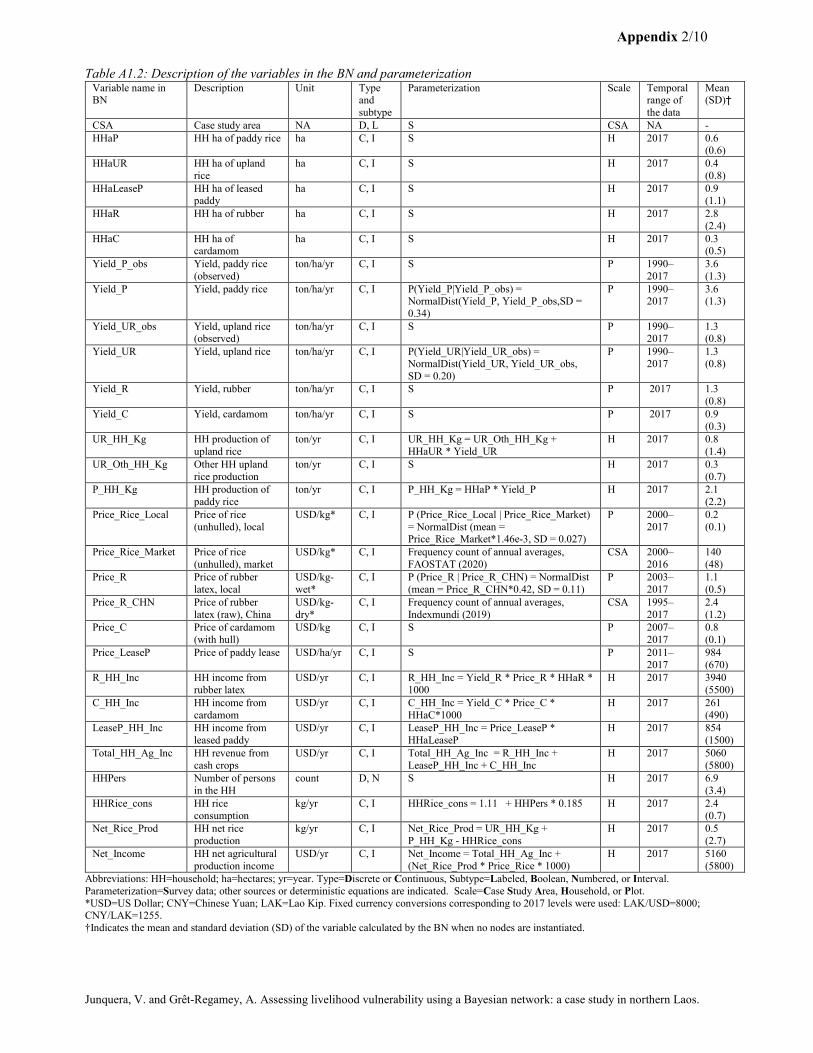
Table A1.2: Description of the variables in the BN and parameterization Variable name in BN

Description Unit Type and

subtype

Parameterization Scale Temporal range of

the data

Mean (SD)†

CSA Case study area NA D, L S CSA NA -

HHaP HH ha of paddy rice ha C, I S H 2017 0.6 (0.6)

HHaUR HH ha of upland

rice

ha C, I S H 2017 0.4

(0.8)

HHaLeaseP HH ha of leased paddy

ha C, I S H 2017 0.9 (1.1)

HHaR HH ha of rubber ha C, I S H 2017 2.8

(2.4)

HHaC HH ha of cardamom

ha C, I S H 2017 0.3 (0.5)

Yield_P_obs Yield, paddy rice

(observed)

ton/ha/yr C, I S P 1990–

2017

3.6

(1.3)

Yield_P Yield, paddy rice ton/ha/yr C, I P(Yield_P|Yield_P_obs) = NormalDist(Yield_P, Yield_P_obs,SD =

0.34)

P 1990–2017

3.6 (1.3)

Yield_UR_obs Yield, upland rice (observed)

ton/ha/yr C, I S P 1990–2017

1.3 (0.8)

Yield_UR Yield, upland rice ton/ha/yr C, I P(Yield_UR|Yield_UR_obs) =

NormalDist(Yield_UR, Yield_UR_obs,

SD = 0.20)

P 1990–

2017

1.3

(0.8)

Yield_R Yield, rubber ton/ha/yr C, I S P 2017 1.3

(0.8)

Yield_C Yield, cardamom ton/ha/yr C, I S P 2017 0.9

(0.3)

UR_HH_Kg HH production of

upland rice

ton/yr C, I UR_HH_Kg = UR_Oth_HH_Kg +

HHaUR * Yield_UR

H 2017 0.8

(1.4)

UR_Oth_HH_Kg Other HH upland

rice production

ton/yr C, I S H 2017 0.3

(0.7)

P_HH_Kg HH production of

paddy rice

ton/yr C, I P_HH_Kg = HHaP * Yield_P H 2017 2.1

(2.2)

Price_Rice_Local Price of rice

(unhulled), local

USD/kg* C, I P (Price_Rice_Local | Price_Rice_Market)

= NormalDist (mean = Price_Rice_Market*1.46e-3, SD = 0.027)

P 2000–

2017

0.2

(0.1)

Price_Rice_Market Price of rice

(unhulled), market

USD/kg* C, I Frequency count of annual averages,

FAOSTAT (2020)

CSA 2000–

2016

140

(48)

Price_R Price of rubber

latex, local

USD/kg-

wet*

C, I P (Price_R | Price_R_CHN) = NormalDist

(mean = Price_R_CHN*0.42, SD = 0.11)

P 2003–

2017

1.1

(0.5)

Price_R_CHN Price of rubber

latex (raw), China

USD/kg-

dry*

C, I Frequency count of annual averages,

Indexmundi (2019)

CSA 1995–

2017

2.4

(1.2)

Price_C Price of cardamom

(with hull)

USD/kg C, I S P 2007–

2017

0.8

(0.1)

Price_LeaseP Price of paddy lease USD/ha/yr C, I S P 2011–

2017

984

(670)

R_HH_Inc HH income from

rubber latex

USD/yr C, I R_HH_Inc = Yield_R * Price_R * HHaR *

1000

H 2017 3940

(5500)

C_HH_Inc HH income from

cardamom

USD/yr C, I C_HH_Inc = Yield_C * Price_C *

HHaC*1000

H 2017 261

(490)

LeaseP_HH_Inc HH income from

leased paddy

USD/yr C, I LeaseP_HH_Inc = Price_LeaseP *

HHaLeaseP

H 2017 854

(1500)

Total_HH_Ag_Inc HH revenue from

cash crops

USD/yr C, I Total_HH_Ag_Inc = R_HH_Inc +

LeaseP_HH_Inc + C_HH_Inc

H 2017 5060

(5800)

HHPers Number of persons

in the HH

count D, N S H 2017 6.9

(3.4)

HHRice_cons HH rice

consumption

kg/yr C, I HHRice_cons = 1.11 + HHPers * 0.185 H 2017 2.4

(0.7)

Net_Rice_Prod HH net rice

production

kg/yr C, I Net_Rice_Prod = UR_HH_Kg +

P_HH_Kg - HHRice_cons

H 2017 0.5

(2.7)

Net_Income HH net agricultural

production income

USD/yr C, I Net_Income = Total_HH_Ag_Inc +

(Net_Rice_Prod * Price_Rice * 1000)

H 2017 5160

(5800)

Abbreviations: HH=household; ha=hectares; yr=year. Type=Discrete or Continuous, Subtype=Labeled, Boolean, Numbered, or Interval.

Parameterization=Survey data; other sources or deterministic equations are indicated. Scale=Case Study Area, Household, or Plot.

*USD=US Dollar; CNY=Chinese Yuan; LAK=Lao Kip. Fixed currency conversions corresponding to 2017 levels were used: LAK/USD=8000; CNY/LAK=1255.

†Indicates the mean and standard deviation (SD) of the variable calculated by the BN when no nodes are instantiated.

Appendix 3/10


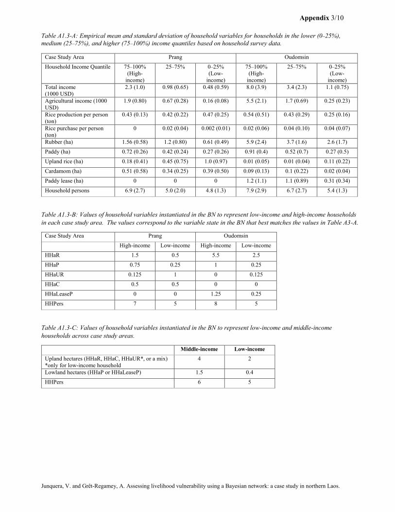
Table A1.3-A: Empirical mean and standard deviation of household variables for households in the lower (0–25%),

medium (25–75%), and higher (75–100%) income quantiles based on household survey data.

Case Study Area Prang Oudomsin

Household Income Quantile 75–100%

(High-

income)

25–75% 0–25%

(Low-

income)

75–100%

(High-

income)

25–75% 0–25%

(Low-

income)

Total income

(1000 USD)

2.3 (1.0) 0.98 (0.65) 0.48 (0.59) 8.0 (3.9) 3.4 (2.3) 1.1 (0.75)

Agricultural income (1000

USD)

1.9 (0.80) 0.67 (0.28) 0.16 (0.08) 5.5 (2.1) 1.7 (0.69) 0.25 (0.23)

Rice production per person

(ton)

0.43 (0.13) 0.42 (0.22) 0.47 (0.25) 0.54 (0.51) 0.43 (0.29) 0.25 (0.16)

Rice purchase per person

(ton)

0 0.02 (0.04) 0.002 (0.01) 0.02 (0.06) 0.04 (0.10) 0.04 (0.07)

Rubber (ha) 1.56 (0.58) 1.2 (0.80) 0.61 (0.49) 5.9 (2.4) 3.7 (1.6) 2.6 (1.7)

Paddy (ha) 0.72 (0.26) 0.42 (0.24) 0.27 (0.26) 0.91 (0.4) 0.52 (0.7) 0.27 (0.5)

Upland rice (ha) 0.18 (0.41) 0.45 (0.75) 1.0 (0.97) 0.01 (0.05) 0.01 (0.04) 0.11 (0.22)

Cardamom (ha) 0.51 (0.58) 0.34 (0.25) 0.39 (0.50) 0.09 (0.13) 0.1 (0.22) 0.02 (0.04)

Paddy lease (ha) 0 0 0 1.2 (1.1) 1.1 (0.89) 0.31 (0.34)

Household persons 6.9 (2.7) 5.0 (2.0) 4.8 (1.3) 7.9 (2.9) 6.7 (2.7) 5.4 (1.3)

Table A1.3-B: Values of household variables instantiated in the BN to represent low-income and high-income households

in each case study area. The values correspond to the variable state in the BN that best matches the values in Table A3-A.

Case Study Area Prang Oudomsin

High-income Low-income High-income Low-income

HHaR 1.5 0.5 5.5 2.5

HHaP 0.75 0.25 1 0.25

HHaUR 0.125 1 0 0.125

HHaC 0.5 0.5 0 0

HHaLeaseP 0 0 1.25 0.25

HHPers 7 5 8 5

Table A1.3-C: Values of household variables instantiated in the BN to represent low-income and middle-income

households across case study areas.

Middle-income Low-income

Upland hectares (HHaR, HHaC, HHaUR*, or a mix)

*only for low-income household

4

2

Lowland hectares (HHaP or HHaLeaseP) 1.5 0.4

HHPers 6 5

Appendix 4/10


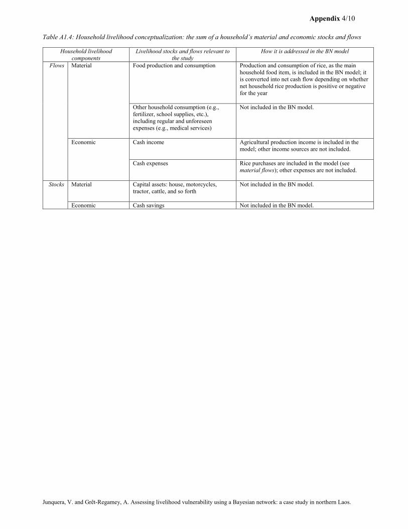
Table A1.4: Household livelihood conceptualization: the sum of a household’s material and economic stocks and flows

Household livelihood

components

Livelihood stocks and flows relevant to

the study

How it is addressed in the BN model

Flows Material Food production and consumption Production and consumption of rice, as the main

household food item, is included in the BN model; it

is converted into net cash flow depending on whether

net household rice production is positive or negative

for the year

Other household consumption (e.g.,

fertilizer, school supplies, etc.),

including regular and unforeseen

expenses (e.g., medical services)

Not included in the BN model.

Economic Cash income Agricultural production income is included in the

model; other income sources are not included.

Cash expenses Rice purchases are included in the model (see

material flows); other expenses are not included.

Stocks Material Capital assets: house, motorcycles,

tractor, cattle, and so forth

Not included in the BN model.

Economic Cash savings Not included in the BN model.

Appendix 5/10


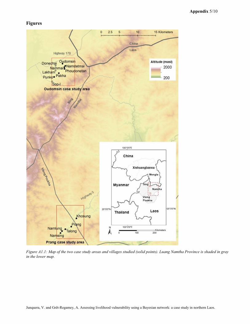
Figures

Figure A1.1: Map of the two case study areas and villages studied (solid points). Luang Namtha Province is shaded in gray

in the lower map.

Appendix 6/10


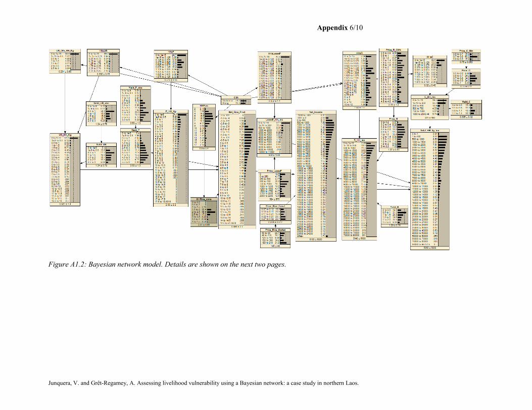
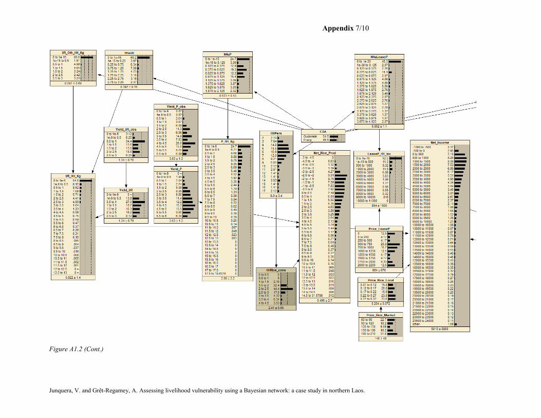
Figure A1.2: Bayesian network model. Details are shown on the next two pages.

Appendix 7/10


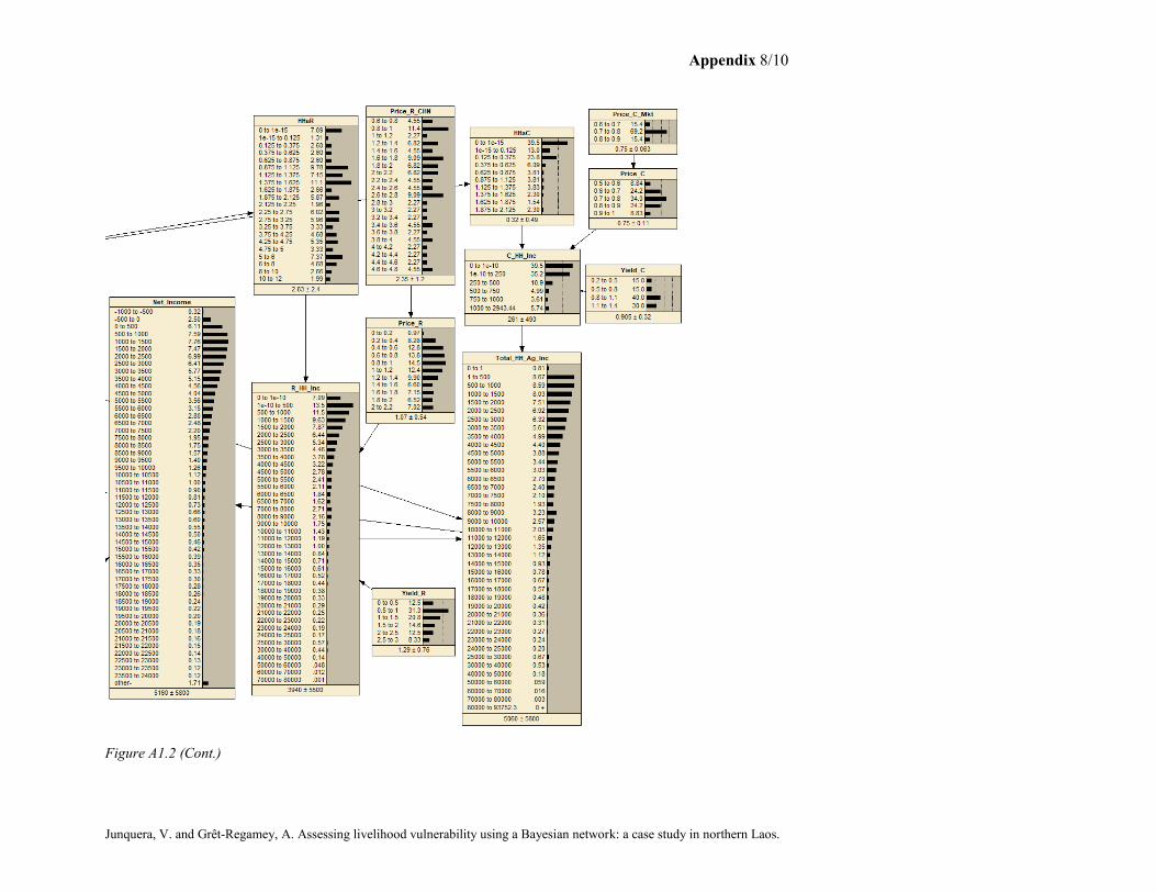
Figure A1.2 (Cont.)

Appendix 8/10


Figure A1.2 (Cont.)

Appendix 9/10


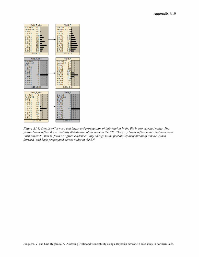
Figure A1.3: Details of forward and backward propagation of information in the BN in two selected nodes. The

yellow boxes reflect the probability distribution of the node in the BN. The gray boxes reflect nodes that have been

“instantiated”, that is, fixed or “given evidence”; any change to the probability distribution of a node is then

forward- and back-propagated across nodes in the BN.

Appendix 10/10


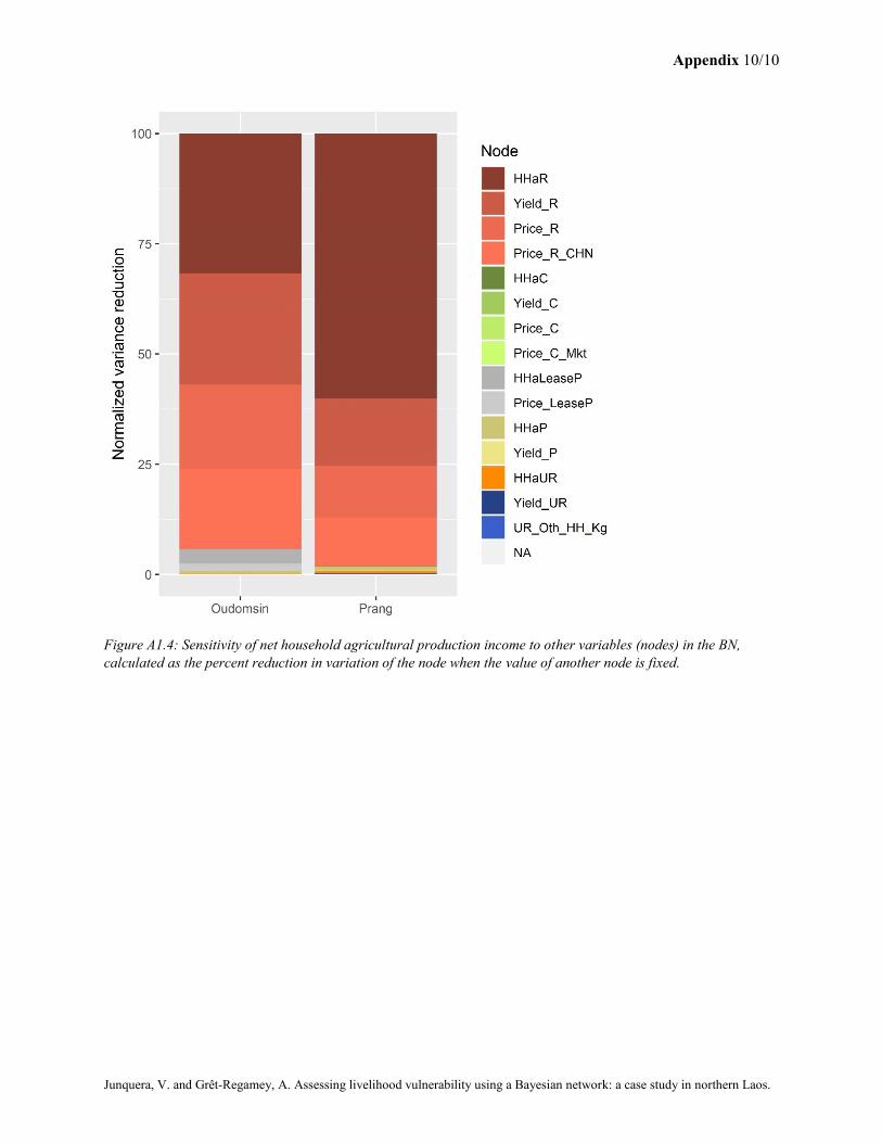
Figure A1.4: Sensitivity of net household agricultural production income to other variables (nodes) in the BN,

calculated as the percent reduction in variation of the node when the value of another node is fixed.

Documents

Tables - Ecology and Society