1

Table of Contents

CAN IRTPRO SPREADSHEET FILES (*SSIG) BE EXPORTED TO SPSS, SAS, STATA, ETC.

FORMATS? 3

CAN IRTPRO BE RUN IN BATCH MODE? 6

HOW CAN ONE IMPORT ASCII FILES TO THE .SSIG FORMAT? 7

DOES IRTPRO IMPOSE ANY PRIORS ON ITEM PARAMETERS BY DEFAULT? 8

CAN IRTPRO HANDLE THE TESTLET RESPONSE THEORY MODEL? 9

CAN IRTPRO DO IRTLRDIF? 9

CAN MAXIMUM LIKELIHOOD SCALE SCORES BE COMPUTED? 9

CAN IRTPRO SCORE PERSONS IN A DATASET CORRECTLY IF SOME ITEMS HAVE ONE

OR MORE CATEGORIES THAT NONE OF THE INDIVIDUALS RESPONDED TO? 9

WHAT IS THE FORMAT OF THE -PRM.TXT PARAMETER OUTPUT / INPUT FILE? 10

IN USING THE MH-RM ALGORITHM, WHEN SHOULD ONE CHECK THE AR VALUE? 12

WHEN IS THE M2 FIT STATISTIC PRINTED? 13

CAN YOU PROVIDE MORE DETAILS REGARDING THE LOGIT(- G) OR THE G

PARAMETER USED IN 3-PL MODELS? 13

WHAT DOES THE "C PARAMETER" REPRESENT IN THE IRTPRO OUTPUT (IF NOT THE

GUESSING PARAMETER)? 14

CAN ONE SPECIFY THE SCALING FACTOR 1.7 IN IRTPRO? 14

IS THERE ANY TECHNICAL INFORMATION AVAILABLE REGARDING THE GPC MODEL

OTHER THAN THE PDF GUIDE? 14

2

WHEN SHOULD PRIORS BE USED IN IRTPRO? 15

HOW CAN ONE SAVE EDITED GRAPHS IN IRTPRO? 15

IS THERE AN EASY WAY TO CHANGE THE APPEARANCE OF MULTIPLE GRAPHS 20

CAN IRTPRO CONDUCT AN IRT ANALYSIS ON REPEATED MEASURES DATA? 25

DOES IRTPRO HAVE THE OPTION OF PRODUCING THE ESTIMATED OBSERVED

SCORES BASED ON THE TEST CHARACTERISTIC CURVE? 25

DOES IRTPRO HAVE THE OPTION OF SUPERIMPOSING THE EMPIRICAL ITEM

RESPONSE CURVE TO THE ESTIMATED ITEM RESPONSE CURVE? 27

CAN YOU PROVIDE MORE DETAILS ON THE TABLES ON PAGES 76 TO 78 AND WHAT

GRAY COLORS MEAN IN THE S-X2 TABLES? 27

CAN IRTPRO COMPUTE STANDARDIZED DISCRIMINATION PARAMETERS? 28

HOW DOES ONE INTERPRET THE COLUMNS OF THE SCORE FILE? 28

3

Can IRTPRO spreadsheet files (*ssig) be exported to SPSS, SAS, STATA,

etc. formats?

This feature is available in IRTPRO 4 and is accomplished as follows:

Use the File, Open option to open an .ssig file

Use the File, Export option to export this file to a different format

Example

Assume we want to export Anxiety14.ssig to the SPSS .sav format. Use the File,

Open option to locate and select this file.

Click the Open button to display the following spreadsheet:

4

Select the File, Export option:

From the drop-down list, select SPSS Data File(*.sav). The Save As dialog enables one

to save the file in any folder. The default folder is the one where the .ssig file is located

and the default name is that of the .ssig file.

5

6

Can IRTPRO be run in batch mode?

There are two ways to run jobs described by existing .irtpro command files; they use the

commands "-Run" and "-RunList":

-Run

To run the command lines in, for example, the file "Spelling.irtpro", assuming it is in the

C:\IRTPRO Examples folder as installed by default, proceed as follows:

"-Run" is used to open IRTPRO and run the analyses described in a single .irtpro

command file. In the Command Prompt window, enter a line of the form (for Windows

7):

"c:\program files (x86)\irtpro21\irtpro" –Run "c:\irtpro

examples\unidimensional\2PL\Spelling.irtpro"

or (for Windows XP):

"c:\program files\irtpro21\irtpro" –Run "c:\irtpro

examples\unidimensional\2PL\Spelling.irtpro"

Notes:

The difference between Windows 7 and XP is the presence or absence of " (x86)" in the

folder name for the IRTPRO executable.

In commands typed in the Command Prompt window, or in .bat files executed there,

double quotes are required around path/file names that contain spaces.

Several lines of the form(s) above can be created one after another in a file with the

extension .bat; then that file can be double-clicked, or invoked in the Command Prompt

window, and the lines will be executed one after another.

The .irtpro files can either be created by the IRTPRO GUI, or appropriately edited

versions of such files, or (possibly) even created by some user-written special-purpose

software.

7

It may be useful to select the -irt.txt, or other .txt file, output in the commands in the

.irtpro file, to yield ASCII files that can be post-processed after a sequence of "batched"

runs.

-RunList

"-RunList" is used to open IRTPRO and run the analyses described in a list of .irtpro

command files; the paths/names for the .irtpro command files are specified as lines of a

.txt file. In the Command Prompt window, enter a line of the form (for Windows 7):

"c:\program files (x86)\irtpro21\irtpro" –RunList "c:\irtpro

examples\unidimensional\2PL_examples.txt"

or (for Windows XP):

"c:\program files\irtpro21\irtpro" –RunList "c:\irtpro

examples\unidimensional\2PL_examples.txt"

in which the file "c:\irtpro examples\unidimensional\2PL_examples.txt" is, for example,

the following four lines:

c:\irtpro examples\unidimensional\2PL\AACL3_21Items.irtpro

c:\irtpro examples\unidimensional\2PL\lsat6.irtpro

c:\irtpro examples\unidimensional\2PL\SelfMon4items2PL.irtpro

c:\irtpro examples\unidimensional\2PL\Spelling.irtpro

Note that no quotes are used around the filenames in the .txt file, even though the paths

contain spaces.

How can one import ASCII files to the .ssig format?

This is accomplished using the utility ascii2ssig.exe. The purpose of this utility is to

convert text data to the IRTPRO .ssig format. By typing in ascii2ssig from the DOS

Command prompt the usage is displayed as illustrated by the screen shot below.

8

As an example, suppose that we want to import the file AACL_21.csv containing 21

items, in the Command Prompt window, enter the line:

ascii2ssig aacl_21.csv 21 /delim=',' /header

Suppose that there are ten similar files called aacl_21_1.csv, aacl_21_2.csv,

aacl_21_3.csv, …, aacl_21_10.csv, then all ten can be converted to .ssig files using

import10.bat:

Does IRTPRO impose any priors on item parameters by default?

IRTPRO does not impose priors on any item parameters or group means/(co) variances

by default. Univariate priors (e.g., beta prior on lower asymptotes) can be activated via

the advanced options dialog box. Univariate priors are supported by all estimation

algorithms.

9

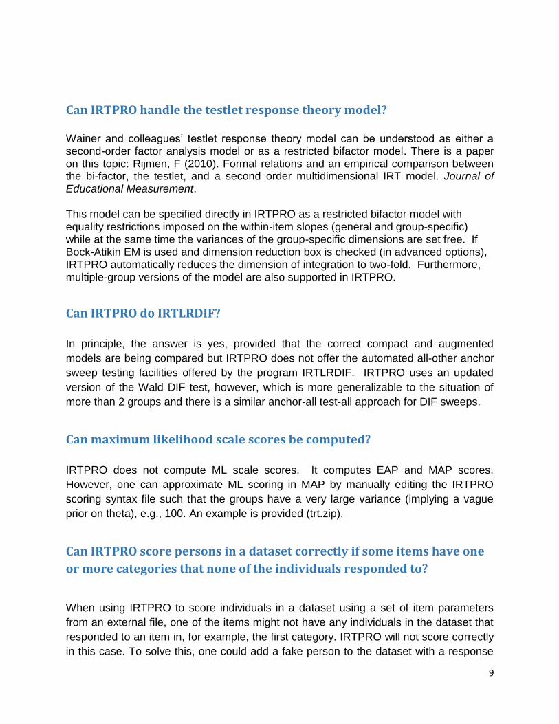
Can IRTPRO handle the testlet response theory model? Wainer and colleagues’ testlet response theory model can be understood as either a second-order factor analysis model or as a restricted bifactor model. There is a paper on this topic: Rijmen, F (2010). Formal relations and an empirical comparison between the bi-factor, the testlet, and a second order multidimensional IRT model. Journal of Educational Measurement. This model can be specified directly in IRTPRO as a restricted bifactor model with equality restrictions imposed on the within-item slopes (general and group-specific) while at the same time the variances of the group-specific dimensions are set free. If Bock-Atikin EM is used and dimension reduction box is checked (in advanced options), IRTPRO automatically reduces the dimension of integration to two-fold. Furthermore, multiple-group versions of the model are also supported in IRTPRO.

Can IRTPRO do IRTLRDIF?

In principle, the answer is yes, provided that the correct compact and augmented

models are being compared but IRTPRO does not offer the automated all-other anchor

sweep testing facilities offered by the program IRTLRDIF. IRTPRO uses an updated

version of the Wald DIF test, however, which is more generalizable to the situation of

more than 2 groups and there is a similar anchor-all test-all approach for DIF sweeps.

Can maximum likelihood scale scores be computed?

IRTPRO does not compute ML scale scores. It computes EAP and MAP scores.

However, one can approximate ML scoring in MAP by manually editing the IRTPRO

scoring syntax file such that the groups have a very large variance (implying a vague

prior on theta), e.g., 100. An example is provided (trt.zip).

Can IRTPRO score persons in a dataset correctly if some items have one

or more categories that none of the individuals responded to?

When using IRTPRO to score individuals in a dataset using a set of item parameters

from an external file, one of the items might not have any individuals in the dataset that

responded to an item in, for example, the first category. IRTPRO will not score correctly

in this case. To solve this, one could add a fake person to the dataset with a response

10

of 1 for that variable so that it would recode people correctly, and then drop the fake

person after scoring the dataset. This is an annoyance, but there is at present (and for

the foreseeable future) no easier solution. When this happens to us, or when we fear it

might happen, we just add as many "fake persons" to the dataset as there are response

categories. For five-category items that's five: If the codes are 1-5, then there's one

that's all 1s, the next is all 2s, etc. up to all 5s.

What is the format of the -prm.txt parameter output / input file?

The –prm.txt output file is a tab-delimited ASCII .txt file that contains one line for each

item and/or group. It is an output file from item calibration runs, and may be used as a parameter input file for stand-along scoring runs.

The tab-delimited format makes it easy for users to edit, or store, by opening it with,

say, Excel.

The one-line-per-item format makes it easy to “mix and match” lines from multiple runs of the program to “assemble” new tests—new combinations of items one may want to score.

Each line contains a variable number of fields, depending on the number of dimensions

and the item response model:

1) For all items / groups, the first field is the label.

2) For all items / groups, the second field is the number of dimensions (“nfac”; an int).

3) For all items / groups, the third field is itemtype: 1 = 3PL, 2 = Graded, 3 = Nominal; 0

means population distribution parameters [mean and (co)variances].

For itemtype = 1, 2, or 3 (these are really items):

4) The fourth field is the number of categories (ncat; an int).

An additional column is added here, if itemtype = 3 (nominal). This is a single integer signaling whether the item is actually to be treated as a GPC item. Recall that GPC is mathematically a special case of the nominal model. If this number is 1, the item is

GPC. If zero, the item is not GPC, hence it is nominal (see Appendix below).

5) For all models, the fifth (set of) field(s) contains nfac real values, the slope(s); these

are the parameters labeled “a” in the “Item Parameter Constraints” window.

For itemtype = 1 (3PL):

6) The sixth field contains a real value, the intercept parameter; these are the

parameters labeled “c” in the “Item Parameter Constraints” window.

7) The seventh field contains a real value, the logit of the guessing parameter; these are

the parameters labeled “g” in the “Item Parameter Constraints” window.

11

8) if (nfac == 1) The eighth field contains a real value, the threshold parameter.*

8/9) if (nfac > 1) The eighth field contains a real value, the guessing parameter; this

value is the ninth field if (nfac == 1).*

*Note: fields marked with * are for the user’s convenience, and will not be used when this file is read as either stating values or as parameter values for scoring.

For itemtype = 2 (Graded):

6) The sixth (set of) field(s) contains (ncat – 1) real values, the intercepts(s) these are

the parameters labeled “c” in the “Item Parameter Constraints” window.

7) if (nfac == 1) The seventh (set of) field(s) contains (ncat – 1) real values, the

thresholds(s).*

*Note: fields marked with * are for the user’s convenience, and will not be used when this file is read as either stating values or as parameter values for scoring.

For itemtype = 3 (Nominal):

6) The sixth field contains an integer, T-matrix type, 0 = Trend, 1 = Identity, 2 = User-

supplied.

7) The seventh (set of) field(s) contains (ncat – 1) real values, the contrast(s) for the

scoring functions. The first of these values is the “1.0” that is always the value of 1;

the rest are subsequent values of the s. [These are the parameters labeled “” in

the “Item Parameter Constraints” window.]

8) The eighth field contains an integer, L-matrix type, 0 = Trend, 1 = Identity, 2 = User-supplied.

9) The ninth (set of) field(s) contains (ncat – 1) real values, the contrast(s) labeled (s) in

the “Item Parameter Constraints” window, for the intercepts.

10-11) if (nfac == 1) The tenth set of fields contain the ncat values of the “ak” parameters, and the eleventh set of fields contain by the ncat values of the “ck” parameters of the old (Bock, 1972) parameterization of the nominal model.*

12) if (nfac == 1) and the model is actually GPC, The twelth set of fields contains the “b” parameter from (one of) Muraki’s paramterization(s), and then the next ncat fields

contain the corresponding “d” parameters—the first “d” is always 0.0.*

*Note: fields marked with * are for the user’s convenience, and will not be used when this file is read as either stating values or as parameter values for scoring.

13) Note: At a later time, the 13th set of fields will contain the elements of any user-

supplied T matrix, followed by the elements of any user-supplied L matrix; that is not

yet implemented.

For itemtype = 0 (these are really group / population parameter values):

12

4) The fourth (set of) field(s) contains nfac real values, the mean(s) ().

5) The fifth (set of) field(s) contains nfac*(nfac+1)/2 real values, the covariance(s), in the

order 1 1, 2 1, 2 2, 3 1, 3 2, 3 3, 4 1, …

6) if (nfac == 1) The sixth field contains a real value, the standard deviation.*

*Note: fields marked with * are for the user’s convenience, and will not be used when

this file is read as either stating values or as parameter values for scoring.

Appendix: The GPC Model

When the model does not contain free scoring function contrasts, the nominal model

(itemtype = 3) is actually a GPC. The way it is done is best illustrated with an example.

In the zip archive, one can find the html output for a 3-item nominal+GPC run. The first

two items are nominal, with the 3rd being GPC. Basically, if the itemtype is 3 (nominal),

the procedure reading the PRM file should expect an additional integer. If it is 0, the

model is not GPC, and hence should be treated as nominal; if 1, the model is GPC.

Here is an excerpt from the -PRM.txt (in the zip archive) output (the first couple of

columns) for items 2 and 3:

Nominal4 1 3 4 0 1.01469 0 1.00000 0.85037

0.80860 0 0.70135 0.46954 0.38907

GPC4 1 3 4 1 1.13518 0 1.00000 0.00000

0.00000 0 0.92548 0.01721 -0.05477

As one can see, the order of PRM listing is the label (indicating one is nominal and the

other is GPC), the number of factors (1-factor in this case), item type (both equal to 3),

the number of categories (both ncat=4), indicator for GPC (item 2 is not GPC and item 3

is GPC), the slope estimate (there is one slope because this is a 1-factor model), the

type of T matrix (scoring function contrast matrix -- this case equal to 0 = Trend), (ncat-

1) scoring function contrast estimates, the type of L matrix (the intercept contrast matrix

-- again 0 = Trend). One thing to note is that for a GPC model, the T matrix type is

always 0, and the first scoring function contrast is always 1.0, and the remaining scoring

function values are all 0. On the other hand, a true nominal model does not have such

restrictions.

In using the MH-RM Algorithm, when should one check the AR value?

13

Check the AR value in the iteration output whenever the MH-RM algorithm is selected.

Ideally, we'd like to keep the AR to something around .25 for models that are high

dimensional (i.e., more than 3 or 4 factors). AR values larger than .25, say, .4 or .5 may

be acceptable if the dimensionality is not too high. If the AR value is too high, the

proposal dispersion constant can be increased. If it is too low, the dispersion constant

should be decreased. If one starts at 1.0 and observe the AR is larger than the target

value, do step-halving. One would stop the iterations, cutting the constant to .5 and

restart the iterations, watch how well the AR does with the new dispersion. If it looks

good, stop, if not, either cut or increase the constant in steps of .1 or .2.

AR is ultimately going to oscillate around a target value due to randomness. An AR of

.28 is probably as good as an AR of .25. The MH chain is going to be just about as

efficient.

See also

Roberts, G.O., & Rosenthal, J.S. (2001). Optimal scaling for various Metropolis-

Hastings algorithms. Statistical Science, 16, 351–367.

When is the M2 Fit statistic printed?

IRTPRO will only print M2 and related statistics when BAEM is used. This is because

we have not been able (yet) to implement a good way to compute the posterior

probabilities and Jacobians and weights needed for M2 with adaptive quadrature

points. So for now, BAEM has all the fit statistics but ADQ and MH-RM has few.

Can you provide more details regarding the Logit(- g) or the g parameter

used in 3-PL models?

The g parameter is the so-called pseudo-guessing (lower asymptote parameter, c

parameter, etc.) in the 3PL model. The logit of g is the parameter that is actually

estimated in IRTPRO because the re-parameterization produces a more nearly

quadratic log-likelihood that is easier for optimization. In other words, we do not

estimate the item guessing probabilities, but rather their log-odds.

Note:

If logit(g) is "z", then g = 1/(1+exp(-z)), which is the usual guessing parameter.

14

What does the "c parameter" represent in the IRTPRO output (if not the

guessing parameter)?

The c parameter is the intercept, which is related to the threshold parameter "b", where:

b = -c/a, and a is the slope.

So the c's are really just -a times the corresponding b (threshold). The intercepts are preferred because they generalize well to multidimensional IRT models.

The critical thing is that we are using the intercept/slope parameterization as opposed to the more typical (but only useful for unidimensional IRT) threshold/slope parameterization. In multidimensional IRT, because there are more than one latent variable in the linear predictor, the closest thing to a threshold would be to transform the c values into thresholds as per Eq (4.9) of M.D. Reckase(2009): Multidimensional Item Response Theory, Statistics for Social and Behavioral Sciences, Springer Science+Business Media. Wirth & Edwards's (2007) paper in Psyc Methods also contains a number of conversion formulae that would work.

Can one specify the scaling factor 1.7 in IRTPRO? IRTPRO does not include the scaling factor D = 1.7 in any equation for any purpose. All trace line equations are written without the 1.7.

Is there any technical information available regarding the GPC model

other than the pdf guide? There are many parameterizations of the GPC model. Some of them are on p. 55 of Thissen, D., Cai, L., & Bock, R.D. (2010 ). The nominal item response model. In M.

Nering & R. Ostini (Eds.), Handbook of polytomous item response theory models: Developments and applications.

The model used in IRTPRO is on p. 59. Conversion to (some of the) GPC parameters is on pp. 60-62. However, because the GPC model has been expressed in many ways, and implemented in many ways in software, the only way to truly figure out translation between IRTPRO and any of the other programs is by cross-checking results.

15

When should priors be used in IRTPRO?

Like Multilog, IRTPRO uses maximum marginal likelihood estimation, which involves no

priors, when doing item parameter calibration, unless the user instructs otherwise. The

user may select item parameter priors through the Priors tab in Advanced Options

dialog box. Or, alternatively, write in the Priors syntax section. Three kinds of prior

densities are supported: Beta, Log-normal, and normal. These univariate priors can be

imposed on any item parameters. However, for the guessing parameter, the normal

prior actually means logit-normal on the logit of guessing probability. The log-normal

prior is mostly meant for the slope parameter in unidimensional models. The beta prior

is supported since people are familiar with the Beta priors in Bilog and Parscale. Due to

the general multidimensional and hierarchical model on top of which IRTPRO is built,

we chose not to assume default priors as does Bilog or Parscale (which have more

limited focuses to unidimensional analysis and can therefore make more assumptions

about the user's intent). Hence, by default, no priors are imposed on any parameter in

IRTPRO. This can cause problems if the 3PL model is used. Unless sample size is

huge, a logit-normal or beta prior on the lower asymptote parameter should be imposed

at the very least.

How can one save edited graphs in IRTPRO?

To illustrate the way that one can save an edited graph, open the file Efficacy.ssig from

the IRTPRO Examples\multidimensional\CFA folder and select the Graphics,

Univariate… option then select NOSAY and VOTING.

Click the OK button to produce the bar charts.

16

Right-click on the NOSAY graph to activate the 2D Chart Control Properties dialog:

Select the ChartStyles tab and change the color of the bar representing category 1

from orange to aquamarine and then click OK.

17

The resulting bar chart for NOSAY is displayed below.

To save the changes to this graph for future use, right-click on the NOSAY graph to

activate the 2D Chart Control Properties dialog and click the Save button to invoke

the Save As dialog. Enter a filename, for example, efficacy_nosay.oc2 and then click

the Save button.

18

During a new session, when opening the file efficacy.ssig, the option Graphs,

Univariate will produce the original, un-edited bar chart for NOSAY:

To restore the edited version of this graph, right-click on the graph and click the Load

button on the 2D Chart Control Properties dialog:

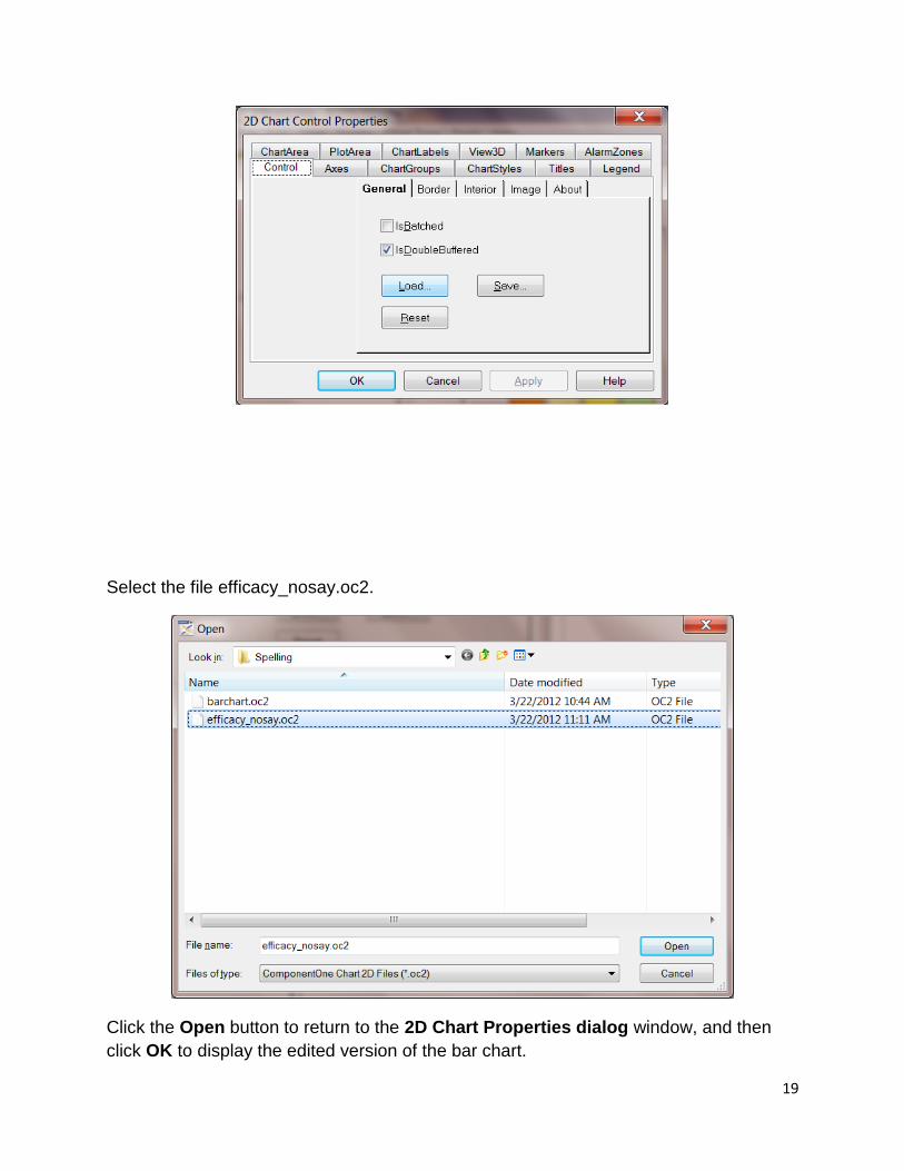
19

Select the file efficacy_nosay.oc2.

Click the Open button to return to the 2D Chart Properties dialog window, and then

click OK to display the edited version of the bar chart.

20

Is there an easy way to change the appearance of multiple graphs

The answer to this question is yes.

To illustrate, assume that a user wants to change the colors of the bar charts, displayed

when selecting the Graphics, Univariate… option using the dataset

AACL3_21Items.ssig (By DataSet\AACL folder).

Bar charts for the first 12 of the 21 Items are displayed below.

21

Right-click on the first graph to activate the 2D Chart Control Properties dialog. Then

select the ChartStyles, Style 1 option and choose CadetBlue to display the bar

associated with the first category as shown below.

22

Next select Style 2 and change the color to LightSalmon. These changes are shown

below for the item Afraid.

To replicate this (and any other changes), left-click on the first graph and select the

Copy Style option from the menu that is displayed as a result of this action, see below.

23

By left-clicking on each of the remaining 20 graphs, the Save, Load, Copy and Paste

style options are activated. Choose the Paste Style option to produce the same

appearance for each item. The result of these actions is shown for the first 11 items.

24

Saving and loading Styles

Once the appearance of a graph has been changed, one could save these changes in a

file with extension .csf. This is accomplished by left-clicking on the graph in question

and selecting the Save Style option. By doing so, a Save As dialog is displayed. In the

illustration below, the styles are saved in a file named AACL_21_Style.csf.

When the same .ssig file is opened and graphs are displayed, one can select the Load

Style option (by left-clicking on a graph) and browse for the saved style file. Once this

action is completed, use the Copy and Paste options described above to change any

one of the remaining graphs.

25

Can IRTPRO conduct an IRT analysis on repeated measures data?

Yes, for some situations and corresponding models IRTPRO can analyze data on repeated measurements or longitudinal data. See example 2.2 in Cai, L. (2010-a). A two-tier full-information item factor analysis model with applications. Psychometrika, 75, 581-612.

Does IRTPRO have the option of producing the estimated observed

scores based on the test characteristic curve?

When the test characteristic curve (see below) is plotted, it plots the "estimated observed score."

26

By clicking the Table button the underlying data being plotted is displayed as shown in the image below.

27

Does IRTPRO have the option of superimposing the empirical item

response curve to the estimated item response curve?

No. There are no "empirical item response curves" unless one uses point-estimates of the latent variable to create them. Historically, some have done that, but it's not endorsed here. IRTPRO _does_ provide the S-X2 statistics that are based on the difference between observed and expected frequencies in response categories by summed scores. If one selects the option to print the tables, one can see that information in tabular form, which is interpreted in much the same way as the nonexistent plots would be.

Can you provide more details on the tables on pages 76 to 78 and what

gray colors mean in the S-X2 tables?

On page 76 and 77 of the IRTPRO manual, there are two tables. In those tables there

are gray numbers in addition to the red and blue.

The gray numbers in the S-X2 tables; those are observed and expected frequencies in

cells that have expected frequencies less than 1.0 (or whatever the minimum value is

set to in Advance Options). The gray numbers have been "collapsed" into adjacent red

or blue numbers above or below them. For example, in the table on p. 76 of the User's

guide, the gray values 0, 0, and 1 total to the red "1" in the Score 6, Category 0 cell, and

the gray numbers 0.1, 0.6 and 2.1 add up to the red 2.8 that is expected in that

"collapsed" cell.

Remark

On page 77, the paragraph below the table says, "The printout below shows the

pairwise values of the standardized LD X2 statistics for this impulsivity subscale fitted

with the special model intermediate between the 1PL and 2PL models; italic entries

indicate positive LD, while roman entries indicate negative LD".

That paragraph mentions "italic" and "roman" in error; it was copied from a document

that was originally printed in black and white, so italic was used for positive LD and

roman for negative LD. In the actual output, for the LD X2 statistics, as it says on p. 96

of the User's Guide, "The values are printed in red if the observed covariation between

28

responses to a pair of items exceeds that predicted by the model, and in blue if the

observed covariation is less than fitted."

Therefore p. 77 should have "red" in place of "italic" and "blue" in place of "roman."

The "maroon" numbers on page 78 are a darker shade of red. There are also darker, as

well as brighter, blue numbers in that table.

The bright red and bright blue values are larger in absolute value than 3.0; the less

bright red and blue numbers have absolute values less than 3.0. The value of 3.0 is not

particularly meaningful; it merely serves as a very minimal arbitrary cut-off to make the

darker values less salient, because they almost certainly do not represent any important

LD.

There can be black numbers in those tables, if the nominal model is fitted and the item's

responses are not properly ordered.

Can IRTPRO compute standardized discrimination parameters?

IRTPRO has an option to print factor loadings (in the options-miscellaneous box), which

are standardized discrimination parameters.

How does one interpret the columns of the score file?

The columns of the score text output file are as follows (for K-factors):

Group Number (1, 2, 3...)

Case IDs (an internal id is always printed, and if the user selects an ID variable, it's also

printed)

K (number of dimensions) columns of score point estimates

K columns of SEs

K(K+1)/2 columns of the lower-triangular portion of the posterior covariance matrix (so

only the unique elements are printed as a list)

The last part is omitted for unidimensional IRT (K==1).