1

2

Table of Contents List of Tables ................................................................................................ Error! Bookmark not defined.

List of Figures........................................................................................................................................... 6

ACKNOWLEDGMENT .......................................................................................................................... 7

ABSTRACT.............................................................................................................................................. 8

INTRODUCTION .................................................................................................................................... 8

Irradiance Level at Ifrane ........................................................................................................................ 9

Solar Panels ............................................................................................................................................ 11

The photovoltaic Effect .......................................................................................................... 11

Types of Solar Panels ............................................................................................................. 11

The crystalline technology .................................................................................................. 11

The thin film technology ..................................................................................................... 12

Inverters ................................................................................................................................................. 13

String Inverters ....................................................................................................................... 14

Micro String Inverters............................................................................................................. 14

Centralized Inverters............................................................................................................... 15

Cables ..................................................................................................................................................... 17

Dimensioning .......................................................................................................................................... 17

Methodology .......................................................................................................................... 17

PV Modules Brand ................................................................................................................. 18

Inverter Brand ........................................................................................................................ 18

The Power Injected on the Grid .............................................................................................. 20

Losses ................................................................................................................................. 20

Dimensioning of the solar modules ......................................................................................... 22

Dimensioning of the inverter .................................................................................................. 22

Power compatibility ................................................................................................................ 22

Voltage Compatibility ............................................................................................................ 22

Current compatibility .............................................................................................................. 23

Junction Box........................................................................................................................... 24

CABLES Dimensioning ......................................................................................................... 24

Summary of the PV station .................................................................................................................... 26

Simulation PVsyst .................................................................................................................................. 27

Financial Analysis .................................................................................................................................. 32

Carbone footprint ................................................................................................................... 32

Production .............................................................................................................................. 33

3

Initial Investment .................................................................................................................... 33

Maintenance Cost ................................................................................................................... 34

Cash Flow Analysis ................................................................................................................ 35

Net Present Value (NPV) .................................................................................................... 35

Batteries .................................................................................................................................................. 38

Main Function ........................................................................................................................ 38

Type of batteries ..................................................................................................................... 38

A) Lithium ........................................................................................................................ 38

B) Lead .............................................................................................................................. 38

C) Nickel Cadmium ........................................................................................................... 39

Storage Principle .................................................................................................................................... 39

Battery Characteristics .......................................................................................................................... 40

Battery Basic Parameter ........................................................................................................................ 42

Voltage, Capacity and Energy ................................................................................................. 42

C-rate ..................................................................................................................................... 42

Storage Efficiency and Overall Battery Efficiency .................................................................. 43

SOC and DOD ........................................................................................................................ 43

Battery Cycles Life ................................................................................................................. 44

Battery Capacity and Temperature .......................................................................................... 45

Charging Controller ................................................................................................................ 45

Avoid Overcharging: Shunt CC .............................................................................................. 47

Dimensioning of the Battery .................................................................................................................. 47

Dimensioning of the charge controller .................................................................................... 48

Losses .................................................................................................................................... 49

Energy Stored & Delivered .................................................................................................................... 50

Financial Analysis for the Batterie System ........................................................................................... 51

Initial Investment .................................................................................................................... 51

Cash Flow Analysis ................................................................................................................ 52

STEEPLE Analysis ................................................................................................................................ 54

Conclusion .............................................................................................................................................. 55

List of Equations .................................................................................................................................... 55

References............................................................................................................................................... 56

Appendix ................................................................................................................................................ 58

Solar panels characteristics ..................................................................................................... 58

Inverter characteristics ............................................................................................................ 60

4

Battery characteristics ............................................................................................................. 61

Charge controller .................................................................................................................... 61

5

List of Tables Table 1: Comparison between the two types of technology and their solar cells .......................... 12

Table 2: Comparison between the 3 different topologies of Inverters .......................................... 16

Table 3:Ranking of Solar Companies in terms of Power Installation........................................... 18

Table 4: Comparison of different Inverters Rated Power ............................................................ 19

Table 5: Main Losses that the PV System Encounters ................................................................ 21

Table 6: Number of Panels in the System ................................................................................... 22

Table 7: Maximum Number of panels in series with an inverter ................................................. 23

Table 8: Annual Energy loss for cables ...................................................................................... 25

Table 9: Energy Loss Vs Cable length and Cross-sectional area ................................................. 25

Table 10: Monthly production of the Solar Plant ........................................................................ 30

Table 11: Carbon Footprint ........................................................................................................ 33

Table 12: Equipment Cost .......................................................................................................... 33

Table 13: Installation Cost.......................................................................................................... 34

Table 14: Other expenses ........................................................................................................... 34

Table 15: Summary Table .......................................................................................................... 36

Table 16: Cash flow over the year for the project 20MW............................................................ 37

Table 17: Comparison of the three types of batteries dominating the market............................... 39

Table 18: Characteristics of a Lithium Ion Smart Battery 12V/500Ah ........................................ 40

Table 19: Storage needed and new system efficiency ................................................................. 47

Table 20: Power delivered Vs Number of batteries Dimensioning .............................................. 51

Table 21: Initial batteries and charge controller investment ........................................................ 51

Table 22: Production cost of the system with batteries during the 5 months ................................ 52

Table 23: cash flow analysis of battery system ........................................................................... 53

6

List of Figures

Figure 1 Location of the site for weather and irradiance data on RET Screen............................................ 10

Figure 2: Solar Irradiance during the year at Ifrane ................................................................................... 10

Figure 3: Classic Solar Panel .................................................................................................................... 11

Figure 4Performance curves of a SMA 4000TL inverter .......................................................................... 13

Figure 5String Inverter Layout ................................................................................................................. 14

Figure 6 Micro String Inverter Layout ...................................................................................................... 14

Figure 7 Centralized Inverter Layout ........................................................................................................ 15

Figure 8: Process of Dimensioning ........................................................................................................... 18

Figure 9: Layout of the PV station ............................................................................................................ 24

Figure 10: Overview of a PV system ........................................................................................................ 27

Figure 11: Implementing weather Data of Ifrane in PVsyst....................................................................... 28

Figure 12: Orientation of the solar panels ................................................................................................. 28

Figure 13: Grid System Definition and Global Summary .......................................................................... 29

Figure 14: Adding Soiling and Snow loss parameters ............................................................................... 30

Figure 15: Second Page Result of the PVsyst simulation .......................................................................... 31

Figure 16: Losses Estimated by PVsyst .................................................................................................... 32

Figure 17: NPV Diagram for 25 years ...................................................................................................... 35

Figure 18: Grid Optimized Storage Using Lithium Ion Batteries .............................................................. 40

Figure 19: Layout of the solar plant with batteries .................................................................................... 40

Figure 20: Battery Capacity Vs Cycles ..................................................................................................... 44

Figure 21: Charge Controllers position in a PV system ............................................................................. 46

Figure 22: Maximum power point tracker in a charging controller............................................................ 46

Figure 23: Mechanism Shunt CC to prevent overcharging ........................................................................ 47

Figure 24: Design of the batteries ............................................................................................................. 48

Figure 25: SUNWAY SWD48V200 ......................................................................................................... 49

7

ACKNOWLEDGMENT

I thank from the bottom of my heart Dr. Khalid Loudiyi for given me the opportunity and the

moral support I need for this project. Solar power is an amazing field I would like to pursue my

studies on, and thanks to the advice, supervision and guidance he gave me throughout this

semester, I finally have the necessary knowledge to pursue my goal.

I thank Mr. Hamza El Hassnaoui, a chief project engineer from MASEN, who thaught me the

basic backgrounds behind a photovoltaic project and the use of the software PVsyst.

I would also like to thank Dr. Yassine Alj for directing this capstone and answer every ambiguous

questions I had.

Finally, I would like to thank my family and friends, who gave me the moral support I needed

throughout this whole semester.

8

ABSTRACT

This project is divided into two parts; the first one consists of analyzing the energy production of a

solar power plant of 20 MW based near the city of Ifrane. I will first make a correct dimensioning

of the PV station, making sure that the number of strings and inverters are well respected, and

finally calculating the energy production and the losses. Also, I will run a simulation using PVsyst

to match the results gathered before, and ending this part with a financial analysis.

The next part consists of including lithium ion batteries in order to store energy during the day and

release it at night during the periods of high solar intensity (May-September), we will need voltage

regulator that help protect the batteries from overcharging.

At the end, we need to determine if the two designs are complementary and beneficial for the city

of Ifrane on the long run. It should also be noted that both project will have separate financial

analysis in order to determine the profitability ration of each one.

INTRODUCTION

Since the Climate Change Conference that took place at Marrakesh in 2016, Morocco has been

financing huge amount of money towards renewable energy, and attracting foreign investors and

companies from all over the worlds like ACWA POWER, SENER or EDF. Just this year, the

Moroccan agency for solar energy has just financed 60 million euros for the project Noor Midelt

which will be composed of two technologies; CSP (Concentrated Solar Power) and Photovoltaic

panels. But this project is due to the huge success that other solar plants such as Ouarzazat,

Laayoune and Boujdour knew since their launch. There are currently eight solar plant in Morocco,

one is still under construction but the total energy provided until know is 680 MW. This is why I

strongly believe that solar plants are an excellent step forward for the future of Morocco, its

economy and environment. Morocco benefits of a solar radiation that is approximately 2200

9

KW/m²/year and 3000 hours of sunshine during the year, which makes the perfect conditions for

storing and producing solar energy. The Moroccan constitutional amendment n° 13 – 09

established on February the 11th 2010 has for objective to install a legal framework for any

individual or institution willing to invest or operate any type of facilities related strictly to

renewable energy. The amendment also includes a financial help plan, an environmental study, a

sustainable development plan that will promote job opportunities and proper infrastructure in the

region. It is highly recommended to run simulation using software like PVsyst to have an

approximation of the energy produced during the desired period, the size of the plant, the energy

loss due to the environment and many critical values that will determine the feasibility and

productivity of the project. The software also proposes oversize tools in case we want to increase

the production by adding more modules. It has mainly two functions, the first one is a pre-

dimensioning application easy to understand and configure.

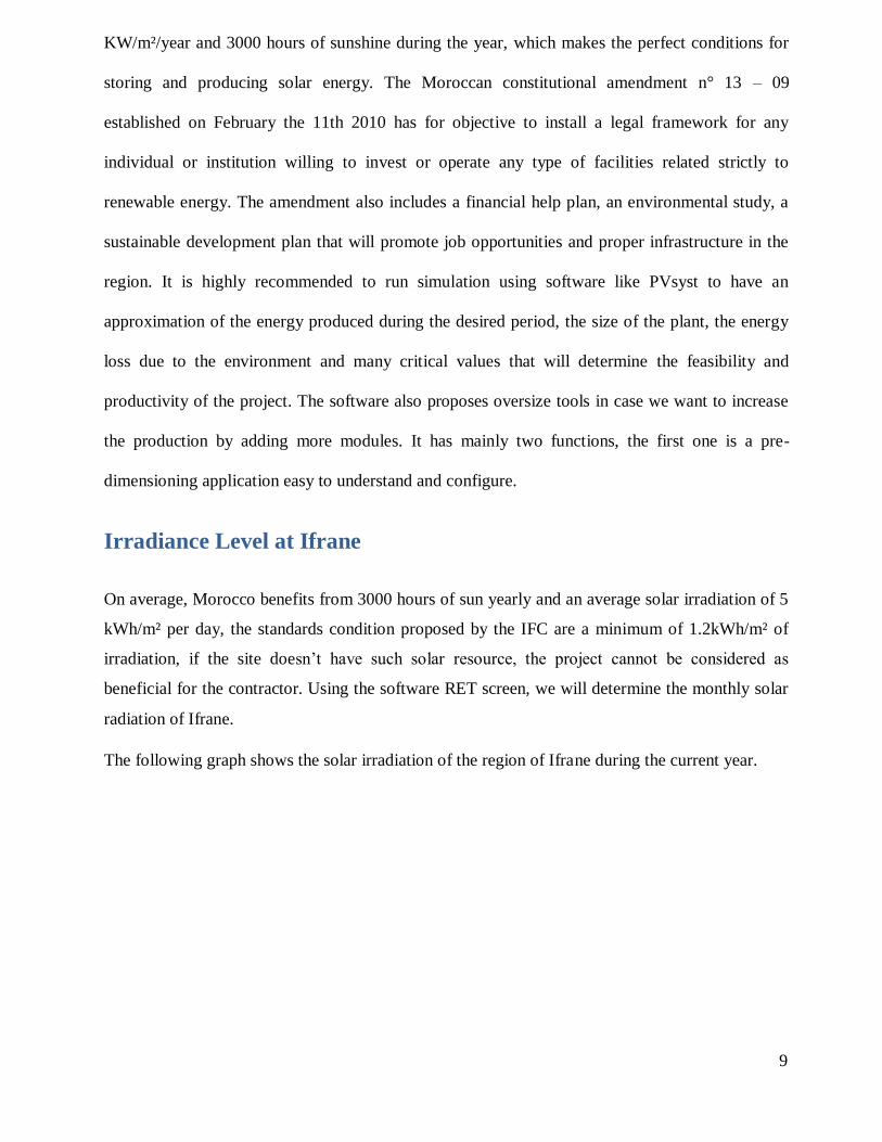
Irradiance Level at Ifrane

On average, Morocco benefits from 3000 hours of sun yearly and an average solar irradiation of 5

kWh/m² per day, the standards condition proposed by the IFC are a minimum of 1.2kWh/m² of

irradiation, if the site doesn’t have such solar resource, the project cannot be considered as

beneficial for the contractor. Using the software RET screen, we will determine the monthly solar

radiation of Ifrane.

The following graph shows the solar irradiation of the region of Ifrane during the current year.

10

.

Figure 1 Location of the site for weather and irradiance data on RET Screen

Figure 2: Solar Irradiance during the year at Ifrane

We clearly see that the region of Ifrane has a great potential regarding solar irradiation throughout

the year. The lowest: 2.92 kWh/m² per day during September and the highest goes to 8.97 5.92

kWh/m² per day in July.

11

Solar Panels

The photovoltaic Effect

The operation is as follows: the modules consist of two layers of semiconductor, a negative

charged layer and a positive charge layer based on silicon. These two layers of opposite signs

create an electric field. The light particles or photons strike the surface of the photovoltaic material

arranged in cells or thin layers and then transfer their energy to the electrons present in the

material which then move in a particular direction. The charges of opposite sign attract, and the

electrons will move to the positive layer from the negative charge. For example; if the upper layer

contains positively charged phosphorus atoms (with an electron deficiency) and the lower layer

contains negatively charged Bore atoms (with a surplus of electron), the applied heat will push its

electrons to move. This movement of charges generates an electric current, which is collected in a

conductive circuit placed under the cells and which connects all the cells of a panel.

Figure 3: Classic Solar Panel

Types of Solar Panels

The crystalline technology The crystalline technology uses thin and very thin cells, cut in an ingot obtained by melting and

molding silicon, then these cells are connected in series to each other to be covered by a protective

glass which will be composed of the module. There are three forms widely used in the

photovoltaic market, each differentiated by its performance, price and use condition:

Silicon Mono-cristallin

Silicon Poly-crystalline

Silicon Ribbon

12

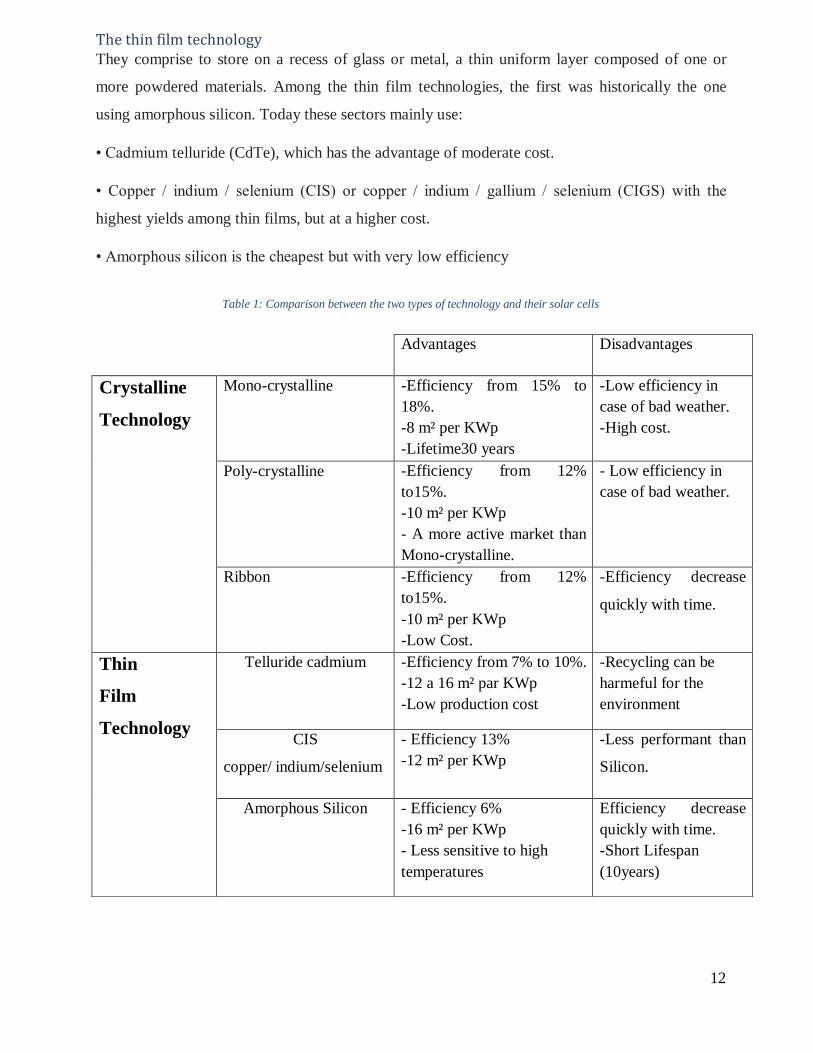
The thin film technology They comprise to store on a recess of glass or metal, a thin uniform layer composed of one or

more powdered materials. Among the thin film technologies, the first was historically the one

using amorphous silicon. Today these sectors mainly use:

• Cadmium telluride (CdTe), which has the advantage of moderate cost.

• Copper / indium / selenium (CIS) or copper / indium / gallium / selenium (CIGS) with the

highest yields among thin films, but at a higher cost.

• Amorphous silicon is the cheapest but with very low efficiency

Table 1: Comparison between the two types of technology and their solar cells

Advantages Disadvantages

Crystalline

Technology

Mono-crystalline -Efficiency from 15% to

18%.

-8 m² per KWp

-Lifetime30 years

-Low efficiency in

case of bad weather.

-High cost.

Poly-crystalline

-Efficiency from 12%

to15%.

-10 m² per KWp

- A more active market than

Mono-crystalline.

- Low efficiency in

case of bad weather.

Ribbon -Efficiency from 12%

to15%.

-10 m² per KWp

-Low Cost.

-Efficiency decrease

quickly with time.

Thin

Film

Technology

Telluride cadmium -Efficiency from 7% to 10%.

-12 a 16 m² par KWp

-Low production cost

-Recycling can be

harmeful for the

environment

CIS

copper/ indium/selenium

- Efficiency 13%

-12 m² per KWp

-Less performant than

Silicon.

Amorphous Silicon - Efficiency 6%

-16 m² per KWp

- Less sensitive to high

temperatures

Efficiency decrease

quickly with time.

-Short Lifespan

(10years)

13

It should be noted, however, that crystalline technologies are responsible for 96% of the global

production of photovoltaic modules. And that the polycrystalline market is the more relied on

since it offers approximately the same rate of production as the mono-crystalline over a long

period of time (Arno Smith, 2016).

Inverters Device for converting current and voltage, for example, from direct current to alternating current

or vice versa. Other names are used depending on the application: converter, rectifier, charger or

bidirectional inverter (D. Lalili, 2011).

The efficiency of an inverter reflects the power losses induced by its components. In fact, the

power delivered at the output AC is not equal (the power induced by the PV system) at the DC

input. The efficiency of an inverter is expressed by the following formula:

𝑃𝐴𝐶: Output power, 𝑃𝐷𝐶: Power delivered

𝑈𝑒𝑓𝑓,𝐴𝐶 , 𝐼𝑒𝑓𝑓,𝐴𝐶 : voltage / alternating current

cos 𝜑: power factor

𝑈𝐷𝐶 , 𝐼𝐴𝐶 : voltage / current delivered by the PV System

Figure 4Performance curves of a SMA 4000TL inverter

(1)

14

There are many types of inverter configuration, the most famous according to the SMA Academy

in their research paper “Inverter in large scale PV plants” are as following:

String Inverters

Micro String Inverters

Centralized Inverters

String Inverters In this architecture, an inverter is placed at the end of each chain, which aims to increase the

number of DC / DC converter, which leads to the possibility of extracting the maximum power.

This type of layout is generally less expensive and can be adapted in any kind of solar installation,

since there is only one inverter at each string.

Figure 5String Inverter Layout

Micro String Inverters This architecture uses a single inverter, while having a MPPT per string, using a chopper, which

reduces the number of interactions between the network and the PV system. The main interest is

to reduce the cost compared to the previous architecture, since the chopper does not need to

integrate functionalities of measurement and monitoring of the electrical data of the network.

Unfortunately, this system is expensive due to its constant maintenance, and regulations of each

microinverters.

Figure 6 Micro String Inverter Layout

15

Centralized Inverters A single inverter used converts total DC power into total AC power injected into the grid. This

architecture is:

Inexpensive

Easy to monitor

Simple and fast maintenance.

The mounting type of the figure has several defects:

- Solar conversion losses (only one MPPT for a set of modules).

- Electrical losses and risks in DC wiring.

- No continuity of service in case of failure of the inverter.

Figure 7 Centralized Inverter Layout

In the case of large photovoltaic installations, we have to choose one of the topologies. I will

conduct a comparative study based on these four criteria:

- Performance

- Yield

- Energy Quality

- Cost

The following table will help determine which topology is better for our solar plant:

L: low

M: Medium

16

H: High

V.H: Very High

Table 2: Comparison between the 3 different topologies of Inverters

central micro-string string

Reliability L M H

Performance

Strength H M L

Flexibility L

M

H

MPPT efficiency L M H

Mismatch H L H

Commutation H M H

Energy loss AC losses L M L

DC losses H

M

H

Variation tension AC L M L

Energy Variation tension DC V.H H M

Quality Tension Balance H L M

Installation Cost M M H

Cost

DC Cables H M L

C Cables H

M

M

Maintenance L H M

- Cost.

Note that the centralized topology has the following advantages: Robustness, low AC losses, low

AC voltage variation, and a reasonable cost of installation and maintenance compared to other

topologies. The general characteristics of the string and micro-string topologies are very attractive,

but the main disadvantages are the installation and the cost of maintenance, because the number of

inverters increases. For these reasons, I opted for the topology: centralized inverter.

17

Cables A cable is a perfect conductor in theory (Resistance = 0), but in practice it suffers losses of

current. Due to heating, there is a voltage drop and therefore a dissipation of energy expressed in

joule. It is necessary to minimize the loss of energy so that the photovoltaic plant has a better

profitability. It is therefore preferable to make a field visit for the dimensioning, because the loss

is mainly related to the length of the cables.

The sizing of cables within a PV installation is based on two fundamental points:

1. The use of unipolar double insulated cables in order to withstand the external conditions.

2. Sizing of a sufficient section so that the overall voltage drop is at most 3% and ideally 1%.

For this we will use copper-based cables: EXZHELLENT SOLAR ZZ-F - 0,6/1 kV (ρ = 1.6 10-8

Ω.m) according to the norm proposed by UTE C 32-502 for PV installation. The cables are known

to have a very low resistance and a voltage drop of 3% to 2%. A proper dimensioning of the cable

will be done in the part “Dimensioning”

Dimensioning

Methodology The solar plant consists of several sub-fields, each sub-field consists of blocks of photovoltaic

panels. In this part I will size the photovoltaic plant, choosing the modules, the inverter, and the

dimensioning of the cables (for the size of the park, refer to the UTE guide C15-712-1). While

respecting the requirements of the standard, and following the methodology expressed in Figure 6,

this calculation method is based on the classical design relationships of PV installations from the

arrival of the radiation to the panels until the injection to the network.

This method is preferable and more reliable since it is flexible in terms of choice of assumptions.

I will detail the calculations as well as the relationships used in each step of my work.

18

Figure 8: Process of Dimensioning

PV Modules Brand I choose the company “Jinkosolar” because of its impact on the solar market. Indeed, the company

was ranked 3rd in 2015 in terms of solar installation, and has since then been dominating the solar

sector. Another reason why I choose this company; it’s because almost all their solar panels are

available in PVsyst especially the Polycrystalline type that is best fitted for the region of Ifrane.

Table 3:Ranking of Solar Companies in terms of Power Installation

Thus, I decided to go for a module of 310 Wp Polycrystalline from Jinkosolar.

Inverter Brand

As stated previously in the “Inverter part”, I will go for a centralized inverter system. Now, I need

to determine a good inverter brand that I will incorporate in the system. The most appropriate

1

•Choose the PV module

•Choose the inverter

2

•Determine the Installation Power

3

•Dimensioning of the Solar Modules

4

•Dimensioning of the inverters

5

•Dimensioning cables

19

scenario is the Ingecon solution, as it is the most technically optimized with maximum energy

exploitation, few supply constraints and less components.

I finally opted for a centralized inverter configuration and an Ingecon inverter. What I will do is to

divide our 20 MW plant to mini plants for the centralized inverters, so in this paragraph we will

proceed with a technical and economic study to establish the best configuration of mini plants in

order to determine what is the optimal power for each mini power plant, in other words; what will

be the power of the optimal inverter from a point of view economic and technical, and of course

what would be the configuration that will allow us to produce more energy, that is to say generate

the most income.

For this, we used simulations with the PVsyst software to see the annual production of each

configuration and also a price search at the supplier and manufacturer level (Prinso store) to make

the optimal choice for our plant.

The methodology is simple, we will simulate every inverter accordingly to their power rating with

the solar panels that we choose (Jinkolsar 310 Wp polycrystalline) in order to compare how many

inverters we need, how much it will produce, its performance ratio and the total price that will be

invested .

Table 4: Comparison of different Inverters Rated Power

Panel Inverter Number of inverters Production(MWh) Pr(%) Total Price (MAD)

310 Wp

100 kW 61 11 308 MWh/year 80.4 56 400 000.00

250 kW 28 12 962 MWh/year 81.3 51 599 400.00

500 kW 17 15 860 MWh/year 82.0 45 960 000.00

1000 kW 10 17 815 MWh/year 82.4 37 214 236.00

We can clearly determine from table that the annual production of the inverters increases with the

power rate, likewise for the index of performance that exceeds 80%, which proves that our

photovoltaic installation works efficiently. Also, it can be noticed that the initial investment cost

of 1 MW inverters is lower than the others.

It can be concluded that for the rest of this study I will opt for an inverter of "Ingecon" with a

power of 1MW.

20

The Power Injected on the Grid

In order to determine the power delivered by the station, it’s highly recommended to anticipate the

losses that the solar plant will encounter during its operation. The losses can be determined from

the arrival of the solar irradiation to the cables injecting the current into the grid.

Losses

The solar panels have four main element that are affecting their performance; mismatch losses,

quality of the modules, temperature losses, and irradiance.

Mismatch Losses

According to ‘PV EDUCATION’ Mismatch losses are due to the interconnection of the solar cells

which have different status of functioning at the delivery of the power, for example; if a zone in

the panel is shaded or experience a different change in temperature than the other, it can affect the

power output delivered by the entire panels. Generally, the losses are between 0.5% and 1%

(Thomas S., Markus B. Schubert, 2014), the PVsyst software take the worst case which is 1% in

its analysis for losses.

Quality of the modules

It’s considered to be the module performance and act as a positive loss at standard condition, for

the model JKM 310PP-72 the quality loss is approximately 0.7%.

Temperature Probably the heaviest loss incurred during the functioning of the panels, it can be estimated using

the following equation:

𝑈 = 𝛼 × 𝐼𝑟𝑟 × (1 − ɳ)

(𝑇𝑐𝑒𝑙𝑙 − 𝑇𝐴)

𝑈: Factor of temperature losses

𝛼: Absorption coefficient (0.9)

𝐼𝑟𝑟: Irradiation on the solar panel

ɳ: Efficiency of the solar panel

𝑇𝑐𝑒𝑙𝑙: Temperature at the solar cells

𝑇𝐴: Ambient temperature

Irradiance Low-light efficiency, it depends on the PV module parameters Rserie and Rshunt (0.1%)

according to standard conditions proposed by PVsyst.

(2)

21

Cables losses The cable losses are estimated in the worst cases to not exceeds 3% of the losses, this figure can

be determined while doing the dimensioning of both AC and DC cables. I will go into more details

regarding the cables losses in the dimensioning part of both AC and DC. It should be noted that

PVsyst proposed the norm loss of 3% by default when it’s simulating.

Inverter losses The Ingecon Sun 1000TL U X400 has an efficiency conversion of 98.52% which mean a loss of

1.48%, knowing that there might be some other variables that cannot be determined while

computing the loss of an inverter, I’ll take this variable to be 2%.

Total losses There are also other independent variables that affect the losses like soiling, snow, the change of

radiation during the day (Didier T., Sophie P., 2011).

Table 5: Main Losses that the PV System Encounters

Missmatch -1%

Quality of the Module +7%

Temperature -10.3%

Irradiance +0.1%

Cables -3%

Soiling and Dirt -2%

Snow -1.5%

Inverter -2%

DistributionTransformer THT -2%

Finally, the power injected can be determined by the following formula (Masters, 2004):

𝑃𝑖𝑛𝑗 = 𝑃𝑛 × ∏ 𝐿𝑇

→ 𝑃𝑖𝑛𝑗 = 20𝑀𝑊 × (0.99 × 1.07 × 0.897 × 0.99 × 0.97 × 0.98 × 1.001 × 0.985 × 0.98)

𝑃𝑖𝑛𝑗 = 17.20 𝑀𝑊

𝑃𝑖𝑛𝑗: Power injected in the grid

𝑃𝑛: Nominal Power of the station

∏ 𝐿𝑇: Product of the main losses

(3)

22

Dimensioning of the solar modules In this part, I’ll start by determining the maximum number of panels needed, the following

formulas will help us calculate the number of panels according to the power needed for the station

and the power capacity of the modules; it’s the integer of the nominal power of the station divided

by the power of one solar panel.

𝑁 = [𝑃𝑛

𝑃𝑆𝑀]

→ 𝑁 = [20𝑀𝑊

310 𝑊]= 64 517 panels

𝑃𝑛: Nominal Power of the station

𝑃𝑆𝑀: Power peak of each module

Table 6: Number of Panels in the System

Nominal Power of the Station Panel power Maximum Number of panels

20MW 310Wp 64 517

Dimensioning of the inverter After the calculation of the numbers of panels, we proceed to the dimensioning of the inverters,

this step aims at the computation of the modules in string and in series for each inverter, but the

number of inverters rests on 3 criteria:

Power compatibility, voltage compatibility and current compatibility.

From these 3 criteria, the dimensioning of the inverters will impose how to wire the modules

together.

Power compatibility An inverter is characterized by a permissible power input, so make sure that the calculated power

remains within the permissible power range of the inverter shown in the data sheet. For our case

the power margin at the input of each inverter is between 1120 and 1627 KWp. By dividing the

power of the field by the number of inverters, we find:

20𝑀𝑊

15= 1 333 𝐾𝑊𝑝 → 1120|1627

Voltage Compatibility An inverter is characterized by a maximum permissible input voltage Umax. If the voltage

delivered by the PV modules is greater than Umax, the inverter will be irreparably destroyed.

In addition, since the voltage of the PV modules is added when connected in series, the value of

Umax will therefore determine the maximum number of modules in series.

In the dimensioning, it is considered that the voltage delivered by a module is its no-load voltage,

noted Uco, increased by a safety factor (or correction), denoted Ku

So according to the formula

(4)

(5)

(6)

23

𝑀𝑎𝑥𝑖𝑚𝑢𝑚 𝑁𝑢𝑚𝑏𝑒𝑟 𝑜𝑓 𝑀𝑜𝑑𝑢𝑙𝑒𝑠 𝑖𝑛 𝑆𝑒𝑟𝑖𝑒𝑠 = [𝑈𝑚𝑎𝑥

𝑈𝑐𝑜×𝐾𝑢]:

𝑈𝑚𝑎𝑥 : Maximum voltage allowed at the entry of the inverter

𝑈𝑐𝑜: PV module voltage when the circuit is open

𝐾𝑢: Safety factor denoted by: 1 + (αUoc / 100) x (Tmin – 25)

αUoc: coefficient of variation of the module voltage in temperature, in % / ° C

Tmin: Minimum ambient temperature (-10°C for Ifrane)

Table 7: Maximum Number of panels in series with an inverter

𝑈𝑚𝑎𝑥 𝑈𝑐𝑜 𝐾𝑢 Panels in Series

1000V 49.5V 1.091 19

Current compatibility An inverter is characterized by a maximum permissible input current. This limit input current

corresponds to the maximum current that can be withstood by the DC side inverter. When the

input current is greater than this current, the inverter continues to operate, but provides the

network with the power corresponding to its maximum current. Therefore, I must be careful to

ensure that the current delivered by the PV array does not exceed the value of the maximum

permissible current Imax by the inverter. Moreover, since the currents are added when the chains

are in parallel, the value of Imax will determine the maximum number of photovoltaic chains in

parallel. This will obviously depend on the current delivered by a photovoltaic chain. In the

design, it will be considered that the current delivered by the string is equal to the maximum

power current Impp of the photovoltaic modules.

𝑀𝑎𝑥𝑖𝑚𝑢𝑚 𝑁𝑢𝑚𝑏𝑒𝑟 𝑜𝑓 𝑃𝑎𝑛𝑒𝑙𝑠 𝑖𝑛 𝑝𝑎𝑟𝑎𝑙𝑙𝑒𝑙: [𝐼𝑚𝑎𝑥

𝐼𝑚𝑝𝑝]

[1730

8.38] = 206

For the inverter chosen, it has 16 inputs with a maximum current that can withstand the inverter of

1730 A. For our case we will use 13 inputs with a maximum current for each input of 108.12 A

Hence the maximum number of string per inverter is: 𝑁𝑠𝑡𝑟𝑖𝑛𝑔 = 15 × 13 = 195

Previously we determined that the number of panels in series should not exceeds 19, Therefore;

The number of panels per inverter = 195 × 19 = 3 705 𝑝𝑎𝑛𝑛𝑒𝑙𝑠 𝑝𝑒𝑟 𝑖𝑛𝑣𝑒𝑟𝑡𝑒𝑟.

And finally: The power injected in each inverter is = 310 Wp × 3 705 = 1 148.5 kWp

(7)

24

Junction Box The use of 13 input of the inverter means the use of 13 junction box, for each junction box we will

use Y connectors to group two parallel string.

The following figure is a template from Noor Boujdor, for each junction box we will use 15 string

ie 8 Ve + connectors and 8 Ve- connectors.

Figure 9: Layout of the PV station

CABLES Dimensioning According to a study done by Sami Ekici and Mehmet Ali Kopru published by the International

Journal of Renewable Energy Research (Investigation of PV System Cable Losses, 2017), the

cable length or cross-sectional area does not affect significantly the performance of the solar pv

system, and can be disregarded, however; as stated previously, they took into consideration the

current Iz and the voltage drop, adding the resistivity of the cable.

Moreover, it should be noted that the resistivity of a material can be highly influenced by its cross-

sectional area. Here is a table of energy loss according to the cross-sectional area:

25

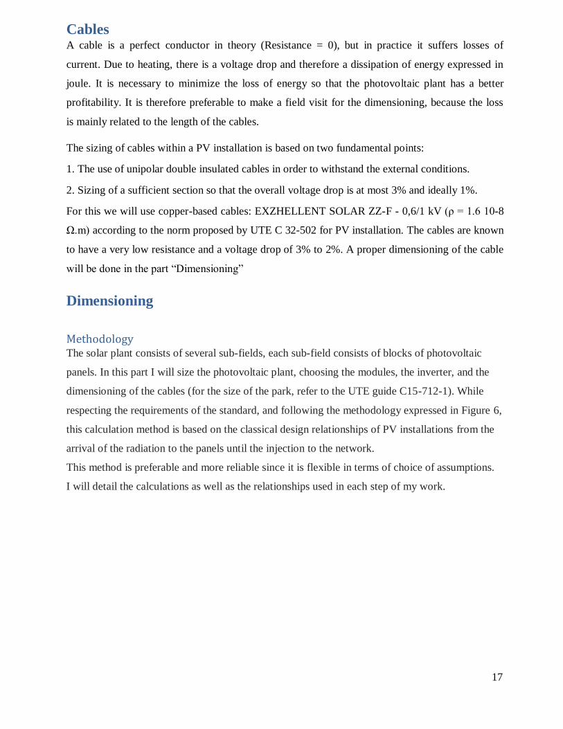
Table 8: Annual Energy loss for cables

OHM

LOSS

Cross Sectional Area Annual Energy loss (kWh)

1.5 mm² 2.795

4.0 mm² 1.048

10 mm² 0.419

Therefore, it can be concluded that the bigger the cross-sectional area of the cable, the smaller the

losses. Using PVsyst “wiring layout”, the following figure shows how the energy loss change with

respect to the cross-sectional area and the length of the cable.

Table 9: Energy Loss Vs Cable length and Cross-sectional area

According to (Sami E. & Mehmet A. 2017) and (Michael M.D. Ross 2005) the formula for wiring

losses is: 𝑃𝑙𝑜𝑠𝑠 = 2 × 𝐼𝐷𝐶2 × = 2 × (

𝑃𝐷𝐶

𝑉𝐷𝐶)² ×

𝑃𝑙𝑜𝑠𝑠: Cable loss, DC resistance, 𝑃𝐷𝐶: Power available in the DC cables

𝐼𝐷𝐶2 : DC current, 𝑉𝐷𝐶 : DC voltage.

26

We are using a cable made of copper which has a resistivity of 1.6 × 10−8Ω.

The DC current is just the power of the panels divided by the DC voltage in the string

connected to the inverter: 𝐼𝐷𝐶 =𝑃𝐷𝐶

𝑉𝐷𝐶=

310

49.5 = 6.26 A.

Therefore 𝑃𝑙𝑜𝑠𝑠 = 2 × (6.26)2 × 1.6 × 10−8 = 1.25 × 10−6 for one string

There are 195 strings in each inverter → 𝑃𝑙𝑜𝑠𝑠 = 2.6 × 10−4

There are 15 inverters in the station → 𝑃𝑙𝑜𝑠𝑠 = 3.9 × 10−3 < 3%

The string length can be determined 𝐿𝑠𝑡𝑟𝑖𝑛𝑔 = 19 𝑚𝑜𝑑𝑢𝑙𝑒𝑠 +

2𝑚 (𝑑𝑖𝑠𝑡𝑎𝑛𝑐𝑒 𝑡𝑜 𝑖𝑛𝑣𝑒𝑟𝑡𝑒𝑟)

Cross-sectional area can be determined by the following equation:

𝑆 = × 𝐿 × 𝐼

𝑃𝑙𝑜𝑠𝑠 × 𝑈

: Resistivity of the cable 1.6 × 10−8Ω

𝐿: Length of the cable

𝐼: current of the parallel modules

𝑃𝑙𝑜𝑠𝑠: The losses incurred in the cables

𝑈: Voltage across the modules in series

𝑆 = 1.6 × 10−8 × 34 × 208 × 6.26

3.9 × 10−3 × 19 × 49.5= 355 𝑚𝑚²

According to this result I should pick a solar cable of 1x400 mm² available at EXZHELLENT

SOLAR ZZ-F, the total length of the cables couldn’t be determined since it needs a complete

and detailed dimensioning of the PV station with other components like a control room,

lightning protection system, fences, ect….

Summary of the PV station So far, I determined the number of solar modules, the number of string, inverters and respect the

norm in which they will function at full efficiency while making the necessary calculations to

avoid overheating or unnecessary damages especially regarding the inverter. Here are the

specifications of the PV station:

Nominal Power of the Station: 20 MW

Panel Jinkosolar: JKM 310PP-72

Total Numbers of modules : 64 517 – 55 575

Inverter Ingeteam: Ingecon Sun 1000TL U X400 Outdoor 1MW

Number of Inverter: 15

(8)

27

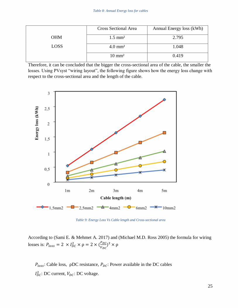
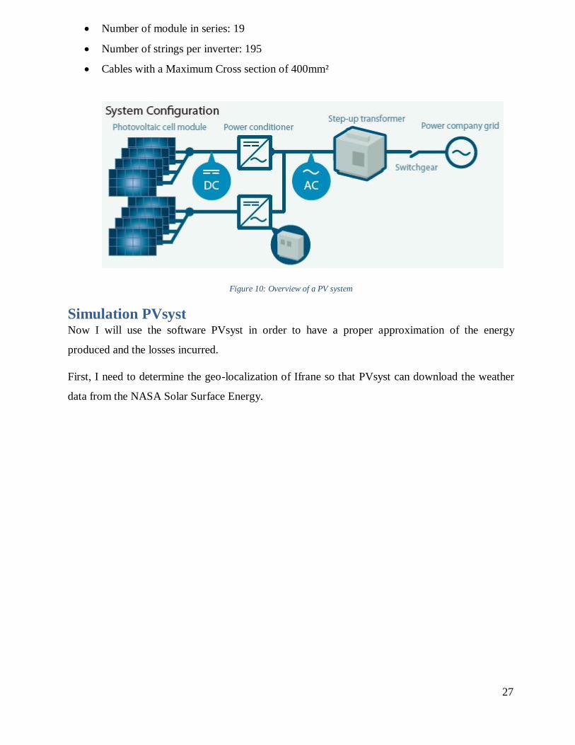
Number of module in series: 19

Number of strings per inverter: 195

Cables with a Maximum Cross section of 400mm²

Figure 10: Overview of a PV system

Simulation PVsyst Now I will use the software PVsyst in order to have a proper approximation of the energy

produced and the losses incurred.

First, I need to determine the geo-localization of Ifrane so that PVsyst can download the weather

data from the NASA Solar Surface Energy.

28

Figure 11: Implementing weather Data of Ifrane in PVsyst

Once our site is recognized by the software, and the weather and irradiation data included we can

move to the second step, which is defining what type of system we want to use. Since we are

injecting directly into the local grid, it’s a Grid-connected system. I’ll need to define 3 mandatory

inputs before simulating our PV plant.

There is first the tilt angle, according to the installation near the AUI gymnasium, the panels are

facing south with an angle of 32° and an Azimuth of 0.

Figure 12: Orientation of the solar panels

29

Then we have the most important input out of the three; the global system configuration. I’ll start

first by entering the initial specifications, either the available area or the nominal power of the

solar plant. I’ll enter the 20MW needed and it will automatically generate a minimum surface area

and an approximate number of panels depending on the model used.

After that, we select the solar module that we want (JKM 310PP-72) and the inverter (Ingecon

Sun 1000TL U X400 Outdoor). We determine the number of inverter, in our case 15, and design

the array.

Now this part is a little bit tricky since we need to determine the number of strings and module in

series, the dimensions impact on the voltage and current injected in the inverter should not exceed

the operating conditions. At the same time, we need to push for a maximum number of strings and

modules in order to get a higher energy production.

Figure 13: Grid System Definition and Global Summary

The final step before simulating is adding some losses that PVsyst didn’t take care into

consideration like soiling and snow. As stated previously when I talked about losses, soiling and

snow are defined to be approximatively 2% and 1.5% (Didier T., Sophie P., 2011). So, we go to

the detailed loss parameter and add the 3.5% loss of soiling and snow effect.

30

Figure 14: Adding Soiling and Snow loss parameters

Now we can move to the simulation, the software proceed by giving us three pages of detailed

results. The first page shows all the major parameter entered, like the type of module and inverter,

their nominal power and number.

The second page is more interesting since it gives us the energy production during the year, the

irradiation at every month and the energy injected into the grid system.

Table 10: Monthly production of the Solar Plant

31

Figure 15: Second Page Result of the PVsyst simulation

The last page show the losses in the irradiation, the losses of the electrical energy in the cables that

connect the solar panels, the losses due to the elevation of the temperature of the PV plant, the losses

due to the quality of the PV panels as well as losses at the inverter level.

32

Figure 16: Losses Estimated by PVsyst

Financial Analysis

Carbone footprint The carbon footprint makes it possible to estimate the impact of this installation on the

environment. This balance is calculated on the basis of emission factors that vary according to the

type of energy used. The emission factor for photovoltaic installations, according to a recent study

by the French agency ADEMEE (Agency for the Environment and Energy Management), is equal

33

to 55 geqCO2 for each kWh produced, whereas the quantity of CO2 released to generate a kWh

using fossil fuels and average of 728 g.

Table 10 shows the different emissions as well as the carbon return time. The latter represents the

time required for a photovoltaic installation, by substituting electricity produced by conventional

energies, to avoid the emissions that were necessary for its manufacture, installation and

maintenance. The formula used to calculate the carbon time is represented by the following

equation:

𝐶𝑎𝑟𝑏𝑜𝑛 𝑅𝑒𝑡𝑢𝑟𝑛 𝑇𝑖𝑚𝑒 (𝑦𝑒𝑎𝑟)

=𝐸𝑚𝑖𝑠𝑠𝑖𝑜𝑛 𝑜𝑓 𝑡ℎ𝑒 𝑃𝑉 𝑖𝑛𝑠𝑡𝑎𝑙𝑙𝑎𝑡𝑖𝑜𝑛 𝑑𝑢𝑟𝑖𝑛𝑔 𝑖𝑡𝑠 𝑙𝑖𝑓𝑒𝑡𝑖𝑚𝑒

𝑒𝑚𝑖𝑠𝑠𝑖𝑜𝑛 𝑑𝑢𝑒 𝑡𝑜 𝑡ℎ𝑒 𝑎𝑛𝑛𝑢𝑎𝑙 𝑐𝑜𝑛𝑠𝑢𝑚𝑝𝑡𝑖𝑜𝑛 𝑜𝑓 𝑡ℎ𝑒 𝑙𝑜𝑐𝑎𝑙 𝑛𝑒𝑡𝑤𝑜𝑟𝑘

Table 11: Carbon Footprint

Production

GWh/year

Emission of 1Kw

of PV (eq CO2)

Emission of the

PV plant

(lifetime)

Annual emission

for fossil

energies

Carbon Return

Time

30 55 5.5 × 1010 2.91× 1010 1.89 year

Emissions related to this facility are amortized in less than 2 years. Thus, throughout the rest of its

estimated life of 25 years, the operation operates with zero emissions and avoids annually 2.91 ×

1010g of CO2.

Production In order to evaluate the profitability of the PV installation, it is first necessary to calculate the 25-

year average production cost of 30 169 MWh if the energy is supplied by the ONEE. Knowing

that the price per kWh is 1.36 MAD, the annual cost is therefore 41 029 840.63 MAD / year for 25

years.

Initial Investment The following table presents the cost of the different equipment needed for the station:

Table 12: Equipment Cost

Equipment Cost per unit

(MAD)

Number of Unit Total Cost (MAD)

Solar Panel 2509,93 55 024 138 106 388,3

Inverter 2 480 949 15 37 214 235

34

Cables (400mm²) 16 for 1m 83737,575* 1 339 801,2

Junction Box 120 195 23 400

BT/HTA Transformer 2 200 000 7 15 400 000

Network Connection 0.5 17 057 000 8 528 500

HTA/HT Transformer 35 000 000 1 35 000 000

Auxiliary Transformer 4 000 000 1 4 000 000

Central CB circuit

breaker**

3 000 000 1 3 000 000

Total Price 207 612 324,50

*: Those dimensions were taken from Noor Boujdor which has a capacity of 15MW

**: It should also be noted that we didn’t take into consideration other prices like the protection

system or anti-lightning devices

Installation costs are calculated at 180 MAD / m² and transport costs are 10% of the cost of the

installation work, the feasibility study is 2% of the initial investment, and finally; unexpected

expenses that should be 10% of the initial cost.

Table 13: Installation Cost

Element Unit Quantity Price (MAD) Total Price(MAD)

Installation cost m² 96 413 180 17 354 340

Transport … … … 1 735 434

Table 14: Other expenses

The feasibility study (2%) 4 152 246.49 MAD

Unexpected Expenses (10%) 20 761 232.45 MAD

The total initial cost for the first year of production is then: 251 615 576.5 MAD

Maintenance Cost If the photovoltaic technology is deemed reliable and without heavy maintenance, slight

maintenance operations are still necessary to prevent any problems and ensure that the safety

devices are working. The frequency of the interventions listed depends in part on the quality of the

site (pollution, dust ...). In most cases, an annual visit with the operations listed below is sufficient

as a routine check:

Visual inspection of the modules;

35

The cleaning of the modules;

Snow removal of the modules;

Verification and dedusting of the inverters;

Inspection of DC boxes;

Signage;

Recorded intervention report.

In this project, the maintenance cost is estimated at 5% of the initial investment. As a result, the

maintenance costs amount to 10 380 616.23 MAD/year.

Cash Flow Analysis The financial analysis of a photovoltaic project is needed to evaluate the profitability and the price

of the KWh produced by the installation. In this part we will determine the net present value that

will help us estimate the accumulated cash flow. Finally, we will determine the performance index

which will give us when the project will give a return on investment.

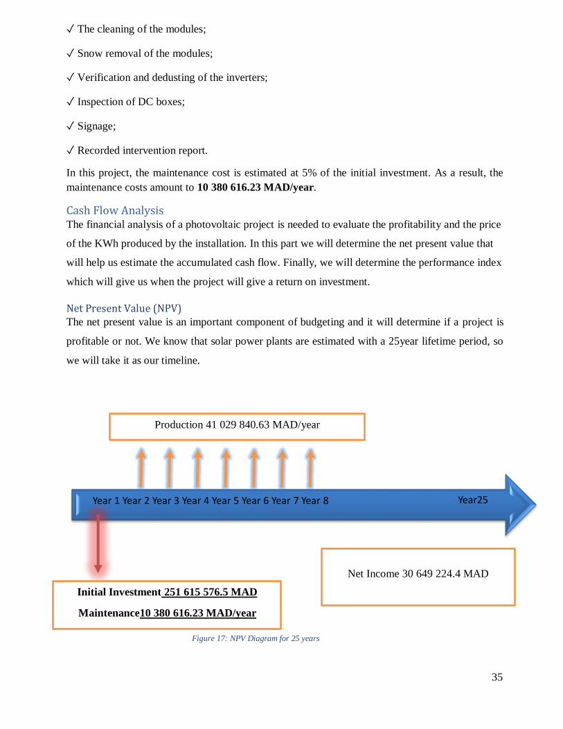
Net Present Value (NPV) The net present value is an important component of budgeting and it will determine if a project is

profitable or not. We know that solar power plants are estimated with a 25year lifetime period, so

we will take it as our timeline.

Year25Year 1 Year 2 Year 3 Year 4 Year 5 Year 6 Year 7 Year 8

Initial Investment 251 615 576.5 MAD

Maintenance10 380 616.23 MAD/year

Production 41 029 840.63 MAD/year

Net Income 30 649 224.4 MAD

Figure 17: NPV Diagram for 25 years

36

The NPV formula is defined as the initial investment plus the present value of the cash received at

a specific year;

𝑁𝑃𝑉 = −𝐼𝑛𝑖𝑡𝑖𝑎𝑙 𝑖𝑛𝑣𝑒𝑠𝑡𝑚𝑒𝑛𝑡 +𝐶𝑎𝑠ℎ 𝑎𝑡 𝑦𝑒𝑎𝑟 𝑡

(1 + 𝑟)𝑡

Where 𝑟 is the inflation rate, it stands at 1.3% in Morocco for the year 2016.

Then we have the cumulative cash flow for a given year. It is the sum of discounted cash flows of

the year plus previous years:

And finally, the profitability index; IP. It is the ratio between the sum of discounted cash flows

and the initial investment amount. A project is profitable if its IP is greater than 1.

Before we proceed to the calculations, here is a summary table of the data gathered that we will

work with.

Table 15: Summary Table

Initial Investment 251 615 576.5 MAD

Production 41 029 840.63 MAD/year

Maintenance 10 380 616.23 MAD/year

Lifetime 25 years

Net Income 30 649 224.4 MAD

Inflation Rate 1.3%

Once we have every information needed, we can draw a table containing the evolution on the NPV

thought the year, the accumulated cash flow and the performance index.

(9)

(10)

(11)

37

Table 16: Cash flow over the year for the project 20MW

Year Net Income Accumulated

Cash flow NPV

Profitability

Index

1 30 649 224,40 30 649 224,40 - 224 492 369,07 0,12

2 30 373 381,38 61 022 605,78 - 194 118 987,69 0,24

3 30 100 020,95 91 122 626,73 - 164 018 966,74 0,36

4 29 829 120,76 120 951 747,49 - 134 189 845,98 0,48

5 29 560 658,67 150 512 406,16 - 104 629 187,31 0,60

6 29 294 612,74 179 807 018,90 - 75 334 574,56 0,71

7 29 030 961,23 208 837 980,13 - 46 303 613,33 0,83

8 28 769 682,58 237 607 662,71 - 17 533 930,75 0,94

9 28 510 755,44 266 118 418,15 10 976 824,68 1,06

10 28 254 158,64 294 372 576,79 39 230 983,32 1,17

11 27 999 871,21 322 372 447,99 67 230 854,53 1,28

12 27 747 872,37 350 120 320,36 94 978 726,90 1,39

13 27 498 141,52 377 618 461,88 122 476 868,41 1,50

14 27 250 658,24 404 869 120,12 149 727 526,66 1,61

15 27 005 402,32 431 874 522,44 176 732 928,98 1,72

16 26 762 353,70 458 636 876,14 203 495 282,67 1,82

17 26 521 492,51 485 158 368,65 230 016 775,19 1,93

18 26 282 799,08 511 441 167,74 256 299 574,27 2,03

19 26 046 253,89 537 487 421,63 282 345 828,16 2,14

20 25 811 837,61 563 299 259,23 308 157 665,77 2,24

21 25 579 531,07 588 878 790,30 333 737 196,83 2,34

22 25 349 315,29 614 228 105,59 359 086 512,12 2,44

23 25 121 171,45 639 349 277,04 384 207 683,57 2,54

24 24 895 080,91 664 244 357,94 409 102 764,48 2,64

25 24 671 025,18 688 915 383,12 433 773 789,65 2,74

The table show that the installation will start making profit after 8 years of functioning, given the

fact that it is very difficult to predict the weather in the years to come, it appears that it will be

very difficult for the designer and even for a simulation software to estimate exactly the annual

production of a PV installation, which will give a gain relatively different from the one estimated.

However, a solar power station in most cases is profitable in the relatively near future when a

rigorous accounting of the external costs of the various components of production will be

conducted. In this part we presented an economic analysis of our photovoltaic system taking into

account the relative cost of the components of the production system. This study has finally

38

resulted in an estimate that can generate a gain of 433 773 789, 65 DH over 25 years, with a return

on investment of 8 years.

Batteries

Main Function The primary role of the battery is to store during the day the necessary energy during the night; its

minimum capacity to satisfy this function can be calculated simply; secondly, it must serve as a

security buffer during the periods of several consecutive days without sun; finally, it must fill

during the summer the winter deficit.

Type of batteries

A) Lithium For lithium battery technology, many variants exist with different electrolytes and combinations

of electrodes, each leading to different properties, such as lifetime or safety. This can generate

significant development potential, and therefore, cost reduction.

B) Lead

i. - Solar battery with open lead

This battery has a long service life of more than 10 years, contains good resistance to extreme

temperatures (inertia of the liquid electrolyte), and a tryearsparent tank to visualize the acid level

and the state of battery. The open lead-to-tube battery is robust, but requires regular maintenance.

At low load it gives an estimate of 400 to 500 cycles.

ii. - Solar battery AGM

The AGM waterproof battery is a compromise between the open lead battery and the gel

battery. It is often used for engine start-ups. Unlike an open lead battery, it requires no

maintenance, has a very good resistance to shocks and vibrations and a very low release of

hydrogen (explosive). In low load it gives an estimate of 600 to 700 cycles.

iii. - Solar battery GEL

The sealed battery with gelled electrolyte is the "high end" of the lead batteries and does not

require maintenance. It can withstand shocks and vibrations and has a lifetime of 5 to 15 years.

The battery can withstand extreme temperatures (-20 / + 55 ° C) and does not trigger electrolyte

lamination (no leakage of electrolyte). At low load it gives an estimate of 800 to 900 cycles

39

C) Nickel Cadmium

A Nickel-Cadmium or Ni-CD battery is a rechargeable battery using nickel hydroxide and

cadmium as electrodes. The batteries are of high electrical reliability and enjoy a long service life.

Table 17: Comparison of the three types of batteries dominating the market

Nickel Cadmium Lithium-ion Lead Acid

Load / discharge efficiency

including an inverter with

95% efficiency included

70% to 90%

80% to 85%

70% to 75%

Cycles

1500 2000 to 10000 500 to 1200

Lifespan

5 to 7 years 15 to 20 years 5 to 15 years

Self-discharge 10-20% per month

1 - 2% per month 3 - 5% per month

Energies Volumes 50 to 150 Wh/l 200 Wh/l to 350 Wh/l 50 Wh/l to 75 Wh/l

Price per unit (for 12V) 2 544,00MAD 50 546,02 MAD 179,069 MAD

For this project, we choose the lithium-ion batteries. Despite being expensive, they are the most

efficient type of energy storage in the world and with a high lifespan. Which is perfect for our

system, since we will use them throughout the whole year.

Storage Principle As stated previously, we will use batteries in order to store energy production. I choose this

topology in order to prevent anomalies regarding the grid connected system. Also the energy

stored is released at night when the demands are high, allowing us to make profit when solar

irradiance is nonexistent.

40

Figure 18: Grid Optimized Storage Using Lithium Ion Batteries

It should also be noted that the price of electricity at night has a higher value since the demands

are higher, thus it is expected to sell the kWh at a higher price in comparison with the normal grid

system.

Figure 19: Layout of the solar plant with batteries

Battery Characteristics Next we need to define the characteristics of the battery.

I chose a 12V/500Ah Lithium Ion Battery with the following characteristics:

Table 18: Characteristics of a Lithium Ion Smart Battery 12V/500Ah

Model SB500 - 12V-500AH

Case material steel case

Standard capacity(0.2C5A) 500Ah

Rated voltage 12V

Max.Charge voltage 14.6V

Cut-off voltage 10.0V

Standard Charge/dicharge current 60A/300A

Max discharge current 400A

Peak discharge current 400A

41

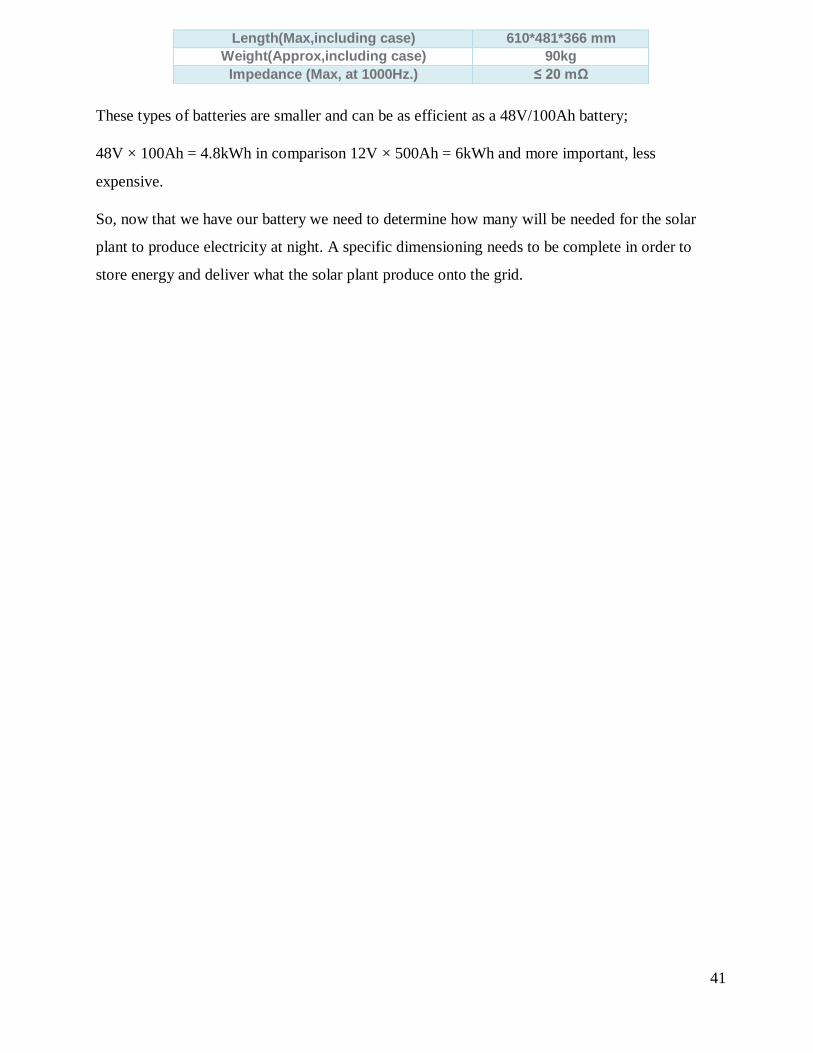
These types of batteries are smaller and can be as efficient as a 48V/100Ah battery;

48V × 100Ah = 4.8kWh in comparison 12V × 500Ah = 6kWh and more important, less

expensive.

So, now that we have our battery we need to determine how many will be needed for the solar

plant to produce electricity at night. A specific dimensioning needs to be complete in order to

store energy and deliver what the solar plant produce onto the grid.

Length(Max,including case) 610*481*366 mm

Weight(Approx,including case) 90kg

Impedance (Max, at 1000Hz.) ≤ 20 mΩ

42

Battery Basic Parameter

Voltage, Capacity and Energy Next, we need to familiarize ourselves with the basic parameters of a battery, and most

importantly the voltage and the capacity. Most PV batteries are rated at their nominal voltage;

12V, 24V, and 48V. Of course, the batteries placement in the PV system can attain any voltage

based on their interconnection with the system.

The next important parameter is the capacity, it refers to the amount of charge a battery can

deliver at the nominal voltage. The capacity is directly proportional to the number of electrodes

material

in the battery, this explain why a small cell has lesser capacity than a large cell based on the same

chemistry. The unit to measure capacity is Ah (Amper Hour);

𝑪𝒃𝒂𝒕𝒕 = 𝑰 × ∆𝒕.

In our case; our batterie has a 500Ah capacity.

One must not confuse between battery capacity and energy capacity; the latter is the total amount

of energy that a battery can store, it’s measured by the following equation:

𝑬𝒃𝒂𝒕𝒕 = 𝑪𝒃𝒂𝒕𝒕 × 𝑽𝒏

𝑬𝒃𝒂𝒕𝒕 = 𝟓𝟎𝟎𝑨𝒉 × 𝟏𝟐𝑽

𝑬𝒃𝒂𝒕𝒕 = 𝟔 𝟎𝟎𝟎𝑾

𝑬𝒃𝒂𝒕𝒕: is the energy available in the battery in (Watt hour)

𝑪𝒃𝒂𝒕𝒕 : is the capacity of the battery in (Ampere hour)

𝑽𝒏: is the nominal voltage in (Volt)

C-rate

If we take our battery with a capacity of 500Ah, it can theoretically deliver 500 A for a period of

1 hours at room temperature, but in reality, it’s not the case. In any type of battery, he C-rate is an

important

measure of discharge of the battery relative to its capacity. It’s determined by the current divided

by the battery capacity during one hour. For our battery, it has C-rate of 0.2 so it will give the

following current:

(12)

(13)

43

𝑰 = 𝑪𝒓𝒂𝒕𝒆 ×𝑪𝒃𝒂𝒕𝒕

𝟏𝒉

𝟎. 𝟐 ×𝟓𝟎𝟎 𝑨𝒉

𝟏𝒉= 𝟏𝟎𝟎𝑨

In this case it will take five hours in order for the battery to discharge.

And since 𝑰 =𝑪𝒃𝒂𝒕𝒕

∆𝒕 we can write the time as the battery fully discharge like so;

∆𝒕 =𝟏

𝑪𝒓𝒂𝒕𝒆

Storage Efficiency and Overall Battery Efficiency

Another high important component is the storage efficiency, it’s computed by taking the energy

storage output divided by the input of the system.

ŋ =𝑬𝒐𝒖𝒕

𝑬𝒊𝒏× 𝟏𝟎𝟎

Batteries are also known for two other kinds of efficiency that helps determine the overall battery

efficiency; Voltage efficiency and the Columbic efficiency.

ŋ𝒗 =𝑽𝒅𝒊𝒔𝒄𝒉𝒂𝒓𝒈𝒆

𝑽𝒄𝒉𝒂𝒓𝒈𝒆× 𝟏𝟎𝟎 , ŋ𝒄 =

𝑸𝒅𝒊𝒔𝒄𝒉𝒂𝒓𝒈𝒆

𝑸𝒄𝒉𝒂𝒓𝒈𝒆× 𝟏𝟎𝟎

ŋ𝒗 =𝟏𝟎𝑽

𝟏𝟐× 𝟏𝟎𝟎 , ŋ𝒄 =

𝟒𝟎𝟎𝑨

𝟓𝟎𝟎𝑨× 𝟏𝟎𝟎

Now we can compute the overall battery efficiency:

ŋ𝒃𝒂𝒕𝒕 = ŋ𝒗 × ŋ𝒄

ŋ𝒃𝒂𝒕𝒕 = 𝟎. 𝟖𝟑 × 𝟎. 𝟖 = 𝟔𝟔. 𝟒%

The battery efficiency reflects on all the effects of the chemical and electrical non-idealities

occurring in the battery.

SOC and DOD The State of Charge is defined as the percentage of battery capacity available for discharge and

can be computed with the following equation:

𝑺𝑶𝑪 =𝑬𝒂𝒗𝒂𝒊𝒍𝒂𝒃𝒍𝒆

𝑪𝒃𝒂𝒕𝒕 × 𝑽× 𝟏𝟎𝟎

(14)

(15)

(16)

(17) , (18)

(20)

(19)

44

On the other hand, Dept of Discharge is referred to the percentage of battery capacity that has

been discharged;

𝑫𝑶𝑫 =𝑬𝒅𝒊𝒔𝒄𝒉𝒂𝒓𝒈𝒆𝒅

𝑪𝒃𝒂𝒕𝒕×𝑽× 𝟏𝟎𝟎.

It’s important to note that these two are complementary, if we found a SOC of 80% then the

DOD should be 20% and vice versa.

Battery Cycles Life A very crucial parameter is the battery cycle; it can provide how many cycles the battery can be

charged and discharged before the capacity drops below 80% of the original value.

Figure 20: Battery Capacity Vs Cycles

Also, the cycle life depends heavely on the depth of discharge and temperature. The following

graph shows how theses component are related for a maintenance free Led Acid Solar battery.

Figure 22: Depth of Discharge Vs Cycle Numbers of a battery at given Temperatures

(21)

45

Clearly, the battery last longer in colder temperature not inferior to 20°C. Moreover, for a

particular temperature, cycle lifetime depends non-linearly on the depth of discharge; the smaller

the DOD, the higher the cycle life. However, such high cycle life can only be beneficial for a

small amount of discharge.

In other word, the battery could last longer if the average DOD could be reduced over its normal

operational cycle. In addition, battery overheating should be strictly avoided due to overcharging.

Battery Capacity and Temperature It should be also noted that the temperature affects the capacity of the battery, even though

temperature have a negative effect on cycle life, it is proportional to the capacity of the battery

during standard use as seen in the following graph.

Figure 23: Battery capacity Vs Temperature

We can notice that it’s possible to achieve an over capacity, but at such temperature, the life cycle

will be heavily affected and the battery will discharge rapidly.

Charging Controller If we do a direct coupling between a battery and a PV system we risk to damage the battery by

overcharging as there is no way to prevent it.

That’s why a charge controller is imperative in a battery storage PV system, it can help reduce

the losses by regulating the rate at which the battery is charging and discharging. It can also help

avoid overheating by cutting the PV power during hot days or prevent over-discharge by cutting

the battery from the load during cold periods.

Voltage regulations is helping the battery to perform under optimal conditions, for that the

voltage controller helps maintaining the voltage drain within specific range for a healthy

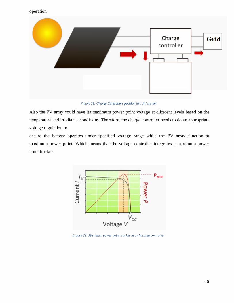
46

operation.

Figure 21: Charge Controllers position in a PV system

Also the PV array could have its maximum power point voltage at different levels based on the

temperature and irradiance conditions. Therefore, the charge controller needs to do an appropriate

voltage regulation to

ensure the battery operates under specified voltage range while the PV array function at

maximum power point. Which means that the voltage controller integrates a maximum power

point tracker.

Figure 22: Maximum power point tracker in a charging controller

47

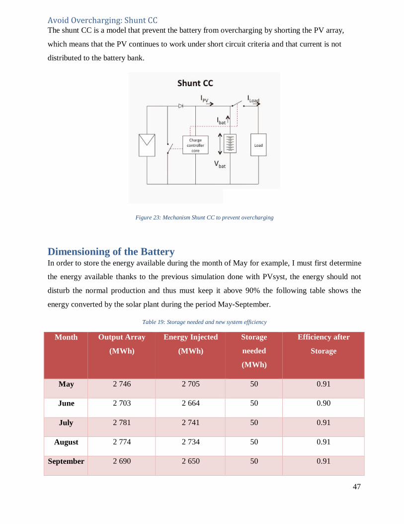
Avoid Overcharging: Shunt CC The shunt CC is a model that prevent the battery from overcharging by shorting the PV array,

which means that the PV continues to work under short circuit criteria and that current is not

distributed to the battery bank.

Figure 23: Mechanism Shunt CC to prevent overcharging

Dimensioning of the Battery In order to store the energy available during the month of May for example, I must first determine

the energy available thanks to the previous simulation done with PVsyst, the energy should not

disturb the normal production and thus must keep it above 90% the following table shows the

energy converted by the solar plant during the period May-September.

Table 19: Storage needed and new system efficiency

Month Output Array

(MWh)

Energy Injected

(MWh)

Storage

needed

(MWh)

Efficiency after

Storage

May 2 746 2 705 50 0.91

June 2 703 2 664 50 0.90

July 2 781 2 741 50 0.91

August 2 774 2 734 50 0.91

September 2 690 2 650 50 0.91

48

We will dimension our battery so they can release on a monthly average a capacity of 200MWh

per month, that is 6.7MWh per day to be injected on a discharge period of 5 hours. We know that

our battery can deliver 6kW of energy on a period of 5 hours, but we can’t just divide the energy

needed by this number to get how many batteries we must have, we need a proper dimensioning.

Standard conditions advise to dimension the battery bank as to obtain a nominal voltage of 48V

for strings with more than 1 600W, which means that we need to put 4 batteries of 12V in series.

Figure 24: Design of the batteries

We will dimension each battery bank for each string, the key element is the charge controller that

will help us determine the maximum and minimum current allowed.

Dimensioning of the charge controller

We need to make sure that the charge controller cope with the PV array system in order to charge

the batteries and avoid overcharge or discharge. We know that the power of the one string in our

PV system is 7 961W with a nominal voltage of 940.5V and 8.38A, and the voltage battery bank

is 48V.

So, by the basic equation: 𝑊 = 𝑉 × 𝐴𝑚𝑝𝑠

𝐴𝑚𝑝𝑠 = [𝑊 ÷ 𝑉]

𝐴𝑚𝑝𝑠 = 166𝐴

(22)

49

In other words, the charge controller should have a minimum current entry of 166A to avoid

damaging the battery bank. We need to oversize and choose a charge controller of 50V and 200A.

Figure 25: SUNWAY SWD48V200

Once the battery bank is fully charged the charge controller can turn on Shunt CC mode to avoid

overcharging. It takes normally 8 hours in order to charge a battery with an 80% state of charge,

but then we need to include some losses that will be encountered.

Losses Losses are inherent in any energy conversion process. Photovoltaic systems must provide the

necessary energy and compensate for the expected losses. These losses have several origins and

affect certain parameters of the system. The calculation of the power to be installed must therefore

integrate all the losses. We distinguish the following types of losses:

• PV losses = 0.8

• Loss of voltage = 0.9

• Efficiency Charge Regulator = 0.98

Losses at Charching : 0.7

Characteristics

Voltage Min: 600V

Current: 80 Amps

50

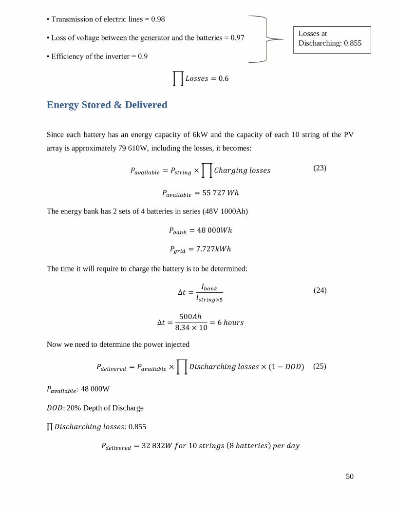
• Transmission of electric lines = 0.98

• Loss of voltage between the generator and the batteries = 0.97

• Efficiency of the inverter = 0.9

∏ 𝐿𝑜𝑠𝑠𝑒𝑠 = 0.6

Energy Stored & Delivered

Since each battery has an energy capacity of 6kW and the capacity of each 10 string of the PV

array is approximately 79 610W, including the losses, it becomes:

𝑃𝑎𝑣𝑎𝑖𝑙𝑎𝑏𝑙𝑒 = 𝑃𝑠𝑡𝑟𝑖𝑛𝑔 × ∏ 𝐶ℎ𝑎𝑟𝑔𝑖𝑛𝑔 𝑙𝑜𝑠𝑠𝑒𝑠

𝑃𝑎𝑣𝑎𝑖𝑙𝑎𝑏𝑙𝑒 = 55 727 𝑊ℎ

The energy bank has 2 sets of 4 batteries in series (48V 1000Ah)

𝑃𝑏𝑎𝑛𝑘 = 48 000𝑊ℎ

𝑃𝑔𝑟𝑖𝑑 = 7.727𝑘𝑊ℎ

The time it will require to charge the battery is to be determined:

∆𝑡 =𝐼𝑏𝑎𝑛𝑘

𝐼𝑠𝑡𝑟𝑖𝑛𝑔×5

∆𝑡 =500𝐴ℎ

8.34 × 10= 6 ℎ𝑜𝑢𝑟𝑠

Now we need to determine the power injected

𝑃𝑑𝑒𝑙𝑖𝑣𝑒𝑟𝑒𝑑 = 𝑃𝑎𝑣𝑎𝑖𝑙𝑎𝑏𝑙𝑒 × ∏ 𝐷𝑖𝑠𝑐ℎ𝑎𝑟𝑐ℎ𝑖𝑛𝑔 𝑙𝑜𝑠𝑠𝑒𝑠 × (1 − 𝐷𝑂𝐷)

𝑃𝑎𝑣𝑎𝑖𝑙𝑎𝑏𝑙𝑒 : 48 000W

𝐷𝑂𝐷: 20% Depth of Discharge

∏ 𝐷𝑖𝑠𝑐ℎ𝑎𝑟𝑐ℎ𝑖𝑛𝑔 𝑙𝑜𝑠𝑠𝑒𝑠: 0.855

𝑃𝑑𝑒𝑙𝑖𝑣𝑒𝑟𝑒𝑑 = 32 832𝑊 𝑓𝑜𝑟 10 𝑠𝑡𝑟𝑖𝑛𝑔𝑠 (8 𝑏𝑎𝑡𝑡𝑒𝑟𝑖𝑒𝑠) 𝑝𝑒𝑟 𝑑𝑎𝑦

Losses at

Discharching: 0.855

(23)

(24)

(25)

51

The following table will extend our findings, if we add another 10 strings set, here is how our

system will grow:

Table 20: Power delivered Vs Number of batteries Dimensioning

Power delivered per month

(MW)

Number of

Strings

Number of batteries Number of Charge

controllers

0.984 10 8 1

4.92 50 40 5

9.84 100 80 10

29.54 300 240 30

39.4 400 320 40

We used 14% of the total strings of the solar plant in order to produce approximatively 40MW of

stored energy, which means that the losses are too great and play a critical part in deciding the

energy stored.

Now we will move to the financial analysis and see if this system is more beneficial than a normal

grid connected.

Financial Analysis for the Batterie System

Initial Investment We will draw a table that includes all the new components for the system, their unit and their

price.

Table 21: Initial batteries and charge controller investment

Equipment Cost per unit

(MAD)

Number of Unit Total Cost (MAD)

Batteries 51 750 320 16 560 000

Charge controller 12 704 40 508 160

Cables 16 for 1m 800 12 800

Total 17 080 960

Currently, the kW price in Ifrane at high demands is 1.5 MAD when exceeding 500kW (according

to price-elec.ma), using this data, we can estimate the profit for one month to be: 59 100MAD. In

52

other words, in a period of 5 month we will generate: 295 500 MAD. The batterIES have an

expected life expectancy of 20 years and require low maintenance.

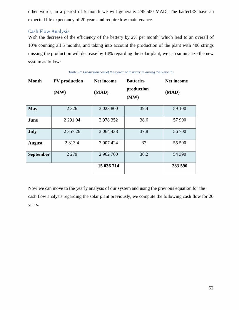
Cash Flow Analysis With the decrease of the efficiency of the battery by 2% per month, which lead to an overall of

10% counting all 5 months, and taking into account the production of the plant with 400 strings

missing the production will decrease by 14% regarding the solar plant, we can summarize the new

system as follow:

Table 22: Production cost of the system with batteries during the 5 months

Month PV production

(MW)

Net income

(MAD)

Batteries

production

(MW)

Net income

(MAD)

May 2 326 3 023 800 39.4 59 100

June 2 291.04 2 978 352 38.6 57 900

July 2 357.26 3 064 438 37.8 56 700

August 2 313.4 3 007 424 37 55 500

September 2 279 2 962 700 36.2 54 390

15 036 714 283 590

Now we can move to the yearly analysis of our system and using the previous equation for the

cash flow analysis regarding the solar plant previously, we compute the following cash flow for 20

years.

53

Table 23: cash flow analysis of battery system

Year Net income Accumulated

Cash Flow

NPV

1 283 590 538 821,00 - 17 080 960,00

2 255 231 768 528,90 - 16 797 370,00

3 229 708

975 266,01 - 16 258 549,00

4 206 737

1 161 329,41 - 15 490 020,10

5 186 063

1 328 786,47 - 14 514 754,09

6 16 7457

1 479 497,82 - 13 353 424,68

7 150 711

1 615 138,04 - 12 024 638,21

8 135 640

1 737 214,24 - 10 545 140,39

9 122 076

1 847 082,81 - 8 930 002,35

10 109 869

1 945 964,53 - 7 192 788,12

11 98 882

2 034 958,08 - 5 345 705,31

12 88 994

2 115 052,27 - 3 399 740,77

13 80 094

2 187 137,04 - 1 364 782,70

14 72 085

2 252 013,34 750 269,57

15 64 876

2 310 402,00 2 937 406,62

16 58 389

2 362 951,80 5 189 419,95

17 52 550

2 410 246,62 7 499 821,96

18 47 295

2 452 811,96 9 862 773,76

19 42 565

2 491 120,77 12 273 020,39

20 38 309

538 821,00 14 725 832,35

54

Despite not being beneficial, the battery will add value for the future year as additional revenue for

the PV

solar plant, as they will generate revenue during the night when demands are high.

STEEPLE Analysis

The STEEPLE analysis is a method to encompass the many side effect of this project and prove

that it will have positive impacts on society, the environment, job opportunities and so on. This

approach will strengthen the concept that Ifrane need a solar power plant.

Socio cultural: Alongside the domain of aeronautics, renewable energy is a growing field in

Morocco, every day we see more opportunity in Solar and wind energy careers with the openings

of new power plant. If implemented, this project will create work opportunities for people in the

rural area and internships for AUI students as well as workshops or class visits.

Technological: The usage of the latest technologies regarding photovoltaic panels as well as solar

batteries that are still being developed to maximize their potential.

Ecological: As seen previously, the solar plant reduces considerably the quantity of carbon dioxide

compared to a classical power plant with gaz.

Political: The government encourages private companies as well as the ONE to push their agendas

towards renewable and clean energy.

Legal: The Moroccan constitutional amendment n° 13 – 09 established on February the 11th 2010

has for objective to install a legal framework for any individual or institution willing to invest or

operate any type of facilities related strictly to renewable energy. The amendment also includes a

financial help plan, an environmental study, a sustainable development plan that will promote job

opportunities and proper infrastructure in the region.

Ethical: There is no idea which promotes that solar plant are a nuisance to society, every

developed country is trying to invest on PV energies even though they don’t have a high solar

irradiance, which proves their sense of duty regarding the future generations and how they will

leave this world impacted by pollution to them.

55

Conclusion

This Capstone Project consisted on giving realistic inputs and data to dimension a solar

photovoltaic station in Ifrane. The first phase of this work made it possible to pre-select the

various existing technologies on the market and to establish a preliminary choice of components,

based on the PVsyst software, in order to have the best production/price ratio. Indeed, the

comparison of technologies favored the use of polycrystalline 310 Wp, and a 1 MW inverter with

regards to the specifications.

After choosing the equipment and dimensioning the station with the right methodology to respect

a maximum output of 20MW, I found that the central will produce 30GWh/year and a

performance ratio of 82%. The financial analysis shows that the project is profitable and shows a

return on investment over a period of 8 years.

The next part was about including lithium ion battery in order to store energy during the day, and

sell it at night when demands are at their peak. For that we selected 2 sets of 4 batteries in series

with a total voltage of 48V and a capacity of 1000Ah. The energy stored during the first month

was approximately 40MW but unfortunately the project will not be profitable, it will benefit the

overall production over a certain time period only.

List of Equations

(1) Inverter Effciency

(2) Temperature loss

(3) Power injected

(4) Number of solar panels

(5) Inverter power compatibility

(6) Max number of modules in series

(7) Max numbers of panels in parallel

(8) Cross section of the cables

(9) Net Present value

(10) Cumulative Cash flow

56

(11) Performance Index

(12) Battery capacity

(13) Energy available in the battery

(14) C-rate Vs current

(15) Discharge rate

(16) Storage Efficiency

(17) Voltage Efficiency

(18) Columbic Efficiency

(19) Batterie efficiency

(20) State of Charge

(21) Depth of Discharge

(22) Volt amp Equation

(23) Power available

(24) Time of charge

(25) Power delivered

References Arno Smith, K. J. (2016). Solar Energy, the physics and engineering of photovoltaic conversion

technologies and systems. UIT Cambridge.

CIVIC SOLAR. (2015, July 17). Choosing the Correct Charge Controller. Retrieved from

https://www.civicsolar.com:

https://www.civicsolar.com/support/installer/articles/choosing-correct-charge-controller

D. Lalili, A. M. (2011). Input output feedback linearization control and variable step size MPPT

algorithm of a grid-connected photovoltaic inverter. Renewable Energy vol. 36, issue 12,

3282-3291.

Energy, M. o. ( February 12, 2014). Solar energy in India. Mumbai: Governement of India.

Kamelia, H. (2012). Modélisation d’une cellule photovoltaïque :étude comparative. Université

Mouloud Mammeri .

Marion, B. A. (1990). Photovoltaic Specialist Conference. Lake Buena Vista FL, pp.1601–1606.:

http://ieeexplore.ieee.org.

Masters, G. M. (2004). Renewable and Efficient Electric Power Systems. Stanford University .

57

NF-C-15-200, N. (2008). Le manuel technicien photovoltaïque . (PERACOD) .

Omar, B.-H. (2011). “Conception et réalisation d’un générateur photovoltaïque muni d’un

convertisseur MPPT pour une meilleur gestion énergétique “ . University Abou Bakr.

Rachid Chenni, E. M. (2011). Study of Solar Radiation in View Photovoltaic Systems

Optimization. Mentouri University: Smart Grid and Renewable Energy.

SMA. (2008). C15-712 : Installations Photovoltaïques. Union Technique de l'Electricité .

SMA. (2016). Solar Technology. http://www.sma-france.com.

Yilmaz, S. (2015). The analysis of different PV power systems for the determination of optimal PV

panels and system installation—A case study in Kahramanmaras. Science Direct.

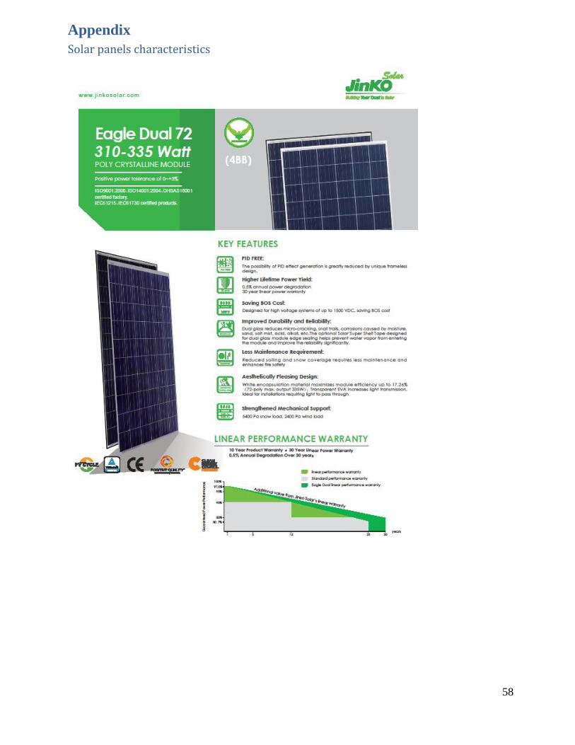
58

Appendix

Solar panels characteristics

59

60

Inverter characteristics

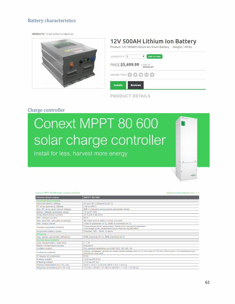
61

Battery characteristics

Charge controller