Embed Size (px)
Citation preview


TABLE OF CONTENTS
INTEGRITY TESTING - WHY, WHEN, HOW? .........................................................................................................6
OF BATS, MICE AND WAVES....................................................................................................................................11
THE SONIC METHOD .................................................................................................................................................14
BASIC PRINCIPLES .......................................................................................................................................................14
WAVES IN PRISMATIC RODS .........................................................................................................................................14
The wave equation................................................................................................................................................14
Reflection from the end.........................................................................................................................................17
Discontinuities in rods..........................................................................................................................................19
Damping...............................................................................................................................................................22
End rigidity...........................................................................................................................................................24
Conical rods .........................................................................................................................................................25
Sawtooth-profiled rods.........................................................................................................................................26
The PILEWAVE program.....................................................................................................................................27
Wave speed in concrete ........................................................................................................................................28
INSTRUMENTATION .....................................................................................................................................................30
PROCEDURE.................................................................................................................................................................33
Preparation for testing .........................................................................................................................................33
Testing ..................................................................................................................................................................34
Signal treatment ...................................................................................................................................................34
Presentation .........................................................................................................................................................35
Interpretation .......................................................................................................................................................36
Qualitative interpretation..................................................................................................................................................37
Quantitative Interpretation ...............................................................................................................................................56

2
Instrumented hammer analysis .........................................................................................................................................57
EVALUATION OF THE SONIC METHOD ..........................................................................................................................59
Capabilities ..........................................................................................................................................................59
Limitations............................................................................................................................................................60
Noise.....................................................................................................................................................................60
Accuracy...............................................................................................................................................................62
Frequency domain vs. Time domain.....................................................................................................................63
INTERNATIONAL COMPETITIONS ..................................................................................................................................64
SAMPLE SPECIFICATIONS .............................................................................................................................................64
ULTRASONIC TESTING .............................................................................................................................................67
BASIC PRINCIPLES .......................................................................................................................................................67
THREE-DIMENSIONAL WAVE PROPAGATION ................................................................................................................68
Attenuation ...........................................................................................................................................................69
Waves in an elastic half-space .............................................................................................................................71
Waves in Non-homogeneous Media .....................................................................................................................73
Normal incidence .............................................................................................................................................................73
Oblique Incidence ............................................................................................................................................................73
Media with inclusions...........................................................................................................................................74
INSTRUMENTATION .....................................................................................................................................................75
PILE PREPARATION ......................................................................................................................................................77
PROCEDURE.................................................................................................................................................................79
PRESENTATION OF THE RESULTS..................................................................................................................................80
INTERPRETATION .........................................................................................................................................................83
First arrival time (FAT) .......................................................................................................................................83
Fixed threshold.................................................................................................................................................................84
Dynamic threshold ...........................................................................................................................................................85
Moving windows (STA/LTA)..........................................................................................................................................85

3
Automatic FAT picking ...................................................................................................................................................86
Accuracy ..........................................................................................................................................................................87
Energy ..................................................................................................................................................................88
SPECIAL TECHNIQUES ..................................................................................................................................................89
Tomography .........................................................................................................................................................89
Simultaneous equations....................................................................................................................................................90
Fuzzy logic tomography...................................................................................................................................................92
Parametric tomography ....................................................................................................................................................93
Attenuation-based tomography ........................................................................................................................................94
Evaluation ........................................................................................................................................................................94
Single-hole testing ................................................................................................................................................96
SAMPLE SPECIFICATIONS.............................................................................................................................................98
RADIOACTIVE INTEGRITY TESTING .................................................................................................................100
REFERENCES..............................................................................................................................................................102

4
List of Figures
FIGURE 1: AN OBVIOUSLY DEFECTIVE PILE ..........................................................................................................................7
FIGURE 2: A BORED PILE CAST WITH BENTONITE .................................................................................................................8
FIGURE 3: DIAPHRAGM WALL CONSTRUCTED WITH POLYMER SLURRY................................................................................8
FIGURE 4: CARELESS TRIMMING OF A PILE HEAD .................................................................................................................9
FIGURE 5: PROPAGATION OF WAVES CAUSED BY A HAMMER IMPACT ON THE UPER LEFT-HAND CORNER...........................12
FIGURE 6: LONG VS. SHORT WAVES IN PILE TESTING..........................................................................................................13
FIGURE 7: WAVES IN AN ELASTIC ROD ...............................................................................................................................15
FIGURE 8: TWO OPPOSITE COMPRESSIVE WAVES MEETING AT X = L ..................................................................................18
FIGURE 9: A COMPRESSIVE WAVE MEETS A TENSILE WAVE AT X = L .................................................................................18
FIGURE 10: A ROD WITH A DISCONTINUITY ........................................................................................................................19
FIGURE 11: CHARACTERISTICS FOR A ROD WITH A REDUCED CROSS-SECTION (A2=A1/2, A3=A1) ......................................21
FIGURE 12: INFLUENCE OF SKIN FRICTION ON DOWNGOING WAVE .....................................................................................22
FIGURE 13: WAVES IN A CONICAL ROD ..............................................................................................................................26
FIGURE 14: PRISMATIC ROD WITH A SAWTOOTH PROFILE ..................................................................................................27
FIGURE 15: WAVE SPEED IN A CONCRETE ROD AS A FUNCTION OF GRADE AND AGE (FROM AMIR 1988) ...........................29
FIGURE 16: 3 REFLECTOGRAMS OF A 12 M LONG PILE (CA. 1980) ON THE OSCILLOSCOPE SCREEN (NOTE SECOND
REFLECTIONS) .......................................................................................................................................................30
FIGURE 17: MODERN EQUIPMENT FOR SONIC TESTING .......................................................................................................31
FIGURE 18: EUROPEAN (TOP) VERSUS AMERICAN (BOTTOM) CONVENTIONS .....................................................................35
FIGURE 19: ALTERNATIVE ZERO POINTS ............................................................................................................................36
FIGURE 20: QUANTITAVE INTERPRETATION USING PET SIGNAL MATCHING ......................................................................57
FIGURE 21: AN IDEALIZED MOBILITY PLOT ........................................................................................................................58
FIGURE 22: ATTENUATION OF ULTRASONIC WAVES IN CONCRETE ...................................................................................71
FIGURE 23: REFLECTION OF P-WAVES FROM THE BOUNDARY X = 0 ..................................................................................72
FIGURE 24: REFLECTION AND REFRACTION OF P- AND SV-WAVES ....................................................................................74
FIGURE 25: A P-WAVE HITTING A CYLINDRICAL INCLUSION ..............................................................................................75

5
FIGURE 26: THE CHUM SYSTEM FOR PILE INTEGRITY TESTING .........................................................................................76
FIGURE 27: ULTRASONIC TESTING INSTRUMENTATION .....................................................................................................76
FIGURE 28: RIGHT AND WRONG WAYS TO SEAL THE BOTTOM OF THE TUBES .....................................................................77
FIGURE 29: FAT PICKING BY FIXED THRESHOLD IN STRONG (LEFT – 10V SCALE) AND WEAK SIGNAL (RIGHT – 1V
SCALE) ..................................................................................................................................................................84
FIGURE 30: THE MOVING WINDOWS FAT PICKING METHOD...............................................................................................85
FIGURE 31: AUTOMATIC FAT PICKING ..............................................................................................................................86
FIGURE 32: INFLUENCE OF THE FIXED THRESHOLD ON THE FAT OBTAINED.......................................................................88
FIGURE 33: LOCATION OF DEFECTS IN A PILE .....................................................................................................................89
FIGURE 34: ULTRASONIC TOMOGRAPHY ............................................................................................................................89
FIGURE 35: THREE-DIMENSIONAL VISUALIZATION OF PILE ANOMALIES.............................................................................91
FIGURE 36: HORIZONTAL CROSS SECTION AT 20.4 M .........................................................................................................91
FIGURE 37: RESULT OF FUZZY LOGIC TOMOGRAPHY (LEFT) AND THE EXPOSED DEFECT (RIGHT) .......................................93
FIGURE 38: TOMOGRAPHY NEAR THE TOE - "BLIND" ZONE ................................................................................................95
FIGURE 39: STAGES IN REAL-TIME FUZZY-LOGIC TOMOGRAPHY ........................................................................................95
FIGURE 40: SINGLE HOLE TESTING.....................................................................................................................................96
FIGURE 41: SINGLE HOLE RESULTS ON A PILE WITH DINCONITUITY....................................................................................97
FIGURE 42: WAVE PROPAGATION THROUGH A PVC TUBE (LEFT) AND A STEEL TUBE (RIGHT) ...........................................98
FIGURE 43: RADIOACTIVE PROBE (SCHEMATIC) ............................................................................................................100

6
Integrity Testing - Why, When, How?
Everybody with experience in reinforced concrete construction has encountered columns
that, upon dismantling of the forms, exhibit air voids and honeycombing. Although these
columns may have been cast with good-quality concrete, in properly assembled forms
and with careful vibration, they still exhibit defects. Cast-in-situ piles are also columns,
but instead of forms made of wood or metal we have a hole in the ground. This hole may
pass through layers of dumped fill, loose sand, organic matter, and ground water, which
may be fast flowing or corrosive. Obviously, such conditions are not conducive to a
high-quality end product. The fact that on most sites we still manage to get excellent
piles is only a tribute to a dedicated team that makes this feat possible: The geotechnical
engineer, the structural engineer, the quantity surveyor, the contractor, the site
supervisor and the quality control laboratory. This is obviously a chain, the strength of
which is determined by the weakest link. This booklet is devoted to the last link - quality
control.
A flaw is any deviation from the planned shape and/or material of the pile. A
comprehensive list of events, each of which can lead to the formation a flaw in a pile
(Either cast-in-situ or driven) is presented by Fleming et al (1992): The use of concrete
that is too dry, water penetration into the borehole, collapse in soft strata, falling of
boring spoils from the surface, tightly-spaced rebars etc. In small diameter piles, dry
chunks of concrete may also get jammed in the reinforcement cage, creating large air-
filled voids (Figure 1). This is an interesting illustration of a flaw in a pile, which was
produced under ideal conditions: It was bored in hard clay above ground water level, and
then cast in the dry. If this could happen here, it could happen just anywhere and
according to Murphy’s Law, it certainly would.
The use of slurry in pile construction stabilizes the surrounding soil, but adds another
risk factor to the pile integrity (Figure 2). Diaphragm wall elements (barrettes),
invariably constructed under slurry, may also have imperfections (Figure 3).

7
Flaws may also develop after the piles have been cast. The use of explosives for nearby
excavation and careless trimming of the pile heads (Figure 4) are two common causes.
Therefore, we have to face the fact that on any given site some piles may exhibit flaws.
Of course, not all flaws are detrimental to the performance of the pile. Only a flaw that,
because of either size or location, may detract from the pile’s load carrying capacity or
durability is defined as a defect. The geotechnical engineer and the structural engineer
are jointly responsible to decide which flaw comprises a defect.
Figure 1: An obviously defective pile

8
Figure 2: A bored pile cast with bentonite
Figure 3: Diaphragm wall constructed with polymer slurry

9
Figure 4: Careless trimming of a pile head
The existence (Or non-existence) of flaws in piles often triggers a highly emotional
debate. Nevertheless, it is of utmost importance to handle this matter rationally and, at
the first stage, to gather maximum information as to the location, size and severity of all
flaws. This can be achieved with an integrity-testing program to be specified together
with the specification for pile construction (ICE 1996). With this information, we can
then arrive at a rational decision. This can be one of the following four options:
1. Disregard the flaw and accept the pile as-is
2. Accept the pile as a partial support and strengthen the superstructure
3. Repair the defective pile
4. Discard the defective pile altogether, and adopt proper remedial measures.
To be effective, the integrity testing program should take place as soon as this becomes
practical. For stress-wave methods, this means at a typical age of one week after casting.
Piles can be tested sooner under favorable conditions, but sometimes we have to wait
longer. One instance is when the concrete contains a larger-than-usual amount of

10
retarding admixture. The result should be reported as soon as the testing agency has had
ample opportunity to analyze and evaluate the results. To avoid unpleasant
misunderstandings, the specifications of the project should state, in no uncertain manner,
that the integrity test results should serve as an exclusive acceptance criterion.
The cost of a quality control program for a given site is very reasonable, and in any case
much lower than the potential loss caused by an undetected defect. The choice of a
testing firm should not be made on the lowest bidder basis, but shall take into account
the qualifications and record of the firm. In any case, the technical director of the firm
should be an experienced geotechnical engineer, well versed in the geology of soils,
piling techniques and wave propagation theory.

11
Of Bats, Mice and Waves
The final products of any piling operation (And in many cases the operation itself) are
practically invisible. You might even say that they are shrouded in complete darkness.
Under such conditions, judging the integrity of a finished pile may seem like a hopeless
task.
Not everyone, however, feels hopeless in the dark: Bats, for instance, are quite
comfortable! Their secret, as every child knows, is the clever utilization of sound waves.
Submarine sonar operators applied this technique decades ago, and piling people (being
naturally conservative) followed much later. The two techniques currently dominating
pile integrity testing, namely the sonic method and cross-hole ultrasonic method, both
utilize sound waves. Such waves travel not only in air and water, but also in solids,
where they are also called stress waves or elastic waves. We shall therefore begin with a
short introduction to the propagation of stress waves in solids. Later on, when dealing
with each of the testing methods, we shall review those principles of wave propagation
theory applicable to each specific method.
The last part provides an overview of other testing methods, not based on stress waves.
In this work, we shall use the term “pile” in the general sense. Thus, it will include all
deep foundations, whether driven, bored or augered. Specifically, the foundation types
called “caissons” “piers” and “drilled shafts” do belong to this category as well. Piles
may consist of concrete (cast in situ or precast), steel or wood.
When part of a solid body in a state of equilibrium is dynamically loaded at some point,
the effect of this load does not reach immediately all parts of the body. Due to inertial
effects, the stress and deformation caused by the load radiate from the point of
application at a finite speed towards all directions. Any given point in the body will be at
complete rest both before and after the effect of loading has passed it. This phenomenon,
illustrated in Figure 5, is defined as stress-wave propagation.

12
A A
1 millisecond
A A
4 milliseconds
A A
7 milliseconds
A A
10 milliseconds
Figure 5: Propagation of waves caused by a hammer impact on the uper left-hand corner
Waves are created not only by transient loading, but also by steady periodic loads.
Harmonic loading, where the load amplitude is a sinusoidal function of time, is a good
example. Since transient loads of any shape may be resolved by Fourier Transform into
a series of elementary harmonic waves, the theoretical treatment will by the same for
both.
The basic equation governing the relationship between wave propagation speed c,
wavelength λ and frequency f is:
c = λ.f Equation 1
13
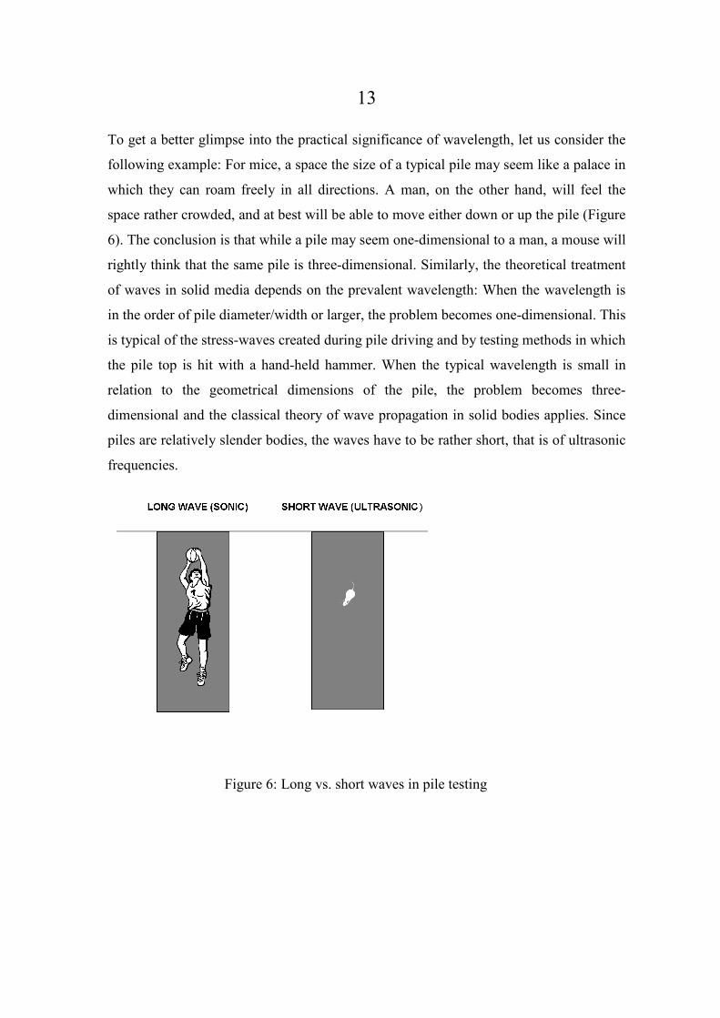
To get a better glimpse into the practical significance of wavelength, let us consider the
following example: For mice, a space the size of a typical pile may seem like a palace in
which they can roam freely in all directions. A man, on the other hand, will feel the
space rather crowded, and at best will be able to move either down or up the pile (Figure
6). The conclusion is that while a pile may seem one-dimensional to a man, a mouse will
rightly think that the same pile is three-dimensional. Similarly, the theoretical treatment
of waves in solid media depends on the prevalent wavelength: When the wavelength is
in the order of pile diameter/width or larger, the problem becomes one-dimensional. This
is typical of the stress-waves created during pile driving and by testing methods in which
the pile top is hit with a hand-held hammer. When the typical wavelength is small in
relation to the geometrical dimensions of the pile, the problem becomes three-
dimensional and the classical theory of wave propagation in solid bodies applies. Since
piles are relatively slender bodies, the waves have to be rather short, that is of ultrasonic
frequencies.
Figure 6: Long vs. short waves in pile testing

14
The sonic method
Basic Principles
The sonic method for the integrity testing of piles (ASTM 2007) is aimed at routinely
testing complete piling sites. To perform this test, a sensor (usually accelerometer) is
pressed against the top of the pile while the pile is hit with a small hand-held hammer.
Output from the sensor is analyzed and displayed by a suitable computerized instrument,
the results providing meaningful information regarding both length and integrity of the
pile. The sonic test is fast and inexpensive, with less than a minute needed to test a given
pile (Amir & Amir 2008).
To have a better understanding of the inner workings of the method, let us first go
through the basics of one-dimensional wave propagation in prismatic rods. We shall then
discuss the specific instrumentation, go through the interpretation and end this chapter
by discussing the capabilities and limitations of the method.
Waves in prismatic rods
The wave equation
Since piles do basically resemble prismatic rods, the analysis of waves in prismatic rods
is evidently of much importance to those involved in driving piles and in testing them.
The mathematics involved is fairly basic, provided we first make a few reasonable
assumptions:
The wavelength is equal to or larger than the pile diameter.
The rod is prismatic with a constant cross-section A, elastic with Young’s Modulus E and
homogeneous with mass density ρ.
Cross sections remain plane, parallel and uniformly stressed.
Lateral inertia effects are negligible.

15
Let us now examine an element ∆x along the rod (Figure 7). If we denote the stress
above the element by σ and below the element by σ+(∂σ/∂x) ∆x, the unbalanced force
on the element is (∂σ/∂x) ∆x. If we denote particle displacement by u, the particle
velocity is given by ∂u/∂t, the particle acceleration by ∂2u/∂t2 and the strain ε by ∂u/∂x.
According to Newton’s second law (Force equals mass times acceleration),
dx
σσσσ
σσσσ ∂σ∂σ∂σ∂σ ∂∂∂∂++++ ( / )x dx
x
A
Figure 7: Waves in an elastic rod
A (∂σ/∂x) ∆x = A. ∆x.ρ.∂2u/∂t2 Equation 2
Because of elasticity, σ = E.∂u/∂x (Hooke's Law). Substituting in and eliminating both
A and ∆x on both sides, we get:
xuxuE ∂∂=∂∂ // 222 ρ Equation 3
or:

16
∂∂
∂∂
2
22
2
2
u
tc
u
x= ⋅
Equation 4
where
c2 = E/ρ Equation 5
This is the well-known wave equation in one dimension. The general solution of this
differential equation, due to D’Alembert, is the sum of two functions having the
following form:
u = f(x-ct) + g(x + ct) Equation 6
We can easily verify the validity of this solution by substitution. To understand the
physical significance of this solution, let us consider the first term in Equation 6,
assuming the argument x-ct is constant. In such a case, the function f(x-ct) is also
constant. If we wish to keep it constant, we have to increase x by c.∆t when t is
increased by ∆t. This means that f describes a wave with a constant form, moving in the
positive x direction at a constant speed c. Likewise, g describes a wave moving at the
same speed, but in the opposite direction. Both f and g are determined by the initial
conditions.
From Equation 6, the particle velocity v is equal to f ’(x - ct) + g ’(x + ct). For the sake
of simplicity, we shall in the following consider only the outgoing wave, thus v = -f.c.
We may further omit the minus sign if we assume the compressive wave to be positive.
The force acting on a given cross-section is:
P = σ.A = ε.E.A = (EA/c)v = Z.v Equation 7

17
This means that the force acting on any section in the rod at a given moment is
proportional to the particle velocity. Z is defined as the impedance of the section with
typical dimensions of kg/sec. Other expressions for the impedance are Z = A.(Eρ)½ or Z
= ρ.c.A.
As we mentioned before, this relation is true only for the outgoing waves, while for
returning waves, P = -Z.v.
A word of caution: particle velocity v and wave speed c are two distinct entities:
Particle velocity v is a function of the initial conditions, such as the blow intensity. The
particle velocity caused by tapping with a handheld hmmer will be much lower than that
caused by a large piledriving hammer. The wave speed c, on the other hand, depends
only on the material constants E and ρ of the pile, and will therefore be identical in both
cases.
Reflection from the end
When waves move in a finite rod, they will eventually reach the end x = L. The wave
will be reflected from the end, the nature of the reflection depending on the boundary
conditions at the end.
When the end is fixed, u (L, t) = 0. In this case, the wave will be reflected unchanged, by
which we mean that a compressive wave will be reflected as compressive, and vice
versa.
We can prove this result without any recourse to mathematics. Although infinite rods are
rather uncommon in practice, they are quite useful in theory: Let us then try and
visualize an infinite rod in which two compressive waves of equal shape are approaching
the point x = L from both sides (Figure 8). When the two waves meet, the

18
displacements associated with them will cancel each other, so that the point x = L will
stay stationary. This obviously satisfies the boundary conditions.
The stresses at this point, however, will add up and reach twice the normal value. An
observer on either side will conclude that a compressive wave will be reflected
unchanged from the fixed end. The same reasoning, by the way, also holds for tensile
waves.
Figure 8: Two opposite compressive waves meeting at x = L
Figure 9: A compressive wave meets a tensile wave at x = L
If one of the meeting waves is compressive and the other one tensile (Figure 9) the
stresses will mutually cancel at x = L. This conforms to the boundary condition at a free
end σ(L,t) = 0. Since the particle velocities associated with both waves are directed to
the right, they will add up at x = L, doubling the normal particle velocity.

19
The tensile wave in Figure 9 will continue moving to the left, wile the compressive wave
will travel to the right. Our faithful observer will reach the inevitable conclusion that a
wave reflected from a free end will change sign: From compressive to tensile, and vice
versa.
If we take a prismatic rod with a given length L, and apply a dynamic load to the end
x=0, the wave created will travel along the rod and return, the duration of the whole trip
T = 2L/c.
Discontinuities in rods
A discontinuity in a rod is defined as an abrupt change in either cross section (From A1
to A2) or material properties E and ρ. When a wave traveling in a rod meets such a
discontinuity, one part of it will be reflected back while another part will go on beyond
the discontinuity (Figure 10). Let us represent the incident wave parameters by the index
i, while r and t will denote the reflected and transmitted waves, respectively.
Figure 10: A rod with a discontinuity
From equilibrium:

20
A ( + ) = A 1 i r 2 tσ σ σ Equation 8
Moreover, from continuity:
tri v= v- v Equation 9
Since v = ±σA/Z, Equation 9 may be re-written as:
(A / Z ).( - ) = (A / Z ). 1 1 i r 2 2 tσ σ σ Equation 10
From Equations 10 and 8 we get the following relationships:
irZZ
ZZσσ .
21
21
+−
−= Equation 11
and:
σ σt i
Z
Z Z
A
A=
+2 2
1 2
1
2 Equation 12
These two equations enable us to calculate the behavior of a wave as it moves along a
rod of an arbitrary shape. A convenient way to visualize the process is by using the

21
method of characteristics, due to Riemann, which represents the wave propagation in the
x-t plane.
As we have already seen, the solution of the wave equation is in the form of f(x - ct) and
g(x + ct). If the functions f and g are constant, these solutions describe two sets of
straight lines in the x-t plane with a slope of c (downward) and -c (upwards),
respectively. These lines are called characteristics.
Figure 11 shows the characteristics for a rod with a reduced cross-section. The figures
besides the lines are the respective stresses, calculated from Equations 11 and 12.
Using the method of characteristics we draw a graph showing the velocity at the top
versus time. Such a graph is called a reflectogram.
Figure 11: Characteristics for a rod with a reduced cross-section (A2=A1/2, A3=A1)
(After Vyncke & van Nieuwenburg 1987)

22
Damping
All former analyses of wave phenomena in prismatic rods were based on the assumption of
zero skin friction. When the rod is embedded in some solid material, however, the situation
is different: Rod particle displacement, which is associated with the wave, will give rise to
skin friction forces in the opposite direction. To visualize the effect of these forces, let us
consider the case of a compressive wave traveling downwards in a rod (Figure 12):
Figure 12: Influence of skin friction on downgoing wave
The equilibrium condition means that:
P - P - F = 01 2 Equation 13

23
Because of compatibility, v1 = v2. If there is no change in the impedance of the rod,
Z1=Z2, therefore P1= -P2. If we substitute this in the equilibrium equation, we get:
P = - P = F / 21 2 Equation 14
This means that the friction force F gives rise to a pair of waves, each equal in
magnitude to F/2: A reflected compressive wave and a transmitted tensile wave.
The reflected wave is of the same type of the incident wave: A compressive wave will
cause a compressive reflection, and vice versa. Thus, the reflection due to skin friction is
similar to an increase in the impedance.
The transmitted component P2 is superposed on the incident wave. Since P2 is of
opposite sign, the net result is a weakening, or damping, of the wave. The total energy in
the rod is decreased, the difference being radiated to the surrounding medium.
Let us assume that the surrounding medium acts as a linear viscous material, that is:
F = η C v Equation 15
where F is the friction developed per unit length, C is the perimeter of the rod and v the
particle velocity. The incident wave is associated with an internal force P = Z.v, reduced
by ∆P due to friction. The ratio between the transmitted and the incident force is:
R = 1 - ∆P/P = 1 - F/2Zv = 1 - ηCv/2A(Eρ)1/2v = 1 - [(Cη/2A)
.(Eρ)1/2] Equation 16
For a rod with either a circular or a square cross section, C/A = 4/D and then R becomes

24
1-[2Cη/D.(Eρ) 1/2]. If the length of the rod is L, a dynamic force P0 applied to one end
will arrive at the other end as:
PL = P0 RL ≅ P0 e
-k Equation 17
Where k = (L/D).[2η/(Eρ)1/2]. Clearly, a small increase in the L/D ratio will lead to a
sharp decrease in the force (or velocity) reaching the end. The important contribution of
L/D ratio to damping is therefore apparent.
For a linear visco-elastic medium surrounding the rod, the friction is given by.
η(∂u/∂t)+ku. For harmonic waves, Novak et al. (1978) suggested the following
parameters:
η π ρ= D G s and k = 2G, where G and ρs are the shear modulus and the density of the
surrounding medium, respectively.
With known damping parameters, we can correct the characteristics (and the resulting
reflectogram) accordingly.
End rigidity
So far, we have dealt with two extreme boundary conditions: A free end and a fixed end.
In reality, however, we often encounter ends with a finite rigidity. For the sake of
simplicity, let us assume that the medium beyond the end exhibits a linearly viscous
behavior. In such a case, the stress σ developed in the medium is proportional to the
particle velocity v:
σ = η.v Equation 18
If the area of the end is A, the force developed is P = Aηv. The impedance of the end is
equal to the ratio between the force and velocity, that is:

25
Ze = P/v = Aη Equation 19
The impedance of the rod directly near the end is Zr = ρcA. Thus, the impedance ratio is:
Ze/Zr = η/ρc Equation 20
If η >> ρc the end will behave as a fixed end and if η << ρc the end will respond as a
free end.
In the special case when η = ρ c there will be no reflection from the end.
Vyncke & van Nieuwenburg (1987) studied the case of an end with an elastic behavior.
They concluded that the reaction of the spring is frequency-dependent: For high
frequencies the end is practically free, while for low frequencies it is fixed. A mixed
transient pulse will thus be distorted upon reflection.
Conical rods
In many cases we may encounter rods where the cross section increases (or decreases)
gradually. Such a situation occurs in conical piles, as well as in the lower part of
underreamed (belled) piles. The simplest idealization of such a situation is the straight
conical rod (Figure 13) in which the cross-sectional area of such a cone is given by:
A(x) = A .x / a0
2 2
Equation 21
this problem was solved for a small cone angle Ω , in which the stresses on any spherical
surface (r constant) are uniform and parallel. The analysis is similar to that for a straight
rod, however the relation between stress and velocity is not linear as it was for the
straight rod. In fact, the impedance Z = P/v is now a complex function of, among other
things, the coordinate x and the wavelength λ.

26
Figure 13: Waves in a conical rod
When a pulse is moving down a prismatic rod that widens into a cone (underream), we
can expect some form of reflection, indicating an increase in impedance. The nature of
the reflection depends on both the cone angle and the wavelength: A small angle may
create no reflection, while a large angle will. Furthermore, small wavelengths will pass
unhindered, while longer waves will be almost fully reflected. The reflected pulse may
miss some of its higher frequencies, and may thus look quite different from the incident
wave.
Sawtooth-profiled rods
Certain piling techniques produce a pile that has a sawtooth profile (Figure 14). We may
regard this as a special case of the straight rod with a series of enlargements and
constrictions, together creating a multitude of reflections and refractions. Unlike the case
of the straight rod, the reflectogram here will show almost no reflection at t1=2L/c.
Instead, it will show a strong reflection after a longer time t2>t1. The reason for this is as

27
follows: For a typical situation, the wave that travels straight thorough the obstacle
course will look like a recruit after an obstacle course: very weak indeed. The stronger
reflection we see at t2 is, in fact, a combination of different waves that have already been
reflected and transmitted several times on the way. Clearly, this takes some more time,
so that naturally t2>t1.
Figure 14: Prismatic rod with a sawtooth profile
The sawtooth rod, like its conical counterpart, acts like an acoustic filter, letting high
frequencies pass while stopping low frequencies (Vyncke & van Nieuwenburg 1987).
The PILEWAVE program
The PILEWAVE computer program (Amir 1995), attached to this book, runs on any PC
under Windows operating system. Using PILEWAVE, we can simulate wave
propagation in rods of different shapes. The pile shape library included in the program
consists of many typical shapes, from a straight cylinder to a sawtooth profile. In
addition, we can use the mouse (An unavoidable creature when dealing with waves) to
draw any rod profile we like. The program then plots the characteristics, enabling us to

28
follow the waves as they are reflected and transmitted. As a bonus, we also obtain the
resulting reflectogram.
Additional features of the program are the option to change both skin friction and
amplification. When we have high skin friction, the toe reflection may become very
weak. Under such conditions, we must apply exponential amplification to compensate
for the damping and obtain a clear, well-balanced reflectogram.
Wave speed in concrete
Most piles are probably manufactured of concrete, either cast-in-situ or precast.
Therefore, the velocity of wave propagation in concrete should be of much interest to us.
As we have already demonstrated, the wave speed in a rod is given by c E= / ρ . The
mass density ρ is determined at the moment of concreting, and thence does not change.
Young’s Modulus, on the other hand, tends to increase as the concrete hardens, albeit at
a decreasing rate. As a result, c increases with the age of the concrete
Figure 15 gives a relationship between c and the age of the concrete for three common
concrete grades (Amir 1988). We can see that from the age of one week onwards, c lies
between the rather narrow limits of 3,600 and 4,400 m/sec, or 4,000m/sec ± 10%. This
means that whenever we have no information regarding the concrete, assuming a speed
of 4,000 m/sec is an excellent first guess.
The general relation between concrete compressive strength and wave speed is given by
(Amir 1988):
6/1
cKfc = Equation 22

29
Figure 15: Wave speed in a concrete rod as a function of grade and age (From Amir 1988)
When testing piles on a large site, we have to remember that different piles have
different ages. Moreover, in many cases the concrete used for piles contains an
admixture for retarding its hardening. Small differences in the content of retarder may
influence the rate of hardening. As a consequence, we find ourselves in a situation where
each pile has its specific wave speed. Statistical analysis of a piling site (Klingmuller
1992) showed that actual wave speed varied between 2,500 and 6,000 meters per second.
While the lower limit may be explained by the age of the concrete, only poor data can
explain the higher values. Since the real speed for every pile is usually unknown, we
have to compromise by assuming a site-average velocity, and accepting an error of
±10% in the reported lengths.

30
Instrumentation
Steinbach & Vey (1975), who used a makeshift system consisting of an oscilloscope and
amplifiers, were probably the first to investigate the sonic test. Although their results
look pretty crude by modern standards, they were still able to get a rather convincing
reflection from the toe.
The first-generation of commercial pile-testing equipment, which soon followed, still
consisted of purely analog components, based on an oscilloscope and a Polaroid camera.
A typical result from such a system is shown in Figure 16.
Figure 16: 3 reflectograms of a 12 m long pile (ca. 1980) on the oscilloscope screen (note
second reflections)

31
The early eighties saw the transition to the second-generation: Digital systems based on
purpose-built computers and some proprietary operating system. Third-generation
equipment appeared a few years later, once ruggedized laptop computers became
commercially available, and used some version of DOS. Today, practically all testing
systems in use are computerized, belonging to either second or third generation.
Fourth-generation testing equipment, which recently became available, makes optimum
use of the accelerated progress in both computing power and software capabilities, with
a heavy accent on the software aspect. It runs under the worlds’ most popular operating
system (MS-WINDOWS), with all the resulting advantages.
With modern systems, the sonic test can provide us with more information than just the
actual pile length: Changes in cross-section, the existence of inclusions, cracks and other
discontinuities, poor concrete quality, amount of fixation of the toe, etc.
A modern system for sonic testing of piles (Figure 17) consists of the following
components:
Figure 17: Modern equipment for sonic testing

32
A suitable wave generator. In spite of the impressive name, what it means in fact is a
good-quality nylon hammer with replaceable tips (They quickly wear out when hitting
rough concrete).
A transducer which is pressed against the top of the pile and is sensitive to motion. The
transducer serves both to trigger the system when it senses the hammer blow, and
subsequently to receive all the reflections. This item should be very sensitive and at the
same time very rugged. Commercial accelerometers are particularly suited to this task.
An analog-to-digital (A/D) converter, which turns the continuous analog signal from the
accelerometer into a discrete series of numbers a computer can analyze. The A/D
converter should have a 12-bit dynamic range, so it can handle signals as small as
1:4000 of the maximum.
A portable computer. There is a vast selection of notebook computers one can take to a
site, but only a handful that will survive a large number of such trips. These “hard-hat”
computers should be immune to dust and occasional spray, and have screens that will
not fade under direct sunlight.
Dedicated software that handles the input and displays the results in a form that is easy
to interpret. The usual presentation of the results is of pile-head velocity vs. time, or
time-domain presentation. As a rule, the time axis is multiplied by c/2 and thus
transformed to length base. This form is also called a reflectogram.
An optional component of the sonic equipment is the instrumented hammer, included in
certain systems. The instrumented hammer contains an internal force transducer, which
measures the force created when the pile head is hit. The time-history of the force is then
stored in the computer for further analysis.

33
Procedure
Preparation for testing
The minimum age for testing is often quoted as five days after casting. There are,
however, exceptions both ways to this rule: In soft soils, and when the top is smooth,
meaningful testing can be performed even on the next day. On the other hand, when the
soil is hard and the concrete includes an excessive amount of retarder, testing should be
postponed accordingly.
The hammer blow, which forms the input for the test, should be sharp and uninterrupted.
This requires first of all free access to the top of the pile. If, for any reason, the pile was
not cast to ground level the contractor should excavate a suitable pit around it to allow
accessibility. The spiral reinforcement above the concrete should be removed, as should
any soil heaped on the pile.
The second condition is that the exposed concrete should be of full strength, clean and
dry. In most cases, this is not the situation: For piles cast under slurry, the top will
usually contain a low-strength mixture of concrete and slurry. In augered (CFA) pile the
insertion of the reinforcement will cause segregation and bleeding reaching the top.
Even when the piles are cast in the dry the surface of the concrete is exposed to direct
sunlight without proper curing, causing the concrete to dry up. For this reason, the upper
part of the concrete should be trimmed off until good quality concrete is reached. The
exact amount which is to be removed cannot be determined in advance, and in some
cases may exceed one meter. Once this operation is complete, all loose chunks of
concrete should be removed. The pneumatic jackhammer is ideally suited for this
purpose: It is powerful enough to be cost effective, but not too much as to damage the
pile. In addition, compressed air is useful for flushing the surface after the breaking stage
and removing all the debris.
Under difficult testing condition (High friction, high L/D values) preparing a small
testing surface with a disc grinder may be very beneficial.

34
Testing
Testing is carried out by pressing the transducer to the pile head and hitting the concrete
with a plastic hammer. For good coupling, a small amount of suitable putty (such as
HBM AK-22) should be spread on the bottom of the transducer. The transducer records
the reflected waves and the results are further processed by the computer. The output for
all piles shall clearly identify the project, pile number, date, time, depth scale and wave
speed on which the measurements are based, as well as the results of at least three
similar hammer blows.
Signal treatment
The analog output from the accelerometer is first turned into a digital signal by a suitable
A/D converter. This component is located inside the digital transducer or, if an analog
tranducer is used, in a special circuit which is attached to the computer.
To turn the raw data into an acceptable reflectogram, the software must go through the
following operations, some of which are performed automatically, while others are done
interactively by the operator:
Integration: The input must be converted from acceleration to velocity
Filtering: To eliminate high-frequency noise and obtain a smooth curve
Rotation: The curve is turned so that the area enclosed between it and the horizontal axis is
minimized.
Amplification: Because of friction damping, the stress wave is weakened as it progresses. To
obtain a legible reflectogram, it has to be compensated for damping, usually exponentially.
Certain system also allow for linear amplification, which enhances the upper part of the pile. In
a well-balanced reflectogram, the reflection from the toe has the same amplitude as the hammer
blow on the top.
Normalization: No two blows are equal in intensity, so that the resulting velocities differ too. In
order to assist understanding of the results, the vertical scale is adjusted so that the maxima and
minima of the reflectogram occupy most of the available vertical space.
35
Averaging: A typical reflectogram will include a consistent component (signal) and a random
component (noise). As a result, no two blows will yield the same reflectogram. To enhance the
resolution of the system, it should include an option for the averaging of successive signals.
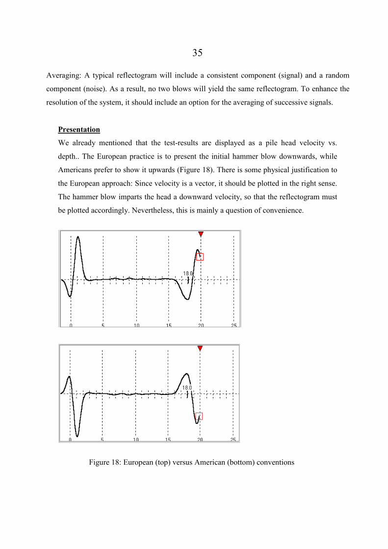
Presentation
We already mentioned that the test-results are displayed as a pile head velocity vs.
depth.. The European practice is to present the initial hammer blow downwards, while
Americans prefer to show it upwards (Figure 18). There is some physical justification to
the European approach: Since velocity is a vector, it should be plotted in the right sense.
The hammer blow imparts the head a downward velocity, so that the reflectogram must
be plotted accordingly. Nevertheless, this is mainly a question of convenience.
Figure 18: European (top) versus American (bottom) conventions
36
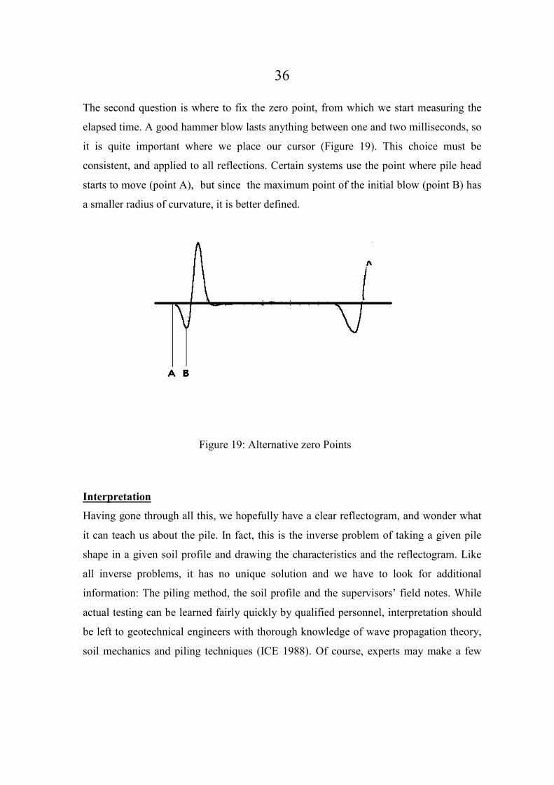
The second question is where to fix the zero point, from which we start measuring the
elapsed time. A good hammer blow lasts anything between one and two milliseconds, so
it is quite important where we place our cursor (Figure 19). This choice must be
consistent, and applied to all reflections. Certain systems use the point where pile head
starts to move (point A), but since the maximum point of the initial blow (point B) has
a smaller radius of curvature, it is better defined.
Figure 19: Alternative zero Points
Interpretation
Having gone through all this, we hopefully have a clear reflectogram, and wonder what
it can teach us about the pile. In fact, this is the inverse problem of taking a given pile
shape in a given soil profile and drawing the characteristics and the reflectogram. Like
all inverse problems, it has no unique solution and we have to look for additional
information: The piling method, the soil profile and the supervisors’ field notes. While
actual testing can be learned fairly quickly by qualified personnel, interpretation should
be left to geotechnical engineers with thorough knowledge of wave propagation theory,
soil mechanics and piling techniques (ICE 1988). Of course, experts may make a few

37
learned mistakes from time to time, but the ignorant make a lot of stupid mistakes all the
time. Expert interpretation is hence the key to successful sonic testing,
Qualitative interpretation
The first step in analyzing the reflectogram is qualitative, and is performed immediately
following each test. This is done by mentally comparing the graph to a catalogue of
various pile shapes and their respective reflectograms (Rausche et. al 1988). Some
typical cases are presented in Table 1.
If our graph falls into one of these categories (except for the last one, of course), it
means that we can explain the significance of what we have in hand. If the opposite is
true, we have to try another spot on the pile. Although theoretically the exact location we
hit is of no significance (Fukuhara et al. 1992), in practice different spots react
differently. If all our attempts fail, either the pile top was not sufficiently prepared for
testing, or the specific pile is just not amenable to sonic testing.
On the basis of qualitative interpretation Klingmuller (1992) divided all the piles on a
site into six categories: Piles belonging to classes 1 to 4 were accepted without
reservation, class 5 piles were considered as candidates for dynamic load testing prior to
acceptance and those belonging to class 6 were rejected altogether.

38
Table 1: Typical piles with respective reflectograms
PILE PROFILE
DESCRIPTION
REFLECTOGRAM
Straight pile,
Straight pile,
Straight pile,
Increased
Decreased
Locally
Locally

39
High L/D ratio
Multiple
reflections from
Irregular profile
Table 2 presents Four typical examples of reflectograms obtained using the PET system
on 600 mm diameter bored piles. All piles were bored to an approximate depth of 11 m.
The examples show, in that order:
A normal pile
A pile with an enlarged cross section (collapse during boring)
A pile with necking (collapase during casting)
A pile not amenable to interpretation due to an ill-prepared head.

40
Table 2: Examples of Sonic Test Results
P
I
L
E
L
e
n
g
t
h
(
m
)
D
et
ai
ls
Graph Rema
rks
C
3
1
1
1
.
6
D
at
e:
2
0
0 2 4 6 8 10 12 14
No
anom
alies

41
P
I
L
E
L
e
n
g
t
h
(
m
)
D
et
ai
ls
Graph Rema
rks
0
2-
0
8-
0
8

42
P
I
L
E
L
e
n
g
t
h
(
m
)
D
et
ai
ls
Graph Rema
rks
c
=
4
0
0
0

43
P
I
L
E
L
e
n
g
t
h
(
m
)
D
et
ai
ls
Graph Rema
rks
A
m
p
=
2
6

44
P
I
L
E
L
e
n
g
t
h
(
m
)
D
et
ai
ls
Graph Rema
rks
X
2
1
2
A
1
1
.
1
D
at
e:
2
0
0
0 2 4 6 8 10 12 14
Increa
sed
cross
sectio
n @
5m

45
P
I
L
E
L
e
n
g
t
h
(
m
)
D
et
ai
ls
Graph Rema
rks
2-
0
5-
1
2
c

46
P
I
L
E
L
e
n
g
t
h
(
m
)
D
et
ai
ls
Graph Rema
rks
=
4
0
0
0
A

47
P
I
L
E
L
e
n
g
t
h
(
m
)
D
et
ai
ls
Graph Rema
rks
m
p
=
2
1

48
P
I
L
E
L
e
n
g
t
h
(
m
)
D
et
ai
ls
Graph Rema
rks
C
3
6
? D
at
e:
2
0
0
0 2 4 6 8 10 12 14
Necki
ng @
4.2m
– no
toe
reflect

49
P
I
L
E
L
e
n
g
t
h
(
m
)
D
et
ai
ls
Graph Rema
rks
2-
0
8-
0
8
c
ion

50
P
I
L
E
L
e
n
g
t
h
(
m
)
D
et
ai
ls
Graph Rema
rks
=
4
0
0
0
A

51
P
I
L
E
L
e
n
g
t
h
(
m
)
D
et
ai
ls
Graph Rema
rks
m
p
=
5
5

52
P
I
L
E
L
e
n
g
t
h
(
m
)
D
et
ai
ls
Graph Rema
rks
C
2
3
? D
at
e:
2
0
0
0 2 4 6 8 10 12 14
Head
not
clean
– no
toe
reflect

53
P
I
L
E
L
e
n
g
t
h
(
m
)
D
et
ai
ls
Graph Rema
rks
2-
0
7-
1
8
c
ion

54
P
I
L
E
L
e
n
g
t
h
(
m
)
D
et
ai
ls
Graph Rema
rks
=
4
0
0
0
A

55
P
I
L
E
L
e
n
g
t
h
(
m
)
D
et
ai
ls
Graph Rema
rks
m
p
=
1
0

56
Quantitative Interpretation
When both the form of the pile and the skin friction distribution are known, a synthetic
reflectogram may be drawn using Equations 11, 12 and 14. The inverse problem,
however, has no unique solution even for the zero-friction case (Vyncke & van
Nieuwenburg 1987, p. 15, Danziger et al. 1976). Approximate solutions may be
obtained by signal-matching techniques (Middendorp & Reiding 1988 p. 33-43) which
work as follows:
First, a reference reflectogram for a cylindrical pile is chosen. In certain cases, such a
reference reflectogram may be obtained by averaging a large number of reflectograms
over a given site.
The soil friction function is then varied until the synthetic reflectogram calculated for a
cylindrical pile is identical to the reference reflectogram.
Using the friction distribution thus obtained, the pile profile (or rather impedance
profile) is varied until a good match is reached for the pile under consideration. Under
ideal conditions, this profile may be close enough to the real one. The signal matching
described above can be performed either interactively or automatically (Courage &
Bielefeld 1992 pp. 241-246) but both methods are subject to the same limitations.
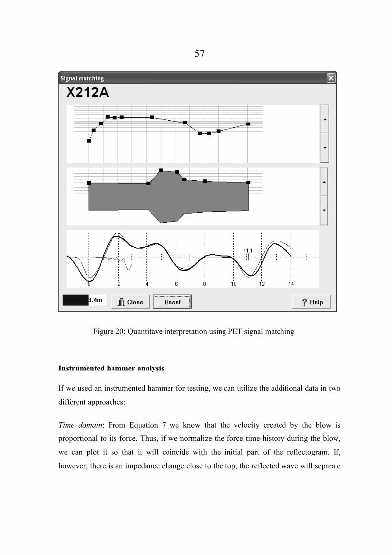
Figure 20 is an example of signal matching performed by the PET software. The PET
signal matching tool uses drag and drop method to draw both the shape of the pile and
the skin friction distribution. Obviously, the solution presented is only one of many
possible ones.
57
Figure 20: Quantitave interpretation using PET signal matching
Instrumented hammer analysis
If we used an instrumented hammer for testing, we can utilize the additional data in two
different approaches:
Time domain: From Equation 7 we know that the velocity created by the blow is
proportional to its force. Thus, if we normalize the force time-history during the blow,
we can plot it so that it will coincide with the initial part of the reflectogram. If,
however, there is an impedance change close to the top, the reflected wave will separate

58
the plot of the velocity from that of the force (Reiding 1992). This enables us to observe
impedance changes that are close to the top and would otherwise go unmarked.
Frequency domain: Another approach is based on presenting the test result not as a
reflectogram but in the frequency domain: The measured velocity is resolved into its
component frequencies by a process known as Fast Fourier Transform (FFT). When a
rod with a finite length L is hit at one end, it will resonate at a frequency of c/2L and at
whole products of this frequency. To get a consistent picture, however, we must
normalize the velocity spectrum and divide it by the respective force spectrum. The
variable v/F thus obtained, which is the inverse of the impedance, is termed admittance
or mobility. An idealized mobility plot is presented in Figure 21 and shows two basic
“waves”: The small ones correspond to the pile length, while the large ones indicate an
impedance change at some intermediate depth. With suitable training, we can use the
mobility plot to draw certain conclusions regarding the profile of the pile.
Figure 21: An idealized mobility plot

59
The mean value of the wavy-shaped part of the plot is called the characteristic mobility
M0 of the pile, equal to 1/ρcA. A comparison of M0 with the expected admittance may
provide a clue as to the integrity of the pile.
The initial, low-frequency part of the mobility plot is in many cases quite straight.
Because of the low frequency we may neglect both viscous and inertial effects, and
assume that the maximum force Fmax = k. umax, where k is the stiffness of the pile head
and umax is equal to the maximum displacement. The maximum velocity is obtained by:
vmax = ω. umax = 2πfmax.umax Equation 23
Therefore, the dynamic stiffness of the pile head is:
k = Fmax/ umax = 2π[fmax /(vmax/Fmax)] = 2π/s Equation 24
Where s is the slope of the straight line. The dynamic stiffness k is of course applicable
only at very low strains, and has little to do with the behavior of the pile under working
loads.
Evaluation of the sonic method
The sonic test is a powerful quality-control tool, but we must never forget that it is not
omnipotent. The following paragraphs contain a short discussion of both the capabilities
and limitations of the sonic method. We will then discuss the problems created by the
unavoidable presence of noise.
Capabilities
Since the sonic method is based on the use of stress-waves, it can identify only those pile
attributes that influence wave propagation. The following items may often be detected
(England 1995):

60
Pile length.
Inclusions of foreign material with different acoustic properties.
Cracking perpendicular to the axis
Joints and staged concreting.
Abrupt changes in cross section.
Distinct changes in soil layers.
Limitations
All physical measurements have limitations, and the sonic test probably has more
limitations than any other test. For instance, the sonic test will normally not detect the
following items:
The toe reflection when the L/D ratio roughly exceeds 20 (In hard soils) to 60 (In very soft soils)
Gradual changes in cross-section
Minor inclusions and changes in cross-section smaller than ±25%
Impedance changes of small axial dimension
Small variations in length
Features located below either a fully-cracked cross section or a major (1:2) change in
impedance
Debris at the toe
Deviations from the straight line and from the vertical
Load-carrying capacity
Noise
Noise is the enemy of all physical measurements, and its magnitude in relation to the
measured signal is of utmost importance. In the sonic test, there are numerous sources
of noise, namely (Amir & Fellenius 1996):

61
Surface (Rayleigh) waves created by the hammer blow are reflected from the boundaries,
causing high-frequency noise.
Often a short piece of casing is used at the top of a pile during concreting and later pulled out,
resulting in a sharp decrease of the cross section at the bottom of the casing. This decrease
creates regularly repetitive reflections, which (except for the first one) appear as medium-
frequency noise.
Trimming of the pile tops usually leaves a rough surface. When a concrete protrusion is hit with
the hammer, it may break and create random noise.
High-frequency noise may also be produced by careless hammer blows, which may hit
reinforcement bars.
When the top of the pile is not trimmed enough, or not at all, it may produce pure noise (usually
of a wavy form). This may lead to severe misinterpretation by inexperience persons, where
faulty piles may be declared sound, and vice versa.
Noise should always be reduced to the minimum level. Regular noise (Items 1 and 2)
may sometimes be treated by mathematical filtering. Random noise (Items 3 and 4) is
reduced by averaging a larger number of blows. Testing a poorly-prepared pile (Item 5)
is a waste of time, so whenever one is identified the test should be repeated after proper
trimming.
Needless to say that a noisy signal is practically worthless, as it masks important features
that could otherwise be detected.
For high L/D ratios and high skin friction, we have to apply high amplification to the
signal. As a negative side effect this will also magnify the noise. It seems, therefore that
while some degree of noise may be tolerated in short piles in soft soils, it becomes
unacceptable when piles become longer and soils harder.
To reduce noise, it is sometimes recommended to smoothen a small patch on the top of
the pile. This can be done by troweling the fresh concrete immediately after casting or
by grinding the hardened concrete with a disc saw.

62
Even under good conditions, there will be piles in which it will be difficulty to pinpoint
the toe reflection. In such piles the error in the reported length may exceed the ±10%
value quoted above.
Accuracy
Any given pile has at least three so-called “lengths”:
The design length as shown in the drawings
The as-made length, for instance the depth to which the pile was drilled or augered, less the
amount trimmed off.
The effective length, which is the length between the top and the uppermost total discontinuity.
The main parameter that the sonic test is supposed to deliver is the effective length of the
pile. This subject is often loaded with emotion, and anybody involved with pile testing
should approach it with due care. The accuracy of the reported effective length depends
on two main factors.
The first one is how good is our reflectogram: To give an accurate value for the effective
length, the reflectogram should have a high signal-to-noise ration, with a clearly defined
toe reflection. A poor reflectogram will either show no toe reflection or, what is worse,
will show multiple features, each of which may be mistaken for the toe reflection. In
addition, when the bottom part of the pile was poorly constructed, it will “smear” the toe
reflection over a considerable length. In such a case it may be rather difficult to pinpoint
the toe reflection.
The second item is how good our guess for the wave speed is. From experience, wave
speed in concrete piles can vary in the range between 3,600 and 4,400 m/s. This means
that an initial guess of 4,000 m/s ensures that the error due to this cause will not exceed
10%. We can greatly improve on this assumption if we take into account the concrete
grade and age (Amir 1988). Even then, we can never expect all the piles on a site to have
an exactly uniform wave speed, especially when testing is done shortly after
construction.

63
To improve accuracy, we shall need at least a few reliable as-made depth measurements
made in the open holes before concreting. Bilancia et al. (1996) compared length
measurements made during construction to those obtained by the sonic method, and
found differences up to 6 percent. Thus, if we consider all relevant factors, it is safe to
assume that the sonic method is accurate within an order of 10%.
Frequency domain vs. Time domain
Although he presentation of the sonic test results in the frequency domain offers more
options for advanced analysis, it is still subject to the same limitations as the time
domain analysis. Like the reflectogram, the mobility plot is sensitive to both skin friction
and noise: With high values of skin friction it becomes practically flat, and provides very
little information. The high frequency noise, which we mentioned above, may, if not
treated properly, give rise to erroneous interpretation.
A typical hammer blow lasts around 1 millisecond. This means that it is hardly possible
to detect frequencies below 1 kHz. The calculation of the pile head stiffness, therefore, is
necessarily based on scant information. Indeed, related research work (Rausche et. al
1992 p. 617) indicated that the dynamic stiffness values obtained by this method are at
best questionable.
An extensive research project carried out in the Technical University of Braunschweig
(Plassman 2002) reported as follows: “In comparison to the analysis of the time domain,
there is no further improvement in the interpretations of the pile geometry”.
To summarize, choice between the two methods is a question of personal preference.
The frequency domain method is a different way to look at the results, and can be a
useful tool in the hands of trained people. The method may provide some information as
to the properties of the pile but these are also obtainable from time domain analysis if we
use an instrumented hammer. The interpretation in the frequency domain is more
elaborate and less intuitive than in the time domain. Moreover, because it allows more

64
sophisticated analytical techniques, frequency domain analysis can easily lead to over-
confidence in the results.
International competitions
Nowhere were the limitations of the sonic method better demonstrated than in a number
of testing competitions held in recent years. Due to the heated debate that followed each
competition, it is worthwhile to discuss a few of them. More details are presented in
Appendix A.
Sample specifications
1. Introduction: Sonic testing is intended to give information regarding pile lengths,
continuity and concrete quality. It is able to locate defects in piles with regard to depth,
character and severity, but does not address the question of pile capacity.
2. Testing agency: The sonic test shall be carried out by a firm experienced in this kind
of work and approved by the Engineer. A Geotechnical engineer with proven experience
shall supervise site work and carry out the interpretation of the results.
3. Equipment: The sonic test shall be performed using a computerized system of
reputable origin. All components shall be recently validated and in good working order.
All software shall be of the latest released version.
4. Piles to be tested: All piles shall be tested at a minimum age of five days after casting,
unless instructions to the contrary shall be given by The Engineer.
5. Preparations: Before commencing the test, the Contractor shall ensure that there is
adequate access to the pile. The Contractor shall remove, where applicable, the spiral
reinforcement above the pile head. The concrete at cutoff level shall be of full strength,
clean and dry and free of laitance, free chunks, etc., to the satisfaction of The Engineer.

65
Where ordered, The Contractor shall prepare smooth testing surfaces using a disc
grinder.
6. Testing method: Testing shall be carried out by pressing the transducer to the head,
hitting it with a plastic hammer, recording the reflected waves and processing the results
by the computer. The output for all piles shall clearly identify the project, pile number,
date, time, depth scale and wave speed on which the measurements are based, as well as
the results of at least three hammer blows.
7. Reporting: A final report for each testing stage shall be presented not later that three
working days after completion of that stage. The report shall consist of a printout of the
original output, as well a summary table including, for every pile tested, the depth and
the engineers' interpretation regarding its integrity.
Table 3: Limitations of sonic testing
PILE
PROFILE
DESCRIPTI
ON
REFLECTO
GRAM
High L/D
ratio and/or
high skin
friction -no
toe

66
reflection
Progressive
changes in
cross-
section
Minor
inclusions
Impedance
change of
small axial
dimension

67
Ultrasonic Testing
Basic Principles
The sonic method belongs to the external test-methods, as it accesses only the top of the
pile. Ultrasonic logging, on the other hand, is intrusive and necessitates the prior
installation of access tubes (Usually two or more) in the pile. Before the test they have to
be filled with water (to obtain good coupling) and two probes are lowered inside two of
the tubes. One of these probes is an emitter and the other a receiver of ultrasonic pulses.
Having been lowered to the bottom, the probes are then pulled simultaneously upwards
to produce an ultrasonic logging profile. The transmitter produces a series of acoustic
waves in all directions. Some of these waves do eventually reach the receiver. The
testing instrument then plots the travel time between the tubes versus the depth. As long
as this time is fairly constant, it shows that there is no change in concrete quality. a
sudden increase of the travel time at any depth may indicate a flaw at this depth. The
cross hole method has been described in a number of recognized standards (Amir &
Amir 2008a). As we shall see later, the cross-hole method may be further refined to
produce high-quality results.
A variation of ultrasonic logging is the single-hole method (Brettmann & Frank 1996,
Amir 2002): In this method both emitter and receiver are lowered, with a pre-determined
vertical spacing, in the same tube (or hole). In this case the waves do not travel across,
but rather along, the pile axis.
While the access tubes introduce an extra expense item, the cross-hole compensates for
this by allowing the testing equipment to approach potential flaws. An additional
advantage of this test is the enhanced resolution: while the sonic test uses a wavelength
of at least two meters, the cross-hole method utilizes ultrasonic frequencies, with typical
wave lengths of 50 to 100 mm. Since resolution is strongly dependent on the wave
length, the cross-hole method enables us to detect much smaller flaws.

68
Because of these short wave lengths, the one-dimensional theory, on which we based the
sonic method, is no more applicable. Thus, we have to look into the theory describing
the behavior of waves in space.
Three-dimensional wave propagation
In our review of wave propagation in prismatic rods, we discussed only one type of
waves - longitudinal waves. These could be either compressive or tensile.
Body waves moving in a three-dimensional elastic space, however, may be of two
distinct types: P-Waves and S-Waves.
When the displacements associated with the wave occur on the axis of wave propagation
(as in the rod), the waves are called longitudinal or P-Waves. The particles in this case
may move either in the same direction (compressive wave) or in the opposite direction
(tensile wave). P-Waves are dilatational, which means they are accompanied by volume
expansion or decrease.
When the wave causes particles to move perpendicular to its direction of motion, the
waves are known as S-Waves or shear waves. S-Waves are distortional and as such do
not cause any volume change in the medium. The character of S-Waves is further
determined by the direction of displacement: When particle displacements are
horizontal, the waves are called SH-Waves. SV-Waves, on the other hand, are
characterized by vertical motion. A general S-Wave may be decomposed into its SV and
SH components.
As mentioned before, waves radiate from the point of application of any dynamic load.
As the distance from this point increases, the waves may be assumed to travel as a plane
front. All material particles then move in this plane (S-Waves) or perpendicular to it (P-
Waves). This assumption leads to substantial simplification in the mathematical
treatment: If we denote the particle displacement by ψ, then the propagation of plane
waves is governed by the following differential equation:

69
∂ ψ∂
∂ ψ∂
2
22
2
2tc
x= Equation 25
in which cE2
2 1=
+ρ ν( ) for S-Waves and c
E2 1
1 1 2= ⋅
−
+ −ρ
ν
ν ν
( )
( )( )for P-Waves. c, as
usual, is the wave propagation velocity. For Poisson’s ratio ν=0.25, the velocity ratio
cP/cS is equal to √3, which means that P-Waves propagate much faster than S-Waves.
For good-quality concrete, cS=2,580 m/sec and cP = 4,470 m/sec. In comparison, c for a
rod of the same material is equal to 4,080 m/sec.
To visualize the behavior of plane wave, we often prefer to trace a single normal to the
wave front, and follow its’ path. As an analogy to optics, the trajectory of such a normal
is termed a ray path.
Attenuation
When a wave front moves away from the emitter, it becomes larger with distance. If we
assume that no energy is lost during the process, the energy per unit area of the front (or
per ray) declines with distance. The rate of decrease depends on the shape of the front. If
the front is spherical, the wave energy per unit area will change as the inverse of the
square of the distance from the source:
2
2
1
1
2 )(r
r
E
E= Equation 26
Where:
E1 and E2 denote the respective wave energies at points 1 and 2, respectively, while r1
and r2 are the respective distances from the source of points 1 and 2. Since the energy E
is proportional to the square of the amplitude A, Equation 25 can be re-written as:

70
2
1
1
2
r
r
A
A= Equation 27
Equation 26 describes what we define as geometric attenuation, which occurs in all types
of media and is the only source of energy loss in perfectly elastic materials. In real
materials, which also exhibit viscous and frictional behavior, part of the mechanical
energy of the waves is constantly converted into heat. This phenomenon, defined as
material loss or intrinsic attenuation, is represented by the following equation
(Santamarina et al. 2002):
)(
12
12 rrkf
eAA−−
= Equation 28
in which k is a medium-dependent constant and f is the wave frequency. Equation 28
shows clearly that material attenuation causes the wave amplitude to decrease with
increasing distance from the source, at a rate that is dependent on the frequency. Higher
frequency waves attenuate much faster than those with lower frequencies and therefore
have a smaller range.
Since wave amplitudes may vary over a few orders of magnitude, it is convenient to
express amplitude ratios on the decibel scale, defined as dB = 20.log(A2/A1). Since log
2∼0.3, every 6 dB roughly represent an amplitude ratio of 2 or a 50% decrease.
Figure 22 is an example obtained by passing ultrasonic waves in a concrete pile while
varying the distance between the emitter and the receiver. The exponential character of
the attenuation is immediately apparent, as is the linear dependence of FAT on distance
traveled.

71
FAT & Attenuation vs. Distance
y = 0.1x + 2
y = 0.22x
0
20
40
60
80
100
120
0 100 200 300 400 500
Distance (cm)
FAT (sec-5) & Attenuation (dB)
Figure 22: Attenuation of Ultrasonic Waves in Concrete
Waves in an elastic half-space
When a dynamic load is applied at the free surface of a boundary, both P- and S- waves
radiate from the point of application into the body. In addition, this load will produce
surface waves that are not dissimilar to the ripples created by throwing a stone into calm
water. These surface waves, named after Lord Rayleigh, include longitudinal and
transverse components. They are confined to a thin layer close to the surface, and
propagate at a velocity that is slightly smaller than cS.
Inside an infinite uniform body, plane body waves will propagate in straight lines. In a
half-space, some waves will eventually hit the boundary x = 0 and will be reflected back
into the body having undergone several changes:

72
When the waves hit the boundary at a right angle, P-Waves will change sign:
Compressive waves are reflected as tensile, and vice versa. This follows directly from
the requirement that the boundary be stress-free.
When a wave meets the boundary at an angle q1<900, it undergoes mode conversion and
is reflected back as two distinct waves: A P-wave is reflected at the angle of incidence
q1, and an SV-wave is reflected at a different angle q2< q1 (Figure 23). See also Kolsky
(1963) p. 24.
When the incident wave is of SV type, it will create two distinct reflected waves: An
SV-wave will be reflected at the angle of incidence q2, and a P-wave at a larger angle q1.
Figure 23: Reflection of P-Waves from the boundary x = 0
The amplitudes of both reflected waves depend on the amplitude of the incident wave,
the angle of incidence and Poisson’s ratio (Kolsky 1963 pp. 27-28).
X
P
P
S

73
Waves in Non-homogeneous Media
Up to this point we have dealt with homogenous media. For our purposes, a medium is
defined as non-homogenous when it fulfils the following two conditions:
The medium includes zones with different characteristic impedance (Ζ = ρ.c)
The typical size of these inclusions d is much larger than the wavelength λ.
In such media, whenever a wave hits an inclusion, its propagation pattern will change at
the interface. Here we shall distinguish between two cases:
Normal incidence
When a wave with an amplitude Ai travels from a region with the impedance Z to a
region with another impedance Z’ through a normal interface, it will be partly reflected
back with an amplitude Ar while another part will pass through the interface with an
amplitude At.
Therefore, when a wave meets a weaker region (Z’<Z) it will change sign: A
compressive wave will be reflected as a tensile wave, and vice versa. If, on the other
hand, Z’>Z the reflected wave will preserve the sign of the incident wave.
This ratio At/Ai is always positive, which means that the transmitted part of the wave
will preserve the sign of the incident wave.
Oblique Incidence
When a wave meets the interface at an angle θ1 to the normal, it will create four new
waves: Two of them reflected and two - refracted. (Figure 24).

74
Incident P-
P
SV
P
SV
Reflected waves
Refracted waves
Figure 24: Reflection and refraction of P- and SV-waves
Media with inclusions
A generalization of the case, which we discussed above, is that of a given medium with
an inclusion of an arbitrary shape having different properties. This situation, by the way,
is of most importance to those who are in the business of locating defects in cast- in-situ
concrete piles. From our previous discussion we may now realize that in a typical case,
an incident wave will create four distinct waves when hitting the inclusion. Of these, two
will enter the inclusion at different angles, and each of those may create four more
waves upon leaving the inclusion. Thus, for each ray path hitting a typical inclusion, two
waves will be reflected back from its boundary and a number of waves will leave it at
various locations and angles. Clearly, a close-form treatment of the general case (An
inclusion with an arbitrary form) is rather hopeless. Idealized cases, such as a plane
wave in an infinite medium with a spherical or cylindrical inclusion, may be treated by
analytical methods using infinite series (Graff p. 394 ff.).
A typical case of a plane P-wave hitting a cylindrical inclusion is demonstrated (For a
single ray path) in Figure 25. In this example, a single wave creates three pairs of waves
exiting the cylinder. We note immediately that none of these follows the original

75
trajectory! The amplitudes of each wave and its sign (either compressive or tensile) are
shown as a fraction of the amplitude of the incident wave.
From this exercise we can also conclude that in a non-homogeneous medium, consisting
of zones with different acoustic properties, waves will propagate in broken or curved
lines.
Figure 25: A P-wave hitting a cylindrical inclusion
Instrumentation
Figure 26 depicts a modern system for ultrasonic testing of piles. It consists of the
following components (Figure 27):

76
Figure 26: The CHUM system for pile integrity testing
Figure 27: Ultrasonic Testing Instrumentation
A pair of probes (emitter and receiver). Each of these is equipped with a ceramic piezo-
electric element and the applicable electronics. The frequency of the system is
determined by the properties of the elements, with the usual range being 40 to 100
kHz. This conforms to wavelengths in the order of 40 to 100 mm.
A depth encoder(s) that produces a predetermined number of pulses per revolution.

77
Pulse generator and signal processor.
A computer that handles the following functions:
1. Identification of the pile and the profile
2. Input of the control parameter for the specific measurement
3. Monitoring the depth from the encoder output
4. Controlling the pulse rate of the emitter
5. Saving the output, processing the data and displaying the results.
Pile preparation
The access tubes specified for testing purposes are in most cases made of either PVC or
“black” ungalvanized steel. The diameter of the tubes depends, of course, on the
diameter of the probes: The normal size is between 25 and 50 mm (1” to 2”), with
sufficient wall thickness to ensure stability. If Splicing is done by butt-welding, due care
should be takes to prevent welding material from penetrating into the tubes and cause
jamming of the probes. The use of an external bushing is also an option. Both ends of
the tube should be sealed with suitable screwed caps or with welded plates. This is
mandatory in order to eliminate penetration of debris or drilling mud into the tubes.
Never should bending and hammering be used to close the bottom of the tube, as this
may cause jamming of the probes (Figure 28).
Figure 28: Right and wrong ways to seal the bottom of the tubes

78
The number of access tubes cast in the pile concrete is a function of the pile diameter,
the importance of the pile and, of course, economic consideration. A good rule of thumb
(ASTM 2008) is to specify one tube per each 30 cm of pile diameter. Thus for a pile
with a diameter of 1.2 m, four tubes will normally do. For best effect, the tubes should
be equally spaced inside the spiral reinforcement and rigidly attached to it by wire or
spot welding. Where tubes are extended below the reinforcement cage, they have to be
stabilized by suitable steel hoops.
When rigid PVC tubing is used, we have to face the risk of physical damage to the tube
due to rough handling. In addition, separation (“debonding”) of the tube from the
surrounding concrete has occasionally been reported. On the other hand, the acoustic
impedance of PVC is much lower than that of steel, so higher energy is transmitted
through a plastic tube, something which can be advantageous for long range testing.
Typical tube arrangements are presented in Table 4.
In piles the tubes are usually named according to their orientation: The northernmost
tube is designated N and the others accordingly. A profile is then named after the tubes
between which it passes, such as N-S or S-W.
In barrettes, the tubes should be located so that the resulting profiles will be diagonal:
Profiles that are close and parallel to the wall may often produce false alarms. As distinct
from piles, the tubes are usually denoted by numbers. The maximum distance between
tubes depends on the kind of equipment used, but should usually not exceed two meters.
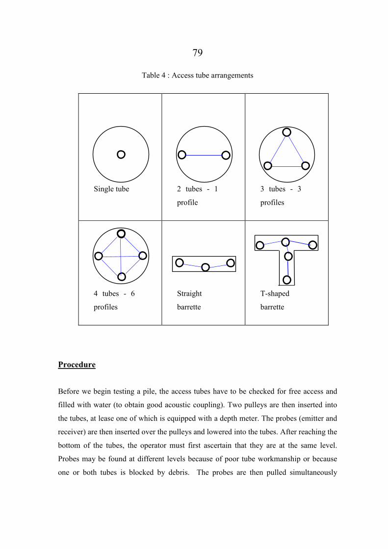
79
Table 4 : Access tube arrangements
Single tube
2 tubes - 1
profile
3 tubes - 3
profiles
4 tubes - 6
profiles
Straight
barrette
T-shaped
barrette
Procedure
Before we begin testing a pile, the access tubes have to be checked for free access and
filled with water (to obtain good acoustic coupling). Two pulleys are then inserted into
the tubes, at lease one of which is equipped with a depth meter. The probes (emitter and
receiver) are then inserted over the pulleys and lowered into the tubes. After reaching the
bottom of the tubes, the operator must first ascertain that they are at the same level.
Probes may be found at different levels because of poor tube workmanship or because
one or both tubes is blocked by debris. The probes are then pulled simultaneously

80
upwards with smooth motion until they reach the pulleys. During this time the emitter
produces a continuous series of pulses, sending waves in all directions. The vertical
distance between successive pulses is determined by the operator, with 50 mm. being a
good typical figure.
Some of these wave paths do eventually reach the receiver. The pulses arriving at the
receiver are recorded and processed by the testing instrument. The operator may then see
the results on the screen.
Presentation of the results
According to the French Standard (AFNOR 2000), the test report should, as a minimum,
present for each pile full identification details: the project description, job number, date,
pile number and tube arrangement. For each profile in the pile the first arrival time
(FAT) of each pulse versus depth should be plotted (a). Later standards (ASTM 2008)
demand, in addition, a plot of the relative energy versus depth. For this purpose, the
energy carried by each pulse is defined as that area enclosed between the pulse envelope
and the horizontal axis. The energy units are typically mVµsec. If the maximum possible
energy is takes as reference, the fraction of this value calculated for each pulse is defined
as the relative energy. Since energy may vary over two or three orders of magnitude, the
scale for relative energy is usually logarithmic (c). ASTM (2008) also requires the
presentation of a “waterfall” representation. This form is obtained by transforming each
pulse into a narrow band. The highest peaks of the pulse are shown in black and the
deepest troughs by white. Intermediate values are shown as gray scale. All the bands are
then stacked together, giving an overview of the whole profile (f). In addition to the
above plots modern instruments, such as the CHUM, are capable of showing the
following:
Apparent velocity versus depth (b) - obtained by dividing the tube spacing by the FAT.
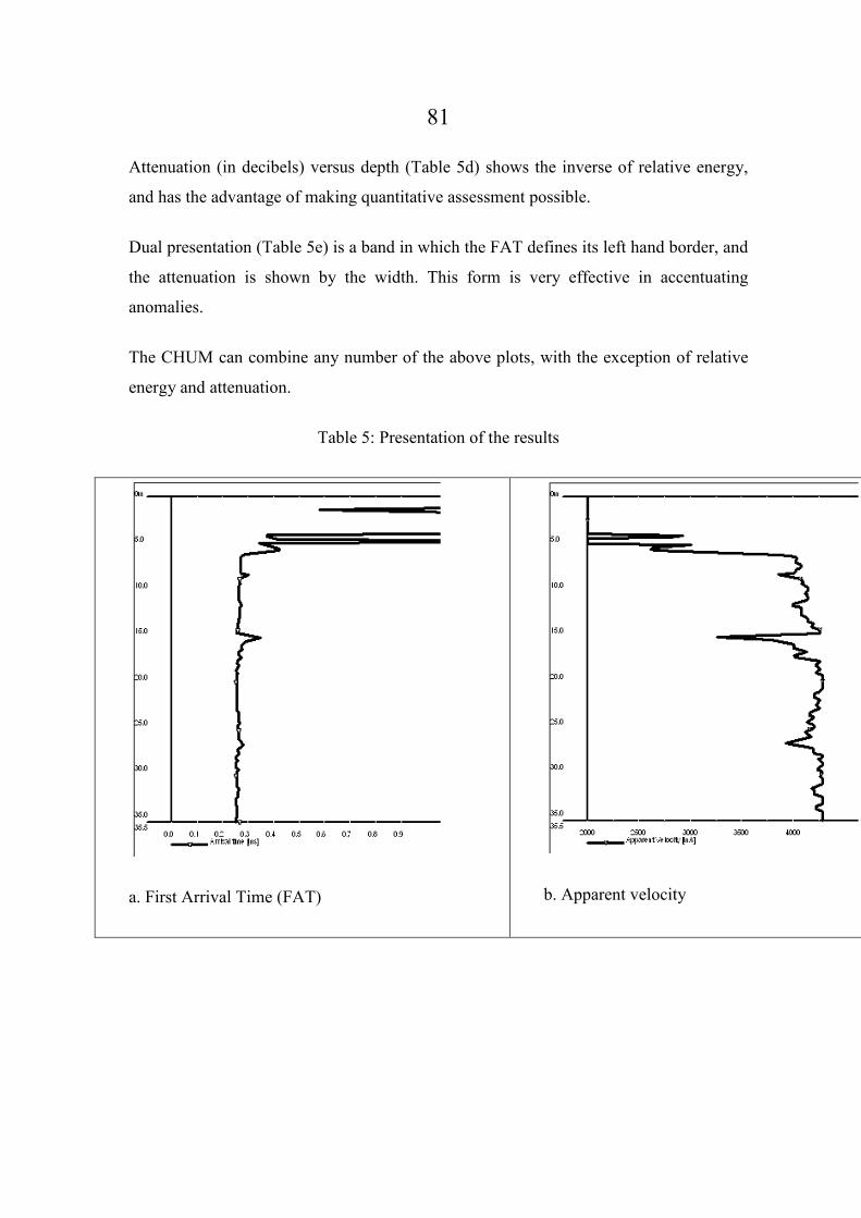
81
Attenuation (in decibels) versus depth (Table 5d) shows the inverse of relative energy,
and has the advantage of making quantitative assessment possible.
Dual presentation (Table 5e) is a band in which the FAT defines its left hand border, and
the attenuation is shown by the width. This form is very effective in accentuating
anomalies.
The CHUM can combine any number of the above plots, with the exception of relative
energy and attenuation.
Table 5: Presentation of the results
a. First Arrival Time (FAT) b. Apparent velocity

82
c. Relative energy (no scale)
d. Attenuation (dB)

83
e. Dual presentation
f. Waterfall presentation
Interpretation
While any good technician can successfully carry out a cross hole test, the interpretation
of the results should be left to experienced geotechnical engineers. The two main
parameters that have to be considered when looking at the test results are the FAT and
the measured energy.
First arrival time (FAT)
The first item is the shape of the FAT vs. depth plot. As long as FAT is more or less
constant, it indicates that there is no change in concrete quality between the tubes along
the pile. A local increase of the arrival time is considered as an anomaly that may be the
result of an obstacle (or flaw) on the straight path between the probes at the

84
corresponding depth. The ultrasonic waves will either travel through this flaw at a
reduced velocity or bypass it, with a respective increase in travel time.
Experimental work (Stain & Williams 1991) indicated that lower-strength concrete has
little effect on either transmission time or signal attenuation. On the other hand,
segregated (honeycombed) concrete, bentonite-polluted concrete and pockets of pure
bentonite slurry do strongly affect the signal.
FAT picking by sight for every pulse is fairly straightforward. But when dealing with
thousands of pulses, as is the case in a typical pile, it becomes an impractical
proposition. We have therefore to use some automatic process, or suitable algorithm, to
perform this task for us. We have at our disposal several methods designed exactly for
this purpose:
Fixed threshold
In this method, we tacitly assume that the first arrival time occurs when the signal
strength first exceeds a predetermined signal level, or threshold. Since this can give
erroneous results in noisy pulses, the refined version of this method allows the operator
to dictate a lower-bound value for the FAT, depending on the probe separation. The
fixed threshold method is very simple, but may give us totally wrong answers in weak
signals (Figure 29).
Figure 29: FAT picking by fixed threshold in strong (left – 10V scale) and weak signal
(right – 1V scale)

85
Dynamic threshold
The dynamic threshold overcomes the main drawback of the fixed threshold method, by
assigning to each pulse a different threshold, which is a fraction of the maximum
amplitude. Thus for a strong signal we have a high threshold, and for a weak signal a
correspondingly low threshold. A good choice of the fraction is crucial to the success of
this method.
Moving windows (STA/LTA)
This method uses a long moving window in which a short window is included in the
right hand side (Figure 30). As both windows are shifted from the origin to the right,
pixel by pixel, the ratio between their respective average amplitudes (STA/LTA) is
constantly calculated. The FAT is set at the point where the ratio exceed a predetermined
value,
Figure 30: The moving windows FAT picking method

86
Automatic FAT picking
This iterative algorithm assumes that the FAT is located between the origin and the
maximum pulse amplitude V0. To start with, the program plots the pulse envelope, and
the time in which the maximum point occurs is defined as T0. The algorithm then
performs the following tasks (Figure 31):
1. A diagonal is drawn from (0,V0) to (T0,0).
2. The point where this diagonal first crosses the envelope is (T1,V1)
3. A diagonal is drawn from (0,V1) to (T1,0).
4. Steps 2 and 3 are repeated until Tn+1 = Tn, which is then defined as the FAT.
The major advantage of this method is that, unlike all others, it requires no arbitrary
parameters.
Figure 31: Automatic FAT picking

87
Accuracy
England (1995) itemized the factors that influence the accuracy of the test in terms of
arrival time. Among these are:
1. Free movement of the probes within tubes of larger diameter
2. Probes not being at the same level
3. Tubes not exactly parallel
4. Air gap or different material around the tube
5. Measurement resolution
According to England, the accumulated error due to all these factors may amount to 20
percent. He therefore suggests that only larger variations should justify further
investigation.
To the above factors, Amir et al. (2004) also added the normal scatter of concrete
strength and the FAT picking error. As a result of all this, they estimated that the total
error may reach 10% of the FAT value plus 27 µsec. The effect of this error is very
marked when the tubes are closely-spaced.
From the above, it is obvious that for a given pulse, FAT is not a unique value, as it
depends strongly on the algorithm used and, within that algorithm, on the parameters
selected. Figure 32 amply proves this point. Moreover, experience has shown that no
single algorithm will give satisfactory results for all types of pulses. FAT picking is,
therefore, a process which calls for careful judgment. Deciding which method is
preferable is sometimes difficult, and at present the best standard against which a
particular method can be judged is the visual method.

88
a. Low threshold
b. High threshold
Figure 32: Influence of the fixed threshold on the FAT obtained
Energy
Energy is the other useful parameter which we obtain from the ultrasonic test. It is true
that in uniform concrete the both energy and FAT depend on the distance traveled Figure
22, but still it pays to study them separately. The main reason for this is that, unlike
FAT, which can assume many values, energy is practically invariant.
If the waves pass through an inclusion, both parameters should be affected. A local
increase in FAT without a corresponding decrease in energy may mean that we are using
the wrong FAT picking method. If, on the other hand we notice a decrease of the
measured energy without an increase in FAT, it usually is a result of a constriction of the
travel path and the defect is located out of the straight line connecting the probes
(Figure 33).

89
Figure 33: Location of defects in a pile
Special techniques
Tomography
When a flaw is located in a certain region of the pile the test may be repeated, but this
time with the probes at different levels (Figure 34). This technique, borrowed from
medicine, is called tomography and it enables us to define both the location and size of
the inclusion.
Figure 34: Ultrasonic tomography
To perform pile tomography, we start the test normally, pulling both probes
simultaneously upward. When an anomaly is encountered, we procedd as follows:
1. Pulling is stopped about one meter above the anomaly.
2. One of the probes (let's call it A) is lowered until the signal becomes very weak.
3. The second probe (let's call it B) is lowered a little (say 100 mm) and probe A raised until
the signal is almost lost.

90
4. Probe B is further lowered in stages, and probe A alternately lowered and raised until the
signal is lost.
5. The procedure is repeated until the anomaly is fully formed on the screen.
6. The probes are brought to the same level, and the test continued in the normal fashion all the
way to the top.
The above technique produces horizontal readings, as well as reading inclined both
ways. To analyze the problem, the zone tested is arbitrarily divided into a grid of small
elements called pixels and the FAT is then calculated for all rays passing through the
zone. At this point, we can choose among three analytical approaches:
Simultaneous equations
If we define the inverse of wave speed as slowness s = 1/c, the arrival time for a ray i is:
jiji sLt Σ= Equation 29
where Lij is the distance traveled by ray i in pixel j, and sj is the slowness of pixel j. if the
pixels are small enough, all Lij values can be replaced by 1 with little effect on accuracy.
Since the number of measurements usually exceeds the number of pixels, the resulting
system of equations is overdetermined, and can be solved with suitable mathematical
techniques (Bowen & Dianguang 1992). The resulting slowness values can then be
converted into wave speeds and plotted in contour form. As we have already seen, the
wave speeds can correlated with concrete quality.
The same procedure, which is carried out in two dimensions on a single profile, can be
used in three dimensions for the whole pile. In this case, the pile is divided into
elementary voxels, or volume pixels. The mathematical treatment is the same. An
important point with 3-dimensional tomography (3DT) is that distances between the
access tubes must be measured very accurately.
The 3DT output can be presented in various forms:

91
1. Using special viewing software enables dynamic presentation with which the user
can rotated the pile, look at it from different angles and zoom in on areas of special
interest (Figure 35).
2. Horizontal and/or vertical cross sections where anomalies are found (Figure 36).
Figure 35: Three-dimensional visualization of pile anomalies
1
2
3
4
0.75m 0.75m00.60m 0.40m 0.20m 0.20m 0.40m 0.60m
Figure 36: Horizontal cross section at 20.4 m

92
In all forms, the user can choose a threshold wave speed which will empasize the
inclusions on the blank background which denotes sound concrete.
Fuzzy logic tomography
The analysis can be simplified, at some sacrifice to accuracy, by using fuzzy logic
techniques (Santamarina 1994). In this approach, every pixel is assigned a quality index
on a scale of 1 to 10. To obtain the quality index, all the rays passing through the region
are scrutinized, and the FAT values of the inclined rays corrected for inclination,
according to the following expression:
22 )( yS
SFATFATcorr
∆+= Equation 30
Where FATcorr is the corrected arrival time, S is the tube spacing and ∆y is the difference
in probe level. The rays with the normal FATcorr in the region are assigned a fuzzy value
of 10 and the ray with the maximum FATcorr – a fuzzy value of 1. The rays between
these boundaries are given intermediate values by interpolation. Since a “good” ray
cannot pass through a “poor” pixel, the quality index of a pixel is equal to the highest
fuzzy value of all the rays passing through it. A suitable map of the pixels will then
show inclusion with inferior material (Figure 37).

93
Figure 37: Result of fuzzy logic tomography (left) and the exposed defect (right)
Parametric tomography
In the parametric approach, we start with two reasonable assumptions:
• At any given level there is only one inclusion.
• The inclusion is in the shape of an upright rectangle.
From the horizontal rays, we know y1 and y2, that is the lower and the upper coordinates
of the rectangle, respectively. To define the rectangle, all we need just two more
parameters – the left hand coordinate xL and the right hand coordinate xR. The procedure
works as follows:
1. We define some rectangle by assuming the values of xL and xR.
2. We take all rays that we logged through the region. For rays passing through the
assumed rectangle, we assign the highest measured value of FAT. Those rays that skip
the rectangle get the normal FAT value of the region.

94
3. For every ray, we find the difference ∆t between the measured and the asumed FAT.
4. The sum of the squares of the differecnces Σ(∆t)2 is defined as the residual of the
assumed rectangle.
5. The procedure is repeated for a large number of rectangles, with xL and xR varied
between 0 and S. That rectangle with the lowest residual is considered the best
representation of the inclusion.
Attenuation-based tomography
Up to this point, we presented the classical approach, that of FAT-based tomography.
Since a given inclusion may have a stronger influence on the energy than on the FAT,
attenuation-base tomography may sometimes produce superior results (Amir & Amir
2009). One of the advantages of this approach is that energy, unlike FAT, is practically
invariant. Incidentallly, attenuation, like FAT, is linearly-dependen to distance. The
exact function can be derived from Figure 22or from actual measurements made on a
defect-free zone of the pile.
Tomography can also be based on either/and combination of FAT and energy, and
experience has shown that this is a very promising approach.
Evaluation
Tomography provides us with a two-dimensional pricture of the profuile we are
interested in, and thus can be a powerful technique. Nevertheless, it has a few inherent
shortcomings:
• The method fails close to either the upper or the lower ends of the pile (Figure 38)
• Since we have only a limited range of viewing angles (none close to vertical), we shall
always get shadows that will extend the defects horizontally (Figure 39).
• The solution is not necessarily unique, and in certain cases may yield erroneous results
(Santamarina 1994).
.........

95
Figure 38: Tomography near the toe - "blind" zone
Figure 39: Stages in real-time fuzzy-logic tomography
1. The real inclusion
2. Horizontal measurements determinates the vertical coordinates y1 and y2
3. Adding inclined (/) measurements reveals the location of the defect

96
4. Reverse inclined (\) measurements refine the defect shape (note unavoidable
“shadow” areas)
Single-hole testing
Single hole ultrasonic testing (Figure 40) is a variation on the conventional cross hole method. It
is extremely useful under the following conditions:
1. If cross hole testing was planned, but some tubes were accidentally damaged, and only
one is available for testing
2. in piles without tubes where core drilling was performed
3. in hollow driven piles
4. in small diameter piles where there it is impractical to install multiple piles and the sonic
test is inapplicable
Transmitter
Receiver
Signal Path
Defect
Figure 40: Single hole testing
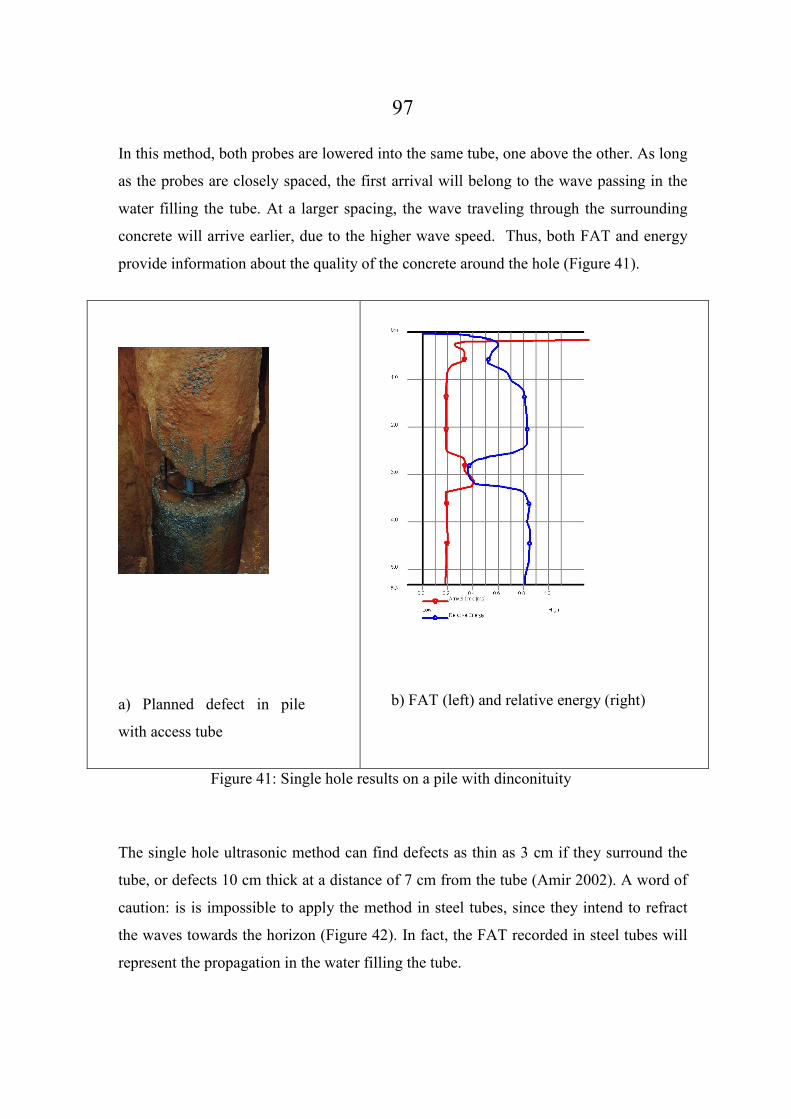
97
In this method, both probes are lowered into the same tube, one above the other. As long
as the probes are closely spaced, the first arrival will belong to the wave passing in the
water filling the tube. At a larger spacing, the wave traveling through the surrounding
concrete will arrive earlier, due to the higher wave speed. Thus, both FAT and energy
provide information about the quality of the concrete around the hole (Figure 41).
a) Planned defect in pile
with access tube
b) FAT (left) and relative energy (right)
Figure 41: Single hole results on a pile with dinconituity
The single hole ultrasonic method can find defects as thin as 3 cm if they surround the
tube, or defects 10 cm thick at a distance of 7 cm from the tube (Amir 2002). A word of
caution: is is impossible to apply the method in steel tubes, since they intend to refract
the waves towards the horizon (Figure 42). In fact, the FAT recorded in steel tubes will
represent the propagation in the water filling the tube.

98
Figure 42: Wave propagation through a PVC tube (left) and a steel tube (right)
Sample Specifications
1. Introduction: For ultrasonic testing, at least two access tubes are cast in the pile. An
ultrasonic transmitter is lowered in one of the tubes and a receiver - in the other. Both
transducers are connected to a computer that plots the time of first arrival FAT, as well
as the energy, versus depth. As long as FAT and energy are approximately constant, the
pile is considered acceptable. A local anomaly, in the form of late arrival or decreased
energy, may mean that the concrete between the tubes is defective at this level. Installing
a larger number of piles along the perimeter of the piles will provide almost complete
coverage of the cross-section.

99
2. Testing agency: The ultrasonic test shall be carried out by a firm experienced in this kind
of work and approved by the Engineer. Both site work and interpretation of the results
shall be carried out by a Geotechnical engineer with proven experience.
3. Equipment: The test shall be performed using a computerized system of reputable origin.
All components shall be recently calibrated and in good working order. All software
shall be of the latest released version.
4. Piles to be tested: All piles shall be tested at a minimum age of Seven days after casting,
unless instructions to the contrary shall be given by The Engineer.
5. Access tubes: All tubes shall be new, straight and clean both inside and outside, with a
minimum internal diameter of 50 mm. All connections shall be welded or glued
externally, taking care that no welding material penetrates inside. Both ends of the tube
shall be tightly plugged. The Contractor shall take all due care to avoid any damage to
the tubes during manufacturing, installation, concreting and the trimming of the head.
6. Preparation for testing: Before commencing the test, the Contractor shall ensure that
there is adequate access to the pile. The Contractor shall use a suitable saw to cut the top
of the access tubes cleanly at a level of 200 to 300 mm above the concrete, unless
ordered otherwise. The tubes shall then be tested for access throughout their length using
a 1” tube as a dummy. Having passed this test, the tubes shall be completely filled with
water.
7. Reporting: A final report for each testing stage shall be presented not later than three
working days after completion of that stage. The report shall consist of a printout of the
original output, as well a summary table including, for every pile tested, the depth and
The Engineers' interpretation regarding its integrity.

100
Radioactive integrity testing
Radioactive testing of piles (Preiss & Caiserman 1975) was the first commercially
available method for the integrity testing of piles. In this method, the probe hung by a
cable is lowered into a steel tube prepared in advance. The probe (Figure 43) consists of
the following components:
1. A weak radioactive source (Usually Cesium 137)
2. A lead shield
3. A photon detector (Geiger counter or similar device)
4. Electronic circuitry and computer
Figure 43: Radioactive Probe (Schematic)
The source emits gamma rays (photons) to all directions, and these are backscattered by
the surrounding material. When the rays hit an inclusion with a lower density, a larger
proportion of them is backscattered and trapped by the counter. Thus, the photon count

101
serves as a measure of the average density of the surrounding concrete: A higher count
means lower density, and vice versa.
The instrument can be calibrated to give direct density readings, but here a word of
caution is appropriate: The photon count includes the effect of all the elements
surrounding the counter, including the tube and the water in the tube (If such exists).
Therefore, the instruments should be calibrated separately for each tube diameter and
wall thickness combination and for both wet and dry situations.
Theoretically, there is no limit to the range of gamma ray penetration. The radiation
energy, however, decreases quickly with penetration. For Cesium 137, for instance, it is
halved for every 50 mm penetration into concrete. Therefore, available radioactive pile
testers have a typical range of only 50 to 75 mm around each tube (Davis & Hertlein
1994).
The main drawback of the radioactive method, in addition to the limited range, is the
utilization of dangerous material. The use of radioactive material is regulated in all
civilized countries, and operating such an instrument for pile testing normally requires a
special license.
The main advantages of the radioactive method over stress-wave methods are as follows:
1. It is possible to test the pile a short time after concreting
2. The method is suitable for acceptance of pile grouting, where stress-wave
methods fail.
3. In spite of these advantages, the radioactive method is rapidly losing ground due
to the great progress made in cross-hole ultrasonic testing.

102
References
1. Afnor (2000): NF P 94-160-1, Auscultation d’un element de fondation – Partie 1:
Methode par Transparence, Paris
2. Amir, J.M. & Amir, E.I (2009): Capabilities and Limitations of Cross Hole Ultrasonic
Testing of Piles, Proc IFCEE, Orlando
3. Amir, E.I. & Amir J.M. (2008): Statistical Analysis of a Large Number of PEM Tests on
Piles, Proc. 8th Intl. Conf on Application of Stress Wave Theory to Piling, Lisbon
4. Amir, E.I. & Amir J.M. (2008a): Critical Comparison of Ultrasonic Pile Testing
Standards, Proc. 8th Intl. Conf on Application of Stress Wave Theory to Piling, Lisbon
5. Amir, J.M. (2007): Discussion on “Reliability Evaluation of Cross-Hole Sonic Logging
for Bored Pile Integrity” by D. Q. Li, L. M. Zhang, W. H. Tang, J Geotech Div ASCE, Vol
133 No. 3, pp. 342-343
6. Amir, J.M. (2005): Discussion on “Low Strain Integrity Testing of Piles: Three–
Dimensional Effects” by Y.K. Chow, K.K. Phoon, W.F. Chow and K.Y. Wong, J Geotech
Div ASCE, Vol 131 No. 2
7. Amir, J.M., Amir, E.I. and Felice, C.W (2004): Acceptance Criteria for Bored Piles By
Ultrasonic Testing, Proc. Intl. Conf on Application of Stress Wave Theory to Piling, Kuala
Lumpur
8. Amir, J.M. (2002): Single-Tube Ultrasonic Testing of Pile Integrity, ASCE Deep
Foundation Congress, Vol 1 pp. 836-850, Orlando
9. Amir, J.M. & Fellenius, B.H. (2000): Pile Testing Competitions – A Critical Review, Proc
Intl. Conf on Application of Stress Wave Theory to Piling, pp. 313-317, Sao Paulo
10. Amir, J.M. (1999): Caveat Emptor or a Buyer’s Guide to Integrity Testing, Proc DFI
Annual Conf, Dearborn
11. Amir, E.I & Amir J.M. (1998): Testing Piles with Virtual Instruments, Proc DFI 7th Intl
Conf on Piling and Deep Foundations, Vienna

103
12. Amir, J.M. & Fellenius, B.H (1996): Discussion on “Small strain sonic pile tests - the
need for caution” by K.Y. Wong, Ground Engineering Vol. 29 No.1
13. Amir, E.I & Amir J.M. (1994): Recent Advances in Ultrasonic Pile Testing, Proc. 3rd
Intl Geotechnical Seminar on Deep Foundation On Bored and Auger Piles, Ghent 1998
14. Komornik, A. & Amir, J.M.: Quality Control at Pier NB-2, Proc. 5th Intl. Conf. DFI,
Bruges,
15. Amir J.M. (1988): Wave speed in young concrete, Proc 3rd Intl Conf on Application of
stress-wave theory to piles, Ottawa
16. Amir J.M. (1983): Discussion on "Shaft integrity by wave propagation method" by T.M.
Hearne Jr. & K.H. Stokoe, J Geotech Div ASCE No. GT12
17. ASTM (2007): Standard test method for low strain integrity testing of piles, Designation
D5882-07, Philadelphia PA
18. ASTM (2008): Standard test method for integrity testing of concrete deep foundations by
ultrasonic crosshole testing, Designation D6760-08, Philadelphia PA
19. Bilancia, R., Caputo, V. & DiMuro, E.(1996): Some experiences of low strain tests on
piles of known geometry, Proc. 5th Intl. Conf. Application of Stress Waves to Piles,
Orlando, pp. 831-845
20. Bowen, H. & Dianguang, W. (1992): Application of sonic tomography in the integrity
testing of concrete piles, Proc. 4th Conf. Application of Stress Waves to Piles, Rotterdam, pp.
231-234
21. Brettmann, T. & Frank, M. (1976): Comparison of crosshole and single hole sonic
integrity logging methods, Proc. 5th Intl. Conf. Application of Stress Waves to Piles,
Orlando, pp. 698-707
22. Danziger, B.R., Lopes, F.R., Costa, A.M. & Pacheco, M. P. (1976): A discussion on the
uniqueness of CAPWAP-type analyses, Proc. 5th Intl. Conf. Application of Stress Waves to
Piles, Orlando, pp. 394-408
23. Davis, A.G. & Hertlein, B.H. (1994): A comparison of the efficiency of drilled-shaft
down-hole integrity tests, Proc. FHWA Intl. Conf. On Design and Construction of Deep
Foundations, Orlando

104
24. De Jaeger, J, Carpentier, R. & van den Broek, M. (1987): Ch IV - Essais d’Integrite,
Seminar On Pile Dynamic Testing Integrity And Bearing Capacity, Brussels, pp. 1-62
25. Ellway (1993): Objectives of competition are unclear, Ground Engineering, June p. 8
26. England, M. (1995): Private communication quoted in CIRIA Funders Report CP/28 on
the role of integrity and other non-destructive testing in the evaluation of piled foundations
27. Fleming, W.G.K., Weltman, A.J., Randolph, M.F. & Elson, W.K. (1992): Piling
Engineering, Blackie A & P, Glasgow (2nd ed.)
28. Fukuhara, T., Kakurai, M. & Sugimoto, M. (1992): Analytical evaluation of defective
piles, Proc. 4th Conf. Application of Stress Waves to Piles, The Hague, pp. 563-569
29. Graff, K.G. (1975) : Wave motion in elastic solids, Clarendon Press, Oxford
30. ICE (1996): Specification for piling and embedded retaining walls, London
31. Klingmuller, O. (1992): Pile integrity testing as a problem of on site quality control,
Proc. 4th Conf. Application of Stress Waves to Piles, The Hague, pp. 577-580
32. Kolsky, H. (1963): Stress waves in solids, Dover Publications, New York
33. Komornik, A. & Amir, J.M.: Quality Control at Pier NB-2, Proc. 5th Intl. Conf. DFI,
Bruges, 1994
34. Plassmann, B. (2002): Zur optimierung der messtechnik und der auswertenmethodik bey
pfahlintegritatsprufungen, Mitt. Inst. Grundbau und Bodenmechanik, TU Braunschweig
35. Rausche, F., Likins, G.E. & Hussein, M (1988): Pile integrity testing by low and high
strain impacts, Proc. 3rd Conf. Application of Stress Waves to Piles, Ottawa, pp. 44-55.
36. Rausche, F., Likins, G.E. & Kung, S.R.: (1992): Pile integrity testing and analysis, Proc.
4rd Conf. Application of Stress Waves to Piles, The Hague, pp. 613-617.
37. Reiding, F.J. (1992): Computer-integrated pile test equipment, Proc. 4th Conf.
Application of Stress Waves to Piles, The Hague, pp. 313
38. Samman, M.M. & O’Neill, M.W. (1997): An exercise in seismic testing of drilled shafts
for structural defects, Foundation Drilling, January, pp. 11-17
39. Santamarina, J.C. (1994): An introduction to geotomography, Geophysical
characterization of sites (R.D. Woods, ed.), Balkema, Rotterdam, pp. 35-43
40. Santamarina, J.C., Klein, K.A. & Fam, M.A. (2001): Soils and Waves, Wiley, Chi
Chester

105
41. Sliwinski, Z.J. & Fleming, W.G.K. (1983): the integrity and performance of bored piles,
Proc. Int. Conf on Piling and Ground Treatment, London, pp. 211-223
42. Smits, M.Th.J.H. (1996): Pile integrity tests, Proc. 4th Conf. Application of Stress
Waves to Piles, The Hague, Vol. II pp.25-54
43. Stain, R (1993): Test’s integrity is questionable, Ground Engineering January/February,
p. 7
44. Stain, R (1993a): Competition was not applicable, Ground Engineering, April p. 15
45. Stain. R.T. & Williams, H.T. (1991): Interpretation of sonic coring results: A research
project, Proc. 4th Intl. Conf. Piling & Deep Foundations, Stresa, pp. 633-640
46. Steinbach, J. & Vey, E. (1975): Caisson valuation by stress-wave propagation method,
.J. Geotech. Div. ASCE, Vol 101 No. GT4, April
47. Task force (2000): Nondestructive evaluation of drilled shafts, J. Geotechnical and
Geoenvironmental Engineering ASCE, January, pp. 92-95
48. Turner, M.J. (1997): Integrity testing in piling practice, CIRIA. London
49. Vyncke, J. & van Nieuwenburg, D.(1987): Ch. II - Theorie van de dynamische proeven:
A. Integriteint, Seminar On Pile Dynamic Testing Integrity And Bearing Capacity, Brussels,
pp. 1-49