1

Development of Biological Indicators and Targets to Guide Sediment TMDLs for Streams of the Central Coast Region of California and the San Lorenzo River

Final Report January 2011

Contract 07-125-130

David B. Herbst, R. Bruce Medhurst and Scott W. Roberts

Sierra Nevada Aquatic Research Laboratory University of California

and Jonathan W. Moore

Dept Ecology and Evolutionary Biology UC Santa Cruz

Table of Contents

1. Introduction And Overview ........................................................................................... 1

2. Physical Habitat and Reference-Test Designations ....................................................... 2

3. Native Salmonids and Non-Native Crayfish in 2009 Surveys..................................... 11

4. Macroinvertebrate Community Metrics and Sediment Deposition ............................. 14

Summary and Conclusions…………………………………………………...….22

Maps.................................................................................................................................. 25

Appendix (stream site indicators & impairment listings)………………………………..28 Main Findings:

� At a threshold in the range of 30-40% fine and sand (FS) sediment cover,

there is substantial loss of biological diversity of invertebrates

� Along with changes in selected biological indicators, this level of FS sediment

cover can be used as numeric criteria for sediment impairment

� Where biological indicator metrics fall below the 25th percentiles of their

reference stream levels, biological criteria can be set for impaired condition

� Rainbow trout abundance is reduced above 6% fine substrate cover, so this

may be used a separate criterion for steelhead streams

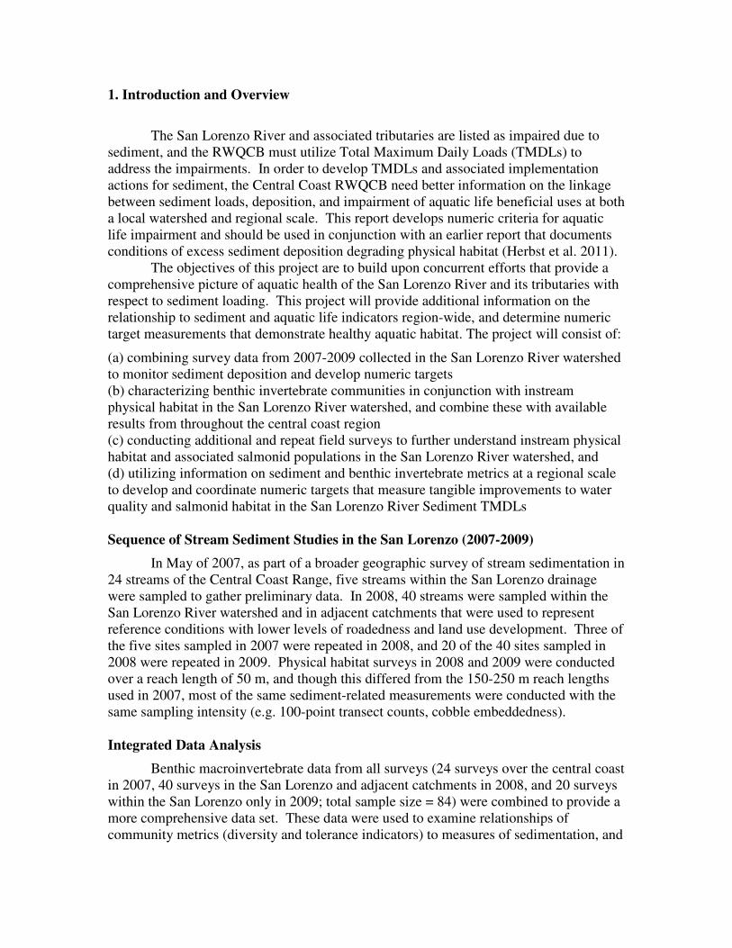
1. Introduction and Overview

The San Lorenzo River and associated tributaries are listed as impaired due to

sediment, and the RWQCB must utilize Total Maximum Daily Loads (TMDLs) to address the impairments. In order to develop TMDLs and associated implementation actions for sediment, the Central Coast RWQCB need better information on the linkage between sediment loads, deposition, and impairment of aquatic life beneficial uses at both a local watershed and regional scale. This report develops numeric criteria for aquatic life impairment and should be used in conjunction with an earlier report that documents conditions of excess sediment deposition degrading physical habitat (Herbst et al. 2011).

The objectives of this project are to build upon concurrent efforts that provide a comprehensive picture of aquatic health of the San Lorenzo River and its tributaries with respect to sediment loading. This project will provide additional information on the relationship to sediment and aquatic life indicators region-wide, and determine numeric target measurements that demonstrate healthy aquatic habitat. The project will consist of:

(a) combining survey data from 2007-2009 collected in the San Lorenzo River watershed to monitor sediment deposition and develop numeric targets (b) characterizing benthic invertebrate communities in conjunction with instream physical habitat in the San Lorenzo River watershed, and combine these with available results from throughout the central coast region (c) conducting additional and repeat field surveys to further understand instream physical habitat and associated salmonid populations in the San Lorenzo River watershed, and (d) utilizing information on sediment and benthic invertebrate metrics at a regional scale to develop and coordinate numeric targets that measure tangible improvements to water quality and salmonid habitat in the San Lorenzo River Sediment TMDLs Sequence of Stream Sediment Studies in the San Lorenzo (2007-2009)

In May of 2007, as part of a broader geographic survey of stream sedimentation in 24 streams of the Central Coast Range, five streams within the San Lorenzo drainage were sampled to gather preliminary data. In 2008, 40 streams were sampled within the San Lorenzo River watershed and in adjacent catchments that were used to represent reference conditions with lower levels of roadedness and land use development. Three of the five sites sampled in 2007 were repeated in 2008, and 20 of the 40 sites sampled in 2008 were repeated in 2009. Physical habitat surveys in 2008 and 2009 were conducted over a reach length of 50 m, and though this differed from the 150-250 m reach lengths used in 2007, most of the same sediment-related measurements were conducted with the same sampling intensity (e.g. 100-point transect counts, cobble embeddedness). Integrated Data Analysis

Benthic macroinvertebrate data from all surveys (24 surveys over the central coast in 2007, 40 surveys in the San Lorenzo and adjacent catchments in 2008, and 20 surveys within the San Lorenzo only in 2009; total sample size = 84) were combined to provide a more comprehensive data set. These data were used to examine relationships of community metrics (diversity and tolerance indicators) to measures of sedimentation, and

2

community ordination was used to evaluate similarity among sites in overall biological response to environmental gradients of sediment and other habitat variables.

The combined data set was also used to document different physical habitat measures of sedimentation contrasting reference and test streams for the population of 84 combined surveys. As described in the more detailed report on sediment loads, deposition, and land use, the upper quartile of the reference range of stream sediment deposition was use to define impairment thresholds (Herbst et al. 2011).

In addition to habitat and macroinvertebrate data, surveys of anadromous rainbow trout (steelhead, Oncorhynchus mykiss) and crayfish (Pacifastacus leniusculus) were conducted in June of 2009 at 20 sites in the San Lorenzo River drainage (repeats of 2008 study sites). At these sites we also collected non-native crayfish, and in this way, we incorporate multiple biological indicators and key species that may be affected by the varied levels of sedimentation found. 2. Physical Habitat Survey Methods (2008-2009) and Reference-Test Designations

Surveys of the physical habitat of each study site emphasized measures of sediment deposition taken concurrent with benthic invertebrate samples in order to link both habitat and biological response variables to the land use and sediment loading of each catchment. Methods for documenting physical habitat characteristics differed between the 2007 sediment TMDL surveys, and San Lorenzo surveys in 2008 and 2009. These methods are outlined below (refer also to Herbst et al. 2011 sediment report).

• Study reaches were 50 meters in length (San Lorenzo 2008 and 2009); 150 meters in length for streams with an average width of less than 10 m, or 250 meters in length for streams wider than 10 meters (sediment TMDL 2007).

• We measured substrate particle size distribution along cross-sectional transects spaced over the entire study reach. For San Lorenzo 2008 and 2009: 10 transects at 10 points, for the sediment TMDL project of 2007: 20 transects at 5 points. Substrate size was measured as the intermediate axis of all particles larger than 2 mm, or recorded as sand for particles estimated as 0.25 to 2 mm, or as fines if < 0.25 mm (surveyors were trained to recognize these classes by texture).

• When cobble substrates (64 – 256 mm in diameter) were encountered at sample points, embeddedness was measured as the percentage (±5%) of the stone volume embedded/buried in sand and or fine substrate. Group training of observers was conducted prior to surveys to achieve consistent scoring of embeddedness. If 25 embeddedness measurements were not recorded on completion of transects, remaining counts were obtained from random locations throughout the reach.

• At ten transects, we measured cross-sectional width and depth to determine bankfull channel dimensions. For 2007 sites, we recorded twenty evenly-spaced depth (height) measurements as the distance from the stream bed to a taught meter tape stretched between bankfull marks on both banks. For San Lorenzo 2008 and 2009 sites, we measured bankfull height from the water surface to the bankfull level. Depth of water measurements were taken at ten evenly-spaced points along each transect. In the case of dry points, the measurement was marked as dry. For the wetted locations, the final bankfull depth was simply the water depth plus the

3

bankfull height above water. For the dry locations, we had to make assumptions about the channel profile. For dry locations that were on the edges of the transect, we assumed that the channel elevation profile followed a linear path between the last wetted point and the bankfull elevation. Dry locations that were between wetted points were assumed to be relatively close to the water surface, and we assigned the water surface elevation to these points.

• In addition to these sediment deposition measures, we also measured depth profiles across all transects; channel slope; bankfull channel width; and temperature, conductivity and pH (Oakton con10 meter). Photographs were taken from the middle of the channel, looking downstream and upstream, at fifty meter intervals. GPS coordinates were recorded to provide a georeference point for each study reach.

For San Lorenzo 2008 and 2009 only: • In order to generate high-resolution data on fine particle distribution at the patch-

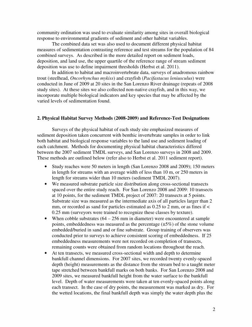
scale within each study reach, we used a grid-frame to measure separate counts of fine and sand particles at twenty-five intersecting grid line points of the grid-frame (Figures 1 and 2) at twenty different locations within the study reach, for a total of 500 point-counts in each study reach. These twenty locations included eleven locations (corresponding to the macroinvertebrate sample locations) at alternating combinations of left-center-right longitudinal positions starting at the beginning of the reach, at zero meters, and at every five meters until the end of the reach, at 50 meters. Nine additional grid counts of fines and sand were positioned offset and upstream of these other eleven locations (Figure 1).

• We drew stream bed facies maps depicting the distribution and composition of contiguous large patches of substrates within the fifty meter reach. These maps were drawn on grid paper scaled to the width and length of each study reach. Fines and sand facies were used to express sedimentation. Gravel facies may be used as an indicator of potential area available for salmonid spawning (redds). Facies can be defined as discrete deposits of bed-surface sediments or rock of uniform grain size where most of the material is comprised of a single class (fines, sand, gravel, pebble, cobble, boulder).

Physical Habitat Analysis

The first category of measures are standard geomorphic measurements taken during pebble counts, including percent sands and fines, percent sands, fines, and gravel, D50 median grain size, and embeddedness. The second category, for the San Lorenzo 2008 and 2009 sites, is taken from the grid sampling and facies mapping procedures, and includes the percent of sands and fines coverage measured at random grid sample sites and the percent of sand and fines visually estimated by facies mapping. A third category, relative bed stability involves comparing the difference between the expected particle size distributions (based on theory of stream power effects on particles) and those particles observed (usually expressed as the median particle size or D50).

Our methodology for calculating Relative Bed Stability (RBS) was taken from the Environment Protection Agency methodology (Kaufmann et al 1999) that has been used

4

for the western EMAP rivers and streams assessment (Stoddard et al. 2005). These measures calculate the departure of substrate conditions from what is the expected condition, based on reach slope and geometry. The equation for Relative Bed Stability is:

RBS = [D50] / [13.7 * Rbf * S], where D50 is the median grain size (mm), Rbf is the mean reach hydraulic radius, and S is reach slope.

Figure 1. Transects for determination of particle size distribution and embeddedness, bed facies maps, and locations of grid counts of fines/sand (and invertebrate sample points). This is the systematic lay-out for stream surveys conducted in 2008 and 2009 for the San Lorenzo and adjacent watersheds of the region (see maps section at end of report for locations).

10 transects at 10 point-intercepts each 5 meter intervals

Bed facies map

gravel

fines

sand

11 reach-wide multi-habitat sample points

9 off-set grid count frames

0 meters

50 meters

50-meter length study reach: Incorporates mixed habitat (flow and morphology)

5

Figure 2. Quadrat grid-frame for particle counting of substrate composition (upper) and with D-frame net positioned for sampling benthic macroinvertebrates (lower).

6

Reference-Test Designations

We partitioned sites into reference and test groups based on their exposure to human-related sources of sediment input. These were identified from breaks or discontinuities in site distribution for co-plots of road density and human land use within the catchment. We derived road locations from Topologically Integrated Geographic Encoding and Referencing (TIGER) dataset produced by the U.S. Census Bureau. We calculated road density as the length of road within a one hundred meter riparian buffer divided by the area of the one hundred meter riparian buffer (km/km2). Road crossings were calculated as the number of road-stream intersections in a watershed divided by the total length of stream segments in a watershed (road crossings/km). We derived human land use from the 2001 National Land Cover Dataset (NLCD). NLCD 2001 provides a classification of land surfaces from 2001 Landsat 7 satellite data (Appendix A). We defined human influence cover as all NLCD classes that are the result of human-related activities. These include 21 (developed, open space), 22 (developed, low intensity), 23 (developed medium intensity), 24 (developed high intensity), 71 (grassland/herbaceous), 81 (pasture/hay), and 82 (cultivated crops). We calculated the percentage of surface cover of these classes within each catchment.

For the Central Coast Range sites surveyed in 2007, we designated reference sites as having �3.0 km/km2 riparian road density and �10% combined human land uses within the watershed (Figure3). Some reference exclusions were made based on local disturbances not evident in GIS. Through our selection process, we identified 14 reference sites and 10 test sites in the Central Coast Range. For San Lorenzo sites surveyed in 2008 and 2009, we also designated references as having �3.0 km/km2 of riparian road density and �10% combined human land uses within the watershed (Figure 4), partitioning 19 reference and 21 test sites. Reference sampling was repeated at 6 sites in 2009, bringing the total reference site surveys to 39.

0

5

10

15

20

25

0 1 2 3 4 5 6

Riparian Road Density (km/km2)

Cat

chm

ent %

Hum

an L

and

Use

reference sites(with exclusionsas open symbols)

Figure 3. Partition of reference site data set for the Central Coast Range sites surveyed in 2007 based on low levels of riparian road disturbance (�3 km/km2) and combined human land use �10%. [specific exclusions (open symbols) based on local disturbances present]

7

0.0

1.0

2.0

3.0

4.0

5.0

6.0

7.0

0% 10% 20% 30% 40% 50% 60%

Human Disturbance (% of catchment)

Rip

aria

n R

oade

dnes

s (k

m/k

m2 )

Reference Sites

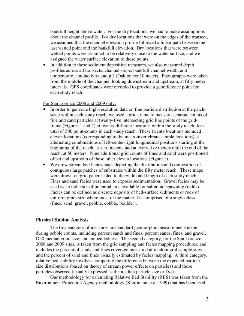
Figure 4. Partitioning of reference and test sites for the San Lorenzo sites surveyed in 2008 and 2009 based on discontinuity in plot of human disturbance measures. References represents least-disturbed state for this population of study sites (�10% human influence, and �3 km /km2 roads in riparian area). Differences Between Reference and Test Sites

• We found differences in instream physical habitat measures between reference and test sites. All contrasts and statistical differences were consistent with our expectations for the response of channel geomorphology and sediment storage to increased landscape disturbance. The test sites, with greater levels of road and land use disturbance, contained more deposition of sediment.

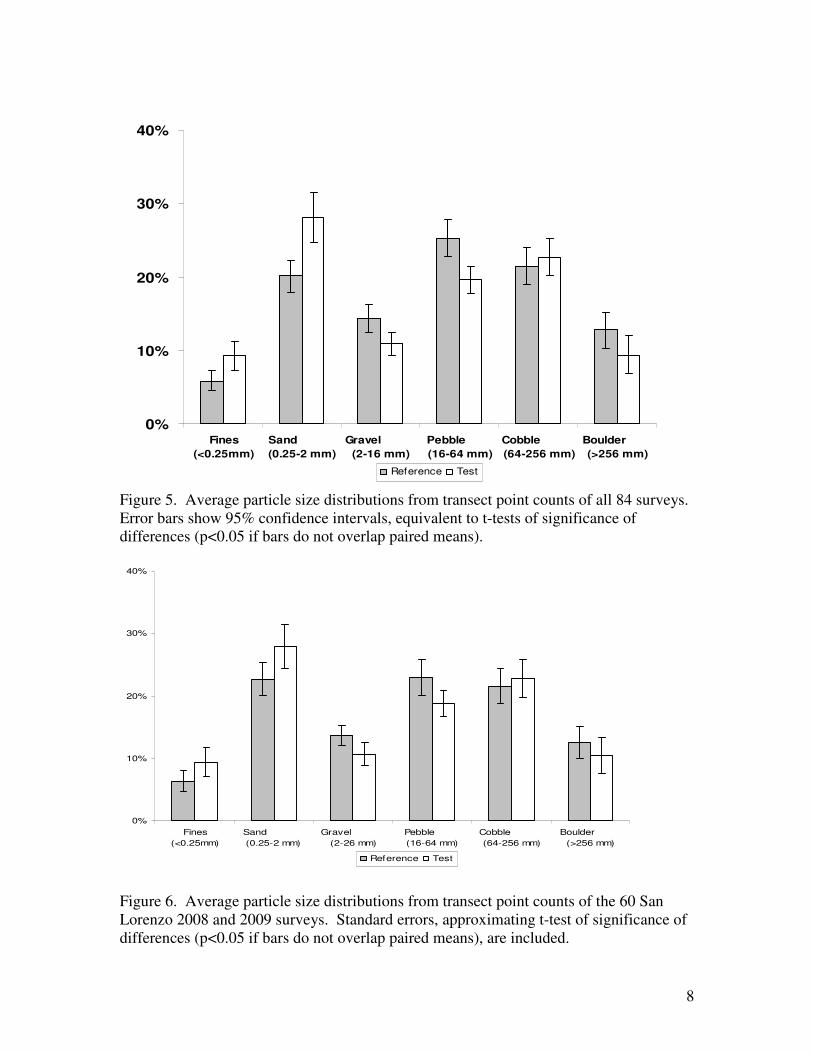
• On average, reference sites had lower percentages of fines and sand and higher

percentages of pebble, cobble and boulder than test sites, whether considered as all surveys combined (Figure 5), or the San Lorenzo and adjacent drainages only (Figure 6). Reference sites had significantly less fine and sand cover measured at the reach scale in point transects (Figure 7) as well as at the patch scale in grid quadrats (Figure 8).

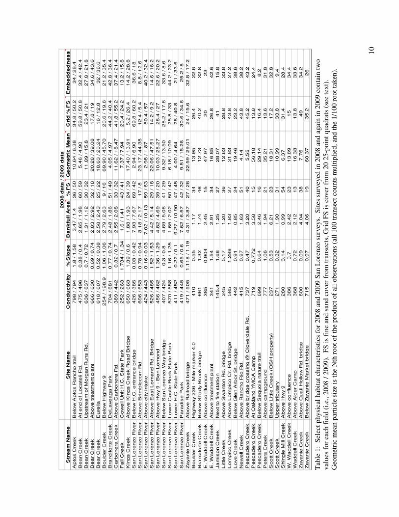
• Measures of habitat, water quality and substrate features were mostly consistent

between years of measurement for those sites where 2008 surveys were repeated in 2009 (Table 1)

8

0%

10%

20%

30%

40%

Fines(<0.25mm)

Sand (0.25-2 mm)

Gravel (2-16 mm)

Pebble (16-64 mm)

Cobble (64-256 mm)

Boulder (>256 mm)

Reference Test

Figure 5. Average particle size distributions from transect point counts of all 84 surveys. Error bars show 95% confidence intervals, equivalent to t-tests of significance of differences (p<0.05 if bars do not overlap paired means).

0%

10%

20%

30%

40%

Fines(<0.25mm)

Sand (0.25-2 mm)

Gravel (2-26 mm)

Pebble (16-64 mm)

Cobble (64-256 mm)

Boulder (>256 mm)

Reference Test

Figure 6. Average particle size distributions from transect point counts of the 60 San Lorenzo 2008 and 2009 surveys. Standard errors, approximating t-test of significance of differences (p<0.05 if bars do not overlap paired means), are included.

9

0%

10%

20%

30%

40%

50%

Reference Test

% F

ines

and S

and

Figure 7. Percent Fines and Sand from transect point counts of all 84 surveys. Standard errors, approximating t-test of significance of differences (p<0.05 if bars do not overlap paired means), are included.

0%

10%

20%

30%

40%

Reference Test

% G

rid F

ines

and S

and

Figure 8. Percent Fines and Sand from grid counts of all 84 surveys. Error bars show 95% confidence intervals, equivalent to t-tests of significance of differences (p<0.05 if bars do not overlap paired means).

10

Str

ea

m N

am

eS

ite N

am

eC

on

du

ctiv

ity

%S

lop

eB

an

kfu

ll A

rea

%F

SG

eo

metr

ic M

ean

Gri

d %

FS

Em

bed

de

dn

es

sA

pto

s C

ree

kB

elo

w A

pto

s R

ancho tra

il79

8 / 7

94

1.8

/ 1

.58

3.4

7 / 1

.436 / 5

010

.64

/ 6

.38

34.8

/ 5

0.2

34

/ 2

8.4

Be

an C

reek

At end

of L

oca

teli

Rd.

47

5 / 4

96

0.3

8 / 0

.42

.65 / 1

.98

60 / 5

95.4

6 / 4

.90

59.8

/ 5

0.8

32

.4 / 4

2.4

Be

an C

reek

Up

str

ea

m o

f M

org

an R

uns R

d.

63

6 / 6

37

0.7

/ 0

.72

1.3

1 / 1

.12

30 / 3

211

.89

/ 1

5.8

23

.4 / 2

127

.8 / 2

1.8

Be

ar C

ree

kA

bove

tre

atm

ent pla

nt

66

6 / 6

30

0.6

9 / 0

.74

2.8

3 / 2

.92

32 / 1

82

0.2

8 / 3

9.0

817

.8 / 1

934

.6 / 4

3.6

Be

ar C

ree

kE

ure

lla61

8 / 6

07

0.5

2 / 0

.38

2.5

8 / 2

.43

25 / 2

21

8.6

3 / 2

0.2

416

/ 1

2.8

32

/ 3

6.6

Bo

uld

er

Cre

ek

Be

low

Hig

hw

ay

92

54

/ 1

98.9

1.0

6 / 1

.06

2.7

9 / 2

.63

9 / 1

66

9.9

0 / 4

5.7

02

0.6

/ 1

9.6

21

.2 / 3

5.4

Bra

ncifo

rte C

reek

DeL

ave

ag

a P

ark

70

4 / 6

81

0.7

7 / 0

.74

2.4

8 / 1

.86

51 / 4

94.0

5 / 4

.97

44.2

/ 4

0.4

42

.8 / 3

6.4

Carb

onera

Cre

ek

Ab

ove

Ca

rbo

nera

Rd.

38

9 / 4

42

0.3

2 / 0

.72

.55 / 2

.08

33 / 3

21

1.6

2 / 1

8.4

74

1.8

/ 5

5.2

37

.4 / 2

1.4

Fall

Cre

ek

Cow

ell

Unit H

.C. S

tate

Park

25

2 / 2

63

1.7

34 / 1

.34

1.6

/ 1

.41

43 / 4

17.3

7 / 7

.94

20.4

/ 2

4.2

13

.2 / 1

5.8

Kin

gs C

reek

Ab

ove

Kin

gs C

reek R

oa

d B

ridg

e65

0 / 6

63

1.3

9 / 0

.61

.88 / 1

.93

24 / 3

91

7.4

0 / 1

3.9

15.2

/ 2

6.4

14

.2 / 2

8.8

Sa

n L

ore

nzo

Riv

er

Be

low

H.C

. e

ntr

ance b

ridg

e42

6 / 3

85

0.0

3 / 0

.42

7.9

3 / 7

.67

69 / 4

22.9

4 / 6

.90

69.8

/ 6

0.2

36

.6 / 1

8S

an L

ore

nzo

Riv

er

Ab

ove

Brim

ble

com

Rd.

69

6 / 6

53

0.7

8 / 0

.94

3.1

8 / 2

.17

17 / 8

23.1

7 / 4

4.3

812

.4 / 5

.48.8

/ 1

2.6

Sa

n L

ore

nzo

Riv

er

Ab

ove

city

inta

ke

42

4 / 4

43

0.1

6 / 0

.03

7.0

2 / 1

0.1

359 / 6

32.9

8 / 1

.87

50

.4 / 5

740

.2 / 3

2.4

Sa

n L

ore

nzo

Riv

er

Ab

ove

East Lo

mand R

d. B

ridg

e52

6 / 4

85

1.5

2 / 1

.53

4.4

2 / 5

.14

29 / 1

82

2.0

6 / 4

7.5

114

.2 / 9

.214

.6 / 1

6.2

Sa

n L

ore

nzo

Riv

er

Ab

ove

Hw

y 9

- B

en L

om

ond

45

6 / 4

62

1.3

6 / 1

.29

4.8

2 / 4

.69

39 / 2

01

0.0

3 / 2

8.2

728

.4 / 2

722

.6 / 2

0.2

Sa

n L

ore

nzo

Riv

er

Be

low

San L

ore

nzo

Way

bri

dg

e40

7 / 4

24

0.3

/ 0

.84

.69 / 5

.08

41 / 2

99.3

2 / 1

3.5

02

8.2

/ 1

7.8

33

.6 / 8

.6S

an L

ore

nzo

Riv

er

Low

er C

astle

Ro

ck S

tate

Pa

rk57

0 / 5

58

1.1

6 / 1

.25

1.6

5 / 2

.02

50 / 4

26.1

8 / 1

0.0

925

.8 / 3

344

.2 / 2

3.2

Sa

n L

ore

nzo

Riv

er

Low

er H

.C. S

tate

Park

41

1 / 4

52

0.2

2 / 0

.19

.27 / 1

0.9

047 / 4

54.0

0 / 4

.64

28

/ 4

0.8

21

/ 3

3.6

Sa

n L

ore

nzo

Riv

er

Pa

rad

ise P

ark

41

9 / 4

45

0.6

5 / 0

.67

.62 / 6

.57

42 / 3

29.5

1 / 1

5.2

63

0.6

/ 3

4.6

25.2

/ 8

Zaya

nte

Cre

ek

Ab

ove

Railr

oad

brid

ge

47

1 / 5

05

1.1

18 / 1

.19

4.3

1 / 3

.87

27 / 2

82

2.5

9 / 2

9.0

124

/ 1

5.6

32

.8 / 1

7.2

Bo

uld

er

Cre

ek

Hig

hw

ay

23

6 - M

ile m

ark

er

4.0

41

00.5

51.1

734

13

.95

26

.422

.6B

rancifo

rte C

reek

Be

low

Sha

dy

Bro

ok b

ridg

e66

11.3

21.7

446

12

.73

40

.232

.8E

. W

ad

de

ll C

reek

Ab

ove

conflu

ence

38

50

.904

2.4

515

47

.97

20

23

E. W

ad

de

ll C

reek

Ab

ove

tre

atm

ent pla

nt

34

11.5

42.9

134

16

.85

26

.842

.6Ja

mis

on C

ree

kN

ext

to

fir

e s

tatio

n14

5.4

1.6

81.2

527

28

.07

41

15

.8L

ittle

Cre

ek

Ab

ove

Sw

anto

n R

d. bri

dg

e34

55.1

71.2

036

12

.63

28

.833

.8L

om

pic

o C

reek

Ab

ove

Lom

pic

o C

r. R

d. brid

ge

58

51

.288

1.8

327

31

.83

43

.827

.2L

ove

Cre

ek

Be

low

Gle

n A

rbor

St. b

ridge

44

20.9

10.8

524

19

.46

23

.238

.6N

ew

ell

Cre

ek

Ab

ove

Rancho R

io R

d.

41

50.9

71.6

351

4.1

443

.838

.2P

esca

de

ro C

ree

kA

bove

brid

ge c

rossin

g @

Clo

verd

ale

Rd

.73

70.4

73.2

040

5.5

545

.243

.2P

esca

de

ro C

ree

kA

t O

akla

nd Y

MC

A C

am

p71

90

.772

3.5

815

56

.18

13

.824

.4P

esca

de

ro C

ree

kB

elo

w S

eq

uo

ia n

atu

re tra

il69

90.6

42.4

616

29

.14

16

.48

.2P

ete

rs C

ree

kA

bove

cam

pgro

und

77

71.0

61.9

421

35

.21

13

.631

.8S

cott C

ree

kB

elo

w L

ittle

Cre

ek (

OS

H p

rope

rty)

23

70.5

36.2

123

18

.31

17

.232

.8S

cott C

ree

kU

ppe

r trib

uta

ry27

10.3

21.9

031

10

.99

33

.89

.4S

hin

gle

Mill

Cre

ek

Ab

ove

Hw

y 9

28

03.1

40.9

954

6.3

731

.428

.4W

. W

add

ell

Cre

ek

Ab

ove

conflu

ence

38

60.7

2.4

223

13

.89

15

34

.4W

add

ell

Cre

ek

Ab

ove

Ald

er C

am

p36

80.7

22.1

213

16

.33

13

.833

.6Z

aya

nte

Cre

ek

Ab

ove

Qua

il H

ollo

w R

d. brid

ge

60

00.0

94.0

438

7.7

64

934

.2Z

aya

nte

Cre

ek

Be

low

Za

yante

Mark

et b

ridg

e71

50.9

74.0

619

60

.37

35

.226

200

8 d

ata

/ 2

009

da

ta

T

able

1:

Sele

ct p

hysi

cal h

abita

t cha

ract

eris

tics

for 2

008

and

2009

San

Lor

enzo

sur

veys

. Si

tes

surv

eyed

in 2

008

and

agai

n in

200

9 co

ntai

n tw

o va

lues

for e

ach

fiel

d (i

.e.,

2008

/ 20

09).

FS

is fi

ne a

nd s

and

cove

r fro

m tr

anse

cts,

Gri

d FS

is c

over

from

20

25-p

oint

qua

drat

s (s

ee te

xt).

G

eom

etri

c m

ean

part

icle

siz

e is

the

Nth

root

of t

he p

rodu

ct o

f all

obse

rvat

ions

(all

100

tran

sect

cou

nts

mul

tiplie

d, a

nd th

e 1/

100

root

take

n).

11

3. Native Salmonids and Non-Native Crayfish in 2009 Surveys

Methods The fish community was quantified in June of 2009 at 20 sites of the San Lorenzo

River drainage. Standard three-pass backpack electro-shocking was used with block nets at the head and tail of each study reach. Reaches surveyed were usually the full 50 m length, but a few were 20-30 m long where obstructions prevented full length sampling. Fish and crayfish collected were identified to species, measured, and weighed. Results

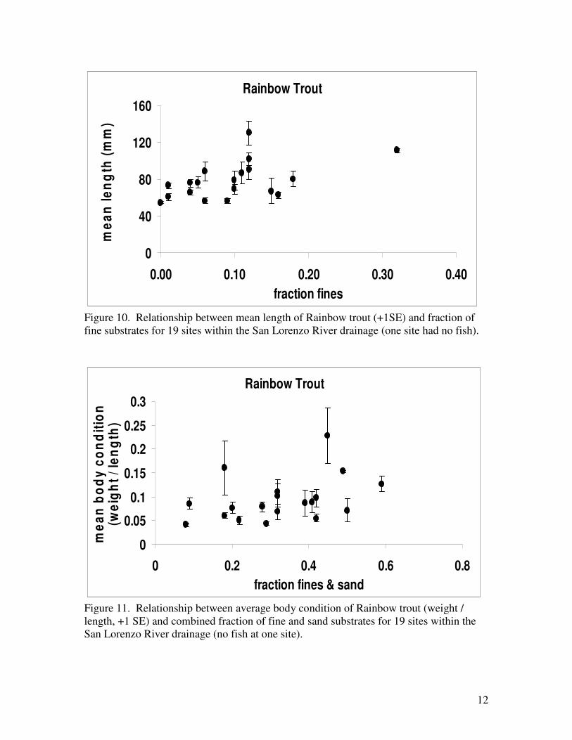
Rainbow trout (Oncorhynchus mykiss) steelhead density decreased as fine sediments increased (Figure 9). If less than 0.1 fish/m2 is taken as the lowest level of abundance for steelhead, this minimal density occurred in 9 of 11 cases above 6% fines, whereas sites having less fine sediment showed fish numbers exceeded this level in 6 of 8 cases. No relationship was exhibited between substrate quality and average length or body condition of rainbow trout (Figures 10, and 11).

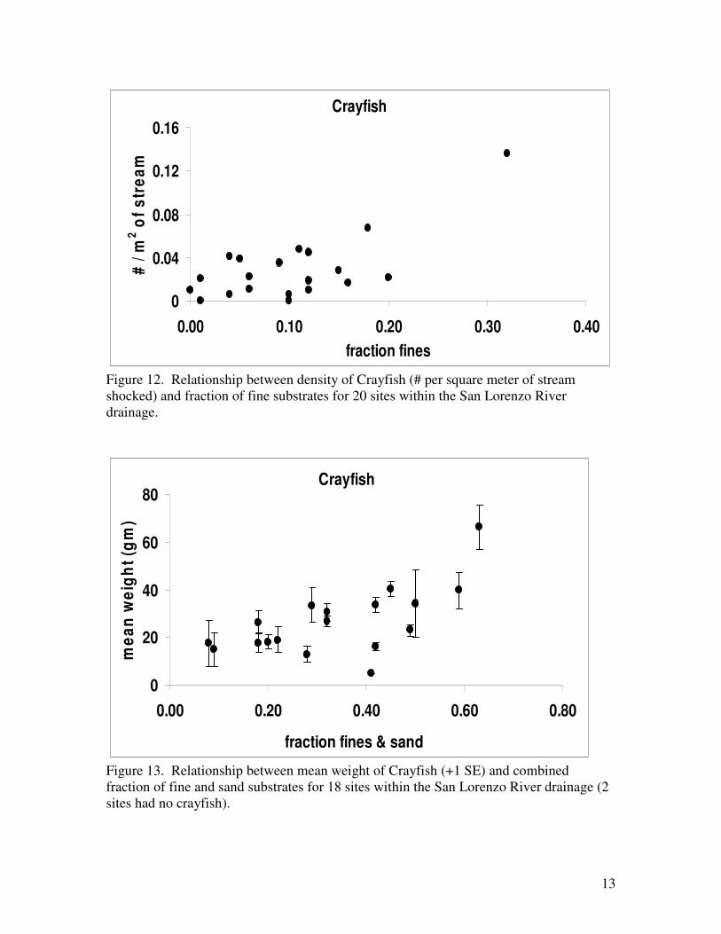
Crayfish (Pacifastacus leniusculus) density increased with fine sediment (Figure 12) and average weight of crayfish also increased with greater fine and sand sediment fraction cover (Figure 13). Conclusions

These results suggest that rainbow trout densities are limited by fine sediments above approximately 6% surface area cover, and that numbers and size of non-native crayfish are favored by increased levels of fine and sand sediment deposition. These crayfish are also known to have an important influence in consumption and processing of organic matter (leaf litter, detritus), and may limit the local abundance of native macroinvertebrates.

Rainbow trout

00.10.20.30.40.50.60.7

0.00 0.05 0.10 0.15 0.20 0.25 0.30 0.35fraction fines

# / m

2 of s

trea

m

Figure 9. Relationship between density of Rainbow trout (# per square meter of stream shocked) and fraction of fine substrates for 20 sites within the San Lorenzo River.

12

Rainbow Trout

0

40

80

120

160

0.00 0.10 0.20 0.30 0.40fraction fines

mea

n le

ngth

(mm

)

Figure 10. Relationship between mean length of Rainbow trout (+1SE) and fraction of fine substrates for 19 sites within the San Lorenzo River drainage (one site had no fish).

Rainbow Trout

0

0.05

0.1

0.15

0.2

0.25

0.3

0 0.2 0.4 0.6 0.8fraction fines & sand

mea

n bo

dy c

ondi

tion

(wei

ght /

leng

th)

Figure 11. Relationship between average body condition of Rainbow trout (weight / length, +1 SE) and combined fraction of fine and sand substrates for 19 sites within the San Lorenzo River drainage (no fish at one site).

13

Crayfish

0

0.04

0.08

0.12

0.16

0.00 0.10 0.20 0.30 0.40fraction fines

# / m

2 of s

trea

m

Figure 12. Relationship between density of Crayfish (# per square meter of stream shocked) and fraction of fine substrates for 20 sites within the San Lorenzo River drainage.

Crayfish

0

20

40

60

80

0.00 0.20 0.40 0.60 0.80

fraction fines & sand

mea

n w

eigh

t (g

m)

Figure 13. Relationship between mean weight of Crayfish (+1 SE) and combined fraction of fine and sand substrates for 18 sites within the San Lorenzo River drainage (2 sites had no crayfish).

14

4. Macroinvertebrate Community Metrics and Sediment Deposition

Using the reach-wide benthos (RWB) sampling methodology (SWAMP standard method), and the different methods for measuring sediment deposition at reach-scale and patch-scale, the responses of different community metrics to sediment were examined as simple univariate relationships of sediment cover to invertebrate diversity and tolerance. Based on the reference distribution alone, numeric guidance criteria for sediment deposition greater than the 75th and 90th percentiles of the reference distribution (Herbst et al. 2011) can be used to define impaired by bedded sediment as follows:

Sediment Indicator Moderately Disturbed [partially supporting]

(75/25)

Disturbed [not supporting]

(90/10) 1. Percent Fines (F) on transects >8.5% >15.2% 2. Percent Sand (S) on transects >27.5% >35.3% 3. Percent FS on transects >35.5% >42.0% 4. Percent FSG<8mm on transects >40.0% >50.2% 5. D50 median particles size <15 mm <7.7 mm 6. Percent patch-scale grid FS >28.8% >38.5% 7. Log RBS (relative bed stability) <−0.39 <−0.90

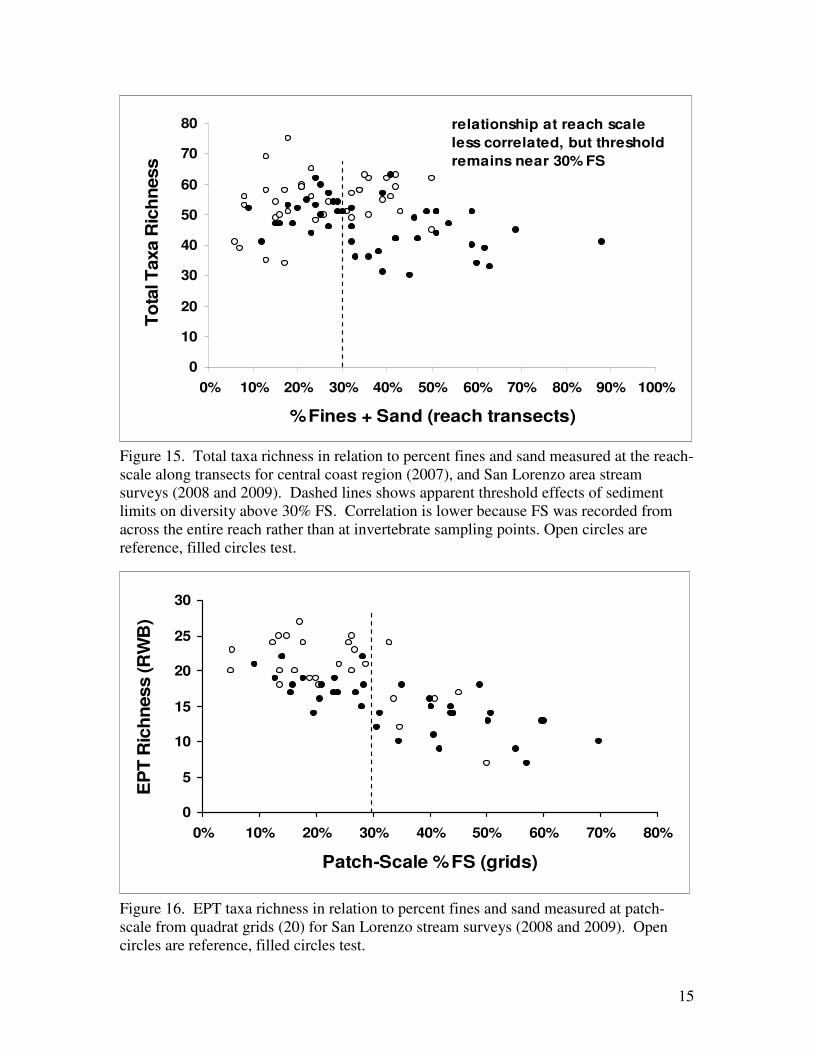
There is a clear loss of diversity with increased sediment deposition. This relationship is most pronounced when related to the patch-scale fines and sand measured at the locations of invertebrate sampling (Figure 14) than when measured at the reach scale (Figure 15).

0

10

20

30

40

50

60

70

80

0% 10% 20% 30% 40% 50% 60% 70% 80% 90% 100%

Patch-Scale %FS (grids)

Tota

l Tax

a R

ichn

ess

FS-grid measureswithin patchesof RWB samples

Figure 14. Total taxa richness in relation to percent fines and sand measured at the patch-scale using a 20x20 cm grid quadrat frame for all San Lorenzo area stream surveys (2008 and 2009). Dashed lines show apparent threshold effects of sediment limits on diversity above 30% FS. Open circles are reference, filled circles test.

15

0

10

20

30

40

50

60

70

80

0% 10% 20% 30% 40% 50% 60% 70% 80% 90% 100%

%Fines + Sand (reach transects)

To

tal T

axa

Ric

hne

ss

relationship at reach scaleless correlated, but thresholdremains near 30% FS

Figure 15. Total taxa richness in relation to percent fines and sand measured at the reach-scale along transects for central coast region (2007), and San Lorenzo area stream surveys (2008 and 2009). Dashed lines shows apparent threshold effects of sediment limits on diversity above 30% FS. Correlation is lower because FS was recorded from across the entire reach rather than at invertebrate sampling points. Open circles are reference, filled circles test.

0

5

10

15

20

25

30

0% 10% 20% 30% 40% 50% 60% 70% 80%

Patch-Scale %FS (grids)

EP

T R

ichn

ess

(RW

B)

Figure 16. EPT taxa richness in relation to percent fines and sand measured at patch-scale from quadrat grids (20) for San Lorenzo stream surveys (2008 and 2009). Open circles are reference, filled circles test.

16

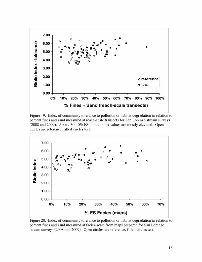
These changes in diversity at threshold levels provides evidence for the limiting effect of sediment deposition on biological integrity. In particular the influence of percent fines and sand (%FS) measured at different spatial scales (reach, patch, facies) was apparent above a range of 30-40% (Figures 14-22). Thresholds for impairment are shown at breaks in data distribution above 30% for patch-scale %FS (Figure 14) and reach-scale %FS (Figure 15) for total richness falling below 50 taxa, which also corresponds to the 25th percentile of the reference distribution (see Appendix). This 25th percentile of measures of biological integrity is the level that was used in EPA’s Western Stream Assessment (Stoddard et al. 2005) to define an impaired state of moderate disturbance to separate from streams above this level that support the reference least-disturbed condition. The taxa belonging to the mayfly, stonefly, and caddisfly groups (EPT) are often regarded as the most sensitive stream invertebrates, requiring clean, flowing, cold, stable stream bed conditions to thrive. Above 30% patch FS and 40% reach FS, much of the EPT richness falls below 15 taxa (Figure 16, 25th percentile reference =16.5 EPT). Increasing the small particle measure of deposition to include gravel 2-8 mm (%FSG<8mm), the level increases to 50% where most sites fall below 15 taxa. The percent of individuals in the community comprised by EPT taxa also responds above 30% patch-scale (Figure 17) and reach-scale FS (Figure 18), but at the reach-scale there also appears to be an optimum between 20-30% FS, with the fraction EPT declining both above and below this range. The biotic index measure of composite community pollution tolerance increases (more pollution-tolerant individuals present) as both reach- and facies-scale measures of %FS increase (Figures 19 and 20), and again change most above 30%. The percent of individuals defined as tolerant (tolerance values 7 to 10) increase markedly above 30% patch-scale FS (Figure 21), with only 15% of sites exceeding 25% tolerant below this sediment level, but above this 44% of sites have more than 25% tolerant individuals present (75th percentile of reference at 26.3% tolerant). The number of sensitive taxa (tolerance values 0-2) also shifts most at 30% patch-scale FS, with 94% of sites having 10 or more sensitive taxa below this FS level (25th reference percentile 9.5 sensitive taxa), and just 40% of sites above this level (Figure 22).

As with the sediment deposition indicators of impairment, the poorest quartile of the reference distribution can be used as a criterion for biological indicators of impaired condition. Using the lowest quartile (25%) of biological performance of the reference stream range to indicate impairment is supported by correspondence with the observed threshold levels of most biotic responses to sediment deposition (see Appendix for criterion levels of selected indicators). Combining sediment indicators with biological indicators provides a system for prioritizing sites for sediment control and restoration where more than half of indicators of both types are exceeded (red-flags in Appendix). Where sediment but not biological indicators are exceeded suggests that biological communities have either adapted to potential sediment limitations or are in transition and should be re-evaluated periodically. Where biological but not sediment indicators are exceeded suggests that limitations may be produced by stressors other than sediments or only partly by sediments. Stressor identification procedures may be useful in such cases (USEPA 2000; CADDIS: http://www.epa.gov/caddis/). It is also important to recognize where natural sources of sedimentation cause red-flag warnings, such as at Scott Creek (Swanton) where tidal conditions may alter both the physical and biological conditions, and the Big Sur River where wildfire and dredging may have altered sediment flux.

17

0%

10%

20%

30%

40%

50%

60%

70%

80%

90%

0% 10% 20% 30% 40% 50% 60% 70% 80%

Patch-Scale %FS (grids)

%E

PT

of to

tal

Figure 17. Percent EPT of total invertebrate counts in relation to percent fines and sand measured at patch-scale from quadrat grids (20) for San Lorenzo stream surveys (2008 and 2009). Above 30%FS all samples fall below 40% EPT. Open circles are reference, filled circles test.

0%

10%

20%

30%

40%

50%

60%

70%

80%

90%

0% 10% 20% 30% 40% 50% 60% 70% 80%

Reach-Scale %FS (transects)

%E

PT

of to

tal

Figure 18. Percent EPT of total invertebrate counts in relation to percent fines and sand measured at rech-scale transects for San Lorenzo stream surveys (2008 and 2009). Optimum at 20-30% FS, with limits on EPT apparent as %FS increases above 30% or decreases below 20%. Open circles are reference, filled circles test.

18

0.00

1.00

2.00

3.00

4.00

5.00

6.00

7.00

0% 10% 20% 30% 40% 50% 60% 70% 80% 90% 100%

% Fines + Sand (reach-scale transects)

Bio

tic In

dex

- tol

eran

ce

reference

test

Figure 19. Index of community tolerance to pollution or habitat degradation in relation to percent fines and sand measured at reach-scale transects for San Lorenzo stream surveys (2008 and 2009). Above 30-40% FS, biotic index values are mostly elevated. Open circles are reference, filled circles test.

0.00

1.00

2.00

3.00

4.00

5.00

6.00

7.00

0% 10% 20% 30% 40% 50% 60% 70%

% FS Facies (maps)

Bio

tic In

dex

Figure 20. Index of community tolerance to pollution or habitat degradation in relation to percent fines and sand measured at facies-scale from maps prepared for San Lorenzo stream surveys (2008 and 2009). Open circles are reference, filled circles test.

19

0%

10%

20%

30%

40%

50%

60%

70%

80%

0% 10% 20% 30% 40% 50% 60% 70% 80%

Patch-Scale %FS (grids)

%To

lera

nt 7

-8-9

-10

(RW

B)

Figure 21. Percent of individuals in community that are considered tolerant of environmental pollution (tolerance values of 7-10) increases with the facies areas that are covered by fines and sand. Open circles are reference, filled circles test.

0

2

4

6

8

10

12

14

16

18

20

0% 10% 20% 30% 40% 50% 60% 70% 80%

Patch-Scale %FS (grids)

No.

of S

ensi

tive

(0-1

-2) T

axa

(RW

B)

Figure 22. Number of sensitive taxa (having tolerance values of 0 to 2) declines with increased level of patch-scale cover of fines and sand. Open circles are reference, filled circles test.

20

Statistical methods for NMDS ordinations NMDS provide a tool for visualizing the similarity between biological communities by how close they plot in ordination space. Taxa present at fewer than 20% of sites (15 of 84, or 12 of 60 for San Lorenzo sites only) were removed from analysis, and invertebrate densities were relativized in PC ORD using the general relativization procedure. An NMDS ordination was run in autopilot mode at medium resolution.

Figure 23. Community ordination showing geographic differences for 84 surveys from 2007 (solid circles) over the central coast region, 2008 (open squares) San Lorenzo and adjacent watersheds, and 2009 (grey squares) from the San Lorenzo only.

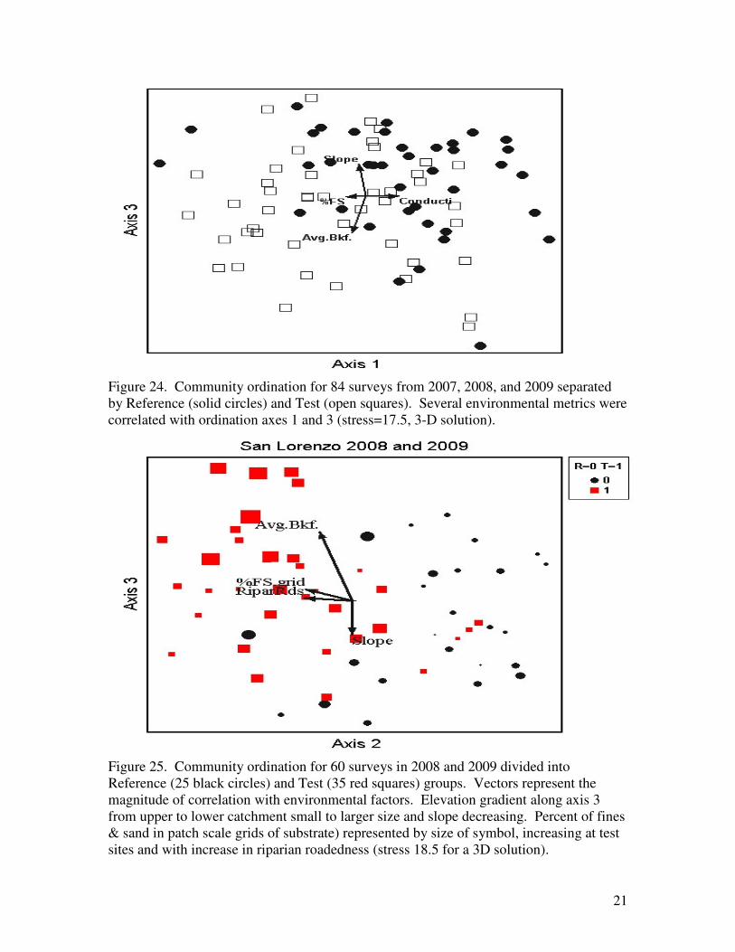
Community ordination similarity measures shows the geographic distinctions in taxonomic composition between the local San Lorenzo area and the larger central coast region (Figure 23). In addition to these biogeographic sources of variation in community structure, an examination of the contrasts between the combined central coast streams (Figure 24) and the San Lorenzo region streams (Figure 25) shows that reference and test sites are separated by environmental correlations with sediment fines and sand deposition (%FS), and with elevation from upper to lower watershed (from higher gradient or slope to greater average bankfull area, Avg.Bkf.). The streams with the most extensive cover of fines and sand (shown by symbol size in Figure 25) were also those that showed the most dissimilar community composition by separation in ordination space.

Sediment Tolerance In addition to ordinations showing community dissimilarities over environmental

gradients of sediment, individual taxa can be ranked according to their tolerance to sediment according to the abundance of each at different sediment levels. A listing of taxa by relative sediment tolerance is given at the end of this report.

21

Figure 24. Community ordination for 84 surveys from 2007, 2008, and 2009 separated by Reference (solid circles) and Test (open squares). Several environmental metrics were correlated with ordination axes 1 and 3 (stress=17.5, 3-D solution).

Figure 25. Community ordination for 60 surveys in 2008 and 2009 divided into Reference (25 black circles) and Test (35 red squares) groups. Vectors represent the magnitude of correlation with environmental factors. Elevation gradient along axis 3 from upper to lower catchment small to larger size and slope decreasing. Percent of fines & sand in patch scale grids of substrate) represented by size of symbol, increasing at test sites and with increase in riparian roadedness (stress 18.5 for a 3D solution).

22

Summary and Conclusions:

� Using data from the central coast ranges streams sampled in 2007, and the San Lorenzo area streams sampled in 2008 and 2009, the coverage of fines and sand measured at reach-, patch-, or facies-spatial scales of resolution (refer to Figure 1, showing these reflect increased spatial coverages of fines/sand deposits) all show limiting biological effects in terms of:

1. A progressive loss of total taxa diversity with increased sedimentation, where above about 30-40% FS, most sites fall below 50 taxa, while most streams are above this level of richness at less than 30% FS (Figures 14, 15).

2. Similarly, there is a loss of sensitive EPT taxa with increased %FS measured at grid frame patches in samples taken in San Lorenzo area streams in 2008 and 2009, showing a threshold above 30% FS results in the greatest collective loss of these insect groups from streams (Figure 16).

3. The fraction of individuals belonging to EPT taxa (%EPT) also declines markedly above 30% patch-scale FS (Figure 17) but there is some indication that an optimum level of reach-scale sediment may exist at 20-30% FS (Figure 18).

4. There is an increase in the community tolerance for pollution or degradation (Biotic Index) as the cover of fines and sand at the reach-scale or facies deposits increases (San Lorenzo area streams in 2008 and 2009; Figures 19, 20).

5. The shift to increased percent of tolerant organisms found in streams, or loss of sensitive taxa, occurs at a threshold level of 30% patch-scale FS (Figures 21, 22).

6. Community ordinations (NMDS plots) show that there were differences between years, primarily because of geographic differences in communities sampled in each year. Although each year shared sites within the San Lorenzo, sites sampled in 2007 came from as far south as the Sespe River and from both west and east sides of the coast range, and many sites in 2008 came from watersheds adjacent to the San Lorenzo – only in 2009 did all sites come from within the San Lorenzo (Figure 23)

7. Community ordinations also showed that for all years combined, there were separations between reference and test (Figure 24), but these were more pronounced when just the 2008-09 data of the San Lorenzo and adjacent watersheds are considered (Figure 25).

8. Surveys of native salmonids (rainbow trout or steelhead) conducted in 2009 showed that percent cover of fines above 6% appeared to limit the density of fish in the San Lorenzo River system (Figure 9). Non-native crayfish number and size increase with cover of fines and fines and sand (Figures 12, 13).

Using both sediment and biological exceedance criteria based on the reference range, and corresponding to thresholds of response of biological indicators to sediment, we conclude that these data provide a system for prioritizing streams for TMDL listing or de-listing, and for monitoring control of sediment sources. Streams that are on the 303(d) list for sediment could be removed if these numeric criteria are not exceeded, or a TMDL could be prepared if criteria are exceeded. Streams not on the 303(d) list might become listed if they exceed the numeric critera. Greater certainty in any judgments is incorporated when multiple biological and physical indicators are used.

23

References: Herbst, D.B., S.W. Roberts, R.B. Medhurst, and N.G. Hayden. 2011. Sediment

Deposition Relations to Watershed Land Use and Sediment Load Models Using a Reference Stream Approach to Develop Sediment TMDL Numeric Targets for the San Lorenzo River and Central Coast California Streams. Revised report to the Central Coast Regional Water Quality Control Board, January 2011.

Kaufmann, P.R, P. Levine, E.G. Robison, C. Seeliger, and D.V. Peck. 1999. Quantifying

Physical Habitat in Wadeable Streams. EPA/620/R-99/003. U.S. Environmental Protection Agency, Washington, D.C.

Stoddard, J.L., D.V. Peck, S.G. Paulsen, J. Van Sickle, C.P. Hawkins, A.T. Herlihy,

R.M. Hughes, P.R. Kaufmann, D.P. Larsen, G. Lomnicky, A.R. Olsen, S.A. Peterson, P.L. Ringold, and T.R. Whittier. 2005. An Ecological Assessment of Western Streams and Rivers. EPA 620/R-05/005, U.S. Environmental Protection Agency, Washington, DC.

US Environmental Protection Agency. 2000. Stressor Identification Guidance Document. Office of Water, EPA-822-B-00-025. Washington, D.C.

24

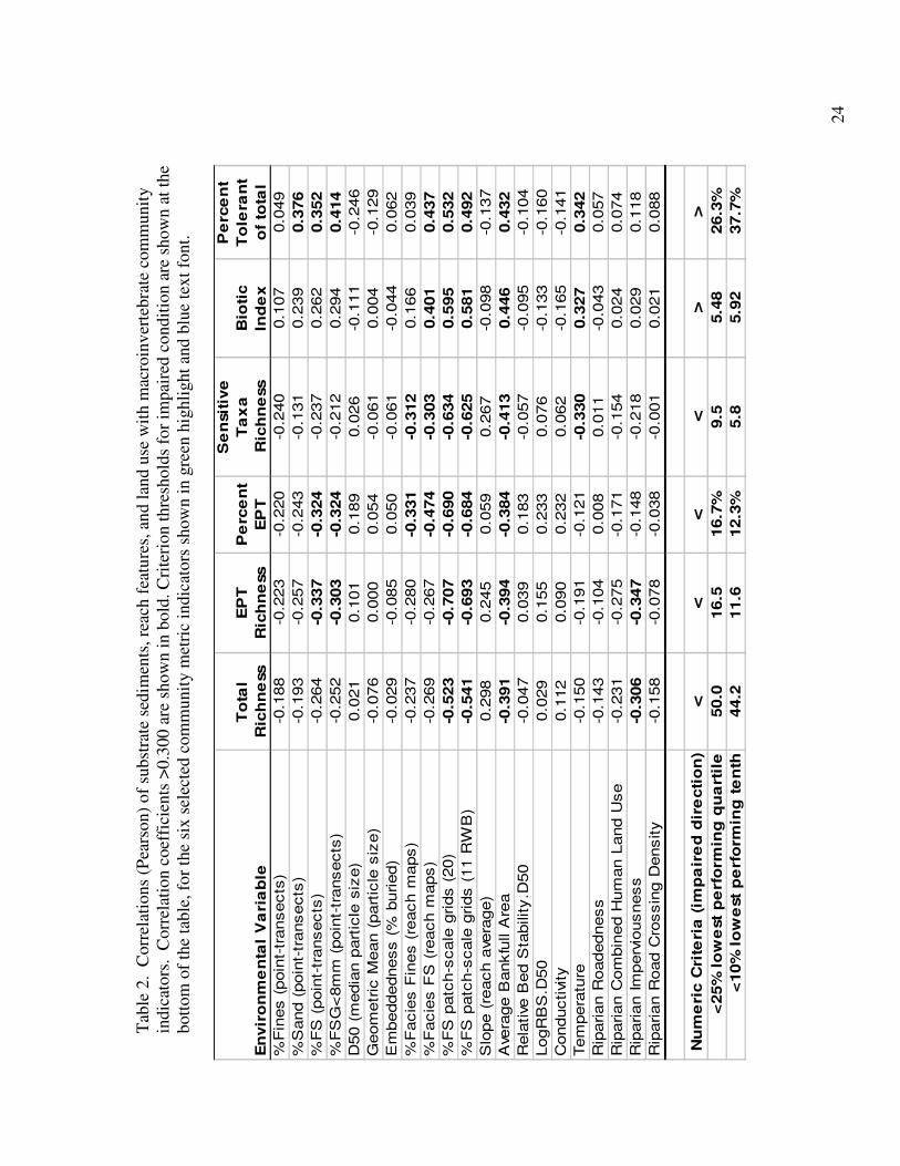
Tab

le 2

. C

orre

latio

ns (P

ears

on) o

f sub

stra

te s

edim

ents

, rea

ch fe

atur

es, a

nd la

nd u

se w

ith m

acro

inve

rteb

rate

com

mun

ity

indi

cato

rs.

Cor

rela

tion

coef

fici

ents

>0.

300

are

show

n in

bol

d. C

rite

rion

thre

shol

ds fo

r im

pair

ed c

ondi

tion

are

show

n at

the

botto

m o

f the

tabl

e, fo

r the

six

sel

ecte

d co

mm

unity

met

ric

indi

cato

rs s

how

n in

gre

en h

ighl

ight

and

blu

e te

xt fo

nt.

En

viro

nm

en

tal

Va

ria

ble

To

tal

Ric

hn

ess

EP

T

Ric

hn

ess

Pe

rce

nt

EP

T

Se

nsi

tive

T

ax

a

Ric

hn

ess

Bio

tic

Ind

ex

Pe

rce

nt

To

lera

nt

of

tota

l%

Fin

es (

poi

nt-

transe

cts

)-0

.188

-0.2

23

-0.2

20-0

.240

0.107

0.049

%S

and (

poin

t-tr

ans

ect

s)

-0.1

93

-0.2

57

-0.2

43-0

.131

0.239

0.37

6%

FS

(poin

t-tr

ans

ects

)-0

.264

-0.3

37-0

.324

-0.2

370.

262

0.35

2%

FS

G<

8mm

(po

int-

trans

ect

s)

-0.2

52

-0.3

03-0

.324

-0.2

120.

294

0.41

4D

50 (

med

ian p

articl

e s

ize)

0.0

210.

101

0.1

89

0.026

-0.1

11-0

.246

Geom

etr

ic M

ean

(part

icle

siz

e)

-0.0

76

0.000

0.0

54

-0.0

610.

004

-0.1

29

Em

bedd

edn

ess

(%

buried

)-0

.029

-0.0

85

0.0

50

-0.0

61-0

.044

0.062

%F

acie

s F

ines

(reac

h m

aps

)-0

.237

-0.2

80

-0.3

31-0

.312

0.166

0.039

%F

acie

s F

S (

reach

map

s)

-0.2

69

-0.2

67

-0.4

74-0

.303

0.40

10.

437

%F

S p

atc

h-s

cale

grids

(20

)-0

.523

-0.7

07-0

.690

-0.6

340.

595

0.53

2%

FS

patc

h-s

cale

grids

(11

RW

B)

-0.5

41-0

.693

-0.6

84-0

.625

0.58

10.

492

Slo

pe

(reach

ave

rage)

0.2

980.

245

0.0

59

0.267

-0.0

98-0

.137

Ave

rage B

ankfu

ll A

rea

-0.3

91-0

.394

-0.3

84-0

.413

0.44

60.

432

Rel

ativ

e B

ed S

tabili

ty.D

50-0

.047

0.039

0.1

83

-0.0

57-0

.095

-0.1

04

LogR

BS

.D50

0.0

290.

155

0.2

33

0.076

-0.1

33-0

.160

Con

duc

tivi

ty0.1

120.

090

0.2

32

0.062

-0.1

65-0

.141

Tem

pera

ture

-0.1

50

-0.1

91

-0.1

21-0

.330

0.32

70.

342

Rip

aria

n R

oad

ednes

s

-0.1

43

-0.1

04

0.0

08

0.011

-0.0

430.

057

Rip

aria

n C

om

bin

ed

Hum

an L

and U

se-0

.231

-0.2

75

-0.1

71-0

.154

0.024

0.074

Rip

aria

n Im

per

vious

nes

s-0

.306

-0.3

47-0

.148

-0.2

180.

029

0.118

Rip

aria

n R

oad

Cro

ssin

g D

ensity

-0.1

58

-0.0

78

-0.0

38-0

.001

0.021

0.088

Nu

me

ric

Cri

teri

a (

imp

air

ed

dir

ect

ion

)<

<<

<>

><

25%

lo

we

st p

erf

orm

ing

qu

art

ile

50.0

16.5

16.7

%9.

55.

4826

.3%

<10

% l

ow

est

pe

rfo

rmin

g t

en

th44

.211

.612

.3%

5.8

5.92

37.7

%

25

Map 1. Sites surveyed within the San Lorenzo River watershed in May-June of 2008 and 2009. Site numbers correspond to the code listings in Appendix..

8

7

20 19

17

15

21

22

23

18 6

5 11

27

24

0

1

2 3

16 4 9

10

12

13

14

25

26

26

Map 2. Sites surveyed outside of the San Lorenzo watershed in May-June of 2008 and 2009. Includes Aptos (inset), Scott, Waddell, and Pescadero Creeks (gray area is the boundary of the San Lorenzo). Site numbers correspond to the code listings in Appendix.

28

36 38

37 39

29

31

32

30

33 35

34

27

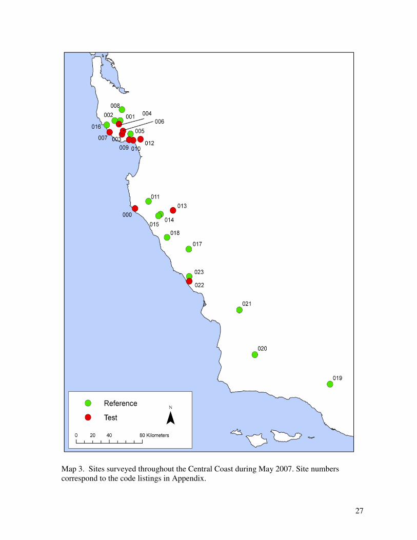
Map 3. Sites surveyed throughout the Central Coast during May 2007. Site numbers correspond to the code listings in Appendix.

28

Appendix. Biological metric and sediment exceedances (if > half of indicators exceeded, then red if both biological and physical, yellow if one or the other) – Reference sites.

Year R or T Stream Name Site Name Tota

l ric

hnes

s

EP

T ric

hnes

s

%E

PT

Bio

tic In

dex

Per

cent

Tol

eran

t

Sen

sitiv

e N

umbe

r

Bio

Indi

cato

rs E

xcee

ded

Dep

ositi

on E

xcee

danc

es

<25t

h %

bio

indi

cato

rs >

3

>75t

h %

Sed

imen

t if >

half

2008 R San Lorenzo River Brimblecom 58 24 51.2% 4.03 5.9% 19 0 02008 R San Lorenzo River Castle Rock 62 24 36.2% 4.70 31.3% 16 1 5 x2008 R Fall Creek Cowell SP 51 18 16.3% 5.78 47.1% 12 3 5 x2008 R Jamison Creek fire station 54 16 11.5% 5.64 28.0% 11 4 1 x2008 R Boulder Creek Hwy 236.4 58 20 61.0% 3.83 11.2% 16 0 02008 R Kings Creek County Land 48 20 77.4% 3.50 9.1% 12 1 22008 R Bear Creek treatment plant 57 24 48.9% 4.37 9.2% 18 0 22008 R Aptos Creek Rancho trail 50 12 16.2% 5.43 18.7% 7 3 5 x2008 R Waddell Creek Alder Camp 58 18 43.9% 4.79 16.6% 11 0 02008 R W. Waddell Creek confluence 56 25 72.8% 3.55 10.9% 19 0 12008 R E. Waddell Creek confluence 54 19 57.5% 3.74 11.9% 10 0 02008 R E. Waddell Creek treatment plant 58 23 35.9% 4.22 17.6% 16 0 32008 R Little Creek Swanton bridge 62 21 17.3% 5.29 41.3% 16 1 5 x2008 R Scott Creek Upper trib 51 16 16.5% 5.24 22.2% 12 2 32008 R Scott Creek Below Little 65 27 46.7% 3.89 10.2% 17 0 12008 R Pescadero Creek Cloverdale bdg 62 17 25.8% 5.20 22.1% 13 0 5 x2008 R Pescadero Creek Oakland YMCA 49 20 58.3% 3.60 8.9% 13 1 02008 R Pescadero Creek Sequoia trail 50 20 25.0% 5.11 19.3% 17 0 02008 R Peters Creek campground 59 25 64.7% 3.93 12.2% 19 0 02009 R Aptos Creek Rancho trail 45 7 6.5% 5.84 24.1% 6 5 7 x x2009 R Fall Creek Cowell SP 56 21 24.9% 4.31 10.9% 15 0 6 x2009 R Bear Creek treatment plant 51 19 59.2% 4.27 19.4% 15 0 12009 R San Lorenzo River Brimblecom 53 23 40.4% 4.33 9.2% 16 0 02009 R San Lorenzo River Castle Rock 59 24 33.6% 4.77 8.7% 16 0 6 x2009 R Kings Creek County Land 55 25 55.0% 4.49 18.6% 17 0 22007 R Kings Creek County Land 57 20 31.6% 4.96 21.6% 13 0 12007 R San Lorenzo R Campbell 63 23 38.0% 4.65 26.1% 15 0 4 x2007 R Soquel Cr Upper 63 19 37.5% 4.57 21.1% 12 0 02007 R Stevens Cr Reservoir 60 17 27.5% 5.05 11.1% 12 0 12007 R Carmel R Bluff Camp 41 13 13.5% 5.52 24.2% 7 5 0 x2007 R Arroyo Seco day use area 39 10 5.9% 6.25 36.8% 5 6 0 x2007 R Tassajara Cr Horse trail 35 12 18.4% 5.58 12.4% 8 4 0 x2007 R Waddell Cr Alder Camp 49 15 12.5% 5.13 12.7% 9 4 0 x2007 R San Antonio R Interlake Bridge 69 17 13.0% 6.34 51.2% 7 4 0 x2007 R Nacimiento Cr Campground 56 19 26.5% 4.98 20.8% 17 0 12007 R Sespe Cr Lion 59 17 31.7% 5.81 28.2% 5 3 12007 R Sisquoc R Above Dam 34 10 16.9% 6.52 59.7% 2 5 1 x2007 R Salinas R CDF Station 50 10 10.0% 6.32 36.8% 2 5 0 x2007 R San Simeon Cr Above Fence 75 24 60.7% 4.63 26.6% 19 1 1

bioindicator criteria <25th percentile 50.0 16.5 16.7% 5.48 26.3% 9.5<10th percentile 44.2 11.6 12.3% 5.92 37.7% 5.8

direction of impairment < < < > > <

29

Appendix (continued). Biological metric and sediment exceedances (if > half of indicators exceeded, then red if both biological and physical, yellow if one or the other) – Test sites.

Year R or T Stream Name Site Name Tota

l ric

hnes

s

EP

T ric

hnes

s

%E

PT

Bio

tic In

dex

Per

cent

Tol

eran

t

Sen

sitiv

e N

umbe

r

Bio

Indi

cato

rs E

xcee

ded

Dep

ositi

on E

xcee

danc

es

<25t

h %

bio

indi

cato

rs >

3

>75t

h %

Sed

imen

t if >

half

2008 T San Lorenzo River city intake 40 13 20.9% 6.46 64.4% 7 5 7 x x2008 T San Lorenzo River Paradise 42 12 26.0% 5.74 48.3% 8 5 5 x x2008 T San Lorenzo River RR bridge 42 15 12.3% 6.26 58.8% 11 5 5 x x2008 T San Lorenzo River entrance bdg 45 10 4.6% 6.02 49.0% 8 6 7 x x2008 T San Lorenzo River San Lo Way 63 22 38.9% 4.96 24.4% 15 0 32008 T San Lorenzo River Hwy 9 X 57 18 39.2% 5.39 19.2% 13 0 5 x2008 T San Lorenzo River E Lomond bdg 54 22 31.0% 5.18 9.0% 15 0 12008 T Zayante Creek RR bridge 46 17 20.4% 5.33 27.1% 13 2 02008 T Zayante Creek Quail Hollow 38 18 7.3% 5.77 12.4% 11 3 7 x2008 T Lompico Creek Lompico bdg 57 14 31.8% 4.51 19.6% 12 1 02008 T Zayante Creek Market bdg 47 18 23.8% 4.86 8.3% 15 1 22008 T Bean Creek Locateli Rd. 34 13 16.3% 5.35 40.8% 7 5 6 x x2008 T Bean Creek Morgan Runs 51 19 61.5% 4.29 16.8% 14 0 32008 T Love Creek Glen Arbor bdg 53 17 21.0% 5.03 7.0% 12 0 12008 T Boulder Creek Hwy 9 47 14 60.4% 5.39 19.4% 7 3 22008 T Bear Creek Eurella 50 18 49.8% 4.28 11.2% 14 0 02008 T Newell Creek Rancho Rio Rd. 51 15 26.0% 4.68 9.1% 8 2 8 x2008 T Carbonera Creek Carbonera Rd 36 9 26.4% 4.77 39.3% 9 4 4 x2008 T Branciforte Creek DeLaveaga 51 14 21.5% 4.99 21.2% 11 1 8 x2008 T Branciforte Creek Shady Brook bdg 49 16 29.4% 5.21 15.1% 12 2 6 x2008 T Shingle Mill Creek Above Hwy 9 47 14 15.0% 5.49 36.6% 9 6 6 x x2009 T San Lorenzo River Paradise 46 10 33.1% 5.50 35.5% 8 5 3 x2009 T San Lorenzo River city intake 33 7 11.4% 6.63 71.1% 4 6 6 x x2009 T San Lorenzo River RR bridge 30 11 11.4% 6.04 53.0% 5 6 5 x x2009 T Bean Creek Locateli Rd. 51 14 17.6% 4.57 17.3% 10 1 7 x2009 T Bean Creek Morgan Runs 52 18 45.5% 4.59 17.5% 13 0 02009 T Carbonera Creek Carbonera Rd. 41 9 25.7% 4.90 23.8% 7 3 32009 T Branciforte Creek DeLaveaga 51 15 32.2% 4.44 11.2% 8 2 8 x2009 T San Lorenzo River entrance bdg 42 13 5.3% 5.77 41.3% 7 6 4 x2009 T San Lorenzo River San Lo Way 51 19 38.5% 4.84 16.4% 12 0 22009 T Boulder Creek Hwy 9 52 16 22.9% 5.25 20.6% 10 1 02009 T Bear Creek Eurella 55 19 53.6% 3.64 13.4% 12 0 12009 T Zayante Creek RR bridge 54 17 28.9% 4.92 14.5% 13 0 02009 T San Lorenzo River Hwy 9 X 52 17 27.3% 5.48 23.5% 9 1 02009 T San Lorenzo River E Lomond bdg 53 21 34.8% 4.79 14.1% 12 0 02007 T Big Sur River Coyote Flat 39 8 9.5% 5.78 23.5% 5 5 6 x x2007 T San Lorenzo R RR bridge 44 11 10.0% 5.06 25.5% 8 4 5 x x2007 T Bear Cr Scout Camp 60 21 58.8% 3.76 13.1% 14 0 02007 T Zayante Creek RR bridge 62 18 24.4% 4.86 20.4% 13 0 12007 T Scott Cr Swanton 31 9 1.5% 6.08 30.1% 6 6 4 x x2007 T Soquel Cr Lower 36 8 1.5% 5.45 24.0% 3 4 2 x2007 T Aptos Cr Valencia 41 6 23.5% 5.57 29.0% 4 5 5 x x2007 T Corralitos Cr Hames 47 12 6.7% 5.50 28.8% 8 6 0 x2007 T Arroyo Seco Green Bridge 41 11 25.7% 5.65 30.5% 4 5 1 x2007 T Santa Rosa Cr High School 44 10 21.0% 4.72 20.5% 4 3 2

30

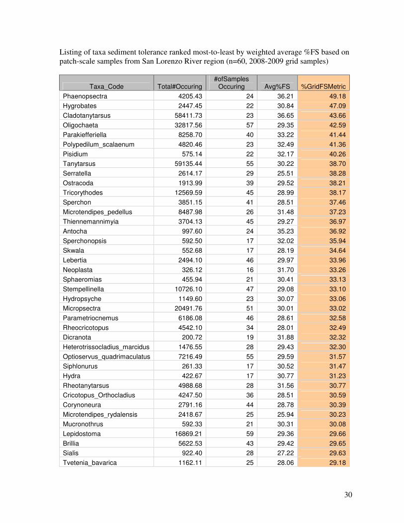
Listing of taxa sediment tolerance ranked most-to-least by weighted average %FS based on patch-scale samples from San Lorenzo River region (n=60, 2008-2009 grid samples)

Taxa_Code Total#Occuring #ofSamples

Occuring Avg%FS %GridFSMetric Phaenopsectra 4205.43 24 36.21 49.18 Hygrobates 2447.45 22 30.84 47.09 Cladotanytarsus 58411.73 23 36.65 43.66 Oligochaeta 32817.56 57 29.35 42.59 Parakiefferiella 8258.70 40 33.22 41.44 Polypedilum_scalaenum 4820.46 23 32.49 41.36 Pisidium 575.14 22 32.17 40.26 Tanytarsus 59135.44 55 30.22 38.70 Serratella 2614.17 29 25.51 38.28 Ostracoda 1913.99 39 29.52 38.21 Tricorythodes 12569.59 45 28.99 38.17 Sperchon 3851.15 41 28.51 37.46 Microtendipes_pedellus 8487.98 26 31.48 37.23 Thiennemannimyia 3704.13 45 29.27 36.97 Antocha 997.60 24 35.23 36.92 Sperchonopsis 592.50 17 32.02 35.94 Skwala 552.68 17 28.19 34.64 Lebertia 2494.10 46 29.97 33.96 Neoplasta 326.12 16 31.70 33.26 Sphaeromias 455.94 21 30.41 33.13 Stempellinella 10726.10 47 29.08 33.10 Hydropsyche 1149.60 23 30.07 33.06 Micropsectra 20491.76 51 30.01 33.02 Parametriocnemus 6186.08 46 28.61 32.58 Rheocricotopus 4542.10 34 28.01 32.49 Dicranota 200.72 19 31.88 32.32 Heterotrissocladius_marcidus 1476.55 28 29.43 32.30 Optioservus_quadrimaculatus 7216.49 55 29.59 31.57 Siphlonurus 261.33 17 30.52 31.47 Hydra 422.67 17 30.77 31.23 Rheotanytarsus 4988.68 28 31.56 30.77 Cricotopus_Orthocladius 4247.50 36 28.51 30.59 Corynoneura 2791.16 44 28.78 30.39 Microtendipes_rydalensis 2418.67 25 25.94 30.23 Mucronothrus 592.33 21 30.31 30.08 Lepidostoma 16869.21 59 29.36 29.66 Brillia 5622.53 43 29.42 29.65 Sialis 922.40 28 27.22 29.63 Tvetenia_bavarica 1162.11 25 28.06 29.18

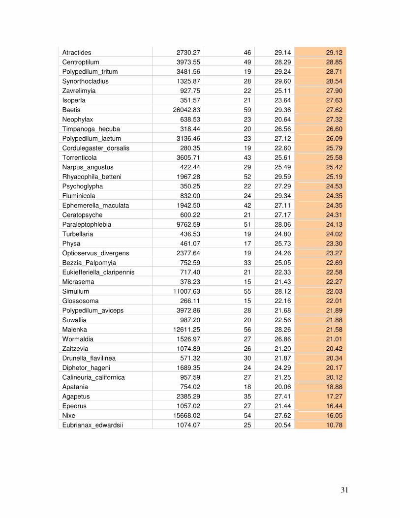
31

Atractides 2730.27 46 29.14 29.12 Centroptilum 3973.55 49 28.29 28.85 Polypedilum_tritum 3481.56 19 29.24 28.71 Synorthocladius 1325.87 28 29.60 28.54 Zavrelimyia 927.75 22 25.11 27.90 Isoperla 351.57 21 23.64 27.63 Baetis 26042.83 59 29.36 27.62 Neophylax 638.53 23 20.64 27.32 Timpanoga_hecuba 318.44 20 26.56 26.60 Polypedilum_laetum 3136.46 23 27.12 26.09 Cordulegaster_dorsalis 280.35 19 22.60 25.79 Torrenticola 3605.71 43 25.61 25.58 Narpus_angustus 422.44 29 25.49 25.42 Rhyacophila_betteni 1967.28 52 29.59 25.19 Psychoglypha 350.25 22 27.29 24.53 Fluminicola 832.00 24 29.34 24.35 Ephemerella_maculata 1942.50 42 27.11 24.35 Ceratopsyche 600.22 21 27.17 24.31 Paraleptophlebia 9762.59 51 28.06 24.13 Turbellaria 436.53 19 24.80 24.02 Physa 461.07 17 25.73 23.30 Optioservus_divergens 2377.64 19 24.26 23.27 Bezzia_Palpomyia 752.59 33 25.05 22.69 Eukiefferiella_claripennis 717.40 21 22.33 22.58 Micrasema 378.23 15 21.43 22.27 Simulium 11007.63 55 28.12 22.03 Glossosoma 266.11 15 22.16 22.01 Polypedilum_aviceps 3972.86 28 21.68 21.89 Suwallia 987.20 20 22.56 21.88 Malenka 12611.25 56 28.26 21.58 Wormaldia 1526.97 27 26.86 21.01 Zaitzevia 1074.89 26 21.20 20.42 Drunella_flavilinea 571.32 30 21.87 20.34 Diphetor_hageni 1689.35 24 24.29 20.17 Calineuria_californica 957.59 27 21.25 20.12 Apatania 754.02 18 20.06 18.88 Agapetus 2385.29 35 27.41 17.27 Epeorus 1057.02 27 21.44 16.44 Nixe 15668.02 54 27.62 16.05 Eubrianax_edwardsii 1074.07 25 20.54 10.78