“{ ‘TABLE OF CONTENTS

RN Page

Number 4 P

ACKNOWLEDGEMENTSA

ii N1

INTRODUCTION _ 1_

CHAPTER I THE MOTION OF A PARTICLE IN A 5POSITIONAL FIELD OF FORCE IN A

" EUCLIDEAN SPACE En OF DIMENSIONn Z 2 .

U6

1. Dynamical trajectories in a 5Euclidean space En of

i .dimension n Z 2 . ”

2. The system of explicit 9equations of dynamicaltrajectories.

3. Actual and virtual dynamical IOtrajectories.

CHAPTER II GEOMETRICAL PRELIMINARIES AND 12APPELL'S‘TRANSFORMATION.4. Hyperplanes in En . 12 {5. Collineations in a projective 14

space Su of dimension n Z 2 . {6. Appe1l's transformation. 16A

iii _

· PageNumber, 2

CHAPTER III SOME GEOMETRICAL RESULTS CONCERNING 25_

iDYNAMICAL TRAJECTORIES IN A EUCLIDEANSPACE E3 OF THREE DIMENSIONS. °

•7.The arc length derivatives of a 25

— positional field of force in E3 .8. The system SO of dynamical

T29

trajectories of a positionalfield of force. A l T

9. A study of the curvature and 33the torsion of a dynamical

trajectory .4 10. Rest trajectories. 35

CHAPTER IV HALPHEN'S THEOREM AND SOME RELATED 39RESULTS IN E3 . y 'll. The conditions for a planar 39

dynamical trajectory in E3 . f12. Halphen'$ Theorem . 4213. The notion of a flat point of _ 47 ·

·« a positional field of force in E3.

————"”———————r-———————r"———————————__"——”‘——___*———————————————————*————————*——

. - Y _ 1A

Page· ~ Number

y 14. The theory of a flat point of 51‘

a dynamical trajectory of a_ positional field of force in E3.

· 15. A study of the quadric coneQhof

S5Theorem 14.2 .

CHAPTER V SOME RESULTS CONCERNING HELICAL 59_ TRAJECTORIES IN E3 . 7

16. The theory of helices in a S9" Euclidean space E3 . _17. A study of the conditions for 63

a helical trajectory in a ·~ positional field of force in E3 .18. A study of the dynamical 67

4

trajectories in E3 that arelocally helical.

19. A further study of the 72 T

dynamical trajectories in E33

that satisfy equation(18.7)CHAPTER

VI HALPHEN'S THEOREM IN A EUCLIDEAN . 76

g _ SPACE E„ . . _4

.

‘ UPage O·”

_ NumberT A

20. Conditions for a curve in E„ 76‘to be contained in a k—flat,with

kl=2 or 3 . E

·Z1. ”Positiona1 fields of force in 81

E„ that generate planardynamical trajectories .

° 22. .Positional fields of force in 89E„ that generate 3-flat

g dynamical trajectories .lCHAPTER VII POSITIONAL FIELDS OF FORCE IN En 97

THAT RESTRICT PARTICLE MOTION TO9(k+l)—FLATS . ·23. Positional fields of force 97

that are k-dimensional parallel.24. An additional property of 100 ’·

7

motion in a k—dimensiona1—

parallel positional field offorce .-

g.

' ' 25. A characterization of 102·

hkadimensional parallel fields

* of force .

I so „ 1

PageNumber'

26. Positional fields of force 103that are (k-1)—dimensiona1

central ._27. An extension of Kep1er's 107

V second law of motion .28. A characterization of 110

(k-1)-central positional fieldsof force.

P29. An additional property of 112

—8

k-parallel and (k-l)·centra1fields of force in En .8

BIBLIOGRAPHYe 117

VITA 120

lV ‘I§TRDDUCTION

A1 This research effort Was initiated to ekplore the lpossibility of ektending a dynamical theorem due to_,G.

Halphen. Halphen's Theorem states that, "Every dynamical

trajectory in a positional field of force in E3 is planar,

if and only if the force field is either parallel or central".

Although Halphen's Theorem has been known for some time,

a search of the available literature did not reveal a complete

proof of the result. It is well known and well documented

that every dynamical trajectory in a parallel or central

field of force is planar; however, the same cannot be said

of the converse implication.

~ The published works of Dr. Edward Kasner and

Dr. John DeCicco served as the primary reference materialA

for this paper. Several of their classical results are

contained in Chapter I, which serves as an orientation

chapter.

p Chapters II and III were designed to support later

chapters. A transformation is developed in Chapter II thatIi

is used in Chapter VII to show the projective similarity

between k-parallel and (k—l)-central fields of force.

Chapter III contains several calculational formulas that

1 · r

2„”

Aare useful in Chapters IV and V.. j

A new analytic proof of the proposition that a field of

force in B, is either parallel or central if and only if the

dynamical trajectories are all plane curves, is presented in _Chapter IV. The details of this proof suggested the new

concepts of a flat point in a field of force and a flat

point on a dynamical trajectory in a field of force, and

these led to various new results related to Halphen's

Theorem. One of the more important new results in this

setting is a less restrictive version of Halphen's Theorem pwhich states that, "At every point P of a positional field

of force, in E3 there exists six distinct directions, not allof which are on a quadric cone with vertex at P, such that

[ each dynamical trajectory which passes through the pointP4

in one of these six directions is flat at the point P, if

and only if the field of force is either parallel or central".

It is trivially true that every plane curve is a helix.i

This suggested that additional results related to Halphen’s QTheorem could be obtained by considering those fields of

force in which every dynamical trajectory is a helix. The

results obtained under this condition are contained in

Chapter V.On the basis of these findings the new concept of a

Helical point of a positional field of force was defined.

‘ 3

· One of the more interesting new results obtained from thiseffort states that, "If the point P is not a helical point

_

of a positional field of force in E3 , then in each{

ldirection through P there passes at most two dynamical _

trajectories which have the point P as a helical point". _A close analysis of Halphen's Theorem revealed that the

key concepts which required redefinition in order to make a ‘ l

non trivial extension to higher dimensional space possible,.

were those of a parallel and central field of force. In this4 connection, definitions were structured for a k-dimensional

parallel field of force and a (k—l)—dimensiona1 central field

of force in a Euclidean space of n—dimensions with 1 i k < n.

These definitions were then used to obtain an extension of4

Halphen's Theorem to a Euclidean space of 4-dimensions which4

states that, "Every dynamical trajectory in a positional

field of force in E, is contained in some k—flat, withi

k = 2,3, if and only if the field of force is either

(k—l)-parallel or (k—2)—centra1". This new result

iscontainedin Chapter VI. C ‘

Although it is firmly believed that Halphen's Theorem

v is extendable to a Euclidean space of n—dimensions with sn > 4, no complete proof has as yet been developed. A

partial extension is presented in Chapter VII. This result

states that "Every dynamical trajectory in a k-dimensional

V 4. parallel or a (k-l)—dimensional central positional field of

force in En with k é n « 1, is contained in some' s(k+1)-dimensionalhyperplane".The

applicability of the new definitions of a k-parallel

‘and (k—l)—central fields of force was further established by

i extending other classical dynamical results in E3 to spaces

of higher dimension. The most noteworthy new result obtained ·

in this setting is an extension of Kepler's second law of Vmotion which states that, "In a (k-l)~dimensional central

field of force in En with k i n-l and a fixed(k-l)—dimensional hyperplane, L£_1 , as center, the time

required in going from point P to point Q along a fixed

dynamical trajectory is proportional to the vectorial area

OPOQO swept out by the radius vector of the orthogonal

projection of the dynamical trajectory on a plane orthogonal

to Lg_1 . The point 0 is the projection of the central flat

in the projection plane".The proof of Halphen's Theorem in both E3 and E„ led to ’

the consideration of quadrics. It is strongly anticipatedJ

_ that the generalization of En for n > 4, will also involve

quadrics in En . ‘ é

———————·——————**——————"—’————’“———’——’——“""”——————————’——————————"'——————————1‘ 11 EI 1

° 'CHAPTBR II°‘THE‘M0TIONTOF;A°RARTICLE'IN„A'PO§§TIONAL‘FIELD°OF‘FORCE

..IN A EUCLIDEAN SRÄCB ER OF DIMENSIONÄn“é;2. ‘

1...Dynamical.trajectories.in.a1Fuclidean.spaceÄBnÄofII2 . I I

This development begins with the presentation of basicintroductory material. This material, for the most part,was suggested by the works of Professors E. Kasner and

”

J. DeCicco.I

*Consider a particle of mass m moving in a Euclidean

space En of dimensieh n 3_2, such that the laws governingthis motion are Newtonian. That is, with the proper choiceof units of measurement, the mass of the particle

r multiplied by its acceleration, is equal to the force.In Eh , let x = (x1,x2,...,xn) denote cartesian

Icoordinates of a point, and let F = (F1,F2,...,Fn) be therectangular components of a force vector acting on theparticle situated at the position x.

Definition 1.1. If the force vector F is a single Tvalued and continuous vector function of x such that it Ipossesses continuous partial derivatives of at least the :

_ first order in a certain region of En and F is not II‘identically zero in this region, then this physical

:configuration is called a statignary or positiona1_fie1d 1

'°of°force. l Is Q

I

w . 6»

For a discussion of this and other fields of force inE, and E3 see Kasner [1], and Kasner and DeCicco°[2.7].e

The following definition can be found in [2].J

°°Hefinition’1.2. A Faraday'line°of°force in a givenN

positional field of force is•a curve C of the region that has· its tangent at each of its points parallel to the corresponding

force vector at that point.l-

° This concept of lines of force was first introduced by

Faraday, and is of fundamental importance in the mathematical

theory of electricity and magnetism.The lines of force are by definition the solutions to the ‘

following set of ordinary defferential equations of first

order:' . dx.‘ (1.1) . xi = —H%—= aFi ,

where 1 j_i i n, the dot represents the derivative withrespect to a continuously varying parameter other than time,

and a is a non-zero scalar.The solution of equation (1.1) gives rise to n constants ,

of integration. However, only (n—l) of these constants are[

·( essential.

An existence and uniqueness theorem [4,5] on systems of( differential equations states that the solution to (1.1) for

a given set of initial conditions is unique. In other words,

through any point x of th€_given„region,_there passes

oneandonly one line of force. ·

If C is the unique line of force which passes through

the point xo , then through any other point xl of C there

passes a unique line of force, namely C. Because of this

fact the number of essential constants is (n-1) and the set

of lines of force in En is (n—l)-fold infinite.Thus,accordingto the notation of Kasner [6] there are wn_l

Faraday lines of force in En. ° U

‘ [The following definition can be found in [8] and [9].‘ °°Definition 1.3. A dynamical trajectory is the path of

a freely moving particle in a positional field of force.

[Under the previously discussed conditions, the motion

of a freely moving particle of mass m is described by the

[ following system of n ä 2, differential equations

mxlmx,

mxn = Fn(xl,x2,...,xH), =where the dots represent derivatives with respect to a

continuously varying parameter such as time.

\|{

8[

°°Definition 1.4. The set of all solutions to the _

· system (1.2) is defined to be a dynamical system S0. .

A more detailed discussion of dynamical systems So can

be found in [14].I

I"Theorem‘1;l. Related to a given positional field of

..force.E.with.]F| > 0, of Euclidean space Eu of dimension

there is a dynamical system So of wZH—1dynamical°trajectories

C.‘

For, solving such a system of differential equations,

Zn constants are introduced. However, not all of these

(constants are essential. By appealing to an existence and

uniqueness theorem [4,5] on systems of ordinary differential

equations, it is found that the solution C, corresponding to

‘ a particular choice of the Zn constants (that is, the initial

position and the initial velocity) is unique. Thus a given

dynamical trajectory C may be generated hy selecting any of

its points as initial position and the proper initial

velocity at that point. The set of points that a given Tdynamical trajectory C passes through is one-fold infinite.

This would imply that for a given set of initial conditions

there are wl other initial conditions which will generateU

the game dynamical trajectory C. .

The preceding agrument implies that the number of

essential constants is (Zn — 1) and the set of all

'“dXnamical trajectories satisfying equation (1.2) is[

°‘(2n°¥“l)°fold infinite. ° ·

Consequently, the validity of Theorem 1.1,

isestablished.‘

'2 2. The system of explicity eguations of dynamicaltrajectories. The problem under consideration involves

the geometric properties of dynamical trajectories. In _

- order to study such properties, it is sometimes helpful toN

eliminate the parameter t, from equations(1.2).(

This can be done by first using the implicit function

theorem to find that the equations of the dynamical

trajectory can be expressed in terms of the independent

variable xi, for sime i. Suppose it is found that xl is

I such an independent variable. Then the chain rule can be T

- used to express the system (1.2) in terms of derivatives

‘with respect to xl which will be denoted by primes. This

process leads to[F2 - x2Fl] xx = [Fi - xlFl] xg,

for i = 3,4,..„n, where F2 - x2 Fl is assumed to be not zero. T

By differentiating equations (2.1) with respect to xl,

the following equations free from the parameter t, are

obtained: Ix BF n BF

(L2) (Fl - xl

xlfori = 2,3,...,n.

‘ In describing the dynamical trajectories the equations

(2.2) for i= 3,4,...,n are unnecessary as they are —_

dependent on equations (2.1) and (2.2) for i = 2. These Zresults are summarized in the following theorem.

. ° Theorem 2.1. The system S0 of w2n_l dynamical

..trajectories C of Euclidean space En of dimension n Z 2,

"is'composed of the integral solutions C of the syspem Zl

'°ofI(n=l)‘ordinary differential eguationsiZ xni = Ki xg , I

x¥° = Gx"2 + Hx"; , where .

(2.3) [F2 — x;F1]G = jgl x5 gg? - x; jgl x5 gäé ,

[F2 — x;F1] H = -3Fl ,. „ [F2 - x;F1] Ki = Fi - xi F1 ,

‘for i = 3,4,5,...,n, and F2 - x; F1 # 0.

3. Actual and virtual dynamical trajectories.Suppose that a projectile is fired in a Euclidean space E3,

of three dimensions under the action of gravity which is Äassumed constant. The ws system of actual trajectorigs

2 ‘

consists of parabolas with vertical axes and downward

concavity. This set does not represent the set of all

possible solutions to the system (2.3).

ll

The vertical trajectories with concavity directedupwards also satisfy the same set of equations. This set

of solutions is called the aggregate of virtual ·

°°trajectories of the field of force. The virtual trajectories

are the actual trajectories corresponding to the field of

force with direction reversed.4

In an arbitrary field of force in En the same.i

3 distinction arises. The complete system of trajectories is

composed of both the actual and virtual trajectories [l].

» From equations (2.3) it is noted that the complete

system of trajectories is not changed if the force field

acting at every point is multiplied by a non-zero constant.

A positive constant multiplier gives rise to the actual

trajectories while a negative multiplier leads to the

· ” virtual trajectories.

cHAprER 11j "gEQyETRICAL PRELIMINARIES AND

AgQELL'S°TRANSFORMATION4.. Hyperplanes in En. This paper is concerned with 1

the geometry of paths of particles moving in a field of

force in En. Hence, it is necessary to extend certain

basic geometrical concepts from E3 to En.

For this discussion let D1, $2, ..., Ük be k linearly .independent vectors in En. p-.

‘°Definition 4.1. A k-dimensional direction pk , iscomposed of the set of direction numbers of all vectors

.that can be expressed as a linear combination of a basic

set {$1, $2, ..., Tk}.d A set of direction numbers for uk is given by

D1: D2: ... Dn, where ·D

(4.1) uj = iglaivij ,

for 1 i j j n, ai is a scalar for 1 i i i k, and vij is thejth component (in some basis of En) of the ith basis vector

’ Definition 4.2. A k-dimensional hyperplane or k—f1at

Lk , in En is determined by a point Yo in En and a ‘V

k—dimensiona1 direction uk . . ‘

12J

13- p· Thus, a point and a l-dimensional direction determine I

a straight line; a point and a Z—dimensional

directiondeterminea plane; a point and a 3¥dimensional direction __ I

determine a 3—flat; etc. An arbitrary point in the

k—flat [10] through ko in the direction determined by

. ‘{$1, $2, ..., Tk} is given by the vector equation

(4.2) § = §0 + iälaivi ,where ai is a scalar. A -

A k-flat is observed [ll,p.28] to be the totality of

points in En into which a fixed point xu is transformed

by the action of the vectors of a k-dimensional vector

space of Eu.I

Definition 4.3.‘ Two flats Lk and Lm, where k i m,are defined to be parallel if every straight line (1-flat)Qin Lk is parallel to some straight line in Lm.

It is noted that according to Definition 4.3 an

arbitrary 0—flat (point) is parallel to every k·flat withI

k Z 0. Z.Definition 4.4. A vector Ü in En is defined to be

parallel to the k—dimensional direction uk if every l—flat

generated by is parallel to every k—flat with direction·

Uk•The definitions introduced in this section will serveas the basic framework for later discussions. Other

g 14.. ‘

i geometrical concepts will be defined in later chapters as‘ needed.

i Ty

5...Collineations in a projective space Su of J

~dimension n i 2. A Euclidean space En becomes a projective

space Su by postulating [lO.p.4] that any two distinct

straight lines in a plane (2-flat) in En uniquely determine

a point. 4 _

."Definition 5.1. If the straight lines in a plane in

g En are parallel, then the uniquely determined point isin

defined to be a ideal point or the point at infinity.d

Thus, any straight line in Sn has a point at

infinity.Consider any two non—parallel lines in a plane

in EH. These two lines determine two distinct points at .A infinity both of which are points at infinity of the given

plane. Thus a plane has more than a single point at

infinity. ‘1

Consider the collection of all straight lines in a

plane that pass through a fixed point. An arbitrary straight Ü'

line in this plane is parallel to one of the lines of the

above collection and these two lines have a common point

at infinity. That is, there is a 1-1 correspondence_

between the points at infinity of a plane and the set of all ·

straight lines in a plane passing through a fixed point.

Thus the points at infinity of a plane form a one-fold

15 ·infinite collection.

A

” ~ ‘DefinitionT5.2. The wi set of points at infinity ofa given plane is defined to be the line at infinity of

· the given plane. - .Ä' Two planes nl and nz in a 3—flat in En are seen to be gparallel if and only if their line of intersection is the

line at infinity of both planes._a Thus, by continuing this process it is noted that

every k-flat has a (k—l)-flat at infinity; and in particular,

a Euclidean space En becomes a projective space SH by

adjoining to En an (n—1)-flat at infinity.°'Definition 5.3. A one to one transformation [l3,p.23]

of a projective space Sn onto itself which transforms points

into points, lines into lines and in general, k-flats into

k-flats if defined to be a cgllineation in Sn.. In projective n—space, a general collineation is

given by n‘ ‘ A

(5.1) yi for l i i_i n ,a=1°a xa x boc.;b

where the (n+l)x(n+1) determinant A = Iaäjggil # O.The condition on the determinant A is to insure that thetransformation is one to one.. I

U

The expression in the denominator of (5.1) is used

I‘ I

16=to define an (n-1)-flat as follows:

Xj + = O • AI

This flat is known as the vanishing (n-1)-flat and

corresponds, under (5.1), to the (n—1)—f1at atinfinity.By

clearing fractions in (5.1) a set of equations in

terms of xi are obtained. This_set of equations can be·so1ved to obtain a unique set (x1,x2,..., xn) provided

1~

-the determinant A # 0. That solution is givenbyn

Xi = -%.1di. Y. + ’ .

iélgi Yi * fvfor 1 j_i i_n, where the constants dij, fi, gj, and foare algebraic functions of aij, bi, cj and bo. Thus, theinverse transformation is itself a general projective

collineation.The set of all transformations of type (5.1) forms

a group [15,p.104-105], namely, the projective collineation

group of projective n-space depending on n(n+2) essential Tconstants.

6. APBe11·s transformation. The importance of;

projective transformations in dynamics was first demonstrated

by P. Appell [16]. His werk was concerned primarily with

positional fields of force in Euclidean spaces of two and

three dimensions. E. Kasner and J. DeCicco [17] have

1 172

extended Appell's work to generalized fields of force.

(Appell was concerned with the class of point J

transformations which, with an appropriate change in time,

could be used to transform a positional field of force into

a positional field of force. Such a transformation is

called an Appell transformation._ In a Euclidean space En with n Z Z, a collineation

as described in (5.1) along»with the change in time,2

dt(6.1) — dt, = ———;;—-———~———————— ,k 2 .. b 2(j=lcJ XJ + 02 J 2

where k is a finite non—zero real constant, is an Appell

transformation.

To show this, suppose that such a transformation is

applied to a positional field of force, i.e.Pi

Yi='Ö"s

(6.2)2

d1

dt1=.„.·E.;,a KQ ,_

w e . = a., x. .11 15 22 +6IG 1 jzl 13 3 1 ’

— = c. . .+ bQ 5=1 J XJ 0

” 18 pThe velocity components in the transformed field are

t dyi . ,i ,

(6.3) = K[QPi - PiQ]

Differentiate (6.3) once more with respect to the

time tl to obtain the equations representing the forcevectors in the transformed force field, i.e.,

2 „ .· (6.4) E-Zé = K2 Q2 [QP — PiQ] .

dt, 1

Now Pi and Q depend on x1,x2,...,xn and byT

transformation (5.3) depend on y,,y2,...,yn . Ei and QT

depend on ;1,Ä2,...,§n as the force field is positional.Thus, by way of transformation (5.1), Pi and Q also

depend on y1,y2,...,yn . Therefore, g;ä§ is a function of1

position only and the transformed force field is positional.(It is natural to consider the possibility of the

existence of other pointwise transformations which— transform positional force fields into positional force

fields. Before doing this it will be necessary to present T

the following definition.A real valued function f with domain D an open subset

of En , is of class m or cm on D if f has continuouspartial derivatives of at least order m. °

0 JNow consider the following general transformation:

vi = ¢iCX,,X,.•-•,Xu) , J(6.5) - for l j_i j_n ,

' J dt, = A(x1,x2,...,xH)dtwhere ¢i and l are of at least class two and one,

3¢• .. respectively, the Jacobian matrix äii is of rank n, andH 5

,A(X1,x2,...,xn) # 0 . gDifferentiate yi with respect to the time tl and

it is found that the Velocity components are2 dY· n 8¢· .

((6.6) Z Eil = L _Z ä—l x. .1 Ä ]=l Xj J IThe equations defining the force vectors in the,

Z transformed force field are obtained by differentiating

(6.6) with respect to tl, i.e.,2d Y· n n ö¢· . • n B¢· „

6_7 ,..l = Ä Z Z ,3. l ,.l _ Ä. Z ..l _ _{A 8xj}Xe}X]] + A2 j=1 Bxj X3

In order for the force field to be positional, the T

UJ first of the above expressions must be identically

zero, i.e., · é

1 H H 6 1 3]*1 • ·- E Z —«— —·——-} } - = 0..{ Ä uaxj XG XJ]

20This leads to the following system of partial differentialequations: (

O8. 3 . .r X1} XJ(6.8)(Ä

‘..L.{.}. ib} } + .....8 {}. ...a¢} } = 0„ öxe Ä Bxj öxj EÄ Exe 'for 1 <__i j_n, l j_e in, l j_j j n and e # j .

1Thefirst of (6.8) implies that X §§— is not aÄ 56

function of xj . This then implies that each part of thesecond of (6.8) is a constant, i.e., -

...2}.. {.}.3}).}. } = Ai ·n öxe Ä Bxj je

.( < . 3¢_ ·· _

~ . 8 l 1 _ 1

i _ _ i ( (

{and Aej — Aje .

_ Solving this set of equations gives rise to {H i

’

i = _ i _ “where Aej Aje . 4

Now ¢i is assumed to have continuous partial

derivatives of at least the second order and as a result,

the following is true:

· 1

« Zln

6 11) H'a”x°°ma'x""J'l'° ° "a""xja"x"m" •

aFrom (6.10) it is found that ‘_

H . . n_ 1 = BA · 1 1l Bxmöxj Bxm [eg; Aje X6 + Bij] + Ajm ’

. . 6.24). H . « .1 1 = B¢ 1 16 H -. öxjöxm öxj [eg; Ame $6 + Bim] + ÄAmjTh

b 6.11 d th f t th t Ai = -Ai. then y ( ) an 6 ac a lm m3 6

s following is obtained: ‘ ‘ ‘F

i BA H i °2 ZA Ajm + Fig legl Aje X6 + Bij]

[

·

'BA H i _Bxj Ieäl Ame X6 + Bim] ” 0 *

for j # m .«Byselecting two different values for i, say first j

and then m, equation (6.12) leads to two linear equations

. 81 BA .1

.1H the two unknowns gi- and gg- . This set of equationsj m

can be solved provided that the determinant of the

coefficient matrix is not zero. j

By first fixing j and letting m take on all possible

values, (n-1) expressions for gä- are obtained. All of

these expressions must be identically equal which leads to

1 Bl = 2 ·

egl cexel_j_j

j_n , where ce and bo are constants depending on the

constants in equation (6.12).

Next equations (6.13) can be solved to find that n

Ä = ,2 .. K(eg1 ce xe + bo)

( where K is the constant of integration.From equations (6.10) and (6.14), it is found

. ..8.¢i.that 5i- is given byJ _ n i· A. B..8¢i eäl Je Xe + 12 —

” K2: ,

K(eE1 ce xe + bo) l

for l j_i i n, 1 i j j_n and Aäe = 0 for e = j .The solution of (6.15) gives rise to

n + bT

_ EE1 aie Xe i**1 ‘ ";;*"—""*"‘ ·

for 1 j_i i n, where aie and bi are constants.This is exactly Appel1's transformation described in

equations (5.1).

° 23

The results which were developed in the preceeding

paragraphs are summarized in the following theorem.

.Theorem 6.1„ A transformation T : R + En, where

..R.is a subset of En and n i 2, whereby every point of R N

is mapped into a unigue point, and the time is changed” . T dt,‘in such a manner that the ratio ——— is a function ofJ dt

.position only, sends every dynamical system SO of a

.positional field_of force F into a dynamical system S6 of ‘

5 '°a positional field of force F' if and_ggly if T is a ‘

X ° collineation,n b _.§l X15 X5 + 1

y°= J-!

. 1 c. x. +1 ii br — j=1 J 1J 0

for l i i i n , for which the corresponding determinant is

not zero, and the change in time is given by

dt1=.....-1-,·

X1<Ecx+b)2J (,:111 ¤where K is a non—zero constant. · ·

n'24

In later sections, special cases of thistransformation will be studied.

cHAP1‘ER 111n _ ’°SOME°GEOMETRICAL RESULTS CONCERNING

2

‘ . ' PYNAMICAL°TRAJECTOR1ES°IN A EUDLIDEAN y1 _..SPACE.E3.OF.THREE„D1MENS1ONS. g

7.°°The'arc'1ength°derivativesfof°a’positional°field‘ofes

§.force.in.E3. This development is similar to that contained

in [14].Let a positional field of 1¤rce

7d(7.l) F = i®(x,y,;) + §W(x,y,z) + RX(x,y,z) ,

of at least class two be defined on a non—empty simply

connected open region of a Euclidean space E3, of three

dimensions. The three vectors, i, g and R, in (7.1) form

an orthonormal basis for the vector space containing thei

force vectors.

Construct a path C of at least class four, not a

straight line, in this non—empty simply~connected open

region.· Relative to the force F acting at any point P of-) 2-)

this path C, the two space derivatives gg and gg; of the

first and second orders are the corresponding arc lengthi

derivatives of the force_vector F. ‘

25

A26 Ä

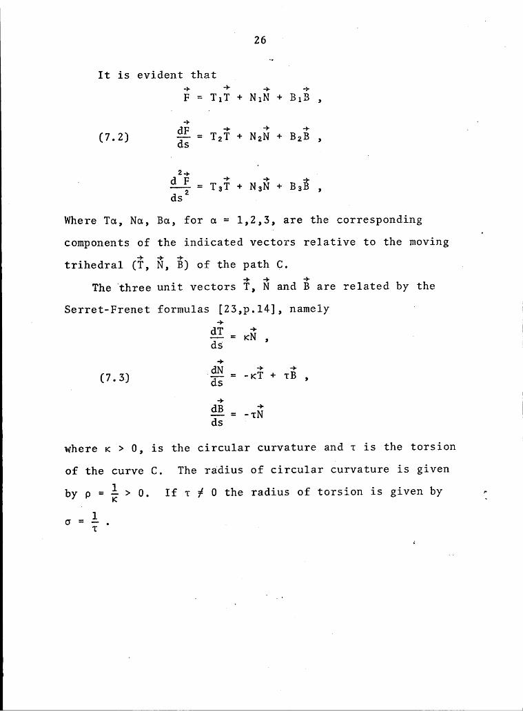
It is evident that C+ "* + —>F=T1T+N1N+B1B,

dp -> + ->· .(7.2) ——— = TZT + NZN + B2B ,ds

~ dz? ‘*.·* +7

•-—é-=T3T+N3N+B3B ,C ds _

Where Ta, Na, Bd, for a = 1,2,3, are the corresponding

components of the indicated vectors relative to the movingI

trihedral (T, W, B) of the path C. 7

The three unit vectors T, Ü and B are related by the

Serret-Frenet formulas [Z3,p.l4], namely C ·‘ +

Q1 = Kg ·ds ’

di; -> +(7.3) ‘ä; = -KT + TB ,

A+

dB *....: • Nds ·T

where K > 0, is the circular curvature and T is the torsion

of the curve C. The radius of circular curvature is given

by p = é > O. If T # 0 the radius of torsion is given by T

o = . „r

7 l27

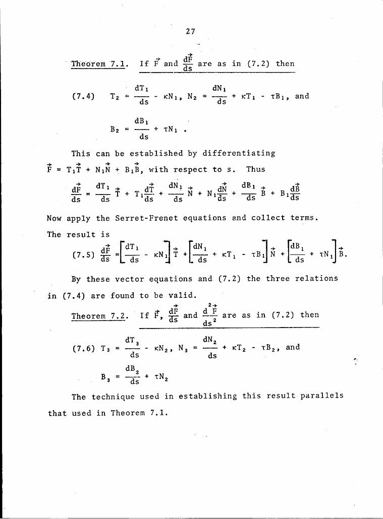
'°Theorem 7.1. If F and E; are as in (7-2) then °

T2 = ·•——·• " KN}, N2 = ———·-— + KT} · TB}, Hfld~ ds ds _

_ B2 = -—-—— + TN} .. ds

. This can be established by differentiating+ ·) ·+ +F = TIT + NIN + BIB, with respect to s. Thus

.§.i:=........dT1i‘)+T§.:i+.......dNliq>+N.€1Ä\I*.+.-.dB1-§+B§.§.7 ds ds lds ds lds ds lds

Now apply the Serret—Frenet equations and collect terms.

_ » The result isa·§=·—··ä·§" KN} T+·•"·dT§·+KTl *‘ TB}N+···ä·§+ TN]. B,

I By these vector equations and (7.2) the three relationsv

in (7.4) are found to be valid. '—> d2—>·

Theorem 7.2. If F, gg and -Ȥ-are as in (7.2) thends

dT3 dN2(7.6) T3 = —-— - KN2, N3 = ——— + KT, - TBZ, and

ds dg . LdB2 ‘

. ~ B3 = + TN2

The technique used in establishing this result parallels

that used in Theorem 7.1.

T28

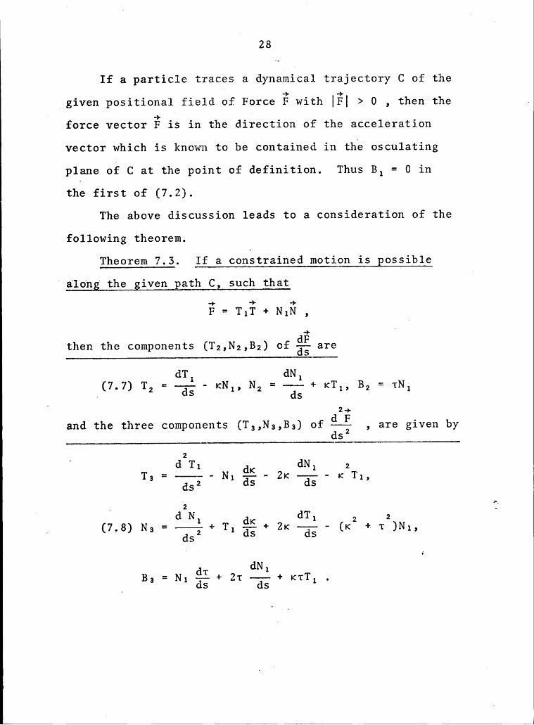
If a particle traces a dynamical trajectory C of the

ggiven positional field of Force with [Bl > 0 , then theT

force vector B is in the direction of the acceleration

vector which is known to be contained in the osculating

plane of C at the point of definition. Thus B, = 0 in

the first of (7.2).

The above discussion leads to a consideration of the

following theorem.Theorem 7.3. If a constrained motion is possible

"along the given path C, such thatC

F = TIT + NIN , I

then the components (T2,N2,B2) of gg are

dT1 dN,T2 = —ä; - KNI, N2 = —ä; + KT,, B2 = TN,

2+and the three components (T,,N3,B3) of E-; , are given by

s

' d2T dN

_ . 2Y T_, (7.8) N3 = ggg; + TI gg + ZK fg; — (K2 + r2)NI,

B3 = NI gg + 2r gg; + KTT1 .

' 29 7

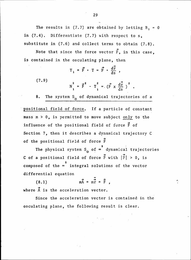
The results in (7.7) are obtained by letting B, = 0 ‘C

in (7.4). Differentiate (7.7) with respect to s,

substitute in (7.6) and collect terms to obtain (7.8).Note that since the force vector F, in this case,

is contained in the osculating plane, then

2 +2 2 + d; 2N1 = F — T1 =.(F x E; ) .‘ ( 8. The system S0 of dynamical trajectories of a ‘

'positional field of force. If a particle of constantmass m > 0, is permitted to move subject only to the-

influence of the positional field of force F ofSection 7, then it describes a dynamical trajectory Cof the positional field of force F

The physical system SO ofws

dynamical trajectoriesC of a positional field of force F with [FI > 0, iscomposed of the

wsintegral solutions of the vector

differential equation(8.1) mK=m?=?, in

where Ä is the acceleration vector.

Since the acceleration vector is contained in theosculating plane, the following result is clear.

Ie

30

i'Theorem 8.1. The physical system SO of the ws

)‘dynamical’trajectories’of a positipnal field offorce’with°[F[’>°0,°is‘givenby the system of equations '

F = TIT + NIN.,

dv.....=T:F•..„...(8.2)‘“"aS 1 ds,

mv2 +2 4- df 211/2 W

-—;—-=N1?$[F-(F·ä;) „

where 6 is either +1 or -1. 3For this situation, the T3, N3, B2; T3, N3, B3; of

(Section 7, can be evaluated by obtaining the space

derivatives of TI and NI . The procedure is similar to

that used by DeCicco in [22]. Thus‘

ÖT1 2 2_ d v dv. —ä; m[V ds, + ( ds ) 1(8.3)

dN1 2——— = m[2vK Q! + v Qi ] .ds ds ds

The next step is to substitute these results into the „

expressions for T2, N3, B3; T3, N3, B3; given in Theorem

7.3 to obtain I

1 131

d2 dT2=m[v-C—i—§‘-2,;-+(E1—;—.]z—vzKz] ,d C d 1

2 . N2 = m[3vK E; ] , 2 2B2 = m vz K T ,

(8·4) 2 2dsa ds dsz ds ds

— 1 2N3 = m[4vK Q-E + 4K( Q! )z + Sv QX QE + vz éiä - (Kz+Tz)vzK] ,

dS2 ds ds ds dS2

21

B; = m[2vzT gg + 5vKT gg + VZKäé ] .

‘ Now consider two dynamical trajectories C; and C2

described by rl = rl (s) and respectively,

such that the two paths intersect at the point Po . Let

PO correspond to the values s = so and s* = sg on C, and C2,

respectively. Then, of

course,Thefollowing definition can be found in [27,pS0].

‘· 32U

' Definition 8Ll. A curve C, described by fl = ?1(s) ,

has contact of order n with a curve C_ described by+rz = ;2(s*) , at the point Po if y

-)·?,(sO) = r2(sg) = PO , for some so and sg , P T

(8.5), dkrl dk?2————— = —-——— , for l i k j n ,ask a(s*)k

= x: as so s so

and, if the derivatives of order (n+l) exist at PO, then

:: 7$:<‘

y s so s s ODefinition 8.2. A curve C has contact of order n

with a surface S at a point PO if there exists at leastone curve C* on S which has contact of order n with C and

there does not exist a curve on S which has contact of

order greater than n with C at PO.This definition is based on that found in [27,p5l].

The osculating plane to a curve C at a point PO is

known to have contact of the second order with C at the“

point PO, and second order contact is usually known as

osculation. Contact of order higher than two is called _

super osculation or hyper osculation. ‘

h33

9. °A°study of the curvature and the torsion of

°°a“dynamica1 trajectorv. In a positional field of force,

the force vector F acting at any point P of a dynamical

trajectory C, with K > 0 , at the point P is contained in

the osculating plane of the dynamical trajectory C at this

point P. Thus,+ + ->F = TIT + NIN , J J

where- 2

mv QX = TI and EX-= NI .ds p

This set of relations implies that formulas (8.4)

are applicable. From these it is found that—- x F = NIB = mv2KBds

(9.1) —a? —> dl?

J ( E; , F, E; ) = m2VkK2T . JA Theorem 9.1. The torsion 1 of any dynamical

trajectory C of a positional field of force F, with' |F| > O , is +df g dF

B(--.9 !'—~_)

. _ 2 ds dg(9-2) r=F=————=:—-——··————-—1 dr * 2 „... ap J( ds X )

. where NI is assumed to be not equal to zero.

From Theorem 7.3, it is found that B2 = TNI ,t

which gives the first part of the equality. The second I

ipart follows immediately from (9.1). 2

l

34' 1. . . ’dK

‘°Theorem 9.2. The rate of Variation, —— , of the———————————— _______„__________„„_„„._ds..........

Äcircular curvature K pg£_unit of arc length s along any. —>

"dynamical°trajectory C‘of a positional_field of force F

with |;| > O , is 1

(9 3) QE = Ji-[N — SKT ] ,’ ds N1 2 1

if N1 # 0 . 1In the dynamical case it is known that mv2K = N1 .

1 Differentiate this result with respect to s and solve

for és to obtain 1ds ~ · .1 -‘l'$='<[N-sw] 1

ds NT 2 1 ' ·

Using the definition of the radius of curvature(p = é ) , equation (9.3) can be written as

(9.4) N 92 = 3T — pN1

1 ds 1 2 ’

which is used to obtain the derivation of a theorem onrest trajectories originally stated and proved by Kasner.This will be discussed further in Section 10. „

. ‘35°

Theorem 9.3. The rate of Variation gg of the torsion°I'per‘unit°of arc length s'along°any dynamical trajectory C

‘of‘a'positional field of force with ]B| > 0 , is V

‘ (9 5) gl = éL [B — ZIN + IKT ]3

° ds N1 3 ” 2 1 ° 1

if N, f 0 . V

By differentiating I = -—·, with respect to the arcN1

length s of the dynamical trajectory C, it is found thatdB, dN1

„ N — Bdm _ 1 ds 2 ds(9.6) E; — ——————————-——-— VN21

· dB2 dN1Next, substitute the expressions for ——— and ——- ,ds ds

·\found in Theorems 7.2 and 7.3, into (9.6). ·“ Upon simplification, the formula (9.5) is obtained.

10. Rest trajectories.Definition 10.1. If a particle in a positional °

field of force starts from rest, the resulting path is[ termed a rest trajectory. „

A discussion of rest trajectories can be found in

[28].3 I

I _

The initial Velocity Vector for a rest trajectory C,

is the zero Vector. At the initial point of a rest

136

2

trajectory C, the force vector is tangent to the

trajectory. Thus, the initial conditions for a rest

trajectory are ° i

N1 = O , _(10.1) K _ 1 2 N2

D STI *

where it is assumed that gg is ngt perpendicular to N so

that T1 # 0 , and N2 ä 0 .2

The Faraday lines of force of a positional field of

force with [R] > 0 , (Chapter I) consists of the @2

solutions of the vector differential equation 1 -

2 (10.2) gä = aF ,

where d is a non-zero scalar.

_ Thus, it is noted that a rest trajectory and a Faraday

2 line of force have a common unit tangent vector at the

p initial point of the rest trajectory. That is] they have

contact of at least order one at the initial point of the

rest trajectory.

The following result is known as Kasner's Theorem onI

Rest Trajectories and can be found in [9].

.” 37

I

°°Theorem;lQIl. The ratio of_the curvature of a rest0

'°trajectory to that of the correspgpding Faraday line of

° force at the initial point, is‘1/3,'provided'that‘the I

°°order of contact is exactly one. .

From equation (10.2) for·the system of @2 Faraday

lines of force it is noted that4+ + + 1/2i +

~ (10.3) F = (F•F) 1 = TIT

where T is a unit vector in the direction of F. Now T is

_ tangent to the Faraday line of force and the rest

trajectory with initial point at the point in question.

— Differentiate (10.3) with respect to arc length of

the line of force to obtain

ggwhere<* is the curvature and N* is the principal normal

to the Faraday line of force.

The first derivative of the force vector F with 1

respect to the arc length s of a dynamical trajectory is

Igivenby. I

T6? + + —> h= TIT + NIN + BIB ,

where T, N, and B are the unit tangent vector, unit hormal

vector and unit principal vector, respectively.

38If

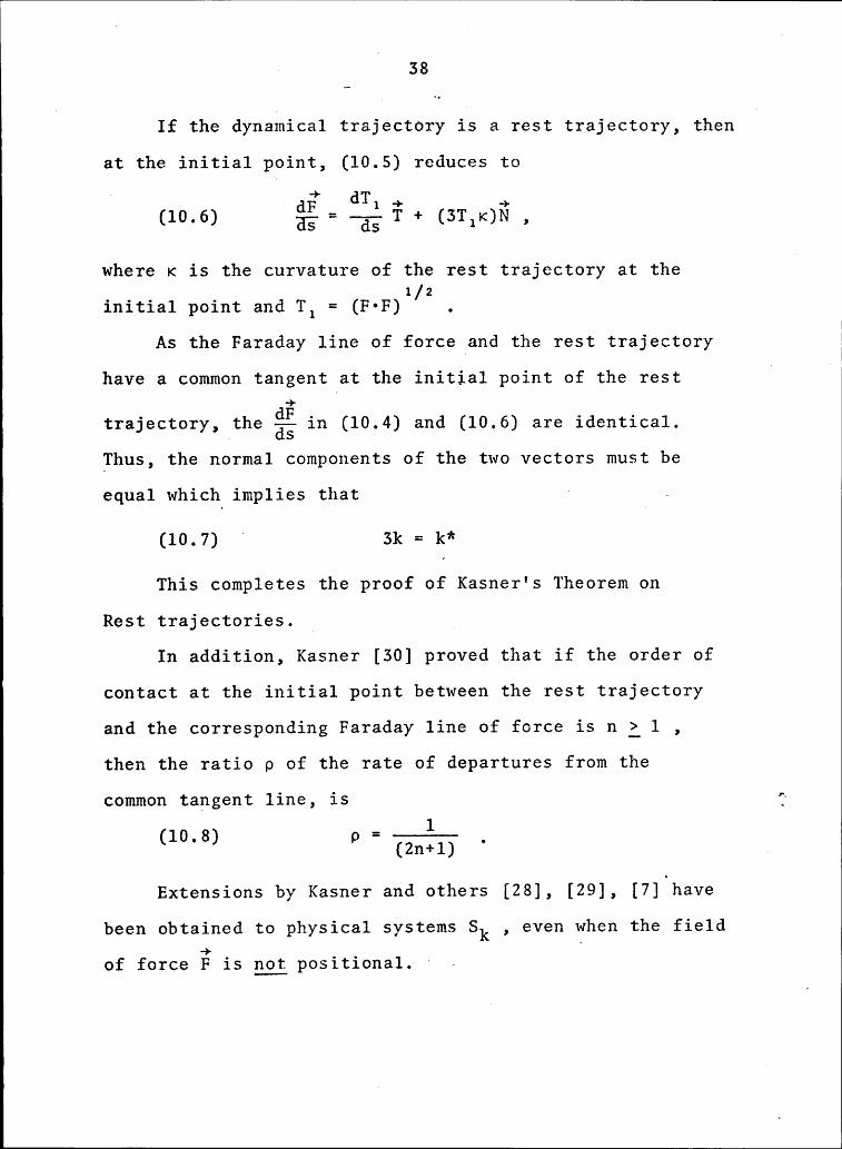
the dynamical trajectory is a rest trajectory,thenat

the initial point, (10.5) reduces to[ C11? TÖT1 —> + 6

(10.6) ·a§ = —ä§ T + (3T1K)N ,

2 where K is the curvature of the rest trajectory at the[

' 1 2initial point and T1 = (F•F) / .

1As the Faraday line of force and the rest trajectory

have a common tangent at the initial point of therest·->

trajectory, the gg in (10.4) and (10.6) are identical.

Thus, the normal components of the two vectors must be

equal which implies that ( .

(10.7) ‘ 3k = k*

This completes the proof of Kasner's Theorem on

Rest trajectories. AIn addition, Kasner [30] proved that if the order of

contact at the initial point between the rest trajectory

and the corresponding Faraday line of force is n 1 l ,

then the ratio p of the rate of departures from the

common tangent line, is il10.8 = —————— _( ) p

(2n+1)

Extensions by Kasner and others [28], [29], [7] have

been obtained to physical systems Sk , even when the field

of force E is not positional. ‘ -

CHAPTER IV

..HALPHENVS.THEOREM AND SOME RHlATED.RESULTS.IN.E3 .

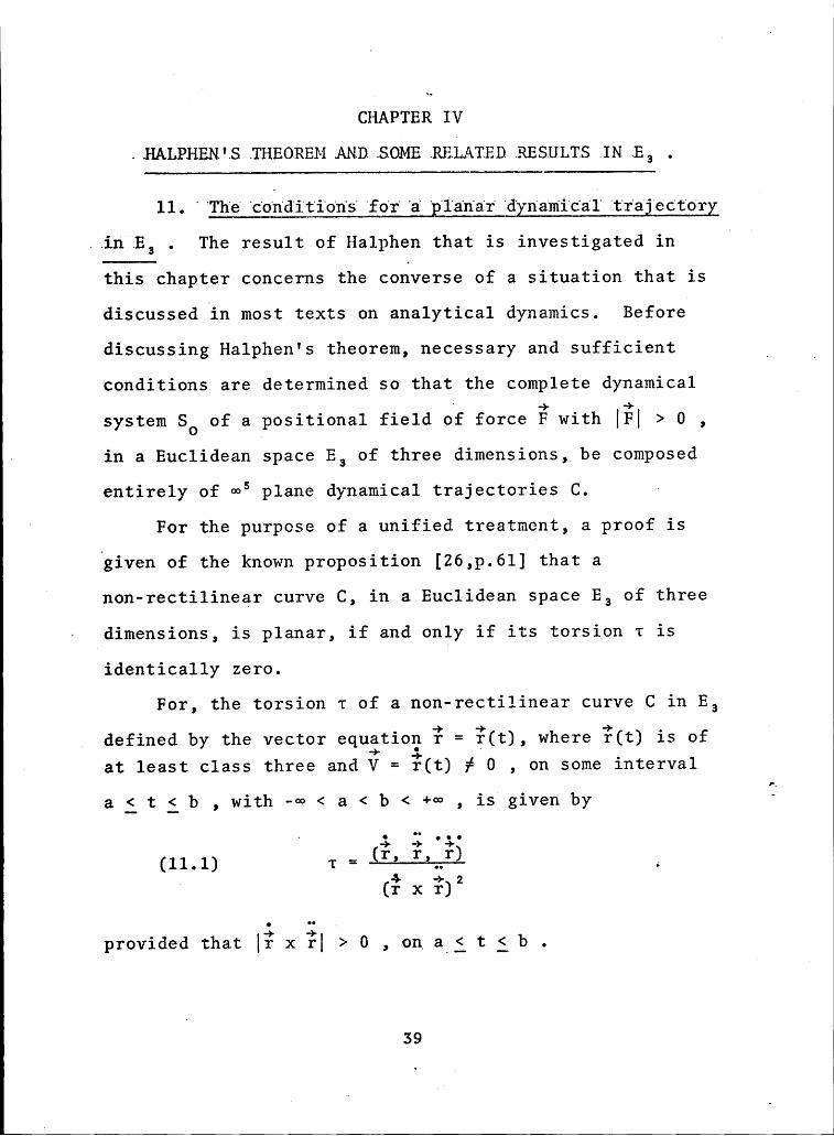
11."The°conditions;jQE;g;p1anar’dynamical°trajectory..in E, . The result of Halphen that is investigated in

l

this_chapter concerns the converse of a situation that is

discussed in most texts on analytical dynamics. Before

discussing Halphen's theorem, necessary and sufficient _ Vconditions are determined so that the completedynamicalsystem

S0 ofva positional field of force with |;| > O ,B in a Euclidean space E3 of three dimensions, be composed

entirely of ws plane dynamical trajectories C. ·( For the purpose of a unified treatment, a proof is

sgiven of the known proposition [26,p.6l] that a

non-rectilinear curve C, in a Euclidean space E3 of three— dimensions, is planar, if and only if its torsion 1 is

identically zero.For, the torsion 1 of a non-rectilinear curve C in E3

C defined by the vector equation = ¥(t), where r(t) is ofat least class three and V = %(t)

#·0, on some interval

a ipt i b , with -w < a < b < +w , is given by T

(11.1)s

1providedthat x‘?| > 0 , on a_j t i b .

l39

”' 40

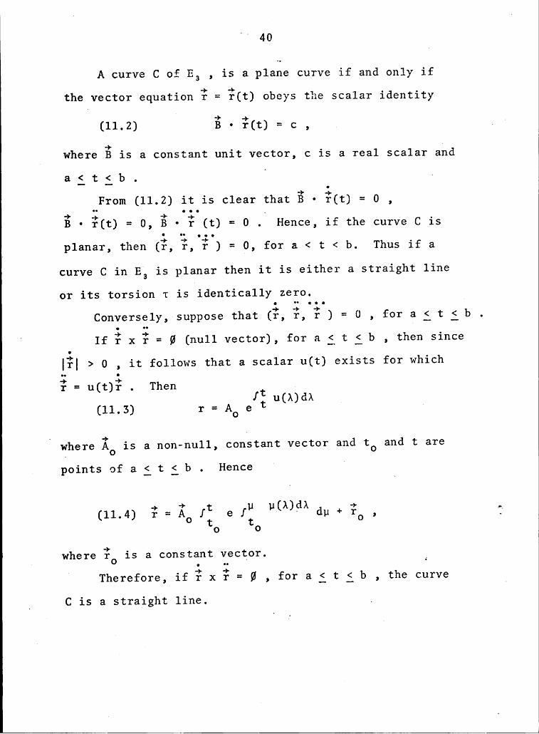
A curve C of E3 , is a plane curve if and only if

the vector equation = r(t) obeys the scalar identity

(11.2) B • r(t) = c , „ ‘

Y where B is a constant unit vector, c is a real scalar and

a j t i b . · —

From (11.2) it is clear that B • r(t) = 0 ,-* ; +

•;• _·B • r(t) = O, B • r (t) = 0 . Hence, if the curve C is

planar, then (r, r, r ) = O, for a < t < b. Thus if a

curve C in E5 is planar then it is either a straight line

or its torsion 1 is identically zero.

Conversely, suppose that (r, r, r ) = O , for a i t i b .( If r x r = 0 (null vector), for a i t i b , then since

I?] > 0 , it follows that a scalar u(t) exists for which

r = u(t)r . Then Bxt u(A)dA(11.3) r=1-106 t 3

B where Ko is a non-null, constant vector and to and t arepoints of a i t i b . Hence 1 (

A dl 1(11.4) r = K ft e fu u( )· du + , T

O t t O0 O

+ .where ro is a constant vector. _Therefore, if r x = ß , for a i t i b , the curve

_ C is a straight line. .

. L 41

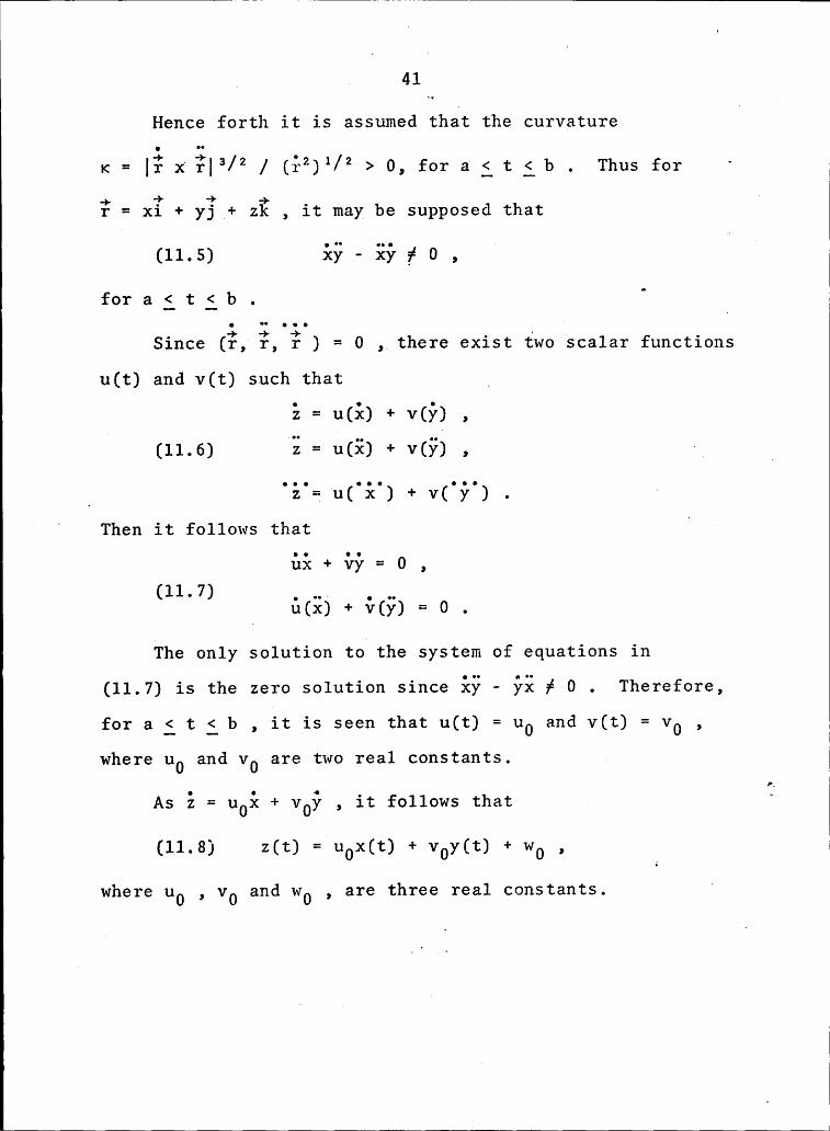
Hence forth it is assumed that the curvature1

•<= |¥xi·’|3/2 1 >0, for azitib. rhus fer ·—> *1* 1* —> _ ·r = X1 + YJ.+ zk , lt may be supposed that

(11.5) - iii--; 0 , ‘

for a i t i b . °

, L ll °L° _ ~ ”S1DC6 (r, r, r ) = 0 , there exist two scalar functions

u(t) and v(t) such that _

Iz = ¤(50 + vciz) ,(11.6)

72= u(§) + v(y) , ·_

·

. 'ä°z *¤C°$<'J + vc°$«°) . (' Then it follows that

I

ui + yy = 0 ,(11-7) . , ..¤(><) + v(>') =0Theonly solution to the system of equations in

(11.7) is the zero solution since iy - yä # 0 . Therefore,

for a i t i b , it is seen that u(t) = uo and v(t) = vo ,

where uo and vo are two real constants. zAs E = uoi + vüy , it follows that z L

( (11.8) z(t) = u0x(t) + vOy(t) + wo ,

where uo , vo and wo , are three real constants. ‘

’ Consequently, if Is x §|_> D., and (%,‘%, fs) = 0_, ifor a i t i b . The path is not straight and is a plane

curve C in E,.” r ”

An expression for the torsion 1 of a dynamical ‘

trajectory C , in terms of the space derivatives of the

force vector of a positional field of force was given

in (9.2). Thus, the following result is clear.‘ Theorem 11.1. A dynamical trajectory C, given by the

vector eguation ? = ?(s) , with s representing arc length,

in a positional field of force F with |F| > 0 , in E, is

· planar if and only ifU

(11.9) (%;l,i=s,ä-§)=0, Vis a scalar identity.

‘ Tp In addition, this scalar equation, if not an identity,

defines the tangent directions at an admissible point p, °

such that if a particle starts from such a point p in

anyone of these tangent directions, then it describes a

dynamical trajectory C that is initially fläf (t=O) at the j

_given point p .12. Halphen's Theorem. In most texts on analytical

dynamics, it is shown that the ws dynamical trajectories C,

of a parallel or central positional field of force in E3

43 _

are all plane curves. The converse result is not as well

known but it is also true. p. °

A new proof of this converse result is presented in T

the following theorem which is known as Halphen's Theorem

[31].‘

Theorem 12.1. Every dynamical trajectory C of a

'positional field of force F with |;| > 0 , in Euclideany space E3 of three dimensions, is planar, if and only if

the positional field of force is either parallel or central.The force vector F acting at any admissible point is .

(12.1)wherethe three cartesian components (¢,w and X) are such

that lg! = (¢2 + W2 +_ x2)‘/2 > 0-· If a dynamical trajectory C is defined by the pair of

explicit equations y = y(x) and z = z(x) , then it is a' plane curve C if and only if

1 y' z'(12-2) W W xi = O ,¢>• w' x' T ‘where the primes denote total differentiations with respect

to x. T ‘

44U

Upon expanding the determinant and simplifying, the

preceding is equivalent to the equationW

a(y')2 + 2by' z' + c(z')2 + 2dy' + ”

(12.3) 2_ + 2ez' + f = 0 ,

where¢ay,

-.-1 EE- E2; EE-E¢C

W öz W öz ’ ‘ °

(12.4) 1 34 y=.. ..9;- E2; E2;- EE

E -1 EE- EE E2;- MLe 2 ( W öx W öx + W 32 X öz ) ’

f W 8x. X öx 'W

If the ws dynamical trajectories of a positional field

of force g with Igl > 0 are plane curves, then the equation

(12.3) is an identity. This is equivalent to saying that

each one of the six coefficients a, b, c, d, e, f is

identically zero, and conversely. USince |;| > 0 , there is no loss in generality in

_

assuming that ¢ = ¢(x,y,z) # O .

p Under this supposition, the two slope functions; _a = a(x,y,z) , B = B(x,y,z) , of the positional field of

l

.I

45 .

force F = ¢i + wj + Xk , are defined by

s2. E °(1 5) X = B¢ • l

Then the system of six equations in (12.4) becomes

the set · -l -_ 2BBb

Z [ az + ay Ä ·G

(12.6) 2= Q. -EE EE - EQE d2

[ Gx + G Gy B Gy ]'

'

E _ ¢2 aa aß _ Gu. 6-·····ä[•ä··5<··+(Y„·ä··Zf

= ¢2[¤ gg - B gg ] .

Evidently, a = 0 and c = O , if and only ifE

¤ = ¤(X„Y) ,

Then a = 0 , b =.O and c = 0 if and only if

¤ = m(x)y + u(x) ,B = m(x)z +

VCX)wherem(x) , u(x) and v(x) depend only on x .Hence the three functions, d, e and f , of (12.6)

assume the farms _

46

d=-%[(䧗+m2)z+ (ä-;’§+mv)]

(12.9) 6 6 m2)y my]_ 2 Y dv “du ‘ 6

f *• $[7.1 Hi " V Hi]•

These three expressions are identically zero if andonly ifi 4ää + m = O ,

(12 10) du + mu =’0•‘ Ei ,‘ I 4

ää + mv = 0 .'

4

A If m(x) = 0 , then u and v are two constants.°. This means that a = ao , B ä B0 , are two real constants.

The corresponding positional field of force g with

~[gl > 0 , is parallel. ·

_

lIf m(x) # 0 , then the solution of (12.10) is

]ll(X) ·

. Y6 (12-ll) UCX) =·;··;·Q·g·6· »

0

V(X]wherexo, yo, 20 are three real constants. ‘

Therefore, (12.8) assumes the form

i47

DB=3··(··j··—f%, A_ n lwhere xo, yo, 20, are three realconstants.Thus,

the corresponding positional field offorcewith|;| > O , is central with center at P(x0,y0,20) .·

Consequently the proof of Halphen's Theorem isn

y completed.I

The following sections contain new results related to

Halphen'sTheorem.l3.„The notion of a flat point of a positional field

of force E3 . Consider a positional field of force

H = ¢i + wi + xi , r°A with |;| = (¢2 + wz + X2)‘/2 > 0 , of at least class two,

Ddefined on a certain open region of a Euclidean space E3

of three dimensions. i

Definition 13.1. A flat point P(x,y,z) is in the

_given region, and is such that every dynamical rptrajectory C of the given positional field of force H ,

D

has contact of at least order three with its osculating

plane H constructed at the given point P(x,y,2) .” .

( A48

I I

Thus, a point P(x,y,z) of a_given positional field

of force g with [gl > Ö , is flat and only if the equation

(13.1) (Wg.? ,ä—§) =i0,

is an identity in gg = i gg + äé + gg , yT at the point P(x,y,z) .

Theorem 13.1. A point P(x,y,z) of a positional field

of force g = ¢i + mj + Xi , with ¢ f O , is flat if and only

.if the two slope functions d = , and B = é , obey the

set of five eguations

-gg-=o,-gig--§%=o,§"i=o,(13.2) _

%S%·*¤%%=°.··ä·?z+ß%·€·=¤·at thepointFor,

by the two set of equations (12.3) and (12.4),‘

‘ ( a point P(x,y,z) of the given positional field of force

; with ¢ # O , is flat, if and only if a = 0 , b = O ,

c = 0 , d = 0 , e = 0 and f = 0 , at the point P(x,y,z).

This set of six conditions is seen to be equivalent T

to the system of five conditions listed in (13.2).

According to Halphen's Theorem, a positional field

of force g with I;] > O , is either central or parallel,

‘ 49i A I

if and only if every one of its points P(x,y,z) is flat.i

"Theorem°l3.2. g_point P(x;y?z)'0f a positional

°°field'of°force'P°='¢i°¥ w§°¥°X§ g with ¢ # 0 2 is flat i

°’if and only if there exist six distinct directions passing( through P , and these directions are not all on a common

guadric cone Q with vertex at the given point P(x,y!z)_y

such that the corresponding dynamical trajectories C passing° through the point P(x[y,z) in each of these six directions' is hyperosculated by its osculating plane H constructed at

the given point Pgx,yzz) . Q_ If the point P(x,y,z) is a flat point of the positional

field of force P , then every dynamical trajectory C passing

through P(x,y,z) is hyperosculated by its osculating plane H

at the point P(x,y,z) .l 4

If there exist six distinct directions (1,y',z')

passing through the given point P such that they do not all

lie on a quadric cone Q with vertex at the given point P ,

and such that the corresponding dynamical trajectory C

passing through the point P(x,y,z) in every one of the six

directions is hyperosculated by its osculating plane H at T

the point P(x,y,z) , then the directions (l,y',z') satisfy

equation (12.3) . This results in six equations inifive _

essential unknowns. Since these six directions are not on

the same quadric cone Q with vertex at P(x,y,z) , then the

six unknowns a, b, c, d, e and f are identically zero at

‘ 50

the_given point. Thus, the point P(x,y,z) is a flat point

of the positional field of force.

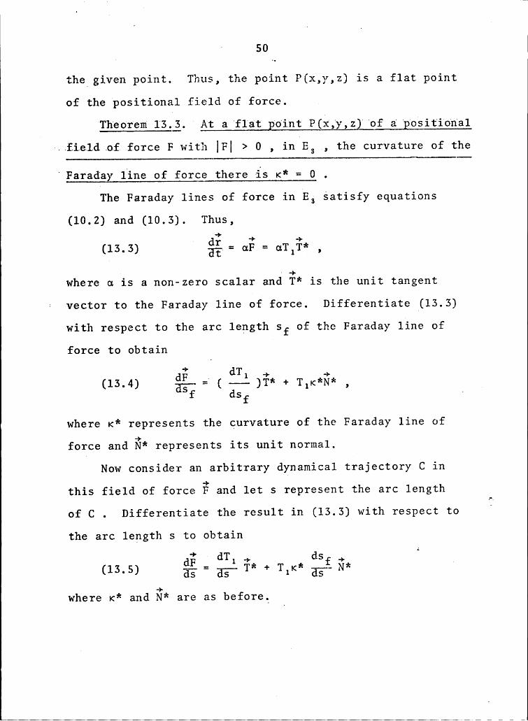
‘Theorem l3¥3.° At a flat point P(X.y,z)'of a°positiona1

„.fie1d.of force F with |F| > 0 , in E3., the curvature of the

°‘Faraday line of force there is K* = 0 .

lhe Faraday lines of force in E3 satisfy equations

(10.2) and (10.3). Thus,

(13.3) N =¤1_?=

ovrlié ,

where d is a non-zero scalar and ¥* is the unit tangent

» vector to the Faraday line of force. Differentiate (13.3)

with respect to the arc length sf of the Faraday line of

force to obtain(

(13.4) H§— = ( ——— )T* + T1K*N* ,f dsf ·

where K* represents the curvature of the Faraday line of '

force and N* represents its unit normal.(Now consider an arbitrary dynamical trajectory C in

this field of force g and let s represent the arc length

of C . Differentiate the result in (13.3) with respect to T

the arc length s to obtain

(13.5) gg = ääi l* + T1K* äéi N* '

where K* and N* are as before.

51

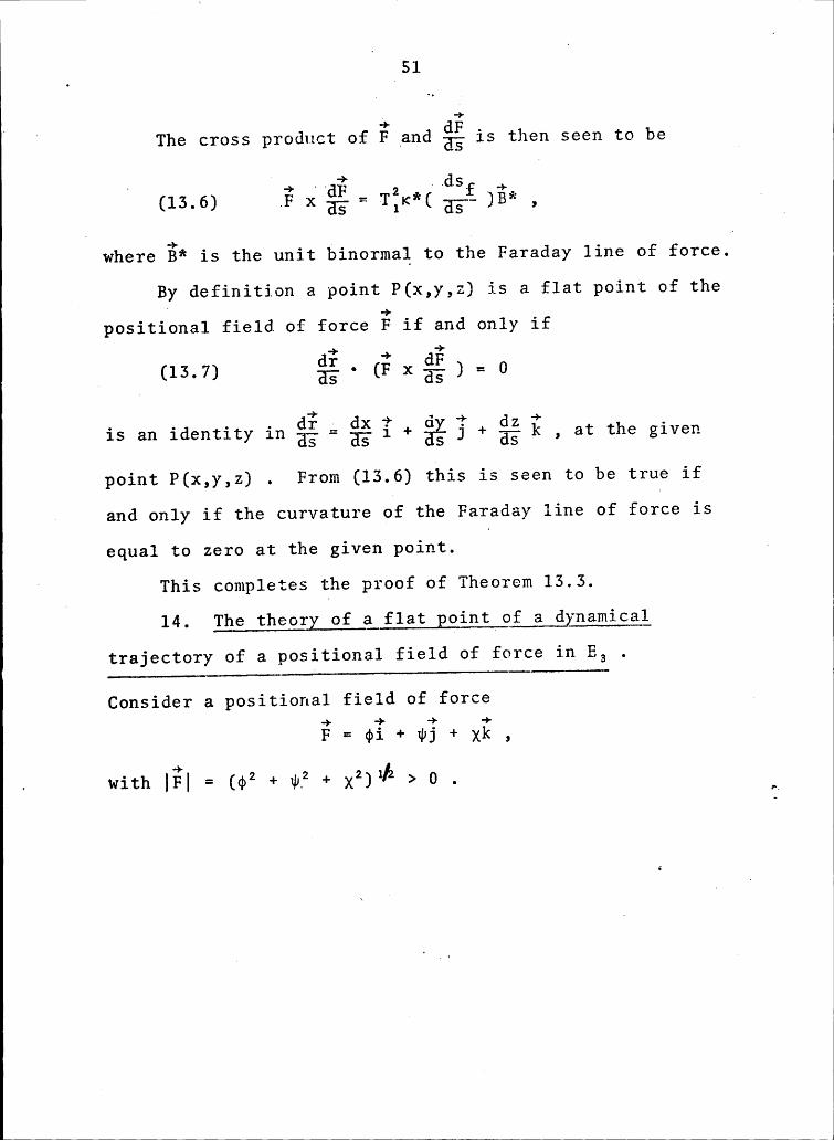
The cross product of F and ag 15 then seen to be

. ’ .. + ..dsr dF _ 2 f *(13.6) .F x E; ~ T1r*( E§~ )B* , g

where B* is the unit binormal to the Faraday line of force.

By definition a point P(x,y,z) is a flat point of the

positional field of force F if and only if—> _) ·>

(13.7) ä—§•(Fx—ä§)=0

+ .is an identity in S; # ää i + ää + gg , at the given

point P(x,y,z) . From (13.6) this is seen to be true if

and only if the curvature of the Faraday line of force is

equal to zero at the given point. ~

( This completes the proof of Theorem 13.3.

14. The theory of a flat point of a dynamical

trajectory of a positional field of force in E3 .

Consider a positional field of force-) —?· + ·+F=¢l+‘Pj+Xk 0

„ with |§| = (02 + 02 + Xw/2 > 0 . rg

( · 52

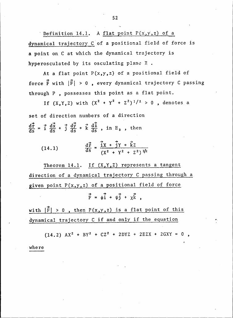
° Definition 14.1. A flat point P(x2y,z) of a

dynamical trajectory_Qgof a positional field of force is

a point on C at which the dynamical trajectory is

hyperosculated by its osculating plane H .

At a flat point P(x,y,z) of a positional field of

force P with |P| > 0 , every dynamical trajectory C passing

through P , possesses this point as a flat point. ·

If (X,Y,Z) with (X2 + Y2 + Z2)1/2 > 0 , denotes a

set of direction numbers of a direction-> + —)- _ +

E

ää = i ää + g gg + gg , in E3 , then_} —> —> 4

n

y dr _ iX + jY + kZ(14.1) H; - ————— —l ~ (X2 + Y2 + Z2)1/2

Theorem 14.1. If (X!Y,Z) represents a tangent

direction of a dynamical trajectory C_passing through aI

(given point P(x,y,z)_of a positional field of force

+ j> —+‘ F = ¢1 + wa + xk ,

with |P| > 0 , then P(x!y,z) is a flat point of this

_ ° dynamical trajectory C if and only if the equation ‘ „

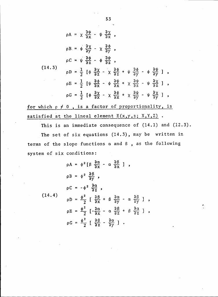
(14.2) AX2 + BY2 + CZ2 + ZDYZ + ZEZX + 2GXY = 0 ,

—where

53

¤A x ax w ax „

= °äl - B22¤B— 4 ay x ay „ _

= ·“22 -dä!pc V az V az ·

‘(14.3) 1 .= .. El - 22 EQ - 22

¤E=·g[¢gg·B¢—gg+xgg-wggl,V oG = g [¢ gg — x gg + x gg — w gg ] ,

for which p % 0 , is a factor of grogortionality, is B

satisfied at the lineal element E(x,yL£i_},Y,Z) .B

This is an immediate consequence of (14.1) and (12.3).B

_The set of six equations (14.3), may be written in

terms of the slope functions d and B , as the following

system of six conditions: _ (

‘ B: 2.§..§.l o 4 ay „ M

¤C = ·¢’ gg ,2 •\

= Q. zä E9 - EE-13. -214.-aa*°E ’ z [ ax V az + B az 1 ·-¢i é.ß.-.¢;1°B “ ‘g [ az ay ] · _

I

· ,54 ä°Theorem”l4;2. At a non5flat point P(x,v,z[ of a

g.

‘°the'tangent‘directions°(X,Y,Z)'of°all possible dynamical

"trajectories C passing_through the point P(x,y,z) and T

°°having a flat point at P(x,y,z) , describe a quadric cone Q

'with vertex at P(x,y,z). .

The quadric cone Q , is described by equation (14.2).’ The next theorem is important in that it represents a

less restrictive form of Halphen's Theorem.4 Theorem 14.3. A positional field gf_fgyce P with

[PI >°0 , is either central or parallel if and only if_a£every point P of the region of definition there exist§_atleast six distinct directions, not all of which are on thesame guadric cone with vertex at P , such that the dynamical

_ trajectories C passing through P in each of these six

directions have P as a flat_point.· If the field of force is either central or parallel,

then this result is trivially true since every point on a

dynamical trajectory C in such a field is a flat point of

the dynamical trajectory C. I T

The converse follows by appealing to Theorem 13.2 to

find that every point P in the region of definition is a

flat point of the positional field of force. Thus every

·

55dynamicaltrajectory in such a field is planar and the

field of force is either central or parallelr15. ‘A'study’gfythe‘quadric°cgggyQ_gf‘Theorem 14;;. 0

The characteristic equation of the quadric cone Q ,

represented by (14.2), is .(

. A-p G E _ ~° (15.1) G B-p D = O

‘ . E D C-p

This characteristic equation is a cubic in p ,

namely,(15„2)p2 - Ipz + Jp - A = 0 , ·

where the three invariants I, J and A are

I a A + B + C·(15.3) J = BC + CA +

AB'- D2 -‘E2- G2

A = ABC - AD2 - 662 + 2E06 - BE2 .The quadric Q represented by (14.2) has centers of

symmetry and is homogeneous in X, Y and Z . Thus, itsreduced canonical form is given by

iälpi zi = 0 ,

with 1 i r i 3 . The following is taken from [15]. T

Theorem 15.1. 1jyl_j_0, J = 0 , and A = O , thenthe guadric Q described by (14.2) is comgpsed of two‘ ‘

identical planes n passing through the point P(x,yLz).l

WW

” 56 1

. [If I #_O , J =-G and A = 0 in (14.2) , it is

~

apparent that two of the eharacteristic roots are zero. “

Thus, the rank of the coefficient matrix of (14.2) is one.

.The result then follows by appealing to the reduced Q(

canonical form. _1

‘Theorem 15.2, If J # O and A = 0 , then·the quadricU

°Q°described bx (hihäl is comhosed of two distinch'intersecting Qlanes or a single line gassing through"F(x,X,z).

Under the conditions of the hypothesis, it is notedthat the rank of the coefficient matrix is two. The °

conclusion is then a consequence of the reduced canonical

form knowing that r = 2 .1 Theorem 15.3. 1£_h_j_p , the quadric cone Q of (14.2)

is a non degenerate quadric cone Q . The quadric cone Q is

real or imaginary depending on the signs of the pa for

a = 1,2,3 .If A # 0 , the rank of the coefficient matrix of the

quadric Q represented by (14.2) is three. Thus r = 3 in

the reduced canonical form and the result is obvious. T

If A ä 0 and the roots of (14.2) are not of the same

sign then the quadric Q is a non·degenerate, real quadric

U 57 r

cone Q . This quadric cone Q is right circular if andl

only if the characteristic equation (15.1) has a double

root. The quadric cone Q is elliptic if and only if the

characteristic equation (15.1) does not have repeated roots.

Theorem 15.4. If_P(x!yéz) is not a flat point of the

positional field of force F with |F| > 0 , and A # O then‘the°related guadric cone Q of (14.2)z is rectangular if

'and only if __—)· —>

· (15.4) F • (V x F) = O ,

at the point P(x,y,z) . UIf the force vector F is represented by

:F*=¢}+¤l»i+x§„Wi’¤h(¢2+¤P2+><2)‘/“>0,’¢h@¤,+• Ü:VX}T

By rearranging terms and using equation (14.3) it is

found thatA

- + -)·U (15.6) F • V x F =_p(A + B + C) ,

where p # 0 , is the constant of proportionality in (14.3). F

Thus, the inner product of the force vector F and the

curl V x F , is equal to a constant times the trace of the

coefficient matrix of the related quadric Q described by

(14.2). U"

S8

The conclusion then follows directly from [2lQp.l27];

It is also found that if the quadric Q in (14rZ) is

rectangularQ then at least one of the_generators of the Q

asymptotic quadric cone P has Qas./EGG

direction cosines, where the angles are measured from theQ principal axes of the quadric Q .

1 CHAPTER V

°'SOME°RBSULT§'CONCERNl§§ HELICAL2 . TRAJECTORIES IN E3

16. .The.theory.0f.helices.in.a.Euclidean,space E3 ,

The next definition is found in [25,p.l06]. _

°‘Definition_lQLl. A helix H is a curve of at leastclass three, whose tangent makes a constant angle with afixed direction.

U·

Let A represent a unit vector in the fixed directionand T represent the unit tangent vector to the helix H.

i 'U

Then by definition .

(16.1)U

T • A = cos Q ,

where Q is a constant.If the curvature K is not zero, then clearly H • A = O

and A is in the plane (rectifying) defined by T abd E .

This, along with (16.1), implies that” (16.2) A = (cos Q)T + (sin Q)B .

Differentiate this result with respect to the arc „

(length s. The result isT

_ (16.3) 0 = (K cos Q - 1 sin Q)§ . ‘

59

.60

·This implies thatU

(16.4) T/K = cot d = constant.

g - Therefore it has been shown that (16.4) is a ‘

necessary condition for a curve to be a helix. This leads

to the following well known proposition.(‘Theorem 16.1. g_gp£Xg_H”gf at least class three in_a1

..Euclidean space E! of three dimensions, is a helix if and

°only if it is either a straight line or else! when K ä_Q_!

(16.5) t/K = cot d ,I

‘where a is a given constant anglg. 1 A

In the case where H is a straight line (K = 0) thel

result is clear. Henceforth suppose that the curve H is

not a straight line (K #0)·.

Then by equations (16.1) through (16.4) the result

listed in (16.5) is found to be a necessary condition for

a curve H to be a helix.· Next consider the sufficiency part of the theorem.

‘ lf H is a straight line then it is a helix. „U

Henceforth assume that K # O and that t/K = cot a ,

where d is a constant.

61

Since r sin d = K cos d , it is seen that. +; . · +

( WW (16.6) (—rN)s1n a + (KN)cos m = 0 .

From the Serret—Frenet formulas in (7.3) of SectionU

7; it is noted that the above equation can be written as( ai aiS (16.7) E; (sin a) + H; (cos a) = 0 . _

Hence.z—>_ —> ' —>

_

_ B($1H a) + T cos o = A ,+ . .where A 1S a constant unit vector.

A Since T • A = cos a , it follows that the curve His.

a helix. pThe next theorem is an exercise in [23].

”Theorem 16.2. Aucurve iwi i(t)·of at least class four

in a Buclidean space E3 of three dimensions is a helix if

and 0nlX if

. dz da d“(16.8) (-—-il,-—§,—-f}i)=o.

ds ds ds

I

62

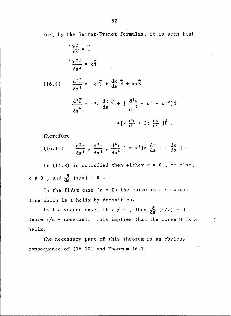
For, by the Serret—Frenet formulas, it is seen that‘_as"?'

...2*é...E;.,<§dsz T ·

(16.9) ggg = —K2T + gg H + Kt;·

¤+'* 2-3Kggq

ds 2ds ds

+[K gg + 21 gg ]§ .Therefore .

‘ dzr dar d“r _ 3 dt dK(ä—S:··é·,;1·;·;,ä·;;)—VK[Ka·§“TH§].

If (16.8) is satisfied then either K = 0 , or else,

d = · T TK # 0 , and HE (t/K) 0 .

In the first case (K = 0) the curve is a straight

line which is a helix by definition.In the second case, if K ¢ 0 , then äg (T/K) = 0 .

{ Hence t/K = constant. This implies that the curve H is a {helix.

The necessary part of this theorem is an obvious

consequence of (16.10) and Theorem 16.1.‘

( [63 E I U

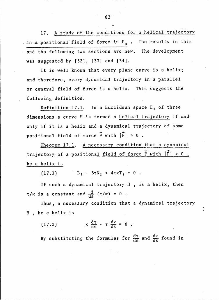
17. A study of_the conditions foy_ayhg1ical)tra]ectory

.in a positional field of force in E3 . The results in this3 and the followihg two sections are new. The development

was suggested by [32], [33] and [34].

. It is well known that every plane curve is a helixg ”

and therefore, every dynamical trajectory in a parallel

or central field of force is a helix. This suggests the

Ü following definition. 3 Ü ,Definition 17.1. In a Euclidean space E3 of three

dimensions a curve H is termed a hglical trajectory if andonly if it is a helix and a dynamical trajectory of some

positional field of force E with |E| > O .Ü

Theorem 17.1. A necessary conditign_that a dynamicaltrajectory of a positional field of force E with |E| g_Q_3

Ü’be a helix is Ü

(17.1) ” B3 - 3tN2 + 4tKT1 = O .

If such a dynamical trajectory H , is a helix, then

t/K is a constant and ää (t/K) = O .

Thus, a necessary condition that a dynamical trajectory

H , be a helix is _ T

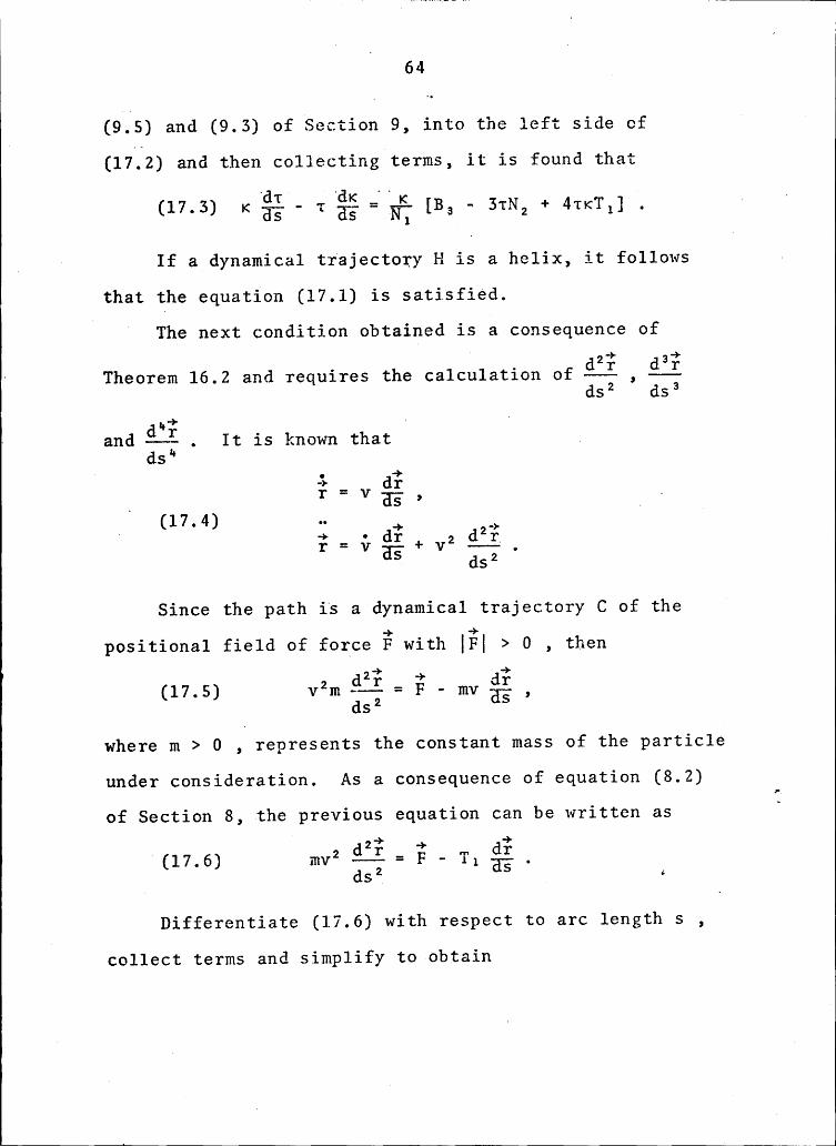
(17.2)Bysubstituting the formulas for gl and gi foundinss

a64

(9.5) and (9.3) of Section 9, into the left side of

(17.2) and then collecting terms, it is found that

(17.3) K gg - r EE =_ä% [B, — 3rN, + 4TKT1] .

· If a dynamical trajectory H is a helix, it follows ~

that the equation (17.1) is satisfied.1

The next condition obtained is a consequence of

· Theorem 16.2 and requires the calculation of-- , --dsa dsa

4* ' ’and Q-; . It is known that .

ds“

n f = v gg , U . p(17.4) „ _· + _ · a? 2 dz?I°•*VE§+V•··—·*•

dsa

Since the path is a dynamical trajectory C of the

positional field of force F with lgl > 0 , then

az? + a?(17.5) vam -- = F · mvdsa E; a

where m > 0 , represents the constant mass of the particle

under consideration. As a consequence of equation (8.2)

of Section 8, the previous equation can be written asa

az? + a?(17.6) mva -- = F — T1 .

dsa ag ‘

Differentiate (17.6) with respect to arc length s ,

collect terms and simplify to obtain

65

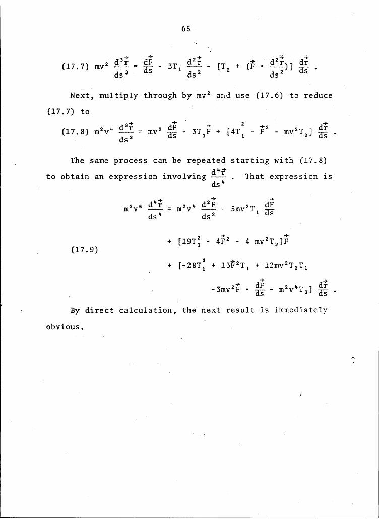
(17.7) mvz —+$ = E-- sr. ——$—- [T, + (F · ——l)] T .S dS2

_‘Next;multiply through by mvz and use (17.6) to reduceT

(17.7) to ‘ 2y

a3? _ aF ' + 2 +2 . d?(17.8) m2v“ Egg-- mvz ag - STIF + [4Tl - F · mvzlz] H; .

_ The same process can be repeated starting with (17.8)lr

to obtain an expression involving Q-? . That expression isds

msvs Q-3 = m2v“ Q-E - 5mv2T1 gg° ds“ dsz S 4

+ [19Ti — 4?2 - 4 mv2T2];_ Y (17.9) '

+ [-ZST3 + l3?2T + l2mv2T T_ 1 1 2 1_

—3mv2F • dg — m2v“T ] d?_ ' HE 3 HE °· By direct calculation, the next result is immediately

obvious.l

2

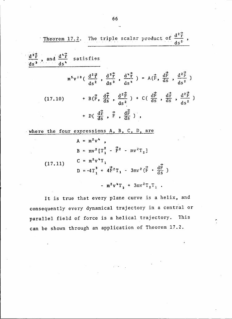
66 1.. ..62 . . 22dZ% 1

. Theorem 1722. The triple scalar product of —~; ,

...1,+i

.~é—£ , and é~£ satisfies,.....,.6

62* 62+ 6** + 6% 62%m5v’°( ——§ , -2 , -—£ ) = ACF, gg » ”*· )

ds ds° 2 ds“ dsz

— + 6¥ 62% 6% 6¥ 62%T (17-10) + BCF, gg , ggg ) + C( gg > gg > ggg )

p 6¥ + 6% 2+D(E“:F sa‘§),s

<where°the four expregsions A, B, C, D, are ·D ” A = m2v“ , = 2

i 2 2 +2 2 —. B = mv [T, — F - mv T,]

= 2 l+·(17.11) C m Z T1 + g dgD =·4T1 + 4F2T1 — 3mv2(F • ag )

It is true that every plane curve is a helix, and

consequently every dynamical trajectory in a central or

parallel field of force is a helical trajectory. This A* can be shown through an application of Theorem 17.2.

V

C (67

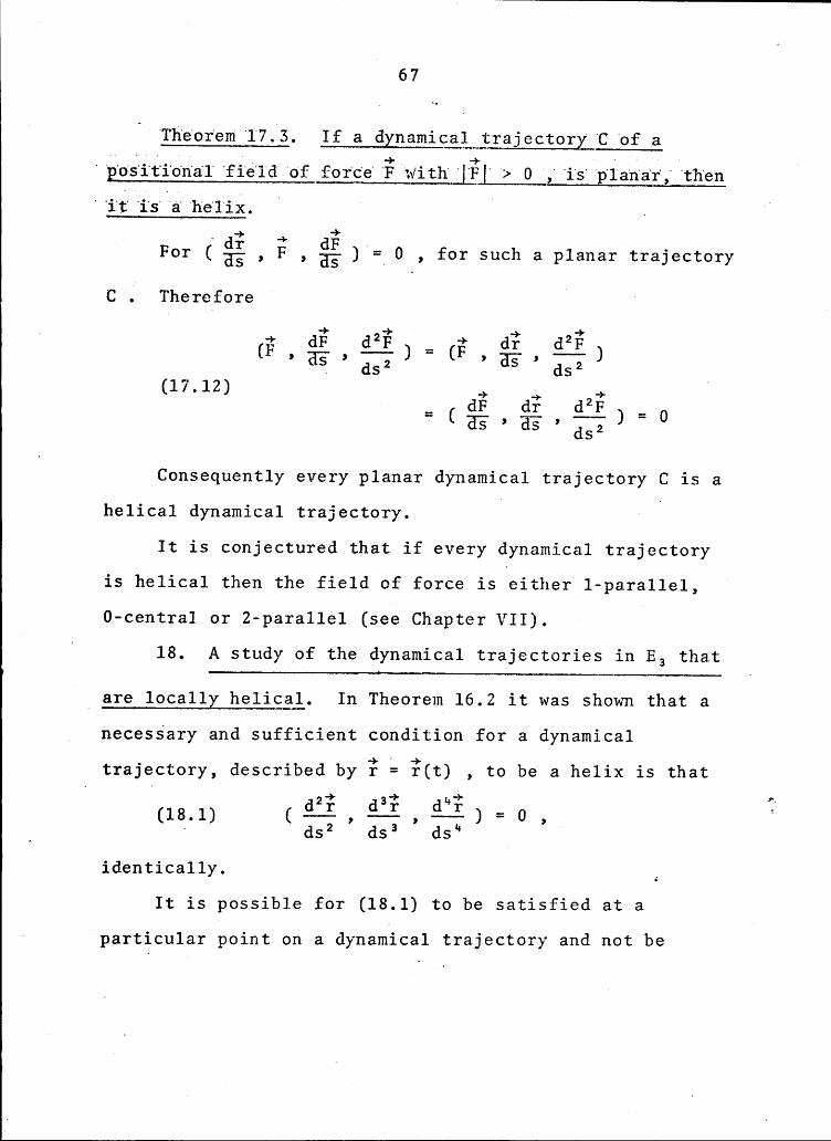
-"Theorem'17.3.' If a dynamica1mtrajectorX°C°of a0 ;·1g gianar; thena ‘·1£ is

· a? + 6% I .For ( ag , F , E; ) =AO , for such a planar tragectoryC'.Thereforeaa

„ dsa dsa(17.12) + + +

l

I dsY

‘Consequently every planar dynamical trajectory C is ahelical dynamical trajectory.

C ( I

It is conjectured that if every dynamical trajectoryis helical then the field of force is either 1-parallel, a

0-central or 2—para1lel (see Chapter VII). IU

a18. A study of the dynamical trajectories in E3 that

_ are locally helical. In Theorem 16.2 it was shown that anecessary and sufficient condition for a dynamicaltrajectory, described by r e r(t) , to be a helix is thatl

.(18.l) ( gi; , gig , gig ) = 0 , a_ ‘ dsa dsa

ds“identically. éIt is possible for (18.1) to be satisfied at a

· particular point on a dynamical trajectory and not be

satisfied at all possible points.'

This suggests the study of those points on a dynamical

trajectory for which (18.1) is satisfied.F

~

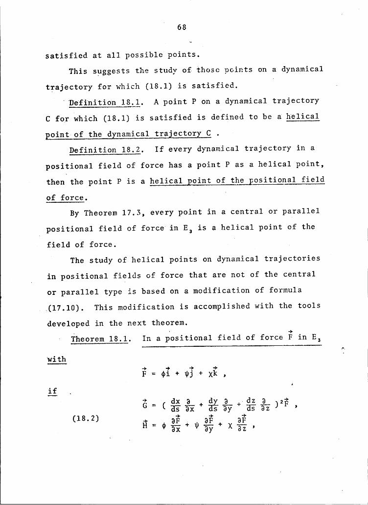
"Definition 1831. A point P on a dynamical trajectory

C for which (18.1) is satisfied is defined to be a helical

point of the dynamical trajectory C . I

Definition 18.2. If every dynamical trajectory in a

positional field of force has a point P as a helical point,

then the point P is a helical point of the_positional field

of force.t F

By Theorem 17.3, every point in a central or parallel

positional field of force in E3 is a helical point of the

I field of force. 7 F3 3

F The study of helical points on dynamical trajectories

3 · in positional fields of force that are not of the centralor parallel type is based on a modification of formula

. (17.10). This modification is accomplished with the tools

developed in the next theorem.· Theorem 18.1. In a positional field of force E in E3

Hlgl 7F = wi + wi + xF .

‘”‘”xSy oZ

‘*

69

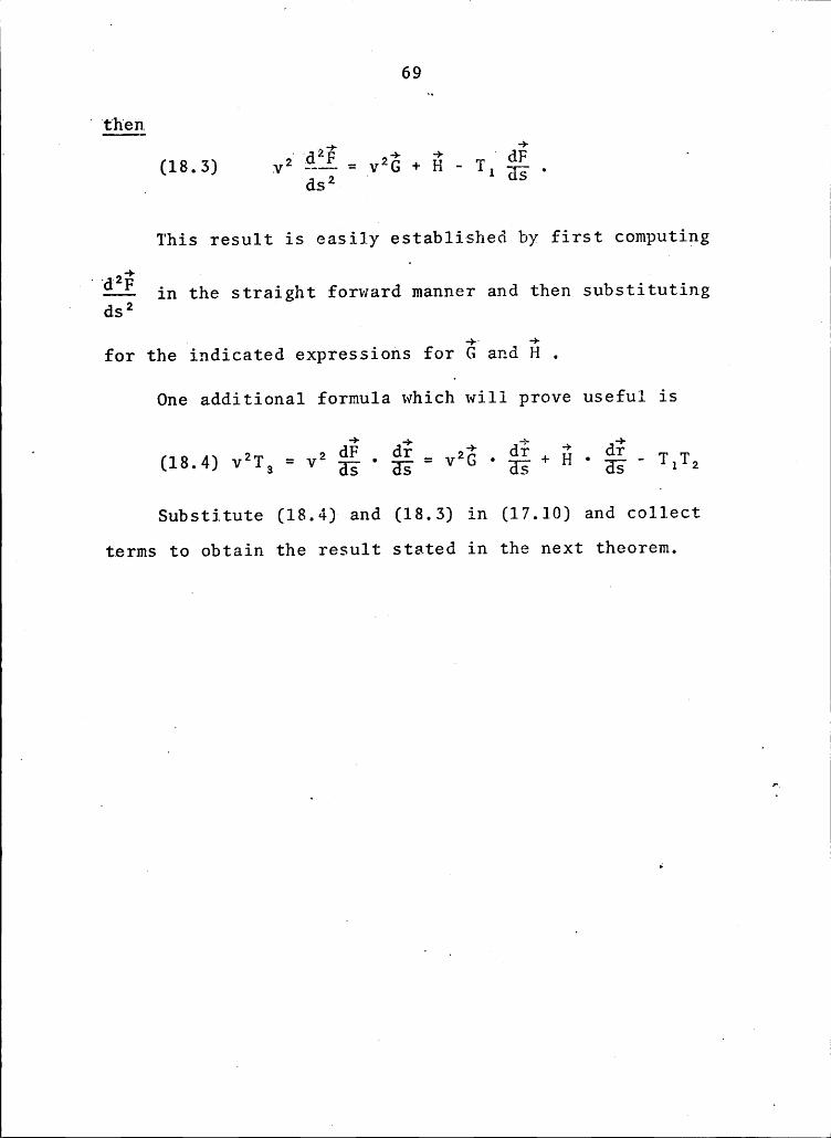
° then(

‘ 1 2· az}? ,—> ·> V ai? 1 ·(18.3) V #-~ =_V·G +-11 — T1 E-.. dsz S

This result is easily established by first computing

. . ''

1 Q-; in the straight forward manner and then substitutingds

. . I+„ +

A

for the indicated expressions for G and H .

One additional formula which will prove useful is

‘+ ·—> —> ·->' 2 = 2 dF _ dr =

2+ _ dr é _ dr _(18.4) V T3 V E; H; V G E; + H E; TITZ V

Substitute (18.4) and (18.3) in (17.10) and collect

3 terms to obtain the result stated in the next theorem.

F70„

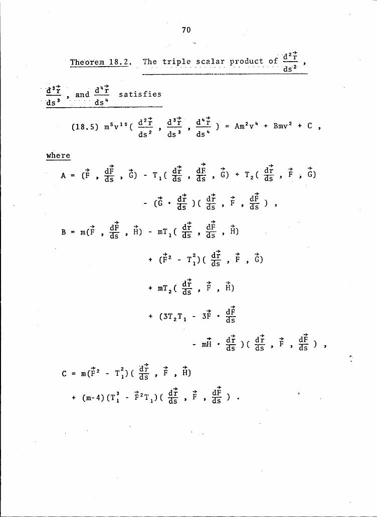
°'Theorem 18.8. The triple scalar product of Qi; , ·

Q-; , and é-ä- satisfies

( (18.5) mav1°( Q-3 , Q-1 , Q-; ) = Amava + Bmva + C ,dsa dsa ds“

where. _ + dä + d? dä + d? + +a

-A"(F2H§2G)”T1('a'§2H3f2G) +T2(H'§2F2G)

‘ + d? d? + dä· g * (G gg )( gg » F » gg ) , g+ dä + d? dä + . 1

,H) - mT1(H§,H;-, H) .

_ + (F2 ' gg , F , E)

+ .mT2( ää- . ä , H')8 F —> dä+(3T2T1 - SF • 3-;-

+ d? d? + dä" mH 2 F 2 H';) 2

g ga? + ->F

c = m(ä2 — Tf)( Hä , F , H)

+ (m-4) (T3 - ä2T )( dä Ta dä )‘

1 1

2 ·‘ l

71

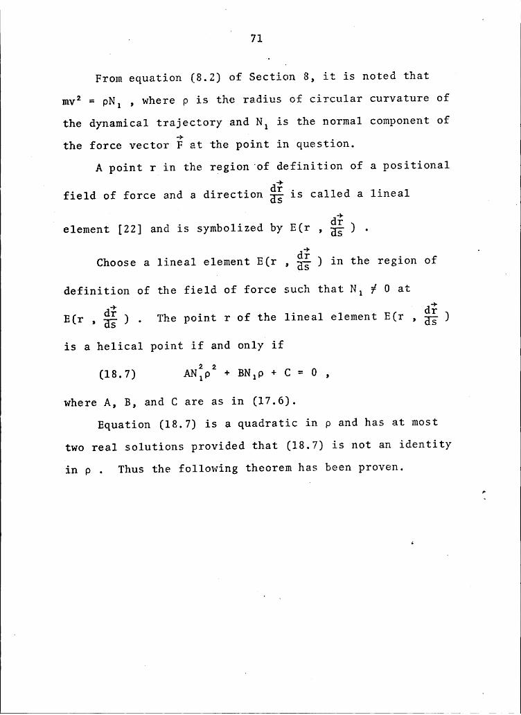
From equation (8.2) of Section 8, it is noted that ‘

mvz = pN1 , where p is the radius of circular curvature of

the dynamical trajectory and N1 is the normal component of

the force vector F at the point in question.

A point r in the region of definition of a positional—)·

field of force and a direction gg is called a linealS

S +l

element [22] and is symbolized by E(r , gg ) .+ .

Choose a lineal element E(r , ää ) in the region of

definition of the field of force such that N1 # 0 at

E(r d? ) The oint r of the lineal element E(rU d? )•.gg · P > gg

is a helical point if and only if2 2(18.7) AN1p + BN,p + C = 0 ,

where A, B, and C are as in (17.6). ‘ (

Equation (18.7) is a quadratic in p and has at most

two real solutions provided that (18.7) is not an identity

in p . Thus the following theorem has been proven.

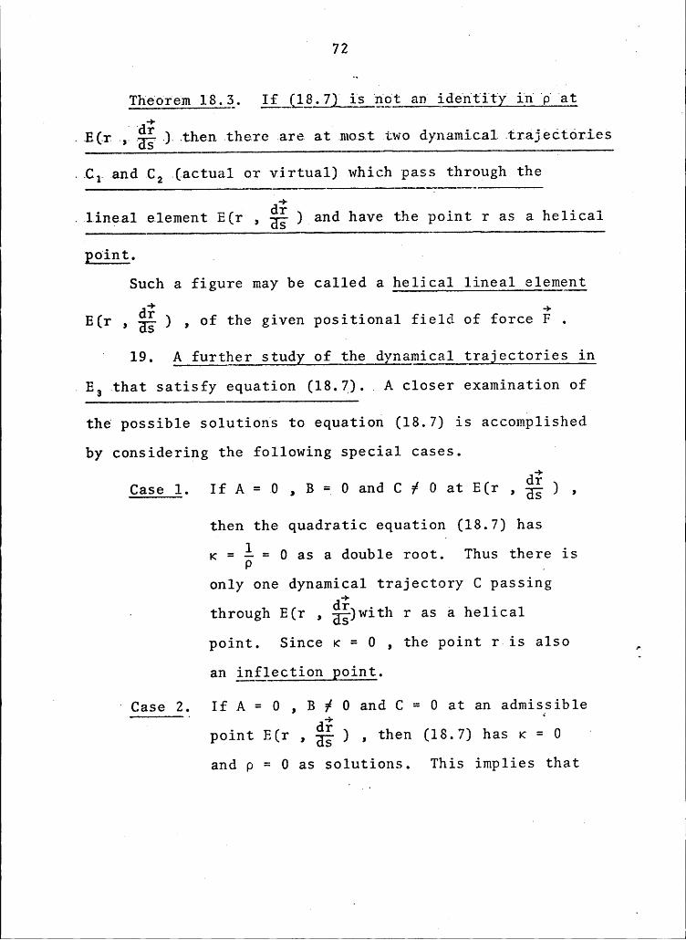
S 72A ”.

Theorem is ngt an identityin7.. +

”.E(r.,.%§ ).then there are at most two dynamical.trajectories

..CI.and.C2.(actual or virtual) which pass through the

. .1; A . ...l1D$&1 element E(r , H; )_and have the point r as a helical

vpoint. „ ~ K

Such a figure may be called a helical lineal element+

E(r , gg ) , of the given positional field of force B .‘ 19. A further study of the dynamical trajectories in

r E3.that satisfy equation (18.7).. A closer examination of

the possible solutions to equation (18.7) is accomplished

by considering the following special cases. (

_ _ 6}*Case 1. If A - 0 , B 6 0 and C # 0 at E(r , H; ) ,

then the quadratic equation (18.7) has

K = é = O as a double root. Thus there isonly one dynamical trajectory C passing

—)

- through E(r , %§)with r as a helical

point. Since K = O , the point rris also fan inflection point.

U ‘ Case 2. If A = O , B # O and C = 0 at an admissible+ Q

point E(r , ää ) , then (18.7) has K = 0 ‘

and p = 0 as solutions. This implies that

’ |

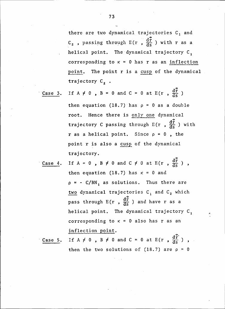
' 737

there are two dynamical trajectories C2 and’ C2 , passing through E(r 24%% ) with r as a _

_ helical point. The dynamical trajectory C13 corresponding to K =20 has r as an inflection

(°potot. The point r is a ooop of the dynamical

°trajectory C2 .

"Case 3. If A # 0 , B = O and C = O at E(r , S; )

I then equation (18.7) has p = 0 as a double

- root. Hence there is ootw_ooo dynamicaltrajectory C passing through E(r , gg ) withr as a helical point. Since p = 0 , the

point r is also a ooop of the dynamicaltrajectory.

°°Case 4. If A = 0 , B # 0 and C # O at E(r , gg ) ,

then equation (18.7) has K = 0 andS p = - C/BN1 as solutions. Thus there are

two dynamical trajectories C1 and C2 whichpass through E(r , gg ) and have r as a

helical point. The dynamical trajectory C1 2corresponding to K = O also has r as an

_

inflection point.” ‘ Case 5. If A % 0 , B # 0 and C = 0 at E(r ,

%§‘)2 .

then the two solutions of (18.7) are p = 0

2n

744

and p = Q B/AN, . This implies that there

are°£wg dynamical trajectories C1 and C2 which' pass through E(r

,4ä;) and have r as a helical

. point. The dynamical trajectory correspondingto p = 0 also has r as a cusp.

2 ‘Caset6. If A # O , B = 0 and C f 0 at E(r , gg ) ,i

then (18.7) reduces to4

(19.1) ANip2 + C = 0 .4

Equation (19.1) either has no solutions or the

solutions are p = i(- C/ANi)‘/2 . Thus, there

are gg dynamical trajectories passing through

2 E(r , gg ) with r as a helical point gr there4

are twg such dynamical traject0ries.4 If there

hare two such dynamical trajectories, then oneis an actual dynamical traiectory and theother is a virtual dynamical trajectory.

‘Case 7. If A # 0 , B f O and C % 0 at E(r , gg ) ,

then the quadratic equation (18.7) haseither no real roots, one double root or ,utwo distinct roots. Thus the number of

U_

dynamical trajectories (actual or virtual) IIthat pass through E(r , gg ) and have r '

ey

·i

75

as a helical point is either 0, 1 or 2 .In any case the point r is neither an

inflection point nor a cusp of the .

admissible dynamical trajectories.

CHAPTBR VI

..HALPHBNVS.THEOREM.IN A.EUCLIDEAN SPACE E4

20...C0nditions.for.a„curve.in.Ew.to.be.contained.in

°’a°k#f1at, with°k‘j;2’or 3. Halphen's Theorem in Bk involvesthe determination of those force fields that generate

k—flat dynamical trajectories, with k = 2 or 3. As a

result, necessary and sufficient conditions that a curve C

_ in Eu be contained in some k—flat, with k = 2 or 3, must

y be developed.Consider a curve C in Eu of at least class 3 that is

described by = r(t). Suppose this curve is not a straight

line and is contained in some 2-flat. Then there exists

fixed unit vectors A and B , and scalar constants C1 and C2 ,such that

A"

·2 $(1;) · A = cl _(20.1) + +r(t) ¥ B = C2 ·

++whereA and B are not parallel.

ADifferentiate those equations in (20.1) with respect

‘ to time, three times to obtain T

j_+. Q-; • X = 0

2 dtl ‘° (20.2) (

i+ _·56;....,; • Ä)

= 0 , .dtl 2

76

' ._ „_I

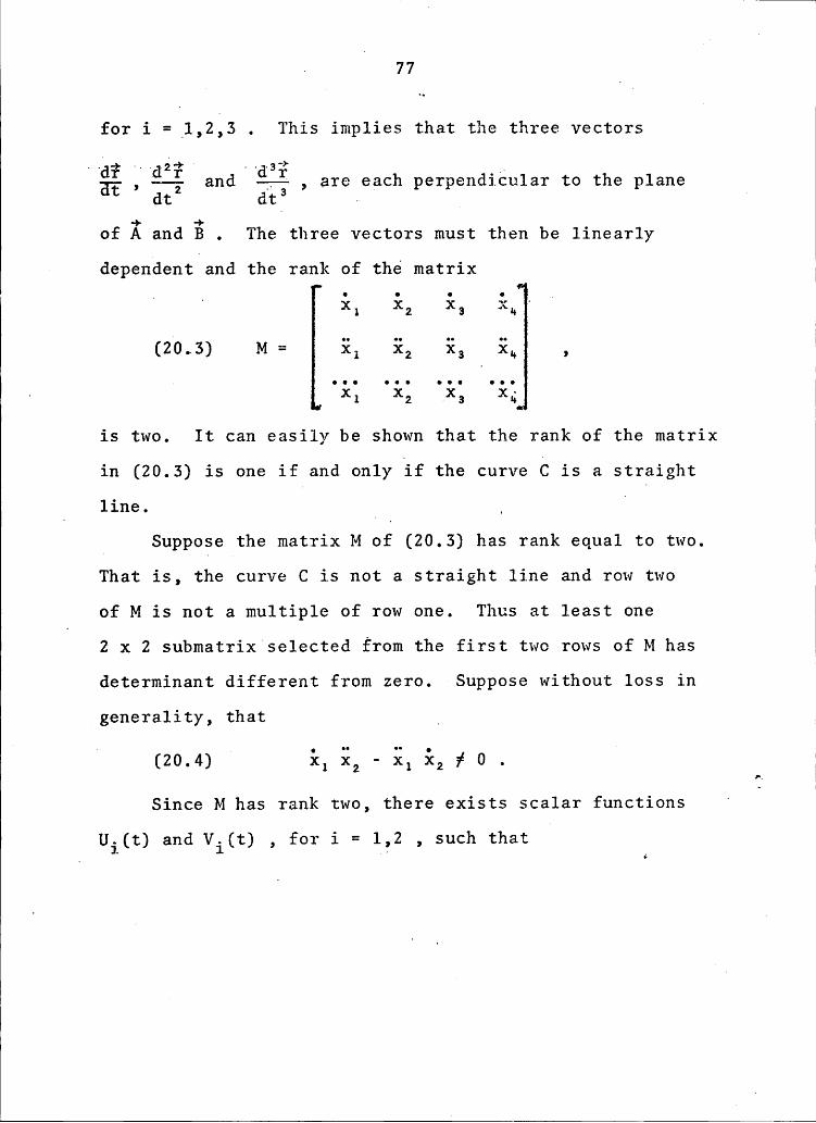
T 77

for i =_1,2,3 . This implies that the three vectors... —. . ‘ ...3** l_ lS; , Q-; and Q-3 , are each perpendicular to the plane

dt dts I. l ‘—+ +

I

of A and B . The three vectors must then be linearly~ dependent and the rank of the matrix

T ‘ xl xl xl xl · '

(20.6) M = il äl il il ,. T xlxlistwo. It can easily be shown that the rank of the matrix

in (20.3) is one if and only if the curve C is a straight

line. l _ U

Suppose the matrix M of (20.3) has rank equal to two.

That is, the curve C is not a straight line and row two

of M is not a multiple of row one. Thus at least one

2 x 2 submatrix selected from the first two rows of M has

determinant different from zero. Suppose without loss in

generality, that l( ( (20.4) T il äl — äl il ¢ 0 .Since M has rank two, there exists scalar functions ‘

_

Uj(t) and Vi(t) , for i = 1,2 , such that

l ' T

· 78 ( _

iz = Uz(t) iz + Uz(t) iz(20.5) . xz = Uz(t)_§z + Uz(t) iz

·Ü¥z = + , 6and _ _

‘ _ Stz = vzm iz + vzu;) iz(20.6) xz = Vz(t) xz + Vz(t) xz

° 'ijz = vz(1;)°5«]+From(20.5) and (20.6) it follows that

z üz(t) iz + üzgty iz = 0(20-7) - .. - .. ·

Uz(t) X1 + Uz(t) xz = 0 °

~ andiz + Özm iz = 0

0 •• • ••

0 Vz(t) xz + Vz(t) xz = 0 0

The only solution to these two systems of equations is

the zero solution since xz xz - xz xz # 0 . Therefore, itis found that Uz(t) = Cz , Uz(t) = Cz , Vz(t) = C6 and

Vz(t) = C6 where Cz, Cz, C6 and C6 are scalar constants. ,It then follows from (20.5) and (20.6) that

xz(t) = Cz xz(t) + Cz xz(t) + C6

Cz xz(t) + C6 xz(t) + C6 ,(

where C6 and C6 are constantsa

. .i 79 9

c¤5Sequen11y, if the matrix M of (20.3) is of rank

two, then the path C described by =_¥(t) is contained in

the 2~flat defined by (20.0). Therefore, the following0

.

result has been proven. 'i

Theorem 20Ll. .A necessary and sufficient condition' that a curve C described by = ¥(t) , of a least class

..three in Eu be contained in some 2·f1at but not in anyp ' l—f1at is that the matrix M of (20.3) have—rank equal tg

_ Next, consider a curve C in E, of at least class fourthat is described by r = ¥(t). Suppose this curve is

··contained in some 3·f1at but not in any 2—f1at. Thus, the

i° „ rank of the matrix M in (20.3) is three. Since C is

contained in some 3—flat, there exist a fixed unit vectorX and a scalar constant C such that g

(20.10) TIECT.) · K = c .9

By differentiating (20.10) four times, with respect to

time it is found that) _(20.11) -93 · K = 0 ,

atl ,_for i = 1,2,3,4.

_

„ This implies that the four vectors gg , Qi; ,gig,

and. dt dt

ä%ä are linearly dependent as they are all contained in the

I

same 3-flat. Thus a necessary condition for a curve Cdefined by f =_¥(t) , to be contained in a 3—flat and not

a 2—flat is that the matrix ‘ C

(gg lg)p' .3 3 3 3‘ H? dtz _dt’ dt“

have rank equal to three. From Theorem 20.1, it is noted

that the curve C is a plane curve if and only if the rank

0f.P is twoNow suppose that the matrix P of (20.12) has rank

· equal to three. Then the rank of the matrix M of (20.3) is

three and at least one 3 x 3 submatrix of M has determinant

different from zero. Suppose without loss in generality,

that‘ g . dx, dx, dx,

ät _ dt dti dzx, dzx, d2x,

C(20.13) A = ————- ————- -———— # 0dtz dtz dts °

dax, dax, dax,r dts dts dts

If P has rank equal to three, then there exists „

scalar functions Ui(t) , for i = 1,2,3 , such that

1 djx„6”(20.14) ———? = ·Z Ui(t) ——~? , _

dt 1=1 dt‘

for j = 1,2,3,4.

1 i81 °

From (20.14) the following system of equations in

Ü, , 02 and Ü, is easily obtained:· _'

2 • ..djx§ J(20.15) .2 Ui(t) -——%-= 0 ,

1=l dtz

for j = 1,2,3.- ' r 3 31

The only solution to the system of equations in (20.15)1

is the zero solution since the determinant of the coefficient1

matrix (A of 20.13) is not zero. Therefore, it is found

that U1(t) = C1 , U3(t) = C2 and U3(t) = C3 , where_ C1 , C2 and C3 are scalar constants. From the first (j=l)

A of (20.14), it follows thatv

_

i (20.16) x3(t) = C1 xl + C2 xz + C3 x3 + C3 ,

where C3 is a constant. This equation is known to describe

a 3-flat in E3 . Therefore, the following important result

has beén proven.

Theorem 20.2. A necessary and sufficient condition

tnnt_a curve C, described by f = ?(t) , of at least class

four in E3 be contained in some 3-flat but not in any

2·f1at is that the rank of the matrix P of (20.12) be equal Ö

to three.A

3 21. Positional fields of force in E3 that_generate

3 olanar dynamical trajectotion. Consider a curve C in E,

that is described by = ¥(t).„ The curve C is contained

2~ ° 82

· in a plane and not on any straight line if and only if theFmatrix M of (20.3) has rank equal to two. The followingtheorem follows immediately from that result. ‘

_ Theerem 21.1. é_dynamical'tyaject0ry C°given_hy"?’= ¥(s)‘, with s representing arc length, in a.positional field of force F with |F| > 0 , in E, is planar

. . —-*—”_ . (1}* + di? .»1f.&Rd only 1f the rank of the matrix [H; , F , ag-1*;-is°°egual to two.

n

From Theorem 21.1 it is noted that every dynamicaltrajectory of a positional field of force F with |F| > 0 ,is planar if and only if the rank of the matrix ”

, F , is less than or equal to two at everypoint on each dynamical trajectory.

Theorem 21.2. Every dynamical trajectory C of apositional field of force F with [Fl > 0 , in E, is planar

if and only if the field of force is either parallel orcentral.

The force vector acting at any admissible point is f8

(21.1) F = (F,,F2,F,,F„) ,_

where the cartesian components Fi , are functions oful

position only and are such that _21 F12 # 0 . .1:

x« i

83

Suppose a dynamical trajectory C in such a force2

field can be defined by the explicit equations

(21.2) xl =lxl (xl) , 6 ·

for i = 1,2,3. Then it is a plane curve if and only if· 1 x; · x; s

(21.3) Al = 0 x;' x;' = 0 ,

.x

0 XE' XS'and

1 ·x; xx(21.4) Al = 0 xg xx = 0 , A 2

0wherethe primes in (21.3) and (21.4) indicate derivatives

with respect to xl . This condition follows immediately

·from Theorem 20.1.i

The determinants in (21.3) and (21.4) after expanding

and simplifying are found to be equivalent toxx xx'- xx°xx = 0 ,(21.5) „xx xx'- xx'xx =

0Thefirst of equations (2.3) indicates that A l

xx = K3 xx ,(21.6) ll H1 xx = Kl xl . ·

‘ . 84-

Substitute the equations in (21.6) and their derivatives

in (21.5) to {ind that

$«Q1<;=0,.) er(21.7)

I. r

X; K: = 0 . __ _

If rg = 0 , then.x; = 0 and xt = 0 , which impliesthat the curve under consideration is contained on somestraight line. Thus every dynamical trajectory in a

4

positional field of force F with |F| > O is planar if and

only if(21.8),Ki=0,for

i = 3,4 , where the Ki are described in equations (2.3).

. Since [FI > 0 , there is no loss in generality in

assuming that F3 # O . Under this supposition the slope‘ functions ai, i = 1,2,3 , of this positional field of force

_ are defined byF2 = a1 F1 • U

(21.9) F3 = az F1 ,

F3 = a3

The Ki of equations (2.3) can then be described in

terms of the slope functions as

‘ 85

(21.10) W' A G1 ” A2where ol - w; f 0 and i = 3,4.

Ig

The equations in (21.10) can be differentiated and

W substituted in (21.8) to obtain the following twoI A

simultaneous equations.4 4

' '«

. ° 21.11 E Z A.. .·.=O( )W j=l 1=1 IJ XI XJ ’ I

1* '+b I I21.12 Z E .. . . = O °( ) ;i=1 1=1 IJ XI XJ I ” .

where30,2 Soul °^;1=¤¤,-———- @2--,Gx, Gx,

n BazA22 “ ’ ””"’•

öxzBel

A33 = QX3 ’

W A„„ = 0 ,

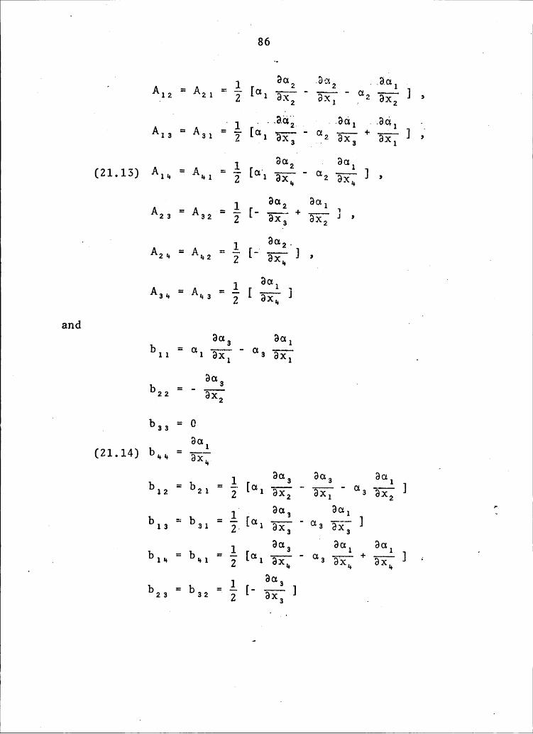
Ga .Ga ..Ga .„ 1A12 = A21 = E [G1 G2 Sg; 1 2 ‘1 ° .Q___ 1 2-« 1 A1 _’ A13 " A31 ' j [Q1‘gg; ' gz ggg +·gg: ] >

Q1 Gal(Z1•l3) A11. = A11:5Ga Ga_ _ 1 2 1

_ A22”A22”§['S}1;+g3‘l’;}»

. · GaQ _ _ 1 _ 2-A21 “ A12 ” S}: ] » .Ga A_ _ 1 1 „

and °Gas Gal

bll = ul Gxl Gxl .Gas _

b?2

b22 = 0Gal

(2]..14) bwl = gg: .Ga Ga Ga Q

_ _ 1 3 3 1b12 ' b21 ”

E[G1 S}2 ' S}?

” G2 S}; ]· G01 Ga Ü-. - 1 1 2 ____{~ b13 ” b21 " §.[G1'S};“”G3 Gxa ]

Ga A Ga Ga· _ _ 1 2 1 1 .. b1u " b¤1 ”

E [G1 S}: ° G2 S}: + S}: ] *QGa_ _ 1 2 .b23 ” b32

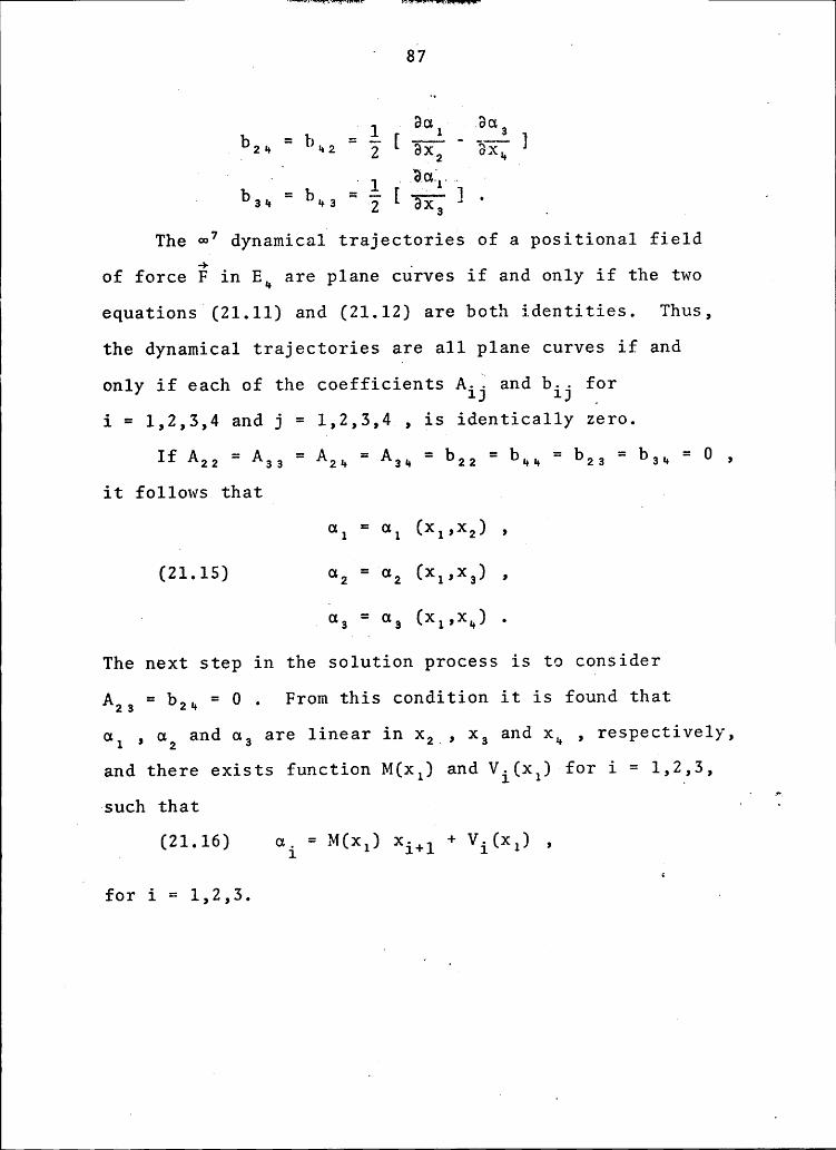
2[.;;2ej 3 · 2The wé dynamical trajectories of a positional field

of force F in E3 are plane curves if and only if the two

equations (21.11) and (21.12) are both identities. Thus,

ithe dynamical trajectories are all plane curves if and

only if each of the coefficients A15 and bij fori = 1,2,3,4 and j = 1,2,3,4 , is identically zero.

If A22 = A33 = A23 = A33 = b22 = b33 = b23 = b,„ = 0 ,

it follows that _ 2al = al (x3,x2) ,

(21.15) oz = o2 (x3,x3) ,

· 2 o3 = o3 (x1,x3) .

The next step in the solution process is to consider

A23 = b2„ = 0 . From this condition it is found that

al , az and o3 are linear in x2_, x3 and x3 , respectively,and there exists function M(x2) and Vi(x1) for i = 1,2,3,

-such that —· Ti

3 (21.16) ai = M(x1) xi+2 + Vi(x1) ,

Ifor i = 1,2,3.

‘-

1

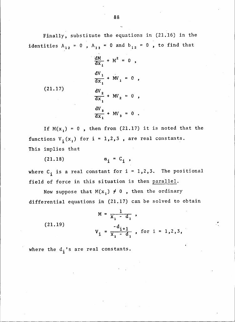
1Ü

88I

l Finally, substitute the equations in (21116) in the

identities A12 = 0 ,A12 =·0 and b12 = O , to find that

a—i-:2+ M2 = 0 9dV1 . 2HSE: + MV1 = G *

(21.17) av 2. Hi: + MV2 = 0 >I

dva ·2 H-); + MVS = Ü •

If M(x1) = O , then from (21.17) it is noted that the

functions Vi(x1) for i = 1,2,3 , are real constants.

· This implies that ‘

(21.18) ai = Ci ,

where Ci is a real constant for i = 1,2,3. The positional

field of force in this situation is then Barallel.Now suppose that M(x1) # 0 , then the ordinary

differential equations in (21.17) can be solved to obtain

M = -— 1 U><F°’ö'{’(21.19) _d_ 3

i _= , i = l,2,3,'

Iwhere the di's are real constants.

‘_

I

_ ‘ I.

( °” · II

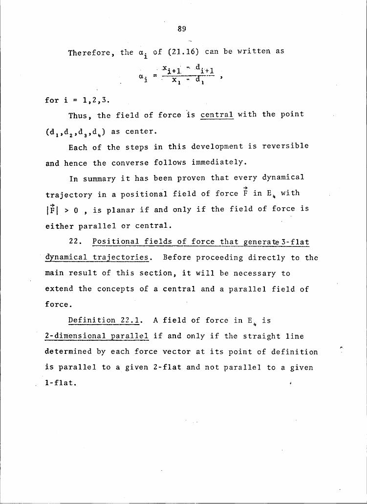
i-89

Therefore, the ai of (21.16) can be written as

Q.*1 ° -‘°‘>?;°°*’”dT ’ _for i = 1,2,3. _ y

Thus, the field of force is central with the point

(d1,d2,d3,d“) as center.Each of the steps in this development is reversible

and hence the converse follows immediately.

In summary it has been proven that every dynamical

trajectory in a positional field of force E in Eu with|§| > 0 , is planar if and only if the field of force is

either parallel or central. i

22. Positional fields of force that generate3—flat°‘dynamical trajectoriee. Before proceeding directly to the

main result of this section, it will be necessary toUextend the concepts of a central and a parallel field of

_

force. D °

Definition 22.1. A field of force in Eu isl Z—dimensional parallel if and only if the straight line

determined by each force vector at its point of definition T

is parallel to a given 2·flat and not parallel to a given.'1—flat. 1

·

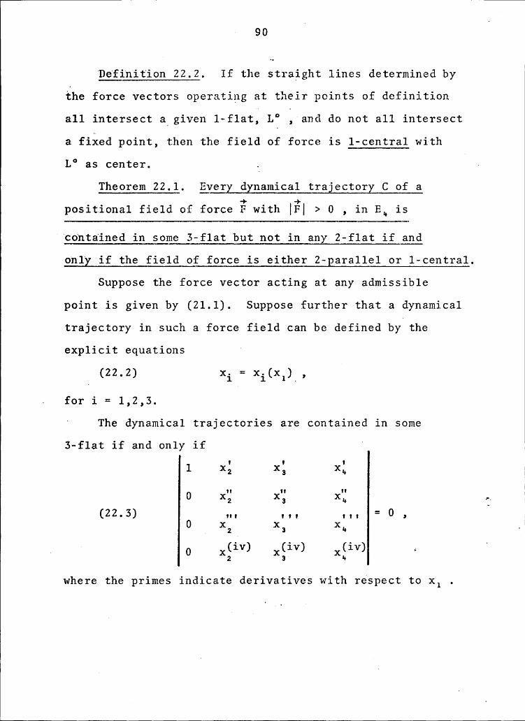
90"DefinitionZgyg. If the straight lines determined bythe force vectors operating at their points of definitionall intersect a_given 1—f1at, L° , and do not all intersect

a fixed point, then the field of ferce is l—centra1 withL° as center. l

[—

Theorem 22.1. Qyery dynamical trajectory C of a

.positional field of force g with [gl > 0 , in El is

’contained in some 3—f1at but not in any 2-flat if_andonly if the field of force is either 2—paral1e1 or l—central.

Suppose the force vector acting at any admissiblepoint is given by (21.1). Suppose further that a dynamicaltrajectory in such a force field can be defined by theexplicit equations ‘

(22.2) xi = xi(xl) ,

. for i = 1,2,3.‘ The dynamical trajectories are contained in some

3—flat if and only if '

1 x; x; x;

0 xx xg xx T ·(22.3) 0 X„, X,,, xl,. = 0 ,

z a u ·I u

Owherethe primes indicate derivatives with respect to xl .

N [

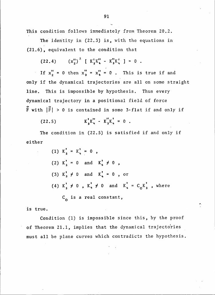
This condition follows immediately from Theorem 20.2.

The identity in (22.3) is, with the equations in(21.6), equivalent to the condition that .

(22.4) 0 . o( If xx = 0 then xg = xu = 0 . This is true if and

only if the dynamical trajectories are all on some straightline. This is impossible by hypothesis. Thus every

dynamical trajectory in a positional field of force§ with lhl > O is contained in some 3-flat if and only if

g yq IV V4

(22.5) K;K; — K;K; = 0 . (1

The condition in (22.5) is satisfied if and only if

eitherV V· (1) K; — K; j 0 ,

(2) K; = 0 and K; ¢ 0 ,C

(3) K; # 0 and K; = 0 , or

(4) K; # 0 , K; # 0 and K; = COK; , whereCO is a real constant,

is true. « n J

Condition (1) is impossible since this, by the proof° of Theorem 21.1, implies that the dynamical trajectories ;

i

must all be plane curves which contradicts the hypothesis.

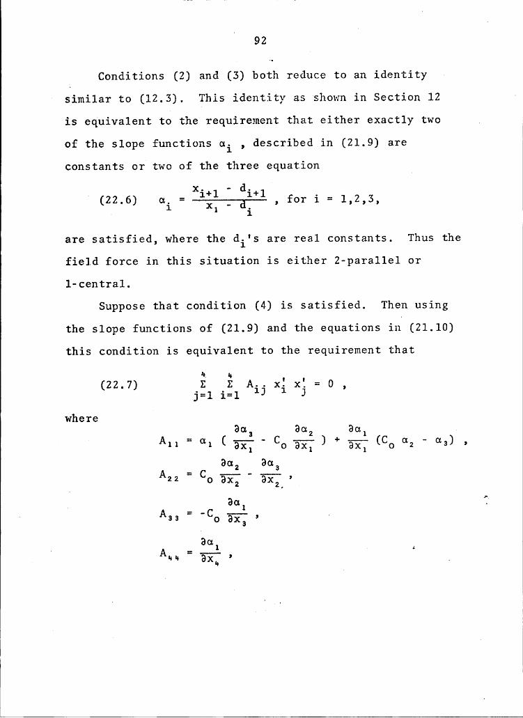
I92

Conditions (2) and (3) both reduce to an identity «

similar to (12.3). This identity as shown in Section 12 ·

is equivalent to the requirement that either exactly two 7

of the slope functions oi , described in (21.9) are

constants or two of the three equation Vx. — d. 1

i (22.6) o, = —lil———aiil , for i = 1,2,3,1 X1 · .7 1

are satisfied, where the di's are real constants. Thus the

field force in this situation is either 2-parallel or

l—central.Suppose that condition (4) is satisfied. Then using

the slope functions of (21.9) and the equations in (21.10)

this condition is equivalent to the requirement that

(227) ip. " 0. •. x- x. =j=1 i=l IJ

1whereSo, Soz Sol

So, Sog^22’“C¤ ’a°i“',"’°'ax2 ·,( Sol Ü

Sol g _A···+='2T>E';' .

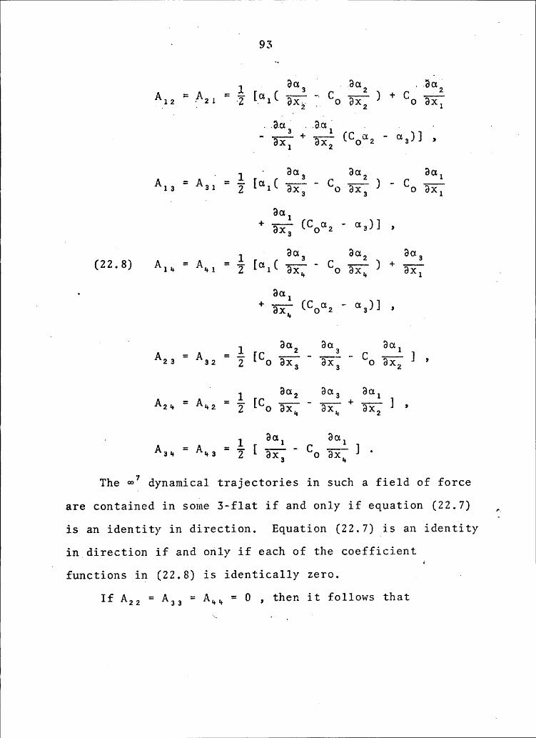
·A

935

. .65 ‘..65_= 1 „_i 2 -2 .2

Co Coöxl

..6.5; ..6.5; . . . .@3)].

r Ba Bu Bu2 2 2. 2 - 1 1A13 - A31 2 [ü1( Co gi; ) - Co Ü}?

Ga;+

'äi'; (couz ° cx·3)] a

· Ba Ba Bo_ _ 1 2 2 2

· Ba;1 + -——-32; (CO@3 · @3)] „

l 1 ' Ba Bu Sa2 2 2 ..2 - 1 - 1A23 A32 Z [Co ax; 'FE; Co 3x2 1 ’

. ' 86 Ba Bu_ _ 1 2 a 1^11‘^··¤'°i[C¤ä§j"6‘1’Ej;‘*‘ä‘«‘;1 ·. Ba Bu_ _ 1 1 1

The @1 dynamical trajectories in such a field of force

are contained in some 3—flat if and only if equation (22.7) 1is an identity in direction. Equation (22.7) is an identity

in direction if and only if each of the coefficient5

functions in (22.8) is identically zero. . ~

If A22 = A33 = A„„ = 0 , then it follows that\ .» l *

1 94

Gil

(22.9)2A

2 22 2 » H2 COo2 ~ aa =_f(x1,x3,x1) . 1

Next, suppose that A12 = A21 = 0 . This condition implies

that d1 is linear in x2 , Cdo2 - da is linear in x2 andx1 , and there exists functions M(x1) , U(x1) and V(x1)

such that ‘

a1 = M(x1)x2 + U(x1)(22.10) 2

COd2 — ag =

COConsiderthe condition resulting from M(x1) being

identically zero. For this case, A12 = A12 = 0 impliesthat U(x1) = C1 and V(x1) = C2 , where C1 and C2 arereal constants. Thus equations (22.10) reduce to

1 a1 = C1 ,2 (22.11)

CO¤2 -—d3 = C2 ;

and the force field is recognized to be 2-parallel.'Now suppose that M(x1) # 0 and consider A11 = 0 .

G12 This implies that E~E—-?—E—- is independent of x1 . j

2 O 2 3

Therefore it follows from (22.10) that' {

GU(x1) = - bo M(x1) ,

(22.12)V(x1) = - do M(x1) , .

where bo and do are real constants. With this resultT(22.10) reduces to

1 61 = _M(x1)(x2 — bo) , ·T (22.13) 'Coaz - da = M(x1)[(COx3 — x1) — do] .

( If (22.13) is substituted into the equations A12 = 0,

it is found that

(22.14) + M2 =· 0 .The ordinary differential equation in (22.14) is .

readily solved to obtain

(22.15) M = -1--L- 1 '1 X1 T Ao ,

. where AO is 8 I‘€8]. CO1'1St8I1t•The equations in (22.13) then reduce to ·

„ 1 O(22.16) _Coaz 2 ag — do 1

1 1 OThis implies that the field of force is 1-central withcenter given by x1 = Aa , x2 = bo and Coxa - x1 = do . T

lf the field of force is 2-parallel or 1—centra1, the_ latter steps can be reversed to find that (22.7) is 1

satisfied. This implies that the trajectories are

contained in some 3-flat. ·

This completes the proof of Halphen’s theorem in

Q l-

CHAPTER VII p..POSITIONAL FIELDS OF FORCE.IN En THAT.RESTRICT

' PARTICLE MOTIQQMTO (k+l)—FLAT§23.'°Positiongl°fields'of°force°that°are k#dimensional g

"paralle1. The concept introduced in this section is an1

extension of the classical parallel field of force.in

,°°Definition 23.1. A field of force in En is k-dimensional'parallel if and only if the straight line determined by

each force vector at its point of definition is parallel

to a given k-flat and k is the smallest such integer.U Definition 23.2. The direction pk of such a fixed

k-flat is defined to be the parallel dirgppipp of the 4 c

k-parallel field of force. ·U

1It can be assumed without loss in generality that the

· parallel direction of a given k-dimensional parallel field

of force is defined by

. Xj_=0»for i = k+l, k+2, ..., n .

Under this assumption, the force vector has the form

F = (F1,F2,...,Fk ; 0,0,...,0) .

_ The wzu-1 dynamical trajectories in this situation are Ü

represented by the following system of ordinary differential

. equations:

n98 ·

— __ ‘S Fi fw1=g1,2,...gk(23.1)

mxi =_‘ . ~— T ·

S where m is the constant mass of the particle.

"Theorem 23.1. In En , each dynamical trajectory of.

( a°k+dimensional parallel positional field of force with

direction pk g where 1 S k S n-l , is contained in some

(k+1) dimensional flat parallel to the direction uk .

Suppose that at t = O the particle is at

xo = [(x1)O,(x2)0,...,(xn)O] , with velocity

S XG = [(xg)0,(x2)0,--;,(Xn)0] -The trajectory described by the motion of this particle

must be contained in that part of En defined by

. (23.2)U xi = (xi)O + t(xi)0 ,

for i = k+lg k+2, ..., n .Now consider the two different situations arising

from the velocity vector xo . g

Case l. Suppose xo is parallel to the direction uk .C r This is equivalent to saying_that (xi)0 = 0

for i é k+l, k+2, ..., n . This implies that

the dynamical trajectories are contained in

-4

99C

that part of En described by

(23-3) xi = .(=<i)Ü , ”

for i = k+l, k+2, ..., n .These equations define a k—flat with

direction uk which is contained in a (k+l)

flat parallel to the direction uk .

··Case 2. Suppose xo is not parallel to the direction uk.

Then xo can be expressed in terms of its

components in the ny direction and a directionperpendicular to uk . By a rotation of theaxes holding xi fixed for l i i i k thisperpendicular direction can be made tocoinside with that of the xk+l axis.

Under this assumption it is found thatthe dynamical trajectories are contained inthat part of En described by

(23.4) xi = (xi)0 ,

for i = k+2, k+3, ..., n , which defines a j(k+l) flat parallel to uk . _

_ Thus Case l and Case 2 both lead to the described -conclusion.

l100 .

U

124.. An’additional preperty°of motien in a

'°k#dimensi0na1‘paralleI p0SitiOnal;field°of'force. Theresults obtained in this section do not relate directly to ”

Halphen's theorem. They were developed and are presented l

here to emphasize the validity of Definition 23.1.L Definition 24.1. Let P2 and P2 be two distinct

I

points in En and through P1 and P2 construct k—f1atseach with direction uk . The minimum distance between

these two k—flats is defined to be the distance from

P1 to P2 relative to the direction uk . '

In the following theorem it will be supposed that

P2 and P2 do not lie on a straight line parallel to thefixed direction uk .

Theorem 24.1. In a k-dimensional parallel_field_offorce in En , the time required by a particle in going

lfrom P1 to P2 along a fixed dynamical trajectory is

— proportional to the distance from P1 to P2 relative to_ the direction of the force field.

——————

·By the previous theorem, every dynamical trajectory 2

in such a field of force is contained in a (k+l) flatv

2 parallel to the direction uk of the field of force.1

‘Impose a rectangular coordinate system on each of .

these (k+l) flats such that a point is represented by

101

(244) (iur) = .C><„>',„y2„-··,>'k) ,

where the k—flat_defined by x =_0 is parallel to the

direction uk . The force vector in such a (k+l) flat can

be ekpressed as U(24.2) F = (0,F2,F3,...,Fk+l) ,

where Fi is a function of (x,y). The dynamical trajectories

Uof a particle of mass m in such a (k+l) flat are described

by f

ä = 0( (24.3) · „myi = Fi+l *for i = 1,2,...,k .

Suppose that at t = O the particle is at

[(X)0,(y,)0,(y2)0,---,(yk)O] with v@1¤¤itv

Under these conditions, it is readily seen that theU x-component of a point on the dynamical trajectory is given

by T(24.4) x = (i)0t + (x)0 .

1 The distance between points P1 and P2 in the (k+l)

flat relative to the direction uk is, by definition, the

difference between the x—components of the two points.

I

102

The desired result follows immediately from equation (24.4).

25. °A'eharacterizati0n ef kédimengignaligarallel

°°fie1ds'ef°ferce. A conve§se_of Theorem 24.1 is established

in the next theorem. 1 A‘ Theorem 25.1. Qpnsider·a positional field of force

..in EH.such that ·

(a) each dynamical trajectory is contained in

some (k+1)-flat, and ·(b) each such (k+l)-flat is Earallel to the

V

Q k-flats with a fixed direction uk .

If the time required in moving on a fixed dynamical

trajectory from a point P to a·Qoint Q is directly

Qrogortional to the distance from P to Q relative to the

_ fixed direction uk , then the field of force is

_ k-Rarallel. QSuppose without loss in generality that the fixed

k-dimensional direction uk , is that of the k-flat defined

bv(25.1) xi = 0 , Q

for·k+l, k+2,..., n . _ _

. Thus by hypothesis each dynamical trajectory can be

described by an equation of the form ‘

(25.2) f = (x1,x2,..t,xk;_y) ,·

103

where y is the component in a direction perpendicular to °

•U

' The time required in moving on such a dynamicalAtrajectory from a point P to a point Q is directlyproportional to the distance from P to Q relative to pk .

This implies that _

A y = constant , and(25.3) ; = O • a

This is equivalent to the condition that the forcevector at each point in such a force field has a zerocomponent in every direction perpendicular to uk . That is,

the force field is k—para1lel.A

„ 26. Positional fields of forca_rhat are (k+l)”almansional central. _Consider a positional field of forcein En in which there exists at least k force vectors which

‘ are linearly independent where 1 i k i n-1 . ‘A

Definition 26.1. If the straight lines determined by

the force vectors operating at their points of definition

always intersect a given (k-1)-flat, L£_1 , and k is the

smallest such integer, then the force field is defined to 5

be (k-l)-central with center L£_l . ·A

A _This concept is an extension of the central field of.

force that is discussed in most classical analytical

2 _ ' 104 ~l

dynamics texts. (See {12} for example.) 6

Without loss in_genera1ity, it can be assumed that the

central flat L£_1 is that described by ·

(26.1) ’ xi = 0 ,for i = k, k+l,..., n ..

U_

A force vector in such a situation has the form _

' (26.2) Ü = (F1,F2,...,Fk_l ; xkf(x), xk+lf(x),...,xnf(x))0,

where f(x) is a scalar function that is not identically zero

in the region of definition.Theorem 26.1. In a (k—l) dimensional central y

positional field of force in En with the (k—l) flat L£_l2

as center, each dynamical trajectory is contained in a

(k+l) dimensional flat passing through the center L£_l .

The dynamical trajectories under these conditions and

the assumption of constant mass m are described by

mxi = Fi for i = 1,2,...,k-l

(26.3) u .mxi = xif(x) for i = k,k+l,...,n .

In discussing these equations further, an extension of the—

method of Appell which was discussed in Chapter II is”

employed.e i

.To the system (26.3) apply the transformation

1105

°'$i1..

.yi =_E£ 1 for 1 j_1 j n but 1 f k1

(Z6-4) _ ( 16

yk = >

together with the change in time dt, = ig§~ .k k_

Note that if the (n-l) flat defined by xk = 0 is not

considered, this transformation is a one to onecorrespondence of the set of remaining points into itself.

‘ 1For the remaining discussion it will supposed that En has

been extended to a projective space, Sn , by the

introduction of an (n—l) flat at infinity. The transformation

is then a one to one transformation of Su into itself. _

1 In what follows the dots over the y's will represent

differentiation with respect to t,while dots over the x's

1 will represent differentiation with respect to the old

time t . It is shown in Chapter II that under this 11transformation, the differential equations describing the 1set of dynamical trajectories are of the form 1

(26.5) m§i = Yi { 11 1for i = l,2,...,n , where Yi is a function of yl,y2t...,yn . 11

Differentiate equations (26.4) twice with respect to· 1

time tl to obtain 1

106

for 1 i i i n, i ä k26.6 ” " ” “ ‘( )· yk ‘.“ Xkxkxk ·

Thus, the dynamical trajectories are represented by

myi = xkxkxk(Fi·- xif(x)), for l i i i k—l ,

· (26.7) myk = ·xkxkxkf(x) ,

yj = 0 ,2

- for k+l j_j j_n .

These are recognized as the differential equations

representing the dynamical trajectories in a k-dimensional

parallel field of force with direction uk defined by' I

(26.8) yj = 0 ,

for k+l i j i n . ~Note that under the discussed transformation the (k-l) -

dimensional center, L£_1 , corresponds to the direction uk .In other words, every flat Lp passing through the center

would after the transformation be a flat of the same

dimension parallel to the direction uk and conversely.

Since the transformed force field is k—kimensional

”parallel,an appeal to Theorem 23.1 finds that all the' dynamical trajectories lie in a (k+l) flat parallel to _

the direction, uk . Now apply the inverse of the discussed

pS 107

S

transformation which is itself: This transformation as

observed, sends each (k+l) flat parallel to the direction

nk into a (k+1) flat passing through the center L§_1 . I

Thus the result is established.-27. An extension of Kepler's second 1aw°of’motignp

Since the extended form of Kepler's second law of motion isU

a projective result, it will be necessary to define two

additional geometrical concepts.Definition 27.1. Suppose Lq is the flat of highest

W dimension that is parallel to both Lk and Lm , where q ivk

and q i m . Suppose Lq is generated by the orthogonal set

of vectors {u1,u2,...,uq} . Extend this set to an',orthogonal basis {u1,u2,...,uq, vq+l,...,vk} for Lk and toan orthogonal basis {u1,u2,...,uq, Wq+l,...,Wm} for Lm .

1 Lk is orthogonal to Lä if and only if every Vi for S

qfl j_i i k , is orthogonal to every Wj for q+l i j i m .

Impose a rectangular coordinate system on one of the

(k+1)-flats described in Theorem 26.1 such that a point is

represented by I

(x,,x2,...,xk_1; x,y) , T

where the central flat L§_1 is given by x = 0 , y = 0 .' ”‘Definition 27.2. Consider any point P in such a _

(k+1)·f1at. Its projection PO , into a 2—f1at LZ ,

g' 108

orthogonal to L3_1 is defined to be the orthogonal..projection]relative.toQL£_i of the point P on L2 .

In what follows it will be assumed that the projection

plane L2 is the (x,y) plane. ' 4l ‘ Theorem 27.1. In a (k—l) dimensional central field of)

.force in En with the (k-1) dimensional flat L£_l as center’°the°time reguired in going on a fixed dynamical trajectory

°’from point P to point Q is proportional to the vectorial ”

. area_O PO Q0 swept out by the radius vector of the

°'orthogonal projection of the dynamical traiectory ig_theN

”(x,y) plane. Thg_Q is the projection of the central flat

. L in the (x,y) plane. _.l<;.l................................ ,8

From Theorem 26.1 it is seen that a dynamical

trajectory passing through both P and Q must be contained

in a (k+l) flat passing through the center L£_l . In a

discussing the dynamical trajectories in such a situation,

it will be convenient to use "cylindrical" coordinates, i.e.,

xi = xi , for i = 1,2,...,k-l , _ Ü

(27.1) x = p cos G , .

y = p sin G ,‘

where. p = (x2 + y2)‘/2 and G = tan-1(y/x) .

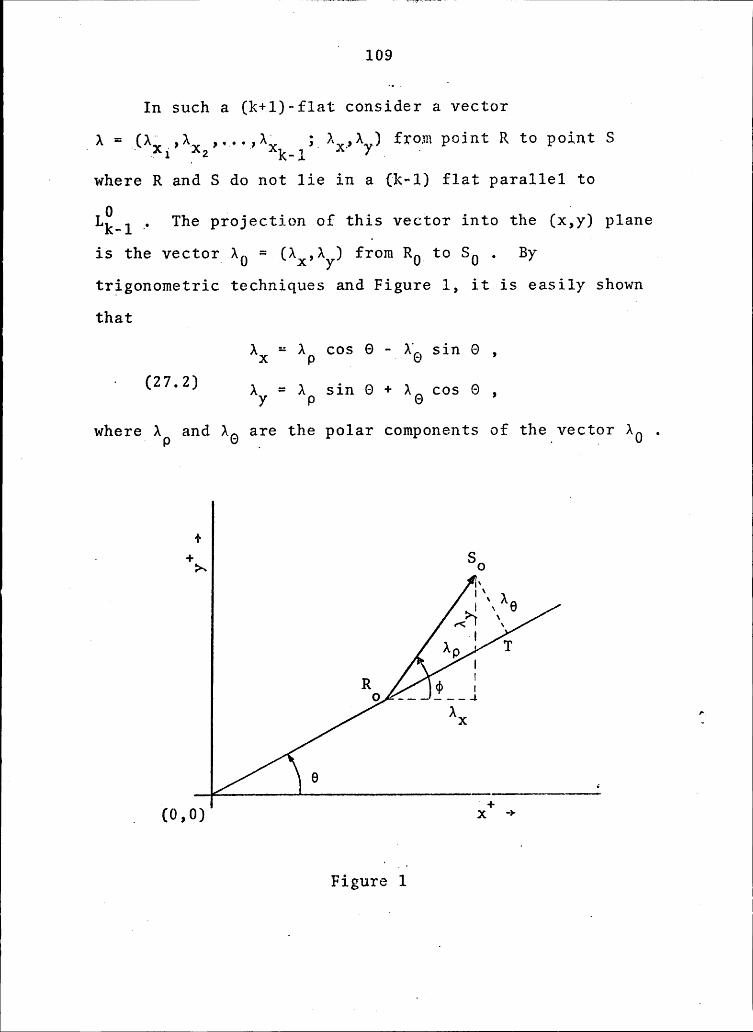
“109

In such a (k+l)-flat consider a vector B

_A =_(l#i,AX2,,,.,lXk-l;_Ax,Ay)pfrom point R to point S

* where R and S do not lie in a (k—l) flat parallel to

L£_1 , The projection of this vector into the (x,y) plane

is the vector_A0 = (lX,Ay) from RO to S0 . By ytrigonometric techniques and Figure 1, it is easily shown

thatAX= Ap cos 0 -4AG sin 0 ,

I (ZM) Ay = ip Sin 6 + A9 666 6,where Ap and AG are the polar components of the vector A0 .

+l +>— So

fx. "„ ÄI x Ü\x

II

R I6 -.. SL-;

9 6

Figure 1F

_) 110

Differentiate x =_p cos 0 and y = p sin 0 withrespecttotime t twice and it is foundthat„x

= AX =_(ö - pÖ2)cos G — (pö + 2pÖ)sin0(27.3)_ „ ( _2 · „ __ 4 —

_y = Ay =_(p - p0 )sin 0 + (p0 + 2p0)cos G .

Thus the polar components of acceleration in the (x,y)

plane are given by

A =“

- ezp P _P

(22**) AG = pe + zée .The force field is (k-1) dimensional central with

4L£_1 as center and, therefore, AG is zero.—Now pö + Zpé = 0 implies that .

T (27.4) pzé = c ,where c is a constant. This expression can be written as·

(27.5) p2dG = c dt 4

from which the conclusion of the theorem is immediate.This is an important result in that it represents an

extension of Kepler's second law of planetary motion. T

28. A characterization of (k—l) central positional

fields of force. A converse of Theorem 27.1 is established

in the following theorem. .

1 1 - lll

2 "Theorem'28.1."£f2each'dynggical°trajectory°in·a.positiona1ÜfieId.of.force2isÖB2·is~c0ntainedÄinisome°

but not.in.a k—flat2 and.thereexists..a.fixed.(k—l)

flat Lg_1 in each Lk+l such that the time

‘reguired in going on_a_fixed dynamical tralegtpry from a

°point P to a point Q is directly proportional to the_

..vectorial area, 0 PO Q0 , swept out by the orthogonal _

.projection of the motion into a plane L2 perpendicular to

.L£_l , then the force field is (k—l) dimensional central L

. with L£_1 as center. The point 0 in the plane L2 is the

.image of the fixed (k—l) flat LO .

er Consider a dynamical trajectory in such a force field

and suppose that the (kél) flat in which it is contained

has a rectangular coordinate system imposed such that the

. fixed L2 1 flat is describedby—(28.1) xi = 0 ,

2 for i = 1,2,...,k-1 . iThus, the (xk,xk+l) plane could serve as the L2 plane.

Now impose a polar coordinate system on the plane L2

by lettingxk = p cos 9 , .

L (28‘2) xk+l = p sin O , l

U Ä112

Ä area in the L2 plane is then known to satisfy

dA = Q;-d@ or(28..3)

Ä = Bi Ö

Ä

2.

This can be differentiated again and combined with (27.4)Ä

to obtain ·(28.4) Ä

=Byhypothesis t = CA where C is a constant. This

implies that Ä = 0 , which in turn implies that A9=”0

.

Since the angular acceleration about the flat L£_1

is zero, the line of action of the force vectors must pass

through the flat L£_l . Thus, the field of force is (k-l)

dimensional central with the fixed flat L£_l as center.29. An additional property of k·parallel and (k-l)

Acentral fields of force in En . The property under 2

consideration refers to the coefficient functions Kithat are defined in equations (2.3). T

Ä The force vector B acting at the point

x = (x1,x2,...,xn) is represented by (F,,F2,...,F¤) Z

The Fi are the rectangular components of the force vector

and are functions of (x1,x2,..,,xn) . Ä

113 .

The force vector is assumed to be not identically

equal to the n-dimensional zero vector. Without loss in

_genera1ity, it can be further assumed that F1 is not zero. J

Under these conditions, a set of direction functions

describing the direction of the Faraday lines of force is

_given by ° ·

‘ (29.1) 1: q,:a,:...:qn_l , ·

— where _„-i F1 °

The complete set of dynamical trajectories in Eh areJ

described by the equations of Theorem 2.1. Those equations

in terms of the direction functions di are .xy = Kixg , for i = 3,4,5,...,n

·Y( J x2' = Gxg + H(xQ)2 , y

whereBF2 v I1 v BFI

y [F2 - x;F1]G = xi §—~ - x2 E x. §—- ,I J=1 J XJ 1=1 J XJ-3

‘H = -—-——-— °

. — ür ' x;’

· a- - xt ‘„ K• = 1-1 1 ~

_ 1 al · x; '

and it is assumed that ul - x; is not zero.

114 „

i ° Theorem 29.1. If a positional field of force in En

(a)°K#parallel with k#dimensional directioni

‘°parallel’to‘that'of'some'coordinate‘(k#l)#flat,

i(b)‘(k#l)¢central with center parallel to some

l "‘coordinate‘(k#l)—flat,

..then.(n~k—l).of the (n-2) coefficient functions Ki relative

°°to’anX’dXnamical°trajectorX'have their derivatives with

. respect to xl identically equal to zero.

result is established by considering the parallel

and central cases separately.

‘°Case 1. Suppose the force field is k-parallel with

. direction uk parallel to some coordinate

Without loss in generality it

can be assumed that (n—k+l) of the n

direction functions in (29.1) are constant

p functions. In particular then it can bei

assumedthat9aj = Cj for l j_j i n-k ,

9 where the Cj are constants. ‘v Then from the expression for Ki given

in (29.2) it is noted that

i. w

115

2 (29.3) Ki =( (.C1( “ X2

where 3 j i i n-k+1 , and X; g gl X

Differentiate (29.3) with respect to

to obtain(

X 2 _ (29.4) K; =E?%;E

[-xy + Kixg] ,

for 3 j_i j_n-k+l .(

_ From the first of (29.2) it is found(

_ that the right side of (29.4) is identically .

zero. This establishes the desired result

for a k-parallel field of force.

Case 2. Suppose the force field is (k—l) central

with a coordinate (k—l) flat as center. Then

‘ (n—k+l) of the components of the force

vector F are such that

(29.5) Fi = (xi + Ci)f(xi,x2,...,xH) ,

where f(x1,x2,...,xn) is a scalar function r( and the Ci are constants.(

Without loss in generality, assume that

(29.5) is true for l i i i_n-k+l . Then by .

. definition

( · ( 116 ‘ I

. . xi +.Ci (

,(29..6) <xi_l = ,

for 2 i i i n—k+l .l '

p Differentiate the expression for Ki_given in (29.2) to obtain

' (29.7) K§ = ——l~T [a§_1 - Kia;] ,

where 3 i i i n .Next, differentiate the expression for

ai_l in (29.6) and substitute in (29.7) to

obtain 1 .

(29.8) Ki (9, C,)

where 3°i i i n—k+l . b

The right side of (29.8) seen to be

identically equal to zero by considering the

expression for Ki given in (29.2). Thus, the

' first (n—k—1) of the Ki have their derivatives

with respect to xl equal to zero. Al

This completes·the proof of Theorem 29.1.·

‘ BIBLIOGRAPHY_4

1.ET Kasner, Differential Geometric Aspects of Dynamics, _Princeton Colloquium Lectures, published by.the

· American Mathematical Society, 1913, 1934.

2.E. Kasner and J. DeCicco, Generalized DynamicalTrajectories in Space, Duke Mathematical Journal, 10(1943), pp.733—742.

3.A. Wintner, The Analytical Foundations of Celestial IMechanics, Princeton University Press (1947).

4.F. Brauer and J. Nohel, Ordinary Differential Equations,W. A. Benjamin, Inc. (1967). _

5.M. Golomb and M. Shank, Elements of Ordinary DifferentialEquations, Second Edition McGraw-Hill, (1965).

6.E. Kasner, A Notation for Infinite Manifolds, AmericanMathematical Monthly, 49 (1942), pp.243-244.

7.E. Kasner and J. DeCicco, A Generalized Theory of DynamicalTrajectories, Bulletin of the American MathematicalSociety, 48 (1942), p.833.

8.E. Kasner, The Trajectories of Dynamics, Transaction of the„ American Mathematical Society, 7 (1906), pp.401-424.

9.E. Kasner, Dynamical Trajectories: The Motion of a Particlein an Arbitrary Field of Force, Transactions of theAmerican Mathematical Society, 8 (1907), pp.l35—l58.

10.D. M. V. Sommerville, An Introduction to the Geometry of N‘ Dimensions, Dover (1958).

ll.E. Sperner and O. Schrier, Modern Algebra and Matrix Theory, ÖChelsea (1959). 2

12.E. T. Whittaker, A Treatise on the Analytical Dynamics ofParticles and Rigid Motions, Fourth Edition, DoverPublications (1944).

13.J. A. Todd, Projective and Analytical Geometry, PittmanPublishing Corporation·(l946).’ · I

II

I____i_.

‘l18 g

_ 14,E. Kasner and J. DeCicco, Geometrical Properties ofPhysical Curves in Space of N Dimensions, Revista deMatematica y Fisica Teorica de la Universidad Nacional

I delTucuman,15rD.

J. Struik, Analytic and Projective Geometry, Addison-Wesley (1953).

16.P. Appel, De L'Homographie en Mecanique, American Journalof Mathematics, 12 (1890), pp.l03—1l4.

17.E. Kasner and J. DeCicco, Generalizations of Appell's UTransformation, Journal of Mathematics and Physics,27 (1949), pp.262—269. ‘

18.G. E. Shilov, An Introduction to the Theory of LinearSpaces, Translated by R. A. Silverman, Prentice-Hall,Inc. (1961). _

19.E. T. Browne, Introduction to the Theory of Determinants”

and Matrices, University of North Carolina Press (1958).

20,E. Kasner and J. DeCicco, The Geometry of Velocity Systems,Bulletin of the American Mathematical Society, 49(1943), pp.236-245.

21.D. M. V. Sommerville, Analytical Geometry of Three· Dimensions, Cambridge University Press (1959).

22.J. DeCicco, The Riemannian Geometry of Physical Systems ofCurves, Annali Di Mathematica, Pura ed Applicata, SerieIV, Tomo LVII (1962), pp.339-403.

23.T. J. Willmore, An Introduction to Differential Geometry,Oxford University Press (1959).

24.W. Graustein, Differential Geometry, Dover (1966).

25.H. Guggenheimer, Differential Geometry, McGraw—Hill (1963),_

C 26,B O'Nei1l, Elementary Differential Geometry, AcademicPress (1966). · ,

l27.E. Kreyszig, Differential Geometry, University of Toronto I

Press (1959). ·i

‘ U119

t z3,A. Fialkow, Initial Motion in Fields of Force, pTransactions of the American Mathematical Society, 40(1936), pp.495·501.'

29.E. Kasner and D. Mittleman, Extended Theorems in Dynamics,Science, 95 (1942), pp.249-250.

~ 30.E. Kasner and D. Mittleman, A General Theorem of theInitial Curvature of Dynamical Trajectories, Proceedingsof the National Academy of Sciences, 28 (1942),pp.48-52.

31.J. DeCicco, Extensions of Certain Dynamical Theorems ofi

_ Halphen and Kasner, Bulletin of the American MathematicalSociety, 49 (1943), pp.736—744.

32.J. DeCicco, Dynamical Trajectories of the Curvature Type,Proceedings of the National Academy of Sciences, 29(1943), pp.268—270.

33.E. Kasner, Dynamical Trajectories and Curvature _Trajectories, Bulletin of the American MathematicalSociety, 40 (1934), pp.449-455.

34.J. DeCicco, Dynamical and Curature Trajectories in Space,Transactions of the American Mathematical Society, 57(1945), pp.270-286. 2

35.0. Veblen and J. Young, Projective Geometry, Volume 1,Ginn and Company (1910).

36.E. Kasner and J. DeCicco, Transformation Theory of‘ Physical Curves, Proceedings of the National Academy

of Sciences, 33 (1947), pp.338—342.

37.R; C. Buck, Advanced Calculus, Second Edition McGraw-Hill,(1965).

38.E. Kasner and A. Fialkow, Geometry of Dynamical TTrajectories at a Point of Equilibrium, Transactions ofthe American Mathematical Society, 41 (1937), pp.314-320.

39.A. Dresden, Solid Analytical Geometry and Determinants,John Wiley and Sons (1946). ·

40.E. Kasner, Differential Equations of the Type; y°°' ä

Gy°° + Hy°°2 , Proceedings of the National Academy of TSciences, 28 (1942), pp.333·338.

1

sHALPHEN'S THEOREM AND RELATED RESULTS

UGeorge Edward Culbertson

i.

Abstract .

Halphen's Theorem states that, "A necessary and

sufficient condition for every dynamical trajectory in aE

positional field of force in E3 to be planar is that

the field of force is either parallel or central." This

g result has been known for some time, however only the‘ sufficiency part of the theorem is widely documented.

E A new analytic proof of the necessity part of

Halphen's Theorem was developed. The details of this

proof motivated the new concepts of a flat point in a

field of force and a flat point on a dynamical trajectory

in a positional field of force. Several new results

related to Halphen's Theorem were then obtained. One

such result is a less restrictive version of Halphen's

Theorem which states that, "A positional field of force

„A

in E3 is either parallel or central if and only if at

each point P there exists six distinct directions, notall of which are on a quadric cone with vertex at P,

l such that each dynamical trajectory that passes through

P in one of these six directions has P as a flat point."

Those positional fields of force that generate

helical paths were studied and the new concepts of a '

helical point of a field of force and a helical pointA

o on a dynamical trajectory were defined. One of the newV results obtained states that, "If a point P is not a helical

point of a positional field of force in E3, then in eachdirection through P there passes at most two dynamical

y traiectories that have P as a helical point."

The definitions of a k—parallel field of force and aV

(k—l)-central field of force were structured with the

_goal of extending Halphen's Theorem to higher dimensional

space. A k-parallel field of force is one in which the lines

of action of the force vectors at their points of definition

are all parallel to a given k—flat and k is the smallest

such integer.VA

(k-l)—central field of force is one in

. which the lines of action of the force vectors at their

point of definition all intersects a given (k—l}—flat and

k is the smallest such integer.

4 _ An extension of Halphen's Theorem to a Euclidean space

of dimension four was obtained. That result states that,

"Every dynamical trajectory in a positional field of force

in E4 is contained in some k-flat, with k = 2 or 3, if and ' ionly if the field of force is either (k=l)—paral1e1 or Ä

(k—2)·central. E

ll

A partial extension of the theorem to Euclidean spaces

En with n>4, was developed. This result states that,

"Every dynamical trajectorv in a k-parallel or aU

p (k-l)-central field of force in En with kin—l, is contained_ in some (k+l)—flat."

Other classical dynamical results in E3 were extended

to En through the use of the new concepts of a k—parallel

and a (k-1)-central field of force.