Table of Contents

1. Introduction ......................................................................................................................................... 3

1.1 Introduction ................................................................................................................................... 3

Preservation and deformation ........................................................................................................ 3

1.2 Complementing modeling and experiment .................................................................................. 3

Properties of wood (orthotropic material)...................................................................................... 3

Experiments ..................................................................................................................................... 4

Modeling.......................................................................................................................................... 5

2. Model .................................................................................................................................................. 5

2.1 Modeling steps .............................................................................................................................. 5

2.2 Model parameters ......................................................................................................................... 6

2.3 Parameter study: Modeling parameters ....................................................................................... 6

3. Results ................................................................................................................................................. 8

3.1 Parameter study: parallelity .......................................................................................................... 8

3.2 Comparison to experiment.......................................................................................................... 10

4. Discussion .......................................................................................................................................... 12

5. Conclusions and recommendations .................................................................................................. 17

Reference .............................................................................................................................................. 18

3

1. Introduction

1.1 Introduction

The Vasa ship sank during its maiden voyage in 1628, when a gust of wind caused it to tilt

and let water in through the cannon holes. The main reason for this was that it was too top

heavy and had too little ballast giving it bad stability. For hundreds of years it lay on the sea

bottom until 1961, when it was salvaged. In 1959 they started to lift the ship, bringing it

closer to the shore where it was easier to handle. The final lift took place in 1961 when it

was raised to the surface. It was first placed in a temporary building and later moved into its

own museum in 1988 were it is located today.

Preservation and deformation

Over the years it has become apparent that the ship slowly deformed, creeping a few

millimeters every year. The major reason is probably the treatment with Polyethylene glycol,

called PEG, that is used to preserve waterlogged wood. It replaces the water and keeps the

wood from warping or shrinking when it dries. But it also results in the wood getting soft.

Other major reasons might be sulfuric acid created by oxidation of sulfur from polluted

water and iron ions or nanoparticles from the iron bolts that contributes to the aging of the

wood. The current support structure is not enough to keep the ship intact and therefore a

new support structure is needed.

In order to design an improved support structure the ship and its wood needs to be

examined. The experimental and numerical studies are done by Uppsala University at the

institution of applied mechanics.

1.2 Complementing modeling and experiment

Properties of wood (orthotropic material)

Many materials, such as metal or glass, are considered isotropic, meaning that they are

homogeneous and have the same material properties in all directions. Wood on the other

hand is an orthotropic material, meaning that it has three orthogonal axes with different

mechanical properties. The properties in these directions can be considered to be the same

everywhere in the wood. The three axes of wood are longitudinal (parallel to the trunk of

the tree), tangential (parallel to the year rings), and radial (outwards from the trunk of the

tree).

When a material is affected by a sufficiently small force it deforms elastically, meaning that it

returns to its original form when the force is removed. During elastic deformation the

relationship between stress (load force per area) and strain (relative deformation) in one

dimension is constant according to

4

where ε is the strain, σ is the force per area and E is Young’s modulus. In the study we are

only considering elastic deformation.

Since wood is an orthotropic material it has different material properties in different

directions: one Young’s modulus for the longitudinal direction, another for radial and a third

for tangential. The model will only consider a force in one of the axes and therefore only one

Young’s modulus will be necessary.

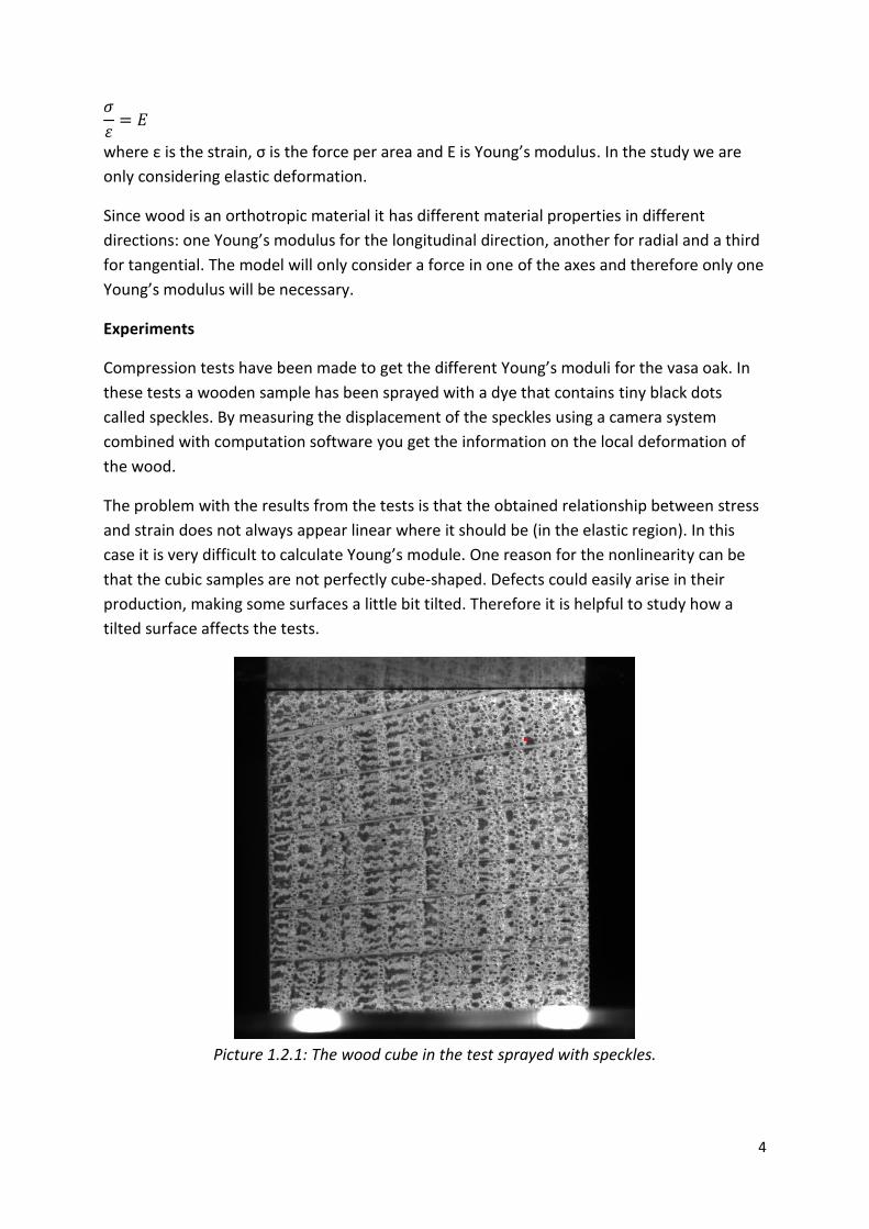
Experiments

Compression tests have been made to get the different Young’s moduli for the vasa oak. In

these tests a wooden sample has been sprayed with a dye that contains tiny black dots

called speckles. By measuring the displacement of the speckles using a camera system

combined with computation software you get the information on the local deformation of

the wood.

The problem with the results from the tests is that the obtained relationship between stress

and strain does not always appear linear where it should be (in the elastic region). In this

case it is very difficult to calculate Young’s module. One reason for the nonlinearity can be

that the cubic samples are not perfectly cube-shaped. Defects could easily arise in their

production, making some surfaces a little bit tilted. Therefore it is helpful to study how a

tilted surface affects the tests.

Picture 1.2.1: The wood cube in the test sprayed with speckles.

5

Modeling

Through the finite element method, called FEM, it is possible to simulate the compression

test using a numerical model. FEM subdivides a structure into a number of sub elements

(finite elements) and then approximates a function for each segment separately. In this case

two pieces of geometry are divided into a mesh of finite elements and the deformation and

displacement are approximated in each segment.

For the numerical modeling COMSOL has been used. COMSOL has built-in physics and

structural modeling, including FEM.

2. Model

2.1 Modeling steps

The first step in the modeling was to make a perfect cube and add a boundary load to test

the model, as well as to learn about COMSOL. Then the top side was tilted by adding a

parameter that specifies the angle of the top relative to the horizontal plane. To complete

the model a second component, a square block, was added to compress the cube. The

contact pressure was simulated by defining a contact pair between the top surface of the

cube and the bottom of the block. A prescribed displacement of the block was defined and

changed through a parametric sweep, thus simulating the block compressing the cube little

by little.

Picture 2.1.1: The cube bellow that is compressed by the block on top.

6

2.2 Model parameters

Since the dimensions of the cube shouldn’t matter they have been set to 1 (m). The

dimensions of the top block were set to 1.25 (m) on both sides of the contact base and 0.25

(m) high. It was set to be broader than the cube so that when the cube expands on the sides

it would still be compressed over the whole surface.

The boundary conditions need to be set to keep cube from moving around but at the same

time allow it to expand and compress. The cubes bottom surface is constrained in z-direction

(up and down). One of the edges of the bottom surface perpendicular to the y-direction was

constrained in that direction. Another edge of the bottom surface that was perpendicular to

the x-direction was constrained in that direction.

The top block was constrained in x and y-direction and has a prescribed displacement in the

z-direction.

Friction is ignored in this model. It is not believed that it will have any significant effect on

the results.

The type of mesh used for the major studies was a sweep of free quad. Which means the

model is divided into cubic elements. The other type of mesh used was tetrahedral that

divides the geometry in tetrahedrons.

For the material parameters of the cube Young’s module is set to GPa and Poisson’s

ratio to 0.3. The density should not affect our calculations, but COMSOL requires it before

calculating so it was set to 630 kg/m3.

For the results it should not matter what the block has for Young’s modulus, Poisson’s ratio

or density, since it is constrained in all directions, but since COMSOL demands it before

calculating they was set to 1 2300 GPa, 0.3 and 1 kg/m3.

2.3 Parameter study: Modeling parameters

The model has been tested with both isotropic and orthotropic material parameters. No

significant difference between the results was noticed when the compression was parallel to

one of the orthotropic material’s axis. A tilted material angle gave a different result, but this

is outside of the scope of this study. The tests only studies load applied in one of the

material’s axes.

The mesh refinement was studied. In the case of the cube being perfectly parallel the

different refinements gave the same results (with an error of 10-12). When testing with

contact and tilted surface the difference between meshes was somewhat noticeable (picture

2.3.1 and 2.3.2). As seen in the pictures the mesh converges. For the mesh used in the major

7

studies (that is named Course) the error is neglect able. It would not have any significant

effect to the results if a finer mesh was used, but it would take more time to calculate.

Picture 2.3.1: Graph for different mesh refinements of quad type. Where the y-axis stands for

how much the upper block has moved and x-axis is the strain of the short side (see picture

3.1.1). Blue is the most unrefined and pink the most refined.

Picture 2.3.2: Graph for different mesh refinements of tetrahedral type. Where the y-axis

stands for how much the upper block has moved and x-axis is the strain of the short side (see

picture 3.1.1). Blue is the most unrefined and pink the most refined.

Refinement

– Extra Course

– Courser

– Course

– Normal

– Fine

Refinement

– Extra Course

– Courser

– Course

– Normal

– Fine

8

3. Results

3.1 Parameter study: parallelity

Three sides of the cube were studied: the short side, tilted side and long side (Picture 3.1.1).

The stress was calculated by the surface average stress of the top surface of the cube (which

comes from the compression from the block). The strain for each surface was calculated by

the surface average strain of each respective surface.

Picture 3.1.1: A short side, B tilted side, C long side and D top surface.

The model was calculated for seven different angles of the tilt, starting with 0° and then

increasing with 0.5° until 3°. The graphs for the stress and strain are shown in Picture 3.1.2

for the short side, Picture 3.1.3 for the tilted side and 3.1.4 for the long side.

9

Picture 3.1.2: The stress strain graph for the short side of the model with different angle of

tilt. The linear blue line is a perfect cube.

The short side is elongated in the beginning hence the graph (Picture 3.1.2) shows some

positive strain that is more noticeable for larger angles. After that in the negative region of

strain the graph becomes linear. This all is making it look stiffer.

Picture 3.1.3: The stress strain graph for the tilted side of the model with different angle of

tilt.

– No angle

– 0.5°

– 1°

– 1.5°

– 2°

– 2.5°

– 3°

– No angle

– 0.5°

– 1°

– 1.5°

– 2°

– 2.5°

– 3°

10

Regardless of the angle the stress-strain relationship of the tilted side remains linear (Picture

3.1.3).

Picture 3.1.4: The stress strain graph for the long side of the model with different angle of tilt.

The linear blue line is a perfect cube.

The long side shows a smaller slope that increases until it becomes linear. The nonlinear

slope shows that it takes less force to compress the side in the beginning. (Picture 3.1.4)

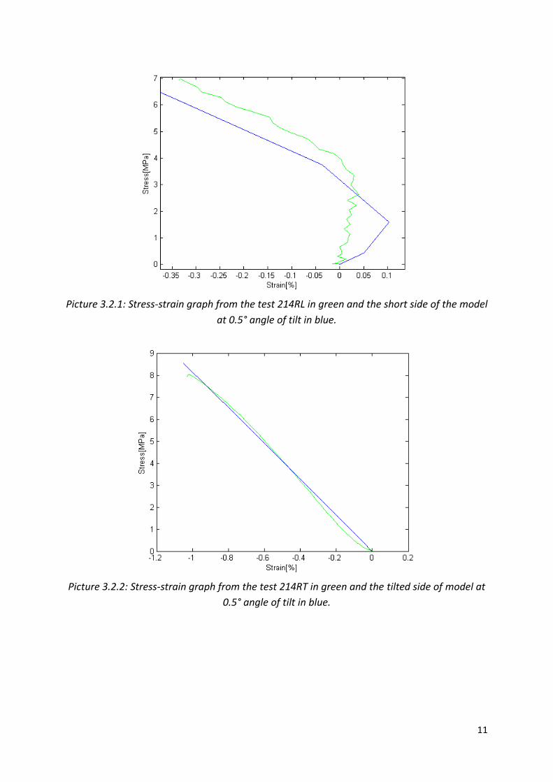
3.2 Comparison to experiment

When comparing to the real experiments I discovered a test that was similar to what was

shown in the model. It was called 214RL, where 214 is the sample number, R means

compression in the radial direction of the wood and L means that expansion in longitudinal

direction was studied. By scaling the stress from the short side at 0.5° with a factor of 20/3 a

graph similar to 214RL was obtained (Picture 3.2.1). Using the same parameters the result of

short side was compared to test 214RT (Picture 3.2.2). T means that expansion in the

transverse direction was studied, which makes it the tilted side if 214RL was the short side.

– No angle

– 0.5°

– 1°

– 1.5°

– 2°

– 2.5°

– 3°

11

Picture 3.2.1: Stress-strain graph from the test 214RL in green and the short side of the model

at 0.5° angle of tilt in blue.

Picture 3.2.2: Stress-strain graph from the test 214RT in green and the tilted side of model at

0.5° angle of tilt in blue.

12

4. Discussion

The result from the model is quite natural and is what you should expect from the non-

parallel cube. There is a smaller contact area in the beginning which results in smaller force

is needed to compress the long side. The short side is elongated due to the long side being

compressed. When the cube has been compressed so much that the whole top surface is in

contact the surface is compressed equally, thus both graphs becomes linear (see picture

3.1.2 and 3.1.4).

The stress-strain graphs of the short side and the long side showed increasing nonlinear

graphs with increasing angle of tilt, but for high enough stress all angles showed a linear

behavior. The slope of the linear part was the same for all angles (including zero); therefore I

can draw the conclusion that the Young’s modulus could be calculated from the slope of any

linear part. In tests that showed results similar to the model it should be possible to calculate

their Young’s module by the slope of the linear part.

The tilted side showed a linear graph for all angles of tilt. In the beginning the lower end,

closest to the short side, is elongated but this is compensated by the higher end, closest to

the long side, which is compressed more; thus the average becomes a linear line. The very

small difference between the lines in picture 3.1.3 might just be some error in the model

calculation.

Two tests, 214LR and 222LT showed completely nonlinear graphs (picture 4.1 and 4.2). This

may be the effect of a short side as seen in picture 3.1.2. What contributes to this is the

general shape of the stress-strain graph and that some strain values from the 214 test

indicate expansion. The linear part shown in the model graph might be outside the elastic

region of those tests.

What speaks against it is that the model clearly show tension in the beginning and then

compression, during which the graph becomes linear, the 214 test showed very little tension

and the 222 test showed almost no tension.

13

Picture 4.1: Test 214LR stress-strain graph in blue.

Picture 4.2: Test 222LT stress-strain graph in blue.

When looking at the local displacement one expects a graph with lines of color gradients

that is horizontal for the displacement parallel to the load force (picture 4.3) and vertical for

the displacement perpendicular to the load force (picture 4.4). But the 214LR and 222LT

tests did not show this behavior; instead the displacement graphs almost have lines at 45°

angle (picture 4.7, 4.8, 4.9 and 4.10). When looking at the sides of the model only the tilted

side showed a similar graph (picture 4.5 and 4.6), especially compared to test 214LR (picture

4.7 and 4.8).

14

Picture 4.3: The displacement parallel to the load force from the model for a perfect cube

Picture 4.4: The displacement perpendicular to the load force from the model for a perfect

cube

Picture 4.5: Displacement parallel to the load force for the tilted surface from the model. The

cube is compressed in the bottom and the top is stationary.

15

Picture 4.6: Displacement perpendicular to the load force for the tilted surface from the

model. The cube is compressed in the bottom and the top is stationary.

Picture 4.7: Displacement parallel to the load force for test 214LR. The cube is compressed in

the bottom and the top is stationary.

Picture 4.8: Displacement perpendicular to the load force for test 214LR. The cube is

compressed in the bottom and the top is stationary.

16

Picture 4.9: Displacement parallel to the load force for test 222LT. The cube is compressed in

the bottom and the top is stationary.

Picture 4.10: Displacement perpendicular to the load force for test 222LT. The cube is

compressed in the bottom and the top is stationary.

The stress-strain graph for the tilted side is completely linear but the graphs from 214LR and

222LT are nonlinear, which means it is probably not the effect of the tilted side. The graph

looks like the tilted side in one corner but in the opposite corner it also looks like the tilted

side with the color reversed. This could mean that it is the effect of a parallelogram formed

side (looks like a tilted side on the bottom and top with the diagonal as a symmetry line),

though it has not been studied in this project.

17

5. Conclusions and recommendations

For test results that are similar to the results from the model (Picture 3.1.2, 3.1.3 and 3.1.4)

it is possible to calculate their Young’s modulus from the slope of their linear part.

The 214RL and 222RT showed no linear part and that is probably the effect of something not

studied in this model. When comparing the local displacement with the model it indicated

that 214RL might have a parallelogram surface.

In future research I would recommend studying things that were not implemented in my

model. One such thing is the effect of a parallelogram surface. The results indicated that one

sample test (214RL) might have that form. The inhomogeneity of the wood might also affect

the results. The model was isotropic because the tests only studied load applied in one of

the wood’s orthotropic axes. One can never get the axis exactly parallel to the force though,

and it can therefore be worth to study. Another thing that was not studied but that might

affect the result is friction.

18

Reference

Almkvist, Gunnar The Chemistry of the Vasa –Iron, Acids and Degradation SLU, Uppsala 2008