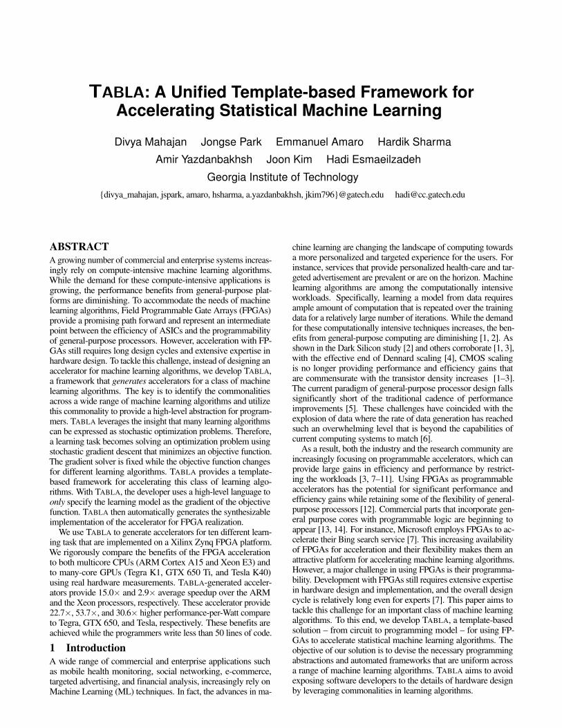
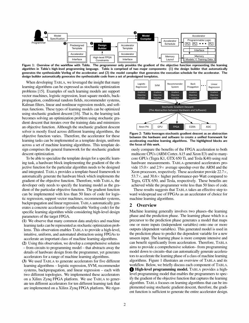
TABLA: A Unified Template-based Framework for

Accelerating Statistical Machine Learning

Divya Mahajan Jongse Park Emmanuel Amaro Hardik Sharma

Amir Yazdanbakhsh Joon Kim Hadi Esmaeilzadeh

Georgia Institute of Technology{divya_mahajan, jspark, amaro, hsharma, a.yazdanbakhsh, jkim796}@gatech.edu hadi@cc.gatech.edu

ABSTRACTA growing number of commercial and enterprise systems increas-ingly rely on compute-intensive machine learning algorithms.While the demand for these compute-intensive applications isgrowing, the performance benefits from general-purpose plat-forms are diminishing. To accommodate the needs of machinelearning algorithms, Field Programmable Gate Arrays (FPGAs)provide a promising path forward and represent an intermediatepoint between the efficiency of ASICs and the programmabilityof general-purpose processors. However, acceleration with FP-GAs still requires long design cycles and extensive expertise inhardware design. To tackle this challenge, instead of designing anaccelerator for machine learning algorithms, we develop TABLA,a framework that generates accelerators for a class of machinelearning algorithms. The key is to identify the commonalitiesacross a wide range of machine learning algorithms and utilizethis commonality to provide a high-level abstraction for program-mers. TABLA leverages the insight that many learning algorithmscan be expressed as stochastic optimization problems. Therefore,a learning task becomes solving an optimization problem usingstochastic gradient descent that minimizes an objective function.The gradient solver is fixed while the objective function changesfor different learning algorithms. TABLA provides a template-based framework for accelerating this class of learning algo-rithms. With TABLA, the developer uses a high-level language toonly specify the learning model as the gradient of the objectivefunction. TABLA then automatically generates the synthesizableimplementation of the accelerator for FPGA realization.

We use TABLA to generate accelerators for ten different learn-ing task that are implemented on a Xilinx Zynq FPGA platform.We rigorously compare the benefits of the FPGA accelerationto both multicore CPUs (ARM Cortex A15 and Xeon E3) andto many-core GPUs (Tegra K1, GTX 650 Ti, and Tesla K40)using real hardware measurements. TABLA-generated acceler-ators provide 15.0⇥ and 2.9⇥ average speedup over the ARMand the Xeon processors, respectively. These accelerator provide22.7⇥, 53.7⇥, and 30.6⇥ higher performance-per-Watt compareto Tegra, GTX 650, and Tesla, respectively. These benefits areachieved while the programmers write less than 50 lines of code.

1 IntroductionA wide range of commercial and enterprise applications suchas mobile health monitoring, social networking, e-commerce,targeted advertising, and financial analysis, increasingly rely onMachine Learning (ML) techniques. In fact, the advances in ma-

chine learning are changing the landscape of computing towardsa more personalized and targeted experience for the users. Forinstance, services that provide personalized health-care and tar-geted advertisement are prevalent or are on the horizon. Machinelearning algorithms are among the computationally intensiveworkloads. Specifically, learning a model from data requiresample amount of computation that is repeated over the trainingdata for a relatively large number of iterations. While the demandfor these computationally intensive techniques increases, the ben-efits from general-purpose computing are diminishing [1, 2]. Asshown in the Dark Silicon study [2] and others corroborate [1, 3],with the effective end of Dennard scaling [4], CMOS scalingis no longer providing performance and efficiency gains thatare commensurate with the transistor density increases [1–3].The current paradigm of general-purpose processor design fallssignificantly short of the traditional cadence of performanceimprovements [5]. These challenges have coincided with theexplosion of data where the rate of data generation has reachedsuch an overwhelming level that is beyond the capabilities ofcurrent computing systems to match [6].

As a result, both the industry and the research community areincreasingly focusing on programmable accelerators, which canprovide large gains in efficiency and performance by restrict-ing the workloads [3, 7–11]. Using FPGAs as programmableaccelerators has the potential for significant performance andefficiency gains while retaining some of the flexibility of general-purpose processors [12]. Commercial parts that incorporate gen-eral purpose cores with programmable logic are beginning toappear [13, 14]. For instance, Microsoft employs FPGAs to ac-celerate their Bing search service [7]. This increasing availabilityof FPGAs for acceleration and their flexibility makes them anattractive platform for accelerating machine learning algorithms.However, a major challenge in using FPGAs is their programma-bility. Development with FPGAs still requires extensive expertisein hardware design and implementation, and the overall designcycle is relatively long even for experts [7]. This paper aims totackle this challenge for an important class of machine learningalgorithms. To this end, we develop TABLA, a template-basedsolution – from circuit to programming model – for using FP-GAs to accelerate statistical machine learning algorithms. Theobjective of our solution is to devise the necessary programmingabstractions and automated frameworks that are uniform acrossa range of machine learning algorithms. TABLA aims to avoidexposing software developers to the details of hardware designby leveraging commonalities in learning algorithms.

Programmer

ModelSpecification

Model Compiler

Design Builder

Predesigned Template

Accelerator

InterfaceHigh-level FPGA

Constraints

Accelerator Template

Accelerator

Interface

Accelerator Schedule

Memory Layout

AcceleratorProgrammable Logic

Interface

MemoryModels Training Data

PU PU PU

1

23

4

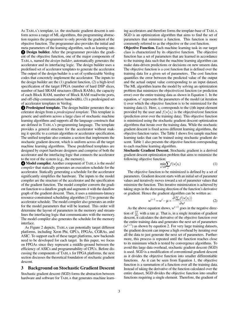
Figure 1: Overview of the workflow with Tabla. The programmer only provides the gradient of the objective function representing the learningalgorithm in Tabla’s high-level programming language. Tabla is comprised of two major components: (1) the design builder that automaticallygenerates the synthesizable Verilog of the accelerator; and (2) the model compiler that generates the execution schedule for the accelerator. Thedesign builder automatically generates the synthesizable code from a set of predesigned templates.

When developing TABLA, we leveraged the insight that manylearning algorithms can be expressed as stochastic optimizationproblems [15]. Examples of such learning models are supportvector machines, logistic regression, least square models, back-propagation, conditional random fields, recommender systems,Kalman filters, linear and nonlinear regression models, and soft-max functions. These types of learning models can be optimizedusing stochastic gradient descent [16]. That is, the learning taskbecomes solving an optimization problem using stochastic gra-dient descent that iterates over the training data and minimizesan objective function. Although the stochastic gradient descentsolver is mostly fixed across different learning algorithms, theobjective function varies. Therefore, the accelerator for theselearning tasks can be implemented as a template design, uniformacross a set of machine learning algorithms. This template de-sign comprises the general framework for the stochastic gradientdescent optimization.

To be able to specialize the template design for a specific learn-ing task, a hardware block implementing the gradient of the ob-jective function for the particular algorithm needs to be designedand integrated. TABLA provides a template-based framework toautomatically generate the hardware block which implements thegradient of the objective function. Therefore, with TABLA, thedeveloper only needs to specify the learning model as the gra-dient of the particular objective function. The gradient functioncan be implemented with less than 50 lines of code for logis-tic regression, support vector machines, recommender systems,backpropagation and linear regression. TABLA automatically gen-erates a concrete accelerator (synthesizable Verilog code) for thespecific learning algorithm while considering high-level designparameters of the target FPGA.(1) We observe that many common data analytics and machinelearning tasks can be represented as stochastic optimization prob-lems. This observation enables TABLA to provide a high-level,intuitive, uniform, and automated abstraction using FPGAs toaccelerate an important class of machine learning algorithms.

(2) Using this observation, we develop a comprehensive solution– from circuits to programming model – that abstracts away thedetails of hardware design from the programmer, yet generatesaccelerators for a range of machine learning algorithms.

(3) We used TABLA to generate accelerators for five differentlearning algorithms – logistic regression, SVM, recommendersystems, backpropagation, and linear regression – each withtwo different topologies. We implemented these acceleratorson a Xilinx Zynq FPGA platform. We use TABLA to gener-ate ten different accelerators for ten different learning task thatare implemented on a Xilinx Zynq FPGA platform. We rigor-

Logis&c(Regression SVM

Stochas&c(Gradient(Descent(The(Abstrac&on(between(Hardware(and(So<ware)

GradientObjec&ve(Func&on

GradientObjec&ve(Func&on

GradientObjec&ve(Func&on

Xeon(Phi GPU FPGA CGRA ASIC

Back(Propga&on

GradientObjec&ve(Func&on

Linear(Regression

GradientObjec&ve(Func&on

Recommender(System

Figure 2: Tabla leverages stochastic gradient descent as an abstractionbetween the hardware and software to create a unified framework foraccelerating machine learning algorithms. The highlighted blocks arethe focus of this work.

ously compare the benefits of the FPGA acceleration to bothmulticore CPUs (ARM Cortex A15 and Xeon E3) and to many-core GPUs (Tegra K1, GTX 650 Ti, and Tesla K40) using realhardware measurements. TABLA-generated accelerators pro-vide 15.0⇥ and 2.9⇥ average speedup over the ARM and theXeon processors, respectively. These accelerator provide 22.7⇥,53.7⇥, and 30.6⇥ higher performance-per-Watt compared toTegra, GTX 650, and Tesla, respectively. These benefits areachieved while the programmer write less than 50 lines of code.

These results suggests that TABLA takes an effective step to-ward widespread use of FPGAs as an accelerator of choice formachine learning algorithms.

2 OverviewMachine learning generally involves two phases–the learningphase and the prediction phase. The learning phase which is aprecursor to the prediction phase generates a model that mapsone or more inputs (independent variables) onto one or moreoutputs (dependent variables). This generated model is used inthe prediction phase to predict the dependent variable for a newunseen input. The learning phase is more compute intensive andcan benefit significantly from acceleration. Therefore, TABLAaims to provide a comprehensive solution– from programmingmodel down to circuits–that can automatically generate accelera-tors to accelerate the learning phase of a class of machine learningalgorithms. Figure 1 illustrates an overview of TABLA and itsworkflow. Below, we briefly discuss each component of TABLA.1 High-level programming model. TABLA provides a high-

level programming model that enables the programmers to spec-ify the gradient of the objective function that captures the learningalgorithm. TABLA focuses on learning algorithms that can be im-plemented using stochastic gradient descent, therefore, the gradi-ent function is sufficient to generate the entire accelerator design.

2

As TABLA’s template, i.e. the stochastic gradient descent is uni-form across a range of ML algorithms, this programming abstrac-tion requires the programmer to only provide the gradient of theobjective function. The programmer also provides the initial andmeta parameters of the learning algorithm, such as learning rate.2 Design builder. After the programmer provides the gradi-

ent of the objective function, one of the major components ofTABLA, named the design builder, automatically generates theaccelerator and its interfacing logic. The design builder uses apredefined set of accelerator templates to generate the accelerator.The output of the design builder is a set of synthesizable Verilogcodes that concretely implement the accelerator. The inputs tothe design builder are the (1) gradient function, (2) a high-levelspecification of the target FPGA (number of hard DSP slices,number of hard SRAM structures (Block RAMs), the capacityof each Block RAM, number of Block RAM read/write ports,and off-chip communication bandwidth), (3) a predesigned setof accelerator templates in Verilog.3 Predesigned template. The design builder generates the ac-

celerator design from a predesigned template. This template isgeneric and uniform across a large class of stochastic machinelearning algorithms and supports all the language constructs thatare defined in TABLA’s programming language. The templateprovides a general structure for the accelerator without mak-ing it specific to a certain algorithm or accelerator specification.The unified template also contains a section that implements thestochastic gradient descent, which is uniform across all the targetmachine learning algorithms. These predefined templates aredesigned by expert hardware designers and comprise of both theaccelerator and the interfacing logic that connects the acceleratorto the rest of the system (e.g., the memory).4 Model compiler. Another component of TABLA is the model

compiler that statically generates an execution schedule for theaccelerator. Statically generating a schedule for the acceleratorsignificantly simplifies the hardware. The inputs to the modelcompiler are the structure of the accelerator and the specificationof the gradient function. The model compiler converts the gradi-ent function to a dataflow graph and augments it with the dataflowgraph of the gradient descent. Then, it uses a minimum-latencyresource-constrained scheduling algorithm [17] to generate theaccelerator schedule. The model compiler also generates an orderfor the model parameters that will be learned. This order willdetermine the layout of parameters in the memory and stream-lines the interfacing logic that communicates with the memory.The model compiler also generates the schedule for the memoryinterface.

As Figure 2 depicts, TABLA can potentially target differentplatforms, including Xeon Phi, GPUs, FPGAs, CGRAs, andASIC. To support each of these target platforms, new backendsneed to be developed for each target. In this paper, we focuson FPGAs since they represent a middle-ground between theefficiency of ASICs and programmability of CPUs. Before dis-cussing the components of TABLA for FPGA platforms, the nextsection discusses the theoretical foundation of stochastic gradientdescent.

3 Background on Stochastic Gradient DescentStochastic gradient descent (SGD) forms the abstraction betweenhardware and software for TABLA that generates machine learn-

ing accelerators and therefore forms the template-base of TABLA.SGD is an optimization algorithm that aims to find the set ofparameters that minimize a function. This function is morecommonly referred to as the objective or the cost function.Objective Function. Each machine learning task in our targetclass is characterized by its objective function. The objectivefunction has a set of parameters that are learned in accordanceto the training data such that the machine learning algorithm canmake data-driven predictions or decisions on new unseen data.The objective function is a cost function that is defined over thetraining data for a given set of parameters. The cost functionquantifies the error between the predicted value of the outputand the actual output value corresponding to an input dataset.The ML algorithm learns the model by solving an optimizationproblem that minimizes the objective/cost function (or predictionerror) over the entire training data as shown in Equation 1. In theequation, wt represents the parameters of the model (at iterationt) over which the objective function is to be minimized for thetraining data (i). Here, xi corresponds to the (i)th input elementprovided by the user and f (wt

ixi) is the objective/cost function(prediction error over the training data). This objective functionis minimized using the stochastic gradient descent optimizationalgorithms that iterate over the training data. While the stochasticgradient descent is fixed across different learning algorithms, theobjective function varies. The Table 1 shows five sample machinelearning tasks that can be trained using stochastic gradient de-scent. Table 1 also presents the objective function correspondingto each machine learning algorithm.Stochastic Gradient Descent. Stochastic gradient is a derivedgradient descent optimization problem that aims to minimize thefollowing objective function:

minwteR

Âi

f (wtixi) (1)

The objective function to be minimized is defined by a set ofparameters. Gradient descent starts with an initial set of parametervalues and iteratively moves toward a set of parameter values thatminimize the function. This iterative minimization is achieved bytaking steps in the decreasing direction of the function’s derivativeor gradient. Hence the gradient algorithm can be written as:

wt+1=wt�µ⇥ ∂(Âi f (wtixi))

∂wt (2)

As the above equation shows, wt+1 goes in the negative direc-tion of ∂ f

∂w with a rate µ. That is, in a single iteration of gradientdescent, it calculates the derivative of the objective function overthe entire training data and generates the next set of parameters(wt+1) as shown by equation 2. For very large training datasets,the gradient descent can impose a high overhead by iterating overall the data to just generate the next set of parameters. Further-more, this process is repeated until the function reaches closeto its minimum which is tested by convergence algorithms. Toavoid this large data overhead, stochastic gradient descent (SGD)is used. SGD is a modification of conventional gradient descentas it divides the objective function into smaller differentiablefunctions. As it can be seen from Equation 1, the objectivefunction is a summation of a function over all the training data.Instead of taking the derivative of the function calculated over theentire dataset, SGD divides the objective function into smallerfunctions requiring a single element. Therefore, the gradient of

3

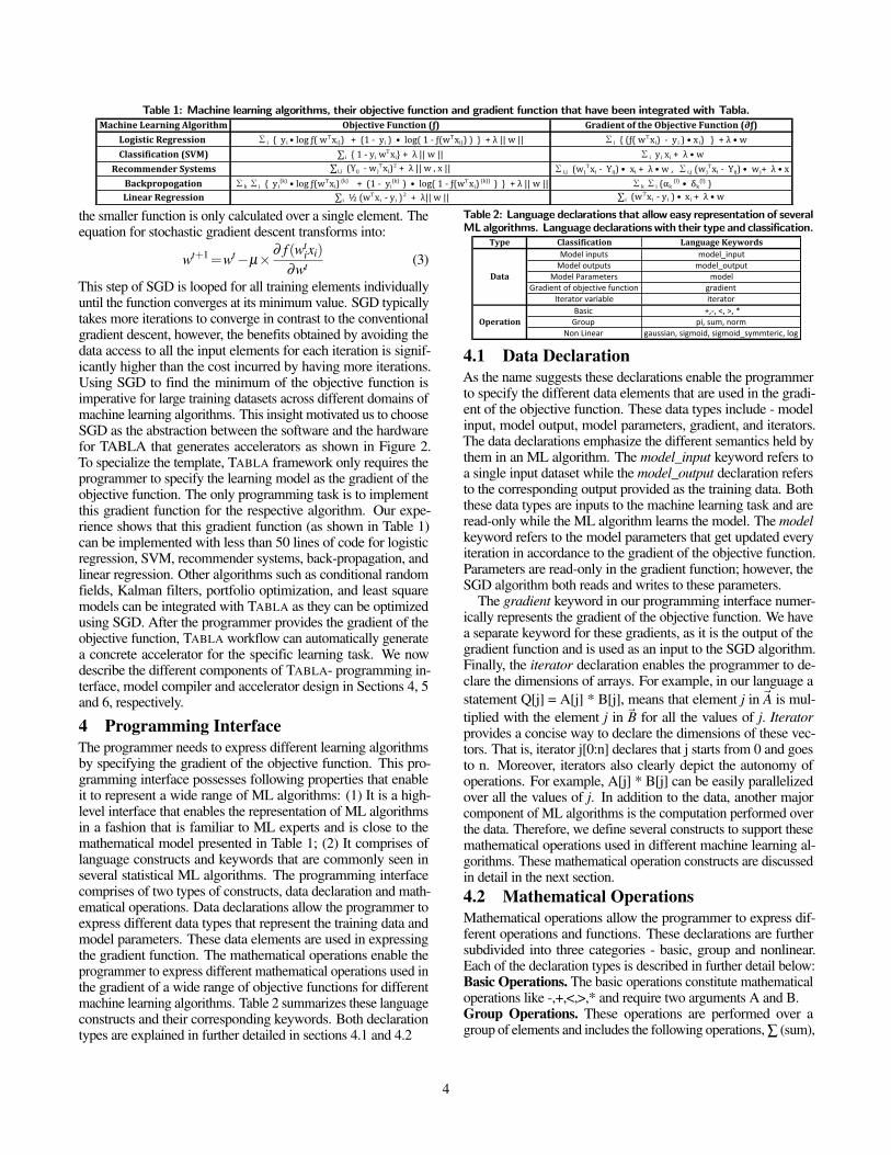
Table 1: Machine learning algorithms, their objective function and gradient function that have been integrated with Tabla.Machine(Learning(Algorithm Objective(Function((ƒ) Gradient(of(the(Objective(Function((∂ƒ)

Logistic(Regression( �i""{""yi"•"log"ƒ("wTxi))"""+""(1"1""yi")""•""log("1"1"ƒ(wTxi))")""}""+"λ"||"w"|| �i""{"(ƒ("wTxi)""1""yi")"•"xi)"""}""+"λ"•"wClassification((SVM) ∑i""{"1"1"yi"wTxi}"+""λ"||"w"|| �i""yi"xi"+""λ"•"w

Recommender(Systems ∑i,j""(Yij""1"wjTxi)2"+""λ"||"w","x"|| �i,j ""(wj

Txi""1""Yij)"•" "xi"+""λ"•"w",""�i,j "(wjTxi""1""Yij)"•" "wj+""λ"•"x

Backpropogation �k"�i""{""yi(k) "•"log"ƒ(wTxi)"(k) """"+""(1"1""yi(k)"")" "•""log("1"1"ƒ(wTxi)"(k))"")""}""+"λ"||"w"|| �k"�i"(αk"(l) "•""δk(l) ")Linear(Regression ∑i""½"(wTxi"" 1"yi")2""+""λ||"w"|| ∑i""(wTxi"" 1"yi")"•""xi"+""λ"•"w"

the smaller function is only calculated over a single element. Theequation for stochastic gradient descent transforms into:

wt+1=wt�µ⇥ ∂ f (wtixi)

∂wt (3)

This step of SGD is looped for all training elements individuallyuntil the function converges at its minimum value. SGD typicallytakes more iterations to converge in contrast to the conventionalgradient descent, however, the benefits obtained by avoiding thedata access to all the input elements for each iteration is signif-icantly higher than the cost incurred by having more iterations.Using SGD to find the minimum of the objective function isimperative for large training datasets across different domains ofmachine learning algorithms. This insight motivated us to chooseSGD as the abstraction between the software and the hardwarefor TABLA that generates accelerators as shown in Figure 2.To specialize the template, TABLA framework only requires theprogrammer to specify the learning model as the gradient of theobjective function. The only programming task is to implementthis gradient function for the respective algorithm. Our expe-rience shows that this gradient function (as shown in Table 1)can be implemented with less than 50 lines of code for logisticregression, SVM, recommender systems, back-propagation, andlinear regression. Other algorithms such as conditional randomfields, Kalman filters, portfolio optimization, and least squaremodels can be integrated with TABLA as they can be optimizedusing SGD. After the programmer provides the gradient of theobjective function, TABLA workflow can automatically generatea concrete accelerator for the specific learning task. We nowdescribe the different components of TABLA- programming in-terface, model compiler and accelerator design in Sections 4, 5and 6, respectively.

4 Programming InterfaceThe programmer needs to express different learning algorithmsby specifying the gradient of the objective function. This pro-gramming interface possesses following properties that enableit to represent a wide range of ML algorithms: (1) It is a high-level interface that enables the representation of ML algorithmsin a fashion that is familiar to ML experts and is close to themathematical model presented in Table 1; (2) It comprises oflanguage constructs and keywords that are commonly seen inseveral statistical ML algorithms. The programming interfacecomprises of two types of constructs, data declaration and math-ematical operations. Data declarations allow the programmer toexpress different data types that represent the training data andmodel parameters. These data elements are used in expressingthe gradient function. The mathematical operations enable theprogrammer to express different mathematical operations used inthe gradient of a wide range of objective functions for differentmachine learning algorithms. Table 2 summarizes these languageconstructs and their corresponding keywords. Both declarationtypes are explained in further detailed in sections 4.1 and 4.2

Table 2: Language declarations that allow easy representation of severalMLalgorithms. Language declarationswith their type and classification.

Type Classification Language2KeywordsModel&inputs model_inputModel&outputs model_output

Model&Parameters modelGradient&of&objective&function gradient

Iterator&variable iteratorBasic& &+,=,&<,&>,&*Group& pi,&sum,&norm

Non&Linear& gaussian,&sigmoid,&sigmoid_symmteric,&log

Data

Operation

4.1 Data DeclarationAs the name suggests these declarations enable the programmerto specify the different data elements that are used in the gradi-ent of the objective function. These data types include - modelinput, model output, model parameters, gradient, and iterators.The data declarations emphasize the different semantics held bythem in an ML algorithm. The model_input keyword refers toa single input dataset while the model_output declaration refersto the corresponding output provided as the training data. Boththese data types are inputs to the machine learning task and areread-only while the ML algorithm learns the model. The modelkeyword refers to the model parameters that get updated everyiteration in accordance to the gradient of the objective function.Parameters are read-only in the gradient function; however, theSGD algorithm both reads and writes to these parameters.

The gradient keyword in our programming interface numer-ically represents the gradient of the objective function. We havea separate keyword for these gradients, as it is the output of thegradient function and is used as an input to the SGD algorithm.Finally, the iterator declaration enables the programmer to de-clare the dimensions of arrays. For example, in our language astatement Q[j] = A[j] * B[j], means that element j in~A is mul-tiplied with the element j in ~B for all the values of j. Iteratorprovides a concise way to declare the dimensions of these vec-tors. That is, iterator j[0:n] declares that j starts from 0 and goesto n. Moreover, iterators also clearly depict the autonomy ofoperations. For example, A[j] * B[j] can be easily parallelizedover all the values of j. In addition to the data, another majorcomponent of ML algorithms is the computation performed overthe data. Therefore, we define several constructs to support thesemathematical operations used in different machine learning al-gorithms. These mathematical operation constructs are discussedin detail in the next section.4.2 Mathematical OperationsMathematical operations allow the programmer to express dif-ferent operations and functions. These declarations are furthersubdivided into three categories - basic, group and nonlinear.Each of the declaration types is described in further detail below:Basic Operations. The basic operations constitute mathematicaloperations like -,+,<,>,* and require two arguments A and B.Group Operations. These operations are performed over agroup of elements and includes the following operations, Â (sum),

4

P (group multiply), and || || (norm). The pi and sum keywordstake in two arguments while the norm keyword only takes one.Apart from the input values, these operation types require aniterator argument to operate on a group of elements.

As these operations process groups of elements, they producean output with dimension one less than the input dimension. Forinstance, operating on a vector input produces a scalar output.Nonlinear Operations. These operations constitute nonlinearfunctions like Log, Sigmoid, Gaussian, and Sigmoid Symmet-ric. The output has the same dimensionality as the input as thisoperation is performed element by element.

Using the data and operation language declarations definedabove, programmer can easily represent several statistical MLalgorithms. One such example is Logistic Regression. Thefollowing code shows how the gradient of logistic regression(given in Table 1) can be expressed in a few lines using TABLA’sprogramming interface.m o d e l _ i n p u t x[m]; // model input features

m o d e l _ o u t p u t y’[n]; // model outputs

model w[n][m]; // model parameters

g r a d i e n t g[n][m]; // gradient

i t e r a t o r i[0:m]; // iterator for group operations

i t e r a t o r j[0:n]; // iterator for group operations

//m parallel multiplications followed by

// an addition tree; repeat n times in parallel

s[j] = sum[i](x[i] * w[j][i]);

y[j] = sigmoid(s[j]) ; //n parallel sigmoid operations

e[j] = y[j] - y’[j]; //n parallel subtractions

g[j][i] = x[i] * e[j]; // n*m parallel multiplications

rg[j][i] = l * w[i][j]; // n*m parallel multiplications

g[j][i] = g[j][i] + rg[j][i]; // n*m parallel additions

The above code shows the simplicity of our programminginterface and expresses a complicated mathematical function ofthe gradient of the objective function into smaller and much sim-pler operations. In this code the programmer first declares thedata types: model_input, model_output, model and the gradi-ent. Then, two iterators i and j are declared as the model valuesare two dimensional. Next, operations are performed over thedeclared data types beginning with the sum operation. This op-eration performs multiplication x[i] * w[j][i] and adds up all themultiplication results into a single result (s[j]) in the i dimensionassuming a constant j. On the other hand, the left hand side of thestatement s[j] shows that the summation operation is repeated ntimes using the j iterator. By following a similar concept wherethe iterator on the LHS of the equation signifies a loop over thatiterator variable, other operations are also performed. Finallythe result generated by this code is the gradient for the givenmodel_input, model_output and model.

Several ML algorithms can be represented using the abovementioned language declarations. The simplicity of these decla-rations to express mathematical models makes the programminginterface easy to use. Furthermore, the programming interfacecan be extended to incorporate more declarations so as to accom-modate the representation of an even wider range of statisticalML algorithms.

Although MATLAB and R can also be used to represent thesame ML algorithms, we designed and used TABLA’s in-houseprogramming interface due to the following reasons: (1) easierrepresentation of gradient functions using the common mathemat-ical constructs used in ML; (2) ease in identifying parts of code

that can be made parallel; (3) convenient conversion of gradientfunction into the final hardware design using the model compilerdescribed in the Section 5;

In the next section we detail the flow of the model compilerwhich illustrates how the gradient of the objective function pro-vided by the programmer using our language declarations canbe appended with the stochastic gradient descent. Furthermore,the model compiler also has the responsibility of converting theunified objective function gradient and SGD into a data-flowgraph and finally into a schedule that can be mapped onto thehardware design.

5 Model Compiler for TABLA

After the programmer provides the gradient of the objectivefunction, TABLA’s model compiler first integrates this objectivefunction with the stochastic gradient descent. To generate a con-crete accelerator, the model compiler then generates a dataflowgraph that can be mapped and scheduled on hardware. Dataflowgraphs (DFGs) are intermediate representations that can be trans-lated into the accelerator and its execution schedule. Thus, thefinal phase of compilation is the scheduling phase in which thecompiler generates a static schedule for the learning task that isrepresented by a dataflow graph.5.1 Integration of Stochastic Gradient DescentAn optimization algorithm is required to solve a machine learningtask. The target is to find the minimum value of the objectivefunction corresponding to the learning task. To solve this task,the programmer provides the gradient of the cost function andTABLA subsequently uses stochastic gradient descent as the op-timization algorithm to determine the parameters best suited forthe given training data. Since SGD is independent of the learningtask, we devise a general template to implement it. As a result,we need a mechanism to integrate the gradient of the objectivefunction with our template.

As seen in Section 4, the programmer provided code generatesa final result, which is the gradient of the cost function and is rep-resented using the gradient argument. Stochastic gradient descentis then executed using this gradient result and model declarationsprovided by the programmer using the following code:model w[n][m]; // model parameters

g r a d i e n t g[n][m]; // gradient

g[j][i] = µ * g[j][i] // n*m parallel multiplications

g[j][i] = w[j][i] -g[j][i]; // n*m parallel subtractions

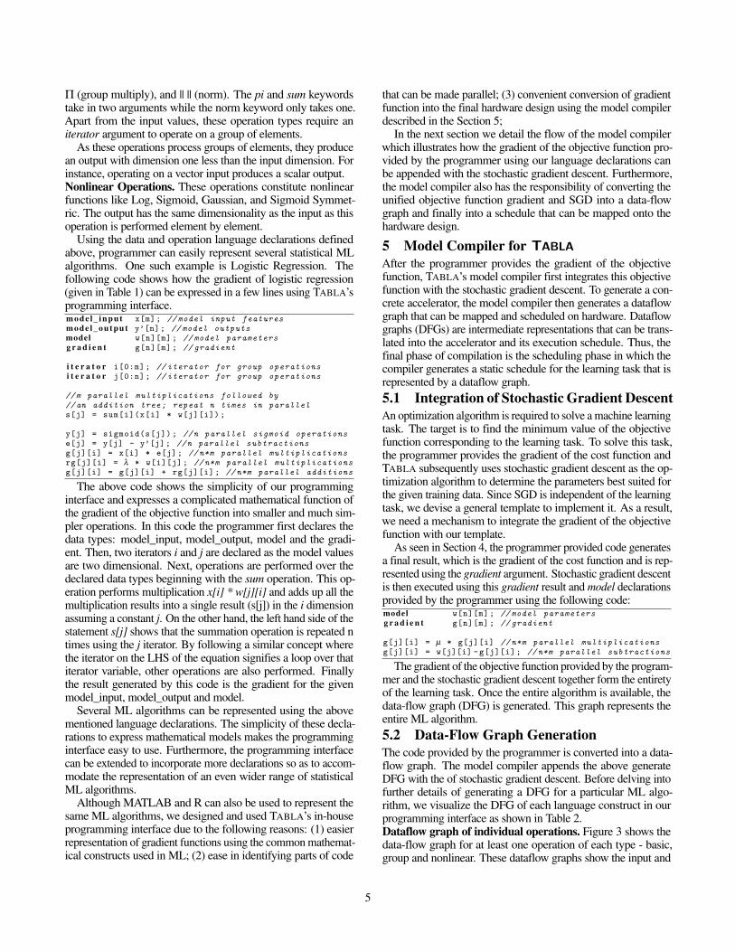
The gradient of the objective function provided by the program-mer and the stochastic gradient descent together form the entiretyof the learning task. Once the entire algorithm is available, thedata-flow graph (DFG) is generated. This graph represents theentire ML algorithm.5.2 Data-Flow Graph GenerationThe code provided by the programmer is converted into a data-flow graph. The model compiler appends the above generateDFG with the of stochastic gradient descent. Before delving intofurther details of generating a DFG for a particular ML algo-rithm, we visualize the DFG of each language construct in ourprogramming interface as shown in Table 2.Dataflow graph of individual operations. Figure 3 shows thedata-flow graph for at least one operation of each type - basic,group and nonlinear. These dataflow graphs show the input and

5

Basic Group Nonlinear

Multiply

** *

+* *

+

+

Sigmoid* *

+* *

+

+Sum Norm Sigmoid

Figure 3: Dataflow graph for basic, group and nonlinear type ofoperations. The DFG for multiply, sum, norm and sigmoid operationsare shown.

* *+

* *+

+

...

...

x[0] w[0] x[m] w[m]...

...* *w[m]

rg[0] rg[m]

Sigmoid

—

...* * *x[m-1]

*x[1]x[0]

+ + + +

* * * *µ µµµ

— — — —

...

...

...

Programmer'sCode

StochasticGradient Descent

Sum[i](w[i] * x[i])

x[m]

rg[m-1]rg[1]rg[0] rg[m]

w[m-1]w[1]w[0] w[m]

w[0]λ λ

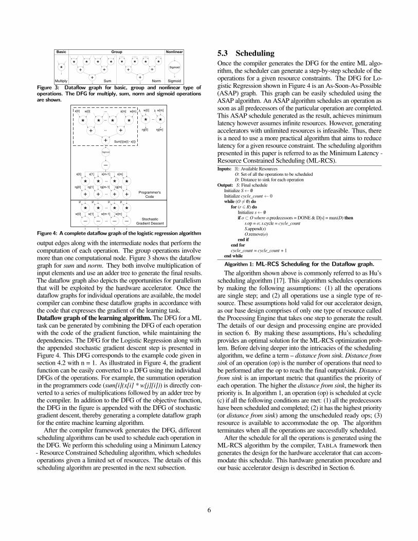
Figure 4: A complete dataflow graph of the logistic regression algorithm

output edges along with the intermediate nodes that perform thecomputation of each operation. The group operations involvemore than one computational node. Figure 3 shows the dataflowgraph for sum and norm. They both involve multiplication ofinput elements and use an adder tree to generate the final results.The dataflow graph also depicts the opportunities for parallelismthat will be exploited by the hardware accelerator. Once thedataflow graphs for individual operations are available, the modelcompiler can combine these dataflow graphs in accordance withthe code that expresses the gradient of the learning task.Dataflow graph of the learning algorithm. The DFG for a MLtask can be generated by combining the DFG of each operationwith the code of the gradient function, while maintaining thedependencies. The DFG for the Logistic Regression along withthe appended stochastic gradient descent step is presented inFigure 4. This DFG corresponds to the example code given insection 4.2 with n = 1. As illustrated in Figure 4, the gradientfunction can be easily converted to a DFG using the individualDFGs of the operations. For example, the summation operationin the programmers code (sum[i](x[i] * w[j][i])) is directly con-verted to a series of multiplications followed by an adder tree bythe compiler. In addition to the DFG of the objective function,the DFG in the figure is appended with the DFG of stochasticgradient descent, thereby generating a complete dataflow graphfor the entire machine learning algorithm.

After the compiler framework generates the DFG, differentscheduling algorithms can be used to schedule each operation inthe DFG. We perform this scheduling using a Minimum Latency- Resource Constrained Scheduling algorithm, which schedulesoperations given a limited set of resources. The details of thisscheduling algorithm are presented in the next subsection.

5.3 SchedulingOnce the compiler generates the DFG for the entire ML algo-rithm, the scheduler can generate a step-by-step schedule of theoperations for a given resource constraints. The DFG for Lo-gistic Regression shown in Figure 4 is an As-Soon-As-Possible(ASAP) graph. This graph can be easily scheduled using theASAP algorithm. An ASAP algorithm schedules an operation assoon as all predecessors of the particular operation are completed.This ASAP schedule generated as the result, achieves minimumlatency however assumes infinite resources. However, generatingaccelerators with unlimited resources is infeasible. Thus, thereis a need to use a more practical algorithm that aims to reducelatency for a given resource constraint. The scheduling algorithmpresented in this paper is referred to as the Minimum Latency -Resource Constrained Scheduling (ML-RCS).Inputs: R: Available Resources

O: Set of all the operations to be scheduledD: Distance to sink for each operation

Output: S: Final scheduleInitialize S /0Initialize cycle_count 0while (O 6= /0) do

for (r 2 R) doInitialize s /0if o⇢ O where o.predecessors = DONE & D[s] = max(D) then

s.op = o; s.cycle = cycle_countS.append(s)O.remove(o)

end ifend forcycle_count = cycle_count + 1

end while

Algorithm 1: ML-RCS Scheduling for the Dataflow graph.

The algorithm shown above is commonly referred to as Hu’sscheduling algorithm [17]. This algorithm schedules operationsby making the following assumptions: (1) all the operationsare single step; and (2) all operations use a single type of re-source. These assumptions hold valid for our accelerator design,as our base design comprises of only one type of resource calledthe Processing Engine that takes one step to generate the result.The details of our design and processing engine are providedin section 6. By making these assumptions, Hu’s schedulingprovides an optimal solution for the ML-RCS optimization prob-lem. Before delving deeper into the intricacies of the schedulingalgorithm, we define a term – distance from sink. Distance fromsink of an operation (op) is the number of operations that need tobe performed after the op to reach the final output/sink. Distancefrom sink is an important metric that quantifies the priority ofeach operation. The higher the distance from sink, the higher itspriority is. In algorithm 1, an operation (op) is scheduled at cycle(c) if all the following conditions are met: (1) all the predecessorshave been scheduled and completed; (2) it has the highest priority(or distance from sink) among the unscheduled ready ops; (3)resource is available to accommodate the op. The algorithmterminates when all the operations are successfully scheduled.

After the schedule for all the operations is generated using theML-RCS algorithm by the compiler, TABLA framework thengenerates the design for the hardware accelerator that can accom-modate this schedule. This hardware generation procedure andour basic accelerator design is described in Section 6.

6

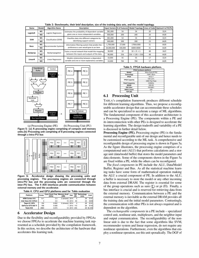
Table 3: Benchmarks, their brief description, size of the training data sets, and the model topology.Name Model Algorithm/Name Description Input/Vectors #/of/Features Model/Topology Lines/of/Code Optimal/#/of/PE/PU

M1 581,000 54 54 20 32/4

M2 500,000 200 200 20 64/8

M1 581,000 54 54 23 32/4

M2 500,000 200 200 23 64/8

M1 1,700,000 27,000 1700x1000 31 64/8

M2 24,000,000 100,000 6000×4000 31 64/8

M1 38,000 10 10./>.9./>.1 48 16/2

M2 90,000 256 256./>.128./>.256 48 64/8

M1 10,000 55 55 17 32/4

M2 10,000 784 784 17 64/8

Reco/

LogisticR/

SVM

Backprop

LinearR Linear.RegressionModels.relationship.between.a.dependent.

variable.and.one.or.more.explanatory.variables.

Information.filtering.system.that.predict.the.preference.a.user.would.give.to.an.item

Classifies.data.into.different.categories.by.identifying.support.vectors.

Logistic.Regression.Estimates.the.probability.of.dependent.variable.

given.one.or.more.independent.variables

BackpropogationTrains.a.neural.network.that.model.the.mapping.between.the.inputs.and.outputs.of.the.data

Recommender.Systems

Classification.(SVM)

NeighborInput

Register

NonlinearUnit

Register

Control

Neighboroutput

Bus Input/Output

Data/ModelBuffer

(a) Processing Engine (PE)

PE 4

Global BusInput/Output

Bus Scheduler

PE 3

PE 5 PE 2

PE 6 PE 1

PE 7 PE 0

(b) Processing Unit (PU)Figure 5: (a) A processing engine comprising of compute and memoryunits.(b) Processing unit comprising of 8 processing engines connectedthrough a intra-PU bus

PE0 PE1 PE6 PE7

Con

trol...

PE0 PE1 PE6 PE7

Con

trol...

...

PE0 PE1 PE6 PE7

Con

trol...

Buf

fer

AX

I Mas

ter

Inte

rfac

e

Ext

erna

l Mem

ory

Figure 6: Accelerator design showing the processing units andprocessing engines. The processing engines are connected throughintra-PU bus and the processing units are connected through theinter-PU bus. The 4 AXI interfaces provide communication betweenexternal memory and the accelerator.

Table 4: CPU and GPU platforms used for Tabla evaluation

Platform Cores Core Clock Freq (GHz)

Memory Avail (GB) Year TDP

(W)Technology

(nm) Cost

ARM Cortex A15 4+1 2.3 2 (shared) 2014 5 28 $191Intel Xeon E3-1276v3 4 3.6 16 2014 84 22 $339

Tegra K1 GPU 192 0.852 2 (shared) 2014 5 28 $191 GeForce GTX 650 Ti 768 0.928 1 2012 110 28 $150

Tesla K40 2880 0.875 12 2013 235 28 $5,499

6 Accelerator DesignDue to the flexibility and reconfigurability provided by FPGAswe choose FPGAs to accelerate the machine learning task rep-resented as a schedule provided by the compilation framework.In this section, we describe the architecture of the hardware thataccelerates this learning task.

Table 5: FPGA hardware platform.

Model Xilinx&Zynq&ZC702Technology TSMC&28nm

FPGA Artix6753K&LUTs

106K&Flip6FlopsPeak2Frequency 250MHz

BRAM 630&KBDSP2Slice DSP48E1

MACC2Count 220TDP2(W) 2

FPGA2hardware2platform

FPGA2Capacity

6.1 Processing UnitTABLA’s compilation framework produces different schedulefor different learning algorithms. Thus, we propose a reconfig-urable accelerator design that can accommodate these schedulesand can be specialized to accelerate a range of ML algorithms.The fundamental component of this accelerator architecture isa Processing Engine (PE). The components within a PE andits interconnection with other PEs is designed to accelerate thelearning algorithm. The design tradeoffs and variability of a PEis discussed in further detail below.Processing Engine (PE). Processing engine (PE) is the funda-mental and reconfigurable unit of our design and hence needs tobe customized according to the ML task. A comprehensive andreconfigurable design of processing engine is shown in Figure 5a.As the figure illustrates, the processing engine comprises of acomputational unit (ALU) that performs calculations and a stor-age unit (data/model buffer) that stores the model parameters anddata elements. Some of the components shown in the Figure 5aare fixed within a PE, while the others can be reconfigured.

The fixed components in PE include the ALU, Data/ModelBuffer, Register and Bus. As all the statistical machine learn-ing tasks have some form of mathematical operation makingthe ALU a crucial component of PE. In addition to the ALU,a buffer is necessary to store the model or any other incomingdata from external DRAM. The register is essential for someof the group operations such as sum (Â) or pi (P). Finally, abus interface is crucial and is reserved for retrieving data fromthe external memory. Communication between a PE and theexternal memory is inevitable as the external DRAM provides allthe training data and the initial model parameters. Contrastingly,the communication with other PEs is not always required and isdependent on the algorithm.

The exchangeable components in a PE include – specializedcontrol unit, nonlinear unit, multiplexers, and the neighbor inputand output communication. The reconfigurability of the non-linear unit is due to the fact that some algorithms like SVM,recommender system and linear regression, do not require anynonlinear operations. Furthermore, even the algorithms that em-ploy a nonlinear operation, use this unit sporadically. The DGF of

7

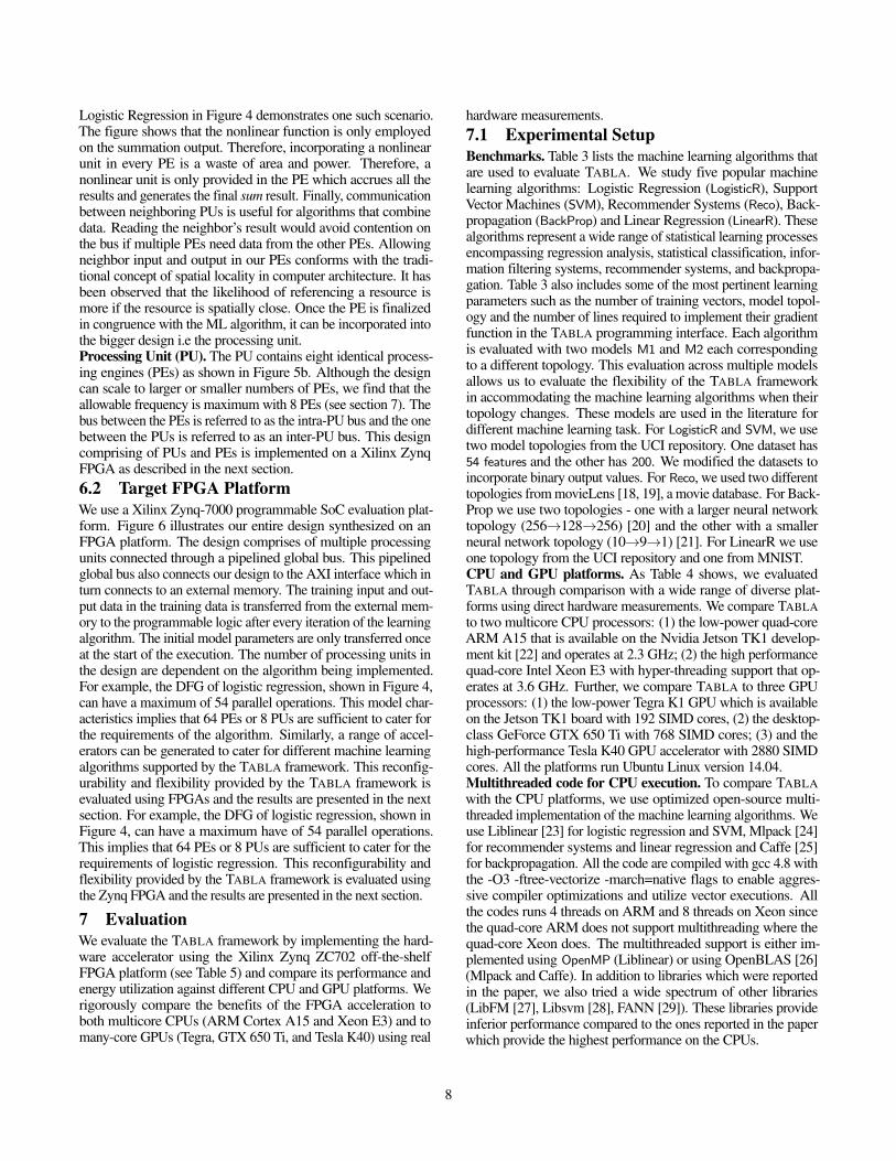
Logistic Regression in Figure 4 demonstrates one such scenario.The figure shows that the nonlinear function is only employedon the summation output. Therefore, incorporating a nonlinearunit in every PE is a waste of area and power. Therefore, anonlinear unit is only provided in the PE which accrues all theresults and generates the final sum result. Finally, communicationbetween neighboring PUs is useful for algorithms that combinedata. Reading the neighbor’s result would avoid contention onthe bus if multiple PEs need data from the other PEs. Allowingneighbor input and output in our PEs conforms with the tradi-tional concept of spatial locality in computer architecture. It hasbeen observed that the likelihood of referencing a resource ismore if the resource is spatially close. Once the PE is finalizedin congruence with the ML algorithm, it can be incorporated intothe bigger design i.e the processing unit.Processing Unit (PU). The PU contains eight identical process-ing engines (PEs) as shown in Figure 5b. Although the designcan scale to larger or smaller numbers of PEs, we find that theallowable frequency is maximum with 8 PEs (see section 7). Thebus between the PEs is referred to as the intra-PU bus and the onebetween the PUs is referred to as an inter-PU bus. This designcomprising of PUs and PEs is implemented on a Xilinx ZynqFPGA as described in the next section.6.2 Target FPGA PlatformWe use a Xilinx Zynq-7000 programmable SoC evaluation plat-form. Figure 6 illustrates our entire design synthesized on anFPGA platform. The design comprises of multiple processingunits connected through a pipelined global bus. This pipelinedglobal bus also connects our design to the AXI interface which inturn connects to an external memory. The training input and out-put data in the training data is transferred from the external mem-ory to the programmable logic after every iteration of the learningalgorithm. The initial model parameters are only transferred onceat the start of the execution. The number of processing units inthe design are dependent on the algorithm being implemented.For example, the DFG of logistic regression, shown in Figure 4,can have a maximum of 54 parallel operations. This model char-acteristics implies that 64 PEs or 8 PUs are sufficient to cater forthe requirements of the algorithm. Similarly, a range of accel-erators can be generated to cater for different machine learningalgorithms supported by the TABLA framework. This reconfig-urability and flexibility provided by the TABLA framework isevaluated using FPGAs and the results are presented in the nextsection. For example, the DFG of logistic regression, shown inFigure 4, can have a maximum have of 54 parallel operations.This implies that 64 PEs or 8 PUs are sufficient to cater for therequirements of logistic regression. This reconfigurability andflexibility provided by the TABLA framework is evaluated usingthe Zynq FPGA and the results are presented in the next section.

7 EvaluationWe evaluate the TABLA framework by implementing the hard-ware accelerator using the Xilinx Zynq ZC702 off-the-shelfFPGA platform (see Table 5) and compare its performance andenergy utilization against different CPU and GPU platforms. Werigorously compare the benefits of the FPGA acceleration toboth multicore CPUs (ARM Cortex A15 and Xeon E3) and tomany-core GPUs (Tegra, GTX 650 Ti, and Tesla K40) using real

hardware measurements.7.1 Experimental SetupBenchmarks. Table 3 lists the machine learning algorithms thatare used to evaluate TABLA. We study five popular machinelearning algorithms: Logistic Regression (LogisticR), SupportVector Machines (SVM), Recommender Systems (Reco), Back-propagation (BackProp) and Linear Regression (LinearR). Thesealgorithms represent a wide range of statistical learning processesencompassing regression analysis, statistical classification, infor-mation filtering systems, recommender systems, and backpropa-gation. Table 3 also includes some of the most pertinent learningparameters such as the number of training vectors, model topol-ogy and the number of lines required to implement their gradientfunction in the TABLA programming interface. Each algorithmis evaluated with two models M1 and M2 each correspondingto a different topology. This evaluation across multiple modelsallows us to evaluate the flexibility of the TABLA frameworkin accommodating the machine learning algorithms when theirtopology changes. These models are used in the literature fordifferent machine learning task. For LogisticR and SVM, we usetwo model topologies from the UCI repository. One dataset has54 features and the other has 200. We modified the datasets toincorporate binary output values. For Reco, we used two differenttopologies from movieLens [18, 19], a movie database. For Back-Prop we use two topologies - one with a larger neural networktopology (256!128!256) [20] and the other with a smallerneural network topology (10!9!1) [21]. For LinearR we useone topology from the UCI repository and one from MNIST.CPU and GPU platforms. As Table 4 shows, we evaluatedTABLA through comparison with a wide range of diverse plat-forms using direct hardware measurements. We compare TABLAto two multicore CPU processors: (1) the low-power quad-coreARM A15 that is available on the Nvidia Jetson TK1 develop-ment kit [22] and operates at 2.3 GHz; (2) the high performancequad-core Intel Xeon E3 with hyper-threading support that op-erates at 3.6 GHz. Further, we compare TABLA to three GPUprocessors: (1) the low-power Tegra K1 GPU which is availableon the Jetson TK1 board with 192 SIMD cores, (2) the desktop-class GeForce GTX 650 Ti with 768 SIMD cores; (3) and thehigh-performance Tesla K40 GPU accelerator with 2880 SIMDcores. All the platforms run Ubuntu Linux version 14.04.Multithreaded code for CPU execution. To compare TABLAwith the CPU platforms, we use optimized open-source multi-threaded implementation of the machine learning algorithms. Weuse Liblinear [23] for logistic regression and SVM, Mlpack [24]for recommender systems and linear regression and Caffe [25]for backpropagation. All the code are compiled with gcc 4.8 withthe -O3 -ftree-vectorize -march=native flags to enable aggres-sive compiler optimizations and utilize vector executions. Allthe codes runs 4 threads on ARM and 8 threads on Xeon sincethe quad-core ARM does not support multithreading where thequad-core Xeon does. The multithreaded support is either im-plemented using OpenMP (Liblinear) or using OpenBLAS [26](Mlpack and Caffe). In addition to libraries which were reportedin the paper, we also tried a wide spectrum of other libraries(LibFM [27], Libsvm [28], FANN [29]). These libraries provideinferior performance compared to the ones reported in the paperwhich provide the highest performance on the CPUs.

8

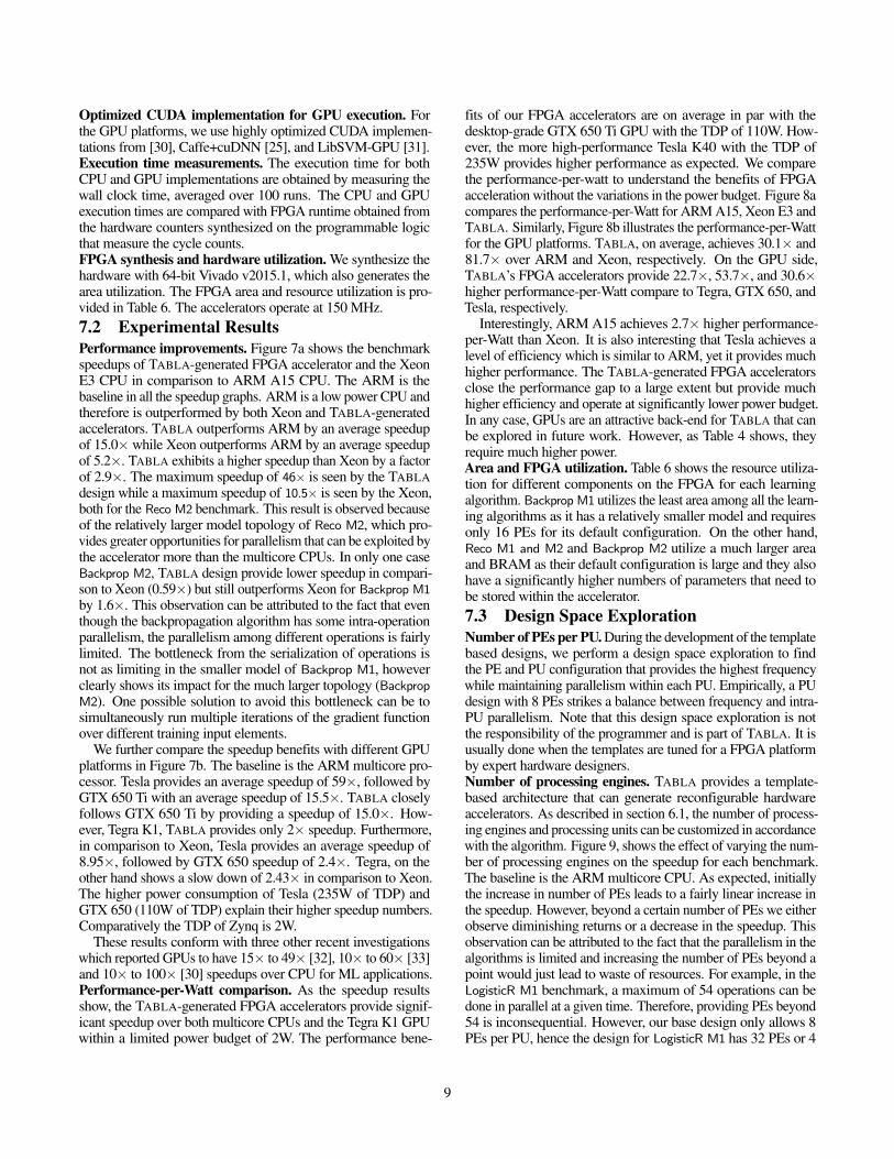
Optimized CUDA implementation for GPU execution. Forthe GPU platforms, we use highly optimized CUDA implemen-tations from [30], Caffe+cuDNN [25], and LibSVM-GPU [31].Execution time measurements. The execution time for bothCPU and GPU implementations are obtained by measuring thewall clock time, averaged over 100 runs. The CPU and GPUexecution times are compared with FPGA runtime obtained fromthe hardware counters synthesized on the programmable logicthat measure the cycle counts.FPGA synthesis and hardware utilization. We synthesize thehardware with 64-bit Vivado v2015.1, which also generates thearea utilization. The FPGA area and resource utilization is pro-vided in Table 6. The accelerators operate at 150 MHz.7.2 Experimental ResultsPerformance improvements. Figure 7a shows the benchmarkspeedups of TABLA-generated FPGA accelerator and the XeonE3 CPU in comparison to ARM A15 CPU. The ARM is thebaseline in all the speedup graphs. ARM is a low power CPU andtherefore is outperformed by both Xeon and TABLA-generatedaccelerators. TABLA outperforms ARM by an average speedupof 15.0⇥ while Xeon outperforms ARM by an average speedupof 5.2⇥. TABLA exhibits a higher speedup than Xeon by a factorof 2.9⇥. The maximum speedup of 46⇥ is seen by the TABLAdesign while a maximum speedup of 10.5⇥ is seen by the Xeon,both for the Reco M2 benchmark. This result is observed becauseof the relatively larger model topology of Reco M2, which pro-vides greater opportunities for parallelism that can be exploited bythe accelerator more than the multicore CPUs. In only one caseBackprop M2, TABLA design provide lower speedup in compari-son to Xeon (0.59⇥) but still outperforms Xeon for Backprop M1by 1.6⇥. This observation can be attributed to the fact that eventhough the backpropagation algorithm has some intra-operationparallelism, the parallelism among different operations is fairlylimited. The bottleneck from the serialization of operations isnot as limiting in the smaller model of Backprop M1, howeverclearly shows its impact for the much larger topology (BackpropM2). One possible solution to avoid this bottleneck can be tosimultaneously run multiple iterations of the gradient functionover different training input elements.

We further compare the speedup benefits with different GPUplatforms in Figure 7b. The baseline is the ARM multicore pro-cessor. Tesla provides an average speedup of 59⇥, followed byGTX 650 Ti with an average speedup of 15.5⇥. TABLA closelyfollows GTX 650 Ti by providing a speedup of 15.0⇥. How-ever, Tegra K1, TABLA provides only 2⇥ speedup. Furthermore,in comparison to Xeon, Tesla provides an average speedup of8.95⇥, followed by GTX 650 speedup of 2.4⇥. Tegra, on theother hand shows a slow down of 2.43⇥ in comparison to Xeon.The higher power consumption of Tesla (235W of TDP) andGTX 650 (110W of TDP) explain their higher speedup numbers.Comparatively the TDP of Zynq is 2W.

These results conform with three other recent investigationswhich reported GPUs to have 15⇥ to 49⇥ [32], 10⇥ to 60⇥ [33]and 10⇥ to 100⇥ [30] speedups over CPU for ML applications.Performance-per-Watt comparison. As the speedup resultsshow, the TABLA-generated FPGA accelerators provide signif-icant speedup over both multicore CPUs and the Tegra K1 GPUwithin a limited power budget of 2W. The performance bene-

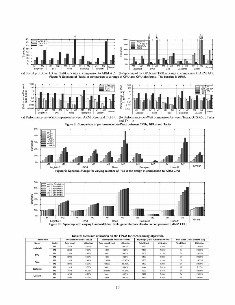
fits of our FPGA accelerators are on average in par with thedesktop-grade GTX 650 Ti GPU with the TDP of 110W. How-ever, the more high-performance Tesla K40 with the TDP of235W provides higher performance as expected. We comparethe performance-per-watt to understand the benefits of FPGAacceleration without the variations in the power budget. Figure 8acompares the performance-per-Watt for ARM A15, Xeon E3 andTABLA. Similarly, Figure 8b illustrates the performance-per-Wattfor the GPU platforms. TABLA, on average, achieves 30.1⇥ and81.7⇥ over ARM and Xeon, respectively. On the GPU side,TABLA’s FPGA accelerators provide 22.7⇥, 53.7⇥, and 30.6⇥higher performance-per-Watt compare to Tegra, GTX 650, andTesla, respectively.

Interestingly, ARM A15 achieves 2.7⇥ higher performance-per-Watt than Xeon. It is also interesting that Tesla achieves alevel of efficiency which is similar to ARM, yet it provides muchhigher performance. The TABLA-generated FPGA acceleratorsclose the performance gap to a large extent but provide muchhigher efficiency and operate at significantly lower power budget.In any case, GPUs are an attractive back-end for TABLA that canbe explored in future work. However, as Table 4 shows, theyrequire much higher power.Area and FPGA utilization. Table 6 shows the resource utiliza-tion for different components on the FPGA for each learningalgorithm. Backprop M1 utilizes the least area among all the learn-ing algorithms as it has a relatively smaller model and requiresonly 16 PEs for its default configuration. On the other hand,Reco M1 and M2 and Backprop M2 utilize a much larger areaand BRAM as their default configuration is large and they alsohave a significantly higher numbers of parameters that need tobe stored within the accelerator.7.3 Design Space ExplorationNumber of PEs per PU. During the development of the templatebased designs, we perform a design space exploration to findthe PE and PU configuration that provides the highest frequencywhile maintaining parallelism within each PU. Empirically, a PUdesign with 8 PEs strikes a balance between frequency and intra-PU parallelism. Note that this design space exploration is notthe responsibility of the programmer and is part of TABLA. It isusually done when the templates are tuned for a FPGA platformby expert hardware designers.Number of processing engines. TABLA provides a template-based architecture that can generate reconfigurable hardwareaccelerators. As described in section 6.1, the number of process-ing engines and processing units can be customized in accordancewith the algorithm. Figure 9, shows the effect of varying the num-ber of processing engines on the speedup for each benchmark.The baseline is the ARM multicore CPU. As expected, initiallythe increase in number of PEs leads to a fairly linear increase inthe speedup. However, beyond a certain number of PEs we eitherobserve diminishing returns or a decrease in the speedup. Thisobservation can be attributed to the fact that the parallelism in thealgorithms is limited and increasing the number of PEs beyond apoint would just lead to waste of resources. For example, in theLogisticR M1 benchmark, a maximum of 54 operations can bedone in parallel at a given time. Therefore, providing PEs beyond54 is inconsequential. However, our base design only allows 8PEs per PU, hence the design for LogisticR M1 has 32 PEs or 4

9

0⇥5⇥

10⇥15⇥20⇥25⇥30⇥35⇥40⇥

Spe

edup

LogisticRM1

LogisticRM2

SVMM1

SVMM2

RecoM1

RecoM2

BackpropM1

BackpropM2

LinearRM1

LinearRM2 Geomean

46⇥

ARM A15Xeon E3Tabla

M1 M2LogisticR

M1 M2Reco

M1 M2SVM

M1 M2Backprop

M1 M2LinearR Gmean

(a) Speedup of Xeon E3 and TABLA design in comparison to ARM A15.

0⇥

20⇥

40⇥

60⇥

80⇥

100⇥

Spe

edup

LogisticRM1

LogisticRM2

SVMM1

SVMM2

RecoM1

RecoM2

BackpropM1

BackpropM2

LinearRM1

LinearRM2 Geomean

433⇥

295⇥

350⇥

539⇥

Tegra K1GTX 650 TiTesla K40Tabla

M1 M2LogisticR

M1 M2Reco

M1 M2SVM

M1 M2Backprop

M1 M2LinearR

Gmean

(b) Speedup of the GPUs and TABLA design in comparison to ARM A15.Figure 7: Speedup of Tabla in comparison to a range of CPU and GPU platforms. The baseline is ARM.

0.0001

0.001

0.01

0.1

1

10

100

1000

Perfo

rman

cePe

rWat

tTO

DO

LogisticRM1

LogisticRM2

SVMM1

SVMM2

RecoM1

RecoM2

BackpropM1

BackpropM2

LinearRM1

LinearRM2 Geomean

ARM A15Xeon E3Tabla

(Log

Sca

le)

M1 M2LogisticR

M1 M2Reco

M1 M2SVM

M1 M2Backprop

M1 M2LinearR Gmean

(a) Performance-per-Watt comparison between ARM, Xeon and TABLA.

0.0001

0.001

0.01

0.1

1

10

100

1000

Perfo

rman

cePe

rWat

tTO

DO

LogisticRM1

LogisticRM2

SVMM1

SVMM2

RecoM1

RecoM2

BackpropM1

BackpropM2

LinearRM1

LinearRM2 Geomean

Tegra K1GTX 650 TiTesla K40Tabla

(Log

Sca

le)

M1 M2LogisticR

M1 M2Reco

M1 M2SVM

M1 M2Backprop

M1 M2LinearR Gmean

(b) Performance-per-Watt comparison between Tegra, GTX 650 , Teslaand TABLA

Figure 8: Comparison of performance-per-Watt between CPUs, GPUs and Tabla

0⇥

10⇥

20⇥

30⇥

40⇥

50⇥

Spe

edup

LogisticR M1 LogisticR M2 SVM M1 SVM M2 Reco M1 Reco M2 Backprop M1 Backprop M2 LinearR M1 LinearR M2 Geomean

1PE2PEs4PEs8PEs16PEs32PEs64PEs128PEs

M1 M2LogisticR

M1 M2Reco

M1 M2SVM

M1 M2Backprop

M1 M2LinearR Gmean

Figure 9: Speedup change for varying number of PEs in the design in comparison to ARM CPU

0⇥

10⇥

20⇥

30⇥

40⇥

50⇥

60⇥

Spe

edup

LogisticR M1 LogisticR M2 SVM M1 SVM M2 Reco M1 Reco M2 Backprop M1 Backprop M2 LinearR M1 LinearR M2 Geomean

0.25⇥ Bandwidth0.5⇥ Bandwidth1.0⇥ Bandwidth1.5⇥ Bandwidth2.0⇥ Bandwidth4.0⇥ Bandwidth

M1 M2LogisticR

M1 M2Reco

M1 M2SVM

M1 M2Backprop

M1 M2LinearR Gmean

Figure 10: Speedup with varying Bandwidth for Tabla generated accelerator in comparison to ARM CPU

Table 6: Resource utilization on the FPGA for each learning algorithm.

Name ModelM1M2M1M2M1M2M1M2M1M2

Benchmark

LogisticR

SVM

Reco

LinearR

Backprop

LUT (Total Available: 53200)Total Used Utilization Total Used(Bytes) Utilization

1873 3.52% 440 0.07%

3843 7.22% 1612 0.25%

1326 2.49% 440 0.07%

3296 6.20% 1612 0.25%

1326 2.49% 115504 17.90%

3296 6.20% 439652 68.15%

1916 3.60% 400 0.06%

7672 14.42% 262148 40.64%

3296 6.20% 444 0.07%

3296 6.20% 6284 0.97%

Flip-Flops (Total Available: 106400)LUT (Total Available: 53200) BRAM (Total Available: 630KB)Total Used Utilization Total Used Utilization

1230 1.16% 32 14.55%

2446 2.30% 64 29.09%

1206 1.13% 32 14.55%

2422 2.28% 64 29.09%

1206 1.13% 32 14.55%

2422 2.28% 64 29.09%

648 0.61% 16 7.27%

2602 2.45% 64 29.09%

2422 2.28% 64 29.09%

2422 2.28% 64 29.09%

Flip-Flops (Total Available: 106400) DSP Slices (Total Avilable: 220)

10

PUs. Increasing the PEs beyond 32 leads to either decrease in thespeedup or has no impact on the speedup for all the benchmarks.This anomaly is observed because as the number of PEs increasethe operational frequency also decreases due to the requirementof a wider and bigger global bus. Therefore, adding more PEsmight not improve speedup due to lack of abundant parallelismbut rather decreases the speedup due to a slower hardware. Thevarying number of PEs also gives us the optimal design thatutilizes minimum resources and still provides maximum benefitsfrom acceleration.Bandwidth sensitivity. Machine learning algorithms are bothcompute and data intensive tasks. We design the accelerator toexploit the fine-grained parallelism in the computational compo-nent of the algorithm. On the other hand, the data is providedto the compute elements of the design either through a memorybuffer in the PE or external memory. The data transferred fromexternal memory to the accelerator uses the AXI interface whichhas limited bandwidth. We do an analysis of trends observed inspeedup with this changing bandwidth between external memoryand the accelerator. Figure 10, shows the speedup for each bench-mark if the bandwidth is varied from 0.25⇥ of the default to 4⇥the default. The figure shows that bandwidth can be bottleneck atvery low values such as 0.25⇥ of the default bandwidth. As thebandwidth increases the speedup starts to increases but observediminishing returns beyond a point. By providing a bandwidththat is 4⇥ the default value the speedup numbers only increaseby 60% of the default speedup. The bandwidth sweeps are doneby creating a cycle-accurate simulator of the accelerator whichis validated against hardware.

8 Related WorkThere have been several proposed architectures that acceleratemachine learning algorithms [21, 30, 34–46]. However, TABLAfundamentally differs from these works, as it is not an accelerator.TABLA is an accelerator generator for an important class of ma-chine learning algorithms, which can be expressed as stochasticoptimization problems. Using this insight, TABLA provides ahigh-level abstraction for programmers to utilize FPGAs as theaccelerator of choice for machine learning algorithms withoutexposing the details of hardware design. There have also beenarchitectures that accelerate gradient descent [47] and conjugategradient descent [47–50]. However, these works do not specializetheir architectures in machine learning algorithms or any specificobjective function. They neither provide specialized program-ming models nor generate accelerators. Below, we discuss themost related work.Gradient descent accelerators. The work by Kesler [47] fo-cuses only on designing an accelerator suitable for differentlinear algebra operations to facilitate the gradient descent andconjugate gradient algorithms.Machine learning accelerators. There have been several suc-cessful works in the past that focus on accelerating a single ora range of fixed ML tasks. Yeh et al. and Manolakos and Sta-moulias focused on designing accelerators for a particular MLalgorithm (k-NN) [34, 35, 51]. Furthermore, work has also beendone on accelerating k-Means [36–38] and Support Vector Ma-chines (SVM) [39, 40] due to their wide applicability. Theseacceleration techniques have also been extended to conventionaland deep neural networks [21, 43–46]. However, all these accel-

erators are focused on accelerating a particular ML task.To add more flexibility and accelerate beyond one algorithm,

several works focus on designs that accelerate a range of learningalgorithms [30, 41, 42]. The work by Majumdar – MAPLE,focuses on classification and learning, while PuDianNao ac-commodates seven representative ML algorithms. Even thoughPuDianNao does cover a large spectrum of ML algorithms, itdoes not provide the flexibility to extend the accelerator for newML tasks. Besides, PuDianNao is an ASIC accelerator, whereasTABLA can generate accelerators for any platforms if properbackend support is provided.FPGA accelerators. FPGAs have gained popularity due to theirflexibility and capability to exploit copious fine-grained irregu-lar parallelism for higher performance execution. Furthermore,the work in [34, 36, 39, 40, 51–55] utilize FPGAs to acceleratea diverse set of workloads, validating the efficacy of FPGAs.LINQits [56] provides a template architecture for acceleratingdatabase queries. The work by King et. al. [57] uses Blue-spec to automatically generate a hardware-software interface forprogrammer-specified hardware-software partitions. The workby Putnam et. al. [7], designs an FPGA fabric for acceleratingranking algorithms in the Bing server. They integrate this fabricin 1632 servers at Microsoft. TABLA provides an opportunity toutilize this integrated fabric in the servers for machine learningalgorithms. Conclusively, TABLA provides a comprehensive so-lution – from programming language down to circuit design –that can generate ML accelerators.

9 ConclusionMachine learning algorithms include compute-intensive work-loads that can benefit significantly from acceleration. FPGAs arean attractive platform for accelerating these important applica-tions. However, FPGA design still requires relatively long designcycles and extensive expertise in hardware design. This paper de-scribed TABLA that aims to bridge the gap between the machinelearning algorithms and the FPGA accelerators. TABLA leveragesstochastic gradient descent as the abstraction between hardwareand software to automatically generate accelerators for a class ofstatistical machine learning algorithms. We used TABLA to gen-erate accelerators for a verity of learning algorithms targeting anoff-the-shelf FPGA platform, Xilinx Zynq. Compared to a mul-ticore Intel Xeon with vector execution, the TABLA-generatedaccelerators deliver an average speedup of 2.9⇥. Comparedto the high-performance Tesla K40 GPU accelerator, TABLAachieves 30.6⇥ higher performance-per-Watt. These gains areachieved while the programmers only write less than 50 lines ofcode. These results suggest that TABLA takes an effective stepin a widespread use of FPGAs for machine learning algorithms.We plan to make TABLA publicly available to the larger researchcommunity in order to facilitate FPGA acceleration of machinelearning algorithms.

10 AcknowledgementsThis work was supported by a Qualcomm Innovation Fellowship,NSF award CCF #1553192, Semiconductor Research Corpora-tion contract #2014-EP-2577, and a gift from Google.

11

References[1] N. Hardavellas, M. Ferdman, B. Falsafi, and A. Ailamaki.

Toward dark silicon in servers. IEEE Micro, 31(4):6–15,July–Aug. 2011.

[2] Hadi Esmaeilzadeh, Emily Blem, Renee St. Amant,Karthikeyan Sankaralingam, and Doug Burger. Darksilicon and the end of multicore scaling. In ISCA, 2011.

[3] Ganesh Venkatesh, Jack Sampson, Nathan Goulding,Saturnino Garcia, Vladyslav Bryksin, Jose Lugo-Martinez,Steven Swanson, and Michael Bedford Taylor. Conserva-tion cores: Reducing the energy of mature computations.In ASPLOS, 2010.

[4] R. H. Dennard, F. H. Gaensslen, V. L. Rideout, E. Bassous,and A. R. LeBlanc. Design of ion-implanted mosfet’swith very small physical dimensions. IEEE Journal ofSolid-State Circuits, 9, October 1974.

[5] Andrew Danowitz, Kyle Kelley, James Mao, John P. Steven-son, and Mark Horowitz. Cpu db: Recording microproces-sor history. ACM Queue, 10(4):10:10–10:27, April 2012.

[6] John Gantz and David Reinsel. Extracting value from chaos.[7] Andrew Putnam, Adrian Caulfield, Eric Chung, Derek

Chiou, Kypros Constantinides, John Demme, HadiEsmaeilzadeh, Jeremy Fowers, Gopi Prashanth, Jan Gray,Michael Haselman, Scott Hauck, Stephen Heil, AmirHormati, Joo-Young Kim, Sitaram Lanka, James R. Larus,Eric Peterson, Aaron Smith, Jason Thong, Phillip Yi Xiao,and Doug Burger. A reconfigurable fabric for acceleratinglarge-scale datacenter services. In ISCA, June 2014.

[8] Venkatraman Govindaraju, Chen-Han Ho, and KarthikeyanSankaralingam. Dynamically specialized datapaths forenergy efficient computing. In HPCA, 2011.

[9] Ganesh Venkatesh, John Sampson, Nathan Goulding,Sravanthi Kota Venkata, Steven Swanson, and MichaelTaylor. QsCores: Trading dark silicon for scalable energyefficiency with quasi-specific cores. In MICRO, 2011.

[10] Shantanu Gupta, Shuguang Feng, Amin Ansari, ScottMahlke, and David August. Bundled execution of recurringtraces for energy-efficient general purpose processing. InMICRO, 2011.

[11] Johann Hauswald, Michael A. Laurenzano, Yunqi Zhang,Cheng Li, Austin Rovinski, Arjun Khurana, Ron Dreslinski,Trevor Mudge, Vinicius Petrucci, Lingjia Tang, and JasonMars. Sirius: An open end-to-end voice and vision personalassistant and its implications for future warehouse scalecomputers. In Proceedings of the Twentieth InternationalConference on Architectural Support for ProgrammingLanguages and Operating Systems (ASPLOS), ASPLOS’15, 2015.

[12] Scott Sirowy and Alessandro Forin. Where’s the beef? whyFPGAs are so fast. Technical Report MSR-TR-2008-130,Microsoft Research, September 2008.

[13] Xilinx. Zynq-7000 all programmable soc, 2014.[14] Intel Corporation. Disrupting the data center to create the

digital services economy.[15] Stephen Boyd and Lieven Vandenberghe. Convex

optimization. Cambridge university press, 2004.[16] Xixuan Feng, Arun Kumar, Benjamin Recht, and Christo-

pher Ré. Towards a unified architecture for in-rdbms

analytics. In Proceedings of the 2012 ACM SIGMOD In-ternational Conference on Management of Data, SIGMOD’12, pages 325–336, New York, NY, USA, 2012. ACM.

[17] David C Ku and Giovanni De Micheli. High level synthesisof ASICs under timing and synchronization constraints.Kluwer Academic Publishers, 1992.

[18] Iván Cantador, Peter Brusilovsky, and Tsvi Kuflik. 2ndworkshop on information heterogeneity and fusion inrecommender systems (hetrec 2011). In Proceedings ofthe 5th ACM conference on Recommender systems, RecSys2011, New York, NY, USA, 2011. ACM.

[19] Grouplens. Movielens dataset.[20] Kamil A. Grajski. Neurocomputing, using the MasPar MP-

1. In K. W. Przytula and V. K. Prasnna, editors, Parallel Dig-ital Implementations of Neural Networks, chapter 2, pages51–76. Prentice-Hall, Englewood Cliffs, New Jersey, 1993.

[21] Hadi Esmaeilzadeh, Adrian Sampson, Luis Ceze, andDoug Burger. "neural acceleration for general-purposeapproximate programs". In MICRO, 2012.

[22] Nvidia. Jetson. http://www.nvidia.com/object/

jetson-tk1-embedded-dev-kit.html, 2015.[23] Rong-En Fan, Kai-Wei Chang, Cho-Jui Hsieh, Xiang-Rui

Wang, and Chih-Jen Lin. Liblinear: A library for largelinear classification. J. Mach. Learn. Res., 9:1871–1874,June 2008.

[24] Ryan R. Curtin, James R. Cline, Neil P. Slagle, William B.March, P. Ram, Nishant A. Mehta, and Alexander G.Gray. MLPACK: A scalable C++ machine learning library.Journal of Machine Learning Research, 14:801–805, 2013.

[25] Yangqing Jia, Evan Shelhamer, Jeff Donahue, SergeyKarayev, Jonathan Long, Ross Girshick, Sergio Guadar-rama, and Trevor Darrell. Caffe: Convolutionalarchitecture for fast feature embedding. arXiv preprintarXiv:1408.5093, 2014.

[26] Zhang Xianyi, Wang Qian, and Zhang Yunquan. Model-driven level 3 blas performance optimization on loongson3a processor. In Proceedings of the 2012 IEEE 18thInternational Conference on Parallel and DistributedSystems, ICPADS ’12, pages 684–691, Washington, DC,USA, 2012. IEEE Computer Society.

[27] Steffen Rendle. Factorization machines with libFM. ACMTrans. Intell. Syst. Technol., 3(3):57:1–57:22, May 2012.

[28] Chih-Chung Chang and Chih-Jen Lin. Libsvm: A libraryfor support vector machines. ACM Trans. Intell. Syst.Technol., 2(3):27:1–27:27, May 2011.

[29] S. Nissen. Implementation of a fast artificial neuralnetwork library (fann). Technical report, Department ofComputer Science University of Copenhagen (DIKU),2003. http://fann.sf.net.

[30] Daofu Liu, Tianshi Chen, Shaoli Liu, Jinhong Zhou,Shengyuan Zhou, Olivier Teman, Xiaobing Feng, XuehaiZhou, and Yunji Chen. Pudiannao: A polyvalent machinelearning accelerator. In Proceedings of the TwentiethInternational Conference on Architectural Support forProgramming Languages and Operating Systems, ASPLOS’15, pages 369–381, New York, NY, USA, 2015. ACM.

[31] Andreas Athanasopoulos, Anastasios Dimou, VasileiosMezaris, and Ioannis Kompatsiaris. Gpu accelerationfor support vector machines. In WIAMIS 2011: 12th

12

International Workshop on Image Analysis for MultimediaInteractive Services, Delft, The Netherlands, April 13-15,2011. TU Delft; EWI; MM; PRB, 2011.

[32] G. Teodoro, R. Sachetto, O. Sertel, M.N. Gurcan, W. Meira,U. Catalyurek, and R. Ferreira. Coordinating the use of gpuand cpu for improving performance of compute intensiveapplications. In Cluster Computing and Workshops, 2009.CLUSTER ’09. IEEE International Conference on, pages1–10, Aug 2009.

[33] Dan C. Ciresan, Ueli Meier, Jonathan Masci, Luca M.Gambardella, and Jürgen Schmidhuber. Flexible, highperformance convolutional neural networks for image classi-fication. In Proceedings of the Twenty-Second InternationalJoint Conference on Artificial Intelligence - Volume VolumeTwo, IJCAI’11, pages 1237–1242. AAAI Press, 2011.

[34] Ioannis Stamoulias and Elias S. Manolakos. Parallelarchitectures for the knn classifier – design of soft ip coresand fpga implementations. ACM Trans. Embed. Comput.Syst., 13(2):22:1–22:21, September 2013.

[35] E.S. Manolakos and I. Stamoulias. Ip-cores design forthe knn classifier. In Circuits and Systems (ISCAS),Proceedings of 2010 IEEE International Symposium on,pages 4133–4136, May 2010.

[36] H.M. Hussain, K. Benkrid, H. Seker, and A.T. Erdogan.Fpga implementation of k-means algorithm for bioinfor-matics application: An accelerated approach to clusteringmicroarray data. In Adaptive Hardware and Systems (AHS),2011 NASA/ESA Conference on, pages 248–255, June 2011.

[37] Tsutomu Maruyama. Real-time k-means clustering forcolor images on reconfigurable hardware. In Proceedings ofthe 18th International Conference on Pattern Recognition- Volume 02, ICPR ’06, pages 816–819, Washington, DC,USA, 2006. IEEE Computer Society.

[38] A.Gda.S. Filho, A.C. Frery, C.C. de Araujo, H. Alice,J. Cerqueira, J.A. Loureiro, M.E. de Lima, Mdas.G.S.Oliveira, and M.M. Horta. Hyperspectral images clusteringon reconfigurable hardware using the k-means algorithm. InIntegrated Circuits and Systems Design, 2003. SBCCI 2003.Proceedings. 16th Symposium on, pages 99–104, Sept 2003.

[39] M. Papadonikolakis and C. Bouganis. A heterogeneousfpga architecture for support vector machine training.In Field-Programmable Custom Computing Machines(FCCM), 2010 18th IEEE Annual International Symposiumon, pages 211–214, May 2010.

[40] S. Cadambi, I. Durdanovic, V. Jakkula, M. Sankaradass,E. Cosatto, S. Chakradhar, and H.P. Graf. A massivelyparallel fpga-based coprocessor for support vectormachines. In Field Programmable Custom ComputingMachines, 2009. FCCM ’09. 17th IEEE Symposium on,pages 115–122, April 2009.

[41] A. Majumdar, S. Cadambi, and S.T. Chakradhar. Anenergy-efficient heterogeneous system for embeddedlearning and classification. Embedded Systems Letters,IEEE, 3(1):42–45, March 2011.

[42] Abhinandan Majumdar, Srihari Cadambi, Michela Becchi,Srimat T. Chakradhar, and Hans Peter Graf. A massivelyparallel, energy efficient programmable accelerator forlearning and classification. ACM Trans. Archit. CodeOptim., 9(1):6:1–6:30, March 2012.

[43] C. Farabet, B. Martini, B. Corda, P. Akselrod, E. Culurciello,and Y. LeCun. Neuflow: A runtime reconfigurable dataflowprocessor for vision. In Computer Vision and PatternRecognition Workshops (CVPRW), 2011 IEEE ComputerSociety Conference on, pages 109–116, June 2011.

[44] Tianshi Chen, Zidong Du, Ninghui Sun, Jia Wang,Chengyong Wu, Yunji Chen, and Olivier Temam. Diannao:a small-footprint high-throughput accelerator for ubiquitousmachine-learning. In Proceedings of the 19th internationalconference on Architectural support for programminglanguages and operating systems, pages 269–284, 2014.

[45] A.A. Maashri, M. DeBole, M. Cotter, N. Chandramoorthy,Yang Xiao, V. Narayanan, and C. Chakrabarti. Accel-erating neuromorphic vision algorithms for recognition.In Design Automation Conference (DAC), 2012 49thACM/EDAC/IEEE, pages 579–584, June 2012.

[46] Thierry Moreau, Mark Wyse, Jacob Nelson, AdrianSampson, Hadi Esmaeilzadeh, Luis Ceze, and Mark Oskin.SNNAP: Approximate computing on programmable socsvia neural acceleration. In HPCA, 2015.

[47] D. Kesler, B. Deka, and R. Kumar. A hardware accelerationtechnique for gradient descent and conjugate gradient. InApplication Specific Processors (SASP), 2011 IEEE 9thSymposium on, pages 94–101, June 2011.

[48] Antonio Roldao and George A. Constantinides. Ahigh throughput fpga-based floating point conjugategradient implementation for dense matrices. ACM Trans.Reconfigurable Technol. Syst., 3(1):1:1–1:19, January 2010.

[49] G.R. Morris, V.K. Prasanna, and R.D. Anderson. Ahybrid approach for mapping conjugate gradient ontoan fpga-augmented reconfigurable supercomputer. InField-Programmable Custom Computing Machines, 2006.FCCM ’06. 14th Annual IEEE Symposium on, pages 3–12,April 2006.

[50] D. DuBois, A. DuBois, T. Boorman, C. Connor, andS. Poole. An implementation of the conjugate gradientalgorithm on fpgas. In Field-Programmable CustomComputing Machines, 2008. FCCM ’08. 16th InternationalSymposium on, pages 296–297, April 2008.

[51] Yao-Jung Yeh, Hui-Ya Li, Wen-Jyi Hwang, and Chiung-Yao Fang. Fpga implementation of knn classifier basedon wavelet transform and partial distance search. InProceedings of the 15th Scandinavian Conference on ImageAnalysis, SCIA’07, pages 512–521, Berlin, Heidelberg,2007. Springer-Verlag.

[52] Andrew R. Putnam, Dave Bennett, Eric Dellinger, JeffMason, and Prasanna Sundararajan. CHiMPS: A high-levelcompilation flow for hybrid CPU-FPGA architectures. InFPGA, 2008.

[53] Yi Shan, Bo Wang, Jing Yan, Yu Wang, Ningyi Xu, andHuazhong Yang. Fpmr: Mapreduce framework on fpga. InProceedings of the 18th Annual ACM/SIGDA InternationalSymposium on Field Programmable Gate Arrays, FPGA’10, pages 93–102, New York, NY, USA, 2010. ACM.

[54] Jeremy Fowers, Kalin Ovtcharov, Karin Strauss, EricChung, and Greg Stitt. A high memory bandwidth fpgaaccelerator for sparse matrix-vector multiplication. InInternational Symposium on Field-Programmable CustomComputing Machines. IEEE, May 2014.

13

[55] Eric S. Chung, James C. Hoe, and Ken Mai. Coram: Anin-fabric memory architecture for fpga-based computing.In Proceedings of the 19th ACM/SIGDA InternationalSymposium on Field Programmable Gate Arrays, FPGA’11, pages 97–106, New York, NY, USA, 2011. ACM.

[56] Eric S. Chung, John D. Davis, and Jaewon Lee. Linqits:Big data on little clients. In Proceedings of the 40th AnnualInternational Symposium on Computer Architecture, ISCA’13, pages 261–272, New York, NY, USA, 2013. ACM.

[57] M. King, A. Khan, A. Agarwal, O. Arcas, and Arvind. Gen-erating infrastructure for fpga-accelerated applications. InField Programmable Logic and Applications (FPL), 201323rd International Conference on, pages 1–6, Sept 2013.

14