DTMRI Segmentation using DT-Snakes and DT-Livewire

Ghassan Hamarneh and Judith HradskyMedical Image Analysis Lab, School of Computing Science, Simon Fraser University

Burnaby, BC, V5A 1S6, Canada

Abstract— In this paper we extend two popular classicalscalar medical image segmentation techniques to diffusion tensormagnetic resonance images (DTMRI). We propose DT-snakesand DT-livewire through modifying the external image forcesin snakes and cost terms in livewire. The new forces and costterms are derived from and operate on a DT field ratherthan a scalar image. This is achieved by making use of recentadvances in DT calculus and DT dissimilarity measures, as wellas DT smoothing and DT interpolation. Proper quantification oftensor dissimilarity allows for defining spatial gradient vectorsand gradient magnitudes of DT fields, an essential componentfor attracting snakes or livewire to target boundaries in DTimages. DT calculus enables weighted averaging of tensors whichis essential for both pre-smoothing of DT images prior tosegmentation, as well as interpolation of tensors on non-gridpositions in the image. We evaluate different recent DT tensordissimilarity metrics including the Log-Euclidean and the squareroot of the J-divergence. We present qualitative and quantitativeDT segmentation results on both synthetic and real cardiac andbrain DTMRI data.

I. INTRODUCTION

Diffusion is the process by which molecules are transportedfrom one part of a medium to another. The flux of diffusingmolecules is a result of their random Brownian motion inconcentration gradients and is described by Fick’s law. Diffu-sion tensor magnetic resonance imaging (DTMRI) records thediffusion characteristics of water molecules along fiber tractsin-vivo and is becoming increasingly valuable for assessingthe effects of disease progression and treatment evaluation onfiber connectivity and diffusion properties [1], [2]. In DTMRI,typically each voxel of the 3D image is assigned a rank three,second order diffusion tensor forming a 3D tensor field. Eachtensor is expressed as a 3×3 symmetric, positive semi-definite(PSD) matrix (with nonnegative eigenvalues). The generalclasses of medical image analysis algorithms performed onscalar medical images (filtering, segmentation, registration andvisualization of X-ray CT, T1-weighted MRI, ultrasound, andothers) need to be extended to DTMRI tensor fields in orderto glean quantitative and qualitative information, potentiallyimproving computer aided diagnosis, follow up of treatmentand disease progression, and statistical analysis of structuraland functional variability. In the following paragraphs wereview important contributions in processing, segmentation,and registration of tensor field data.

The primary goal of processing is to reduce the noise in theDTMRI data that occurs due to various imaging acquisitionartifacts. There exist numerous techniques for image process-ing of scalar fields; an essential task in any image processingpipelines. However, only a few methods have been recentlyextended to perform basic processing and reduce noise in

diffusion tensor image data, for example median filtering,morphological operations, interpolation, and anisotropic edgepreserving smoothing [3], [4], [5], [6].

Identifying and delineating regions of interest (ROI) inimage data is necessary for performing subsequent quantitativeanalysis and qualitative visualization. Segmentation methodsrely on (a) identifying nearby voxels with similar diffusionproperties and grouping them into one coherent structure, (b)identifying edges in the DTMRI and linking them to formseparating boundaries between neighboring structures, and (c)incorporating prior knowledge about the shape characteristicsof the different target structures to segment. These intuitiveideas are very well understood for the scalar case, but haveonly recently been the focus of research for tensor fields [7],[8], [9], [10], [11], [12], [13], [14], [15], [16].

To facilitate viewing and interrogating DTMRI segmen-tation and visualization results within the context of othermedical imaging modalities (e.g. structural MRI), the data setsmust be properly fused by bringing them into proper spatialalignment. Image registration is also needed for quantitativeand qualitative longitudinal analysis tasks, in which DTMRIdata of the same subject at different times must be compared[17], [18], [19], [20].

In this paper we focus on extending two classical andpopular scalar image segmentation techniques allowing usto delineate anatomical regions and boundaries directly fromDTMRI fields. We utilize the full information in the tensorswithout being forced to operate on a single derived scalarimage such as apparent diffusion coefficient (ADC) or relativeanisotropy (RA) [2].

Specifically, we extend snakes [21] and livewires [22] to DT-snakes and DT-livewire primarily by redefining the externalimage forces and cost terms in snakes and livewire, respec-tively. The new forces and cost terms now operate directly inthe DT field rather than scalar images. This extension relieson recent definitions of tensor dissimilarity metrics, weightedtensor averaging, smoothing and interpolation of DT fields[8], [23], [24]. Since the snakes and livewire methods areformulated such that their contours are attracted to boundaries,the definition of target boundaries is revisited for DTMRI datamaking use of tensor dissimilarity measures to calculate tensorgradients. We evaluate different alternative DT dissimilaritymetrics including the Log-Euclidean and the square root ofthe J-divergence [23], [8]. Further, because it is known thatgradient calculation is sensitive to noise, and in order toavoid having contours attracted to noisy data, the image datais pre-smoothed prior to segmentation, utilizing a DT edge-preserving smoothing algorithm (bilateral DT filtering) [24].

2006 IEEE International Symposium on Signal Processing and Information Technology

0-7803-9754-1/06/$20.00©2006 IEEE 513

Furthermore, to continue to have deformable models withsubpixel accuracy, tensor values need to be evaluated at non-grid positions requiring specialized DT interpolation methods.

The remainder of the paper is organized as follows. In sec-tion II we summarize alternative ways of quantifying diffusiontensor dissimilarity and how it is used for tensor gradientcalculation. We follow with a summary of the approach weadopt for tensor smoothing and interpolation, and then utilizethe previous concepts to propose the extension of snakes andlivewire to operate on DT data directly without the need toextract scalar features. In section III we present qualitativeexperimental and quantitative validation results on syntheticand real brain and cardiac DTMRI data. We summarize anddraw conclusions in section IV.

II. METHODS

A. Diffusion Tensor Dissimilarity and Gradient Estimation

Tensors in DTMRI are 3×3 PSD matrices that do not form avector space thus requiring special attention when performingDT calculations [25]. To perform segmentation we need a wayto measure differences between tensors as this will allow usto define gradient vectors that are essential for DT-snakesand DT-livewire, and other potential boundary based DTsegmentation techniques. Ideally, tensor dissimilarity shouldreflect the geodesic distance on the space of allowable tensors;a convex half-cone [26], [25]. Therefore, choosing Euclidean‖T1 − T2‖, or Frobenius norm ‖T1 − T2‖F , where ‖A‖F =√

Tr(AAH) and Tr(...) denotes trace, is not appropriate formeasuring distances between tensors T1 and T2. The followingare the two main alternatives tensor distance measures recentlyintroduced in the literature which we will utilize to define DTgradients. The Log-Euclidean distance and the affine-invariantsquare root of the J-divergence [8], denoted respectively asdTLE

and dTJ, are given by

dTLE(T1, T2) = ‖log(T1) − log(T2)‖ (1)

dTJ(T1, T2) =

12

√Tr(T−1

1 T2 + T−12 T1) − 2n (2)

where log denotes matrix logarithm, and n = 3 for threedimensional diffusion.

The tensor field gradient can now be defined in a manneranalogous to central finite difference approximation of thescalar 2D image gradient ∇f(x, y),

∇f(x, y) =12

[f(x + 1, y) − f(x − 1, y)f(x, y + 1) − f(x, y − 1)

]. (3)

We replace the finite difference (subtraction) approximationwith central tensor dissimilarity to obtain the tensor gradientvector ∇T at any location (x, y) as follows,

∇T (x, y) =12

[dT ((T (x + 1, y), T (x − 1, y)))dT ((T (x, y + 1), T (x, y − 1)))

](4)

where dT is either one of the tensor distance measurespresented earlier (equation (1) or (2)).

B. Diffusion Tensor Smoothing

To produce stable gradient calculation and to avoid havingcontours attracted to noisy data, the image data is typically pre-smoothed prior to segmentation. We utilize a recently proposedbilateral edge-preserving DT field smoothing [24] that relieson calculating a weighted average of tensors using

T (x) = k(x)−1exp

(N∑

i=1

wi(x)log(T (ξi))

)(5)

k(x) =N∑

i=1

wi(x) (6)

where exp is the matrix logarithm, T (x) is the tensor resultingfrom a weighted averaging of N tensors, T (ξi), in the neigh-bourhood of x. The corresponding weights, wi, are defined tobe inversely proportional to the spatial distance and the tensordissimilarity between the neighboring tensors and the centertensor, as follows

wi(x) = αf1(dT (T (x), T (ξi))) + (1 − α)f2(dS(x, ξi)) (7)

where α ∈ [0, 1] controls the relative emphasis on spatialversus tensor distance, dT (T (x), T (ξi)) and dS(x, ξi) arethe tensor dissimilarity and spatial distance between T (x)and T (ξi), respectively, and f1 and f2 are monotonicallydecreasing functions that map the range of tensor-dissimilarityvalues and spatial distances, respectively, to the interval [0, 1].

C. Diffusion Tensor Interpolation

To extend the classical deformable models with subpixelaccuracy, tensor values need to be evaluated at non-gridpositions, requiring specialized DT interpolation methods. Asdescribed in [24], DT field interpolation is treated as a specialcase of (5). A tensor is interpolated at any non-grid positionusing the Log-Euclidean weighted sum of N nearby tensors,T (ξ), where the weights are inversely proportional to thespatial distance between the non-grid position x and thelocations of the nearby tensors, ξ. This is intuitively andconveniently obtained by setting α = 0 in equation (??).

Based on the ideas put forward thus far, in the following sec-tions we extend two classical segmentation methods, namelysnakes and livewire [21], [22], to operate on diffusion tensordata.

D. DT-Snakes for DTMRI

Snakes are energy-minimizing parametric contours that de-form to segment target structures. We extend snakes to operateon DTMRI data. Our implementation takes the form of apolygonal discrete active contour model [21], where the nodes(vertices) of the snake are updated through the application ofinternal (tensile and flexural) and external (image and inflation)forces. Internal forces are implemented as in the scalar imagecase [27], while external forces are modified to operate onDT fields in the following ways. The image force, F image

i ,at snake node i, attracts the snake to DT field edges and isredefined as follows (Fig. 1)

F imagei = −∇‖∇T (xi, yi)‖ (8)

514

(a) (b)

(c) (d)

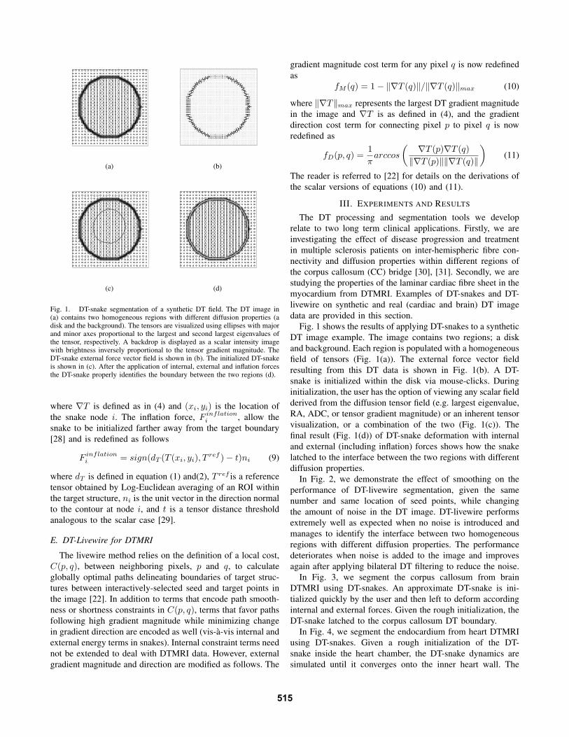
Fig. 1. DT-snake segmentation of a synthetic DT field. The DT image in(a) contains two homogeneous regions with different diffusion properties (adisk and the background). The tensors are visualized using ellipses with majorand minor axes proportional to the largest and second largest eigenvalues ofthe tensor, respectively. A backdrop is displayed as a scalar intensity imagewith brightness inversely proportional to the tensor gradient magnitude. TheDT-snake external force vector field is shown in (b). The initialized DT-snakeis shown in (c). After the application of internal, external and inflation forcesthe DT-snake properly identifies the boundary between the two regions (d).

where ∇T is defined as in (4) and (xi, yi) is the location ofthe snake node i. The inflation force, F inflation

i , allow thesnake to be initialized farther away from the target boundary[28] and is redefined as follows

F inflationi = sign(dT (T (xi, yi), T ref ) − t)ni (9)

where dT is defined in equation (1) and(2), T ref is a referencetensor obtained by Log-Euclidean averaging of an ROI withinthe target structure, ni is the unit vector in the direction normalto the contour at node i, and t is a tensor distance thresholdanalogous to the scalar case [29].

E. DT-Livewire for DTMRI

The livewire method relies on the definition of a local cost,C(p, q), between neighboring pixels, p and q, to calculateglobally optimal paths delineating boundaries of target struc-tures between interactively-selected seed and target points inthe image [22]. In addition to terms that encode path smooth-ness or shortness constraints in C(p, q), terms that favor pathsfollowing high gradient magnitude while minimizing changein gradient direction are encoded as well (vis-a-vis internal andexternal energy terms in snakes). Internal constraint terms neednot be extended to deal with DTMRI data. However, externalgradient magnitude and direction are modified as follows. The

gradient magnitude cost term for any pixel q is now redefinedas

fM (q) = 1 − ‖∇T (q)‖/‖∇T (q)‖max (10)

where ‖∇T‖max represents the largest DT gradient magnitudein the image and ∇T is as defined in (4), and the gradientdirection cost term for connecting pixel p to pixel q is nowredefined as

fD(p, q) =1π

arccos

( ∇T (p)∇T (q)‖∇T (p)‖‖∇T (q)‖

)(11)

The reader is referred to [22] for details on the derivations ofthe scalar versions of equations (10) and (11).

III. EXPERIMENTS AND RESULTS

The DT processing and segmentation tools we developrelate to two long term clinical applications. Firstly, we areinvestigating the effect of disease progression and treatmentin multiple sclerosis patients on inter-hemispheric fibre con-nectivity and diffusion properties within different regions ofthe corpus callosum (CC) bridge [30], [31]. Secondly, we arestudying the properties of the laminar cardiac fibre sheet in themyocardium from DTMRI. Examples of DT-snakes and DT-livewire on synthetic and real (cardiac and brain) DT imagedata are provided in this section.

Fig. 1 shows the results of applying DT-snakes to a syntheticDT image example. The image contains two regions; a diskand background. Each region is populated with a homogeneousfield of tensors (Fig. 1(a)). The external force vector fieldresulting from this DT data is shown in Fig. 1(b). A DT-snake is initialized within the disk via mouse-clicks. Duringinitialization, the user has the option of viewing any scalar fieldderived from the diffusion tensor field (e.g. largest eigenvalue,RA, ADC, or tensor gradient magnitude) or an inherent tensorvisualization, or a combination of the two (Fig. 1(c)). Thefinal result (Fig. 1(d)) of DT-snake deformation with internaland external (including inflation) forces shows how the snakelatched to the interface between the two regions with differentdiffusion properties.

In Fig. 2, we demonstrate the effect of smoothing on theperformance of DT-livewire segmentation, given the samenumber and same location of seed points, while changingthe amount of noise in the DT image. DT-livewire performsextremely well as expected when no noise is introduced andmanages to identify the interface between two homogeneousregions with different diffusion properties. The performancedeteriorates when noise is added to the image and improvesagain after applying bilateral DT filtering to reduce the noise.

In Fig. 3, we segment the corpus callosum from brainDTMRI using DT-snakes. An approximate DT-snake is ini-tialized quickly by the user and then left to deform accordinginternal and external forces. Given the rough initialization, theDT-snake latched to the corpus callosum DT boundary.

In Fig. 4, we segment the endocardium from heart DTMRIusing DT-snakes. Given a rough initialization of the DT-snake inside the heart chamber, the DT-snake dynamics aresimulated until it converges onto the inner heart wall. The

515

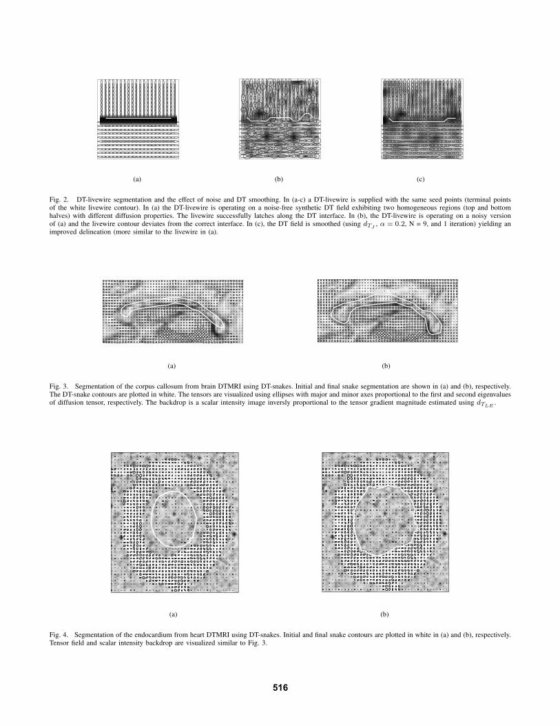
(a) (b) (c)

Fig. 2. DT-livewire segmentation and the effect of noise and DT smoothing. In (a-c) a DT-livewire is supplied with the same seed points (terminal pointsof the white livewire contour). In (a) the DT-livewire is operating on a noise-free synthetic DT field exhibiting two homogeneous regions (top and bottomhalves) with different diffusion properties. The livewire successfully latches along the DT interface. In (b), the DT-livewire is operating on a noisy versionof (a) and the livewire contour deviates from the correct interface. In (c), the DT field is smoothed (using dTJ

, α = 0.2, N = 9, and 1 iteration) yielding animproved delineation (more similar to the livewire in (a).

(a) (b)

Fig. 3. Segmentation of the corpus callosum from brain DTMRI using DT-snakes. Initial and final snake segmentation are shown in (a) and (b), respectively.The DT-snake contours are plotted in white. The tensors are visualized using ellipses with major and minor axes proportional to the first and second eigenvaluesof diffusion tensor, respectively. The backdrop is a scalar intensity image inversly proportional to the tensor gradient magnitude estimated using dTLE

.

(a) (b)

Fig. 4. Segmentation of the endocardium from heart DTMRI using DT-snakes. Initial and final snake contours are plotted in white in (a) and (b), respectively.Tensor field and scalar intensity backdrop are visualized similar to Fig. 3.

516

(a) (b)

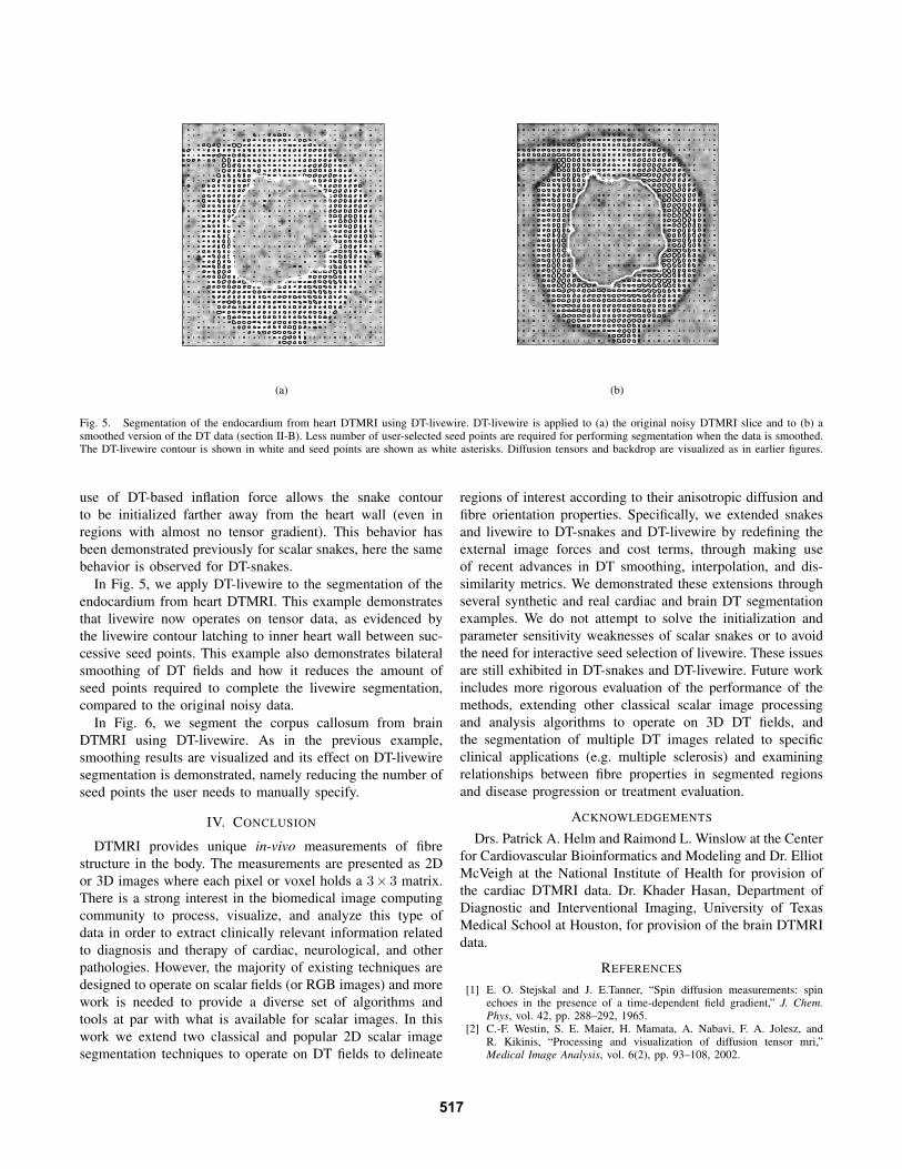
Fig. 5. Segmentation of the endocardium from heart DTMRI using DT-livewire. DT-livewire is applied to (a) the original noisy DTMRI slice and to (b) asmoothed version of the DT data (section II-B). Less number of user-selected seed points are required for performing segmentation when the data is smoothed.The DT-livewire contour is shown in white and seed points are shown as white asterisks. Diffusion tensors and backdrop are visualized as in earlier figures.

use of DT-based inflation force allows the snake contourto be initialized farther away from the heart wall (even inregions with almost no tensor gradient). This behavior hasbeen demonstrated previously for scalar snakes, here the samebehavior is observed for DT-snakes.

In Fig. 5, we apply DT-livewire to the segmentation of theendocardium from heart DTMRI. This example demonstratesthat livewire now operates on tensor data, as evidenced bythe livewire contour latching to inner heart wall between suc-cessive seed points. This example also demonstrates bilateralsmoothing of DT fields and how it reduces the amount ofseed points required to complete the livewire segmentation,compared to the original noisy data.

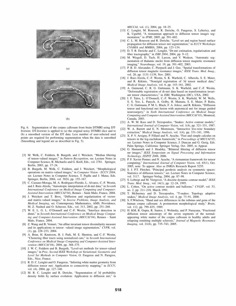
In Fig. 6, we segment the corpus callosum from brainDTMRI using DT-livewire. As in the previous example,smoothing results are visualized and its effect on DT-livewiresegmentation is demonstrated, namely reducing the number ofseed points the user needs to manually specify.

IV. CONCLUSION

DTMRI provides unique in-vivo measurements of fibrestructure in the body. The measurements are presented as 2Dor 3D images where each pixel or voxel holds a 3× 3 matrix.There is a strong interest in the biomedical image computingcommunity to process, visualize, and analyze this type ofdata in order to extract clinically relevant information relatedto diagnosis and therapy of cardiac, neurological, and otherpathologies. However, the majority of existing techniques aredesigned to operate on scalar fields (or RGB images) and morework is needed to provide a diverse set of algorithms andtools at par with what is available for scalar images. In thiswork we extend two classical and popular 2D scalar imagesegmentation techniques to operate on DT fields to delineate

regions of interest according to their anisotropic diffusion andfibre orientation properties. Specifically, we extended snakesand livewire to DT-snakes and DT-livewire by redefining theexternal image forces and cost terms, through making useof recent advances in DT smoothing, interpolation, and dis-similarity metrics. We demonstrated these extensions throughseveral synthetic and real cardiac and brain DT segmentationexamples. We do not attempt to solve the initialization andparameter sensitivity weaknesses of scalar snakes or to avoidthe need for interactive seed selection of livewire. These issuesare still exhibited in DT-snakes and DT-livewire. Future workincludes more rigorous evaluation of the performance of themethods, extending other classical scalar image processingand analysis algorithms to operate on 3D DT fields, andthe segmentation of multiple DT images related to specificclinical applications (e.g. multiple sclerosis) and examiningrelationships between fibre properties in segmented regionsand disease progression or treatment evaluation.

ACKNOWLEDGEMENTS

Drs. Patrick A. Helm and Raimond L. Winslow at the Centerfor Cardiovascular Bioinformatics and Modeling and Dr. ElliotMcVeigh at the National Institute of Health for provision ofthe cardiac DTMRI data. Dr. Khader Hasan, Department ofDiagnostic and Interventional Imaging, University of TexasMedical School at Houston, for provision of the brain DTMRIdata.

REFERENCES

[1] E. O. Stejskal and J. E.Tanner, “Spin diffusion measurements: spinechoes in the presence of a time-dependent field gradient,” J. Chem.Phys, vol. 42, pp. 288–292, 1965.

[2] C.-F. Westin, S. E. Maier, H. Mamata, A. Nabavi, F. A. Jolesz, andR. Kikinis, “Processing and visualization of diffusion tensor mri,”Medical Image Analysis, vol. 6(2), pp. 93–108, 2002.

517

(a)

(b)

Fig. 6. Segmentation of the corpus callosum from brain DTMRI using DT-livewire. DT-livewire is applied to (a) the original noisy DTMRI slice and to(b) a smoothed version of the DT data. Less number of user-selected seedpoints are required for performing segmentation when the data is smoothed(Smoothing and legend are as described in Fig. 5).

[3] M. Welk, C. Feddern, B. Burgeth, and J. Weickert, “Median filteringof tensor-valued images,” in Pattern Recognition, ser. Lecture Notes inComputer Science, B. Michaelis and G. Krell, Eds., vol. 2781. Springer,Berlin, 2003, pp. 17–24.

[4] B. Burgeth, M. Welk, C. Feddern, and J. Weickert, “Morphologicaloperations on matrix-valued images,” in Computer Vision - ECCV 2004,ser. Lecture Notes in Computer Science, T. Pajdla and J. Matas, Eds.Springer, Berlin, 2004, vol. 3024, pp. 155–167.

[5] C. Castano-Moraga, M. A. Rodrigues-Florido, L. Alvarez, C.-F. Westin,and J. Ruiz-Alzola, “Anisotropic interpolation of dt-mri data,” in SeventhInternational Conference on Medical Image Computing and Computer-Assisted Intervention (MICCAI’04), Rennes - Saint Malo, France, 2004.

[6] J. Weickert and T. Brox, “Diffusion and regularization of vector-and matrix-valued images,” in Inverse Problems, Image Analysis, andMedical Imaging, ser. Contemporary Mathematics, AMS, Providence,M. Z. Nashed and O. Scherzer, Eds., vol. 313, 2002, pp. 251–268.

[7] W. E. L. G. L. O’Donnell and C.-F. Westin, “Interface detection indtmri,” in Seventh International Conference on Medical Image Comput-ing and Computer-Assisted Intervention (MICCAI’04), Rennes - SaintMalo, France, 2004.

[8] Z. Wang and B. Vemuri, “An affine invariant tensor dissimilarity measureand its applications to tensor- valued image segmentation,” CVPR, vol.(1), pp. 228–233, 2004.

[9] A. Brun, H. Knutsson, H. J. Park, M. E. Shenton, and C.-F. Westin,“Clustering fiber tracts using normalized cuts,” in Seventh InternationalConference on Medical Image Computing and Computer-Assisted Inter-vention (MICCAI’04), 2004, pp. 368–375.

[10] J. W. C. Feddern and B. Burgeth, “Level-set methods for tensor-valuedimages,” in Proc. Second IEEE Workshop on Variational, Geometric andLevel Set Methods in Computer Vision, O. Faugeras and N. Paragios,Eds., Nice, France.

[11] R. D. C. Lenglet and O. Faugeras, “Inferring white matter geometry fromdiffusion tensor mri: Application to connectivity mapping,” in ECCV,vol. (4), 2004, pp. 127–140.

[12] M. R. C. Lenglet and R. Deriche, “Segmentation of 3d probabilitydensity fields by surface evolution: Application to diffusion mri,” in

MICCAI, vol. (1), 2004, pp. 18–25.[13] C. Lenglet, M. Rousson, R. Deriche, O. Faugeras, S. Lehericy, and

K. Ugurbil, “A riemannian approach to diffusion tensor images seg-mentation,” in IPMI, 2005, pp. 591–602.

[14] C. L. M. Rousson and R. Deriche, “Level set and region based surfacepropagation for diffusion tensor mri segmentation,” in ECCV WorkshopsCVAMIA and MMBIA, 2004, pp. 123–134.

[15] D. T. R. Deriche and C. Lenglet, “Dt-mri estimation, regularization andfiber tractography,” in ISBI 2004, 2004, pp. 9–12.

[16] M. Wiegell, D. Tuch, H. Larson, and V. Wedeen, “Automatic seg-mentation of thalamic nuclei from diffusion tensor magnetic resonanceimaging,” NeuroImage, vol. 19, pp. 391–402, 2003.

[17] P. B. D. Alexander, C. Pierpaoli and J. Gee, “Spatial transformations ofdiffusion tensor magnetic resonance images,” IEEE Trans. Med. Imag.,vol. 20, pp. 1131–1139, Nov. 2001.

[18] J. Ruiz-Alzola, C.-F. Westin, S. K. Warfield, C. Alberola, S. E. Maier,and R. Kikinis, “Nonrigid registration of 3d tensor medical data,”Medical Image Analysis, vol. 6, pp. 143–161, 2002.

[19] A. Guimond, C. R. G. Guttmann, S. K. Warfield, and C.-F. Westin,“Deformable registration of dt-mri data based on transformation invari-ant tensor characteristics,” in ISBI, Washington (DC), USA, 2002.

[20] I. F. Talos, L. O’Donnell, C.-F. Westin, S. K. Warfield, W. M. Wells,S. S. Yoo, L. Panych, A. Golby, H. Mamata, S. E. Maier, P. Ratiu,C. G. Guttmann, P. M. L. Black, F. A. Jolesz, and R. Kikinis, “Diffusiontensor and functional mri fusion with anatomical mri for image guidedneurosurgery,” in Sixth International Conference on Medical ImageComputing and Computer-Assisted Intervention (MICCAI’03), Montreal,Canada, 2003.

[21] A. W. M. Kass and D. Terzopoulos, “Snakes: Active contour models,”International Journal of Computer Vision, vol. 1(4), pp. 321–331, 1987.

[22] W. A. Barrett and E. N. Mortensen, “Interactive live-wire boundaryextraction,” Medical Image Analysis, vol. 1(4), pp. 331–341, 1996.

[23] X. P. V. Arsigny, P. Fillard and N. Ayache, “Fast and simple calculus ontensors in the log-euclidean framework,” in Proceedings of MICCAI’05,ser. Lecture Notes in Computer Science, J. Duncan and G. Gerig, Eds.Palm Springs, California: Springer Verlag, Oct. 2005, to Appear.

[24] G. Hamarneh and J. Hradsky, “Bilateral filtering of diffusion tensormr images,” IEEE Symposium on Signal Processing and InformationTechnology, ISSPIT 2006, 2006.

[25] P. F. Xavier Pennec and N. Ayache, “A riemannian framework for tensorcomputing,” International Journal of Computer Vision, vol. 65(1), Oct.2005, note: To appear. Also as INRIA Research Report 5255.

[26] S. J. P.T. Fletcher, “Principal geodesic analysis on symmetric spaces:Statistics of diffusion tensors,” ser. Lecture Notes in Computer Science,vol. 3117. Springer-Verlag, 2004, pp. 87–98.

[27] S. Lobregt and M. Viergever, “A discrete dynamic contour model,” IEEETrans. Med. Imag., vol. 14(1), pp. 12–24, 1995.

[28] L. Cohen, “On active contour models and balloons,” CVGIP, vol. 53,no. 2, pp. 211–218, March 1991.

[29] T. McInerney and D. Terzopoulos, “T-snakes: Topology adaptivesnakes,” Medical Image Analysis, vol. 4, pp. 73–91, 2000.

[30] S. F.Witelson, “Hand and sex differences in the isthmus and genu of thehuman corpus callosum: A postmortem morphological study,” Brain,vol. 112, pp. 799–835, 1989.

[31] H. KM, R. Gupta, R. Santos, J. Wolinsky, and P. Narayana, “Fractionaldiffusion tensor anisotropy of the seven segments of the normal-appearing white matter of the corpus callosum in healthy adults andrelapsing remitting multiple sclerosis,” Journal of Magnetic ResonanceImaging, vol. 21(6), pp. 735–743, 2005.

518