Embed Size (px)
Citation preview
An Empirical Potential for Hydrogen Bond Energies
Determination of the Orientation of Anthracene Molecules in the Unit Cell by means of a
Refractivity Method
Some Ab Initio Calculations Involving Acetonitrile Exchange Reaction
by
Szu-Lin Chen
Dissertation submitted to the Faculty of the
Virginia Polytechnic Institute and State University
in partial fulfillment of the requirements for the degree of
Doctor of Philosophy
John C. Schug-
Brian E. Hanson
in
Chemistry
APPROVED:
Jifilmy 't Viers, Chairman
May, 1987
Blacksburg, Virginia
James P. W~tm~
Gerald V. Gibbs
An Empirical Potential for Hydrogen Bond Energies
Determination of the Orientation of Anthracene Molecules in the Unit Cell by means of a
Refractivity Method
Topic I
Some Ab Initio Calculations Involving Acet.onitrile Exchange Reaction
by
Szu-Lin Chen
Jimmy W. Viers, Chairman
Chemistry
(ABSTRACT)
An empirical potential for calculating hydrogen bonding energies is developed for systems of the
type A-H--B, where A and/or Bis oxygen or nitrogen. Point charge and van der Waals interaction
are included in the potential. The parameters of the potential were optimized by means of a
simplex algorithm within a range of A-B distances from 2.8 A through 5.0 A. The root mean
square deviation between the empirical potential and the ab initio results of 216 configurations of
(H20)i, (NH3)i and Nlh•I-IzO is 0.9 kcal/mol and 0.5 kcal/mol for 61 configurations of methanol
dimers. Applications of the potential to water dimers, ammonia dimers, their mixed dimers, water
oligomers and ice-h as well as the P form of the methanol crystal show that the potential yields
reasonable results compared to those computed by "ab initio" methods using 6-31G* basis sets.
The potential is compatible with MM2 program. It is simpler than earlier potentials in that neither
dipoles nor Morse potentials are involved. It should be superior to the empirical potentials devel-
oped by Jorgensen that used ST0-3G ab initio calculated results as the standards. The potential
might be useful for estimation of hydrogen bond energies in a local part of a large molecule to avoid
the prohibitive expense of ab initio calculation.

Topic II
The monoclinic anthracene crystal is used as an example to demonstrate the feasibility of opti-
mizing the orientation of molecules in the unit cell by matching calculated and experimental
refractivity ellipsoids using a simplex algorithm. The calculated refractivity ellipsoid is detennU:ted
by use of an empirical formula using bond directional polarizabilities. Optimization of the molec-
ular orientations to provide the best fit to the experimental ellipsoid starting from several assumed
orientations results in fits for which the maximum deviation from the experimental molecular ori-
entation was no more than 10 degrees. The method can be applied to other monoclinic molecular
crystals directly and could be extended to other crystal systems with anisotropic optical properties.
Topic III
Three mechanisms (Walden inversion, addition-rearrangement-elimination and proton 1,3 shift
mechanisms) of the following reaction were suggested by Jay et al. and Andrade et al. respectively.
*" *" CH3CN + CN- = CH3CN + CN-.
The mechanism of Walden inversion was determined to be the least likely one based on Andrade's
MNDO results. Our calculations, based on 3-21 G and 4-31 G results, show the contrary result that
the Walden inversion is the most likely mechanism among the three considered. However,
solvation effects were neglected in the calculations and these effects could play a major role in the
choice of mechanisms. Simple calculations based on Boltzmann distribution of precusor concen-
trations and the Arrhenius law show that Walden inversion predominates over Jay's addition-
elimination-rearrangement mechanism even when MNDO energy levels were used. Estimated
orders of magnitude for the rate ratios were determined.
Acknowledgements
The author is indebted to Dr. Jimmy W. Viers and Dr. John C. Schug for their guidance during the
period of his graduate study at Virginia Tech (VPI & SU). Their instruction and encouragement
made the appearance of the second part of the dissertation in Acta Cryst., A42, 137-9 (1986) pos-
sible, and made the presentation of the first part available at the ACS regional meeting. He is
grateful to Dr. Wightman, Dr. Hanson and Dr. Gibbs for their advice during the preparation of the
current dissertation. Since Dr. Alan F. Clifford (the former Dept. Head) and Dr. James Wolfe (the
Dept. Head) accepted him as a graduate student, their encouragement and support made his con-
tinuous study possible. Dr. J. D. Graybeal (the associate Dept. Head) provided the author assist-
ance in ·his study toward the degree. The appearance of this dissertation is the result of
encouragement and help from all of them.
Acknowledgements iv
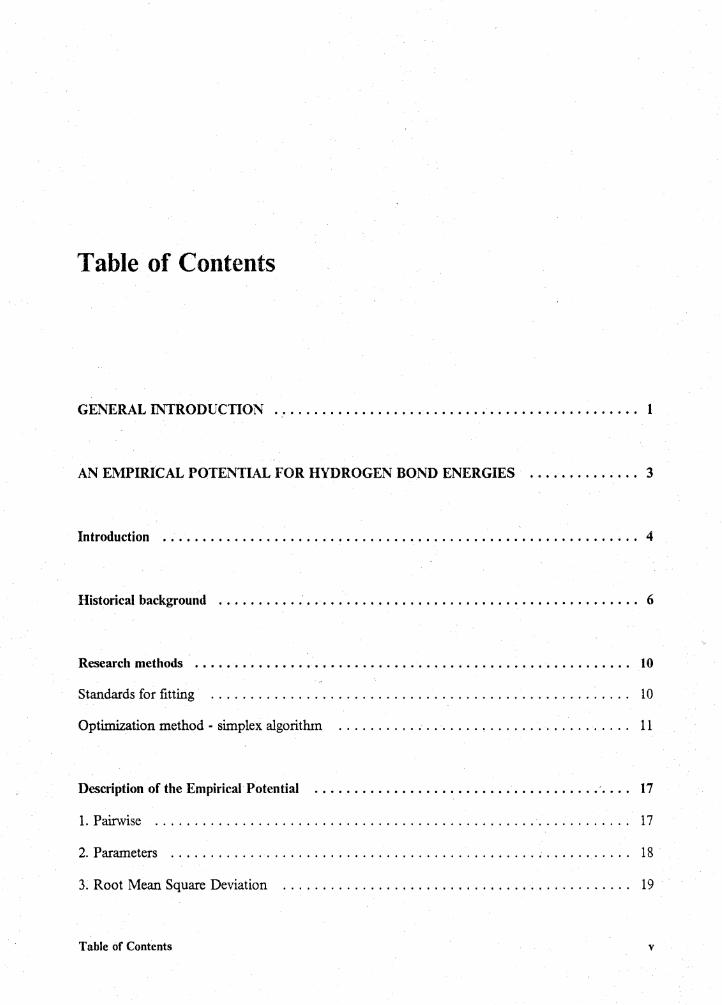
Table of Contents
GENERAL INTRODUCTION . . . . . . . . . . . . . . . . . . . . . . . . . . . . . . . . . . . . . . . . . . . . . . 1
AN EMPIRICAL POTENTIAL FOR HYDROGEN BOND ENERGIES . . . . . . . . . . . . . . 3
Introduction . . . . . . . . . . . . . . . . . . . . . . . . . . . . . . . . . . . . . . . . . . . . . . . . . . . . . . . . . . . . 4
Historical background .......... .' . . . . . . . . . . . . . . . . . . . . . . . . . . . . . . . . . . . . . . . . . . 6
Research methods ............................................ , . . . . . . . . . . 10
Standards for fitting . . . . . . . . . . . . . . . . . . . . . . . . . . . . . . . . . . . . . . . . . . . . . . . . . . . . . 10
Optimization method - simplex algorithm . . . . . . . . . . . . . . . . . . . . . . . . . . . . . . . . . . . . . 11
Description of the Empirical Potential . . . . . . . . . . . . . . . . . . . . . . . . . . . . . . . . . . . . . . . . 17
1. Pairwise . . . . . . . . . . . . . . . . . . . . . . . . . . . . . . . . . . . . . . . . . . . . . . . . . . . . . . . . . . . . . 17
2. Parameters . . . . . . . . . . . . . . . . . . . . . . . . . . . . . . . . . . . . . . . . . . . . . . . . . . . . . . . . . . 18
3. Root Mean Square Deviation . . . . . . . . . . . . . . . . . . . . . . . . . . . . . . . . . . . . . . . . . . . . 19
Table of Contents v
Applications . . . . . . . . . . . . . . . . . . . . . . . . . . . . . . . . . . . . • . . . . . . . . . . . . . . . . . . . . . . 27
Dimers: (H2 0)z, (NH3)z, NH3•H2 0 and (CH30H)2 ............................. 27
(H20)2 •••••••••••..••••••••••..••••••••••••••••••••••••••••••••••.• 27
(NH3 ) 2 •••••••••••••.••••••••••••••••••••••••••••••••••••••••••••••• 28
Mixed Dimers . . . . . . . . . . . . . . . . . . . . . . . . . . . . . . . . . . . . . . . . . . . . . . . . . . . . . . . . 31
Methanol Dimers . . . . . . . . . . . . . . . . . . . . . . . . . . . . . . . . . . . . . . . . . . . . . . . . . . . . . 31
Water oligomers . . . . . . . . . . . . . . . . . . . . . . . . . . . . . . . . . . . . . . . . . . . . . . . . . . . . . . . . 35
Non-cyclic trimers (H20h . . . . . . . . . . . . . . . . . . . . . . . . . . . . . . . . . . . . . . . . . . . . . . . 35
Cyclic (HzOh with C3 symmetry . . . . . . . . . . . . . . . . . . . . . . . . . . . . . . . . . . . . . . . . . . 36
Cyclic (Hz 0)4 with S4 symmetry . . . . . . . . . . . . . . . . . . . . . . . . . . . . . . . . . . . . . . . . . . 41
Ice-h . . . . . . . . . . . . . . . . . . . . . . . . . . . . . . . . . . . . . . . . . . . . . . . . . . . . . . . . . . . . . . . . 44
First Layer Lattice Energy . . . . . . . . . . . . . . . . . . . . . . . . . . . . . . . . . . . . . . . . . . . . . . . . . . 45
Second Layer Lattice Energy . . . . . . . . . . . . . . . . . . . . . . . . . . . . . . . . . . . . . . . . . . . . . . . 46
Third Layer Lattice Energy . : . . . . . . . . . . . . . . . . . . . . . . . . . . . . . . . . . . . . . . . . . . . . . . 48
Methanol crystal, ~-modification . . . . . . . . . . . . . . . . . . . . . . . . . . . . . . . . . . . .. . . . . . . . . 51
Conclusion . . . . . . . . . . . . . . . . . . . . . . . . . . . . . . . . . . . . . . . . . . . . . . . . . . . . . . . . . . . . 54
DETERMINATION OF THE ORIENTATION OF ANTHRACENE MOLECULES IN THE
UNIT CELL BY MEANS OF A REFRACTIVITY METHOD . . . . . . . . . . . . . . . . . . . . 56
Introduction . . . . . . . . . . . . . . . . . . . . . . . . . . . . . . . . . . . . . . . . . . . . . . . . . . . . . . . . . . . 57
Method .................................. , ........................... 59
Optimization of the Molecular Orientation . . . . . . . . . . . . . . . . . . . . . . . . . . . . . . . . . . . . . 63
Table of Contents vi
SOME AB INITIO CALCULATIONS INVOLVING TllE ACETONITRILE EXCHANGE
REACTION . . . . . . . . . . . . . . . . . . . . . . . . . • . . • . . . . . . . . . . . . . . . . . . . . . . • . . . . . . 69
Introduction . . . . • . . . . . . . . . . . . . . . . . . . . . . . . . · . . . . . • . . . . . . . . . . . . . . . . . • • . • . . 70
Results· ............................................................... 73
Discussion . . . . . . . . . . . . . . . . . . . . . . . . . . . . . . . . . . . . . . • . . . .. . . . • . . . . . . . . . . . . . 81
Appendix A. Cartesian coordinates of the methanol crystal . . ........................ · 83
References: • . . . . . . . . . . . . . . . . . . . . . . . . . . . . . . . . . . . . . . . . . . . . . . . . . . . . . . • . . . • 85
Table of Contents vii
List of Illustrations
Figure 1.
Figure 2.
Figure 3.
Figure 4.
Figure 5.
Figure 6.
Figure 7.
Figure 8.
Figure 9.
Configurations of (NH3)2 and NH3•H 20 adopted in optimization of empirical pa-rameters. . . . . . . . . . . . . . . . . . . . . . . . . . . . . . . . . . . . . . . . . . . . . . . . . . . . . 12
(NH3)2 and NH3•H20 Dimer Configurations by Type. . . . . . . . . . . . . . . . . . . . 13
Comparison of the curves calculated with different basis sets for the linear dimers of ammonia . . . . . . . . . . . . . . . . . . . . . . . . . . . . . . . . . . . . . . . . . . . . . . . . . . 15
Co?1pariso~ of the curves calculated with different basis sets for the cyclic duners of ammoma . . . . . . . . . . . . . . . . . . . . . . . . . . . . . . . . . . . . . . . . . . . . . . . . . . 16
Point charge models . . . . . . . . . . . . . . . . . . . . . . . . . . . . . . . . . . . . . . . . . . . . . 20
Geometry of water dimer . . . . . . . . . . . . . . . . . . . . . . . . . . . . . . . . . . . . . . . . . 29
Geometry of non-cyclic water trimer . . . . . . . . . . . . . . . . . . . . . . . . . . . . . . . . . 38
Geometry of cyclic water trimer . . . . . . . . . . . . . . . . . . . . . . . . . . . . . . . . . . . . 40
Geometry of water tetramer . . . . . . . . . . . . . . . . . . . . . . . . . . . . . . . . . . . . . . . 43
Figure 10. Pairwise relationship in lattice ice-h . . . . . . . . . . . . . . . . . . . . . . . . . . . . . . . . . 50
Figure 11. Structure of the ~-methanol crystal, projected along the c-axis of the orthorhombic cell. . . . . . . . . . . . . . . . . . . . . . . . . . . . . . . . . . . . . . . . . . . . . . . . . . . . . . . . . 53
Figure 12. The principal axis system of anthracene .............................. 68
Figure 13. Mechanisms suggested for the acetonitrile exchange reaction . . . . . . . . . . . . . . . . 72
Figure 14. Energy levels of the precusors, the intermediate and the transition states . . . . . . . 75
List of Illustrations viii
List of Tables
Table 1.
Table 2.
Table 3.
Table 4.
Table 5.
Table 6.
Comparisons of dimerization energies of (H2 0)z calculated . . . . . . . . . . . . . . . . . 21
Comparisons of dimerization energies of (NH3)z calculated . . . . . . . . . . . . . . . . . 23
Comparisons of dimerization energies of NH3•H20. calculated . . . . . . . . . . . . . . 25
Comparison of Experimental and Calculated Dimerization Energies . . . . . . . . . . . 30
Comparisons of Dimerization Energies of (NH3)z and NH3•H20. . . . . . . . . . . . 32
<;o_n;1parisons ?f dimerization energies of methanol dimers from empirical and ab 1111t10 calculations . . . . . . . . . . . . . . . . . . . . . . . . . . . . . . . . . . . . . . . . . . . . . . . 33
Table 7. Results for non-cyclic (H20h . . . . . . . . . . . . . . . . . . . . . . . . . . . . . . . . . . . . . . 37
Table 8. Results for C3 cyclic (H20)3 . . . . . . . . . . . . . . . . . . . . . . . . . . . . . . . . . . . . . . . 39
Table 9.
Table 10.
Table 11.
Table 12.
Table 13.
Table 14.
Table 15.
Results for S4 configuration of (H20)4 •••••••••..•.•••••••.••••••••••• 42
Energy comparison for the first layer of ice-h . . . . . . . . . . . . . . . . . . . . . . . . . . . 47
Lattice Energy of Ice-h . . . . . . . . . . . . . . . . . . . . . . . . . . . . . . . . . . . . . . . . . . . 49
Parameters for Bond Polarizabilities . . . . . . . . . . . . . . . . . . . . . . . . . . . . . . . . . . 64
Optimized Angle Set of Anthracene Molecules in their Monoclinic Unit Cell . . . . 65
Optimized geometrical parameters and energy values . . . . . . . . . . . . . . . . . . . . . . 76
Comparison of the energy levels using the various computational methods . . . . . . 80
List of Tables ix
General Introduction
The thesis is composed of three topics. The first is the study of an empirical potential for cal-
culating hydrogen bonding energies for systems involving oxygen and/or nitrogen. One purpose for
empirical potentials of this type could be to apply it to interaction involving large molecules such
as polypeptides and amino acids, where H-bonds are involved, for example, the hydrogen bonding
interaction in adenine-thymine and guanine-cytosine. Before the potential can be used for purposes
such as this, it is necessary to test the potentials for a variety of small molecular configurations.
As shown in the thesis, we have obtained reasonable results for small molecular configurations,
ice-h and methanol crystal when the potential parameters were optimized based on 6-31G"' basis
computations of 216 configurations of water, ammonia and mixed dimers. For large molecules, it
might be better to optimize the parameters based on crystal data as was done by Hagler. 1 The
empirical H-bonding potential can also be applied to liquid simulation studies. Jorgenson2 has
recently developed 12-6-3-1/ 12-6- l potentials which he has used for liquid simulation studies.
Taylor3 tl. developed a potential based on a dipole-dipole model to study carbohydrates.
Kroon-Batenburg et al.4 improved Taylor's potential especially in the bifurcated H-bonding con-
figurations of small molecules. An extra repulsive term was added to Kroon's potential and was
shown to play an important role to improve the energies of bifurcated configurations. In order to
avoid the point charge overlap catastrophe, switch functions have been used in Ben-Nairn-
General Introduction
Stillinger's potential.5 Our potential could also benefit from the use of the extra repulsive terms
and switch functions. We leave those improvements for future work.
In the second topic of the thesis, we have demonstrated the feasibility of optimizing the orien-
tation of an anisotropic molecuie such as anthracene in its crystal cell by means of fitting the di-
rectional refractivities of the molecule and that of the crystal. It might be useful as one of auxiliary
methods for crystal structure determination. It may also be useful in studies of liquid crystals.
In the third topic, we support the Walden inversion as the most likely mechanism for acetonitrile
exchange reaction through ab initio calculations and simple kinetic calculations. An addition-
rearrangement-elimination mechanism was suggested by Jay et al. 6 and 1,3 hydrogen shift in sol-
ution was suggested by Andrade et al .. 7 Our results are contrary to both Jay's and Andrade's
results.
General Introduction 2
An Empirical Potential for Hydrogen Bond Energies
An Empirical Potential for Hydrogen Bond Energies 3

Introduction
Morokuma et al.8 , Bene et al.9 and Kollman et al. 10a.have applied ab init1o calculations to de-
termination of the structure of the water dimer. The accuracy of the ab initio calculation of bond
lengths and bond angles now approach 0.02 A and 3 degrees, respectively, for small molecules.11
This makes the determination of molecular geometry possible where experiments are difficult or
even impossible to perform, such as the study of transition state structures.
However, it is prohibitively expensive to perform ab initio calculations to determine intermo-
lecular interaction energies of large monomers, simulations of liquid structure and estimates of
lattice energy based on H-bonding interactions. In some cases, such as biochemical molecules, it
is not possible at present to apply ab initio calculations. Empirical potentials provide useful alter-
natives. For example, Jorgensen2; 12«determined empirical potentials by fitting ab initio (ST0-3G)
SCF calculations on water, ammonia and methanol dimers, and then employed them in performing
Monte Carlo simulations of the liquid states of these materials.
In this thesis we developed an empirical potential which is aimed at fitting the hydrogen bonding
energies to ab initio results based on calculations which we performed using 6-31 G"' basis sets and
on MCYs' CI calculations.13 The fitting range chosen is for 0-0 distances from 2.8 A to 5.0 A.
This is within the most difficult range to determine the interaction energies of two water
Introduction 4
molecules.(page 239 of Ref. 14) The parameters involved in the empirical potential were optimized
using a simplex optimization method.15 The potential should be applicable to A-H--B systems
where A and Bare either 0 or N. We applied the potential to (H20)i, (NH3)i, NH3•H20, some
water oligomers, ice-h and methanol crystal. The potential should also be valuable in the esti-
mation of H-bonding energies, virial coefficients and configuration integration as well as in liquid
simulation where H-bonding is involved.
Introduction 5
Historical background
Stockmayer16 suggested a potential energy function between a pair of similar polar molecules.
It is composed of inverse power repulsion, inverse power attraction and permanent dipole-dipole
interaction:
-s -6 2 -3 U=lr -er -mr g
where s > 6, m is the permanent dipole moment, g = 2cos A cos B - sin A sin B cos C, A and B
are the inclinations of the two dipole axes to the intermolecular axis, and C is the azimuthal angle
between them. He applied the potential to water and ammonia, and calculated reasonable values
of the second Virial coefficients using both this potential and a hard sphere potential with an ad-
justed parameter. The differences between the observed and the calculated second virial coefficients
of ammonia and water are less than 3.5 cc/mol within the temperature range of 250K through 750K
when the diameters of the impenetrable spheres are 3.18A (ammonia), 3.16A (water) for hard
sphere models and 2.76A for a inverse-power model of water. Rawlinson has used the Stockmayer
potential to calculate the second and third virial coefficients for water vapor. 17 The interactions
involved are mainly hydrogen bonding energies. However, Hagler showed that the Stockmayer
potential does not fit the crystal data satisfactorily. 1 The aptness of the Stockmayer potential for
understanding condensed phases is questionable in that the minimum energy for a set of point
Historical background 6
dipoles is attained in the hexagonal close-packed crystal, not the tetrahedrally coordinated ice lattice.
In the wide variety of hydrate crystals loosely termed "clathrates", the water molecules stoutly
maintain the local tetrahedral coordination observed in ordinary ice. 5
Hagler1 suggested an amide hydrogen potential involving inverse sixth power attraction, inverse
power repulsion, partial charge coulomb interactions and a Morse potential term as the covalent
part of the hydrogen bond term. Attenuation of the Morse potential is accomplished by an expo-
nential angular dependence factor. All the parameters were fitted to experimental crystal data using
least-squares fitting.
Jorgensen21 12a.ritted his potentials to ST0-3G SCP.results for Monte Carlo simulation of water,
ammonium and methanol liquids. Those potentials are based on point charge. models. He used
12-6-3-1 potential functions for water and ammonia dimers and a 12-6-1 potential function for the
methanol dimer. (Recently he_ fitted his potential parameters to the experimental data for sulfur
compounds. 12~
, In order to simulate the geometries of carbohydrates, Taylor3~ 3b developed a potential fo.r the
O-H--0 hydrogen bond where the electrostatic component is calculated from the classical Jeans
equation for dipole-dipole interactions; Hill's equation is used for the van der Waals component;
an attenuation factor and van der Waals properties of the lone pairs are explicitly taken into ac-
count; and a Morse component and its attenuation factor are involved in the potential. Taylor's
potential is compatible with Allinger's molecular mechanics program (MMl).18 ci. This potential
yielded good results for water oligomers. However, it is suitable only for O-H--0 bonds, and it is
unnecessarily complicated. Kroon-Batenburg and Kanters4 developed an empirical O-H--0 hy-
drogen bond potential for MM2 force field calculations. Some modifications of the parameters
were made to the MM2 force field and an extra exponential term was added in order to improve
the bifurcated interaction of water dimers.
Historical background 7
A point charge model was adopted by Popkie et al) 9 to find an analytical expression which is
similar to that proposed by Bernal and Fowler.20 The parameters involved were optimized to fit
the Hartree· Pock energies. A potential surface was calculated and compared to the surfaces based
on Rowlinson's17 and Ben-Nairn & Stillinger's potential.5 A Monte Carlo simulation of liquid
water where 27 or 64 molecules of water were involved was performed using Popkie' s potential. 19
The results were in good agreement with the experimental data for liquid water, except that the
second peak of the radial pair correlation function for oxygen-oxygen was not obtained.
Based on Bjerrum's four-point-charge model of the water molecule,21 Ben-Nairn and Stillinger
suggested a tetrahedral charge model for the water molecule.5 The potential is composed of two
parts: the coulomb interactions among point charges between the different water molecules and the
Lennard-Jones 12-6 interactions. The coulomb term contains a switch factor with two distance
parameters, R and R', to avoid the charge overlap catastrophe. The distances of the charges from
the centeral oxygen nucleus was chosen to be 1.0A. The parameters of the Lennard-Jones potential
used were the same as for neon. ·The absolute charge quantity is kq, where q is the electron charge
and k is a parameter. When k=0.17, the known dipole moment for the free.water molecule was
reproduced. When k=0.19 and the other two parameters, Rand R', were chosen to be 2.0379A
and 3.1877 A, the energies of the water dimers with 2. 76A between two oxygens were as follows:
Symmetrical eclipsed -6.50 kcal/mol
Nonsymmetrical eclipsed -5.58 kcal/mol
Symmetrical staggered -5.34 kcal/mol
Nonsymmetrical staggered -6.13 kcal/~ol.
These data are compared with our results in Table 10.
Other empirical models suggested for intermolecular interactions between water monomers also
have been suggested.141 22 In general, point charge models have been shown to produce reasonable
results without complicated calculations. Among these were Verwey (1949), Pople (1951), Bernal
and Fowler (1933), Rawlinson (1951), Bjerrum (1951), Campbell (1952), and Cohan et al. (1962).22
The parameters they designed were adjusted to fit the experimental dipole moment. A multipole-
Historical background 8
expansion model was suggested by Coulson and Eisenberg (1966).22 Construction of a hydrogen
bonding potential by Gaussian functions was also suggested.14 In an empirical potential suggested
by Oies et aL,23 a "switch distance 0 of 3.3 A was adopted to distinguish a hydrogen bond from a
van der Waals interaction. When the distance is less than 3.3 A, the interaction is treated as a hy-
drogen bonding, otherwise it is considered as a van der Wa3.is interaction.
Application of empirical potential to the calculations of various water oligomers have also been . .
carried out.31 51 14
A variety of ab initio91 241 25 and empirical and semi-empirical methods31 221 26 have also been
used to calculate H-bonding energies of water oligomers and the lattice energies of ice-h.
Historical background 9
Research methods
Standards for fitting
Dimerization energies of 216 configurations, calculated using ab initio methods, were adopted
as standards for fitting the parameters of our empirical potential. Among the 216 configurations,
61 configurations of water dimers (H20)z were calculated by Matsuoka et al.13. We computed
dimerization energies for 85 configurations of the ammonia dimers (NH3)z and 70 configurations
of the mixed dimers NH3•H20 using 6-310+ basis sets. The configurations of the ammonia dimers
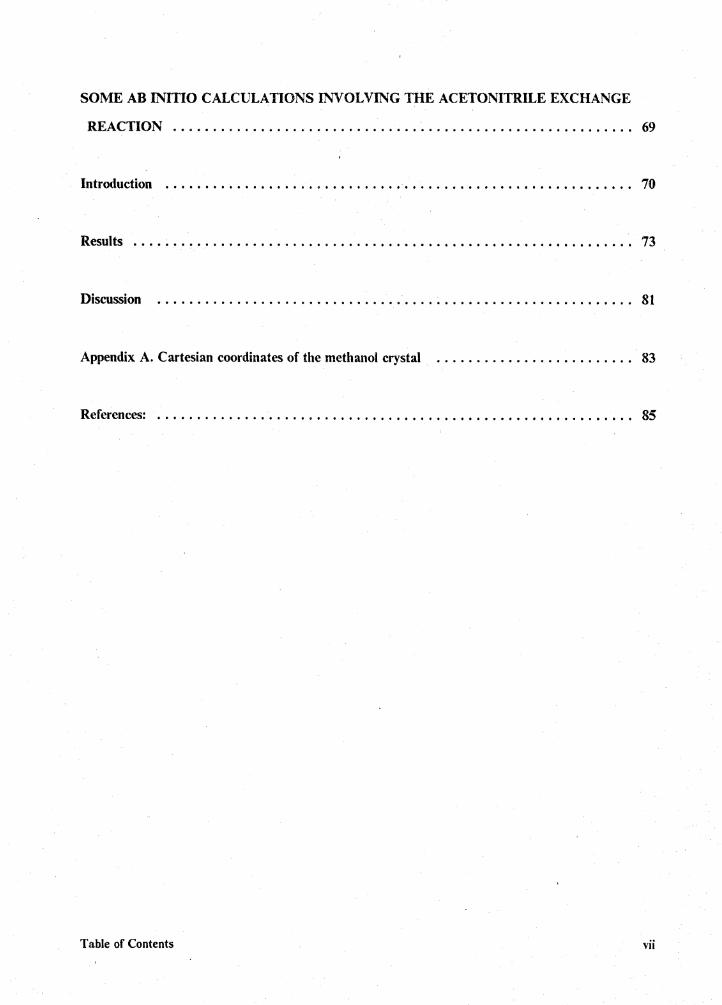
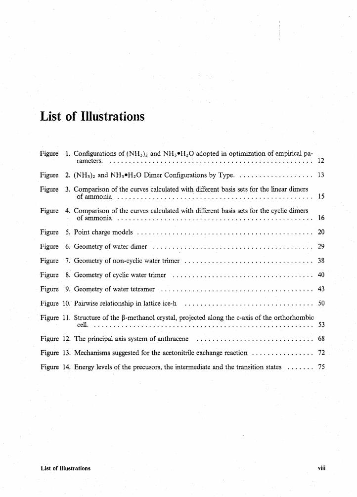
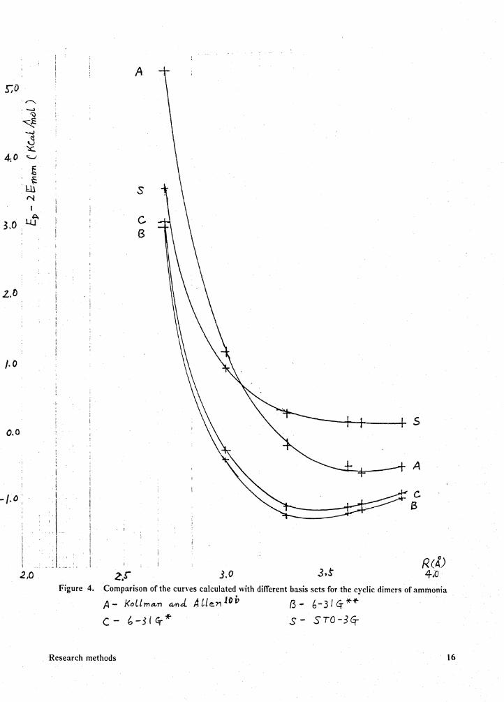
and mixed dimers are shown in Figure 1 and Figure 2. The 6-31G+ basis set was chosen based on
the comparison of the results from Allen as well as calculations we performed using 4-310, 6-310+
and 6-310++ basis sets as shown in Figures 3 and 4. In both figures, curves C (using 6-310"') and
B (using 6-310++) show nearly the same energies. But computations using the 6-310+ basis is less
expensive than that using the 6-310++ basis set. Curve S (ST0-30) is quite different from the
others in shape as well as in energies. This suggests that the results based on the ST0-30 basis set
used by Jorgensen2/ 2a are likely not suitable as criteria for standards. These ab initio results are
listed in Tables 1-3.
Research methods 10
Optimization method - sbnplex algorithm
By means of a fortran program "All", written by Viers and Schug, combined with a simplex
algorithm15 , we optimized the parameters, namely the charges and their locations in the monomer,
by fitting the calculated empirical energies to the cited ab initio results for the 216 dimer config-
urations. A function FN to be optimized to a mininum value was shown as follows:
FN = (61 x BESD of water dimers + 75 x BESD of anunonia dimers + 70 x BESD of mixed
dimers)/216.
where the weighting factors, 61, 75 and 70, are the numbers of the configurations for each kind of
dimers. The BESD is the best estimate of the standard deviation as follows:
BESD = .j'I.(Ei - Eab) 2 /(n - 1)
where n is the number of configurations, i.e. 61, 75 or 70 in each kind of dimers; Eab is the energy
of the ab initio result for each configuration and is considered as the "true" value; Ei is the calculated
empirical result for the same configuration. The monomer geometries of H20 and NH3 involved
in the optimization are the optimized geometrical results obtained from ab initio calculations using
6-31G* basis sets. For simplicity, it is assumed that the monomers retain their geometry in their
dimers or oligomers.
Research methods 11
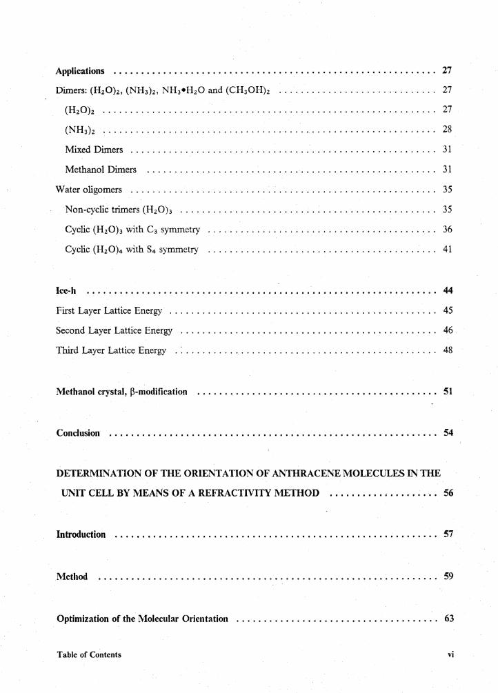
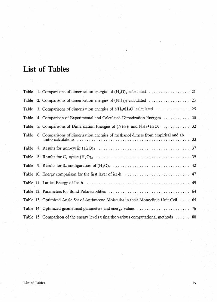
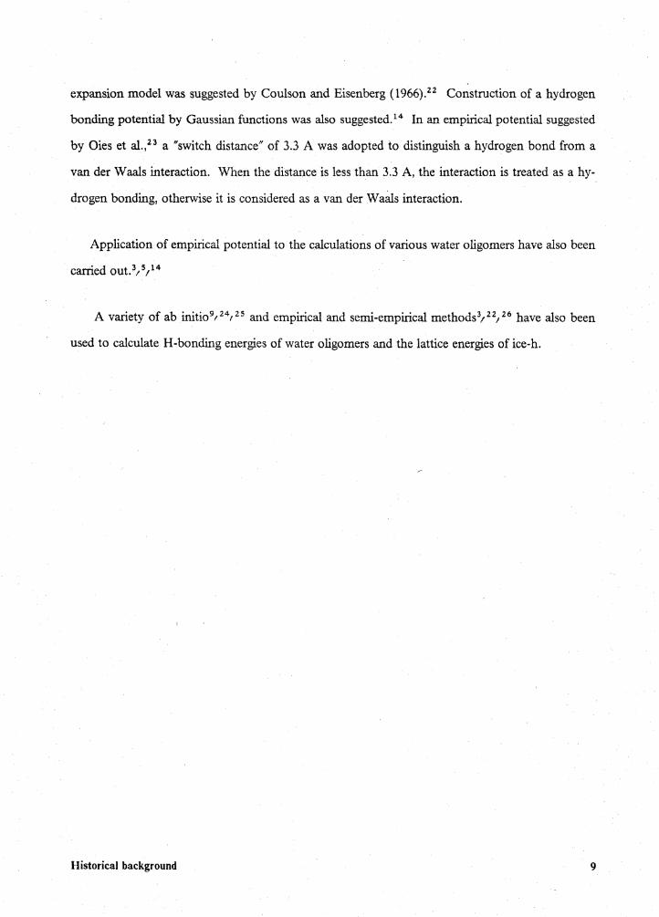
Linear types: B, Bl I B2 Bifurcated types: A, Al I A2
A Al A2 B Bl B' B2 c Cl C' D Dl Dll D'
Cyclic types: D, Dl
8 (deg) ¢ (deg) 0. 0. 0.
68.3 0. 68.3 0. 68.3 30, 60, 90 52.8 0. 90. 0. 90. 0. 90. 30, 60, 90
128.5 0. 128.5 0. 128.5 0. 128.5 30 I 60, 90
Fig. 1 Configurations of (NH3 ) 2 and :t.1H3 •H2o adopted in optimization of empirical parameters.
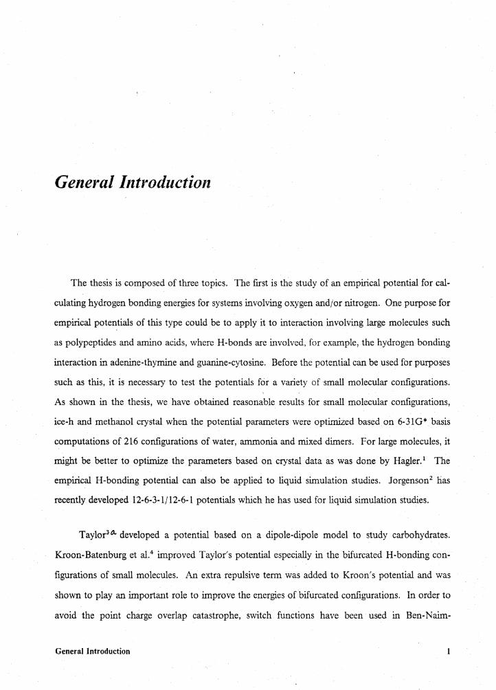
12
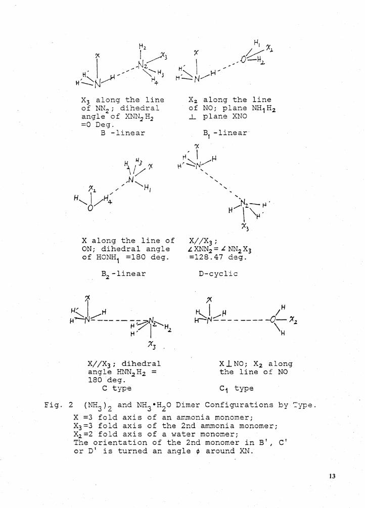
X3 along the line of NN2 ; dihedral angle of XNN2 H2 =O Deg.
B -linear
X along the line of ON; dihedral angle of HONH1 =180 deg.
B2 -linear
X//X3; dihedral angle HNN2 H2 = 180 deg.
C type
X2 along the line of NO; plane NH1H2 J_ plane XNO
B1 -linear
'X t1, \ H
\1~~,"1/ ' ' ' '
X//X3 ;
' '
LXNN2 = ~ NN2 X3 =128.47 deg.
D-cyclic
;x. ~i_,J .......-H /H rr-~--- - ---- -0\ Xz
H
X l. NO; X2 along the line of NO
Fig. 2 (NH3 ) 2 and NH3 •H2o Dimer Configurations by ~ype. X =3 fold axis of an arr~onia monomer; x3=3 fold axis of the 2nd ammonia monomer; X2 =2 fold axis of a water monomer; The orientation of the 2nd monomer in B', C' or D' is turned an angle ¢ around XN.
13
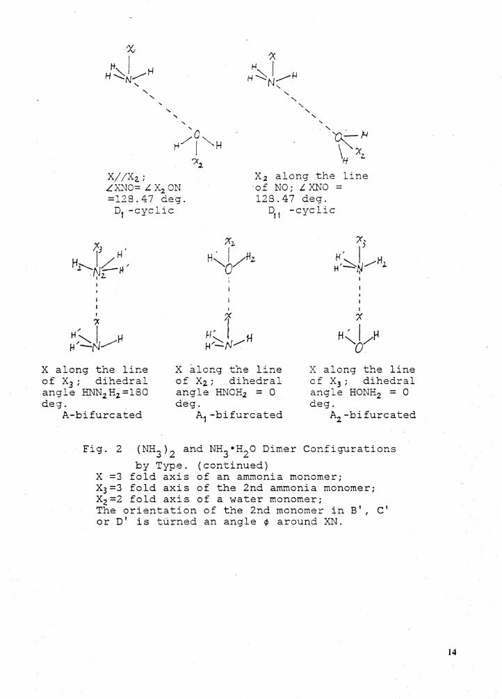
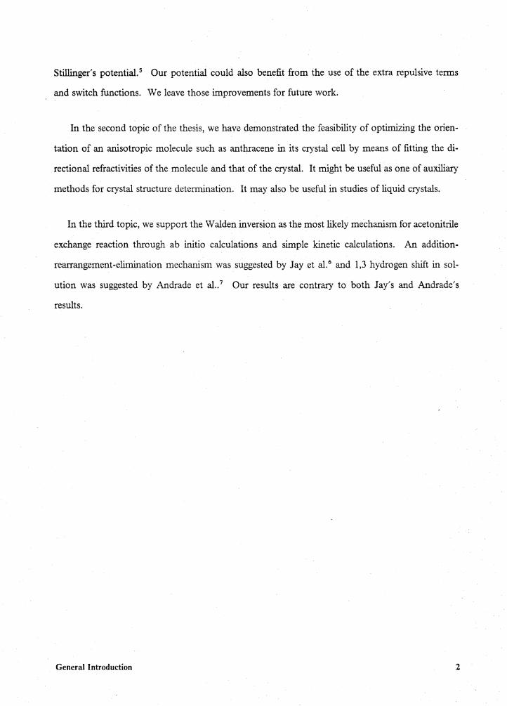
' . ~~
\ Xz. H
X//X2.; L X..\JO= L X2 ON =128.47 deg.
X2 along the line of NO; L. XNO = 128_.47 deg.
D1 -cyclic
X along the line of X3 ; dihedral angle HNN2 H2 =180 deg.
A-bifurcated
D 1 . 11 -cyc .... ic
x along the line of X2; dihedral angle HNOH2 = 0 deg.
A1 -bifurcated
x, f1' I H H'~t:J/ ).
I I
I
I
'X
H~ I /ri 0
X along the line of X3 ; dihedral angle HONH2 = 0 deg.
A2 -bifurcated
Fig. 2 (NH3 ) 2 and NH3 •H2o Dimer Configurations by Type. (continued)
X =3 fold axis of an ammonia monomer; X3=3 fold axis of the 2nd ammonia monomer; X2 =2 fold axis of a water monomer; The orientation of the 2nd monomer in B', C' or D' is turned an angle ¢ around XN.
14

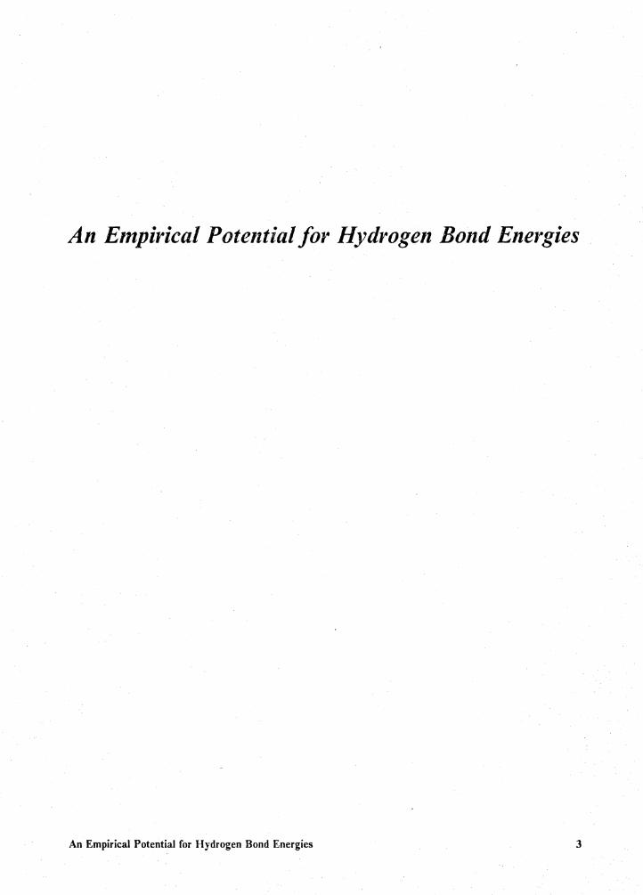
J.0:. , ......... _, :o ~ J :::,c
2.0 .'--' s :u? . "4
I 'A
1.0 .l.L.i
o.o
. /, (J
-2.D
-3.0
I i
2.0
I I
.l
A
B c
s s A
~
R(A) 3.0 4.0
Figure 3. '.'omparison of the curves calculated with different basis sets for the linear dimers of ammonia
A - Kollma-n AYl.::l AUen 1°h B- 6-31 ~** c. - 6 -31 f:r*' S- ST0-3C:,-
!fr search m r hods 15
!;;D . ,,.--... ..........
~ ~ \..)
~ 4:0 <;._;
s ' ~
hll ~
I
3.0' uf'
2..D
/. 0
o.o
-/.0:
2,0
I i . J __ _
A
s
c B
s
A
c 6
3.0 Figure 4. Comparison of the curves calculated with different basis sets for the cyclic dimers of ammonia
A- kollma-n Cvrtd. Alle.n 10 b (3- b-3/q.**" C - b -3 i Gr*" S - S TO -3 6r
Research methods 16
Description of the E1npirical Potential
1. Pairwise
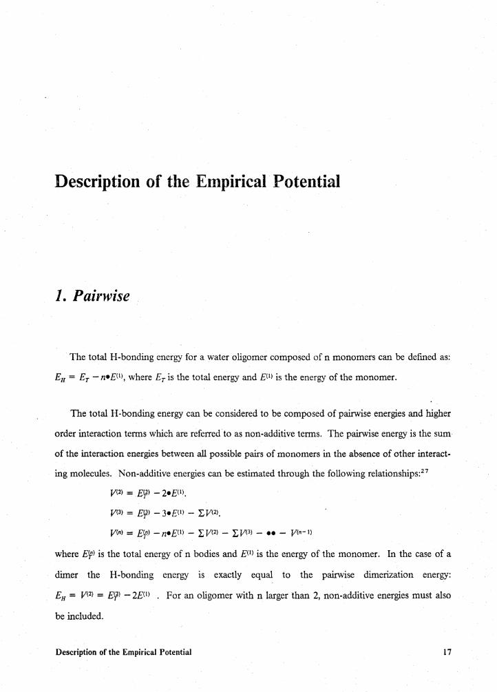
The total H-bonding energy for a water oligomer composed of n monomers can be defmed as:
EH = Er - n•£<1), where Er is the total energy and £<1) is the energy of the monomer.
The total H-bonding energy can be considered to be composed of pairwise energies and higher
order interaction terms which are referred to as non-additive terms. The pairwise energy is the sum
of the interaction energies between all possible pairs of monomers in the absence of other interact-
ing molecules. Non-additive energies can be estimated through the following relationships:27
v<2> = E~> - 2•£<1).
V(3) = E9) - 3•£(t) - I: V(2l.
v<n> = Efp> - n•£(l) - I: v(2) - I: V<3) - •• - v<n-1)
where Erp> is the total energy of n bodies and £<1> is the energy of the monomer. In the case of a
dimer the H-bonding energy is exactly equal to the pairwise dimerization energy:
EH = V<2> = E~> -2£<1> • For an oligomer with n larger than 2, non-additive energies must also
be included.
Description of the Empirical Potential 17
2. Parameters
Our empirical potential for the interaction between a pair of monomers is composed of van der
Waals interactions and electrostatic contributions.
Van der Waals interactions between all pairs of atoms in different molecules are computed using
the Hill equations (1) and (la) with parameters for 0, N and H taken from Allinger's MM2
program.18b Although Allinger uses van der Waals interactions involving lone pair pseudoatoms,
these are not included in our intermolecular potential.
Evvw = E(2.9 x 10⁵ exp( -12.5/P) - 2.25P6),
Evvw = E x 336.176?2,
where P = r*/R
R = effective internuclear distance
if p < 3.311 (1)
if P > 3.311 (la)
r* = summation of the VDW radii of the two atoms involved, in A
E = geometrical average of the "hardness" of the two atoms, in kcal/mol
r* and i:; can be calculated based on Allinger's table. 16
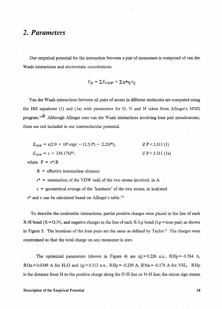
To describe the coulombic interactions, partial positive charges were placed in the line of each
X-H bond (X = O,N), and negative charges in the line of each X-Lp bond (Lp =lone pair) as shown
in Figure 5. The locations of the lone pairs are the same as defined by Taylor. 3 The charges were
constrained so that the total charge on any monomer is zero.
The optimized parameters (shown in Figure 4) are iql = 0.226 a.u., RHp = -0.584 A,
ROn=0.0349 A for H20 and iqi=0.312 a.u., RHp=-0.239 A, RNn=-0.178 A for NH3. RHp
is the distance from H to the positive charge along the 0-H line or N-H line; the minus sign means
Description of the Empirical Potential 18
that the charge lies outside the 0-H bond or N-H bond. ROn is the distance between 0 and the
negative charge along the line from 0 to the center of a lone pair. Equivalent meanings are used
for the remaining parameters.
3. Root Mean Square Deviation
The RMS deviation of the 216 configurations is 0.9 kcal/mol, where the ab initio results of
Matsuoka and those of 6-31G* are adopted as standards. The RMS deviation using Taylor po-
tential is 1.42 kcal/mol and that of Kroon's is 0.6 kcal/mol for the 66 configurations of water
dimers. Our parameters were optimized based on 216 configurations of water dimers, ammonia
dimers and mixed dimers. Using these parameters, the RMS deviation of the ab initio versus em-
pirical interaction energies from our potential is 0.87 kcal/mol for 61 configurations of the water
dimers.
In a separate optimization, the resulted parameters of CH30H monomer are also listed in Fig.
5. The RMS deviation is 0.5 kcal/mol for 61 configurations of methanol dimers.
Description of the Empirical Potential 19
L L
~-4 /o~
H H t} +1
L !
H/f~H +( H ~}
~r
L L
H -~J( ~c---o ~
H H/ ~H +'6-
L - lone pair electrons
!qi = 0.226 a.u.
RHp =-0.584 A
ROn = 0.0349 A
!qi = 0.312 a.u.
RHp =-0.239 A
RNn =-0.178 A
L - lone pair electrons
!qi = 0.20 a.u.
lq' I = 0.20 a.u.
ROn = 0.076 A
RHp =-0.58 A
RCp =-0.72 A
Fig. 5 Point charge models
20
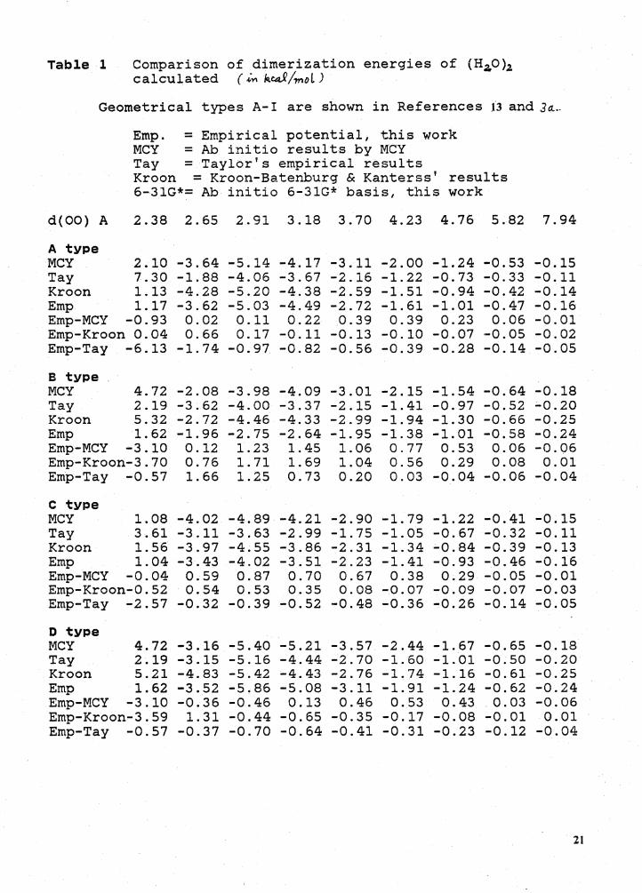
Table 1 Comparison of dimerization energies of (Hz0)2 calculated ( ,i,,, kca.Q/moL)
Geometrical types A-I are shown in References 13 and Ja...-
Emp. = Empirical potential, this work MCY = Ab initio results by MCY Tay =Taylor's empirical results Kroon = Kroon-Batenburg & Kanterss' results 6-31G*= Ab initio 6-31G* basis, this work
d(OO) A 2.38 2.65 2.91 3.18 3.70 4.23 4.76 5.82 7.94
A type MCY 2.10 Tay 7.30 Kroon 1.13 Emp 1.17 Emp-MCY -0.93 Emp-Kroon 0.04 Emp-Tay -6.13
B type MCY 4.72 Tay 2.19 Kroon 5.32 Emp 1. 62 Emp-MCY -3.10 Emp-Kroon-3.70 Emp-Tay -0.57
c type MCY 1.08 Tay 3.61 Kroon 1. 56 Emp 1.04 Emp-MCY -0.04 Emp-Kroon-0.52 Emp-Tay -2.57
D type MCY 4.72 Tay 2.19 Kroon 5.21 Emp 1. 62 Emp-MCY -3.10 Emp-Kroon,...3.59 Emp-Tay -0.57
-3.64 -1.88 -4.28 -3.62 0.02 0.66
-1. 74
-2.08 -3.62 -2.72 -1. 96 0.12 0.76 1. 66
-4.02 -3.11 -3.97 -3.43 0.59 0.54
-0.32
-3.16 -3.15 -4.83 -3.52 -0.36 1. 31
-0.37
-5.14 -4.06 -5.20 -5.03 0.11 0.17
-0.97
-3.98 -4.00 -4.46 -2.75
1.23 1. 71 1.25
-4.89 -3.63 -4.55 -4.02 0.87 0.53
-0.39
-5.40 -5.16 -5.42 -5.86 -0.46 -0.44 -0.70
-4.17 -3.67 -4. 38 -4.49 0.22
-0.11 -0.82
-4.09 -3.37 -4.33 -2.64
1.45 1. 69 0.73
-4.21 -2.99 -3.86 -3.51 0.70 0.35
-0.52
-5.21 -4.44 -4.43 -5.08 0.13
-0.65 -0.64
-3.11 -2.16 -2.59 -2.72 0.39
-0.13 -0.56
-3.01 -2.15 -2.99 -1. 95 1.06 1.04 0.20
-2.90 -1. 75 -2.31 -2.23 0.67 0.08
-0.48
... 3 .57 -2.70 -2.76 -3.11 0.46
-0.35 -0.41
-2.00 -1.22 -1.51 -1. 61 0.39
-0.10 -0.39
-2.15 -1.41 -1.94 -1. 38 0.77 0.56 0.03
-1. 79 -1. 05 -1. 34 -1.41 0.38
-0.07 -0.36
-2.44 -1. 60 -1. 74 -1. 91 0.53
-0.17 -0.31
-1.24 -0.73 -0.94 -1.01 0.23
-0.07 -0.28
-1. 54 -0.97 -1.30 -1. 01 0.53 0.29
-0.04
-1.22 -0.67 .;..o. 84 -0.93 0.29
-0.09 -0.26
-1. 67 -1.01 -1.16 -1.24 0.43
-0.08 -0.23
-0.53 -0.33 -0.42 -0.47 0.06
-0.05 -0.14
-0.64 -0.52 -0.66 -0.58 0.06 0.08
-0.06
-0.41 -0.32 -0.39 -0.46 -0.05 -0.07 -0.14
-0.65 -0.50 -0.61 -0.62
0.03 -0.01 -0.12
-0.15 -0.11 -0.14 -o .16 -0.01 -0.02 -0.05
-0.18 -0. 20 -0.25 -0.24 -0.06 0.01
-0.04
-0.15 -0.11 -0.13 -0.16 -0.01 -0.03 -0.05
-0.18 -0.20 -0.25 -0.24 -0.06
0.01 -0.04
21
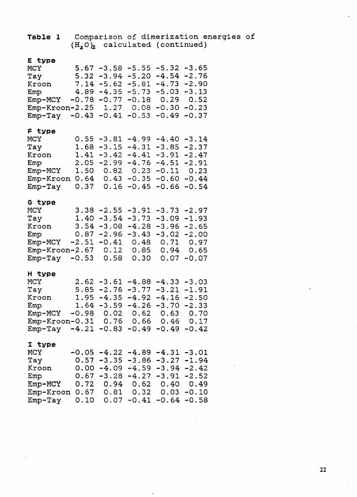
Table 1 Comparison of dimerization energies of (HaO).,a calculated (continued)
E type MCY 5.67 -3.58 -5.55 -5.32 -3.65 Tay 5.32 -3.94 -5.20 -4.54 -2.76 Kroon 7.14 -5.62 -5.81 -4.73 -2.90 Emp 4.89 -4.35 -5.73 -5.03 -3.13 Emp-MCY -0.78 -0.77 -0.18 0.29 0.52 Emp-Kroon-2.25 1.27 0.08 -0.30 -0.23 Emp-Tay -0.43 -0.41 -0.53 -0.49 -0.37
F type MCY 0.55 -3.81 -4.99 -4.40 -3.14 Tay 1. 68 -3.15 -4.31 -3.85 -2.37 Kroon 1. 41 -3.42 -4.41 -3.91 -2.47 Emp 2.05 -2.99 -4.76 -4.51 -2.91 Emp-MCY 1. 50 0.82 0.23 -0.11 0.23 Emp-Kroon 0.64 0.43 -0.35 -0.60 -0.44 Emp-Tay 0.37 0.16 -0.45 -0.66 -0.54
G type MCY 3.38 -2.55 -3.91 -3.73 -2.97 Tay 1.40 -3.54 -3.73 -3.09 -1.93 Kroon 3.54 -3.08 -4.28 -3.96 -2.65 Emp 0.87 -2.96 -3.43 -3.02 -2.00 Emp-MCY -2.51 -0.41 0.48 0.71 0.97 Emp-Kroon-2.67 0.12 -o. 85 0.94 0.65 Emp-Tay -0.53 0.58 0. 30 0.07 -0.07
H type MCY 2.62 -3.61 -4.88 -4.33 -3.03 Tay 5.85 -2.76 -3.77 -3.21 -1.91 Kroon 1.95 -4.35 -4.92 -4.16 -2.50 Emp 1. 64 -3.59 -4.26 -3.70 -2.33 Emp-MCY -0.98 0.02 0.62 0.63 0.70 Emp-Kroon-0.31 0.76 0.66 0.46 0.17 Emp-Tay -4. 21 -0.83 -0.49 -0.49 -0.42
I type MCY -0.05 -4.22 -4.89 -4. 31 -3.01 Tay 0.57 -3.35 -3.86 -3.27 -1.94 Kroon 0.00 -4.09 -4.59 -3.94 -2.42 Emp 0.67 -3.28 -4. 27 -3.91 -2.52 Emp-MCY 0.72 0.94 0.62 0.40 0.49 Emp-Kroon 0.67 0.81 0.32 0.03 -0.10 Emp-Tay 0.10 0.07 -0.41 -0.64 -0.58
22
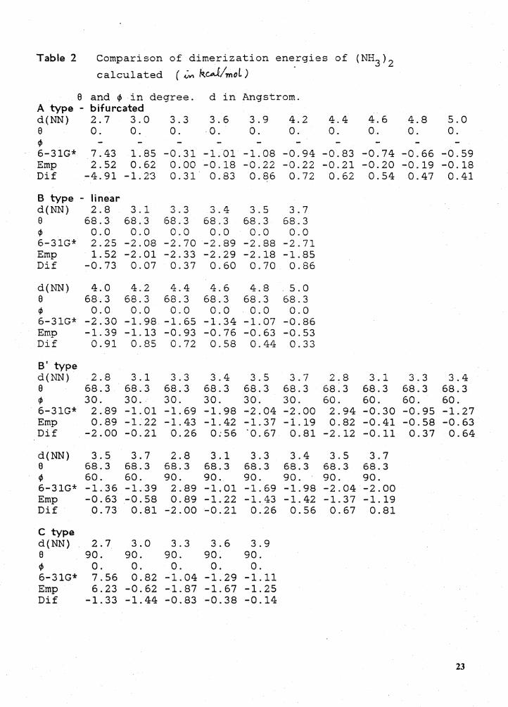
Table 2 Comparison of dimerization energies of (NH3)2 calculated ( ~"" kwlmoL)
8 and 'Ii in degree. d in Angstrom. A type - bifurcated d(NN) 2.7 3.0 3.3 3.6 3.9 4.2 4.4 4.6 4.8 5.0 8 0. 0. 0. 0. 0. 0. 0. 0. 0. 0. cp 6-31G* 7.43 1. 85 -0.31 -1. 01 -1.08 -0.94 -0.83 -0.74 -0.66 -0.59 Emp 2.52 0.62 0.00 -0.18 -0.22 -0.22 -0.21 -0.20 -0.19 -0.18 Dif -4.91 -1.23 0.31 0.83 0.86 0.72 0.62 0.54 0.47 0.41
B type - linear d(NN) 2.8 3.1 3.3 3.4 3.5 3.7 8 68.3 68.3 68.3 68.3 68.3 68.3 ¢ 0.0 0.0 0.0 0.0 0.0 0.0 6-31G* 2.25 -2.08 -2.70 -2.89 -2.88 -2.71 Emp 1.52 -2.01 -2.33 -2.29 -2.18 -1.85 Dif -0.73 0.07 0.37 0.60 0.70 0.86
d(NN) 4.0 4.2 4.4 4.6 4.8 5.0 a 68.3 68.3 68.3 68.3 68.3 68.3 ¢ 0.0 0.0 0.0 0.0 0.0 0.0 6-31G* -2.30 -1.98 -1. 65 -1. 34 -1. 07 -0.86 Emp -1. 39 -1.13 -0.93 -0.76 -0.63 -0.53 Dif 0.91 0.85 0.72 0.58 0.44 0.33
B' type d(NN) 2.8 3.1 3.3 3.4 3.5 3.7 2.8 3.1 3.3 3.4 8 68.3 68.3 68.3 68.3 68.3 68.3 68.3 68.3 68.3 68.3 ¢ 30. 30. 30. 30. 30. 30. 60. 60. 60. 60. 6-31G* 2.89 -1.01 -1. 69 -1. 98 -2.04 -2.00 2.94 -0.30 -0.95 -1.27 Emp 0.89 -1.22 -1.43 -1.42 -1. 37 -1.19 0.82 -0.41 -0.58 -0.63 Dif -2.00 -0.21 0.26 0:56 ·o.67 0.81 -2.12 -0.11 0.37 0.64
d(NN) 3.5 3.7 2.8 3.1 3.3 3.4 3.5 3.7 a 68.3 68.3 68.3 68.3 68.3 68.3 68.3 68.3 ¢ 60. 60. 90. 90. 90. 90. 90. 90. 6-31G* -1. 36 -1. 39 2.89 -1.01 -1. 69 -1.98 -2.04 -2.00 Emp -0.63 -0.58 0.89 -1.22 -1.43 -1.42 -1. 37 -1.19 Dif 0.73 0.81 -2.00 -0.21 0.26 0.56 0.67 0.81
C type d(NN) 2.7 3.0 3.3 3.6 3.9 8 90. 90. 90. 90. 90. ¢ 0. 0. 0. 0. 0. 6-31G* 7.56 0.82 -1.04 -1. 29 -1.11 Emp 6.23 -0.62 -1. 87 -1. 67 -1. 25 Dif -1. 33 -1.44 -0.83 -0.38 -0.14
23
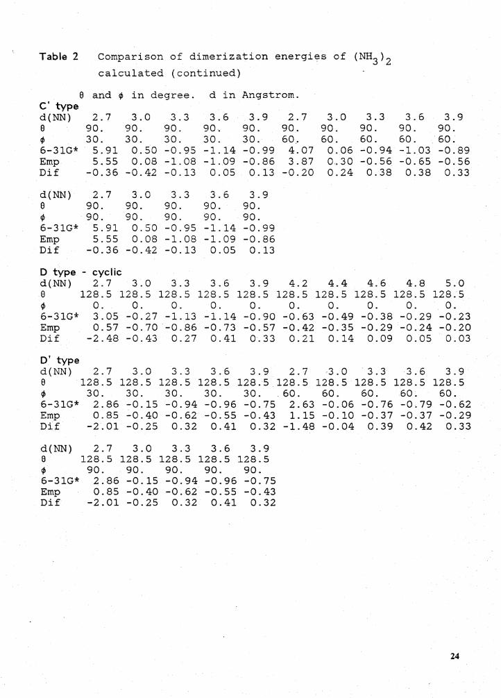
Table 2 Comparison of dimerization energies of (NH3)2 calculated (continued)
e and ¢ in degree. d in Angstrom. C' type d(NN) 2.7 3.0 3.3 3.6 3.9 2.7 3.0 3.3 3.6 3.9 e 90. 90. 90. 90. 90. 90. 90. 90. 90. 90. ¢ 30. 30. 30. 30. 30. 60 .. 60. 60. 60. 60. 6-31G* 5.91 0.50 -0.95 -1.14 -0.99 4.07 0.06 -'0.94 -1. 03 -0.89 Emp 5.55 0.08 -1. 08 -1.09 -0.86 3.87 0 .. 30 -0.56 -0.65 -0.56 Dif -0.36 -0.42 -0.13 0.05 0.13 -0.20 0.24 0.38 0.38 0.33
d(NN) 2.7 3.0 3.3 3.6 3.9 e 90. 90. 90. 90. 90. ¢ 90. 90. 90. 90. 90. 6-31G* 5.91 0.50 -0.95 -1.14 -0.99 Emp 5.55 0.08 -1.08 -1.09 -0.86 Dif -0.36 -0.42 -0.13 0.05 0.13
D type - cyclic d(NN) 2.7 3.0 3.3 3.6 3.9 4.2 4.4 4.6 4.8 5.0 e 128.5 128.5 128.5 128.5 128.5 128. 5 128.5 128. 5 128.5 128. 5 ¢ 0. 0. 0. 0. 0. 0. 0. 0. 0. 0. 6-31G* 3.05 -0.27 -1.13 -1.14 -0.90 -0.63 -0.49 -0.38 -0.29 -0.23 Emp ·o.57 -0.70 -0.86 -0.73 -0.57 -0.42 -0.35 -0.29 -0.24 -0.20 Dif -2.48 -0.43 0.27 0.41 0.33 0.21 0.14 0.09 0.05 0.03
D' type d(NN) 2.7 3.0 3.3 3.6 3.9 2.7 3.0 3.3 3.6 3.9 e 128.5 128.5 128.5 128.5 128.5 128.5 128.5 128.5 128.5 128.5 ¢ 30. 30. 30. 30. 30. 60. 60. 60. 60. 60. 6-31G* 2.86 -0.15 -0.94 -0.96 -0.75 2.63 -0.06 -0.76 -0.79 -0.62 Emp 0.85 -0.40 -0.62 -0.55 -0.43 1.15 -0.10 -0.37 -0.37 -0.29 Dif -2.01 -0.25 0.32 0.41 0.32 -1.48 -0.04 0.39 0.42 0.33
d(NN) 2.7 3.0 3.3 3.6 3.9 e 128.5 128.5 128.5 128.5 128.5 ¢ 90. 90. 90. 90. 90. 6-31G* 2. 86 -0.15 -0.94 -0.96 -0.75 Emp 0.85 -0.40 -0.62 -0.55 -0.43 Dif -2.01 -0.25 0.32 0.41 0.32
24
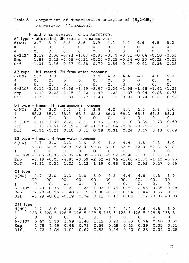
Table 3 Comparison of dimerization energies of (H2 o•NH3 )
calculated ( ~ kW/mol)
9 and ¢ in degree. d in Angstrom. A1 type - bifurcated, 3H from ammonia monomer d(NO) 2.7 3.0 3.3 3.6 3.9 4.2 4.4 4.6 4.8 5.0 9 0. 0. 0. 0. 0. 0. 0. 0. 0. 0. ¢ 0. 0. 0. 0. 0. 0. 0. 0. 0. 0. 6-31G* 3.19 0.06 -0.93 -1.07 -0.95 -0.79 -0.71 -0.64 -0.58 -0.53 Emp 1. 88 0.42 -0.06 -0.21 -0.25 -0.25 -0.24 -0.23 -0.22 -0.21 Dif -1. 31 0. 36 0.87 0.86 0.70 0.54 0.47 0.41 0.36 0.32
A2 type - bifurcated, 2H from water monomer d(ON) 2.7 3.0 3.3 3.6 3.9 4.2 4.4 4.6 4.8 5.0 9 0. 0. 0. 0. 0. 0. 0. 0. 0. 0. ¢ 0. 0. 0. 0. 0. 0. 0. 0. 0. 0. 6-31G* 0.14 -3.35 -3.96 -3.59 -2.97 -2.34 -1. 98 -1.68 -1.44 -1. 25 Emp -1.19 -2.23 -2.15 -1.82 -1.49 -1.22 -1.07 -0.94 -0.83 -0.73 Dif -1. 33 1.12 1. 81 1. 77 1. 48 1.12 0.91 0.74 0.61 0.52
Bl type - linear, H from ammonia monomer d(NO) 2.7 3.0 3.3 3.6 3.9 4.2 4.4 4.6 4.8 5.0 9 68.3 68.3 68.3 68.3 68.3 68.3 68.3 68.3 68.3 68.3 ¢ 0. 0. 0. 0. 0. 0. 0. 0. 0. 0. 6-31G* 3.44 -1. 30 -2.22 -2.11 -1. 76 -1. 35 -1.10 -0.89 -0.73 -0.60 Emp 3.13 -1.51 -2.12 -1.80 -1. 38 -1.04 -0.86 -0.72 -0.60 -0.51 Dif -0.31 -0.21 0.10 0.31 0.38 0.31 0.24 0.17 0.13 0.09
B2 type - linear, H from water monomer d(ON) 2.7 3.0 3.3 3.6 3.9 4.2 4.4 4.6 4.8 5.0 9 52.8 52.8 52.8 52.8 52.8 52.8 52.8 52.8 52.8 52.8 ¢ 0. 0. 0. 0. 0. 0. 0. 0. 0. 0. 6-31G* -3.86 -6.35 -5.87 -4.82 -3.81 -2.92 -2.40 -1. 95 -1.59 -1. 31 Emp -5.18 -6.03 -4.85 -3.59 -2.62 -1.94 -1.60 -1. 33 -1.12 -0.95 Dif -1.32 0.32 1.02 1.23 1.19 0.98 0.80 0.62 0.47 0. 36
Cl type d(NO) 2.7 3.0 3.3 3.6 3.9 4.2 4.4 4.6 4.8 5.0 9 90. 90. 90. 90. 90. 90. 90. 90. 90. 90. ¢ 0. 0. 0. 0. 0. 0. 0. 0. 0. 0. 6-31G* 3.49 -0.35 -1.21 -1. 23 -1.02 -0.76 -0.59 -0.46 -0.35 -0.28 Emp 2.20 -0.96 -1.40 -1.19 -0.90 -0.66 -0.54 -0.44 -0.37 -0.31 Dif -1.29 -0.61 -0.19 0.04 0.12 0.10 0.05 0.02 -0.02 -0.03
011 type d (.NO) 2.7 3.0 3.3 3.6 3.9 4.2 4.4 4.6 4.8 5.0 9 128.5 128.5 128.5 128.5 128.5 128.5 128.5 128.5 128.5 128.5 ¢ 0. 0. 0. 0. o. 0. 0. 0. 0. 0. 6-31G* 6.47 3.33 1. 99 1. 40 1.12 0.93 0.83 0.74 0.66 0.59 Emp 2.75 1. 49 0.98 0.73 0.59 0.49 0.43 0.39 0.35 0.31 Dif. -3.72 -1. 84 -1. 01 -0.67 -0.53 -0.44 -0.40 -0.35 -0.31 -0.28
25
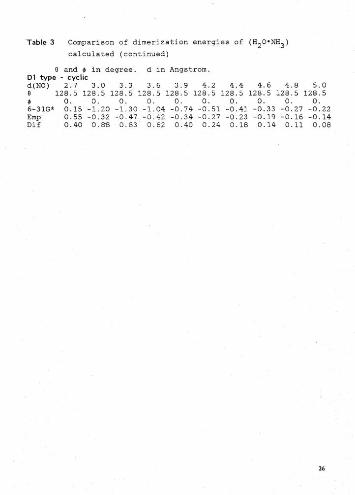
Table 3
a
Comparison of dimerization energies of (H20•NH3 ) calculated (continued)
and "'
in degree. d in Angstrom. Dl type - cyclic d(NO) 2.7 3.0 3.3 3.6 3.9 4.2 4.4 4.6 4.8 a 128.5 128.5 128.5 128.5 128.5 128.5 128.5 128.5 128. 5
"' 0. 0. 0. 0. 0. 0. 0. 0. 0.
6-31G* 0.15 -1.20 -1. 30 -1.04 -0.74 -0.51 -0.41 -0.33 -0.27 Emp 0.55 -0.32 -0.47 -0.42 -0.34 -0.27 -0.23 -0.19 -0.16 Dif 0.40 o.ss 0.83 0.62 0.40 0. 24 0.18 0.14 0.11
5.0 128.5
0. -0.22 -0.14 0.08
26
Applications
The geometrical parameters of the water dimer as determined from a supersonic nozzle beam
experiment are d(0-0) = 2.98± 0.01 A; a= 58± 6 degree. 28
Using the experimental structure discussed above along with the empirical potential described
previously, the calculated dimerization energy for (H.z0)2 is -5.74 kcal/mol. This is based on
d(O-H) = 0.9572 A, HOH= 104.52 degree, d(0-0) = 2.981 A and a= 58.6 degree (the acute angle
between 0-0 line and H-0-H plane, see Fig. 6).
An accurate determination of the experimental dimerization energy of (H20)2 is difficult due
to the small percentage of dimers in the gas phase. However, a number of experimental results have
been reported. In 1979 a dimerization enthalphy of ~H = -3.59 kcal/mol at 373K was determined
Applications 27
from a thermal 9onductivity experiment. The di...rnerization energy was estimated to have the value
-5.44±0.70 kcal/mol2 9 when corrected for thermal and zero point contributions. The .1.E from an
ab initio or empirical calculation is equivalent to .1.E(elec.), the energy difference between two
electronic states with zero vibrational energies. The relationship between .1.H and .1.E(elec.), as
shown in Ref. 29, is:
.1.E(elec.)+ .1.E(vib.) + ~E(rot.) + .1.E(trans.) = .1.H - .1.(PV).
where the summation of the left hand side is equal to .1.E(thermodynamic).
An association enthalpy for the water dimer of -5.2± 1.5 kcal/mol (.1.E = -7.1±1.5 kcal/mol after
a correction of -1.85 kcal/mol2 6 ) has also been determined from the variation of infrared absorption
intensity with temperature 3 0 • Analysis of second virial coefficient data 311 3 2 have given .1.H values
ranging between -3.3 and -4.5 kcal/mol (.1.E= -5.15 to -6.35 kcal/mol after the -1.85 kcal/mol
correction29). Based on Popkies' Hartree Pock limit for the dimerization energy and MCYs' elec-
tronic correlation effect, Curtiss et al. estimated the theoretical ab initio dimerization energy of
(I-lzO)i to be -5.0±0.45 Kcal/mol. 29 A comparison of the calculated and experimental values is
given in Table 4 ..
Experimental values of dimerization enthalpies for (NH3)i range from -3.6 kcal/mol to -4.61
kcal/mol. 33-'36 After the classical correction of -2RT, -1.18 kcal/mol at 298K, the range is from
-4. 78 to -5. 79 kcal/mol for .1.E. The experimental results are apparently subject to question. 37 The
empirical value based on our potential was -2.3 kcal/mol for the linear ammonia dimer with
d(N-N) = 3.4 A (Table 4). Ab initio results for the dimerization energy of ammonia varies with the
basis set used. They have been reported in a range of -2.7 to -4.5 kcal/mol. 37 (see Table 1 in Ref.
37.) A linear dimer with d(N-N)=3.4 A had a dimerization energy of-2.9 kcal/mol3 7 when a
Applications 28

a. = 58.± 6° a
d(0-0)= 2.98~0.0l A
d(O-H)= 0.96 A
L HOH= 104. 52°
a -Reference 28
/
. H/~C( 0 - H · - · - · · d .2-H - - -
;.:/
Fig. 6 Geometry of water dimer
29
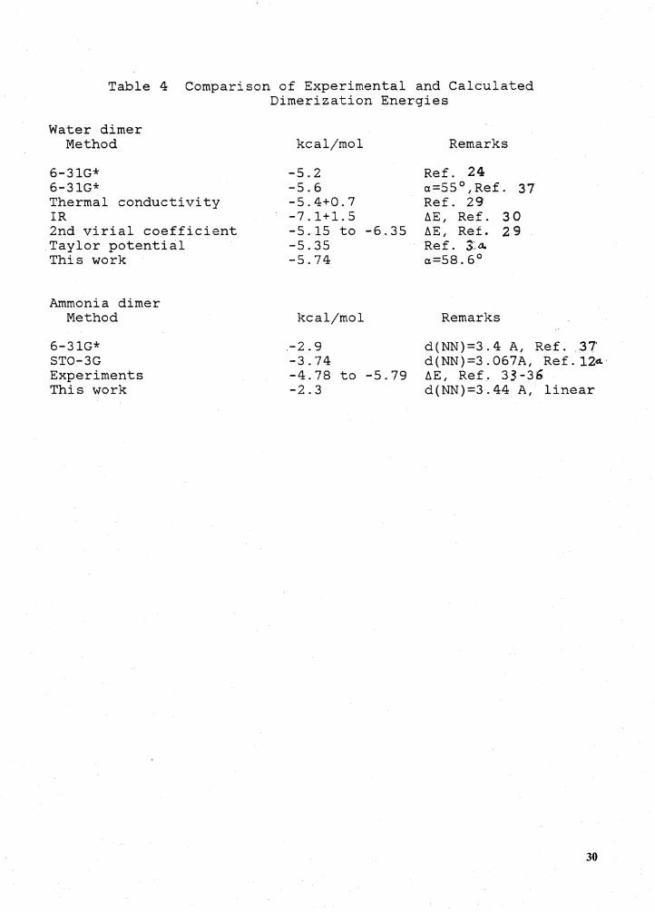
Table 4 Comparison of Experimental and Calculated Dimerization Energies
Water dimer Method
6-31G* 6-31G* Thermal conductivity IR 2nd virial coefficient Taylor potential This work
Ammonia dimer Method
6-31G* ST0-3G Experiments This work
kcal/mol
-5.2 -5.6 -5.4+0.7 -7.l+l.5 -5.15 to -6.35 -5.35 -5.74
kcal/mol
.-2. 9 -3.74 -4.78 to -5.79 -2.3
Remarks
Ref. 24 c:t=55°,Ref. 37 Ref. 29 ~E, Ref. 3 0 ~E, Ref. 2 9 Ref. 3,.a. a.=58.6°
Remarks
d(NN)=3. 4 A, Ref. .. 37' d(NN)=3.067A, Ref. 124 ~E, Ref. 33-36 d(NN)=3.44 A, linear
30
6-31G* basis was used. Using a ST0-3G basis set, Jorgensen et al. obtained -3.74 kcal/mol for a
slightly bent hydrogen bond with d(N-N)= 3.067 A. 12a.
Semiempirical and empirical results reported are -3.2 kcal/mo! for a constrained linear ammonia
dimer, -2.47 kcal/mol for an eclipsed near-linear dimer, -2.45 kcal/mol for a staggered linear dimer
and -2.27 kcal/mol for a closed cyclic dimer. 38
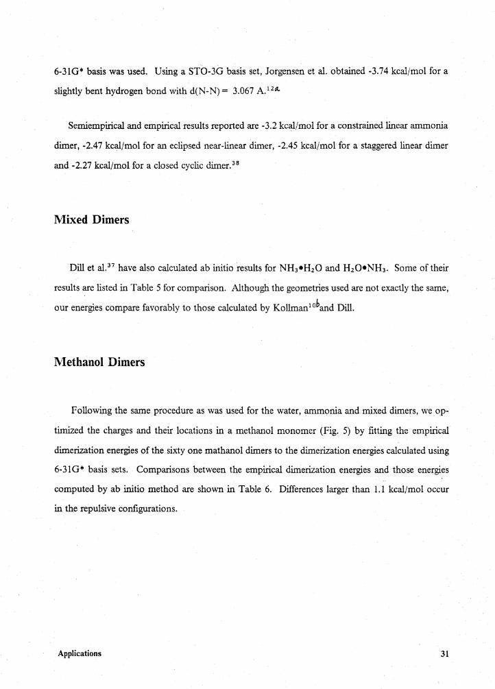
Mixed Dimers
Dill et al. 37 have also calculated ab initio results for NH3•H2 0 and H20•NH3 • Some of their
results are listed in Table S for comparison. Although the geometries used are not exactly the same,
our energies compare favorably to those calculated by Kollman10band Dill.
Methanol Dimers
Following the same procedure as was used for the water, ammonia and mixed dimers, we op-
timized the charges and their locations in a methanol monomer (Fig. 5) by fitting the empirical
dimerization energies of the sixty one mathanol dimers to the dimerization energies calculated using
6-31 G+ basis sets. Comparisons between the empirical dimerization energies and those energies
computed by ab initio method are shown in Table 6. Differences larger than 1.1 kcal/mol occur
in the repulsive configurations.
Applications 31
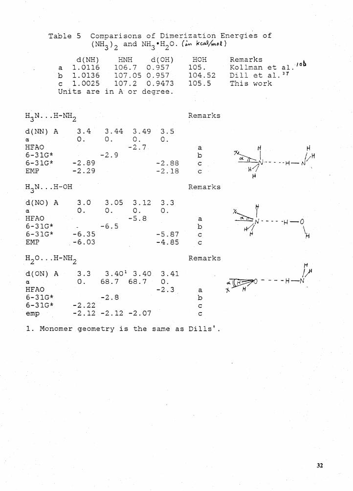
Table 5 Comoarisons of Dimerization Energies of (NH;) 2 and NH3 • H20. (;,..,, l<~/mo.e)
d(NH) HNH d(OH) a 1.0116 106.7 0.957 b 1.0136 107.05 0.957 c 1.0025 107.2 0.9473 Units are in A or degree.
H3N ... H-NH2
d(NN) A 3.4 a. 0. HFAO 6-31G* 6-31G* EMP
-2.89 -2.29
3.44 0.
-2.9
3.49 0.
-2.7
3.5 0.
-2.88 -2.18
H3N ... H-OH
d(NO) A 3.0 3.05 3.12 3.3
HFAO 6-31G* 6-31G* EMP
0. 0. 0. 0. -5.8
-6.5 -6.35 -5.87 -6.03 -4.85
H2 o ... H-NH2
d(ON) A 3.3 3.40 1 3.40 o; 0. 68.7 68.7 HFAO 6-31G* 6-31G* emp
-2.8 -2.22 -2.12 -2.12 -2.07
3.41 0.
-2.3
HOH 105. 104.52 105.5
Remarks
a b c c
Remarks
a b c c
Remarks
Remarks Kollman et al. icb Dill et al. 31 This work
x H.I
~ . -r,J- - - - -µ-o H/,! \
H H
rt /~ c1.JE?O - - - -H-N
a 1- H . b c c
1, Monomer geometry is the same as Dills'.
32
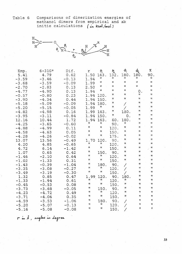
Table 6
Emp. 5.41
-3.59 -3.68 -2.70 -4.77 -0.57 -3.90 -5.18 -5.20 -4.82 -3.95 12.16 -4.25 -4.88 -4.58 -4.28 13.07 4.20 4.72 1. 07
-1.46 -1.02 -1.43 -3.35 -3.49 1. 32
-1. 33 -0.45 -3.73 -4.23 -3.71 -4.59 -5.20 -5.16
• r ~A,
Comparisons of dimerization energies of methanol dimers from empirical and ab ini tio calculations ( i., ke&J/fflol)
6-31G* Dif. r e; ~ q,I
4.79 0.62 1. 50 163. 132. 180. -3.46 -0.13 1. 94 " It fl
-3.59 -0.09 1. 99 It " " -2.83 0.13 2.50 " II " -4.90 0.13 1. 94 It fl !I
-0.80 0.23 1. 94 120. It It
-4. 34 0.44 1. 94 150. I! It
-5.09 -0.09 1. 94 180. " I -5.15 -0.05 1. 99 II II I -4.98 0.16 1. 99 163. " 180. -3.11 -0.84 1. 94 150. II 0. 10.44 1. 72 1. 94 163. 60. 180. -3.65 -0.60 II II 90. ll
-4.99 0.11 II " 120. II
-4.63 0.05 " " 150. " -4.26 -0.02 " " 175. " 13.56 -0.49 1. 70 120. 90. II
4.85 -0.65 It " 120. " 6.14 -1.42 " " 150. II
0.65 0.42 II 150. 90. II
-2.10 0.64 " " 120. " -1. 33 0.31 " " 150. " -0.39 -1.04 II 180. 90. I -3.08 -0.27 It It 120. I -3.19 -0.30· It " 150. I 0.85 0.47 1. 99 120. 90. 180.
-1.94 0.61 " " 120. " -0.53 0.08 " II 150. " -3.68 -0.05 " 150. 90. II
-4.72 0.49 II It 120. It
-4.06 0. 35 " " 150. il
-3.53 -1. 06 " 180. 90. I -5.07 -0.13 " " 120. I -5.08 -0.08 It " 150. I
°"'"1k..s ;,,.. le.( ret..
<t>,. x 180. 90.
It It
II It
" It
0. " It I!
II II
It " II II
It II
II " " II
II " " It
" II
It " " " It " " It
It " It II
fl It
II " II " " " It " II " " " !I II
'' !I
It It
" " " " It "
33
Table 6 Comparisons of dimerization energies of methanol dimers from empirical and ab initio calculations (continued)
Emp. 6-31G* Dif. r e; ~ 4', q,z. x. -2.60 -3.16 0.56 2.50 120. 90. 180. 0. 90. -2.14 -2.90 0.76 II II 120. " II II
-1. 38 -1. 89 0.51 II II 150. " II " -3.67 -3.52 -0.15 " 150. 90. II II II
-3.32 -3.70 0.38 II II 120. II 1! fl
-2.93 -3.29 0.36 " II 150. II II It
-3.72 -3.05 -0.67 " 180. 90. I " II
-3.74 -3.83 0.09 " II 120. I II " -3.67 -3.83 0.16 II fl 150. I II " -2.08 -2.24 0.16 3.00 120. 90. 180. If " -1.40 -1.70 0.30 II II 120. II " " -0.87 -1. 09 0.22 II II 150. II II II
-2.36 -2.03 -0.33 II 150. 90. II II II
-2.06 -2.17 0.11 II II 120. !I II " -1. 80 -1. 96 0.16 II II 150. 11 II " -2.30 -1. 69 -0.61 II 180. 90. I II fl
-2.30 -2.26 -0.04 II II 120. I II 11
-2.26 -2.31 0.05 It II 150. I II II
-0.89 -0.52 -0.37 4.00 120. 90. 180. II !I
-0.55 -0.29 -0.26 " II 120. II II II
-0.28 -0.04 -0.24 II II 150. fl II " -0.96 -0.39 -0.57 II 150. 90. II II !I
-0.85 -0.49 -0.36 II " 120. II " fl
-0.73 -0.44 -0.29 II II 150. II II II
-0.91 -0.26 -0.65 " 180. 90. I II " -0.96 -0.54 -0.42 II II 120. I " II
-0.96 -0.62 -0.34 II " 150. I II II
34

Water oligonzers
Non-cyclic trimers (H20)3
We computed stabilization energies of five non-cyclic trimer configurations39 (Fig. 7), using our
empirical potential with d(OH) = 0.9572 A, HOH= 104.52 degree. The results are listed in Table
7. Taylor3 a. and Newton et al 39 calculated the energies of those configurations with an empirical
potential and ab initio 4-31 G calculations respectively. We recalculated the 4-31 G values:
VABC = Er - 3Emon = r V(2) + v(3) . These are listed in Table 7 to illustrate the basis set depend-
ence. The difference in the values between each VABc of the ab initio result and the corresponding
r V<2l of our potential result are the sums of nonadditive energies and the errors; these are related
to the basis set chosen as reference. Our empirical parameters were obtained by fitting to 6-31G"'
calculated energies, so disagreement with the 4-31G calculations is not surprising.
Applications 35
Cyclic (H2Q)3 with C3 symmetry
The configurations used are shown in Fig. 8 and are the same as those used by Lentz et al .. 25
The results from our empirical potential and from 6-31G"' calculations, as well as those from
Lentz25 are listed in Table 8 for comparison. The monomer geometry is the same as that adopted
by Lentz: d(OH)=0.9450 A and HOH= 106 degree.
Since the optimized parameters were computed by consideration of pairwise interactions, no
estimate of non-additive interactions were obtained. Non additive corrections, V<nl, where n is equal
to or larger than 3, were estimated for water oligomers on the basis of Lentzs' ab initio results. 2 5
The three body non-additive energy, V<3l, is calculated using the relationship:
v(3) = ET - 3Emon - 3 V(2), where v(2) is the dimerization energy of an isolated pair. The differences
between our total pairwise potential 3 V(2l and Lentzs' total pairwise 3 V<2l are as large as 6.22
kcal/mol. However, the differences between 3 Vi2l calculated using our potential and the 6-31 G*
results are less than 3.2 kcal/mol. Since the optimized parameters of the new potential are based
primarily on 6-31G+ calculations (Of the 216 configurations 155 configurations were calculated with
the 6-31G* basis set.), it is more reasonable to compare the empirical potential results with those
computed using the 6-31G+ basis. The differences between 3V<2l from our 6-31G* ab initio calcu-
lations and those computed by Lentz are from 2.1 to 3 kcal/mol. These differences arise from the
use of different basis sets and causes the empirical potential results to differ from that of Lentz by
as much as 6 kcal/mol. However, the values of V<3l from our 6-31G* and Lentz' basis set differ
by less than 0.2 kcal/mol. This indicates that, in the treatment of ice-h, it should be satisfactory to
use Lentz's non-additive terms.
Applications 36
Table 7 Results for non-cyclic (H2o) 3 ( ~ k~/imol)
New Paten.a
1. 2. 3. 4. 5.
v<2)
-5.30 -4.62 -6.14 -5.02 -4.63
a. This work. b. VABC=ET-JEmon
Configuration r(Hl-01), A r(Hl-02), A r(Hl-03), A
HOlHl,deg 81, deg 82, deg 81 ! I deg 83, deg ¢1, deg ¢2, deg ¢3, deg x2, deg x3, deg
1 .9572 2.15 2.15 104.52 135. 132. 135. 132. 180.
0, 180.
90. 90.
VABC -6.26 -5.63 -6.80 -5.51 -5.03
2 .9572 2.15 2.15 104.52 135. 132. 135. 132. 180.
0. 90. 90. 90.
6-31G*a
Dif.
-0.96 -1. 01 -0.66 -0.49 -0.40
3 .9572 1. 95 2.50 104.52 150. 132. 110. 132. 180.
0. 180.
90. 90.
VABC -10.26
Dif.
-4.96 -8.85 -4.23
-10.96 -4.82 -9.10 -4.08 -7.89 -3.26
4 .9572 1. 95 2.50 104.52 150. 132. 110. 132. 180.
0. 90. 90. 90.
5 .9572 1. 95 2.50 104.52 150. 132. 110. 132. 180.
0. 0.
90. 90.
37
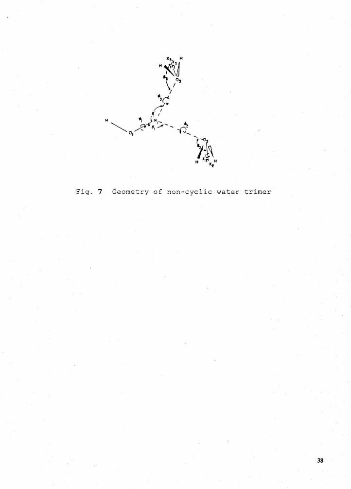
Fig. 7 Geometry of non-cyclic water trimer
38
Table 8 Results for C3 cyclic (H20) 3 (~" ke.J./mol)
R(OO) A
2.56 2.81 3.00 3.25
R(OO) A
2.56 2.81 3.00 3.25
Our Poten. 2.42
-7.47 -8.48 -7.29
a This work. b Reference 2 5".
6-31G*a 3V( 2 ) Dif. 5.61 3.19
-5.75 1.72 -7.95 0.53 -7.76 -0.47
VABC 2.13
-7.17 -8.74 -8.18
6-31G*a v ( 3)
-3.48 -1.42 -0.79 -0.42
b Lentz 3V( 2 ) 8.64
-2.73 -5.34 -5.64
Dif. 6.22 4.74 3.14 1. 65
Lentzb
VABC 4. 98
-4.24 -6.18 -6.10
v<3) -3.66 -1. 51 -0.84 -0.46
39
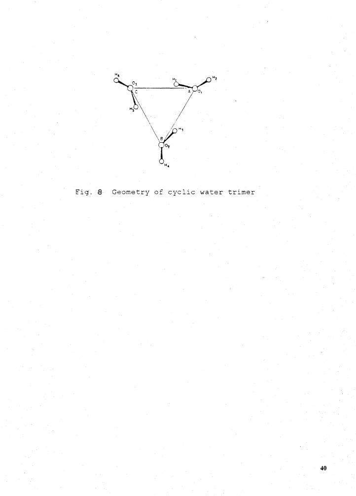
Fig. 8 Geometry of cyclic water trimer
40
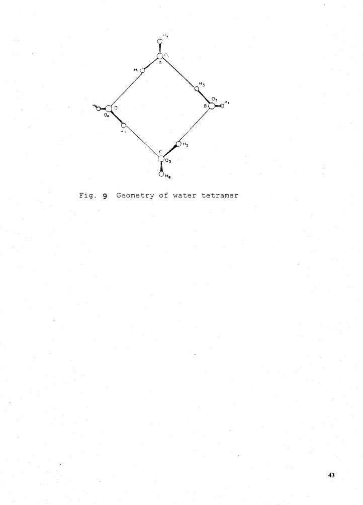
Cyclic (H2 0 )4 with S4 symmetry
I v(2) = 4 v~21 + 2 v~2b. I
where V\'), ~ E,. -2£.," and V\'t ~ E,c -12Emon
V(3l = E - 2£(21 - £(21 ABC .·AB AC
where Vi21 or Vfib is the dimerization ener9 of the isolated pair AB or AC.
I
As seen in Table 9, the differences betv..len the total V(2l computed from the empirical potential
and from the 6-31G* basis areless than 3 Jcal/mol. In Tables 8 and 9 the pairwise empirical po-
tential energies are shown to deviate from tbe results of 6-31G* by around 3 kcal/mol. This is the
result of accumulated errors. For the dimJr, the error is only about 0.5 kcal/mol. Since the total I
pairwise energy for an S4 tetramer in the ~otential calculation is composed of four pairwise AB I I
energy values and two pairwise AC energ~ values (see Figure 9), the accumulated error could be I
as high as 3 kcal/mol. The small differenqes between V(3l and V<4> of the 6-31G+ basis and those I I
of Lentz again suggests it is reasonable to estimate non-additive energies directly from Lentzs' data.
Applications 41
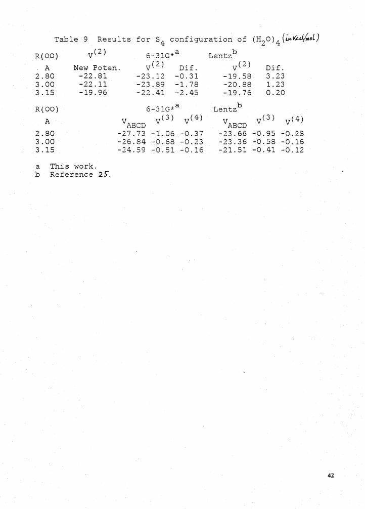
Table 9 Results for S 4 configuration of (H2o) 4 (U.t<4ol)
R(OO) . A 2.80 3.00 3.15
R(OO) A
2.80 3.00 3.15
a This
New Paten . -22.81
6-31G*a v<2)
-23.12 Dif.
-0.31 -22.11 -23.89 -1.78 -19.96 -22.41 -2.45
6-31G*a
VABCD v(3) v<4)
-27.73 -1. 06 -0.37 -26.84 -0.68 -0.23 -24.59 -0.51 -0.16
work. b Reference 25".
b Lentz v<2)
-19.58 -20.88 -19.76
Lentz b
VABCD -23.66 -23.36 -21.51
Dif. 3.23 1. 23 0.20
v( 3) v<4)
-0.95 -0.28 -0.58 -0.16 -0.41 -0.12
42
...
... '!
Fig. 9 Geometry of water tetramer
43
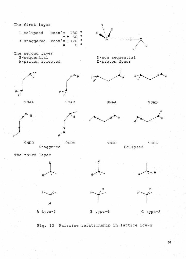
Ice-h
The lattice energy of ice-h has been estimated from experimental data to be -13.4 kcal/mol2°.
In ice-h, each oxygen is surrounded by four oxygen atoms in the first neighbouring layer. The four
oxygen atoms are oriented in a near tetrahedral configuration. Each H2 0 makes four H-bonds with
the nearest oxygen atoms; two protons comes from the central oxygen and the other two protons
from neighbouring H2 Os. Pauling40 1 41 hypothesized the six possible combinations have equal
probability. The lattice energy of ice-his calculated on the basis of this hypothesis. The H-bonding
energy of ice-h can be defined as one half of the lattice energy of a mole of ice. This is one of several
H-bonding definitions22 for ice.
The space group of ice-h is D~ -C6/mmc.41 From the neutron diffraction of 0 2 0,
d(O-D) = 1.01 A. d(0-0) = 2.76 A and the angle among any three neighbouring oxygen atoms are
109.63 degree if two of the three oxygens are along the crystal c axis and 109.31 degree if no two
oxygen atoms are along the c axis. 2° From proton magnetic resonance studies, d(H-H)= 1.584
A.42 For simplicity, we have adopted regular tetrahedral configurations for the empirical calcu-
lations. We used d(0-0) = 2.76 A and d(O-H) = 1.0 A in our calculations.
The lattice surrounding an arbitrary oxygen atom has the following structure: The four oxygens
in the first layer are at a distance of d(0-0) = 2.76 A from the central oxygen. In the second layer
Ice-h 44

there are twelve oxygens with d(0-0) = 4.51 A; three above the central oxygen along the c axis, and
three below. The remaining six and the central oxygen are in a plane perpendicular to the c axis.
Only one oxygen with d(0-0) = 4.60 A is in the third layer. Because the values of d(0-0) for the
second and the third layers are similar, Lentz et al. included the single H20 of the third layer as a
part of the second layer. Interactions from the fourth layer and beyond are neglected both in our
calculations as well as those of Lentz ei al ..
First Layer Lattice Energy
The H20 along c in the first layer has its hydrogens eclipsed with those of the central H20.
The remaining H20s have staggered hydrogen configurations. There are three eclipsed configura-
tions for the oxygen along the c axis. Each of the other three oxygens has three staggered config-
urations. Therefore, there are a total of three eclipsed and nine staggered configurations. In
accordance with Pauling's hypothesis, we assumed that each of the twelve configurations occurs
with the same probability. Using Pauling's hypothesis to determine the weighting factors, the av-
erage V~21 for the first layer is -5.11 kcal/mol in the empirical calculation. The total first layer lattice
energy, which is one half of the 4• v')l1 interactions, is -10.23 kcal/mol.
Calculations were also carried out for this layer using the 6-31G+ basis set for comparison. The
result is -4.49 kcal/mol for the average V~1, i.e. -9.0 kcal/mol for the total first layer lattice energy.
For the first layer energy, the 6-31G* results (this work), the empirical results (this work) and
the results of Ben-Nairn Stillinger potential5 are listed in Table 10. The empirical result (-10.l
kcal/mol) is much lower than Lentzs' value (-6.5 kcal/mol) and should be higher than that calcu-
lated from Ben-Nairn Stillinger's potential. However, it is close to the results calculated using a
6-31 G + basis set.
Ice-h 45
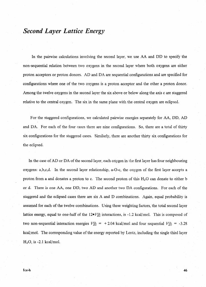
Second Layer Lattice Energy
In the pairwise calculations involving the second layer, we use AA and DD to specify the
non-sequential relation between two oxygens in the second layer where both oxygens are either
proton acceptors or proton donors. AD and DA are sequential configurations and are specified for
configurations where one of the two oxygens is a proton acceptor and the other a proton donor.
Among the twelve oxygens in the second layer the six above or below along the axis care staggered
relative to the central oxygen. The six in the same plane with the central oxygen are eclipsed.
For the staggered configurations, we calculated pairwise energies separately for AA, DD, AD
and DA. For each of the four cases there are nine configurations. So, there are a total of thirty
six configurations for the staggered cases. Similarly, there are another thirty six configurations for
the eclipsed.
In the case of AD or DA of the second layer, each oxygen in the first layer has four neighbouring
oxygens: a,b,c,d. In the second layer relationship, a-0-c, the oxygen of the first layer accepts a
proton from a and donates a proton to c. The second proton of this I-IzO can donate to either b
or d. There is one AA, one DD, two AD and another two DA configurations. For each of the
staggered and the eclipsed cases there are six A and D combinations. Again, equal probability is
assumed for each of the twelve combinations. Using these weighting factors, the total second layer
lattice energy, equal to one-half of the 12• V12t interactions, is -1.2 kcal/mol. This is composed of
two non-sequential interaction energies V12t = + 2.04 kcal/mol and four sequential V)[b = -3.28
kcal/mol. The corresponding value of the energy reported by Lentz, including the single third layer
I-120, is -2.l kcal/mol.
46
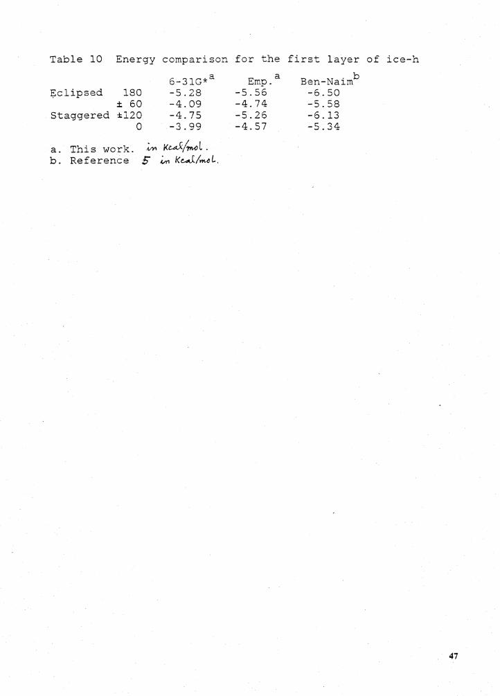
Table 10 Energy comparison for the first layer of ice-h
:i;::clipsed 180 ± 60
Staggered ±120 0
6-31G*a -5.28 -4.09 -4.75
. -3. 99
a. This work. ~ 1<e.tX/""'°L . b. Reference S .i,.,, kw/>ML.
Emp. -5.56 -4.74 -5.26 -4.57
a Ben-Naimb -6.50 -5.58 -6.13 -5.34
47
Third Layer Lattice Energy
Only one oxygen atom is in the third layer, 4.60 A from the central oxygen atom. Although
there are 6 distributional possibilities for each pair of protons belonging to an oxygen located in the
center of a tetrahedron and 36 possibilities for such a pair of oxygen atoms in the third layer, once
the water dimer is isolated from the crystal, twelve configurations suffice to describe the interactions.
Using weighting factors based on the above arguments, we computed V)lb to be + 0.026 kcal/mol.
The third layer lattice energy contrubution is one half of this value: + 0.013 kcal/mol.
The lattice energy of ice-h approximated to the third layer as expressed by Lentz et al. 25 is:
£ice = 2( V121)a• + 4( V~t + V131c)a,,eq + 2( V:ft + V~1c)a•nonseq + 2 V2B + 6 V2c·
The results calculated from our empirical potential and Lentzs' ab initio results25 are listed in
Table 11. The non-additivity contributions, taken directly from Lentz et al., is -4.36 kcal/mol. The
lattice energy of ice-h calculated from our empirical potential using Lentzs' value for the non-
additivity contributions is -15.6 kcal/mol. Lentzs' result is -12.9 kcal/mol. These calculated results
bracket the estimated experimental value of -13.4 kcal/mol. 22 In contrast, the lattice energy calcu-
lated using CND0/2 is -4.9 kcal/mol.43
lce-h 48
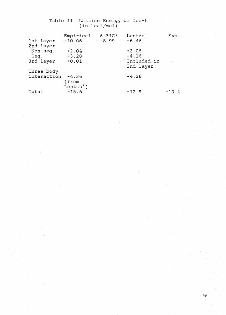
Table 11 Lattice Energy of Ice-h (in kcal/mol)
Empirical 6-31G* Lentzs' Exp. 1st layer -10.06 -8.99 -6.46 2nd layer
Non seq. +2.04 +2.06 Seq. -3.28 -4.16
3rd layer +0.01 · Included in 2nd layer.
Three body interaction -4.36 -4. 36
(from Lentzs')
Total -15.6 -12.9 -13.4
49
The first layer
1 eclipsed xoox'= 180 ° = ± 60 °
3 staggered xoox' = ± 120 ° = 0 0
The second layer s-sequential A-proton accepted
~rl r J ~-t H H
9NAA 9SAD
(H (" ~/ ~/
9NDD 9SDA Staggered
The third layer
H J_
A type-3
'i.
H~/ . 0 - - - - - - -H-O
I '\ .. :-1
x'
N-non sequential D-proton doner
9NAA
9NDD Eclipsed
9SAD
9SDA
B type-6 C type-3
Fig. 10 Pairwise relationship in lattice ice-h
50
Methanol crystal, 13-modification
An IR study of the shift of the 0-H vibration frequency44 led to an estimate of -7.5 kcal/mol
for the strength of the hydrogen bonds in methanol.
We applied our pairwise empirical potential to the 13 modification of methanol and calculated
a value of -7.9 kcal/mol for the lattice energy. Only pairwise relationships among the monomers
in the crystal were considered. The cut-off lengths are tak:en to be the same as the parameter a of
the orthorombic unit cell. To obtain the appropriate distances, we made use of the coordinates of
the carbons ~d oxygens based on the results of X-ray diffraction.45 The coordinates of hydrogen
atoms were based on our optimization result of a 6-31G* basis calculation of the methanol
monomer. Their cartesian coordinates in Angstrom are listed in the Appendix A. Listed below
are the five kinds of pairwise interactions considered:
E(AB) = -2.13 kcal/mol x( 1/2) x 2 neighbors
E(AB') = -1.11 kcal/mol x(l/2) x 2 neighbors
E(AG) = -1.48 kcal/mo! x(l/2) x 4 neighbors
E(AD) = -0.84 kcal/mol x(l/2) x 2 neighbors
E(AD') = -0.84 kcal/mol x( 1/2) x 2 neighbors
Methanol crystal, j)-modification 51
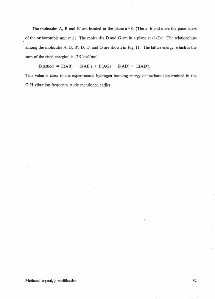
The molecules A, B and B' are located in the plane a= 0. (The a, band care the parameters
of the orthorombic unit cell.) The molecules D and Gare in a plane at (l/2)a. The relationships
among the molecules A, B, B', D, D' and Gare shown in Fig. 11. The lattice energy, which is the
sum of the cited energies, is -7.9 kcal/mol.
E(lattice) = E(AB) + E(AB') + E(AG) + E(AD) + E(AD').
This value is close to the experimental hydrogen bonding energy of methanol determined in the
0-H vibration frequency study mentioned earlier.
Methanol crystal, P-modification 52
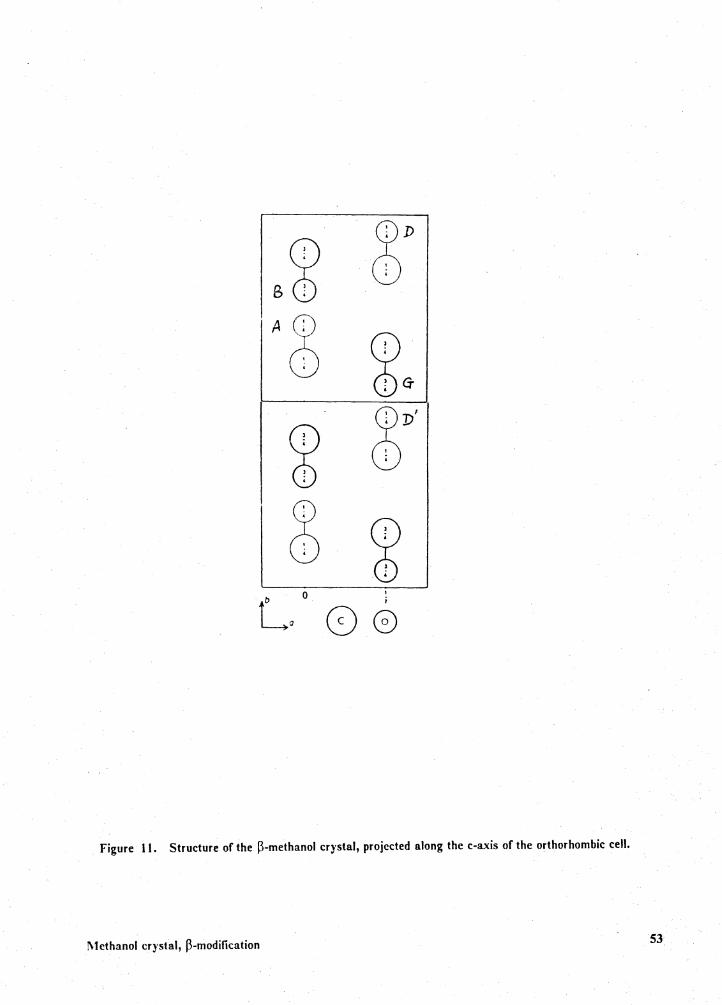
·~· 8D'
8 ~ ' r
80
Figure 11. Structure of the P-methanol crystal, projected along the c-axis of the orthorhombic cell.
Methanol crystal, P-modilitation

Conclusion
1. The empirical potential used in this thesis is composed of two parts: electrostatic interactions
and van der Waals interactions. The van der Waals interactions are the same as those used in
Allinger's molecular mechanics program, MM2.18 ~ Point charges models were used for the
electrostatic interactions. The parameters of the point charge models were optimized through a
simplex optimization program to fit the empirical results to ab initio results (6-31G* basis set and
MCYs' CI calculations). Neither Morse terms nor the orientations of the dipoles were involved in
our empirical potential. Therefore, our potential is simpler than Taylor's3a.and Kroon's4, which
do use these terms in their potentials.
2. Comparison of the results of the empirical potential, the experimental results· and those of
6-31G* ab initio calculations for several cases of water oligomers, ice-h and the ammonia dimer
showed that the differences are ca. 1 kcal/mol for the various dimerization energies. The empirical
potential can be applied to calculate reasonable pairwise stability energies of water oligomers and
ammonia dimers.
3. The results from the empirical potential are comparable to those from 6-31 G* calculations.
When compared to the results of other basis sets, the differences between the results of 6-31G* and
Conclusion 54
those of the other basis set must be taken into account. The empirical potential is for interactions
of pairs of monomers and non-additive interaction energies are not computed.
4. The potential is compatible with the MM2 program.
5. The local H-bonding energies of a large molecule t:an be estimated with the empirical po-
tentials. Extensions should be applicable to consideration of H-bonding in carbohydrates and
polypeptides.
Conclusion 55
Determination of the Orientation of Anthracene
Molecules in the Unit Cell by means of a
Refractivity Method
Determination of the Orientation of Anthracene Molecules in the Unit Cell by means of a Refractivity Method 56
Introduction
The dependence of a crystal's refractive indices on the structure and orientation of its constituent
molecules has been exploited in several different ways. Bragg46'2; 46 hand Zachariasen47 calculated
the refractive indices of calcite, aragonite and sodium bicarbonate crystals from their atomic ar-
rangements. On the basis of the birefringence in calcite and sodium nitrate crystals, Bragg46b de-
termined the bond distance for N-0. Bhagavantam48 ~ 48 b determined the magnetic and optical
properties of aromatic compounds and attempted to relate the properties to the orientation of the
molecules in the crystal lattice. For anthracene, using the molecular structure and its orientation
from X-ray diffraction, Julian and Bloss49 calculated the molecular refractivities from the refractive
indices of the crystal. Bunn50 calculated its crystal refractive indices from the directional bond
polarizabilities of the molecular bonds. The purpose of the present study is to illustrate the reverse
procedure; we investigate the possibility of determining the molecular orientation in the unit cell
by matching the macroscopic optical properties of the crystal to those calculated from a molecular
structure.
The macroscopic directional refractivities of the crystal, the density, the point/space group of
the crystal and the crystal constants as well as the molecular structure are assumed to be known.
Starting with empirical bond polarizabilities, we use the simplex method to optimize the molecular
orientation by matching the orientation and shape of the crystal refractivity ellipsoid. While our
Introduction 57

calculation is confined to anthracene, the idea can be extended to any other monoclinic crystal
without difficulty. In fact, except for the cubic system with isotropic properties, this method should
also be capable of extension to other crystal systems.
Introduction 58
Method
To illustrate the method we use an approximate molecular geometry for anthracene in which
the aromatic rings are assumed to be regular hexagons, and all bond angles are taken to be 120°.
Figure 12 shows the idealized molecular geometry and indicates the directions (l,m,n) of the prin-
cipal components of its polarizability tensor. We employ the standard longitudinal (P1) and trans-
verse (P1) bond polarizabilities listed in Table 12 and calculate the three principal components of
molecular polarizability by summing over all bonds, b:
(1)
where Ab; is the angle between the bth bond and the ith axis. The principal molar refractivities are
then calculated from
ru = (4n/3)Npi,(i = l,m,n) (2)
where N is Avogadro's number. The values obtained for anthracene are:
ru = 76.4cc/mole rmm = 69.7cc/mole rnn = 34.Scc/mole.
Method 59
To describe the crystal refractivities, we use an orthogonal coordinate system (a',b',c'), where
a' and b' are chosen parallel to the crystal axes a and b, and c' is taken to be perpendicular to a'
and b'. For simplicity, (a,b,c') is used to express (a',b',c'). If we use ujk to represent the direction
cosine of unit vector j with respect to the direction k, and note that ujk = ukj , we can use the fol-
lowing orthogonal transformation to transform the molecular refractivities to the (a,b,c') coordinate
system:
[ u,, Uam Uan H 0 0
r~ U\b U[c' l R = Ubl Ubm Ubn rmm 0 Uma Umb Umc' (3) ' 0 Uc'/ U'· Uc•n rnn Una Unb Unc' cm
The anthracene crystal has symmetry P21 /a. The two molecules in the unit cell differ in ori-
entation only with respect to the signs of u1b , um6 and u,,,;; the magnitudes of these as well as the
magnitudes and signs of the other direction cosines are identical for the two molecules. When one
averages the result of equation (3) for the two molecules in the unit cell the following is obtained
for the molar refractivity of the crystal:
(4)
whei:e j = 1,m,n. The four zeroes arise from the sign changes in !lib , umb and u,,,; noted earlier. The
form of this matrix is typical of second order tenso.r properties for monoclinic crystals (Sands51 ).
Diagonalization of this matrix yields three principal refractivities as the eigenvalues. The direction
cosines of the principal axes relative to a, b, and c' are obtained from the eigenvectors. The calcu-
lated matrix has a trace of 180.60, while the sum of the three principal refractivities from experiment
(Julian and Bloss49 ) is 187.97. The difference between these numbers reflects errors in the a9-
proximate molecular structure and in the empirical bond polarizabilities employed. This slight error
will make exact predictions of molecular orientations impossible.
Method 60
For each set of assumed molecular orientations a corresponding resultant ellipsoid can thus be
calculated. For the monoclinic crystal the orientation of this ellipsoid in three dimensional space
is described by an angle between c' and the longest principal axis. The difference between the ex-
perimental and the calculated angles can be used as one standard for optimization of the molecular .
orientation in the unit cell. For anthracene P= 124.7°, U=7.5° (the angle between the longest
principal semi-axis and the monoclinic c), so the experimental angle from c' is 27.2°. In addition
we can compare the shapes of the calculated and experimental ellipsoids as measured by the ratios
Rz/R1 and Ra/R1. Here R1 is the smallest eigenvalue and R2 is the largest. For anthracene the
ratios of the principal semi-axes of the experimental refractivity ellipsoid are Rz/R1 = 1.805 and
A linear combination of these standards with different weighting factors ( C;) yields a function
F which can be minimized to determine the correct molecular orientation:
(5)
~is the deviation between the experimental angle, 27.2°, and the calculated one.
Since the nine direction cosines for a molecule must satisfy the usual orthonormality conditions
(Nye52), only three out of the nine are independent. We chose u1a, Zlib and uma as the independent
parameters. These must satisfy the consistensy conditions:
and
to ensure that all direction cosines are real. For each choice of these three, we solved the
orthonormality equations for the remaining direction cosines and used equation (4) to obtain the
crystal refractivity tensor. Because of the quadratic nature of the orthonormality equations, this
Method 61

procedure gives eight different solutions, four of which refer to the orientation of each molecule in
the unit cell. The four solutions for each molecule are related to one another by a reflection
through the (a,b) plane and a second reflection through the (l,m) plane.
Method 62
Optimization of the Molecular Orientation
A simplex algoritlun (O'Neill 1 5) _was used to minimize F ( eq. ( 5)) with respect to the orientation
of the anthracene molecules. In practice we found that there are an infinite II.umber of ellipsoidal
orientations with zero~. which indicates that the orientation condition as reflected in~ is a weaker
condition and the first term of eq. (5) should receive relatively little weight. Best results were ob-
tained with C1 = 0.02 and C2 = C3 = 1.0.
Table 13 lists the three starting angle set and the optimized angle set for several calculations.
The errors between the actual orientation and the calculated orientation of anthracene molecule's
in the unit cell differ by less than 10°. The optimized angle sets with F less than or equal to 0.088
appear to represent reasonable results. For most starting sets chosen, initial step angles of 30° were
found to be suitable for optimization.
1bis method can be used for other monoclinic molecular crystals. It should also be possible
to apply this optimization method of molecular orientation to other crystal systems with the ex-
ception of the cubic system with isotropic molecular properties. It may also be useful in studies
of optical properties of liquid crystals.
Optimization of the Molecular Orientation 63
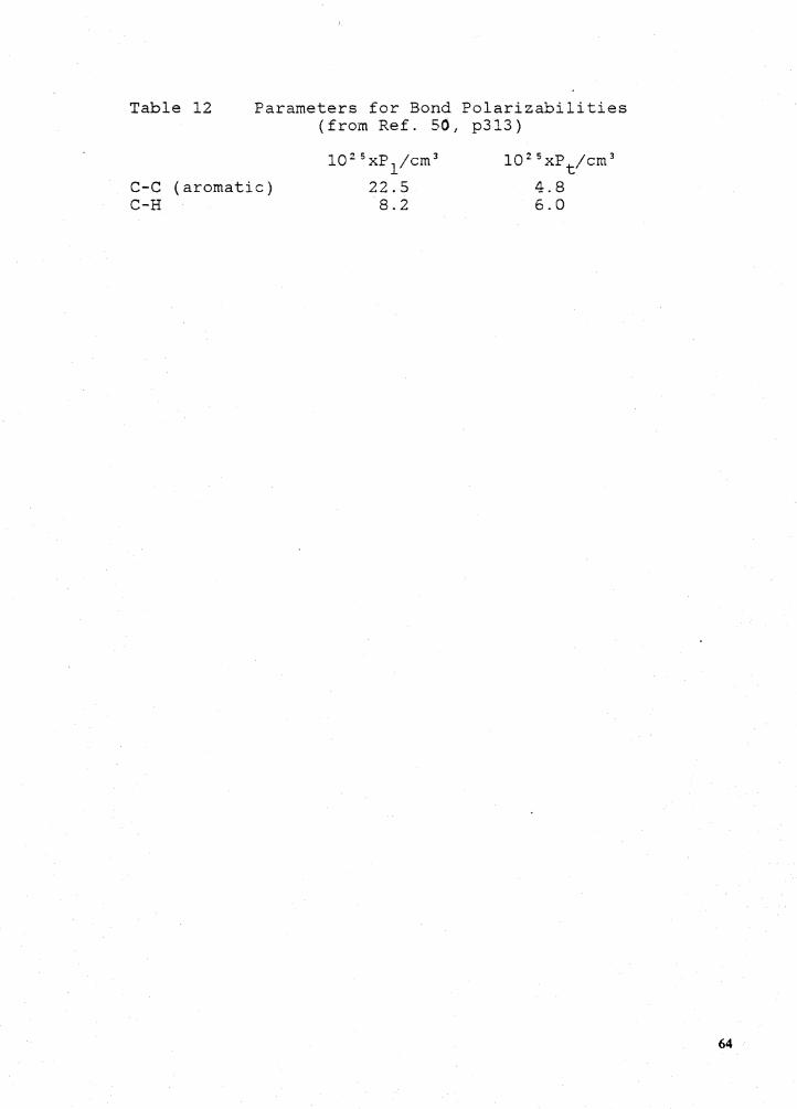
Table 12 Parameters for Bond Polarizabilities (from Ref. 50, p313)
C-C (aromatic) C-H
10 25 xP /cm 3 1
22.5 8.2
10 25 xP./cm 3 t
4.8 6.0
64
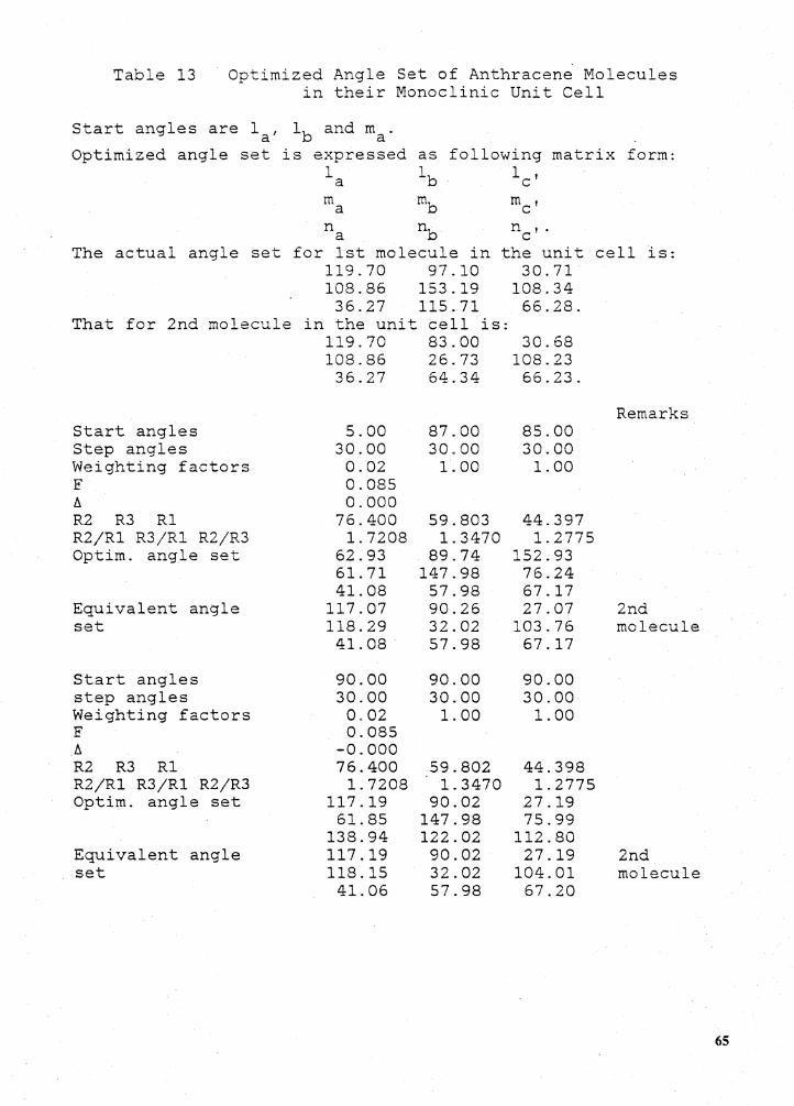
Table 13 Optimized Angle Set of Anthracene Molecules in their Monoclinic Unit Cell
Start angles are la, lb and ma. Optimized angle set is expressed as following matrix form:
la lb le' m mb m c' a n nb n c'. a
The actual angle set for 1st molecule in the unit cell is: 119.70 97.10 30.71 108.86 153. 19 108.34
36.27 115.71 66.28. That for 2nd molecule in the unit cell is:
119.70 83.00 30.68 108.86 26.73 108.23
36.27 64. 34 66.23.
Remarks Start angles 5.00 87.00 85.00 Step angles 30.00 30.00 30.00 Weighting factors 0.02 1. 00 1. 00 F 0.085 b,, 0.000 R2 R3 Rl 76.400 59.803 44. 397 R2/Rl R3/Rl R2/R3 1.7208 1. 3470 1.2775 Optim. angle set 62.93 89.74 152.93
61.71 147.98 76.24 41. 08 57.98 67.17
Equivalent angle 117.07 90.26 27.07 2nd set 118.29 32.02 103.76 molecule
41. 08 57.98 67.17
Start angles 90.00 90.00 90.00 step angles 30.00 30.00 30.00 Weighting factors 0.02 1. 00 1. 00 F 0.085 b,, -0.000 R2 R3 Rl 76.400 59.802 44.398 R2/Rl R3/Rl R2/R3 1.7208 1.3470 1.2775 Optim. angle set 117.19 90.02 27.19
61. 85 147.98 75.99 138.94 122.02 112.80
Equivalent angle 117.19 90.02 27.19 2nd set 118.15 32.02 104.01 molecule
41.06 57.98 67.20
65
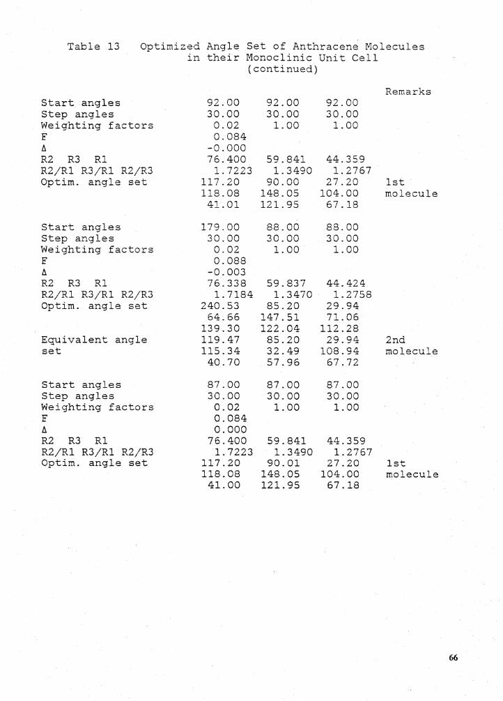
Table 13 Optimized Angle Set of Anthracene Molecules in their Monoclinic Unit Cell
(continued)
Remarks Start angles 92.00 92.00 92.00 Step angles 30.00 30.00 30.00 Weighting factors 0.02 1. 00 1. 00 F 0.084 A -0.000 R2 R3 Rl 76.400 59.841 44. 359 R2/Rl R3/Rl R2/R3 1.7223 1. 3490 1.2767 Optim. angle set 117.20 90.00 27.20 1st
118.08 148.05 104.00 molecule 41. 01 121. 95 67.18
Start angles 179.00 88.00 88.00 Step angles 30.00 30.00 30.00 Weighting factors 0.02 1. 00 1. 00 F 0.088 A -0.003 R2 R3 Rl 76.338 59.837 44.424 R2/Rl R3/Rl R2/R3 1. 7184 1. 3470 1.2758 Optim. angle set 240.53 85.20 29.94
64.66 147.51 71. 06 139.30 122.04 112.28
Equivalent angle 119.47 85.20 29.94 2nd set 115.34 32.49 108.94 molecule
40.70 57.96 67.72
Start angles 87.00 87.00 87.00 Step angles 30.00 30.00 30.00 Weighting factors 0.02 1. 00 1.00 F 0.084 A 0.000 R2 R3 Rl 76.400 59.841 44.359 R2/Rl R3/Rl R2/R3 1. 7223 1. 3490 1.2767 Optim. angle set 117.20 90.01 27.20 1st
118.08 148.05 104.00 molecule 41.00 121. 95 67.18
66
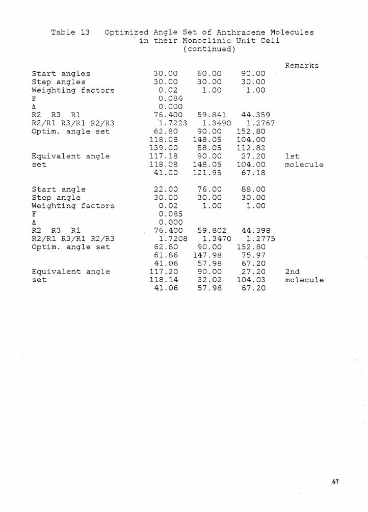
Table 13 Optimi.zed Angle Set of Anthracene Molecules in their Monoclinic Unit Cell
(continued)
Remarks Start angles 30.00 60.00 90.00 Step angles 30.00 30.00 30.00 Weighting factors 0.02 1.00 1.00 F ·0.084 f:. 0.000 R2 R3 Rl 76.400 59.841 44.359 R2/Rl R3/Rl R2/R3 1.7223 1. 3490 1.2767 Optim. angle set 62.80 90.00 152.80
118.08 148.05 104.00 139.00 58.05 112.82
Equivalent angle 117.18 90.00 27.20 1st set 118.08 148.05 104.00 molecule
41. 00 121.95 67.18
Start angle 22.00 76.00 88.00 Step angle 30.00 30.00 30.00 Weighting factors 0.02 1.00 1.00 F 0.085 6. 0.000 R2 R3 Rl 76.400 59.802 44. 398 R2/Rl R3/Rl R2/R3 1.7208 1.3470 1. 2775 Optim. angle set 62.80 90.00 152.80
61.86 147.98 75.97 41.06 57.98 67.20
Equivalent angle 117.20 90.00 27.20 2nd set· 118.14 32.02 104.03 molecule
41. 06 57.98 67.20
67
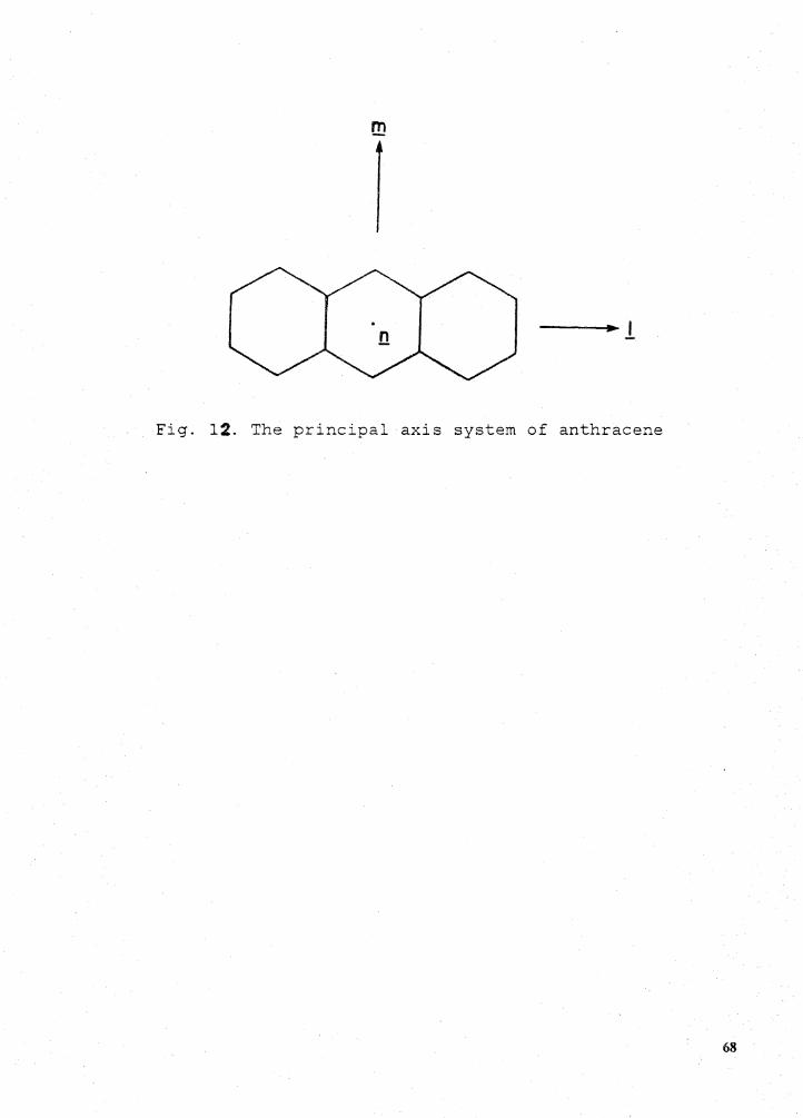
n
Fig. 12. The principal axis system of anthracene
68

Some Ab Initio Calculatio11s l11volvi11g The
Acetonitrile Exchange Reaction
Some Ab lnitio Calculations Involving The Acetonitrile Exchange Reaction 69
Introduction
Acetonitrile has been used as a solvent in reactions which introduce labelled carbon isotopes into
organic compounds. However, significant loss of the radioactivity of the products was found by
Jay et al. 6 This led them to postulate the following exchange reaction:
* * CH3CN + CN- = CH3CN + CN-.
A mixture of KCN labelled with carbon 13, normal acetonitrile and crown ether (18-crown-6) were
refluxed. When the distillate was analyzed with NMR and MS, they found an enrichment of
carbon-13 in the nitrile carbon of the acetonitrile.
They suggested that a mechanism involving addition-rearrangement-elimination processes,
scheme 1 in Fig. 13, was more likely than a SN2 mechanism (scheme 2, Fig. 13). Their reasoning
was that the cyanide anion is a good nucleophile but the cyano function is a poor leaving group in
the SN2 sense and nucleophiles such as hydroxide, alkoxides, amines and sodamide are known to
attach to the electrophilic carbon atom resulting in additions to the C = N bond rather than in
SN2 displacement of the cyano group. 53 Examples cited to support their arguments include: 1. A
Grinard reagent reaction with cyano functional group54 undergoes an addition rather than a dis-
placement, 2. Benzilic acid undergoes an analogous rearrangement55 a. and 3. The benzoin
condensation results in a loss of the cyanide ion. 5 5 a.
Introduction 70
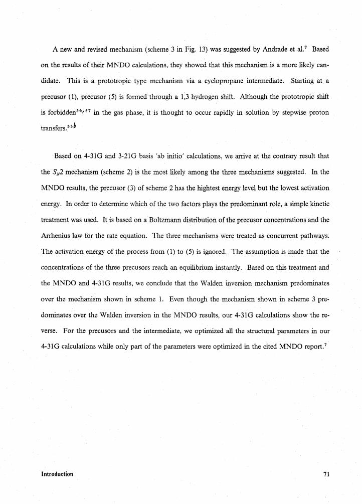
A new and revised mechanism (scheme 3 in Fig. 13) was suggested by Andrade et al.7 Based
on the results of their MNDO calculations, they showed that this mechanism is a more likely can-
didate. This is a prototropic type mechanism via a cyclopropane intermediate. Starting at a
precusor (1), pi:ecusor (5) is formed through a 1,3 hydrogen shift. Although the prototropic shift.
is forbidden56' 57 in the gas phase, it is thought to occur rapidly in solution by stepwise proton
transfers. 5 5 h
Based on 4-31G and 3-21G basis 'ab initio' calculations, we arrive at the contrary result that
the SN2 mechanism (scheme 2) is the most likely among the three mechanisms suggested. In the
MNDO results, the precusor (3) of scheme 2 has the hightest energy level but the lowest activation
· energy. In order to determine which of the two factors plays the predominant role, a simple kinetic
treatment was used. It is based on a Boltzmann distribution of the precusor concentrations and the
Arrhenius law for the rate equation. The three mechanisms were treated as concurrent pathways;
The activation energy of the process from ( 1) to ( 5) is ignored. The assumption is made that the
concentrations of the three precusors reach an equilibrium instantly. Based on this.treatment and
the MNDO and 4-31G results, we conclude that the Walden inversion mechanism predominates
over the mechanism shown in scheme l. Even though the mechanism shown in sche.me 3 pre-
dominates over the Walden inversion in the MNDO results, our 4-31G calculations show the re-
verse. For the precusors and the intermediate, we optimized all the structural parameters in our
4-31G calculations while only part of the parameters were optimized in the cited MNDO report.7
Introduction 71
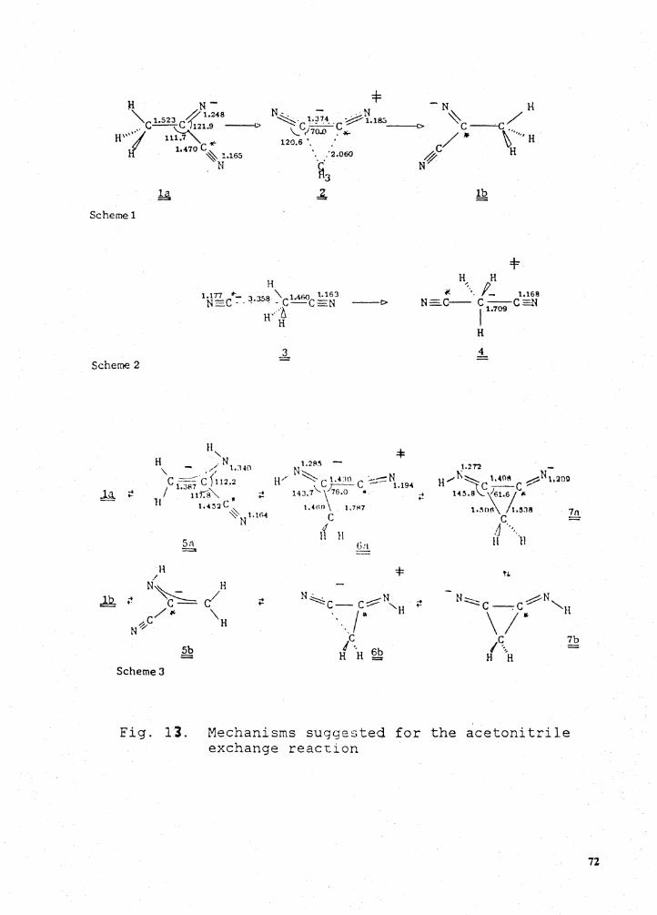
H N- -N H ., ~1.2-48 "c 1.s2J c -- 121.9 ---0
H'''/". 11~ N~ 1 374 ~N1 1°< ~ / ~c~c,...... ·~-c- ~c----c
\... '/10..0 . ..,.. / • ~· ..... , H
Scheme 1
Scheme 2
H /
1.470 c <(-
~ 1.165 N
1.177 .. _ N=C-
-+ N~ H •· c- r!
/~ \ -%C H N ,.-
Scheme 3
120.6 '. : ~ '. :2.oso 4-:C H ·~3 N .
.1...
H H,,_ H 3 J.58 '\ 1.460 1.16 3 -· · · -c-c-N
H" {i --[>
~ f_ 1.168 N=c-- C --C=N
, 1.709
H
1.2!1~ -
W' N~C t.4:\ll C :...-::::N \.. ;:;;:--;::-- - 1.194
HJ. 7 \16.0 • >' 1.. ''° \ I. 7~7 c
if }I
N- N ~c- c::::::=-" · ~
·, .. ; • H ·c
/ ·. 6b H H =
H
4
\.2T2 -
H,,K~ 1,40~ . ~N1.200 c-c 14~.s \61.6; " ·
t.!lno\ /1.~.18 711. c = 1 ·., { '·. II 11
Fig. 13. Mechanisms suggested for the acetonitrile exchange reacLion
72
Results
The geometrical parameters of all structures except for transition states (TS2) in scheme 1 and
(TS6) in scheme 3, have been completely optimized. Due to the excessive cpu time needed for the
computer calculation and the difficulty of reaching a convergent geometry for a transition state (a
saddle point of the potential energy surface with all force constants positive except one), only six
parameters were optimized in TS2. The structures are shown in Table 14. The energy levels of the
different precursor structures, the transition state structures and the intermediate structures are
shown in Fig. 14. Treated as a SN2 mechanism, Viers et al. 58 obtained the same MNDO results
as Andrade et al. did. and Wolfe et al. 59 reported the same 4-31G results for the SN2 mechanism
as we did.
Assumptions made were: 1. The relative energy relationships calculated using MNDO or the
4-31G basis set in the ab initio calculations maintains its validity at 298K. Zero point energy
contributions were not included; 2. Solvation effects were neglected and the reaction is treated as
a first order reaction; 3. The frequency factors are assumed to be of the same order of magnitude
for the three mechanisms. In addition, the activation energy from ( 1) to ( 5) is ignored and con-
centrations of the three precusors are assumed to reach equilibrium instantly as .stated earlier. Using
these assumptions, it is possible to calculate the concentration ratios and the ratios of the reaction
rates at 298K.
Results 73
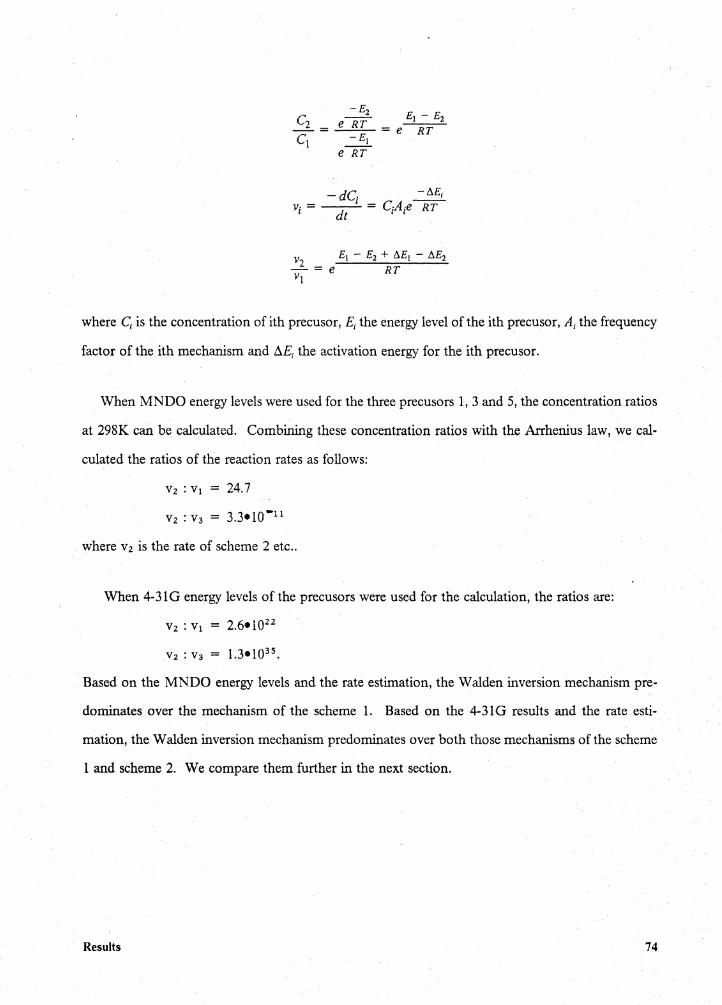
-dC1 -M; V· = --- = CA-e RT
l dt l l
where C1 is the concentration of ith precusor, E1 the energy level of the ith precusor, A1 the frequency
factor of the ith mechanism and 6.£1 the activation energy for the ith precusor.
When MNDO energy levels were used for the three precusors 1, 3 and 5, the concentration ratios
at 298K can be calculated. Combining these concentration ratios with the Arrhenius law, we cal-
culated the ratios of the reaction rates as follows:
V2: V1 = 24.7
. where v2 is the rate of scheme 2 etc ..
When 4-31 G energy levels of the precusors were used for the calculation, the ratios are:
Based on the MNDO energy levels and the rate estimation, the Walden inversion mechanism pre-
dominates over the mechanism of the scheme 1. Based on the 4-31G results and the rate esti-
mation, the Walden inversion mechanism predominates over both those mechanisms of the scheme
1 and scheme 2. We compare them further in the next section.
Results 74
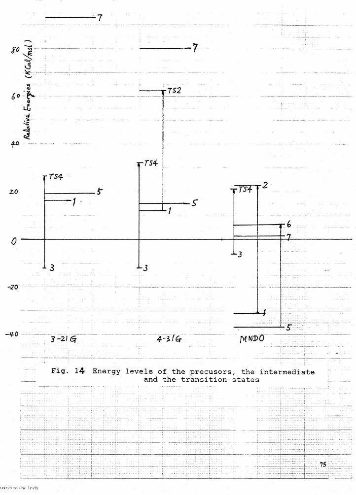
........._ ~
-----7
~ .. - -- -------
3 ~. __ :_ - -----·--···------------·----· .._, ~--··
·~ 60 ·t· -·11
cl ~··
TS4 · Z.()
0
3
-20
-l/-0 ---3-21 q
----7
----TS2
TS4-
--=r.=-s-.-+ --- 2
1-------s .___ ......... ,
3
J
---·-- ------------- ----- ---------------------+ ------s::::-'
f\1 NJ)Q-- -------·-- ... ---··-------
Fig. 14 Energy levels of the precusors, the intermediate and the transition states
;. \.
I - 1 ·•- • r i ~---------~-·---- ----·-- ---~ --- ---··-:--:-:~-~ -----:·::----·--- ---
. i-----~-----____;_----~----· __ ........:. ____ ·. _· ·~--_: ~-__:_--~-------
--· - - . - - - . -· l: . . - . -·. -~--·-----------"'----------- -----~-~--_..L ______ --------·--'·------------~----- .----·------- ----·-- ----·--------~-.J---~--·- -- -
t-~ --. r . i - .-t .. :::::::· :.t:·-
i·1uan·s ro till' Inch
-C---~---··
-- ·-' ~ •• -- - - . .L - 1
- _____ _J_ ____________ +---- ---·-------- -·-- --~ , - --i--,-- ....
--- ···t· t. - :·~:::.-:.!: ..
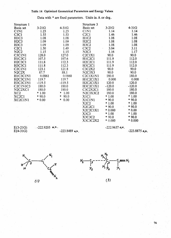
Table 14 Optimized Geometrical Parameters and Energy Values
Data with • are fixed parameters. Units in A or deg ..
Structure 1 Structure 3 Basis set 3-21G 4-31G Basis set 3-21G 4-3IG ClNl 1.25 1.25 ClNl 1.14 l.14 C3Cl 1.55 1.53 C2Cl 1.46 1.46 HIC3 l.08 1.08 HIC2 1.08 1.08 H2C3 1.09 1.09 H2C2 l.08 1.08 H3C3 l.09 1.09 H3C2 l.08 1.08 C2Cl l.50 1.49 C3C2 3.04 3.11 N2C2 1.15 l.15 N2C3 1.16 1.17 C3C1Nl 128.0 127.0 C2C1Xl 90.0 90.0 HlC3Cl 107.5 107.6 HlC2Cl 111.9 112.0 H2C3Cl 111.8 112.3 H2C2Cl 111.9 112.0 H3C3Cl 111.8 112.3 H3C2Cl 111.9 112.0 C2ClN1 123.1 121.8 C3C2X2 90.0 90.0 N2C2X 87.7 88. l N2C3X3 90.0 90.0 HIC3C1Nl 0.0861 0.0860 C2ClX1Nl 180.0 180.0 H2C3C1Nl 119.7 119.7 HlC2ClXl 0.000 0.000 H3C3C1Nl -119.5 -119.5 H2C2C1Xl 120.0 120.0 C2ClN1C3 180.0 180.0 H3C2C1Xl -120.0 -120.0 N2C2XC1 180.0 180.0 C3C2X2Cl 180.0 180.0 XC2 + 1.00 + l.00 N2C3X3C2 180.0 180.0 XC2Cl + 90.0 + 90.0 XlCl + 1.00 + 1.00 XC2C1Nl + 0.00 + 0.00 XlClNl + 90.0 + 90.0
X2C2 • 1.00 + l.00 X2C2Cl + 90.0 • 90.0 X2C2C1Xl • 0.000 • 0.00 X3C3 • 1.00 • 1.00 X3C3C2 + 90.0 + 90.0 X3C3C2X2 + 0.000 + 0.000
E(3-21G) -222.9205 ~.U·. -222.9657 tt..14. E(4-31G) -223.8489 4..U.. -223.8875 d..it.
(I) ( 3)
76

Table 14 Optimized Geometrical Parameters and Energy Values (continued)
Data with + are fixed parameters. Units in A or deg ..
Ref. Structilre Basis set ClNl C2Cl HC N2C3 HC2Cl XI Cl XlClNl C2C1Xl C2ClX1Nl HlC2ClXl H2C2 H2C2Cl H2C2C1Xl H3C2 H3C2Cl H3C2C1Xl X2C2 X2C2Cl X2C2C1Xl C3C2 C3C2X2 C3C2X2Cl X3C3 X3C3C2 X3C3C2X2 N2C3X3 N2C3X3C2
E(3-21G)
3-21G 1.14 1.46 1.08 1.17
110.3 + 1.00 + 90.0 + 90.0 + 180.0 +. 0.000
HC HC2Cl 120.0 BC HC2Cl
*-120.0 + 1.00 + 90.0 + 0.00 ... 8.00 + 90.0 + 180.0 + 1.00 + 90.0 + 0.00 + 90.0 + 180.0
-222 .. 9462 d..."'.
4-31G
H
N-C-----~-C-NI l 'J /\J. . I
H H
Monomer Basis set ClN C1C2 C2Hl ClC2Hl XCl XCIN C2ClX C2C1XN HlC2ClX H2C2C1X H3C2C1X H2C2 H3C2 H2C2Cl H3C2Cl
3-21G 1.14 1.46 1.08
110.2 + 1.00 + 90.0 + 90.0 + 180.0 + 0.000 + 120.0 •-120.0 C2Hl C2Hl C1C2Hl C1C2Hl
-131.1918 c:L.'-'.
4-31G
77
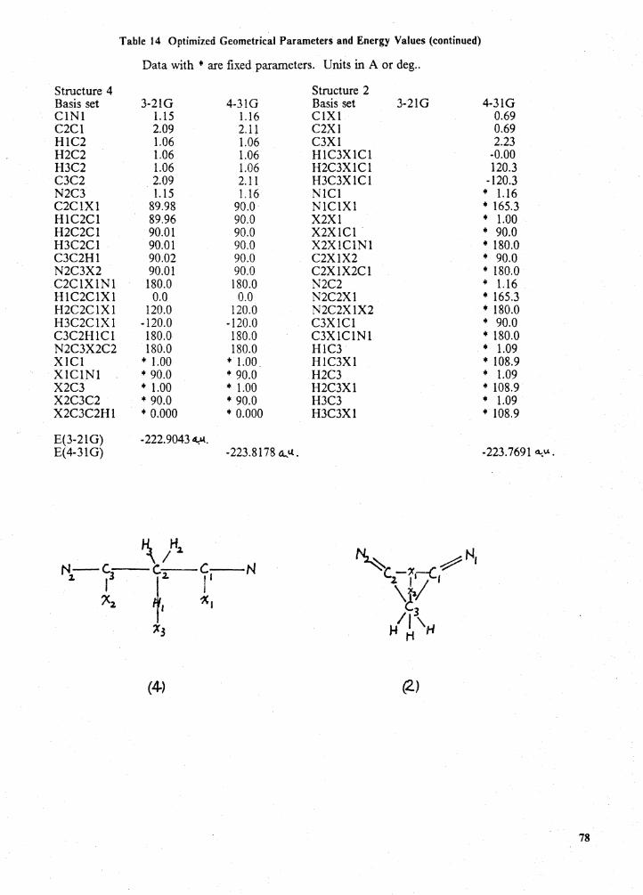
Structure 4 Basis set ClNl C2Cl H1C2 H2C2 H3C2 C3C2 N2C3 C2C1Xl HlC2Cl H2C2Cl H3C2Cl C3C2Hl N2C3X2 C2ClX1Nl HlC2ClXl H2C2C1Xl H3C2CIX1 C3C2HICI N2C3X2C2 XlCl XlClNl X2C3 X2C3C2 X2C3C2Hl
E(3-21G) E(4-31G)
Table 14 Optimized Geometrical Parameters and Energy Values (continued)
Data with + are fixed parameters. Units in A or deg ..
3-2lG 4-31G l.15 1.16 2.09 2.11 l.06 1.06 1.06 l.06 1.06 1.06 2.09 2.11 1.15 1.16
89.98 90.0 89.96 90.0 90.01 90.0 90.01 90.0 90.02 90.0 90.01 90.0 180.0 180.0
0.0 0.0 120.0 120.0
-120.0 -120.0 180.0 180.0 180.0 180.0
+ 1.00 + 1.00. + 90.0 + 90.0 + 1.00 + 1.00 + 90.0 + 90.0 + 0.000 + 0.000
-222.9043 ~.
(4)
-223.8178 4.,.U..
C--N I' -x,
Structure 2 Basis set 3-21G ClXl C2Xl C3Xl HlC3XlC1 H2C3XlC1 H3C3X1Cl NI Cl NlClXl X2Xl X2X1Cl X2XlC1Nl C2XIX2 C2XlX2Cl N2C2 N2C2Xl N2C2X1X2 C3X1Cl C3XlC1Nl H1C3 HlC3Xl H2C3 H2C3Xl H3C3 H3C3Xl
(2)
4-31G 0.69 0.69 2.23
-0.00 120.3
-120.3 + l.16 • 165.3 • 1.00 + 90.0 + 180.0 + 90.0 + 180.0 + 1.16 + 165.3 + 180.0 + 90.0 + 180.0 + 1.09 + 108.9 + 1.09 + 108.9 + 1.09 + 108.9
-223.769111:."'.
78
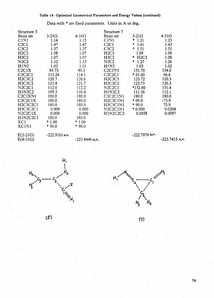
Table 14 Optimized Geometrical Parameters and Energy Values (continued)
Data with "' are fixed parameters. Units in A or deg ..
Structure 5 Structure 7 Basis set 3-21G 4-31G Basis set 3-21G 4-3IG CINl 1.14 l.15 CINI + 1.21 1.23 C2Cl 1.47 1.47 C2Cl + 1.41 l.43 C3C2 l.37 1.37 C3C2 + I.SI l.5I H2C3 1.08 1.07 H2C3 1.09 1.08 H3C3 1.07 1.07 H3C3 • H2C3 1.08 N2C2 1.32 1.33 N2C2 • 1.27 1.26 HIN2 1.02 1.0 l HIN2 1.03 1.02 C2CIX 89.75 90.3 C2CIN1 151.70 154.0 C3C2CI 113.24 114.1 C3C2CI + 61.60 66.6 H2C3C2 120.7 120.6 H2C3CI 123.72 I20.3 H3C3C2 121.4 121. 7 H3C3Cl 123.73 120.3 N2C2Cl 112.0 112.2 N2C2Cl •152.60 151.4 HIN2C2 109.3 110.4 HlN2C2 11 l.36 112.1 C2ClXNl 180.0 . 180.0 C3C2C1Nl 180.0 180.0 C3C2ClX 180.0 180.0 H2C3C1Nl •-90.0 -75.9 H2C3C2Cl 180.0 180.0 H3C3CIN1 + 90.0 75.9 H3C3C2Cl 0.000 0.000 N2C2C1Nl + 0.000 0.0204 N2C2ClX 0.000 0.000 HIN2C2C3 0.0058 0.0097 H1N2C2Cl 180.0 180.0 XCl • 1.00 + 1.00 XCINl + 90.0 + 90.0
E(3-21G) -222.9161 a.:-1t. -222.7979 o.i.t. E(4-31G) -223.8446 a...". -223.7415 4,,lt.
(S") (7)
79
Table 15 Comparison of the energy levels using the various computational methods, kcal/mol
Activation Energies
Scheme 1 (1-2) Scheme 3 (5-6) Scheme 2 (3-4)
3-21G
> 74.2 38.5
stabilizing Energies
3-21G Cyanoacetaldimine anion (1) 16.l Transition State (2) Cyanide anion-acetoni tri le complex (3) -12.2 Transition State {4) 26.3 Cyanoacetaldimine anion (5) 18.9 Transition State (6) Cyclopropanedi-imine anion (7) 93.1
Energies in column 3-21G Energies in column 4-31G Energy reference in MNDO
i
4t31G 5~.1
> 51
1f.J:. 7 43.8
I I
I
!
J-31G I I
~2.0
~2.1 I
-~2.2 ~1. 6
I I
:14. 7
MNDO 53.5 43.0 26.8
MNDO
-30.9
22.6
- 6.1
20.7
-36.6
6.4 I 19.4 1.6
relative t~ Ref. structure in Table 14. relative tJ TS (3) in colomn 3-21G. colomn see I Ref. 7. ·
80
Discussion
Based on our 4-31G results, the activation energy of the SN 2 mechanism (scheme 2) is 43.8
kcal/mol. This is lower than the 54.7 kcal/mol energy difference between precusor (5) and inter-
mediate (7) of scheme 3. The activation energy of scheme 3 must be larger than 54. 7 kcal/mol as
shown in Fig. 14.
•" ·'"
The energy level of precusor (3) in the SN2 mechanism, -12.2 kcal/mol (3-21G) is more stable
than those of (1), + 12.0 kcal/mol and (5), + 14.7 kcal/mol (3-21G) respectively. Similar results
are seen from the 4-31G results. Therefore, we conclude that the Walden inversion is the more
likely mechanism based on both its activation energy and the stability energy levels of the precusors
of scheme 1 and scheme 3 when either 3-21G or 4-31G energy levels are used. Comparison of the
energy levels using the various computational methods is shown in Table 15.
Even though not all parameters of the transition structure 2 (scheme 1) were optimized in our
4-31 G calculation, an approximate activation energy of scheme 1, 50.1 kcal/mol, was calculated and
this suggests that the Walden inversion (scheme 2) predominants over the mechanism suggested
by Jay et al.. Kinetic calculations using Andrades' MNDO results also show that the Walden in-
version is more likely than the mechanism of scheme 1.
Discussion 81
Contrary results were obtained for the relationship between the Walden inversion and the
mechanism of scheme 3 from MNDO and 4-31G results as shown by kinetic estimation as well as
by the stability energies of the precusors. However, the activation energies of the Walden inversion
is the lowest in both cases. In fact, if the activation energy of the process from (1) to (5) is included,
it shows that the mechanism of scheme 3 is even more unfavorable.
Based on this simplified kinetic estimation and our 4-31G results, we support the Walden in-
version as the most likely mechanism among the three suggested. It should be noted, however, that
solvent effects are not included in any of the theoretical calculations. Inclusion of salvation effects
could alter the reaction mechanism which would be predicted.
Discussion 82
Appendix A. Cartesian coordinates of the methanol
crystal
Appendix A. Cartesian coordinates of the methanol crystal 83
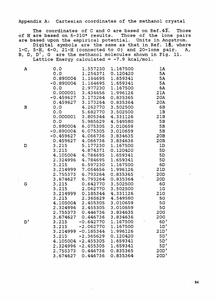
Appendix A: Cartesian coordinates of the methanol crystal
The coordinates of C and O are based on Ref. 45'. Those of H are based on 6-3 lG* results. Those of the lone pairs are based upon the empirical potential. Units in Angstrom.
Digital symbols are the same as that in Ref. 18, where 1-C, 5-H, 6-0, 21-H (connected to 0) and 20-lone pair. A, B, D, D', G are the methanol molecules shown in E'ig. 11.
A
B
D
G
D'
Lattice Energy calculated= -7.9 kcal/mol.
0.0 1.557230 0.0 1.254371 0.890004 1.164695
-0.890004 1.164695 0.0 2.977230 0.000001 3.434656
-0.459627 3.173264 0.459627 3.173264 0.0 4.262770 0.0 5.682770 0.000001 3.805344 0.0 5.985629 0.890004 6.075305
-0.890004 6.075305 -0.459627 4.066736 0.459627 4.066736 3.215 5.177230 3.215 -4.874371 4.105004 4.784695 2.324996 4.784695 3.215 6.597230 3.214999 7.054656 2.755373 6.793264 3.674627 6.793264 3.215 0.642770 3.215 2.062770 3.214999 0.185344 3.215 2.365629 4.105004 2.455305 2.324996 2.45530S 2.7SS373 0.446736 3.674627 0.446736 3.21S -0.642770 3.215 -2.062770 3.214999 -0~185344 3.21S -2.36S629 4.10S004 -2.45S305 2.324996 -2.455305 2.755373 0.446736 3.674627 0.446736
1.167500 0.120420 1.659341 1.659341 1.167500 1. 996126 0.835365 0.835364 3.S02SOO 3.S02SOO 4.331126 4.S49580 3.010659 3.010659 3.83463S 3.834636 1.167SOO 0.120420 1. 6S9341 l.6S9341 1.167SOO 1.996126 0.83S36S 0.835364 3.S02500 3.S02SOO 4.331126 4.549S80 3.0106S9 3.0106S9 3.83463S 3.834636 1.167SOO 1.167500 1. 996126 0.120420 1.659341 1.6S9341 0.83S36S 0.83S364
lA SA SA SA 6A
21A 20A 20A
6B lB
21B -SB SB SB
20B 20B
lD SD SD SD 6D
21D 20D 20D
6G lG
21G SG SG SG
20G 20G
6D' lD'
21D' SD' SD' SD'
20D' 20D'
84
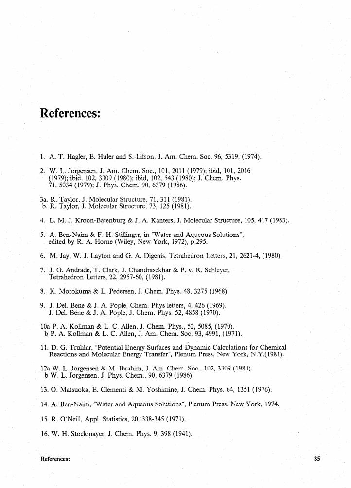
References:
1. A. T. Hagler, E. Huler and S. Lifson, J. Am. Chem. Soc. 96, 5319, (1974).
2. W. L. Jorgensen, J. Am. Chem. Soc., 101, 2011 (1979); ibid, 101, 2016 (1979); ibid, 102, 3309 (1980); ibid, 102, 543 (1980); J. Chem. Phys. 71, 5034 (1979); J. Phys. Chem. 90, 6379 (1986).
3a. R. Taylor, J. Molecular Structure, 71, 311 (1981). b. R. Taylor, J. Molecular Structure, 73, 125 (1981).
4. L. M. J. Kroon-Batenburg & J. A. Kanters, J. Molecular Structure, 105, 417 (1983).
5. A. Ben-Nairn. & F. H. Stillinger, in 'Water and Aqueous Solutions", edited by R. A. Home (Wiley, New York, 1972), p.295.
6. M. Jay, W. J. Layton and G. A. Digenis, Tetrahedron Letters, 21, 2621-4, (1980).
7. J. G. Andrade, T. Clark, J. Chandrasekhar & P. v. R. Schleyer, Tetrahedron Letters, 22, 2957-60, (1981).
8. K. Morokuma & L. Pedersen, J. Chem. Phys. 48, 3275 (1968).
9. J. Del. Bene & J. A. Pople, Chem. Phys letters, 4, 426 (1969). J. Del. Bene & J. A. Pople, J. Chem. Phys. 52, 4858 (1970).
lOa P.A. Kollman & L. C. Allen, J. Chem. Phys., 52, 5085, (1970). b P.A. Kollman & L. C. Allen, J. Am. Chem. Soc. 93, 4991, (1971).
11. D. G. Truhlar, "Potential Energy Surfaces and Dynamic Calculations for Chemical Reactions and Molecular Energy Transfer", Plenum Press, New York, N.Y.(1981).
12a W. L. Jorgensen & M. Ibrahim, J. Am. Chem. Soc., 102, 3309 (1980). b W. L. Jorgensen, J. Phys. Chem., 90, 6379 (1986).
13. 0. Matsuoka, E. Clementi & M.Yoshimine, J. Chem. Phys. 64, 1351 (1976).
14. A. Ben-Nairn., 'Water and Aqueous Solutions", Plenum Press, New York, 1974.
15. R. O'Neill, Appl. Statistics, 20, 338-345 (1971).
16. W. H. Stockrnayer, J. Chem. Phys. 9, 398 (1941).
References: 85
17a J. S. Rowlinson, Trans. Faraday Soc., 45, 974(1949). b J. S. Rowlinson, Trans. Faraday Soc., 47, 120 (1951). c J. S. Rowlinson, J. Chem. Phys., 19, 827 (1951).
18a Quantum Chemistry Program Exchange, No. 318, Chemisry Department, Indiana University, Bloomington, IN.
b Quantum Chemistry Program Exchange, No. 395, Chemisry Department, Indiana University, Bloomington, IN. ·
19. H. Popki.e, H. Kistenmacher & E. Clementi, J. Chem. Phys. 59, 1325 (1973).
20. J. D. Bernal & F. D. Fowler, J. Chem. Phys. 1, 515 (1933).
21. N. Bjerrum, Kgl. Danske Videnskab. Selskab, Mat.-Fys. Medd., 27, 1 (1951).
22. D. Eisenberg & W. Kauzmann, "The Structure and Properties of Water" (Oxford, U. P., New York. 1969), p. 139, 71.
23. T. Oie, G. M. Maggiora & R. E. Christoffersen, International J. of Quantum Chemistry: Quantum Biofogy Symposium 8, 1 (1981).
24. M. D~ Newton, J. Phys. Chem. 87, 4288 (1983).
25. B. R. Lentz & H. A. Scheraga, J. Chem. Phys. 58, 5296 (1973); 61, 3493, (1974).
26. K. T. No & M. S. John, J. Phys. Chem. 87, 226 (1983).
27. D. Hankins, J. W. Moskowitz & F. H. Stillinger, J. Chem. Phys. 53, 4544 (1970).
28. T. R. Dyke, K. M. Mack & J. S. Muenter, J. Chem. Phys., 66, 498 (1977).
29. L.A. Curtiss, D. J. Frurip & M. Blander, J. Chem. Phys. 71, 2703 (1979).
30. H. A. Gebbie, W. J. Burroughs, J. Chamberlain, J.E. Harries & R. G. Jones, Nature 221, 143 (1969).
31. G. S. Kell, G. E. McLaurin, & E. Whalley, J. Chem. Phys. 48, 3805 (1968); ibid. 49, 2839 (1968); G. S. Kell & G. E. McLaurin, ibid. 51, 4345 (1969).
32. J. H. Dymond & E. B. Smith, The Virial Coefficients of Gases (Clarendon, Oxford, 1969); F. G. Keyes, J. Chem. Phys. 15, 602 (1947).
33. J. D. Lambert & E. D. T. Strong, Proc. R. Soc. London Ser. A. 200, 566 (1950).
34. J.E. Lowder, J. Quant. Spectrosc. Radiat. Transfer, 10, 1085 (1970).
35. G. G. Gimmestad & G. W. F. Partlow, J. Quant. Spectrosc. Radiat. transfer, 12, 559 (1972).
36. K. D. Cook & J. W. Taylor, Int. J. Mass Spectrosc. Ion Phys., 30, 345 (1979).
37. J. D. Dill, L. C. Allen, W. C. Topp & l. A. Pople, J. Am. Chem. Soc., 97, 7220 (1975).
38. G. Brink& L Glasser, J. Compt. Chem. 2, 177.181 (1981).
39. M. D. Newton, G. A. Jeffrey & S. Takagi, J. Am. Chem. Soc. 101, 1997 (1979).
References: 86
40. L. Pauling, "The Nature of the Chemical Bondn, Cornell University Press, Ithaca, New York, 1960, p467.
41. S. W. Peterson & H. A. Levy, Acta Cryst., 10, 70 (1957).
42. E. Whalley, "The Hydrogen Bond" Vol.III, pp 1425-70, Edited by P. Schuster, G. Zundel & C. Sandorfy, North-Holland Publishing Company, 1976.
43. D. P. Santry, J. Am. Chem. Soc. 94, 8311 (1972).
44. R. M. Badger & S. H. Bauer; J. Chem Phys. 5, 839 (1937).
45. K. J. Tauer & W. N. Lipscomb, Acta Cryst., 5, 606 (1952).
46a W. L. Bragg, Proc. Roy. Soc. Al05, 370-386 (1924). b W. L. Bragg, ibid, Al06, 346-368 (1924).
47. W. H. Zachariasen, J. Chem. Phys. 1, 640-642 (1933).
48a S. Bhagavantam, Proc. Roy. Soc. Al24, 545-554 (1929). b S. Bhagavantam, ibid, A126, 143-154 (1930).
49. M. M. Julian and F. D. Bloss, Acta Cryst. A38, 167-169 (1982).
50. C. W. Bunn, Chemical Crystallography. Oxford University Press, London (1961).
51. D. E. Sands, Vectors and Tensors in Crystallography. Addison-Wesley Publishing Co.,Massachusetts. p126 (1982).
52. J. F. Nye, Physical Properties of Crystals. Oxford University Press, London (1957).
53. J. Yoshimura, Y. Ohgo & T. Sato, Bull. Chem. Soc. Japan, 38, 1809 (1965).
54. nThe Chemistry of the Cyano Group", Z. Rapoport, Ed., Chapter 6, Interscience Publishers, N. Y. ( 1970).
55a J. March, "Advanced Organic Chemistry: Reactions, Mechanisms and Structures", McGraw-Hill, N.Y. (1968) pp. 803 and 714.
b J. March, "Advanced Organic Chemistry: Reactions, Mechanisms and Structures", 2nd Ed., p.533, 962 McGraw Hill, N.Y. (1977).
56. R. B. Woodward & Hoffmann, Angew. Chem. Int. Ed. Engl., 10, 781 (1969).
57; P. D. Adeney, W. J. Bouma, L. Radom & W.R. Rodwell, J. Am. Chem. Soc., 102, 4069 (1980); W. J. Bouma, D. Poppinger & L. Radom, J. Am. Chem. Soc., 99, 6443 (1977); W. J. Bouma, M.A. Vincent & L. Radom, Int. J. Quantum Chem., 14, 767 (1978).
58. J. W. Viers, J.C. Schug & M. D. Stovall, J.Comput. Chem. 5, 598 (1984). 59. S. Wolfe, D. J. Mitchell & H.B. Schlegel, J. Am. Chem. Soc., 103, 7692 (1981); 103, 7694 (1981).
References: 87

The vita has been removed from the scanned document


![Table 1: TOYOLAC · 2020-02-03 · TPM / PCS-001 [Rev 20 / 2020-01-22] No. CAS No./ Chemical Formula Substance B63 90640-80-5 Anthracene oil B64 90640-81-6 Anthracene oil, anthracene](https://img.pdfslide.us/doc/110x75/5f64b2057ccdfd17d60cc655/table-1-toyolac-2020-02-03-tpm-pcs-001-rev-20-2020-01-22-no-cas-no-chemical.jpg)


![7,12 Dimethylbenz[a]Anthracene](https://img.pdfslide.us/doc/110x75/55cf857d550346484b8e9668/712-dimethylbenzaanthracene.jpg)