Embed Size (px)
Citation preview

Presentation Outline
Introduction to T-tests
Types of t-tests
Assumptions
Independent samples t-test
SPSS procedure
Interpretation of SPSS output
Presenting results from HMR
Paired samples t-test
SPSS procedure
Interpretation of SPSS output
Presenting results from HMR
Introduction
T-tests compare the values on some continuous
variable for two groups or on two occasions
Two types:
independent samples t-test – compares the
mean scores of two different groups of people or
conditions
paired samples t-test – compares the mean
scores for the same group of people on two
different occasions

Assumptions
Independence of observations – observations must not
be influenced by any other observation (e.g. behaviour of each member of the group influences all other group members)
Normal distribution
Random Sample (difficult in real-life research)
Homogeneity of Variance – variability of scores for each of
the groups is similar.
Levene’s test for equality of variances.
You want non significant result (Sig. greater than .05)

Research Question:
Is there a significant difference in the mean
criminal behaviour scores for violent and
non-violent offenders?
Independent Samples T-test

From the menu click on
Analyze
then select Compare
means
then Independent
Samples T test
Independent Samples T-test (SPSS)
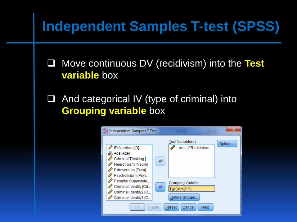
Move continuous DV (recidivism) into the Test
variable box
And categorical IV (type of criminal) into
Grouping variable box
Independent Samples T-test (SPSS)
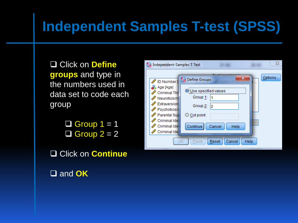
Independent Samples T-test (SPSS)
Click on Define
groups and type in
the numbers used in
data set to code each
group
Group 1 = 1
Group 2 = 2
Click on Continue
and OK
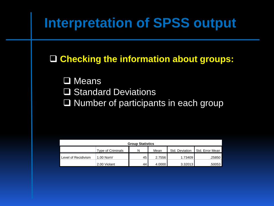
Interpretation of SPSS output
Group Statistics
Type of Criminals N Mean Std. Deviation Std. Error Mean
Level of Recidivism 1.00 NonV 45 2.7556 1.73409 .25850
2.00 Violant 44 4.0000 3.32013 .50053
Checking the information about groups:
Means
Standard Deviations
Number of participants in each group

Interpretation of SPSS output
Independent Samples Test
Levene's Test for Equality of
Variances t-test for Equality of Means
F Sig. t df Sig. (2-tailed)
Mean
Difference
Std. Error
Difference
95% Confidence Interval of the
Difference
Lower Upper
Level of Recidivism Equal variances assumed 5.335 .023 -2.223 87 .029 -1.24444 .55969 -2.35690 -.13199
Equal variances not
assumed
-2.209 64.513 .031 -1.24444 .56334 -2.36967 -.11921
Checking assumptions
Levene’s test for equality of variance (whether the variation
of scores for two groups is the same)
If Sig. value for Levene’s test > .05 – use the first line in the
table (Equal variance assumed)
If Sig. value for Levene’s test < or = .05 – use the second line
in the table (Equal variance not assumed)

Interpretation of SPSS output
Independent Samples Test
Levene's Test for Equality of
Variances t-test for Equality of Means
F Sig. t df Sig. (2-tailed)
Mean
Difference
Std. Error
Difference
95% Confidence Interval of the
Difference
Lower Upper
Level of Recidivism Equal variances assumed 5.335 .023 -2.223 87 .029 -1.24444 .55969 -2.35690 -.13199
Equal variances not
assumed
-2.209 64.513 .031 -1.24444 .56334 -2.36967 -.11921
Differences between groups
Check column Sig. (2-tailed)
If Sig. value > .05 – no significant difference between groups
If Sig. value < or = .05 – significant difference between groups

Calculating the effect size
The formula is: t2
Eta squared = -------------------------
t2 + (N1 + N2 -2)
-2.212
Eta squared = ---------------------------- = .05
-2.212 + (45 + 44 -2)
According to Cohen (1988)
.01 = small effect
.06 = medium effect
.14 = large effect

Presenting results
An independent samples t-test was conducted to
compare the criminal behaviour (recidivism) scores
doe violent and non violent offenders. There was a
significant difference in score between the two
groups of offenders, t(87) = -2.21, p < .05, two-tailed
with violent offenders (M = 4.00, SD = 3.32) scoring
higher than non violent offenders (M = 2.76, SD =
3.32). The magnitude of the differences in the means
(mean difference = -1.24, 95% CI: -2.37 to -.12) was
small (eta squared = .05)

Paired samples t-test
A Paired samples t-test – one group of participants
measured on two different occasions or under two
different conditions (e.g., pre-test & post-test; Time 1 &
Time 2)
Research question – Is there a significant change in
prisoners’ criminal social identity scores after 2 year
sentence in high security prison? Does the process of
prisonization have an impact on prisoners’ criminal identity
test scores?
You need:
1 categorical IV (Time 1, Time 2)
1 continuous DV (criminal social identity test scores)

Paired samples t-test (SPSS)
From the menu
click on Analyze
then select
Compare Means
then Paired
Samples T test

Density
Paired samples t-test (SPSS)
Click on the 2 variables that you are interested in
comparing for each subject (criminal identity,
criminal identity 2) and move them into Paired
Variables box
Click OK

Interpretation of SPSS output
Descriptive Statistics
Correlations
Paired Samples Statistics
Mean N Std. Deviation Std. Error Mean
Pair 1 Criminal Identity 18.7303 89 8.93762 .94739
Criminal Identity2 26.3146 89 9.84031 1.04307
Paired Samples Correlations
N Correlation Sig.
Pair 1 Criminal Identity & Criminal
Identity2
89 .941 .000

Interpretation of SPSS output
Paired Samples Test
Paired Differences
t df Sig. (2-tailed) Mean Std. Deviation Std. Error Mean
95% Confidence Interval of the
Difference
Lower Upper
Pair 1 Criminal Identity - Criminal
Identity2
-7.58427 3.35006 .35511 -8.28997 -6.87857 -21.358 88 .000
Differences between Time 1 & Time 2
Check column Sig. (2-tailed)
If Sig. value > .05 – no significant difference
If Sig. value < or = .05 – significant difference

Calculating the effect size
The formula is: t2
Eta squared = -------------------------
t2 + (N - 1)
-21.362
Eta squared = ---------------------------- = .84
-21.362 + (88 - 1)
According to Cohen (1988)
.01 = small effect
.06 = medium effect
.14 = large effect

Presenting results
A paired samples t-test was conducted to
evaluate the impact of the prisonization process
on prisoners’ scores on the criminal social
identity. There was a significant increase in
criminal social identity scores from Time 1 (M =
18.73, SD = 8.94) to Time 2 (M = 26.31, SD =
9.84), t(88) = -21.36, p < .001 (two-tailed). The
mean increase in criminal social identity scores
was -7.58 with a 95% confidence interval
ranging from -8.29 to -6.88. The eta squared
statistic (.84) indicated a large effect size.