Embed Size (px)
Citation preview
232
Learning Objectives:
• Understand the similar logic underlying various test statistics• Determine the degrees of freedom• Calculate a two-sample t test for independent samples and equal sample sizes• Use a table to interpret the calculated t• Report results in APA format
A Two-Sample Study
Now that you know how to calculate the standard error of the difference between the means, you are ready to calculate a two-sample t test. This time, however, we will calculate σM1 − M2
from raw data. Recall that calculating a σM1 − M2
first involves calculating the σM for each population. And calculating a σM for a population first involves calculating the σest for each population based on sample data. Therefore, this module will include a lot of calculations.
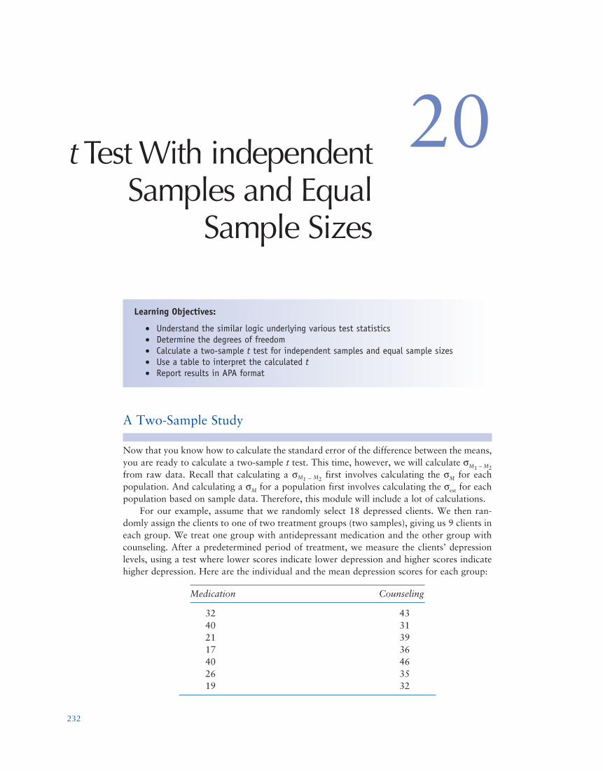
For our example, assume that we randomly select 18 depressed clients. We then ran-domly assign the clients to one of two treatment groups (two samples), giving us 9 clients in each group. We treat one group with antidepressant medication and the other group with counseling. After a predetermined period of treatment, we measure the clients’ depression levels, using a test where lower scores indicate lower depression and higher scores indicate higher depression. Here are the individual and the mean depression scores for each group:
Medication Counseling
32 43 40 31 21 39 17 36 40 46 26 35 19 32
t Test With independent Samples and Equal
Sample Sizes
20
ModulE 20: t TEST WiTh indEpEndEnT SaMplES and Equal SaMplE SizES 233
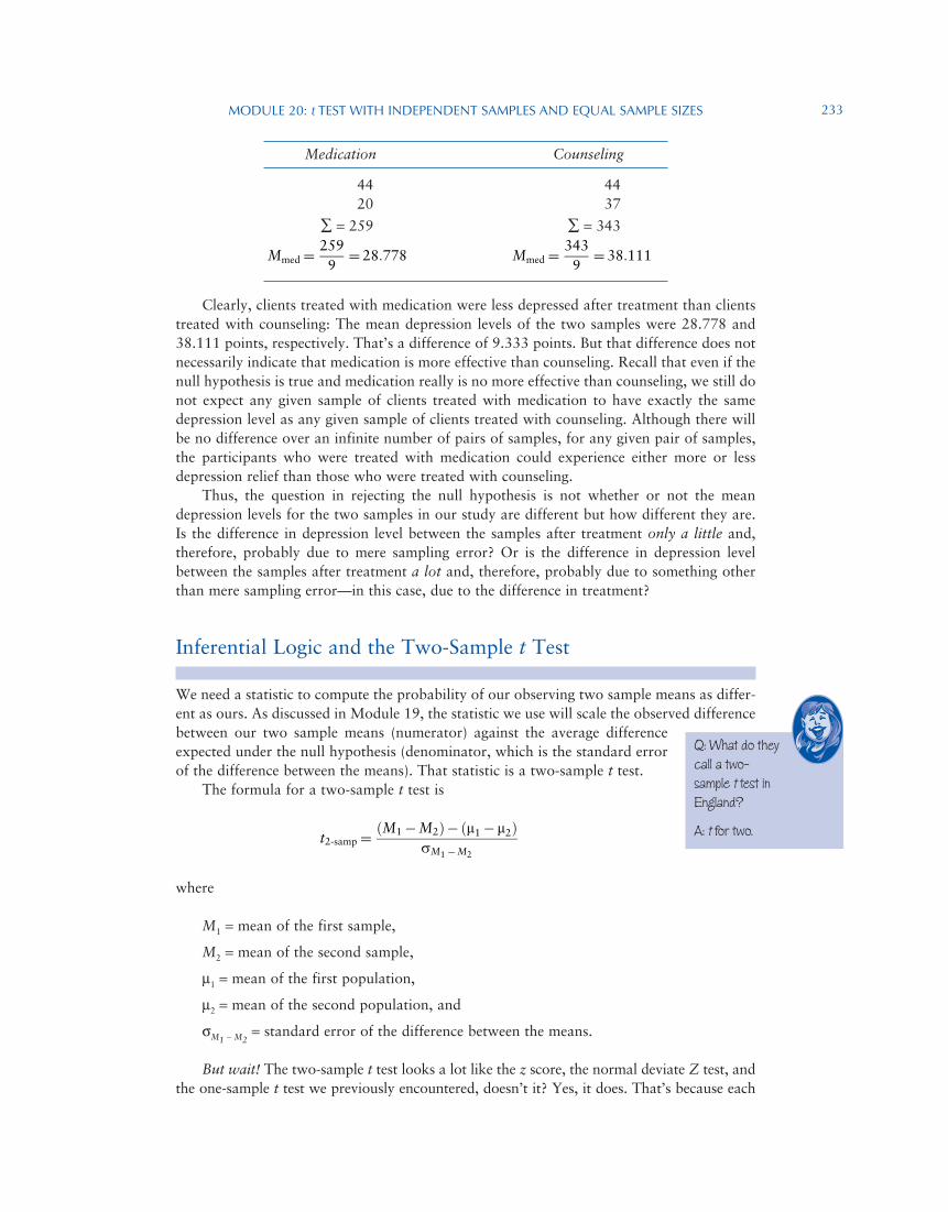
Medication Counseling
44 44 20 37
∑ = 259 ∑ = 343
Mmed =2599
= 28:778 Mmed =3439
= 38:111
Clearly, clients treated with medication were less depressed after treatment than clients treated with counseling: The mean depression levels of the two samples were 28.778 and 38.111 points, respectively. That’s a difference of 9.333 points. But that difference does not necessarily indicate that medication is more effective than counseling. Recall that even if the null hypothesis is true and medication really is no more effective than counseling, we still do not expect any given sample of clients treated with medication to have exactly the same depression level as any given sample of clients treated with counseling. Although there will be no difference over an infinite number of pairs of samples, for any given pair of samples, the participants who were treated with medication could experience either more or less depression relief than those who were treated with counseling.
Thus, the question in rejecting the null hypothesis is not whether or not the mean depression levels for the two samples in our study are different but how different they are. Is the difference in depression level between the samples after treatment only a little and, therefore, probably due to mere sampling error? Or is the difference in depression level between the samples after treatment a lot and, therefore, probably due to something other than mere sampling error—in this case, due to the difference in treatment?
Inferential Logic and the Two-Sample t Test
We need a statistic to compute the probability of our observing two sample means as differ-ent as ours. As discussed in Module 19, the statistic we use will scale the observed difference between our two sample means (numerator) against the average difference expected under the null hypothesis (denominator, which is the standard error of the difference between the means). That statistic is a two-sample t test.
The formula for a two-sample t test is
t2-samp =ðM1 −M2Þ− ðm1 − m2Þ
sM1 −M2
where
M1 = mean of the first sample,
M2 = mean of the second sample,
µ1 = mean of the first population,
µ2 = mean of the second population, and
σM1 − M2 = standard error of the difference between the means.
But wait! The two-sample t test looks a lot like the z score, the normal deviate Z test, and the one-sample t test we previously encountered, doesn’t it? Yes, it does. That’s because each
Q: What do they call a two-sample t test in England?
A: t for two.
ModulE 20: t TEST WiTh indEpEndEnT SaMplES and Equal SaMplE SizES234
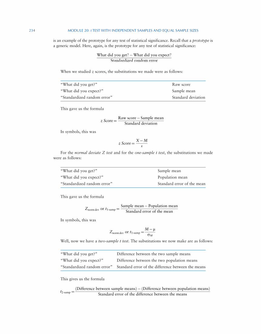
is an example of the prototype for any test of statistical significance. Recall that a prototype is a generic model. Here, again, is the prototype for any test of statistical significance:
What did you get?−What did you expect?Standardized random error
When we studied z scores, the substitutions we made were as follows:
“What did you get?” Raw score
“What did you expect?” Sample mean
“Standardized random error” Standard deviation
This gave us the formula
z Score= Raw score− Sample mean
Standard deviation
In symbols, this was
z Score= X−M
s
For the normal deviate Z test and for the one-sample t test, the substitutions we made were as follows:
“What did you get?” Sample mean
“What did you expect?” Population mean
“Standardized random error” Standard error of the mean
This gave us the formula
Znormdev or t1-samp =Sample mean− Population mean
Standard error of the mean
In symbols, this was
Znormdev or t1-samp =M− msM
Well, now we have a two-sample t test. The substitutions we now make are as follows:
“What did you get?” Difference between the two sample means
“What did you expect?” Difference between the two population means
“Standardized random error” Standard error of the difference between the means
This gives us the formula
t2-samp =ðDifference between sample meansÞ− ðDifference between population meansÞ
Standard error of the difference between the means
ModulE 20: t TEST WiTh indEpEndEnT SaMplES and Equal SaMplE SizES 235
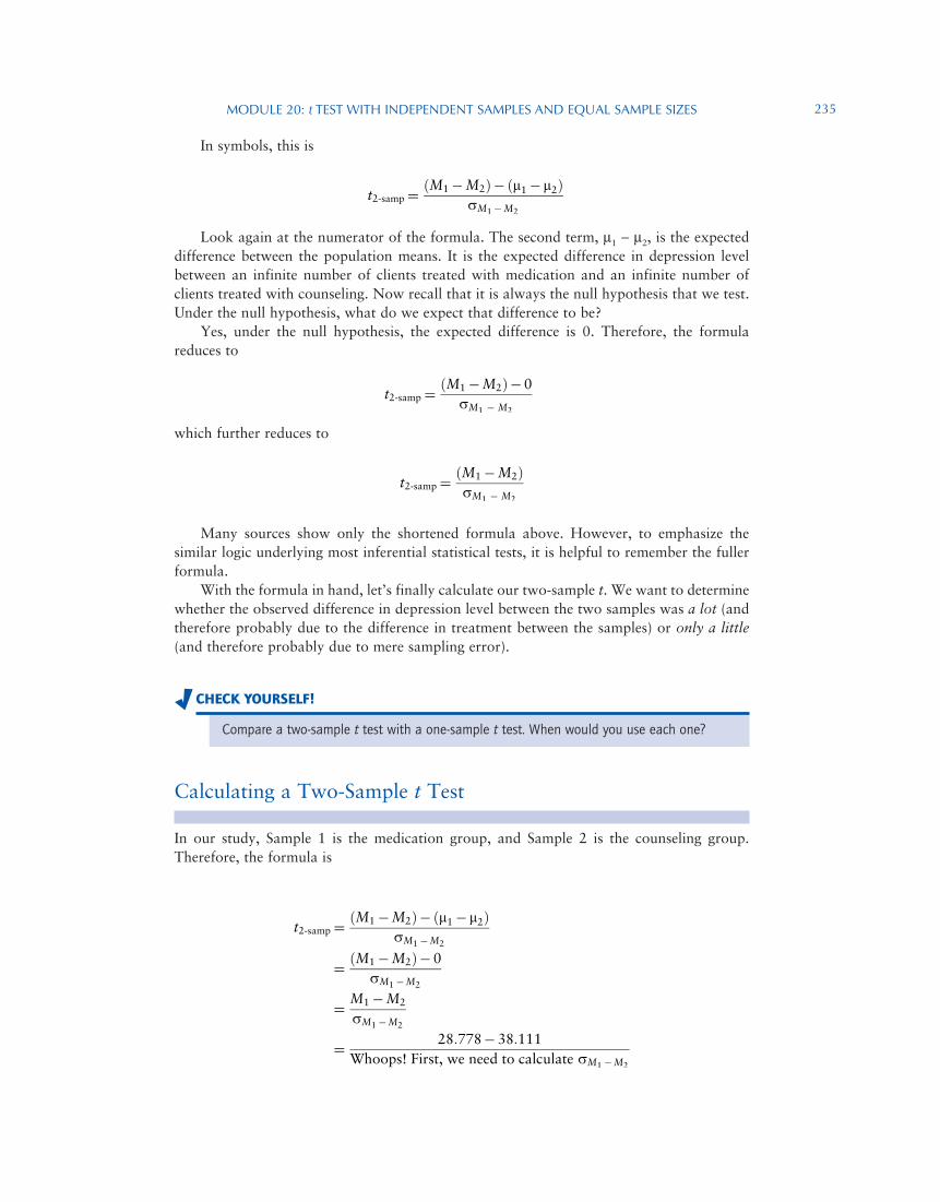
In symbols, this is
t2-samp =ðM1 −M2Þ− ðm1 − m2Þ
sM1 −M2
Look again at the numerator of the formula. The second term, µ1 − µ2, is the expected difference between the population means. It is the expected difference in depression level between an infinite number of clients treated with medication and an infinite number of clients treated with counseling. Now recall that it is always the null hypothesis that we test. Under the null hypothesis, what do we expect that difference to be?
Yes, under the null hypothesis, the expected difference is 0. Therefore, the formula reduces to
t2-samp =ðM1 −M2Þ− 0
sM1 − M2
which further reduces to
t2-samp =ðM1 −M2ÞsM1 − M2
Many sources show only the shortened formula above. However, to emphasize the similar logic underlying most inferential statistical tests, it is helpful to remember the fuller formula.
With the formula in hand, let’s finally calculate our two-sample t. We want to determine whether the observed difference in depression level between the two samples was a lot (and therefore probably due to the difference in treatment between the samples) or only a little (and therefore probably due to mere sampling error).
CheCk Yourself!
Compare a two-sample t test with a one-sample t test. When would you use each one?
Calculating a Two-Sample t Test
In our study, Sample 1 is the medication group, and Sample 2 is the counseling group. Therefore, the formula is
t2-samp =ðM1 −M2Þ− ðm1 − m2Þ
sM1 −M2
= ðM1 −M2Þ− 0sM1 −M2
= M1 −M2
sM1 −M2
= 28:778− 38:111Whoops! First, we need to calculate sM1 −M2
ModulE 20: t TEST WiTh indEpEndEnT SaMplES and Equal SaMplE SizES236
In this module, we are restricting ourselves to studies in which sample sizes are equal and the samples are independent. Recall that when samples are independent and sample sizes are equal, the formula for σM1 − M2
is
sM1 −M2 =ffiffiffiffiffiffiffiffiffiffiffiffiffiffiffiffiffiffiffiffiffiffiffis2
M1+s2
M2
q
where
σM1 = the standard error of the mean of the first population and
σM2 = the standard error of the mean of the second population.
But what is the σM for each population? Yes, unfortunately, we first have to compute each of those as well. Recall that the formula for σM is
sffiffiffin
p orsestffiffiffi
np
where σest = σ estimated from s.Because we do not know the population standard deviation (σ) for either
population, we have to use the second formula, which uses the estimated population standard deviation (σest) for each population.
But what is the estimated population standard deviation for each popula-tion? Yes, we estimate it from the sample data. That’s where we must begin our calculations, so let’s do that now.
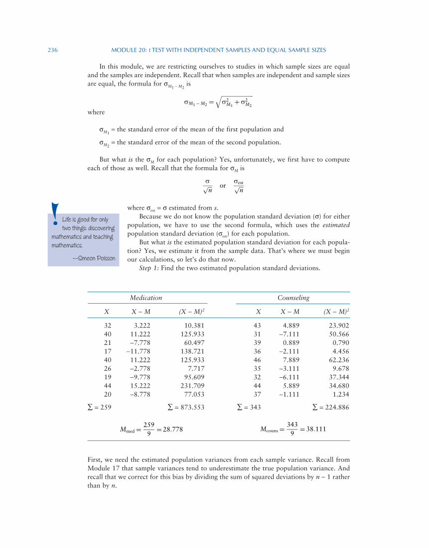
Step 1: Find the two estimated population standard deviations.
Medication Counseling
X X − M (X − M)2 X X − M (X − M)2
32 3.222 10.381 43 4.889 23.90240 11.222 125.933 31 −7.111 50.56621 −7.778 60.497 39 0.889 0.79017 −11.778 138.721 36 −2.111 4.45640 11.222 125.933 46 7.889 62.23626 −2.778 7.717 35 −3.111 9.67819 −9.778 95.609 32 −6.111 37.34444 15.222 231.709 44 5.889 34.68020 −8.778 77.053 37 −1.111 1.234
∑ = 259 ∑ = 873.553 ∑ = 343 ∑ = 224.886
Mmed =
2599
= 28:778
Mcouns =3439
= 38:111
First, we need the estimated population variances from each sample variance. Recall from Module 17 that sample variances tend to underestimate the true population variance. And recall that we correct for this bias by dividing the sum of squared deviations by n − 1 rather than by n.
Life is good for only two things: discovering
mathematics and teaching mathematics.
—Simeon Poisson
ModulE 20: t TEST WiTh indEpEndEnT SaMplES and Equal SaMplE SizES 237
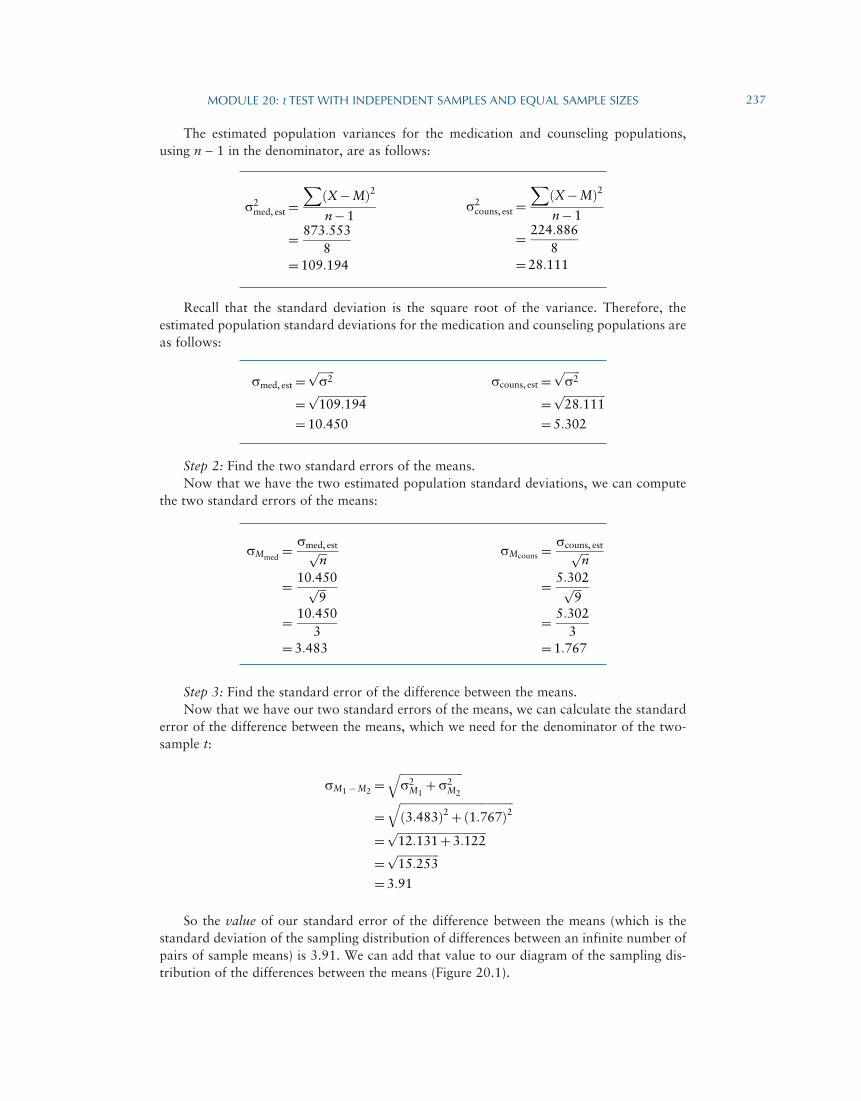
The estimated population variances for the medication and counseling populations, using n − 1 in the denominator, are as follows:
s2med, est =
XðX−MÞ2
n−1
= 873:5538
= 109:194
s2couns, est =
XðX−MÞ2
n− 1
= 224:8868
= 28:111
Recall that the standard deviation is the square root of the variance. Therefore, the estimated population standard deviations for the medication and counseling populations are as follows:
smed, est =ffiffiffiffiffiffis2
p
=ffiffiffiffiffiffiffiffiffiffiffiffiffiffiffiffiffiffi109:194
p
= 10:450
scouns, est =ffiffiffiffiffiffis2
p
=ffiffiffiffiffiffiffiffiffiffiffiffiffiffiffi28:111
p
= 5:302
Step 2: Find the two standard errors of the means.Now that we have the two estimated population standard deviations, we can compute
the two standard errors of the means:
sMmed=
smed, estffiffiffin
p
= 10:450ffiffiffi9
p
= 10:4503
= 3:483
sMcouns =scouns, estffiffiffi
np
= 5:302ffiffiffi9
p
= 5:3023
= 1:767
Step 3: Find the standard error of the difference between the means.Now that we have our two standard errors of the means, we can calculate the standard
error of the difference between the means, which we need for the denominator of the two-sample t:
sM1 −M2 =ffiffiffiffiffiffiffiffiffiffiffiffiffiffiffiffiffiffiffiffiffiffiffis2
M1+s2
M2
q
=ffiffiffiffiffiffiffiffiffiffiffiffiffiffiffiffiffiffiffiffiffiffiffiffiffiffiffiffiffiffiffiffiffiffiffiffiffiffiffiffiffið3:483Þ2 + ð1:767Þ2
q
=ffiffiffiffiffiffiffiffiffiffiffiffiffiffiffiffiffiffiffiffiffiffiffiffiffiffiffiffiffiffiffiffi12:131+3:122
p
=ffiffiffiffiffiffiffiffiffiffiffiffiffiffiffi15:253
p
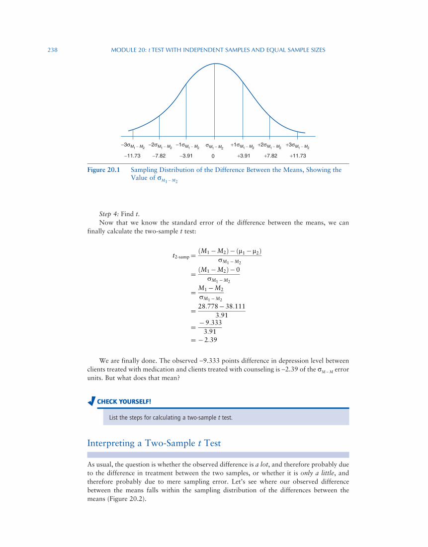
= 3:91
So the value of our standard error of the difference between the means (which is the standard deviation of the sampling distribution of differences between an infinite number of pairs of sample means) is 3.91. We can add that value to our diagram of the sampling dis-tribution of the differences between the means (Figure 20.1).
ModulE 20: t TEST WiTh indEpEndEnT SaMplES and Equal SaMplE SizES238
Step 4: Find t.Now that we know the standard error of the difference between the means, we can
finally calculate the two-sample t test:
t2-samp =ðM1 −M2Þ− ðm1 − m2Þ
sM1 −M2
= ðM1 −M2Þ− 0sM1 −M2
= M1 −M2
sM1 −M2
= 28:778− 38:1113:91
= −9:3333:91
= − 2:39
We are finally done. The observed −9.333 points difference in depression level between clients treated with medication and clients treated with counseling is −2.39 of the σM − M error units. But what does that mean?
CheCk Yourself!
List the steps for calculating a two-sample t test.
Interpreting a Two-Sample t Test
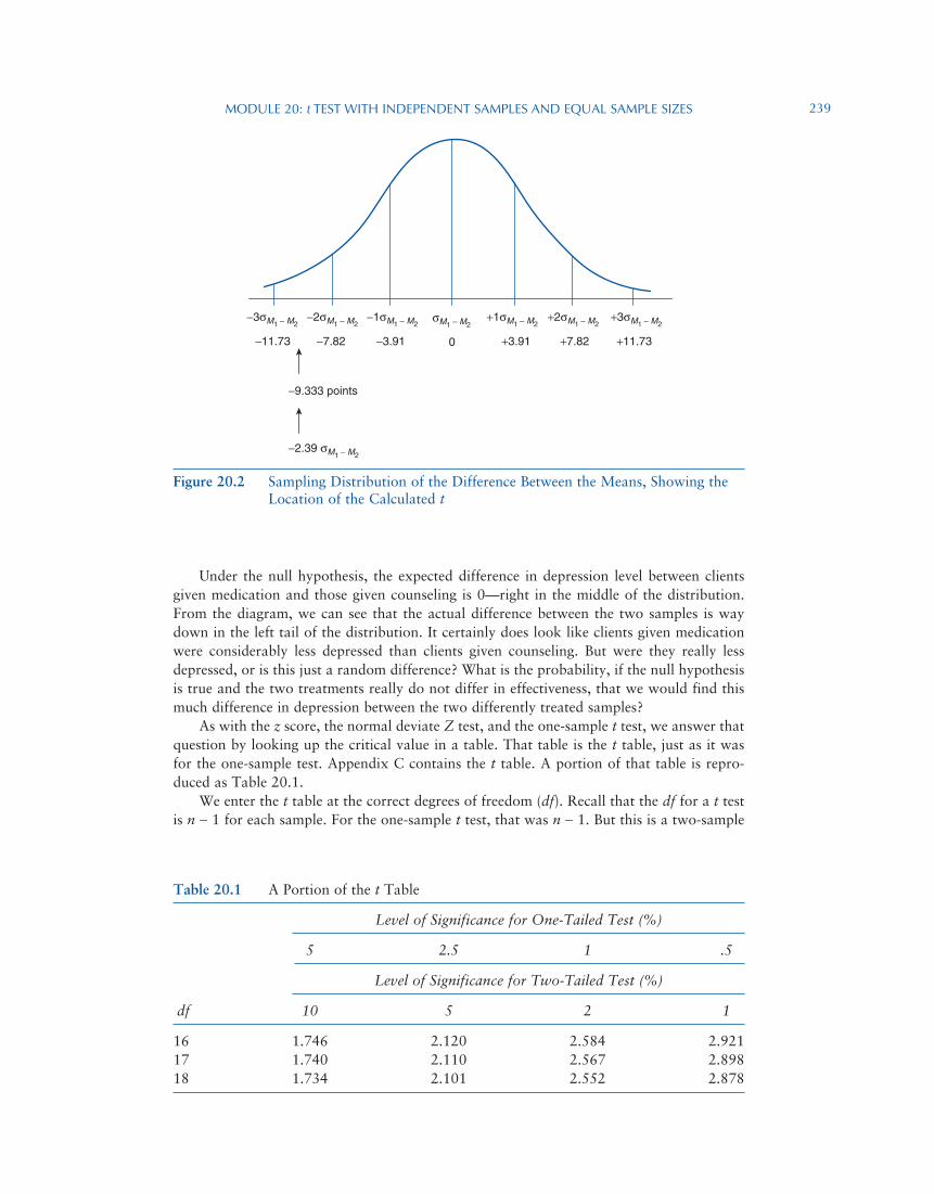
As usual, the question is whether the observed difference is a lot, and therefore probably due to the difference in treatment between the two samples, or whether it is only a little, and therefore probably due to mere sampling error. Let’s see where our observed difference between the means falls within the sampling distribution of the differences between the means (Figure 20.2).
−1σM1 − M2+1σM1 − M2
σM1 − M2+2σM1 − M2
+3σM1 − M2−2σM1 − M2
−3σM1 − M2
−3.91 +3.910 +7.82 +11.73−7.82−11.73
Figure 20.1 Sampling Distribution of the Difference Between the Means, Showing the Value of σM1 − M2
ModulE 20: t TEST WiTh indEpEndEnT SaMplES and Equal SaMplE SizES 239
Under the null hypothesis, the expected difference in depression level between clients given medication and those given counseling is 0—right in the middle of the distribution. From the diagram, we can see that the actual difference between the two samples is way down in the left tail of the distribution. It certainly does look like clients given medication were considerably less depressed than clients given counseling. But were they really less depressed, or is this just a random difference? What is the probability, if the null hypothesis is true and the two treatments really do not differ in effectiveness, that we would find this much difference in depression between the two differently treated samples?
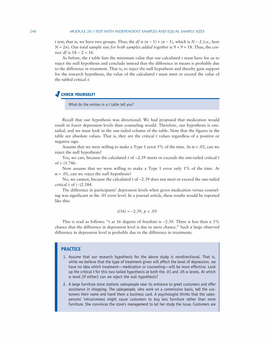
As with the z score, the normal deviate Z test, and the one-sample t test, we answer that question by looking up the critical value in a table. That table is the t table, just as it was for the one-sample test. Appendix C contains the t table. A portion of that table is repro-duced as Table 20.1.
We enter the t table at the correct degrees of freedom (df). Recall that the df for a t test is n − 1 for each sample. For the one-sample t test, that was n − 1. But this is a two-sample
−1σM1 − M2+1σM1 − M2
σM1 − M2+2σM1 − M2
+3σM1 − M2−2σM1 − M2
−2.39 σM1 − M2
−3σM1 − M2
−3.91 +3.910 +7.82 +11.73−7.82
−9.333 points
−11.73
Figure 20.2 Sampling Distribution of the Difference Between the Means, Showing the Location of the Calculated t
Table 20.1 A Portion of the t Table
Level of Significance for One-Tailed Test (%)
5 2.5 1 .5
Level of Significance for Two-Tailed Test (%)
df 10 5 2 1
16 1.746 2.120 2.584 2.92117 1.740 2.110 2.567 2.89818 1.734 2.101 2.552 2.878
ModulE 20: t TEST WiTh indEpEndEnT SaMplES and Equal SaMplE SizES240
t test; that is, we have two groups. Thus, the df is (n − 1) + (n − 1), which is N − 2 (i.e., here N = 2n). Our total sample size for both samples added together is 9 + 9 = 18. Thus, the cor-rect df is 18 − 2 = 16.
As before, the t table lists the minimum value that our calculated t must have for us to reject the null hypothesis and conclude instead that the difference in means is probably due to the difference in treatment. That is, to reject the null hypothesis and thereby gain support for the research hypothesis, the value of the calculated t must meet or exceed the value of the tabled critical t.
CheCk Yourself!
What do the entries in a t table tell you?
Recall that our hypothesis was directional: We had proposed that medication would result in lower depression levels than counseling would. Therefore, our hypothesis is one-tailed, and we must look in the one-tailed column of the table. Note that the figures in the table are absolute values. That is, they are the critical t values regardless of a positive or negative sign.
Assume that we were willing to make a Type 1 error 5% of the time. At α = .05, can we reject the null hypothesis?
Yes, we can, because the calculated t of −2.39 meets or exceeds the one-tailed critical t of (−)1.746.
Now assume that we were willing to make a Type 1 error only 1% of the time. At α = .01, can we reject the null hypothesis?
No, we cannot, because the calculated t of −2.39 does not meet or exceed the one-tailed critical t of (−)2.584.
The difference in participants’ depression levels when given medication versus counsel-ing was significant at the .05 error level. In a journal article, these results would be reported like this:
t(16) = −2.39, p < .05
This is read as follows: “t at 16 degrees of freedom is −2.39. There is less than a 5% chance that the difference in depression level is due to mere chance.” Such a large observed difference in depression level is probably due to the difference in treatments.
Practice 1. Assume that our research hypothesis for the above study is nondirectional. That is,
while we believe that the type of treatment given will affect the level of depression, we have no idea which treatment—medication or counseling—will be more effective. Look up the critical t for this two-tailed hypothesis at both the .01 and .05 α levels. At which α level (if either) can we reject the null hypothesis?
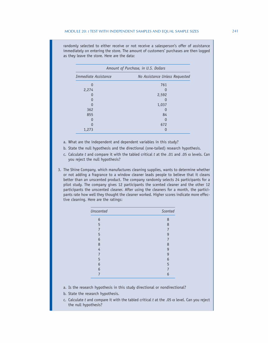
2. A large furniture store stations salespeople near its entrance to greet customers and offer assistance in shopping. The salespeople, who work on a commission basis, tell the cus-tomers their name and hand them a business card. A psychologist thinks that the sales-persons’ intrusiveness might cause customers to buy less furniture rather than more furniture. She convinces the store’s management to let her study the issue. Customers are
ModulE 20: t TEST WiTh indEpEndEnT SaMplES and Equal SaMplE SizES 241
randomly selected to either receive or not receive a salesperson’s offer of assistance immediately on entering the store. The amount of customers’ purchases are then logged as they leave the store. Here are the data:
Amount of Purchase, in U.S. Dollars
Immediate Assistance No Assistance Unless Requested
0 761 2,274 0 0 2,592 0 0 0 1,037 362 0 855 84 0 0 0 672 1,273 0
a. What are the independent and dependent variables in this study?
b. State the null hypothesis and the directional (one-tailed) research hypothesis.
c. Calculate t and compare it with the tabled critical t at the .01 and .05 α levels. Can you reject the null hypothesis?
3. The Shine Company, which manufactures cleaning supplies, wants to determine whether or not adding a fragrance to a window cleaner leads people to believe that it cleans better than an unscented product. The company randomly selects 24 participants for a pilot study. The company gives 12 participants the scented cleaner and the other 12 participants the unscented cleaner. After using the cleaners for a month, the partici-pants rate how well they thought the cleaner worked. Higher scores indicate more effec-tive cleaning. Here are the ratings:
Unscented Scented
6 85 87 75 96 78 84 97 95 66 56 77 6
a. Is the research hypothesis in this study directional or nondirectional?
b. State the research hypothesis.
c. Calculate t and compare it with the tabled critical t at the .05 α level. Can you reject the null hypothesis?
ModulE 20: t TEST WiTh indEpEndEnT SaMplES and Equal SaMplE SizES242
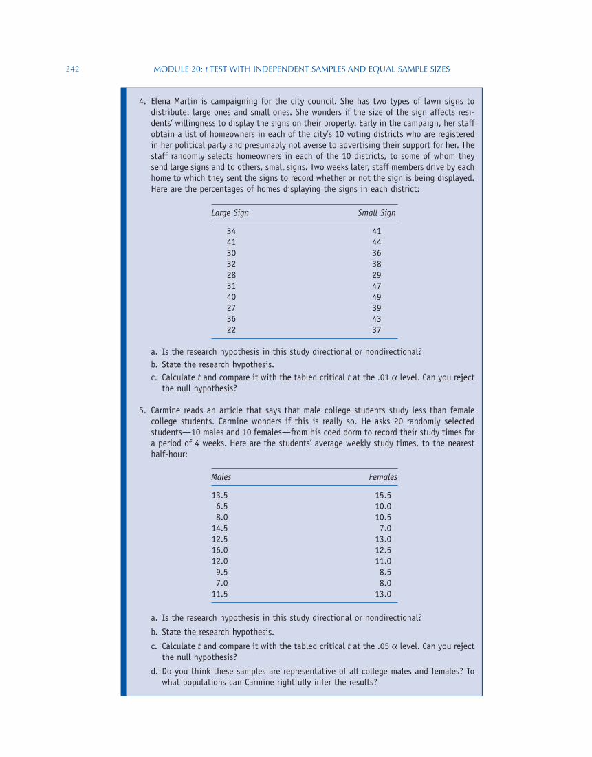
4. Elena Martin is campaigning for the city council. She has two types of lawn signs to distribute: large ones and small ones. She wonders if the size of the sign affects resi-dents’ willingness to display the signs on their property. Early in the campaign, her staff obtain a list of homeowners in each of the city’s 10 voting districts who are registered in her political party and presumably not averse to advertising their support for her. The staff randomly selects homeowners in each of the 10 districts, to some of whom they send large signs and to others, small signs. Two weeks later, staff members drive by each home to which they sent the signs to record whether or not the sign is being displayed. Here are the percentages of homes displaying the signs in each district:
Large Sign Small Sign
34 4141 4430 3632 3828 2931 4740 4927 3936 4322 37
a. Is the research hypothesis in this study directional or nondirectional?b. State the research hypothesis.c. Calculate t and compare it with the tabled critical t at the .01 α level. Can you reject
the null hypothesis?
5. Carmine reads an article that says that male college students study less than female college students. Carmine wonders if this is really so. He asks 20 randomly selected students—10 males and 10 females—from his coed dorm to record their study times for a period of 4 weeks. Here are the students’ average weekly study times, to the nearest half-hour:
Males Females
13.5 15.5 6.5 10.0 8.0 10.5 14.5 7.0 12.5 13.0 16.0 12.5 12.0 11.0 9.5 8.5 7.0 8.0 11.5 13.0
a. Is the research hypothesis in this study directional or nondirectional?
b. State the research hypothesis.
c. Calculate t and compare it with the tabled critical t at the .05 α level. Can you reject the null hypothesis?
d. Do you think these samples are representative of all college males and females? To what populations can Carmine rightfully infer the results?
ModulE 20: t TEST WiTh indEpEndEnT SaMplES and Equal SaMplE SizES 243
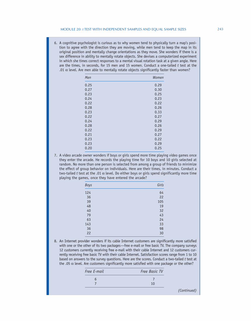
6. A cognitive psychologist is curious as to why women tend to physically turn a map’s posi-tion to agree with the direction they are moving, while men tend to keep the map in its original position and mentally change orientations as they move. She wonders if there is a sex difference in ability to mentally rotate objects. She devises a computerized experiment in which she times correct responses to a mental visual rotation task at a given angle. Here are the times, in seconds, for 15 men and 15 women. Conduct a one-tailed t test at the .01 α level. Are men able to mentally rotate objects significantly faster than women?
Men Women
0.25 0.290.27 0.300.23 0.250.24 0.230.22 0.220.28 0.260.23 0.330.22 0.270.24 0.290.28 0.260.22 0.290.21 0.270.23 0.220.23 0.290.20 0.25
7. A video arcade owner wonders if boys or girls spend more time playing video games once they enter the arcade. He records the playing time for 10 boys and 10 girls selected at random. No more than one person is selected from among a group of friends to minimize the effect of group behavior on individuals. Here are their times, in minutes. Conduct a two-tailed t test at the .01 α level. Do either boys or girls spend significantly more time playing the games, once they have entered the arcade?
Boys Girls
124 64 36 22 39 105 48 19 40 32 79 43 63 24143 33 36 98 22 30
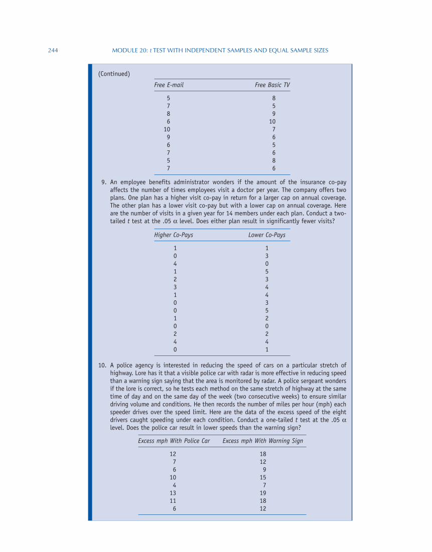
8. An Internet provider wonders if its cable Internet customers are significantly more satisfied with one or the other of its two packages—free e-mail or free basic TV. The company surveys 12 customers currently receiving free e-mail with their cable Internet and 12 customers cur-rently receiving free basic TV with their cable Internet. Satisfaction scores range from 1 to 10 based on answers to the survey questions. Here are the scores. Conduct a two-tailed t test at the .05 α level. Are customers significantly more satisfied with one package or the other?
Free E-mail Free Basic TV
6 77 10
(Continued)
244 ModulE 20: t TEST WiTh indEpEndEnT SaMplES and Equal SaMplE SizES
(Continued)
Free E-mail Free Basic TV
5 8 7 5 8 9 6 1010 7 9 6 6 5 7 6 5 8 7 6
9. An employee benefits administrator wonders if the amount of the insurance co-pay affects the number of times employees visit a doctor per year. The company offers two plans. One plan has a higher visit co-pay in return for a larger cap on annual coverage. The other plan has a lower visit co-pay but with a lower cap on annual coverage. Here are the number of visits in a given year for 14 members under each plan. Conduct a two-tailed t test at the .05 α level. Does either plan result in significantly fewer visits?
Higher Co-Pays Lower Co-Pays
1 10 34 01 52 33 41 40 30 51 20 02 24 40 1
10. A police agency is interested in reducing the speed of cars on a particular stretch of highway. Lore has it that a visible police car with radar is more effective in reducing speed than a warning sign saying that the area is monitored by radar. A police sergeant wonders if the lore is correct, so he tests each method on the same stretch of highway at the same time of day and on the same day of the week (two consecutive weeks) to ensure similar driving volume and conditions. He then records the number of miles per hour (mph) each speeder drives over the speed limit. Here are the data of the excess speed of the eight drivers caught speeding under each condition. Conduct a one-tailed t test at the .05 α level. Does the police car result in lower speeds than the warning sign?
Excess mph With Police Car Excess mph With Warning Sign
12 18 7 12 6 910 15 4 713 1911 18 6 12
ModulE 20: t TEST WiTh indEpEndEnT SaMplES and Equal SaMplE SizES 245
Looking Ahead
As we saw in Module 17, the ability to reject the null hypothesis depends not only on how different the observed group means are but also on what level of Type 1 error you are will-ing to accept. In Module 23, we will look at this concept of error in more detail, just as we did in Module 18. As it turns out, dichotomous decisions (reject/do not reject) are less mean-ingful than reports of actual Type 1 error.
SPSS Connection
Download the file data_depression relief due to med couns.sav from www.sagepub.com/steinberg2e. These data are used in the textbook example.
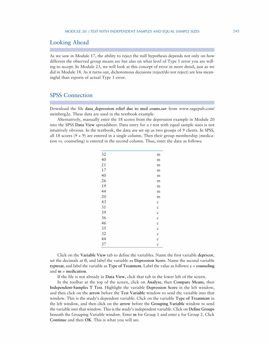
Alternatively, manually enter the 18 scores from the depression example in Module 20 into the SPSS Data View spreadsheet. Data entry for a t test with equal sample sizes is not intuitively obvious. In the textbook, the data are set up as two groups of 9 clients. In SPSS, all 18 scores (9 + 9) are entered in a single column. Then their group membership (medica-tion vs. counseling) is entered in the second column. Thus, enter the data as follows:
32 m40 m21 m17 m40 m26 m19 m44 m20 m43 c31 c39 c36 c46 c35 c32 c44 c37 c
Click on the Variable View tab to define the variables. Name the first variable deprscor, set the decimals at 0, and label the variable as Depression Score. Name the second variable typtreat, and label the variable as Type of Treatment. Label the value as follows: c = counseling and m = medication.
If the file is not already in Data View, click that tab in the lower left of the screen.In the toolbar at the top of the screen, click on Analyze, then Compare Means, then
Independent-Samples T Test. Highlight the variable Depression Score in the left window, and then click on the arrow before the Test Variable window to send the variable into that window. This is the study’s dependent variable. Click on the variable Type of Treatment in the left window, and then click on the arrow before the Grouping Variable window to send the variable into that window. This is the study’s independent variable. Click on Define Groups beneath the Grouping Variable window. Enter m for Group 1 and enter c for Group 2. Click Continue and then OK. This is what you will see.
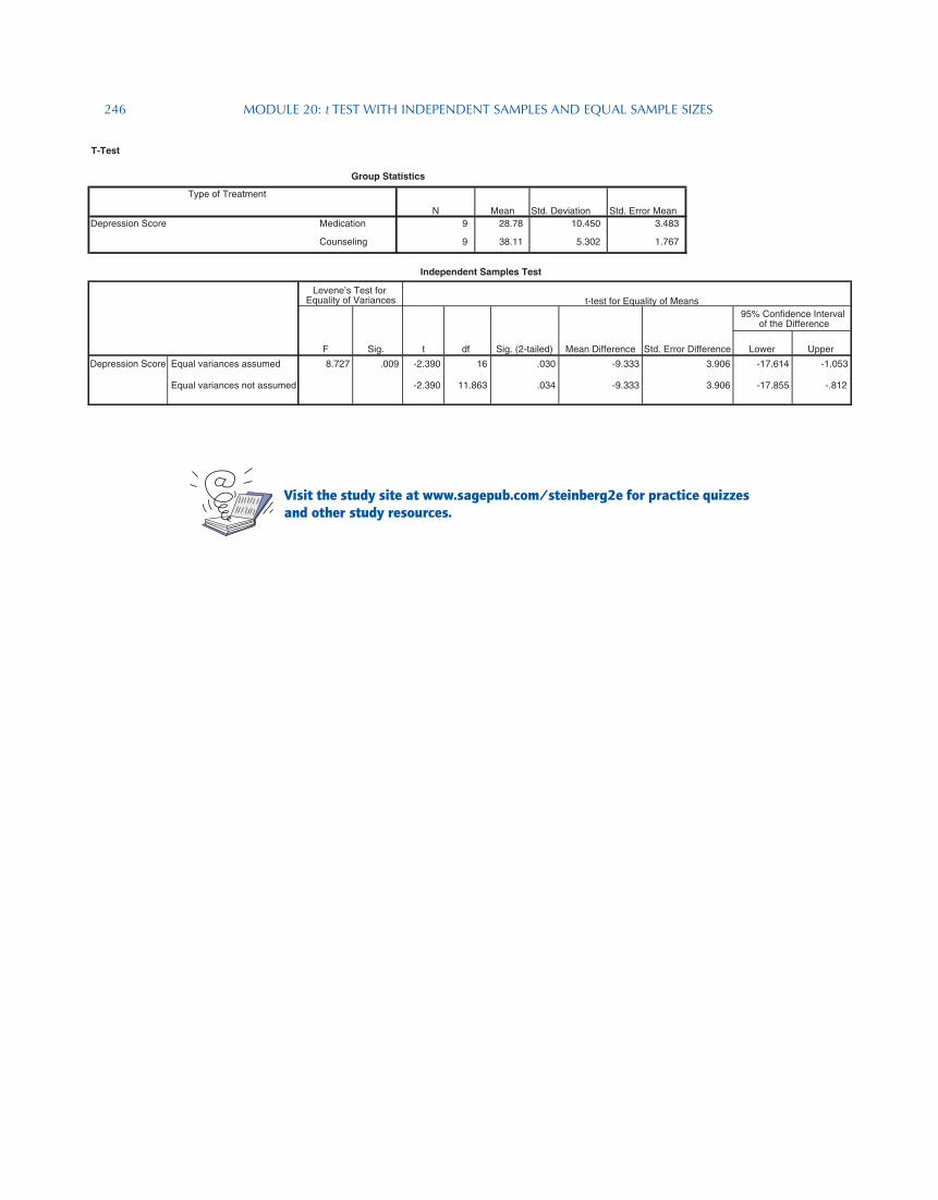
246 ModulE 20: t TEST WiTh indEpEndEnT SaMplES and Equal SaMplE SizES
T-Test
N Mean Std. Deviation Std. Error MeanMedication 9 28.78 10.450 3.483
Counseling 9 38.11 5.302 1.767
Lower Upper
Equal variances assumed 8.727 .009 -2.390 16 .030 -9.333 3.906 -17.614 -1.053
Equal variances not assumed -2.390 11.863 .034 -9.333 3.906 -17.855 -.812
Depression Score
t df Sig. (2-tailed) Mean Difference Std. Error Difference
95% Confidence Interval of the Difference
Group Statistics
Type of Treatment
Depression Score
Independent Samples Test
Levene’s Test for Equality of Variances t-test for Equality of Means
F Sig.
Visit the study site at www.sagepub.com/steinberg2e for practice quizzes and other study resources.