Published in The Astrophysical Journal Supplement: 227 (2016) 23Preprint typeset using LATEX style AASTeX6 v. 1.0

MAPS OF THE MAGELLANIC CLOUDS FROM COMBINED SOUTH POLE TELESCOPE AND PLANCKDATA

T. M. Crawford1,2, R. Chown3, G. P. Holder3, K. A. Aird4, B. A. Benson5,1,2, L. E. Bleem6,1,J. E. Carlstrom1,7,6,2,8, C. L. Chang6,1,2, H-M. Cho9, A. T. Crites1,2,11, T. de Haan3,10, M. A. Dobbs3,

E. M. George10,12, N. W. Halverson13, N. L. Harrington10, W. L. Holzapfel10, Z. Hou1,2, J. D. Hrubes4,R. Keisler1,7,15, L. Knox16, A. T. Lee10,14, E. M. Leitch1,2, D. Luong-Van4, D. P. Marrone17, J. J. McMahon18,

S. S. Meyer1,2,8,7, L. M. Mocanu1,2, J. J. Mohr19,20,12, T. Natoli1,7,21, S. Padin1,2, C. Pryke22, C. L. Reichardt10,23,J. E. Ruhl24, J. T. Sayre24,13, K. K. Schaffer1,8,25, E. Shirokoff10,1,2, Z. Staniszewski24,26, A. A. Stark27,

K. T. Story1,7,15,28, K. Vanderlinde3,21,29, J. D. Vieira30,31, and R. Williamson1,2

1Kavli Institute for Cosmological Physics, University of Chicago, Chicago, IL, USA 606372Department of Astronomy and Astrophysics, University of Chicago, Chicago, IL, USA 606373Department of Physics, McGill University, Montreal, Quebec H3A 2T8, Canada4University of Chicago, Chicago, IL, USA 606375Fermi National Accelerator Laboratory, MS209, P.O. Box 500, Batavia, IL 605106High Energy Physics Division, Argonne National Laboratory, Argonne, IL, USA 604397Department of Physics, University of Chicago, Chicago, IL, USA 606378Enrico Fermi Institute, University of Chicago, Chicago, IL, USA 606379SLAC National Accelerator Laboratory, 2575 Sand Hill Road, Menlo Park, CA 94025

10Department of Physics, University of California, Berkeley, CA, USA 9472011California Institute of Technology, Pasadena, CA, USA 9112512Max-Planck-Institut fur extraterrestrische Physik, 85748 Garching, Germany13Department of Astrophysical and Planetary Sciences and Department of Physics, University of Colorado, Boulder, CO, USA 8030914Physics Division, Lawrence Berkeley National Laboratory, Berkeley, CA, USA 9472015Kavli Institute for Particle Astrophysics and Cosmology, Stanford University, 452 Lomita Mall, Stanford, CA 9430516Department of Physics, University of California, Davis, CA, USA 9561617Steward Observatory, University of Arizona, 933 North Cherry Avenue, Tucson, AZ 8572118Department of Physics, University of Michigan, Ann Arbor, MI, USA 4810919Faculty of Physics, Ludwig-Maximilians-Universitat, 81679 Munchen, Germany20Excellence Cluster Universe, 85748 Garching, Germany21Dunlap Institute for Astronomy & Astrophysics, University of Toronto, 50 St George St, Toronto, ON, M5S 3H4, Canada22Department of Physics, University of Minnesota, Minneapolis, MN, USA 5545523School of Physics, University of Melbourne, Parkville, VIC 3010, Australia24Physics Department, Center for Education and Research in Cosmology and Astrophysics, Case Western Reserve University,Cleveland, OH,

USA 4410625Liberal Arts Department, School of the Art Institute of Chicago, Chicago, IL, USA 6060326Jet Propulsion Laboratory, California Institute of Technology, Pasadena, CA 91109, USA27Harvard-Smithsonian Center for Astrophysics, Cambridge, MA, USA 0213828Dept. of Physics, Stanford University, 382 Via Pueblo Mall, Stanford, CA 9430529Department of Astronomy & Astrophysics, University of Toronto, 50 St George St, Toronto, ON, M5S 3H4, Canada30Astronomy Department, University of Illinois at Urbana-Champaign, 1002 W. Green Street, Urbana, IL 61801, USA31Department of Physics, University of Illinois Urbana-Champaign, 1110 W. Green Street, Urbana, IL 61801, USA

ABSTRACT

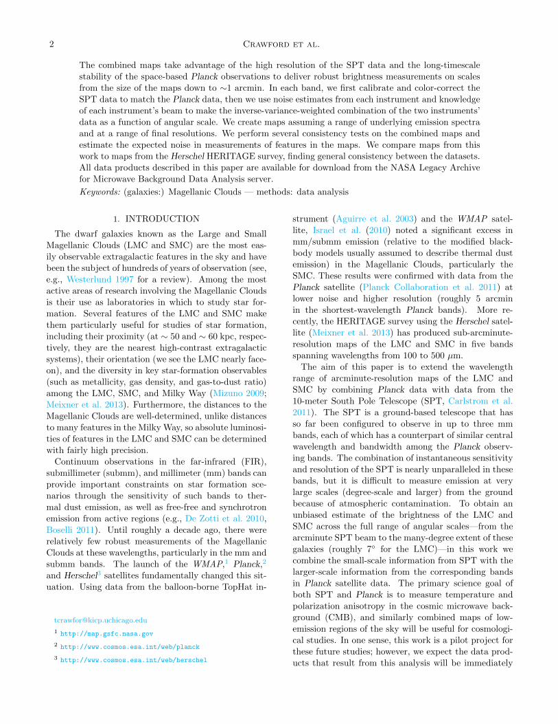
We present maps of the Large and Small Magellanic Clouds from combined South Pole Telescope

(SPT) and Planck data. The Planck satellite observes in nine bands, while the SPT data used in thiswork were taken with the three-band SPT-SZ camera, The SPT-SZ bands correspond closely to threeof the nine Planck bands, namely those centered at 1.4, 2.1, and 3.0 mm. The angular resolution ofthe Planck data ranges from 5 to 10 arcmin, while the SPT resolution ranges from 1.0 to 1.7 arcmin.

arX

iv:1

605.

0096

6v2

[as

tro-

ph.G

A]

9 D

ec 2

016

FERMILAB-PUB-16-158-AE-PPD (accepted)

2 Crawford et al.

The combined maps take advantage of the high resolution of the SPT data and the long-timescale

stability of the space-based Planck observations to deliver robust brightness measurements on scales

from the size of the maps down to ∼1 arcmin. In each band, we first calibrate and color-correct the

SPT data to match the Planck data, then we use noise estimates from each instrument and knowledge

of each instrument’s beam to make the inverse-variance-weighted combination of the two instruments’

data as a function of angular scale. We create maps assuming a range of underlying emission spectra

and at a range of final resolutions. We perform several consistency tests on the combined maps and

estimate the expected noise in measurements of features in the maps. We compare maps from this

work to maps from the Herschel HERITAGE survey, finding general consistency between the datasets.

All data products described in this paper are available for download from the NASA Legacy Archive

for Microwave Background Data Analysis server.

Keywords: (galaxies:) Magellanic Clouds — methods: data analysis

1. INTRODUCTION

The dwarf galaxies known as the Large and Small

Magellanic Clouds (LMC and SMC) are the most eas-

ily observable extragalactic features in the sky and have

been the subject of hundreds of years of observation (see,

e.g., Westerlund 1997 for a review). Among the most

active areas of research involving the Magellanic Clouds

is their use as laboratories in which to study star for-

mation. Several features of the LMC and SMC make

them particularly useful for studies of star formation,

including their proximity (at ∼ 50 and ∼ 60 kpc, respec-

tively, they are the nearest high-contrast extragalactic

systems), their orientation (we see the LMC nearly face-

on), and the diversity in key star-formation observables

(such as metallicity, gas density, and gas-to-dust ratio)

among the LMC, SMC, and Milky Way (Mizuno 2009;

Meixner et al. 2013). Furthermore, the distances to the

Magellanic Clouds are well-determined, unlike distances

to many features in the Milky Way, so absolute luminosi-

ties of features in the LMC and SMC can be determined

with fairly high precision.

Continuum observations in the far-infrared (FIR),

submillimeter (submm), and millimeter (mm) bands can

provide important constraints on star formation sce-

narios through the sensitivity of such bands to ther-

mal dust emission, as well as free-free and synchrotron

emission from active regions (e.g., De Zotti et al. 2010,

Boselli 2011). Until roughly a decade ago, there were

relatively few robust measurements of the Magellanic

Clouds at these wavelengths, particularly in the mm and

submm bands. The launch of the WMAP,1 Planck,2

and Herschel3 satellites fundamentally changed this sit-

uation. Using data from the balloon-borne TopHat in-

tcrawfor@kicp.uchicago.edu

1 http://map.gsfc.nasa.gov

2 http://www.cosmos.esa.int/web/planck

3 http://www.cosmos.esa.int/web/herschel

strument (Aguirre et al. 2003) and the WMAP satel-

lite, Israel et al. (2010) noted a significant excess in

mm/submm emission (relative to the modified black-

body models usually assumed to describe thermal dust

emission) in the Magellanic Clouds, particularly the

SMC. These results were confirmed with data from the

Planck satellite (Planck Collaboration et al. 2011) at

lower noise and higher resolution (roughly 5 arcmin

in the shortest-wavelength Planck bands). More re-

cently, the HERITAGE survey using the Herschel satel-

lite (Meixner et al. 2013) has produced sub-arcminute-

resolution maps of the LMC and SMC in five bands

spanning wavelengths from 100 to 500 µm.

The aim of this paper is to extend the wavelength

range of arcminute-resolution maps of the LMC and

SMC by combining Planck data with data from the

10-meter South Pole Telescope (SPT, Carlstrom et al.

2011). The SPT is a ground-based telescope that has

so far been configured to observe in up to three mm

bands, each of which has a counterpart of similar central

wavelength and bandwidth among the Planck observ-

ing bands. The combination of instantaneous sensitivity

and resolution of the SPT is nearly unparalleled in these

bands, but it is difficult to measure emission at very

large scales (degree-scale and larger) from the ground

because of atmospheric contamination. To obtain an

unbiased estimate of the brightness of the LMC and

SMC across the full range of angular scales—from the

arcminute SPT beam to the many-degree extent of these

galaxies (roughly 7 for the LMC)—in this work we

combine the small-scale information from SPT with the

larger-scale information from the corresponding bands

in Planck satellite data. The primary science goal of

both SPT and Planck is to measure temperature and

polarization anisotropy in the cosmic microwave back-

ground (CMB), and similarly combined maps of low-

emission regions of the sky will be useful for cosmologi-

cal studies. In one sense, this work is a pilot project for

these future studies; however, we expect the data prod-

ucts that result from this analysis will be immediately

SPT-Planck maps of the Magellanic Clouds 3

useful to a wide range of astronomical applications.

This paper is structured as follows. In Section 2,

we describe the SPT and Planck instruments and data

products. In Section 3, we describe the procedure we

use to combine the two data sets into a single map in

each observing band. In Section 4, we present the com-

bined maps and perform a number of quality-control

checks. In Section 5, we compare the combined maps

with FIR/submm maps from the Herschel HERITAGE

survey. We conclude in Section 6.

2. INSTRUMENTS, DATA, AND PROCESSING

2.1. SPT

The SPT is a 10-meter telescope located within

1 km of the geographical South Pole, at the National

Science Foundation Amundsen-Scott South Pole sta-

tion. The telescope is designed for millimeter and sub-

millimeter observations of faint, diffuse sources, in par-

ticular anisotropy in the CMB. From 2007 to 2011, the

instrument at the focus of the SPT was the SPT-SZ cam-

era, which consisted of 960 detectors in three wavelength

bands centered at roughly 1.4, 2.0, and 3.2 mm (center

frequencies of roughly 220, 150, and 95 GHz). The main

lobe of the instrument beam, or point-spread function,

is closely approximated by an azimuthally symmetric,

two-dimensional Gaussian. The main-lobe full width

at half maximum (FWHM) measured on bright point

sources in survey fields (which includes a contribution

from day-to-day pointing variations) is equal to 1.0, 1.2,

and 1.7 arcmin at 1.4, 2.0, and 3.2 mm, respectively.

2.1.1. SPT Observations of the Magellanic Clouds

In 2011 November, parts of three observing days were

spent on dedicated observations of fields centered on

the Magellanic Clouds. The bulk of the time—roughly

20 hours—was spent on the LMC, with approximately

three hours spent on the SMC. The LMC field was de-

fined as an 8-by-8 region centered at R.A. 80, dec-

lination −68.5. The SMC field was defined as a 5-

by-5 region centered at R.A. 15, declination −72.5.

As with most fields observed with the SPT, these obser-

vations were conducted by scanning the telescope back

and forth in azimuth then taking a small (6 arcmin)

step in elevation. Because of the geographical location

of the telescope, this corresponds to scanning in right as-

cension and stepping in declination. At the scan speed

used for these observations (∼ 0.4/s on the sky), this

scan pattern covers the LMC field in 90 minutes and the

SMC field in 45 minutes. We refer to each individual 90-

or 45-minute set of scans as an “observation.”

2.1.2. Data Processing

Detector data are processed into maps individually for

each observation and wavelength band. The processing

pipeline used in this work is described in detail in Schaf-

fer et al. (2011); we summarize it briefly here. For each

observation, data that pass cuts are flat-fielded (by ad-

justing the data from each detector according to the re-

sponse of that detector to an internal calibration source)

and filtered. Using inverse-variance weighting, the data

are binned into pixels based on the value of the tele-

scope boresight pointing in every data sample and the

known physical locations of the detectors in the focal

plane. The maps for this work are made in the oblique

Lambert equal-area azimuthal (ZEA) projection, with a

pixel scale of 0.25 arcmin.

The filtering applied to the data consists of three

steps, the first two of which are primarily to suppress the

effects of atmospheric noise. First, a fifth-order polyno-

mial is fit to the data from each detector in each scan

and then subtracted from that data. Next, at every

time sample, the mean across a detector module (there

are six modules in the SPT-SZ camera, each with 160

detectors of a given frequency) and two spatial gradi-

ents across that module are calculated and subtracted

from the data of each detector on that module. Finally,

a Fourier-domain low-pass filter is applied to each de-

tector’s data to avoid aliasing when the data are binned

into map pixels. In the polynomial subtraction step,

certain very bright regions of each field are not included

in the polynomial fit, in an effort to avoid large filter-

ing artifacts around these regions that could affect mea-

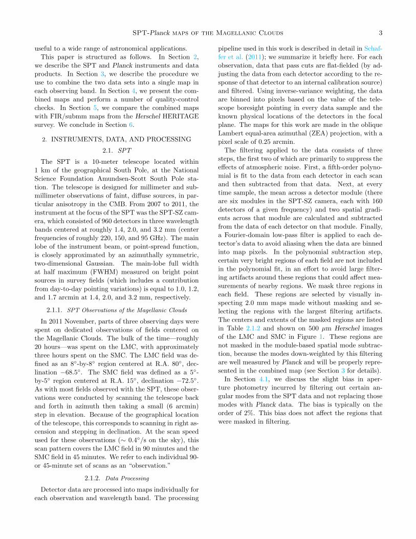
surements of nearby regions. We mask three regions in

each field. These regions are selected by visually in-

specting 2.0 mm maps made without masking and se-

lecting the regions with the largest filtering artifacts.

The centers and extents of the masked regions are listed

in Table 2.1.2 and shown on 500 µm Herschel images

of the LMC and SMC in Figure 1. These regions are

not masked in the module-based spatial mode subtrac-

tion, because the modes down-weighted by this filtering

are well measured by Planck and will be properly repre-

sented in the combined map (see Section 3 for details).

In Section 4.1, we discuss the slight bias in aper-

ture photometry incurred by filtering out certain an-

gular modes from the SPT data and not replacing those

modes with Planck data. The bias is typically on the

order of 2%. This bias does not affect the regions that

were masked in filtering.

4 Crawford et al.

Table 1. Regions masked in the SPT time-ordered data polynomial

subtraction

Field Mask center R.A. Mask center decl. Mask radius

[deg.] [deg.] [arcmin]

LMC 84.684 -69.105 20

LMC 74.265 -66.437 10

LMC 84.991 -69.682 10

SMC 15.414 -72.127 20

SMC 11.995 -73.105 10

SMC 18.635 -73.304 10

The individual-observation maps in each observing

band are combined into full coadded maps using inverse-

variance weighting. If the data from one observing band

in one individual observation has too few detectors that

pass cuts, or if any obvious artifacts are seen when the

single-observation map is visually inspected, the map

from that observation is not included in the coadded

map. Of the 14 individual LMC field observations, 10

are used in the 1.4 mm coadd, 12 in the 2.0 mm coadd,

and 12 in the 3.2 mm coadd. Of the four individual SMC

field observations, three are used in the 1.4 mm coadd

and all four at 2.0 and 3.2 mm. The most common

reason for detectors failing cuts is poor weather, which

affects the shorter wavelengths more severely (because

of the spectral dependence of atmospheric noise at mil-

limeter wavelengths—see, e.g., Bussmann et al. 2005).

In addition to the coadded signal maps, we create

coadded null maps for each observing band and field.

We combine these maps with Planck HFI null maps in

the same way as signal maps are combined, such that

the combined null maps can be used in estimating the

noise contribution to the uncertainty on any quantity

estimated from the combined signal maps. For SPT, we

create null maps by subtracting maps made from data in

right-going telescope scans only from maps made from

data in left-going telescope scans only (divided by two).

Any true sky signal should difference away in this opera-

tion, leaving an estimate of the instrumental and atmo-

spheric noise. The individual-observation null maps are

combined in the same way as the individual-observation

signal maps, except that an additional layer of differ-

encing is performed by multiplying one half of the ob-

servations by -1. Despite this double differencing (left

minus right, multiplying half the individual-observation

maps by -1), some small artifacts are visible in the null

maps at the location of the brightest regions of the two

fields—most notably at the location of 30 Doradus in

the LMC. These are due to slight differences in weights

Figure 1. Regions masked in the filtering of SPT time-ordered data. Top panel: 500 µm map of the LMC fromthe Herschel HERITAGE survey with the three masked LMCregions indicated by dashed circles (see Table 2.1.2 for exactlocations). Bottom panel: 500 µm map of the SMC fromthe Herschel HERITAGE survey with the three masked SMCregions indicated by dashed circles (see Table 2.1.2 for exactlocations).

and filtering in the left-going and right-going maps, and

the amplitude of the artifacts are at most 1% of the

amplitude of the original features.

2.1.3. Angular Response Function

As mentioned above, the true instrument beam in each

SPT observing band—i.e., the response to a point source

as a function of angular offset from the source that would

be measured in the absence of any processing to the

data—is well-approximated by an azimuthally symmet-

ric Gaussian. These beams are estimated from a combi-

nation of dedicated observations of planets and measure-

SPT-Planck maps of the Magellanic Clouds 5

ments of bright point sources in the SPT-SZ survey field

(for details, see Schaffer et al. 2011). The effect of the

filtering of SPT data is to modify this angular response

function—i.e., to alter the effective instrument beam.

Each filtering step has a specific impact on the effec-

tive beam. The polynomial subtraction imparts slight

negative lobes to the beam in the scan direction—in

this case R.A. or x—while the module-based filtering

imparts an isotropic negative ring at roughly half the

scale of a module, or ∼ 10 arcmin. The anti-aliasing

filter smooths the data in the scan direction at or just

above the pixel scale (0.25 arcmin); this smoothing is

negligible compared to the size of the true beam. All

of these effects are represented more cleanly in the two-

dimensional Fourier domain, and we use Fourier meth-

ods to estimate and represent the response function in

this work.

The filter response function is estimated using sim-

ulated observations. One hundred independent simu-

lated skies are created, in which the sky signal is white

noise convolved with a Gaussian with FWHM equal to

0.75 arcmin. For each simulated sky, a simulated version

of the full time-ordered data in each real observation of

the LMC or SMC field is created using the telescope

pointing and detector focal plane locations. These sim-

ulated time-ordered data are then filtered and made into

a map in the same manner as is used for the real data,

including detector cuts and weighting. The individual-

observation maps are combined into full coadded maps

using the same procedure and weighting as for the real

data. For each of the 100 simulated skies, the square of

the two-dimensional Fourier transform of the coadded

map is divided by the known input (2d) power spec-

trum. These 100 estimates are averaged, and the square

root of the result is our estimate of the 2d filter response

function. We multiply this (in Fourier space) by the

instrument beam to create the full beam-plus-filtering

response function.

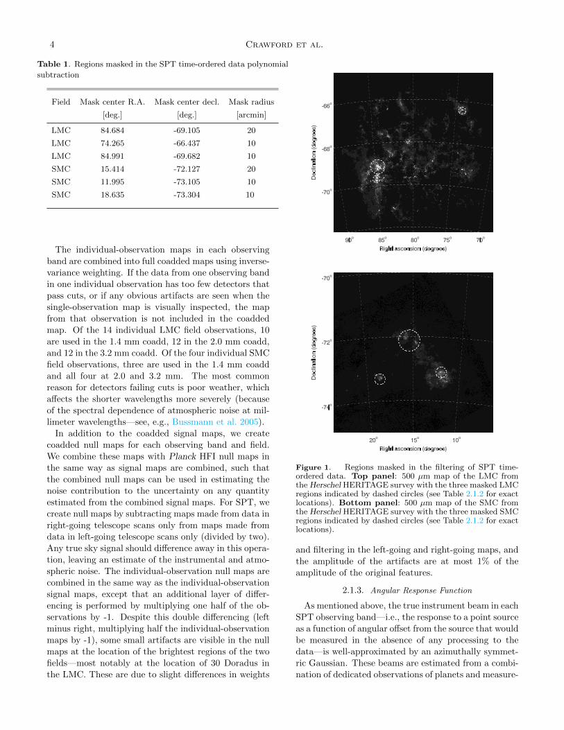
Figure 2 shows the full two-dimensional Fourier-

domain angular response function (beam plus filtering)

for the 2.0 mm SPT data used in this work. The filter

part of the response functions for the 1.4 and 3.2 mm

data are nearly identical to the filter part of the 2.0 mm

response function. The effect of each filtering step is con-

fined to a specific region of 2d Fourier space. The poly-

nomial subtraction acts as a one-dimensional high-pass

filter, suppressing modes at kx < 100, while the module-

based filter acts as an isotropic high-pass, suppressing

modes at k < 1000, where k is angular wavenumber

(k(λ) = 2π/λ for wavelength λ in radians), and kx is

the Fourier conjugate of the scan direction. The anti-

aliasing filter acts as a scan-direction low-pass filter with

a cutoff at kx ' 20,000; however the effect of this low-

pass is dominated by the isotropic low-pass of the in-

Figure 2. Two-dimensional Fourier-domain angular re-sponse function for the 2.0 mm SPT data used in this work.The response function is the product of the instrument beamor point-spread function and the filtering performed on thedata. The isotropic suppression of power at kx ' ky ' 0is from the subtraction of a common mode and two slopesacross each detector module at each time sample. The thinline of zero power along kx = 0 is from the subtraction of afifth-order polynomial from the data from each detector in-dividually on each scan across the field. The isotropic rolloffat high k is due to the beam.

strument beam and is not visible in Figure 2.

Finally, we note that the clean representation of the

filter response function in 2d Fourier space is to some

degree dependent on the projection used to map the

curved sky onto a flat, 2d grid. In particular, any filter-

ing that acts on single-detector time-ordered data will

result in an effective map-space filter along the scan di-

rection on the sky. Any projection in which the scan

direction (R.A.) corresponds to the x axis of the 2d map

will localize this filtering in 2d Fourier space to a partic-

ular region of 1d angular frequency or wavenumber kx.

This makes it easy to identify which Fourier modes in

the map have been downweighted by the filtering and to

replace those modes with modes from the correspond-

ing Planck HFI map. The downside of such a projec-

tion is that the mapping of R.A. to x everywhere in the

map necessarily leads to angular distortions at the map

edges. Such a projection is not optimal for representing

the true instrument beam in 2d Fourier space; an angle-

preserving projection such as the ZEA projection is more

appropriate for dealing with the beam. The maps used

6 Crawford et al.

to create the representation of the filter function in Fig-

ure 2 were made in a simple Cartesian projection, but

all other maps in this analysis are made in the ZEA

projection.

2.1.4. Noise Estimation

To combine SPT data with Planck HFI data in a

nearly optimal way, we need a measure of not only the

angular response function for each instrument but also

a measure of the noise in each data set. For SPT, the

noise is most cleanly represented in the two-dimensional

Fourier domain (as was the case with the SPT angu-

lar response function). We estimate the 2d noise power

spectrum by coadding the single-observation maps with

half the maps multiplied by -1, taking the Fourier trans-

form of the result and squaring, and repeating many

times with the negative sign assigned to a different set

of single-observation maps each time. For the SMC

field, there are not enough single-observation maps to

get a good noise estimate with this technique, so we use

the LMC field estimate scaled by the ratio of observing

depth for our SMC field estimate. We note that using

a single 2d Fourier estimate for the noise over an entire

field assumes that the noise properties are uniform over

the field. This is a very good approximation for the SPT

maps in this work, except for small regions at the edges

of the fields which are not used in the combination with

Planck HFI data.

2.1.5. Filter Deconvolution

In preparation for combining the SPT maps with

Planck HFI maps, we deconvolve the filter angular re-

sponse function from the maps, and we modify the noise

estimates to account for this deconvolution. We perform

this deconvolution in 2d Fourier space: after first multi-

plying the map by a real-space apodization window, we

Fourier transform the map, multiply in Fourier space

by the reciprocal of the filter response function, and in-

verse Fourier transform. To avoid numerical issues, we

set the reciprocal of the filter response to zero in any

region of 2d Fourier space in which the filter response is

less than 0.01. This conditioning step is taken into ac-

count when we combine the SPT and Planck maps. We

account for the deconvolution in the SPT noise estimates

by multiplying the 2d Fourier-space noise estimates by

the (conditioned) reciprocal of the filter response.

Note that we only deconvolve the azimuthally sym-

metric, low-k part of the filter response (the part of

Fourier space in which the data can be adequately re-

placed with Planck data) while leaving the low-kx, high-

ky part of the response function in the map. This means

that in the final, combined maps, a small fraction of an-

gular modes will be missing from the data (except in the

regions which were masked during this filtering step). As

can be seen from Figures 2 and 5, after combining with

Planck data, modes will be missing from a small area at

kx . 100 and ky & 2000. See Section 4.1 for a discussion

of the effects of ignoring this small fraction of missing

data in the final maps.

2.1.6. Astrometry Check

As discussed in detail in Schaffer et al. (2011), the re-

construction of the pointing (the instantaneous sky loca-

tion viewed by every detector at every time sample) for

the SPT is based on daily measurements of the Galac-

tic HII regions RCW38 and Mat5a, supplemented with

information from thermal, linear displacement, and tilt

sensors in the telescope. The typical precision in this

reconstruction is 7 arcsec (as measured by the rms vari-

ation in bright source positions over many individual ob-

servations of a field). The overall astrometric solution

for SPT maps is refined by comparing to source positions

in the Australia Telescope 20 GHz Survey (AT20G) cat-

alog (Murphy et al. 2010), which are tied to very long-

baseline interferometry calibrators and are accurate at

the 1-arcsec level. When we apply this technique to the

LMC and SMC fields, we find small (10-15 arcsec) but

statistically significant offsets between the original SPT

positions and the AT20G positions. We correct these

offsets by simply redefining the map centers. The final

map centers (which we use to reproject Planck data onto

the SPT grid and which we publish in the final combined

map FITS files) are R.A. 79.9906, decl. −68.4984 for

the LMC and R.A. 14.9849, decl. −72.4994 for the

SMC. Based on the analysis in Schaffer et al. (2011) we

expect that, after this correction, the astrometry is good

to roughly 2 arcsec rms.

2.2. Planck

The primary science goal of the Planck satellite

(Planck Collaboration et al. 2014a), launched in 2009

by the European Space Agency, was to map the CMB

over the full sky in nine bands, ranging in wavelength

from 350 µm to 1 cm. In this work, we use publicly

available Planck data in the three wavelength bands

that closely overlap with the three SPT bands. These

are three longest-wavelength or lowest-frequency bands

on the Planck High-Frequency Instrument (HFI) and

have nominal center wavelengths of 1.4, 2.1, and 3.0 mm

(nominal center frequencies of 217, 143, and 100 GHz).

The instrument beam or point-spread function in these

three bands is close to Gaussian and azimuthally sym-

metric, with FWHM equal to 5.0, 7.1, and 10.0 arcmin

at 1.4, 2.1, and 3.0 mm, respectively.

The Planck HFI time-ordered data are combined into

maps using an approximation to the minimum-variance

solution (Planck HFI Core Team et al. 2011), in con-

trast to the technique of filtering and naive bin-and-

SPT-Planck maps of the Magellanic Clouds 7

averaging used to make the SPT maps. This results in

maps that are unbiased estimates of the true sky signal

at all scales except for the effect of the instrument beam

and pixelization, and the DC component of the maps,

which is set to zero in the HFI mapmaking procedure

(Planck Collaboration et al. 2014b; for more discussion

of the zero-point treatment, see Section 3.4). Thus, the

angular response functions appropriate for the Planck

HFI maps are simply the convolution (or Fourier-space

product) of the instrument beams and the known pixel

window function. For more details on the Planck HFI

instrument and data, see Lamarre et al. (2010), Planck

Collaboration et al. (2014c), and Planck Collaboration

et al. (2016a).

To create Planck HFI maps of the Magellanic Clouds

that match the SPT maps described in the previ-

ous section, we first take the publicly available full-

mission maps4 in each of the three bands and resample

them from their native pixelization onto the 0.25-arcmin

oblique Lambert equal-area azimuthal (ZEA) projection

used for the SPT maps. For the R.A./decl. center of the

target projection, we use the center of the SPT maps de-

rived from the astrometry cross-check with the AT20G

survey (see Section 2.1.6 for details). The HFI maps are

stored using the full-sky HEALPix5 pixelization scheme,

with the HEALPix Nside parameter set to 2048, leading

to 12× 20482 pixels over the full sky, or a pixel scale of

1.7 arcmin. In the resampling to the 0.25-arcmin flat-sky

grid, we oversample each 0.25-arcmin pixel by a factor

of four to reduce the effect of resampling artifacts.

The Planck maps in the ZEA projection are then

matched to the resolution of the SPT maps by divid-

ing the Planck maps in 2d Fourier space by the ratio

of the Planck beam to the SPT beam in the closest ob-

serving band. The Planck beams used in this operation

are the product of the publicly available measured in-

strument beams and the HEALPix Nside = 2048 pixel

window function. This Fourier-space operation is equiv-

alent to deconvolving the Planck beam from the map

and convolving the result with the corresponding SPT

beam. At small enough scales (high enough wavenum-

ber k), this ratio becomes small enough to cause numer-

ical issues—and becomes increasingly uncertain as the

fractional Planck beam uncertainties grow larger—so we

artificially roll off the ratio at low values of the Planck

beam (B(k) < 0.005). This roll-off is taken into account

when we combine the SPT and Planck maps (see Section

3.3 for details).

4 Downloaded from the NASA/IPAC Infrared ScienceArchive: http://irsa.ipac.caltech.edu/data/Planck/release_2/all-sky-maps.

5 http://healpix.sourceforge.net

We also create null Planck HFI maps—using the pub-

licly available Planck half-mission maps—to combine

with the null SPT maps described in Section 2.1.2. We

make the null Planck maps by subtracting one half-

mission map from the other half-mission map (divided

by two) in each band, then resampling to the ZEA pro-

jection, and deconvolving the Planck-SPT beam ratio,

as done for the signal maps. As was the case in the SPT

null maps, there are small artifacts in the Planck null

maps at the location of the brightest regions of the two

fields, and, as with the SPT null maps, the artifacts are

at the percent level or below.

To combine these Planck HFI maps with the SPT

maps described in Section 2.1, we need an estimate of

the noise properties of the SPT-beam-matched Planck

maps. The noise in Planck HFI maps is uncorrelated

between pixels (white) to a very good approximation

(Planck HFI Core Team et al. 2011), so the Fourier-

domain Planck map noise in a uniform-coverage region

is well approximated by a single value at all k values or

angular scales. Thus, the Fourier-domain map noise in

one of the SPT-beam-matched Planck maps is this value

divided by the ratio of the Planck and SPT beams, un-

der the assumption that the Planck noise is uniform over

the map.

The Planck coverage in the SMC field is quite uniform,

only varying by ±12% across the field (corresponding to

±6% variations in noise). The LMC field is near the

south ecliptic pole, and the Planck observing strategy

results in regions of very high coverage near the ecliptic

poles. Approximately 25% of pixels in the LMC field are

in such a region (defined as 50% higher coverage than

the mode of the distribution in the rest of the field).

Using a single value for the noise across the field will

result in a slightly suboptimal combination of SPT and

Planck data for the high-weight regions. No bias results

from this approximation, and the variation of Planck

noise across the field will be properly represented in the

combined SPT+Planck null maps. For both fields, we

estimate the Planck noise by taking the square root of

the mean of the variance values for all pixels in the region

covered by SPT. The pixel variance values are provided

by the Planck team in the same files as the maps.

3. COMBINING DATA FROM SPT AND PLANCK

There are two main steps in the process of optimally

combining the SPT and Planck maps described in pre-

vious sections. First, the maps are relatively calibrated

(or, more specifically, the SPT map is adjusted to match

the Planck maps) and converted from CMB fluctuation

temperature to brightness or specific intensity (in units

of MJy sr−1) at a fiducial observing wavelength and for

an assumed source spectrum. Then the maps from the

two instruments are combined into a single map using

8 Crawford et al.

inverse-variance weights calculated from the noise esti-

mate for each instrument in each field and band. Each

of these steps is described in greater detail below.

3.1. Absolute Calibration

Before the SPT and Planck HFI data can be mean-

ingfully combined into a single map, care must be

taken to ensure that the two data sets are consistently

calibrated—that is, that a true sky signal would pro-

duce the same amplitude of response in both data sets

(up to differences in the angular response function of

the two instruments). Maps from both instruments are

stored in units of CMB fluctuation temperature, i.e.,

the variation in temperature of a blackbody with mean

temperature 2.73K that would produce the detected sig-

nal. The absolute calibration of the Planck maps used

in this work is taken from the annual modulation of the

CMB dipole due to the motion of the satellite around

the solar system barycenter (Planck Collaboration et al.

2016a). The fractional statistical uncertainty on this cal-

ibration is significantly less than 1%. This calibration

can be checked by comparing the CMB power spectrum

measured with Planck to the CMB power spectrum mea-

sured by the WMAP team, who also calibrate their data

off of the modulation of the CMB dipole, using inter-

nal WMAP measurements. The CMB power spectrum

measurements from the two instruments agree to better

than 1% in power (0.5% in CMB fluctuation tempera-

ture, Planck Collaboration et al. 2016b).

The SPT absolute calibration is obtained by match-

ing the small-scale (high-multipole) CMB power spec-

trum measured with SPT and published in George et al.

(2015) with the Planck CMB power spectrum over the

same multipole range (670 < ` < 1170, where ` is multi-

pole number and, over small patches of sky, is equivalent

to angular wavenumber k as defined in Section 2.1.3).The fractional statistical uncertainty on this calibration

is roughly 2.5% (in temperature) at 1.4 mm and 1.0%

(in temperature) at 2.0 and 3.2 mm.

3.2. Spectral Matching

As discussed in the previous section, the absolute cal-

ibration of both the SPT and Planck data used here

is based on a source with an emission spectrum de-

scribed by fluctuations around a 2.73K blackbody, i.e.,

I(λ) ∝ dB/dT (λ, 2.73K), where B(λ, T ) is the Planck

blackbody function. If the SPT and Planck bands were

infinitely narrow, or if they had finite width but were

identical in response as a function of wavelength (or

bandpass), the calibration step described above would

be sufficient for matching the SPT and Planck maps of

a source with an arbitrary emission spectrum. In reality,

the SPT and Planck bands have fractional widths of or-

der 30%, and there are small but significant differences

Figure 3. Bandpass functions, or instrument response asa function of wavelength, for SPT-SZ and the lowest threebands of Planck HFI. Planck bands are shown by the solidblack lines, while SPT-SZ bands are shown by the dashedred lines. The normalization of the bandpasses is arbitrary.

in the bandpass functions for the two instruments, as

shown in Figure 3. (The publicly available Planck bands

were downloaded from the same server as the maps and

instrument beams.)

Because of this small bandpass mismatch, and because

the emission from the Magellanic Clouds is not expected

to have a dB/dT (λ, 2.73K) spectrum, we need to apply

some further correction factor to match the SPT and

Planck responses to the emission from the Magellanic

Clouds. The size of that correction depends on the spec-

tral energy distributions (SEDs) at each point within

the LMC and SMC and the different SPT and Planck

bandpass functions. To choose the appropriate spectral

matching factor, we need some prior information on the

SEDs of the Magellanic Clouds. Fortunately, the SEDs

can be approximated by power laws with a limited range

of index. In the following section, we use Planck data in

the bands under investigation here and in the neighbor-

ing HFI bands to estimate the SEDs of the LMC and

SMC at the angular scales accessible to Planck.

3.2.1. Spectral Energy Distributions of the MagellanicClouds from Planck-only Data.

In this section, we use Planck data from 0.85 mm to

4.3 mm to estimate the SEDs of the LMC and SMC at

Planck angular scales. One complication to this pro-

cess is evident from Planck-only maps of the Magellanic

Clouds in Figure 1 of Planck Collaboration et al. (2011).

For example, in the LMC, the dust emission (traced by

the 0.35 mm or 857 GHz map) is quite diffuse and covers

the entire region, while the synchrotron emission (traced

by the 10.5 mm or 28.5 GHz map) is concentrated in

bright regions such as 30 Doradus. This makes it un-

likely that a single SED will be sufficient to describe the

SPT-Planck maps of the Magellanic Clouds 9

(a) LMC (b) SMC

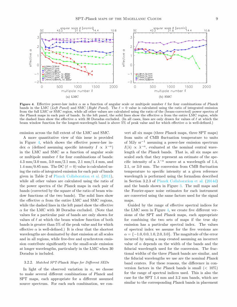
Figure 4. Effective power-law index α as a function of angular scale or multipole number ` for four combinations of Planckbands in the LMC (Left Panel) and SMC (Right Panel). The ` = 0 value is calculated using the ratio of integrated emissionfrom the full LMC or SMC region, while all other values are calculated using the ratio of the (beam-corrected) power spectra ofthe Planck maps in each pair of bands. In the left panel, the solid lines show the effective α from the entire LMC region, whilethe dashed lines show the effective α with 30 Doradus excluded. (In all cases, lines are only drawn for values of ` at which thebeam window function for the longest-wavelength band is above 5% of peak value and for which effective α is well-defined.)

emission across the full extent of the LMC and SMC.

A more quantitative view of this issue is provided

in Figure 4, which shows the effective power-law in-

dex α (defined assuming specific intensity I ∝ λ−α)

in the LMC and SMC as a function of angular scale

or multipole number ` for four combinations of bands:

4.3 mm/3.0 mm, 3.0 mm/2.1 mm, 2.1 mm/1.4 mm, and

1.4 mm/0.85 mm. The DC (` = 0) value is calculated us-

ing the ratio of integrated emission for each pair of bands

given in Table 2 of Planck Collaboration et al. (2011),

while all other values are calculated using the ratio of

the power spectra of the Planck maps in each pair of

bands (corrected by the square of the ratio of beam win-

dow functions of the two bands). The solid lines show

the effective α from the entire LMC and SMC regions,

while the dashed lines in the left panel show the effective

α for the LMC with 30 Doradus excluded. (Note that

values for a particular pair of bands are only shown for

values of ` at which the beam window function of both

bands is greater than 5% of the peak value and for which

effective α is well-defined.) It is clear that the shortest

wavelengths are dominated by dust emission at all scales

and in all regions, while free-free and synchrotron emis-

sion contribute significantly to the small-scale emission

at longer wavelengths, particularly in the LMC when 30

Doradus is included.

3.2.2. Matched SPT-Planck Maps for Different SEDs

In light of the observed variation in α, we choose

to make several different combinations of Planck and

SPT maps, each appropriate for a different assumed

source spectrum. For each such combination, we con-

vert all six maps (three Planck maps, three SPT maps)

from units of CMB fluctuation temperature to units

of MJy sr−1 assuming a power-law emission spectrum

I(λ) ∝ λ−α, evaluated at the nominal central wave-

length of the Planck bands. That is, all six maps are

scaled such that they represent an estimate of the spe-

cific intensity of a λ−α source at a wavelength of 1.4,

2.1, or 3.0 mm. The conversion from CMB fluctuation

temperature to specific intensity at a given reference

wavelength is performed using the formalism described

in Section 3.2.3 of Planck Collaboration et al. (2014d)

and the bands shown in Figure 3. The null maps and

the Fourier-space noise estimates for each instrument

are converted using the same factors used for the signal

maps.

Guided by the range of effective spectral indices for

the LMC seen in Figure 4, we create five different ver-

sions of the SPT and Planck maps, each appropriate

for combining the two sets of maps if the true sky

emission has a particular spectral index. The values

of spectral index we assume for the five versions are

α = −1.0, 0.0, 1.0, 2.0, 3.0. The magnitude of the error

incurred by using a map created assuming an incorrect

value of α depends on the width of the bands and the

fiducial wavelength used for the conversion. The frac-

tional widths of the three Planck bands are similar, and

the fiducial wavelengths we use are the nominal Planck

band centers. For these reasons, the difference in con-

version factors in the Planck bands is small (< 10%)

for the range of spectral indices used. This is also the

case for the SPT 1.4 mm and 3.2 mm bands, which are

similar to the corresponding Planck bands in placement

10 Crawford et al.

and width. However, the SPT 2.0 mm band is signif-

icantly offset from the Planck 2.1 mm band, and the

factors to convert data in that band from CMB fluctu-

ation temperature to MJy sr−1 at the nominal Planck

band center vary by 30% between α = −1 and α = 3.

This is the strongest motivation for creating multiple

sets of combined maps. If a user of the final data prod-

ucts needs a map appropriate for a non-integer spectral

index (or an index outside the range we use) and de-

sires conversion accuracy better than 5% (roughly the

difference between the SPT 2.0 mm conversion factors

assuming α = α0 and assuming α = α0± 1), we suggest

interpolating between maps or extrapolating.

3.2.3. Beam-filling vs. Point-like Sources

A further complication to the calculation of conver-

sion factors between CMB temperature and MJy sr−1 is

the question of beam-filling vs. point-like sources. For

diffraction-limited optical systems that couple to a sin-

gle mode of radiation per polarization, the product of

telescope area and beam solid angle (AΩ or etendue)

is equal to λ2. Both SPT and Planck operate in or

near this single-moded, diffraction limit for the bands

considered here (Padin et al. 2008; Ade et al. 2010).

In the limit of constant telescope aperture illumination

as a function of wavelength, the AΩ from a point-like

source will be constant, while the AΩ for a beam-filling

source will go as λ2. The power received by an opti-

cal system from a source scales directly with AΩ, so in

this limit the conversion factor calculated for a point

source with spectral index α will be equivalent to the

conversion factor for a beam-filling source with spectral

index α + 2. For the reasons discussed above, this dis-

tinction matters significantly only for the SPT 2.0 mm

band, where it is up to a 15% difference. All the con-

version factors we use here assume beam-filling sources,

mainly because that is how the bands and absolute cal-

ibration were measured for both instruments (Schaffer

et al. 2011; Planck Collaboration et al. 2014d). There

are few isolated features at sub-arcminute scales in the

Magellanic Clouds (e.g., Meixner et al. 2013, Figure 14),

so this is a safe choice for the SPT bands; the assumption

is less safe for Planck, but the differences between beam-

filling and point-source conversion factors for Planck are

much smaller (at the percent level).

3.3. Combining Maps Using Inverse-variance

Weighting

Once the SPT and Planck maps are in a common set

of units and are consistently calibrated, and we have es-

timates of the noise for both maps, it is straightforward

to combine them in an optimal (minimum-variance) way

using inverse-variance weights. The noise estimates are

not perfect, and the combined maps are thus not truly

optimal. The degree to which the combined maps are

sub-optimal depends on the fidelity of the noise esti-

mates and the assumptions underlying these estimates,

particularly that of uniform noise across the entire map.

As discussed in previous sections, the SPT noise prop-

erties are very uniform across the map in both the LMC

and SMC fields, while the Planck noise properties are

very uniform in the SMC map but not in the LMC

map. (A fraction of the pixels in the LMC have Planck

noise that is significantly lower than the mean.) The

SPT-Planck combination will be slightly sub-optimal for

these map regions, but there is no signal bias; further-

more, the combined SPT-Planck null maps properly re-

flect this variation in noise in the LMC field.

To combine the maps in a given band, we first Fourier

transform each map. At each point in 2d Fourier space

k = [kx, ky], we define a weight for each map

W (k) = N−2(k), (1)

where N(k) is the Fourier-space noise estimate. Re-

call that for Planck we assume white noise in the raw

maps, so that the Fourier-space noise in the SPT-beam-

matched maps will be proportional to the ratio of the

beams:

NPlanck(k) ∝ BSPT(k)/BPlanck(k). (2)

This ratio is a monotonically increasing function of k

and reaches a value of 10 at approximately k = 3700 at

1.4 mm, k = 2500 at 2.1 mm, and k = 1900 at 3.0 mm.

Hence, the Planck weights will be down by a factor of

100 at these k values compared to k = 0. Meanwhile,

the SPT maps have had the filter response function de-

convolved, so the noise in these maps is given by

NSPT(k) = NSPT,orig(k)/FSPT(k), (3)

where NSPT,orig(k) is the estimate of the noise from theoriginal maps, and FSPT(k) is the SPT filter response

function. From this it is clear that the Planck weights

will be proportional to the square of the ratio of the

Planck beam to the SPT beam, while the SPT weights

will be reasonably flat (depending on the noise prop-

erties in the original maps) except for the regions of

Fourier space strongly affected by the filtering, which

will have much lower weight. We manually zero the

Planck weights at any values of k at which the value of

the Planck beam is lower than 0.005, and we manually

zero the SPT weights at values of k at which the az-

imuthally symmetric part of the SPT filter response is

less than 0.01.

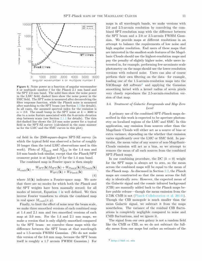
The azimuthally averaged values of N2Planck(∝

W−1Planck) and N2

SPT(∝W−1SPT) as a function of k in both

fields are shown for the 2.1/2.0 mm bands and an as-

sumed spectral index α = 2.0 in Figure 5. For com-

parison, we also show N2SPT at 2.0 mm from a typi-

SPT-Planck maps of the Magellanic Clouds 11

Figure 5. Noise power as a function of angular wavenumberk or multipole number ` for the Planck 2.1 mm band andthe SPT 2.0 mm band. The solid lines show the noise powerin the LMC field; dashed lines show the noise power in theSMC field. The SPT noise is measured after deconvolving thefilter response function, while the Planck noise is measuredafter matching to the SPT beam (see Section 3.3 for details).In all cases, the assumed spectral index for the emission isα = 2.0. The small bump in the SPT noise at k = 3600 isdue to a noise feature associated with the 6-arcmin elevationstep between scans (see Section 2.1.1 for details). The thindot-dashed line shows the 2.0 mm noise power for a typicalfield in the SPT-SZ survey (calculated in the same manneras for the LMC and the SMC curves in this plot).

cal field in the 2500-square-degree SPT-SZ survey (in

which the typical field was observed a factor of roughly

10 longer than the total LMC observations used in this

work). Plots of N2Planck and N2

SPT in the 1.4 mm and

3.0 mm bands look similar, except that the Planck/SPT

crossover point is at higher k/` for the 1.4 mm band.

The combined map in Fourier space is then simply

Mcomb(k) =WSPT(k)MSPT(k) +WPlanck(k)MPlanck(k)

WSPT(k) +WPlanck(k),

(4)

where M(k) indicates a Fourier-space map. We note

that there are no modes for which both the Planck and

the SPT weights have been manually zeroed; for all

modes of interest, Equation 4 is well defined. We then

inverse Fourier transform to obtain the combined map

in real space Mcomb(x, y).

Finally, to limit the effect of noise near the beam scale,

we make three smoothed versions of each combined map

at 1.4 and 2.1 mm and two smoothed versions of each

map at 3.0 mm. For the 1.4 and 2.1 mm maps, we

make a version that is only slightly smoothed compared

to the SPT beam: we convolve these maps with the

difference between the SPT beam at that wavelength

and a 1.5-arcmin FWHM Gaussian. (We do not make

this version of the 3.0 mm map, because the SPT beam

itself is roughly a 1.7 arcmin FWHM Gaussian.) For

maps in all wavelength bands, we make versions with

2.0 and 2.5-arcmin resolution by convolving the com-

bined SPT-resolution map with the difference between

the SPT beam and a 2.0 or 2.5-arcmin FWHM Gaus-

sian. We provide maps at different resolutions in an

attempt to balance the requirements of low noise and

high angular resolution. End users of these maps that

are interested in the smallest-scale features of the Magel-

lanic Clouds should use the highest-resolution maps and

pay the penalty of slightly higher noise, while users in-

terested in, for example, performing few-arcminute scale

photometry on the maps should use the lower-resolution

versions with reduced noise. Users can also of course

perform their own filtering on the data—for example,

loading one of the 1.5-arcmin-resolution maps into the

SAOImage ds9 software6 and applying the Gaussian

smoothing kernel with a kernel radius of seven pixels

very closely reproduces the 2.5-arcmin-resolution ver-

sion of that map.

3.4. Treatment of Galactic Foregrounds and Map Zero

Level

A primary use of the combined SPT-Planck maps de-

scribed in this work is expected to be aperture photom-

etry on localized regions of the LMC and SMC. In this

application, any emission from sources other than the

Magellanic Clouds will either act as a source of bias or

extra variance, depending on the whether that emission

varies significantly over the LMC or SMC field. In par-

ticular, the mean value of any source of non-Magellanic-

Clouds emission will act as a bias, so we attempt to

remove the mean of all such sources from the combined

SPT-Planck maps.

In our combining procedure, the DC (k = 0) weight

for the SPT maps is always set to zero, so the mean

across the combined maps will be equal to the mean of

the Planck map. As discussed in Section 2.2, the Planck

maps are constructed so that the mean across the full

sky is identically zero. However, the expected mean of

the Galactic signal and the cosmic infrared background

(CIB) are manually added back to the Planck maps be-

fore public release—though the mean emission from the

2.73K CMB is not (Planck Collaboration et al. 2014b).

Though the CIB monopole is much smaller than the

mean Galactic signal, we subtract it from the maps

nonetheless. The variance of the residual CIB fluctu-

ations is completely negligible compared to noise and

CMB fluctuations, and we ignore it.

The signal from our own galaxy is not a random field

like the CMB or CIB, so we do not subtract the full-

sky mean from our maps but rather an estimate of the

6 http://ds9.si.edu

12 Crawford et al.

mean in the direction of the LMC or SMC. We esti-

mate this mean in each Planck band by taking the mean

signal quoted at 0.35 mm (857 GHz) in Planck Col-

laboration et al. (2011) toward each region and scal-

ing by the Galactic cirrus spectral energy distribution

quoted in Planck Collaboration et al. (2015). This as-

sumes the Galactic foreground signal is dust-dominated

across all the frequencies treated here, an assumption

supported by Figure 4 of Planck Collaboration et al.

(2011). The residual variance across the LMC and SMC

is estimated in Planck Collaboration et al. (2011) to be

10−3 MJy sr−1 rms in all bands and in both regions,

a factor of at least 10 below the CMB fluctuation level

(see Section 4.3.2), and we ignore this source of vari-

ance as well. The variance from CMB fluctuations is

discussed in detail in Section 4.3.2.

4. RESULTS

The primary result of this work consists of two sets

of 40 maps (one set each for the LMC and SMC fields).

These maps are 1800-by-1800 pixels and 1200-by-1200

pixels—or 7.5-by-7.5 degrees and 5-by-5 degrees—for

the LMC and SMC fields, respectively. Each set of

40 maps consists of eight maps each created assum-

ing one of five emission underlying spectra (power-

law emission I(λ) ∝ λ−α with spectral index α =

−1.0, 0.0, 1.0, 2.0, 3.0). For each value of spectral in-

dex, the eight maps consist of three maps of combined

SPT and Planck data at 1.4 mm (one each at resolutions

of 1.5, 2.0, and 2.5 arcmin), three maps of combined SPT

and Planck data at 2.1 mm (one each at resolutions of

1.5, 2.0, and 2.5 arcmin), and two maps of combined

SPT and Planck data at 3.0 mm (one each at resolu-

tions of 2.0, and 2.5 arcmin).

In this Section, we perform some simple tests to ver-

ify certain assumptions or expectations about the maps,in particular their resolution and their fidelity to the

original Planck data. These tests and the results are

discussed in Section 4.1. In Section 4.2, we show images

from a selection of maps, centered on certain features of

interest in the LMC and SMC, and discuss the proper-

ties of the maps evident from these images. Finally, we

discuss the instrumental and astrophysical noise prop-

erties of the maps in Section 4.3.

4.1. Combined Map Checks

In this section, we perform three checks on the com-

bined SPT+Planck maps and the process used to con-

struct them. First, we use simulated observations to

calculate the effect of ignoring the thin stripe of low-kx,

high-ky modes removed by the SPT scan-direction fil-

tering and not replaced with Planck data (see Section

2.1.5 for details). Next we verify the fidelity of the final,

combined maps by comparing them with the original

Planck data. Because of the nature of the SPT and

Planck data, in particular the filtering of large angu-

lar scales (low-k Fourier modes) from the SPT data (see

Section 3.3 for details), we expect the combined maps to

be dominated on large scales (small values of wavenum-

ber k) by the information from the Planck maps, and

we check that this expectation is borne out. Finally,

we confirm the expected angular response function of

the final, combined, Gaussian-smoothed maps: If our

measurements of the Planck and SPT beams and of the

SPT filter response are accurate, then we expect that

the only angular response function in the final maps is

the Gaussian smoothing (except for adjustments of the

overall mean intensity in the LMC or SMC region—see

Section 3.4 for details).

To estimate the bias that results from ignoring the

small fraction of Fourier modes removed from the SPT

maps and not replaced by Planck data, we create sim-

ulated maps with the same filtering as the real SPT

maps and combine them with simulated Planck maps of

the same mock skies. We then perform aperture pho-

tometry on the simulated combined SPT+Planck maps

and compare the results to aperture photometry on the

true, underlying mock skies. We create many mock skies

with features on different angular scales, and we per-

form aperture photometry using many different aperture

radii. For features on scales of 1 to 10 arcminutes and

aperture radii in the same range, we find a typical bias

of < 2% and a maximum bias of < 4% resulting from

the missing low-kx, high-ky modes.

We verify the fidelity to the original Planck maps in

two ways. First, in Figure 6 we show four versions of

the 2.1 mm, α = 2.0 map of the LMC field: 1) the

Planck data (not beam-matched to SPT) directly pro-

jected onto the final ZEA grid; 2) the filtered SPT data

projected onto the final ZEA grid; 3) the 1.5-arcmin-

FWHM version of the final map; 4) the map in (3) con-

volved with the difference between a 1.5-arcmin-FWHM

Gaussian and the Planck 2.1 mm beam. There is strong

visual agreement between the original Planck map and

the final maps smoothed to Planck resolution. To make

this more quantitative, we calculate the power spectrum

of each of these maps and plot these and the ratio be-

tween them in Figure 6. To avoid noise bias in the

power spectrum, we create two versions of each map

using only half the SPT or Planck data and calculate a

cross-spectrum between the two half-depth maps. We

mask the region around 30 Doradus before computing

the power spectrum, as it otherwise dominates the power

on all scales. As shown in Figure 6, the power spectrum

calcluated from these two maps agrees to better than

5% at all scales on which there is significant power in

the maps. These two results support the idea that these

maps are dominated by Planck information on scales

SPT-Planck maps of the Magellanic Clouds 13

(a) Planck-only, SPT-only, and Planck+SPT maps of the 7-by-7-degree LMC field

(b) Planck+SPT map matched to the original Planck resolution (Left Panel); power spectrum of thePlanck-only map and the Planck-matched combined map and their ratio (Right panel)

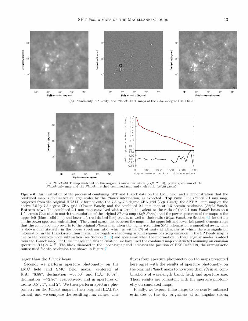
Figure 6. An illustration of the process of combining SPT and Planck data on the LMC field, and a demonstration that thecombined map is dominated at large scales by the Planck information, as expected. Top row: The Planck 2.1 mm map,projected from the original HEALPix format onto the 7.5-by-7.5-degree ZEA grid (Left Panel); the SPT 2.1 mm map on thenative 7.5-by-7.5-degree ZEA grid (Center Panel); and the combined 2.1 mm map at 1.5 arcmin resolution (Right Panel).Bottom row: The combined 2.1 mm map convolved with a kernel equivalent to the ratio of the 2.1 mm Planck beam to a1.5-arcmin Gaussian to match the resolution of the original Planck map (Left Panel); and the power spectrum of the maps in theupper left (black solid line) and lower left (red dashed line) panels, as well as their ratio (Right Panel, see Section 4.1 for detailson the power spectrum calculation). The visual agreement between the maps in the upper left and lower left panels demonstratesthat the combined map reverts to the original Planck map when the higher-resolution SPT information is smoothed away. Thisis shown quantitatively in the power spectrum ratio, which is within 5% of unity at all scales at which there is significantinformation in the Planck-resolution maps. The negative shadowing around regions of strong emission in the SPT-only map isdue to the common-mode subtraction (see Section 2.1.3) and goes away when the information in these angular modes is addedfrom the Planck map. For these images and this calculation, we have used the combined map constructed assuming an emissionspectrum I(λ) ∝ λ−2. The black diamond in the upper-right panel indicates the position of PKS 0437-719, the extragalacticsource used for the resolution test shown in Figure 7.

larger than the Planck beam.

Second, we perform aperture photometry on the

LMC field and SMC field maps, centered at

R.A.=78.88, declination=−68.50 and R.A.=16.07,

declination=−72.86, respectively, and in apertures of

radius 0.5, 1, and 2. We then perform aperture pho-

tometry on the Planck maps in their original HEALPix

format, and we compare the resulting flux values. The

fluxes from aperture photometry on the maps presented

here agree with the results of aperture photometry on

the original Planck maps to no worse than 2% in all com-

binations of wavelength band, field, and aperture size.

These results are consistent with the aperture photom-

etry on simulated maps.

Finally, we expect these maps to be nearly unbiased

estimates of the sky brightness at all angular scales;

14 Crawford et al.

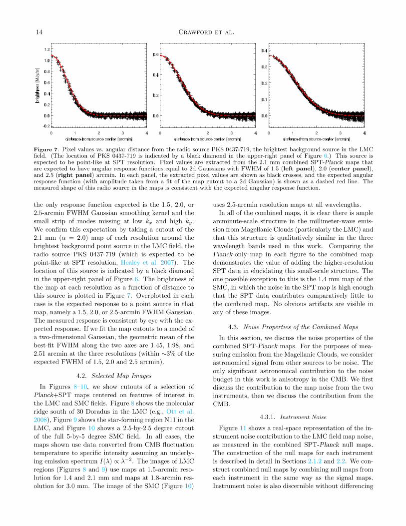
Figure 7. Pixel values vs. angular distance from the radio source PKS 0437-719, the brightest background source in the LMCfield. (The location of PKS 0437-719 is indicated by a black diamond in the upper-right panel of Figure 6.) This source isexpected to be point-like at SPT resolution. Pixel values are extracted from the 2.1 mm combined SPT-Planck maps thatare expected to have angular response functions equal to 2d Gaussians with FWHM of 1.5 (left panel), 2.0 (center panel),and 2.5 (right panel) arcmin. In each panel, the extracted pixel values are shown as black crosses, and the expected angularresponse function (with amplitude taken from a fit of the map cutout to a 2d Gaussian) is shown as a dashed red line. Themeasured shape of this radio source in the maps is consistent with the expected angular response function.

the only response function expected is the 1.5, 2.0, or

2.5-arcmin FWHM Gaussian smoothing kernel and the

small strip of modes missing at low kx and high ky.

We confirm this expectation by taking a cutout of the

2.1 mm (α = 2.0) map of each resolution around the

brightest background point source in the LMC field, the

radio source PKS 0437-719 (which is expected to be

point-like at SPT resolution, Healey et al. 2007). The

location of this source is indicated by a black diamond

in the upper-right panel of Figure 6. The brightness of

the map at each resolution as a function of distance to

this source is plotted in Figure 7. Overplotted in each

case is the expected response to a point source in that

map, namely a 1.5, 2.0, or 2.5-arcmin FWHM Gaussian.

The measured response is consistent by eye with the ex-

pected response. If we fit the map cutouts to a model of

a two-dimensional Gaussian, the geometric mean of the

best-fit FWHM along the two axes are 1.45, 1.98, and

2.51 arcmin at the three resolutions (within ∼3% of the

expected FWHM of 1.5, 2.0 and 2.5 arcmin).

4.2. Selected Map Images

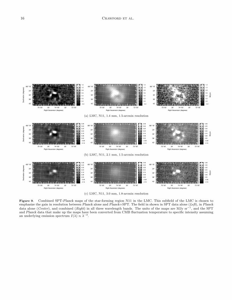
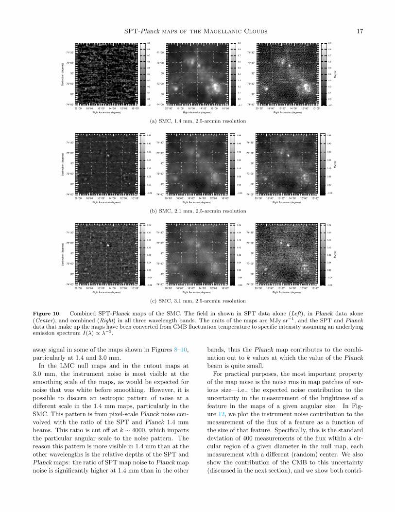
In Figures 8–10, we show cutouts of a selection of

Planck+SPT maps centered on features of interest in

the LMC and SMC fields. Figure 8 shows the molecular

ridge south of 30 Doradus in the LMC (e.g., Ott et al.

2008), Figure 9 shows the star-forming region N11 in the

LMC, and Figure 10 shows a 2.5-by-2.5 degree cutout

of the full 5-by-5 degree SMC field. In all cases, the

maps shown use data converted from CMB fluctuation

temperature to specific intensity assuming an underly-

ing emission spectrum I(λ) ∝ λ−2. The images of LMC

regions (Figures 8 and 9) use maps at 1.5-arcmin reso-

lution for 1.4 and 2.1 mm and maps at 1.8-arcmin res-

olution for 3.0 mm. The image of the SMC (Figure 10)

uses 2.5-arcmin resolution maps at all wavelengths.

In all of the combined maps, it is clear there is ample

arcminute-scale structure in the millimeter-wave emis-

sion from Magellanic Clouds (particularly the LMC) and

that this structure is qualitatively similar in the three

wavelength bands used in this work. Comparing the

Planck-only map in each figure to the combined map

demonstrates the value of adding the higher-resolution

SPT data in elucidating this small-scale structure. The

one possible exception to this is the 1.4 mm map of the

SMC, in which the noise in the SPT map is high enough

that the SPT data contributes comparatively little to

the combined map. No obvious artifacts are visible in

any of these images.

4.3. Noise Properties of the Combined Maps

In this section, we discuss the noise properties of the

combined SPT-Planck maps. For the purposes of mea-

suring emission from the Magellanic Clouds, we consider

astronomical signal from other sources to be noise. The

only significant astronomical contribution to the noise

budget in this work is anisotropy in the CMB. We first

discuss the contribution to the map noise from the two

instruments, then we discuss the contribution from the

CMB.

4.3.1. Instrument Noise

Figure 11 shows a real-space representation of the in-

strument noise contribution to the LMC field map noise,

as measured in the combined SPT-Planck null maps.

The construction of the null maps for each instrument

is described in detail in Sections 2.1.2 and 2.2. We con-

struct combined null maps by combining null maps from

each instrument in the same way as the signal maps.

Instrument noise is also discernible without differencing

SPT-Planck maps of the Magellanic Clouds 15

84°00'85°00'86°00'87°00'Right Ascension (degrees)

30'

-71°00'

30'

-70°00'

-69°30'De

clina

tion

(deg

rees

)

−0.2

0.0

0.2

0.4

0.6

0.8

1.0

1.2

84°00'85°00'86°00'87°00'Right Ascension (degrees)

30'

-71°00'

30'

-70°00'

-69°30'

−0.2

0.0

0.2

0.4

0.6

0.8

1.0

1.2

84°00'85°00'86°00'87°00'Right Ascension (degrees)

30'

-71°00'

30'

-70°00'

-69°30'

−0.2

0.0

0.2

0.4

0.6

0.8

1.0

1.2

MJy

/sr

(a) LMC, molecular ridge below 30 Doradus, 1.4 mm, 1.5-arcmin resolution

84°00'85°00'86°00'87°00'Right Ascension (degrees)

30'

-71°00'

30'

-70°00'

-69°30'

Decli

natio

n (d

egre

es)

−0.16

−0.08

0.00

0.08

0.16

0.24

0.32

0.40

0.48

84°00'85°00'86°00'87°00'Right Ascension (degrees)

30'

-71°00'

30'

-70°00'

-69°30'

−0.16

−0.08

0.00

0.08

0.16

0.24

0.32

0.40

0.48

84°00'85°00'86°00'87°00'Right Ascension (degrees)

30'

-71°00'

30'

-70°00'

-69°30'

−0.16

−0.08

0.00

0.08

0.16

0.24

0.32

0.40

0.48

MJy

/sr

(b) LMC, molecular ridge below 30 Doradus, 2.1 mm, 1.5-arcmin resolution

84°00'85°00'86°00'87°00'Right Ascension (degrees)

30'

-71°00'

30'

-70°00'

-69°30'

Decli

natio

n (d

egre

es)

−0.16

−0.08

0.00

0.08

0.16

0.24

0.32

0.40

0.48

84°00'85°00'86°00'87°00'Right Ascension (degrees)

30'

-71°00'

30'

-70°00'

-69°30'

−0.16

−0.08

0.00

0.08

0.16

0.24

0.32

0.40

0.48

84°00'85°00'86°00'87°00'Right Ascension (degrees)

30'

-71°00'

30'

-70°00'

-69°30'

−0.16

−0.08

0.00

0.08

0.16

0.24

0.32

0.40

0.48

MJy

/sr

(c) LMC, molecular ridge below 30 Doradus, 3.0 mm, 1.8-arcmin resolution

Figure 8. Combined SPT-Planck maps of the molecular ridge below 30 Doradus in the LMC. This subfield of the LMC ischosen to emphasize the gain in resolution between Planck alone and Planck+SPT. The field in shown in SPT data alone (Left),in Planck data alone (Center), and combined (Right) in all three wavelength bands. The units of the maps are MJy sr−1, andthe SPT and Planck data that make up the maps have been converted from CMB fluctuation temperature to specific intensityassuming an underlying emission spectrum I(λ) ∝ λ−2.

16 Crawford et al.

73°00'30'74°00'30'75°00'Right Ascension (degrees)

42'

36'

30'

24'

-66°18'

Decli

natio

n (d

egre

es)

−0.2

0.0

0.2

0.4

0.6

0.8

1.0

1.2

73°00'30'74°00'30'75°00'Right Ascension (degrees)

42'

36'

30'

24'

-66°18'

−0.2

0.0

0.2

0.4

0.6

0.8

1.0

1.2

73°00'30'74°00'30'75°00'Right Ascension (degrees)

42'

36'

30'

24'

-66°18'

−0.2

0.0

0.2

0.4

0.6

0.8

1.0

1.2

MJy

/sr

(a) LMC, N11, 1.4 mm, 1.5-arcmin resolution

73°00'30'74°00'30'75°00'Right Ascension (degrees)

42'

36'

30'

24'

-66°18'

Decli

natio

n (d

egre

es)

−0.16−0.080.000.080.160.240.320.400.48

73°00'30'74°00'30'75°00'Right Ascension (degrees)

42'

36'

30'

24'

-66°18'

−0.16−0.080.000.080.160.240.320.400.48

73°00'30'74°00'30'75°00'Right Ascension (degrees)

42'

36'

30'

24'

-66°18'

−0.16−0.080.000.080.160.240.320.400.48

MJy

/sr

(b) LMC, N11, 2.1 mm, 1.5-arcmin resolution

73°00'30'74°00'30'75°00'Right Ascension (degrees)

42'

36'

30'

24'

-66°18'

Decli

natio

n (d

egre

es)

−0.16−0.080.000.080.160.240.320.400.48

73°00'30'74°00'30'75°00'Right Ascension (degrees)

42'

36'

30'

24'

-66°18'

−0.16−0.080.000.080.160.240.320.400.48

73°00'30'74°00'30'75°00'Right Ascension (degrees)

42'

36'

30'

24'

-66°18'

−0.16−0.080.000.080.160.240.320.400.48

MJy

/sr

(c) LMC, N11, 3.0 mm, 1.8-arcmin resolution

Figure 9. Combined SPT-Planck maps of the star-forming region N11 in the LMC. This subfield of the LMC is chosen toemphasize the gain in resolution between Planck alone and Planck+SPT. The field in shown in SPT data alone (Left), in Planckdata alone (Center), and combined (Right) in all three wavelength bands. The units of the maps are MJy sr−1, and the SPTand Planck data that make up the maps have been converted from CMB fluctuation temperature to specific intensity assumingan underlying emission spectrum I(λ) ∝ λ−2.

SPT-Planck maps of the Magellanic Clouds 17

10°00'12°00'14°00'16°00'18°00'20°00'Right Ascension (degrees)

-74°00'

30'

-73°00'

30'

-72°00'

-71°30'

Decli

natio

n (d

egre

es)

−0.1

0.0

0.1

0.2

0.3

0.4

0.5

0.6

0.7

0.8

0.9

10°00'12°00'14°00'16°00'18°00'20°00'Right Ascension (degrees)

-74°00'

30'

-73°00'

30'

-72°00'

-71°30'

−0.1

0.0

0.1

0.2

0.3

0.4

0.5

0.6

0.7

0.8

0.9

10°00'12°00'14°00'16°00'18°00'20°00'Right Ascension (degrees)

-74°00'

30'

-73°00'

30'

-72°00'

-71°30'

−0.1

0.0

0.1

0.2

0.3

0.4

0.5

0.6

0.7

0.8

0.9

MJy

/sr

(a) SMC, 1.4 mm, 2.5-arcmin resolution

10°00'12°00'14°00'16°00'18°00'20°00'Right Ascension (degrees)

-74°00'

30'

-73°00'

30'

-72°00'

-71°30'

Decli

natio

n (d

egre

es)

−0.08

0.00

0.08

0.16

0.24

0.32

0.40

0.48

10°00'12°00'14°00'16°00'18°00'20°00'Right Ascension (degrees)

-74°00'

30'

-73°00'

30'

-72°00'

-71°30'

−0.08

0.00

0.08

0.16

0.24

0.32

0.40

0.48

10°00'12°00'14°00'16°00'18°00'20°00'Right Ascension (degrees)

-74°00'

30'

-73°00'

30'

-72°00'

-71°30'

−0.08

0.00

0.08

0.16

0.24

0.32

0.40

0.48

MJy

/sr

(b) SMC, 2.1 mm, 2.5-arcmin resolution

10°00'12°00'14°00'16°00'18°00'20°00'Right Ascension (degrees)

-74°00'

30'

-73°00'

30'

-72°00'

-71°30'

Decli

natio

n (d

egre

es)

−0.08

−0.04

0.00

0.04

0.08

0.12

0.16

0.20

0.24

10°00'12°00'14°00'16°00'18°00'20°00'Right Ascension (degrees)

-74°00'

30'

-73°00'

30'

-72°00'

-71°30'

−0.08

−0.04

0.00

0.04

0.08

0.12

0.16

0.20

0.24

10°00'12°00'14°00'16°00'18°00'20°00'Right Ascension (degrees)

-74°00'

30'

-73°00'

30'

-72°00'

-71°30'

−0.08

−0.04

0.00

0.04

0.08

0.12

0.16

0.20

0.24

MJy

/sr

(c) SMC, 3.1 mm, 2.5-arcmin resolution

Figure 10. Combined SPT-Planck maps of the SMC. The field in shown in SPT data alone (Left), in Planck data alone(Center), and combined (Right) in all three wavelength bands. The units of the maps are MJy sr−1, and the SPT and Planckdata that make up the maps have been converted from CMB fluctuation temperature to specific intensity assuming an underlyingemission spectrum I(λ) ∝ λ−2.

away signal in some of the maps shown in Figures 8–10,

particularly at 1.4 and 3.0 mm.

In the LMC null maps and in the cutout maps at

3.0 mm, the instrument noise is most visible at the

smoothing scale of the maps, as would be expected for

noise that was white before smoothing. However, it is

possible to discern an isotropic pattern of noise at a

different scale in the 1.4 mm maps, particularly in the

SMC. This pattern is from pixel-scale Planck noise con-

volved with the ratio of the SPT and Planck 1.4 mm

beams. This ratio is cut off at k ∼ 4000, which imparts

the particular angular scale to the noise pattern. The

reason this pattern is more visible in 1.4 mm than at the

other wavelengths is the relative depths of the SPT and

Planck maps: the ratio of SPT map noise to Planck map

noise is significantly higher at 1.4 mm than in the other

bands, thus the Planck map contributes to the combi-

nation out to k values at which the value of the Planck

beam is quite small.

For practical purposes, the most important property

of the map noise is the noise rms in map patches of var-

ious size—i.e., the expected noise contribution to the

uncertainty in the measurement of the brightness of a

feature in the maps of a given angular size. In Fig-

ure 12, we plot the instrument noise contribution to the

measurement of the flux of a feature as a function of

the size of that feature. Specifically, this is the standard

deviation of 400 measurements of the flux within a cir-

cular region of a given diameter in the null map, each

measurement with a different (random) center. We also

show the contribution of the CMB to this uncertainty

(discussed in the next section), and we show both contri-

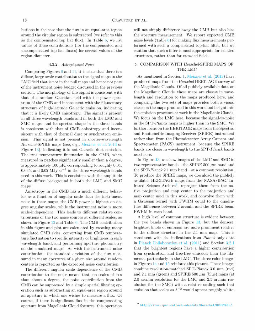
18 Crawford et al.

butions in the case that the flux in an equal-area region

around the circular region is subtracted (we refer to this

as the compensated top hat flux). In Table 6, we list

values of these contributions (for the compensated and

uncompensated top hat fluxes) for several values of the

region diameter.

4.3.2. Astrophysical Noise

Comparing Figures 6 and 11, it is clear that there is a

diffuse, large-scale contribution to the signal maps in the

LMC field that is not in the null maps and hence not part

of the instrument noise budget discussed in the previous

section. The morphology of this signal is consistent with

that of a random Gaussian field with the power spec-

trum of the CMB and inconsistent with the filamentary

structure of high-latitude Galactic emission, indicating

that it is likely CMB anisotropy. The signal is present

in all three wavelength bands and in both the LMC and

SMC maps, and its spectral shape in the three bands

is consistent with that of CMB anisotropy and incon-

sistent with that of thermal dust or synchrotron emis-

sion. This signal is not present in shorter-wavelength

Herschel-SPIRE maps (see, e.g., Meixner et al. 2013 or

Figure 13), indicating it is not Galactic dust emission.

The rms temperature fluctuation in the CMB, when

measured in patches significantly smaller than a degree,

is approximately 100 µK, corresponding to roughly 0.04,

0.035, and 0.02 MJy sr−1 in the three wavelength bands

used in this work. This is consistent with the amplitude

of the diffuse background in both the LMC and SMC

maps.

Anisotropy in the CMB has a much different behav-

ior as a function of angular scale than the instrument

noise in these maps: the CMB power is highest on de-

gree angular scales, while the instrument noise is more

scale-independent. This leads to different relative con-

tributions of the two noise sources at different scales, as

shown in Figure 12 and Table 6. The CMB contribution

in this figure and plot are calculated by creating many

simulated CMB skies, converting from CMB tempera-

ture fluctuation to specific intensity or brightness in each

wavelength band, and performing aperture photometry

on the simulated maps. As with the instrument noise

contribution, the standard deviation of the flux mea-

sured in many apertures of a given size around random

centers is reported as the expected noise contribution.

The different angular scale dependence of the CMB

contribution to the noise means that, on scales of less

than about a degree, the noise contribution from the

CMB can be suppressed by a simple spatial filtering op-

eration such as subtracting an equal-area region around

an aperture in which one wishes to measure a flux. Of

course, if there is significant flux in the compensating

aperture from Magellanic Cloud features, this operation

will not simply difference away the CMB but also bias

the aperture measurement. We report expected CMB

noise levels (Table 6) for making flux measurements per-

formed with such a compensated top-hat filter, but we

caution that such a filter is most appropriate for isolated

structures, rather than for crowded fields.

5. COMPARISON WITH Herschel-SPIRE MAPS OF

THE LMC

As mentioned in Section 1, Meixner et al. (2013) have

produced maps from the Herschel HERITAGE survey of

the Magellanic Clouds. Of all publicly available data on

the Magellanic Clouds, these maps are closest in wave-

length and resolution to the maps produced here, and

comparing the two sets of maps provides both a visual

check on the maps produced in this work and insight into

the emission processes at work in the Magellanic Clouds.

We focus on the LMC here, because the signal-to-noise

in the SPT-Planck maps is higher than in the SMC. We

further focus on the HERITAGE maps from the Spectral

and Photometric Imaging Receiver (SPIRE) instrument

rather than from the Photodetector Array Camera and

Spectrometer (PACS) instrument, because the SPIRE

bands are closer in wavelength to the SPT-Planck bands

used here.

In Figure 13, we show images of the LMC and SMC in

two representative bands—the SPIRE 500 µm band and

the SPT-Planck 2.1 mm band—at a common resolution.

To produce the SPIRE maps, we download the publicly

available HERITAGE maps from the NASA/IPAC In-

frared Science Archive7, reproject them from the na-

tive projection and map center to the projection and

map center used in this work, and convolve them with

a Gaussian kernel with FWHM equal to the quadra-

ture difference between 2 arcmin and the SPIRE beam

FWHM in each band.

A high level of common structure is evident between

the two bands shown in Figure 13, but the densest,

brightest knots of emission are more prominent relative

to the diffuse structure in the 2.1 mm map. This is

consistent with the indications from Planck-only data

in Planck Collaboration et al. (2011) and Section 3.2.1

that the brightest regions have a higher contribution

from synchrotron and free-free emission than the fila-

ments, particularly in the LMC. The three-color images

in Figures 14 and 15 reinforce this picture. These images

combine resolution-matched SPT-Planck 3.0 mm (red)

and 2.1 mm (green) and SPIRE 500 µm (blue) maps (at

2.0 arcmin resolution for the LMC and 2.5 arcmin res-

olution for the SMC) with a relative scaling such that

emission that scales as λ−2 would appear roughly white.

7 http://irsa.ipac.caltech.edu/data/Herschel/HERITAGE/

SPT-Planck maps of the Magellanic Clouds 19

(a) LMC null map, 1.4 mm (b) LMC null map, 2.1 mm (c) LMC null map, 3.0 mm

Figure 11. Combined SPT-Planck null maps of the 7.5-by-7.5-degree LMC field in three wavelength bands. Null maps arecreated by subtracting one half of the data from the other half and dividing by two. The 1.4 mm and 2.1 mm are at 1.5-arcminresolution; the 3.0 mm map is at 2.0-arcmin resolution. The units of the maps are MJy sr−1. The localized feature at roughly[85,−69] in the 3.0 mm map is a residual of the bright LMC source 30 Doradus (see Sections 2.1.2 and 2.2 for details). Forall images, we have used the combined null maps constructed assuming an emission spectrum I(λ) ∝ λ−2.

(a) Uncompensated aperture (b) Compensated aperture

Figure 12. Expected contributions from instrument noise and CMB anisotropy to the uncertainty on a measurement of fluxin the LMC field within an aperture as a function of aperture size. The instrument noise values in both panels are estimatedfrom the SPT+Planck null maps at 2.0-arcmin resolution, and the CMB values are estimated from simulated CMB maps with2.0-arcmin resolution. The behavior at 1.5 and 2.5-arcmin resolution is qualitatively similar except at the smallest aperture,and the behavior in the SMC field is nearly identical, but with slightly higher instrument noise values. Values at particularaperture sizes for all map resolutions and both fields are shown in Table 6. Values shown in the left panel are calculated withno compensating negative region around the aperture; values shown in the right panel are calculated with the flux from anequal-area region surrounding the aperture subtracted. For apertures smaller than ∼ 30 arcmin, this compensation significantlyreduces the contribution from the CMB at the expense of increasing the instrument noise contribution (by roughly a factor of√

2).

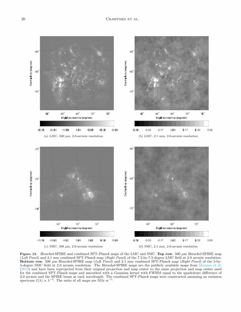
20 Crawford et al.

(a) LMC, 500 µm, 2.0-arcmin resolution (b) LMC, 2.1 mm, 2.0-arcmin resolution

(c) SMC, 500 µm, 2.0-arcmin resolution (d) SMC, 2.1 mm, 2.0-arcmin resolution

Figure 13. Herschel-SPIRE and combined SPT-Planck maps of the LMC and SMC. Top row: 500 µm Herschel-SPIRE map(Left Panel) and 2.1 mm combined SPT-Planck map (Right Panel) of the 7.5-by-7.5-degree LMC field at 2.0 arcmin resolution.Bottom row: 500 µm Herschel-SPIRE map (Left Panel) and 2.1 mm combined SPT-Planck map (Right Panel) of the 5-by-5-degree SMC field at 2.0 arcmin resolution. The Herschel-SPIRE maps are the publicly available maps from Meixner et al.(2013) and have been reprojected from their original projection and map center to the same projection and map center usedfor the combined SPT-Planck maps and smoothed with a Gaussian kernel with FWHM equal to the quadrature difference of2.0 arcmin and the SPIRE beam at each wavelength. The combined SPT-Planck maps were constructed assuming an emissionspectrum I(λ) ∝ λ−2. The units of all maps are MJy sr−1.

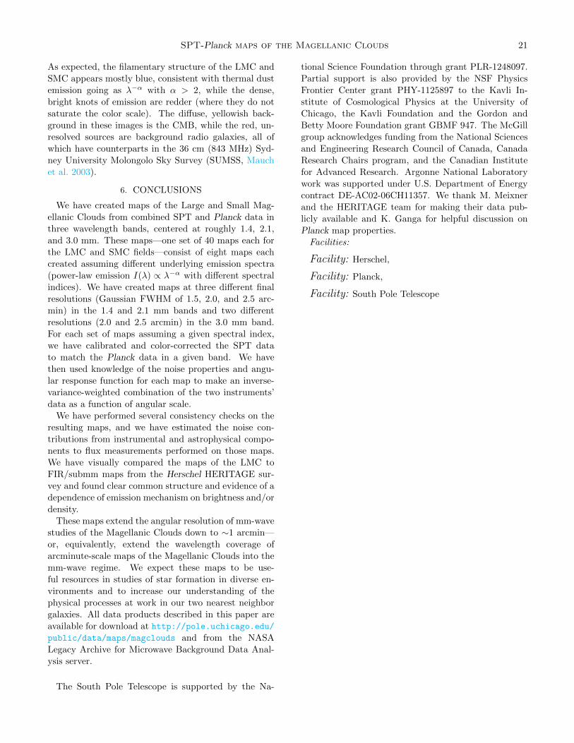
SPT-Planck maps of the Magellanic Clouds 21

As expected, the filamentary structure of the LMC and

SMC appears mostly blue, consistent with thermal dust

emission going as λ−α with α > 2, while the dense,

bright knots of emission are redder (where they do not

saturate the color scale). The diffuse, yellowish back-

ground in these images is the CMB, while the red, un-

resolved sources are background radio galaxies, all of

which have counterparts in the 36 cm (843 MHz) Syd-

ney University Molongolo Sky Survey (SUMSS, Mauch

et al. 2003).

6. CONCLUSIONS

We have created maps of the Large and Small Mag-

ellanic Clouds from combined SPT and Planck data in

three wavelength bands, centered at roughly 1.4, 2.1,

and 3.0 mm. These maps—one set of 40 maps each for

the LMC and SMC fields—consist of eight maps each

created assuming different underlying emission spectra

(power-law emission I(λ) ∝ λ−α with different spectral

indices). We have created maps at three different final

resolutions (Gaussian FWHM of 1.5, 2.0, and 2.5 arc-

min) in the 1.4 and 2.1 mm bands and two different

resolutions (2.0 and 2.5 arcmin) in the 3.0 mm band.

For each set of maps assuming a given spectral index,

we have calibrated and color-corrected the SPT data

to match the Planck data in a given band. We have

then used knowledge of the noise properties and angu-

lar response function for each map to make an inverse-

variance-weighted combination of the two instruments’

data as a function of angular scale.

We have performed several consistency checks on the

resulting maps, and we have estimated the noise con-

tributions from instrumental and astrophysical compo-

nents to flux measurements performed on those maps.

We have visually compared the maps of the LMC to

FIR/submm maps from the Herschel HERITAGE sur-

vey and found clear common structure and evidence of a

dependence of emission mechanism on brightness and/or

density.

These maps extend the angular resolution of mm-wave

studies of the Magellanic Clouds down to ∼1 arcmin—

or, equivalently, extend the wavelength coverage of

arcminute-scale maps of the Magellanic Clouds into the

mm-wave regime. We expect these maps to be use-

ful resources in studies of star formation in diverse en-

vironments and to increase our understanding of the

physical processes at work in our two nearest neighbor

galaxies. All data products described in this paper are

available for download at http://pole.uchicago.edu/

public/data/maps/magclouds and from the NASA

Legacy Archive for Microwave Background Data Anal-

ysis server.

The South Pole Telescope is supported by the Na-

tional Science Foundation through grant PLR-1248097.

Partial support is also provided by the NSF Physics

Frontier Center grant PHY-1125897 to the Kavli In-

stitute of Cosmological Physics at the University of

Chicago, the Kavli Foundation and the Gordon and

Betty Moore Foundation grant GBMF 947. The McGill

group acknowledges funding from the National Sciences

and Engineering Research Council of Canada, Canada

Research Chairs program, and the Canadian Institute

for Advanced Research. Argonne National Laboratory

work was supported under U.S. Department of Energy

contract DE-AC02-06CH11357. We thank M. Meixner

and the HERITAGE team for making their data pub-

licly available and K. Ganga for helpful discussion on

Planck map properties.

Facilities:

Facility: Herschel,

Facility: Planck,

Facility: South Pole Telescope

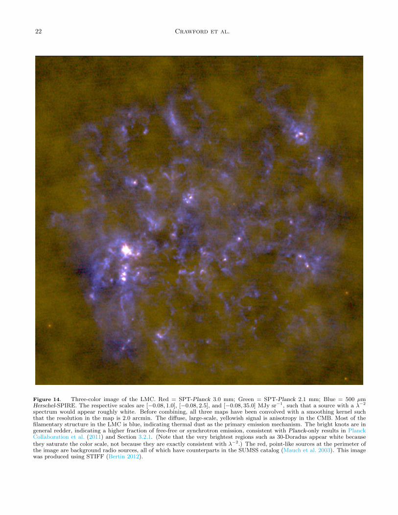
22 Crawford et al.

Figure 14. Three-color image of the LMC. Red = SPT-Planck 3.0 mm; Green = SPT-Planck 2.1 mm; Blue = 500 µmHerschel-SPIRE. The respective scales are [−0.08, 1.0], [−0.08, 2.5], and [−0.08, 35.0] MJy sr−1, such that a source with a λ−2

spectrum would appear roughly white. Before combining, all three maps have been convolved with a smoothing kernel suchthat the resolution in the map is 2.0 arcmin. The diffuse, large-scale, yellowish signal is anisotropy in the CMB. Most of thefilamentary structure in the LMC is blue, indicating thermal dust as the primary emission mechanism. The bright knots are ingeneral redder, indicating a higher fraction of free-free or synchrotron emission, consistent with Planck-only results in PlanckCollaboration et al. (2011) and Section 3.2.1. (Note that the very brightest regions such as 30-Doradus appear white becausethey saturate the color scale, not because they are exactly consistent with λ−2.) The red, point-like sources at the perimeter ofthe image are background radio sources, all of which have counterparts in the SUMSS catalog (Mauch et al. 2003). This imagewas produced using STIFF (Bertin 2012).

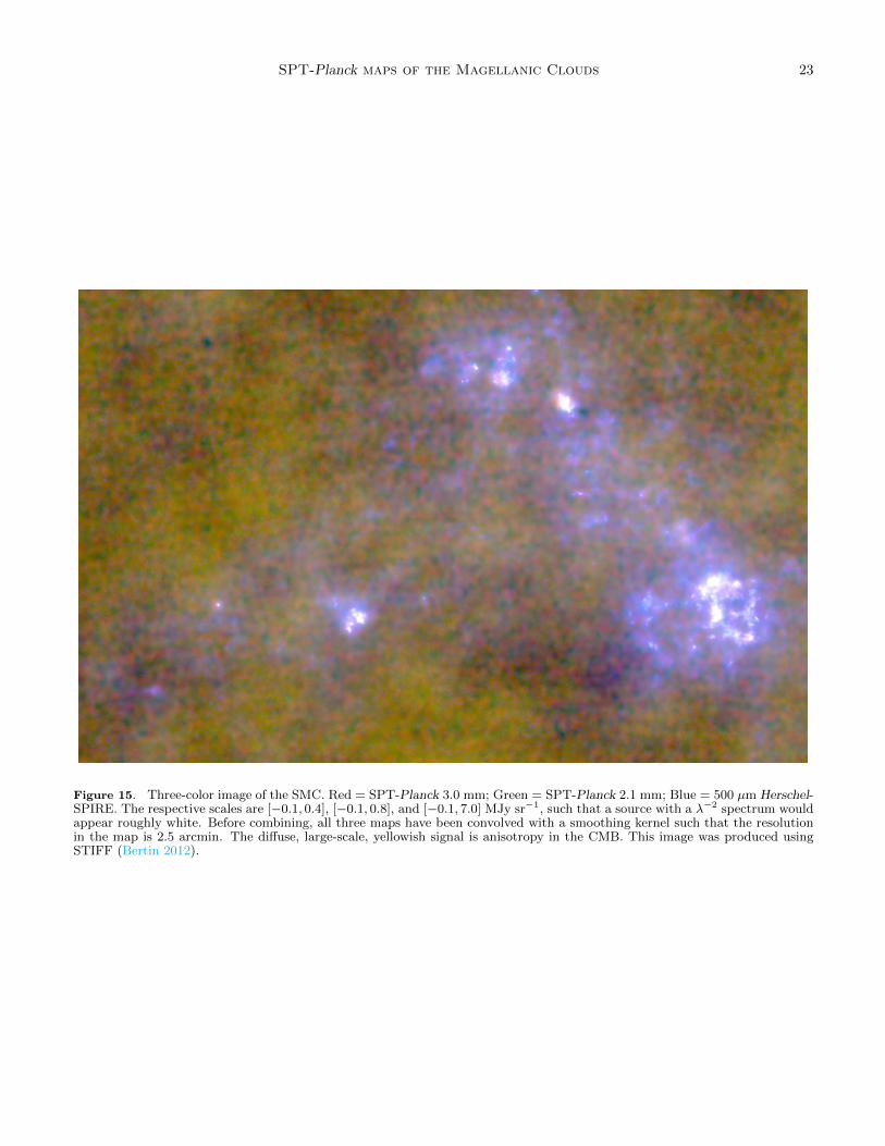
SPT-Planck maps of the Magellanic Clouds 23

Figure 15. Three-color image of the SMC. Red = SPT-Planck 3.0 mm; Green = SPT-Planck 2.1 mm; Blue = 500 µm Herschel-SPIRE. The respective scales are [−0.1, 0.4], [−0.1, 0.8], and [−0.1, 7.0] MJy sr−1, such that a source with a λ−2 spectrum wouldappear roughly white. Before combining, all three maps have been convolved with a smoothing kernel such that the resolutionin the map is 2.5 arcmin. The diffuse, large-scale, yellowish signal is anisotropy in the CMB. This image was produced usingSTIFF (Bertin 2012).

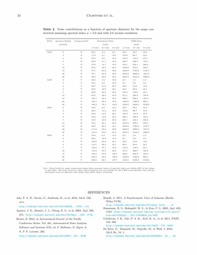
24 Crawford et al.

Table 2. Noise contributions as a function of aperture diameter for the maps con-

structed assuming spectral index α = 2.0 and with 2.0 arcmin resolution.

Field Aperture Radius Compensated? Instrument Noise CMB Noise

[arcmin] [mJy] [mJy]

1.4 mm 2.1 mm 3.2 mm 1.4 mm 2.1 mm 3.2 mm

LMC 2 N 20.5 5.4 9.6 46.9 38.7 24.3

3 N 17.8 8.1 12.5 104.9 86.7 54.4

4 N 27.9 9.6 14.9 187.3 154.8 97.2

5 N 28.8 11.1 16.3 289.1 238.9 150.1

7 N 37.9 14.1 19.0 547.1 452.1 284.0

10 N 46.8 18.4 24.4 1055.9 872.5 548.1

15 N 57.7 27.6 30.9 2160.9 1785.6 1121.7

20 N 75.1 34.4 40.6 3500.9 2893.0 1817.3

30 N 99.4 52.3 53.5 6547.0 5410.0 3398.4

LMC 2 Y 38.2 5.2 10.8 2.3 1.9 1.2

3 Y 45.5 9.9 19.0 9.5 7.8 4.9

4 Y 68.7 15.3 25.7 23.9 19.8 12.4

5 Y 83.8 18.3 32.1 48.3 39.9 25.1

7 Y 99.6 23.4 44.9 125.3 103.6 65.1

10 Y 82.5 32.9 57.6 317.1 262.0 164.6

15 Y 116.1 44.4 73.9 838.5 692.9 435.3

20 Y 156.7 50.1 77.6 1656.9 1369.2 860.1

30 Y 189.3 70.1 105.1 4158.5 3436.3 2158.6

SMC 2 N 32.9 8.0 15.2 46.9 38.7 24.3

3 N 28.9 11.3 18.9 104.9 86.7 54.4

4 N 46.8 12.0 22.1 187.3 154.8 97.2

5 N 44.8 12.6 24.5 289.1 238.9 150.1

7 N 59.0 16.0 27.2 547.1 452.1 284.0

10 N 70.6 20.1 36.2 1055.9 872.5 548.1

15 N 92.9 26.5 44.1 2160.9 1785.6 1121.7

20 N 111.8 33.4 50.8 3500.9 2893.0 1817.3

30 N 144.5 53.0 68.4 6547.0 5410.0 3398.4

SMC 2 Y 56.8 8.4 17.5 2.3 1.9 1.2

3 Y 68.2 16.9 31.2 9.5 7.8 4.9

4 Y 104.6 23.6 45.1 23.9 19.8 12.4

5 Y 112.1 26.5 53.1 48.3 39.9 25.1

7 Y 133.0 37.1 70.2 125.3 103.6 65.1

10 Y 113.4 47.4 84.2 317.1 262.0 164.6

15 Y 176.9 57.0 100.1 838.5 692.9 435.3

20 Y 214.9 59.5 108.0 1656.9 1369.2 860.1

30 Y 290.2 86.5 137.7 4158.5 3436.3 2158.6

Note—Noise levels for maps constructed using other assumed values of spectral index are within 20% of the valuesin this table. The noise levels for other map resolutions are very similar for the CMB in all aperture sizes and forinstrument noise at aperture sizes larger than either map’s resolution.

REFERENCES

Ade, P. A. R., Savini, G., Sudiwala, R., et al. 2010, A&A, 520,

A11.

http://adsabs.harvard.edu/abs/2010A%26A...520A..11A

Aguirre, J. E., Bezaire, J. J., Cheng, E. S., et al. 2003, ApJ, 596,

273. http://adsabs.harvard.edu/abs/2003ApJ...596..273A

Bertin, E. 2012, in Astronomical Society of the Pacific

Conference Series, Vol. 461, Astronomical Data Analysis

Software and Systems XXI, ed. P. Ballester, D. Egret, &

N. P. F. Lorente, 263.

http://adsabs.harvard.edu/abs/2012ASPC..461..263B

Boselli, A. 2011, A Panchromatic View of Galaxies (Berlin:

Wiley-VCH).

http://adsabs.harvard.edu/abs/2011pvg..book.....B

Bussmann, R. S., Holzapfel, W. L., & Kuo, C. L. 2005, ApJ, 622,

1343. http://adsabs.harvard.edu/cgi-bin/nph-bib_query?

bibcode=2005ApJ...622.1343B&db_key=AST

Carlstrom, J. E., Ade, P. A. R., Aird, K. A., et al. 2011, PASP,

123, 568.

http://adsabs.harvard.edu/abs/2011PASP..123..568C

De Zotti, G., Massardi, M., Negrello, M., & Wall, J. 2010,

A&A Rv, 18, 1.

http://adsabs.harvard.edu/abs/2010A%26ARv..18....1D

SPT-Planck maps of the Magellanic Clouds 25

George, E. M., Reichardt, C. L., Aird, K. A., et al. 2015, ApJ,

799, 177.http://adsabs.harvard.edu/abs/2015ApJ...799..177G

Healey, S. E., Romani, R. W., Taylor, G. B., et al. 2007, ApJS,

171, 61.http://adsabs.harvard.edu/abs/2007ApJS..171...61H

Israel, F. P., Wall, W. F., Raban, D., et al. 2010, A&A, 519, A67.http://adsabs.harvard.edu/abs/2010A%26A...519A..67I

Lamarre, J.-M., Puget, J.-L., Ade, P. A. R., et al. 2010, A&A,

520, A9.http://adsabs.harvard.edu/abs/2010A%26A...520A...9L

Mauch, T., Murphy, T., Buttery, H. J., et al. 2003, MNRAS,

342, 1117. http://adsabs.harvard.edu/cgi-bin/bib_query?

2003MNRAS.342.1117M

Meixner, M., Panuzzo, P., Roman-Duval, J., et al. 2013, AJ, 146,

62. http://adsabs.harvard.edu/abs/2013AJ....146...62M

Mizuno, N. 2009, in IAU Symposium, Vol. 256, The Magellanic

System: Stars, Gas, and Galaxies, ed. J. T. Van Loon & J. M.

Oliveira, 203–214.http://adsabs.harvard.edu/abs/2009IAUS..256..203M

Murphy, T., Sadler, E. M., Ekers, R. D., et al. 2010, MNRAS,402, 2403.

http://adsabs.harvard.edu/abs/2010MNRAS.402.2403M

Ott, J., Wong, T., Pineda, J. L., et al. 2008, PASA, 25, 129.http://adsabs.harvard.edu/abs/2008PASA...25..129O

Padin, S., Staniszewski, Z., Keisler, R., et al. 2008, ApOpt, 47,

4418. http://adsabs.harvard.edu/abs/2008ApOpt..47.4418P

Planck Collaboration, Ade, P. A. R., Aghanim, N., et al. 2011,

A&A, 536, A17.

http://adsabs.harvard.edu/abs/2011A%26A...536A..17P

—. 2014a, A&A, 571, A1.

http://adsabs.harvard.edu/abs/2014A%26A...571A...1P

—. 2014b, A&A, 571, A8.

http://adsabs.harvard.edu/abs/2014A%26A...571A...8P

—. 2014c, A&A, 571, A6.

http://adsabs.harvard.edu/abs/2014A%26A...571A...6P

—. 2014d, A&A, 571, A9.

http://adsabs.harvard.edu/abs/2014A%26A...571A...9P

Planck Collaboration, Ade, P. A. R., Alves, M. I. R., et al. 2015,

A&A, 576, A107.

http://adsabs.harvard.edu/abs/2015A%26A...576A.107P

Planck Collaboration, Adam, R., Ade, P. A. R., et al. 2016a,

A&A, 594, A8.

http://adsabs.harvard.edu/abs/2016A%26A...594A...8P

—. 2016b, A&A, 594, A1.

http://adsabs.harvard.edu/abs/2016A%26A...594A...1P

Planck HFI Core Team, Ade, P. A. R., Aghanim, N., et al. 2011,

A&A, 536, A6.

http://adsabs.harvard.edu/abs/2011A%26A...536A...6P

Schaffer, K. K., Crawford, T. M., Aird, K. A., et al. 2011, ApJ,

743, 90.

http://adsabs.harvard.edu/abs/2011ApJ...743...90S

Westerlund, B. E. 1997, The Magellanic Clouds (Ca: Cambridge

University Press).

http://adsabs.harvard.edu/abs/1997macl.book.....W