Embed Size (px)
Citation preview

1
Exam 2 AERE331 Spring 2020 Take-Home Exam 2 Due 3/27(F) SOLUTION
PROBLEM 1(20pts) This problem addresses the recovery of a model transfer function from an experimentally obtained
Bode plot.
(a)(15pts) Use straight-line approximations to recover a model transfer function from the Bode plot at right. Use both
magnitude and phase straight-line approximations. {Note; Use a ruler to draw lines, and estimate slopes.]
Figure 1(a) Experimentally obtained Bode plot.
Solution:
(i): Clearly, there is a second order underdamped component with 20n [ 90o ]and
15/2015 10 1/ 2 0.09Q dB . Hence: 1 11 2 2 2( )
2 3.6 400n n
c cG s
s s s s
.
(ii): There is a second first order term [ 60 / ]dB dec with 1 1000 [ 225o ]. Hence: 2
2 ( )1000
cG s
s
.
(iii): 1 21 2 2
( ) ( ) ( )( 3.6 400)( 1000)
c cG s G s G s
s s s
has 1 2(0)
400(1000)s
c cg G . From the plot we have
30/2030 10dBs sg dB g 0.0316 . This gives 1 2
1 250.0316 5440
4(10 )
c cc c . So:
2
5440( )
( 3.6 400)( 1000)G s
s s s
.
(b)(5pts) Give a Bode plot of your model. Then comment.
Solution: [See code @ 1(b).]
Visually, it appears to be quite similar to Figure 1(a).
Figure 1(b) Model Bode plot
60 100 40 /dB dec
150 210 60 /dB dec
( 180 270) / 2 45 /o dec
0 90 90 /o dec
~15dB
n

2
PROBLEM 2(45pts) Consider the feedback system at right that is used
to control the angular position of a robotic manipulator arm.
(a)(10pt) Use a Bode plot to design a controller ( )a
cG K to satisfy the
single specification (S1) 70oPM . Verify your design using the
command: [GM PM wpc wgc]=margin(Ga).
Solution: [See code @ 2(a).]
23.2/2023.2 10 0.0692dBK K . So: ( ) 0.0692a
cG .
[GM PM wpc wgc]=margin(Ga)
GM = 2.0552 PM = 69.9440 wpc = 2.5820 wgc = 0.9354
Figure 2(a) Bode plot.
(b)(10pts) For the additional specification (S2) 3 /gc r s design a
non-unity double-lead compensator. Verify your design using the
margin command.
Solution: [See code @ 2(b).]
We need to add 96o at max 1 2 3 /r s . This will require a
double-lead compensator with each component giving 48o.
2
1
1 sin(48 )6.7825 ( 16.633 )
1 sin(48 )
o
odB
. Hence,
1 max / 1.1516 and 2 1 7.8153 . The double-lead
compensator will add 16.663dB to the already 14.3dB giving
30.963dB. Hence, we need 30.963/2010 0.0283K .
The compensator is then:
2 2 2
( ) 7.8153 1.1516 1.1516.0283 1.3034
1.1516 7.8153 7.8153
b
c
s sG
s s
. Figure2(b) Bode plot.
[GM PM wpc wgc]=margin(Gb) GM =2.9525 PM = 68.5527 wpc = 5.1422 wgc =3.0223
ref 2
20
2 8s s ( )cG s
armmotorcontroller
50
( 10)s s

3
(c)(10pts) (i) Overlay the CL Bode plots and use the data cursor to obtain the -3dB BW for each system. (ii) Overlay the
OL Bode plots and use the data cursor to identify all gain crossover frequencies. (iii) Explain why, in view of (ii), you
think that even though the design in (b) specified a value for gc that was three times that in (a), the CL BW for (b) is
significantly less than that for (a).
Solution: [See code @ 2(c).]
Figure 3(c1) CL Bode plots with data cursor information.
(i): The -3dB BW of Wa is 2.8 rad/s and for Wb it is 0.28 rad/sec.
Figure 3(c2) OL Bode plots and data cursor information.
(ii) Ga has one crossover frequency at 0.938 rad/sec and Gb has one at 0.402 rad/sec and a second at 3.02 rad/sec.
(iii) The reason is that Gb has two crossover frequencies, including a very low one .
4
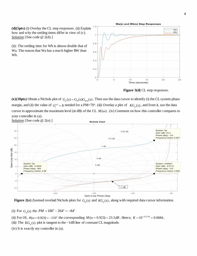
(d)(5pts) (i) Overlay the CL step responses. (ii) Explain
how and why the settling times differ in view of (c).
Solution: [See code @ 2(d).]
(ii): The settling time for Wb is almost double that of
Wa. The reason that Wa has a much higher BW than
Wb.
Figure 3(d) CL step responses.
(e)(10pts) Obtain a Nichols plot of ( ) ( ) ( )p m armG s G s G s . Then use the data cursor to identify (i) the CL system phase
margin, and (ii) the value of ( )a
cG K needed for a PM=70o. (iii) Overlay a plot of ( )pKG s , and from it, use the data
cursor to approximate the maximum level (in dB) of the CL ( )M . (iv) Comment on how this controller compares to
your controller in (a).
Solution: [See code @ 2(e).]
Figure 2(e) Zoomed overlaid Nichols plots for ( )pG s and ( )pKG s , along with required data cursor information.
(i): For ( )pG s the 180 264 84o o oPM
(ii) For OL ( 0.923) 110o the corresponding ( 0.923) 23.3M dB . Hence, 23.3/2010 0.0684K .
(iii) The ( )pKG s plot is tangent to the ~1dB line of constant CL magnitude.
(iv) It is exactly my controller in (a).

5
PROBLEM 3(35pts) The plant TF for attitude is [see Nelson p.295]: 2
20( 10) ( )( )
0.65 2.15 ( )p
e
s sG s
s s s
.
(a)(10pts) (i) Develop the controller canonical state space representation for ( )pG s . (ii) Verify your answer by using the
ss2tf command.
Solution: [Give your code/results HERE.]
(i): 2 ( ) 0.65 ( ) 2.15 ( ) ( )es V s sV s V s s gives 0.65 2.15 ev v v . Let 1 2;x v x v .
Then 1 2( ) (20 200) ( ) 20 200 20 200s s V s v v x x . Hence, we arrive at:
0.65 2.15 1
1 0 0e
x x and 20 200 0 e x .
(ii): A=[-0.65 -2.15 ; 1 0]; B=[1;0]; C=[20 200]; D=0;
[np,dp]=ss2tf(A,B,C,D) np =[ 0 20 200 ] dp = [1.00 0.65 2.15 ]. Verified.
(b)(10pts) (i) Obtain the state controller that will achieve closed loop poles having 0.25 and 0.9 . (ii) Use the CL
A-matrix to verify your design. Show ALL work.
Solution: [Give code/results HERE.]
(i): 0.25 4 4.4444 4.4444 1 .81 1.9373n n d . Hence, 1,2 4 1.9373s i .
s1=-4+1i*1.9373; s2=conj(s1); K=place(A,B,[s1 s2]) = [ 7.3500 17.6031 ]
(ii): ACL=A-B*K; eigs(ACL) = -4.0000 +/- 1.9373i
(c)(10pts) To arrive at a CL transfer function having unity static
gain: (i)Use the ss2tf command to obtain the regulator TF. Then
(ii) scale it to have unity static gain. Give the CL tF and plot the
unit step response.
Solution: [Give code/results HERE.]
[n0 d0]=ss2tf(ACL,B,C,D) n0 =[0 20 200] ; d0 = [1 8 19.7531]
sf=d0(3)/n0(3); W=tf(sf*n0,d0)
W = (1.975 s + 19.75)/(s^2 + 8 s + 19.75)
Figure 3(c) CL command system step response.
(d)(5pts) (i) Develop a PD controller in the usual (not state space) manner. (ii) Obtain the CL TF. (iii) overlay the step
response on the plot in (c). (iv) The initial behavior in your plot should be strangese the initial value theorem to explain
why.
Solution: 21 21 22
(20 200)( )( ) ( ) ( 0.65 2.15) (20 200)( )
0.65 2.15
s K s KG s p s s s s K s K
s s
2
1 1 2 2( ) (1 20 ) (0.65 200 20 ) (2.15 200 )p s K s K K s K
2 21 2 2
1 1
0.65 200 20 2.15 200( ) 8 19.75
1 20 1 20
K K Kp s s s s s
K K
. This gives 1 2 .0703 .2269K K (using a matrix eqn.)
(ii): The CL TF is: Wd = (1.406 s^2 + 18.6 s + 45.38)/(2.406 s^2 + 19.25 s + 47.53)
(iii) For a unit step input, the initial value theorem gives:
0lim ( ) lim ( ) lim ( )(1/ ) lim ( ) 1.406 / 2.406 0.5844t s s s
t s s sW s s W s
. This is shown in the figure. Even though W(s) is a
proper TF, it is not strictly proper. What we see here is that the initial angular velocity is infinite.

6
Appendix Matlab Code %PROGRAM NAME: exam2.m (3/13/20)
%PROBLEM 1
%TRUE TF:
s=tf('s');
G=10000/((s^2+4*s+400)*(s+1000));
title('Experimentally Obtained Bode Plot')
grid
%(b):
s=tf('s');
Ghat=5440/((s^2+3.6*s+400)*(s+1000));
figure(10)
bode(Ghat)
grid
%=========================================
%PROBLEM 2
%(a):
Garm=20/(s^2+2*s+8); Gm=50/(s*(s+10));
Gp=Gm*Garm;
figure(20)
bode(Gp)
grid
K=0.0692;
Ga=K*Gp;
[GM PM wpc wgc]=margin(Ga)
%------------
%(b):
figure(21)
bode(Gp)
grid
Gcb=1.3034*(s+1.1516)^2/(s+7.8153)^2;
Gb=Gcb*Gp;
[GM PM wpc wgc]=margin(Gb)
%------------
%(c):
Wa=feedback(Ga,1);
Wb=feedback(Gb,1);
figure(22)
bode(Wa,Wb)
title('Wa(s) and Wb(s)Bode Plots')
grid
legend('Wa','Wb')
figure(23)
bode(Ga,Gb)
title('Ga(s) and Gb(s)Bode Plots')
grid
legend('Ga','Gb')
%(d):
figure(23)
step(Wa,Wb)
title('Wa(s) and Wb(s) Step Responses')
grid
legend('Wa','Wb')
%(e):
figure(24)
nichols(Gp)
grid
KdB=-23.3; K=10^(KdB/20)
hold on
nichols(K*Gp)
%===================================================
%PROBLEM 3
%(a):
A=[-0.65 -2.15 ; 1 0];
B=[1;0]; C=[20 200]; D=0;
[np,dp]=ss2tf(A,B,C,D)
%(b):
s1=-4+1i*1.9373; s2=conj(s1);
K=place(A,B,[s1 s2])
ACL=A-B*K;
eigs(ACL);
%(c):
[n0 d0]=ss2tf(ACL,B,C,D)

7
sf=d0(3)/n0(3);
W=tf(sf*n0,d0)
figure(30)
step(W)
grid
%(d):
Gp=(20*s+200)/(s^2+.65*s+2.15);
Gcd=.0703*s+.2269;
Wd=feedback(Gcd*Gp,1)
hold on
step(Wd)
legend('W','Wd')