Embed Size (px)
Citation preview

Please cite this paper as:
Jacobzone, S. et al. (2010), “Assessing the Impact ofRegulatory Management Systems: Preliminary Statisticaland Econometric Estimates”, OECD Working Papers onPublic Governance, No. 17, OECD Publishing.doi: 10.1787/5kmfq1pch36h-en
OECD Working Papers on PublicGovernance No. 17
Assessing the Impact ofRegulatory ManagementSystems
PRELIMINARY STATISTICAL ANDECONOMETRIC ESTIMATES
Stéphane Jacobzone*, Faye Steiner,Erika L. Ponton, Emmanuel Job
*OECD, France


OECD WORKING PAPERS ON PUBLIC GOVERNANCE
No. 17
ASSESSING THE IMPACT OF REGULATORY MANAGEMENT SYSTEMS: PRELIMINARY STATISTICAL
AND ECONOMETRIC ESTIMATES
Stéphane Jacobzone, Regulatory Policy Division, OECD
Faye Steiner, Stanford University, University of Paris I
Erika Lopez Ponton, University of Paris I
Emmanuel Job, Regulatory Policy Division, OECD

2
The OECD is a unique forum where the governments of 31 democracies work together to address
the economic, social and environmental challenges of globalisation. The OECD is also at the forefront of
efforts to understand and to help governments respond to new developments and concerns, such as
corporate governance, the information economy and the challenges of an ageing population. The
Organisation provides a setting where governments can compare policy experiences, seek answers to
common problems, identify good practice and work to co-ordinate domestic and international policies.
The OECD member countries are: Australia, Austria, Belgium, Canada, Chile, the Czech Republic,
Denmark, Finland, France, Germany, Greece, Hungary, Iceland, Ireland, Italy, Japan, Korea,
Luxembourg, Mexico, the Netherlands, New Zealand, Norway, Poland, Portugal, the Slovak Republic,
Spain, Sweden, Switzerland, Turkey, the United Kingdom and the United States. The Commission of the
European Communities takes part in the work of the OECD.
This project received significant financial assistance of the European Commission, which
made it possible to perform a full analysis of the data. The views expressed herein can in
no way be taken to reflect the official opinion of the European Commission.
© OECD 2010.
3
ABSTRACT
Assessing the impact of regulatory management systems:
Preliminary statistical and econometric estimates This Working Paper presents preliminary analytical estimates using the 1998 and 2005 surveys of
indicators of systems for the management of regulatory quality. Two broad dimensions are found in
regulatory management systems using Factor Analysis, and Principal Component Analysis. The first
reflects an integrated approach to ex ante assessment, with the use of tools such as formal consultation and
regulatory impact analysis as well as institutions for regulatory oversight, training and capacity building.
The second focuses on the stock of regulation, with administrative simplification, streamlining licences and
permits, etc. These data are correlated with other available datasets on regulatory frameworks, including
the OECD indicators of Product Market Regulations, subsets of the Doing business and Worldwide
Governance Indicators (WGI) from the World Bank and the Global Competitiveness Index (GCI) from the
World Economic Forum. Finally, the report presents some preliminary regressions with reduced forms,
including fixed and random effects, linking the indicators to macroeconomic indicators. The findings tend
to support the view that improvements in regulatory management system quality yield significant
economic benefits.
Note: Stephane Jacobzone is a senior economist, and Emmanuel Job, statistician in the Regulatory
Policy Division at the OECD. The econometric analysis was prepared by Prof Faye Steiner, Economics
Department, Stanford University and Erika Lopez Ponton, University of Paris I Sorbonne, Economics
Department, at the time the report was drafted. Stephane Jacobzone would like to thank Sander Wagner for
his outstanding research assistance. The authors would like to thank the following OECD staffs for their
comments: in the OECD Public Governance and Territorial Development Directorate: Christiane Arndt,
Gregory Bounds and Josef Konvitz from the Regulatory Policy Division, Zsuzsanna Lonti and Laurent
Nahmias in the Public Sector Management and Performance Division. In the Economics Department: Paul
Conway, economist at the time the report was drafted. The authors would also like to thank the network of
national delegates and experts who provided feedback and inputs, as well as participants to the workshop
organised in London in March 2009. Any potential errors remain the authors’ responsibility.

4
TABLE OF CONTENTS
INTRODUCTION ........................................................................................................................................... 6
I. INDICATORS OF REGULATORY MANAGEMENT SYSTEMS: AN ANALYTICAL OVERVIEW .. 7
Mapping core dimensions of regulatory management systems quality through principal Component
Analysis ....................................................................................................................................................... 7 The Regulatory Management System Dataset ............................................................................................. 9
Analysis of the correlation between the variables .................................................................................. 12 The principal component approach ............................................................................................................ 13
Number of Principal Components retained ............................................................................................ 13 Regulatory Policy Management in 2005: two core dimensions ............................................................. 14
Typologies of country approaches to regulatory quality in 1998 and 2005 ............................................... 17
II. TESTING HOMOGENEITY AND CONSISTENTY OF REGULATORY
MANAGEMENT SYSTEM INDICATORS WITH EXTERNAL INDICES .............................................. 21
The indicators used for the correlations ..................................................................................................... 21 External indicators.................................................................................................................................. 21 OECD Product Market regulation indicator (PMR) and Regulatory Reform Index (REGREF) ........... 24 OECD Regulatory Management System Indicators ............................................................................... 25
Results from the correlations ..................................................................................................................... 25 Doing Business ....................................................................................................................................... 25 Global Competitiveness Index (GCI) ..................................................................................................... 26 Worldwide Governance Indicators (WGI) ............................................................................................. 26 OECD Product Market Regulation and REGREF Indicators................................................................. 27 Dynamic correlations with OECD Product Market Regulation and REGREF Indicators ..................... 28
III. ASSESSING THE IMPACT OF SYSTEMS FOR THE MANAGEMENT
OF REGULATORY QUALITY FOR ECONOMIC GROWTH .................................................................. 30
Overview .................................................................................................................................................... 30 The modelling strategy .............................................................................................................................. 30 Data ............................................................................................................................................................ 32
Dependent Variables .............................................................................................................................. 32 Exogenous variables of regulatory management quality........................................................................ 33
Results ........................................................................................................................................................ 33 Fixed effect regressions .......................................................................................................................... 33 Random effect regressions ..................................................................................................................... 34 Product Market Regulation Indicators ................................................................................................... 34 Summary ................................................................................................................................................ 35
IV. CONCLUSIONS ..................................................................................................................................... 36
BIBLIOGRAPHY ......................................................................................................................................... 38
ANNEX A1 ................................................................................................................................................... 40
Description of external indicators .............................................................................................................. 47 Doing Business Indicator (DBI) ............................................................................................................. 47 Global Competitiveness Index (GCI) ..................................................................................................... 48 The OECD Regulatory Management System indicator ......................................................................... 50
NOTE: FIXED VERSUS RANDOM EFFECTS .......................................................................................... 66

5
Tables
Table 1. List of policy areas of 2005 and 1998 surveys ...................................................................... 11 Table 2. Eigenvalue and share of total variance explained by the principal components ................... 13 Table 3. Component 1 – ...................................................................................................................... 15 Table 4. Component 2 – Stock Oriented Strategies, Simplification (SOSS), 2005 data ..................... 16 Table 5. Component 1 – The ............................................................................................................... 17 Table 6. Component 2 – Administrative simplification, due process 1998 data ................................. 17 Table 7. Doing Business indicators for the correlations (DB) ............................................................. 22 Table 8. Global Competitiveness Indicators for the correlations (GCI) .............................................. 23 Table 9. World Governance Indicators for the correlations (WGI) ..................................................... 23 Table 10. Global Competitiveness Indicators for the correlations (GCI) .............................................. 24 Table 11. OECD Indicators of Regulatory Management Systems ........................................................ 25 Table 12. Correlations of OECD RMS with World Bank Doing Business indicators .......................... 26 Table 13. Correlations of OECD RMS indicators with PMR and REGREF indicators 1998 ............... 27 Table 14. Correlations of OECD RMS indicators with PMR and REGREF Indicators 2005 ............... 28 Table 15. Correlations between changes in REGREF and Product
Market Regulation and administrative simplification policies .............................................. 29 Table A1.1. 2005 Data Correlation Matrix............................................................................................ 41 Table A1.2. 2005 Linked Data Correlation Matrix ............................................................................... 42 Table A1.3. 1998 Data Correlation Matrix............................................................................................ 43 Table A1.4. Principal components for 2005 data analysis .................................................................... 44 Table A1.5. Principal components for 2005 linked data analysis ......................................................... 45 Table A1.6. Principal components for 1998 data analysis .................................................................... 46 Table A1.7. Correlations of RMS with World Bank Doing Business Indicators .................................. 51 Table A1.8. Correlations of OECD RMS with WEF Global Competitiveness Indicators (2005) ........ 52 Table A1.9. Correlations of OECD RMS with World Bank Governance Indicators (2005) ................ 53 Table A1.10. Correlations of OECD RMS with World Bank Governance Indicators (1998) ............ 54 Table A1.11. Fixed effects regressions with RMS1 indicator ............................................................. 58 Table A1.12. Fixed effects regressions with RMS simple average indicator ...................................... 59 Table A1.13. Fixed Effects regressions with RMS weighted aggregated indicator ............................ 60 Table A1.14. Random Effects regressions with interpolated RMS 1 indicator ................................... 61 Table A1.15. Random effects regressions with interpolated RMS av indicator .................................. 62 Table A1.16 Random effects regressions with interpolated RMS ag indicator...................................... 63 Table A1.17. Fixed effects regressions with PMR indicator ............................................................... 64 Table A1.18. Random effects regressions with interpolated PMR indicator ...................................... 65
Figures
Figure 1. Policy areas covered by the 1998 and 2005 surveys ............................................................. 10 Figure 2. Cross country Patterns of regulatory management strategies in 1998 ................................... 18 Figure 3. Cross country patterns of regulatory management strategies in 2005 ................................... 19 Figure A1.1. Trends in Product Market Regulation and Administrative Simplification Policies .......... 55
Boxes
Box 1. Principal Component Analysis: A methodological overview .......................................................... 8 Box 2. The productivity growth “catch-up” model .................................................................................... 31

6
INTRODUCTION
This note presents preliminary analytical results derived from the results of the 1998 and 2005 data
collection on indicators of systems for the management of regulatory quality. The descriptive statistics are
available in the two documents: OECD Working Papers on Public Governance 2007/4, OECD Working
Papers on Public Governance 2007/9. The analytical work that is being presented builds on the previous
work to further analyse the structure and trends of regulatory management systems in OECD countries.
From an analysis of the data, two broad dimensions in the systems of OECD countries for the
management of regulatory quality have been derived. The first dimension is characterised as an integrated
approach to the ex ante assessment of regulatory quality, represented by institutions for regulatory
oversight, training and capacity building and the use of a number of regulatory quality tools, including
formal consultation and regulatory impact analysis. The second dimension focuses more on the stock of
regulation. It includes institutions and tools for administrative simplification, streamlining licences and
permits and, to a lesser extent, programmes for administrative on burden reduction.
Using these two dimensions, correlation and regressions through reduced forms, with fixed and
random effects, have been performed linking these with economic indicators. The findings from this
analysis are consistent and coherent across four economic dimensions: total employment, employment in
the business sector, GDP in the business sector and labour productivity. The findings tend to support the
view that improvements in regulatory management system quality yield significant economic benefits.

7
I. INDICATORS OF REGULATORY MANAGEMENT SYSTEMS:
AN ANALYTICAL OVERVIEW
This report presents a set of analytical results to deepen and extend the current work of the OECD on
indicators systems for the management of regulatory quality. The analysis relies on the 1998 and 2005
surveys for which full results were available when all the analysis wa s performed. The current OECD data
analyses the extent to which countries’ regulatory management systems and practices conform to the 2005
OECD Guiding Principles for Regulatory Quality and Performance. The analysis below is designed to
improve the understanding of the interrelations between the various dimensions of regulatory policy,
helping to prepare typologies and to identify groups of countries. This also lays the ground for further
analysis of the implications of policies for regulatory quality in terms of the broader competitiveness
agenda as well as in relation to economic growth.
Mapping core dimensions of regulatory management systems quality through principal Component
Analysis
Principal component analysis is a powerful statistical method that can help to map a wide ranging and
diverse set of qualitative data (see Box 1 for more technical details). This statistical data reduction
technique can be used to explain variability among observed variables in terms of a few underlying and
unobserved variables, called “factors”. In the context of the data of the Indicators of Regulatory
Management Systems, Factor Analysis has a double purpose. It helps to show the core dimensions of the
dataset and to identify groups of countries with similar institutional settings for system of regulatory
management. It also allows the building of more aggregate data, at the level of factors and composite
indicators for use in econometric work and correlation analysis to assess the policy implications of the
quality of regulatory management systems in terms of widely available indicators from other surveys and
economic growth. Reduction of the number of variables into key factors helps to focus attention on the
most salient aspects of countries’ Regulatory Management System (RMS) from a statistical perspective.
The reduction is possible because the variables (survey responses in the case of the RMS) are related.
Hence, a first step in Factor Analysis (FA) is an analysis of the correlations within the datasets, which will
be demonstrated below. FA helps identify groups of interrelated variables. This is particularly useful with
respect to the Regulatory Management System (RMS) questionnaire, since responses to the different
questions are often related. FA provides guidance on how the variables may be grouped. Factor analysis
does not impose either specification of dependent variables, independent variables, or causality. It is a non-
parametric technique that requires no assumptions about the probability distributions of the variables. It
simply helps to express the significance of the data and make it “speak”.
This requires preliminary steps, with semi-aggregate composite indicators of regulatory management
systems quality which have been constructed in past research (OECD, 2007), with a number of
dimensions, mainly derived from each of the main questions from the 2005 questionnaire. These
composites are displayed below and represent the core building block of the statistical analysis. They rely
on a set of chosen weights, which were discussed and agreed with a professional network of data
correspondents and regulatory policy experts.

8
Box 1. Principal Component Analysis: A methodological overview
The application of PCA makes sense for a set of variables that are slightly interrelated, which is the case of our dataset. The variables represent an assessment of the different aspects of implementing high quality regulation across OECD countries. Therefore, it is a legitimate hypothesis to assume to assume that they are correlated (Cf. Correlation analysis).The PCA reduces an original set of correlated variables to a new smaller set of uncorrelated variables. These newly created variables are the principal components. They are linear combinations of the original variables and sorted in descending order of explanatory power (which is measured by how much of the total variance of the dataset they can explain).
Normally the first principal components explain most of the total variance within the dataset. Therefore, when analyzing the dataset one can simply use a few principal components instead of a multitude of variables, thus achieving clarity without compromising data integrity.
To illustrate how principal components are created, a simple example would be combining two variables into one principal component. Graphically, this start with a two-dimensional space in which the data is plotted as points (see Figure 1). If the goal is just to keep the information given by Variable 1 and ignore Variable 2, this means ending up with all points being represented on one axis. Starting from the two dimensional plan above, this might be interpreted as projecting all the points unto the first axis as illustrated below. All information about variable 2 is lost (see Figure 2).
On the second plot, there is a projection unto the axis representing Variable 2 and as a result all information
about Variable 1 is lost (see Figure 3)
A Principal Component Analysis would project the data onto an axis ( the principal component) which is a
combination of Variable 1 and Variable 2, constructed in such a way as to preserve the maximum of information about the difference between the single points (technical term: variance) (See Figure 4).

9
In practice, there is a need for dealing with a data set including a much greater number of variables, which are then to be reduced to a few principal components. Each variable has a unique contribution to a certain principal component, as well as a correlation with the principal component, which helps to interpret the components. For example, if the choice is to conduct a study about political views and activities. The questionnaire design will include the various items. This may include asking respondents about how interested they are in politics (1) and how much time they devote to pursuing political activities (2). Most likely the responses to these two questions are highly correlated with one another, and therefore quite redundant. They can probably be reduced to a single principal component, which is indicated by the fact that they both strongly contribute to this component. Therefore the data structure is simplified and underlying structures are clarified.
Glossary of useful technical terms when interpreting a PCA
1. Individual countries are the subjects of a study, in our case the 31 OECD member countries.
2. Variables are the measured characteristics of the individuals, in our case the 16 different policy areas, for
which composite aggregate values have been created based on the indicators questionnaire. (See
3. Principal Components are linear combinations of the variables, constructed in order to simplify the dataset
and identify underlying structures.
4. Eigenvalues are a measure of how much of the total variance of the original data set is explained by a
certain principal component. They are therefore a measure of how much information a principal component contains (i.e. its relative importance).
5. Percentage of variance explained is, just like Eigenvalues a measure for the variance explained by a
principal component, but is expressed in percentage terms.
6. Contribution measures the influence of one variable in the construction of a principal co-ordinate. It gives
the percentage with which a certain variable influences the overall construction of the component. The contribution is therefore very useful in order to see how a principal component is composed and interpret its meaning.
7. Co-ordinates give information on whether a question is positively or negatively correlated with a principal
component. A positive correlation translates into positive co-ordinates, a negative correlation into negative ones. This is helpful for interpreting a principal component. For example, if the variables age and income of
a given questionnaire have strong contributions to the component that is being interpreted. If both of these variables have positive co-ordinates, the component will display older and richer individuals on the positive side and younger and poorer individuals on the negative side. If however age has positive co-ordinates and income negative ones, the component will serve to distinguish between old poor individuals on the positive
and young rich individuals on the negative side.
8. Axis (Principal Component) is a term often used instead of the term principal component. Every individual (i.e. country) within the dataset has a certain value for every principal component, which helps to see how it performs concerning the aspects measured by the principal component. Therefore the component can be considered as an axis on which the countries can be shown according to the value they have for the corresponding component.
9. Factor Plan is the two-dimensional plan obtained when combining two axes, each representing a different
principal component. These factor plans are very useful in order to classify or analyse the countries regarding their approach to regulation.
The Regulatory Management System Dataset
The Regulatory Management System Dataset involves 16 dimensions from the 2005 survey, which
correspond mainly to the various questions of the 2005 questionnaire. They are presented below by groups
in terms of policies, institutions, procedures and tools (Figure 1).
10
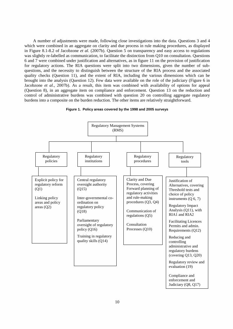
A number of adjustments were made, following close investigations into the data. Questions 3 and 4
which were combined in an aggregate on clarity and due process in rule making procedures, as displayed
in Figure 8.1-8.2 of Jacobzone et al. (2007b). Question 5 on transparency and easy access to regulations
was slightly re-labelled as communication, to facilitate the distinction from Q10 on consultation. Questions
6 and 7 were combined under justification and alternatives, as in figure 11 on the provision of justification
for regulatory actions. The RIA questions were split into two dimensions, given the number of sub-
questions, and the necessity to distinguish between the structure of the RIA process and the associated
quality checks (Question 11), and the extent of RIA, including the various dimensions which can be
brought into the analysis (Question 12). Few data were available on the role of the judiciary (Figure 6 in
Jacobzone et al., 2007b). As a result, this item was combined with availability of options for appeal
(Question 8), in an aggregate item on compliance and enforcement. Question 13 on the reduction and
control of administrative burdens was combined with question 20 on controlling aggregate regulatory
burdens into a composite on the burden reduction. The other items are relatively straightforward.
Figure 1. Policy areas covered by the 1998 and 2005 surveys
Regulatory
policies
Regulatory
institutions
Regulatory
procedures Regulatory
tools
Explicit policy for
regulatory reform
(Q1)
Linking policy
areas and policy
areas (Q2)
Central regulatory
oversight authority
(Q15)
Inter-governmental co-
ordination on
regulatory policy
(Q18)
Parliamentary
oversight of regulatory
policy (Q16)
Training in regulatory
quality skills (Q14)
Clarity and Due
Process, covering
Forward planning of
regulatory activities
and rule-making
procedures (Q3, Q4)
Communication of
regulations (Q5)
Consultation
Processes (Q10)
Justification of
Alternatives, covering
Threshold tests and
choice of policy
instruments (Q 6, 7)
Regulatory Impact
Analysis (Q11), with
RIA1 and RIA2
Facilitating Licences
Permits and admin.
Requirements (Q12)
Reducing and
controlling
administrative and
regulatory burdens
(covering Q13, Q20)
Regulatory review and
evaluation (19)
Compliance and
enforcement and
Judiciary (Q8, Q17)
(Q8, Q17)
Regulatory Management Systems
(RMS)

11
These dimensions correspond to the full 2005 database. A table of correspondence is presented below
which presents also the mapping with the 1998 data.
Table 1. List of policy areas of 2005 and 1998 surveys
N° Questions Titles Titles 98-05
1 Q1 EXPL_POL Adoption of explicit policy for regulatory reform.
Figure 1,
Yes
2 Q2 COHER Policy coherence integrating competition and market
openness Figure 2.1-2.2,
Yes
3 Q3&Q4 CLAR_PROC Clarity & due process in rule-making procedures
Figure 8.1-8.2,
Yes
4 Q5 COMMUNI Communication of Regulations. Easy Access
Figure 10,
Yes
5 Q6&Q7 JUSTIF_ALTER Provision of justification for regulatory action, search for
alternatives Figure 11,
Yes
6 Q8/Q17 COMPL_ENFOR Compliance, enforcement and judiciary Figure 16.1 and
figure 6.
Yes
7 Q10 CONSULT Consultation processes Figure 9, Yes
8 Q11 RIA_PROCESS Assessing the quality of new regulation through RIA 1
Figure 12-1, Explicit RIA processes,
Reduced to
1 var.
9 Q11 RIA_EXTENT Assessing the quality of new regulation through RIA 2
Figure 12-2, Extent of RIA processes
No
10 Q12 FACIL_LICEN Facilitating licences, permits and administrative
requirements Figure 14.1, 14.2,
Yes
11 Q13&Q20 REDUC_BURD Reducing and controlling administrative and regulatory
burdens Figure 13.1, 13.2, 13.3,
Yes
12 Q14 TRAINING Training in regulatory quality skills Figure 7.2, Yes
13 Q15 INSTIT_CAP Institutional capacity for managing regulatory reform
Figure 3.2,
Yes
14 Q16 PARLIAM Parliamentary oversight of regulatory policy Figure 5, No
15 Q18 LEVEL_GVT Multi-level co-ordination mechanisms for regulatory
policy Figure 4,
No
16 Q19 REVIEW-EVAL Dynamic process of evaluation and update of regulations
Figure 15.1, 15.2
Yes
Note: all figure numbers are from the publication Jacobzone et al. (2007b).
The 2005 data was linked to the 1998 data, albeit for a more limited number of variables. In the 1998
data sets, the parliamentary aspects, multi level regulatory governance were not addressed. RIA was also
analysed in a way that does not offer the possibility of constructing two separate variables, as the details on
the extent of the tests involved in the RIA processes are missing As a result, three policy areas do not
appear in 1998 and the 1998 data covers 13 dimensions for 27 countries.1 Data in 2005 was also often
richer and more detailed for the same variables. As a result, for many of the existing dimensions, the
composite indicators that are linked for 1998 and 2005 are constructed on a sub-set of data. Therefore,
three data sets will be considered for the analysis:
the full 2005 database (2005 data);
the 2005 linked database (sub-set of the 2005 database that is linked to the 1998 data);
the 1998 database (1998 data).

12
The main element of the grouping above is to present together meaningful dimensions of regulatory
policy, building on the previous analysis (Jacobzone, 2007b). The steps that will be followed for the
purpose of mapping of these dimensions involve:
an overview of the correlation between the variables;
a discussion and interpretation of the results from the principal component analysis. The
presentation includes technical aspects as well as a policy-oriented discussion of the results.
Analysis of the correlation between the variables
A detailed analysis of correlation is a prerequisite for performing factor analysis. The results generally
show that about 85% of the time, the correlations are positive (see Tables A1.1, A1.2, A.3, Correlations).
This means that countries which perform well for one category of systems of for regulatory management
are more likely to perform well for others as well.
Strong correlation appears between Institutional Capacity and the existence of a formal regulatory
policy. These are also linked to training, compliance and enforcement, as well as the structure and extent of
the RIA process. This is consistent with the OECD analysis and message that the role of Regulatory
Oversight Bodies is crucial to ensure core aspects of regulatory quality, including regulatory impact
analysis. A number of variables are also related that touch upon processes for preparing new regulations.
These include consultation, which is closely related to the search for alternatives, as well as RIA and
mechanisms for co-ordination across levels of government. Similarly communications in terms of easy
access to regulations is linked to clarity and due process in regulatory procedures, as well as to alternatives.
These variables link core aspects of a high quality regulation framework, with tools such as RIA, easy
access to regulation through communication with capacity for high quality regulation with a central
oversight body, training and co-ordination across levels of government.
The aspects on facilitating licences and permits, which reflect administrative simplification policies,
tend to not be correlated with other elements. They are even sometimes slightly negatively correlated with
consultation, training or clarity and due process, which will be explained by further analysis. Policies for
burden measurement and reduction are weakly but positively correlated to facilitating licences and permits
and are positively correlated to all variables which distinguish them from the other administrative
simplification policies.
The variables on policy coherence, linking regulatory policy and management to other policy areas in
terms of competition and trade, are only related to rule making procedures but not to the other aspects.
The patterns are generally confirmed in the 2005 linked dataset, which is a subset of the above, even
if there are slightly stronger negative correlations at times. For 1998, things are slightly different. The main
patterns involve links between the variables focused on the processes for preparing new regulations,
(consultation, justification and alternatives, RIA) and variables such as communication and easy access to
regulations, as well as institutional capacity and training. The variables on policy coherence and explicit
regulatory policy were less strongly linked then, except with institutional capacity. The facilitation of
licences and permits was positively correlated with clarity and due process, and more strongly and
negatively correlated then with compliance, enforcement and policy coherence. These results will be
understood better in the context of the graphical depiction below. Burden reduction was also a policy area
not correlated with others. At that time, policies for review evaluation and update were more closely
related to RIA, institutional capacity, as well as to consultation, clarity and due process as well as
communication and easy access. This may also reflect the specific emphasis in earlier days of regulatory
reform on stocktaking and full reviews of the regulatory stock, as experienced by a number of countries.

13
The principal component approach
Number of Principal Components retained
The factor analysis involves a Principal Component Approach (PCA). The variables that reflect the
various policy areas are first evaluated according to their contribution to the overall variance in the data,
and then grouped according to each of the principal components. One of the key aspects is to understand
how many principal components can help structure the dataset. Since the 16 variables are combined to a
smaller number of principal components, this will reduce the information, while offering the benefit of
some form of tractable analysis. Therefore there is a trade-off between obtaining a parsimonious and easily
interpretable dataset on the one hand and saving as much information as possible on the other hand.
The amount of additional information provided by a principal component equals the percentage of the
datasets total variance explained by this component. This percentage in turn depends on what is called the
Eigenvalue.2 The principal components are therefore numbered in descending order according to their
Eigenvalues. A standard approach is to keep all principle components with Eigenvalues above 1, which in
the current case in all the factor analysis for the first four components. These four components will be used
when computing aggregate composites for the purpose of regressions.
Another criterion is also the share of the total variance explained and also in relation to the policy
relevance of the principal component. Under this approach, the first four components represent
approximately two third of the total variance of the dataset in each of the analyses, while the first two
already include close to half of the total variance (Table 2 below). More detailed descriptive analysis will
therefore be undertaken on the first two components below.
Table 2. Eigenvalue and share of total variance explained by the principal components
2005 data 2005 linked data
Principal component
Eigen value
Percentage of variance explained
Total cumulated
percentage of variance
explained
Principal component
Eigen value
Percentage of variance explained
Total cumulated percentage of variance explained
1 5.98 37.4 37.4 1 3.69 28.4 28.4
2 1.85 11.5 48.9 2 2.24 17.3 45.6
3 1.65 10.3 59.2 3 1.48 11.4 57.0
4 1.17 7.3 66.5 4 1.25 9.6 66.6
1998 data
Principal component
Eigen value
Percentage of variance explained
Total cumulated percentage of variance explained
1 4.37 33.6 33.6
2 1.87 14.4 48.0
3 1.38 10.7 58.7
4 1.19 9.1 67.8

14
Regulatory Policy Management in 2005: two core dimensions
This section describes and interprets the principal components, which were retained for the purpose of
the PCA. The focus is on the first two components since they are more easily interpretable and contain the
most information. The full first four components are presented in the Annex (Tables A1.4, A.1.5, A.1.6)
The goal is to provide some relevant policy oriented interpretation of the information provided by the
components. The variables that contribute strongly to the construction of each principal component will be
listed together with their relative contributions.
The results of the correlations can help anticipate the patterns derived from the PCA. These show a
clear link between the different dimensions of regulation. Generally countries strongly involved in certain
areas of regulation also tend to be strongly involved in others. For example countries providing formal
training programs for regulation skills are also much more likely to conduct regulatory impact analysis and
have strong capacity for regulatory reform. There is a group of regulatory indicators for which such a
mutually supportive dynamic is especially strong. This group includes such areas as:
the existence of procedures for communicating regulations;
conducting of regulatory impact analysis;
having a dedicated body for promoting regulatory policy;
providing training in regulatory skills;
the existence of formal mechanisms for intergovernmental co-ordination.
These are related to the existence of strong regulatory institutions and tools as well as regulatory
capacity building. The strong positive correlations among these regulatory indicators as well as their
positive correlations with the other indicators lead to the hypothesis that there may be positive externalities
linked to setting up an effective institutional framework for regulation and developing tools and capacities
for good regulation. All of this is reflected in the first axis of the analysis.
First component: Institution, Tool Capacity Building (ITC QREG)
The first component driven by the Factor Analysis was named Institution, Tool and Capacity building
(ITC QREG), as this generic term reflects the contribution of the key variables of quality regulation to this
axis. This component regroups the variables that are closely related, and may provide overlapping
information, into single principal components
The variables that contribute strongly to the construction of each principal component are listed
together with their relative contributions that are expressed in terms of co-ordinates in the table below. The
contribution concerns the percentage that a certain variable contributes to the construction of a component.
The co-ordinates concern whether a variable correlates positively or negatively with a principal
component. A stronger positive correlation will translate into numerically higher positive co-ordinates.
This first component represents 37% of the total variance, showing the importance of these grouped
variables. This is consistent with ²what is known among statisticians as the “Gutman effect”. In a dataset
where mainly positive correlations exist among variables, the first principal component will often represent
these correlations. This means that the variables which are most strongly positively related with the dataset
will have the strongest contributions to the principal component and that all variables are going to have
positive co-ordinates, as is the case with the current dataset.

15
This is the first and most significant principal component. It explains more than a third of the total
variance, i.e. the information within the dataset. This component provides further evidence on the
importance of what has been noted as part of the correlation analysis: the mutually supportive dimensions
of a strategy for regulatory quality, mainly focused on setting up an appropriate institutional framework
and assessing the quality of new regulations through appropriate tools. “ITC Q REG effect” (see
correlation analysis). The variables below relate to RIA, consultation, institutional and parliamentary
oversight, multi level aspects and procedures. The variables that form the core of this “IT effect”3 are the
ones contributing most strongly to the construction of this component. Since they all have positive co-
ordinates, the countries that appear on the positive side of this axis will be those that have most widely
adopted such practices.
Table 3. Component 1 – “Institution, Tool, Capacity Building”, 2005 data
Variable Contribution Co-ordinates
RIA_EXTENT Assessing the quality of new regulation through RIA (extent of coverage)
11.8 0.84
JUSTIF_ALTER Provision of justification for regulatory action, search for alternatives
10.1 0.78
LEVEL_GVT Multi-level co-ordination mechanisms for regulatory policy
9.2 0.74
RIA_PROCESS Assessing the quality of new regulation through RIA (RIA process)
8.5 0.72
COMPL_ENFOR Compliance, enforcement and judiciary 8.4 0.71
TRAINING Training in regulatory quality skills 8.3 0.7
INSTIT_CAP Institutional capacity for managing regulatory reform
8.2 0.7
CONSULT consultation 6.7 0.64
PARLIAM Parliamentary oversight of regulatory policy 6 0.6
CLAR_PROC Clarity & due process in rule-making procedures 5.7 0.58
REVIEW_EVAL Dynamic process of evaluation and update of regulations
5.7 0.58
COMMUNI Communication of Regulations. (easy access) 5.4 0.57 Note: See full detail of the axis in Table A1.4. The contribution is the percentage of the variance explained. The coordinate corresponds to the factor loading.
Second Component – Stock Oriented Strategies, Simplification (SOSS)
The second component produced by the Factor Analysis represents in turn only 11.5% of the total
variance. The variables that are positively correlated with this component involve “Facilitating Licences
and Permits”, “Explicit Regulatory Policy”, “Evaluation Review and Update” and “Burden Reduction” to a
lesser extent. This is consistent with corrective strategies aimed at administrative simplification, burden
reduction and ex post review of regulations. These policies are also often supported by explicit policies for
regulatory reform and administrative simplification.
However, some variables contribute negatively to this axis, including “Policy Coherence” and
“Clarity and due process”. This may only reflect that those countries with a key emphasis on
simplification, evaluation review and burden reduction, may also at the same time have less integrated
regulatory policies, and less attention to due process. More detailed analysis of the variables with negative
co-ordinates on this axis also involve communication and easy access to regulations, search of alternatives,
consultation, extent of RIA processes and training. Clearly this means that countries that may be located on
the positive side of this axis SOSS, may have less developed strategies for regulatory quality in terms of
their new regulations, reflecting maybe a different stage in regulatory reform.

16
Table 4. Component 2 – Stock Oriented Strategies, Simplification (SOSS), 2005 data
Variable Contribution Co-ordinates
FACIL_ LICEN
Facilitating licences, permits and administrative requirements
28.5 0.73
COHER Policy coherence integrating competition and market openness
12.9 -0.49
CLAR_ PROC
Clarity & due process in rule-making procedures
12.6 -0.48
EXPL_ POL
Adoption of explicit policy for regulatory reform.
10.2 0.43
REVIEW_ EVAL
Dynamic process of evaluation and update of regulations 9.9 0.43
REDUC_ BURD
Reducing and controlling administrative and regulatory burdens
9.7 0.42
Note: See full detail of the axis in Table A1.4. The contribution is the percentage of the variance explained. The coordinate corresponds to the factor loading.
These results show that in 2005 two very different approaches to regulation were chosen by OECD
countries, with countries focused on capacity, ex ante assessment and consultation on the one side, and
other countries focusing more on simplification and burden reduction strategies. This will serve when
mapping groups of countries through the factor plans, with the next step of the analysis below.
Complementary elements from the 2005 reduced sample
The results are consistent with the full sample, even if they are slightly less clear cut, with a first axis
mainly structured around alternatives (19.6%), RIA (16.4%), clarity and due process (13.8%),
communication and easy access to regulations (9.2%), policy coherence (8.8%). This time the review and
evaluation, also comes in (7.6%), with institutional capacity (7.4%) and training (6%). The message
remains therefore broadly the same (see Table A1.5 for full details).
Similarly the second axis involves an explicit regulatory policy (22.4%), facilitating licences and
permits (20%), policy coherence (10.7%), institutional capacity (8.5%), and burden reduction (6.6%).
However in this 2005 linked sample fewer questions were available on burden reduction, as they are
consistent with the 1998 questionnaire. The fact that institutional capacity and policy coherence appear
positively is dimmed by the fact that consultation (6.8%), training (14.3%), and communication and easy
access to regulation (6.7%) all appear negatively correlated with this axis. It is still mainly consistent with
a focus on regulations ex post, with a strong policy, but a less clear cut strategy for the rest.
Regulatory Policy Management in 1998: broadly similar patterns
In the 1998 data, the first axis represented a third of total variance (33.6%), and the second about a
seventh (14.4%). The first component is still consistent with an “Institution, Tool, Capacity Building
Effect”. The variables are all positively correlated and supportive, including RIA, consultation, training,
institutional capacity, clarity and due process and communication. The only major difference is the fact
that the “Review evaluation and update” of regulation had a much greater contribution to this axis,
reflecting perhaps the fact, that, in early steps of regulatory reform, this wider emphasis on the review of
the stock and update was part of the core general strategy (see Table A1.6 for full details).

17
Table 5. Component 1 – “Institution, Tool, Capacity Building”, 1998 data
Variable Contribution Co-ordinates
RIA Regulatory Impact Analysis 15.7 0.83
JUSTIF_ ALTER
Provision of justification for regulatory action, search for alternatives
14.9 0.81
REVIEW_ EVAL
Dynamic process of evaluation and update of regulations
13.8 0.78
CONSULT Consultation 12.5 0.74
TRAINING Training in regulatory quality skills 12.4 0.74
CLAR_ PROC
Clarity & due process in rule-making procedures
10.9 0.69
COMMUNI Communication of Regulations. (easy access)
8.8 0.62
INSTIT_ CAP
Institutional capacity for managing regulatory reform
7.2 0.56
Note: See full detail of the axis in Table A1.6. The contribution is the percentage of the variance explained. The coordinate corresponds to the factor loading.
However, the patterns are slightly different in terms of the second axis. The burden reduction variable
is below the 5% contribution threshold. The main variable is the “facilitating licences” variable, which has
the strongest contribution, and is also positively correlated with due process. The second contribution,
corresponds to compliance and enforcement, and is negatively correlated with the former. The main
conclusion is that this axis is still weakly consistent with a focus on administrative simplification, but that
the countries which are strong in terms of efforts to facilitate licences and permits are also scoring less well
in terms of policy coherence.
Table 6. Component 2 – Administrative simplification, due process 1998 data
Variable Contribution Co-ordinates
FACIL_ LICEN
Facilitating licences, permits and administrative requirements
36.6 -0.83
COMPL_ ENFOR
Compliance and Enforcement 29.8 +0.75
CLAR_ PROC
Clarity & due process in rule-making procedures
11.2 -0.46
COHER Policy coherence integrating competition and market openness
5.5 +0.32
Note: See full detail of the axis in Table A1.6. The contribution is the percentage of the variance explained. The coordinate corresponds to the factor loading. The graphical depiction was inverted for the second axis, so that the countries in the upper part of the chart do reflect higher scores on the variables for facilitating licences.
Typologies of country approaches to regulatory quality in 1998 and 2005
The principal components identified by the can be represented in a graphical way as axes. When
combining two principal components using one as the horizontal axis and the other as the vertical axis one
obtains a two-dimensional factor plan. The countries can then be projected onto the plan. This allows one
to see the countries characteristics, as measured by the two principal making up the factor plan. The factor
analysis also provides the co-ordinates of the countries against those axes. As a result, it helps to identify a
typology, grouping countries according to their relative approaches towards regulatory reform. The
analysis will first proceed with the 1998 data, before turning to 2005, and drawing the lessons from
countries move and progress over the period.
18
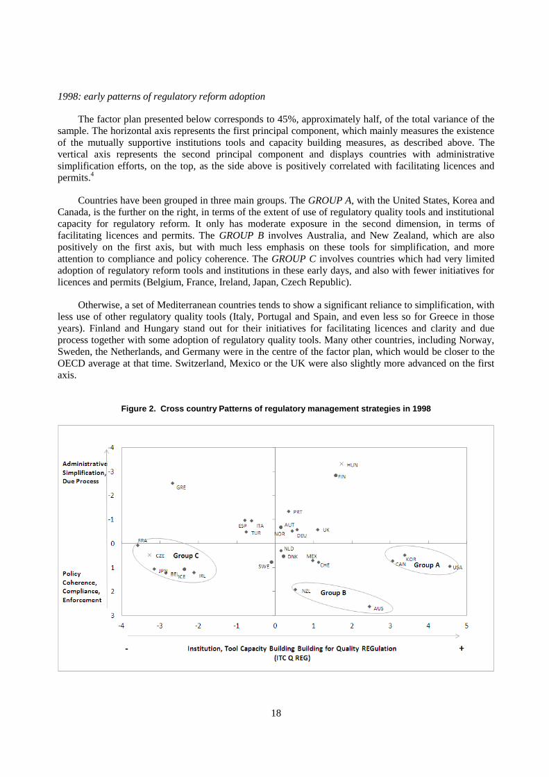
1998: early patterns of regulatory reform adoption
The factor plan presented below corresponds to 45%, approximately half, of the total variance of the
sample. The horizontal axis represents the first principal component, which mainly measures the existence
of the mutually supportive institutions tools and capacity building measures, as described above. The
vertical axis represents the second principal component and displays countries with administrative
simplification efforts, on the top, as the side above is positively correlated with facilitating licences and
permits.4
Countries have been grouped in three main groups. The GROUP A, with the United States, Korea and
Canada, is the further on the right, in terms of the extent of use of regulatory quality tools and institutional
capacity for regulatory reform. It only has moderate exposure in the second dimension, in terms of
facilitating licences and permits. The GROUP B involves Australia, and New Zealand, which are also
positively on the first axis, but with much less emphasis on these tools for simplification, and more
attention to compliance and policy coherence. The GROUP C involves countries which had very limited
adoption of regulatory reform tools and institutions in these early days, and also with fewer initiatives for
licences and permits (Belgium, France, Ireland, Japan, Czech Republic).
Otherwise, a set of Mediterranean countries tends to show a significant reliance to simplification, with
less use of other regulatory quality tools (Italy, Portugal and Spain, and even less so for Greece in those
years). Finland and Hungary stand out for their initiatives for facilitating licences and clarity and due
process together with some adoption of regulatory quality tools. Many other countries, including Norway,
Sweden, the Netherlands, and Germany were in the centre of the factor plan, which would be closer to the
OECD average at that time. Switzerland, Mexico or the UK were also slightly more advanced on the first
axis.
Figure 2. Cross country Patterns of regulatory management strategies in 1998

19
In 2005, the first axis has broadly a similar significance, but with more variables contributing to an
enhanced notion of capacity building and tools. The second axis is also clearer cut, in terms of combining
administrative simplification and burden reduction strategies.
Three main groups have been identified. GROUP B involves Canada, Korea, but with the UK this
time. This group is the most advanced on the first axis, in terms of recourse to regulatory quality tools and
institutional set up, while also developing policies for administrative simplification and burden reduction.
GROUP C, including the United States, Australia, New Zealand, as well as Poland and Switzerland, is
relatively advanced in terms of use of regulatory quality tools, RIA, consultation, but is not prone to the
use of administrative simplification strategies and burden reduction. GROUP A on the contrary involves a
larger set of countries that have adopted a strategy for regulatory reform clearly aimed at simplification,
including Mediterranean countries, France, Italy, Spain, Portugal and Greece. Mexico is also in this group
and is slightly more advanced in terms of regulatory quality tools, mainly due to its adoption of RIA. The
positive side of this axis also involves less policy coherence and less clarity in rule making procedures,
which may also reflect some of the fragmented nature of regulatory policy in some of these countries.
Luxembourg is in this group the country with less recourse to tools and institutional set up.
Figure 3. Cross country patterns of regulatory management strategies in 2005
AUS
AUT
BEL
CAN
CZE
DNK
FIN
FRA
DEU
GRE
HUN
ICE
IRL
ITA
JPN
KOR
LUXMEX
NLD
NZLNOR
POL
PRT
SVK
ESP
SWE
CHETUR
UK
USA
EU
-3
-2
-1
0
1
2
3
-6 -4 -2 0 2 4 6
+
-
Stock Oriented Strategies forSimplification
Institution Tool Capacity building for Quality REGulation (ITC Q REG) +-
Group A
Group B
Group CNordic Countries

20
Apart from these main groups, Iceland is overall the country that had less developed regulatory
quality tools and institutions, below Luxembourg. The new EU countries, including the Slovak Republic,
the Czech Republic and Hungary also tended to have less developed quality tools on average, while this
was not the case for Finland, and also to rely comparatively less on administrative simplification and
burden reduction.
However, this second axis is also negatively correlated with coherence and clarity in rule making
procedures. This implies that the countries that are below on this axis do in fact score high on coherence
and clarity in rule making procedures, while those on the top may not. This may also explain why Nordic
countries, such as Sweden, first, but also Finland, Norway and Denmark, all score high in the bottom,
which can also positively reflect their search for coherence and clarity, given their consensus driven
culture. Germany was very close to OECD average in that 2005 year.
These results show interesting trends between 1998 and 2005, in terms of countries developing and
implementing various aspects of regulatory reform, strengthening their regulatory management systems
framework. This overview will now be complemented by a set of correlations assessing the links between
overall regulatory management policies, as well as main policies as expressed through the first two
components of these factor analyses, in relation to external factors and data measuring governance, quality
of doing business framework, product market regulation and competitiveness.

21
II. TESTING HOMOGENEITY AND CONSISTENTY OF REGULATORY MANAGEMENT
SYSTEM INDICATORS WITH EXTERNAL INDICES
This section will rely on results from the previous section to analyse the correlations and links
between the OECD RMS indicators and external available indices. This involves correlation analysis in
order to assess the robustness of the RMS indicators and the strength and direction of possible linear
relationships between the RMS and other external indices. Identifying associations between these
indicators can improve understanding of how various dimensions of regulatory management systems
quality can relate to externally measured features of competitiveness, quality of doing business
environment or governance. The section will briefly introduce the indicators used for the analysis, both in
terms of OECD and external indicators, before turning to the results from correlation tests.
The indicators used for the correlations
External indicators
The current choice of indicators selected below is the result of a selection based on the availability of
these indicators and their relevance to the issue of regulatory quality management. Given some of the
international debates in the field, it does not imply either a positive or negative judgement on the intrinsic
value of these data in the perspective of good governance and development. Simply, those indicators exist
and are widely used. Therefore, they are a reference for policy assessment in a number of countries. In
some cases, as they rely on perception surveys, they may be felt as less “robust” than some of the OECD
indicators, which are reflecting institutional features. However, they are also addressing some of the
dimensions that are of importance for policy makers, as they also relate to outcomes, or results, either in a
way that reflects business perceptions, or some more simple but objective measures of regulatory burdens,
such as the number of days to open a business.
The data used for the correlations include the following set of external indicators:
Doing Business Indicator (DBI)
The Doing Business database is managed by the World Bank5 and provides objective measures of
business regulations and their enforcement, based on surveys from experts and private sector consultants
around the world. The database is structured along a number of core dimensions illustrating the regulatory
costs of business. The 2005 edition includes a methodological note on the construction (measuring with
impact), showing their filiations with some early work of De Soto The Other Path, on a time and motion
study to show the obstacles to establishing a business in Peru. These dimensions may have varied over the
years. In 2005, this study covered 145 countries, and was structured across the issues of:
starting a business;
hiring and firing workers;
registering property;
getting credit;
protecting investors;
enforcing contracts;
closing a business.

22
These data have often had a significant impact on the domestic debates in many countries. Many of
the countries' efforts at cutting red tape have been sometimes related to some of the dimensions illustrated
in that work. More details can be found in Annex.
The data used for the OECD study involve the aggregate overall score, the dimension 1, with its sub-
categories on procedures, time, the dimension 2 on dealing with licences, including number of procedures
and days, the employing of workers overall rank (dimension 3), the registration of property (dimension 4),
and the closing of a business (dimension 10).
Table 7. Doing Business indicators for the correlations (DB)
DB05 (-) Ease of doing business rank in 2005
DB05_SB (-) DB05 : Starting a business rank
DB05_SBProcedures (-) DB05 : Starting a business (Number of procedures)
DB05_SBTime (-) DB05 : Starting a business (Time in days)
DB05_DL (-) DB05 : Dealing with licences rank
DB05_DLProcedures (-) DB05 : Dealing with licences (Number of procedures)
DB05_DLTime (-) DB05 : Dealing with licences (Time in days)
DB05_EW (-) DB05 : Employing workers rank
DB05_RP (-) DB05 : Registering property rank
DB05_CB (-) DB05 : Closing a business rank
Note: (-) = Lower the better (+) = Higher the better.
These indicators are, to some extent, complementary to OECD RMS indicators. For instance, through
“dealing with licences”, the DB indicator determines if the regulatory environment promotes the operation
of business. Licences are assessed by the RMS in the context of how much efforts government are making
for reducing and streamlining them.
Global Competitiveness Index (GCI)
The World Economic Forum publishes annually the Global Competitiveness Report which includes
the Global Competitiveness Index6 to measure the group of institutions, policies and factors that are
thought to encourage sustainable current and medium-term levels of economic prosperity. This index is
very broad and it includes over 90 variables, of which two thirds come from the Executive Opinion Survey
and one third comes from publicly available sources. The Executive Opinion Survey relies on a network of
private sector executives which provides perception data on the quality of the business environment.
The correlations have included the main general competitiveness index, which is a composite of many
dimensions. The analysis also included the score and rank on institutions, the sub-index on burden of
government regulation, as part of “government inefficiency”, as measured by the executive opinion survey.
It also includes the pillar on market efficiency, with the corresponding score, which reflects product market
competition among others, and the sub-index on the efficiency of the legal framework, including the
settlement of disputes and the challenge of government actions and/or regulations.

23
Table 8. Global Competitiveness Indicators for the correlations (GCI)
GCI05 (-) Global competitiveness index rank in 2005
GCI05_Institutions (+) GCI05 Score : Institutions
RGCI05_I (-) Rank of GCI05_Institutions
GCI05_Inst_Burden (+) GCI05 Score : Institutions > Burden of government regulation
RGCI05_IB (-) Rank of GCI05_Inst_Burden
GCI05_Markets (+) GCI05 Score : Market efficiency
RGCI05_M (-) Rank of GCI05_Markets
GCI05_Mar_Legalframe (+) GCI05 Score : Market efficiency > Efficiency of legal framework
RGCI05_ML (-) Rank of GCI05_Mar_Legalframe
(-) = Lower the better. (+) = Higher the better.
This Global Competitiveness Indicator provides information about the capacity of regulatory systems
to promote private sector development, and to promote or inhibit competition. It also reflects a private
sector perspective based on perception data.
Worldwide Governance Indicators (WGI)
The World Bank Worldwide Governance Indicators is a research project covering 212 countries over
the period 1996-2007. It covers six dimensions of governance, with a set of aggregated indicators
(Kaufmann et al., 2008). This includes the process according to which governments are selected,
monitored and replaced; the capacity of the government to effectively formulate and implement sound
policies; and the respect of citizens and the state for the institutions that govern economic and social
interactions among them.
The governance indicators reflect the statistical compilation of responses on the quality of governance
given by a large number of enterprise, citizen and expert survey respondents in industrial and developing
countries (35 data sources by 32 organisations). The individual data sources underlying the aggregate
indicators are drawn from heterogeneous survey institutes, think tanks, non-governmental organisations,
and international organisations.
For the purpose of the correlation, a general aggregate was built by summing up the various
dimensions. The level of aggregation of the full governance index makes it very general. Contrary to some
other scores, these scores reflect a higher performance when the levels are higher. The dimensions
considered for the OECD analysis include the Government Effectiveness, Regulatory Quality, the Rule of
Law and the Control of Corruption. The aggregation into these various dimensions is obtained by an
unobserved component model, based on underlying characteristics which are assumed to contribute to
these dimensions. The mixed nature of the various inputs renders difficult a full and direct tracking of the
sources to the results.
Table 9. World Governance Indicators for the correlations (WGI)
WGI_total (+) World governance index
WGI_GE (+) WGI : Government Effectiveness
WGI_RQ (+) WGI : Regulatory Quality
WGI_RL (+) WGI : Rule of Law
WGI_CC (+) WGI : Control of Corruption
(-) = Lower the better. (+) = Higher the better

24
The WGI are considered as a way to quantify some dimensions of governance that are relevant from
the perspective of regulatory quality. They are therefore related to Regulatory Management Systems which
provides indications on countries practices in relations to established OECD guidelines for quality
regulation and performance. The correlation will provide insights as to how the two approaches can be
related. It could be expected that good regulatory management practices could contribute to the quality of
the institutional framework, even measured through more indirect and statistical methods.
OECD Product Market regulation indicator (PMR) and Regulatory Reform Index (REGREF)
The OECD indicators of Product Market Regulation (PMR) provide a comprehensive and
internationally comparable set of indicators that measure the degree to which policies promote or inhibit
competition in product markets. Until now, they measure the regulatory and market environments in
OECD countries in 1998 and 2003 and are consistent across time.
The analysis has selected the overall indicator, in terms of product market regulation, as well as the
sub-index on Barriers to Entrepreneurship, which relates to licences permits, communication and
simplification of rules and procedures, administrative burdens for corporations, for sole proprietor firms
and for specific sectors, antitrust exemptions and legal barriers, as well as the administrative burdens on
start-ups.
Table 10. Global Competitiveness Indicators for the correlations (GCI)
PMR (-) Product Market Regulation Indicator
PMR_BE (-) PMR : Barriers to entrepreneurship
REGREF (-) Regulatory Reform Indicator
Note: (-) = Lower the better, (+) = Higher the better.
The OECD REGREF indicator examines regulatory reforms of member countries annually over the
period 1975-2003 for 21 OECD countries measuring restrictions on competition and private governance.
More specifically, this indicator summarises information on regulatory conditions, such as entry barriers,
public ownership, market structure, price control and vertical integration, in seven non-manufacturing
sectors: airlines, telecoms, electricity, gas, post, rail, and road freight. It is on a scale of 0 to 6 (from least to
most restrictive), and is the only OECD indicator of regulation with such an extensive time-series
component.
Both PMR and REGREF indicators provide information about the capacity of regulatory systems to
promote private sector development, and to promote or inhibit competition. They are built on similar
principles as the OECD indicators of regulatory management systems, but their coverage of economic
issues is different, broader for PMR, more specific for REGREF with the advantage of the yearly
availability. These indices are important since they have also been statistically found to be significant for
economic growth and productivity (Conway et al., 2006) in a number of OECD economic studies.7 Hence,
if the RMS indicators, or some of their component are statistically correlated to these indices, they can also
be expected to have a positive impact on economic growth, and broader economic outcomes.

25
OECD Regulatory Management System Indicators
The OECD indicators involve a set of four indicators. The first two are the value of the countries co-
ordinates on the first two axes. A high value will involve a country placed on the right side of the charts
above, with either a high use of tools, institutions for quality regulation, or a more intensive approach to
stock burden reduction (as in the 2005 data). In addition, two other indicators have been computed. The
first is a simple average of the various 13-16 dimensions of regulatory management system quality
analysed above. Each of the indicators is computed with the full 2005 sample, the 2005 sample restricted to
the linked data and the 1998 sample.
Table 11. OECD Indicators of Regulatory Management Systems
RMS1 RMS2
Indices which are calculated from the co-ordinates of the projections of the countries positions on the first two components of the Principal Component Analysis
RMS1 = ITCQ REG
RMS2 = Stock Oriented Strategies, Simplification
Ind_av Naïve aggregated index, by simple average of the 13 or 16 variables
Ind_ag
Index aggregated using the weights given to each variable by the Principal Component Analysis:
05
05lk
98
Broad 2005 sample
Linked reduced 2005 sample
1998 data sample.
The second is a more elaborated indicator built using weights derived from the Principal Component
Analysis (See detailed method in Annex). In fact, the two indicators built with weighted averages or with
equal weights are relatively similar. The first wave of the Product Market Regulation Indicators
constructed by the Economics Department in 2003 used weights from Principal Component Analysis
(Conway and Nicoletti, 2003) while some of the recent updates have limited themselves to simple average
weighted composites (Wölfl A. et al., 2009).
Results from the correlations
Correlation tests are performed to quantify the relationship between the various sets of indicators
presented above and the family of RMS indicators. The correlations are using Spearman correlations tests,
as the scale of ranks is ordinal and which present the interesting statistical property of allowing testing for
correlations of ranks, which simplifies the approach when various indicators are constructed through
different techniques. In addition, this offers a test of sensitivity, with a P Value shown in the tables in
Annex. A P Value of less than 0.10 (0.05) means that the correlations are significant at a threshold of 10%
(respectively 5%) (see Tables A1.7, A1.8, A1.9, A.10 in the Annex).
Doing Business
The results of the correlations with the Doing Business indicators are available for 2005 data only
(Table A1.7). They show that at an aggregate level, the main indicator that is positively correlated with the
Ease of Doing Business in general is the RMS1, or ITQ REG, which is a composite involving the use of
Institutions, Tools and Capacity Building for Quality regulation, including also consultation and RIA. This
core dimension reflects the thrust of the message of the OECD principles for quality regulation and
performance, in terms of regulatory management. Whether for the full sample, or the restricted sample
(RMS105lk), the correlation is significant and with the expected sign (negative, as to facilitate the Ease of
Doing Business). However, this is not the case for the aggregated indicators, which include many other
dimensions of regulatory quality.

26
The correlation is also significant, and with the wrong sign with regards to the second dimension of
regulatory management system, in terms of burden reduction. However, this needs to be interpreted with
caution: countries that have identified themselves as investing strongly in this dimension are active in
rolling out simplification programmes and cutting licences and permits. Generally, these countries, where
this activity is a priority, have made a diagnostic which acknowledges the fact that regulatory burdens
hinder their business activity, and that they need to take steps to reduce these burdens. Therefore, the
correlation could also imply that those countries with relatively more significant regulatory burdens are
also those which are pushing their regulatory management system quality efforts towards administrative
simplification and burden reduction.8
The other correlations found with doing business involves correlations with the expected sign for
ITCQ REG (RMS 1), in terms of reducing the time to start a business, or dealing with licences, or even
employing workers. No correlation is found for closing a business. The same effect is found for the
administrative simplification policies (RMS2) concerning the registration of property.
Global Competitiveness Index (GCI)
The results of the correlations with the GCI index exist for 1998 and 2005 data. Some correlations are
found, with the expected sign, for the global competitiveness index for 1998; and its component for
institutions (Table 12). However, the only RMS indicator for which this is true is for the first component,
with the ITC QREG effect. Correlations are negative but not significant with the aggregate indicators. A
slight negative correlation is also found with the second component, in terms of administrative
simplification and due process.
Table 12. Correlations of OECD RMS with World Bank Doing Business indicators
RMS1_98
RMS2 _98
IND_AV98
IND_AG98
GCI98 -0.42** -0.37* -0.22 -0.21
GCI98 0.03 0.06 0.28 0.29
27 27 27 27
GCI98_IN -0.35* -0.14 -0.13 -0.13
GCI98_Institutions 0.07 0.48 0.51 0.53
27 27 27 27
The results of the correlations for the 2005 data show the correlations with the expected sign only in
terms of market efficiency and for the first ITC Q REG of the OECD indicators of regulatory management
system's quality (Table A1.8). No effects are found with the aggregate or the second component with the
full data set. The second component with the linked data reflects correlations with the wrong sign,
confirming some of the points made above concerning doing business indicators.
Worldwide Governance Indicators (WGI)
The results of the correlations with the worldwide governance indicators are available for 1998 and
2005 data (Tables A1.9 and A1.10). Almost no correlation is found in the 1998 samples, except between
the subcomponent of the worldwide governance indicators on regulatory quality and the RMS1, which
reflects the ITC QREG effect. However, no correlations exist in the 2005 sample, except for correlations
with the wrong sign with RMS2, but only with its component computed with linked data. There, the
parsimony of the data available to compute this second component may require caution before further
interpretation.

27
Overall these results may bear on the relatively abstract nature of the WGI indicators, which are
computed through rather aggregate econometric methods and are more difficult to rely to concrete
dimensions of regulatory governance and management.
OECD Product Market Regulation and REGREF Indicators
The correlations can be computed with the 1998 PMR and REGREF indicators (Table 13 below).
Significant negative correlations, hence with the expected sign, are found both with the aggregate
indicators as well as the first component (RMS1), ITC Q REG effect, with the REGREF indicator. This
indicator is very important since it has been found in econometric regressions to be statistically significant
in terms of contributing to increasing long term economic growth. Expected correlations are also found but
only with the RMS1, main ITC Q REG effect with the overall PMR indicator for 1998 as well as its
component on Barriers to entrepreneurship. For the first time here, the second component of the RMS data,
RMS2, in terms of administrative simplification, was also correlated with lower product market
competition barriers in 1998.
Table 13. Correlations of OECD RMS indicators with PMR and REGREF indicators 1998
RMS1_98 RMS2_98 IND_AV98 IND_AG98
PMR_98 -0.38* -0.50*** -0.23 -0.22
PMR_98 0.05 0.01 0.24 0.27
27 27 27 27
PMR_BE98 -0.35* -0.28 -0.24 -0.23
PMR_Barriers to Entrepreneurship 98 0.07 0.16 0.23 0.26
27 27 27 27
REGREF_98 -0.46* 0.09 -0.52** -0.51**
REGREF_98 0.06 0.72 0.03 0.03
18 18 18 18
Some effects in terms of 2005 data are also found but they are less clear cut (Table 14 below). A
strong and significant correlation is found for the indicators computed on the linked data only with the
REGREF indicator. The RMS1, first component, is generally not significant this time. However, negative
effects, with the wrong sign are again to be found with the indicator reflecting administrative simplification
policies. This could be consistent with some of the findings presented above in terms of the significance of
administrative simplification policies. It should also be pointed that technically the PMR indicators relate
to 2003 data while the second RMS data point is for 2005.
RMS of year 2005 (RMS05) is only statistically correlated to REGREF indicator. The tested version
of the GCI, WGI are DBI indicators correspond to year 2005. However, PMR and REGREF indicator are
just available to 2003, so this table must be read carefully. Even if the information collected through 2005
survey is not statistically significant with most of the external indicators, its relation with GCI, DBI and
PMR has the expected sign.
The RMS linked indicator links 1998 and 2005 survey data, as it was explained in the first section of
this report (see Table 1). This indicator is statistically correlated to GCI, DBI, PMR and REGREF
indicators, and has the expected. RMS overall indicator is constructed by estimating a wide average of
1998 and 2005 datasets. The correlation test indicates that it is statistically correlated with REGREF
indicators. The coefficients signs are the expected, except for WGI. The RMS linked and the RMS overall
cover a longer period and are tested with the 2003 or 2005 waves of the external indicators depending on
their availability.

28
Table 14. Correlations of OECD RMS indicators with PMR and REGREF Indicators 2005
RMS1_05 RMS2_05 IND_AV05
IND_AG05 RMS1_05lk
RMS2_05lk
IND_AV05lk
IND_AG05lk
PMR_03 -0.20 0.27 -0.06 -0.03 -0.22 0.43** -0.03 -0.01
PMR_03 0.30 0.15 0.75 0.86 0.28 0.02 0.89 0.96
30 30 30 30 27 27 27 27
PMR_BE03 -0.20 0.36** -0.04 -0.02 -0.25 0.47** -0.02 -0.01
PMR_Barriers to Entrepreneurship
03
0.29 0.05 0.83 0.92 0.20 0.01 0.92 0.98
30 30 30 30 27 27 27 27
REGREF_05 -0.23 0.01 -0.31 -0.28 -0.35 -0.22 -0.44* -0.44*
REGREF_05 0.32 0.95 0.17 0.22 0.16 0.38 0.06 0.07
21 21 21 21 18 18 18 18
Finally, the additional point can be made that closer insights into the data tends to show that Mexico
and Turkey rank well according to the RMS indicators while they score less favourably on the WBI. GCI
and PMR indicators. Repeating the one-tailed correlation test excluding these two countries leads to a
significant correlation between the RMS indicators and all other indicators except the WGI.
Dynamic correlations with OECD Product Market Regulation and REGREF Indicators
The results for the variable RMS2, which embodies administrative simplification and burden
reduction policies were slightly puzzling from a cross sectional perspective. Many countries are cutting red
tape in order to improve their competitiveness. However, those countries which make the most efforts may
not, at a given point in time, get the best marks in terms of ease of doing business or impediments to
product market competition. For this reason, a dynamic perspective will be adopted to relate changes in
variables of competitiveness or restrictions to market competition, and intensity of country efforts over this
second dimension of the factor analysis, which reflects simplification and burden reduction policies.
Among the indicators available, the OECD product market regulation indicator and the REGREF
variable are the most consistent over time, given the methodological stability to construct them. The other
external indicators have been subject to some slight methodological change over time, which makes them
irrelevant for dynamic analysis. For this reason, the analysis will focus on this section on the REGREF
variable and the product market regulation indicator, with the restriction that REGREF is available for
slightly less countries, and that the trend measured covers in fact a shorter time period 1998-2003.
Graphical depictions in Annex tend to show some significant correlations between reductions in the
REGREF indicator, showing greater market competition, between 1998 and 2005, in relation either to the
level of the efforts at the end of the period (RMS2-05) or at the beginning (RMS2-98). The correlations are
less pronounced for product market regulation, with the caveat of a slightly different time period (see
Annex Figure 1 trends in product market regulation and administrative simplification policies).
This is also confirmed when analysing the significance of the correlation analysis, through bilateral
linear regressions (Table 15 below). The slopes are always negative and highly significant with REGREF,
explaining up to 30% of the variance with the 2005 dimension, and still negative, but less significant with
the PMR indicator, explaining between 3 and 9% of the variance. Additional correlations on the sub-index
on Barriers to Entrepreneurship of the OPMR indicator yield slightly more pronounced results than the
overall PMR indicator.
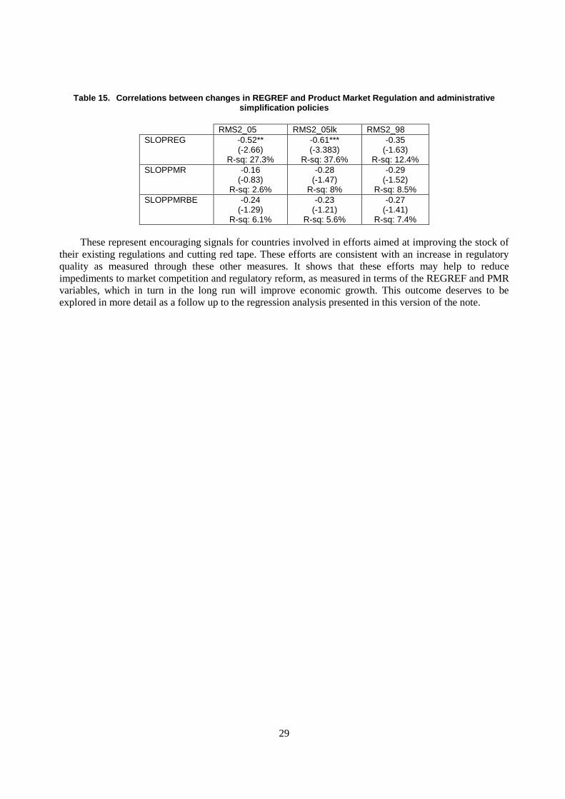
29
Table 15. Correlations between changes in REGREF and Product Market Regulation and administrative simplification policies
RMS2_05 RMS2_05lk RMS2_98
SLOPREG -0.52** (-2.66)
R-sq: 27.3%
-0.61*** (-3.383)
R-sq: 37.6%
-0.35 (-1.63)
R-sq: 12.4%
SLOPPMR -0.16 (-0.83)
R-sq: 2.6%
-0.28 (-1.47)
R-sq: 8%
-0.29 (-1.52)
R-sq: 8.5%
SLOPPMRBE -0.24 (-1.29)
R-sq: 6.1%
-0.23 (-1.21)
R-sq: 5.6%
-0.27 (-1.41)
R-sq: 7.4%
These represent encouraging signals for countries involved in efforts aimed at improving the stock of
their existing regulations and cutting red tape. These efforts are consistent with an increase in regulatory
quality as measured through these other measures. It shows that these efforts may help to reduce
impediments to market competition and regulatory reform, as measured in terms of the REGREF and PMR
variables, which in turn in the long run will improve economic growth. This outcome deserves to be
explored in more detail as a follow up to the regression analysis presented in this version of the note.

30
III. ASSESSING THE IMPACT OF SYSTEMS FOR THE MANAGEMENT OF
REGULATORY QUALITY FOR ECONOMIC GROWTH
Overview
This analytical work9 is designed to assess the relevance of regulatory management indicators for
economic policy. Regulatory management systems indicators have been constructed to reflect compliance
with good OECD principles for regulatory quality and performance. Therefore, a key issue is to assess
whether improvements in regulatory quality may influence macro-economic performance.
While quantifying the link between performance and regulatory quality involves significant technical
challenges, this report provides a first econometric attempt at quantifying the impact of improvements in
the RMS on a number of macro-economic outcomes. The analysis and methodology is constrained by a
paucity of observations, as only two waves of the RMS data were available until now.
The results of the regressions are suggestive but they need to be considered with caution due to the
paucity of data. Movement toward best-practice in the RMS unambiguously corresponds to improved
economic performance, along any of the dimensions that are measured. As a further robustness check, the
same regressions were run with the established Product Market Regulation (PMR) indicators,
corroborating inferences regarding the RMS. The apparent link between improved regulatory quality and
economic outcomes captured in these simple econometric models also highlights the value of the current
RMS survey being collected in 2008. With each additional year of survey data, the econometric
possibilities expand.
The analysis will first introduce the empirical model and strategies pursued, before turning to the
variables used to measure economic performance and the indicators of regulation and the results of the
regressions. All figures and tables are presented in Annex A1.
The modelling strategy
The modelling strategy uses the indicators of the Quality of Regulatory Management Systems, as
single aggregate variables. Existing models at the OECD have used the REGREF/PMR indicators to
establish a significant link between regulation and economic performance. The less frequent incidence of
the RMS indicators precludes their application in the model estimated with REGREF/PMR and glossed in
Box 2. Therefore, the econometric methods and specification are simplified and modified as appropriate to
fit the current context and data constraints.
In trying to isolate the impact of improvements in regulatory quality, per se, on economic
performance, it is important to control for factors that are unobserved or not measured by the
econometrician but correlated with both a country’s regulatory stance and labour productivity. Cross-
country heterogeneity has presented a significant obstacle to researchers seeking to quantify the link
between performance and different aspects of regulation, both inside the OECD and out. In most cases,
researchers are constrained by having a purely cross-sectional indicator that captures variation across
countries only for a single year. In a cross-sectional regression of performance on regulatory stance, the
coefficient on regulatory stance could absorb spurious idiosyncrasies across countries, and in the cross-
sectional context, fixed effects to control for this heterogeneity cannot be used. A large part of the
achievement in the previous OECD study (Conway et al., 2006) is the construction of a time series
beginning in the mid 1970s with the REGREF data for a cross-section of countries, permitting use of a
panel data methods, and particularly, inclusion of fixed effects to control for persistent, unobserved
individual heterogeneity across countries.

31
Box 2. The productivity growth “catch-up” model
The model of the previous OECD study (Conway, et al., 2006) uses the framework of Aghion and Howitt (2005) to relate labour productivity growth in a given country to productivity growth of the leader country as well as the difference in productivity levels between the country and the leader. Positive productivity shocks in the technology leader may stimulate growth in other countries, while “catch-up” suggests that countries situated at a greater distance from the productivity frontier would have greater scope for productivity improvements.
The previous study introduced the REGREF indicators into the Aghion and Howitt model to examine how regulation
and institutions might affect productivity growth, both directly, and indirectly by affecting the speed at which countries catch up to the productivity leader.
XTechGapPMRPMRTechGapLPLP leader )*()()ln(ln
where LP denotes labour productivity, TechGap is the „technological gap‟, and PMR denotes the appropriate indicator of product market regulation. X contains various control variables. Country, time, and industry-specific fixed effects are included to account for unobserved factors affecting productivity growth. Reflecting data availability, the model is estimated for a panel of 20 OECD countries over the period 1978 to 2003.
In the current RMS context, a proper time-series with yearly data is not available. Nonetheless, the
empirical strategy will be to construct a panel, making use of the limited time-series available The RMS
indicators are extended through time in two ways. First, a panel with time dimension T = 2 is created using
the Regulatory Quality Indicators that are available on a similar basis between the 1998 and 2005 survey
waves. Second, linear interpolation is performed on the RMS indicators from the 1998 and 2005 survey
waves to “fill-in” otherwise unmeasured regulatory quality between these years. Linear interpolation
requires the strong assumption that movement over time in regulatory stance follows a linear path, but has
the advantage of yielding additional years of data, bringing the total to T = 7 years. Using either the T = 2
or the T = 7 panels, since all variables vary over time, the model may be estimated using panel data
methods, such as Fixed or Random Effects, to control for unobserved individual heterogeneity. The
econometric difference and the relative significance of fixed versus random effects are explained in the
Annex.
A very simple model of performance outcome as a function of the relevant RMS indicator is
estimated using both fixed and random effects:
ititit RMSePerformanc )(
where i indexes countries, and t indexes years, and the error is treated differently, according to the
fixed or random effects context. Both methods may be considered to control for unobserved
individual heterogeneity, so that estimates of the model correspond to a per se effect of regulatory
quality on performance.
Fixed effects are typically the method of choice to estimate per se effects. However, fixed effects are
costly in terms of loss of degrees of freedom when the sample is small. In this context, random effects may
be more efficient. Random Effects estimation requires the assumption that the unobserved, time constant
portion of the error is uncorrelated with all explanatory variables for all periods. This assumption is not
likely to pose problems in the current context since no time constant regressors are included in the
specification. Random effects have the advantage of being more efficient, allowing identification of the
impact of regulation quality on performance with greater precision.10

32
A Hausman specification test is performed to determine the power of Random Effects estimates. This
tests the null hypothesis that the time constant component of the error is uncorrelated with all of the
explanatory variables at all time periods. Failure to reject the null may mean, inter alia, that estimates
using Fixed Effects and Random Effects are statistically similar enough that either method may be used to
estimate the model.11
In both fixed and random effects regressions, the Breusch-Pagan test for heteroskedasticity is
performed, and where appropriate, robust standard errors are employed. Additionally, while controlling for
possible endogeneity in the link between regulatory quality and performance is beyond the scope of this
report, the RMS indicators are lagged by one year, with respect to the performance variables, eliminating
the possibility of reverse causality between regulation quality and performance. Given the limited number
of observations, the model had to be kept as parsimonious as possible. It includes only the RMS indicator
on the right hand side as exogenous variables. This is in fact not too problematic, since fixed or
alternatively random effects will control for all other unobserved differences across countries that impact
performance.
Finally, each regression is re-estimated using the PMR indicators in place of the RMS indicators. To
the extent that the PMR indicators have been found to be significant in explaining economic performance
in more sophisticated, structural models, confirmation of the RMS results with the PMR indicators
strengthens the validity of the RMS estimates.
Data
Dependent Variables
The analysis below will consider four dimensions in terms of performance outcomes:
1. Total employment
The numbers of workers here are compiled with sample household surveys for all OECD countries
except for the United States where the source is the establishment survey. Total employment is defined as
the sum of civilian employment and members of the armed forces. Data from 1970 to 2006 were collected
from OECD Statistics, ADB database, Economic Outlook No 81.
2. Employment in the business sector
Employment in the business sector is the difference between total employment and employment in the
government sector. These data were compiled from OECD Statistics, ADB database, Economic Outlook
No. 81 for 1970 to 2006.
3. GDP, business sector
GDP volume in the business sector is calculated by subtracting the value added of the government
sector from total GDP. GDP was converted to a common currency using purchasing power parities (PPP)
for base year 2000 to make comparison across countries and time possible. The data were collected from
OECD Statistics, ADB database, Economic Outlook No. 81 for 1970 to 2006.

33
4. Labour productivity, business sector
Labour productivity for the business sector is defined as output per unit of labour input minus the
contribution of the government sector. These data are derived from OECD Statistics, ADB database,
Economic Outlook No 81 and are calculated as the ratio of GDP to total employment in the business
sector.
Exogenous variables of regulatory management quality
Two sets of variables are used in the regressions:
1. Regulatory management system indicators (RMS)
The regressions make use of RMS indicators from the 1998 and 2005 surveys These indicators
reflects compliance with OECD good practice for regulatory management system's quality, through a
number of components. The regressions were done using aggregate indicators covering all policy areas, or
sub-indexes mainly through the first (RMS1) and second component (RMS2) of the principal component
analysis. The aggregation is either done through a simple additive aggregate (RMS_av),12
or an aggregate
based on the weights of the Principal Component Analysis (RMS_ag). RMS1 reflects institutions, tools
and processes for quality regulation (ITC Q REG effect). The regressions with the second component
RMS2 are less conclusive and are not presented.
In addition, for all specifications, an interpolated version of the RMS is used to cover the entire period
1998 to 2006. This method makes the assumption that, on average and across countries, changes were
introduced gradually through the period. This has the econometric advantage of providing a much larger
sample of estimates, which helps to confirm the robustness of the coefficients and their validity. They are
shown on the right hand side of the tables.
2. Product Market Regulation Indicators (PMR)
The PMR indicator measures the degree to which policies promote or inhibit competition in areas of
the product market where competition is thought to be viable. The scale goes from least restrictive (0) to
most restrictive (6). These indicators, together with the associated REGREF indicator, have been found in
past OECD work to be econometrically significant in terms of economic growth.
Results
Fixed effect regressions
The regression results yield estimates of the impact of regulation management system quality on
economic performance measured in terms of total employment, total employment in the business sector,
GDP for the business sector and labour productivity. Where the null hypothesis of homoskedasticity was
rejected, robust standard errors were used, which is the case for all regressions, except with labour
productivity in the business sector as dependent variable. Generalizing across the different performance
variables and all specifications, the coefficient on the RMS indicators are of the expected sign and
statistically significant across the board. The coefficient on the relevant RMS indicator is significant at
either the 5% or the 1% level except in the case of the regression of business sector GDP on RMS1, of the
expected sign but not statistically significant, and of total employment on RMS1 and RMS_AV, which are
still statistically significant at the 10% level. When the interpolated variables are considered, significance
typically improves to attain the 1% level.

34
See Table A1.11. Fixed effect regressions with RMS1 indicator (simple/Interpol.)
See Table A.1.12. Fixed effect regressions with RMS simple average indicator (simple/Interpol.)
See Table A1.13. Fixed effect regressions with RMS weighted aggregated indicator (simple/Interpol.)
In these regressions, the coefficient on regulatory management quality is positive; an improvement in
regulatory quality corresponds to a statistically significant increase in total employment, employment in
the business sector, GDP for the business sector, and labor productivity for the labor sector.
Across methods and specifications, the R-square represent the residual share of the total variance in
the performance variables that can be explained by the regression on regulatory management system
quality indicators. As a result, they are low, but not surprisingly so given the paucity of data.
Random effect regressions
Random effect regressions have also been performed using the interpolated indicators with T = 7. In
all regressions other than the regressions of business sector GDP on RMS_AV and RMS_AV, the
Hausman accepts the null hypothesis that the individual effects are uncorrelated with the other (RMS)
regressors, indicating that the assumptions needed to apply random effects are satisfied, and both fixed
effects and random effects estimation produce valid results. This justifies presenting both sets of results in
the report. The important element is that coefficient estimates are generally robust across the
specifications.
In the random effects regressions, the R-square ranges from 1% to 6%. This is the percentage of the
total variance that could be solely explained attributed to differences in regulatory management system
quality.
See Table A1.14. Random effect regressions with interpolated RMS1 indicator
See Table A1.15. Random effect regressions with interpolated RMS_av indicator
See Table A1.16. Random effect regressions with interpolated RMS_ag
Product Market Regulation Indicators
Complementary results are obtained from identically specified fixed effects and random effects
regressions where the RMS indicators are replaced with the PMR indicator. These regressions use,
alternatively, the PMR at two points in time, 1998 and 2003, and the interpolated version.13
The negative
and significant coefficient on the PMR suggests that movement from less to more restrictive
product market regulation corresponds to improved performance along these same dimensions.
The coefficients are significant in all cases with the interpolated indicators, but only for labour
productivity in the non interpolated indicator and fixed effect model. The value of the coefficient
is the same for interpolated and simple indicator regressions.
See Table A1.17. Fixed effect regressions with PMR indicator (simple and interpolated)
See Table A1.18. Random effect regressions with interpolated PMR indicator

35
Summary
Overall, the regressions results yield some estimates of the impact of regulatory management system
quality on economic performance, controlling for countries' idiosyncratic characteristics. The results tend
to show that, while most of the cross country variance is explained by country specific characteristics, a
small share could be attributed to the impact of factors linked to the quality of regulations. While they are
not large in magnitude, these effects appear to be significant and systematic. This implies that an
improvement in regulatory quality corresponds to a statistically significant increase in total employment,
employment in the business sector, GDP for the business sector, and labor productivity for the business
sector.
36
IV. CONCLUSIONS
This report takes a first step forward in using the data of indicators of quality of Regulatory
Management Systems for analytical purposes. This follows a three-stage approach. First, a descriptive
analysis of the sample was done using Principal Component Analysis. Second, correlations were
performed linking information on systems for managing the quality of regulation with a set of other related
institutional variables on governance, ease of doing business and regulatory quality itself, from other
institutions as well as from the OECD PMR. Third, the RMS indicators together with the other OECD
PMR indicators were inserted in an econometric model with a goal of measuring the impact of systems for
the management of regulatory quality on economic performance.
The result of the correlations shows that generally the Doing Business, Competitiveness index are
correlated with the PMR and REGREF indicators with the expected signs. This might reflect the fact that,
when a country has a high-quality regulatory management system, its private sector and competition
environments and their business friendliness, as measured by GCI, DBI and PMR indicators, are
performing as well. In addition, investment in administrative simplification policies may translate in
additional improvements in terms of product market competition, with positive implications for economic
growth in the long term.
The correlations are also helpful to guide the econometric analysis. The correlations tend to indicate
that both the aggregate indicators, as well as the first component RMS1, with the ITC QREG effect, may
be the most relevant and robust RMS indicators to examine the impact of the quality of regulatory
management systems in terms of economic growth.
The regression analysis is constrained by the small sample size. Nonetheless, panel regressions were
performed, allowing control for idiosyncrasies across countries to isolate the per se effect of regulatory
management system quality. The results uniformly indicated a significant improvement in economic
outcomes (employment, GDP, labour productivity) in response to improvements in of the systems for
regulatory management. These results are also consistent with similar regressions using the established
PMR.
The finding of a statistically significant, positive link between systems for managing the quality of
regulation quality and economic performance suggests that further analysis could be desirable. Each future
wave of the survey on regulatory management systems will facilitate and strengthen the analytical base.
With proper time series, different and more sophisticated models can be envisaged, in the framework of
Aghion and Howitt (2005) to posit labour productivity growth in a given country as a function of
productivity growth of the leader country as well as the difference in productivity levels between the
country and the leader. The RMS indicators could then be introduced into the Aghion and Howitt model to
examine how the systems for managing the quality of regulation might affect productivity growth, both
directly, and indirectly by affecting the speed at which countries catch up to the productivity leader.
From a policy standpoint, while the scale and magnitude of the results can be disputed, they provide
consistent support for the economic benefits of systems for managing the quality of regulations. They help
to quantify some of the short term and long term effects that may occur when countries go through the
often painful processes of improving the quality of their regulations. This implies rigor, process, impact
assessment and often may be challenging in view of the constrained timing of the political agenda.
However, this may also result in an economic environment that is also conducive to the achievement of
greater prosperity, thus delivering results for citizens and businesses. The OECD can also add value to
national insights through its comparative perspective, taking advantage of the cross country and over time
variance that exist through the diversity of institutional and regulatory systems.

37
NOTES
1. Data are missing in 1998 for Luxembourg, Poland and Slovak Republic.
2. A mathematical term derived from the algebraic operations for calculating the explained variance.
3. As noted before, these are especially Intergov, RIA, Comm, Cenral and Skills.
4. This was to facilitate the coherence with the presentation of the 2005 results, as in the 2005 results, the
variables on facilitating licences and permits, as well as burden reduction, are positively correlated with
this axis.
5. See World Bank 2003, 2004, 2005, 2006, 2007, 2008.
6. See World Economic Forum (2007, 2008).
7. For a summary, see OECD (2008).
8. The effects are less clear cut concerning the linked data for the second dimension (RMS205lk), with
generally correlations with a positive side, reinforcing the analysis made above. None of the indicators at
aggregate level with the linked data only show any relevant correlations. This may reflect the restricted
nature of such indicators.
9. This analytical work has been undertaken with the contribution of Prof. Faye Steiner, Economics
Department, Stanford University, and Erika Lopez Ponton, University Paris I Sorbonne.
10. This is because random Effects estimation is a GLS (Generalized Least Squares) transformation in which a
fraction of the average over time of each variable is subtracted from it. The fraction depends on the
variance of the time-varying and time constant error components as well as the number of time periods in
the panel. Moreover, there is no loss of degrees of freedom since country fixed effects are not included.
11. Technical details on Fixed and Random Effects can be found in the technical Annex following this report.
12. Now adopted by the Economics Department for its 2007 Survey on Product Market Competition Indicators
(see Wölfl A. et al., 2009).
13. In the case of the interpolated PMR, T = 5.
38
BIBLIOGRAPHY
Aghion, P. and P. Howitt, (2005), “Appropriate Growth Policy: A Unifying Framework”, Joseph
Schumpeter Lecture, 20th Annual Congress of the European Economic Association, Amsterdam,
August.
Conway, P., and G. Nicoletti (2006), “Product Market Regulation in the Non-Manufacturing Sectors of
OECD Countries: Measurement and Highlights”, OECD Economics Department Working Paper,
No. 530, OECD, Paris.
Conway, P., D. de Rosa, G. Nicoletti, and F. Steiner (2006), “Regulation, Competition and Productivity
Convergence”, OECD Economics Department Working Paper, No. 509, OECD, Paris.
Conway, P., DeRosa, D., Nicoletti, N., and Steiner, F. (2006), “Product market regulation and productivity
convergence”, OECD Economic Studies, No. 43, 2006/2.
Conway, P., V. Janod, and G. Nicoletti (2005), “Product Market Regulation in OECD Countries, 1998 to
2003”, OECD Economics Department Working Paper, No. 419, OECD, Paris.
Gust, C., and J. Marquez (2003), “International Comparisons of Productivity Growth: The Role of
Information Technology and Regulatory Practices”, Labour Economics, Special Issue on
Productivity, Gilles Saint-Paul (ed.).
Jacobzone, S., Bounds G., Choi C., Miguet C. (2007b), “Regulatory Management Systems Across OECD
Countries: Indicators of Recent Achievements and Challenges”, OECD Working Papers on Public
Governance, No. 9, OECD Publishing.
Jacobzone, S., C.W. Choi and C. Miguet. (2007a), “Indicators of Regulatory Management Systems”,
OECD Working Papers on Public Governance, No. 4, OECD Publishing.
Kaufmann D., A. Kray, and M. Mastruzzi (2008), Governance Matters VII: Aggregate and Invidiual
Governance Indicators 1996-2007.
Lopez-Ponton E., F. Steiner (2008), “Patterns of the Regulatory management System Indictors”, prepared
for the Organisation for Economic Co-operation and Development (OECD), Regulatory Policy
Division, Directorate for Public Governance and Territorial Development, Paris.
Nardo M., M. Saisana, A. Saltelli and S.Tarantolo (2005), Tools for Composite Indicators Building,
European Commission, Reference EUR 21682EN.
Nardo M., M. Saisana, A. Saltelli, S. Tarantolo, A. Hoffman, and E. Giovannini (2008), Handbook on
constructing composite indicators: Methodology and User Guide, Joint OECD EC/JRC publication.

39
Nicoletti, G., and S. Scarpetta (2005), “Regulation and Economic Performance: Product Market Reforms
and Productivity in the OECD”, OECD Economics Department Working Paper, No. 460, OECD,
Paris.
OECD (2003), The Sources of Growth in OECD Countries, OECD, Paris.
OECD (2005), OECD Guiding Principles for Regulatory Quality and Performance, Paris
OECD (2008), Implementing Regulatory Reform: Building the case through results, Paris.
Wölfl A., Wanner I., Kozluk T. Nicoletti G. (2009), “Ten Years of Product Market Reform in OECD
Countries – Insights from a revised PMR indicator”, OECD Economics Department Working
Papers, No. 695.
World Bank (2004), Doing Business in 2004.
World Bank (2005), Doing Business in 2005.
World Bank (2006), Doing Business in 2007.
World Bank (2007), Doing Business in 2008.
World Economic Forum (2006), The Global Competitiveness Report 2005-06.
World Economic Forum (2007), The Global Competitiveness Report 2007-08.

40
TABLE OF CONTENTS OF ANNEX A1 TABLES
Table A1.1. 2005 Data Correlation Matrix............................................................................................ 41 Table A1.2. 2005 Linked Data Correlation Matrix ............................................................................... 42 Table A1.3. 1998 Data Correlation Matrix............................................................................................ 43 Table A1.4. Principal components for 2005 data analysis .................................................................... 44 Table A1.5. Principal components for 2005 linked data analysis ......................................................... 45 Table A1.6. Principal components for 1998 data analysis .................................................................... 46 Table A1.7. Correlations of RMS with World Bank Doing Business Indicators .................................. 51 Table A1.8. Correlations of OECD RMS with WEF Global Competitiveness Indicators (2005) ........ 52 Table A1.9. Correlations of OECD RMS with World Bank Governance Indicators (2005) ................ 53 Table A1.10. Correlations of OECD RMS with World Bank Governance Indicators (1998) ............ 54 Table A1.11. Fixed effects regressions with RMS1 indicator ............................................................. 58 Table A1.12. Fixed effects regressions with RMS simple average indicator ...................................... 59 Table A1.13. Fixed Effects regressions with RMS weighted aggregated indicator ............................ 60 Table A1.14. Random Effects regressions with interpolated RMS 1 indicator ................................... 61 Table A1.15. Random effects regressions with interpolated RMS av indicator .................................. 62 Table A1.16 Random effects regressions with interpolated RMS ag indicator ................................... 63 Table A1.17. Fixed effects regressions with PMR indicator ............................................................... 64 Table A1.18. Random effects regressions with interpolated PMR indicator ...................................... 65

41
Table A1.1. 2005 Data Correlation Matrix
Variables EXPL_POL
COHER CLAR_PROC
COMMUNI JUSTIF_ALTER
COMPL_ENFOR
CON-SULT
RIA_PROCESS
RIA_EXTENT
FACIL_ LICEN
REDUC_BURD
TRAIN-ING
INSTIT_CAP
PARLIAM LEVEL_GVT
REVIEW_EVAL
EXPL_ POL
1.00 0.03 0.15 0.02 0.27 0.26 -0.03 0.13 0.14 0.25 0.27 0.09 0.61 0.30 0.04 -0.02
COHER 0.03 1.00 0.53 0.22 0.30 0.19 0.06 0.04 0.27 -0.06 0.13 0.31 0.21 0.15 0.20 -0.19
CLAR_ PROC
0.15 0.53 1.00 0.55 0.55 0.30 0.26 0.24 0.43 -0.13 -0.02 0.32 0.35 0.45 0.32 0.13
COMMUNI
0.02 0.22 0.55 1.00 0.45 0.31 0.35 0.27 0.42 -0.01 0.18 0.47 0.28 0.05 0.42 0.30
JUSTIF_ ALTER
0.27 0.30 0.55 0.45 1.00 0.43 0.46 0.61 0.69 -0.05 0.24 0.52 0.42 0.36 0.43 0.35
COMPL_ ENFOR
0.26 0.19 0.30 0.31 0.43 1.00 0.58 0.50 0.54 0.05 0.23 0.33 0.61 0.39 0.44 0.39
CONSULT
-0.03 0.06 0.26 0.35 0.46 0.58 1.00 0.42 0.54 -0.24 0.09 0.30 0.25 0.33 0.52 0.47
RIA_ PROCESS
0.13 0.04 0.24 0.27 0.61 0.50 0.42 1.00 0.70 0.18 0.16 0.45 0.43 0.28 0.43 0.61
RIA_ EXTENT
0.14 0.27 0.43 0.42 0.69 0.54 0.54 0.70 1.00 -0.20 0.31 0.54 0.51 0.46 0.57 0.43
FACIL_ LICEN
0.25 -0.06 -0.13 -0.01 -0.05 0.05 -0.24 0.18 -0.20 1.00 0.24 -0.09 0.21 -0.05 -0.02 0.30
REDUC_ BURD
0.27 0.13 -0.02 0.18 0.24 0.23 0.09 0.16 0.31 0.24 1.00 0.26 0.21 0.20 0.36 0.39
TRAINING
0.09 0.31 0.32 0.47 0.52 0.33 0.30 0.45 0.54 -0.09 0.26 1.00 0.51 0.38 0.61 0.29
INSTIT_ CAP
0.61 0.21 0.35 0.28 0.42 0.61 0.25 0.43 0.51 0.21 0.21 0.51 1.00 0.49 0.51 0.18
PARLIAM 0.30 0.15 0.45 0.05 0.36 0.39 0.33 0.28 0.46 -0.05 0.20 0.38 0.49 1.00 0.36 0.41
LEVEL_ GVT
0.04 0.20 0.32 0.42 0.43 0.44 0.52 0.43 0.57 -0.02 0.36 0.61 0.51 0.36 1.00 0.46
REVIEW_ EVAL
-0.02 -0.19 0.13 0.30 0.35 0.39 0.47 0.61 0.43 0.30 0.39 0.29 0.18 0.41 0.46 1.00

42
Table A1.2. 2005 Linked Data Correlation Matrix
Variables EXPL_ POL
COHER CLAR_ PROC
COMMUNI
JUSTIF_ ALTER
COMPL_ ENFOR
CONSULT
RIA FACIL_ LICEN
REDUC_ BURDEN
TRAINING
INSTIT_ CAP
REVIEW_EVAL
EXPL_POL 1.00 0.41 0.23 -0.10 0.28 0.13 -0.16 0.18 0.25 0.31 -0.19 0.53 -0.08
COHER 0.41 1.00 0.44 0.23 0.48 -0.10 -0.03 0.22 0.29 0.28 0.05 0.50 -0.10
CLAR_PROC 0.23 0.44 1.00 0.50 0.50 -0.08 0.06 0.39 -0.10 0.06 0.39 0.34 0.32
COMMUNI -0.10 0.23 0.50 1.00 0.42 0.06 0.33 0.36 -0.12 0.18 0.33 0.00 0.30
JUSTIF_ALTER 0.28 0.48 0.50 0.42 1.00 0.06 0.26 0.70 -0.05 0.26 0.44 0.27 0.41
COMPL_ENFOR 0.13 -0.10 -0.08 0.06 0.06 1.00 0.18 0.06 0.00 0.15 -0.08 0.01 -0.09
CONSULT -0.16 -0.03 0.06 0.33 0.26 0.18 1.00 0.20 -0.18 -0.06 0.20 0.27 0.18
RIA 0.18 0.22 0.39 0.36 0.70 0.06 0.20 1.00 0.02 0.24 0.37 0.37 0.52
FACIL_LICEN 0.25 0.29 -0.10 -0.12 -0.05 0.00 -0.18 0.02 1.00 0.42 -0.33 0.17 0.17
REDUC_BURDEN
0.31 0.28 0.06 0.18 0.26 0.15 -0.06 0.24 0.42 1.00 0.02 0.10 0.40
TRAINING -0.19 0.05 0.39 0.33 0.44 -0.08 0.20 0.37 -0.33 0.02 1.00 0.03 0.23
INSTIT_CAP 0.53 0.50 0.34 0.00 0.27 0.01 0.27 0.37 0.17 0.10 0.03 1.00 0.02
REVIEW_EVAL -0.08 -0.10 0.32 0.30 0.41 -0.09 0.18 0.52 0.17 0.40 0.23 0.02 1.00

43
Table A1.3. 1998 Data Correlation Matrix
Variables EXPL_ POL
COHER CLAR_ PROC
COMMUNI
JUSTIF_ ALTER
COMPL_ ENFOR
CONSULT
RIA FACIL_ LICEN
REDUC_ BURDEN
TRAINING
INSTIT_ CAP
REVIEW_EVAL
EXPL_POL 1.00 0.23 -0.02 0.07 0.29 -0.06 0.24 0.21 -0.01 0.02 0.30 0.37 0.26
COHER 0.23 1.00 -0.04 0.01 0.11 0.02 -0.04 0.11 -0.25 -0.11 0.18 -0.07 0.10
CLAR_PROC -0.02 -0.04 1.00 0.47 0.47 -0.18 0.39 0.47 0.40 -0.04 0.50 0.47 0.43
COMMUNI 0.07 0.01 0.47 1.00 0.55 -0.26 0.36 0.40 0.07 -0.02 0.47 0.08 0.40
JUSTIF_ALTER 0.29 0.11 0.47 0.55 1.00 -0.09 0.57 0.71 -0.21 0.11 0.47 0.31 0.52
COMPL_ENFOR -0.06 0.02 -0.18 -0.26 -0.09 1.00 0.19 0.14 -0.44 0.24 -0.10 0.04 0.06
CONSULT 0.24 -0.04 0.39 0.36 0.57 0.19 1.00 0.58 0.02 0.23 0.48 0.44 0.46
RIA 0.21 0.11 0.47 0.40 0.71 0.14 0.58 1.00 -0.14 0.04 0.54 0.37 0.69
FACIL_LICEN -0.01 -0.25 0.40 0.07 -0.21 -0.44 0.02 -0.14 1.00 -0.04 0.19 0.16 -0.08
REDUC_BURDEN
0.02 -0.11 -0.04 -0.02 0.11 0.24 0.23 0.04 -0.04 1.00 0.12 0.07 0.01
TRAINING 0.30 0.18 0.50 0.47 0.47 -0.10 0.48 0.54 0.19 0.12 1.00 0.19 0.52
INSTIT_CAP 0.37 -0.07 0.47 0.08 0.31 0.04 0.44 0.37 0.16 0.07 0.19 1.00 0.46
REVIEW_EVAL 0.26 0.10 0.43 0.40 0.52 0.06 0.46 0.69 -0.08 0.01 0.52 0.46 1.00
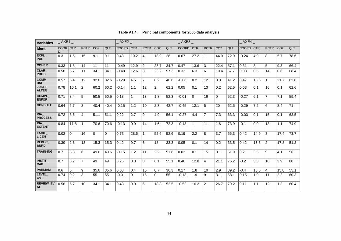
44
Table A1.4. Principal components for 2005 data analysis
Variables _ AXE1 _ _ AXE2 _ _ AXE3 _ _ AXE4 _
Ident. COORD
CTR RCTR CO2 QLT COORD CTR RCTR CO2 QLT COORD CTR RCTR CO2 QLT COORD CTR RCTR CO2 QLT
EXPL_ POL
0.3 1.5 15 9.1 9.1 0.43 10.2 4 18.9 28 0.67 27.2 1 44.9 72.9 -0.24 4.9 8 5.7 78.6
COHER 0.33 1.8 14 11 11 -0.49 12.9 2 23.7 34.7 0.47 13.6 3 22.4 57.1 0.31 8 5 9.3 66.4
CLAR_ PROC
0.58 5.7 11 34.1 34.1 -0.48 12.6 3 23.2 57.3 0.32 6.3 6 10.4 67.7 0.08 0.5 14 0.6 68.4
COMM UNI
0.57 5.4 12 32.6 32.6 -0.29 4.5 7 8.2 40.8 -0.06 0.2 12 0.3 41.2 0.47 18.6 1 21.7 62.8
JUSTIF_ ALTER
0.78 10.1 2 60.2 60.2 -0.14 1.1 12 2 62.2 0.05 0.1 13 0.2 62.5 0.03 0.1 16 0.1 62.6
COMPL_ ENFOR
0.71 8.4 5 50.5 50.5 0.13 1 13 1.8 52.3 -0.01 0 16 0 52.3 -0.27 6.1 7 7.1 59.4
CONSULT 0.64 6.7 8 40.4 40.4 -0.15 1.2 10 2.3 42.7 -0.45 12.1 5 20 62.6 -0.29 7.2 6 8.4 71
RIA_ PROCESS
0.72 8.5 4 51.1 51.1 0.22 2.7 9 4.9 56.1 -0.27 4.4 7 7.3 63.3 -0.03 0.1 15 0.1 63.5
RIA_ EXTENT
0.84 11.8 1 70.6 70.6 -0.13 0.9 14 1.6 72.3 -0.13 1 11 1.6 73.9 -0.1 0.9 13 1.1 74.9
FACIL_ LICEN
0.02 0 16 0 0 0.73 28.5 1 52.6 52.6 0.19 2.2 8 3.7 56.3 0.42 14.9 3 17.4 73.7
REDUC_ BURD
0.39 2.6 13 15.3 15.3 0.42 9.7 6 18 33.3 0.05 0.1 14 0.2 33.5 0.42 15.3 2 17.8 51.3
TRAIN-ING 0.7 8.3 6 49.6 49.6 -0.15 1.2 11 2.2 51.8 0.03 0.1 15 0.1 51.9 0.2 3.5 9 4.1 56
INSTIT_ CAP
0.7 8.2 7 49 49 0.25 3.3 8 6.1 55.1 0.46 12.8 4 21.1 76.2 -0.2 3.3 10 3.9 80
PARLIAM 0.6 6 9 35.6 35.6 0.08 0.4 15 0.7 36.3 0.17 1.8 10 2.9 39.2 -0.4 13.6 4 15.8 55.1 LEVEL_ GVT
0.74 9.2 3 55 55 -0.01 0 16 0 55 -0.18 1.9 9 3.1 58.1 0.15 1.9 11 2.2 60.3
REVIEW_EVAL
0.58 5.7 10 34.1 34.1 0.43 9.9 5 18.3 52.5 -0.52 16.2 2 26.7 79.2 0.11 1.1 12 1.3 80.4

45
Table A1.5. Principal components for 2005 linked data analysis
Variables _ AXE1 _ _ AXE2 _ _ AXE3 _ _ AXE4 _
Ident. COORD
CTR RCTR CO2 QLT COORD CTR RCTR CO2 QLT COORD CTR RCTR CO2 QLT COORD CTR RCTR CO2 QLT
EXPL_POL 0.36 3.5 10 12.8 12.8 0.71 22.4 1 50.3 63.1 -0.22 3.2 7 4.7 67.8 0.11 1 8 1.3 69.1
COHER 0.57 8.8 5 32.5 32.5 0.49 10.7 4 24 56.5 -0.33 7.4 5 10.9 67.4 -0.18 2.7 5 3.4 70.8
CLAR_PROC
0.71 13.8 3 51 51 -0.1 0.4 11 1 52 -0.28 5.2 6 7.6 59.7 -0.28 6.1 3 7.6 67.2
COMMUNI 0.58 9.2 4 34 34 -0.39 6.7 7 15.1 49.1 0.07 0.3 12 0.5 49.6 0.02 0 12 0.1 49.6
JUSTIF_ALTER
0.85 19.6 1 72.1 72.1 -0.1 0.4 12 0.9 73 -0.03 0 13 0.1 73.1 0.02 0 13 0 73.1
COMPL_ENFOR
0.04 0 13 0.2 0.2 0.06 0.2 13 0.4 0.5 0.13 1.2 9 1.8 2.3 0.81 52.2 1 65.2 67.5
CONSULT 0.31 2.6 11 9.6 9.6 -0.39 6.8 6 15.2 24.8 -0.09 0.5 11 0.8 25.6 0.6 29.2 2 36.5 62.1
RIA 0.78 16.4 2 60.6 60.6 -0.12 0.6 10 1.4 62 0.13 1.2 8 1.8 63.8 0.07 0.3 10 0.4 64.2
FACIL_LICEN
0.08 0.2 12 0.7 0.7 0.67 20 2 44.9 45.7 0.47 14.7 3 21.7 67.3 -0.08 0.5 9 0.6 68
REDUC_BURDEN
0.42 4.8 9 17.7 17.7 0.38 6.6 8 14.7 32.4 0.62 25.9 2 38.2 70.6 0.03 0.1 11 0.1 70.7
TRAINING 0.47 6 8 22.2 22.2 -0.57 14.3 3 32 54.2 -0.12 0.9 10 1.3 55.6 -0.18 2.6 6 3.2 58.8
INSTIT_CAP
0.52 7.4 7 27.3 27.3 0.44 8.5 5 19.1 46.4 -0.42 11.8 4 17.4 63.8 0.22 3.8 4 4.8 68.6
REVIEW_EVAL
0.53 7.6 6 28 28 -0.23 2.3 9 5.3 33.2 0.64 27.6 1 40.7 73.9 -0.13 1.5 7 1.8 75.7

46
Table A1.6. Principal components for 1998 data analysis
Variables _ AXE1 _ _ AXE2 _ _ AXE3 _ _ AXE4 _
Ident. COORD CTR RCTR CO2 QLT COORD CTR RCTR CO2 QLT COORD CTR RCTR CO2 QLT COORD CTR RCTR CO2 QLT
EXPL_POL
0.38 3.2 9 14.2 14.2 0.18 1.7 8 3.1 17.3 -0.23 3.9 7 5.4 22.7 0.71 42.7 1 50.7 73.4
COHER 0.11 0.3 11 1.1 1.1 0.32 5.5 4 10.3 11.4 -0.69 34 1 47 58.5 0.2 3.4 5 4.1 62.5
CLAR_PROC
0.69 10.9 6 47.6 47.6 -0.46 11.2 3 20.8 68.4 0.13 1.2 10 1.7 70.1 -0.09 0.7 9 0.8 70.9
COMMUNI 0.62 8.8 7 38.6 38.6 -0.27 3.8 6 7.1 45.7 -0.23 3.7 8 5.1 50.8 -0.44 16.2 3 19.3 70.1
JUSTIF_ALTER
0.81 14.9 2 65.1 65.1 0.14 1.1 10 2.1 67.2 -0.15 1.6 9 2.2 69.4 -0.2 3.2 6 3.8 73.2
COMPL_ENFOR
-0.04 0 13 0.2 0.2 0.75 29.8 2 55.6 55.7 0.39 11.2 3 15.5 71.2 -0.06 0.3 10 0.3 71.5
CONSULT 0.74 12.5 4 54.4 54.4 0.17 1.5 9 2.9 57.3 0.31 6.9 5 9.6 66.9 -0.01 0 13 0 66.9
RIA 0.83 15.7 1 68.5 68.5 0.23 2.7 7 5.1 73.6 -0.03 0.1 13 0.1 73.7 -0.13 1.5 7 1.8 75.5
FACIL_LICEN
0.06 0.1 12 0.3 0.3 -0.83 36.6 1 68.3 68.6 0.26 4.7 6 6.5 75.1 0.25 5.3 4 6.3 81.4
REDUC_BURDEN
0.11 0.3 10 1.2 1.2 0.29 4.4 5 8.2 9.4 0.56 22.5 2 31.2 40.6 -0.09 0.7 8 0.8 41.5
TRAINING 0.74 12.4 5 54 54 -0.11 0.7 12 1.3 55.3 -0.13 1.2 11 1.6 57 -0.03 0.1 12 0.1 57.1
INSTIT_CAP
0.56 7.2 8 31.7 31.7 -0.04 0.1 13 0.2 31.8 0.35 8.8 4 12.2 44 0.55 25.7 2 30.5 74.5
REVIEW_EVAL
0.78 13.8 3 60.4 60.4 0.13 1 11 1.8 62.2 -0.05 0.2 12 0.2 62.4 0.04 0.1 11 0.2 62.6

47
Description of external indicators
Doing Business Indicator (DBI)
The Doing Business database indicates the regulatory costs of business. Economies are ranked on
their ease of doing business, from 1 to 175, with first place being the best. In 2008, the aggregate indicator
on “Ease of Doing Business” is an average of the country's percentile rankings on the following ten topics:
1. Starting a business: identifies bureaucratic and legal hurdles an entrepreneur must overcome to
incorporate and register a new firm.
2. Dealing with licences: tracks the procedures, time, and costs to build a warehouse, including
obtaining necessary licences and permits, completing required notifications and inspections, and
obtaining utility connections.
3. Employing workers: measures the flexibility of labour regulations.
4. Registering property: examines the steps, time, and cost involved in registering property
5. Getting credit: explores two sets of issues, credit information registries and the effectiveness of
collateral and bankruptcy laws in facilitating lending.
6. Protecting investors: measures the strength of minority shareholder protections against misuse of
corporate assets by directors for their personal gain.
7. Paying taxes: addresses the taxes and mandatory contributions that a medium-size company must
pay or withhold in a given year, as well as measures of administrative burden in paying taxes.
8. Trading across borders: looks at the procedural requirements for exporting and importing a
standardised cargo of goods.
9. Enforcing contracts: looks at the efficiency of contract enforcement by following the evolution of
a sale of goods dispute and tracking the time, cost, and number of procedures involved from the
moment the plaintiff files the lawsuit until actual payment.
10. Closing a business: identifies weaknesses in existing bankruptcy law and the main procedural and
administrative bottlenecks in the bankruptcy process.
The methodology has been expanded and adapted over time. Therefore, some of the single scores are
not always directly comparable from year to year.

48
Global Competitiveness Index (GCI)
The variables are organised into 12 pillars in 2008, with each component representing an area
considered to be an important determinant of competitiveness:
Basic requirements
1. Institutions. This includes public and private institutions. Questions are related to property rights,
diversion of public funds, wastefulness of government spending, organised crime, strength of
auditing and accounting standards, among other issues.
2. Infrastructure. Deals with overall infrastructure quality, telephone lines, among others.
3. Macroeconomic stability. Questions are related to government surplus and deficit, inflation,
among others.
4. Health and primary education. Examines life expectancy, primary enrolment rates among other
issues.
Efficiency enhancers
5. Higher education and training. Deals with secondary and tertiary enrolment rates, quality of the
educational system, among others.
6. Goods market efficiency. Questions are related to the extent of staff training, extent and effect of
taxation, prevalence of trade barriers, exports, hiring and firing practices, pay and productivity,
financial market sophistication, soundness of banks, FDI and technology transfer.
7. Labour market efficiency.
8. Financial market sophistication.
9. Technological readiness. Measures internet users.
10. Market site.
Innovation and sophistication factors
11. Business sophistication. Questions are related to local supplier quality and quantity, extent of
marketing, nature of competitive advantage.
12. Innovation. Examine quality of scientific research institutions, company spending on R&D,
availability of scientist and engineers, utility patents.
The lower the index, the better the position of a given country around a given indicators. Many of the
published sources include a mix of external data, sometimes including OECD sources for OECD countries.
A detailed set of data tables presents the underlying data used for the main composite indicator. The
methodology again may have changed slightly from year to year, with constant adaptations and
improvements.

49
Worldwide Governance Indicators (WGI)
The indicator is based on sub-indicators that are measured in units ranging from -2.5 to 2.5, with
higher values corresponding to better governance outcomes:
Government effectiveness: The quality of public services, the quality of the civil service and the
degree of its independence from political pressures, the quality of policy formulation and
implementation, and the credibility of the government’s commitment to such policies.
Regulatory quality: The ability of the government to formulate and implement sound policies and
regulations promoting private sector development.
Rule of law: The extent to which agents have confidence in and abide by the rules of society, and
in particular the quality of contract enforcement, the police, and the courts, as well as the
likelihood of crime and violence.
Control of corruption: The extent to which public power is exercised for private gain, including
both petty and grand forms of corruption, as well as “capture” of the state by elites and private
interests.
Voice and accountability: The extent to which country’s citizens are able to participate in
selecting their government, as well as freedom of expression, freedom of association, and a free
media.
Political stability and absence of violence: The perceptions of the likelihood that the government
will be destabilised or overthrown by unconstitutional or violent means, including domestic
violence and terrorism.
Product Market Regulation (PMR) indicator
The OECD indicators of Product Market Regulation (PMR) provide a comprehensive and
internationally comparable set of indicators that measure the degree to which policies promote or inhibit
competition in areas of the product market where competition is thought to be viable. They measure the
regulatory and market environments in OECD countries in 1998 and 2003 and are consistent across time.
The PMR indicators summarise a large set of formal rules and regulations that have a bearing on
competition in OECD countries. In particular:
State control: Assess the impact of public ownership (through the scope and size of public
enterprise sector, and the direct control over business enterprises) and the involvement in
business operation (through price controls and use of command and control regulations).
Barriers to entrepreneurship: Licences, permits system, communication and simplification of
rules and procedures, administrative burdens for corporations, for sole proprietor firms and for
specific sectors, antitrust exemptions and legal barriers measure the regulatory and administrative
opacity as well as the administrative burdens on start-ups.
Barriers to trade and investment: Examine foreign ownership barriers, discriminatory
procedures, tariffs and other regulatory barriers.
The scale goes from least restrictive (0) to most restrictive (6).

50
The OECD Regulatory Management System indicator
The Principal Component Analysis allows obtaining some weights for the different categories
measuring regulatory quality. The PCA aggregates the 16 (or 13) sub-indicators that are slightly
interrelated and correlated. Therefore it reduces the number of sub-indicators, as well as the correlation
among the different sub-indicators. These newly created variables are called the principal components. The
advantages of using PCA for the construction of a composite indicator are:
the construction of the composite no longer depends upon the number of dimensions of the
dataset but instead upon the broader characteristics of the data itself;
redundant information is reduced: if for instance two different variables both having a weight of
1 measure the exact same information, these two variables will not receive a total weight of 2
together but instead be weighed together with a weight of 1 by an indicator based on PCA;
the underlying principle is to account for the highest possible variation in the variables using the
smallest possible number of components.
The methodology used is similar to the one described and recommended in the European Commission
Paper “Tools for Composite Indicators Building”.1 The construction of the composite indicator was also
based on the methodology of the “Handbook on constructing composite indicators”.2
The first principal components explain a large share of the total variance within the dataset
(approximately a third to close to 40% in the current sample). The weights used for constructing the
aggregate indicator are based on the first four principal components. The first two of these components are
presented in detail in the first section of the note. Characteristics of the components are presented below.
The composite indicator is constructed by using the squared factor loadings, i.e. the squared
coordinates for each of the variables, measuring regulatory quality. Each variable has a specific factor
loading for each component, which is calculated as part of the PCA aggregation procedure. The reason for
using squared factor loadings is that they represent the proportion of a components variance (i.e.
information), which is explained by a specific variable. This procedure permits to retain four factor
loadings for each variable, which are used as basic weights. Hence each weight corresponds to the degree
that a variable can explain of the information available in the four components that allow for meaningful
interpretation.
Final weights for each of the variables measuring the different aspects of high quality regulation are
obtained by summing up the four basic weights. Each of the four basic weights for a variable corresponds
to the variation of a specific principal component that can be explained by that variable. Therefore the final
weight for a variable can be interpreted as the part of the overall meaningful variance, which can be
explained by that variable. The preceding procedure gives 16 final weights for the different categories
measuring high quality regulation. In order to obtain the final scores for an individual country, each of
these 16 weights is multiplied with the country's corresponding score for the category measured by an
individual weight and then the weighted scores are added for each country. The sensitivity of the scores
obtained can be tested with random weights simulation techniques, called Monte Carlo simulation
techniques. This offers a range of uncertainty.
1. “Tools for Composite Indicators Building” by Michela Nardo, Michaela Saisana, Andrea Saltelli and
Stefano Tarantolo published by the European Commission 2005 Reference: EUR 21682EN.
2. “Handbook on constructing composite indicators: Methodology and User Guide” by Michela Nardo,
Michaela Saisana, Andrea Saltelli and Stefano Tarantola (EC/JRC) and, Anders Hoffman and Enrico
Giovannini (OECD).

51
Table A1.7. Correlations of RMS with World Bank Doing Business Indicators
RMS1 _05
RMS2_05
IND_AV05
IND_AG05
RMS1_05lk
RMS2_05lk
IND_AV05lk
IND_AG05lk
DB05 -0.43** 0.28 -0.31 -0.29 -0.38** 0.52*** -0.13 -0.10 Ease of doing business rank in 2005 0.02 0.14 0.10 0.13 0.05 0.01 0.52 0.61
29 29 29 29 27 27 27 27
DB05_SB -0.30 0.25 -0.18 -0.15 -0.25 0.51*** 0.01 0.03 DB05 : Starting a business rank 0.11 0.18 0.35 0.42 0.21 0.01 0.97 0.87
29 29 29 29 27 27 27 27
DB05_SBP -0.24 0.41** -0.11 -0.09 -0.15 0.66*** 0.14 0.17 DB05 : Starting a business (Number of procedures) 0.20 0.03 0.58 0.63 0.45 0.00 0.49 0.41
29 29 29 29 27 27 27 27
DB05_SBT -0.35*** 0.25 -0.25 -0.23 -0.34* 0.35* -0.14 -0.11 DB05 : Starting a business (Time in days) 0.06 0.19 0.19 0.23 0.09 0.08 0.50 0.58
29 29 29 29 27 27 27 27
DB05_DL -0.21 0.04 -0.14 -0.14 -0.21 0.30 -0.07 -0.04 DB05 : Dealing with licences rank 0.28 0.85 0.46 0.47 0.30 0.13 0.71 0.85
29 29 29 29 27 27 27 27
DB05_DLP 0.02 -0.07 0.01 0.01 0.00 0.09 0.01 0.03 DB05 : Dealing with licences (Number of procedures) 0.92 0.72 0.94 0.97 0.98 0.67 0.97 0.89
29 29 29 29 27 27 27 27
DB05_DLT -0.44** 0.16 -0.31 -0.31 -0.46** 0.39** -0.26 -0.22 DB05 : Dealing with licences (Time in days) 0.02 0.40 0.10 0.11 0.01 0.04 0.18 0.28
29 29 29 29 27 27 27 27
DB05_EW -0.40** 0.24 -0.35* -0.32* -0.27 0.34* -0.08 -0.06 DB05 : Employing workers rank 0.03 0.21 0.07 0.09 0.18 0.08 0.68 0.75
29 29 29 29 27 27 27 27
DB05_RP -0.25 0.41** -0.13 -0.12 -0.22 0.35* 0.01 0.02 DB05 : Registering property rank 0.19 0.03 0.49 0.52 0.27 0.07 0.96 0.92
29 29 29 29 27 27 27 27
DB05_CB -0.15 0.06 -0.07 -0.07 -0.15 0.30 -0.03 -0.03 DB05 : Closing a business rank 0.44 0.76 0.72 0.73 0.46 0.13 0.87 0.88
29 29 29 29 27 27 27 27

52
Table A1.8. Correlations of OECD RMS with WEF Global Competitiveness Indicators (2005)
RMS1_05
RMS2_05
IND_AV 05
IND_AG05
RMS1_ 05lk
RMS2_ 05lk
IND_AV05lk
IND_AG05lk
GCI05 -0.21 0.17 -0.13 -0.11 -0.21 0.32 -0.04 -0.02
Global competitiveness index rank in 2005 0.27 0.37 0.49 0.56 0.30 0.11 0.83 0.93
30 30 30 30 27 27 27 27
RGCI05_I -0.14 0.24 -0.04 -0.02 -0.14 0.53*** 0.08 0.10
Rank of GCI05_Institutions 0.47 0.21 0.85 0.91 0.49 0.00 0.70 0.61
30 30 30 30 27 27 27 27
RGCI05_IB -0.06 0.21 0.06 0.05 -0.06 0.42** 0.12 0.12
Rank of GCI05_Inst_Burden of government regulation 0.77 0.27 0.77 0.78 0.78 0.03 0.57 0.53
30 30 30 30 27 27 27 27
RGCI05_M -0.37** 0.25 -0.26 -0.23 -0.37* 0.44** -0.15 -0.13
Rank of GCI05_Markets Efficiency 0.04 0.19 0.17 0.22 0.06 0.02 0.45 0.52
30 30 30 30 27 27 27 27
RGCI05_ME 0.06 0.13 0.14 0.14 0.06 0.41** 0.22 0.24
Rank of GCI05_Efficiency of Legal Framework 0.77 0.48 0.46 0.47 0.78 0.03 0.27 0.22
30 30 30 30 27 27 27 27

53
Table A1.9. Correlations of OECD RMS with World Bank Governance Indicators (2005)
RMS1_05
RMS2_05
IND_AV 05
IND_AG05
RMS1_ 05lk
RMS2_ 05lk
IND_AV05lk
IND_AG05lk
WGI05_TO 0.03 -0.27 -0.09 -0.10 0.05 -0.62*** -0.19 -0.21 World governance index in 2005 0.87 0.15 0.65 0.60 0.80 0.00 0.35 0.29
30 30 30 30 27 27 27 27
WGI05_AV 0.05 -0.20 -0.05 -0.06 0.09 -0.57*** -0.13 -0.15 World governance (average) index in 2005 0.78 0.30 0.78 0.73 0.66 0.00 0.51 0.45
30 30 30 30 27 27 27 27
WGI_GE05 0.05 -0.18 -0.04 -0.05 0.07 -0.57*** -0.13 -0.15 WGI_Government Effectiveness 05 0.79 0.33 0.84 0.78 0.73 0.00 0.53 0.47
30 30 30 30 27 27 27 27
WGI_RQ05 0.10 -0.22 -0.03 -0.05 0.16 -0.52*** -0.05 -0.07 WGI_Regulatory Quality 05 0.59 0.24 0.86 0.79 0.43 0.01 0.82 0.75
30 30 30 30 27 27 27 27
WGI_RL05 0.07 -0.20 -0.02 -0.03 0.09 -0.58*** -0.13 -0.15 WGI_Rule of Law 05 0.72 0.30 0.94 0.88 0.66 0.00 0.52 0.44
30 30 30 30 27 27 27 27
WGI_CC05 0.12 -0.29 0.01 -0.01 0.07 -0.60*** -0.16 -0.18 WGI_Control of Corruption 05 0.53 0.12 0.98 0.97 0.72 0.00 0.42 0.36
30 30 30 30 27 27 27 27

54
Table A1.10. Correlations of OECD RMS with World Bank Governance Indicators (1998)
RMS1_98 RMS2_98 IND_AV98 IND_AG98
WGI98_TO 0.27 0.22 -0.01 -0.01 WGI98_TOTAL 0.17 0.26 0.98 0.94 27 27 27 27
WGI98_AV 0.30 0.20 0.05 0.04 WGI98_AVERAGE 0.13 0.31 0.81 0.85 27 27 27 27
WGI_GE98 0.16 0.20 -0.04 -0.04 WGI_Government Effectiveness 98 0.42 0.32 0.84 0.84 27 27 27 27
WGI_RQ98 0.35* 0.17 0.13 0.12 WGI_Regulatory Quality 98 0.07 0.39 0.53 0.56 27 27 27 27
WGI_RL98 0.27 0.21 0.00 -0.01 WGI_Rule of Law 98 0.18 0.28 0.98 0.96 27 27 27 27
WGI_CC98 0.23 0.15 -0.02 -0.03 WGI_Control of Corruption 98 0.24 0.45 0.91 0.88 27 27 27 27

55
Figure A1.1 Trends in Product Market Regulation and Administrative Simplification Policies
Correlation between trends in REGREF 1998-2005 and RMS2_05 in 2005
RMS2_05
6.005.004.003.002.001.00
SLO
PREG
0.10
0.00
-0.10
-0.20
-0.30
-0.40
-0.50
USA
UK
SWE
PRT
NZL
NOR
NLD
JPN
ITA
IRL
GRE
FRA
FIN
ESPDNK
DEU
CHE
CAN
BELAUT
AUS
R Sq Linear = 0.273
Correlation between trends in REGREF 1998-2005 and RMS2_05 linked data in 2005
RMS2_05L
8.007.006.005.004.003.002.00
SLO
PREG
0.10
0.00
-0.10
-0.20
-0.30
-0.40
-0.50
USA
UK
SWE
PRT
NZL
NOR
NLD
JPN
ITA
IRLGRE FRA
FIN
ESPDNK
DEU
CHE
CAN
BELAUT
AUS
R Sq Linear = 0.376

56
Correlation between trends in Product Market Regulation 1998-2003 and RMS2_05 linked data in 2005
RMS2_05
6.005.004.003.002.001.00
SLO
PPM
R
0.00
-0.05
-0.10
-0.15
-0.20
-0.25
-0.30
USAUK
TUR
SWE PRT
POL
NZL
NOR NLD
MEX
KOR
JPN
ITA
IRL
ICE
HUN
GRE
FRAFIN
ESP
DNK
DEU
CZE
CHE
CAN
BEL
AUT
AUS
R Sq Linear = 0.026
Correlation between trends in Product Market Regulation 1998-2003 and RMS2_05 linked data in 2005
RMS2_05L
8.006.004.002.00
SLO
PPM
R
0.00
-0.05
-0.10
-0.15
-0.20
-0.25
-0.30
USAUK
TUR
SWE PRT
NZL
NOR
NLD
MEX
KOR
JPN
ITA
IRL
ICE
HUN
GRE
FRA
FINESP
DNK
DEU
CZE
CHE
CAN
BEL
AUT
AUS
R Sq Linear = 0.08

57
Correlation between trends in REGREF 1998-2005 and RMS2_98 in 1998
RMS2_98
6.004.002.000.00
SLO
PREG
0.10
0.00
-0.10
-0.20
-0.30
-0.40
-0.50
USA
UK
SWE
PRT
NZL
NOR
NLD
JPN
ITA
IRLGRE
FRA
FIN
ESPDNK
DEU
CHE
CAN
BELAUT
AUS
R Sq Linear = 0.124
Correlation between trends in Product Market Regulation 1998-2005 and RMS2_98 in 1998
RMS2_98
6.004.002.000.00
SLO
PPM
R
0.00
-0.05
-0.10
-0.15
-0.20
-0.25
-0.30
USA
UK
TUR
SWEPRT
NZL
NOR
NLD
MEX
KOR
JPN
ITA
IRL
ICE
HUN
GRE
FRAFIN
ESP
DNK
DEU
CZE
CHE
CAN
BEL
AUT
AUS
R Sq Linear = 0.085

58
Table A1.11. Fixed effects regressions with RMS1 indicator
Interpolated indicator
Total employment,
business sector
Total employment
Gdp, business
sector
Labour productivity
business sector
Total employment,
Business sector
Total employment
Gdp, business
sector
Labour productivity
business sector
RMS
1 631252.2** 240730.9*** 1.32e+10 0.023677** 505542.4* 239058.6*** 1.31e+10 0.0239024***
(431638.8) (69421.85) (1.09e+10) (0.0114452) (279393.1) (61215.25) (1.04e+10) (0.0050503) Constant 1.51e+07*** 1.54e+07*** 6.66e+11*** 10.50025 1.62e+07*** 1.53e+07*** 6.68e+11*** 10.51155*** (2300224) (369952.4) (5.78e+10) (0.0621939) (1488899) (326219) (5.56e+10) (0.271418) Fixed Effects Yes Yes Yes Yes Yes Yes Yes Yes RSE
2 Yes Yes Yes No Yes Yes Yes No
Heteroskedasticity Test
0.0002 0.0000 0.0000 0.6385 0.0000 0.0000 0.0000 0.8642
Observations 42
42 42 42 168 168 168 168
R-square 0.0550
0.0656 0.0102 0.1763 0.0331 0.0568 0.0107 0.1330
1 RMS1: 1998 and 2005 (T=2); RMS1 links regulatory institutions and tools;
2 RSE: Robust standard errors, in parentheses where indicated; * significant at 10%; **
significant at 5%; *** significant at 1%

59
Table A1.12. Fixed effects regressions with RMS simple average indicator
Interpolated indicator
Total employment,
business sector
Total employment
GDP, business
sector
Labour productivity
business sector
Total employment,
business sector
Total employment
GDP, business
sector
Labour productivity
business sector
RMS_av
1 1027860* 401034.9*** 3.64e+10*** 0.0311715*** 801667** 370628.2*** 3.55e+10*** 0.0315929***
(593474.2) (125159.4) (1.26e+10) (0.0108126) (378128.5) (110182.3) (1.21e+10) (0.0048719) Constant 1.36e+07*** 1.48e+07*** 5.64e+11*** 10.47919*** 1.51e+07*** 1.48e+07*** 5.70e+11*** 10.4897*** (2803318) (591199.4) (5.95e+10) (0.052302) (1786117) (520453.9) (5.70e+10) (0.0232519) Fixed Effects Yes Yes Yes Yes Yes Yes Yes Yes RSE
2 Yes Yes Yes No Yes Yes Yes no
Heteroskedasticity Test
0.0014 0.0000 0.0000 0.7025 0.0000 0.0000 0.0000 0.3826
Observations 42 42 42 42 168 168 168 168
R-square 0.1400 0.1748 0.0749 0.2936 0.0802 0.1314 0.0756 0.2236 1
RMS_av: 1998 and 2005 (T=2), 2
RSE: Robust standard errors, in parentheses where indicated
* significant at 10%; ** significant at 5%; *** significant at 1%

60
Table A1.13. Fixed Effects regressions with RMS weighted aggregated indicator
Interpolated indicator
Total Employment,
Business Sector
Total Employment
GDP, Business
Sector
Labour Productivity
Business sector
Total Employment,
Business Sector
Total Employment
GDP, Business
Sector
Labour Productivity
Business sector
RMS_ag
1 78542.31** 33006.02*** 3.27e+09** 0.0023343*** 62841.25** 30160.38*** 3.18e+09*** 0.0023611***
(40906.13) (10326.82) (1.43e+09) (0.0007788) (27040.57) (8970.336) (1.36e+09) (0.0003526) Constant 1.47e+07*** 1.51e+07*** 5.81e+11*** 10.51623*** 1.59e+07*** 1.51e+07*** 5.88e+11*** 10.52746*** (1931120) (487514.4) (6.73e+10) (0.384168) (1276547) (423476.8) (6.41e+10) (0.0169711) Fixed Effects Yes Yes Yes Yes Yes Yes Yes Yes RSE
2 Yes Yes Yes No Yes Yes Yes No
Heteroskedasticity Test
0.0053 0.0000 0.0000 0.5822 0.0000 0.0000 0.0000 0.3009
Observations 42 42 42 42 168 168 168 168 R-square 0.1539 0.2229 0.1141 0.3099 0.927 0.1637 0.1144 0.2349
1RMS_ag: 1998-2005 (T=7), 2 RSE: Robust standard errors, in parentheses where indicated * significant at 10%; ** significant at 5%; *** significant at 1%

61
Table A1.14. Random Effects regressions with interpolated RMS 1 indicator
Total employment, business sector
Total employment
GDP, business sector Labour productivity, business sector
Interpolated RMS
1 517044.7**
240683.9***
1.39e+10*
0.0236398***
(225254) (80486.91) (1.04e+10) (0.0049524) Constant 1.61e+07** 1.53e+07** 6.64e+11** 10.51295*** (6934662) (6092609) (3.12e+11) (0.059611) Random Effects Test 0.5270 0.7160 0.0409 0.7907 Observations 168 168 168 168 R-square 0.0403 0.0335 0.0736 0.0213
1RMS interpolated between 1998 and 2005 to yield T=7; RMS1 links regulatory institutional and tools; * significant at 10%; ** significant at 5%; *** significant at 1%.

62
Table A1.15. Random effects regressions with interpolated RMS av indicator
Total employment, business sector
Total employment
GDP, business sector
Labour productivity, business sector
Interpolated RMS_av
1 807375.6*** 371392.2*** 3.59e+10*** 0.0315704***
(224394.3) (78771.97) (1.03e+10 ) (0.0048404) Constant 1.51e+07** 1.48e+07** 5.68e+11** 10.4898*** (6909027) (6086279) (3.11e+11) (0.0582573) Random Effects Test 0.6250 0.8366 Not asymptotic 0.9675 Observations 168 168 168 168 R-square 0.0328 0.0263 0.0566 0.0198
1 RMS_av interpolated between 1998 and 2005 to yield T=7
* significant at 10%; ** significant at 5%; *** significant at 1%

63
Table A1.16 Random effects regressions with interpolated RMS ag indicator
Total employment, business sector
Total employment
GDP, business sector Labour productivity, business sector
Total Employment
Total Employment, Business Sector
GDP, Business Sector
Labour Productivity Business sector
Interpolated RMS_ag
1 63117.77*** 30195.89*** 3.20e+09*** 0.0023614***
(16250.48) (5634.643) (7.33e+08) (0.000351) Constant 1.59e+07** 1.51e+07** 5.87e+11** 10.52745*** (6889079) (6095208) (3.11e+11) (0.0561786) Random Effects Test 0.7394 0.9018 asymptotic 0.9923 Observations 168 168 168 168
R-square 0.0227 0.0177 0.0396 0.0168 1 RMS_ag interpolated between 1998 and 2005 to yield T=7
* significant at 10%; ** significant at 5%; *** significant at 1%.

64
Table A1.17. Fixed effects regressions with PMR indicator
Interpolated indicator
Total employment
business sector
Total employment
GDP, business
sector
Labour productivity business
sector
Total employment,
business sector
Total employment
GDP, business
sector
Labour productivity business
sector
Constant 8479435*** 1.06E+07*** 4.56E+11*** 10.833*** 8449122*** 1.07E+07*** 4.63E+11*** 10.859*** (444341.8) (676065.6) (4.14E+10) (0.029) (234972.2) (423287.4) (2.39E+10) (0.020) PMR -634986.2* -1494733* -9.84E+10 -0.115*** -636816.8*** -1580271*** -
1.00E+11*** -0.119***
(317619.4) (611511.1) (3.84E+10) (0.027) (202706.7) (392958.6) (2.22E+10) (0.017) Fixed Effects Yes Yes Yes Yes Yes Yes Yes Yes RSE
2 Yes Yes Yes Yes Yes Yes Yes Yes
Heteroskedasticity Test
0.0006 0.000 0.000 0.0010 0.000 0.000 0.000 0.000
Observations 42 42 42 42 126 126 126 126 R-square 0.10 0.10 0.10 0.97 0.10 0.10 0.10 0.98 1RSE: Robust standard errors in parentheses; 4 PMR: 1998 and 2003 (T=2).
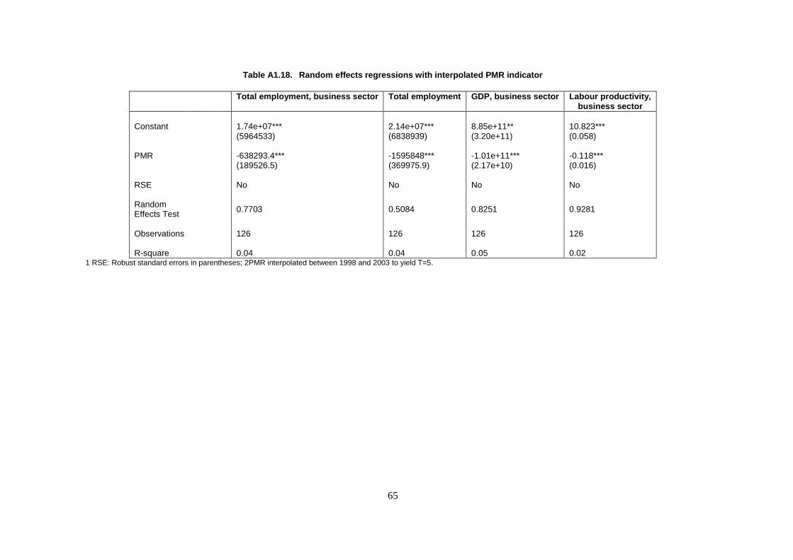
65
Table A1.18. Random effects regressions with interpolated PMR indicator
Total employment, business sector
Total employment
GDP, business sector Labour productivity, business sector
Constant 1.74e+07*** 2.14e+07*** 8.85e+11** 10.823*** (5964533) (6838939) (3.20e+11) (0.058) PMR -638293.4*** -1595848*** -1.01e+11*** -0.118*** (189526.5) (369975.9) (2.17e+10) (0.016) RSE No No No No Random Effects Test
0.7703 0.5084 0.8251 0.9281
Observations 126 126 126 126 R-square 0.04 0.04 0.05 0.02
1 RSE: Robust standard errors in parentheses; 2PMR interpolated between 1998 and 2003 to yield T=5.

66
NOTE: FIXED VERSUS RANDOM EFFECTS
Consider the following model with a single explanatory variable:3
itiitit uaXy ,
where the error contains a time constant component, ai.
Fixed Effects effectively removes the ai prior to estimation. Fixed Effects consists in subtracting time
averages from each variable, and performing least squares on the transformed model:
iitiitiit uuxxyy )( .
Note that in addition to ai, any time constant variables are also eliminated in this transformation.
Random Effects takes an alternative approach. It assumes that any unobserved individual
heterogeneity only induces serial correlation in the error, and not between the errors and explanatory
variables. Random Effects assumes:
0,cov iit ax for all time periods, t.
Under this assumption, the aggregate error may be written as:
itiit uav
And the model becomes ititit vXy
The errors are now serially correlated across t:
22
2
,au
u
isit vvcorr
for t different from s.
Estimation consists in making the GLS transformation:
iitiitiit vvxxyy )(
Where 2
1
22
2
1
au
u
T
It is worth noting that both Pooled OLS and Fixed Effects are limiting cases of Random Effects: when
l = 0, Random Effects is Pooled OLS, while when l = 1, Random Effects is Fixed Effects.
3. This may be easily generalised to the case of multiple regressors.