Embed Size (px)
Citation preview

Systems of Index Numbers for International Price Comparisons
Based on the Stochastic Approach
Gholamreza HajargashtGholamreza HajargashtD.S. Prasada RaoD.S. Prasada Rao
Centre for Efficiency and Productivity AnalysisCentre for Efficiency and Productivity AnalysisSchool of EconomicsSchool of Economics
University of QueenslandUniversity of QueenslandBrisbane, Australia Brisbane, Australia

Motivation – multilateral comparisons of prices
Standard formulae and the new index formula
Stochastic approach to index numbers
Derivation of index numbers using stochastic approach
Empirical application – OECD data
Concluding remarks
OutlineOutline
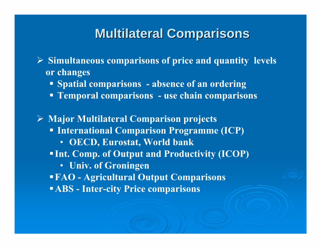
Multilateral ComparisonsMultilateral Comparisons
Simultaneous comparisons of price and quantity levels or changes
Spatial comparisons - absence of an orderingTemporal comparisons - use chain comparisons
Major Multilateral Comparison projectsInternational Comparison Programme (ICP)• OECD, Eurostat, World bank
Int. Comp. of Output and Productivity (ICOP)• Univ. of Groningen
FAO - Agricultural Output ComparisonsABS - Inter-city Price comparisons

Role of Multilateral ComparisonsRole of Multilateral Comparisons
Purchasing Power Parities • Cross-country comparisons of price levels• Real GDP and Expenditure components
ICP, OECD and EurostatPenn World Tables (PWT) - Heston and
SummersReal income comparisons, HDI etc.Global inequalityGrowth and Productivity
• Catch-up and Convergence studiesGlobal poverty - World Bank
Output and Input index numbers• Productivity comparisons (TFP, DEA, SFA)

Index Number ProblemIndex Number ProblemPrice and Quantity Data
Commodities
Countries 1 2 3 i N
1 p11 q11 p21 q21 p31 q31 pi1 qi1 pN1 qN1
2 p12 q12 p22 q22 p32 q32 pi2 qi2 pN2 qN2
3 p13 q13 p23 q23 p33 q33 pi3 qi3 pN3 qN3
.
j
.
pij qij
M p1M q1M p2M q2M p3M q3M piM qiM pNM qNM
⎥⎥⎥⎥⎥⎥
⎦
⎤
⎢⎢⎢⎢⎢⎢
⎣
⎡
=
MM1M
M22221
M11211
MxM
I...I..........
I..III..II
I
•Transitivity: Ijk = Ijl x Ilk- a consistency requirement
•Base invariance - country symmetry

There exist numbers PPP1, PPP2, …., PPPM such that any index Ijk can be expressed as:
These PPP’s can be determined only upto a factor of proportionality.
Once the PPPs are given, it is possible to define “international average Prices” for each of the commodities: P1, P2, …., PN
Implications of TransitivityImplications of Transitivity
kjk
j
PPPIPPP
=

NotationNotation
We have We have MM countries and countries and NN commoditiescommodities
observed price of the observed price of the ithith commodity in the commodity in the jthjth countrycountry
quantity of the quantity of the ithith commodity in the commodity in the jthjth country country
purchasing power parity of purchasing power parity of jthjth countrycountry
Average price for Average price for ithith commoditycommodity
sharesshares
ijp
ijq
iP
1
ij ijij N
ij iji
p qw
p q=
=
∑
*
1
ijij M
ijj
ww
w=
=
∑
jPPP

Commonly used methods like Laspeyres, Paasche, Fisher and Tornqvist methods are for bilateral comparisons – not transitive.
Geary-Khamis method – Geary (1958), Khamis (1970)
Elteto-Koves-Szulc (EKS) method – 1968
EKS method constructs transitive indexes from bilateral Fisher indexes
Weighted EKS index – Rao (2001)
Index number methods for international Index number methods for international comparisonscomparisons

Variants of Geary-Khamis method – Ikle (1972), Rao (1990)
Methods based on stochastic approach:
Country-product-dummy (CPD) method –Summers (1973)
Weighted CPD method – Rao (1995)
Generating indexes using Weighted CPD method – Rao (2005), Diewert (2005)
Using CPD to compute standard errors – Rao (2004), Deaton (2005)
Index number methods Index number methods -- continuedcontinued
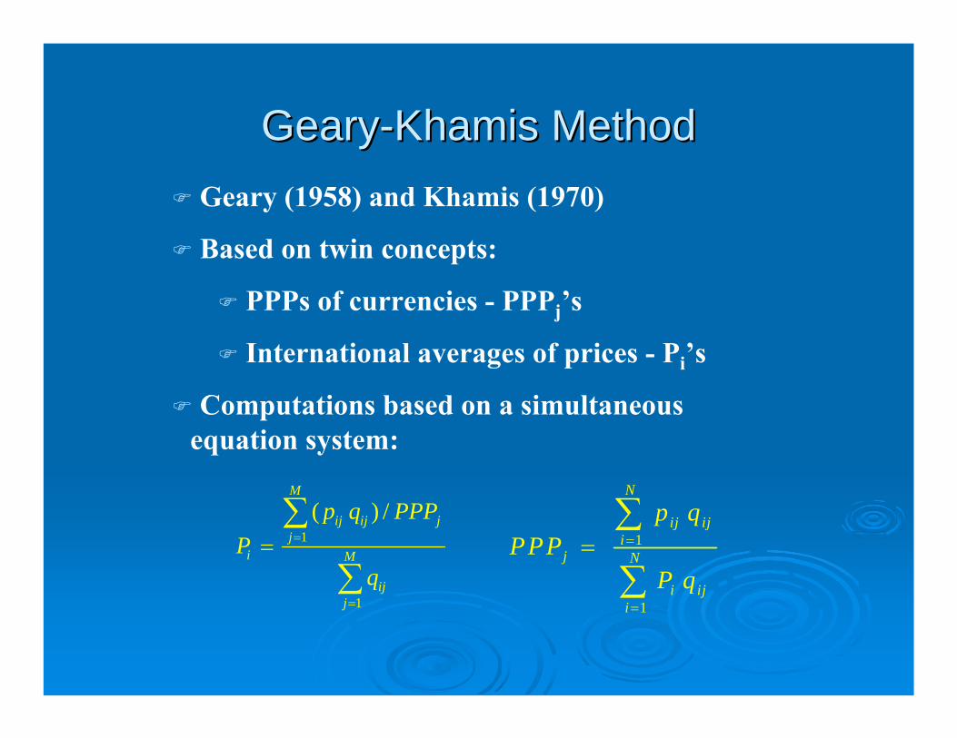
GearyGeary--Khamis MethodKhamis MethodGeary (1958) and Khamis (1970)
Based on twin concepts:
PPPs of currencies - PPPj’s
International averages of prices - Pi’s
Computations based on a simultaneous equation system:
1
1
( ) /M
ij ij jj
i M
ijj
p q PPPP
q
=
=
=∑
∑1
1
N
ij iji
j N
i iji
p qPPP
P q
=
=
=∑
∑

Rao and Rao and IkleIkle variantsvariants
Rao Index Geometric Mean Rao Index Geometric Mean
IkleIkle Index Harmonic Mean Index Harmonic Mean
1
ijwNij
jii
pPPP
P=
⎛ ⎞= ⎜ ⎟
⎝ ⎠∏
*
1
ijwMij
ijj
pP
PPP=
⎛ ⎞= ⎜ ⎟⎜ ⎟
⎝ ⎠∏
1
1 Ni
ijj iji
P wPPP P=
⎛ ⎞= ⎜ ⎟⎜ ⎟
⎝ ⎠∑
*
1
1 Mj
iji ijj
PPPw
P p=
⎛ ⎞= ⎜ ⎟⎜ ⎟
⎝ ⎠∑

The New IndexThe New Index
Why not an arithmetic meanWhy not an arithmetic mean
1
Nij
j ijii
pPPP w
P=
⎛ ⎞= ⎜ ⎟
⎝ ⎠∑
*
1
Mij
i ijjj
pP w
PPP==∑
Comments:
• For all these methods it is necessary to establish the existence of solutions for the simultaneous equations.
• Existence of Rao and Ikle indexes was established in earlier papers.
• Existence of the new index is considered in this paper.

Relationship between the indices and Relationship between the indices and stochastic approachstochastic approach
The stochastic approach to multilateral indexes is based on the CPD model – discussed below.
The indexes described above are all based on the Geary-Khamis framework which has no stochastic framework.
Rao (2005) has shown that the Rao (1990) variant of the Geary-Khamis method can be derived using the CPD model.
Rest of the presentation focuses on the connection between the CPD model and the indexes described above.

The Law of One PriceThe Law of One PriceFollowing Summers (1973), Rao (2005) and Following Summers (1973), Rao (2005) and Diewert (2005) we considerDiewert (2005) we consider
price of price of ii--thth commodity in commodity in jj--thth countrycountry purchasing power paritypurchasing power parity
ij i j ijp P PPP u=
World price of i-th commodity •random disturbance
The CPD model may be considered as a “hedonic regression model”where the only characteristics considered are the “country” and the “commodity”.

CPD ModelCPD ModelRao (2005) has shown that applying a weighted least Rao (2005) has shown that applying a weighted least square to the following equation results in Raosquare to the following equation results in Rao’’s s SystemSystem
where where are treated as parameters are treated as parameters The same result is obtained if we assume a logThe same result is obtained if we assume a log--normal normal distribution for distribution for uuijij and use a weighted maximum and use a weighted maximum likelihood estimation approach which is the same as the likelihood estimation approach which is the same as the weighted least squares estimator.weighted least squares estimator.
ln ln lnij i j ijp P PPP ε= + +
ln and lni jP PPP

Stochastic Approach to New IndexStochastic Approach to New Index
AgainAgain
This time assume This time assume
ij i j ijp PPPP u=
~ ( , )iju Gamma r r

Maximum LikelihoodMaximum Likelihood
It can be shown It can be shown
Taking logs we obtain Taking logs we obtain
1
( )( )
ij
i j
pr rr
PPPPijij r r
i j
prf p er P PPP
− −
=Γ
ln ln ( ) ( 1) ln ln ln ijij ij i j
i j
pLnL r r r r p r P r PPP r
PPPP= − Γ + − − − −

Weights and MWeights and M--EstimationEstimation
Define a weighted likelihood asDefine a weighted likelihood as
Then we haveThen we have
1 1 1 1 1 1ln ( 1) ln ln ln
n n n n n n
ij ij ij i ij ji j i j i j
WL r w p r w P r w PPP= = = = = =
∝ − − − −∑∑ ∑∑ ∑∑
1 1 1 1 1 1ln ( ) ln ( )
N M N M N Mij ij
ij iji ji j i j i j
p wr r r w r w
PPPP= = = = = =+ − Γ∑∑ ∑∑ ∑∑
∑∑= =
=N
i
M
jij
ij LnLMw
LnWL1 1

First Order ConditionsFirst Order Conditions
The new Index independent of rThe new Index independent of r
The advantage of MLE is that we can calculate The advantage of MLE is that we can calculate standard errors for standard errors for PPPsPPPs
1 1 1 1 1 1 1 1
1ln ( ) ln ( ln ln ln )n n n n n n N M
ij ijij ij ij i ij j
i ji j i j i j i j
p wr r w p w P w PPP M
r M PPPP= = = = = = = =
∂Γ − = − − − +
∂ ∑∑ ∑∑ ∑∑ ∑∑
*
1
1
0
0
Mij ij
ijj
Nij ij
jii
p wP
PPP
p wPPP
P
=
=
− =
− =
∑
∑
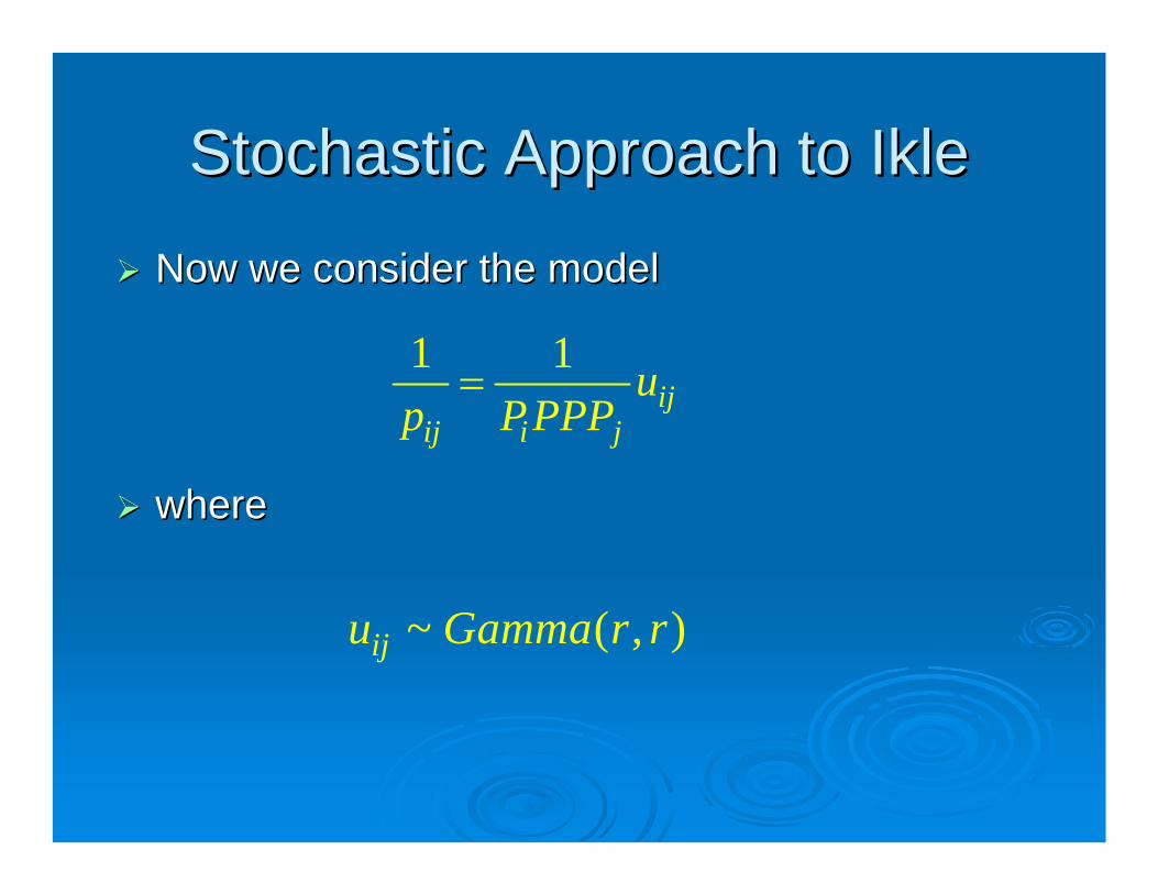
Stochastic Approach to Stochastic Approach to IkleIkle
Now we consider the modelNow we consider the model
wherewhere
1 1ij
ij i ju
p PPPP=
~ ( , )iju Gamma r r

First Order ConditionsFirst Order Conditions
Applying a weighted maximum likelihood we Applying a weighted maximum likelihood we obtain the following first order conditionsobtain the following first order conditions
i.e. i.e. IkleIkle’’ss IndexIndex
1
1 Ni
ijj iji
P wPPP P=
⎛ ⎞= ⎜ ⎟⎜ ⎟
⎝ ⎠∑
*
1
1 Mj
iji ijj
PPPw
P p=
⎛ ⎞= ⎜ ⎟⎜ ⎟
⎝ ⎠∑

Standard ErrorsStandard Errors
Computation of standard errors is an important Computation of standard errors is an important motivation for considering stochastic approach.motivation for considering stochastic approach.An MAn M--Estimator is defined as an estimator that Estimator is defined as an estimator that maximizesmaximizes
It has the following asymptotic distributionIt has the following asymptotic distribution
wherewhere
1
1( ) ( , )N
N i i ii
Q h yN =
= ∑θ x ;θ
0 0 0 0ˆ( ) [ , ]dN N − −− ⎯⎯→ 1 1θ θ 0 A B A
0
01
1plimN
i
i
hN =
∂=
∂ ∂∑2
θ
Aθ' θ
00
01
1plimN
i i
i
h hN =
∂ ∂=
∂ ∂∑θ θ
Bθ θ'
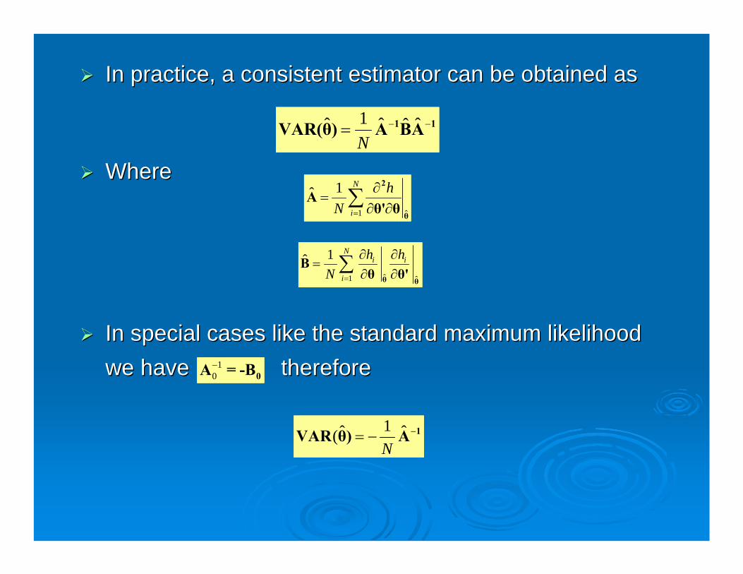
In practice, a consistent estimator can be obtained asIn practice, a consistent estimator can be obtained as
WhereWhere
In special cases like the standard maximum likelihood In special cases like the standard maximum likelihood we havewe have thereforetherefore
1ˆ ˆ ˆˆN
− −= 1 1VAR(θ) A BA
1 ˆ
1ˆN
i
hN =
∂=
∂ ∂∑2
θ
Aθ' θ
ˆ1 ˆ
1ˆN
i i
i
h hN =
∂ ∂=
∂ ∂∑θ θ
Bθ θ'
1ˆ ˆ(N
−= − 1VAR θ) A
10−
0A = -B

Many software report this as their default Many software report this as their default variance estimatorvariance estimatorThis Variance is not valid in our context This Variance is not valid in our context and the general formula should be usedand the general formula should be usedFor example if we apply to a weighted For example if we apply to a weighted linear model (e.g. CPD)linear model (e.g. CPD)
But if we apply the general formulaBut if we apply the general formula
2ˆ( σ −= 1VAR θ) (X'ΩX)
2ˆ( ' 'σ − −= 1 1VAR θ) (X'ΩX) (X Ω ΩX)(X'ΩX)

Application to OECD countriesApplication to OECD countries
OECD data from 1996. OECD data from 1996. The price information was in the form of The price information was in the form of PPPsPPPs at at the basic heading level for 158 basic headings, the basic heading level for 158 basic headings, with US dollar used as the numeraire currency. with US dollar used as the numeraire currency. The estimates of The estimates of PPPsPPPs based on the new index, based on the new index, IkleIkle’’ss and the weighted CPD for 24 OECD and the weighted CPD for 24 OECD countries along with their standard errors are countries along with their standard errors are presented in the following table.presented in the following table.

1.001.001.00USA
0.0961.2950.0941.2290.0901.168CAN
14.780192.39214.282187.42913.622182.031JAP
0.1151.5960.1131.5300.1111.464NZL
0.1041.4070.1031.3330.0991.264AUS
506.9916357.003544.9076321.42579.1286304.23TUR
0.7649.6420.7369.2380.6848.807NOR
6.81092.3296.97589.5417.00086.828ICE
0.4627.0700.4536.5980.4326.159FIN
0.74210.7580.72010.0750.6869.424SWE
0.1802.3200.1772.1830.1682.050SUI
0.94814.7280.92813.7300.88112.770AUT
12.002130.31710.994129.03710.400126.043PRT
8.738124.7998.606118.5468.304112.414SPA
14.005196.64013.891188.48213.452180.470GRC
0.6319.7620.6159.1310.5868.525DNK
0.0600.6960.0550.6690.0510.637IRE
0.0450.6820.0440.6420.0430.603UK
2.70038.1912.61835.8162.48833.578LUX
2.72840.4502.69837.8902.57735.491BEL
0.1562.2050.1552.0560.1501.921NLD
119.1961584.381115.5091504.02109.7271425.96ITA
0.4667.0350.4556.5540.4296.092FRA
0.1472.1870.1442.0340.1361.887GER
S.E.PPPS.EPPPS.EPPP
IkleCPDNew Index
MLE EstimatesCountry

Derivation of GearyDerivation of Geary--KhamisKhamis Method from CPD Method from CPD modelmodel
Recall that Geary (1958) and Khamis (1970) index is given by:
1
1
( ) /M
ij ij jj
i M
ijj
p q PPPP
q
=
=
=∑
∑1
1
N
ij iji
j N
i iji
p qPPP
P q
=
=
=∑
∑
Rao and Selvanathan (1994) used a conditional regression model to derive standard errors for PPPs.
Diewert (2005) derived G-K PPPs using stochastic approach
Here, we show that the G-K method is related to the CPD model and G-K PPPs are indeed Method of Moments estimators of PPPs from the CPD model!

Estimation of NonEstimation of Non--additive Modelsadditive Models
We consider the CPD model: We consider the CPD model:
ij i j ijp P PPP u=We show that this is a nonWe show that this is a non--additive regression model with additive regression model with ppijijas the dependent as the dependent variable,variable,yy, the country and product dummy , the country and product dummy variables as variables as regressorsregressors, , XX, and , and PPii and and PPPPPPjj as the parameter as the parameter vector, vector, ββ..Then a nonThen a non--linear modellinear model
iii uyr =β),x,(
is said to be non-additive if it cannot be written as:
iii ugy =− β),x(

Estimation of NonEstimation of Non--additive Modelsadditive Models
The nonThe non--linear least squares estimator of the linear least squares estimator of the parameters of nonparameters of non--additive models are not additive models are not consistent.consistent.The method of moments estimator may be The method of moments estimator may be considered in this case. Consider a set of moment considered in this case. Consider a set of moment conditions:conditions:
0uβ)R(x, =)( 'Ewhere R is a matrix representing K moment conditions.
The method of moments estimator is obtained by solving the sample moment conditions:
0)βX,r(y,)βR(X, =ˆˆ1 '
N

Estimation of NonEstimation of Non--additive Modelsadditive Models
The method of moments estimator is The method of moments estimator is asymptotically normal with variance matrixasymptotically normal with variance matrix
[ ] [ ] 112 ˆ'ˆˆ'ˆˆ'ˆˆ)ˆ(−−
= DRRRRDβ σMMVar
where
βββ)X,r(y,D
ˆ'
ˆ∂
∂= )βR(X,R ˆˆ = and N
u'u ˆˆˆ 2 =σ
The most efficient choice of moment conditions is
⎥⎦
⎤⎢⎣
⎡∂
∂= X
ββX,r(y,β)R(X, |)'* E
In our case, this choice leads to the unweighted index.

GK Index as a method of moments estimatorGK Index as a method of moments estimator
The CPD model isThe CPD model is
*=ij i j ijp PPPP u with 1)( * =ijuE
We rewrite the CPD model as a nonWe rewrite the CPD model as a non--additive modeladditive model
1− =ijij
i j
pu
PPPPwith 0)( =ijuE
We consider two sets of moment conditions: (i) We consider two sets of moment conditions: (i) optimal set; and (ii) weighted moment conditionsoptimal set; and (ii) weighted moment conditions

Optimal method of moments estimatorOptimal method of moments estimator
Considering the CPD model:Considering the CPD model:
1ijij ij
i j
pr u
PPPP= − =
and deriving the moment conditions leading to optimal estimator, we have the moment conditions defined by the matrix R which is defined as:
⎥⎥⎥⎥⎥⎥⎥⎥⎥⎥⎥⎥⎥⎥⎥⎥
⎦
⎤
⎢⎢⎢⎢⎢⎢⎢⎢⎢⎢⎢⎢⎢⎢⎢⎢
⎣
⎡
−−
−−
−−−
−−−
=
2211
1
21
12
11
11
22
22
12
1
21
1
22
1
12
12
1
11
...0........0
......
0..........0..
......
...
.
....
'
mn
nm
m
m
n
n
mn
nm
n
n
n
n
m
m
PPPPp
PPPPp
PPPPp
PPPPp
PPPPp
PPPPp
PPPPp
PPPPp
PPPPp
PPPPp
ER

Optimal method of moments estimatorOptimal method of moments estimator
Noting that:Noting that: 1⎡ ⎤
=⎢ ⎥⎢ ⎥⎣ ⎦
ij
i j
pE
PPPP
and using the moment conditions '( )E r =R(x,β) 0
we have the following normal equations to solve.
1
1
1 1 0
1 1 0
Mij
i jji
Nij
i jij
pPPPPP
pPPPPPPP
=
=
⎧ ⎛ ⎞− − =⎪ ⎜ ⎟⎜ ⎟⎪ ⎝ ⎠⎨
⎛ ⎞⎪− − =⎜ ⎟⎪ ⎜ ⎟
⎝ ⎠⎩
∑
∑⇒
These are exactly the same equations that define the arithmetic index introduced earlier.
Estimated standard errors can be computed by substituting the MOM estimator in the formula for the asymptotic variance.
1
1
1
1
mij
ijj
nij
jii
pP
m PPP
pPPP
n P
=
=
⎧ ⎛ ⎞=⎪ ⎜ ⎟⎜ ⎟⎪ ⎝ ⎠⎨
⎛ ⎞⎪= ⎜ ⎟⎪
⎝ ⎠⎩
∑
∑

GearyGeary--KhamisKhamis method as a method of moments method as a method of moments estimatorestimator
We consider weighted moment conditions where We consider weighted moment conditions where quantities are used as weights.quantities are used as weights.
and deriving the moment conditions leading to optimal estimator, we have the moment conditions defined by the matrix R which is defined as:
⎥⎥⎥⎥⎥⎥⎥⎥⎥⎥⎥⎥⎥⎥⎥⎥
⎦
⎤
⎢⎢⎢⎢⎢⎢⎢⎢⎢⎢⎢⎢⎢⎢⎢⎢
⎣
⎡
−−
−−
−−−
−−−
=
m
nnm
m
m
nn
n
nm
n
n
n
n
n
m
PPPPq
PPPPq
PPPPq
PPPPq
Pq
Pq
Pq
Pq
Pq
Pq
...0........0
......
0....0...
...
.
...
11
1
1
1
111
21
1
1
12
1
11
R'
11
1 1
12
2 1
1
1
1nm
n m
pP PPP
pP PPP
r
pP PPP
⎡ ⎤−⎢ ⎥⎢ ⎥⎢ ⎥
−⎢ ⎥⎢ ⎥⎢ ⎥⎢ ⎥⎢ ⎥⎢ ⎥⎢ ⎥
= ⎢ ⎥⎢ ⎥⎢ ⎥⎢ ⎥⎢ ⎥⎢ ⎥⎢ ⎥⎢ ⎥⎢ ⎥⎢ ⎥
−⎢ ⎥⎣ ⎦
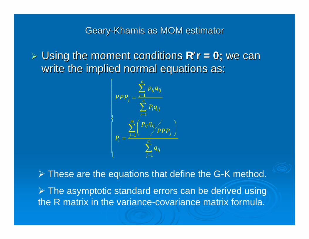
GearyGeary--KhamisKhamis as MOM estimatoras MOM estimator
Using the moment conditions Using the moment conditions RR′′rr = 0; = 0; we can we can write the implied normal equations as:write the implied normal equations as:
1
1
1
1
=
=
=
=
⎧⎪⎪ =⎪⎪⎪⎨
⎛ ⎞⎪ ⎜ ⎟⎪ ⎝ ⎠=⎪
⎪⎪⎩
∑
∑
∑
∑
n
ij iji
j n
i iji
mij ij
jji m
ijj
p qPPP
P q
p qPPP
Pq
These are the equations that define the G-K method.
The asymptotic standard errors can be derived using the R matrix in the variance-covariance matrix formula.

MOM estimators of MOM estimators of PPPsPPPs and SEand SE’’s s –– OECD ExampleOECD Example
0.1151121.2714410.0900.0856951.16CAN
15.83708179.004813.62212.52263181JAP
0.1400981.5450690.1110.1068931.455NZL
0.1069961.3511730.0990.085981.259AUS
549.12215967.556579.128393.97446251TUR
0.7647489.1193350.6840.4576668.751NOR
9.47338990.028537.0006.14221186.15ICE
0.6384996.8957260.4320.4045936.12FIN
1.02458310.560690.6860.7267019.382SWE
0.1796082.2200590.1680.1463312.037SUI
1.09832814.402640.8810.73126612.71AUT
9.307088124.774510.4006.56711125.4PRT
10.59001122.17128.3047.726502111.8SPA
13.14857187.335213.4529.271153179.5GRC
0.8726699.4577030.5860.5918078.481DNK
0.0565690.6577540.0510.0377090.633IRE
0.0537610.6795640.0430.0363110.5996UK
3.44616536.78772.4882.45426933.35LUX
2.70086738.704362.5771.94612535.3BEL
0.1566022.0321610.1500.111561.909NLD
129.50461537.168109.72779.253371419ITA
0.5161946.6794910.4290.6067556.067FRA
0.154742.083160.1360.1094421.878GER
GMM SE G-KG-K
Index
MLE SEArithematic
GMM SE ArithmeticArithmetic Index

ConclusionConclusionA new system for international price comparison is A new system for international price comparison is proposed. Existence and uniqueness establishedproposed. Existence and uniqueness establishedA stochastic framework for generating the Rao, A stochastic framework for generating the Rao, IkleIkle and and the new index has been established.the new index has been established.Using the framework of MUsing the framework of M--estimators, standard errors estimators, standard errors are obtained for the are obtained for the PPPsPPPs from each of the methods. from each of the methods. The GearyThe Geary--KhamisKhamis method is shown to be a Method of method is shown to be a Method of moments estimator of moments estimator of PPPsPPPs in the CPD model. Standard in the CPD model. Standard errors for the GK estimator are obtained.errors for the GK estimator are obtained.Empirical application using the OECD data generates Empirical application using the OECD data generates PPPsPPPs from different methods along with their standard from different methods along with their standard errors.errors.Further work is necessary to address the problem of Further work is necessary to address the problem of choosing between different stochastic specifications.choosing between different stochastic specifications.


![[Karl Terzaghi Ralph B Peck Gholamreza Mesri]Soil Mechanics in Engineering Practice 3rd Edition[Engineersdaily.com]](https://img.pdfslide.us/doc/110x75/563db949550346aa9a9bd992/karl-terzaghi-ralph-b-peck-gholamreza-mesrisoil-mechanics-in-engineering.jpg)