Systems Biology – Signaling Motifsweb.iitd.ac.in/~sumeet/IIT_Talk_SIGNET-TALK-FINAL.pdf · Systems Biology – Signaling Motifs . Sniffers, Buzzers, blinkers, Toggle switch and

Systems Biology – Signaling Motifs

Sniffers, Buzzers, blinkers, Toggle switch and Oscillations

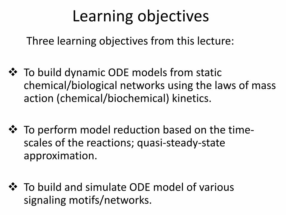
Learning objectives Three learning objectives from this lecture: To build dynamic ODE models from static

chemical/biological networks using the laws of mass action (chemical/biochemical) kinetics.

To perform model reduction based on the time-

scales of the reactions; quasi-steady-state approximation.

To build and simulate ODE model of various

signaling motifs/networks.

References

John J Tyson, Katherine C Chen and Bela Novak, Sniffers, buzzers,toggles and blinkers: dynamics of regulatory and signaling pathwaysin the cell, Current Opinion in Cell Biology 2003, 15:221231.

Mathematical Modeling in Systems Biology - An Introduction, BrianP. Ingalls, MIT Press (2013).

Biochemical Oscillations and Cellular Rhythms: The Molecular Basesof Periodic and Chaotic Behaviour, Albert Goldbeter (1996).

K. Sriram (IIIT-Delhi) NNMCB-1 December 21, 2014 3 / 33

Why model biological/chemical reaction networks?

With the advent of new biotechnological techniques it is possible todissect the molecular mechanisms that underlie the adaptive behaviorof living cells. Examples are cell-division cycle, lytic-lysogenic switchof virus etc.

The information of the molecular mechanisms are laid down in theform of graphical form. For example, http://www.biocarta.com/;http://discover.nci.nih.gov/mim/kohnk/kohnk.jsp

In these graphical forms, genes, proteins and metabolites are hookedtogether by chemical reactions and intermolecular interactions.

The temptation is irresistible to ask whether physiological regulatorysystems can be understood in mathematical terms.


Biological Networks - constructed from simpler modules

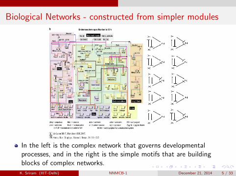
In the left is the complex network that governs developmentalprocesses, and in the right is the simple motifs that are buildingblocks of complex networks.


Signalling responses of motifs in a network

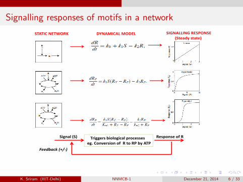
STATIC NETWORK DYNAMICAL MODEL SIGNALLING RESPONSE(Steady state)

Triggers biological processesSignal (S) Response of RTriggers biological processeseg. Conversion of R to RP by ATP

Feedback (+/‐)


Usefulness of mathematical models in analyzing biologicalnetworks

Account for experimental observations and to determine the validityof experimental conclusions.

Clarification of hypothesis.

Difficult to rely only on intuition. Mathematical equations provides astrong foundation for validating concepts and analyze complex datathat involves multiple coupled variables.

Models identify critical parameters for which certain phenomena canoccur. For eg., switch-like behavior, oscillations etc.


Usefulness and cons of mathematical models

Different regulatory mechanisms can be explored through models fromwhich only plausible mechanisms can be identified, which otherwiseare expensive and time consuming to carry out through experiments.

Models can help to identify different dynamically important regimes,which may be hard or inaccessible to experimentalists.

Problems: When the numbers become small, differential equationdescriptions breaks down.

Estimating kinetic parameters becomes difficult if ODE models arehigh dimensional.


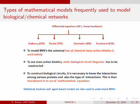
Types of mathematical models frequently used to modelbiological/chemical networks


Chemical/Biological reaction networks – What is it?

Species‐1

Species 3

Species‐4

Species‐3

Complex

Species‐2 Species‐5

Closed reaction network Open reaction network

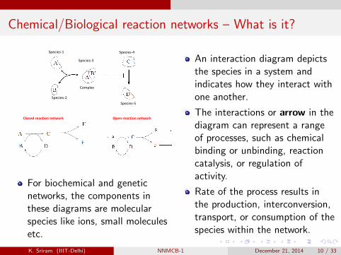
For biochemical and geneticnetworks, the components inthese diagrams are molecularspecies like ions, small moleculesetc.

An interaction diagram depictsthe species in a system andindicates how they interact withone another.

The interactions or arrow in thediagram can represent a rangeof processes, such as chemicalbinding or unbinding, reactioncatalysis, or regulation ofactivity.

Rate of the process results inthe production, interconversion,transport, or consumption of thespecies within the network.


Writing rate laws, stoichiometry and evolution ofconcentration in chemical reaction networks

Consider the following reactions (i) A + B → C + D, (ii) 3 A + B →A + C and (iii) A + 2 B → 3A + c.

Assume k to be the rate constant of the all the reactions.

What is the rate law, ’v’ for the reaction?

What are the stoichiometric coefficients for the reaction?

What is the integrated rate law (or) evolution of the concentration foreach of the reactions?


Solution - (i)

The rate of irreversible reaction is given as v = k [A][B].

The evolution equations or the concentration variations in time forthe reactant [A], [B], and the products [C] and [D] are given as d [A]

dt ,d [B]dt , d [C ]

dt , d [D]dt .

Stoichiometric coefficients for A, B, C, D are -1, -1, 1, and 1respectively.

The evolution /integrated rate laws of the species depends on the rate

– d [A]dt = –d [B]

dt = vd [C ]dt = d [D]

dt = v

Note the signs; -ve for reactant & +ve for product.


Solution - (ii)

The rate of the reaction 3 A + B → A + C is given as v = k[A]3[B].

When we write the evolution of the concentration of A, we must takeinto consideration the fact that each time this reaction occurs, onlytwo molecules of A are transformed (one is conserved). So, thevariation of A is given by−1

2d [A]dt = v = k [A]3[B].

The coefficient 3 is the balance for the species A in reaction and thesign - stands because, globally, A is transformed (not produced).

Three things are vital to write a correct rate laws for a given reaction:(i) Sign, (ii) Stoichiometric coefficient, & (iii) Rate, v.


Solution - (iii)

For the reaction A + 2 B → 3A + C, the stoichiometric coefficientsareηA = 3 – 1 = 2, ηB = 0 – 2 = -2, ηC = 1 – 0 = 1.

So – d [A]dt = ηA k[A][B]2 = 2k [A][B]2

–d [B]dt = ηBk [A][B]2 =2k [A][B]2

d [C ]dt = ηCk[A][B]2 = k[A][B]2

In general, for the reaction n X + ......... p X, the vectorial form of

the equation isd [X ]

dt= ηv ,with η = p − n .

η is called the stoichiometric coefficient. The coefficient is positive if,globally, the species is produced (p > n), and negative if the speciesis transformed (n > p).


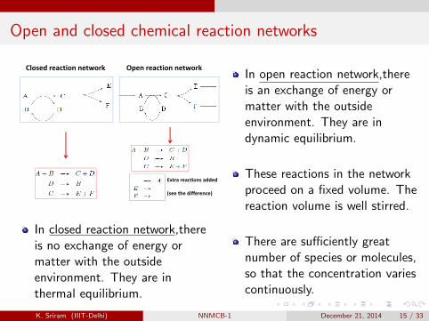
Open and closed chemical reaction networks

Closed reaction network Open reaction network

Extra reactions added

(see the difference)

In closed reaction network,thereis no exchange of energy ormatter with the outsideenvironment. They are inthermal equilibrium.

In open reaction network,thereis an exchange of energy ormatter with the outsideenvironment. They are indynamic equilibrium.

These reactions in the networkproceed on a fixed volume. Thereaction volume is well stirred.

There are sufficiently greatnumber of species or molecules,so that the concentration variescontinuously.


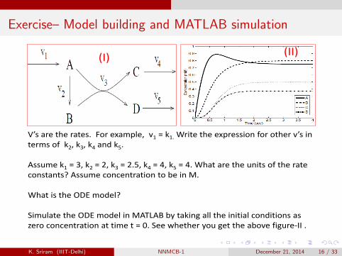
Exercise– Model building and MATLAB simulation

(I) (II)

V’s are the rates. For example, v1 = k1. Write the expression for other v’s in terms of k2, k3, k4 and k5.

Assume k1 = 3, k2 = 2, k3 = 2.5, k4 = 4, k5 = 4. What are the units of the rate constants? Assume concentration to be in M.

What is the ODE model?

Simulate the ODE model in MATLAB by taking all the initial conditions as zero concentration at time t = 0. See whether you get the above figure‐II .


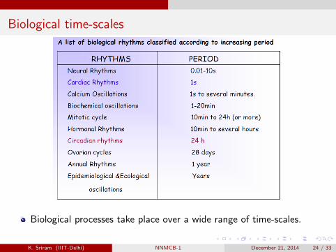
Biological time-scales

Biological processes take place over a wide range of time-scales.


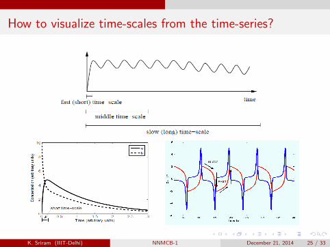
How to visualize time-scales from the time-series?


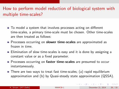
How to perform model reduction of biological system withmultiple time-scales?

To model a system that involves processes acting on differenttime-scales, a primary time-scale must be chosen. Other time-scalesare then treated as follows:

Processes occurring on slower time-scales are approximated asfrozen in time.

Elimination of slow time-scales is easy and it is done by assigning aconstant value or as a fixed parameter.

Processes occurring on faster time-scales are presumed to occurinstantaneously.

There are two ways to treat fast time-scales; (a) rapid equilibriumapproximation and (b) by Quasi-steady state approximation (QSSA).


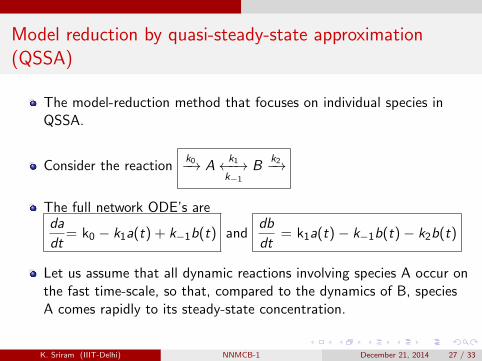
Model reduction by quasi-steady-state approximation(QSSA)

The model-reduction method that focuses on individual species inQSSA.

Consider the reactionk0−→ A

k1←−→k−1

Bk2−→

The full network ODE’s areda

dt= k0 − k1a(t) + k−1b(t) and

db

dt= k1a(t)− k−1b(t)− k2b(t)

Let us assume that all dynamic reactions involving species A occur onthe fast time-scale, so that, compared to the dynamics of B, speciesA comes rapidly to its steady-state concentration.


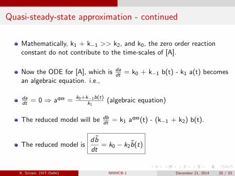
Quasi-steady-state approximation - continued

Mathematically, k1 + k−1 >> k2, and k0, the zero order reactionconstant do not contribute to the time-scales of [A].

Now the ODE for [A], which is dadt = k0 + k−1 b(t) - k1 a(t) becomes

an algebraic equation. i.e.,

dadt = 0 ⇒ aqss = k0+k−1b(t)

k1(algebraic equation)

The reduced model will be dbdt = k1 aqss(t) - (k−1 + k2) b(t).

The reduced model isdb̃

dt= k0 − k2b̃(t)


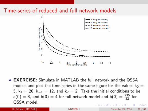
Time-series of reduced and full network models

EXERCISE: Simulate in MATLAB the full network and the QSSAmodels and plot the time series in the same figure for the values k0 =5, k1 = 20, k−1 = 12, and k2 = 2. Take the initial conditions to bea(0) = 8, and b(0) = 4 for full network model and b(0) = 235

32 forQSSA model.


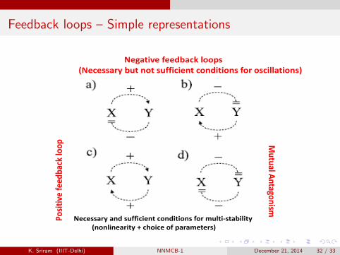
Feedback loops – Simple representations

Negative feedback loops(N b t t ffi i t diti f ill ti )(Necessary but not sufficient conditions for oscillations)

oop M

edba

ck lo

Mutual An

itive fe

e ntagonisPo

s sm

Necessary and sufficient conditions for multi‐stability(nonlinearity + choice of parameters)


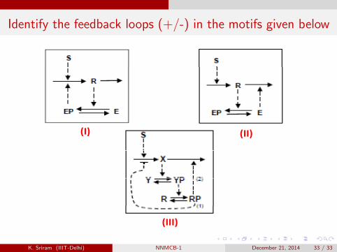
Identify the feedback loops (+/-) in the motifs given below

(I) (II)

(III)


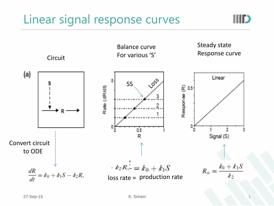
Linear signal response curves

27-Sep-15 K. Sriram 1

Circuit

Balance curve For various ‘S’

Steady state Response curve

Convert circuit to ODE

production rate loss rate =

SS

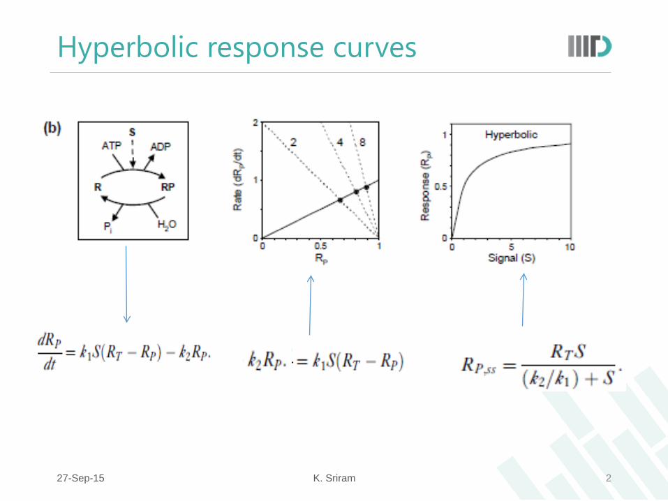
Hyperbolic response curves


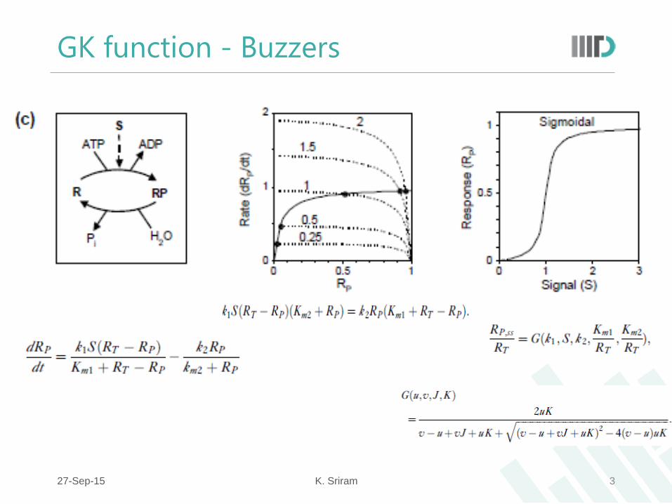
GK function - Buzzers


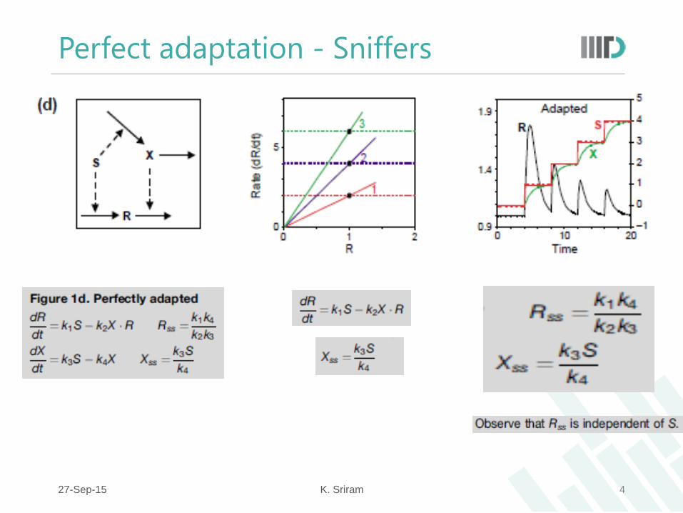
Perfect adaptation - Sniffers


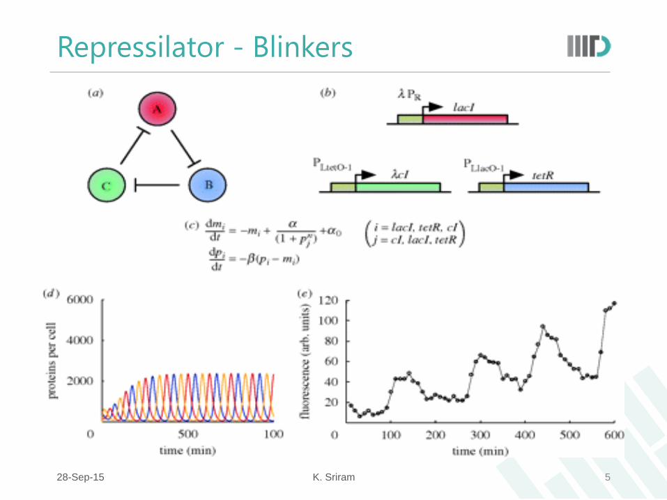
Repressilator - Blinkers


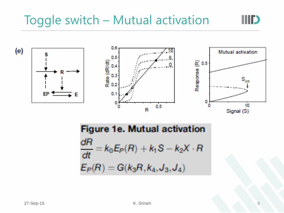
Toggle switch – Mutual activation


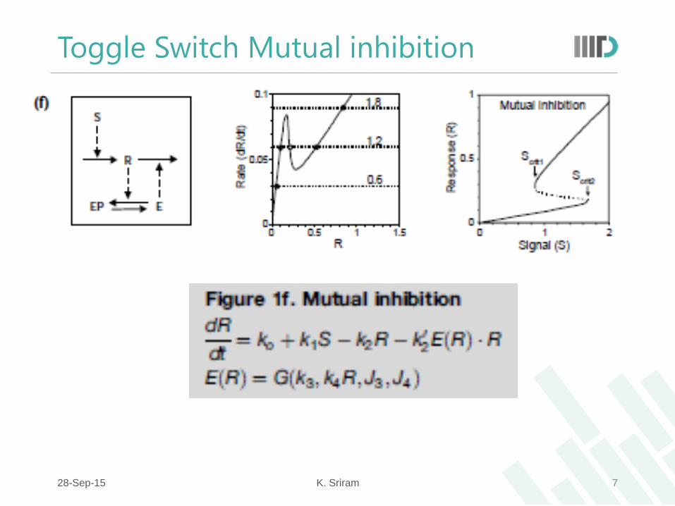
Toggle Switch Mutual inhibition


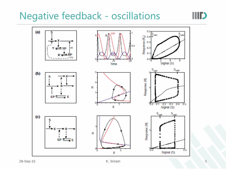
Negative feedback - oscillations


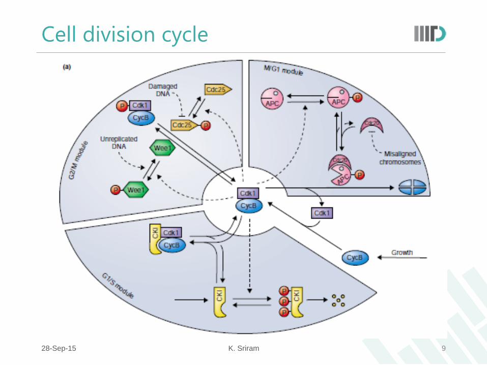
Cell division cycle


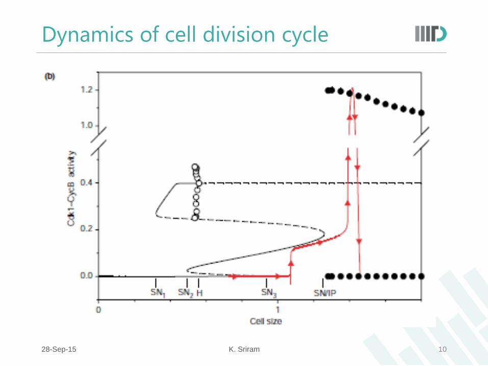
Dynamics of cell division cycle


Documents

Systems Biology – Signaling Motifsweb.iitd.ac.in/~sumeet/IIT_Talk_SIGNET-TALK-FINAL.pdf · Systems Biology – Signaling Motifs . Sniffers, Buzzers, blinkers, Toggle switch and