Systems Biology in an Imperfect World: Modeling Biological ...Systems Biology in an Imperfect World: Modeling Biological Systems with Incomplete Information Revonda M. Pokrzywa ABSTRACT

Systems Biology in an Imperfect World: Modeling Biological Systems withIncomplete Information

Revonda M. Pokrzywa

Dissertation submitted to the faculty of the Virginia Polytechnic Institute and State University in partial fulfillment of the requirements for the degree of

Doctor of PhilosophyIn

Genetics, Bioinformatics, and Computational Biology

Pedro Mendes, ChairIna HoescheleT.M. Murali

Reinhard LaubenbacherVladimir Shulaev

October 8, 2009Blacksburg, Virginia

Keywords: Biological Networks, Metabolomics, Systems Biology

Copyright 2009, Revonda M. Pokrzywa

Systems Biology in an Imperfect World: Modeling Biological Systems withIncomplete Information

Revonda M. Pokrzywa

ABSTRACT

One of the primary goals of systems biology is to understand the complex underlying network of biochemical interactions which allow an organism to respond to environmental stimuli. Models of these biological interactions serve as a tool to both codify current understanding of these interactions as well as a starting point for scientific discovery. Due to the massive amount of information which is required for this modeling process, systems biology studies must often attempt to construct models which reflect the whole of the system while having access to only partial information. In some cases, the missing information will not have a confounding effect on the accuracy of the model. In other cases, there is the danger that this missing information will make the model useless.

The focus of this thesis is to study the effect which missing information has on systems level studies within several different contexts. Specifically, we study two contexts : when the missing information takes the role of incomplete molecular interaction network knowledge and when it takes the role of unknown kinetic rate laws. These studies yield interesting results. We show that when metabolism is isolated from gene expression, the effects are not limited to those reactions under strong control by gene expression. Thus, incomplete understanding of molecular interaction networks may have unexpected effects on the resulting analysis. We also reveal that under the conditions of the current study, mass action was shown to be the superior substitute when the true rate equations for a biological system are unknown.

In addition to studying the effect of missing information in the aforementioned contexts, we propose a method for limiting the parameter search space of biochemical systems. Even in ideal scenarios where both the molecular interaction network and the relevant kinetic rate equations are known, obtaining appropriate estimates for the unknown system parameters can be challenging. By employing a method which limits the parameter search space, we are able to acquire estimates for parameter values which are much closer to the true values than those which could be obtained otherwise.

Acknowledgments

There are many people to whom I would like to express gratitude. In particular, I would

like to thank my adviser Dr. Pedro Mendes. It has been an incredible honor working for

him and I owe most of the ideas expressed in this thesis to our discussions. I would also

like to thank my advisory committee members: Dr. Ina Hoeschele, Dr. Reinhard

Laubenbacher, Dr. Vladimir Shulaev and Dr. T. M. Murali. All of my committee members

have helped me both to ask better questions as well as to search out better answers. It has

helped me immensely to have access to their expertise in my studies.

I would also like to thank the various members of the Mendes and Shulaev labs. Dr. Joel

Shuman and Dr. Diego Cortes helped me learn first hand about metabolomics. Dr.

Stephan Hoops and Dr. Bharat Mehrotra aided by adding their valuable input to

discussions about my projects. I would also like to thank Hui Cheng and Dr. Ana Martins,

who were my friends.

I owe much to the friends and family who have supported me through the years. In

particular, my sister Amanda Pokrzywa and Richard Phipps. Would also like to thank

Nicole and Alan House, Jessica Simo, Laura Cunningham, Casey Erlbaum, Sarah

Thomas, Jenni O'Brien, Jason and Erin MacEntee, Tarek Rogers, Marcia Toms, Maria

Marcus, Dennie Munson, Cary Reed, Suzanne Santamaria, the Festins, my parents John

and Kaye Pokrzywa, my grandparents Dan and Carolyn Spencer, Ramona and Henry

Spencer, and my brother John Pokrzywa.

Funding for the research undertaken was generously provided by

The National Science Foundation Grant (grant DBI-0109732 from the Plant Genome

Program, awarded to Dr. P. Mendes) and by the Virginia Bioinformatics

Institute. Additional funding was also provided by the Virginia Bioinformatics Institute as

a Bioinformatics Fellowship and as a Transdisciplinary Team Science Fellowship.

Thank you!

iii

Table of Contents

Acknowledgments …............................................................................................iii

1 Introduction ….......................................................................................................1

Background..............................................................................................................1

Introduction to Later Chapters.................................................................................7

2 The Effect of Studying Metabolism Isolated from Gene Expression..............10

Background............................................................................................................10

Materials and Methods...........................................................................................11

Results and Discussion..........................................................................................28

Conclusions............................................................................................................45

3 A Comparison of Generalized Kinetic Rate Laws...........................................47

Background............................................................................................................47

Materials and Methods...........................................................................................57


Conclusions...........................................................................................................75

4 Reducing the Search Space in Parameter Estimation for Biochemical

Networks...........................................................................................................................76

Introduction............................................................................................................76

Method...................................................................................................................78


Conclusions............................................................................................................95

5 Conclusions and Future Directions....................................................................97

Introduction............................................................................................................97

Conclusions from Research...................................................................................97

Future Directions.................................................................................................102

Conclusion...........................................................................................................103

Bibliography.......................................................................................................105

iv

List of Figures

2.1. The Claytor Artificial Biological Network.............................13

2.2. The Isolated Metabolism Model of the Claytor Network.......16

2.3. The Global Response of the Claytor Network to a Perturbation

of M1 …..............................................................................................17

2.4. The Global Response of the Claytor Network to a Knock Out

of G16 ….............................................................................................18

2.5. The Global Response of the Claytor Network to a Perturbation

of M23 ….............................................................................................19

2.6. The Global Response of the Claytor Network to a Knock Out

of G18..................................................................................................20

2.7. Comparison of the Fits of M20, M22, M24 and M13 of Claytor

Metabolism on Experimental Data......................................................36

2.8. Comparison of the Fits of M9 and P21 of Claytor Metabolism

on Experimental Data …....................................................................38

3.1 Random Bi-Bi Sequential and Bi-Bi Ping Pong Enzyme

Mechanisms............................................................................................ ..51

4.1 Model of Kinetics of Heated Monosaccharide-casein Systems...83

4.2 Fits of Mathematical Functions to Selected Metabolite

Concentrations ….....................................................................................89

4.3 Fits of ODE functions to Triose and Melanoidin Concentrations

…...............................................................................................................91

4.4 Fits of Model to Experimental Data Under Proposed Method for

Reactions J6 and J9 …..............................................................................94

4.5 Fits of Model to Experimental Data Under Control Method for

Reactions J4 and J11 …............................................................................95

v

List of Tables

2.1 Parameters Used with each Optimization Method …..............22

2.2 Description of the Quality Bit Score …...................................27

2.3 Comparison of Two Versions of the Claytor Metabolism Model

….........................................................................................................28

2.4 Aggregate Hierarchical and Metabolic Association Scores of

Metabolic Species for M1 perturbation...............................................29


Metabolic Species for M23 perturbation.............................................30


Metabolic Species for a Knock Out of G18.........................................30


Reactions for M1 perturbation.............................................................32


Reactions for M23 perturbation...........................................................32


Reactions for a Knock Out of G18......................................................33

2.10 Residual Sum of Squares for Fits of Claytor Metabolism Model

to Varying Initial Concentrations of M1 ….........................................34


Species to M1 Experiments and Associated Fit Quality Bit

Strings .................................................................................................34


to Varying Initial Concentrations of M23 ….......................................39


Species to M23 Experiments and Associated Fit Quality Bit

Strings .................................................................................................40


to G18 Knock Out Experiment ….......................................................40

vi


Species to G18 Knock Out Experiments and Associated Fit Quality Bit

Strings ….............................................................................................41

2.16 Comparison of True Kinetic Parameters and Those Estimated

Using Claytor Metabolism Model …..................................................43

3.1 True Rate Equations for Each Reaction and the Generalized

Kinetics Equations Used to Replace Them …...........................................58

3.2 Formulas for the Specified Rate Equations …..............................59

3.3 Effectiveness of Modeling Individual Reactions With Linlog

Kinetics ….................................................................................................64

3.4 Residual Sum of Squares of Fits to Experiments Using

Convenience Kinetics Applied to Full Claytor Network...........................65

3.5 Residual Sum of Squares of Fits for Each Metabolic Species and

Associated Experimental Quality Bit Strings for Full Claytor

Network .................................................................................................. . 65

3.6 Residual Sum of Squares of Fits to Experiments Using

Convenience Kinetics Applied to Full Claytor Metabolic Network.............

…...............................................................................................................66


Associated Experimental Quality Bit Strings for Claytor Metabolic

Network Using Convenience Kinetics.......................................................67

3.8 Comparison of Convenience Kinetics Parameters Obtained Using

the Full and Metabolic Portion of the Claytor Network...........................68

3.9 Residual Sum of Squares of Fits to Experiments Using Mass

Action Kinetics Applied to Full Claytor Network …................................70


Associated Experimental Quality Bit Strings for Full Claytor Network

Using Mass Action Kinetics......................................................................70


Associated Experimental Quality Bit Strings for Claytor Metabolic

vii

Network Using Mass Action Kinetics …..................................................71


Associated Experimental Quality Bit Strings for Metabolic Portion of

Claytor Network Using Mass Action Kinetics ….....................................72

3.13 Comparison of Mass Action Kinetics Parameters Obtained Using

the Full and Metabolic Portion of the Claytor Network …......................73

3.14 Comparison of Mass Action and Convenience Kinetics Applied to

Full Claytor Network …............................................................................74

3.15 Comparison of True, Mass Action, and Convenience Kinetics

Applied to the Claytor Metabolism Model …...........................................74

4.1 Initial Concentrations for Metabolites in Two Time-course Datasets

….........................................................................................................84

4.2 The Basic Stages of the Proposed Methodological........................87

4.3 A Brief Description of Applied Optimization Methods …...........88

4.4 Quality Bit Strings for Fits of Mathematical Functions to

Metabolite Concentrations...................................................................90

4.5 True Values for Rate Law Parameters …......................................91

4.6 Parameter Estimation Results for Fitting Auxiliary ODE functions

to Time-course with an Initial Glucose Concentration of 160 mmol/mL

…..........................................................................................................92

4.7 Parameter Estimation Results for Fitting Auxiliary ODE functions

to Time-course with an Initial Glucose Concentration of 75

mmol/mL .............................................................................................92

4.8 Comparison of True and Estimated Parameters Values Obtained

from Applying the Proposed Method ….............................................93

4.9 Comparison of True and Estimated Parameters Values Obtained

from Applying the Control Method …................................................94

viii

Chapter 1: Introduction

Background

Introduction

Systems biology is a manifestation of general systems theory. General systems theory itself grew out of

the recognition that in many cases a mechanistic viewpoint was insufficient to describe the complex

actions of systems (Bertalanffy 1973). In biology, the discrepancies between the behavior of isolated

components and their actions within a cellular context can be especially stark (Kaneko 2006). In order

to address these discrepancies, a method of studying biology which took the interactions of these

components into account was necessary. Systems biology studies aim to integrate knowledge of how,

and the contexts in which, these components dynamically interact in order to gain a better

understanding of biological processes as a whole. Ultimately, these studies aim to create models which

accurately reflect the system being studied. These models must therefore take into account the

underlying complex series of dynamic molecular interactions which allow the organism to respond to a

variety of stimuli in its characteristic manner (Kitano 2002). In order to study biology in this way,

much more information must be obtained than in reductionist approaches. Systems biology studies

require that not only the components be identified and characterized (the business of molecular

biology), but also how these components interact. Although there has been much success in generating

massive amounts of 'omic data via high-throughput transcriptomics and metabolomics studies, there is

still difficulty obtaining the information necessary to build accurate biological models. This difficulty

in obtaining the necessary levels of information is due to a combination of factors including technical,

experimental as well as other limitations. In turn, this lack of complete information can result in an

inability to thoroughly determine the model parameters for the system (Kotte & Heinemann 2009 ; S.

Sahle et al. 2008). Because the ability to create biologically relevant models depends on the quality and

quantity of systems level data available, it is important to assess the effect that incomplete knowledge

may have on a systems level study.

The focus of this thesis is on determining the effect that different types of incomplete or missing

1

information can have on a systems biology study. In some cases, the form of information which is

missing may not have drastic consequences. In other instances, it may be necessary to perform

additional experiments, when possible, to improve the quality of the analysis. In the worst case

scenario, it will be difficult to impossible to determine that the information is missing and this lack will

significantly affect the outcome of the given study.

In this chapter, the importance of modeling to gain an understanding of biology is discussed. In

addition, the concept of using artificial biological networks for benchmarking the effects of missing

information on the formation of these models will be advanced. Finally an introduction to the

remaining chapters is given.

Modeling in Systems Biology

Modeling is the essence of science(Rosen 1991). Constructing models forms a pivotal role in the

process of biological inference. According to Fisher, the general inference follows three core steps: 1.

the specification of a model 2. parameter estimation and 3. estimation of precision (Fisher 1992). The

process of biological discovery traditionally follows an idealized process where a hypothesis

concerning a given system is constructed, a series of experiments are performed to test this hypothesis,

and a conclusion is made. With the advent of high-throughput experiments, this process has become

less linear. Information on multiple 'omic states of a cell may now be gathered in an unbiased manner,

making it possible to formulate hypotheses after the experimental stage. These resultant hypotheses do

not suffer from the initial selection bias that other hypotheses may have. In systems biology, models

form part of an interactive process where experimental data can be used to create new hypothetical

models or to refine aspects of a predefined model (Kell & Oliver 2004). In this manner, systems

biology models may take on the roles of both hypothesis and experiment, depending on how they are

used. Within a useful model, information is codified into a more simplified construct that allows the

basic principles governing the much more complex studied system to be identified(Wolkenhauer &

Ullah 2007). These constructs can then be used to make predictions on how the target system would

behave in a given scenario. Ideally, a model will strike a balance between simplicity and correctness.

The model should be much more simplistic than the studied system, yet retain the essential features

2

(Mendes 2001). While it is often possible to create a model that encompasses multiple aspects of the

system, including all possible minutiae will likely make the model less general as well as less tractable.

The purpose of a model is not to include all possible interactions of all possible components, but rather

to be a partial representation which can offer an explanation of which features of a system are essential

to understand it (Noble 2002).

Models of biochemical systems are usually created by following one of two distinct methodologies or

by following a hybrid of the two. In the more traditional method, referred to as the bottom-up approach,

the global model is seen as being composed of a series of distinct modular parts. These modules

represent the individual biochemical reactions of the system. In the bottom-up approach, the selected

components of the final system are first studied in vitro, where information concerning a given

enzyme's rate law is determined in isolation from all other aspects of its native system. These parameter

values are then combined with those of the other constitutive biochemical moieties to form an initial

version of the system model. The initial in vitro measurements thereby serve as an initial estimate of

the true system parameters. The model is then refined by calibrating it against in vivo measurements of

the system (for example of metabolite concentrations). The bottom-up derived model thereby assumes

a certain independence of parts and the global model is seen as arising from a combination of these.

The quality of the resultant model will depend on a number of factors, including 1) the initial selection

of variables to be included and their relative independence, 2) the accuracy of the rate laws used, 3)

how widely the incorporated kinetic values of the constituent enzymes vary from those measured in

vitro, 4) the order in which variables are added to the model, and 5) the quantity and quality of the

experiments used to calibrate the model. Due to the biased nature of a bottom-up derived model, it is

critical for the model's usefulness that the components accurately reflect the underlying biochemical

network. Any interactions which are unknown will be missed by the bottom up approach. For example,

feedback loops, if not already known, will be impossible to ascertain from the data if using a bottom-up

approach.

A more recent modeling approach has been made possible by high-throughput methods in the 'omics

disciplines. The top-down approach to modeling biochemical systems relies heavily on the availability

of large systems level experimental datasets. In top down models, as opposed to bottom-up models, the

initial model is formed in an unbiased manner based upon information gleaned from a set of 'omics

3

datasets. Unlike in the bottom up approach, top down models use only in vivo datasets . In a top-down

model, constituents are related to each other via mathematical equations. A conceptual framework for

performing top-down modeling was proposed by Mendes (Mendes 2001) . According to this

framework, the initial model represents an initial guess as to how these elements relate to each other.

The mathematical functions which approximate reaction rates in terms of the constituent elements are

then identified. Finally the model parameters are estimated based on the available data. The conceptual

model is then iteratively refined as new, relevant experimental data is added (Mendes 2001). Top down

modeling is essentially a problem of network inference. One concern about using top down modeling is

that formulating higher level cellular interactions does not necessarily mean that the correct lower order

reaction mechanisms will be identified (Noble 2002). In general there are multiple disparate models

which may explain the same datasets. Thus, determining which methods of network inference best

uncover the true underlying biological network has become a problem of great interest.

Parameter Estimation

Independent of the method used to construct a given model of a biological system, parameter

estimation is a crucial step in reconciling the model to the experimental data available. Parameter

estimation is important both at the level of the individual parameters and for the model as a whole. In

bottom up construction, parameter estimation is needed to properly assign values to the parameters of

the rate laws determined from in vitro kinetic data and to optimize the fully constructed model using

the in vivo data of the system. In particular, certain parameters that depend on the state of the system

cannot be determined separately for the model to make sense and therefore must be estimated within

the context of the full network (i.e. living organism). Models determined via top down methods rely

on parameter estimation for initial stages of their formation as well as for refinement.

Artificial Biological Networks

One of the concerns surrounding top down modeling methodologies is that it is impossible to be sure if

the resultant model formed from the available data is the correct one. There are several reasons why it

is difficult to ascertain the veracity of a given model. One of the reasons is the nature of network

4

inference itself. Network inference is a type of inductive inference, meaning that it is an attempt to

make generalizations about all possible data for a given system using only a subset of the data. The

generalization in this case is the model being formed from a given dataset that is intended to encompass

the system's behavior. While it is possible to make them mathematically rigorous, inductive inferences

are uncertain in nature (Fisher 1935). The subset which is sampled may not accurately reflect the whole

space of behaviors. The uncertainty implicit in inductive inference propagates into uncertainty within

inferred biological system models. An aspect of this uncertainty is that for any given set of systems

data, there are multiple models that will be able to explain it. Therefore, model selection is a critical

step in the top down modeling process (Burnham & Anderson 1998) . In the case of complex systems,

there will not be a global model which will accurately describe the system. While a combination of

models may help to circumvent this issue in a complex system, even this approach is not guaranteed to

work for all such systems (Rosen 1985).

Uncertainty in network inference is also related to its dependence on systems level data. Top down

modeling is data driven and therefore the quality of the resultant models is dependent to a large degree

upon the quantity and quality of data available for the given system. The issues of quantity and quality

of data also cause concerns for bottom-up modeling. Biological systems datasets are not ideal in this

respect. Results from biological experiments are not always reliable, as the techniques employed can

have inherent errors (Wimsatt 2007). For example, experimental methods to determine protein

interactions will often result in considerable numbers of both false positives and false negatives (Deane

et al. 2002) . All other techniques produce some level of noise, therefore biological data sets always

contain implicit noise which makes top down modeling challenging. The implicit noise is also due to

the stochastic nature of biological systems (Kaern et al. 2005). Unlike deterministic systems, biological

systems may not always respond identically to the same perturbation each time. Instead, biological

systems react probabilistically and the same perturbation may result in different outcomes in different

instances. This combined noise from various sources makes it difficult to extract the true biological

signal which is needed to construct accurate models.

In addition to the difficulties associated with forming models from unreliable data , there is a lack of

sufficient experimental data available to fully determine a model. In most cases, systems biology

datasets are high dimensional with low sample number. While 'omics methodologies make it possible

5

to gather information on multiple variables in each sample, gathering a sufficiently large number of

samples is problematic due to cost and logistics. These high dimensional, low sample number

experimental datasets cannot be analyzed by traditional statistical methods, because it is impossible to

'sphere the data'. Data sphering is accomplished by multiplying the data matrix by the root inverse of

the covariance matrix. If the data is normally distributed, a plot of these transformed variables would

resemble a sphere. However, in high-dimensional, low sample number datasets this process is

impossible because the required root inverse of the covariance matrix does not exist. This inverse does

not exist because the covariance matrix is not of full rank for high dimensional, low sample number

datasets. This is known as the large p, small n problem(Hall et al. 2005) . Most systems biology models

are therefore under-determined, meaning that there are many models will fit the available evidence

(Kotte & Heinemann 2009). As a result of this, many parameters within the model can take multiple

values while still agreeing with the available experimental data.

This uncertainty in top down modeling leads to a predicament. Even if a fit of the model to the data

seems good, it is still possible that the model is partially or entirely incorrect. While it is possible to use

well-studied biological systems to determine the quality of a network inference method, they are not

exempt from this problem because it is unknown if the current paradigms are true(P. Mendes et al.

2003; Camacho et al. 2007) . If an inference method conceived a result which differed from the current

paradigm, it could not necessarily be ruled out. This difference could be due to errors or insufficiencies

in the current model or models used to explain the given system.

One method to assess the uncertainty associated with top down modeling is to begin with a system

where everything is known. While this is not feasible for true biological systems, it is for artificial

biological systems. These artificial biological systems generally resemble true biological systems. In

order to be useful, they must contain features similar to their nature counterparts. If a given network

inference method performs well on data derived from an unrealistically simplistic artificial network,

there is no guarantee that it would function as accurately when confronted with the more complex

biological data. Therefore, proper design of artificial biological networks is critical for their

effectiveness. An aspect of this design is that the artificial network should mirror the type of 'omics

system that the top down modeling approach intends to model. Artificial biological systems have been

successfully utilized to benchmark a number of network inference algorithms optimized for specific

6

'omics data, in particular metabolomics and transcriptomics data. In addition to making it possible to

determine if the true model was determined, artificial biological networks can also examine the effect

that noise has on network inference algorithms. As mentioned earlier in this section, data from

biological samples is comprised of both signal and noise. It is therefore useful to determine under what

levels of noise the method can be expected to remain functional.

Introduction to Later Chapters

Incomplete Knowledge and Systems Biology

Missing and incomplete information affects all branches of science, but its influence is pervasive in

systems biology studies. Much of the influence this lack of information has over systems biology is

due to systems biology's overall goal of understanding the whole of biology. As the complexity of the

biological interactions increases, so does the amount of information which is required to identify and

characterize these interactions.

The specific aims of this thesis are 1) to address several forms of missing information in systems

biology studies, 2) to assess the effect that this form of missing or incomplete information may have

on the overall conclusions of the given study, and 3) to propose methods to minimize the effect of this

missing information in certain cases.

The Effect of Incomplete Network Information

In chapter 2, the effect that partial network information has on the ability to recover system properties

is addressed. The focus here is on assessing how studying one level of a biological system, to the

exclusion of others, may affect the interpretation of results. It is not uncommon for systems level

studies to focus on the transcriptome or the metabolome without integrating any of the other levels of

cellular organization. In chapter 2, the metabolic reactions of the Claytor artificial biological network

are studied in isolation from the full network. The Claytor artificial biological network is ideal for these

purposes because it contains many of the complex characteristics of natural biological networks, while

7

having the beneficial qualities of being fully known and much more tractable to analysis. The

metabolic reactions are studied in a manner which is parallel to metabolomics time course experiments.

However, unlike true metabolomics studies, all of the members of the metabolome are identified and

there is no noise in the measurements. These ideal measurements are used to provide estimates for the

parameters of the metabolic rate equations. In this scenario, the true structure of the rate equations is

assumed to be known. Thus, this study aims to detect neither the effects of noise nor the effect of

unknown rate equations. Instead, the study's sole intent is to determine what effect ignoring

transcriptional and translation regulation will have on the ability to correctly ascertain the true kinetic

parameters of the system. It is hypothesized that the rate equation parameters which will be most

detrimentally affected by an exclusive analysis of the metabolome will be those which are primarily

under transcriptional control. In order to test this hypothesis, a method is proposed to assess the level

and type of control each reaction is most associated with.

The Effect of Unidentified Rate Laws

In chapter 3, the effect which unidentified rate laws have on creating useful systems biology models is

discussed. Due to the prevalence of unavailable rate laws for metabolic reactions, many general

kinetics equations have been proposed. In chapter 3, three methods of generalizing kinetic rate laws are

compared using the Claytor artificial biological network mentioned above. Specifically, these methods

are: generalized mass action, linlog, and convenience kinetics. In each case, the methods are assessed

on their ability to properly fit metabolite concentration time-course data. The methods are compared

both on their ability to fit the time-course data when integrated into the full network, where the

transcriptome, metabolome, and proteome are all included, and in their ability to fit data when only the

metabolic portion of the network is assumed. In this manner, it can be determined if any of the

aforementioned methods is sensitive to partial network knowledge.

Reducing the Parameter Search Space in Biochemical Networks

One of the main steps in a systems biology study is to codify available information into a useful model.

The goal, in this case, is to integrate data and models (Krohs & Callebaut 2007). In order to accomplish

this goal, the parameters for the model must be estimated using the available data. A confounding issue

8

at this stage is the large “volume” of parameter space which must be searched through. In addition to

increasing the amount of time necessary for the optimization methods to work, increased parameter

search space can increase the likelihood of obtaining improper parameter estimates. Many systems

biology models are under-determined (Ashyraliyev et al. 2009) . This means that for the limited amount

of information available there are several models which would explain it. In chapter 3, a data-driven

method for limiting the parameter search space for biochemical networks is proposed. The proposed

method assumes that the ordinary differential equations ODEs based upon the kinetic rate laws for the

given system are known and that the only issue is properly parametrizing this model (finding the values

of its constants). The underlying premise of the model is that these ODEs may be separated by initially

substituting functions which only depend on time for the concentrations of dependent chemical species

in each equation. This method is demonstrated on an artificial metabolic network obtained from the

curated portion of the BioModels database (Le Novere et al. 2006).

Conclusions and Future Directions

In the final chapter of this thesis, the outcome of the studies in previous chapters and their implications

will be discussed. In addition, future work related to these implications will also be proposed.

9

Chapter 2: The Effect of Studying Metabolism Isolated from Gene

Expression

Background

Introduction

In many systems biology studies, the underlying network of molecular interactions that constitute gene

expression and signaling is implicit within the model. Although this information may not be explicitly

formulated in the model, assumptions of how the composite biological moieties interact imply a given

network. However, this underlying network is generally not known in its entirety. This problem is

exacerbated in models of living systems, because it may not be possible to ever know whether or not

all of the components of the complete underlying biological network have been fully identified, much

less characterized. Therefore it is almost guaranteed that any biological model ignores a number of

molecular interactions. Depending on the type of model, how it was formulated, and which framework

is used, these unknown interactions may be implicit in the model or otherwise entirely absent. While it

may not be necessary for all purposes that the underlying biochemical network be entirely known, it is

important to determine to what extent the aspects of the network which are not included affect the

outcome of a modeling study. Understanding the influence of biological interactions which are not the

focus of a study is important both in minimizing any deleterious effect they may have and in efforts to

simplify complex networks.

In this chapter, the focus in on how missing information about the network influences the ability to

estimate appropriate parameter values . In particular, it examines the case where the full metabolic

network is known, but influences from the transcriptome and proteome are not taken into account. By

using an artificial biological network, it is possible to assess the effect that studying an organism's

metabolism in isolation will have on predictions of system level properties. In order to achieve this a

computational study was carried out using a dynamic model (gold standard) that includes the

metabolome, proteome and transcriptome. This network model is used as if it was the original

biological system, and used to simulate experiments. The resulting data from these in silico

experiments is is then used to calibrate a smaller model which only includes the metabolic reactions

10

and ignores the proteome and transcriptome (reduced model). Unlike natural biological systems, the

true values of all parameters as well as all interactions of the gold standard model are known. Thus it is

possible to compare not only how well the reduced model fits the experimental data, but also how close

the estimated parameter values of the reduced model are to the true ones in the gold standard.

These in silico experiments are carried out in an ideal scenario where the true form of the kinetic rate

equations is known and there is no noise in the data. It is hypothesized that those moieties which will

have the most difficulty being fit in this scenario are those which are the most influenced by

transcriptional elements. As an extension to this reasoning, it is thought that those reactions which

contain the highest number of transcriptionally influenced members will also obtain estimates for their

parameters which are the most distinct from their true values.

Materials and Methods

Overview

In order to determine the effect that studying one aspect of a biological system in isolation could have

on the resulting analysis, the metabolic portion of an artificial biological network was extracted and

studied separately. The artificial biological network used, the Claytor network, is described in detail

later in this section. After determining the subset of reactions which constituted metabolism, their

respective kinetic parameters were estimated via least-squares fitting to the data generated in the in

silico experiments. The data fitting was carried out with distinct training and validation datasets to

prevent over-fitting. The training dataset is the only one used to adjust parameter values, while the

validation dataset is used to assess how well the model predicts the system's response to a perturbation

that was not used to fit the model. The validation set is also used as a stopping criterion, such that if at

some point in the fitting iterations, the distance between the model prediction and the validation data

starts increasing, the fitting procedure will stop. It is considered that in such a case, further refinement

of the parameter values would result in a model that fits only a particular set of data. The use of this

stopping criterion with a validation dataset thus ensures that the model extrapolates as well as possible.

After fitting the reduced model to the data from the in silico experiments (obtained with the Claytor

11

network), the resultant parameter values of the isolated metabolism were then compared to their true

counterparts in the intact Claytor network (the gold standard). It is hypothesized that those reactions

which are under primarily metabolic control would achieve more accurate parameters than those which

are under primarily transcriptional control. In order to test this hypothesis, the primary control type is

predicted for each reaction under multiple experimental conditions.

Artificial Biological Networks

Claytor Artificial Biological Network

In order to ascertain the effect that incomplete or missing information had on the systems level

analysis, the Claytor artificial biochemical network was used. The Claytor network is shown in figure

2.1 . As was mentioned previously in this chapter, artificial biological networks are important

modeling resources. Without a predefined artificial network, it would be impossible to make a

meaningful comparison between studies where all information is known and those where knowledge is

limited. Initially introduced as dream1n3 to the DREAM challenge (Stolovitzky et al. 2007;

Stolovitzky et al. 2009) as a means of benchmarking network inference, or top down modeling

methods, the Claytor network represents a small biochemical network that includes metabolism, signal

transduction, and gene regulation aspects. The Claytor artificial biological network was chosen for this

study because its complexity mirrors that of true biochemical systems, while remaining much more

tractable (e.g. it has only 20 genes).

12

Figure 2.1 The Claytor artificial biological network. Rectangle represent proteins. Red rectangles act as transcription factors, while green

ones act as enzymes or directly participate as reactants or products in reactions. Clear ellipses are external metabolites, while green

ellipses represent internal metabolites. Yellow parallelograms represent genes as mRNA concentrations. Used with permission from P.

Mendes.

Properties of the Full Claytor Network

The complete Claytor network contains 59 internal state variables, of which 16 are metabolites, 23 are

protein forms, and 20 are genes. The Claytor network also encompasses a simplified, artificial

environment. This environment encompasses 8 external metabolites which may be used to perturb the

full network in a manner reminiscent of exo-metabolite perturbations in metabolomics studies. The

metabolic and transcriptomic portions of the Claytor network follow realistic kinetics which depend on

the nature of their interactions. As a result, the kinetics of the various metabolic reactions and those

involved in transcription, translation, and degradation of proteins and mRNA encompass a wide range

of dynamic scales and steady state levels. In addition to realistic kinetics, the components of the

Claytor network are subject to both both hierarchical (gene regulation) and metabolic control.

13

The metabolic portion of the Claytor network contains subnets which are involved in the processes of

catabolism, biosynthesis of a co-factor, and redox chain reactions to remove a toxic external compound,

M1. In addition, the metabolic portion of the full Claytor network includes other features which appear

in biochemical networks but are not usually included in artificial ones. There is competition for the

main energy source, M12, between the subnets functioning in catabolism and generation of redox

potential. The redox chain, which is crucial for detoxification, contains a mixture of small molecules

and proteins that can exist in both an oxidized and reduced state.

The full Claytor network also contains signaling pathways which can sense presence of the toxic M1 or

the detoxified M3. The signaling pathways are reminiscent of those found in biochemical systems,

where receptor proteins bind to their target and form complexes, which can then act as transcription

factors.

Transcriptional control is also present in the Claytor network, beyond its role in signaling: two

additional transcription factors encode genes that are subject to regulation by other transcription

factors. Each gene codes for a specific mRNA that can produce a protein. Thus, knocking out a given

gene will have an effect on its target protein concentration. However, similar to biological systems,

several genes have redundant functions so that knocking out a given gene in the network will not

necessarily eliminate the function since there may be another protein carrying out that function (though

with different properties).

Claytor Metabolism Model

The Claytor metabolism model consists of the metabolic portion in isolation from the full network.

Unlike the complete version of the network, the Claytor metabolism model does not represent

transcriptional control. Thus, the Claytor metabolism model mirrors studies where the focus is the

metabolic portion of a system and the rest of the network is excluded (Broeckling et al. 2005; Draeger

et al. 2009; Guy et al. 2008; Moco et al. 2009). Because the true systems level properties of the entire

network are known, it is possible to quantify the effect of using only a portion of the network in an

analysis. The subset of reactions which constituted the metabolism portion were identified by

including reactions which contained metabolites. The only proteins included explicitly are those that

14

react with metabolites (in the redox cycles), the proteins that catalyze the metabolic reactions are

represented only implicitly in the kinetic parameters of the reactions, and therefore became constants of

the model. The metabolism reactions used in this study were R1, R2, R3, R4, R5, R6, R7, R8, R9, R10,

R11, R12, R13, R14, and R19. It was unclear whether or not the signaling reactions for M1 and M3

should be included as part of the metabolism set of reactions. Under transcriptional control, these

reactions act as a signaling mechanism to detect M1 and M3 levels. However, when transcriptional

regulation is removed from the model, the proteins in the reaction should act as receptors and sequester

the relevant metabolite. A comparison was made between metabolism models which contained the M1

and M3 signaling reactions and one which did not. The Akaike's information criterion (Akaike 1974),

which is described later, was used as a basis for this decision. As a result of this comparison, the model

without M1 and M3 signaling was selected. This model is depicted in figure 2.2. These reactions were

the targets for the kinetic estimation procedures in addition. They were replaced by the relevant

generalized rate laws in both the studies where the rest of the Claytor network remained intact as well

as those where only the metabolic reactions were included. Details of this comparison are in the results

and discussion section.

15

Figure 2.2 The Claytor isolated metabolism model is shown. This model consists of a subset of reactions from the Claytor network.

Gray rectangles are enzymes. Unlike the full Claytor network, these are initial enzyme concentrations and do not change. The green

rectangles are proteins which directly participate in reactions as products or reactants. Their concentrations are therefore allowed to

change. The metabolite representations are identical to those in the complete Claytor network. Clear ellipses represent external

metabolites, while green ellipses represent internal metabolites.

Datasets

Two classes of in silico "experimental" datasets were created for the purposes the current study. One set

is used as a training set for estimating kinetic parameters and in certain models estimating the initial

protein concentrations. The second set was used as a test set so that validation could be performed, thus

preventing over fitting. Validation is employed both during the process of parameter estimation, and

again to test the final model's performance on a novel dataset. In order to capture the inherent dynamics

of the system, and to parallel the types of data necessary to study biological systems, time-series

datasets were generated for both training and testing of models. These training and testing time-series

datasets were composed of both metabolic and genetic perturbations. Both the training and test

datasets were created by using the simulation package COPASI (S. Hoops et al. 2006) .

16

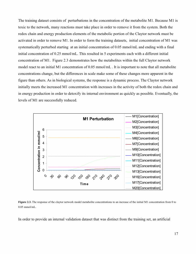
The training dataset consists of perturbations in the concentration of the metabolite M1. Because M1 is

toxic to the network, many reactions must take place in order to remove it from the system. Both the

redox chain and energy production elements of the metabolic portion of the Claytor network must be

activated in order to remove M1. In order to form the training datasets, initial concentration of M1 was

systematically perturbed starting at an initial concentration of 0.05 mmol/mL and ending with a final

initial concentration of 0.25 mmol/mL. This resulted in 5 experiments each with a different initial

concentration of M1. Figure 2.3 demonstrates how the metabolites within the full Claytor network

model react to an initial M1 concentration of 0.05 mmol/mL . It is important to note that all metabolite

concentrations change, but the differences in scale make some of these changes more apparent in the

figure than others. As in biological systems, the response is a dynamic process. The Claytor network

initially meets the increased M1 concentration with increases in the activity of both the redox chain and

in energy production in order to detoxify its internal environment as quickly as possible. Eventually, the

levels of M1 are successfully reduced.

Figure 2.3. The response of the claytor network model metabolite concentrations to an increase of the initial M1 concentration from 0 to

0.05 mmol/mL.

In order to provide an internal validation dataset that was distinct from the training set, an artificial

17

M1 Perturbation

0

1

2

3

4

5

6

0 30 60 90 120

150

180

210

240

270

300

Time

Conc

entra

tion

in m

mol

/ml

M1[Concentration]M2[Concentration]M3[Concentration]M4[Concentration]M6[Concentration]M7[Concentration]M9[Concentration]M10[Concentration]M11[Concentration]M12[Concentration]M13[Concentration]M16[Concentration]M17[Concentration]M20[Concentration]M22[Concentration]

gene knockout was created by setting the rate constant V of mRNA synthesis of gene G16 to 0. By

setting the parameter V to 0, no mRNA synthesis occurs for the selected gene. In figure 2.4, the effect

of knocking out G16 is shown. By knocking out G16, a disturbance is created in the network that is

soon compensated for by other members. Thus demonstrating the redundancy inherent in the system.

This is comparable to the effect that non-lethal gene knockouts can have in biological systems.

Figure 2.4. The effect of knocking out G16 on the dependent variable in the Claytor metabolic network is shown. In some instances, the

G16 knock out (KO) had no effect on a variable's concentration. These non-affected variables are not shown. In most of the species, the

G16 KO caused a perturbation in the earlier time points which subsided by the end of the simulation.

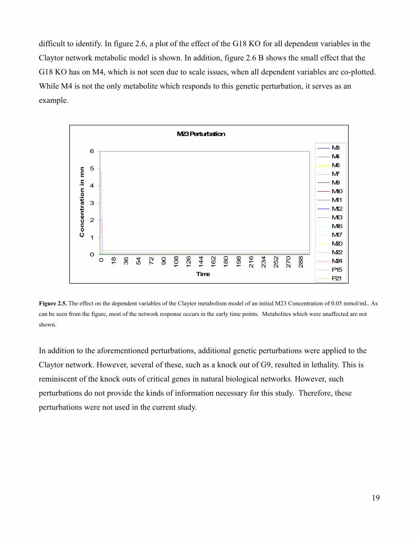
The final validation sets were composed of both metabolic and genetic perturbations. In the metabolic

perturbation, the initial concentration of metabolite M23, which serves as an energy source for the

Claytor network, is increased incrementally from 0.05 to 2.0 mmol/mL. As can be seen in figure 2.5,

even an initial M23 concentration of 0.05 mmol/mL, which is much less than the full model initial

concentration of 1 mmol/mL, results in a lot of initial activity which soon dissipates as the supply of

M23 is exhausted. The genetic perturbation consisted in a knock out of G19. This G18 knock out (KO)

was achieved in the same manner as the G16 KO which was used in the earlier model validation. The

G18 KO is more subtle as it effects metabolites which operate at different scales. Because the scales of

the effected metabolites are often much smaller than the non-affected ones, the changes can be more

18

Effect of G16 knockout

0

2

4

6

8

10

12

0 35 70 105

140

175

210

245

280

315

350

385

420

455

490

Time

Con

cent

ratio

n in

mm

ol/m

L

M24M22M16M17M13M7M6M20M12M11M10M9P21M4M3

difficult to identify. In figure 2.6, a plot of the effect of the G18 KO for all dependent variables in the

Claytor network metabolic model is shown. In addition, figure 2.6 B shows the small effect that the

G18 KO has on M4, which is not seen due to scale issues, when all dependent variables are co-plotted.

While M4 is not the only metabolite which responds to this genetic perturbation, it serves as an

example.

Figure 2.5. The effect on the dependent variables of the Claytor metabolism model of an initial M23 Concentration of 0.05 mmol/mL. As

can be seen from the figure, most of the network response occurs in the early time points. Metabolites which were unaffected are not

shown.

In addition to the aforementioned perturbations, additional genetic perturbations were applied to the

Claytor network. However, several of these, such as a knock out of G9, resulted in lethality. This is

reminiscent of the knock outs of critical genes in natural biological networks. However, such

perturbations do not provide the kinds of information necessary for this study. Therefore, these

perturbations were not used in the current study.

19

M23 Perturbation

0

1

2

3

4

5

6

0 18

36

54

72

90

108

126

144

162

180

198

216

234

252

270

288

Time

Co

ncen

trati

on

in

mm

ol/m

L M3M4M6M7M9M10M11M12M13M16M17M20M22M24P15P21

A.

B.

Figure 2.6. The effect of knocking out gene G18 on the Claytor network metabolism model. A. The effect show on all dependent

variables in the model. B. The effect of knocking out G18 demonstrated for M4.

20

Effect of G18 Knock Out

0

1

2

3

4

5

6

0 21 42 63 84105

126147

168189

210231

252273

294

Time

Co

ncen

trati

on

in

mm

ol/m

L

P15M1M3M2M4P21M9M10M11M12M20M6M7M13M17M16M22M24M23M19M18

Effect of G18 Knock Out on M4 Concentration

4.56E-05

4.56E-05

4.56E-05

4.56E-05

4.56E-05

4.57E-05

4.57E-05

4.57E-05

0 21 42 63 84 105

126

147

168

189

210

231

252

273

294

Time

Conc

entra

tion

in m

mol

/mL

M4

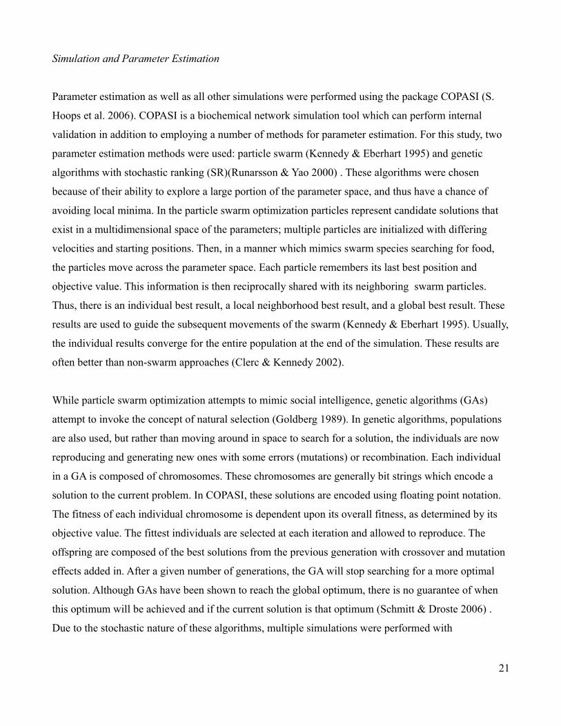
Simulation and Parameter Estimation

Parameter estimation as well as all other simulations were performed using the package COPASI (S.

Hoops et al. 2006). COPASI is a biochemical network simulation tool which can perform internal

validation in addition to employing a number of methods for parameter estimation. For this study, two

parameter estimation methods were used: particle swarm (Kennedy & Eberhart 1995) and genetic

algorithms with stochastic ranking (SR)(Runarsson & Yao 2000) . These algorithms were chosen

because of their ability to explore a large portion of the parameter space, and thus have a chance of

avoiding local minima. In the particle swarm optimization particles represent candidate solutions that

exist in a multidimensional space of the parameters; multiple particles are initialized with differing

velocities and starting positions. Then, in a manner which mimics swarm species searching for food,

the particles move across the parameter space. Each particle remembers its last best position and

objective value. This information is then reciprocally shared with its neighboring swarm particles.

Thus, there is an individual best result, a local neighborhood best result, and a global best result. These

results are used to guide the subsequent movements of the swarm (Kennedy & Eberhart 1995). Usually,

the individual results converge for the entire population at the end of the simulation. These results are

often better than non-swarm approaches (Clerc & Kennedy 2002).

While particle swarm optimization attempts to mimic social intelligence, genetic algorithms (GAs)

attempt to invoke the concept of natural selection (Goldberg 1989). In genetic algorithms, populations

are also used, but rather than moving around in space to search for a solution, the individuals are now

reproducing and generating new ones with some errors (mutations) or recombination. Each individual

in a GA is composed of chromosomes. These chromosomes are generally bit strings which encode a

solution to the current problem. In COPASI, these solutions are encoded using floating point notation.

The fitness of each individual chromosome is dependent upon its overall fitness, as determined by its

objective value. The fittest individuals are selected at each iteration and allowed to reproduce. The

offspring are composed of the best solutions from the previous generation with crossover and mutation

effects added in. After a given number of generations, the GA will stop searching for a more optimal

solution. Although GAs have been shown to reach the global optimum, there is no guarantee of when

this optimum will be achieved and if the current solution is that optimum (Schmitt & Droste 2006) .

Due to the stochastic nature of these algorithms, multiple simulations were performed with

21

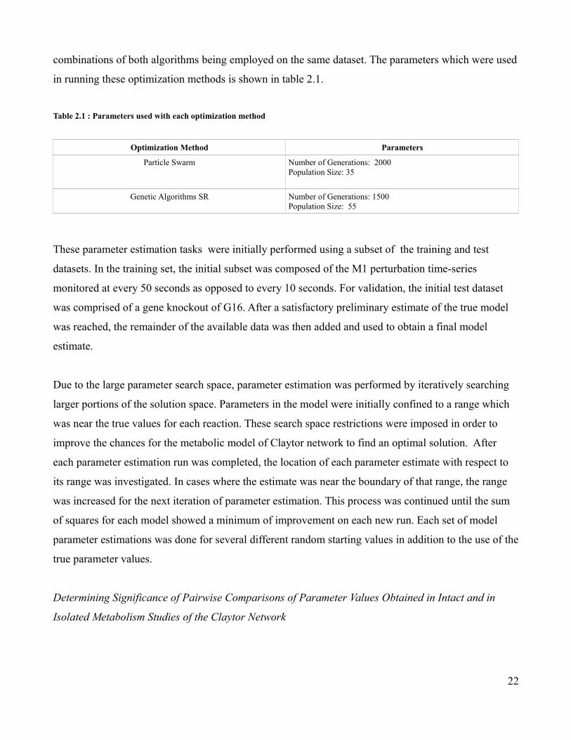
combinations of both algorithms being employed on the same dataset. The parameters which were used

in running these optimization methods is shown in table 2.1.

Table 2.1 : Parameters used with each optimization method

Optimization Method Parameters

Particle Swarm Number of Generations: 2000Population Size: 35

Genetic Algorithms SR Number of Generations: 1500Population Size: 55

These parameter estimation tasks were initially performed using a subset of the training and test

datasets. In the training set, the initial subset was composed of the M1 perturbation time-series

monitored at every 50 seconds as opposed to every 10 seconds. For validation, the initial test dataset

was comprised of a gene knockout of G16. After a satisfactory preliminary estimate of the true model

was reached, the remainder of the available data was then added and used to obtain a final model

estimate.

Due to the large parameter search space, parameter estimation was performed by iteratively searching

larger portions of the solution space. Parameters in the model were initially confined to a range which

was near the true values for each reaction. These search space restrictions were imposed in order to

improve the chances for the metabolic model of Claytor network to find an optimal solution. After

each parameter estimation run was completed, the location of each parameter estimate with respect to

its range was investigated. In cases where the estimate was near the boundary of that range, the range

was increased for the next iteration of parameter estimation. This process was continued until the sum

of squares for each model showed a minimum of improvement on each new run. Each set of model

parameter estimations was done for several different random starting values in addition to the use of the

true parameter values.

Determining Significance of Pairwise Comparisons of Parameter Values Obtained in Intact and in

Isolated Metabolism Studies of the Claytor Network

22

One of the main benefits to using an artificial biological network is that the true values of parameters

are known. This makes it possible to compare the parameter values obtained for the Claytor

metabolism model to those in the intact network. By comparing these parameters, it is possible to

assess the effect that studying the metabolome in isolation has on the analysis of the metabolic

reactions overall as well as the effect on individual reactions. In order to determine when differences

between parameter values were significant, the Wilcoxon signed rank test was employed. The

Wilcoxon signed rank test was preferred over the t-test, as it is nonparametric and does not make the

assumption of normality (Whitley & Ball 2002).

The Wilcoxon signed rank test was applied using the internal R stats package (R Development Core

Team 2009) . The two sided pairwise Wilcoxon test was used to obtain the significance of differences

between parameter values on both the overall set of reactions as well as on individual reactions. By

making these comparisons at different resolutions, it is possible to determine whether individual

reactions are more affected by studying the metabolome in isolation than others as well as to assess the

parameter differences overall.

Predicting Control Type of Differing Experiments

In biological systems, reactions are often under both transcriptional, or hierarchical, and metabolic

control (Heinrich & Schuster 1996; Kacser & JA Burns 1995; A de la Fuente et al. 2002). Depending

upon environmental conditions and the overall network structure, a given reaction may be under one

form of control more than another at a given point in time. If a given metabolic reaction is under

stronger hierarchical control during a perturbation, then it is reasonable to hypothesize that an analysis

which takes transcription into account would give more accurate results for this reaction. Similarly, an

isolated study of metabolism might be sufficient to understand reactions which are only weakly

affected by transcription. Therefore, the degree to which an isolated metabolic study may be successful

for a series of reactions should correlate to the distribution and type of control its components are

under.

In this study, the type and amount of control a metabolic reaction is under is predicted in the following

23

manner. For each dependent variable in the metabolic network, a series of p-values are calculated based

upon its Kendall's correlation (Kendall 1938) to the concentrations of predetermined transcriptional

regulatory species as well as to other metabolites. In this study, transcriptional elements are considered

to be the transcription factor and mRNA concentrations for a given experimental perturbation of the

Claytor network. The metabolic elements include all of the metabolite concentrations as well as those

of the proteins which were directly involved as substrates or products in the metabolic reactions,

namely P15 and P21. Enzymes were classified as contributing to transcriptional control of a dependent

variable of metabolism when they catalyzed a reaction in which it participates. In all other cases,

correlations with proteins are classified as a form of metabolic control. This is the result of reasoning

that a strong correlation between an enzyme concentration and that of the dependent variable is due

either to direct interaction or to indirect action. When the correlation is due to direct interaction, the

enzyme catalyzes a reaction which either creates or depletes the variable concentration. In cases where

there is an indirect interaction, the enzyme could be responsible for either limiting or producing a

needed precursor for the synthesis of the dependent variable, or affecting the rate at which it is

depleted. When there is direct interaction between the enzyme and dependent variable, the control is

hierarchical as it depends upon the concentration of the enzyme which is itself controlled via

transcription. In the case of indirect interaction, the control is exerted via the structure of the metabolic

network, and is thus considered metabolic in nature.

In this study, Kendall correlations are used to assess association between the dependent variables in

metabolism and elements affiliated with a given control type. The Kendall correlation coefficient, Τ ,

is a nonparametric rank statistic which measures the strength of associations via cross tabulations

(Kendall 1938) . These Τ values can be subsequently converted into p-values (Kendall 1975; Valz &

Thompson 1994). In this study, the Kendall correlation coefficients were obtained using the R

correlation package (R Development Core Team 2009). These Τ values were then separated according

to whether they suggested correlation, via positive values, or anti-correlation, via negative values, or no

correlation as when Τ was 0. The probability values of each correlation, or anti-correlation coefficient

were obtained using the SuppDists R package (Wheeler 2009). All Kendall correlations between the

dependent variables of metabolism and elements associated with a control type in the Claytor network

which achieved p-values significant at the α = 0.05 level were considered for further analysis. These p-

values were then converted to Z-score using the inverse normal cumulative distribution, −1 . For

24

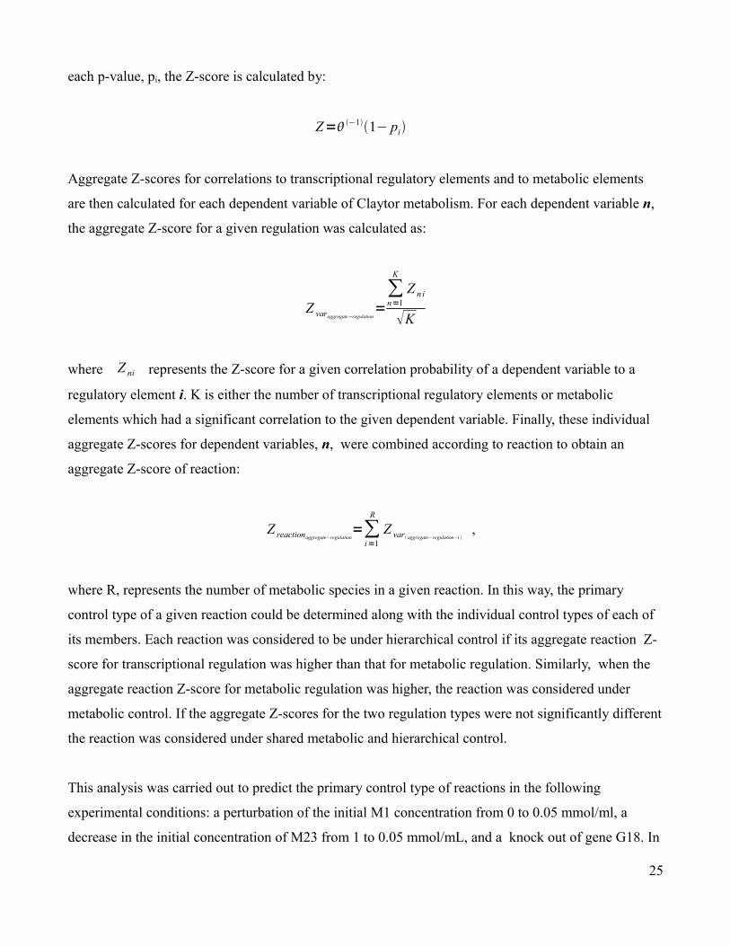
each p-value, pi, the Z-score is calculated by:

Z= −11− pi

Aggregate Z-scores for correlations to transcriptional regulatory elements and to metabolic elements

are then calculated for each dependent variable of Claytor metabolism. For each dependent variable n,

the aggregate Z-score for a given regulation was calculated as:

Z varaggregate−regulation=∑n=1

K

Z n i

K

where Z ni represents the Z-score for a given correlation probability of a dependent variable to a

regulatory element i. K is either the number of transcriptional regulatory elements or metabolic

elements which had a significant correlation to the given dependent variable. Finally, these individual

aggregate Z-scores for dependent variables, n, were combined according to reaction to obtain an

aggregate Z-score of reaction:

Z reactionaggregate−regulation=∑

i=1

R

Z var aggregate−regulation−i ,

where R, represents the number of metabolic species in a given reaction. In this way, the primary

control type of a given reaction could be determined along with the individual control types of each of

its members. Each reaction was considered to be under hierarchical control if its aggregate reaction Z-

score for transcriptional regulation was higher than that for metabolic regulation. Similarly, when the

aggregate reaction Z-score for metabolic regulation was higher, the reaction was considered under

metabolic control. If the aggregate Z-scores for the two regulation types were not significantly different

the reaction was considered under shared metabolic and hierarchical control.

This analysis was carried out to predict the primary control type of reactions in the following

experimental conditions: a perturbation of the initial M1 concentration from 0 to 0.05 mmol/ml, a

decrease in the initial concentration of M23 from 1 to 0.05 mmol/mL, and a knock out of gene G18. In

25

each case, a time course ranging from 0 to 500 model time units was simulated and measurements were

sampled at every 50th interval.

In some cases, a given experiment can provide no information concerning the control of a given

dependent variable. For example, this can occur in perturbations where there is no effect upon a

variable's concentration. When the concentration of a variable does not change, calculations of its

Kendall's correlation with other variables is impossible. In these cases, the variable is excluded.

It is important to note that this procedure is significantly different than metabolic control analysis

(Kacser & JA Burns 1995; Kacser & J. A. Burns 1979; Heinrich & Schuster 1996) or hierarchical

control analysis (HCA) (H.V. Westerhoff & Kahn 1993; ter Kuile & H. V. Westerhoff 2001; A de la

Fuente et al. 2002) and gives a different type of result. The prediction made here is based upon how

correlated the dependent variables of metabolism (those which are substrates and products of metabolic

reactions) are with moieties that are associated with a given form of control. These correlations can

differ depending upon the experimental condition. The goal of this analysis is to determine if high

levels of correlation with these purported regulatory elements makes it possible to predict how likely it

is to get close to the true system parameters under certain experimental conditions by only examining

metabolism.

Determining Model Performance

The ability of a given model to accurately describe the system level properties of the Claytor network

was determined in two ways. As a first measure, the sum of squares between a given model and the

data was used. In particular, the sum of squares of the overall fit of the model to the data as well as that

of the individual fits to the pertinent dependent variables were taken into account.

As a second measure, a visual assessment of the fit of the dependent variables of interest to the data

was taken. The dependent values of interest in this case were the metabolites and the proteins which

played a direct role, as opposed to a modifying role, in the metabolic reactions. The quality fit of each

dependent variable was visually graded using a binary scheme. Each fit was assigned a bit string based

on an assessment of certain features. These features and the criteria for each one to be defined as either

26

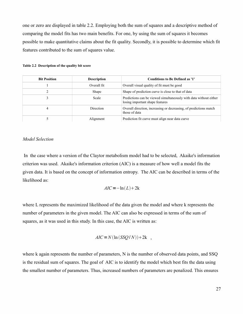
one or zero are displayed in table 2.2. Employing both the sum of squares and a descriptive method of

comparing the model fits has two main benefits. For one, by using the sum of squares it becomes

possible to make quantitative claims about the fit quality. Secondly, it is possible to determine which fit

features contributed to the sum of squares value.

Table 2.2 Description of the quality bit score

Bit Position Description Conditions to Be Defined as '1'

1 Overall fit Overall visual quality of fit must be good

2 Shape Shape of prediction curve is close to that of data

3 Scale Predictions can be viewed simultaneously with data without either losing important shape features

4 Direction Overall direction, increasing or decreasing, of predictions match those of data

5 Alignment Prediction fit curve must align near data curve

Model Selection

In the case where a version of the Claytor metabolism model had to be selected, Akaike's information

criterion was used. Akaike's information criterion (AIC) is a measure of how well a model fits the

given data. It is based on the concept of information entropy. The AIC can be described in terms of the

likelihood as:

AIC=−lnL2k

where L represents the maximized likelihood of the data given the model and where k represents the

number of parameters in the given model. The AIC can also be expressed in terms of the sum of

squares, as it was used in this study. In this case, the AIC is written as:

AIC=N ln SSQ /N 2k ,

where k again represents the number of parameters, N is the number of observed data points, and SSQ

is the residual sum of squares. The goal of AIC is to identify the model which best fits the data using

the smallest number of parameters. Thus, increased numbers of parameters are penalized. This ensures

27

that a model will not be selected simply because it fits the dataset perfectly as there is some preference

for simpler models. In cases where the AIC values of differing models were compared, the one with

the smallest AIC was selected (Akaike 1974; Burnham & Anderson 1998).

Results and Discussion

Determining the Subset of Reactions to be Included in the Metabolism Model

It is a common practice in many systems biology studies for the metabolome, the genome, and the

transcriptome to be studied separately. In order to determine the effect of analyzing the metabolome in

isolation, the metabolism portion of the Claytor network was extracted from the full network and

parametrized as described in the experimental design section . As mentioned in the experimental

design section on forming the Claytor metabolism model using the original kinetics, a decision had to

be made whether to include the signaling reactions for M1 and M3. While all of the other metabolic

reactions are primarily composed of metabolites, proteins play a primary role in the M1 and M3

signaling reactions. In these reactions, the signaling metabolite, M1 or M3, interacts with a receptor

protein to form a transcription factor. This transcription factor subsequently activates a cascade of

transcriptional-mediated events which compensate for the presence of the signaling metabolites.

Because the metabolites act as part of a signaling cascade in these reactions, it was unclear if they

should be included in the metabolism models. In order to solve this dilemma, two Claytor metabolism

models were constructed and their respective parameters estimated. In one model, the M1 and M3

signaling reactions were included, while in the other they were not. The two models were compared

using the Akaike's information criterion (AIC). The results of this comparison are shown in table 2.3.

The model which excluded the M1 and M3 signaling reactions obtained the lowest AIC value.

Therefore, this model was chosen to represent the metabolic portion of the Claytor network both here

and in the later metabolism models where the true rate equations are replaced with estimated versions.

Table 2.3 : A comparison of two different versions of the metabolism model considered

Metabolism Model Number of Parameters Number of Data Points Sum of Squares AIC

Including M1 and M3 33 7280 1.10E-04 3.49E+05

28

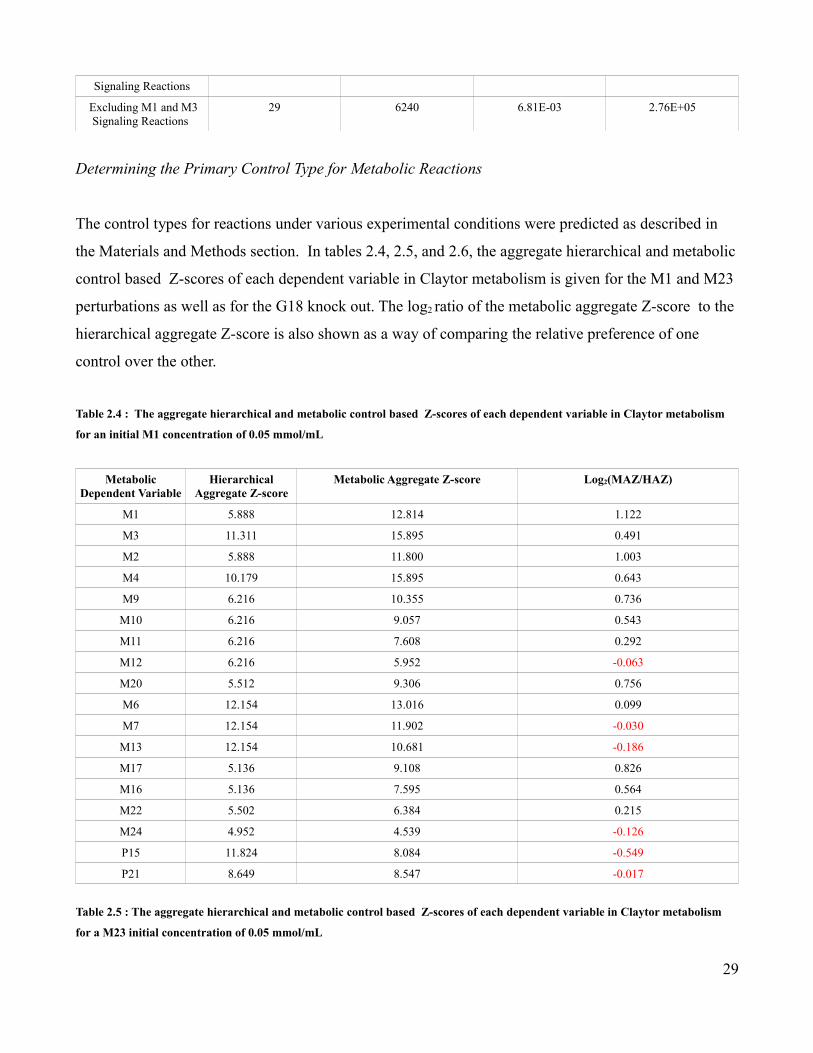
Signaling Reactions

Excluding M1 and M3 Signaling Reactions

29 6240 6.81E-03 2.76E+05

Determining the Primary Control Type for Metabolic Reactions

The control types for reactions under various experimental conditions were predicted as described in

the Materials and Methods section. In tables 2.4, 2.5, and 2.6, the aggregate hierarchical and metabolic

control based Z-scores of each dependent variable in Claytor metabolism is given for the M1 and M23

perturbations as well as for the G18 knock out. The log2 ratio of the metabolic aggregate Z-score to the

hierarchical aggregate Z-score is also shown as a way of comparing the relative preference of one

control over the other.

Table 2.4 : The aggregate hierarchical and metabolic control based Z-scores of each dependent variable in Claytor metabolism

for an initial M1 concentration of 0.05 mmol/mL

Metabolic Dependent Variable

Hierarchical Aggregate Z-score

Metabolic Aggregate Z-score Log2(MAZ/HAZ)

M1 5.888 12.814 1.122

M3 11.311 15.895 0.491

M2 5.888 11.800 1.003

M4 10.179 15.895 0.643

M9 6.216 10.355 0.736

M10 6.216 9.057 0.543

M11 6.216 7.608 0.292

M12 6.216 5.952 -0.063

M20 5.512 9.306 0.756

M6 12.154 13.016 0.099

M7 12.154 11.902 -0.030

M13 12.154 10.681 -0.186

M17 5.136 9.108 0.826

M16 5.136 7.595 0.564

M22 5.502 6.384 0.215

M24 4.952 4.539 -0.126

P15 11.824 8.084 -0.549

P21 8.649 8.547 -0.017


for a M23 initial concentration of 0.05 mmol/mL

29




M1 No Information No Information No Information

M3 2.950 13.522 2.197


M4 3.909 13.095 1.744

M9 4.194 13.041 1.637

M10 4.194 12.075 1.526

M11 4.194 11.054 1.398

M12 3.648 9.549 1.388

M20 2.328 9.720 2.062

M6 4.328 11.689 1.433

M7 5.012 11.043 1.140

M13 6.104 5.626 -0.118

M17 2.328 10.975 2.237

M16 2.328 12.123 2.381

M22 2.328 8.324 1.838

M24 2.328 6.737 1.533

P15 5.326 8.122 0.609

P21 5.326 6.418 0.269


for a G18 knock out





M3 6.551 12.704 0.955


M4 3.870 10.024 1.373




M12 2.467 3.901 0.661


M6 7.770 10.685 0.460

M7 8.081 9.046 0.163

M13 8.647 6.884 -0.329

M17 4.739 6.900 0.542

M16 7.810 5.548 -0.493


30


P15 No Information No Information No Information

P21 No Information No Information No Information

As can be seen in table, many of the aggregate Z-scores for the dependent variables show a preference

for metabolic control in all of the experimental conditions under study. In the M1 perturbation

experiment, 12 of 18 variables showing at least a weak preference. In the perturbation of the

concentration of M23, all but one variable, M13, has a higher metabolic aggregate Z-score value than a

hierarchical one. The metabolic aggregate Z-scores for this experiment are much higher than in the

M1 perturbation.

No control preference could be assigned to M1 or M2 in this case, as neither dependent variable's

concentration was affected by the M23 perturbation. This result is to be expected, as M1 is a toxic

element and M2 is involved with its removal. Unless M1 is directly perturbed, these concentrations are

unlikely to change. The knock out of G18 affected the least number of metabolic dependent variables,

resulting in information for only 8 of the 18 total variables. This phenomenon is paralleled in other

biological studies. Certain experimental perturbations will yield more information than others and care

must be taken to account for this. In this case, the more information rich dataset, the M1 perturbation,

is used to estimate the model parameters. If one of the less information rich datasets had been used, it is

unlikely that the resultant model would be able to account for changes associated with an M1

perturbation.

Of the three experiments, the M1 perturbation contains the highest number of dependent variables with

stronger hierarchical associated control aggregate Z-scores. However, many of the log2 ratios of these

are close to 0, and therefore cannot be confidently classified as under transcriptional control. In all

three experiments, metabolite M13 was unique in that it consistently had a higher aggregate Z-score for

hierarchical control than for metabolic control.

For each reaction, the substrate and reactant aggregate Z-scores are summed for each control type, as

mentioned in the materials and methods section. These reaction sums of the aggregate Z-scores for

each control type and experimental condition are shown below in tables 2.7, 2.8, and 2.9 along with

31

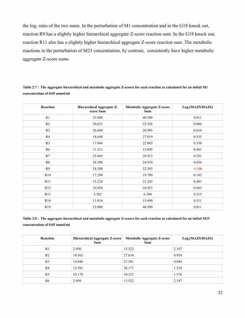
the log2 ratio of the two sums. In the perturbation of M1 concentration and in the G18 knock out,

reaction R9 has a slightly higher hierarchical aggregate Z-score reaction sum. In the G18 knock out,

reaction R11 also has a slightly higher hierarchical aggregate Z-score reaction sum .The metabolic

reactions in the perturbation of M23 concentration, by contrast, consistently have higher metabolic

aggregate Z-score sums.

Table 2.7 : The aggregate hierarchical and metabolic aggregate Z-scores for each reaction as calculated for an initial M1

concentration of 0.05 mmol/ml

Reaction Hierarchical Aggregate Z-score Sum

Metabolic Aggregate Z-score Sum

Log2(MAZS/HAZS)

R1 23.088 40.509 0.811

R2 30.651 32.526 0.086

R3 26.689 26.985 0.016

R4 18.648 27.019 0.535

R5 17.944 22.865 0.350

R6 11.311 15.895 0.491

R7 23.465 28.912 0.301

R8 24.308 24.919 0.036

R9 24.308 22.583 -0.106

R10 17.290 19.789 0.195

R11 15.224 21.243 0.481

R12 10.454 10.923 0.063

R13 5.502 6.384 0.215

R14 11.014 15.690 0.511

R19 23.088 40.509 0.811

Table 2.8 : The aggregate hierarchical and metabolic aggregate Z-scores for each reaction as calculated for an initial M23

concentration of 0.05 mmol/ml



Log2(MAZS/HAZS)

R1 2.950 13.522 2.197

R2 14.562 27.634 0.924

R3 14.846 27.581 0.894

R4 12.581 36.171 1.524

R5 10.170 30.323 1.576

R6 2.950 13.522 2.197

32

R7 7.277 25.211 1.793

R8 9.340 22.732 1.283

R9 11.116 16.669 0.585

R10 8.433 16.602 0.977

R11 6.985 29.835 2.095

R12 4.657 15.061 1.693

R13 2.328 8.324 1.838

R14 4.657 18.044 1.954

R19 2.950 13.522 2.197

Table 2.9 : The aggregate hierarchical and metabolic aggregate Z-scores for each reaction as calculated for a knockout of G18



Log2(MAZS/HAZS)

R1 6.551 12.704 0.955

R2 3.870 10.024 1.373

R3 No Information No Information No Information


R5 2.467 3.901 0.661

R6 6.551 12.704 0.955

R7 14.321 23.390 0.708

R8 15.851 19.731 0.316

R9 16.728 15.929 -0.071

R10 13.386 13.784 0.042

R11 12.549 12.449 -0.012




R19 6.551 12.704 0.955

Based upon these results, it is predicted that using an isolated model of metabolism to study these

reactions would be appropriate and that regulation by transcription/translation and signaling were

minor effects in the data. Because most of the dependent variables of metabolism under study as well

as their reactions are more associated with metabolic control elements, excluding transcriptional

control should not significantly negatively impact the study. In cases where a given dependent variable

has difficulty being fit in a certain perturbation, it is expected that it will have a higher hierarchical

control based aggregate Z-score or only a slightly higher metabolic one. It is further predicted that

those reactions which have the lowest metabolic control based aggregate Z-score sums will achieve

33

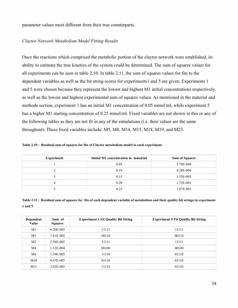
parameter values most different from their true counterparts.

Claytor Network Metabolism Model Fitting Results

Once the reactions which comprised the metabolic portion of the claytor network were established, its

ability to estimate the true kinetics of the system could be determined. The sum of squares values for

all experiments can be seen in table 2.10. In table 2.11, the sum of squares values for fits to the

dependent variables as well as the bit string scores for experiments1 and 5 are given. Experiments 1

and 5 were chosen because they represent the lowest and highest M1 initial concentrations respectively,

as well as the lowest and highest experimental sum of squares values. As mentioned in the material and

methods section, experiment 1 has an initial M1 concentration of 0.05 mmol/ml, while experiment 5

has a higher M1 starting concentration of 0.25 mmol/ml. Fixed variables are not shown in this or any of

the following tables as they are not fit in any of the simulations (i.e. their values are the same

throughout). These fixed variables include: M5, M8, M14, M15, M18, M19, and M23.

Table 2.10 : Residual sum of squares for fits of Claytor metabolism model to each experiment

Experiment Initial M1 concentration in mmol/ml Sum of Squares

1 0.05 5.78E-004

2 0.10 9.28E-004

3 0.15 1.35E-003

4 0.20 1.72E-003

5 0.25 1.87E-003

Table 2.11 : Residual sum of squares for fits of each dependent variable of metabolism and their quality bit strings in experiment

1 and 5

Dependent Value

Sum of Squares

Experiment 1 Fit Quality Bit String Experiment 5 Fit Quality Bit String

M1 6.20E-005 11111 11111

M3 7.61E-005 00110 00110

M2 2.58E-005 11111 11111

M4 1.32E-004 00100 00100

M9 1.39E-005 11110 01110

M10 8.67E-005 01110 01110

M11 3.02E-005 11110 01110

34

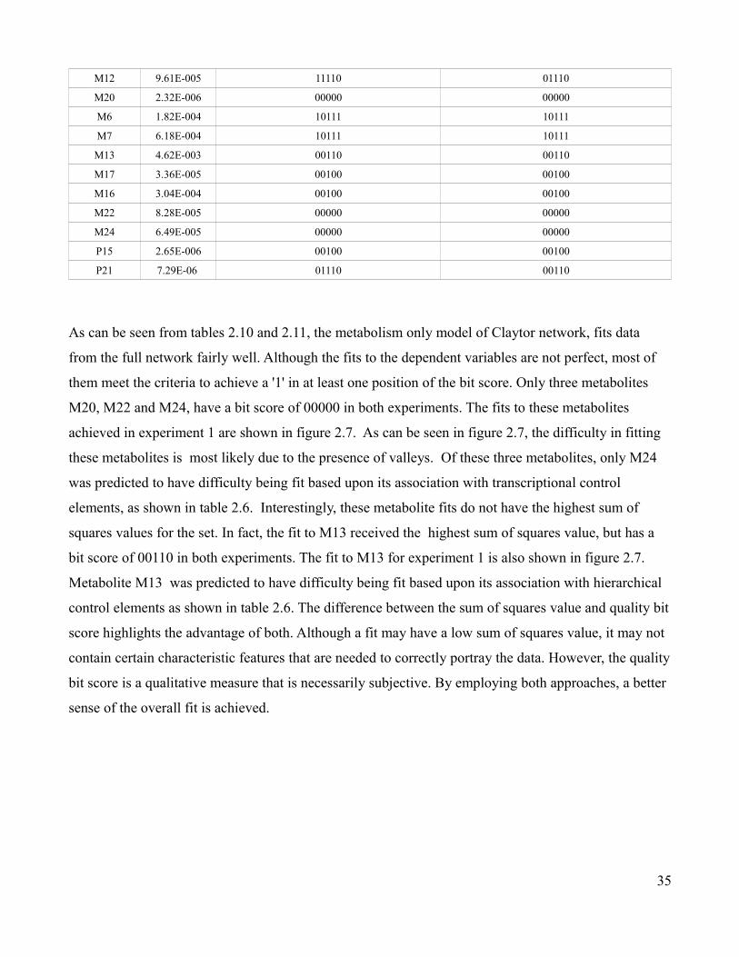
M12 9.61E-005 11110 01110

M20 2.32E-006 00000 00000

M6 1.82E-004 10111 10111

M7 6.18E-004 10111 10111

M13 4.62E-003 00110 00110

M17 3.36E-005 00100 00100

M16 3.04E-004 00100 00100

M22 8.28E-005 00000 00000

M24 6.49E-005 00000 00000

P15 2.65E-006 00100 00100

P21 7.29E-06 01110 00110

As can be seen from tables 2.10 and 2.11, the metabolism only model of Claytor network, fits data

from the full network fairly well. Although the fits to the dependent variables are not perfect, most of

them meet the criteria to achieve a '1' in at least one position of the bit score. Only three metabolites

M20, M22 and M24, have a bit score of 00000 in both experiments. The fits to these metabolites

achieved in experiment 1 are shown in figure 2.7. As can be seen in figure 2.7, the difficulty in fitting

these metabolites is most likely due to the presence of valleys. Of these three metabolites, only M24

was predicted to have difficulty being fit based upon its association with transcriptional control

elements, as shown in table 2.6. Interestingly, these metabolite fits do not have the highest sum of

squares values for the set. In fact, the fit to M13 received the highest sum of squares value, but has a

bit score of 00110 in both experiments. The fit to M13 for experiment 1 is also shown in figure 2.7.

Metabolite M13 was predicted to have difficulty being fit based upon its association with hierarchical

control elements as shown in table 2.6. The difference between the sum of squares value and quality bit

score highlights the advantage of both. Although a fit may have a low sum of squares value, it may not

contain certain characteristic features that are needed to correctly portray the data. However, the quality

bit score is a qualitative measure that is necessarily subjective. By employing both approaches, a better

sense of the overall fit is achieved.

35

A.

B.

C.

36

Change in M20 Over Time

0.50375

0.5038

0.50385

0.5039

0.50395

0.504

0.50405

0 30 60 90 120

150

180

210

240

270

300

T im e

Conc

entra

tion

in m

mol

/mL

M20_measured


2.0988

2.099

2.0992

2.0994

2.0996

2.0998

2.1

2.1002

0 30 60 90 120

150

180

210

240

270

300

Tim e

Conc

entra

tion

in m

mol

/mL

M22_measured

M22 Fitting Result

2.06

2.08

2.1

2.12

2.14

2.16

2.18

0 30 60 90 120

150

180

210

240

270

300

T im e

Conc

entra

tion

in m

mol

/mL

M22_measuredM22_fitted_value


4.82654.827

4.82754.828

4.82854.829

4.82954.83

4.8305

0 30 60 90 120

150

180

210

240

270

300

Tim e

Conc

entra

tion

in m

mol

/mL

M24_measured

M24 Fitting Results

4.784.8

4.824.844.864.884.9

4.924.94

0 30 60 90 120

150

180

210

240

270

300

T im e

Conc

entra

tion

in m

mol

/mL


M20 Fitting Result

0.5010.5020.5030.5040.5050.5060.5070.5080.5090.51

0 30 60 90 120

150

180

210

240

270

300

T im e

Conc

enta

rtion

in m

mol

/mL


D.

Figure 2.7. The dependent variables which received the lowest quality bit score are shown along with the metabolite which received the

largest sum of squares value. Displayed are the results from experiment 1. A. A plot of the concentration of metabolite M20 is shown in

isolation and with its fitted value. B. A plot of the concentration of metabolite M22 is shown in isolation and with its fitted value. C. A

plot of the concentration of metabolite M24 is shown in isolation and with its fitted value. D. A plot of the fit to the concentration of

M13 .

While both experiments resulted in identical quality bit scores for many of the dependent variables,

there were some instances where they differed. In the dependent variables M9, M10, M11, M17, and

P21, the fits received different quality scores in each experiment. In all of these cases, the fit to

experiment 1 has a better quality bit score than in experiment 5. Most of the differences between the

quality bit scores was in the category of “Overall Fit”. This difference occurred in fits to the metabolic

concentrations of M9, M10, and M11. In figure 2.9, a plot of the measured M9 concentrations in both

experiments and their respective fits in these two experiments is given. The quality bit scores also

differed between experiments in the category of “Shape” for P21. Plots of the fits to these metabolites

and protein for each experiment are also given in figure 2.9.

37

M13 Fitting Result

0

0.5

1

1.5

2

2.5

3

0 30 60 90 120

150

180

210

240

270

300

Tim e

Conc

entra

tion

in m

mol

/mL


A.

B.

Figure 2.8. A comparison between the fits in experiments 1 and 5 for M9 and P21. A. The difference in overall quality of fit is depicted

for M9, with the best fit being achieved for experiment 1. B. A simultaneous plot of the fitted and measured values of P21 in experiments

1 and 5 is shown on the left . On the right, the fitted values for P21 are shown in isolation from the measured values in order to

demonstrate that the fit to P21 in experiment 1 has the same overall shape as its measured value. Although the fit to P21 in experiment 5

has a similar shape, it was not adequate to receive a quality bit score of 1 in this category.

The top three dependent variables of metabolism which were predicted to be most likely to have

difficulty being fit were P15, M13, and M24. Metabolite M13 received the highest sum of squares

value, but not the lowest quality bit score. Metabolite M24, by contrast, had a low sum of squares value

by comparison, but had one of the lowest quality bit scores. Protein P15 had a low quality bit score but

also a low sum of squares value. Of the remaining dependent variables which were predicted to have

38

Comparison of Fits to M9

0

0.01

0.02

0.03

0.04

0.05

0.06

0.07

0 30 60 90 120

150

180

210

240

270

300

Time

Con

cent

ratio

n in

mm

ol/m

L

M9_exp1_measuredM9_exp5_measuredM9_exp5_fittedM9_exp1_fitted

P21 Fitted Values

0.00E+00

5.00E-05

1.00E-04

1.50E-04

2.00E-04

2.50E-04

3.00E-040 30 60 90 120

150

180

210

240

270

300

Tim e

Conc

entra

tion

in m

mol

/mL

P21_exp1_fittedP21_exp5_fitted

Comparison of Fits to P21

0.00E+002.00E-044.00E-046.00E-048.00E-041.00E-031.20E-031.40E-031.60E-031.80E-03

0 30 60 90 120

150

180

210

240

270

300

Time

Con

cent

ratio

n in

mm

ol/m

L

P21_exp1_measuredP21_exp1_fittedP21_exp5_measuredP21_exp5_fitted

fitting difficulty, M6 , M7 , and M12 received some of the highest sum of squares values, yet had

acceptable quality bit scores. Protein P21 had a low sum of squares value and an acceptable quality bit

score. Certain metabolites which were not fit well, M22 , M20 and M16 for example, were not

predicted as having difficulty via the control association method. Therefore, while a metabolite's

correlation with control elements seems to have some effect on it's ability to be fit, it is not the only

factor.

Claytor Metabolism Model Applied to New Perturbations

After the Claytor metabolic model was parametrized by being fit to the M1 perturbation and G16 knock

out datasets as described above, its ability to accurately describe new experimental conditions was

tested. In tables 2.12 and 2.12, the sum of squares values for results of the fits of the model to

perturbations in the concentration of M23 along with their respective quality bit scores is given.

Metabolite M13 was predicted by the control association method to have difficulty being fit in the

current experiment. This prediction is verified in this case, as M13 has one of the lowest quality bit

scores and the highest sum of squares values. However, other badly fit dependent variables present

were not predicted via the control association method. In particular, M4 which received the lowest

quality bit score, was not targeted by the method. Its fitting difficulty is most likely perpetuated from

the low quality fit that was achieved to the M1 perturbation dataset which was used to determine the

parameter values for the model.

Table 2.12 : Results of the dependent variable fits to different perturbations of the concentration of M23


1 0.05 7.72E-05

2 0.44 1.65E-04

3 0.83 1.65E-04

4 1.22 1.64E-04

5 1.61 1.64E-04

6 2.00 1.63E-04

Table 2.13 : Residual sum of squares values and quality bit scores assigned to each dependent variable in experiments 1 and 3

39

Dependent Value

Sum of Squares


M1 5.20E-49 11111 11111

M3 1.38E-05 00010 00010

M2 5.20E-49 11111 11111

M4 6.53E-08 00000 00000

M9 3.05E-08 01110 01110

M10 4.80E-08 01110 01110

M11 3.34E-08 01110 01110

M12 4.10E-08 01110 01110

M20 5.48E-10 11111 11111

M6 2.76E-05 00010 00010

M7 1.10E-04 00010 00010

M13 7.46E-04 00010 00010

M17 9.29E-08 01110 01110

M16 9.88E-08 01110 01110

M22 1.99E-08 11111 11111

M24 1.55E-08 11111 11111

P15 4.42E-11 01010 01010

P21 5.51E-10 01010 01010

The fit results of the Claytor metabolism model fits to the G18 knock out experiment are shown in

tables 2.14 and 2.15. In this experiment, metabolites M13 and M16 were predicted as being hard to fit .

The results in table 2.15 agree with these predictions. However, many other dependent variables also

had low quality bit scores in this experiment, although their sum of squares values are low. Similar to

the M23 perturbation, some of the depend variables have difficulty achieving high quality bit scores

because they did not do so in the M1 dataset. Although the Claytor metabolism model did not perform

well using the qualitative measure of fit represented as the quality bit score, the sum of squares values

for fits to the variables is very good. This seems to indicate that although the Claytor metabolism model

may miss certain qualitative features of the perturbation, in most cases it predicts a value which is very

close to the true one.

Table 2.14 : Residual sum of squares for the fit of the Claytor metabolism model to the G18 knock out experiment

Experiment Sum of Squares

G18 Knock Out 0.000164982

40

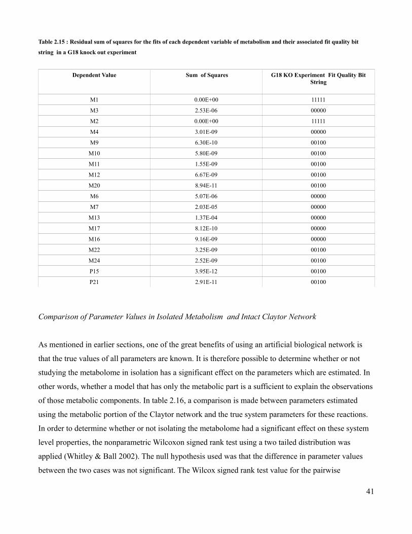
Table 2.15 : Residual sum of squares for the fits of each dependent variable of metabolism and their associated fit quality bit

string in a G18 knock out experiment

Dependent Value Sum of Squares G18 KO Experiment Fit Quality Bit String

M1 0.00E+00 11111

M3 2.53E-06 00000

M2 0.00E+00 11111

M4 3.01E-09 00000

M9 6.30E-10 00100

M10 5.80E-09 00100

M11 1.55E-09 00100

M12 6.67E-09 00100

M20 8.94E-11 00100

M6 5.07E-06 00000

M7 2.03E-05 00000

M13 1.37E-04 00000

M17 8.12E-10 00000

M16 9.16E-09 00000

M22 3.25E-09 00100

M24 2.52E-09 00100

P15 3.95E-12 00100

P21 2.91E-11 00100

Comparison of Parameter Values in Isolated Metabolism and Intact Claytor Network

As mentioned in earlier sections, one of the great benefits of using an artificial biological network is

that the true values of all parameters are known. It is therefore possible to determine whether or not

studying the metabolome in isolation has a significant effect on the parameters which are estimated. In

other words, whether a model that has only the metabolic part is a sufficient to explain the observations

of those metabolic components. In table 2.16, a comparison is made between parameters estimated

using the metabolic portion of the Claytor network and the true system parameters for these reactions.

In order to determine whether or not isolating the metabolome had a significant effect on these system

level properties, the nonparametric Wilcoxon signed rank test using a two tailed distribution was

applied (Whitley & Ball 2002). The null hypothesis used was that the difference in parameter values

between the two cases was not significant. The Wilcox signed rank test value for the pairwise

41

comparison between all parameters in the metabolic portion of the Claytor network was W = 2119, with

a p-value of P = 0.007997. These results indicate that there is a significant overall difference between

the parameter values of the isolated and the intact Claytor metabolic networks. By contrast, when

comparisons are made between the parameters in individual reactions, these differences are no longer

significant at the α = 0.05 level, as shown in table 2.16. This is to be expected as the number of

samples being tested is much smaller. When each reaction is tested individually, multiple testing must

be taken into account. After the Bonferroni correction (Weir 1996) is applied, the new significance

level required is β = .0033. The reaction which is closest to being significantly different between the

isolated metabolic and full Claytor networks is R11, which has a Wilcoxon p-value of P=0.0625.

However, even this reaction is far from the acceptable significance level employed. The least

significant p-values were obtained for reactions R1 and R2. While the difference in the quality of fits

achieved by members in each reaction could in part explain this difference, it does not explain it fully.

While reactions R1 and R2 contain some of the dependent variables which were fit the best, according

to their quality bit score, R19 also contains these well fit metabolites. Similarly, R11 contains the fixed

metabolite M19 and several metabolites which did not receive very high quality bit scores. However,

except for M19, these metabolites are present in other reactions. While M19 is not shared, other fixed

metabolites are present in reactions which received much higher p-values. For example, R10 which has

a Wilcoxon p-value of P = 0.8438, contains M16 and M17. Metabolite M24 is also shared with

reaction R12, which has a Wilcoxon p-value of P = 0.625. Therefore, it is unlikely that any one

metabolite fit, or misfit, is responsible for the lower R11 p-value.

According to the reaction sums of the control associated aggregate Z-scores for the M1 perturbation

experiment , reactions R3, R8, and R9 were predicted as having the parameters which were the most

different from the true values. Reaction R9 is predicted as having the largest difference between its

predicted parameters and the true ones. These predictions are not verified by the results in table 2.16 .

The G18 knock out experiment also predicted difficulty in obtaining good parameter estimates for

reaction R9 as well as for R10 and R11. Although reaction R11 has the smallest Wilcoxon p-value, it as

well as the p-values for reactions R9 and R10 are far from being significant.

Table 2.16 : Comparison of the true kinetic parameters of the Claytor network with those estimated using only the metabolic

reactions

42

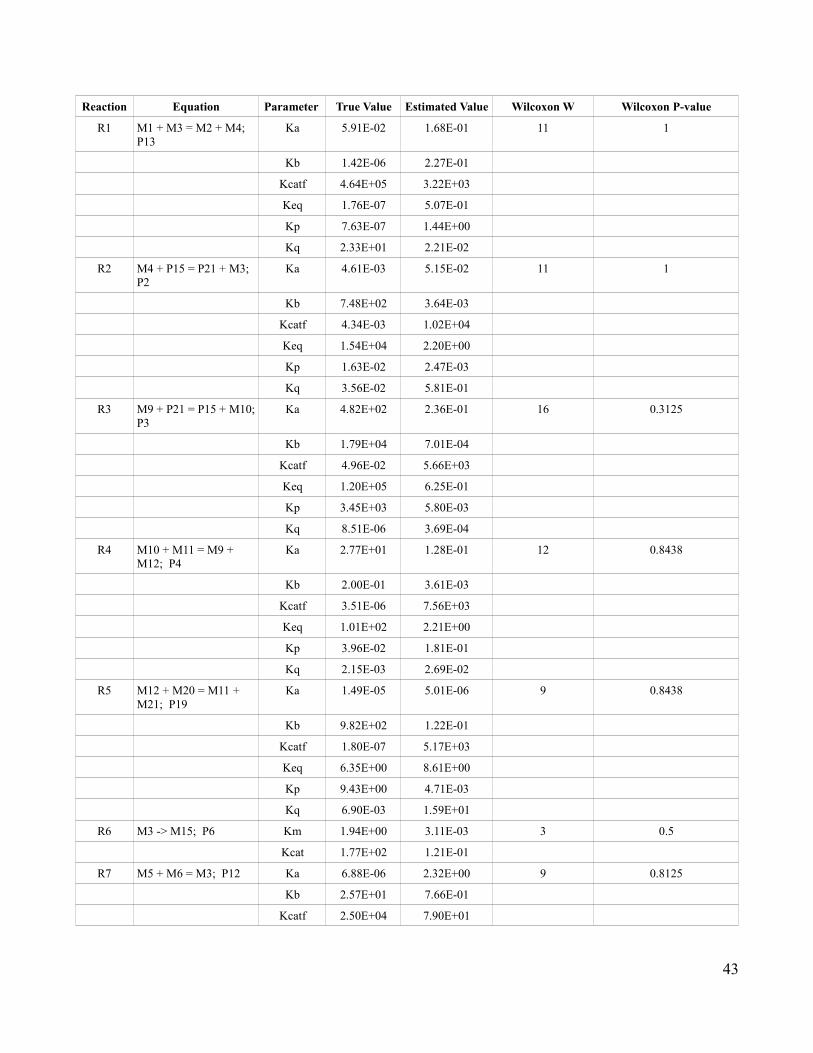
Reaction Equation Parameter True Value Estimated Value Wilcoxon W Wilcoxon P-value

R1 M1 + M3 = M2 + M4; P13

Ka 5.91E-02 1.68E-01 11 1

Kb 1.42E-06 2.27E-01

Kcatf 4.64E+05 3.22E+03

Keq 1.76E-07 5.07E-01

Kp 7.63E-07 1.44E+00

Kq 2.33E+01 2.21E-02

R2 M4 + P15 = P21 + M3; P2

Ka 4.61E-03 5.15E-02 11 1

Kb 7.48E+02 3.64E-03

Kcatf 4.34E-03 1.02E+04

Keq 1.54E+04 2.20E+00

Kp 1.63E-02 2.47E-03

Kq 3.56E-02 5.81E-01

R3 M9 + P21 = P15 + M10; P3

Ka 4.82E+02 2.36E-01 16 0.3125

Kb 1.79E+04 7.01E-04

Kcatf 4.96E-02 5.66E+03

Keq 1.20E+05 6.25E-01

Kp 3.45E+03 5.80E-03

Kq 8.51E-06 3.69E-04

R4 M10 + M11 = M9 + M12; P4

Ka 2.77E+01 1.28E-01 12 0.8438

Kb 2.00E-01 3.61E-03

Kcatf 3.51E-06 7.56E+03

Keq 1.01E+02 2.21E+00

Kp 3.96E-02 1.81E-01

Kq 2.15E-03 2.69E-02

R5 M12 + M20 = M11 + M21; P19

Ka 1.49E-05 5.01E-06 9 0.8438

Kb 9.82E+02 1.22E-01

Kcatf 1.80E-07 5.17E+03

Keq 6.35E+00 8.61E+00

Kp 9.43E+00 4.71E-03

Kq 6.90E-03 1.59E+01

R6 M3 -> M15; P6 Km 1.94E+00 3.11E-03 3 0.5

Kcat 1.77E+02 1.21E-01

R7 M5 + M6 = M3; P12 Ka 6.88E-06 2.32E+00 9 0.8125

Kb 2.57E+01 7.66E-01

Kcatf 2.50E+04 7.90E+01

43

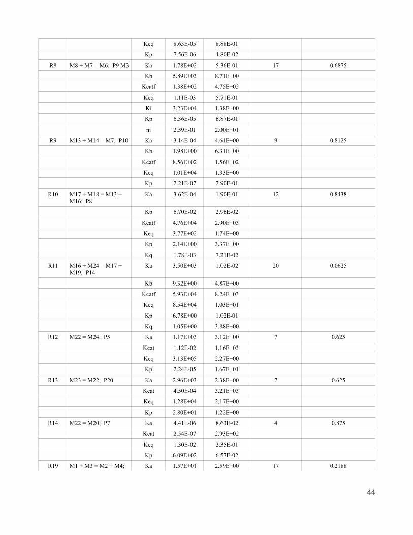
Keq 8.63E-05 8.88E-01

Kp 7.56E-06 4.80E-02

R8 M8 + M7 = M6; P9 M3 Ka 1.78E+02 5.36E-01 17 0.6875

Kb 5.89E+03 8.71E+00

Kcatf 1.38E+02 4.75E+02

Keq 1.11E-03 5.71E-01

Ki 3.23E+04 1.38E+00

Kp 6.36E-05 6.87E-01

ni 2.59E-01 2.00E+01

R9 M13 + M14 = M7; P10 Ka 3.14E-04 4.61E+00 9 0.8125

Kb 1.98E+00 6.31E+00

Kcatf 8.56E+02 1.56E+02

Keq 1.01E+04 1.33E+00

Kp 2.21E-07 2.90E-01

R10 M17 + M18 = M13 + M16; P8

Ka 3.62E-04 1.90E-01 12 0.8438

Kb 6.70E-02 2.96E-02

Kcatf 4.76E+04 2.90E+03

Keq 3.77E+02 1.74E+00

Kp 2.14E+00 3.37E+00

Kq 1.78E-03 7.21E-02

R11 M16 + M24 = M17 + M19; P14

Ka 3.50E+03 1.02E-02 20 0.0625

Kb 9.32E+00 4.87E+00

Kcatf 5.93E+04 8.24E+03

Keq 8.54E+04 1.03E+01

Kp 6.78E+00 1.02E-01

Kq 1.05E+00 3.88E+00

R12 M22 = M24; P5 Ka 1.17E+03 3.12E+00 7 0.625

Kcat 1.12E-02 1.16E+03

Keq 3.13E+05 2.27E+00

Kp 2.24E-05 1.67E+01

R13 M23 = M22; P20 Ka 2.96E+03 2.38E+00 7 0.625

Kcat 4.50E-04 3.21E+03

Keq 1.28E+04 2.17E+00

Kp 2.80E+01 1.22E+00

R14 M22 = M20; P7 Ka 4.41E-06 8.63E-02 4 0.875

Kcat 2.54E-07 2.93E+02

Keq 1.30E-02 2.35E-01

Kp 6.09E+02 6.57E-02

R19 M1 + M3 = M2 + M4; Ka 1.57E+01 2.59E+00 17 0.2188

44

P16

Kb 2.50E+01 1.44E-01

Kcatf 2.78E+01 9.25E+00

Keq 6.31E+00 1.27E+01

Kp 7.65E+00 1.87E+00

Kq 2.90E-06 1.07E-02

Conclusions

It is common practice to make systems level predictions using only one aspect of the full biological

network, commonly the transcriptome or metabolome. This is due to both the technical difficulty

associated with obtaining data at more than one level as well as the difficulty in integrating the results

when multi-level experiments are done. Even under the most ideal circumstances, the true underlying

biological interaction network and the true system parameters are not known.

The goal of this study was to determine if there was an effect on the ability to assess system level

properties when the metabolic portion of the system is studied in isolation. By utilizing the Claytor

artificial biological network it was possible to characterize the effect that both incomplete network

knowledge as well as studying only the metabolic level had on this ability. It was hypothesized that the

elements which would be most negatively impacted would be those which were were most influenced

by transcription. The comparative influence of metabolic and transcriptional control was predicted by

using aggregate Z-scores for control association. These aggregate Z-scores were based upon the

correlation of the metabolically dependent variable in question and predetermined transcriptional and

metabolic control affiliated elements. It is important to note that correlation in metabolic systems can

be the result of factors which are not associated with control (Camacho et al. 2005). Therefore, it is

possible that the given method for predicting association with a control type may be an overestimation.

It is also likely that the influence of a given control type over a reaction is not purely the additive

contributions of its members. Therefore, there may be other more reliable indicators of transcriptional

influence.

The results of this study demonstrate that studying metabolism in isolation does affect the ability to

correctly estimate system parameters. Although association, as determined via aggregate Z-scores,

45

with hierarchical control did seem to influence this ability it is unlikely to be the sole factor. In

particular, it is likely that translational regulation, which was not assessed, also influences this ability.

46

Chapter 3: A Comparison of Generalized Kinetic Rate Laws

Background

Introduction

Enzyme kinetics play a critical role in forming dynamic models of biological systems . In order to be

able to simulate dynamics, it is not enough to merely know that an interaction or reaction occurs, it is

also necessary to know its rate of occurrence and how it depends on the concentration of the various

chemical species of the model – its kinetics, expressed through a mathematical function known as rate

law, rate function or kinetic function. Certain thermodynamic factors may make a given series of

reactions unfavorable or even impossible under cellular conditions. While rate laws for many enzymes

have been established by in vitro methods, there are still many enzymes for which appropriate kinetics

remain unknown. Although in vitro determined kinetics are useful for identifying the boundaries for

reactions, they may not always be the same as in the in vivo conditions (Teusink et al. 2000) . Enzyme

kinetic parameters are usually dependent on factors such as temperature and pH, and those are often

different in vitro from in vivo conditions. Unfortunately, no reliable method of determining in vivo

enzyme kinetic parameter values currently exists, making it difficult to determine whether most rate

functions determined in vitro have a correspondence to those occurring in the cell . However, even the

existence of such a method would not completely solve the problem. Enzymes, like other biochemical

moieties, behave differently depending on their tissue location and physiological condition (Steuer et

al. 2006), partly because of macromolecular crowding (Minton 2006) and other enzyme-enzyme

interactions (P. Mendes et al. 1992) . This lack of global, quantitative kinetic data combined with

observed inconsistencies in the in vivo data, has hindered the creation of network-scale kinetic models

of biochemical systems (Famili et al. 2005).

In order to compensate for this lack of available in vivo kinetic data, several methods for generalizing

rate laws have been proposed. The purpose of this study is to compare several of these methods using

the Claytor artificial biological network. These methods include: convenience (Liebermeister & Klipp

2006a; Liebermeister & Klipp 2006b), linlog (Visser & J. J. Heijnen 2003a) , and generalized mass

47

action kinetics (Guldberg & Waage 1879). In order to properly benchmark these differing methods, an

artificial biological network is used . The Claytor network , which was described in detail in chapter 2,

is ideal for these purposes as it contains many of the complex characteristics found in natural biological

systems while being much more tractable. In each case, the true values for the metabolic rate equation

are replaced with one of the generalized versions. In order to determine if some methods were more

sensitive to missing network information, two models were created to test each method. In one model,

the non-metabolic portion of Claytor network is left intact and in the other it is removed.

The Role of Kinetic functions in Forming Realistic Biological Models

It is important when modeling biological systems to take into account that the various chemical species

interact in a dynamic manner. The dynamics, or kinetics, of a given set of interactions affects both the

probability that the interaction will occur and what the impact of this interaction will be on the overall

system. Two methods which have been developed to account for the dynamic character of biological

systems are chemical kinetics and enzyme kinetics. In chemical kinetics, only the relationships between

products and reactants are considered . Chemical kinetics are portrayed using mass action kinetics

which was established by Guldberg and Waage (Guldberg & Waage 1879). Enzyme kinetics is based on

chemical kinetics and considers the effect of enzymes and also of modifiers (inhibitors, activators, etc.).

Mass action rate laws describe the kinetics of elementary reactions, whereas enzyme kinetic equations

employ a more macroscopic view, summarizing the behavior of all of the elementary reactions that

compose a full enzyme catalytic cycle. Both forms of kinetics can be useful for describing the

dynamics of biological systems depending on the assumptions that one is prepared to accept. The

following sections will focus on the properties of mass action and enzyme kinetics and briefly discuss

their use in biological studies.

Mass Action Kinetics

The law of mass action forms the basis of chemical kinetics (Klipp et al. 2005a). It emphasizes the

relationship between the rate of a reaction and the concentration of its components. Under mass action

kinetics, the rate of an elementary reaction is proportional to the probability of collisions of its

48

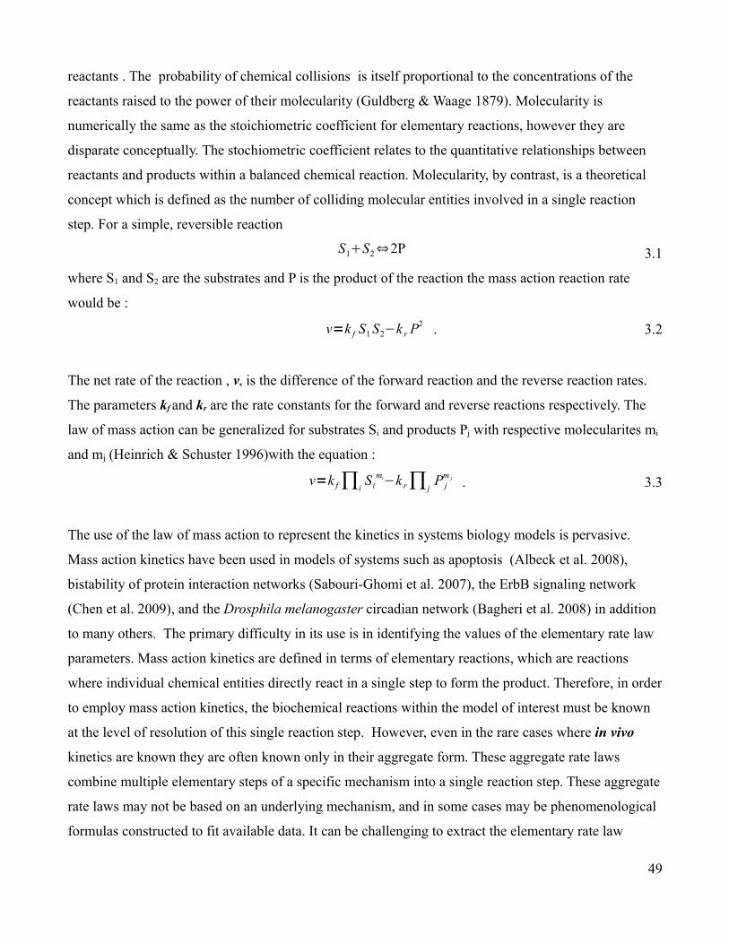
reactants . The probability of chemical collisions is itself proportional to the concentrations of the

reactants raised to the power of their molecularity (Guldberg & Waage 1879). Molecularity is

numerically the same as the stoichiometric coefficient for elementary reactions, however they are

disparate conceptually. The stochiometric coefficient relates to the quantitative relationships between

reactants and products within a balanced chemical reaction. Molecularity, by contrast, is a theoretical

concept which is defined as the number of colliding molecular entities involved in a single reaction

step. For a simple, reversible reaction

S1S2⇔2P 3.1

where S1 and S2 are the substrates and P is the product of the reaction the mass action reaction rate

would be :

v=k f S1 S2−k r P2 . 3.2

The net rate of the reaction , v, is the difference of the forward reaction and the reverse reaction rates.

The parameters kf and kr are the rate constants for the forward and reverse reactions respectively. The

law of mass action can be generalized for substrates Si and products Pj with respective molecularites mi

and mj (Heinrich & Schuster 1996)with the equation :

v=k f∏iSi

mi−k r∏jP j

m j . 3.3

The use of the law of mass action to represent the kinetics in systems biology models is pervasive.

Mass action kinetics have been used in models of systems such as apoptosis (Albeck et al. 2008),

bistability of protein interaction networks (Sabouri-Ghomi et al. 2007), the ErbB signaling network

(Chen et al. 2009), and the Drosphila melanogaster circadian network (Bagheri et al. 2008) in addition

to many others. The primary difficulty in its use is in identifying the values of the elementary rate law

parameters. Mass action kinetics are defined in terms of elementary reactions, which are reactions

where individual chemical entities directly react in a single step to form the product. Therefore, in order

to employ mass action kinetics, the biochemical reactions within the model of interest must be known

at the level of resolution of this single reaction step. However, even in the rare cases where in vivo

kinetics are known they are often known only in their aggregate form. These aggregate rate laws

combine multiple elementary steps of a specific mechanism into a single reaction step. These aggregate

rate laws may not be based on an underlying mechanism, and in some cases may be phenomenological

formulas constructed to fit available data. It can be challenging to extract the elementary rate law

49

parameters from these aggregate ones for several reasons: the experimental data may not be reliable;

there may be multiple elementary reactions and multiple elementary rate law parameter estimates that

can explain a single aggregate rate law; finally, the fitting algorithms may have difficulties solving the

nonlinear equations for a given system, or may become trapped in local minima (Zhao et al. 2008).

Enzyme Kinetics

Enzyme kinetics rate laws model the dynamics of cellular interactions by describing the overall enzyme

catalyzed reaction as if it was a single step, however reflecting the underlying mechanisms. These

kinetic mechanisms consist of the order of addition of reactants and release of products from an

enzyme's active site, as well as any internal transformations (formation and destruction of chemical

bonds). These mechanisms are grouped into three main classes, according to the order of binding of the

substrates and products : random, sequential and ping-pong. These mechanisms can be further

classified according to the number of kinetically important reactants in both reaction directions, where

Uni, Bi, and Tri represent one, two, and three effectors respectively (substrate and/or products). In

sequential mechanisms, all reactants must bind to the enzyme's active site before the reaction can

proceed. This binding can be either ordered or random. An example of a random Bi-Bi sequential

mechanism for the conversion of S1 and S2 into P1 and P2 is shown in figure 3.1 A using Cleland's

shorthand notation (W W Cleland 1963). In ping-pong mechanisms, by contrast, products are released

between the addition of two reactants in a manner reminiscent of a ping-pong game. Here, the first

reactant will bind to the enzyme's active site, undergo transformation, and be released as a product

while leaving a fragment of itself behind. This fragment is then used by the second binding reactant to

assist in undergoing the chemical transformation that results in it being released as the second

product(Cook & W.W. Cleland 2007). An example of a Bi-Bi ping pong mechanism for the previously

mentioned conversion of S1 and S2 into P1 and P2 is shown in figure 3.1B. using Cleland's shorthand

notation (W W Cleland 1963).

The enzymes involved in sequential mechanisms have one stable form, while those involved in ping-

pong mechanisms have two, or more, stable forms. Enzymes with random mechanisms may have one

or several stable forms. The main characteristic of these mechanisms is that the binding of substrates

(or products in the reverse reaction) is devoid of a fixed sequence.

50

A.

B.

Figure 3.1 Cleland shorthand notation for substrates S1 and S2 being converted into products P1 and P2. In the diagrams E represents the

enzyme. F is an alternate stable form of that enzyme. The various k values represent the microscopic rate constants. A. The reaction is

demonstrated as following a random Bi Bi sequential mechanism. Binding of the substrates must happen sequentially, but the order of

binding does not matter. The products are released sequentially as well without regard to order. B. The reaction is shown following a Bi

Bi Ping Pong mechanism. The first substrate must bind and be converted into the first product before the next substrate can bind and be

converted.

Unlike mass action kinetics, enzyme kinetics rate laws, once established, do not require that the

elementary reactions be known. However, establishing the kinetic mechanisms for a given set of

reactions is often challenging. The numerator in the rate law of an enzyme catalyzed reaction

represents its thermodynamic character, as well as the overall speed attainable. It gives information on

which direction the reaction is most likely to proceed, either toward or away from product creation,

under certain conditions. The denominator represents all of the various forms of the enzyme during the

catalytic cycle of the reaction. It also reflects the regulation that is conferred by the enzyme action

including the effect of inhibitors or other modifiers. In order for the denominator to be correct, the

reaction mechanism must be known. Unfortunately, determining reaction mechanisms is challenging as

51

it requires knowing the exact binding order of substrates and subsequent release of product. Even in

cases where there are relatively few substrates and products believed to be involved, the number of

possible binding sequences which must be accounted for in the experiment can become large. Within

each step of the binding study, the microscopic kinetic constants must be properly measured. Once both

the reaction mechanism and the microscopic rate constants have been determined, the rate equation

can be calculated using a variety of methods (King & Altman 1956; Cornish-Bowden 1977; Cook &

W.W. Cleland 2007; I. Segel 1975). However the true difficulty lies at the experimental stage,

particularly in establishing in vitro experiments that reveal the mechanism of reaction. This usually

requires spectroscopic methods and very rapid sampling (sub-second). Although the reaction

mechanisms for a few reactions have been determined, the mechanisms, and therefore the true rate

equations for most remain unknown.

Generalizing Enzyme Rate Laws

Assigning appropriate rate laws to reactions is a critical step in forming useful mathematical models of

dynamic biological systems. However, the reaction mechanisms for many metabolic networks, such as

those stored in the databases KEGG (Kanehisa et al. 2006; Kanehisa & Goto 2000) and METACYC

(Caspi et al. 2006) are often unknown. Due to the lack of available kinetic data, combined with their

necessity for creating relevant systems biology models, several methods of approximating unknown

rate laws have been proposed. The resulting approximate rate laws are either continuous or discrete

and either deterministic or stochastic (Albert 2007).Within these confines, these rate laws tend to be

probabilistic (Gillespie 2000), phenomenological (Smallbone et al. 2007), semi-

mechanistic(Liebermeister & Klipp 2006a), or a hybrid of these approaches.

Convenience Kinetics

Convenience kinetics have been proposed by Liebermester et al, as a method of compensating for the

scarcity of in vivo kinetic models (Liebermeister & Klipp 2006a; Liebermeister & Klipp 2006b).

Convenience kinetics is a general rate law based upon a simple random order mechanism. It is an

extension to the reversible form of the general kinetic rate law proposed by Michaelis and Menten

52

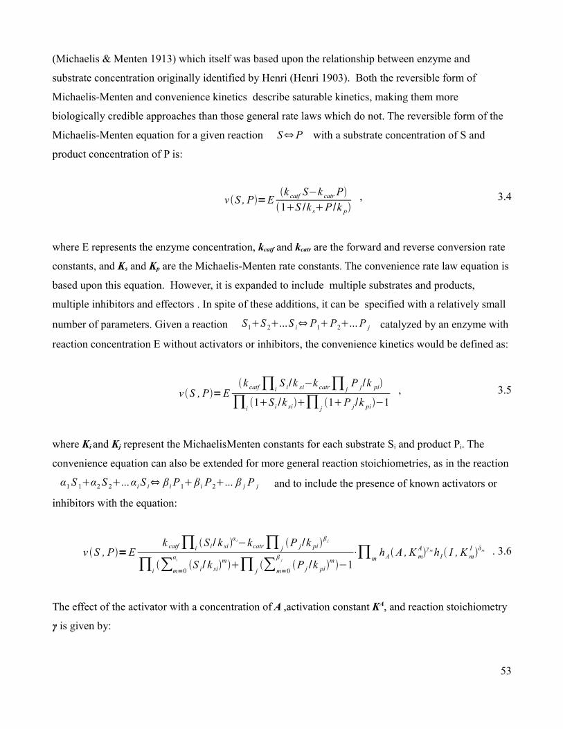
(Michaelis & Menten 1913) which itself was based upon the relationship between enzyme and

substrate concentration originally identified by Henri (Henri 1903). Both the reversible form of

Michaelis-Menten and convenience kinetics describe saturable kinetics, making them more

biologically credible approaches than those general rate laws which do not. The reversible form of the

Michaelis-Menten equation for a given reaction S⇔P with a substrate concentration of S and

product concentration of P is:

v S , P=Ek catf S−k catr P1S /k sP /k p

, 3.4

where E represents the enzyme concentration, kcatf and kcatr are the forward and reverse conversion rate

constants, and Ks and Kp are the Michaelis-Menten rate constants. The convenience rate law equation is

based upon this equation. However, it is expanded to include multiple substrates and products,

multiple inhibitors and effectors . In spite of these additions, it can be specified with a relatively small

number of parameters. Given a reaction S1S 2...S i⇔ P1P2... P j catalyzed by an enzyme with

reaction concentration E without activators or inhibitors, the convenience kinetics would be defined as:

v S , P=Ek catf∏i

S i/k si−k catr∏ jP j/k pi

∏i1S i /k si∏ j

1P j/k pi−1, 3.5

where Ki and Kj represent the MichaelisMenten constants for each substrate Si and product Pi. The

convenience equation can also be extended for more general reaction stoichiometries, as in the reaction

α1 S 1α2 S 2...αi S i⇔ β i P1β i P2... β j P j and to include the presence of known activators or

inhibitors with the equation:

v S , P=Ek catf ∏i S i / k si

α i−kcatr∏ j P j /k pi β j

∏i∑m=0

αi

S i / k sim∏ j

∑m=0

β j

P j /k pim−1

⋅∏mhAA , K m

Aγ m h I I , K mI δm . 3.6

The effect of the activator with a concentration of A ,activation constant KA, and reaction stoichiometry

γ is given by:

53

hA A , K Aγ= AK AA

γ

. 3.7

The effect of an inhibitor with concentration I, inhibition constant KI, and reaction stoichiometry δ is

similarly given by:

h I I , K I δ= IK II

δ

. 3.8

Convenience kinetics' versatility combined with its relatively small number of parameters has made it a

promising source of rate laws for models where the true kinetics are unknown. It and other generalized

rate laws can be automatically added to systems biology models using programs like SBMLsqueezer

(Drager et al. 2008), thus speeding up the generation of simulation ready models. In addition to being

used only for the subset of reactions where the kinetics are unknown, convenience kinetics has also

been successfully used to fully replace all rate laws in models of leucine and valine biosynthesis. This

was done both in an evolutionary algorithms benchmarking study (Drager & M. Kronfeld 2007) and

later was shown to give the best system level results in combination with Michaelis-Menten rate laws

when compared to other methods of assigning approximative rate laws (Draeger et al. 2009) .

Linlog Kinetics

Linlog kinetics is based on concepts from Metabolic Control Analysis (MCA). In MCA, relationships

between various biochemical moieties are described in a mathematical framework. In particular, it

quantifies the dependence of control coefficients on local system properties, called elasticities. Control

coefficients are network dependent properties which relate the effect that a change in a parameter, such

as enzyme activity, has on the relative change in the steady state system variables such as flux.

Elasticities describe the effect that changing the local environment, by altering substrate concentrations

for example, has on the local reaction rate. By quantifying both the local and global effects on control,

MCA demonstrated that control is a distributed property and thus refuted the concept of rate-limiting

steps in biological systems (Kacser & JA Burns 1995; Heinrich & Schuster 1996). Because MCA

quantifies the contributors to flux, it logically seems to be an excellent starting point for a method to

generalize enzyme kinetics. Linlog kinetics is an attempt to do this.

54

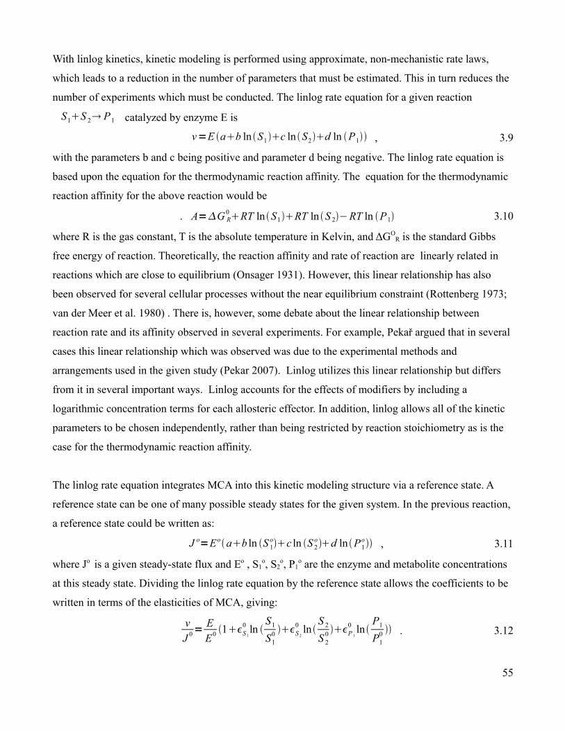
With linlog kinetics, kinetic modeling is performed using approximate, non-mechanistic rate laws,

which leads to a reduction in the number of parameters that must be estimated. This in turn reduces the

number of experiments which must be conducted. The linlog rate equation for a given reaction

S1S 2 P1 catalyzed by enzyme E is

v=E ab ln S1c ln S2d ln P1 , 3.9

with the parameters b and c being positive and parameter d being negative. The linlog rate equation is

based upon the equation for the thermodynamic reaction affinity. The equation for the thermodynamic

reaction affinity for the above reaction would be

. A=G R0RT ln S1RT ln S 2−RT ln P1 3.10

where R is the gas constant, T is the absolute temperature in Kelvin, and ΔGOR is the standard Gibbs

free energy of reaction. Theoretically, the reaction affinity and rate of reaction are linearly related in

reactions which are close to equilibrium (Onsager 1931). However, this linear relationship has also

been observed for several cellular processes without the near equilibrium constraint (Rottenberg 1973;

van der Meer et al. 1980) . There is, however, some debate about the linear relationship between

reaction rate and its affinity observed in several experiments. For example, Pekař argued that in several

cases this linear relationship which was observed was due to the experimental methods and

arrangements used in the given study (Pekar 2007). Linlog utilizes this linear relationship but differs

from it in several important ways. Linlog accounts for the effects of modifiers by including a

logarithmic concentration terms for each allosteric effector. In addition, linlog allows all of the kinetic

parameters to be chosen independently, rather than being restricted by reaction stoichiometry as is the

case for the thermodynamic reaction affinity.

The linlog rate equation integrates MCA into this kinetic modeling structure via a reference state. A

reference state can be one of many possible steady states for the given system. In the previous reaction,

a reference state could be written as:

J o=Eoab ln S 1oc ln S 2

od ln P1o , 3.11

where Jo is a given steady-state flux and Eo , S1o, S2

o, P1o are the enzyme and metabolite concentrations

at this steady state. Dividing the linlog rate equation by the reference state allows the coefficients to be

written in terms of the elasticities of MCA, giving:

vJ 0=

EE0 1S 1

0 ln S1

S10 S 2

0 ln S 2

S 20 P 1

0 ln P1

P10 . 3.12

55

Thus, linlog kinetics can be expressed in terms of elasticities and thereby integrated with MCA by use

of a reference steady state. As an extension of this relationship, it was shown that linlog kinetics could

be successfully employed to determine the control coefficients of a system by applying it to multiple

steady state experiments via linear regression (Wu et al. 2004). Note that for mechanistic enzyme

kinetic rate laws, the elasticities are the partial derivatives of the rate law towards the substrate, product

and effectors.

Linlog kinetics have been successfully used to substitute for the true rate equations in several instances.

Linlog was first demonstrated by Visser et al on an artificial branched network (Visser & J. J. Heijnen

2003a) which was designed by Mendes et al (P. Mendes & Kell 1998). It was subsequently used to

substitute for all of the kinetic equations in the primary metabolism of Esherichia coli (Visser et al.

2004). In addition to these and similar usages, linlog kinetics have been employed as part of a method

to ameliorate constraint-based and kinetic modeling. The resulting method combined flux balance

analysis with linlog kinetics to approximate a yeast model of glycolysis without the need for

experimentally derived kinetic data (Smallbone et al. 2007).

However, in spite of the utility of linlog kinetics in these circumstances, it must be used with caveats.

For one, linlog kinetics are by definition most accurate when near a given reference state (Visser & J. J.

Heijnen 2003a). When concentrations are remote from this state, the linlog approximations may not be

as useful. Indeed, without an appropriate reference state, the linlog equation becomes quite stiff,

making parameter estimation difficult. Finally, it is important to note that the natural logarithm function

will not appropriately mirror the true system kinetics. In biological systems, increasing the substrate

concentrations will increase the reaction rate but not linearly, in fact the rate law saturates and in the

limit of infinite substrate concentration it has a finite rate. This saturation is an effect of the fact that in

a cell (or test tube) there are a finite number of active sites and once all are occupied with substrate, no

other substrate molecules can react, thus leading to the saturation. When saturation occurs, the reaction

rate will asymptotically approach a maximum (Cook & W.W. Cleland 2007). By contrast, the natural

logarithm function applied to a given concentration will tend to infinity as the concentration of

substrate gets very large. All chemical reactions, including those catalyzed by enzymes, have zero rate

when the substrate concentration is zero, however the linlog rate law tends to a negative value when the

substrate concentration approaches zero. Therefore, in order for the linlog rate equations to be

56

applicable, it is important that the relevant concentrations fall within a range where the linlog kinetics

will mirror that of the true kinetics. In particular, kinetics involving extremely large or extremely small

biological concentrations may not be correctly estimated. However, if these constraints are observed,

linlog has been shown to give useful approximations of the true kinetics.

Hypothesis

It is hypothesized here that the convenience kinetics method will provide the overall best

approximation, because it has the form most similar to that of commonly used enzyme rate equations. It

is also thought that generalized mass action kinetics will be the least affected by reducing the available

model information to only include the metabolism reactions. This is hypothesized because mass action

kinetics are believed most affected by local interactions, rather than longer distance ones.

Materials and Methods

Overview

Two models based upon the Claytor network are created for each generalized rate equation method. In

one model, the metabolic portion is separated from the transcriptional and translational portions of the

network in the same manner as in chapter 2. In the second model, these metabolic reactions remain

affiliated with the full Claytor network. In each case, the true rate equations for the metabolic reactions

are replaced with those proposed by the given method. Because there are two forms of the linlog

equation, one where a steady state is directly included and one where it is not, there were more models

needed to test the efficacy of linlog than were needed for the other methods. Therefore, four models

were created to test the linlog generalized rate equation. In one set of linlog models, the form of

equations which included a steady state was applied to the metabolic reactions of both the fully intact

Claytor network and the isolated metabolic portion of this network. In the other set of linlog models,

the form of equations which did not include a steady state was applied to the full and isolated versions

of Claytor network metabolism.

57

These models each have their parameter values estimated via fits to perturbations of M1 concentration,

with a G16 knock out dataset being used for internal validation. All parameter estimation is performed

using the package COPASI (S. Hoops et al. 2006) . The parameter results for each method using the

intact and isolated Claytor metabolism are compared. Finally, the results of each method are compared

using Akaike's Information Criterion (AIC) (Akaike 1974) .

Claytor Network with Altered Kinetics

As was mentioned earlier , it is often not possible to know the true reaction kinetics of a biological

system. Yet, in order to build dynamic models of these systems, knowledge of these rate laws is

essential. Because of the deficiency of kinetic information, several generalized rate laws have been

proposed as a means of circumventing this issue. Of particular interest to this study were convenience

kinetics, linlog kinetics and mass action kinetics. In order to monitor the effect of substituting the true

kinetic rate laws by convenience, linlog, or mass action rate laws , three versions of the full Claytor

network were created. The Clayor artificial biological network was described in detail in chapter 2. In

one version of this altered Claytor network, the true rate laws of the metabolic portion of the Claytor

network are replaced with convenience kinetics where appropriate. In the other versions, these rate

laws are instead substituted with mass action or linlog kinetics. In each case, only the rate laws for the

metabolic portion of the Claytor network were replaced. Tables 3.1 and 3.2 display these metabolic

equations, their true rate law, and the form of the rate law used for each generalized kinetics method.

Of special note is the fact that two forms of the linlog rate equation were used. In one, no knowledge

of a reference state is assumed. In the other, a reference state based on a steady state analysis of the full

Claytor network was used. All steady state and MCA analyzes were performed in COPASI (S. Hoops et

al. 2006).

Table 3.1 : The true rate equations and the generalized kinetics equations which replaced them in each compared method.

Reaction Equation Rate Law Convenience Rate Law LinLog Rate Law Mass Action Rate Law

R1 M1 + M3 = M2 + M4; P13

Bi Bi with Explicit Enzyme

Convenience A+B =P+Q, with Explicit Enzyme

Linlog A+B=P+Q with Explicit Enzyme : with and without reference state

Mass Action A+B = P+Q with Explicit Enzyme

R2 M4 + P15 = P21 + M3; P2



Linlog A+B=P+Q with Explicit Enzyme : with and


58

without reference state

R3 M9 + P21 = P15 + M10; P3





R4 M10 + M11 = M9 + M12; P4





R5 M12 + M20 = M11 + M21; P19





R6 M3 -> M15; P6 Michaelis-Menten with Explicit Enzyme

Convenience A->P with Explicit Enzyme

Linlog A->P with Explicit Enzyme ; with and without reference state

Mass Action A-> P with Explicit Enzyme

R7 M5 + M6 = M3; P12 Bi Uni with Explicit Enzyne

Convenience A+B=P with Explicit Enzyme

Linlog A+B=P with Explicit Enzyme; with and without reference state

Mass Action A+B = P with Explicit Enzyme

R8 M8 + M7 = M6; P9 M3 Bi Uni with Uncooperative Inhibition and Explicit Enzyme

Convenience A+B=P with Explicit Enzyme and Inhibition



R9 M13 + M14 = M7; P10 Bi Uni with Explicit Enzyne

Convenience A+B=P with Explicit Enzyme



R10 M17 + M18 = M13 + M16; P8





R11 M16 + M24 = M17 + M19; P14





R12 M22 = M24; P5 Michaelis-Menten with Explicit Enzyme

Convenience A=P with Explicit Enzyme

Linlog A=P with Explicit Enzyme; with and without reference state

Mass Action A = P with Explicit Enzyme









R19 M1 + M3 = M2 + M4; P16





Table 3.2: The formulas for each rate equation mentioned in Table 3.1.

Rate Law Equation

Bi Bi with Explicit EnzymeE

Kcat f∗A B−P Q /K eq1A /KaP /K p 1B /K bQ /K q

Bi Uni with Explicit EnzyneE

Kcat f∗ A B−P /K eq1A /KaB/ KbP / K p

Bi Uni with Uncooperative Inhibition and Explicit Enzyme E

Kcat f∗ A B−P /K eq1A /K aB/ K bP/ K p∗1 I /K iI

n

Michaelis-Menten with Explicit Enzyme E

Kcat f∗ A−P /Keq1A/K aP/ K p

59

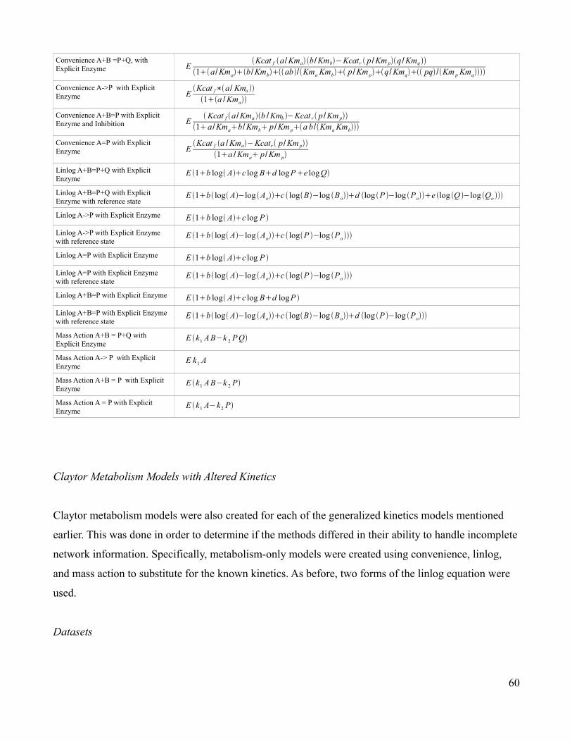
Convenience A+B =P+Q, with Explicit Enzyme E

Kcat f a /Kma b /Kmb−Kcatr p /Km pq /Kmq 1a /Kmab /Kmbab/Kma Kmb p /Km pq /Kmq pq /Km p Kmq

Convenience A->P with Explicit Enzyme E

Kcat f∗a/ Kma 1a /Kma

Convenience A+B=P with Explicit Enzyme and Inhibition E

Kcat f a /Kma b /Kmb −Kcat r p /Km p1a /Kmab/Kmb p /Km pa b /Kma Kmb

Convenience A=P with Explicit Enzyme E

Kcat f a /Kma−Kcatr p/Km p1a /Kma p/Km p

Linlog A+B=P+Q with Explicit Enzyme

E 1b log Ac log Bd log Pe log Q

Linlog A+B=P+Q with Explicit Enzyme with reference state

E 1b log A−log Aoc logB−log Bod log P −log Poe log Q −log Qo

Linlog A->P with Explicit Enzyme E 1b log Ac log P

Linlog A->P with Explicit Enzyme with reference state

E 1b log A−log Aoc logP −log Po

Linlog A=P with Explicit Enzyme E 1b log Ac log P

Linlog A=P with Explicit Enzyme with reference state

E 1b log A−log Aoc logP −log Po

Linlog A+B=P with Explicit Enzyme E 1b log Ac log Bd logP

Linlog A+B=P with Explicit Enzyme with reference state

E 1b log A−log Aoc logB−log Bod log P −log Po


E k1 A B−k 2 P Q

Mass Action A-> P with Explicit Enzyme

E k1 A


E k1 A B−k 2 P


E k1 A−k2 P

Claytor Metabolism Models with Altered Kinetics

Claytor metabolism models were also created for each of the generalized kinetics models mentioned

earlier. This was done in order to determine if the methods differed in their ability to handle incomplete

network information. Specifically, metabolism-only models were created using convenience, linlog,

and mass action to substitute for the known kinetics. As before, two forms of the linlog equation were

used.

Datasets

60

Two datasets were used in order to estimate the parameters for all models in the current study. One

dataset , a metabolic perturbation, is used as a training set, while the other, a genetic perturbation, is

used as an internal validation set. The training set consists of a series of perturbations of the

concentration of metabolite M1. The validation dataset is formed from a time-series produced after

knocking out gene G16. Both of these datasets are described in greater detail in chapter 2.


The parameter values for each of the generalized kinetics models were obtained via minimizing the

sum of squares of the residuals between the simulated data and the measured data. The numerical

minimization methods used were the particle swarm (Clerc & Kennedy 2002; Kennedy & Eberhart

1995) and genetic algorithm with stochastic ranking (GASR) (Goldberg 1989). These stochastic

methods were preferred as they have less of a tendency of becoming trapped in local minima. In order

to prevent the possibility of overflow in the optimization of the mass action functions, parameter

estimation was performed iteratively. The analysis was at first restricted to a narrow range near the

starting point. If a boundary was approached during successive runs, the range for that parameter was

increased. Parameter estimation was performed until there was no or minimal improvement in the

overall sum of squares results for the model.

For the convenience kinetics models, the starting values and initial search range were based upon the

true kinetics values when applicable. These values were approximated using the parameter values of

the true rate equations. The linlog parameter range was based upon elasticities taken from a MCA

analysis of the full Claytor network. When the form of the linlog equation which did not require a

reference state was employed, this range was increased to account for this lack. The mass action

kinetics models, by contrast, used a range of 0 to 2000 for all parameters. This parameter range is based

upon the ranges observed in parameter values that were obtained experimentally and are stored in the

the BRENDA enzyme database (Chang et al. 2009; I. Schomburg et al. 2002), and was also used as the

range for the generalized kinetics comparisons made by Drager et al (Draeger et al. 2009) .

Comparison of Parameter Values Estimated in Intact and in Isolated Claytor Network Metabolism

61

In order to compare the parameter value estimates obtained using the intact and isolated Claytor

metabolic network, the paired Wilcoxon signed rank test was used. The Wilcoxon signed rank test, with

test statistic W, is a nonparametric test for the null hypothesis, H0 , that the difference between two

values is equal to 0 (Whitley & Ball 2002) . The values for W as well as their associated p-values were

obtained using the R statistics package (R Development Core Team 2009). The Wilcoxon signed rank

test was used to compare the overall parameter value differences between the intact and isolated

Claytor metabolism models for each method. In addition, the parameter values for individual reactions

were also compared.

Determining Individual Model Performance

The quality of fit obtained by each generalized kinetics method was determined in the same way as

discussed in chapter 2. In brief, the fits of each dependent variable of metabolism are assessed using

both the individual sum of squares value for that variable as well as a quality bit score. The quality bit

score is a binary bit string which assesses the qualitative fit of the model to the data. It assigns a 1 or 0

to the following fit properties: overall fit, shape, scale, direction, and alignment. Although the quality

bit score is somewhat subjective, it is useful for ascertaining how well the given model reflects the

data.

Comparison of Models Employing Differing Generalized Rate Laws

The final models obtained via each of the generalized kinetics methods were compared using Akaike's

Information Criterion (AIC). The AIC compares model performance based upon both the sum of

squares values and the number of model parameters, where preference is given to more parsimonious

models. The form of the AIC equation used in this study was:

AIC=N ln SSQ /N 2k , 3.13

where k represents the number of parameters, N is the number of observed data points, and SSQ is the

residual sum of squares. Comparisons of each generalized kinetics method were made by applying AIC

to all isolated and all intact Claytor metabolism models.

62


Linlog Kinetics Model

As mentioned in the materials and methods section, two different forms of the linlog rate equation were

used. One required information from a reference state and the other did not. Both models were used in

the attempt to estimate their parameter values. However, neither parameter estimation converged. This

result was seen both in the models where the non-metabolic reactions remained intact as well as in the

models where metabolism was studied in isolation.

Two hypotheses emerged as to why linlog was unable to correctly fit the Claytor network data. One

possibility was that the range over which parameter estimation was performed was too large (and

therefore convergence could happen if the methods were allowed to run for much longer time). The

other possibility was that the Claytor lake model itself contained features which made it impossible to

being fit by linlog kinetics. Both hypotheses were tested by inserting individual reactions containing

linlog rate equations into the full Claytor network and then attempting to estimate their parameters.

This means that at each time only one linlog rate law was being estimated since all other reactions were

the original ones (i.e. the true kinetics). By inserting one reaction at a time into a network where all

other kinetics were known, the search space should be reduced. Rather than fitting parameters from all

of metabolism, only one reaction was parametrized in this exercise. Once this reaction was

parametrized sufficiently, the values obtained could be used as the basis for the parameter range in a

new fit. Insertion and parameter estimation of individual reactions into a fully described model also had

the benefit of testing whether all reactions could be fit using linlog kinetics. The results of this can be

seen in table 3.3. While not all reactions could be fit using this methodology, most were. In some cases,

reactions could not be fit using the more general form of the linlog equation, but were able to be fit

when a reference state was used. Therefore, it may be concluded that these reactions, specifically R8

and R10, require more information in order to be defined using linlog kinetics. By contrast, reactions

R1 and R19 were not fit by substituting either form of the linlog equation into the full Claytor network.

It is likely that certain aspects of these reactions make them impossible to model using linlog kinetics.

In both cases, all of the component's elasticities within the context of the reaction at the reference state

63

were zero. Because linlog parameters are equivalent to the elasticities when a reference state is

incorporated, when all of the relevant elasticities are zero linlog fits the reaction kinetics as a constant.

In both reactions R1 and R19, this is inappropriate. Reactions R1 and R19 constitute an important

feature of the Claytor network. They make up the reaction cycle which detoxifies M1. Although linlog

kinetics has had much success in estimating rate equations in a variety of organisms, these were often

branched systems and did not include loop structures. It has been shown that feedback loops require

multiple steady state perturbations for their elasticities to be identifiable (Kacser & J. A. Burns 1979;

Giersch 1994; Giersch & CornishBowden 1996). Therefore, it is likely that in order for linlog kinetics

to correctly approximate feedback loops, a combination of reference states would be needed for each

participating reaction. As feedback loops comprise an important part of biological systems (Alberts et

al. 2007; Iyengar & Bhalla 1999; Reeves & Fraser 2009), it is unlikely that linlog kinetics will remain

relevant without addressing this issue.

These results confirm that, in large part, the lack of convergence in the estimation of all linlog

parameters simultaneously was due to the size of the search space, since it was possible to estimate

parameters of most linlog reactions when done in isolation. However, for two reactions, the problem

was also the unidentifiability of the parameters (i.e. due to characteristics of the data and the equation).

Table 3.3 : Effectiveness of modeling individual metabolic reactions with linlog kinetics

Reaction Equation Fit Using Linlog Fit Using Linlog Containing Reference State

R1 M1 + M3 = M2 + M4; P13 no no

R2 M4 + P15 = P21 + M3; P2 yes yes

R3 M9 + P21 = P15 + M10; P3 yes yes

R4 M10 + M11 = M9 + M12; P4 yes yes

R5 M12 + M20 = M11 + M21; P19

yes yes

R6 M3 -> M15; P6 yes yes

R7 M5 + M6 = M3; P12 yes yes

R8 M8 + M7 = M6; P9 M3 no yes

R9 M13 + M14 = M7; P10 yes yes

R10 M17 + M18 = M13 + M16; P8 no yes

R11 M16 + M24 = M17 + M19; P14

yes yes

R12 M22 = M24; P5 yes yes

64

R13 M23 = M22; P20 yes yes

R14 M22 = M20; P7 yes yes

R19 M1 + M3 = M2 + M4; P16 no no

Convenience Kinetics Applied to Intact Claytor Network Metabolism

Convenience kinetics were used as approximations for the rate equations of the metabolic portion of

the Claytor network. The remainder of the network was left intact. The results of parameter estimation

with these approximative rate laws can be seen in tables 3.4 and 3.5 below. As before, the experiment

with the lowest sum of squares and the one with the highest were chosen for further analysis. The

quality bit score for the dependent variables of each of these experiments is given along with the sum

of squares values. A low sum of squares value, in this case, does not always have a corresponding high

quality bit score as can be seen by M20.

Table 3.4 : Residual sum of squares of fits to experiments using convenience kinetics as applied to full Claytor network.


1 0.05 5.58E-03

2 0.10 6.15E-03

3 0.15 7.02E-03

4 0.20 7.69E-03

5 0.25 7.32E-03

Table 3.5 : Residual sum of squares of fits to each dependent variable of metabolism and the corresponding quality bit score

obtained in experiments 1 and 4.

Dependent Value

Sum of Squares


M1 3.90E-03 00110 00110

M3 8.65E-04 00010 00010

M2 1.77E-02 01010 01010

M4 1.38E-04 00000 00000

M9 5.81E-05 00110 00110

M10 3.52E-04 00110 00110

M11 1.24E-04 00110 00110

65

M12 3.86E-04 00110 00110

M20 9.30E-06 00000 00000

M6 2.17E-03 00010 00010

M7 6.57E-03 00010 00010

M13 1.07E-03 11110 11110

M17 4.19E-05 00100 00100

M16 3.79E-04 00100 00100

M22 4.15E-07 00010 00010

M24 2.45E-05 00010 00010

P15 4.44E-06 01010 01010

P21 1.25E-05 01110 01110

The dependent variables which achieved the lowest quality bit scores were M20 and M4. Neither of

these received the highest sum of squares estimate, which was achieved by M2. Overall, the sum of

squares values for the dependent variables are good. However, the qualitative aspects of each fit as

assessed by quality bit score are not particularly good.

Convenience Kinetics Applied to Isolated Claytor Network Metabolism

The quality of fit was also examined for convenience kinetics applied to the isolated metabolic portion

of the Claytor network. The results of this fit can be seen below in tables 3.6 and 3.7.

Table 3.6 : Residual sum of squares for each fit to experiments using convenience kinetics applied to the isolated metabolic

portion of the Claytor network


1 0.05. 1.41E-03

2 0.10 2.94E-03

3 0.15 4.36E-03

4 0.20 5.58E-03

5 0.25 5.93E-03

Table 3.7 : Residual sum of squares for fits to each dependent variable of metabolism and the corresponding quality bit scores

obtained in experiments 1 and 5

66

Dependent Value

Sum of Squares


M1 9.01E-05 11111 11111

M3 8.69E-04 00000 00000

M2 3.65E-05 11111 11111

M4 1.38E-04 00000 00000

M9 5.81E-05 00110 00110

M10 3.52E-04 00110 00110

M11 1.24E-04 00110 00110

M12 3.86E-04 00110 00110

M20 9.93E-06 00000 00000

M6 2.18E-03 00000 00000

M7 6.63E-03 00010 00010

M13 8.85E-03 10110 10110

M17 4.20E-05 00100 00100

M16 3.80E-04 00100 00100

M22 1.09E-05 00000 00000

M24 1.71E-05 00000 00000

P15 3.86E-05 01110 01110

P21 1.25E-05 01110 01110

The overall fit quality of the convenience kinetics method applied to the metabolic portion of the

Claytor network is similar to that obtained using the fully intact model. In the case of several

metabolites, for example M1 and M2, the fit achieved is actually better than that obtained using the full

network.

Comparison of Convenience Kinetics Parameters in Intact and in Isolated Metabolism of Claytor

Network

In table 3.8, a comparison is given between the convenience kinetics parameters which were estimated

using the full Claytor network and those which were determined using the metabolic portion in

isolation. The signed pairwise Wilcoxon W for the overall comparison was W=1415, with a p-value of

P = 0.5356 using the two-tailed distribution. Therefore, the parameter values obtained using the intact

and isolated Claytor network metabolism do not differ at the α = 0.05 level of significance. None of the

comparisons performed on individual reactions was significant at this level either. Reaction R4 was

67

closest to having significantly different parameter values with a Wilcoxon p-value of P = 0.063

Table 3.8 : Comparison between the convenience kinetics parameter values obtained using the intact and isolated Claytor

metabolism network

Reaction Equation Parameter Intact Claytor Metabolism

Estimate

Isolated Claytor Metabolism

Estimate

Wilcoxon W Wilcoxon p-value

R1 M1 + M3 = M2 + M4; P13 Kcatf 23841 25465 12 0.844

Kcatr 2758 2025.75

Kma 0.084582 0.014721

Kmb 0.052174 0.10131

Kmx 2.86788 2.85725

Kmy 0.015881 0.005314

R2 M4 + P15 = P21 + M3; P2 Kcatf 409.024 1310.66 5 0.313

Kcatr 734.076 1411.89

Kma 0.019326 0.030204

Kmb 0.002745 0.002458

Kmx 0.004228 0.00493

Kmy 0.44848 0.230401

R3 M9 + P21 = P15 + M10; P3 Kcatf 13236.4 19112.8 11 1

Kcatr 1792.26 1462.23

Kma 0.021653 0.031312

Kmb 0.001159 0.000926

Kmx 0.010878 0.004181

Kmy 0.000543 0.000421

R4 M10 + M11 = M9 + M12; P4 Kcatf 2273.32 3225.44 1 0.063

Kcatr 2641.2 2864.77

Kma 0.002334 0.002127

Kmb 0.011703 0.013106

Kmx 0.01704 0.046201

Kmy 0.016144 0.017126

R5 M12 + M20 = M11 + M21; P19 Kcatf 121.164 101.392 18 0.156

Kcatr 554.954 384.499

Kma 0.000138 0.000133

Kmb 0.280794 0.392881

Kmx 0.009671 0.007587

Kmy 8.84385 1.21907

R6 M3 -> M15; P6 Kcatf 127.07 63.4065 2 1

Kma 0.002179 0.003746

R7 M5 + M6 = M3; P12 Kcatf 89.8539 239.268 5 0.625

Kcatr 3057.78 2103.25

68

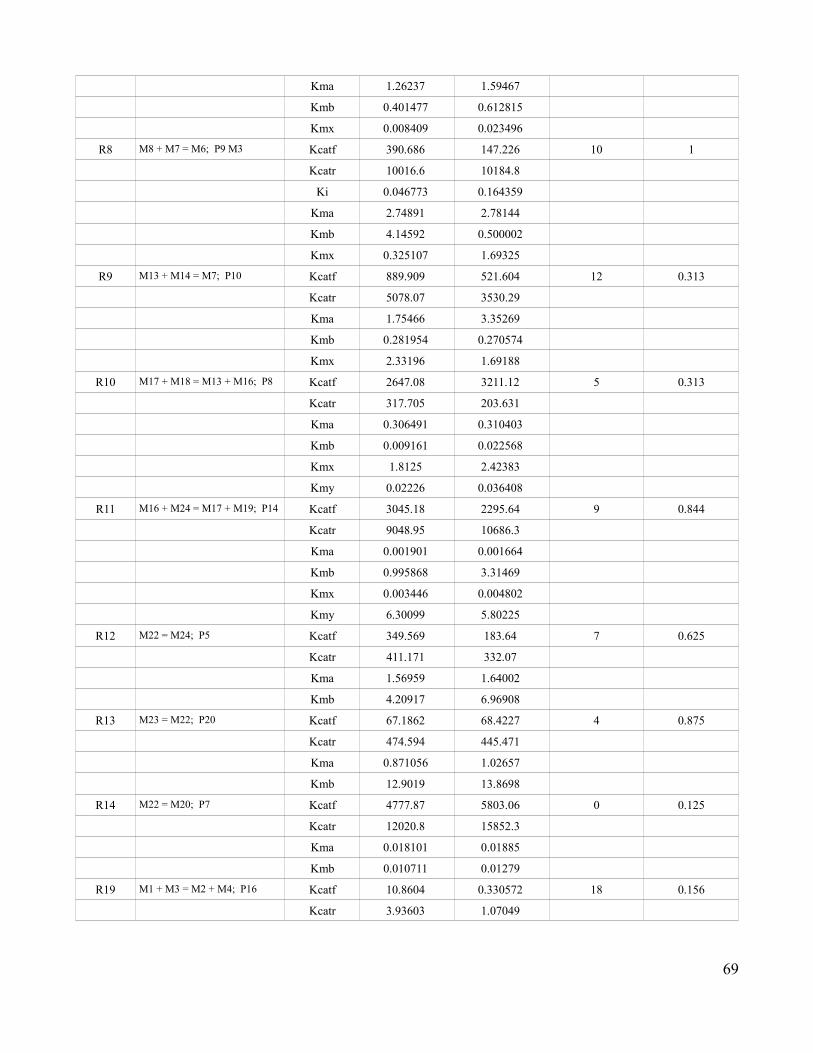
Kma 1.26237 1.59467

Kmb 0.401477 0.612815

Kmx 0.008409 0.023496

R8 M8 + M7 = M6; P9 M3 Kcatf 390.686 147.226 10 1

Kcatr 10016.6 10184.8

Ki 0.046773 0.164359

Kma 2.74891 2.78144

Kmb 4.14592 0.500002

Kmx 0.325107 1.69325

R9 M13 + M14 = M7; P10 Kcatf 889.909 521.604 12 0.313

Kcatr 5078.07 3530.29

Kma 1.75466 3.35269

Kmb 0.281954 0.270574

Kmx 2.33196 1.69188

R10 M17 + M18 = M13 + M16; P8 Kcatf 2647.08 3211.12 5 0.313

Kcatr 317.705 203.631

Kma 0.306491 0.310403

Kmb 0.009161 0.022568

Kmx 1.8125 2.42383

Kmy 0.02226 0.036408

R11 M16 + M24 = M17 + M19; P14 Kcatf 3045.18 2295.64 9 0.844

Kcatr 9048.95 10686.3

Kma 0.001901 0.001664

Kmb 0.995868 3.31469

Kmx 0.003446 0.004802

Kmy 6.30099 5.80225

R12 M22 = M24; P5 Kcatf 349.569 183.64 7 0.625

Kcatr 411.171 332.07

Kma 1.56959 1.64002

Kmb 4.20917 6.96908

R13 M23 = M22; P20 Kcatf 67.1862 68.4227 4 0.875

Kcatr 474.594 445.471

Kma 0.871056 1.02657

Kmb 12.9019 13.8698

R14 M22 = M20; P7 Kcatf 4777.87 5803.06 0 0.125

Kcatr 12020.8 15852.3

Kma 0.018101 0.01885

Kmb 0.010711 0.01279

R19 M1 + M3 = M2 + M4; P16 Kcatf 10.8604 0.330572 18 0.156

Kcatr 3.93603 1.07049

69

Kma 0.858299 0.935993

Kmb 0.097779 0.043981

Kmx 2.87793 2.68964

Kmy 0.004153 0.001

Mass Action Kinetics Applied to Intact Claytor Network Metabolism

Mass action is a classic method for representing chemical kinetics. Because it does not take enzyme

actions into account, it generally requires the determination of elementary reactions to be effective. In

this study, a general form of mass action kinetics was used to model the rates of each metabolic

reaction. Each reaction rate was multiplied by the relevant enzyme concentration (which is know from

the original Claytor network, and in a real experiment would have to be determined). However, all

reactions remained in their original form and no elementary reactions were considered. The quality of

fitting results obtained using generalized mass action kinetics on the intact Claytor network are given in

tables 3.9 and 3.10. Experiments 2 and 5 are used in comparisons as they show the widest

discrepancies in the sum of squares values, although not in initial M1 concentration.

Table 3.9 : Residual sum of squares for each fit by experiment where generalized mass action kinetics is applied to full Claytor

network


1 0.05 1.69E-03

2 0.10 7.63E-04

3 0.15 8.57E-04

4 0.20 1.19E-03

5 0.25 1.73E-03

Table 3.10 : Residual sum of squares for each dependent variable of metabolism and the quality bit score for experiments 2 and 5

Dependent Value Sum of Squares Experiment 2 Fit Quality Bit String

Experiment 5 Fit Quality Bit String

M1 3.50E-05 11111 11111

M3 1.35E-04 11110 11110

M2 1.07E-05 11111 11111

M4 1.56E-04 00100 00100

70

M9 1.31E-05 00110 00110

M10 8.95E-05 00110 00110

M11 2.02E-05 00110 00110

M12 6.92E-05 00110 00110

M20 1.31E-05 00000 00000

M6 1.94E-04 11110 11110

M7 5.68E-04 11110 11110

M13 4.61E-03 11110 11110

M17 3.59E-06 00110 00110

M16 3.27E-05 00110 00110

M22 2.70E-04 00000 00000

M24 1.20E-07 00100 00100

P15 1.84E-08 11111 11111

P21 1.25E-05 01010 01010

As can be seen in table 3.10, both the sum of squares values and the quality bit scores for most of the

fitted dependent variables is fairly good. This is somewhat surprising as generalized mass action was

one of the simpler methods used.

Mass Action Kinetics Applied to Isolated Claytor Network Metabolism

The fit quality results for applying generalized mass action to the isolated metabolic portion of the

Claytor network are shown below in tables 3.11 and 3.12.

Table 3.11: Residual sum of squares values for the fits to each experiment using mass action kinetics applied to isolated Claytor

metabolism model


1 0.05 4.00E-04

2 0.10 9.01E-04

3 0.15 1.23E-03

4 0.20 1.71E-03

5 0.25 2.57E-03

Table 3.12 : Residual sum of squares for fits to each dependent variable of metabolism where mass action applied to the isolated

Claytor metabolism model and the associated fit quality bit score achieved in experiments 1 and 5

71

Dependent Value Sum of Squares Experiment 1 Fit Quality Bit String

Experiment 5 Fit Quality Bit String

M1 1.28E-04 11110 11110

M3 7.97E-05 10110 10110

M2 3.88E-05 11111 11110

M4 1.26E-04 00110 00110

M9 1.27E-05 00110 00110

M10 8.65E-05 00110 00110

M11 5.58E-05 00110 00110

M12 1.95E-04 00110 00110

M20 1.33E-06 00000 00000

M6 1.90E-04 10110 10110

M7 6.00E-04 10110 10110

M13 4.79E-03 10110 10110

M17 4.88E-05 00110 00110

M16 4.40E-04 00110 00110

M22 8.04E-07 00000 00000

M24 2.60E-06 00000 00000

P15 7.98E-07 00110 00110

P21 1.20E-05 01010 01010

The results obtained are very similar to those obtained by applying generalized mass action kinetics to

the full Claytor network. However, in several cases the fits obtained using the intact Claytor network

are better than those obtained here.

Comparison of Mass Action Kinetics Parameters in Intact and in Isolated Metabolism of Claytor

Network

The parameter values obtained using the intact and isolated Claytor network metabolism were

compared using the Wilcoxon signed rank test. The pairwise Wilcoxon W for the overall comparison

between the isolated and intact Claytor metabolism parameters is W= 193, with a p-value of P =

0.6089 using the two-tailed distribution. Therefore, there is no difference between the two sets of

parameters at the α = 0.05 level of significance. The differences in the parameter values obtained using

the intact and isolated metabolic portions of the Claytor network were also assessed for each reaction.

These results are shown below in table 3.13. In no case were any of the Wilcoxon p-values for these

differences close to the predetermined significance level.

72

Table 3.13 : Comparison between the generalized mass action kinetics parameter values obtained using the intact and isolated Claytor

metabolism network

Reaction Equation Parameter Intact Claytor Metabolism

Estimate

Isolated Claytor Metabolism

Estimate

Wilcoxon W Wilcoxon p-value

R1 M1 + M3 = M2 + M4; P13 K1 511.625 17.1905 1 1

K2 50.8187 1356.79

R2 M4 + P15 = P21 + M3; P2 K1 766.447 1999.99 0 0.5

K2 615.397 843.489

R3 M9 + P21 = P15 + M10; P3 K1 1601.3 1331.13 1 1

K2 410.809 780.591

R4 M10 + M11 = M9 + M12; P4

K1 1876.45 1414.79 3 0.5

K2 1454.43 437.275

R5 M12 + M20 = M11 + M21; P19

K1 1659.93 1342.75 1 1

K2 847.193 1709.66

R6 M3 -> M15; P6 K1 976.05 0.008269 1 1

R7 M5 + M6 = M3; P12 K1 959.421 1704.14 0 0.5

K2 1408.18 1949.3

R8 M8 + M7 = M6; P9 M3 K1 1121 165.16 3 0.5

K2 1907.98 275.087

R9 M13 + M14 = M7; P10 K1 1173.45 1337.79 0 0.5

K2 942.408 1066.14

R10 M17 + M18 = M13 + M16; P8

K1 792.183 452.936 2 1

K2 317.589 1996.87

R11 M16 + M24 = M17 + M19; P14

K1 1703.04 1985.09 0 0.5

K2 620.324 159.536

R12 M22 = M24; P5 K1 1869.82 1794.08 3 0.5

K2 772.203 779.669

R13 M23 = M22; P20 K1 1391.84 1864.14 0 0.5

K2 697.072 885.376

R14 M22 = M20; P7 K1 369.717 339.94 1 1

K2 1497.65 1430.42

R19 M1 + M3 = M2 + M4; P16 K1 967.457 1884.15 1 1

K2 1720.9 1943.64

Comparison Between Generalized Kinetics Methods Applied to Metabolism in Intact Claytor Network

73

In table 3.14, the convenience and generalized mass action kinetics methods applied to the fully intact

Claytor network metabolism are compared using their AIC values. The generalized mass action model

is preferred in this instance as it achieves the lowest AIC value.

Table 3.14 : A comparison of the fits of convenience and generalized mass action models applied to the intact Claytor metabolic

network

Generalized Kinetics Method

Sum of Squares Number of Parameters AIC

Convenience 3.38E-02 219 2.05E+06

Mass Action 6.23E-03 170 1.57E+06

Comparison Between Varying Kinetics Methods Applied to Isolated Metabolism Model of Claytor

Network

The results of the comparison between the convenience and mass action kinetics models fitted to the

isolated metabolic portion of the Claytor network is shown below in table 3.15. In addition, the results

obtained using the true kinetic rate equations are shown for comparison. In this case, the generalized

mass action model would be again selected, even over that of the model which used the true form of the

rate equations. This preference is due to the smaller number of parameters employed by the mass action

model as well as its low sum of squares value.

Table 3.15 : Results of comparing models formed using the true rate equations, convenience, and generalized mass action kinetics

applied to isolated metabolic portion from the Claytor network

Kinetics Method Sum of Squares Number of Parameters AIC

True 6.44E-03 79 6.94E+05

Convenience 2.02E-02 78 6.90E+05

Mass Action 6.81E-03 29 2.14E+05

74

Conclusions

The goal of this study was to compare three different methods for modeling unknown kinetic rate laws:

convenience, linlog, and generalized mass action. As the modeling demand for rate equations increases

while the number determined in vivo does not, there is an increasing need to evaluate the performance

of generalized rate equations. An advantage of the current study is its use of the Claytor artificial

biological network. The Claytor network contains many of the complex features found in natural

biological networks and is thus a useful tool for testing these methods. These complex interactions

made it possible to identify weaknesses in certain methods. In particular, it was shown than the

parameter values for the linlog approximation could not converge when applied to the Claytor network

data. This is likely due to its inability to handle feedback loops, which are a common feature in many

biological systems. Thus, this study illustrates that care must be taken when employing linlog to certain

datasets. In addition, it seems to indicate that there is a need to prove generalized kinetics methods

upon artificial biological networks which contain higher degrees of complexity.

It was hypothesized that the convenience kinetics method would perform best overall due to its

closeness in equation structure to that of the true rate equations. This hypothesis was not supported by

the results of the current study. Surprisingly, generalized mass action kinetics performed the best when

applied to the fully intact as well as when applied to isolated portions of the Claytor metabolic network.

When applied to the isolated Claytor network metabolism, it also outperformed the parameter results

estimated using the true rate equations. Interestingly, the true model and the convenience model

performed similarly on the isolated Claytor network metabolism. Therefore, convenience kinetics is

still a useful method for generalizing rate equations in this situation, as it gives results similar to those

of the true model.

It was also hypothesized that the generalized mass action model would be the least affected by being

restricted to the isolated metabolic portion of the Claytor network. Neither the generalized mass action

nor the convenience kinetics model parameters was significantly affected by being thus restricted.

However, the Wilcoxon p-value for the generalized mass action model was slightly larger, indicating

that it was sightly less affected. Therefore, this hypothesis is supported.

75

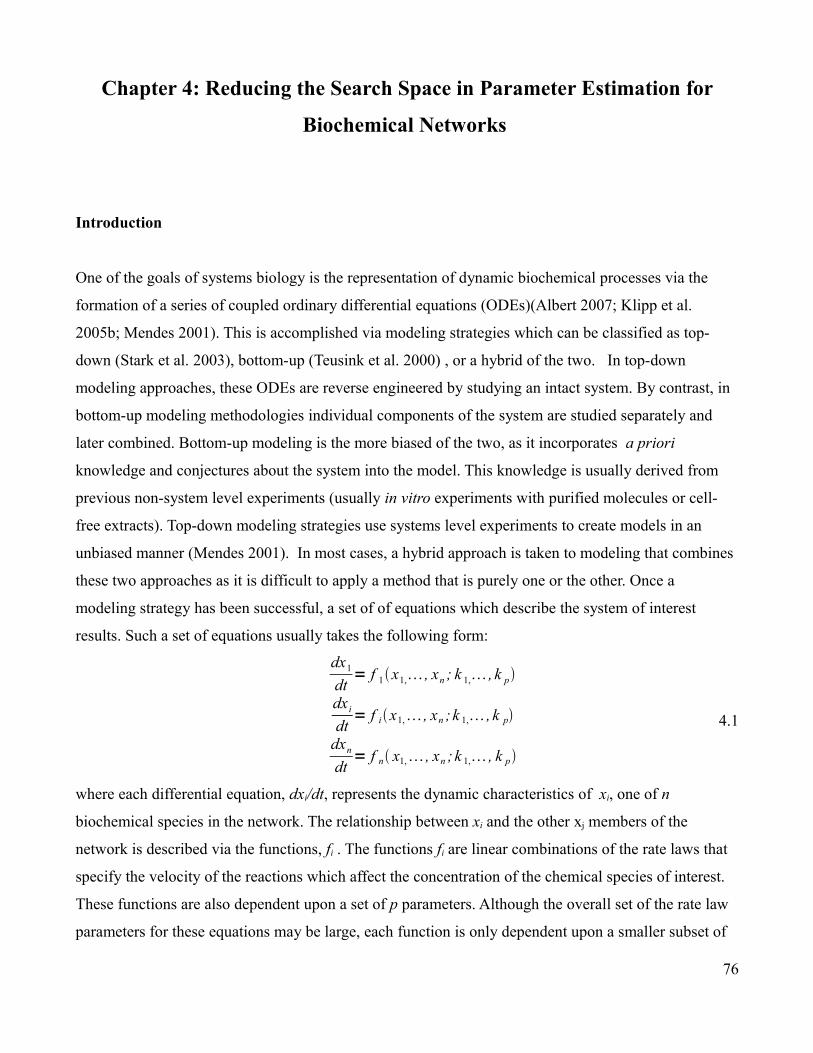
Chapter 4: Reducing the Search Space in Parameter Estimation for

Biochemical Networks

Introduction

One of the goals of systems biology is the representation of dynamic biochemical processes via the

formation of a series of coupled ordinary differential equations (ODEs)(Albert 2007; Klipp et al.

2005b; Mendes 2001). This is accomplished via modeling strategies which can be classified as top-

down (Stark et al. 2003), bottom-up (Teusink et al. 2000) , or a hybrid of the two. In top-down

modeling approaches, these ODEs are reverse engineered by studying an intact system. By contrast, in

bottom-up modeling methodologies individual components of the system are studied separately and

later combined. Bottom-up modeling is the more biased of the two, as it incorporates a priori

knowledge and conjectures about the system into the model. This knowledge is usually derived from

previous non-system level experiments (usually in vitro experiments with purified molecules or cell-

free extracts). Top-down modeling strategies use systems level experiments to create models in an

unbiased manner (Mendes 2001). In most cases, a hybrid approach is taken to modeling that combines

these two approaches as it is difficult to apply a method that is purely one or the other. Once a

modeling strategy has been successful, a set of of equations which describe the system of interest

results. Such a set of equations usually takes the following form:

dx1

dt= f 1x1, , xn ; k 1, , k p

dx i

dt= f ix1, , xn ;k 1, , k p

dxn

dt= f n x1, , xn ;k 1, , k p

4.1

where each differential equation, dxi/dt, represents the dynamic characteristics of xi, one of n

biochemical species in the network. The relationship between xi and the other xj members of the

network is described via the functions, fi . The functions fi are linear combinations of the rate laws that

specify the velocity of the reactions which affect the concentration of the chemical species of interest.

These functions are also dependent upon a set of p parameters. Although the overall set of the rate law

parameters for these equations may be large, each function is only dependent upon a smaller subset of

76

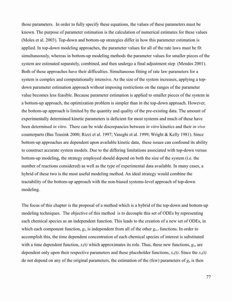
those parameters. In order to fully specify these equations, the values of these parameters must be

known. The purpose of parameter estimation is the calculation of numerical estimates for these values

(Moles et al. 2003). Top-down and bottom-up strategies differ in how this parameter estimation is

applied. In top-down modeling approaches, the parameter values for all of the rate laws must be fit

simultaneously, whereas in bottom-up modeling methods the parameter values for smaller pieces of the

system are estimated separately, combined, and then undergo a final adjustment step (Mendes 2001).

Both of these approaches have their difficulties. Simultaneous fitting of rate law parameters for a

system is complex and computationally intensive. As the size of the system increases, applying a top-

down parameter estimation approach without imposing restrictions on the ranges of the parameter

value becomes less feasible. Because parameter estimation is applied to smaller pieces of the system in

a bottom-up approach, the optimization problem is simpler than in the top-down approach. However,

the bottom-up approach is limited by the quantity and quality of the pre-existing data. The amount of

experimentally determined kinetic parameters is deficient for most systems and much of these have

been determined in vitro. There can be wide discrepancies between in vitro kinetics and their in vivo

counterparts (Bas Teusink 2000; Rizzi et al. 1997; Vaseghi et al. 1999; Wright & Kelly 1981). Since

bottom-up approaches are dependent upon available kinetic data, these issues can confound its ability

to construct accurate system models. Due to the differing limitations associated with top-down versus

bottom-up modeling, the strategy employed should depend on both the size of the system (i.e. the

number of reactions considered) as well as the type of experimental data available. In many cases, a

hybrid of these two is the most useful modeling method. An ideal strategy would combine the

tractability of the bottom-up approach with the non-biased systems-level approach of top-down

modeling.

The focus of this chapter is the proposal of a method which is a hybrid of the top-down and bottom-up

modeling techniques. The objective of this method is to decouple this set of ODEs by representing

each chemical species as an independent function. This leads to the creation of a new set of ODEs, in

which each component function, gi, is independent from all of the other gn-1 functions. In order to

accomplish this, the time dependent concentration of each chemical species of interest is substituted

with a time dependent function, xi(t) which approximates its role. Thus, these new functions, gn, are

dependent only upon their respective parameters and these placeholder functions, xn(t). Since the xn(t)

do not depend on any of the original parameters, the estimation of the (few) parameters of gn is then

77

independent of the other parameters. The parameters for the functions gn can therefore be estimated

independently and used to restrict the parameter search space within the original coupled set of ODEs.

It is hypothesized that employing this method will result in two main benefits. First, it will allow the

parameters of the functions fn to be estimated in less time. It is thought that a reduced amount of time

will be necessary to estimate the parameter values because the parameter space to search by the

optimizing methods is much smaller dimension. Thus, it is believed that the more this space can be

restricted the less time the parameter estimation will take. Secondly, it is hypothesized that in certain

systems these values may be more accurate than those estimates performed without the benefit of a

restricted search range. Depending upon the biochemical system of interest , the amount of data

necessary to fully and accurately specify a model of it , as represented by ODEs, can be quite large. In

cases where there is not enough data, the model becomes underdetermined (Albert 2007). In this

situation, many parameter estimates will fit the available data, even if they are not near the correct

values. By reducing the search space, it is thought that this problem will be minimized somewhat as

there will be less search space for the parameter estimation methods to fall into one of these local

minima.

Method

Overview

The goal of the proposed method is to decrease the time necessary to estimate the parameter values of a

biochemical network by reducing the parameter search space. It is proposed that this may be achieved

by transforming the representative set ODEs into an independent set of ODEs. This will allow the

parameters on the right hand side of the new ODEs to be fit separately. After obtaining the estimates for

the parameters of the new ODEs, this information can be used to inform the parameter estimation of the

original system of ODEs.

This ODE decoupling is achieved via a process of substituting time dependent functions for each of the

concentrations of the member biochemical species in each of the original fn functions. These new

functions do not need to represent structural properties of the underlying biochemical system, as do the

78

original. Rather, they only need to be time dependent and fit the available dynamic data. Thus, in the

new functions, gn, these concentrations are represented as being dependent upon time, but not of each

other. In the auxiliary representation of the biochemical system, these new gn functions on the right

hand side contain different parameters from the original p parameters of their counterparts in fn.

Importantly, these parameters will have different values in each of the gn functions, which will allow

them to be assessed individually. These new representations take the general form:

x1 t =g1 t ;a1,1 , ,a1, lx i t =g it ;a i ,1 ,,a i , l

xn t =gn t ;an,1 , ,an ,l

4.2

These functions g and their parameters a should be able to accurately reproduce the time series of the

corresponding xi(t). Once these functions and their constituent parameters have been identified, then

this information can be used to estimate the k parameter values used in fi independent from the

remaining k parameters used in fn-1 . In large biochemical systems this will result in a significant

reduction in the search space of the optimization algorithms performing the fit, which should greatly

improve execution time.

To achieve the objectives of this method, the functions g can be of any type that is capable of fitting

the data exclusively as a function of time. Natural candidates are polynomial functions of time:

gi=ai , 0∑l=1

q

a i , l⋅t l , 4.3

where q is the order of the polynomial. Another possibility is to decompose the time series through a

truncated Fourier decomposition of order q:

gi=ai , 0

2 ∑l=1

q

a i , l cosl⋅t bi , nsin l⋅t 4.4

It is important to note that neither sets of functions depend on any of the x or k from the functions f, but

only on t and the new parameters ai or bi. Other time dependent functions could also be considered as

long as they do not depend on the remaining species concentrations and thus upon the other ODEs.

Potentially attractive time dependent functions which could be applied within the method in the future

are auto-regressive functions which combine low order polynomials with trigonometric functions

(Eubank & Speckman 1990) and piecewise regression functions(McGee & Carleton 1970).

79

Determining the Auxiliary Parameters

Once the 4.3 or 4.4 representations are adopted, their respective parameters need to be determined; for

both 4.3 and 4.4 this can be achieved through nonlinear regression, for example using COPASI (S.

Hoops et al. 2006). In the case of 4.4 it could also be done through standard Fourier transform

methods, such as Fast Fourier Transform (FFT) (Cooley & Tukey 1965) . All of the available data

should be used in this step as there is no concern of over-fitting. However, each metabolite

concentration trajectory that is used will need to be fit by an individual time dependent function, such

as those in 4.3 or 4.4. The objective of this step is merely to be able to reproduce the data as a function

of time. No theoretical interpretations should be derived from these functions g. These are only

auxiliary functions whose sole purpose is to improve the fitting of the functions f.

Estimating the Main Parameters

After obtaining the parameters of functions g, it is then possible to carry out the estimation of the k

parameters of the original biochemical system ODEs. For this step, one ODE is processed at a time,

where the other ODEs are substituted with the appropriate equations of 4.2. Therefore only the few

parameters k that are part of the ODE being processed at this time must be determined. This new

system of equations can be represented as:

x1 t =g1 t ;a1,1 ,, a1, ldx i

dt=f i x1,, xn ; k 1,, k p

xn t =gn t ;an,1 ,, an ,l

. 4.5

At this stage the parameters a are already known and therefore do not need to be estimated. Only the

much smaller set of parameters, k , of the single differential equation require estimation at this point.

Since each ODE is processed independently, the problem of fitting the parameters of a set of n coupled

ODEs has been reduced into the much more manageable problem of fitting the parameters of a single

ODE. The search space of each problem is much smaller than the search space of the original problem.

Since the computational time of global optimizations increases super-linearly, or even exponentially ,

with the dimension of the search space (Moles et al. 2003; Polisetty et al. 2006; Voit 1992) this method

should result in a large reduction of the computational time necessary to estimate values for system

parameters.

80

Final Adjustment

Because the general form of the ODEs of biochemical networks are linear combinations of some

nonlinear terms, each parameter k appears in more than one ODE. This means that the procedure

presented above will provide multiple estimates of these parameters. Depending on the coverage that

the data provides, it is possible that the estimates of some parameters can be considerably divergent. To

improve this, a final step is proposed where a global fit is carried out on the entire dataset using the

original system of ODEs. In this final step, the rate law parameters are now limited to the interval of

values obtained in the several independent fits. Obviously, if the intervals are extremely large there

would have been no advantage of using this method. Therefore, it is not entirely clear whether or when

this method will be advantageous. The success of this method depends upon on how well the data

determines each of the ODEs. This, in turn, depends upon both how the experiments were designed

(van Riel 2006) as well as the complexity of the model. On the other hand, this partition of the

estimation problem into smaller ones of restricted dimensionality may result in a situation where some

parameters can be identified unequivocally, but which would not be in the coupled system analysis.

Therefore, there may well be advantages in this method even if all system parameters are not well

estimated and this possibility will be further investigated.

The efficacy of this method will be investigated in a controlled way using a model where the actual

parameters are known in advance. In order to test the hypotheses that this method will result in

improved computation time and accuracy over parameter estimation applied in an unrestricted manner

to the entire system, the parameters of this known model will be estimated using both the proposed and

the control methods. In this case, the control method refers to parameter estimation on the fully coupled

system without benefit of search space reduction.

Implementation

In order to demonstrate the application of this new method and also to investigate its performance, it

was applied to a controlled example. Instead of using data from experiments of a real system, the

method will be applied to a set of data obtained from a model with known parameter values. This has

81

three benefits: a) any experiment can be performed in silico, b) results can be interpreted with exact

knowledge of true system, and c) the true values of the parameters are well known and therefore it is

possible to measure the error of the estimates (P. Mendes et al. 2003).

Model

The model BIOMD0000000052 , which was obtained from the biomodels database (Le Novere et al.

2006) , was used as the test case in this study. BIOMD0000000052 is a model of the kinetics of heated

monosaccharide-casein systems(Brands & van Boekel 2002). It contains 11 metabolites and 11

reactions. Each reaction follows irreversible mass action kinetics. A diagram of this model, as created

in CellDesigner (Funahashi et al. 2003; Funahashi et al. 2008) can be seen in figure 4.1.

82

Figure 4.1 : Model of the monosacchride-casein system used in this study

Datasets

In silico experimental datasets were generated with the model using the COPASI (S. Hoops et al.

2006) biochemical network simulator. Two datasets were created, in the first experiment the initial

conditions from the model were kept and in the second experiment a perturbation of the external

Glucose concentration was performed. The initial metabolite concentrations for these two datasets are

given in table 4.1.

83

Table 4.1 The initial concentrations of all metabolites is shown for experiments 1 and 2. These concentrations are the same except for the

initial concentration of Glucose.

Metabolite Experiment 1Concentration in mmol/L Experiment 2 Concentration in mmol/L

Glucose 160 75

Fructose 0 0

Formic acid 0 0

Triose 0 0

Acetic Acid 0 0

Cn 0 0

Amadori 0 0

AMP 0 0

C5 0 0

Lys_R 15 15

Melanoidin 0 0

Mathematical Functions

In theory, any function which could properly fit the metabolite concentration curves as a function of

time could be used successfully within this method. In this study, two types of functions were used to

substitute for the kinetics of each metabolite (see eqs. 4. 3 and 4.4). COPASI was used to fit the

parameters of the auxiliary functions of type 4.3 as well as to estimate the coefficients of the Fourier

time series when applied. The resulting parameters of these curve fits were then used to interpolate

values for the metabolite concentrations at times where they were not directly measured. The decision

of which function to use was determined for each individual metabolite by how rapidly and properly a

given function managed to fit the metabolite data. In general, polynomial functions tended to fit the less

sharply curved datasets, while the Fourier series was able to better fit those datasets with sharp, initial

peaks.

Fourier Series

The Fourier series decomposes a curve using a combination of sines and cosines or complex

exponentials. It performs optimally when the signal being fit contains periodic elements (Fourier 1888).

84

The form of the Fourier series used in this study was composed of sines and cosines. It can be written

as:

g t =a i , 0

2∑

l=1

q

a i , l cos l⋅t b i , nsin l⋅t 4.4

where a and b represent the coefficients, q represents the number of sine and cosine terms in the series

and t represents the variable of interest, in this case time. As q approaches infinity, the Fourier series

should be able to approximate any periodic signal correctly. For the purpose of this study, however, it

was usually sufficient for q to be eight. In a few cases, eight was inappropriate and more terms were

needed. The coefficients an and bn are defined in the range [-π, π] . In the study, these coefficients were

first initialized to a random number within this range. Parameter estimation was then performed on the

coefficients to best minimize the mean square error of the estimate to the metabolite data.

Polynomial Function

Polynomial functions are a class of smooth functions of finite length which are composed of variables,

constants, and exponents. These elements are combined via a selection of the mathematical operations

of addition, subtraction and multiplication (Durbin 2009). Polynomial functions have been used

extensively for nonlinear regression (McDonald 2008). Because they are smooth functions and thus

have continuous derivatives up to a desired order, polynomials are useful for curve fitting of metabolite

concentrations over time. In this study, polynomials were constructed according to the formula:

g t =a i ,0∑l=1

q

ai ,l⋅t l 4.3

where q represents the order of the polynomial being used, an represent the coefficients which must be

determined and t represents the variable of interest, in this case time. The values of the coefficients may

be either positive or negative. In practice, the coefficients of the higher order components tended have

smaller magnitudes than those of the lower orders when fit to the metabolite concentration curves.

These coefficient values were obtained by performing parameter estimation to minimize the mean

square values of the estimates to the fitted data. In general, most metabolite concentration curves which

were fit using polynomial functions could be approximated using fifth order polynomials, however in

some cases higher orders were used to obtain a better fit.

85

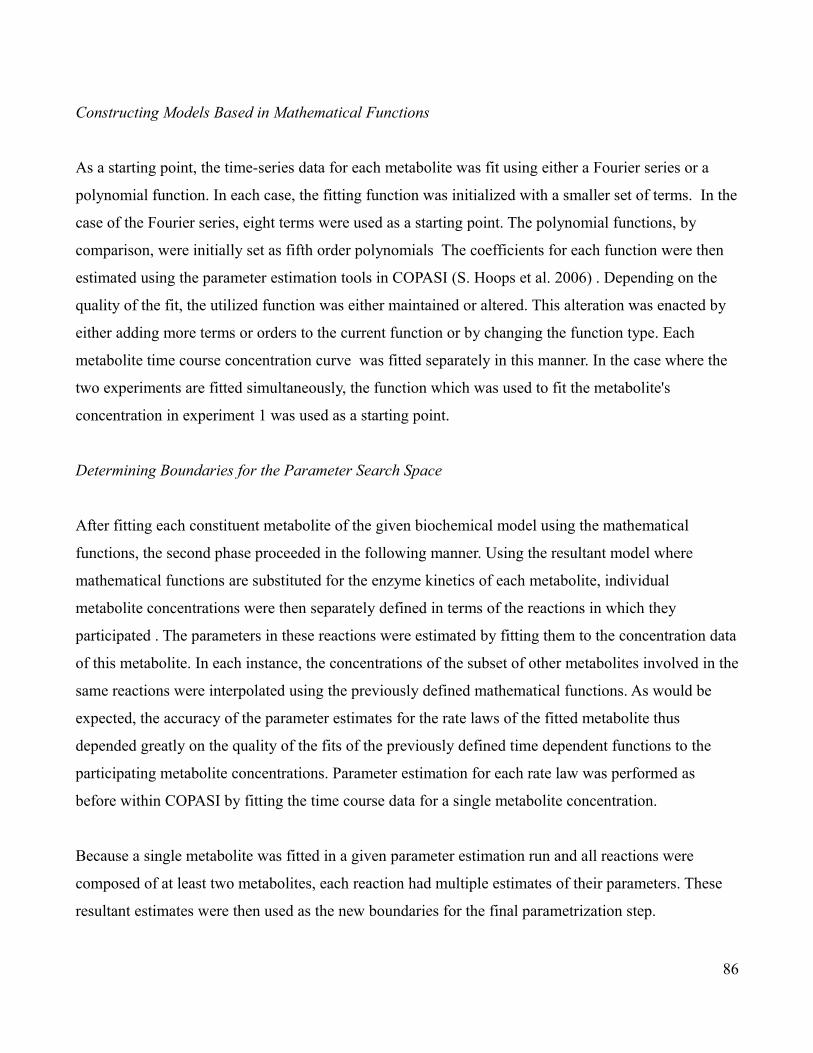
Constructing Models Based in Mathematical Functions

As a starting point, the time-series data for each metabolite was fit using either a Fourier series or a

polynomial function. In each case, the fitting function was initialized with a smaller set of terms. In the

case of the Fourier series, eight terms were used as a starting point. The polynomial functions, by

comparison, were initially set as fifth order polynomials The coefficients for each function were then

estimated using the parameter estimation tools in COPASI (S. Hoops et al. 2006) . Depending on the

quality of the fit, the utilized function was either maintained or altered. This alteration was enacted by

either adding more terms or orders to the current function or by changing the function type. Each

metabolite time course concentration curve was fitted separately in this manner. In the case where the

two experiments are fitted simultaneously, the function which was used to fit the metabolite's

concentration in experiment 1 was used as a starting point.

Determining Boundaries for the Parameter Search Space

After fitting each constituent metabolite of the given biochemical model using the mathematical

functions, the second phase proceeded in the following manner. Using the resultant model where

mathematical functions are substituted for the enzyme kinetics of each metabolite, individual

metabolite concentrations were then separately defined in terms of the reactions in which they

participated . The parameters in these reactions were estimated by fitting them to the concentration data

of this metabolite. In each instance, the concentrations of the subset of other metabolites involved in the

same reactions were interpolated using the previously defined mathematical functions. As would be

expected, the accuracy of the parameter estimates for the rate laws of the fitted metabolite thus

depended greatly on the quality of the fits of the previously defined time dependent functions to the

participating metabolite concentrations. Parameter estimation for each rate law was performed as

before within COPASI by fitting the time course data for a single metabolite concentration.

Because a single metabolite was fitted in a given parameter estimation run and all reactions were

composed of at least two metabolites, each reaction had multiple estimates of their parameters. These

resultant estimates were then used as the new boundaries for the final parametrization step.

86

Final Parametrization

In this step, the kinetic parameters for all of the model's reactions are estimated simultaneously using

the previously determined ranges. The results from both the method where the experiments were fit

simultaneously and where they were fit separately were compared to a version in which the parameter

search space was not limited. The parameter range used in this control was 0 to 2000, and is based

upon the observed parameter range in the BRENDA database (Chang et al. 2009; I. Schomburg et al.

2002). In all cases, both experimental datasets were used as targets for fitting in this final parameter

estimation step.


Parameter estimation at each step was performed using the tool COPASI (S. Hoops et al. 2006).A

discussion of how parameter estimation methods may be performed in COPASI is given by Mendes et

al (Pedro Mendes et al. 2009) . Different optimization algorithms were used at all stages , in the initial

fitting of a metabolite's concentration to a mathematical function, in the fitting of reactions to

individual metabolites, and in the final parameter estimation of the entire model. A description of the

basic stages in the proposed method is given in table 4.2. A summary of the optimization methods used

along with the stages in which they were applied is given in table 4.3.

Table 4.2 The basic stages of the proposed method

Method Stage Description

1 Metabolite concentration fit to function which is only dependent on time

2 ODE for a given metabolite concentration is approximated by using time dependent functions from 1 to substitute for all other

metabolite concentrations in original ODE. These ODEs are fit to the given metabolite concentration within the time course to obtain estimates for the rate equation parameters of reactions in which the

given metabolite participates.

3 Final adjustment of all rate equation parameters is performed using parameter estimates obtained in step 2. Adjustment is performed by

fitting all metabolite concentrations in all available timecourse datasets.

87

Table 4.3: A Brief description of optimization methods used and the method stage in which they were applied

Optimization Method Stages Utilized Brief Description

Particle Swarm All Stochastic method by which a group of particles attempts to find the optimum parameter values by performing multiple,

simultaneous searches over the parameter space

Genetic Algorithm SR All Stochastic tournament selection with parallels genetic selection

Hook & Jeeves 1,2 Direct search method based on previously saved stepwise parameter moves

Levenberg - Marquardt 1,2 Gradient descent which combines Newton's methods with steepest descent


Time Dependent Functions Fit to Simulated Biochemical Data

Time dependent functions, see eqns 4.3 and 4.4, were fit to metabolite concentration data from two

timecourses. In the first timecourse the initial concentration of Glucose is 160 mmol/ml, while in the

second time course the concentration of Glucose was lowered to 75 mmol/ml. The concentrations of

each metabolite within each of these timecourses is fit with a unique function which only depends on

time. Therefore, each metabolite concentration is represented by two functions; one which fits the

metabolite concentration in the first time course and the other which represents the metabolite

concentration within the second time course. At this stage, it is very important that these functions fit

the metabolite concentration time course data as perfectly as possible because all of the later steps in

the method depend on the quality of this fit. In figure 4.2, fits of the time dependent functions to the

concentrations of Fructose, AMP, Triose, and Acetic acid within experiment 1, where the initial

Glucose concentration was 160 mmol/mL, are shown. The concentrations of Fructose and AMP were

fit using a Fourier time series, while the concentrations of Triose and Acetic acid were fit using a

polynomial function.

88

A. B.

C. D.

Figure 4.2 Fits of functions based on either 4.3 or 4.4 to metabolite concentration data. Functions of type 4.4 are used to fit the

concentrations of A. Fructose and B. AMP. Functions of type 4.3 are used to fit the concentrations of C. Acetic acid and D. Triose

Change in Metabolite Concentrations with Respect to Time Using Time Dependent Functions to

Substitute for Interacting Metabolites

In order to separate the initial set of ODEs for the system, such as those in eqn. 4.1, into ODEs which

could be analyzed individually, the interdependence between metabolite concentrations was removed.

These functions, see eqn. 4.5, were made independent by substituting all other metabolite

concentrations with previously determined time dependent functions. These functions were based on

close fits to the given metabolite's concentration time course data. Each of these new ODEs, which

represent the dynamics of an individual metabolite, was fit to the relevant metabolite concentration

89

Fit to AMP C oncentration

-0.2

0

0.2

0.4

0.6

0.8

1

1.2

0100 200 300 400 500 600 700 800 900 100

0

T im e

Conc

entra

tion

in m

mol

/mL

AMP_measuredAMP_fitted

Fit to Acetic acid Concentration

0

50

100

150

200

250

0

100

200

300

400

500

600

700

800

900

1000

T im e

Conc

entra

tion

in m

mol

/mL

Acetic_ac id_measuredAcetic_ac id_fitted

Fit to Triose C oncentration

0102030405060708090

0100 200 300 400 500 600 700 800 900 1000

T i m e

Conc

entra

tion

in m

mol

/mL

Triose_measuredTriose_fitted

Fit to Fructose C oncentration

-10

0

10

20

30

40

50

0100 200 300 400 500 600 700 800 900 100

0

T im e

Conc

entra

tion

in m

mol

/mL

Fru_measuredFru_fitted

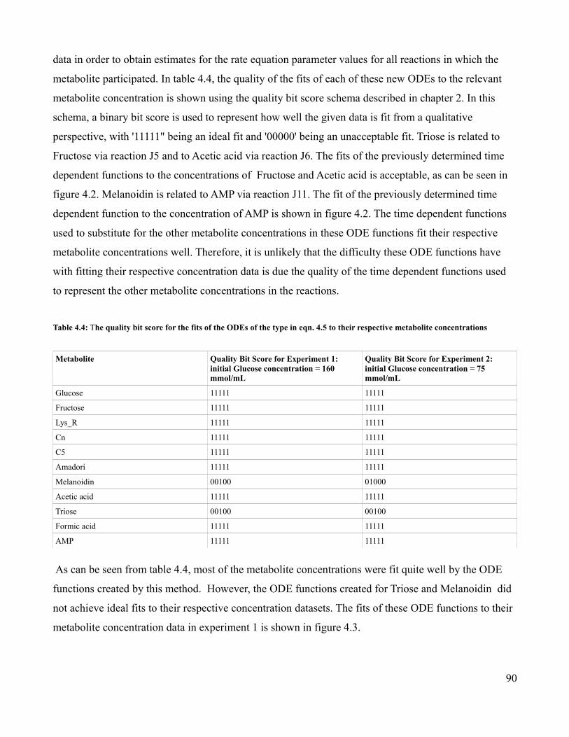
data in order to obtain estimates for the rate equation parameter values for all reactions in which the

metabolite participated. In table 4.4, the quality of the fits of each of these new ODEs to the relevant

metabolite concentration is shown using the quality bit score schema described in chapter 2. In this

schema, a binary bit score is used to represent how well the given data is fit from a qualitative

perspective, with '11111" being an ideal fit and '00000' being an unacceptable fit. Triose is related to

Fructose via reaction J5 and to Acetic acid via reaction J6. The fits of the previously determined time

dependent functions to the concentrations of Fructose and Acetic acid is acceptable, as can be seen in

figure 4.2. Melanoidin is related to AMP via reaction J11. The fit of the previously determined time

dependent function to the concentration of AMP is shown in figure 4.2. The time dependent functions

used to substitute for the other metabolite concentrations in these ODE functions fit their respective

metabolite concentrations well. Therefore, it is unlikely that the difficulty these ODE functions have

with fitting their respective concentration data is due the quality of the time dependent functions used

to represent the other metabolite concentrations in the reactions.

Table 4.4: The quality bit score for the fits of the ODEs of the type in eqn. 4.5 to their respective metabolite concentrations

Metabolite Quality Bit Score for Experiment 1: initial Glucose concentration = 160 mmol/mL

Quality Bit Score for Experiment 2: initial Glucose concentration = 75 mmol/mL

Glucose 11111 11111

Fructose 11111 11111

Lys_R 11111 11111

Cn 11111 11111

C5 11111 11111

Amadori 11111 11111

Melanoidin 00100 01000

Acetic acid 11111 11111

Triose 00100 00100

Formic acid 11111 11111

AMP 11111 11111

As can be seen from table 4.4, most of the metabolite concentrations were fit quite well by the ODE

functions created by this method. However, the ODE functions created for Triose and Melanoidin did

not achieve ideal fits to their respective concentration datasets. The fits of these ODE functions to their

metabolite concentration data in experiment 1 is shown in figure 4.3.

90

A. B.

Figure 4.3: Fits of the ODE functions of the form in Eqn 4.5 to concentration data of A. Triose and B. Melanoidin.

Parameter Ranges Identified Via Proposed Method

In table 4.5, the true values of the kinetic parameters are given. In tables 4.6 and 4.7, the parameter

estimation results obtained by fitting the auxiliary ODE functions, see eq.4.2 , created by the method to

the relevant metabolite concentration data are given.

Table 4.5 The true values for each rate law parameter

Reaction True Parameter Value

J1 1.00E-002

J2 5.09E-003

J3 4.70E-004

J4 1.10E-003

J5 7.12E-003

J6 4.39E-003

J7 1.80E-003

J8 1.11E-001

J9 1.44E-001

J10 1.50E-004

J11 1.25E-001

Table 4.6 : Parameter estimation results from fitting experiment 1 concentration data , where the initial Glucose concentration is

91

F it to T rio s e C o n c e n tra tio n

-100-80-60-40-20

020406080

100

0100 200 300 400 500 600 700 800 900 100

0

T i m e

Conc

entra

tion i

n mmo

l/mL

Trios e_m eas uredTrios e_F it tedM ean_error

F it to M e la n o id in C o n ce n tra tio n

-20

-15

-10

-5

0

5

10

15

20

0100 200 300 400 500 600 700 800 900 1000

T i m e

Conc

entra

tion i

n mmo

l/mL

M elanoid in_m eas uredM elanoid in_ fit tedW eighted_error

160 mmol/L

Reaction Glucose Fructose Acetic

Acid Amadori C5 FormicAcid Cn AMP Melanoidin Lys_R Triose

J1 8.33E-03 1.20E+03

J2 2.96E-165 7.60E+02

J3 3.85E-306 9.88E-04 9.88E-04

J4 5.21E+02 4.13E-03 4.15E-03

J5 3.06E+02 7.50E-03

J6 4.57E-03 4.38E-03 4.55E-03

J7 2.13E-245 1.11E-04 2.13E-62

J8 1.03E-142

7.10E-02 1.15E-01

J9 1.30E-01 2.48E+02

J10 4.01E+02 1.29E-19

8.53E-04

J11 1.11E+02

1.25E-04

Table 4.7 : Parameter estimation results from fitting experiment 2 concentration data, where the initial Glucose concentration is 75 mmol/L are shown

Reaction Glucose Fructose Acetic

Acid Amadori C5 FormicAcid Cn AMP Melanoidi

n Lys_R Triose

J1 9.11E-03 2.00E+03

J2 7.40E-50 3.30E+01

J3 1.68E-46 1.01E-03 4.70E-04

J4 3.43E+02 1.39E-03 1.10E-03

J5 1.76E+02 1.15E-01

J6 4.72E-03 4.38E-03

2.02E-02

J7 4.01E-03 1.78E+00 1.64E-04

J8 8.58E-68 8.03E+02 6.62E-02

J9 1.78E+03 2.72E+02

J10 3.46E+02 0.00E+00

5.73E-303

J11 1.21E+02

5.74E-06

Final Parametrization Results

92

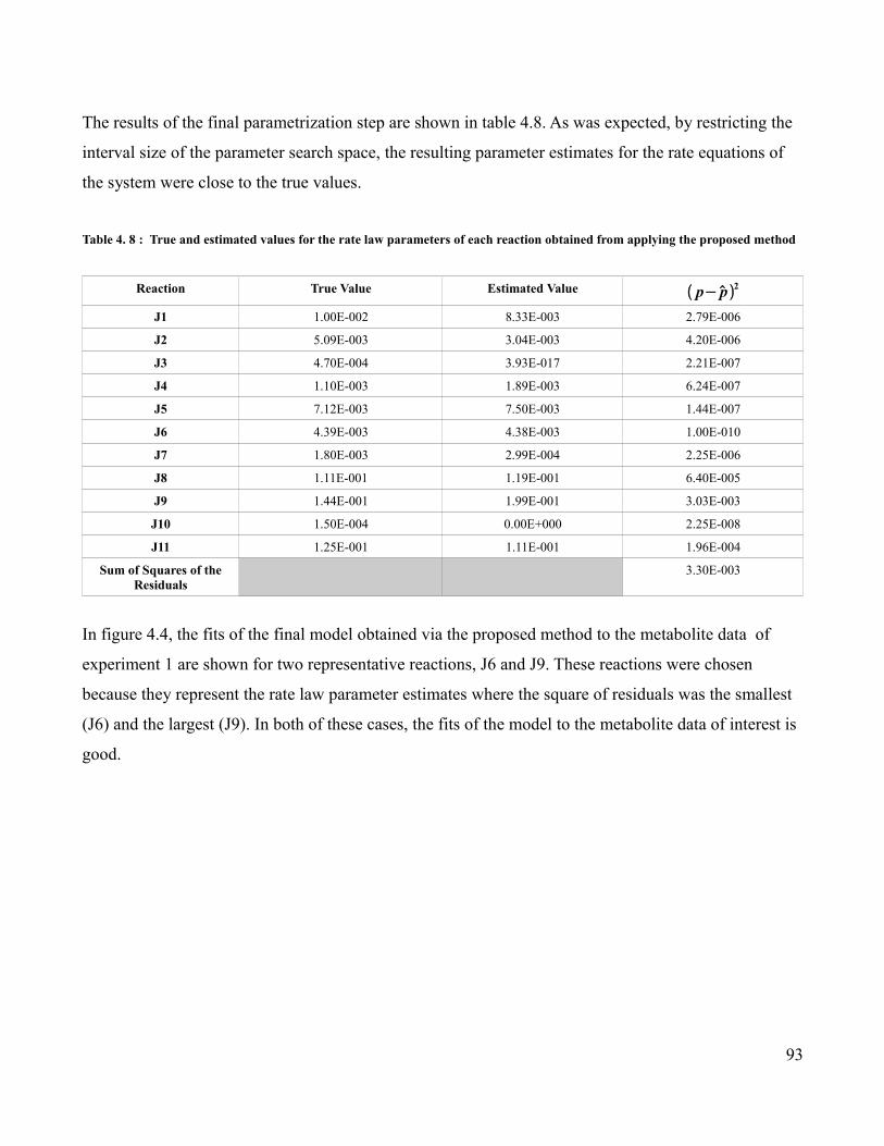
The results of the final parametrization step are shown in table 4.8. As was expected, by restricting the

interval size of the parameter search space, the resulting parameter estimates for the rate equations of

the system were close to the true values.

Table 4. 8 : True and estimated values for the rate law parameters of each reaction obtained from applying the proposed method

Reaction True Value Estimated Value p−p 2

J1 1.00E-002 8.33E-003 2.79E-006

J2 5.09E-003 3.04E-003 4.20E-006

J3 4.70E-004 3.93E-017 2.21E-007

J4 1.10E-003 1.89E-003 6.24E-007

J5 7.12E-003 7.50E-003 1.44E-007

J6 4.39E-003 4.38E-003 1.00E-010

J7 1.80E-003 2.99E-004 2.25E-006

J8 1.11E-001 1.19E-001 6.40E-005

J9 1.44E-001 1.99E-001 3.03E-003

J10 1.50E-004 0.00E+000 2.25E-008

J11 1.25E-001 1.11E-001 1.96E-004

Sum of Squares of the Residuals

3.30E-003

In figure 4.4, the fits of the final model obtained via the proposed method to the metabolite data of

experiment 1 are shown for two representative reactions, J6 and J9. These reactions were chosen

because they represent the rate law parameter estimates where the square of residuals was the smallest

(J6) and the largest (J9). In both of these cases, the fits of the model to the metabolite data of interest is

good.

93

A. B.

Figure 4.4 : The fits of the model, estimated using the proposed method, to the metabolite data for representative reactions are shown for

experiment 1. The fits to : A. J6 and B. J9 are displayed in terms of their constituent metabolites. The parameter range in this instance is

based upon the estimates obtained via the proposed method.

Control Model in Which No Range Boundaries Are Imposed on Final Parameter Estimation

Table 4.9 The true and estimated values for all rate law parameters where no addition range limitations beyond those derived

from BRENDA are imposed

Reaction True Parameter Value Estimated Parameter Value p−p 2

J1 1.00E-002 3.83E+002 1.47E+005

J2 5.09E-003 9.39E-001 8.72E-001

J3 4.70E-004 6.23E+001 3.88E+003

J4 1.10E-003 1.88E-005 1.17E-006

J5 7.12E-003 5.48E-135 5.07E-005

J6 4.39E-003 1.74E+000 3.01E+000

J7 1.80E-003 2.00E+003 4.00E+006

J8 1.11E-001 1.95E+001 3.76E+002

J9 1.44E-001 0.00E+000 2.07E-002

J10 1.50E-004 3.99E-002 1.58E-003

J11 1.25E-001 2.00E+003 4.00E+006

Sum of Squares of the Residuals

8.15E+006

In figure 4.5, plots of the fits of the model obtained using the control method to the metabolite data

94

Reaction J6 Fit Results

0

50

100

150

200

250

010

020

030

040

050

060

070

080

090

010

00

T i m e

Conc

entra

tion

in m

mol

/mL Triose_Measured

Triose_Fitted Acetic_ac id_M eas ured Acetic_ac id_Fitted Cn_Measured Cn_Fitted

Reaction J9 Fit Results

0

0.2

0.4

0.6

0.8

1

1.2

010

020

030

040

050

060

070

080

090

010

00

T im e

Conc

entra

tion

in m

mol

/mL

Amadori_Measured Amadori_Fitted AMP_Measured AMP_Fitted

from experiment 1 are shown for representative reactions, J4 and J11. The estimated parameter value

for the rate law of J4 had the lowest residual square value, while the estimated parameter for J11 had

one of the highest residual square values. The fits for the metabolites which participate in reactions J4

and J11 are not particularly good. However, the fits to the metabolite concentrations in reaction J11

seem better than in J4, even though the parameter value estimated for J11 was much worse than that

estimated for the rate law parameter of J4.

A. B.

Figure 4.5 : The fits of the model, estimated using the control method, to the metabolite data for a representative set of reactions are

shown for experiment 1. The reaction fits: A. J4 and B. J11 are displayed in terms of their constituent metabolites. The parameter range

used in the control method were based upon those obtained from BRENDA.

Conclusions

The method proposed in this chapter demonstrated a strategy by which a system of ODEs, representing

rate laws of a set of interacting metabolites, could be analyzed separately. This was done by

substituting time dependent functions, such as those of eqns. 4.3 or 4.4 , for other metabolite

concentrations not directly represented by the given ODE. The parameter estimates which resulted

from fitting each individual ODE function, see eqn. 4.5, to the concentration data for its respective

metabolite were used to restrict the parameter search space for the original set of ODEs.

The results of applying this method were obtained by using an artificial biochemical network. By using

95

Reaction J4 Results

-100

102030405060708090

010

020

030

040

050

060

070

080

090

010

00

T im e

Conc

entra

tion

in m

mol

/mL

Triose_Measured Triose_Fitted Fru_Measured Fru_Fitted

R eaction J11 F it R esu lts

-202468

10121416

010

020

030

040

050

060

070

080

090

010

00

T i m e

Conc

entra

tion

in m

mol

/mL AMP_Measured

AMP_Fitted Melanoidin_Measured Melanoidin_Fitted

an artificial biochemical network, it was possible to determine the difference between the estimated

values of the rate law parameters, obtained in the proposed and control methods, and the true value of

these parameters. The sum of squares of the residuals between the estimated and true values of

parameters was used to compare the proposed method with the control method.

It was hypothesized that employing this method would have two main benefits over the control

method; improved speed and accuracy. In this study, the sum of squares of the residuals for the

differences in the parameters estimated using the proposed method is much lower than than of the

control sum of squares. The final adjustment step, where parameter estimation is done on the full

system, of the proposed method also took much less time to converge than did the parameter estimation

of the control. Thus, the results of this study support both hypotheses concerning this method. Further

studies should concentrate on different models, to investigate the generality of the method, as well as

data that contains increasing levels of noise to investigate how noise may affect the procedure. In case

it is demonstrated that this is a robust procedure, software could be developed to automate the entire

process.

96

Chapter 5: Conclusions and Future Directions

Introduction

The purpose of this work was to investigate the effect that missing and incomplete knowledge have on

systems biology studies, and to propose methods of accounting for this deficit. Although missing and

incomplete knowledge affects all levels of scientific inquiry, its presence in systems biology is

especially pervasive. A goal of systems biology is to build models which accurately reflect the

underlying complex set of interactions responsible for an organism's ability to respond to

environmental stimuli (Mendes 2001). However, the amount of knowledge necessary to create these

models is generally unavailable. Thus, in many cases systems biology studies must attempt to recover

the whole with only partial information.

Conclusions from Research

The Influence of Partial Network Information on Obtaining System Parameters

The full underlying biochemical network of interactions is generally not known for most organisms. In

chapter 2, an analysis was performed to determine how this incomplete network knowledge might

affect the ability to recover systems level information. Specifically, the focus was on how studying only

the metabolic portion of an artificial biological network might skew the estimations for kinetic

parameters of the studied reactions. It was hypothesized that the rate law parameters for those reactions

which were under greater transcriptional control would be most affected by a study in which only the

metabolome was considered. In order to test this hypothesis, a method was proposed to test the strength

of association between reaction species and pre-identified regulatory components. These regulatory

components were classified as either contributing to metabolic or hierarchical control depending upon

both their identity and the context of their relationship to the metabolic species. For example, in some

contexts a protein was classified as exuding transcriptional control, while in other instances it was

considered an aspect of metabolic control.

97

The results from chapter 2 indicate that under those specific conditions, there were significant

differences overall, as determined by the Wilcoxon signed rank test (Whitley & Ball 2002), between the

true kinetic parameters and those estimated using the only metabolic portion of the Claytor network.

However, the significance of the differences for the most part disappeared when the reactions were

assessed individually. While none of the differences for individual reactions was significant at the α =

0.05 level, one reaction was closer to having significantly different parameter estimates from its true

values than the rest. This reaction was compared to all of the others in terms of its association with

pre-defined transcriptional and metabolic regulatory species. In most of the experiments where the

association with either the transcriptional or metabolic control types for this reaction was assessed, the

association was stronger with the metabolic control type. However, in one experiment, a gene knock

out, this reaction was slightly more associated with the hierarchical control type. Therefore, it was

concluded that the significance of the differences between the true and estimated kinetics were likely

due to the combined effects of non-metabolic regulation on each reaction, rather than on specific

reactions. However, it was noted that a future study should be done to check the association of each

reaction with translational control.

Several observations resulted from calculating the association of each reaction and its component

metabolic species with the metabolic and hierarchical control types. For one, it was observed that the

experiment which was used to calculate kinetic parameter estimates contained the most information.

Here, the amount of information in an experiment refers to the number of metabolic species whose

concentrations underwent alterations due to the experimental conditions. In the other two experiments,

there were several metabolic species whose concentrations were unaffected by the given perturbations.

Because of this lack of information in these experiments, there were several instances where the control

type of a given metabolic species could not be determined. In addition, it was noted that when

association with a control type could be predicted, it was most often predicted as being associated with

metabolic control. These observations indicate that the effect of studying the metabolic reactions in

isolation from transcription and translation will depend on both what the predominant control type of

these reactions is as well as the experimental dataset which is used to estimate the kinetic parameters.

In this study, because most of the reactions were predicted as being predominately under metabolic

control, it is likely that parameters estimated using only the metabolic portion of the network were far

98

less detrimental than in an experiment where hierarchical control was more dominant. It also indicates

that the quality of the parameter estimates determined depends greatly on the amount of information

which can be gleaned from the experiments which they are based upon. If one of the other experiments

had been used to calculate parameter estimates in this study, it is likely that the differences between

these and the true parameter values would be much more significant.

Comparing Methods for Forming General Kinetic Rate laws

Unknown kinetic rate laws are often a confounding factor in constructing accurate models of

biochemical systems. In order to circumvent this lack of knowledge, several methods have been

proposed which can create generalized rate laws. In chapter 3, three of these methods were compared:

generalized mass action (Guldberg & Waage 1879; L. Segel & John J. Tyson 1992), linlog (Visser & J.

J. Heijnen 2003b), and convenience kinetics (Liebermeister & Klipp 2006b). For the purposes of

evaluation, the Claytor artificial biological network was used. The generalized rate law methods were

compared based on how well they managed to fit concentration data from time-series experiments

performed on the Claytor network as well as the number of parameters they employed to obtain this fit.

The criteria for model selection used was the Akaike's Information Criterion (AIC) (Akaike 1974) ,

which takes both of these factors into account. These methods for generalizing rate laws were further

compared based on how sensitive they were to the availability of network knowledge. This sensitivity

was assessed by creating kinetic models by each approach and then estimating the resultant parameter

values when these metabolic reactions were integrated into the full network and then again when these

reactions were separated from the full network. It was expected that convenience kinetics would

perform best overall because the form of its equations is most similar to that of the true kinetic rate

laws. It was further predicted that the generalized mass action kinetics were those who produced the

most accurate results after isolating the metabolic reactions from the full Claytor network .

Surprisingly, the method which performed best in this study was generalized mass action. In fact, when

these methods were implemented on the metabolic portion of the Claytor network isolated from the

transcriptional and translational reactions, the generalized mass action method resulted in a better AIC

value than even the true rate laws. Two possible reasons for this are : 1) generalized mass action has

99

significantly fewer parameters than the other methods 2) certain features of the experimental dataset

made it more amenable to analysis by generalized mass action . The generalized mass action method

did not fit the data quite as well as the true kinetic rate laws, as evidenced by the sum of squares of the

residuals. However, the true kinetic rate laws contain many more parameters than does generalized

mass action. Because the quality of fit for the more complicated model based on the true rate laws is

not significantly better, the simpler model was preferred by AIC. In addition, it is likely that the

experimental dataset being fit was of a type which is more easily fit by generalized mass action. This

experiment was the same as the one used in the study in chapter 2, where it was predicted to be under

predominantly metabolic control. It is possible that generalized mass action was able to fit the data well

because the effects of the modifiers were minimal as compared to the control exerted via metabolism. If

the enzyme concentrations had been altered greatly, via transcriptional regulation, in this experiment,

then it is likely that generalized mass action would not have performed as well.

Convenience kinetics performed essentially the same as the true kinetic rate laws when the metabolic

reactions were separated from the full Claytor network. Thus, convenience kinetics is still likely an

excellent approach for generalizing rate laws when the true kinetic equations are unknown. By contrast,

models based on linlog rate law approximations failed to converge. In two cases, even replacing the

rate laws of a single reaction with linlog caused a failure to converge. This failure indicates that for

these reactions the linlog parameters were unidentifiable, most likely due to certain features of the

equation. Thus, although it has been shown to be effective for the purposes of other studies, linlog was

not not useful in this study.

A Data-Driven Approach to Reducing the Parameter Search Space in Biochemical Systems

In chapter 3, a method is proposed for reducing the parameter search space in biochemical systems. In

the proposed method, the set of ordinary differential equations (ODEs) which represent the kinetic rate

laws of the system are presumed to be known. Calculating estimates for the parameters of systems of

ODEs becomes increasingly difficult as the dimension of the system increases. One way of diminishing

this difficulty would be to somehow estimate the parameter values for the individual ODE functions

separately. In order to accomplish this goal, the equations would need to be made independent from

each other. I proposed a method that accomplishes this aim by using functions which only depended on

100

time; the empirical parameters of these equations have to be estimated from the data, however this is

done very efficiently. These functions were not assumed to contain any structural properties which

related them to the biochemical system, the only requirements were that they fit the concentration time-

course data well and only depend on time – and therefore are decoupled. The functions used in this case

were the polynomial (Durbin 2009) and the truncated Fourier series (Fourier 1888) functions. These

time-dependent functions were used to create auxiliary ODEs, where each ODE function for the

concentration of a given metabolic species was independent from that of every other ODE function in

the model. By employing this method, it was possible to estimate the parameters of each auxiliary

function separately. The resultant values were then used to restrict the interval size of the parameter

search space for the original system of ODEs.

It was hypothesized that this method will greatly improve on the computational time necessary to

obtain estimates for the parameters of the kinetic rate laws of biochemical systems. It was also

proposed that by restricting the search space there would be some scenarios in which the method would

obtain parameter estimates close to the true values, while a global optimization applied to the entire

system with the coupled equations would not obtain accurate values for these parameters, at least not in

a feasible computational time.

The proposed method was tested in a controlled manner by applying it to an artificial biochemical

network obtained from the curated BioModels database (Le Novere et al. 2006). As a control,

parameter estimation was performed on the intact system of ODEs. In this case, the parameter ranges

were bounded to the values existent in the kinetic parameters database BRENDA (I. Schomburg et al.

2002). The control case and the proposed method were compared in terms of how long the final

parameter estimation took and also on how accurate the resulting values were. In both cases, the

proposed method outperformed the control case. Therefore, the hypotheses that the proposed method

would improve on both computation time and accuracy were supported in this study.

101

Future Directions

Simplification

It was mentioned in the introduction to this thesis that in some cases, certain types of missing

information might not be detrimental to the formation of a useful model of the system. This leads to an

interesting possibility for future research. Namely, it may be possible to instead look at the problem of

missing information from a reverse standpoint. By identifying information which is not as necessary

for the formation of the model, it may be possible to simplify a complex model into one which is more

tractable while still describing the known data fairly well. This could be especially useful when

studying large biological networks. It is often difficult to carry out analyzes of these networks because

of their size. In many cases, a researcher will not be interested in the whole network, but only in a

subset of it. By identifying the critical qualities of the network surrounding the subnet of interest, it

may be possible to include only that outside information which is necessary. Ultimately, this non-focal

information could even be substituted by non-mechanistic functions, in a manner similar to how the

concentrations of dependent metabolic species were substituted with time-dependent functions in

Chapter 4. By simplifying the network in this fashion, it may be possible to improve the ease of

analysis for the subnetworks of interest while still including all relevant information.

Integration of 'Omics

In chapter 2, a method was introduced to calculate the association between metabolic species and

potential regulatory species. This method could also be adapted to aid in the integration of different

levels of 'omics data, such as metabolomics and transcriptomics. In spite of the recognition of its

importance, simultaneous study of multiple 'omics levels is still relatively rare. One of the difficulties

involved is ameliorating the discrepancies in scale which can exist between these levels, and in some

cases, within the same level. By employing Z-scores based on correlation, the wide possible differences

in scale would no longer be a confounding issue.

Prediction of Missing Biological Interaction Network Knowledge

102

Another possible future direction indicated by this work is the prediction of pieces of the network

which contain missing information. In chapter 2, the fit of the metabolic model of Claytor network to

the concentration data was imperfect in several cases. The poor fit of a model to the data indicates that

there is missing knowledge of the underlying model. Especially if more data were available, it might be

beneficial in these cases to see if these sub-optimally fit species concentrations were correlated to other

species not codified into the underlying model. In this way, it might be possible to predict both the

location of a gap in information and to suggest relationships which might fill it.

Conclusion

The focus of this work has been to investigate the effect that different types of missing information or

knowledge can have on a systems biology study. Systems biology aims to construct models which take

into account the underlying network of interactions that make it possible for an organism to respond to

its environment. Because of this, much more information is necessary than in a reductionist approach.

Indeed, the amount of information which is required for a systems analysis of an organism is such that

incomplete information is likely to be a consistent reality for these studies. In addition, systems

biological studies must often deal with scenarios where there is incomplete knowledge. Here

knowledge is indicated as separate from information, and refers to information which has been codified

into systems biology models at some level (mechanisms). Missing information and partial knowledge

are interrelated. When information is missing, it is impossible to form models which take this

information into account. Thus, incomplete information leads to incomplete knowledge.

The relationship between hypotheses and experimental studies was discussed in the introduction (Kell

& Oliver 2004). Namely, there is a cyclical association between the formation of valid hypotheses, or

models, of a biological system and experimental evidence. New experimental evidence suggests new

hypotheses, which subsequently suggest new experiments. The relationship between missing

information and incomplete knowledge may be thought of as an aspect of this cycle. Identifying a

situation where there is incomplete information suggests that the underlying knowledge of the system

itself may be incomplete, which suggests the necessity for more experiments. Methods to suggest

which experiments to perform in this situation would be a major advance in the scientific methodology.

103

It is hoped that the results presented in this thesis make a small, but significant, contribution towards

this goal.

104

Bibliography

Akaike, H., 1974. A new look at the statistical model identification. IEEE Transactions in Automatic Control, AC-19, 716-723.

Albeck, J.G. et al., 2008. Modeling a Snap-Action, Variable-Delay Switch Controlling Extrinsic Cell Death. PLoS Biology, 6(12), e299.

Albert, R., 2007. Network Inference, Analysis, and Modeling in Systems Biology. Plant Cell, 19(11), 3327-3338.

Alberts, B. et al., 2007. Molecular Biology of the Cell 5th ed., Garland Science.

Ashyraliyev, M. et al., 2009. Systems biology: parameter estimation for biochemical models. FEBS Journal, 276(4), 902, 886.

Bagheri, N. et al., 2008. Modeling the Drosophila melanogaster Circadian Oscillator via Phase Optimization. J Biol Rhythms, 23(6), 525-537.

Bas Teusink, J.P., 2000. Can yeast glycolysis be understood in terms of in vitro kinetics of the constituent enzymes? Testing biochemistry. European Journal of Biochemistry, 267(17), 5313-5329.

Bertalanffy, L.V., 1973. General System Theory: Foundations, Development, Applications, New York: George Braziller.

Brands, C. & van Boekel, M., 2002. Kinetic modeling of reactions in heated monosaccharide-casein systems. J Agric Food Chem, 50(23).

Broeckling, C.D. et al., 2005. Metabolic profiling of Medicago truncatula cell cultures reveals the effects of biotic and abiotic elicitors on metabolism. J. Exp. Bot., 56(410), 323-336.

Burnham, K. & Anderson, D., 1998. Model Selection and Inference: A Practical Information-Theoretic Approach, Springer-Verlag.

Camacho, D. et al., 2007. Comparison of Reverse-Engineering Methods Using an <i>in Silico</i> Network. Annals of the New York Academy of Sciences, 1115(Reverse Engineering Biological Networks: Opportunities and Challenges in Computational Methods for Pathway Inference), 73-89.

Camacho, D., de la Fuente, A. & Mendes, P., 2005. The origin of correlations in metabolomics data. Metabolomics, 1(1), 53-63.

Caspi, R. et al., 2006. MetaCyc: a multiorganism database of metabolic pathways and enzymes. Nucl. Acids Res., 34(suppl_1), D511-516.

105

Chang, A. et al., 2009. BRENDA, AMENDA and FRENDA the enzyme information system: new content and tools in 2009. Nucl. Acids Res., 37(Database isse), D588-D592.

Chen, W.W. et al., 2009. Input-output behavior of ErbB signaling pathways as revealed by a mass action model trained against dynamic data. Mol Syst Biol, 5(239), 1-19.

Cleland, W.W., 1963. The kinetics of enzyme-catalyzed reactions with two or more substrates or products. I. Nomenclature and rate equations. Biochimica et biophysica acta, 67, 104.

Clerc, M. & Kennedy, J., 2002. The Particle Swarm-Explosion, Stability, and Convergence in a Multidimensional Complex Space. IEEE Transactions on Evolutionary Computation, 6, 58-73.

Cook, P. & Cleland, W., 2007. Enzyme Kinetics and Mechanism 1st ed., Madison Ave, New York, NY: Taylor & Francis Group, LLC.

Cooley, J. & Tukey, J., 1965. An algorithm for the machine calculation of complex Fourier series. Math. Comput., 19, 297-301.

Cornish-Bowden, A., An automatic method for deriving steady-state rate equations. Biochem. J., 165, 55-59.

Deane, C.M. et al., 2002. Protein Interactions: Two Methods for Assessment of the Reliability of High Throughput Observations. Mol Cell Proteomics, 1(5), 349-356.

Draeger, A. et al., 2009. Modeling metabolic networks in C. glutamicum: a comparisonof rate laws in combination with various parameter optimizationstrategies. BMC Systems Biology, 3(1), 5.

Drager, A. & Kronfeld, M., 2007. Benchmarking Evolutionary Algorithms on Convenience Kinetics Models of the Valine and Leucine Biosynthesis in C. glutamicum. IEEE Congress on Evolutionary Computation.

Drager, A. et al., 2008. SBMLsqueezer: A CellDesigner plug-in to generate kinetic rate equations for biochemical networks. BMC Systems Biology, 2(1), 39.

Durbin, J.R., 2009. Modern Algebra: An Introduction, Hoboken, N.J.: John Wiley & Sons.

Eubank, R.L. & Speckman, P., 1990. Curve fitting by polynomial-trigonometric regression. Biometrika, 77(1), 1-9.

Famili, I., Mahadevan, R. & Palsson, B.O., 2005. k-Cone Analysis: Determining All Candidate Values for Kinetic Parameters on a Network Scale. , 88(3), 1616-1625.

Fisher, R.A., 1935. The Logic of Inductive Inference. Journal of the Royal Statistical Society, 98(1), 39-82.

106

Fisher, R., 1992. On the mathematical foundations of Theretical Statistics. In Breakthroughs in Statistics Volume I. Springer Series in Statistics. New York: Springer-Verlag, pp. 11-44.

Fourier, J., 1888. Oeuvres de Fourier Gauthier-Villars, ed., Les Soins de. M. Gaston Darboux; Ministere de l'Instruction.

de la Fuente, A. et al., 2002. Metabolic control in integrated biochemical systems. Eur J Biochem, 269(18), 4408, 4399.

Funahashi, A. et al., 2008. CellDesigner 3.5: A Versatile Modeling Tool for Biochemical Networks. Proceedings of the IEEE, 96(8), 1254-1265.

Funahashi, A. et al., 2003. CellDesigner: a process diagram editor for gene-regulatory and biochemical networks. BIOSILICO, 1, 159-162.

Giersch, C., 1994. Determining Elasticities from Multiple Measurements of Steady-State Flux Rates and Metabolite Concentrations - Theory. Journal of Theoretical Biology, 169, 89 - 99.

Giersch, C. & CornishBowden, A., 1996. Extending double modulation: Combinatorial rules for identifying the modulations necessary for determining elasticities in metabolic pathways. Journal of Theoretical Biology, 182, 361 - 369.

Gillespie, D.T., 2000. The chemical Langevin equation. The Journal of Chemical Physics, 113(1), 297-306.

Goldberg, D., 1989. Genetic Algorithms in Search, Optimization, and Machine Learning, Reading, MA: Wesley Publishing Company, Inc.

Guldberg, C. & Waage, P., 1879. Uber die chemische Affinitat. J. Prakt. Chem., 19(69).

Guy, C. et al., 2008. Metabolomics of temperature stress. Physiologia Plantarum, 132(2), 220-235.

Hall, P., Marron, J. & Neeman, A., Geometric representation of high dimension,low sample size data. Journal of the Royal Statistical Society B, 67(3), 427-444.

Heinrich, R. & Schuster, S., 1996. The regulation of cellular systems, New York: Chapman & Hall.

Henri, V., 1903. Lois generales de l'Action des Diastases., Paris: A. Hermann.

Hoops, S. et al., 2006. COPASI--a COmplex PAthway SImulator. Bioinformatics, 22(24), 3067-3074.

Iyengar, R. & Bhalla, U., 1999. Emergent properties of networks of biological signaling pathways. Science, 283(5400), 381-388.

Kacser, H. & Burns, J.A., 1979. MOlecular democracy: who shares the controls? Biochem Soc Trans, 7, 1149 - 1160.

107

Kacser, H. & Burns, J., 1995. The Control of Flux: 21 Years on. Biochemical Society Transactions, 23, 341-366.

Kaern, M. et al., 2005. Stochasticity in gene expression: from theories to phenotypes. Nat Rev Genet, 6(6), 451-464.

Kanehisa, M. & Goto, S., 2000. KEGG: Kyoto Encyclopedia of Genes and Genomes. Nucl. Acids Res., 28(1), 27-30.

Kanehisa, M. et al., 2006. From genomics to chemical genomics: new developments in KEGG. Nucl. Acids Res., 34(suppl_1), D354-357.

Kaneko, K., 2006. Life: An Introduction to Complex Systems Biology, Berlin Heidelberg New York: Springer-Verlag.

Kell, D.B. & Oliver, S.G., 2004. Here is the evidence, now what is the hypothesis? The complementary roles of inductive and hypothesis-driven science in the post-genomic era. BioEssays, 26(1), 99-105.

Kendall, M., 1938. A New Measure of Rank Correlation. Biometrika, 30, 81-89.

Kendall, M., 1975. Rank Correlation Methods, London: Griffin.

Kennedy, J. & Eberhart, R., 1995. Particle swarm optimization. Proc. of the IEEE Int. Conf. on Neural Networks, 1942-1948.

King, E. & Altman, C., 1956. "A Schematic Method of Deriving the Rate Laws for Enzyme-Catalyzed Reactions. J. Phys. Chem., 60, 1375-1378.

Kitano, H., 2002. Systems Biology: A Brief Overview. Science, 295(5560), 1662-1664.

Klipp, E. et al., 2005a. Enzyme Kinetics and Thermodynamics. In Systems Biology in Practice. Concepts, Implementation, amd Application. KGaA, Weinheim: Wiley-VCH Verlag GmbH & Co., pp. 140-156.

Klipp, E. et al., 2005b. Systems Biology in Practice. Concepts, Implementation, amd Application. 1st ed., KGaA, Weinheim: Wiley-VCH Verlag GmbH & Co.

Kotte, O. & Heinemann, M., 2009. A divide-and-conquer approach to analyze underdetermined biochemical models. Bioinformatics, 25(4), 519-525.

Krohs, U. & Callebaut, W., 2007. Data without models merging with models without data. In Systems Biology Philosophical Foundations. Amsterdam, The Netherlands: Elsevier, pp. 181-209.

ter Kuile, B.H. & Westerhoff, H.V., 2001. Transcriptome meets metabolome: hierarchical and metabolic regulation of the glycolytic pathway. FEBS Lett, 500, 169 - 171.

108

Le Novere, N. et al., 2006. BioModels Database: a free, centralized database of curated, published, quantitative kinetic models of biochemical and cellular systems. Nucl. Acids Res., 34(suppl_1), D689-691.

Liebermeister, W. & Klipp, E., 2006a. Bringing metabolic networks to life: convenience rate law and thermodynamic constraints. Theor Biol Med Model, 3, 41.

Liebermeister, W. & Klipp, E., 2006b. Bringing metabolic networks to life: integration of kinetic, metabolic, and proteomic data. Theor Biol Med Model, 3, 42.

McDonald, J., 2008. Handbook of Biological Statistics, Baltimore, Maryland: Sparky House Publishing. Available at: http://udel.edu/~mcdonald/statintro.html.

McGee, V.E. & Carleton, W.T., 1970. Piecewise Regression. Journal of the American Statistical Association, 65(331), 1109-1124.

van der Meer, R., Westerhoff, H. & Van Dam, K., 1980. Linear relation between rate and thermodynamic force in enzyme-catalyzed reactions. Biochimica et Biophysica Acta (BBA) - Bioenergetics, 591(2), 488-493.

Mendes, 2001. Modeling Large Biological Systems From Functional Genomic Data: Parameter Estimation. In Kitano, ed. Foundations of Systems Biology. Cambridge, Massachusetts: The MIT Press, pp. 162-186.

Mendes, P., Kell, D.B. & Westerhoff, H.V., 1992. Channelling can decrease pool size. Eur J Biochem, 204, 257-266.

Mendes, P., Sha, W. & Ye, K., 2003. Artificial gene networks for objective comparison of analysis algorithms. Bioinformatics(Oxford,England), 19(90002), 122ii.

Mendes, P. et al., 2009. Computational Modeling of Biochemical Networks Using COPASI. In Methods in Molecular Biology. Springer-Verlag, pp. 17-59.

Mendes, P. & Kell, D., 1998. Non-linear optimization of biochemical pathways: applications to metabolic engineering and parameter estimation. Bioinformatics, 14(10), 869-883.

Michaelis, L. & Menten, M., 1913. Die Kinetik der Invertinwirkung. Biochemische Zeitschrift, 49, 333-369.

Minton, A., 2006. How can biochemical reactions within cells differ from those in test tubes? J Cell Sci, 119, 2863-2869.

Moco, S., Schneider, B. & Vervoort, J., 2009. Plant Micrometabolomics: The Analysis of Endogenous Metabolites Present in a Plant Cell or Tissue. Journal of Proteome Research, 8(4), 1694-1703.

Moles, C.G., Mendes, P. & Banga, J.R., 2003. Parameter Estimation in Biochemical Pathways: A Comparison of Global Optimization Methods. Genome Res, 13, 2467 - 2474.

109

Noble, D., 2002. The rise of computational biology. Nat Rev Mol Cell Biol, 3(6), 459-463.

Onsager, L., 1931. Reciprocal Relations in Irreversible Processes. I. Physics Review, 37(4), 405-426.

Pekar, M., 2007. Affinity and Reaction Rates: Reconsideration of Experimental Data. Helvetica Chimica Acta, 90, 1897-1916.

Polisetty, P., Voit, E. & Gatzke, E., 2006. Identification of metabolic system parameters using global optimization methods. Theoretical Biology and Medical Modelling, 3(1), 4.

R Development Core Team, 2009. R: A language and environment for statistical computing, Vienna, Austria: R Foundation for Statistical Computing. Available at: http://www.R-project.org.

Reeves, G. & Fraser, S., 2009. Biological Systems from an Engineer's Point of View. PLoS Biology, 7(1).

van Riel, N.A.W., 2006. Dynamic modelling and analysis of biochemical networks: mechanism-based models and model-based experiments. Brief Bioinform, 7(4), 364-374.

Rizzi, M. et al., 1997. In vivo analysis of metabolic dynamics in Saccharomyces cerevisiae .2. Mathematical model. Biotechnology and Bioengineering, 55, 592 - 608.

Rosen, R., 1985. Anticipatory Systems: Philosophical, Mathematical & Methodological Foundations 1st ed., Elmsford, New York: Pergamon Press Inc.

Rosen, R., 1991. Life Itself., Columbia University Press.

Rottenberg, H., 1973. The Thermodynamic Description of Enzyme-Catalyzed Reactions: The Linear Relation between the Reaction Rate and the Affinity. Biophysical Journal, 13(6), 503-511.

Runarsson, T. & Yao, X., 2000. Stochastic ranking for constrained evolutionary optimization. IEEE Transactions on Evolutionary Computation, 4, 284-294.

Sabouri-Ghomi, M. et al., 2007. Antagonism and bistability in protein interaction networks. Journal of Theoretical Biology, 250(1), 209-218.

Sahle, S. et al., 2008. A new strategy for assessing sensitivities in biochemical models. Philos Transact A Math Phys Eng Sci., 366(1880):3619-31.

Schmitt, L.M. & Droste, S., 2006. Convergence to global optima for genetic programming systems with dynamically scaled operators. In Proceedings of the 8th annual conference on Genetic and evolutionary computation. Seattle, Washington, USA: ACM, pp. 879-886.

Schomburg, I., Chang, A. & Schomburg, D., 2002. BRENDA, enzyme data and metabolic information. Nucl Acids Res, 30, 47 - 49.

110

Segel, I., 1975. Enzyme Kinetics, New York: John Wiley.

Segel, L. & Tyson, J.J., 1992. Law of mass action. Nature, 357(6374), 106.

Smallbone, K. et al., 2007. Something from nothing: bridging the gap between constraint-based and kinetic modelling. FEBS J, 274(21), 5576-85.

Stark, J., Callard, R. & Hubank, M., 2003. From the top down: towards a predictive biology of signalling networks . Trends in Biotechnology, 21(7), 290-293.

Steuer, R. et al., 2006. Structural kinetic modeling of metabolic networks. Proc Natl Acad Sci U S A, 103(32), 11868-73.

Stolovitzky, G., Monroe, D. & Califano, A., 2007. Dialogue on Reverse-Engineering Assessment and Methods: The DREAM of High-Throughput Pathway Inference. Annals of the New York Academy of Sciences, 1115, 11-22.

Stolovitzky, G., Prill, R. & Califano, A., 2009. Lessons from the DREAM2 Challenges. Annals of the New York Academy of Sciences, 1158, 159-95.

Teusink, B. et al., 2000. Can yeast glycolysis be understood in terms of in vitro kinetics of the constituent enzymes? Testing biochemistry. European Journal of Biochemistry, 267, 5313 - 5329.

Valz, P.D. & Thompson, M.E., 1994. Exact Inference for Kendall's S and Spearman's ρ with Extension to Fisher's Exact Test in r x c Contingency Tables. Journal of Computational and Graphical Statistics, 3(4), 459-472.

Vaseghi, S. et al., 1999. In vivo dynamics of the pentose phosphate pathway in Saccharomyces cerevisiae. Metab Eng, 1, 128 - 140.

Visser, D. & Heijnen, J.J., 2003a. Dynamic simulation and metabolic re-design of a branched pathway using linlog kinetics. Metab Eng, 5(3), 164-76.

Visser, D. & Heijnen, J.J., 2003b. Dynamic simulation and metabolic re-design of a branched pathway using linlog kinetics. Metabolic Engineering, 5, 164 - 176.

Visser, D. et al., 2004. Optimal re-design of primary metabolism in Escherichia coli using linlog kinetics. Metab Eng, 6(4), 378-90.

Voit, E.O., 1992. Optimization in integrated biochemical systems. Biotechnology and Bioengineering, 40(5), 572-582.

Weir, B., 1993. Genetic Data Analysis II. Sunderland, MA: Sinauer Associates, Inc. pp. 133-135.

Westerhoff, H. & Kahn, D., 1993. Control involving metabolism and gene expression. Acta

111

Biotheoretica, 41, 75-83.

Wheeler, B., SuppDists: Supplementary distributions, Available at: http://CRAN.R-project.org/package=SuppDists.

Whitley, E. & Ball, J., 2002. Statistics review 6: Nonparametric methods. Crit Care, 6(6), 509-513.

Wimsatt, W., 2007. On building reliable pictures with unreliable data: An evolutionary and developmental coda for the new systems biology. In Systems Biology Philosophical Foundations. Amsterdam, The Netherlands: Elsevier, pp. 103-120.

Wolkenhauer, O. & Ullah, M., 2007. All models are wrong... some more than others. In Systems Biology Philosophical Foundations. Amsterdam, The Netherlands: Elsevier, pp. 163-179.

Wright, B. & Kelly, P., 1981. Kinetic models of metabolism in intact cells, tissues, and organisms. Curr. Top. Cell., 19, 103-158.

Wu, L. et al., 2004. A new framework for the estimation of control parameters in metabolic pathways using lin-log kinetics. European Journal of Biochemistry, 271(16), 3348-3359.

Zhao, J. et al., 2008. Extraction of elementary rate constants from global network analysis of E. coli central metabolism. BMC Systems Biology, 2(1), 41.

112

Documents

Systems Biology in an Imperfect World: Modeling Biological ...Systems Biology in an Imperfect World: Modeling Biological Systems with Incomplete Information Revonda M. Pokrzywa ABSTRACT