Systematic Risk∗

Ohad Kadan† Fang Liu‡ Suying Liu§

October 2013

Abstract

The systematic risk of an asset represents the contribution of the asset to thetotal risk of a portfolio. In this paper we study systematic risk in a setting thatallows risk to capture a variety of attributes such as high distribution momentsand rare disasters. We offer two different approaches. First is an axiomaticapproach in which we specify desirable properties of a systematic risk measure,resulting in a unique solution to the problem. Second is an equilibrium frameworkgeneralizing the Capital Asset Pricing Model (CAPM) to allow for a broad setof risk attributes. The equilibrium approach generalizes classic results includingthe two fund separation theorem, the effi ciency of the market portfolio, andthe security market line. Both approaches lead to the same result in whichsystematic risk is measured by a scaled version of the Aumann-Shapley (1974)diagonal formula. In the special case where the only risk aspect of interest is thevariance, our systematic risk measure coincides with the traditional beta.

1 Introduction

Risk is a complex concept. The definition of risk and its implications have longbeen the subject of both academic and practical debate. This issue has gained evenmore prominence during the recent financial crisis, when markets and individualassets were hit by catastrophic events whose ex-ante probabilities were considerednegligible. Indeed, these events demonstrate that “risk” accounts for much morethan what is measured by the variance of the returns of an asset. High distributionmoments, rare disasters, and downside risk are just some of the different aspects thatmay be of interest when measuring risk.

In this paper we allow “risk” to take a very general form. We then re-visit theclassic question of how to “fairly”allocate total portfolio risk among different assets inthe portfolio. Such a “fair”allocation should reflect the contribution of an asset to therisk of the portfolio, which is often termed “systematic risk.”Traditional measures of

∗We thank Phil Dybvig and Sergiu Hart as well as seminar participants at Cornell University, He-brew University, Hong Kong Polytechnic University, Indiana University, University of Pennsylvania,and Washington University in St. Louis for helpful comments and suggestions.†Olin Business School, Washington University in St. Louis. E-mail: kadan@wustl.edu.‡Olin Business School, Washington University in St. Louis. E-mail: fliu23@wustl.edu.§Olin Business School, Washington University in St. Louis. E-mail: sliua@wustl.edu.

1

systematic risk focus on a narrow set of risk attributes. In particular, the most well-known and widely used measure of systematic risk is the “beta”of the asset, whichis the slope from regressing the asset returns on portfolio returns (Sharpe (1964),Lintner (1965a,b), and Mossin (1966)). Beta is the contribution of an asset to therisk of the portfolio as measured by the variance of its return. It is a fundamentalconcept in financial economics which sets the foundations to all risk-return analysisas part of the Capital Asset Pricing Model (CAPM). However, the traditional betaignores all aspects of risk other than the variance such as high distribution momentsand rare disasters.

We offer two different approaches to the risk allocation problem. First is an ax-iomatic approach in which we specify desirable properties of a systematic risk measurewhich lead to a unique solution to the problem. Second, we study an equilibriumframework generalizing the traditional CAPM to allow for a broad set of risk at-tributes. The equilibrium approach allows us to generalize classic results such as thetwo fund separation theorem, the effi ciency of the market portfolio, and the securitymarket line. Both approaches lead to the same result in which systematic risk ismeasured by a scaled version of the Aumann-Shapley (1974) diagonal formula, whichwas developed as a tool to fairly allocate cost or surplus among players in cooperativegames. In the special case where the only risk aspect of interest is the variance, oursystematic risk measure coincides with the traditional CAPM beta.

We begin with a broad definition of what would constitute a measure of risk. Wedefine a risk measure as any mapping from random variables to real numbers. Thatis, a risk measure is simply a summary statistic that encapsulates the randomnessusing just one number. The variance (or standard deviation) is obviously the mostcommonly used risk measure. However, many other risk measures have been proposedand used. For example, high distribution moments can account for skewness and tailrisk, downside risk accounts for the variation in losses, and value-at-risk is a popularmeasure of disaster risk. Recently, Aumann and Serrano (2008) and Foster and Hart(2009) offered two appealing risk measures that account for all distribution momentsand for disaster risk.1 All of these measures fall under our wide umbrella of riskmeasures. Moreover, any linear combination of risk measures is itself a risk measure.Thus, one can easily create measures of risk that account for a number of dimensionsof riskiness, assigning the required weight to each dimension.

Many cases of interest involve measuring the contribution of one asset to the riskof a portfolio of assets. For example, the asset pricing literature has tied the returnof a financial asset to the return of the market through “beta,”which is a measure ofthe contribution of the asset to the variance of the market portfolio. Similarly, it maybe desirable to estimate the contribution of banks and other financial institutions tothe total market risk (known as systemic risk). Banks and other financial institutionsmay also find it useful to calculate the contribution of different assets on their balancesheet to the total risk of the institution, so that each asset or business unit could be“taxed”appropriately. All of these problems are essentially risk allocation problems

1See Hart (2011) for a unified treatment of these two measures and Kadan and Liu (2013) for ananalysis of the moment properties of these measures.

2

in which total risk should be allocated among the constituents of a portfolio.We first tackle this problem from an axiomatic point of view. We state four

economically plausible properties that risk allocation measures are expected to satisfy.These properties are:

• Normalization. The weighted average of the systematic risk across all assets ina portfolio is normalized to 1. This implies that assets with high contribution tototal risk have systematic risk higher than 1, while assets with low contributionhave systematic risk lower than 1.

• Linearity. If a risk measure is the sum of two other risk measures, then thesystematic risk of each asset is a linear transformation of the systematic risksunder the individual risk measures.

• Proportionality. We broaden the notion of “perfect correlation”to arbitrary riskmeasures. We then ask that if assets are perfectly correlated in the appropriatesense, then their systematic risks are proportionally related.

• Monotonicity. We broaden the notion of “positive correlation”to arbitrary riskmeasures. We then ask that if all assets in the portfolio are positively correlatedin the appropriate sense, then their systematic risks are non-negative.

We show that there is a unique systematic risk measure that satisfies these fourproperties. This measure is given by a scaled version of the Aumann-Shapley (1974)diagonal formula. Essentially, this formula calculates for each asset the average ofits marginal contributions to portfolios along a diagonal starting from the origin andending at the portfolio of interest. In the common case where the risk measure ishomogenous of some degree, our solution becomes very simple, assigning to each assetits marginal contribution to portfolio risk scaled by the weighted average of marginalcontributions of all assets. The proof of the axiomatization result relies on a mappingbetween risk allocation problems to the cost allocation problems studied in Billeraand Heath (1982).

Our systematic risk measure is easy to calculate for a variety of risk measures usingsimple calculus methods. Importantly, when risk is measured using “variance,”ourmeasure boils down to the familiar beta. More generally, we show how our systematicrisk measure can be calculated in closed form for various risk measures accountingfor high distribution moments, rare disasters as well as other risk attributes.

Our next step is to show that our measure of systematic risk arises naturally in anequilibrium model generalizing the CAPM to a broad set of risk measures. The ideais simple. In the classic CAPM setting investors are assumed to have mean-variancepreferences. That is, their utility is increasing in the expected payoff and decreasingin the variance of their payoffs. In our generalized setting we assume that investorshave mean-risk preferences, where the term “risk”stands for a host of potential riskmeasures. We provide mild suffi cient conditions under which these preferences arelocally consistent with expected utility in the sense of Machina (1982).

3

We consider an exchange economy with a finite number of risky assets, one risk-free asset, and a finite number of investors with mean-risk preferences. As usual, inequilibrium each investor chooses a portfolio of assets from the set of effi cient port-folios, minimizing risk for a given expected return. However, due to the generality ofthe risk measure, the geometry of this set is more complicated than in the case whererisk is measured by the variance. Nevertheless, we establish suffi cient conditions un-der which the solution to each investor’s problem satisfies Tobin’s (1958) two-fundmoney separation property. That is, each investor’s optimal portfolio of assets can bepresented as a linear combination of the risk-free asset and a unique portfolio of riskyassets. The suffi cient conditions we propose consist of the following three propertiesof risk measures:

• Convexity. The risk of a portfolio of assets (with a positive weight assignedto each asset) is smaller than the corresponding weighted average risk of theconstituent assets.

• Homogeneity. Scaling up a random investment by a factor t > 0 increases riskby a factor of tk for some k.

• Risk-free property. Assets paying a constant amount are the least risky assets,and adding a risk-free asset to a risky asset does not affect total risk.

We demonstrate that many risk measures satisfy these suffi cient conditions, wherethe variance is just one special case. A consequence of two-fund money separationis that the equilibrium market portfolio lies on the effi cient frontier. Using this, andunder a smoothness condition we establish a generalization of the classic securitymarket line (SML) to a large class of risk measures. Specifically, in equilibrium, theexpected return of each risky asset i satisfies

E (zi) = rf + Bi(E(zM)− rf

),

where zi is the risky return of asset i, zM is the risky return of the market portfolio,rf is the risk-free rate, and Bi is our measure of systematic risk. Thus, our measureof systematic risk emerges naturally in an equilibrium setting as a generalization ofbeta. In particular, in equilibrium, each asset’s expected return reflects its marginalcontribution to the total risk (broadly defined) of the market portfolio.

Our paper contributes to several strands of the literature. First, the paper addsto the growing literature on risk measurement. This literature dates back to Hadarand Russell (1969), Hanoch and Levy (1969), and Rothschild and Stiglitz (1970) whoextend the notion of riskiness beyond the “variance”framework by introducing sto-chastic dominance rules. Artzner, Delbaen, Eber, and Heath (1999) specify desirableproperties of coherent risk measures. More recently Aumann and Serrano (2008),Foster and Hart (2009, 2013), and Hart (2011) came up with appealing risk mea-sures that generalize conventional stochastic-dominance rules. Notably, all the riskmeasures discussed in this literature are idiosyncratic in nature. Our paper adds tothis literature by specifying a method to calculate the systematic risk of an asset for

4

any given risk measure. This in turn allows us to study the fundamental risk-returntrade-off associated with a risk measure.

Our paper also adds to the recent literature on the measurement of systemic risk,which is the risk that the entire economic system collapses. Adrian and Brunnermeier(2008) define the ∆CoV aR measure as the difference between the value-at-risk of thebanking system conditional on the distress of a particular bank and the value-at-risk ofthe banking system given that the bank is solvent. Acharya, Pedersen, Philippon, andRichardson (2010) propose the Systemic Expected Shortfall measure (SES), whichestimates the exposure of a particular bank in terms of under-capitalization to asystemic crisis. Our paper takes a general approach to the problem of estimatingthe contribution of one asset to the risk of a portfolio of assets. We rely on bothan axiomatic approach and an equilibrium framework to provide an easy-to-calculateand intuitive measure that applies to a wide variety of risk measures, as well as in anarray of contexts.

The paper also contributes to the growing literature on high distribution momentsand disaster risk and their effect on prices. Kraus and Litzenberger (1976), Jean(1971), Kane (1982), and Harvey and Siddique (2000) argue that investors favorright-skewness of returns, and demonstrate the cross-sectional implications of thiseffect. In addition, Barro (2006, 2009), Gabaix (2008, 2012), Gourio (2012), Chen,Joslin, and Tran (2012), and Wachter (2013) study the aversion of investors to tail riskand rare disasters. Our paper adds to this literature by outlining a general measure ofsystematic risk that can capture the contribution of an asset to a range of market riskaspects such as high distribution moments, rare disasters, and downside risk. Ourmeasure applies to homogeneous and non-homogeneous risk measures, and can becalculated easily when one needs to estimate the contribution of a particular asset tothe risk of a portfolio. Our approach to equilibrium essentially follows a reduced form,where preferences are described through the aversion to broadly defined risk. It shouldbe emphasized, however, that our approach is stylized and does not account for thedynamics of returns, cash flows and consumption as do modern consumption basedasset pricing models (e.g., Bansal and Yaorn (2004) and Campbell and Cochrane(1999)). These models rely on the specification of a utility function (such as Epsteinand Zin (1989) preferences or preferences reflecting past habits). One advantage ofour approach is that it provides a very parsimonious and simple one factor modelthat can capture different aspects of risk in a manner that may lend itself naturallyto empirical investigation.

Additionally, the paper adds to an extensive list of studies applying the Aumann-Shapley solution concept in different contexts. For example, Billera, Heath, andRaanan (1978) solve a telephone billing allocation problem, Samet, Tauman, andZang (1984) solve a transportation costs allocation problem, and Powers (2007) stud-ies the allocation of insurance risk. Billera, Heath, and Verrecchia (1981) use a relatedprocedure to allocate production costs. Finally, Tarashev, Borio, and Tsatsaronis(2010) use the Shapley value (Shapley (1953), a discrete version of the Aumann-Shapley solution concept) to measure systemic risk. Our paper offers theoreticalfoundations for their practical approach.

5

The paper proceeds as follows. In Section 2 we define the notion of risk measures.Section 3 presents the axiomatic approach to the risk allocation problem. In Section4 we study the equilibrium setup and offer a generalization of the CAPM. Section 5concludes. Technical proofs are in Appendix I, and additional technical results areprovided in Appendices II and III.

2 Risk Measures

Let (Ω,F , P ) be a probability space, where Ω is the state space, F is the σ-algebra ofevents, and P (·) is a probability measure. As usual, a random variable is a measurablefunction from Ω to the reals. In the context of investments, we typically considerrandom variables representing the payoffs or the returns of financial assets. Thus, weoften refer to random variables as “investments”or “random returns.”We genericallydenote random variables by z, which is a shorthanded notation for z (ω) ∀ω ∈ Ω. Werestrict attention to random variables for which all moments exist. We denote theexpected value of z by E (z) and its kth central moment by mk (z) = E (z − E (z))k,where k ≥ 2.

A risk measure is simply a function that assigns to each random variable a singlenumber summarizing its riskiness. Formally,

Definition 1 A risk measure is a function mapping random variables to the reals.

We generically denote risk measures by R (·) . The simplest and most commonlyused risk measure is the the variance (R (z) = m2 (z)). However, many other riskmeasures have been proposed in the literature, capturing higher distribution momentsand other risk attributes. A risk measure R (·) is homogeneous of degree k, if for anyrandom return z and positive number λ > 0,

R (λz) = λkR (z) .

This condition guarantees, among other things, that the risk ranking between twoinvestments does not depend on scaling. As we illustrate below, many commonrisk measures are homogenous. For the results in Section 3 we do not require thatrisk measures be homogenous. However, it will turn out that our systematic riskformula takes a particularly simple form when the risk measure is homogeneous ofsome degree. By contrast, homogeneity is required for all of the equilibrium resultsin Section 4.

Risk measures can be applied to individual random variables or to portfolios ofrandom variables. Formally, assume there are n random variables represented by thevector z = (z1, ..., zn) . A portfolio is represented by a vector x = (x1, ..., xn) ∈ Rnwhere xi is the dollar amount invested in zi. Then, x · z =

∑ni=1 xizi is itself a random

variable. We then say that the risk of portfolio x is simply R (x · z) .When the vectorof random variables is unambiguous, we often abuse notation and denote R (x) asa shorthand for R (x · z). We say that a risk measure is smooth if for any vector ofrandom returns z = (z1, ..., zn) and for all portfolios x = (x1, ..., xn) we have thatR (x · z) is continuously differentiable in xi for i = 1, ..., n.

6

2.1 Examples of Risk Measures

Below we present some popular examples of risk measures.

Example 1 Central moments. For any integer k ≥ 2, R (z) = mk (z) is a riskmeasure which is homogeneous of degree k and smooth.

Example 2 Value at risk. A risk measure widely used in financial risk manage-ment is the value at risk (VaR), designed to capture the risk associated with raredisasters or downside risk. VaR measures the amount of loss not exceeded with acertain confidence level. Formally, given some confidence level α ∈ (0, 1), for anyrandom return z, the VaR measure is defined as the negative of the α-quantile of z,i.e.,

VaRα(z) = − inf z ∈ R : F (z) ≥ α , (1)

where F (·) is the cumulative distribution function of z. Notice that we include the mi-nus sign to reflect the fact that a larger loss indicates higher risk. In particular, whenz is continuously distributed with a density function f (·), (1) is implicitly determinedby ∫ −VaRα(z)

−∞f (z) dz = α. (2)

This risk measure is homogenous of degree 1. Moreover, if the vector of randomreturns z follows a joint distribution with a continuously differentiable probabilitydensity function, then R (z) = VaRα(z) is also smooth.2

Example 3 Expected shortfall. This measure captures the average amount of lossfrom disastrous events, where a disastrous event is defined as one involving a losslarger than the VaR. Formally, given some confidence level α ∈ (0, 1), for any randomreturn z the Expected Shortfall (ES) is defined as the negative of the conditionalexpected value of z below the α-quantile. That is,

ESα(z) = − 1

α

∫ −VaRα(z)

−∞zdF (z) , (3)

where as before, F (·) is the cumulative distribution of z. Similar to VaR, ES ishomogeneous of degree 1 and smooth.

Example 4 The Aumann-Serrano and Foster-Hart risk measures. Twomeasures of riskiness have recently been proposed by Aumann and Serrano (2008,hereafter AS) and Foster and Hart (2009, hereafter FH). These measures generalizethe notion of second order stochastic dominance (SOSD). The AS measure RAS (z)is given by the unique positive solution to the implicit equation

E

[exp

(− z

RAS (z)

)]= 1. (4)

2Smoothness follows from an application of the implicit function theorem to (2). The proof isavailable upon request.

7

The FH measure RFH (z) is given by the unique positive solution to the implicitequation

E

[log

(1 +

z

RFH (z)

)]= 0. (5)

Hart (2011) shows that RAS and RFH correspond, respectively, to the wealth-uniformdominance order and the utility-uniform dominance order, both of which are completeorders and coincide with SOSD whenever the latter applies. Both these measures arehomogeneous of degree 1 and smooth.

3 Systematic Risk as a Solution to a Risk AllocationProblem

The systematic risk of an asset is typically conceived as a measure of the contributionof the asset to the risk of a diversified portfolio. The classical approach to this issueuses the variance as a risk measure, in which case systematic risk is measured by the“beta” of the asset. Specifically, the systematic risk of asset i relative to portfoliox = (x1, ..., xn) of risky assets z = (z1, ..., zn) is the slope-coeffi cient from a regressionof individual returns on portfolio returns

Bi =Cov (zi,x · z)

Var (x · z) . (6)

A priori, it is not clear how to generalize the notion of beta to arbitrary riskmeasures that account for high distribution moments and other risk aspects. In thissection we develop a framework to measure systematic risk that generalizes the tra-ditional beta. Our approach is to consider this issue as a risk allocation problem,where the total risk of the portfolio is “fairly”allocated among its components. Tothis end, we follow the literature on solutions to cost allocation problems. We offerfour axioms that describe reasonable properties of solutions to risk allocation prob-lems. We then show that these axioms define a unique formula for the systematic riskof an asset - the contribution of the asset to the risk of the portfolio. In the specialcase where risk is measured using variance, our systematic risk measure coincideswith the traditional beta given by (6).

The solution to the risk allocation problem we will obtain is a scaled version of theAumann-Shapley diagonal formula (Aumann and Shapley (1974)), which is a widelyused solution concept from cooperative game theory. It is a continuous generalizationof the Shapley value (Shapley (1953)).

3.1 Axiomatic Characterization of Systematic Risk

A risk allocation problem of order n ≥ 1 is a pair (R,x) , where R is a smooth riskmeasure with R (0) = 0, x ∈ Rn+ is a portfolio specifying the dollar amount investedin each of n risky assets z = (z1, ..., zn) , and R (x) 6= 0. Denote the total dollaramount invested by x =

∑ni=1 xi. Also, let α be the vector of portfolio weights, i.e.,

αi = xix .

8

A systematic risk measure is a function mapping any risk allocation problem oforder n to a vector BR (x) =

(BR1 (x) , ...,BRn (x)

)in Rn. Intuitively, one can think

of BRi (x) as the contribution of asset i to the total risk of portfolio x, which isR (x · z) . Note that the notion of systematic risk is defined relative to a particularportfolio x. In Section 4, when we study an equilibrium setup, the portfolio x willarise endogenously as the market portfolio. But here we allow it to be any givenportfolio. For example, one can think about x as describing the different assets ona bank’s balance sheet. Then, BRi (x) is the contribution of a particular asset to thetotal bank risk.

We now state four axioms specifying desirable economic properties of systematicrisk. The first axiom postulates that the weighted average of systematic risk across allassets is 1. The intuition for this requirement comes from considering the traditionalbeta (see (6)). Assets that contribute strongly to the risk of the portfolio (aggressiveassets) have a beta greater than 1, whereas assets that have little contribution tototal risk (defensive assets) have a beta less than 1. The weighted average of all assetbetas is 1. We ask that a generalized systematic risk measure have the same property.

Axiom 1 Normalization:∑n

i=1 αiBRi (x) = 1.

The sum of any two risk measures is itself a risk measure. The next axiom requiresthat in such a case the systematic risk measure of the sum will be a risk-weightedaverage of systematic risk based on each of the two risk components.

Axiom 2 Linearity: If R (·) = R1 (·) +R2 (·) , then

BRi (x) =R1 (x)

R (x)BR1i (x) +

R2 (x)

R (x)BR2i (x) for all i = 1, ..., n.

When risk is measured using variance, the notion of systematic risk is closelytied to the concepts of correlation and covariance. It is not easy to generalize theseconcepts to arbitrary risk measures. However, two features can be easily generalizedlaying the foundations for the next two axioms.

First, while the concept of “correlation” is not easy to generalize, the idea of“perfect correlation”does lend itself to a natural generalization. We say that assetsz = (z1, ..., zn) are R-perfectly correlated if there exists a function g (·) : R 7→ R anda non-zero vector q = (q1, ..., qn) ∈ Rn+, such that for any portfolio η = (η1, ..., ηn)we have R (η · z) = g(η · q). That is, the n assets are perfectly correlated if the riskof any portfolio of these assets only depends on some linear combination of theirinvestment amounts. In essence, this means that the n assets can be aggregated intoone “big”asset by assigning each asset a certain weight specified by the vector q.3

3To see the correspondence to the standard notion of perfect correlation, consider the followingexample. Assume risk is measured using variance and let z = (z1, ..., zn) with z2 = 2z1 and z3 = 5z1.Then, all three assets are perfectly correlated and for any portfolio (η1, η2, η3) we have

V ar (η1z1 + η2z2 + η3z3) = (η1 + 2η2 + 5η3)2 V ar (z1) .

Thus, we can set g (t) = t2 and the vector of weights is q =√V ar (z1) (1, 2, 5) . More generally,

it is easy to verify that when risk is measured using variance, the concept of R-perfect correlationcoincides with the standard definition of perfect correlation.

9

The next axiom then imposes the requirement that if the n assets are R-perfectlycorrelated, then their systematic risk measures are proportional to each other.

Axiom 3 Proportionality: If z = (z1, ..., zn) are R-perfectly correlated with weightsq = (q1, ..., qn), then

qjBRi (x) = qiBRj (x) for all i, j = 1, ..., n. (7)

Next we turn to generalize the idea of “positive correlation.”Assume first that riskis measured using variance. Then, if two assets are positively correlated, adding ad-ditional units of each asset to the portfolio of the two always increases total variance.We can then use this feature to get a generalized notion of positive correlation. Specif-ically, we say that assets z = (z1, ..., zn) are R-positively correlated if Ri (η · z) ≥ 0for all η ∈ Rn+ and for all i = 1, ..., n. Namely, the assets are R-positively correlated ifadding one more unit of each asset to a portfolio with non-negative weights can neverreduce total risk.4 The next axiom requires that when the assets are R-positivelycorrelated, the systematic risk of all assets is non-negative.

Axiom 4 Monotonicity: If z = (z1, ..., zn) are R-positively correlated, then BRi (x) ≥0 for all i = 1, ..., n.

Our main result in this section follows. It states that Axioms 1-4 are suffi cientto pin down a unique systematic risk measure, which takes on a very simple andintuitive form.

Theorem 1 There exists a unique systematic risk measure satisfying Axioms 1-4.For each risk allocation problem (R,x) of order n, it is given by

BRi (x) =x∫ 1

0 Ri (tx1, ..., txn) dt

R (x1, ..., xn)for i = 1, ..., n. (8)

Furthermore, if R is homogeneous of some degree k, then (8) reduces to

BRi (x) =Ri (α)∑n

j=1 αjRj (α)(9)

=Ri (α)

kR (α). (10)

The intuition for the systematic risk measure we obtain is easy to see first fromthe expression in (9). It states that when R is homogenous (which is a commoncase), systematic risk of asset i is measured simply as the marginal contribution ofasset i to the total risk of the portfolio, scaled by the weighted average of marginalcontributions of all assets. When the risk measure is not homogeneous, the expressionin (8) shows that systematic risk depends not only on marginal contributions at x,

4 It is easy to check that when risk is measured using variance, the assets are R-positively correlatedif and only if the correlation between any two assets is non-negative.

10

but rather on marginal contributions along a diagonal between (0, ..., 0) and x. Thisis a variation on the well-known diagonal formula of Aumann and Shapley (1974).The integral can be interpreted as an average of marginal contributions of asset i tothe risk of portfolios along the diagonal. Then, BRi (x) is simply a scaled version ofthe integral where the scaling ensures that Axiom 1 is satisfied.

Note that when the risk measure is homogenous, BRi (x) depends only depends onthe portfolio weights αi = xi

x (and not on the dollar amounts invested in each asset).By contrast, when the risk measure is not homogeneous, Theorem 1 shows that thereis no systematic risk measure satisfying Axioms 1-4 that depends on portfolio xonly, and the entire diagonal between 0 and x has to be considered. Indeed, in thehomogenous case Ri (tx1, ..., txn) is proportional to Ri (x1, ..., xn) for all t ∈ [0, 1] ,yielding the simple expression in (9).

The proof of Theorem 1 is in Appendix I. It relies on the solution to cost allocationproblems established in Billera and Heath (1982), which in turn relies on the toolsdeveloped in Aumann and Shapley (1974). What we do in the proof is draw a 1-1mapping between risk allocation problems and cost allocation problems, and fromsystematic risk measures to solutions of cost allocation problems. Then, we showthat given these mappings, our set of axioms is both necessary and suffi cient for theset of Conditions specified in Billera and Heath (1982). This in turn allows us toapply their result and obtain Theorem 1.

To get some additional intuition, we now explain why (8) satisfies Axioms 1-4.Suppose that BRi (x) is given by (8). Then,

n∑i=1

αiBRi (x) =n∑i=1

xix

x∫ 1

0 Ri (tx1, ..., txn) dt

R (x1, ..., xn)

=

∫ 10

∑ni=1 xiRi (tx1, ..., txn) dt

R (x1, ..., xn)

=

∫ 10dR(tx1,...,xn)

dt dt

R (x1, ..., xn)= 1,

and so Axiom 1 holds. To see Axiom 2, suppose R (·) = R1 (·) +R2 (·) . Then,

BRi (x) =x∫ 1

0 Ri (tx1, ..., txn) dt

R (x1, ..., xn)

=

x∫ 10 R

1i (tx1,...,txn)dt

R1(x1,...,xn)R1 (x1, ..., xn) +

x∫ 10 R

2i (tx1,...,txn)dt

R2(x1,...,xn)R2 (x1, ..., xn)

R (x1, ..., xn),

as required. Next, for Axiom 3, suppose that z = (z1, ..., zn) are R-perfectly corre-lated. Then, there exists g (·) : R 7→ R and a nonzero vector q ∈ Rn+ such that for allη = (η1, ..., ηn) we have R (η) = g(η · q). It follows that

Ri (η) = qig′(η · q) for all i = 1, ..., n.

11

Hence, for all i = 1, ..., n

BRi (x) =xqi∫ 1

0 g′ (x · q) dt

R (x1, ..., xn),

which implies (7). Finally, given the definition of R-positive correlation, it is imme-diate that (8) satisfies Axiom 4.

3.2 Applying the Result

All of the examples below relate to homogeneous risk measures. Thus, in light of The-orem 1, we dispense with dollar amounts and state portfolio weights only. When therisk measure is the variance, BRi boils down to the traditional CAPM beta given in (6).To see this, assume R (·) = Var (·) and consider portfolio weights α = (α1, ..., αn) .Then,

R (α1, ..., αn) =n∑i=1

n∑j=1

αiαjCov (zi, zj) .

Hence,Ri (α1, ..., αn) = 2Cov (zi,α·z) .

It follows that

BRi =2Cov (zi,α·z)

2∑n

j=1 αjCov (zj ,α·z)=

Cov (zi,α · z)Var (α)

. (11)

We next illustrate how our general notion of systematic risk applies to other riskmeasures.

3.2.1 Central Moments

Let R(·) = mk (·) for k ≥ 2 be the kth central moment. That is, given any randomreturn z,

R (z) = E[(z−E (z))k

].

Consider portfolio weights α = (α1, ..., αn). Then

R (α1, ..., αn) = E[(α · z−α·E (z))k

]= E

( n∑i=1

αi (zi − E (zi))

)k .We then have,

Proposition 1 Let R(·) = mk (·) for k ≥ 2. Then, the systematic risk is given by

BRi =Cov

(zi, (α· (z−E (z)))k−1

)E[(α· (z−E (z)))k

] .

12

That is, the systematic risk of asset i is proportional to the covariance of zi withthe (k − 1)th power of the demeaned portfolio return. In the special case of k = 2(variance), this boils down to (11) as expected.

Obviously, we can apply the same procedure to linear combinations of differentmoments considered as risk measures. As an example, let

R (·) = θ1m2 (·) + θ2 (m3 (·))23

for some real θ1 and θ2. This risk measure captures both variance and skewness.Intuitively, it makes sense to have θ1 > 0 and θ2 < 0 to reflect aversion to bothvariance and negative skewness. Raising the skewness to the 2

3 -power ensures thatthe resulting measure is homogeneous. Then it is straightforward to show that

BRi =θ1Cov (zi,α · z) + θ2 (m3 (α · z))−

13 Cov

(zi, (α· (z− E (z)))2

)θ1m2 (α · z) + θ2 (m3 (α · z))

23

=R1 (x)

R (x)BR1i (x) +

R2 (x)

R (x)BR2i (x) ,

where R1 (·) = θ1m2 (·) and R2 (·) = θ2 (m3 (·))23 (in line with Axiom 2).

3.2.2 The AS and FH Measures

We now calculate the systematic risk of an asset based on the AS and FH measures.We have shown that both measures are smooth and homogeneous of degree 1. Inaddition, although RAS (0, ..., 0) = RAS (0) and RFH (0, ..., 0) = RFH (0) are notdefined, they can be approximated using a limiting argument. Specifically, take anyrandom return z satisfying E (z) > 0 and P (z < 0) > 0, and for both R (·) =RAS (·) and R (·) = RFH (·) , we can then define R (0) by

R (0) = limt→0

R (tz) = limt→0

tR (z) = R (z) limt→0

t = 0,

where the second equality follows since both the AS and the FH measures are homo-geneous of degree 1. Hence, we can apply Theorem 1 to obtain the systematic riskof individual assets associated with the AS and FH measures. The results are statedin the following propositions.

Proposition 2 If R(·) = RAS (·), then, the systematic risk is given by

BRi =E[exp

(− α·zR(α)

)zi

]E[exp

(− α·zR(α)

)α · z

] .If R(·) = RFH (·), then, the systematic risk is given by

BRi =E[

ziR(α)+α·z

]E[

α·zR(α)+α·z

] .13

4 Systematic Risk in an Equilibrium Setting

The approach to measuring systematic risk in the previous section did not rely onequilibrium considerations. Traditionally, systematic risk is derived from an equi-librium setting known as the Capital Asset Pricing Model (CAPM). We will nowpresent such a generalized setting. We will show that for a wide variety of risk mea-sures an equilibrium in this setting exists, and that any equilibrium exhibits two-fundseparation. Furthermore, in equilibrium the standard CAPM formula holds wheresystematic risk coincides with the scaled Aumann-Shapley diagonal formula derivedin Section 3.

An advantage of the approach in the previous section is that it asks very little ofthe risk measures allowed. We only required that R (0) = 0 and that R be smooth.To derive the equilibrium results below we need to impose more structure on theallowable risk measures. We begin by specifying the properties of risk measures thatwill turn out useful for our results. We then present the setup for the equilibriummodel, study the geometry of solutions, and present a two-fund separation resultimplying the effi ciency of the market portfolio. Finally, we derive a variant of thesecurity market line, enabling us to obtain a generalization of beta.

4.1 Properties of Risk Measures

The first property of risk measures which will become useful in this section is convex-ity. Formally, we say that a risk measures R is convex if for any two random returnsz1 and z2, and for any λ ∈ (0, 1) , we have

R (λz1 + (1− λ) z2) ≤ λR (z1) + (1− λ)R (z2) ,

with equality holding only when z1 = z2 with probability 1. Notice that λz1 +(1− λ) z2 can be considered as the return of a portfolio that assigns weights λ and1 − λ to z1 and z2, respectively. Then the convexity condition says that the risk ofthe portfolio should not be higher than the corresponding weighted average risk ofthe constituent investments. Thus, convexity of a risk measure captures the idea thatdiversifying among two investments lowers the total risk.

Next we would like to formalize a property dealing with the type of assets thatare risk-free. If an asset z has R (z) = 0 we say that z is R-risk-free. We say that arisk measure R (·) has the risk-free property, if (i) R (z) ≥ 0 for all z; (ii) z is R-risk-free if and only if P (z = c) = 1 for some constant c; and (iii) R (z1 + z2) = R (z1)whenever z2 is R-risk-free. Namely, R has the risk-free property if the only risk-freeassets are those that pay a constant amount with probability 1, if all other assetshave a strictly positive risk, and if adding a risk-free asset does not change risk.

Finally, note that all of the properties we discussed (including homogeneity andsmoothness) are maintained when taking convex combinations of different risk mea-sures with the same degree of homogeneity. Thus, we can easily create new riskmeasures satisfying these properties from existing risk measures. That is, let s be apositive integer and let R1 (·) , ..., Rs (·) be risk measures and choose θ = (θ1, ..., θs)

14

such that∑s

i=1 θi = 1 and θi ≥ 0 ∀i.. We can then define a new risk measure by

Rθ (z) =

s∑i=1

θiRi (z) .

We then have the following trivial but useful lemma.

Lemma 1 Fix k, assume that each Ri is homogeneous of degree k, smooth, convex,and satisfies the risk-free property. Then, Rθ also satisfies all of these properties.

4.1.1 Examples

We now re-visit the examples in Section 2.1 to illustrate when the three propertiesdefined in the previous section hold and when they fail.

Example 5 Even central moment. For all k even, R (z) = mk (z) is a riskmeasure which is convex and has the risk-free property. Indeed, the risk-free propertyis trivial in this case. Convexity, follows from the following stronger result, whichshows that the kth root of an even moment is a convex risk measure. Thus, mk (z) isa fortiori convex.

Proposition 3 Let wk (z) = (mk (z))1k be the normalized kth moment. Then, for all

k even, R (z) = wk (z) is a convex risk measure.

Example 6 Combinations of normalized even moment. Proposition 3 im-plies that we can define R (z) = (wk (z))t for any t ≥ 1, and obtain a risk measurethat satisfies all three properties above, as well as homogeneity and smoothness. Also,using Lemma 1 we can take convex combinations of different even moments by nor-malizing them to have the same level of homogeneity and relying on Proposition 3 toensure that convexity is maintained. This creates new risk measures which accountfor several distribution moments. For example, suppose we would like a risk measurethat accounts for both dispersion and tail risk. Such a risk measure should reflect boththe second and the fourth central moments. In particular, for all θ ∈ [0, 1] let

Rθ (z) = θm2 (z) + (1− θ)√m4 (z)

= θ (w2 (z))2 + (1− θ) (w4 (z))2 .

Then, Rθ (z) is a family of risk measures parametrized by θ, which incorporate boththe dispersion (as reflected by the variance m2 (z)) and the tail risk (as reflected bythe fourth central moment m4 (z)) of a random return. The parameter θ specifies theweight assigned to the two moments. A higher θ reflects a larger weight assigned tothe variance relative to the fourth moment. By Lemma 1 these risk measures satisfyall of the three properties as well as homogeneity of degree 2 and smoothness.

Example 7 Odd central moments. Assume R (z) = mk (z) for odd k > 2. Incontrast to the even central moments, neither convexity nor the risk-free property

15

holds in this case. To see the former, consider the simple example of two randomreturns, z1 and z2 that are independent and have negative third central momentsm3 (z). Then by independence and the homogeneity of central moments

m3

(1

2z1 +

1

2z2

)= (

1

2)3m3(z1) + (

1

2)3m3(z2) >

1

2m3(z1) +

1

2m3(z2),

since m3(z1) + m3(z2) < 0. To see the latter, note that the third moment can benegative, violating the risk-free property.

Example 8 Value at risk. For any risk-free return z with P (z = c) = 1, wehave VaRα(z) = −c, implying that the VaR of risk-free assets depends on the risk-free return. Hence, the risk-free property is not satisfied. In addition, it is not hardto find examples where convexity is violated for the VaR measure.

Example 9 Expected short-fall. Similar to the VaR, ES does not satisfy the risk-free property. Unlike VaR, ES does satisfy the convexity property as shown in thenext proposition.

Proposition 4 For any α ∈ (0, 1), R (z) = ESα(z) is convex.

Example 10 The AS and FH risk measures. These two risk measures satisfythe convexity property.5 By contrast, technically, these measures cannot apply torisk-free assets, and the risk-free property is irrelevant.

4.2 Model Setup

Investors, Assets, and Timing. Assume a market with n + 1 assets 0, ..., n .Assets 1, ..., n are risky and pay a random amount denoted by (y1, ..., yn) . Asset0 is risk-free, paying an amount y0 which is equal to some constant y0 6= 0 withprobability 1. Denote y = (y0, ..., yn) . There are ` investors in the market, all ofwhom agree on the parameters of the model. The choice set of each investor is Rn+1,where ζj ∈ Rn+1 represents the number of shares investor j chooses in each asseti = 0, ..., n; i.e., ζj is a bundle of assets. Negative numbers represent short sales, andwe impose no short-sale constraints. The initial endowment of investor j is ej ∈ Rn+1

+ .

We assume that∑`

j=1 eji > 0 for i = 1, ..., n and

∑`j=1 e

j0 = 0. That is, risky assets

are in positive net supply and the risk-free asset is in zero net supply. An allocationis an `-tuple A =

(ζ1, ..., ζ`

)consisting of a bundle ζj ∈ Rn+1 for each investor. An

allocation A is attainable if∑`

j=1 ζj =

∑`j=1 e

j , that is, if it clears the market. Aprice system is a vector p = (p0, ..., pn) specifying a price for each asset. The randomreturn of asset i is then given by zi = yi

pi, where the return from the risk-free asset

z0 is equal to some constant rf with probability 1. Similar to the standard CAPMsetting, there are two dates. At Date 0, investors trade with each other and pricesare set. At Date 1, all random variables are realized.

5This follows since these risk measures are sub-additive and homogeneous of degree 1

16

Risk and Preferences. The traditional approach has investors having mean-variance preferences, i.e., they prefer higher mean and lower variance of investments.Instead, we will assume that investors have mean-risk preferences. Formally, fix arisk measure R (·) . The utility that investor j = 1, ..., ` assigns to a bundle ζ ∈ Rn+1

is given byU j (ζ) = V j (E (ζ · y) , R (ζ · y)) , (12)

where V j is continuous, strictly increasing in its first argument (expected return) andstrictly decreasing in its second argument (risk of return), and quasi-concave.

Note that U j (ζ) cannot be in general supported as a von Neumann-Morgensternutility. Nevertheless in Appendix II we show that if V j is differentiable and if the riskmeasure is a differentiable function of a finite number of moments, then U j (ζ) is alocal expected utility function in the sense of Machina (1982). Namely, comparisonsof “close by”investments are well approximated by expected utility. These conditionsapply to a wide range of risk measures representing high distribution moments.

An implication of quasi-concavity of V j is that when plotted in mean-risk space,the upper contour of each indifference curve is convex. Similar to the standardmean-variance case, we will assume that a risk-free asset cannot be created syn-thetically from risky assets. That is, there is no redundant risky asset: for anyζ = (ζ0, ζ1, ..., ζn) ∈ Rn+1 we have R (ζ · y) 6= 0 unless (ζ1, ..., ζn) = (0, ..., 0) .6

Equilibrium. An equilibrium is a pair (p,A) where p 6= 0 is a price system and A =(ζ1, ..., ζ`

)is an attainable allocation, such that for each j ∈ 1, ..., ` , p · ζj = p · ej ,

and if ζ ∈ Rn+1 and U j (ζ) > U j(ζj)then p · ζ > p · ej . In words, an equilibrium

is a price system and an allocation that clears the market such that each investoroptimizes subject to her budget constraint. The next lemma specifies conditionsunder which an equilibrium exists.

Lemma 2 Suppose that R (·) is convex, smooth, and satisfies the risk-free property.Then, an equilibrium exists.

It is well known that the CAPM setting can yield negative or zero prices (see forexample Nielsen (1992)). The reason for this is that preferences are not necessarilymonotone. Specifically, the expected return to an investor’s bundle increases as sheholds more shares of a (risky) asset, but so does the risk. It may well be that at somepoint, the additional expected return gained from adding more shares to the bundleis not suffi cient to compensate for the increase in risk. If the equilibrium happens tofall in such a region then the asset becomes undesirable, rendering a negative price.For our following results we will need that prices are positive for all assets. Theliterature has suggested several ways to guarantee such an outcome. In Appendix IIIwe provide one suffi cient condition which follows Nielsen (1992). Other (and possiblyweaker) suffi cient conditions may be obtained, but are beyond the scope of this paper.

From now on we will only consider equilibria with positive prices. Given positivityof prices, naturally, each equilibrium induces a vector of random returns zi = yi

pi, and

6 In the standard mean-variance case this condition corresponds to the variance-covariance matrixof risky assets being positive-definite.

17

so we can talk about the expected returns and the risk of the returns in equilibrium,as in the usual CAPM setting. We now study these returns.

4.3 A Generalized CAPM

4.3.1 Geometry of Effi cient Portfolios

Let (p,A) be an equilibrium. The equilibrium allocation(ζ1, ..., ζ`

)naturally induces

a portfolio for each investor j given by xj =(xj0, ..., x

jn

)where xji = piζ

ji is the amount

invested in asset i, and where the vector of portfolio weights of investor j is denoted

by αj , and given by αji =xji∑nh=0 x

jh

. Let

µj =n∑i=0

αjiE (zi)

be the expected return obtained by investor j in equilibrium. The next lemma showsthat the standard procedure of “minimizing risk for a given expected return”appliesto the equilibrium setting.

Theorem 2 Suppose that R (·) is homogeneous. Then, in an equilibrium with posi-tive prices, for all investors j ∈ 1, ..., `, αj is the unique solution to

minα∈Rn+1

R (α · z) (13)

s.t.n∑i=0

αiE (zi) = µj .

n∑i=0

αi = 1.

Given this, we can now discuss the geometry of portfolios in the µ-R plane wherethe horizontal axis is the risk of the return of a portfolio (R) and the vertical axis is theexpected return (µ). The locus of portfolios minimizing risk for any given expectedreturn is the boundary of the portfolio opportunity set. This set is convex in theµ-R plane whenever R (·) is a convex risk measure. This follows simply because theexpectation operator is linear, implying that the line connecting any two portfolios inthe µ-R plane lies to the right of the set of portfolios representing convex combinationsof these portfolios. Figure 1 illustrates two curves. The blue curve depicts theopportunity set of risky assets only. The red curve depicts portfolios minimizing riskfor a given expected return, corresponding to Program (13). In general, both of theseare defining convex sets, unlike in the special case of the standard deviation, wherewe have an extreme case of a straight line connecting the risk-free asset and riskyportfolios. We say that a portfolio is effi cient if it solves Program (13) for some µj .Thus, the red curve in Figure 1 corresponds to the set of effi cient portfolios.

18

0 1 2 3 4

x 1 0­ 4

0

0 .0 0 5

0 .0 1

0 .0 1 5

0 .0 2

0 .0 2 5

0 .0 3

0 .0 3 5

0 .0 4

R isk

Expe

cted

Ret

urn

Figure 1: Portfolio Opportunity Set and Effi cient Frontier

4.3.2 Two-Fund Separation

We say that two-fund money separation holds if the equilibrium optimal portfolios forall investors can be spanned by the risk-free asset and a unique portfolio of risky assetsonly. The idea of two-fund separation was introduced by Tobin (1958). Since thenthe literature discussed different suffi cient conditions for two-fund separation (seeCass and Stiglitz (1970), Ross (1978), and more recently Dybvig and Liu (2012)).These papers provide suffi cient conditions for two-fund separation based on eitherrestrictions on the return distributions or on the utility functions. Here we take adifferent approach, as we specify suffi cient conditions for two-fund money separationin terms of properties of the risk measure.

Theorem 3 Consider an equilibrium with positive prices. Assume that R (·) is ho-mogeneous of some degree k, convex, and satisfies the risk-free property. Then, two-fund money separation holds. That is, there exists a unique portfolio with weights αP

such that αP0 = 0, and for all investors j ∈ 1, ..., ` , the solution to Problem (13) isa linear combination of αP and the risk-free asset.

The proof is very intuitive, and we show it here. Let α1 and α2 be solutionsof Problem (13) for investors j1 6= j2, respectively, and without loss of generalityassume j1 = 1 and j2 = 2. Assume without loss of generality that both α1 and α2

have non-zero weights in some risky assets.7 By the risk-free property and by the7 If only one investor holds non-zero weights in risky assets then two fund separation is trivial.

19

non-redundancy assumption, R(αj · z

)> 0 for j = 1, 2. Hence, µj = E

(αj · z

)> rf

for j = 1, 2, since otherwise αj would be mean-risk dominated by the risk-free asset,and thus would not be optimal.

Now, consider all the linear combinations of these two portfolios with the risk-free asset. Since R (·) is assumed convex, the resulting curves are concave in the µ-Rplane as illustrated in Figure 2. Note that both α1 and α2 can be presented as alinear combination of the risk-free asset and some portfolios αP1 and αP2 of riskyassets only (i.e., αP10 = αP20 = 0). To show two-fund separation we need to show thatαP1 = αP2 . Assume this is not the case. Then let α1 be a portfolio of αP2 and therisk-free asset such that E

(α1 · z

)= µ1. Similarly, let α2 be a portfolio of αP1 and

the risk-free asset such that E(α2 · z

)= µ2. By convexity of R (·), α1 and α2 are the

unique solutions for Program (13) for j = 1, 2. Hence,

R(α1 · z

)> R

(α1 · z

)and R

(α2 · z

)> R

(α2 · z

). (14)

Thus, as illustrated in Figure 2, the two curves must cross at least once. We will nowshow that such crossings are impossible.

By homogeneity, we have for any λ > 0,

R(λα1 · z) = λkR(α1 · z) < λkR(α1 · z) = R(λα1 · z),

which together with risk-free property implies

R(λα1 · z+ (1− λ) rf ) < R(λα1 · z+ (1− λ) rf ).

This means that all linear combinations of α1 with the risk-free asset (with positiveλ) lie strictly to the left of all linear combinations of α1 with the risk-free asset. Inparticular, α2 can be obtained as a linear combination of α1 with the risk-free assetby setting

λ =µ2 − rfµ1 − rf

> 0,

where the inequality follows since µj > rf for j = 1, 2. But, using this λ we obtain

R(α2 · z) < R(α2 · z),

contradicting (14). Thus, two-fund separation must hold.A corollary is that the unique portfolioαP is effi cient. Indeed, let µP = E

(αP · z

).

Since in equilibrium all investors hold a linear combination of the risk-free asset andαP , and since µj = E

(αj · z

)≥ rf for all j with strict inequality for some j, we have

two cases:8 (i) all investors hold αP with a non-negative weight, and µP > rf ; or (ii)all investors hold αP with a non-positive weight, and µP < rf . But, the second caseis impossible since then the market cannot clear for at least one risky asset, which isheld in positive weight in αP . Thus, µP > rf .

Now, assume that α′ 6= αP solves Problem (13) for µj = µP . Then, R (α′ · z) <R(αP · z

), and so by the same argument as in the proof of Theorem 3, all linear

8 If all investors choose the risk-free asset then the market for risky assets cannot clear.

20

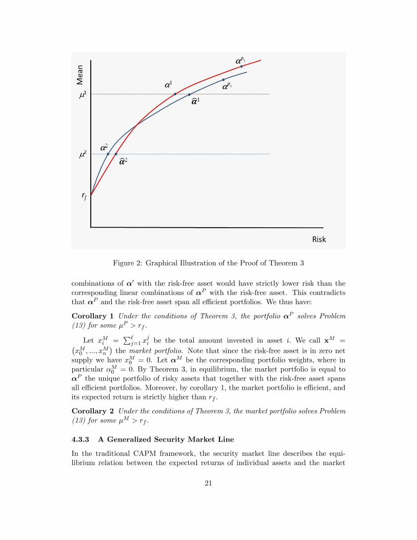
Figure 2: Graphical Illustration of the Proof of Theorem 3

combinations of α′ with the risk-free asset would have strictly lower risk than thecorresponding linear combinations of αP with the risk-free asset. This contradictsthat αP and the risk-free asset span all effi cient portfolios. We thus have:

Corollary 1 Under the conditions of Theorem 3, the portfolio αP solves Problem(13) for some µP > rf .

Let xMi =∑`

j=1 xji be the total amount invested in asset i. We call x

M =(xM0 , ..., xMn

)the market portfolio. Note that since the risk-free asset is in zero net

supply we have xM0 = 0. Let αM be the corresponding portfolio weights, where inparticular αM0 = 0. By Theorem 3, in equilibrium, the market portfolio is equal toαP the unique portfolio of risky assets that together with the risk-free asset spansall effi cient portfolios. Moreover, by corollary 1, the market portfolio is effi cient, andits expected return is strictly higher than rf .

Corollary 2 Under the conditions of Theorem 3, the market portfolio solves Problem(13) for some µM > rf .

4.3.3 A Generalized Security Market Line

In the traditional CAPM framework, the security market line describes the equi-librium relation between the expected returns of individual assets and the market

21

expected return. In particular, the expected return of any asset in excess of therisk-free rate is proportional to the excess market expected return, with the propor-tion being equal to the traditional beta. The following theorem provides suffi cientconditions under which a similar relation holds with respect to our Aumann-Shapleybased systematic risk measure.

Theorem 4 Consider an equilibrium with positive prices and let αM be the marketportfolio. Assume that R (·) is homogeneous of some degree k, smooth, convex, andsatisfies the risk-free property. Then, for each asset i = 1, ..., n,

E (zi) = rf + BRi(E(αM · z

)− rf

), (15)

where

BRi =Ri(αM

)∑nj=1 α

Mj Rj (αM )

=Ri(αM

)kR (αM )

is the scaled Aumann-Shapley measure of systematic risk.

As an illustration, consider

R (·) = θm2 (·) + (1− θ)√m4 (·) (16)

for θ ∈ [0, 1]. This risk measure captures both variance and tail risk, and it satisfies allof the conditions in Theorem 4. Moreover, the utility function V j derived from thisrisk measure is a local expected utility in the sense of Machina (1982), see AppendixII. It is straightforward to verify that

BRi =θCov (zi,α · z) + (1− θ) (m4 (α · z))−

12 Cov

(zi, (α· (z−E (z)))3

)θm2 (α · z) + (1− θ) (m4 (α · z))

12

(17)

=R1 (x)

R (x)BR1i (x) +

R2 (x)

R (x)BR2i (x) ,

where R1 (·) = θm2 (·) and R2 (·) = (1− θ)√m4 (·).

4.3.4 Discussion

Before concluding this section we point out two additional issues. First, while wedescribed suffi cient conditions under which two-fund money separation holds and usethis to argue that the market portfolio is effi cient, these conditions are by no meansnecessary. Weaker conditions that guarantee two-fund money separation may exist.Further, even when two-fund money separation fails, it does not necessarily meanthat market effi ciency is rejected. The literature explores market effi ciency fromboth theoretical (see, for example, Dybvig and Ross (1982)) and empirical (see, forexample, Levy and Roll (2010)) views. Our generalized SML remains valid as longas we have evidence that the market portfolio is mean-risk effi cient.

Second, the SML pricing formula (15) can indeed be applied not only to themarket portfolio, but with respect to any effi cient portfolio. Specifically, suppose

22

that α∗ represents a portfolio that is mean-risk effi cient. Then, it can be easily seenfrom the proof of Theorem (4) that in equilibrium, we have for each asset i,

E (zi) = rf +Ri (α∗)

kR (α∗)(E (α∗ · z)− rf ) .

5 Conclusion

In this paper we develop a general framework to measuring systematic risk, thecontribution of an asset to the risk of a portfolio of assets. Our axiomatic approachspecifies four economically meaningful conditions that pin down a unique measure ofsystematic risk. Our equilibrium approach shows that results attributed to the classicCAPM hold much more broadly. In particular, aspects of the geometry of effi cientportfolios, two fund money separation, and the security market line are derived ina setting where risk can account for a variety of attributes. Both approaches leadto the conclusion that systematic risk should be measured as a scaled version of theAumann-Shapley (1974) diagonal formula.

When risk is confined to measure the variance of a distribution, our systematicrisk measure coincides with beta, the slope from regressing asset returns on portfolioreturns. More generally, systematic risk is not a regression coeffi cient. Rather, itshould be interpreted as the average of the marginal contributions of an asset to therisk of portfolios along a diagonal from the original to the portfolio of interest. Thisinterpretation takes a particularly simple form when the risk measure is homogeneous.In these cases systematic risk is simply the marginal contribution of the asset to therisk of the portfolio of interest, scaled by the weighted average of all such marginalcontributions.

Our axiomatic approach applies to a wide variety of risk measures, requiring ofthem only smoothness and zero risk for zero investment. The equilibrium frameworkimposes additional conditions in the form of homogeneity, convexity, and the risk-freeproperty. Nevertheless, even in the equilibrium framework we are still left with anextensive class of risk measures. Indeed, this class is suffi ciently broad to potentiallyaccount for high distribution moments, rare disasters, downside risk, as well as manyother aspects of risk. Future research may direct at developing weaker conditionsthat further expand the set of applicable risk measures that can be studied in anequilibrium framework.

Finally, our framework is agnostic regarding the choice of a particular risk mea-sure. Indeed, which risk measures better capture the risk preferences of investors isultimately an empirical question. Our framework therefore provides foundations fortesting the appropriateness of risk measures and consequently selecting those thatare supported by the data.

References

[1] Acharya, Viral V., Lasse H. Pedersen, Thomas Philippon, and Mathew Richard-son, 2010. ‘Measuring systemic risk.’Working Paper, New York University.

23

[2] Adrian, Tobias, and Markus K. Brunnermeier, 2011. ‘CoVaR.’ Fed ReserveBank of New York Staff Reports.

[3] Aumann, Robert J., and Roberto Serrano, 2008. ‘An economic index of riskiness.’Journal of Political Economy, 116, 810-836.

[4] Aumann, Robert J., and Lloyd S. Shapley, 1974. ‘Values of non-atomic games.’Princeton University Press.

[5] Artzner, Philippe, Freddy Delbaen, Jean-Marc Eber, and David Heath, 1999.‘Coherent measures of risk.’Mathematical Finance, 9, 203-228.

[6] Bansal, Ravi, and Amir Yaron, 2005. ‘Risks for the long run: A potentialresolution of asset pricing puzzles.’ Journal of Finance, 59, 1481-1509.

[7] Barro, Robert J., 2006. ‘Rare disasters and asset markets in the twentiethcentury.’Quarterly Journal of Economics, 121, 823-866.

[8] Barro, Robert J., 2009. ‘Rare disasters, asset prices, and welfare costs.’AmericanEconomic Review, 99, 243-264.

[9] Billera, Louis J., and David C. Heath, 1982. ‘Allocation of shared costs: A setof axioms yielding a unique procedure.’Mathematics of Operations Research, 7,32-39.

[10] Billera, Louis J., David C. Heath, and Joseph Raanan, 1978. ‘Internal tele-phone billing rates - A novel application of non-atomic game theory.’OperationsResearch, 26, 956-965.

[11] Billera, Louis J., David C. Heath, and Robert E. Verrecchia, 1981. ‘A uniqueprocedure for allocating common costs from a production process.’Journal ofAccounting Research, 19, 185-196.

[12] Campbell, John Y., and John H. Cochrane, 1999. ‘By force of habit: Aconsumption-based explanation of aggregate stock market behavior.’ Journalof Political Economy, 107, 205—251.

[13] Cass, David, and Joseph E. Stiglitz, 1970. ‘The structure of investor preferencesand asset returns, and separability in portfolio allocation: A contribution to thepure theory of mutual funds.’ Journal of Economic Theory, 2, 122-160.

[14] Chen, Hui, Scott Joslin, and Ngoc-Khanh Tran, 2012. ‘Rare disasters and risksharing with heterogeneous beliefs.’Review of Financial Studies, 25, 2189-2224.

[15] Dybvig, Philip, and Fang Liu, 2012. ‘On investor preferences and mutual fundseparation.’Working paper, Washington University in St. Louis.

[16] Dybvig, Philip H., and Stephen A. Ross, 1982. ‘Portfolio effi cient set.’ Econo-metrica, 50, 1525-1546.

24

[17] Epstein, Larry G., and Stanley E. Zin, 1989. ‘Substitution, risk aversion, and thetemporal behavior of consumption and asset returns: A theoretical framework.’Econometrica, 57, 937—969.

[18] Foster, Dean P., and Sergiu Hart, 2009. ‘An operational measure of riskiness.’Journal of Political Economy, 117, 785-814.

[19] Foster, Dean P., and Sergiu Hart, 2013. ‘A wealth-requirement axiomatizationof riskiness.’Theoretical Economics, 8, 591-620.

[20] Gabaix, Xavier, 2008. ‘Variable rare disasters: A tractable theory of ten puzzlesin macro-finance.’American Economic Review, 98, 64-67.

[21] Gabaix, Xavier, 2012. ‘Variable rare disasters: An exactly solved framework forten puzzles in macro-finance.’Quarterly Journal of Economics, 127, 645-700.

[22] Gourio, François, 2012. ‘Disaster risk and business cycles.’American EconomicReview, 102, 2734-2766.

[23] Hadar, Josef, and William R. Russell, 1969. ‘Rules for ordering uncertainprospects.’American Economic Review, 59, 25-34.

[24] Hanoch, Giora, and Haim Levy, 1969. ‘The effi ciency analysis of choices involvingrisk.’Review of Economic Studies, 36, 335-346.

[25] Hart, Sergiu, 2011. ‘Comparing risks by acceptance and rejection.’ Journal ofPolitical Economy, 119, 617-638.

[26] Harvey, Campbell R., and Akhtar Siddique, 2000. ‘Conditional skewness in assetpricing tests.’ Journal of Finance, 55, 1263-1295.

[27] Jean, William H., 1971. ‘The extension of portfolio analysis to three or moreparameters.’ Journal of Financial and Quantitative Analysis, 6, 505-515.

[28] Kadan, Ohad, and Fang Liu, 2013. ‘Performance evaluation with high momentsand disaster risk.’Working paper, Washington University in St. Louis.

[29] Kane, Alex, 1982. ‘Skewness preference and portfolio choice.’Journal of Finan-cial and Quantitative Analysis, 17, 15-25.

[30] Kraus, Alan, and Robert H. Litzenberger, 1976. ‘Skewness preference and thevaluation of risk assets.’ Journal of Finance, 31, 1085-1100.

[31] Levy, Moshe, and Richard Roll, 2010. ‘The market portfolio may bemean/variance effi cient after all.’Review of Financial Studies, 23, 2464-2491.

[32] Lintner, John, 1965a. ‘The valuation of risk assets and the selection of riskyinvestments in stock portfolios and capital budgets.’ Review of Economics andStatistics, 47, 13-37.

25

[33] Lintner, John, 1965b. ‘Security prices, risk, and maximal gains from diversifica-tion.’ Journal of Finance, 20, 587-615.

[34] Luenberger, David G., 1969. ‘Optimization by vector space methods.’ JohnWiley & Sons, Inc.

[35] Machina, Mark J., 1982. ‘“Expected utility”analysis without the independenceaxiom.’Econometrica, 50, 277-323.

[36] Mertens, Jean-François, 1980. ‘Values and derivatives.’Mathematics of Opera-tions Research, 5, 523-552.

[37] Mossin, Jan, 1966. ‘Equilibrium in a capital asset market.’ Econometrica, 34,768—783.

[38] Müller, Sigrid M., and Mark J. Machina, 1987. ‘Moment preferences and poly-nomial utility.’ Economics Letters, 23, 349-353.

[39] Nielsen, Lars T., 1989. ‘Asset market equilibrium with short-selling.’Review ofEconomic Studies, 56, 467-473.

[40] Nielsen, Lars T., 1990. ‘Existence of equilibrium in CAPM.’Journal of EconomicTheory, 52, 223-231.

[41] Nielsen, Lars T., 1992. ‘Positive prices in CAPM.’ Journal of Finance, 47,791-808.

[42] Powers, Michael R., 2007. ‘Using Aumann-Shapley values to allocate insurancerisk: The case of inhomogeneous losses.’North American Actuarial Journal, 11,113-127.

[43] Ross, Stephen A., 1978. ‘Mutual fund separation in financial theory: The sepa-rating distributions.’ Journal of Economic Theory, 17, 254-286.

[44] Rothschild, Michael, and Joseph E. Stiglitz, 1970. ‘Increasing risk I: A definition.’Journal of Economic Theory, 2, 225-243.

[45] Samet, Dov, Yair Tauman, and Israel Zang, 1984. ‘An application of theAumann-Shapley prices for cost allocation in transportation problems.’Mathe-matics of Operations Research, 9, 25-42.

[46] Shapley, Lloyd S., 1953. ‘A value for n-person games.’Annals of MathematicalStudies, 28, 307-317.

[47] Sharpe, William F., 1964. ‘Capital asset prices: A theory of market equilibriumunder conditions of risk.’ Journal of Finance, 19, 425-442.

[48] Tarashev, Nikola A., Claudio E. V. Borio, and Kostas Tsatsaronis, 2010. ‘At-tributing systemic risk to individual institutions.’BIS Working Paper No. 308.

26

[49] Tobin, James, 1958. ‘Liquidity preferences as behavior towards risk.’Review ofEconomic Studies, 25, 65-86.

[50] Wachter, Jessica A., 2013. ‘Can time-varying risk of rare disasters explain ag-gregate stock market volatility?’ Journal of Finance, 68, 987-1035.

Appendix I: Proofs

Proof of Theorem 1: Consider a risk allocation problem (R,x) of order n givensome underlying risky assets z = (z1, ..., zn) . Since R is smooth and satisfies R (0) = 0we can view (R,x) as a cost allocation problem as defined in Billera and Heath (1982,hereafter BH). Let c denote a cost allocation procedure as defined in BH. That is,for each cost allocation problem (R,x) of order n, c (R,x) ∈ Rn, and should beinterpreted as the cost allocated to each of the n goods or services. We can thenconsider a natural mapping between systematic risk measures and cost allocationprocedures as follows. If BR (x) is a systematic risk measure of the risk allocationproblem (R,x) , then

c (R,x) =BR (x)R (x · z)

x, (18)

is a cost allocation procedure for the corresponding cost allocation problem (R,x) .Namely, risk allocation measures can be viewed as scaled versions of cost allocationprocedures for the corresponding problems.

Claim 5 A systematic risk measure BR (x) satisfies Axioms 1-4 if and only if thecorresponding cost allocation procedure c (R,x) satisfies Conditions (2.1)-(2.4) in BH.

It is important to note that we do not argue that Axioms 1-4 and Conditions(2.1)-(2.4) in BH are equivalent individually. Rather, our four axioms as a set areequivalent to their four conditions as a set.

The proof of this claim follows from the following four steps, which apply to anyrisk allocation problem and corresponding cost allocation problem of order n.

Step 1. Axiom 1 is satisfied if and only if Condition (2.1) holds. Indeed,∑n

i=1 αiBRi (x) =

1 is equivalent to∑n

i=1xiR(x)BRi (x)

x = R (x) , which using (18) is equivalent to∑n

i=1 xici (R,x) =R (x) . This is Condition (2.1).

Step 2. Axiom 2 is satisfied if and only if Condition (2.2) holds. Indeed, supposeR (·) = R1 (·) +R2 (·) and

BRi (x) =R1 (x)

R (x)BR1i (x) +

R2 (x)

R (x)BR2i (x) .

ThenBRi (x)R (x)

x=R1 (x)BR1i (x)

x+R2 (x)BR2i (x)

x.

27

That is,c (R,x) = c

(R1,x

)+ c

(R2,x

),

which is Condition (2.2). The other direction is similar (recalling that R (x) 6= 0).

Step 3. Condition (2.3) implies Axiom 3. Axioms 1 and 3 jointly imply Condition(2.3).

Assume first that Condition (2.3) in BH holds. Suppose that z = (z1, ..., zn) areR-perfectly correlated. Then, for any η ∈ Rn, R (η · z) = g (η · q) for some functiong (·) and a non-zero q ∈ Rn. Condition (2.3) implies that ci (R,x) = c (g,x · q) qi fori = 1, ..., n. It follows that for all i, j = 1, ..., n

qjci (R,x) = qicj (R,x) .

Applying (18) we obtain that Axiom 3 is satisfied.Assume now that both Axioms 1 and 3 are satisfied and assume that for all

η ∈ Rn,R (η · z) = g (η · q) (19)

for some function g (·) and a non-zero vector q ∈ Rn. Then, (z1, ..., zn) are R-perfectlycorrelated.

By Axiom 3 for all i, j = 1, ..., n

qjBRi (x) = qiBRj (x) . (20)

By Axiom 1 we know that∑k

i=1 αiBRi (x) = 1. Plugging (20) we have

qj =n∑i=1

αiqiBRj (x) = (α · q)BRj (x) for j = 1, ..., n.

By (18), and recalling that R (x) 6= 0

qj = (α · q)cj (R,x) x

R (x)= (x · q)

cj (R,x)

R (x)for j = 1, ..., n. (21)

If x · q = 0 this implies that qj = 0 for all j, contradicting that q is a non-zerovector. Hence, x · q is not zero. We then have

cj (R,x) =qjR (x)

(x · q)for all j = 1, .., n. (22)

Consider an asset with return w = x·zx·q . Namely, investing x ·q dollars in this asset

yields the same return as of the portfolio x. Then,

R ((x · q) w) = R (x · z) = g (x · q) .

Consider now the risk allocation problem of order 1 with the single asset w heldat the amount x ·q. By Axiom 1 the systematic risk measure of this asset must satisfy

BR (x · q) = 1,

28

or equivalently using (18),

c (g,x · q) =R ((x · q) w)

x · q =g (x · q)

x · q .

Plugging back into (22) and using that R (x) = g (x · q) we have

cj (R,x) = c (g,x · q) qj ,

which is exactly what Condition (2.3) in BH requires.

Step 4. Axiom 4 is satisfied if and only if Condition (2.4) holds. This follows directlyfrom (18) and the definition of R-positive correlation.

Having established this claim we can now rely on the main theorem in BH toconclude that the unique cost allocation procedure associated with any risk allocationproblem (R,x) (and its corresponding cost allocation problem) of order n satisfyingAxioms 1-4 is given by.

ci (R,x) =

∫ 1

0Ri (tx) dt.

Applying (18) we obtain that the unique systematic risk measure satisfying Axioms1-4 is given by (8).

Finally, to see that (8) and (9) are equivalent when R is homogenous of degree k,note first that in this case∫ 1

0Ri (tx1, ..., txn) dt = Ri (x1, ..., xn)

∫ 1

0tk−1dt

=Ri (x1, ..., xn)

k,

where the first equality follows since Ri is homogeneous of degree k − 1. It followsthat

BRi (x) =x∫ 1

0 Ri (tx1, ..., txn) dt

R (x1, ..., xn)

=xRi (x1, ..., xn)

kR (x1, ..., xn)

=xRi (xα1, ..., xαn)

kR (xα1, ..., xαn)

=Ri (α1, ..., αn)

kR (α1, ..., αn)

=Ri (α1, ..., αn)∑n

j=1 αjRj (α1, ..., αn),

where the the penultimate equality follows from the homogeneity of degrees k andk−1 of R and Ri respectively, and the last equality follows from Euler’s homogeneousfunction theorem. This completes the proof of Theorem 1.

29

Proof of Proposition 1: The partial derivatives of R (·) with respect to the portfolioweights are given by ∀i,

Ri (α1, ..., αn) = kE

(zi − E (zi))

n∑j=1

αj (zj − E (zj))

k−1

= kE[(zi − E (zi)) (α · z−α·E (z))k−1

]= kCov

(zi, (α · z−α·E (z))k−1

).

Thus, using (10), the systematic risk of asset i becomes

BRi =Cov

(zi, (α · z−α·E (z))k−1

)E[(α · z−α·E (z))k

] .

Proof of Proposition 2: When R (·) = RAS (·) , R (α) is implicitly determined by

E

[exp

(− α · zR (α)

)]= 1.

By the implicit function theorem,

Ri (α) =E[exp

(− α·zR(α)

)zi

R(α)

]E[exp

(− α·zR(α)

)α·z

(R(α))2

]= R (α)

E[exp

(− α·zR(α)

)zi

]E[exp

(− α·zR(α)

)α · z

] .Since the AS measure is homogeneous of degree 1, (10) becomes

BRi =E[exp

(− α·zR(α)

)zi

]E[exp

(− α·zR(α)

)α · z

] .The proof for the FH measure is similar.

Proof of Proposition 3: What we need to show is that for any random returns z1

and z2, and any 0 ≤ λ ≤ 1,

wk (λz1 + (1− λ) z2) ≤ λwk (z1) + (1− λ)wk (z2) . (23)

Letting z1 = z1 − E (z1) and z2 = z2 − E (z2) , (23) can be rewritten as(E[(λz1 + (1− λ) z2)k

]) 1k ≤ λ

(E[zk1

]) 1k

+ (1− λ)(

E[zk2

]) 1k. (24)

30

From the binomial formula we know that for any two numbers p and q,

(p+ q)k =k∑i=0

(k

i

)pk−iqi.

Applying this to the LHS of (24) implies that we need to show(k∑i=0

(k

i

)λk−i (1− λ)i E

(zk−i1 zi2

)) 1k

≤ λ(

E[zk1

]) 1k

+ (1− λ)(

E[zk2

]) 1k.

Since k is even, replacing each z1 and z2 with |z1| and |z2| will not affect the RHS,but it might increase the LHS. So, it is suffi cient to show that(

k∑i=0

(k

i

)λk−i (1− λ)i E

(∣∣∣zk−i1 zi2

∣∣∣))1k

≤ λ(

E[|z1|k

]) 1k

+ (1− λ)(

E[|z2|k

]) 1k.

Since both sides are positive we can raise both sides to the kth power, maintainingthe inequality. Thus, it would be suffi cient to show

k∑i=0

(k

i

)λk−i (1− λ)i E

(∣∣∣zk−i1 zi2

∣∣∣) ≤ (λ(E[|z1|k

]) 1k

+ (1− λ)(

E[|z2|k

]) 1k

)k.

Applying the binomial formula to the RHS implies that it would be suffi cient to show

k∑i=0

(k

i

)λk−i (1− λ)i E

(∣∣∣zk−i1 si∣∣∣) ≤ k∑

i=0

(k

i

)λk−i (1− λ)i

(E[|z1|k

]) k−ik(

E[|z2|k

]) ik.

To establish this inequality we will show that it actually holds term by term.That is, it is suffi cient to show that for each i = 0, ..., k,

E(∣∣∣zk−i1 zi2

∣∣∣) ≤ (E[|z1|k

]) k−ik(

E[|z2|k

]) ik.

To see this, note that it is equivalent to show that

E(∣∣∣zk−i1 si

∣∣∣) ≤ (E

[∣∣∣zk−i1

∣∣∣ kk−i]) k−i

k(

E

[∣∣zi2∣∣ ki ]) ik

.

Now, denote Z1 = zk−i1 , Z2 = zi2, p = kk−i and q = k

i . Note that1p + 1

q = 1. Then,what we need to show is

E (|Z1Z2|) ≤ E (|Z1|p)1p E (|Z2|q)

1q .

But, this is immediate from Holder’s inequality, and we are done.

Proof of Proposition 4: In the definition of Expected Short-fall we assumed theexistence of a cumulative distribution function F (·) applied to realizations of random

31

variables. For the sake of this proof it will be more useful to work directly with theprobability space Ω and with the underlying probability measure P (·) .We first provethat ESα(z) is subadditive. That is, for any two random returns z1 and z2,

ESα(z1 + z2) ≤ ESα(z1) + ESα(z2). (25)

By definition, for any random return z, ESα (z) can be expressed as

ESα (z) = − 1

α

∫ω:z≤−VaRα(z)

zdP (ω) .

Define z3 = z1 + z2. Let Ωi = ω ∈ Ω : zi ≤ −VaRα (zi) for i = 1, 2, 3. Then, (25) isequivalent to ∫

Ω3

z3dP (ω) ≥∫

Ω1

z1dP (ω) +

∫Ω2

z2dP (ω) ,

which can be rewritten as∫Ω3

z1dP (ω) +

∫Ω3

z2dP (ω) ≥∫

Ω1

z1dP (ω) +

∫Ω2

z2dP (ω) .

This is true if we have ∫Ω3

z1dP (ω) ≥∫

Ω1

z1dP (ω) , (26)

and ∫Ω3

z2dP (ω) ≥∫

Ω2

z2dP (ω) . (27)

For brevity, we will only prove (26) below. The proof of (27) is parallel.To prove (26), define Ω4 = ω ∈ Ω : z1 ≤ −VaRα (z1) , z3 ≤ −VaRα (z3) , Ω5 =

ω ∈ Ω : z1 ≤ −VaRα (z1) , z3 > −VaRα (z3) and Ω6 = ω ∈ Ω : z1 > −VaRα (z1) , z3 ≤ −VaRα (z3) .Since Ω4 ∩ Ω5 = ∅, Ω4 ∪ Ω5 = Ω1, and Ω4 ∩ Ω6 = ∅, Ω4 ∪ Ω6 = Ω3, we have that∫

Ω1

dP (ω) =

∫Ω4

dP (ω) +

∫Ω5

dP (ω) ,

and ∫Ω3

dP (ω) =

∫Ω4

dP (ω) +

∫Ω6

dP (ω) .

By the definition of VaR, we know∫Ω1

dP (ω) =

∫Ω3

dP (ω) = α.

Thus, we obtain ∫Ω5

dP (ω) =

∫Ω6

dP (ω) . (28)

Similarly, we know ∫Ω1

z1dP (ω) =

∫Ω4

z1dP (ω) +

∫Ω5

z1dP (ω) ,

32

and ∫Ω3

z1dP (ω) =

∫Ω4

z1dP (ω) +

∫Ω6

z1dP (ω) .

Hence, ∫Ω1

z1dP (ω)−∫

Ω3

z1dP (ω)

=

∫Ω5

z1dP (ω)−∫

Ω6

z1dP (ω)

≤∫

Ω5

[−VaRα (z1)] dP (ω)−∫

Ω6

[−VaRα (z1)] dP (ω)

= −VaRα (z1)

[∫Ω5

dP (ω)−∫

Ω6

dP (ω)

],

where the inequality follows from z1 ≤ −VaRα (z1) when ω ∈ Ω5 and z1 > −VaRα (z1)when ω ∈ Ω6. By (28), we have∫

Ω5

dP (ω)−∫

Ω6

dP (ω) = 0,

which implies ∫Ω1

z1dP (ω)−∫

Ω3

z1dP (ω) ≤ 0.

Therefore, (26) is obtained, and hence ESα(z) is subadditive.Then, convexity follows immediately from homogeneity and subadditivity, since

for any λ ∈ [0, 1] ,

ESα(λz1 + (1− λ) z2) ≤ ESα(λz1) + ESα((1− λ) z2)

= λESα(z1) + (1− λ) ESα(z2).

Proof of Lemma 2: Our setting is a special case of the setting in Nielsen (1989).To show the existence of equilibrium Nielsen requires that preferences satisfy thefollowing three conditions: (i) each investor’s choice set is closed and convex, andcontains her initial endowment; (ii) The set of

ζ ∈ Rn+1 : U j (ζ) ≥ U j

(ζ′)is closed

for all ζ′ ∈ Rn+1 and for all j = 1, ..., `; (iii) If ζ, ζ′ ∈ Rn+1 and U j(ζ′)> U j (ζ) ,

then U j(tζ′ + (1− t)ζ) > U j(ζ) for all t in (0, 1).Condition (i) is satisfied in our setting since the choice set of each investor is

Rn+1, which is closed and convex, and contains ej for all j. Condition (ii) holdssince V is assumed continuous and R is assumed smooth, and so their compositionis continuous. Condition (iii) follows since V (·) is quasi-concave, strictly increasingin its first argument and strictly decreasing in its second argument, and R (·) is aconvex risk measure.

Given these properties of the preferences, Nielsen (1989) establishes two conditionsas suffi cient for the existence of a quasi-equilibrium: (i) positive semi-independence

33

of directions of improvement, and (ii) non-satiation at Pareto attainable portfolios.Condition (i) follows in our setting as in Nielsen (1990, Proposition 1) since in our set-ting all investors agree on all parameters of the problem (in particular on the expectedreturns), and due to the non-redundancy of risky assets assumption. To see why con-dition (ii) holds in our setting note that we assume the existence of a risk-free assetpaying a non-zero payoffwith probability 1. Since R (·) satisfies the risk-free property,we have that R (z1 + z2) ≤ R (z1) whenever z2 is R-risk-free with P (z2 > 0) = 1.Thus, adding a positive risk-free asset can only (weakly) reduce risk. It follows thatwe can always add this positive risk-free asset to any bundle ζ, strictly increasing theexpected return while weakly decreasing risk. This implies that in our model thereis no satiation globally. Thus, a quasi-equilibrium exists in our setting. Moreover,any quasi-equilibrium is, in fact, an equilibrium in our setting. This follows from theconditions in Nielsen (1989 p. 469). Indeed, in our setting each investor’s choice setis convex and unbounded, and the set

ζ ∈ Rn+1 : U j (ζ) > U j

(ζ′)is open for all

j and ζ′ ∈ Rn+1.

Proof of Theorem 2: Suppose that the equilibrium bundle of investor j is ζj . Letxj =

∑ni=0 x

ji = p · ζj be the total dollar amount of investment of investor j. Then,

U j(ζj)

= V j

(E

(n∑i=0

ζji yi

), R

(n∑i=0

ζji yi

))(29)

= V j

(xjE

(n∑i=0

ζjixjyi

),(xj)kR

(n∑i=0

ζjixjyi

))

= V j

(xjE

(n∑i=0

ζjipixj

yipi

),(xj)kR

(n∑i=0

ζjipixj

yipi

))

= V j

(xjE

(n∑i=0

xjixjzi

),(xj)kR

(n∑i=0

xjixjzi

))

= V j

(xjE

(n∑i=0

αji zi

),(xj)kR

(n∑i=0

αji zi

))= V j

(xjE

(αj ·z

),(xj)kR(αj ·z

)),

where k is the degree of homogeneity of R (·) . From the definition of equilibrium,each investor chooses ζj to maximize U j

(ζj)subject to xj ≤ p · ej , where in equi-

librium xj = p · ej is given. From (29) and since V j is strictly increasing in the firstargument and strictly decreasing in the second argument, we have that for any posi-tive xj , U j

(ζj)is strictly increasing in E

(αj ·z

)and strictly decreasing in R

(αj ·z

).

Therefore, in equilibrium, αj must minimize R (α · z) for a given level of expectedreturn E

(αj ·z

), and thus solve Problem (13). The solution is unique since we as-

sumed that R (·) is a convex risk measure, and so R (α · z) is convex as a function ofα.

34

Proof of Theorem 4: Since R (·) is smooth and by Lemma 2 the solution toProblem (13) for some µj = µ is determined by the first order conditions. To solvethis program, form the Lagrangian

L (α) = R (α)− λ(

n∑i=1

αiE (zi) +

(1−

n∑i=1

αi

)rf − µ

),

where λ is a Lagrange multiplier. Equivalently,

L (α) = R

(1−

n∑i=1

αi, α1, ..., αn

)− λ

(n∑i=1

αiE (zi) +

(1−

n∑i=1

αi

)rf − µ

)

The first order condition states that ∀i = 1, ..., n,

−R0 (α∗) +Ri (α∗)− λ (E (zi)− rf ) = 0, (30)

where α∗ represents the optimal portfolio. By the risk-free property, R0 (α∗) = 0.Hence,

Ri (α∗)− λ (E (zi)− rf ) = 0. (31)

Multiplying by α∗i , we obtain

α∗iRi (α∗)− λα∗i (E (zi)− rf ) = 0.

Summing up over i = 1, ..., n yields

n∑i=1

α∗iRi (α∗)− λn∑i=1

α∗i (E (zi)− rf ) = 0.

Noting again that R0 (α∗) = 0, this is equivalent to

n∑i=0

α∗iRi (α∗)− λn∑i=1

α∗i (E (zi)− rf ) = 0.

By Euler’s homogeneous function theorem, we can rewrite this as

kR (α∗)− λn∑i=1

α∗i (E (zi)− rf ) = 0.

Adding and subtracting rf inside the summation yields

kR (α∗)− λ(

n∑i=1

α∗iE (zi) + rf

(1−

n∑i=1

α∗i

)− rf

)= 0,

which by the optimization constraint is equivalent to

kR (α∗)− λ (µ− rf ) = 0.

35

Hence,

λ =kR (α∗)

µ− rf. (32)

Plugging (32) into (31) gives

Ri (α∗)− kR (α∗)

µ− rf(E (zi)− rf ) = 0,

which can be rewritten as

E (zi) = rf +Ri (α∗)

kR (α∗)(µ− rf ) . (33)

This result applies to any effi cient portfolio α∗. By Corollary 2, the market port-folio is effi cient, and hence

E (zi) = rf +Ri(αM

)kR (αM )

(µM − rf

).

as claimed.

Appendix II: Mean-Risk Preferences and Expected Util-ity

Background

One would wonder how the mean-risk preferences considered in Section 4 are relatedto the commonly assumed von Neumann-Morgenstern utility. It is widely knownthat a von Neumann-Morgenstern investor with a quadratic utility function onlycares about the mean and the variance of his investments in the sense that he prefersa high expected wealth and a low variance. In this sense, the mean-risk preferenceis consistent with the von Neumann-Morgenstern utility when variance is used asthe risk measure. Alternatively, when returns are distributed according to a two-parameter elliptical distribution (normal being a special case), mean-variance prefer-ences can also be supported by expected utility. These instances, however, are quiterestrictive. First, the quadratic utility is not very intuitive since it implies increas-ing absolute risk aversion. Second, elliptical distributions, being determined by thefirst two moments only, limit our ability to describe the dependence of risk on highdistribution moments. Thus, in general, mean-variance preferences or not consistentwith expect-utility. The approach taken in this paper is much more general, allowingfor a variety of risk measures. Whether a particular risk measure is consistent withexpected utility depends on the actual choice of the risk measure. For example, riskmeasures that are simple linear combinations of raw moments up to the kth degree canbe represented by a kth degree polynomial (Müller and Machina (1987)), generalizingthe mean-variance result.

While in general the preferences defined in (12) cannot be supported by expectedutility, they are often consistent with expected utility locally. The idea is based on

36

Machina’s (1982) “Local Utility Function.”To facilitate this approach we first restrictattention to risk measures that depend on the distribution of the random variablesonly. Thus, we consider risk measures that are functions from the distribution ofrealizations to the reals rather than functions from the random variables themselves.Practically, this does not present a binding restriction since all the examples in thispaper and all standard risk measures only rely on the distribution of realizationsanyway. In this case the preferences in (12) can be written as

U (ζ) = V(E(Fζ·y

), R(Fζ·y

)),

where Fζ·y is the cumulative distribution of the random variable ζ · y. When therandom variable in question is clear, we will omit it from the notation and write theutility as U (F ) = V (E (F ) , R (F )) .

According to Machina (1982), if the realizations of all random variables are con-tained in some bounded and closed interval I and U (F ) is Fréchet differentiablewith respect to the L1 norm,9 then for any two distributions F1, F2 on I there existsu (·;F1) differentiable almost everywhere on I such that

U (F2)− U (F1) =

∫Iu (y;F1) dF2 (y)−

∫Iu (y;F1) dF1 (y) + o (‖F2 − F1‖) , (34)

where ‖·‖ denotes the L1 norm. That is, starting from a wealth distribution F1, if aninvestor moves to another “close”distribution F2, then he compares the utility fromthese two distributions as if he is maximizing his expected utility with a local utilityfunction u (·;F1) .

The key to applying Machina’s result is to find suffi cient conditions on the riskmeasure which guarantee that U (F ) is Fréchet differentiable. This can be done inmany ways. Next we provide one simple but effective approach which is suffi cient tovalidate many popular risk measures as consistent with local expected utility.

Risk Measures as Functions of Moments

Let µFk =∫yjdF (y) be the kth raw moment given distribution F, and mF

k =∫ (y − µF1

)kdF (y) be the kth central moment given distribution F. Consider risk

measures which are a function of a finite number of (raw or central) moments. We

denote such risk measures byR(µFj1 , ..., µ

Fjl,mF

k1, ...,mF

kn

). We assume that R is dif-

ferentiable in all arguments. The utility function in (12) then takes the form

U (F ) = V(µF1 , R

(µFj1 , ..., µ

Fjl,mF

k1 , ...,mFkn

)), (35)

where V is differentiable in both mean and risk. This class of utility functions isquite general and it allows the risk measure to depend on a large number of highdistribution moments. We then have the following proposition.

9Fréchet differentiability is an infinite dimensional version of differentiability. The idea here isthat U (F ) changes smoothly with F, where changes in F are topologized using the L1 norm. SeeLuenberger (1969 p. 171).

37

Proposition 5 If U (F ) takes the form (35) then for any two distributions F1, F2 onI there exists u (·;F1) differentiable almost everywhere on I such that (34) holds.

Proof of Proposition 5: We need to show that U (F ) is Fréchet differentiable. Bythe chain rule for Fréchet differentiability (Luenberger (1969, p. 176), we know thatif both µFk and m

Fk are Fréchet differentiable for any k, then so is U (·) . The Fréchet

differentiability of µFk is obvious, since

µF2k − µF1k =

∫IykdF2 (y)−

∫IykdF1 (y) = −k

∫I

(F2 (y)− F1 (y)) yk−1dy.

Now we show that mFk is Fréchet differentiable. We have

mFk =

∫ (y − µF1

)kdF (y)

=

∫ k∑i=0

k!

i! (k − i)!yi(µF1)k−i

dF (y)

=k∑i=0

k!

i! (k − i)!(µF1)k−i ∫

yidF (y)

=

k∑i=0

k!

i! (k − i)!(µF1)k−i

µFi ,

which is a differentiable function of the µFi ’s. By the chain rule, it follows immediatelythat mF

k is also Fréchet differentiable. This completes the proof.

Appendix III: Suffi cient Conditions for Positive Prices

In this appendix we provide a suffi cient condition for the positivity of equilibriumprices. Let ζ ∈ Rn+1 be a bundle. Denote the gradient of investor j’s utility func-tion at ζ by ∇Uj (ζ) = (U j0 (ζ) , ..., U jn (ζ)), where a subscript designates a partial

derivative in the direction of the ith asset. Also, let γj (ζ) = −V j2 (E(ζ·y),R(ζ·y))

V j1 (E(ζ·y),R(ζ·y))> 0

be the marginal rate of substitution of the expected payoff of the bundle for therisk of the bundle. This is the slope of investor j′s indifference curve in expectedpayoff-risk space. For brevity we often omit the arguments of this expression and use

γj (ζ) = −V j2V j1.

Proposition 6 Assume that for each asset i there is some investor j such thatE(yi) > γj (ζ)Ri (ζ · y) for all ζ. Then, prices of all assets are positive in all equi-libria.

38

Proof: As Nielsen (1992) indicates, at an equilibrium, all investors’gradients pointin the direction of the price vector. So the price of asset i must be positive in anyequilibrium if there is some investor j such that U ji (ζ) > 0 for all ζ. Recall that

U j (ζ) = V j (E (ζ · y) , R (ζ · y)) .

Thus,

U ji (ζ) = V j1 E(yi) + V j

2 Ri (ζ · y)

= V j1 [E(yi)− γj (ζ)Ri (ζ · y)],

where Ri (ζ · y) denotes the partial derivative of R (ζ · y) with respect to ζi.Since V j

1 > 0, U ji (ζ) > 0 corresponds to

E(yi)− γj (ζ)Ri (ζ · y) > 0

as required.Note that γj (·) can serve as a measure of risk aversion for investor j. We can thus

interpret this proposition as follows. If each asset’s expected return is suffi ciently highrelative to some investor’s risk aversion and the marginal contribution of the asset tototal risk, then this asset will always be desirable by some investor, and so, its pricewill be positive in any equilibrium.

39