Embed Size (px)
Citation preview
University of Southern Queensland
Faculty of Health, Engineering & Sciences
Systematic Procedure To Determine Line Current
Differential Relay Settings With Back up Distance for a
500 kV ac Three Phase Line
A dissertation submitted by
Timothy Pasanduka
in fulfilment of the requirements of
ENG4112 Research Project
towards the degree of
Bachelor of Engineering in Power
Submitted: October, 2013
Abstract
A 500 kV overhead line needs adequate protection for power to be transmitted safely
and efficiently. Current differential protection is a type of protection that is used on a
500 kV line. In a three phase network, six matched current transformers are used in
line differential protection. Three current transformers are placed at each end of the
line with one in each phase. The two current transformers at each end of the line on
the same phase are connected in a way to measure the differential current flowing in
their secondary windings.
Distance protection is another form of protection used on a 500 kV line. In a three
phase network, three current transformers and three voltage transformers are employed
at each end of the protected line. This form of protection looks at the impedance of
the line and registers a fault whenever the impedance seen by the relay becomes less
that a set value.
Both current differential and distance protection can be employed at the same time
on the same line. This project looks at a systematic way to determine line current
differential relay settings with distance protection as the back up protection on a 500
kV line.
A simulation of faults to determine system behaviour under the fault condition is carried
out on both modes of protection. In the case of the current differential, in zone and
out of zone faults are simulated using Sim Power Systems.
University of Southern Queensland
Faculty of Health, Engineering and Sciences
ENG4111/2 Research Project
Limitations of Use
The Council of the University of Southern Queensland, its Faculty of Health, Engineer-
ing and Sciences and the staff of the University of Southern Queensland, do not accept
any responsibility for the truth, accuracy or completeness of material contained within
or associated with this dissertation.
Persons using all or any part of this material do so at their own risk, and not at the
risk of the Council of the University of Southern Queensland, its Faculty of Health,
Engineering and Sciences or the staff of the University of Southern Queensland.
This dissertation reports an educational exercise and has no purpose or validity beyond
this exercise. The sole purpose of the course pair entitled “Research Project” is to
contribute to the overall education within the student’s chosen degree program. This
document, the associated hardware, software, drawings, and other material set out in
the associated appendices should not be used for any other purpose: if they are so used,
it is entirely at the risk of the user.
Prof F Bullen
Dean
Faculty of Health, Engineering and Sciences

Certification of Dissertation
I certify that the ideas, designs and experimental work, results, analyses and conclusions
set out in this dissertation are entirely my own effort, except where otherwise indicated
and acknowledged.
I further certify that the work is original and has not been previously submitted for
assessment in any other course or institution, except where specifically stated.
Timothy Pasanduka
0050110872
Signature
Date

Acknowledgments
My thanks go to Dr Tony Ahfock of USQ (University of Southern Queensland) for his
help firstly in putting my ideas together in formulating this project and then monitoring
my progress as the project evolved. Many thanks to my wife Felicity and daughters
Elizabeth, Elaine and Eunice for their unwavering support during the course of this
project. These four girls endured various late late night disturbances as I worked
through the project.
Timothy Pasanduka
University of Southern Queensland
October 2013
Contents
Abstract i
Acknowledgments iv
List of Figures xi
List of Tables xvii
Chapter 1 Introduction 1
1.1 Project Background Information . . . . . . . . . . . . . . . . . . . . . . 2
1.2 Aims and Objectives of this Project . . . . . . . . . . . . . . . . . . . . 2
1.3 Outline of the dissertation . . . . . . . . . . . . . . . . . . . . . . . . . . 3
Chapter 2 Line Current Differential Protection 4
2.1 Chapter Overview . . . . . . . . . . . . . . . . . . . . . . . . . . . . . . 4
2.2 Principle of Line Current Differential Protection . . . . . . . . . . . . . 5
2.3 Matched Current Transformers . . . . . . . . . . . . . . . . . . . . . . . 6
2.4 Pilot Wire Protection . . . . . . . . . . . . . . . . . . . . . . . . . . . . 7
2.4.1 Solkor R . . . . . . . . . . . . . . . . . . . . . . . . . . . . . . . . 8
CONTENTS vi
2.4.2 Solkor RF . . . . . . . . . . . . . . . . . . . . . . . . . . . . . . . 9
2.5 Summation Transformer for Pilot Wire Protection . . . . . . . . . . . . 10
2.6 Line differential Protection Characteristic . . . . . . . . . . . . . . . . . 13
2.6.1 Copper Wire Communications Links . . . . . . . . . . . . . . . . 14
2.7 A Heavily Loaded Line using Current Differential Protection . . . . . . 14
2.8 Current Differential Protection in Teed Lines . . . . . . . . . . . . . . . 16
2.9 Chapter Summary . . . . . . . . . . . . . . . . . . . . . . . . . . . . . . 19
Chapter 3 Distance Protection 20
3.1 Chapter Overview . . . . . . . . . . . . . . . . . . . . . . . . . . . . . . 20
3.2 What is Distance Protection . . . . . . . . . . . . . . . . . . . . . . . . . 20
3.2.1 Relay Performance . . . . . . . . . . . . . . . . . . . . . . . . . . 21
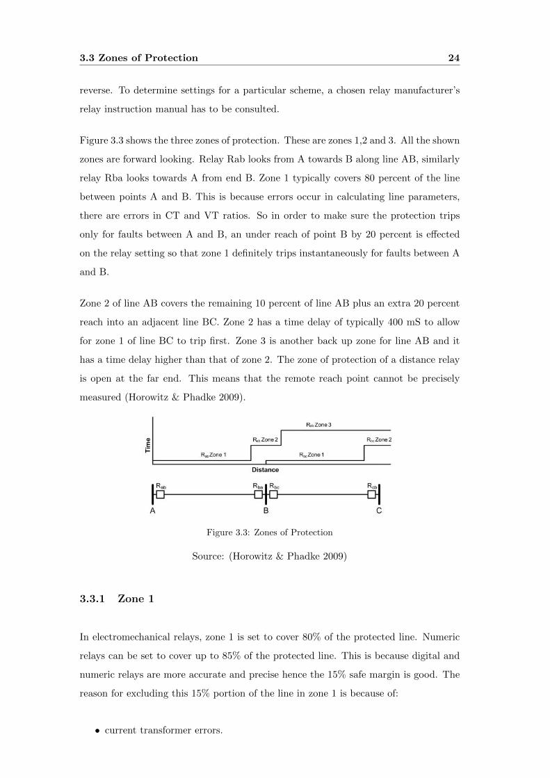
3.3 Zones of Protection . . . . . . . . . . . . . . . . . . . . . . . . . . . . . . 23
3.3.1 Zone 1 . . . . . . . . . . . . . . . . . . . . . . . . . . . . . . . . . 24
3.3.2 Zone 1 Extension . . . . . . . . . . . . . . . . . . . . . . . . . . . 25
3.3.3 Zone 2 . . . . . . . . . . . . . . . . . . . . . . . . . . . . . . . . . 26
3.3.4 Zone 3 . . . . . . . . . . . . . . . . . . . . . . . . . . . . . . . . . 26
3.4 Characteristics . . . . . . . . . . . . . . . . . . . . . . . . . . . . . . . . 27
3.4.1 Mho Characteristic . . . . . . . . . . . . . . . . . . . . . . . . . . 28
3.4.2 Quadrilateral Characteristic . . . . . . . . . . . . . . . . . . . . . 28
3.5 Distance Protection in Parallel Lines . . . . . . . . . . . . . . . . . . . . 29
3.6 Teed Feeders . . . . . . . . . . . . . . . . . . . . . . . . . . . . . . . . . 29
CONTENTS vii
3.7 Distance Protection in a Heavily Loaded Line . . . . . . . . . . . . . . . 29
3.8 Power Swing . . . . . . . . . . . . . . . . . . . . . . . . . . . . . . . . . 33
3.9 Distance Protection Schemes . . . . . . . . . . . . . . . . . . . . . . . . 36
3.9.1 Direct Under-Reach Transfer Scheme . . . . . . . . . . . . . . . . 36
3.9.2 Permissive Under-Reach . . . . . . . . . . . . . . . . . . . . . . . 36
3.9.3 Permissive Over-Reach Transfer Scheme . . . . . . . . . . . . . . 38
3.10 Chapter Summary . . . . . . . . . . . . . . . . . . . . . . . . . . . . . . 39
Chapter 4 Overhead Line Parameters 40
4.1 Chapter Overview . . . . . . . . . . . . . . . . . . . . . . . . . . . . . . 40
4.2 Line models . . . . . . . . . . . . . . . . . . . . . . . . . . . . . . . . . . 40
4.2.1 Short Line . . . . . . . . . . . . . . . . . . . . . . . . . . . . . . . 41
4.2.2 Medium Length Line . . . . . . . . . . . . . . . . . . . . . . . . . 42
4.2.3 Long Line . . . . . . . . . . . . . . . . . . . . . . . . . . . . . . . 43
4.3 Determining Line Parameters . . . . . . . . . . . . . . . . . . . . . . . . 47
4.3.1 Calculation of Line Capacitance . . . . . . . . . . . . . . . . . . 47
4.3.2 Calculation of Line Inductance . . . . . . . . . . . . . . . . . . . 48
4.3.3 Obtaining Line Parameters by Measurements . . . . . . . . . . . 51
4.3.4 Measuring Capacitance using Doble M4100 . . . . . . . . . . . . 52
4.3.5 Line Impedance using Omicron CP CU1 . . . . . . . . . . . . . . 55
4.4 Mutual Coupling and Zero sequence Impedance Measurements . . . . . 58
4.4.1 Line Resistance . . . . . . . . . . . . . . . . . . . . . . . . . . . . 62
CONTENTS viii
4.4.2 Line Parameters Using ASPEN software . . . . . . . . . . . . . . 63
4.5 Chapter Summary . . . . . . . . . . . . . . . . . . . . . . . . . . . . . . 65
Chapter 5 Effect of Line capacitance on Protection Settings 66
5.1 Chapter Overview . . . . . . . . . . . . . . . . . . . . . . . . . . . . . . 66
5.2 Line Capacitance and Pilot wire Protection Protection . . . . . . . . . . 66
5.3 Line Capacitance and Current Differential Protection . . . . . . . . . . . 67
5.4 Line Capacitance and Distance Protection . . . . . . . . . . . . . . . . . 73
5.5 Chapter Summary . . . . . . . . . . . . . . . . . . . . . . . . . . . . . . 79
Chapter 6 Protection Relay 80
6.1 Chapter Overview . . . . . . . . . . . . . . . . . . . . . . . . . . . . . . 80
6.2 SEL 311L . . . . . . . . . . . . . . . . . . . . . . . . . . . . . . . . . . . 80
6.2.1 Current Differential Protection . . . . . . . . . . . . . . . . . . . 81
6.2.2 Distance Protection . . . . . . . . . . . . . . . . . . . . . . . . . 83
6.3 Siemens 7SD5 . . . . . . . . . . . . . . . . . . . . . . . . . . . . . . . . . 86
6.3.1 Further influences . . . . . . . . . . . . . . . . . . . . . . . . . . 88
6.4 GE L90 . . . . . . . . . . . . . . . . . . . . . . . . . . . . . . . . . . . . 89
6.5 Chapter Summary . . . . . . . . . . . . . . . . . . . . . . . . . . . . . . 103
Chapter 7 Systematic Procedure To Determine Relay Settings 104
7.1 Chapter Overview . . . . . . . . . . . . . . . . . . . . . . . . . . . . . . 104
7.2 ASPEN Software for Relay Database . . . . . . . . . . . . . . . . . . . . 104
CONTENTS ix
7.3 Current Differential Protection . . . . . . . . . . . . . . . . . . . . . . . 106
7.3.1 SEL 311L Relay . . . . . . . . . . . . . . . . . . . . . . . . . . . 106
7.3.2 Siemens 7SD5 Relay . . . . . . . . . . . . . . . . . . . . . . . . . 108
7.3.3 GE L90 Current Differential Settings . . . . . . . . . . . . . . . . 112
7.4 Distance Protection . . . . . . . . . . . . . . . . . . . . . . . . . . . . . 114
7.4.1 Siemens 7SD5 . . . . . . . . . . . . . . . . . . . . . . . . . . . . . 114
7.4.2 Over Current and Earth Fault . . . . . . . . . . . . . . . . . . . 116
7.5 Chapter Summary . . . . . . . . . . . . . . . . . . . . . . . . . . . . . . 118
Chapter 8 500 kV Circuit Breaker 119
8.1 Chapter Overview . . . . . . . . . . . . . . . . . . . . . . . . . . . . . . 119
8.2 Circuit Breaker Timing . . . . . . . . . . . . . . . . . . . . . . . . . . . 119
8.3 CB Timing graphs . . . . . . . . . . . . . . . . . . . . . . . . . . . . . . 123
8.4 CB Failure . . . . . . . . . . . . . . . . . . . . . . . . . . . . . . . . . . 124
8.5 Chapter Summary . . . . . . . . . . . . . . . . . . . . . . . . . . . . . . 128
Chapter 9 Fault Simulations 129
9.1 Chapter Overview . . . . . . . . . . . . . . . . . . . . . . . . . . . . . . 129
9.2 Phase to Ground . . . . . . . . . . . . . . . . . . . . . . . . . . . . . . . 130
9.3 Phase to Phase . . . . . . . . . . . . . . . . . . . . . . . . . . . . . . . . 136
9.4 Effect of line Capacitance on Phase to Phase to Ground Faults . . . . . 139
9.5 Three Phase Fault . . . . . . . . . . . . . . . . . . . . . . . . . . . . . . 141
CONTENTS x
9.6 Effect of Line Capacitance on 3 Phase Faults . . . . . . . . . . . . . . . 145
9.7 Chapter Summary . . . . . . . . . . . . . . . . . . . . . . . . . . . . . . 147
Chapter 10 Conclusions and Further Work 148
10.1 Achievement of Project Objectives . . . . . . . . . . . . . . . . . . . . . 148
10.2 Further Work . . . . . . . . . . . . . . . . . . . . . . . . . . . . . . . . . 149
References 150
Appendix A Project Specification 155
Appendix B Some Supporting Information 158
B.1 Diagrams and Photos . . . . . . . . . . . . . . . . . . . . . . . . . . . . 159
B.2 Over Current element Time Current Curves . . . . . . . . . . . . . . . . 160
Appendix C Project Timeline 162
List of Figures
2.1 Current differential Principle . . . . . . . . . . . . . . . . . . . . . . . . 5
2.2 Simulation Circuit . . . . . . . . . . . . . . . . . . . . . . . . . . . . . . 6
2.3 External Fault Simulation . . . . . . . . . . . . . . . . . . . . . . . . . . 7
2.4 Internal Fault Simulation . . . . . . . . . . . . . . . . . . . . . . . . . . 7
2.5 Voltage Balance Circuit . . . . . . . . . . . . . . . . . . . . . . . . . . . 8
2.6 Summation Transformer . . . . . . . . . . . . . . . . . . . . . . . . . . . 11
2.7 Summation Transformer Vector . . . . . . . . . . . . . . . . . . . . . . . 12
2.8 L90 Restrain characteristic . . . . . . . . . . . . . . . . . . . . . . . . . 13
2.9 Differential Relay Characteristic . . . . . . . . . . . . . . . . . . . . . . 15
2.10 Three Terminals Using SEL 311L Relay . . . . . . . . . . . . . . . . . . 16
2.11 Three Terminals Using SEL 311L Relay . . . . . . . . . . . . . . . . . . 17
3.1 Impedance Reach Accuracy . . . . . . . . . . . . . . . . . . . . . . . . . 22
3.2 Trip Time versus fault position . . . . . . . . . . . . . . . . . . . . . . . 23
3.3 Zones of Protection . . . . . . . . . . . . . . . . . . . . . . . . . . . . . . 24
3.4 Zone Reaches and Times . . . . . . . . . . . . . . . . . . . . . . . . . . . 26
LIST OF FIGURES xii
3.5 R X Diagram . . . . . . . . . . . . . . . . . . . . . . . . . . . . . . . . . 27
3.6 Quadrilateral Characteristic . . . . . . . . . . . . . . . . . . . . . . . . . 29
3.7 Load Impedance Script . . . . . . . . . . . . . . . . . . . . . . . . . . . . 30
3.8 Variation of Load Impedance . . . . . . . . . . . . . . . . . . . . . . . . 30
3.9 Variation of Load Impedance . . . . . . . . . . . . . . . . . . . . . . . . 31
3.10 Variation of Load Impedance . . . . . . . . . . . . . . . . . . . . . . . . 31
3.11 Variation of Load Impedance . . . . . . . . . . . . . . . . . . . . . . . . 32
3.12 Encroachment . . . . . . . . . . . . . . . . . . . . . . . . . . . . . . . . . 32
3.13 Power Swing Locus through Zone 1 . . . . . . . . . . . . . . . . . . . . . 35
3.14 Direct Under-Reach Transfer Scheme . . . . . . . . . . . . . . . . . . . . 36
3.15 Permissive Under-Reach Transfer Scheme . . . . . . . . . . . . . . . . . 37
4.1 Short Line Model . . . . . . . . . . . . . . . . . . . . . . . . . . . . . . . 41
4.2 Short Line Model . . . . . . . . . . . . . . . . . . . . . . . . . . . . . . . 42
4.3 Medium Line Model . . . . . . . . . . . . . . . . . . . . . . . . . . . . . 42
4.4 Long Line Model . . . . . . . . . . . . . . . . . . . . . . . . . . . . . . . 44
4.5 Cross section of a cylindrical conductor . . . . . . . . . . . . . . . . . . 49
4.6 Cable Capacitance Test 1 . . . . . . . . . . . . . . . . . . . . . . . . . . 53
4.7 Cable Capacitance Test 2 . . . . . . . . . . . . . . . . . . . . . . . . . . 54
4.8 Line Impedance Test . . . . . . . . . . . . . . . . . . . . . . . . . . . . . 56
4.9 CP GB1 Line Impedance Test Arrestor . . . . . . . . . . . . . . . . . . 56
4.10 Line to Line Impedance Test . . . . . . . . . . . . . . . . . . . . . . . . 57
LIST OF FIGURES xiii
4.11 Line to Ground Impedance Test . . . . . . . . . . . . . . . . . . . . . . . 58
4.12 Zero sequence impedance measurement circuit . . . . . . . . . . . . . . . 60
4.13 Mutual impedance measurement circuit 1 . . . . . . . . . . . . . . . . . 61
4.14 Mutual impedance measurement circuit 2 . . . . . . . . . . . . . . . . . 62
5.1 Phase to Ground Capacitance . . . . . . . . . . . . . . . . . . . . . . . . 67
5.2 CT1 Secondary Output Vector Diagram . . . . . . . . . . . . . . . . . . 70
5.3 CT2 Secondary Output Vector Diagram . . . . . . . . . . . . . . . . . . 71
5.4 Differential Current Vector Diagram . . . . . . . . . . . . . . . . . . . . 71
5.5 Relay Differential Current Vector Diagram . . . . . . . . . . . . . . . . . 73
5.6 Equivalent circuit of phase A to ground with no Capacitance . . . . . . 74
5.7 Equivalent circuit of phase A to ground with Capacitance Included . . . 76
6.1 SEL 311L Relay connection for current differential and distance protection 82
6.2 SEL Relay Restrain Region . . . . . . . . . . . . . . . . . . . . . . . . . 83
6.3 A Two Way Ended Siemens 7SD5 Relay Protection Scheme . . . . . . . 86
6.4 A Three Way Ended Siemens 7SD5 Relay Protection Scheme . . . . . . 87
6.5 GE L90 Relay Block Diagram . . . . . . . . . . . . . . . . . . . . . . . . 89
6.6 GE L90 Relay Cycle . . . . . . . . . . . . . . . . . . . . . . . . . . . . . 91
6.7 GE L90 Relay in a two way network . . . . . . . . . . . . . . . . . . . . 94
6.8 GE L90 Relay in a three way set up . . . . . . . . . . . . . . . . . . . . 95
6.9 Time synchronisation in UR relays . . . . . . . . . . . . . . . . . . . . . 96
LIST OF FIGURES xiv
6.10 GE L90 Relay . . . . . . . . . . . . . . . . . . . . . . . . . . . . . . . . . 98
6.11 Line charging capacitors . . . . . . . . . . . . . . . . . . . . . . . . . . . 99
6.12 Mho characteristic of the GE L90 relay . . . . . . . . . . . . . . . . . . . 101
6.13 Quadrilateral characteristic of the GE L90 relay . . . . . . . . . . . . . . 101
7.1 Siemens 7SD5 Relay Differential Characteristic . . . . . . . . . . . . . . 110
7.2 Phase to Phase Fault . . . . . . . . . . . . . . . . . . . . . . . . . . . . . 115
7.3 Phase to Earth Fault . . . . . . . . . . . . . . . . . . . . . . . . . . . . . 116
7.4 Standard Inverse Time Current curve . . . . . . . . . . . . . . . . . . . 117
8.1 Open Close Operation . . . . . . . . . . . . . . . . . . . . . . . . . . . . 120
8.2 DC Voltage Sag . . . . . . . . . . . . . . . . . . . . . . . . . . . . . . . . 122
8.3 Circuit Breaker Timing Result Slip . . . . . . . . . . . . . . . . . . . . . 123
8.4 Dynamic resistance Measurement using TM1800 . . . . . . . . . . . . . 124
9.1 Simulation Circuit Diagram . . . . . . . . . . . . . . . . . . . . . . . . . 130
9.2 Phase A to G Fault, ’A’ currents . . . . . . . . . . . . . . . . . . . . . . 131
9.3 Phase A to G Fault, ’B’ currents . . . . . . . . . . . . . . . . . . . . . . 132
9.4 Phase A to G Fault, ’C’ currents . . . . . . . . . . . . . . . . . . . . . . 132
9.5 Phase B to G Fault, ’A’ currents . . . . . . . . . . . . . . . . . . . . . . 133
9.6 Phase B to G Fault, ’B’ currents . . . . . . . . . . . . . . . . . . . . . . 134
9.7 Phase B to G Fault, ’C’ currents . . . . . . . . . . . . . . . . . . . . . . 134
9.8 Phase C to G Fault, ’A’ currents . . . . . . . . . . . . . . . . . . . . . . 135
LIST OF FIGURES xv
9.9 Phase C to G Fault, ’B’ currents . . . . . . . . . . . . . . . . . . . . . . 135
9.10 Phase C to G Fault, ’C’ currents . . . . . . . . . . . . . . . . . . . . . . 136
9.11 Phase AB to G Fault, ’A’ currents . . . . . . . . . . . . . . . . . . . . . 136
9.12 Phase AB to G Fault, ’B’ currents . . . . . . . . . . . . . . . . . . . . . 137
9.13 Phase AB to Ground Fault, ’C’ currents . . . . . . . . . . . . . . . . . . 137
9.14 Phase BC to Ground Fault, ’A’ currents . . . . . . . . . . . . . . . . . . 138
9.15 Phase BC to Ground Fault, ’B’ currents . . . . . . . . . . . . . . . . . . 138
9.16 Phase BC to Ground Fault, ’C’ currents . . . . . . . . . . . . . . . . . . 139
9.17 Phase BC to Ground Fault, ’A’ currents with Line Cap 120nF . . . . . 140
9.18 Phase BC to Ground Fault, ’B’ currents with Line Cap 120nF . . . . . . 140
9.19 Phase BC to Ground Fault, ’C’ currents with Line Cap 120nF . . . . . . 141
9.20 Three Phase Fault ’A’ currents . . . . . . . . . . . . . . . . . . . . . . . 142
9.21 Three Phase Fault ’B’ currents . . . . . . . . . . . . . . . . . . . . . . . 143
9.22 Three Phase Fault ’C’ currents . . . . . . . . . . . . . . . . . . . . . . . 143
9.23 Simulation Circuit Diagram Out of Zone . . . . . . . . . . . . . . . . . . 144
9.24 Three Phase Out of Zone Fault ’A’ currents . . . . . . . . . . . . . . . . 144
9.25 Three Phase Out of Zone Fault ’B’ currents . . . . . . . . . . . . . . . . 145
9.26 Three Phase Out of Zone Fault ’C’ currents . . . . . . . . . . . . . . . . 145
9.27 Three Phase Out of Zone Fault ’A’ currents with Line Cap at 120nF . 146
9.28 Three Phase Out of Zone Fault ’B’ currents with Line Cap at 120nF . 146
9.29 Three Phase Out of Zone Fault ’C’ currents with Line Cap at 120nF . 147

LIST OF FIGURES xvi
B.1 Simulation Circuit. . . . . . . . . . . . . . . . . . . . . . . . . . . . . . . 159
B.2 Tower for the 500 kV, 1320 MW line in China . . . . . . . . . . . . . . . 159
B.3 US Moderate Inverse Time Current Curve U1 . . . . . . . . . . . . . . . 160
B.4 US Extremely Inverse Time Current Curve U4 . . . . . . . . . . . . . . 161
List of Tables
2.1 Siemens 7PG21 Relay Pilot Requirements (Siemens 2012) . . . . . . . . 10
2.2 Summation Transformer Outputs (Hacker 1998) . . . . . . . . . . . . . . 12
2.3 Pilot Current and Voltage (Siemens 2012) . . . . . . . . . . . . . . . . . 12
2.4 SEL 311L Relay in a 3 Way Loop (Schweitzer Engineering Laboratories
2003) . . . . . . . . . . . . . . . . . . . . . . . . . . . . . . . . . . . . . . 16
4.1 500 kV line Parameters (Wang & etal 2000). . . . . . . . . . . . . . . . 52
4.2 Measuring Capacitance of a 33 kV Cable . . . . . . . . . . . . . . . . . 55
5.1 Shorted or Open Pilots (Energy 1998) . . . . . . . . . . . . . . . . . . . 67
6.1 Device numbers and Functions (GE Multilin 2012) . . . . . . . . . . . . 97
7.1 Relay Settings for Siemens 7SD5 Relay (Siemens 2011) . . . . . . . . . 111
7.2 GE L90 Current Differential Basic Settings (GE Multilin 2012) . . . . . 112
7.3 GE L90 Current Differential Settings Group 1 (GE Multilin 2012) . . . 112
7.4 GE L90 Current Differential Settings Group 2 (GE Multilin 2012) . . . 113
7.5 Siemens 7SD5 Mutual Compensation (Siemens 2011) . . . . . . . . . . 115

LIST OF TABLES xviii
9.1 Table of Results for 3 Phase Fault with Line Cap at 120nF . . . . . . . 147
Chapter 1
Introduction
This project looks at a systematic way to determine line current differential protection
settings on a 500 kV (kilovolt) transmission line. The project focuses on current dif-
ferential protection and distance protection as applicable to a 500 kV line. Back up
protections which include negative sequence, over current and earth fault are included
in this research.
Early current differential relays used pilot wires to link the two ends of a protected line.
A differential comparison of remote and local currents must correspond at the same in-
stant (Dhambare & Chandorkar 2009). A delay equaliser has to be used to compensate
for time lost in the received current component. However errors still occur as a result
of CT (current transformer) inaccuracies, effect of distributed capacitances, modelling
inaccuracies etc. This project investigates the effect of line capacitance to the relay
setting.
As the transmission voltage gets higher for example 765 kV and above, the line charging
current gets high as well. This may cause a large variation of the line angle from one
end to the other (Dhambare & Chandorkar 2009). As can be seen in this discussion it
means that a two distance relay scheme with one relay at each end of the line protecting
this circuit will see this variation of line current angles.
1.1 Project Background Information 2
1.1 Project Background Information
In order to transmit electrical energy where long distances are involved, it is best
practise to step up the voltage to a reasonable high value. This causes electric current
flowing in the system to go down and hence the transmission losses are reduced. For
this reason, the 500 kV system has been designed.
This project was initiated by the author with guidance from Dr. Ahfock. The author
has previously measured line parameters on a 330 kV line using the two-watt meter
method. Three voltmeters, 4 ammeters and an analogue phase angle meter were used in
the test. That feeder uses distance protection only. It has main 1 protection with ABB
(Asea Brown Boveri) LZ96 relay, main 2 protection is GEC(General Electric Company)
micromho relay. The scheme uses is permissive under reach which uses NSD50 as the
carrier accelerating equipment. The auto re-close relay is GEC LFAA 101.
This project explores line parameters of a 500 kV feeder whose X protection relay is
an SEL 311L and Y the protection relay is a Siemens 7SD522.
The exact specifics and name of the 500 kV feeder will not be disclosed because of
very strong privacy issues and strict marketing constraints. However this research will
be done using the known electrical principles, power systems protection theories and
philosophies on a typical 500 kV line.
1.2 Aims and Objectives of this Project
The principal objective in this project is to come up with a systematic procedure to
determine current differential settings and distance protection settings of a 500 kV
overhead line. The broad aims are listed below.
1. A research for information on operation of current differential protection and
distance protection
2. Calculation of a 500 kV line parameters from a given line data
3. The effect of line capacitance on settings is studied
1.3 Outline of the dissertation 3
4. The effect of a heavily loaded line is studied
5. A research on three different relays is done. The relays are SEL (Schweitzer
Engineering Laboratories) 311L, GE (General Electric) L90 differential relay and
Siemens SD5. The aim is to compare and contrast the operating characteristics
of these relays for the same application
6. Simulation line faults are done using Sim Power Systems to analyse the network
7. (As Time Permits) Implementation of settings in a test model is carried demon-
strated
1.3 Outline of the dissertation
This dissertation is organized as follows:
Chapter 2 describes line current differential protection. Solkor R and Solkor RF are
introduced first as they were the early forms of line current differential protection.
Chapter 3 discusses distance protection.
Chapter 4 looks at overhead line parameters.
Chapter 5 explores the effect of line capacitance on protection settings.
Chapter 6 deals with three different protection relays SEL 311L, GE Multilin L90
and Siemens SD5. These relays perform similar functions and operation charac-
teristics of these relays are compared against each other.
Chapter 7 looks at a systematic procedure to determine relay settings.
Chapter 8 looks at a 500 kV circuit breaker
Chapter 9 deals with simulation of faults using Matlab and SimPowerSystems.
Chapter 10 concludes the dissertation and suggests further work in the area of ‘line
protection’.
Chapter 2
Line Current Differential
Protection
2.1 Chapter Overview
This chapter introduces the basic principle of current differential protection. A history
of how this form of protection evolved is discussed.
Solkor R protection and Solkor RF protection and their associated equipment are dis-
cussed. The Siemens 7PG21 is used to discuss Solkor protection system.
Some protection concepts that are used in the SEL 311L (Schweitzer Engineering Labo-
ratories) relay will be discussed. To date, current differential protection uses the highly
sophisticated optic fibre communication links. The SEL 311L relay uses a 1300 nm
(nanometer) multimode fibre which is compliant to IEEE C37.94 standard (Schweitzer
Engineering Laboratories 2003).
The effect of a heavily loaded line using line current differential protection is discussed.
The differential protection characteristic is introduced.
2.2 Principle of Line Current Differential Protection 5
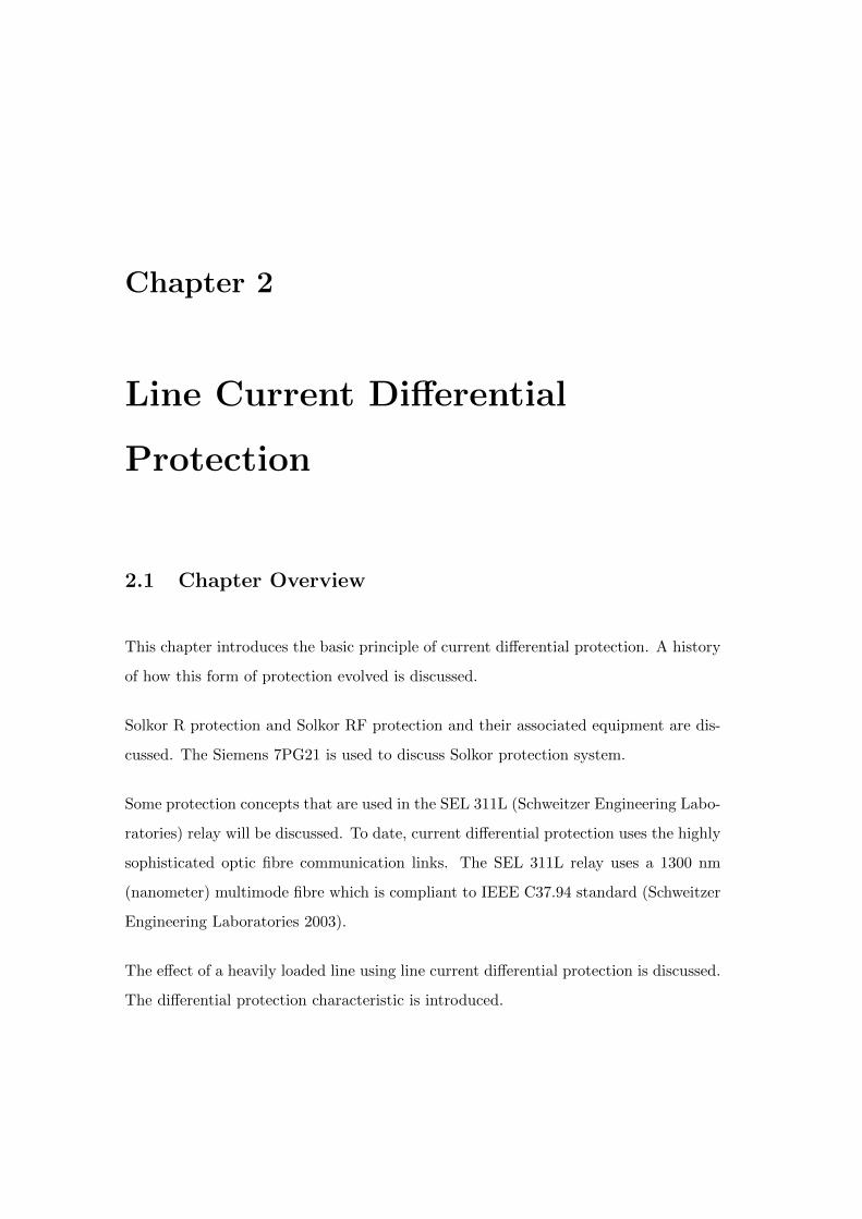
2.2 Principle of Line Current Differential Protection
The principle of current differential protection was first established by Merz and Price.
From then on, highly sophisticated current differential systems have been built (GEC
Alsthom 2011). Figure 2.1 shows the principle of a basic current differential scheme.
Current I is the load current shown flowing from left to right as shown by the arrow.
CT1 (current transformer 1) and CT2 (current transformer 2) are the two current
transformers connected in a differential mode. I1 and I2 are secondary currents from
the CTs. For a through fault, I1 and I2 will flow in the shown respective directions
and they will be equal in magnitude (Hewitson & Balakrishnan 2004).
According to Kirchoffs current law, the current flowing in the relay is given by:
IRelay = I1 − I2 (2.1)
For a through fault, I1 and I2 will be equal in magnitude and the result is that current
flows round the pilot loop and there will be zero current flowing in the relay hence no trip
will occur. If a fault exists at any point between the two CTs (current transformers),
Figure 2.1: Current differential Principle
Source: (Hewitson & Balakrishnan 2004)
then the two currents I1 and I2 will not sum to zero, instead a differential current is
created. This differential given by equation 2.1 flows in the relay. If the magnitude
of IRelay is greater than the relay setting, a trip will be issued at both ends of the
protected line.
On a 500 kV line, the CTs are not as close as shown in Figure 2.1. The distance
between the CTs could be tens or even hundreds of kilometres. In pilot wire systems,
2.3 Matched Current Transformers 6
there is a limit to the length of pilots that can be used on a protected line and this
limits the use of pilot wire protection on long feeders (Siemens 2012).
2.3 Matched Current Transformers
The CTs used for a 500 kV line current differential protection must be identical in
every respect. In reality this is not possible because some differences always exist. One
of these differences has something to do with remanence. This is the magnetic flux
that remains in a magnetic material after an applied magneto-motive force has been
removed.
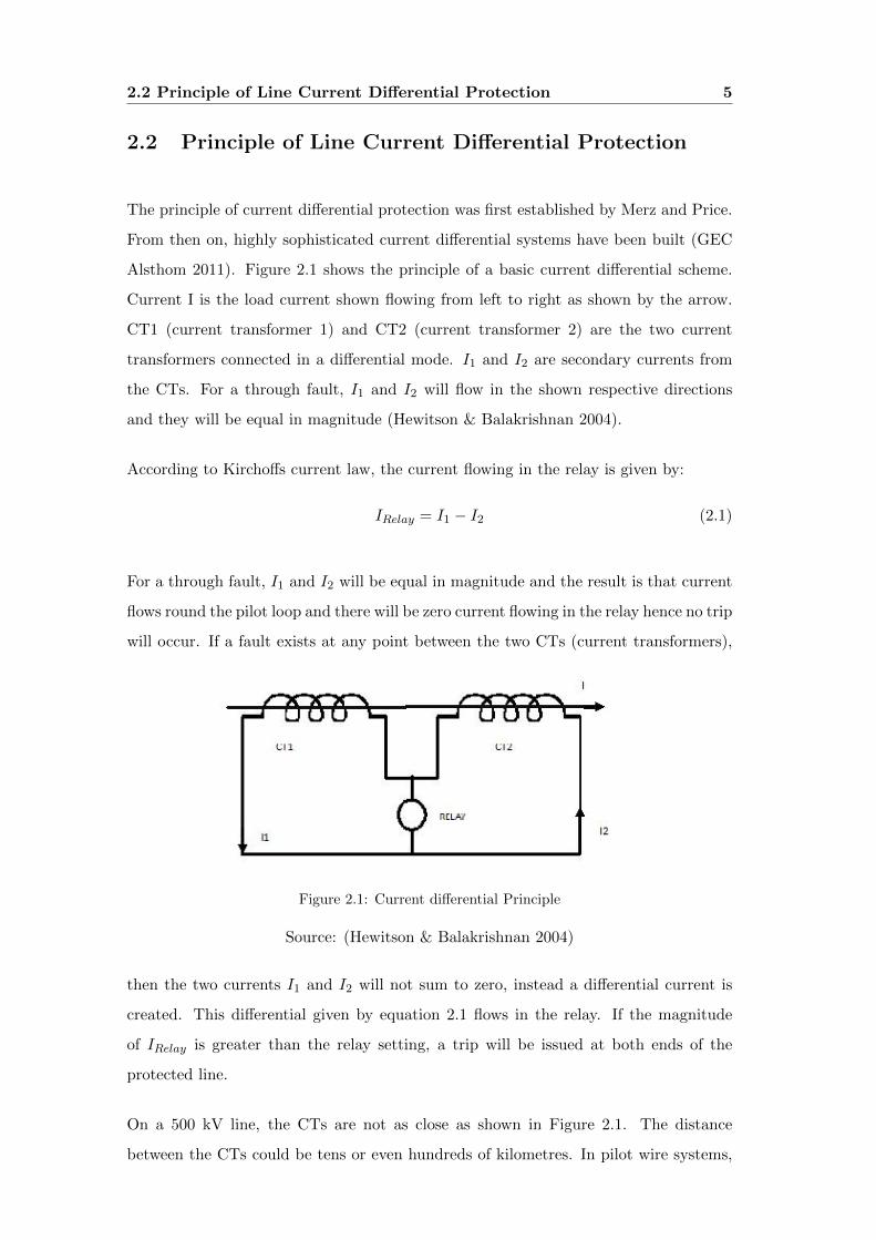
Mclaren & Jayasinghe (1997) carried out an experiment to explore the effect of re-
manence on CTs. They mentioned that CT secondary currents may be different for
the same primary current due to different levels of remanence in each CT. Mclaren &
Jayasinghe (1997) reported that the situation worsens when the primary current is high
and has a large exponential component whose time constant is 0.1 or greater.
Figure 2.2 shows the test circuit that was used to simulate CT remanence. It can be
noticed that the same current flows in the primary circuits of CT1 and CT2 and the
secondary circuits are connected in the differential mode.
Figure 2.2: Simulation Circuit
Source: (Mclaren & Jayasinghe 1997)
2.4 Pilot Wire Protection 7
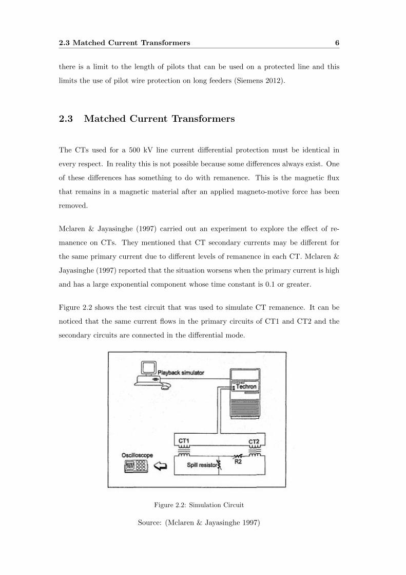
Work on a simulation of two CTs connected in parallel was carried out with an aim of
getting a comparison between test results and simulated results (Mclaren & Jayasinghe
1997). The interesting conclusion of Mclaren & Jayasinghe (1997) findings was that
there was significant spill current differences between an external fault and an internal
fault.
Figure 2.3: External Fault Simulation
Source: (Mclaren & Jayasinghe 1997)
The results of this experiment are shown in figure 2.3 where an external fault has been
simulated. It can be observed that the shape of the primary current is different from
that of the secondary. The difference in shape of the two current waveforms is caused
by remanence in the CT core material.
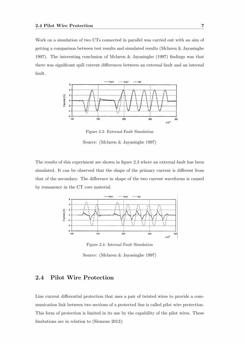
Figure 2.4: Internal Fault Simulation
Source: (Mclaren & Jayasinghe 1997)
2.4 Pilot Wire Protection
Line current differential protection that uses a pair of twisted wires to provide a com-
munication link between two sections of a protected line is called pilot wire protection.
This form of protection is limited in its use by the capability of the pilot wires. These
limitations are in relation to (Siemens 2012):
2.4 Pilot Wire Protection 8
• insulation resistance of the pilots.
• inter core capacitance of the pilot wires.
• loop resistance of the pilots.
In one form of pilot wire protection, CT secondary currents are wired as in figure 2.1 so
that no current flows in the relay for a through fault. This set up is known as circulating
current principle. In a voltage balance current differential protection, the CT secondary
circuits are cross connected so that no current flows in the series connected relays for
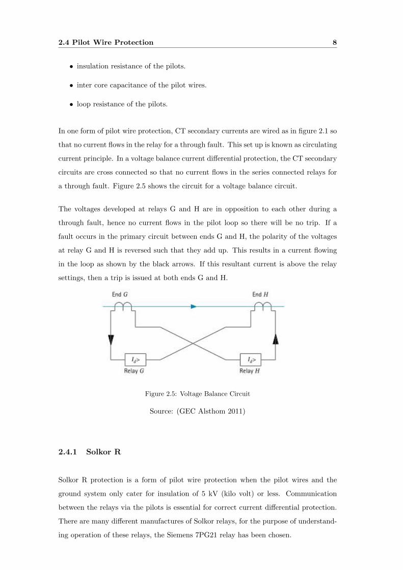
a through fault. Figure 2.5 shows the circuit for a voltage balance circuit.
The voltages developed at relays G and H are in opposition to each other during a
through fault, hence no current flows in the pilot loop so there will be no trip. If a
fault occurs in the primary circuit between ends G and H, the polarity of the voltages
at relay G and H is reversed such that they add up. This results in a current flowing
in the loop as shown by the black arrows. If this resultant current is above the relay
settings, then a trip is issued at both ends G and H.
Figure 2.5: Voltage Balance Circuit
Source: (GEC Alsthom 2011)
2.4.1 Solkor R
Solkor R protection is a form of pilot wire protection when the pilot wires and the
ground system only cater for insulation of 5 kV (kilo volt) or less. Communication
between the relays via the pilots is essential for correct current differential protection.
There are many different manufactures of Solkor relays, for the purpose of understand-
ing operation of these relays, the Siemens 7PG21 relay has been chosen.
2.4 Pilot Wire Protection 9
The Siemens 7PG21 is a typical Solkor protection relay which houses both R and RF
modes. It is equipped with an additional circuit that monitors the pilots. The pilot
supervision circuit is used to detect an open or short circuit on the pilots. An open
circuit on the pilots can cause a trip at both ends of the line while a short circuit
reduces the sensitivity of the relay (Siemens 2012).
2.4.2 Solkor RF
Solkor RF protection is a better version of the Solkor R protection and is used on
systems with either 5 kV or 15 kV insulation system. The Siemens RF version provides
faster clearing times of internal faults whilst the stability for through faults is the same
as Solkor R. Siemens 7PG21 relay offers both forms of protection namely R and RF.
Another advantage of the Siemens 7PG21 relay is that it can be used either in the R
mode or in the RF mode depending on the system requirements (Siemens 2012) . The
relay can be used in a 2 ended feeder of up to 20 km long and a maximum pilot loop
resistance of two thousand ohms .
Just like any relay design, the Siemens 7PG21 has requirements for CTs connected to
its inputs. ( Note: equation 2.2 is unique to the Siemens 7PG21 relay, different relays
have their own forms of this equation)
Vk =50
In+IFN
(RCT + 2RL) (2.2)
Where
• IF is the steady state fault current.
• In is the rated relay current.
• N is the CT ratio.
• RCT is the CT secondary resistance.
• RL is the lead resistance per phase between CT and the relay.
2.5 Summation Transformer for Pilot Wire Protection 10
Table 2.1: Siemens 7PG21 Relay Pilot Requirements (Siemens 2012)
R mode RF mode RF mode with 15 kV Trans
Tap1 Tap0.5 Tap0.25
Maximum loop resistance 1000Ω 2000Ω 1780Ω 880Ω 440Ω
Maximum Inter core Capacitance 2.5µF 0.8µF 1µF 2µF 4µF
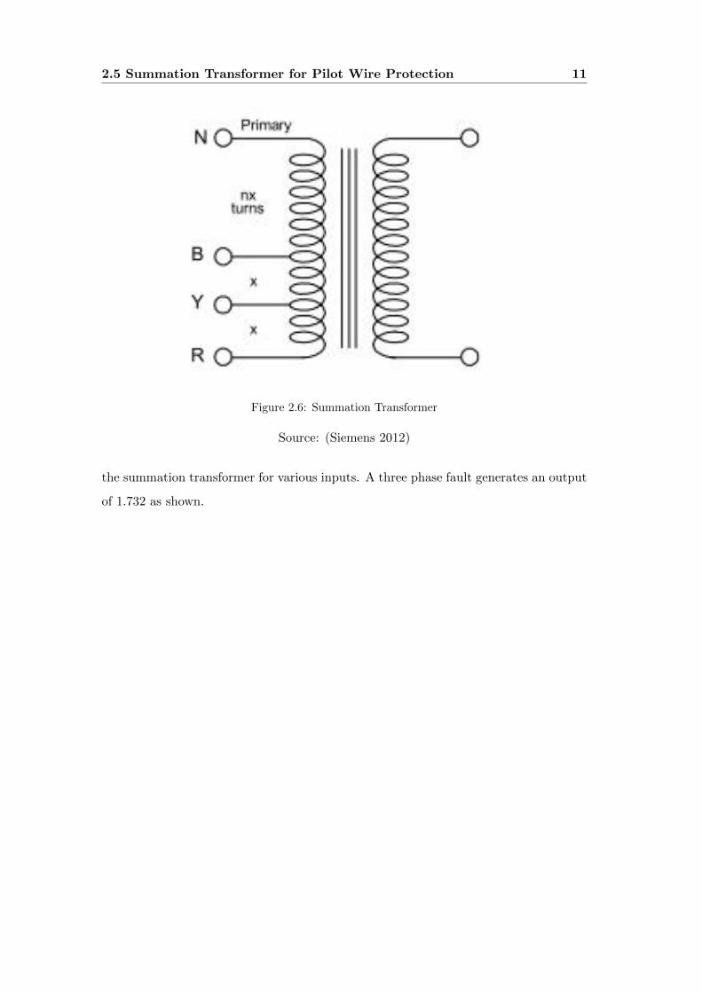
2.5 Summation Transformer for Pilot Wire Protection
The pilot circuits discussed so far use a summation transformer to sum the three phase
currents into an equivalent current single current that will flow in the two pilot wires.
Without the use of a summation transformer, six pilot wires would be needed in the
circuit with two pilots being used per phase. As can be seen, this would be uneconomic.
The summation transformer provides (Hacker 1998) :
• a reduction in secondary impedance as reflected in the primary winding by a
factor of k2 for a transformer with a ratio of 1:k , this is very advantageous in
that the CT burden is reduced.
• an insulation barrier between the CTs and the pilot circuitry.
• reduces the three phase circuitry to an equivalent single phase one, thus improves
economy on the pilot wires needed.
Use of the summation transformer makes it possible for the line differential protection
to compare various fault currents on a single phase basis over the two pilot wires
(Siemens 2012). Since the summation transformer provides insulation between CTs
and the pilots, the CTs can be earthed (at one point only) while there is no need to
then earth the pilots. Figure 2.6 shows the summation transformer where x represents
a multiplier in the taps.
The output of the summation transformer depends on the type of fault. Careful design
of the summation transformer tappings needs to be considered as zero output may
exist for complex faults on the primary. The knee point voltage of the summation
transformer needs to be high enough to accommodate maximum fault currents and the
dc offset without saturation as shown in equation 2.2. Table 2.2 shows the outputs of
2.5 Summation Transformer for Pilot Wire Protection 11
Figure 2.6: Summation Transformer
Source: (Siemens 2012)
the summation transformer for various inputs. A three phase fault generates an output
of 1.732 as shown.
2.5 Summation Transformer for Pilot Wire Protection 12
Table 2.2: Summation Transformer Outputs (Hacker 1998)
Comparative Output for equal fault currents Comparative Output for n equal 3
R - N n + 2 5
Y - N n + 1 4
B - N n 3
R - Y 1 1
Y - B 1 1
B - R 2 2
Three Phase 1.732 1.732
Table 2.3: Pilot Current and Voltage (Siemens 2012)
R mode RF mode RF mode with 15 kV Trans
Tap1 Tap0.5 Tap0.25
Peak pilot voltage during a fault 300v 450v 450v 350v 225v
Maximum pilot current during a fault 200mA 250mA 250mA 380mA 500mA
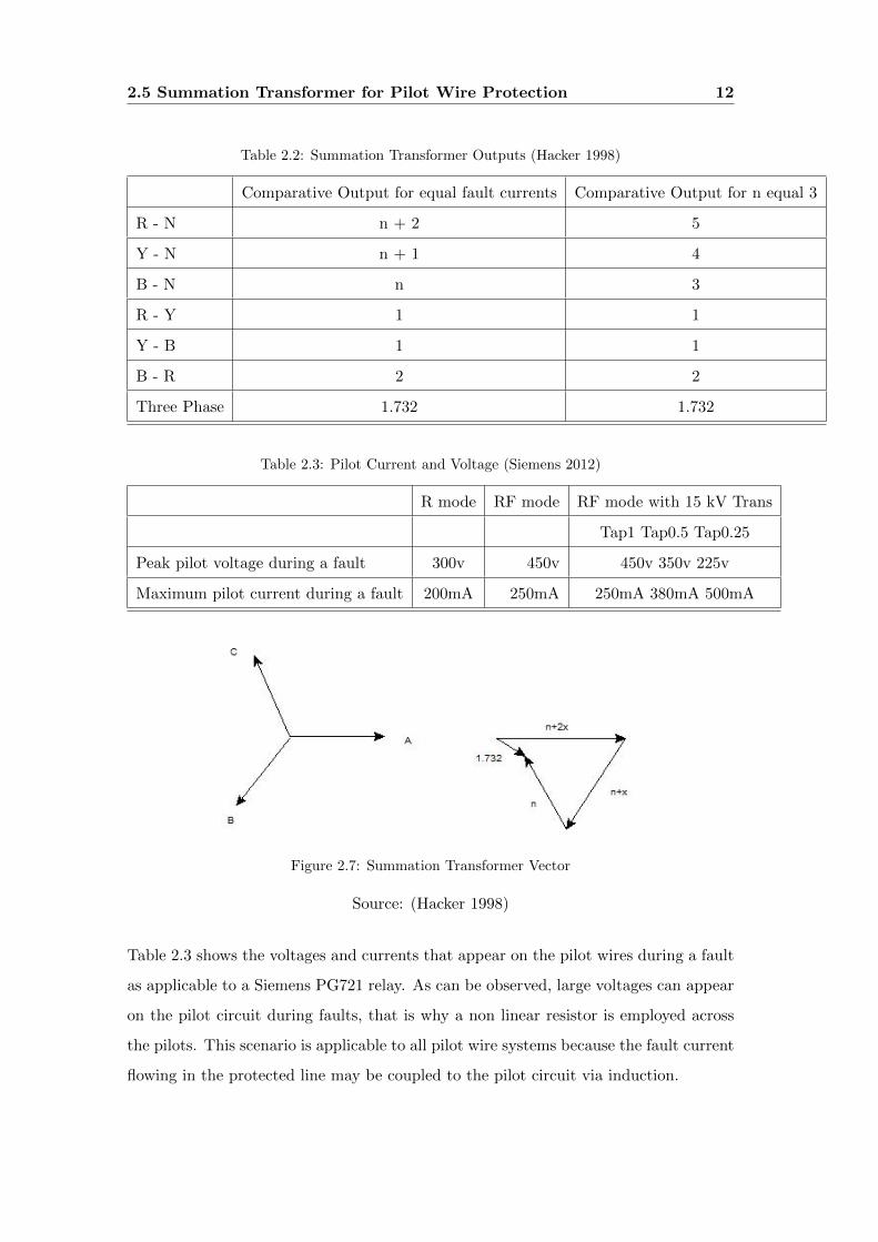
Figure 2.7: Summation Transformer Vector
Source: (Hacker 1998)
Table 2.3 shows the voltages and currents that appear on the pilot wires during a fault
as applicable to a Siemens PG721 relay. As can be observed, large voltages can appear
on the pilot circuit during faults, that is why a non linear resistor is employed across
the pilots. This scenario is applicable to all pilot wire systems because the fault current
flowing in the protected line may be coupled to the pilot circuit via induction.
2.6 Line differential Protection Characteristic 13
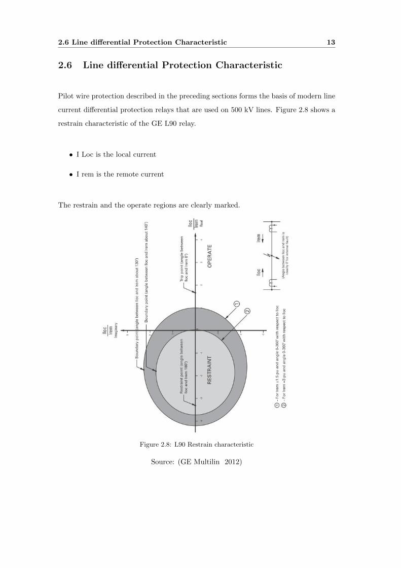
2.6 Line differential Protection Characteristic
Pilot wire protection described in the preceding sections forms the basis of modern line
current differential protection relays that are used on 500 kV lines. Figure 2.8 shows a
restrain characteristic of the GE L90 relay.
• I Loc is the local current
• I rem is the remote current
The restrain and the operate regions are clearly marked.
Figure 2.8: L90 Restrain characteristic
Source: (GE Multilin 2012)
2.7 A Heavily Loaded Line using Current Differential Protection 14
2.6.1 Copper Wire Communications Links
Communication in digital current differential protection is traditionally direct optic
fibre or multiplexed channels that use short copper links from the multiplexer to the
relay (Voloh & Johnson 2005). Some Utilities still use copper pilot wires as the com-
munication channel in their line current differential protection schemes.
Some of the major problems with implementing a 64 kbps (kilo bits per second) com-
munication link over copper wire are:
• noise.
• ground potential rise.
• lightning.
• induced voltages.
Suppose there happens to be a phase to ground fault at a local substation. A substan-
tial ground potential voltage rise may occur between the local and remote substation
grounds. This voltage rise presents stresses on the pilot wire relay and the pilot wires
themselves (Voloh & Johnson 2005). This can affect the proper operation of the pro-
tection.
2.7 A Heavily Loaded Line using Current Differential Pro-
tection
Line current differential protection measures the current through the protected line.
The differential protection then measures the difference in currents as seen by the
CTs at each end of the line. For a given load current through the protected line,
the currents measured at each end of the line are the same in magnitude hence the
differential current will be ideally zero. This means that a line current differential relay
will not trip on overload. This means that another relay that looks at the load current
has to be installed in order to prevent overloading the circuit.
However, the differential current measured by a line current differential relay increases
2.7 A Heavily Loaded Line using Current Differential Protection 15
with load. In other words, the difference in measured current is a constant for a given
load on the line. This means that as the load increases, the difference current also
increases accordingly. To avoid errors some relays have two slopes on their differential
relay characteristic.
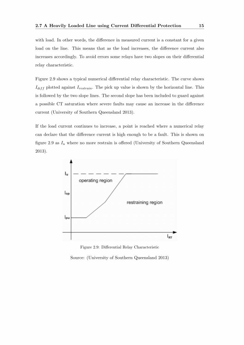
Figure 2.9 shows a typical numerical differential relay characteristic. The curve shows
Idiff plotted against Irestrain. The pick up value is shown by the horizontal line. This
is followed by the two slope lines. The second slope has been included to guard against
a possible CT saturation where severe faults may cause an increase in the difference
current (University of Southern Queensland 2013).
If the load current continues to increase, a point is reached where a numerical relay
can declare that the difference current is high enough to be a fault. This is shown on
figure 2.9 as Iu where no more restrain is offered (University of Southern Queensland
2013).
Figure 2.9: Differential Relay Characteristic
Source: (University of Southern Queensland 2013)
2.8 Current Differential Protection in Teed Lines 16
Table 2.4: SEL 311L Relay in a 3 Way Loop (Schweitzer Engineering Laboratories 2003)
1 2 3
IRemote IL+IS IR+IS IR+IR
ILocal IR IL IS
2.8 Current Differential Protection in Teed Lines
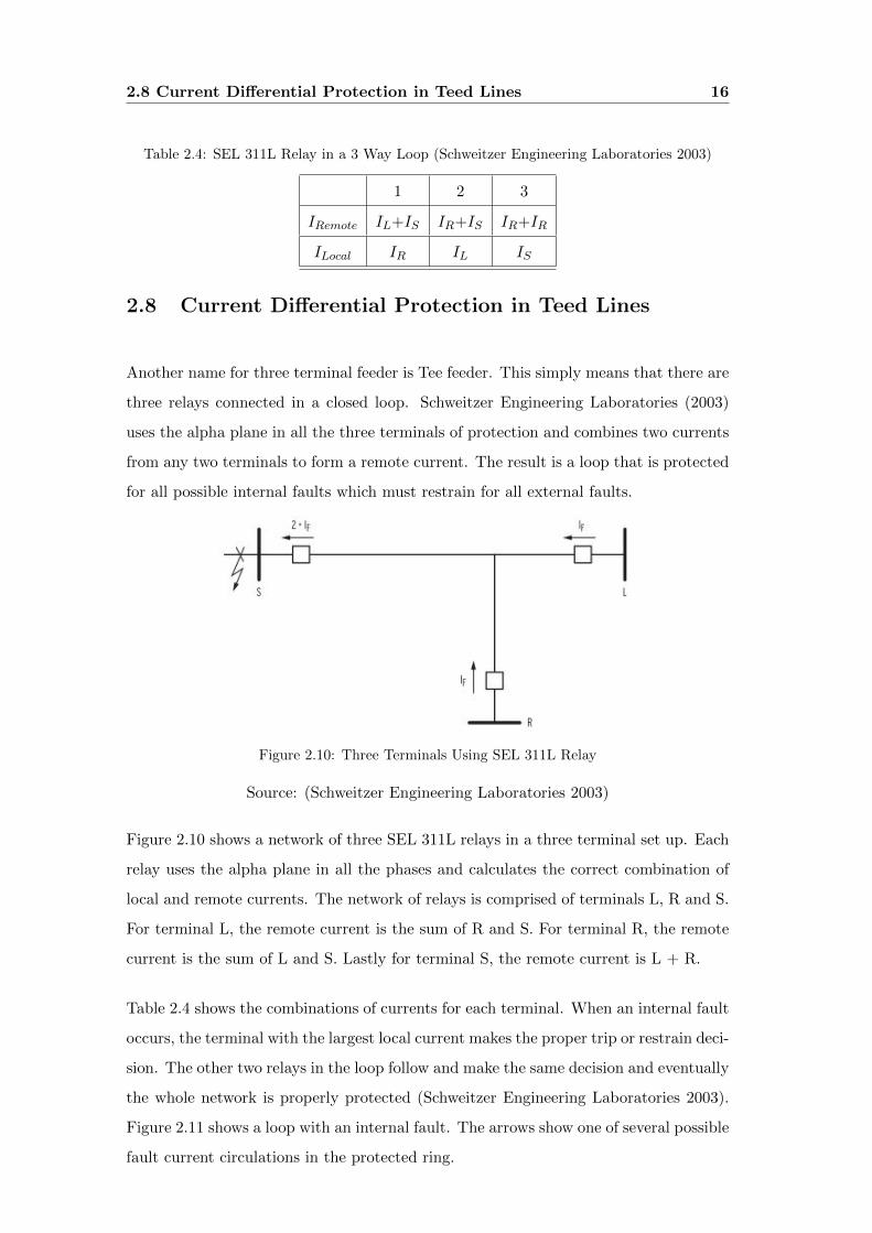
Another name for three terminal feeder is Tee feeder. This simply means that there are
three relays connected in a closed loop. Schweitzer Engineering Laboratories (2003)
uses the alpha plane in all the three terminals of protection and combines two currents
from any two terminals to form a remote current. The result is a loop that is protected
for all possible internal faults which must restrain for all external faults.
Figure 2.10: Three Terminals Using SEL 311L Relay
Source: (Schweitzer Engineering Laboratories 2003)
Figure 2.10 shows a network of three SEL 311L relays in a three terminal set up. Each
relay uses the alpha plane in all the phases and calculates the correct combination of
local and remote currents. The network of relays is comprised of terminals L, R and S.
For terminal L, the remote current is the sum of R and S. For terminal R, the remote
current is the sum of L and S. Lastly for terminal S, the remote current is L + R.
Table 2.4 shows the combinations of currents for each terminal. When an internal fault
occurs, the terminal with the largest local current makes the proper trip or restrain deci-
sion. The other two relays in the loop follow and make the same decision and eventually
the whole network is properly protected (Schweitzer Engineering Laboratories 2003).
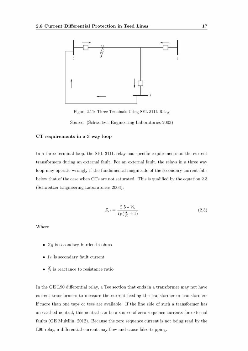
Figure 2.11 shows a loop with an internal fault. The arrows show one of several possible
fault current circulations in the protected ring.
2.8 Current Differential Protection in Teed Lines 17
Figure 2.11: Three Terminals Using SEL 311L Relay
Source: (Schweitzer Engineering Laboratories 2003)
CT requirements in a 3 way loop
In a three terminal loop, the SEL 311L relay has specific requirements on the current
transformers during an external fault. For an external fault, the relays in a three way
loop may operate wrongly if the fundamental magnitude of the secondary current falls
below that of the case when CTs are not saturated. This is qualified by the equation 2.3
(Schweitzer Engineering Laboratories 2003):
ZB =2.5 ∗ VSIF (XR + 1)
(2.3)
Where
• ZB is secondary burden in ohms
• IF is secondary fault current
• XR is reactance to resistance ratio
In the GE L90 differential relay, a Tee section that ends in a transformer may not have
current transformers to measure the current feeding the transformer or transformers
if more than one taps or tees are available. If the line side of such a transformer has
an earthed neutral, this neutral can be a source of zero sequence currents for external
faults (GE Multilin 2012). Because the zero sequence current is not being read by the
L90 relay, a differential current may flow and cause false tripping.
2.8 Current Differential Protection in Teed Lines 18
To solve the problem GE Multilin (2012) removes the zero sequence current from the
phase currents before they generate a differential current. This improves stability for
external faults whilst enforcing a trip for internal faults.
2.9 Chapter Summary 19
2.9 Chapter Summary
This chapter introduced current differential protection from its early form which was
called pilot wire protection to the latest versions which now use fibre optical links to
communicate to the remote end of the line.
Pilot wire protection has a limitation in the length of pilot wires that can be used.
There is also a limitation in the loop resistance of the pilot circuit.
Capacitance of the pilot wires limits the use of pilot wire protection when longer lines
are involved. Capacitance of pilot wires tends to reduce sensitivity of the protection if
it is of the current difference protection type but causes tripping if the protection is of
the opposed voltage type.
A typical line current differential protection characteristic of the GE L90 relay was
presented. The local and remote currents are shown on the characteristic.
Chapter 3
Distance Protection
3.1 Chapter Overview
In this chapter, distance protection is introduced. Typical characteristics and zones of
protection are explained. Timing of zones of protection is covered in section 3.2 . A
discussion of distance protection in a Teed line is covered in section 3.4 A problem that
may manifest itself in distance protection is load encroachment. This is dealt with in
section 3.6 Unstable situations may happen on a power system. Distance protection
power swing feature can detect such instabilities. This concept is looked at in section
3.7. Protection schemes related to distance protection are introduced in section 3.8
3.2 What is Distance Protection
Distance protection is a form of protection where the impedance of the protected section
is measured. If the apparent impedance seen by the relay falls below the setting, a
distance relay registers a fault and a trip is initiated. Distance protection is directional
and is a non unit form of protection. It is very fast in operation for faults along most
part of the protected line.
Because the impedance of a transmission line is proportional to its length, the distance
relay is able to measure impedance of a line up to a pre-determined point called the
reach point. In this way, a distance relay is able to differentiate faults that occur
3.2 What is Distance Protection 21
between the relaying point and the reach point, and faults that can occur beyond the
reach point (GEC Alsthom 2011).
A distance relay measures voltage and current flowing in a transmission line. The
measured voltage is divided by the measured current to give an impedance called an
apparent impedance. If this apparent impedance is less than a reach point impedance,
it is assumed that a fault has occurred between the relaying point and the reach point.
An under reaching protection is a form of protection that will not see faults beyond
a certain point. An overreaching protection is that protection which will see faults
beyond a certain point (Horowitz & Phadke 2009) .
A distance relay does not measure the line impedance directly but uses an indirect
method. It achieves this by measuring the voltages and currents, then it calculates
impedance from these quantities.
3.2.1 Relay Performance
The performance of a distance relay is determined by measuring how accurate a given
relay achieves the set trip times and how accurate the relay measures impedance. The
reach accuracy depends on:
• the voltage applied to the relay during a fault.
• impedance measuring techniques used in the relay design.
Operating times of a relay vary with the fault current, the fault position relative to
the relay setting and also with the point on wave at which the fault occurs (GEC
Alsthom 2011) . As can be noted from the foregoing discussion, it is evident that a delay
in the operation of the relay is inevitable. The time delay in relay operation for faults
close to reach point can be caused by things such as measured signal transient errors
caused by capacitor voltage transformers (CVTs) and saturated current transformers
(CTs).
Because of this variation in operating times, relay manufactures usually quote max-
imum and minimum values. Electromechanical relays have a larger operating time
3.2 What is Distance Protection 22
variation than their digital and numeric counterparts over a wide range of system op-
erating conditions and fault positions. A systematic procedure to determine distance
protection settings, seeks to look at a relay with minimum variation of operating time
and minimum errors in reach accuracy. This project is aiming at achieving the deter-
mination of relay settings then a simulation of faults will be carried out to see if the
relay performs according to the expected criteria.
Figure 3.1 shows the variation of zone 1 reach impedance for varying percentages of
rated voltage. Part (a) shows the behaviour for phase to earth faults, part (b) shows
the behaviour for phase to phase faults and part (c) shows the behaviour in three phase
faults (GEC Alsthom 2011) . There is a more flat response in parts (b) and (c) whereas
in part (a), the plot shows an ever increasing effect for increase in voltage and it then
becomes flat at 60% of rated voltage. An ideal relay is one whose response curve would
stay flat at 100% reach setting for any voltage up to rated voltage.
Figure 3.1: Impedance Reach Accuracy
Source: (GEC Alsthom 2011)
3.3 Zones of Protection 23
Figure 3.2 shows the variation of operating time with relation to the fault position for
particular system impedance ratios. System impedance ratio is defined by equation 3.1
SIR =ZSZL
(3.1)
where
• SIR is system impedance ratio
• ZS is source impedance behind the relay
• ZL is the line impedance
Figure 3.2: Trip Time versus fault position
Source: (GEC Alsthom 2011)
3.3 Zones of Protection
A basic distance relay has an instantaneous zone 1 and one or more time delayed zones.
Numeric relays can have up to six zones of protection with some of them set to look in
3.3 Zones of Protection 24
reverse. To determine settings for a particular scheme, a chosen relay manufacturer’s
relay instruction manual has to be consulted.
Figure 3.3 shows the three zones of protection. These are zones 1,2 and 3. All the shown
zones are forward looking. Relay Rab looks from A towards B along line AB, similarly
relay Rba looks towards A from end B. Zone 1 typically covers 80 percent of the line
between points A and B. This is because errors occur in calculating line parameters,
there are errors in CT and VT ratios. So in order to make sure the protection trips
only for faults between A and B, an under reach of point B by 20 percent is effected
on the relay setting so that zone 1 definitely trips instantaneously for faults between A
and B.
Zone 2 of line AB covers the remaining 10 percent of line AB plus an extra 20 percent
reach into an adjacent line BC. Zone 2 has a time delay of typically 400 mS to allow
for zone 1 of line BC to trip first. Zone 3 is another back up zone for line AB and it
has a time delay higher than that of zone 2. The zone of protection of a distance relay
is open at the far end. This means that the remote reach point cannot be precisely
measured (Horowitz & Phadke 2009).
Figure 3.3: Zones of Protection
Source: (Horowitz & Phadke 2009)
3.3.1 Zone 1
In electromechanical relays, zone 1 is set to cover 80% of the protected line. Numeric
relays can be set to cover up to 85% of the protected line. This is because digital and
numeric relays are more accurate and precise hence the 15% safe margin is good. The
reason for excluding this 15% portion of the line in zone 1 is because of:
• current transformer errors.
3.3 Zones of Protection 25
• voltage transformer errors.
• inaccuracies in line data.
• relay setting and measurement errors (GEC Alsthom 2011) .
The 15% impedance margin helps to maintain discrimination with the fast protection
of the next adjacent line. Zone 2 covers the remaining 15% of the protected line and
some portion of the next adjacent line (GEC Measurements 1984) . The operating time
of zone 1 is theoretically zero seconds, in reality this is around 20 mS (milliseconds)
depending on relay manufacturer. The author has tested a BBC L8a electromechanical
distance relay and the zone 1 operating time is typically 17 mS, far outclassing a GEC
Alsthom numeric relay LFZR111 which would give operating times of about 32 mS for
the same fault.
3.3.2 Zone 1 Extension
When used, zone 1 extension is set to 150% zone 1 reach. Zone 1 extension does
not need a signalling channel (GEC Measurements 1984) . Ideally zone 1 extension is
extending zone 1 reach so that most faults on the line will trip in zone 1 time. This
means that any initial fault in such a scheme will operate in zone 1 time, then after the
first trip and a re-closure, the re-closing equipment is used to reset the zone 1 extension
so that during the second trip (if the fault persists) individual zones become available
independently. After a complete trip and re-close cycle, even up to lockout, zone 1
extension is made available again.
On a 500 kV line, zone 1 extension is seldom used. Unit protection such as current dif-
ferential is the main protection while distance protection is used as back up protection.
In some cases both distance and current differential protections can be enabled at the
same time. Zone 1 extension is mainly used in sub-transmission or distribution radial
lines. The author has commissioned a GEC Quadramho relay with zone 1 extension
on an 88 kV radial feeder.
3.3 Zones of Protection 26
3.3.3 Zone 2
Zone 2 setting should be set at minimum 120% of the line impedance. The 20%
impedance above the reach point value is set so that it becomes definitely known that
zone 2 covers the whole line length. In many applications, zone 2 is set to cover 100%
of a protected line plus 50% of the shortest adjacent line. Zone 2 operation is time
delayed so that grading is achieved between zones 1 and 2 of adjacent line sections
(GEC Alsthom 2011) . This means that a given line is totally protected, having fast
clearance of faults in the first 80% to 85% of the line and slower clearance of faults in
the remaining section of the line.
3.3.4 Zone 3
Zone 3 is a zone that provides back up protection for the adjacent line sections. It is
time delayed to discriminate zone 3 with zone 2. In some installations, zone 3 is set
to have some reverse reach so that it provides back up protection behind the relaying
point. Zone 3 is thus set to 130% of the protected line plus the longest second line.
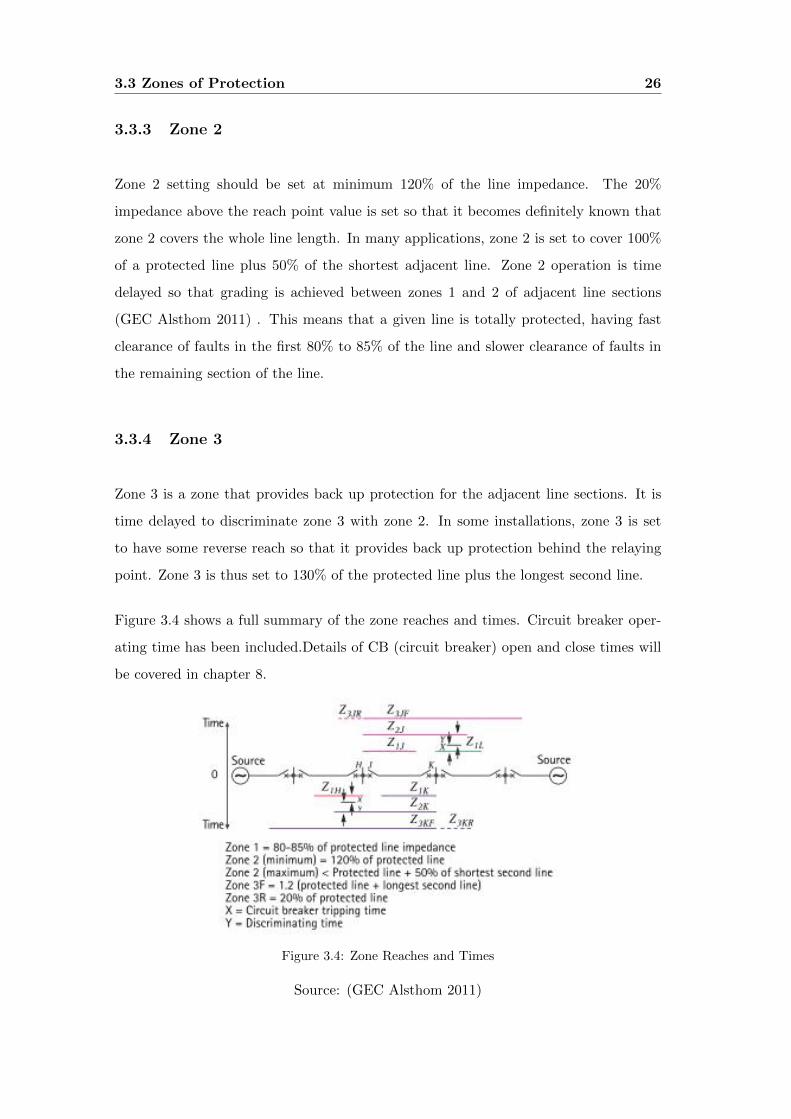
Figure 3.4 shows a full summary of the zone reaches and times. Circuit breaker oper-
ating time has been included.Details of CB (circuit breaker) open and close times will
be covered in chapter 8.
Figure 3.4: Zone Reaches and Times
Source: (GEC Alsthom 2011)
3.4 Characteristics 27
3.4 Characteristics
A distance relay has two main operating characteristics. These are the quadrilateral
and mho characteristics. As the name suggests, a quadrilateral characteristics is shaped
in the form of a quadrilateral. The mho characteristics is shaped in the form of a circle.
The resistance of the 500 kV line is plotted along the x axis and the reactance of the
500 kV line is plotted along the y axis or the j axis.
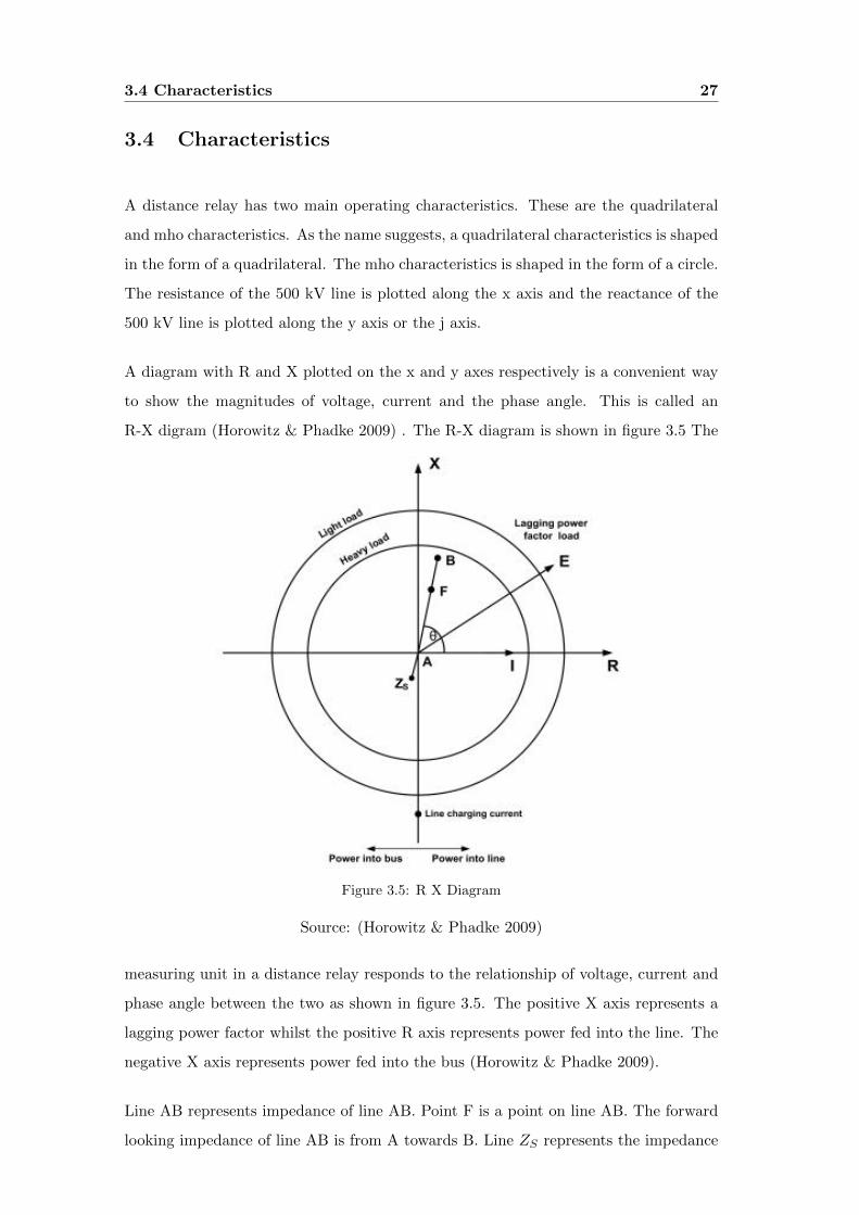
A diagram with R and X plotted on the x and y axes respectively is a convenient way
to show the magnitudes of voltage, current and the phase angle. This is called an
R-X digram (Horowitz & Phadke 2009) . The R-X diagram is shown in figure 3.5 The
Figure 3.5: R X Diagram
Source: (Horowitz & Phadke 2009)
measuring unit in a distance relay responds to the relationship of voltage, current and
phase angle between the two as shown in figure 3.5. The positive X axis represents a
lagging power factor whilst the positive R axis represents power fed into the line. The
negative X axis represents power fed into the bus (Horowitz & Phadke 2009).
Line AB represents impedance of line AB. Point F is a point on line AB. The forward
looking impedance of line AB is from A towards B. Line ZS represents the impedance
3.4 Characteristics 28
behind the relaying point A. This impedance is called the source impedance behind
the relay. Varying quantities of load currents are represented by circles of different
radii concentric about point A. The point on the negative X axis labelled line charging
current is of special interest in this project.
Line charging current is brought about because there is capacitance associated with a
500 kV line. In distribution networks, this capacitance is so small that its significance
can be ignored. However the situation is completely different when it comes to a 500
kV line. The capacitance is quite large such that it causes a capacitive current to flow
in the line. This capacitance causes the apparent impedance seen by a relay to change
if it is ignored in the relay setting calculation process.
It is good to see that in figure 3.5, the line charging current is outside the relay char-
acteristic during light loading conditions. This means that line charging capacitance
although available, it is not interfering with the relay operation. In situations where
line charging current enters the operating characteristics of the relay, then compensa-
tion for this current has to be done. The effect of line capacitance on relay setting is
covered in chapter 5.
3.4.1 Mho Characteristic
The mho is a unit of measurement which represents the inverse or resistance. The unit
can also be called Siemens. The characteristics of a mho element when plotted on an
R-X diagram is a circle which passes through the origin (GEC Alsthom 2011) . This
means that a mho element is inherently directional and as such it can be used in the
distance relay to give a directional characteristic.
The impedance characteristic can be adjusted by setting the impedance reach along
the diameter of the circle. The diameter is displaced at an angle φ to the positive R
axis (the x axis), this angle is known as the relay characteristic angle.
3.4.2 Quadrilateral Characteristic
Figure 3.6 shows an R-X diagram that shows the relationship between voltage,current
and phase angle as measured by a distance relay. In this diagram point A is the origin.
3.5 Distance Protection in Parallel Lines 29
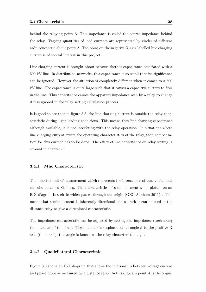
B and C are points on the line. Rz1, Rz2 and Rz3 are the resistive reaches of the line.
Angle CAR is the line characteristic angle. In Figure 3.6 Zone 3 is forward looking but
it has some reverse reach (GEC Measurements 1984)
Figure 3.6: Quadrilateral Characteristic
Source: (GEC Measurements 1984)
3.5 Distance Protection in Parallel Lines
3.6 Teed Feeders
3.7 Distance Protection in a Heavily Loaded Line
Figure 3.5 shows two circles whose origin is at point A. The inner circle with a smaller
radius represents impedance of a heavy load. This is because a distance relay calculates
impedance using the Ohm’s law equation:
zph =vphIph
(3.2)
If the load current increases, zph gets smaller. Horowitz & Phadke (2009) discusses the
effect that the load current has on the characteristics of a distance relay. For some
value of line load, the apparent impedance seen by a distance relay may cross into a
zone of operation of the relay (usually zone 3), the relay will trip in zone 3 time. The
3.7 Distance Protection in a Heavily Loaded Line 30
load MVA at which this happens is called the load-ability limit of the relay (Horowitz
& Phadke 2009).
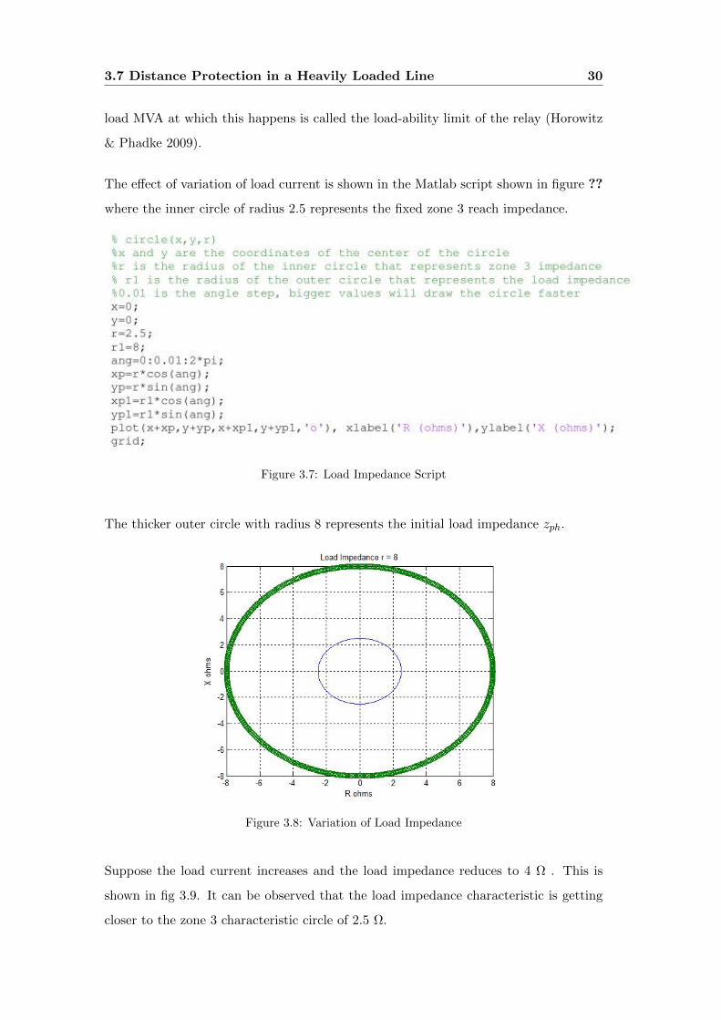
The effect of variation of load current is shown in the Matlab script shown in figure ??
where the inner circle of radius 2.5 represents the fixed zone 3 reach impedance.
Figure 3.7: Load Impedance Script
The thicker outer circle with radius 8 represents the initial load impedance zph.
Figure 3.8: Variation of Load Impedance
Suppose the load current increases and the load impedance reduces to 4 Ω . This is
shown in fig 3.9. It can be observed that the load impedance characteristic is getting
closer to the zone 3 characteristic circle of 2.5 Ω.
3.7 Distance Protection in a Heavily Loaded Line 31
Figure 3.9: Variation of Load Impedance
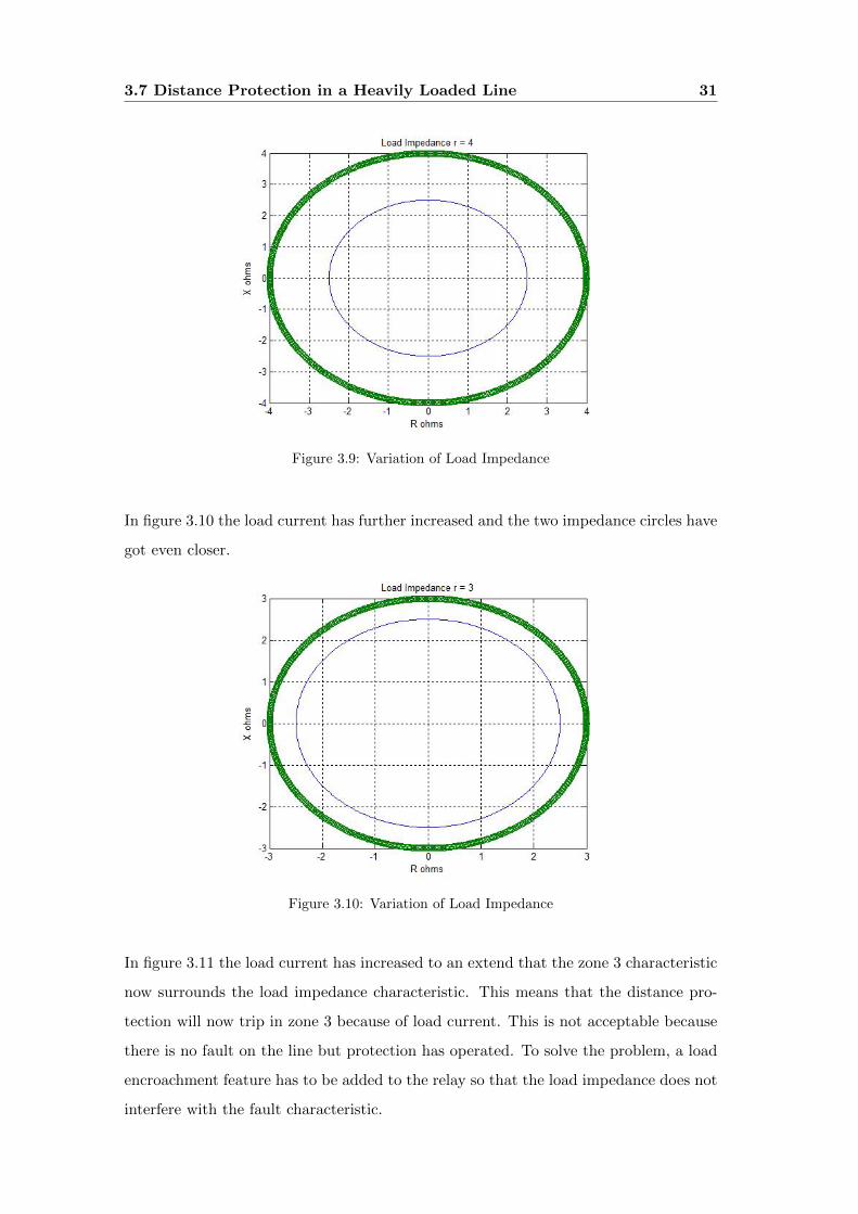
In figure 3.10 the load current has further increased and the two impedance circles have
got even closer.
Figure 3.10: Variation of Load Impedance
In figure 3.11 the load current has increased to an extend that the zone 3 characteristic
now surrounds the load impedance characteristic. This means that the distance pro-
tection will now trip in zone 3 because of load current. This is not acceptable because
there is no fault on the line but protection has operated. To solve the problem, a load
encroachment feature has to be added to the relay so that the load impedance does not
interfere with the fault characteristic.
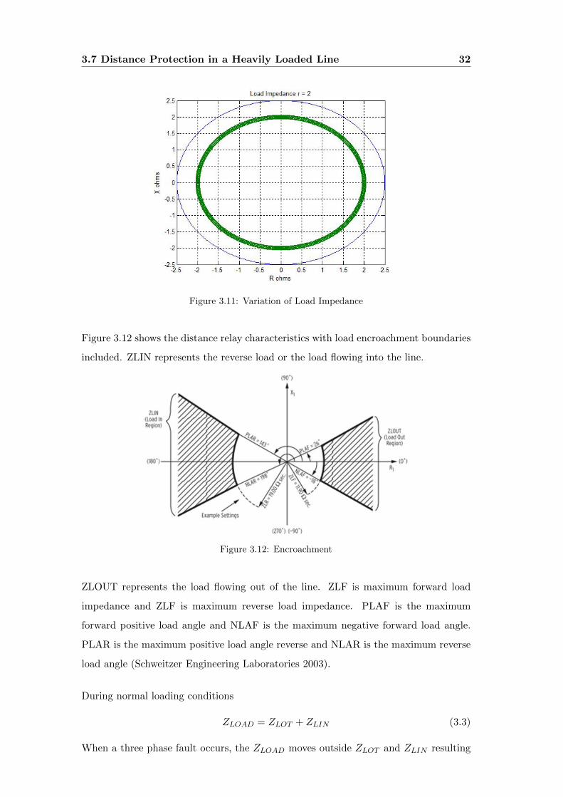
3.7 Distance Protection in a Heavily Loaded Line 32
Figure 3.11: Variation of Load Impedance
Figure 3.12 shows the distance relay characteristics with load encroachment boundaries
included. ZLIN represents the reverse load or the load flowing into the line.
Figure 3.12: Encroachment
ZLOUT represents the load flowing out of the line. ZLF is maximum forward load
impedance and ZLF is maximum reverse load impedance. PLAF is the maximum
forward positive load angle and NLAF is the maximum negative forward load angle.
PLAR is the maximum positive load angle reverse and NLAR is the maximum reverse
load angle (Schweitzer Engineering Laboratories 2003).
During normal loading conditions
ZLOAD = ZLOT + ZLIN (3.3)
When a three phase fault occurs, the ZLOAD moves outside ZLOT and ZLIN resulting
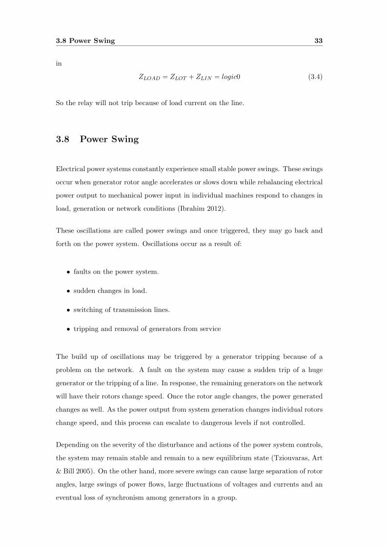
3.8 Power Swing 33
in
ZLOAD = ZLOT + ZLIN = logic0 (3.4)
So the relay will not trip because of load current on the line.
3.8 Power Swing
Electrical power systems constantly experience small stable power swings. These swings
occur when generator rotor angle accelerates or slows down while rebalancing electrical
power output to mechanical power input in individual machines respond to changes in
load, generation or network conditions (Ibrahim 2012).
These oscillations are called power swings and once triggered, they may go back and
forth on the power system. Oscillations occur as a result of:
• faults on the power system.
• sudden changes in load.
• switching of transmission lines.
• tripping and removal of generators from service
The build up of oscillations may be triggered by a generator tripping because of a
problem on the network. A fault on the system may cause a sudden trip of a huge
generator or the tripping of a line. In response, the remaining generators on the network
will have their rotors change speed. Once the rotor angle changes, the power generated
changes as well. As the power output from system generation changes individual rotors
change speed, and this process can escalate to dangerous levels if not controlled.
Depending on the severity of the disturbance and actions of the power system controls,
the system may remain stable and remain to a new equilibrium state (Tziouvaras, Art
& Bill 2005). On the other hand, more severe swings can cause large separation of rotor
angles, large swings of power flows, large fluctuations of voltages and currents and an
eventual loss of synchronism among generators in a group.
3.8 Power Swing 34
Tziouvaras et al. (2005) mentions that large power swings stable or unstable can cause
unwanted relay operations at different network locations and this can lead to cascading
outages and possible blackouts. The equation that governs the power delivered by a
generator is given by (Grainger & Stevenson 1994):
P =E ∗ V ∗ sinδ
X(3.5)
Where
• P is the power generated.
• E is the generated electromotive force (emf).
• V is the terminal voltage.
• δ is the angle between E and V.
• X is the machine reactance
Equation 3.5 indicates that any change in E, V or δ can cause P to change. If the
change in P is too drastic, a power swing in a network occurs.
Power swing can cause the load impedance (which is usually out of the operating zone
characteristics of a distance relay) to enter the operating characteristics of a distance
relay. The relay may then operate and once a major load is removed from the system,
a power swing defined by equation 3.5 then results and the system becomes unstable.
An example of a power swing is given by (Ibrahim 2012) where symmetrical components
of a fault were played back and the readings were V1 = 36 6 98.8 volts, I1 = 6.3 6 54.5
amps, V2 = 0.5 volts, I2 = 0.2 amps, V0 = 0.1 volts, I0 = 0 amps. The resulting positive
sequence impedance is given by V1/I1 to give 366 98.8/6.36 54.5 = 5.76 43.3 ohms.
The zone 1 impedance of the protected line is 8.1 6 60. It can be observed that the power
swing impedance vector went straight into zone 1 operating characteristic resulting in
a trip in zone 1 time. Another thing observed is example is that there were very little
zero sequence components. This is usually the case with power swings, a power swing
is mostly a three (3) phase phenomena. This also explains why there was very little
negative sequence components in the fault records.
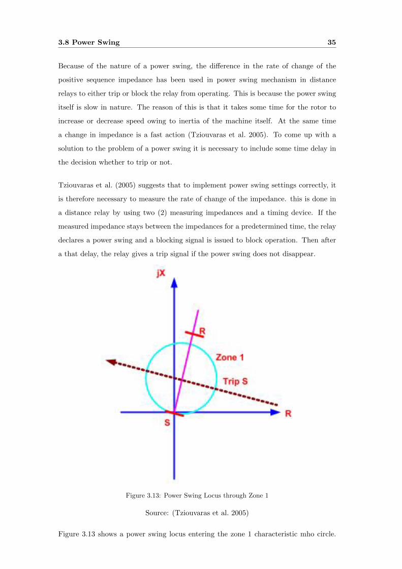
3.8 Power Swing 35
Because of the nature of a power swing, the difference in the rate of change of the
positive sequence impedance has been used in power swing mechanism in distance
relays to either trip or block the relay from operating. This is because the power swing
itself is slow in nature. The reason of this is that it takes some time for the rotor to
increase or decrease speed owing to inertia of the machine itself. At the same time
a change in impedance is a fast action (Tziouvaras et al. 2005). To come up with a
solution to the problem of a power swing it is necessary to include some time delay in
the decision whether to trip or not.
Tziouvaras et al. (2005) suggests that to implement power swing settings correctly, it
is therefore necessary to measure the rate of change of the impedance. this is done in
a distance relay by using two (2) measuring impedances and a timing device. If the
measured impedance stays between the impedances for a predetermined time, the relay
declares a power swing and a blocking signal is issued to block operation. Then after
a that delay, the relay gives a trip signal if the power swing does not disappear.
Figure 3.13: Power Swing Locus through Zone 1
Source: (Tziouvaras et al. 2005)
Figure 3.13 shows a power swing locus entering the zone 1 characteristic mho circle.
3.9 Distance Protection Schemes 36
The power swing locus is the brown dotted arrow labelled Trip S.
3.9 Distance Protection Schemes
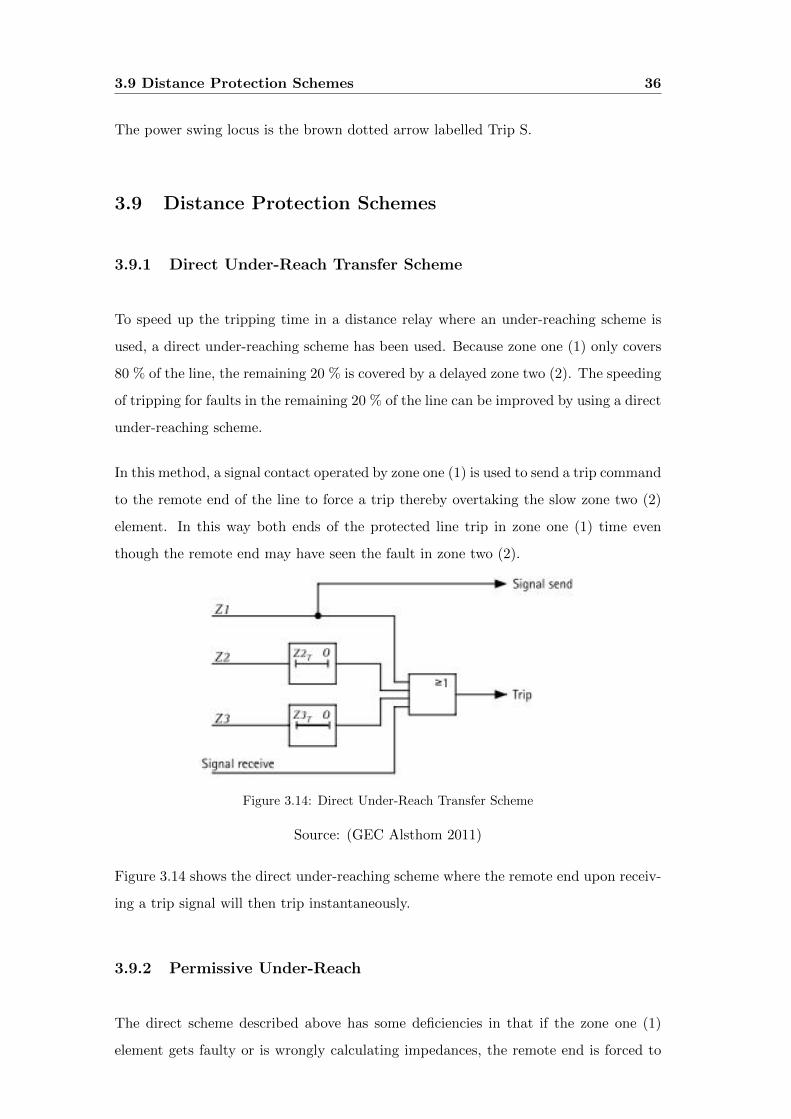
3.9.1 Direct Under-Reach Transfer Scheme
To speed up the tripping time in a distance relay where an under-reaching scheme is
used, a direct under-reaching scheme has been used. Because zone one (1) only covers
80 % of the line, the remaining 20 % is covered by a delayed zone two (2). The speeding
of tripping for faults in the remaining 20 % of the line can be improved by using a direct
under-reaching scheme.
In this method, a signal contact operated by zone one (1) is used to send a trip command
to the remote end of the line to force a trip thereby overtaking the slow zone two (2)
element. In this way both ends of the protected line trip in zone one (1) time even
though the remote end may have seen the fault in zone two (2).
Figure 3.14: Direct Under-Reach Transfer Scheme
Source: (GEC Alsthom 2011)
Figure 3.14 shows the direct under-reaching scheme where the remote end upon receiv-
ing a trip signal will then trip instantaneously.
3.9.2 Permissive Under-Reach
The direct scheme described above has some deficiencies in that if the zone one (1)
element gets faulty or is wrongly calculating impedances, the remote end is forced to
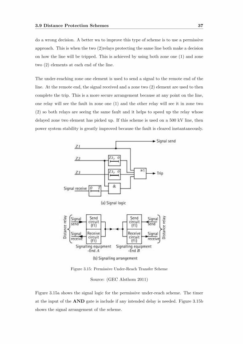
3.9 Distance Protection Schemes 37
do a wrong decision. A better wa to improve this type of scheme is to use a permissive
approach. This is when the two (2)relays protecting the same line both make a decision
on how the line will be tripped. This is achieved by using both zone one (1) and zone
two (2) elements at each end of the line.
The under-reaching zone one element is used to send a signal to the remote end of the
line. At the remote end, the signal received and a zone two (2) element are used to then
complete the trip. This is a more secure arrangement because at any point on the line,
one relay will see the fault in zone one (1) and the other relay will see it in zone two
(2) so both relays are seeing the same fault and it helps to speed up the relay whose
delayed zone two element has picked up. If this scheme is used on a 500 kV line, then
power system stability is greatly improved because the fault is cleared instantaneously.
Figure 3.15: Permissive Under-Reach Transfer Scheme
Source: (GEC Alsthom 2011)
Figure 3.15a shows the signal logic for the permissive under-reach scheme. The timer
at the input of the AND gate is include if any intended delay is needed. Figure 3.15b
shows the signal arrangement of the scheme.
3.9 Distance Protection Schemes 38
3.9.3 Permissive Over-Reach Transfer Scheme
In this scheme the zone two (2) elements are used to do the signalling between the two
ends of the protected line. Again the two (2) relays must make a collective decision
to enable the tripping of the line. The instantaneous zone two (2) element of the local
relay sends a signal to the remote end of the line. At the remote end, a zone two (2)
element together with the received signal are used to energise the tripping circuit (GEC
Alsthom 2011). The scheme requires two signalling channels with one frequency for
each direction.
GEC Alsthom (2011) suggests that permissive over-reach is better than permissive
under-reach when a mho characteristic is used on short lines because zone two (2)
resistive coverage is much better than that of zone one (1).
3.10 Chapter Summary 39
3.10 Chapter Summary
Distance protection was introduced in this chapter. Zones of protection were defined.
Operating times of different zones were discussed.
The two characteristics of distance protection namely the mho and the quadrilateral
characteristics were introduced.
Various distance protection schemes were discussed and their advantages and disad-
vantages were pointed out.
Power swing was discussed and the characteristics were defined.
The effect of a loaded line using distance protection was analysed. A method of safe-
guarding tripping on load was given.
Chapter 4
Overhead Line Parameters
4.1 Chapter Overview
This chapter will discuss models that are used to describe transmission lines. The mod-
els that will be discussed are the short line, nominal pi and the distributed parameters.
An analysis of line capacitance, resitance and inductance is given. Calculations of these
basic parameters is presented by various equations throughout the chapter.
Some commonly used test equipment for measuring line parameters is introduced. A
sample cable is used as a specimen to measure capacitance.
A discussion of mutual coupling of overhead lines is given. The effect of mutual
impedance on line protection will be given.
Aspen, the software for calculating and preserving relay settings will be covered. Ad-
vantages and disadvantages of using this software is discussed.
4.2 Line models
A transmission line is represented by models in order to simplify analysis of line faults.
as the length of the line increases, it becomes accurate to distribute the line parameters
along the length of the line.
4.2 Line models 41
4.2.1 Short Line
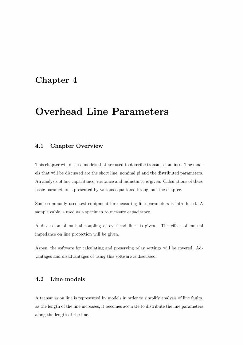
Grainger & Stevenson (1994) described a short line as 80 km long and it can reasonably
be represented by series resistance and inductance without loss of accuracy. The fact
that the shunt capacitance is very small in short lines, lumped parameters of inductance
and resistance are only considered in the line data.
VS is the sending end voltage, IS is the sending end current, R and L form the series
impedance. In figure 4.1, the sending end and the receiving end currents are exactly
the same so the voltage regulation of the circuit can be easily calculated. According to
(Grainger & Stevenson 1994), voltage regulation is given by:
Regulation =|VR,NL| − |VR,FL|
|VR,FL|pu (4.1)
Where
• |VR,NL| is the magnitude of the receiving end voltage at no load
• |VR,FL| is the magnitude of the receiving end voltage at full load
Figure 4.1: Short Line Model
Source: (Grainger & Stevenson 1994)
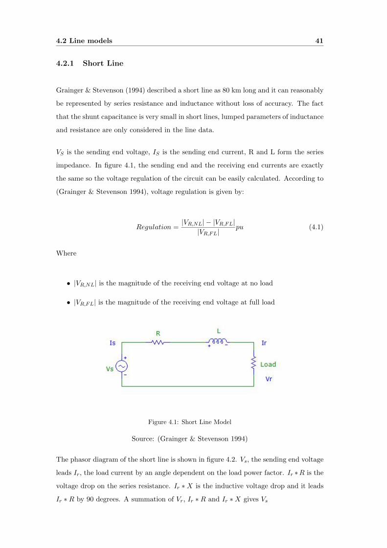
The phasor diagram of the short line is shown in figure 4.2. Vs, the sending end voltage
leads Ir, the load current by an angle dependent on the load power factor. Ir ∗R is the
voltage drop on the series resistance. Ir ∗X is the inductive voltage drop and it leads
Ir ∗R by 90 degrees. A summation of Vr, Ir ∗R and Ir ∗X gives Vs
4.2 Line models 42
Figure 4.2: Short Line Model
Source: (Grainger & Stevenson 1994)
4.2.2 Medium Length Line
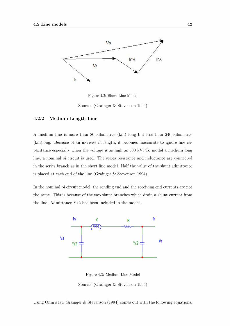
A medium line is more than 80 kilometres (km) long but less than 240 kilometres
(km)long. Because of an increase in length, it becomes inaccurate to ignore line ca-
pacitance especially when the voltage is as high as 500 kV. To model a medium long
line, a nominal pi circuit is used. The series resistance and inductance are connected
in the series branch as in the short line model. Half the value of the shunt admittance
is placed at each end of the line (Grainger & Stevenson 1994).
In the nominal pi circuit model, the sending end and the receiving end currents are not
the same. This is because of the two shunt branches which drain a shunt current from
the line. Admittance Y/2 has been included in the model.
Figure 4.3: Medium Line Model
Source: (Grainger & Stevenson 1994)
Using Ohm’s law Grainger & Stevenson (1994) comes out with the following equations:
4.2 Line models 43
Is = (Y
2Vs + Vr)
Y
2+ Ir (4.2)
Vs = (Y
2Vr + Ir)Z + Vr (4.3)
Vs = (Y Z
2+ 1)Vr + IrZ (4.4)
Thus
Is = (Y Z
4+ 1)Vr ∗ Y + Ir(
ZY
2+ 1) (4.5)
Let A = D but
A =Y Z
2+ 1 (4.6)
Let B = Z
C =Y Z
4+ 1 (4.7)
Thus
Vs = AVr +BIr (4.8)
Is = CVr +DIr (4.9)
A,B,C and D are constants of the transmission line and in most cases they are complex
numbers (Grainger & Stevenson 1994).
4.2.3 Long Line
A line is considered to be long if it is more than 240 km in length. The way to model
a long line is to use distributed parameters. This means that capacitance, inductance
and resistance values are distributed along the line as the length increases. This is a
more realistic approach because line parameters increase proportionally with the length
of the line.
Figure 4.4 shows the model of a long line where:
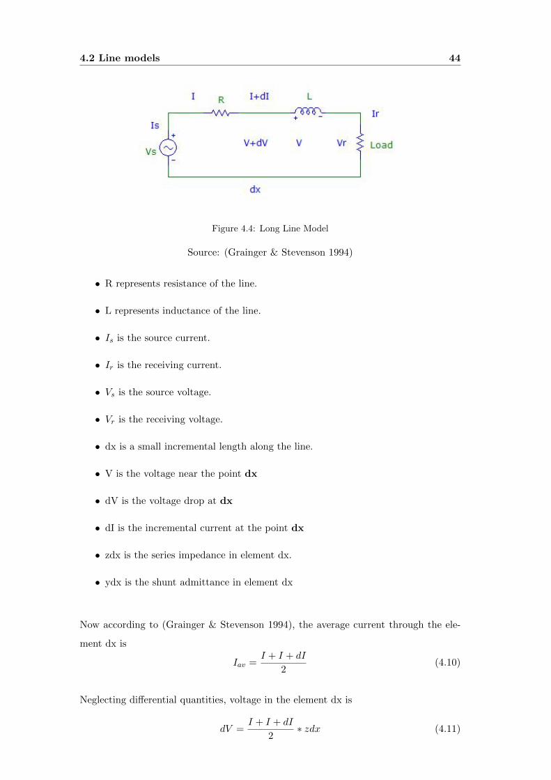
4.2 Line models 44
Figure 4.4: Long Line Model
Source: (Grainger & Stevenson 1994)
• R represents resistance of the line.
• L represents inductance of the line.
• Is is the source current.
• Ir is the receiving current.
• Vs is the source voltage.
• Vr is the receiving voltage.
• dx is a small incremental length along the line.
• V is the voltage near the point dx
• dV is the voltage drop at dx
• dI is the incremental current at the point dx
• zdx is the series impedance in element dx.
• ydx is the shunt admittance in element dx
Now according to (Grainger & Stevenson 1994), the average current through the ele-
ment dx is
Iav =I + I + dI
2(4.10)
Neglecting differential quantities, voltage in the element dx is
dV =I + I + dI
2∗ zdx (4.11)
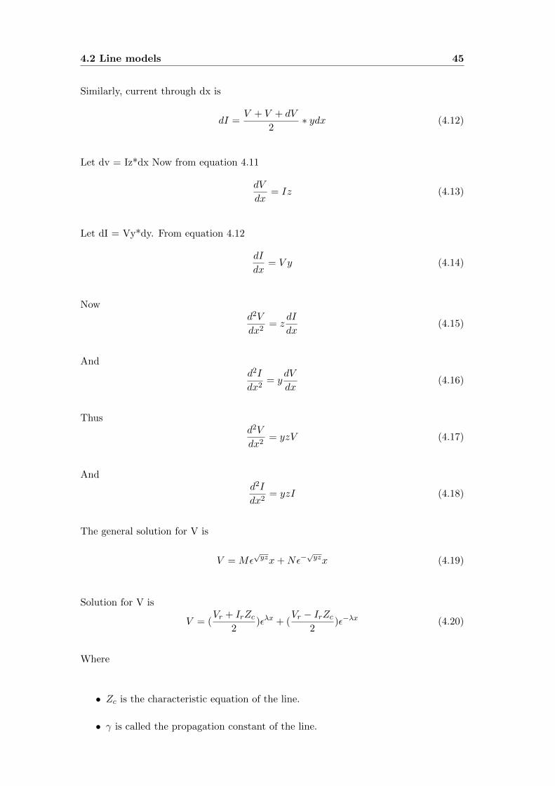
4.2 Line models 45
Similarly, current through dx is
dI =V + V + dV
2∗ ydx (4.12)
Let dv = Iz*dx Now from equation 4.11
dV
dx= Iz (4.13)
Let dI = Vy*dy. From equation 4.12
dI
dx= V y (4.14)
Nowd2V
dx2= z
dI
dx(4.15)
Andd2I
dx2= y
dV
dx(4.16)
Thusd2V
dx2= yzV (4.17)
Andd2I
dx2= yzI (4.18)
The general solution for V is
V = Mε√yzx+Nε−
√yzx (4.19)
Solution for V is
V = (Vr + IrZc
2)ελx + (
Vr − IrZc2
)ε−λx (4.20)
Where
• Zc is the characteristic equation of the line.
• γ is called the propagation constant of the line.
4.2 Line models 46
Zc =
√z
y(4.21)
γ =√zy (4.22)
Voltage V and current I can also be represented using hyperbolic functions when the
component ελx is replaced by hyperbolic functions.
sinhθ =εθ − ε−θ
2(4.23)
cosθ =εθ + ε−θ
2(4.24)
Hence
V = Vrcoshγx+ IrZcsinhγx (4.25)
And
I = Ircoshγx+VrZcsinhγx (4.26)
Equations 4.19 and 4.20 will give the rms values of voltage and current at any specified
point along the line in terms of distance x measured from the receiving end of the line
(Grainger & Stevenson 1994). This is possible if line parameters are known. The fact
that currents and voltages can be calculated at any point on the line, fault location
along the line can be done using a relay that can use equations 4.21 and 4.22 and log
the results in a memory location.
The GE L90 relay incorporates a fault recorder that keeps memory of the last 15
fault records (GE Multilin 2012). The date, time and cause of the fault is recorded.
The relay has the capability of measuring line currents and displaying the readings
front panel display of the relay. The relay also has capability to send measurements
information to a remote control centre.
The SEL 311L relay provides instantaneous metering, demand metering, maximum and
minimum metering and energy metering. The reported measurements include positive,
negative and zero sequence quantities for both local and remote ends of a line.
4.3 Determining Line Parameters 47
The Siemens 7SD5 relay has an inbuilt function for recording oscillographic fault
records. The measured quantities are sampled at intervals of 1 millisecond (mS) and
stored in a calculating buffer which operates at 20 samples per cycle (Siemens 2011).
When a fault occurs, the data is stored for an adjustable time up to a maximum total
of 5 seconds per fault. Thus a total of 8 faults can be saved in a time window spanning
15 seconds. The fault record memory is automatically updated by every new fault
entering the fault memory bank.
4.3 Determining Line Parameters
4.3.1 Calculation of Line Capacitance
Capacitance on a transmission line is caused by the potential difference between the
conductors. In power lines of 80 km and below, capacitive effect is low and can be
safely ignored. For lines longer than 80 km and at 500 kV, the effect of line capacitance
becomes increasingly important (Grainger & Stevenson 1994).
The electric flux density of a conductor placed in a uniform electric field is given by
Gauss’s law:
Df =q
2πx(4.27)
Where x is the distance in metres from the conductor to any radius x and q is the
instantaneous charge on the conductor in Coulombs.
The electric field strength of the conductor is given by:
E =q
2πkx(4.28)
The amount of work done in moving a unit charge from point D to D1, in an electric
field E is called the potential difference between D1 and D and is given by:
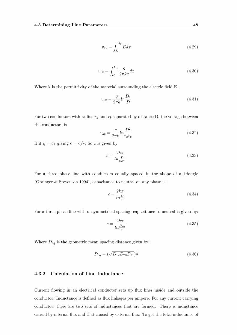
4.3 Determining Line Parameters 48
v12 =
∫ D1
DEdx (4.29)
v12 =
∫ D1
D
q
2πkxdx (4.30)
Where k is the permittivity of the material surrounding the electric field E.
v12 =q
2πklnD1
D(4.31)
For two conductors with radius ra and rb separated by distance D, the voltage between
the conductors is
vab =q
2πklnD2
rarb(4.32)
But q = cv giving c = q/v, So c is given by
c =2kπ
ln Drarb
(4.33)
For a three phase line with conductors equally spaced in the shape of a triangle
(Grainger & Stevenson 1994), capacitance to neutral on any phase is:
c =2kπ
lnDr(4.34)
For a three phase line with unsymmetrical spacing, capacitance to neutral is given by:
c =2kπ
lnDeq
r
(4.35)
Where Deq is the geometric mean spacing distance given by:
Deq = (√D12D23D31)
13 (4.36)
4.3.2 Calculation of Line Inductance
Current flowing in an electrical conductor sets up flux lines inside and outside the
conductor. Inductance is defined as flux linkages per ampere. For any current carrying
conductor, there are two sets of inductances that are formed. There is inductance
caused by internal flux and that caused by external flux. To get the total inductance of
4.3 Determining Line Parameters 49
the conductor, inductance due to internal flux and inductance due to external flux have
to be computed. Figure 4.5 shows a cross section of a conductor carrying a current I.
The magnetomotive force on the line is given by Ampere’s law:
Figure 4.5: Cross section of a cylindrical conductor
Source: (Grainger & Stevenson 1994)
Where
• H is the magnetic field strength.
• I is the enclosed current in the conductor
• ds is the distance along the path which is at a distance x metres from the centre
of the conductor.
mmf =
∮H.ds (4.37)
Because ampere turns are measured in amps, the result of solving equation 4.37 gives a
current. This current is an enclosed current as indicated on the integral symbol. Thus;
Ix =
∮H.ds (4.38)
A circle of radius x metres has a circumference:
cir = 2πx (4.39)
4.3 Determining Line Parameters 50
So equation 4.38 becomes
Ix = 2πxH (4.40)
Now considering a uniform current density, a ratio of areas can be considered (Grainger
& Stevenson 1994). Current I is flowing in the whole conductor. Hence
Ix =x2π
r2πI (4.41)
Using equations 4.40 and 4.41, Hx the magnetic field strength at radius x is:
Hx =x
2πr2I (4.42)
From Bx = µHx
Bx =xµ
2πr2I (4.43)
The ratio of areas is x2/r2 So total flux is Bx times ratio of areas
φ =x3µ
2πr4I (4.44)
Therefore internal flux linkage λ is:
λint =
∫ r
0
x3µ
2πr4Idx (4.45)
λint =µ
8πI (4.46)
Inductance is flux linkage divided by the current, so:
Lint =µ
8π(H/m) (4.47)
External Flux Considering any two points M and N at distances D and d metres
respectively from the centre of a current carrying conductor, the external flux will be
concentric to both points. For a flux line at a distance x metres from the centre of the
conductor, the current is given by:
I = 2πxHx (4.48)
4.3 Determining Line Parameters 51
Using B = µHx, Bx is:
Bx =Iµ
2πx(4.49)
λext =
∫ D
d
Iµ
2πxdx (4.50)
λext =Iµ
2πlnD
d(4.51)
External Inductance is
λext =µ
2πlnD
d(4.52)
Therefore the total inductance of the conductor is (Grainger & Stevenson 1994):
λtot =µ
8π+Iµ
2πlnD
d(H/m) (4.53)
For air µ is 4π10−7 H/m.
Inductance per phase in three phase lines with equilateral spacing is:
L = 2 ∗ 10−7lnD
DsH/m (4.54)
Where Ds is the geometric mean ratio as shown in equation 4.36.
For For bundled conductors as in most cases on 500 kV lines, the inductance is given
by;
4.3.3 Obtaining Line Parameters by Measurements
Line capacitance, inductance and resistance can be found by carrying out measure-
ments. The study below shows line parameters that were obtained on a 500 kV line
by direct measurements. The 500 kV Transmission line was built in the year 2000
in China. It is 83 km long and it links two 500 kV substations namely Changping
and Fangshan (Wang & etal 2000). The 500 kV line carries 1340 MW (Megawatts) of
electric power. The results of tests carried out are shown in table 4.1.
The 500 kV line has 6 conductors per phase and all the phases are in a straight horizon-
tal line. When commissioning the 500 kV line, they did a switching surge over voltage
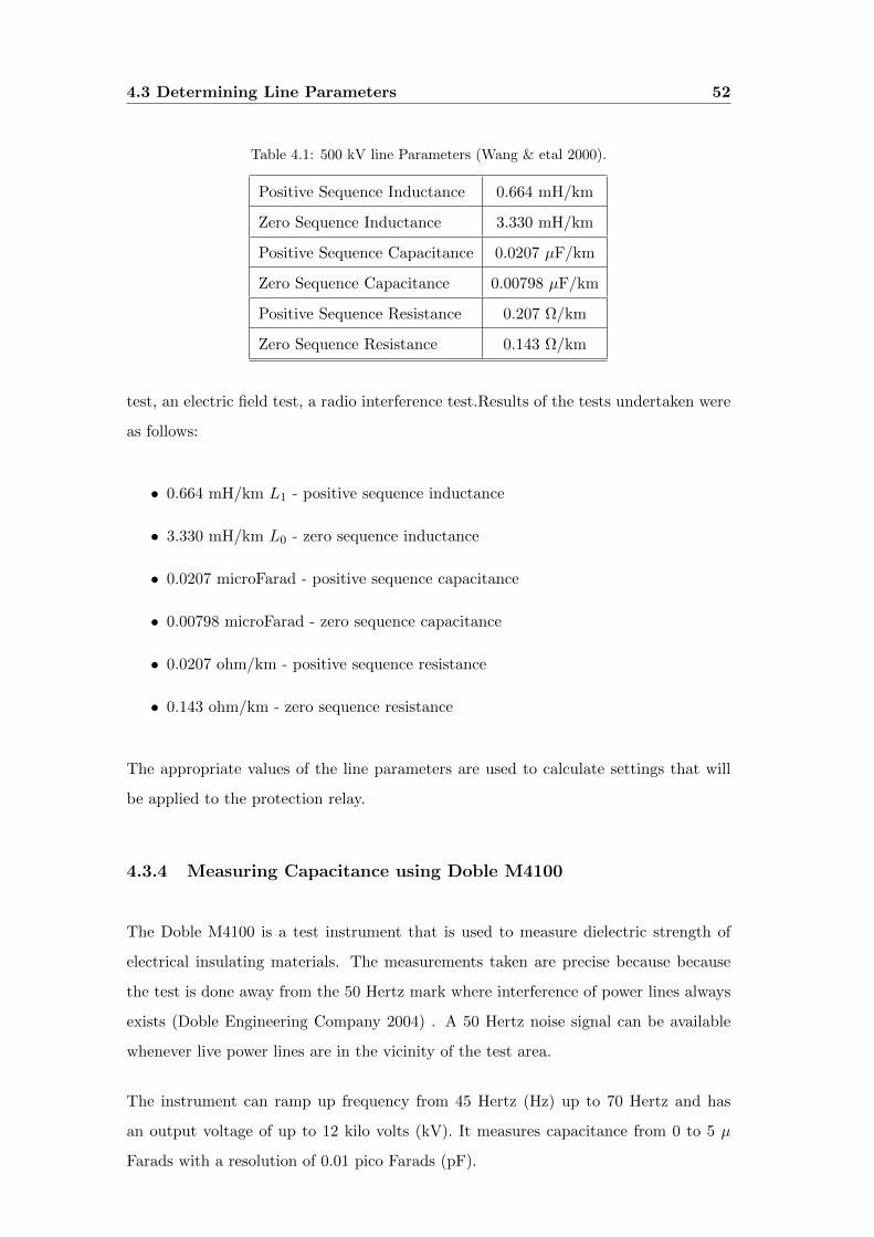
4.3 Determining Line Parameters 52
Table 4.1: 500 kV line Parameters (Wang & etal 2000).
Positive Sequence Inductance 0.664 mH/km
Zero Sequence Inductance 3.330 mH/km
Positive Sequence Capacitance 0.0207 µF/km
Zero Sequence Capacitance 0.00798 µF/km
Positive Sequence Resistance 0.207 Ω/km
Zero Sequence Resistance 0.143 Ω/km
test, an electric field test, a radio interference test.Results of the tests undertaken were
as follows:
• 0.664 mH/km L1 - positive sequence inductance
• 3.330 mH/km L0 - zero sequence inductance
• 0.0207 microFarad - positive sequence capacitance
• 0.00798 microFarad - zero sequence capacitance
• 0.0207 ohm/km - positive sequence resistance
• 0.143 ohm/km - zero sequence resistance
The appropriate values of the line parameters are used to calculate settings that will
be applied to the protection relay.
4.3.4 Measuring Capacitance using Doble M4100
The Doble M4100 is a test instrument that is used to measure dielectric strength of
electrical insulating materials. The measurements taken are precise because because
the test is done away from the 50 Hertz mark where interference of power lines always
exists (Doble Engineering Company 2004) . A 50 Hertz noise signal can be available
whenever live power lines are in the vicinity of the test area.
The instrument can ramp up frequency from 45 Hertz (Hz) up to 70 Hertz and has
an output voltage of up to 12 kilo volts (kV). It measures capacitance from 0 to 5 µ
Farads with a resolution of 0.01 pico Farads (pF).
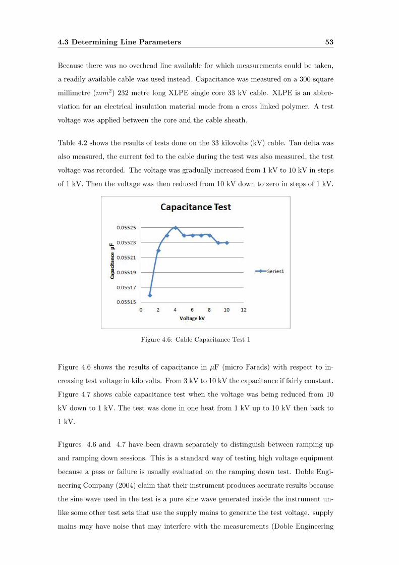
4.3 Determining Line Parameters 53
Because there was no overhead line available for which measurements could be taken,
a readily available cable was used instead. Capacitance was measured on a 300 square
millimetre (mm2) 232 metre long XLPE single core 33 kV cable. XLPE is an abbre-
viation for an electrical insulation material made from a cross linked polymer. A test
voltage was applied between the core and the cable sheath.
Table 4.2 shows the results of tests done on the 33 kilovolts (kV) cable. Tan delta was
also measured, the current fed to the cable during the test was also measured, the test
voltage was recorded. The voltage was gradually increased from 1 kV to 10 kV in steps
of 1 kV. Then the voltage was then reduced from 10 kV down to zero in steps of 1 kV.
Figure 4.6: Cable Capacitance Test 1
Figure 4.6 shows the results of capacitance in µF (micro Farads) with respect to in-
creasing test voltage in kilo volts. From 3 kV to 10 kV the capacitance if fairly constant.
Figure 4.7 shows cable capacitance test when the voltage was being reduced from 10
kV down to 1 kV. The test was done in one heat from 1 kV up to 10 kV then back to
1 kV.
Figures 4.6 and 4.7 have been drawn separately to distinguish between ramping up
and ramping down sessions. This is a standard way of testing high voltage equipment
because a pass or failure is usually evaluated on the ramping down test. Doble Engi-
neering Company (2004) claim that their instrument produces accurate results because
the sine wave used in the test is a pure sine wave generated inside the instrument un-
like some other test sets that use the supply mains to generate the test voltage. supply
mains may have noise that may interfere with the measurements (Doble Engineering
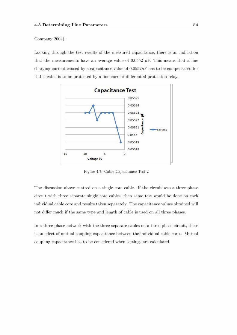
4.3 Determining Line Parameters 54
Company 2004).
Looking through the test results of the measured capacitance, there is an indication
that the measurements have an average value of 0.0552 µF. This means that a line
charging current caused by a capacitance value of 0.0552µF has to be compensated for
if this cable is to be protected by a line current differential protection relay.
Figure 4.7: Cable Capacitance Test 2
The discussion above centred on a single core cable. If the circuit was a three phase
circuit with three separate single core cables, then same test would be done on each
individual cable core and results taken separately. The capacitance values obtained will
not differ much if the same type and length of cable is used on all three phases.
In a three phase network with the three separate cables on a three phase circuit, there
is an effect of mutual coupling capacitance between the individual cable cores. Mutual
coupling capacitance has to be considered when settings are calculated.

4.3 Determining Line Parameters 55
Table 4.2: Measuring Capacitance of a 33 kV Cable
Voltage kV Current mA Tan Delta Capacitance µF
1 17.323 0.021 0.05516
2 34.701 0.019 0.05522
3 52.063 0.016 0.05524
4 69.416 0.016 0.05525
5 86.775 0.016 0.05524
6 104.12 0.020 0.05524
7 121.472 0.021 0.05524
8 138.838 0.027 0.05524
9 156.174 0.027 0.05523
10 173.535 0.029 0.05523
9 156.74 0.027 0.0523
8 138.810 0.026 0.05524
7 121.449 0.019 0.05522
6 104.109 0.019 0.05523
5 86.755 0.014 0.05523
4 69.411 0.014 0.05523
3 52.059 0.014 0.05523
2 34.692 0.017 0.05521
1 17.339 0.019 0.05519
4.3.5 Line Impedance using Omicron CP CU1
There is an Omicron test set that measures line impedance. It is the Omicron CP
CU1. This test instrument is used in conjunction with Omicron CPC 100. Because of
the possibility of encountering life threatening voltages of 600 v (volts) during a test,
it is strongly recommended to keep safe from the test unit’s CP GB1 grounding box
(Omicron Electronics 2010).
The CP GB1 is a surge arrestor which shorts line terminals to ground when a high
voltage appears for a long time. If the high voltage appears for a short time, an arc
discharges the voltage to ground without destroying the CP GB1 unit. The CP CU1
unit measures impedance by applying an ac voltage to the test item, voltage and current
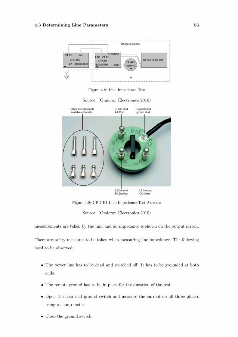
4.3 Determining Line Parameters 56
Figure 4.8: Line Impedance Test
Source: (Omicron Electronics 2010)
Figure 4.9: CP GB1 Line Impedance Test Arrestor
Source: (Omicron Electronics 2010)
measurements are taken by the unit and an impedance is shown on the output screen.
There are safety measures to be taken when measuring line impedance. The following
need to be observed;
• The power line has to be dead and switched off. It has to be grounded at both
ends.
• The remote ground has to be in place for the duration of the test.
• Open the near end ground switch and measure the current on all three phases
using a clamp meter.
• Close the ground switch.
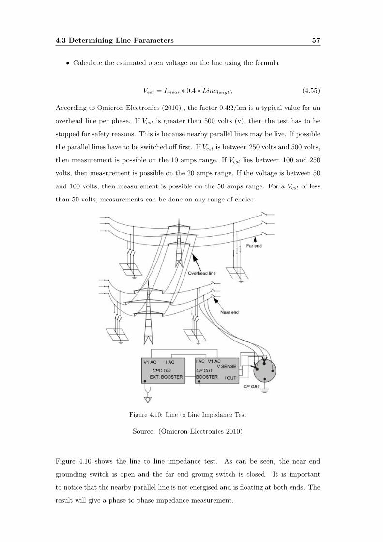
4.3 Determining Line Parameters 57
• Calculate the estimated open voltage on the line using the formula
Vest = Imeas ∗ 0.4 ∗ Linelength (4.55)
According to Omicron Electronics (2010) , the factor 0.4Ω/km is a typical value for an
overhead line per phase. If Vest is greater than 500 volts (v), then the test has to be
stopped for safety reasons. This is because nearby parallel lines may be live. If possible
the parallel lines have to be switched off first. If Vest is between 250 volts and 500 volts,
then measurement is possible on the 10 amps range. If Vest lies between 100 and 250
volts, then measurement is possible on the 20 amps range. If the voltage is between 50
and 100 volts, then measurement is possible on the 50 amps range. For a Vest of less
than 50 volts, measurements can be done on any range of choice.
Figure 4.10: Line to Line Impedance Test
Source: (Omicron Electronics 2010)
Figure 4.10 shows the line to line impedance test. As can be seen, the near end
grounding switch is open and the far end groung switch is closed. It is important
to notice that the nearby parallel line is not energised and is floating at both ends. The
result will give a phase to phase impedance measurement.
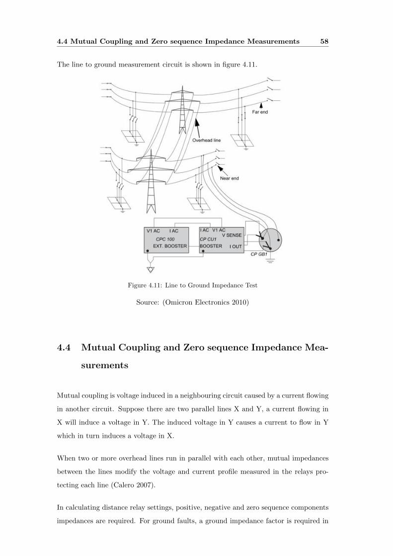
4.4 Mutual Coupling and Zero sequence Impedance Measurements 58
The line to ground measurement circuit is shown in figure 4.11.
Figure 4.11: Line to Ground Impedance Test
Source: (Omicron Electronics 2010)
4.4 Mutual Coupling and Zero sequence Impedance Mea-
surements
Mutual coupling is voltage induced in a neighbouring circuit caused by a current flowing
in another circuit. Suppose there are two parallel lines X and Y, a current flowing in
X will induce a voltage in Y. The induced voltage in Y causes a current to flow in Y
which in turn induces a voltage in X.
When two or more overhead lines run in parallel with each other, mutual impedances
between the lines modify the voltage and current profile measured in the relays pro-
tecting each line (Calero 2007).
In calculating distance relay settings, positive, negative and zero sequence components
impedances are required. For ground faults, a ground impedance factor is required in
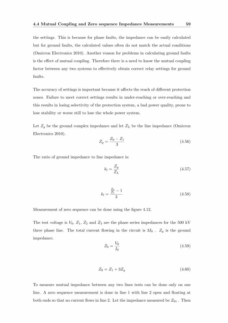
4.4 Mutual Coupling and Zero sequence Impedance Measurements 59
the settings. This is because for phase faults, the impedance can be easily calculated
but for ground faults, the calculated values often do not match the actual conditions
(Omicron Electronics 2010). Another reason for problems in calculating ground faults
is the effect of mutual coupling. Therefore there is a need to know the mutual coupling
factor between any two systems to effectively obtain correct relay settings for ground
faults.
The accuracy of settings is important because it affects the reach of different protection
zones. Failure to meet correct settings results in under-reaching or over-reaching and
this results in losing selectivity of the protection system, a bad power quality, prone to
lose stability or worse still to lose the whole power system.
Let Zg be the ground complex impedance and let ZL be the line impedance (Omicron
Electronics 2010).
Zg =Z0 − Z1
3(4.56)
The ratio of ground impedance to line impedance is:
kl =ZgZL
(4.57)
kl =Z0Z1− 1
3(4.58)
Measurement of zero sequence can be done using the figure 4.12.
The test voltage is V0, Z1, Z2 and Z3 are the phase series impedances for the 500 kV
three phase line. The total current flowing in the circuit is 3I0 . Zg is the ground
impedance.
Z0 =V0I0
(4.59)
Z0 = Z1 + 3Zg (4.60)
To measure mutual impedance between any two lines tests can be done only on one
line. A zero sequence measurement is done in line 1 with line 2 open and floating at
both ends so that no current flows in line 2. Let the impedance measured be Z01 . Then
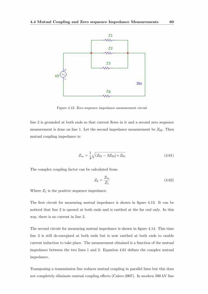
4.4 Mutual Coupling and Zero sequence Impedance Measurements 60
Figure 4.12: Zero sequence impedance measurement circuit
line 2 is grounded at both ends so that current flows in it and a second zero sequence
measurement is done on line 1. Let the second impedance measurement be Z02. Then
mutual coupling impedance is:
Zm =1
3
√(Z01 − 3Z02) ∗ Z01 (4.61)
The complex coupling factor can be calculated from:
Zk =ZmZ1
(4.62)
Where Z1 is the positive sequence impedance.
The first circuit for measuring mutual impedance is shown in figure 4.13. It can be
noticed that line 2 is opened at both ends and is earthed at the far end only. In this
way, there is no current in line 2.
The second circuit for measuring mutual impedance is shown in figure 4.14. This time
line 2 is still de-energised at both ends but is now earthed at both ends to enable
current induction to take place. The measurement obtained is a function of the mutual
impedance between the two lines 1 and 2. Equation 4.61 defines the complex mutual
impedance.
Transposing a transmission line reduces mutual coupling in parallel lines but this does
not completely eliminate mutual coupling effects (Calero 2007). In modern 500 kV line
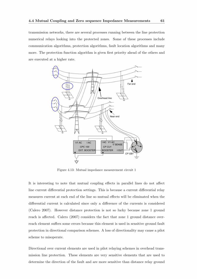
4.4 Mutual Coupling and Zero sequence Impedance Measurements 61
transmission networks, there are several processes running between the line protection
numerical relays looking into the protected zones. Some of these processes include
communication algorithms, protection algorithms, fault location algorithms and many
more. The protection function algorithm is given first priority ahead of the others and
are executed at a higher rate.
Figure 4.13: Mutual impedance measurement circuit 1
It is interesting to note that mutual coupling effects in parallel lines do not affect
line current differential protection settings. This is because a current differential relay
measures current at each end of the line so mutual effects will be eliminated when the
differential current is calculated since only a difference of the currents is considered
(Calero 2007). However distance protection is not so lucky because zone 1 ground
reach is affected. Calero (2007) considers the fact that zone 1 ground distance over-
reach element suffers some errors because this element is used in sensitive ground fault
protection in directional comparison schemes. A loss of directionality may cause a pilot
scheme to misoperate.
Directional over current elements are used in pilot relaying schemes in overhead trans-
mission line protection. These elements are very sensitive elements that are used to
determine the direction of the fault and are more sensitive than distance relay ground
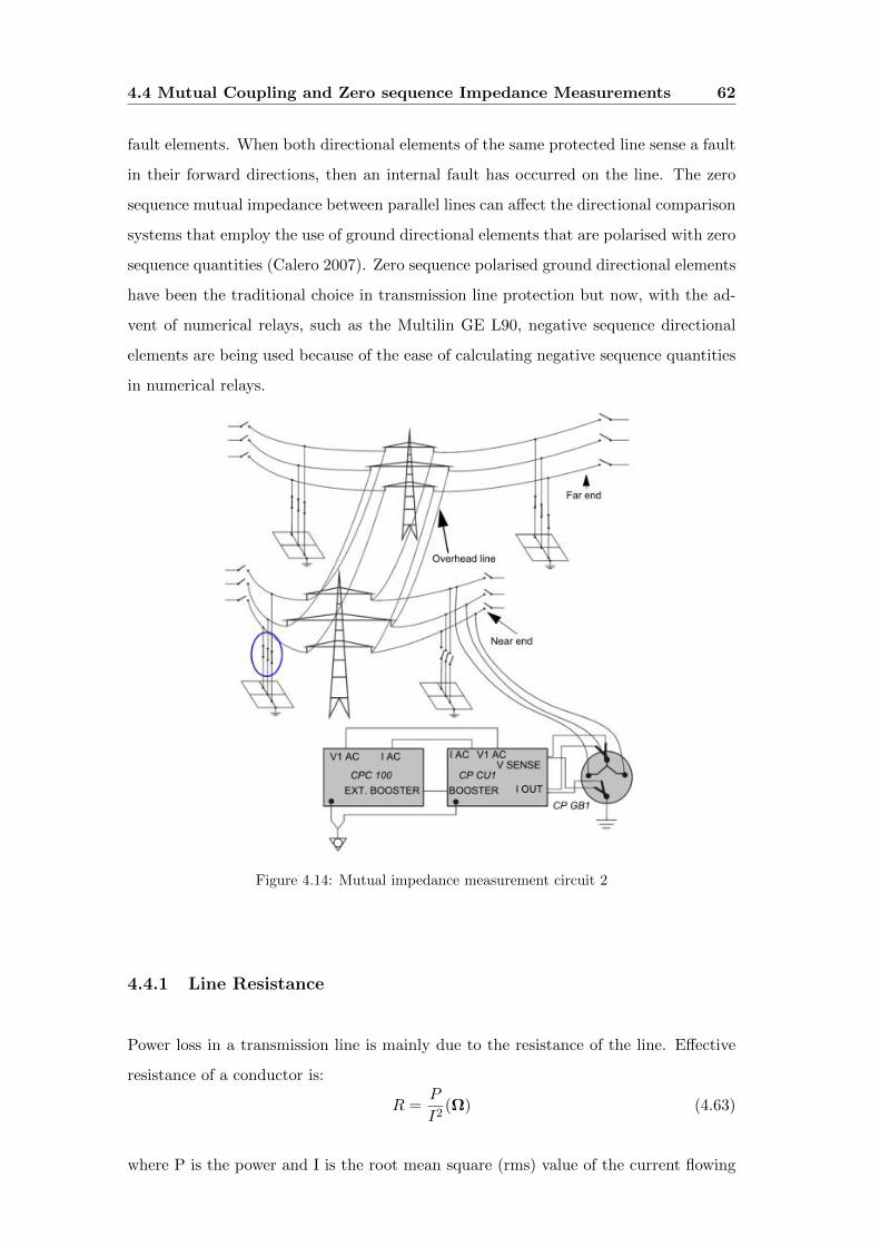
4.4 Mutual Coupling and Zero sequence Impedance Measurements 62
fault elements. When both directional elements of the same protected line sense a fault
in their forward directions, then an internal fault has occurred on the line. The zero
sequence mutual impedance between parallel lines can affect the directional comparison
systems that employ the use of ground directional elements that are polarised with zero
sequence quantities (Calero 2007). Zero sequence polarised ground directional elements
have been the traditional choice in transmission line protection but now, with the ad-
vent of numerical relays, such as the Multilin GE L90, negative sequence directional
elements are being used because of the ease of calculating negative sequence quantities
in numerical relays.
Figure 4.14: Mutual impedance measurement circuit 2
4.4.1 Line Resistance
Power loss in a transmission line is mainly due to the resistance of the line. Effective
resistance of a conductor is:
R =P
I2(Ω) (4.63)
where P is the power and I is the root mean square (rms) value of the current flowing
4.4 Mutual Coupling and Zero sequence Impedance Measurements 63
in the conductor. Effective resistance can only be equal to the direct current (dc)
resistance if the current is uniformly distributed in the conductor (Grainger & Stevenson
1994).
Resistance is given by
R =ρl
A(Ω) (4.64)
Where:
• A is the cross sectional area
• l is the length
• ρ is the resistivity of the conductor
The resistance in stranded conductors tends to be higher than that described by equa-
tion 4.64 because the spiralling of the stands makes them longer than the conductor
itself. Resistance of metallic conductors varies in a linear fashion with temperature
over the normal operating range (Grainger & Stevenson 1994).
The resistance of a conductor varies in value according to:
R2
R1=T + t2T + t1
(4.65)
Where T is a temperature that depends on the material type. R1 and R2 being the
temperatures at t1 and t2.
Only direct current (DC) flows uniformly across the cross sectional area of a conductor.
An increase in frequency of the current causes the current to be distributed in a non
uniform manner across the area of the conductor. This effect is called skin effect. In
circular conductors, the current density increases from the centre to the surface.
4.4.2 Line Parameters Using ASPEN software
Another way of determining line parameters is to use a software called Aspen. The
Aspen software programme has an area specifically dedicated to overhead lines. It
calculates electrical parameters of overhead lines including underground cables. The

4.4 Mutual Coupling and Zero sequence Impedance Measurements 64
software incorporates a graphical interface that shows layout of circuits of overhead
lines and also includes the physical construction of cables (Aspen 2013).
The software covers work on:
• Tests on transposed and untransposed circuits.
• Tests on bundled conductors.
• One or more ground wires, segmented or unsegmented.
• Any number of line sections transposed or untransposed.
• Single, two or three circuits in the same easement.
• Branch impedance and admittance matrices in the phase domain are calculated.
• Cable sheaths, that are single point bonded, solidly bonded or cross bonded are
evaluated.
• Nodal capacitance and susceptance matrices in the phase domain are calculated.
• Positive and zero sequence self impedance and capacitance are calculated.
The Aspen software has a lines database. In this one any line related information is
stored including data on line parameter calculations. The database allows the user
to maintain a library of overhead towers, wires and cables so that any model can be
created. The Aspen line constants programme is a 32 bit programme that runs on
Windows Vista, XP, Windows 7 and 8 (Aspen 2013).
4.5 Chapter Summary 65
4.5 Chapter Summary
This chapter has covered three parameters of a transmission line. Line capacitance,
inductance and resistance have been shown to increase with length of the line.
For a current carrying conductor, there is internal and external inductance. Total
inductance is the sum of the two inductances. The inductance of an overhead line
depends on the permeability of air.
Capacitance depends on the spacing distance between any two conductors. Line ca-
pacitance depends on the level of the voltage on the line.
Resistance of a conductor depends on the resistivity of the conductor material. Resis-
tance in metallic conductors increases with temperature but is generally linear over the
normal operating temperatures.
Besides calculations, line parameters can be measured directly. A doble M4000 test set
has been described and it measures electrical insulation of materials. A demonstration
of measurement of capacitance using this instrument has been shown on figures 4.6 and
4.7 where capacitance of a 33 kV cable has been measured.
The Omicron CPU1 instrument has been discussed and also measures line impedance
including mutual impedance. Zero sequence measurements can also be done with this
instrument.
Mutual impedance has been introduced and it has been found to affect distance pro-
tection relay ground settings. Careful consideration of mutual impedance in parallel
line is critical in the correct operation of distance protection.
The Aspen software is a tool where line parameters can be calculated and stored. Relay
settings and protection maintenance schedules can be planned using the Aspen software
package.
Chapter 5
Effect of Line capacitance on
Protection Settings
5.1 Chapter Overview
This chapter deals with how line capacitance affects pilot wire protection. The effect
of line capacitance on line current differential protection is discussed. Phasor diagrams
are used to show the capacitive current and load currents.
Various equations will be used to describe the line without capacitance and then with
capacitance in place. Firstly effects on line current differential will be covered then at
the end effects on distance protection will be discussed.
Further effects on capacitance variation will be shown in chapter 9 where simulations
of phase to phase, phase to ground and three phase faults are simulated using Matlab
and Simulink software.
5.2 Line Capacitance and Pilot wire Protection Protec-
tion
Considering the pilot wire scheme that was discussed in chapter 2, the pilot wires play
a very important part in maintaining communication between both ends of a protected
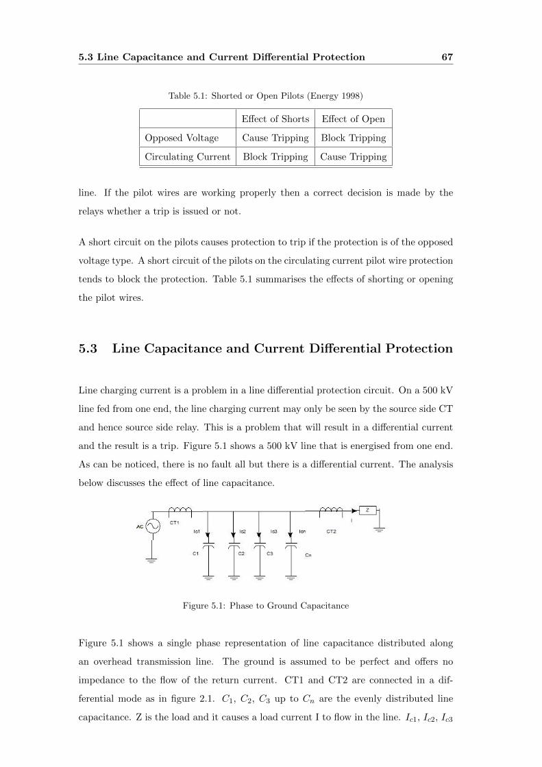
5.3 Line Capacitance and Current Differential Protection 67
Table 5.1: Shorted or Open Pilots (Energy 1998)
Effect of Shorts Effect of Open
Opposed Voltage Cause Tripping Block Tripping
Circulating Current Block Tripping Cause Tripping
line. If the pilot wires are working properly then a correct decision is made by the
relays whether a trip is issued or not.
A short circuit on the pilots causes protection to trip if the protection is of the opposed
voltage type. A short circuit of the pilots on the circulating current pilot wire protection
tends to block the protection. Table 5.1 summarises the effects of shorting or opening
the pilot wires.
5.3 Line Capacitance and Current Differential Protection
Line charging current is a problem in a line differential protection circuit. On a 500 kV
line fed from one end, the line charging current may only be seen by the source side CT
and hence source side relay. This is a problem that will result in a differential current
and the result is a trip. Figure 5.1 shows a 500 kV line that is energised from one end.
As can be noticed, there is no fault all but there is a differential current. The analysis
below discusses the effect of line capacitance.
Figure 5.1: Phase to Ground Capacitance
Figure 5.1 shows a single phase representation of line capacitance distributed along
an overhead transmission line. The ground is assumed to be perfect and offers no
impedance to the flow of the return current. CT1 and CT2 are connected in a dif-
ferential mode as in figure 2.1. C1, C2, C3 up to Cn are the evenly distributed line
capacitance. Z is the load and it causes a load current I to flow in the line. Ic1, Ic2, Ic3
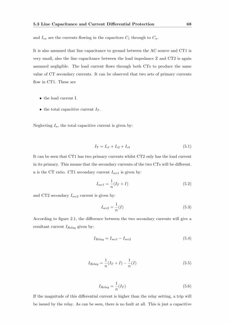
5.3 Line Capacitance and Current Differential Protection 68
and Icn are the currents flowing in the capacitors C1 through to Cn.
It is also assumed that line capacitance to ground between the AC source and CT1 is
very small, also the line capacitance between the load impedance Z and CT2 is again
assumed negligible. The load current flows through both CTs to produce the same
value of CT secondary currents. It can be observed that two sets of primary currents
flow in CT1. These are
• the load current I.
• the total capacitive current IT .
Neglecting In, the total capacitive current is given by:
IT = Ic1 + Ic2 + Ic3 (5.1)
It can be seen that CT1 has two primary currents whilst CT2 only has the load current
in its primary. This means that the secondary currents of the two CTs will be different.
n is the CT ratio. CT1 secondary current Isec1 is given by:
Isec1 =1
n(IT + I) (5.2)
and CT2 secondary Isec2 current is given by:
Isec2 =1
n(I) (5.3)
According to figure 2.1, the difference between the two secondary currents will give a
resultant current IRelay given by:
IRelay = Isec1 − Isec2 (5.4)
IRelay =1
n(IT + I)− 1
n(I) (5.5)
IRelay =1
n(IT ) (5.6)
If the magnitude of this differential current is higher than the relay setting, a trip will
be issued by the relay. As can be seen, there is no fault at all. This is just a capacitive
5.3 Line Capacitance and Current Differential Protection 69
current generated by the shunt capacitances which are distributed along the over head
line (500 kV) in this case. Somehow there must be a way to suppress this false tripping
current. Numeric relays have a setting where line charging current is blocked from
causing a trip. This feature and its associated settings will be discussed in chapter 6.
From table ??, the positive sequence capacitance for the 500 kV line for this project is
0.0207 µF (Wang & etal 2000).
From the well known capacitor current equation:
IC = 2 ∗ π ∗ f ∗ C ∗ V (5.7)
Where IC is the positive sequence line charging current, V is the phase to ground
voltage and f is the supply frequency. A detailed calculation will be done in chapter 7.
Figure 5.2 shows the phasor diagram of currents in CT1. The phase to ground voltage
is represented by vector OA and this is the reference phasor.
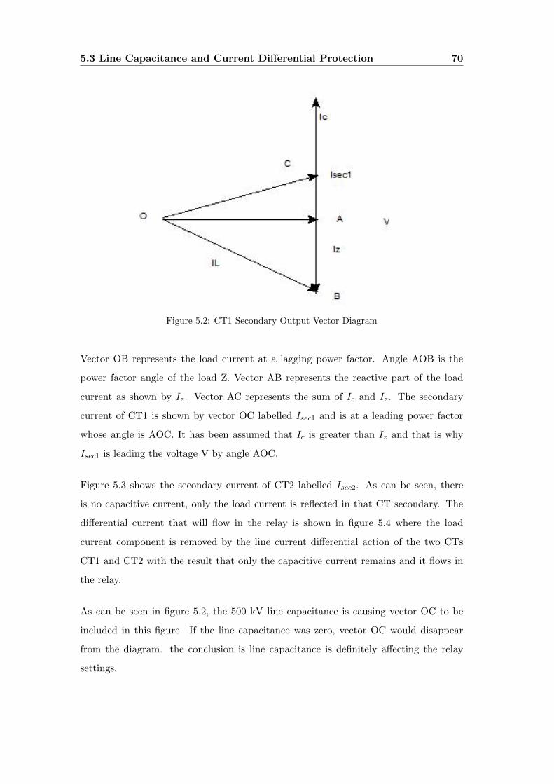
5.3 Line Capacitance and Current Differential Protection 70
Figure 5.2: CT1 Secondary Output Vector Diagram
Vector OB represents the load current at a lagging power factor. Angle AOB is the
power factor angle of the load Z. Vector AB represents the reactive part of the load
current as shown by Iz. Vector AC represents the sum of Ic and Iz. The secondary
current of CT1 is shown by vector OC labelled Isec1 and is at a leading power factor
whose angle is AOC. It has been assumed that Ic is greater than Iz and that is why
Isec1 is leading the voltage V by angle AOC.
Figure 5.3 shows the secondary current of CT2 labelled Isec2. As can be seen, there
is no capacitive current, only the load current is reflected in that CT secondary. The
differential current that will flow in the relay is shown in figure 5.4 where the load
current component is removed by the line current differential action of the two CTs
CT1 and CT2 with the result that only the capacitive current remains and it flows in
the relay.
As can be seen in figure 5.2, the 500 kV line capacitance is causing vector OC to be
included in this figure. If the line capacitance was zero, vector OC would disappear
from the diagram. the conclusion is line capacitance is definitely affecting the relay
settings.
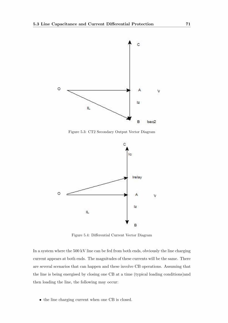
5.3 Line Capacitance and Current Differential Protection 71
Figure 5.3: CT2 Secondary Output Vector Diagram
Figure 5.4: Differential Current Vector Diagram
In a system where the 500 kV line can be fed from both ends, obviously the line charging
current appears at both ends. The magnitudes of these currents will be the same. There
are several scenarios that can happen and these involve CB operations. Assuming that
the line is being energised by closing one CB at a time (typical loading conditions)and
then loading the line, the following may occur:
• the line charging current when one CB is closed.
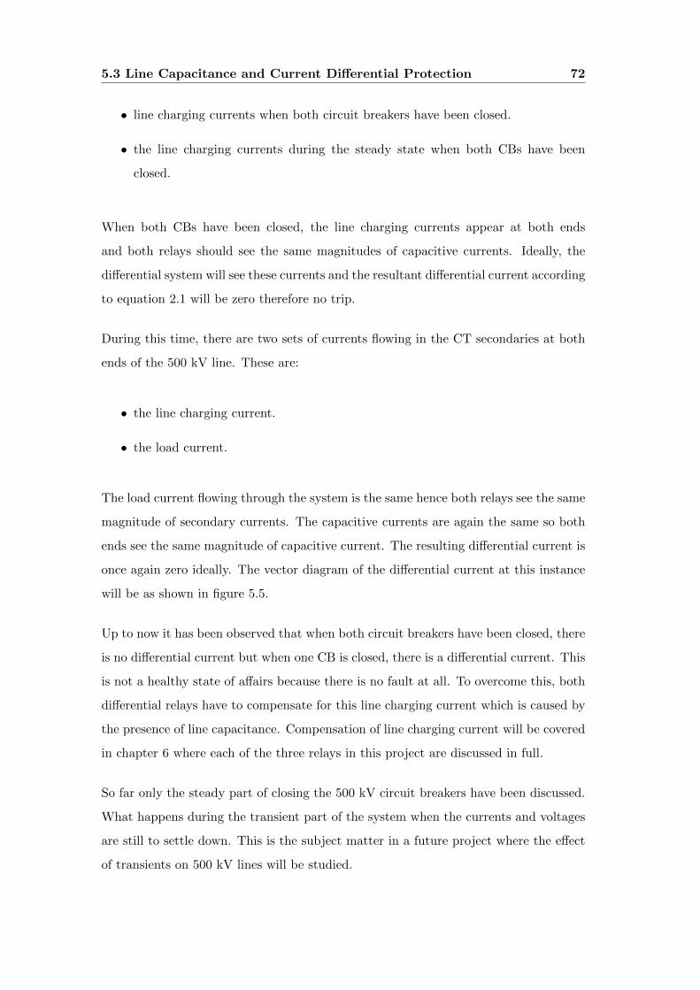
5.3 Line Capacitance and Current Differential Protection 72
• line charging currents when both circuit breakers have been closed.
• the line charging currents during the steady state when both CBs have been
closed.
When both CBs have been closed, the line charging currents appear at both ends
and both relays should see the same magnitudes of capacitive currents. Ideally, the
differential system will see these currents and the resultant differential current according
to equation 2.1 will be zero therefore no trip.
During this time, there are two sets of currents flowing in the CT secondaries at both
ends of the 500 kV line. These are:
• the line charging current.
• the load current.
The load current flowing through the system is the same hence both relays see the same
magnitude of secondary currents. The capacitive currents are again the same so both
ends see the same magnitude of capacitive current. The resulting differential current is
once again zero ideally. The vector diagram of the differential current at this instance
will be as shown in figure 5.5.
Up to now it has been observed that when both circuit breakers have been closed, there
is no differential current but when one CB is closed, there is a differential current. This
is not a healthy state of affairs because there is no fault at all. To overcome this, both
differential relays have to compensate for this line charging current which is caused by
the presence of line capacitance. Compensation of line charging current will be covered
in chapter 6 where each of the three relays in this project are discussed in full.
So far only the steady part of closing the 500 kV circuit breakers have been discussed.
What happens during the transient part of the system when the currents and voltages
are still to settle down. This is the subject matter in a future project where the effect
of transients on 500 kV lines will be studied.
5.4 Line Capacitance and Distance Protection 73
Figure 5.5: Relay Differential Current Vector Diagram
5.4 Line Capacitance and Distance Protection
Distance protection is not immune to the effects of line capacitance. Because distance
protection measures the impedance of a line, the line capacitance alters the impedance
seen by the relay as seen from the relaying point. The general equation of symmetrical
components is shown in equation 5.8I+
I−
I0
=1
3
1 a a2
1 a2 a
1 1 1
IA
IB
IC
(5.8)
Using the method of symmetrical components as shown in equation 5.8, an A phase
to ground fault can be analysed. In an A phase to ground fault,
IBf = ICf = 0 (5.9)
Hence
I+ =1
3∗ IAf (5.10)
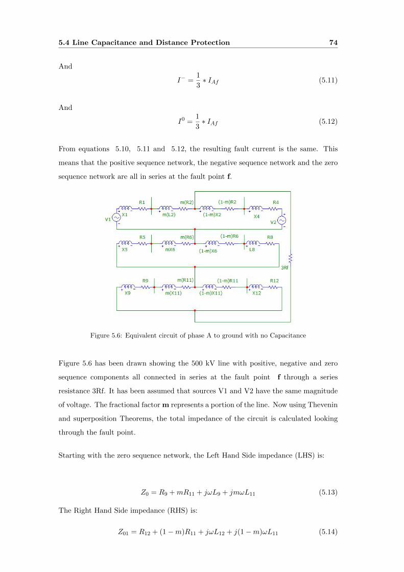
5.4 Line Capacitance and Distance Protection 74
And
I− =1
3∗ IAf (5.11)
And
I0 =1
3∗ IAf (5.12)
From equations 5.10, 5.11 and 5.12, the resulting fault current is the same. This
means that the positive sequence network, the negative sequence network and the zero
sequence network are all in series at the fault point f.
Figure 5.6: Equivalent circuit of phase A to ground with no Capacitance
Figure 5.6 has been drawn showing the 500 kV line with positive, negative and zero
sequence components all connected in series at the fault point f through a series
resistance 3Rf. It has been assumed that sources V1 and V2 have the same magnitude
of voltage. The fractional factor m represents a portion of the line. Now using Thevenin
and superposition Theorems, the total impedance of the circuit is calculated looking
through the fault point.
Starting with the zero sequence network, the Left Hand Side impedance (LHS) is:
Z0 = R9 +mR11 + jωL9 + jmωL11 (5.13)
The Right Hand Side impedance (RHS) is:
Z01 = R12 + (1−m)R11 + jωL12 + j(1−m)ωL11 (5.14)
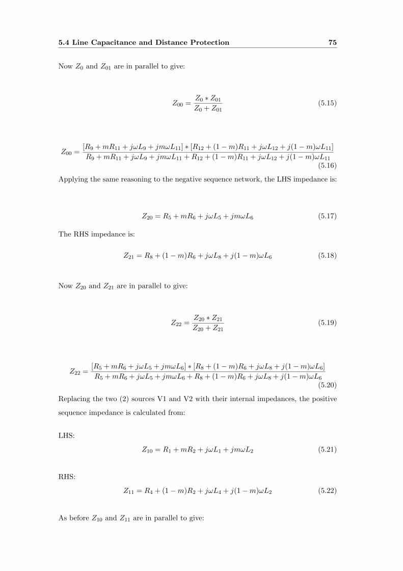
5.4 Line Capacitance and Distance Protection 75
Now Z0 and Z01 are in parallel to give:
Z00 =Z0 ∗ Z01
Z0 + Z01(5.15)
Z00 =[R9 +mR11 + jωL9 + jmωL11] ∗ [R12 + (1−m)R11 + jωL12 + j(1−m)ωL11]
R9 +mR11 + jωL9 + jmωL11 +R12 + (1−m)R11 + jωL12 + j(1−m)ωL11
(5.16)
Applying the same reasoning to the negative sequence network, the LHS impedance is:
Z20 = R5 +mR6 + jωL5 + jmωL6 (5.17)
The RHS impedance is:
Z21 = R8 + (1−m)R6 + jωL8 + j(1−m)ωL6 (5.18)
Now Z20 and Z21 are in parallel to give:
Z22 =Z20 ∗ Z21
Z20 + Z21(5.19)
Z22 =[R5 +mR6 + jωL5 + jmωL6] ∗ [R8 + (1−m)R6 + jωL8 + j(1−m)ωL6]
R5 +mR6 + jωL5 + jmωL6 +R8 + (1−m)R6 + jωL8 + j(1−m)ωL6
(5.20)
Replacing the two (2) sources V1 and V2 with their internal impedances, the positive
sequence impedance is calculated from:
LHS:
Z10 = R1 +mR2 + jωL1 + jmωL2 (5.21)
RHS:
Z11 = R4 + (1−m)R2 + jωL4 + j(1−m)ωL2 (5.22)
As before Z10 and Z11 are in parallel to give:
5.4 Line Capacitance and Distance Protection 76
Z111 =Z10 ∗ Z11
Z10 + Z11(5.23)
Z111 =[R1 +mR2 + jωL1 + jmωL2] ∗ [R4 + (1−m)R2 + jωL4 + j(1−m)ωL2]
R1 +mR2 + jωL1 + jmωL2 +R4 + (1−m)R2 + jωL4 + j(1−m)ωL2
(5.24)
The total impedance of the circuit is:
ZT = Z111 + Z22 + Z00 + 3Rf (5.25)
Thus
If =V1ZT
(5.26)
Hence
If = IAf = IBf = ICf =V1ZT
(5.27)
Equation 5.27 was plotted in Matlab to see how the impedance would vary with m.
In figure 5.6, a capacitor was introduced to the circuit to represent line capacitance
which would appear in a practical situation on a 500 kV line. A nominal π represen-
tation of the 500 kV line was drawn as shown Figure 5.7 . Capacitances C1/2 are
Figure 5.7: Equivalent circuit of phase A to ground with Capacitance Included
the positive sequence capacitances. C3/2 are the negative sequence capacitances and
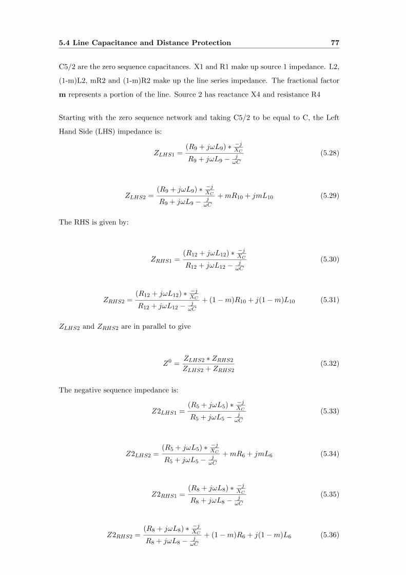
5.4 Line Capacitance and Distance Protection 77
C5/2 are the zero sequence capacitances. X1 and R1 make up source 1 impedance. L2,
(1-m)L2, mR2 and (1-m)R2 make up the line series impedance. The fractional factor
m represents a portion of the line. Source 2 has reactance X4 and resistance R4
Starting with the zero sequence network and taking C5/2 to be equal to C, the Left
Hand Side (LHS) impedance is:
ZLHS1 =(R9 + jωL9) ∗ −jXC
R9 + jωL9 − jωC
(5.28)
ZLHS2 =(R9 + jωL9) ∗ −jXC
R9 + jωL9 − jωC
+mR10 + jmL10 (5.29)
The RHS is given by:
ZRHS1 =(R12 + jωL12) ∗ −jXC
R12 + jωL12 − jωC
(5.30)
ZRHS2 =(R12 + jωL12) ∗ −jXC
R12 + jωL12 − jωC
+ (1−m)R10 + j(1−m)L10 (5.31)
ZLHS2 and ZRHS2 are in parallel to give
Z0 =ZLHS2 ∗ ZRHS2ZLHS2 + ZRHS2
(5.32)
The negative sequence impedance is:
Z2LHS1 =(R5 + jωL5) ∗ −jXC
R5 + jωL5 − jωC
(5.33)
Z2LHS2 =(R5 + jωL5) ∗ −jXC
R5 + jωL5 − jωC
+mR6 + jmL6 (5.34)
Z2RHS1 =(R8 + jωL8) ∗ −jXC
R8 + jωL8 − jωC
(5.35)
Z2RHS2 =(R8 + jωL8) ∗ −jXC
R8 + jωL8 − jωC
+ (1−m)R6 + j(1−m)L6 (5.36)
5.4 Line Capacitance and Distance Protection 78
But Z2LHS2 and Z2RHS2 are in parallel to give
Z2 =Z2LHS2 ∗ Z2RHS2Z2LHS2 + Z2RHS2
(5.37)
The positive sequence is obtained from:
Z1LHS1 =(R1 + jωL1) ∗ −jXC
R1 + jωL1 − jωC
(5.38)
Z1LHS2 =(R1 + jωL1) ∗ −jXC
R1 + jωL1 − jωC
+mR2 + jmL2 (5.39)
Z1RHS1 =(R4 + jωL4) ∗ −jXC
R4 + jωL4 − jωC
(5.40)
Z1RHS2 =(R4 + jωL4) ∗ −jXC
R4 + jωL4 − jωC
+ (1−m)R2 + j(1−m)L2 (5.41)
Again But Z1LHS2 and Z1RHS2 are in parallel to give
Z2 =Z1LHS2 ∗ Z1RHS2Z1LHS2 + Z1RHS2
(5.42)
The total impedance of the circuit is:
ZT = Z0 + Z1 + Z2 + 3Rf (5.43)
Thus
If =V1ZT
(5.44)
Hence
If = IAf = IBf = ICf =V1ZT
(5.45)
It can be seen that line capacitance C is affecting ZT the impedance seen by the relay
at the fault point. The impedance varies as m changes.
5.5 Chapter Summary 79
5.5 Chapter Summary
It has be seen observed that line capacitance C is affecting ZT the impedance seen by
the relay at the fault point. The impedance varies as m is varied along the length of
the line.
Because line capacitance affects the currents flowing along the line, the capacitive
currents have to be compensated for if a current differential protection is to be used.
Chapter 6
Protection Relay
6.1 Chapter Overview
This chapter looks in detail the relays SEL (Schweitzer Engineering Laboratories) 311L
relay, GE (General Electric) Multilin L90 and Siemens 7SD5. Specifics of how these
individual relays operate will be analysed.
Relay manufactures have different ways of implementing power systems protection func-
tions in numeric relays. A detailed study of a particular relay helps the user to identify
the limits of that brand of relay to the intended protection functions. This chapter is
seeking to identify these limitations whilst seeking the best out of the relay.
6.2 SEL 311L
The SEL (Schweitzer Engineering Laboratories)relay houses current differential protec-
tion and distance protection. It has back up protections such as:
• over current protection.
• instantaneous or definite time over current protection.
• out of step protection.
• frequency elements
6.2 SEL 311L 81
• loss of potential protection.
• negative sequence protection.
• directional earth fault protection.
The relay also has control functions such as synchronism of networks, auto re-close op-
erations. The relay provides metering of the measured voltages, currents and frequency.
The relay has front panel push buttons where the user can access different metering
options. The relay has an inbuilt fault recorder that reports and logs event reports
(Schweitzer Engineering Laboratories 2003). The relay has a password protection sys-
tem to prevent anyone else from accessing the settings.
Figure 6.1 shows the connection diagram for a SEL311L relay to provide current dif-
ferential and distance protection. The CTs are connected with the star point towards
the line. This is the tripping direction. 52 is the CB and 52A is CB normally open
auxiliary contact, 52B is CB normally closed auxiliary contact. CH X and CH Y are
two independent communication channels used for inter relay communications.
6.2.1 Current Differential Protection
The principle of operation of the current differential relay is that currents flowing into
the protected line are assigned angle zero and the currents flowing out of the protected
line is assigned angle 180 degrees (Schweitzer Engineering Laboratories 2003) . Suppose
a 1 amp load current is flowing into the line. The relay then calculates the ratio of
remote current to local current as shown in equation 6.1
IRLL
=16 180
1 6 0(6.1)
The result is a point at 1 6 180. All phases do the same calculation and the result is a
point at 1 6 180. The relay then surrounds this point with a region called the restrain
region. The relay issues a trip when an operating point travels outside this region.
The differential characteristic is shown in figure 6.2. 87LANG describes the angular
extend of the restrain region and 87LR determines the outer radius of the region. The
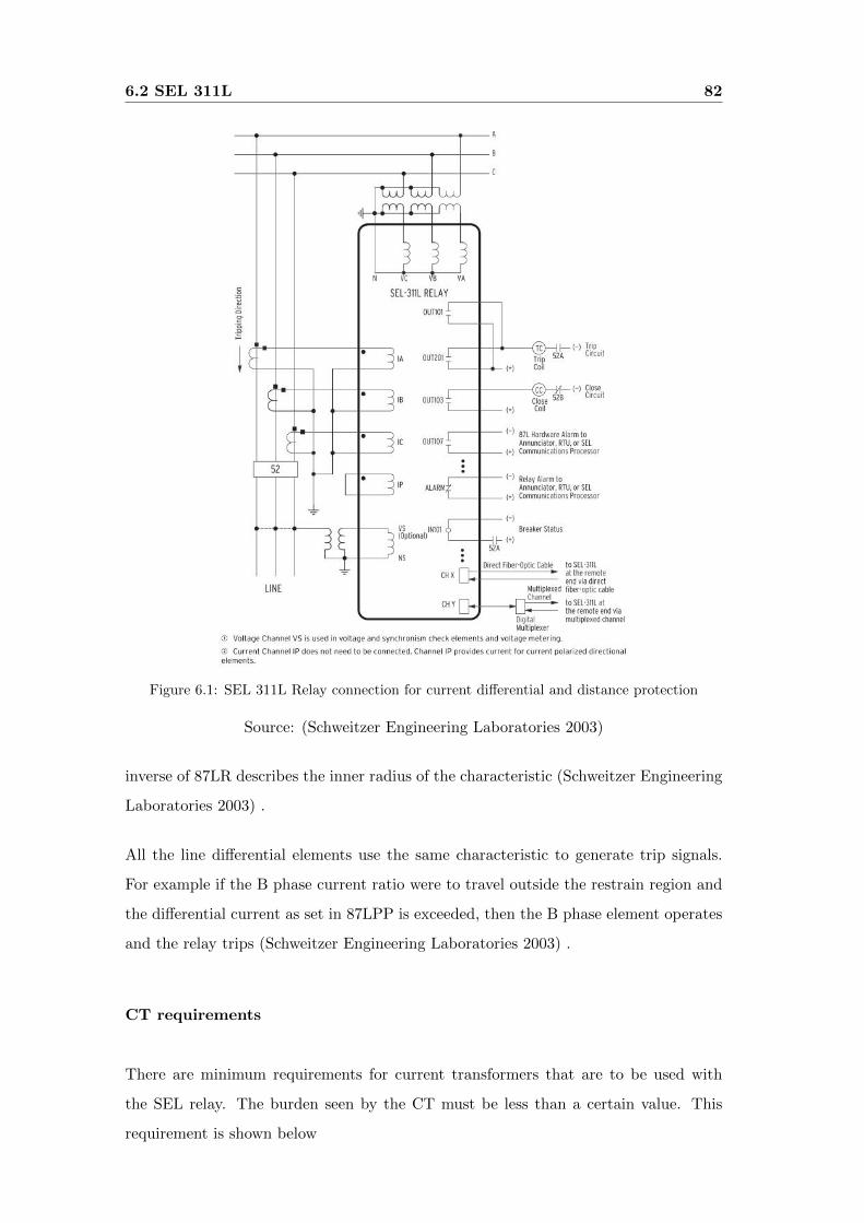
6.2 SEL 311L 82
Figure 6.1: SEL 311L Relay connection for current differential and distance protection
Source: (Schweitzer Engineering Laboratories 2003)
inverse of 87LR describes the inner radius of the characteristic (Schweitzer Engineering
Laboratories 2003) .
All the line differential elements use the same characteristic to generate trip signals.
For example if the B phase current ratio were to travel outside the restrain region and
the differential current as set in 87LPP is exceeded, then the B phase element operates
and the relay trips (Schweitzer Engineering Laboratories 2003) .
CT requirements
There are minimum requirements for current transformers that are to be used with
the SEL relay. The burden seen by the CT must be less than a certain value. This
requirement is shown below
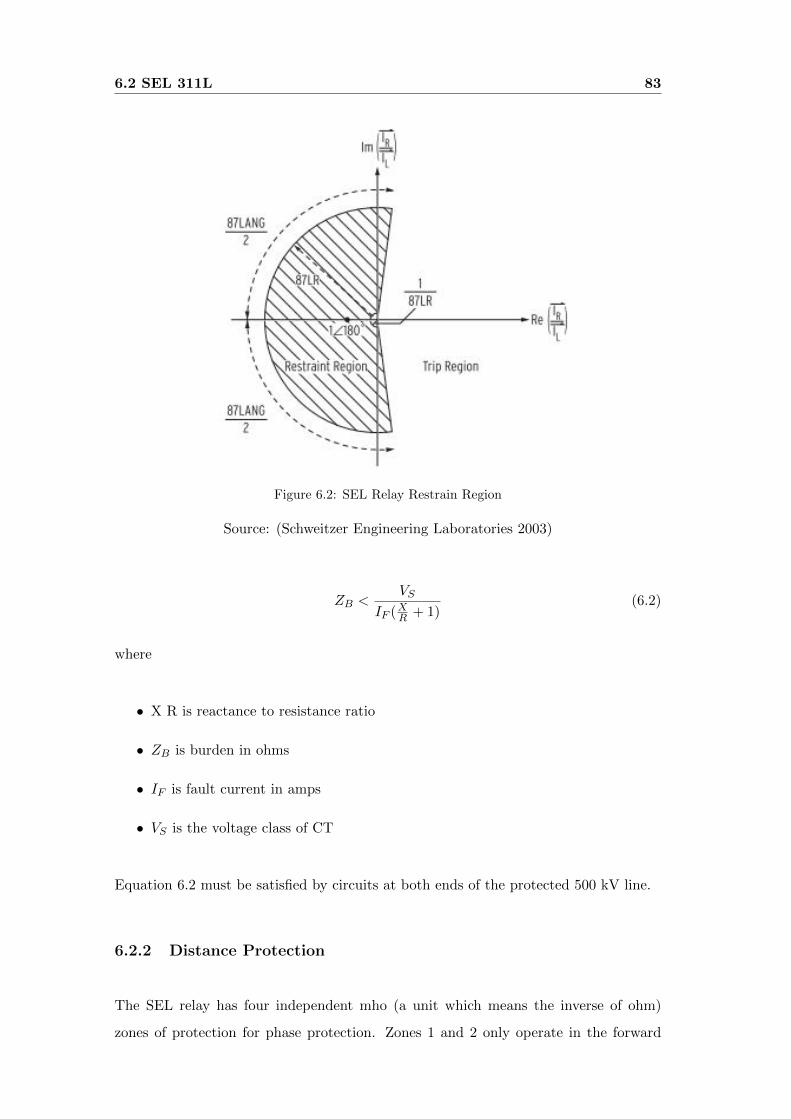
6.2 SEL 311L 83
Figure 6.2: SEL Relay Restrain Region
Source: (Schweitzer Engineering Laboratories 2003)
ZB <VS
IF (XR + 1)(6.2)
where
• X R is reactance to resistance ratio
• ZB is burden in ohms
• IF is fault current in amps
• VS is the voltage class of CT
Equation 6.2 must be satisfied by circuits at both ends of the protected 500 kV line.
6.2.2 Distance Protection
The SEL relay has four independent mho (a unit which means the inverse of ohm)
zones of protection for phase protection. Zones 1 and 2 only operate in the forward
6.2 SEL 311L 84
direction whereas zones 3 and 4 can either be forward or reverse looking. All types of
faults are covered, phase to ground, phase to phase and phase to phase to ground.
A 500 kV line must be protected against all types of faults. The most common fault
is phase to ground. Phase to phase is not very common on a 500 kV line because the
conductors are spaced at greater distances for them to touch one another. According
to Donald & Maceau (2006) failures of transmission lines are caused by events such as
bad weather, equipment faults and human error. An analysis of faults indicate that
phase to ground faults are very common (more than 95 percent)while very rarely three
phase faults caused by forest fires can also occur.
Statistics of transmission line faults show that the percentage of single phase faults
increase with nominal voltage and the the dimensions of the line i.e. from 60 percent at
220 kV to 97 percent for 735 kV lines. To improve stability, single phase auto-reclose
(SPR) has been adopted (Donald & Maceau 2006) . In this project, a fully functional
500 kV line protection involves the inclusion of properly set high speed auto re-close
relay.
The principle of operation of the SEL distance relay involves sampling the voltages and
currents presented to the relay. The relay samples the most recent current or voltage
vector and calls it the real part, then a sample taken a quarter of the period earlier is
called the imaginary part (Schweitzer Engineering Laboratories 2003) .
V 1 = V1 6 Θ (6.3)
V 2 = V2 6 Θ (6.4)
Now the relay needs to calculate 6 (Θ1 -Θ2)
To do this, Schweitzer Engineering Laboratories (2003) takes the conjugate of V2 6 Θ
and multiplies this quantity by V1 6 Θ using complex numbers to get V3
V 3 = V 1 ∗ V 2′ 6 (Θ1 −Θ2) (6.5)
6.2 SEL 311L 85
The cosine of V3 is then assigned the real part and the sine of V3 is assigned the imag-
inary part. To calculate Z, the impedance reach, Schweitzer Engineering Laboratories
(2003) uses the equation:
0 = Rel[(Z ∗ I − V ) ∗ V1mem] (6.6)
Where
• Rel means real part
• I is the current flowing in the circuit
• V1mem is the polarising voltage
The quantity Z ∗ I − V is called the line drop compensated voltage. The use of such
a quantity makes sense because this is a value obtained from a known current flowing
through an impedance of particular interest namely Z.
For an AB phase fault, the torque calculation for a positive sequence polarised mho
represented by mAB is given by:
mAB =Re(VAB ∗ VAB1mem)
Rel(16 Z ∗ IAB ∗ VAB1mem)(6.7)
Similary for a BC phase fault the torque calculation for a positive sequence polarised
mho represented by mBC is given by:
mBC =Re(VBC ∗ VBC1mem)
Rel(16 Z ∗ IBC ∗ VBC1mem)(6.8)
For a CA phase fault, the torque calculation for a positive sequence polarised mho
represented by mCA is given by:
mCA =Re(VCA ∗ VCA1mem)
Rel(16 Z ∗ ICA ∗ VCA1mem)(6.9)
The phase to phase counterpart for the compensator distance mho element is given by:
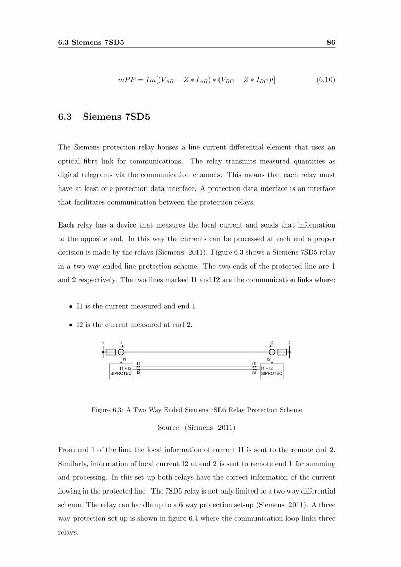
6.3 Siemens 7SD5 86
mPP = Im[(VAB − Z ∗ IAB) ∗ (VBC − Z ∗ IBC)′] (6.10)
6.3 Siemens 7SD5
The Siemens protection relay houses a line current differential element that uses an
optical fibre link for communications. The relay transmits measured quantities as
digital telegrams via the communication channels. This means that each relay must
have at least one protection data interface. A protection data interface is an interface
that facilitates communication between the protection relays.
Each relay has a device that measures the local current and sends that information
to the opposite end. In this way the currents can be processed at each end a proper
decision is made by the relays (Siemens 2011). Figure 6.3 shows a Siemens 7SD5 relay
in a two way ended line protection scheme. The two ends of the protected line are 1
and 2 respectively. The two lines marked I1 and I2 are the communication links where:
• I1 is the current measured and end 1
• I2 is the current measured at end 2.
Figure 6.3: A Two Way Ended Siemens 7SD5 Relay Protection Scheme
Source: (Siemens 2011)
From end 1 of the line, the local information of current I1 is sent to the remote end 2.
Similarly, information of local current I2 at end 2 is sent to remote end 1 for summing
and processing. In this set up both relays have the correct information of the current
flowing in the protected line. The 7SD5 relay is not only limited to a two way differential
scheme. The relay can handle up to a 6 way protection set-up (Siemens 2011). A three
way protection set-up is shown in figure 6.4 where the communication loop links three
relays.
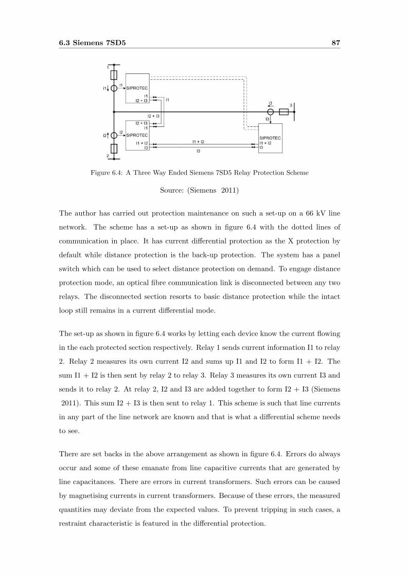
6.3 Siemens 7SD5 87
Figure 6.4: A Three Way Ended Siemens 7SD5 Relay Protection Scheme
Source: (Siemens 2011)
The author has carried out protection maintenance on such a set-up on a 66 kV line
network. The scheme has a set-up as shown in figure 6.4 with the dotted lines of
communication in place. It has current differential protection as the X protection by
default while distance protection is the back-up protection. The system has a panel
switch which can be used to select distance protection on demand. To engage distance
protection mode, an optical fibre communication link is disconnected between any two
relays. The disconnected section resorts to basic distance protection while the intact
loop still remains in a current differential mode.
The set-up as shown in figure 6.4 works by letting each device know the current flowing
in the each protected section respectively. Relay 1 sends current information I1 to relay
2. Relay 2 measures its own current I2 and sums up I1 and I2 to form I1 + I2. The
sum I1 + I2 is then sent by relay 2 to relay 3. Relay 3 measures its own current I3 and
sends it to relay 2. At relay 2, I2 and I3 are added together to form I2 + I3 (Siemens
2011). This sum I2 + I3 is then sent to relay 1. This scheme is such that line currents
in any part of the line network are known and that is what a differential scheme needs
to see.
There are set backs in the above arrangement as shown in figure 6.4. Errors do always
occur and some of these emanate from line capacitive currents that are generated by
line capacitances. There are errors in current transformers. Such errors can be caused
by magnetising currents in current transformers. Because of these errors, the measured
quantities may deviate from the expected values. To prevent tripping in such cases, a
restraint characteristic is featured in the differential protection.
6.3 Siemens 7SD5 88
The line charging currents that appear on a 500 kV line will have to be compensated
by the relay for the protection to function correctly. Equation 6.11 defines the zero
sequence capacitor current and this has to be set in the relay. Table ?? shows the
positive and zero sequence capacitances of the 500 kV line of this project.
IC0 = 2 ∗ π ∗ f ∗ C0 ∗ V (6.11)
IC0 = 2 ∗ π ∗ 50 ∗ 0.00798 ∗ 10−6 ∗ 288.675 ∗ 103 ∗ L (6.12)
IC0 = 19.12A (6.13)
Where V is the phase to ground voltage and L is the length of the line. L is equal to
83 kilo metres (km). So the primary zero sequence capacitive current is 19.12 amps.
The positive sequence capacitive current is:
IC+ = 2 ∗ π ∗ f ∗ C+ ∗ V (6.14)
IC+ = 2 ∗ π ∗ 50 ∗ 0.0207 ∗ 10−6 ∗ 288.675 ∗ 103 ∗ L (6.15)
IC+ = 49.6 (6.16)
The capacitive current in this case is 50 amps and this has to be compensated for. If
no compensation is to be done, then the capacitive current has to be included in the
calculation of the differential relay pick up current.
6.3.1 Further influences
There are other effects that can cause errors in the relay operation (Siemens 2011).
These are:
• hardware tolerances.
• calculation tolerances.
• deviations in time.
• deviations in frequency.
Deviations in time are caused by errors in synchronisation of the measured quantities
and data transmission and operating time variations. The 7SD5 relay does not actually
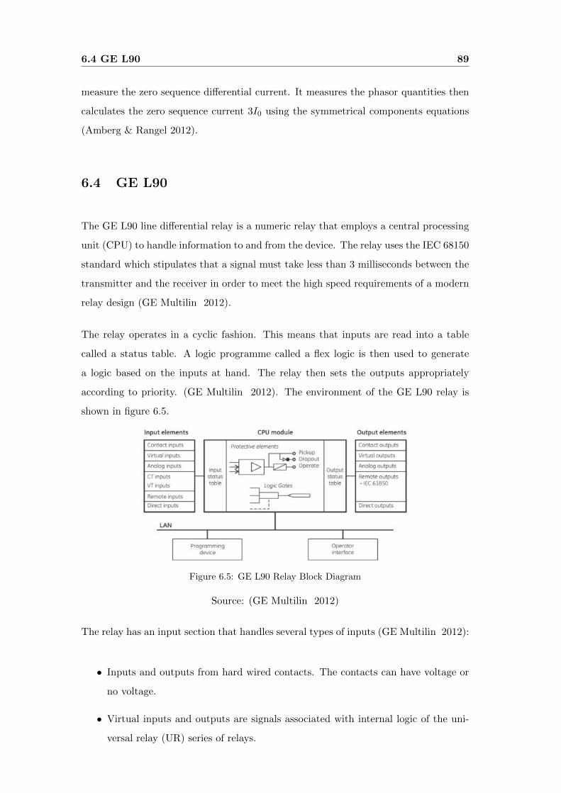
6.4 GE L90 89
measure the zero sequence differential current. It measures the phasor quantities then
calculates the zero sequence current 3I0 using the symmetrical components equations
(Amberg & Rangel 2012).
6.4 GE L90
The GE L90 line differential relay is a numeric relay that employs a central processing
unit (CPU) to handle information to and from the device. The relay uses the IEC 68150
standard which stipulates that a signal must take less than 3 milliseconds between the
transmitter and the receiver in order to meet the high speed requirements of a modern
relay design (GE Multilin 2012).
The relay operates in a cyclic fashion. This means that inputs are read into a table
called a status table. A logic programme called a flex logic is then used to generate
a logic based on the inputs at hand. The relay then sets the outputs appropriately
according to priority. (GE Multilin 2012). The environment of the GE L90 relay is
shown in figure 6.5.
Figure 6.5: GE L90 Relay Block Diagram
Source: (GE Multilin 2012)
The relay has an input section that handles several types of inputs (GE Multilin 2012):
• Inputs and outputs from hard wired contacts. The contacts can have voltage or
no voltage.
• Virtual inputs and outputs are signals associated with internal logic of the uni-
versal relay (UR) series of relays.
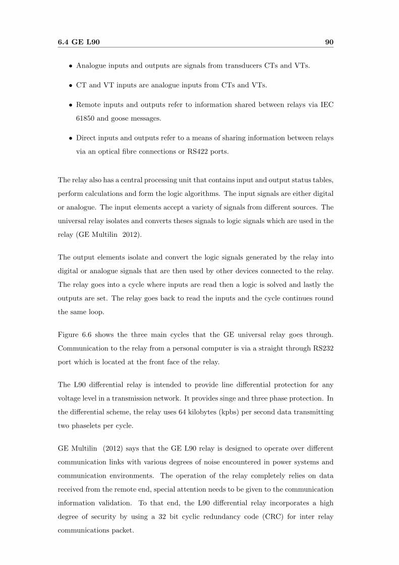
6.4 GE L90 90
• Analogue inputs and outputs are signals from transducers CTs and VTs.
• CT and VT inputs are analogue inputs from CTs and VTs.
• Remote inputs and outputs refer to information shared between relays via IEC
61850 and goose messages.
• Direct inputs and outputs refer to a means of sharing information between relays
via an optical fibre connections or RS422 ports.
The relay also has a central processing unit that contains input and output status tables,
perform calculations and form the logic algorithms. The input signals are either digital
or analogue. The input elements accept a variety of signals from different sources. The
universal relay isolates and converts theses signals to logic signals which are used in the
relay (GE Multilin 2012).
The output elements isolate and convert the logic signals generated by the relay into
digital or analogue signals that are then used by other devices connected to the relay.
The relay goes into a cycle where inputs are read then a logic is solved and lastly the
outputs are set. The relay goes back to read the inputs and the cycle continues round
the same loop.
Figure 6.6 shows the three main cycles that the GE universal relay goes through.
Communication to the relay from a personal computer is via a straight through RS232
port which is located at the front face of the relay.
The L90 differential relay is intended to provide line differential protection for any
voltage level in a transmission network. It provides singe and three phase protection. In
the differential scheme, the relay uses 64 kilobytes (kpbs) per second data transmitting
two phaselets per cycle.
GE Multilin (2012) says that the GE L90 relay is designed to operate over different
communication links with various degrees of noise encountered in power systems and
communication environments. The operation of the relay completely relies on data
received from the remote end, special attention needs to be given to the communication
information validation. To that end, the L90 differential relay incorporates a high
degree of security by using a 32 bit cyclic redundancy code (CRC) for inter relay
communications packet.
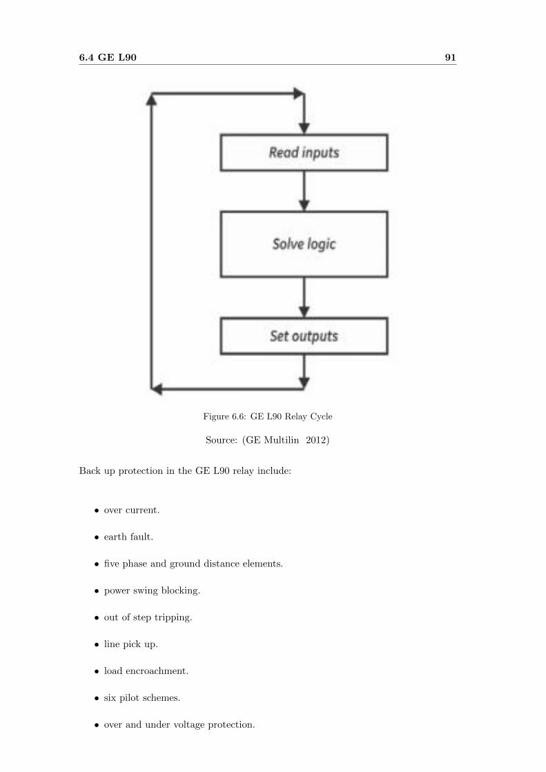
6.4 GE L90 91
Figure 6.6: GE L90 Relay Cycle
Source: (GE Multilin 2012)
Back up protection in the GE L90 relay include:
• over current.
• earth fault.
• five phase and ground distance elements.
• power swing blocking.
• out of step tripping.
• line pick up.
• load encroachment.
• six pilot schemes.
• over and under voltage protection.
6.4 GE L90 92
For long transmission lines such as a 500 kV overhead line, the GE L90 relay provides
line charging current compensation such that the line charging current is removed from
the line terminal phasors (GE Multilin 2012) . The relay also provides secure protection
when used in breaker and half schemes.
Additional protection provided by the relay include:
• Voltage transformer and current transformer supervision.
• Breaker failure protection.
• Stub bus protection.
• Open pole detection.
• Trip coil supervision.
• Creation of a user defined flex logic to manipulate relay functions.
The relay also provides control to a circuit breaker used either in a 500 kV ring or a 500
kV breaker and half scheme by a push button controls in the relay. The relay has an
inbuilt auto re-closing relay and a synchronising relay. The relay monitors the breaker
arcing current (GE Multilin 2012) . The GE L90 relay also has a monitoring facility
where voltage and current waveforms are plotted, up to 1024 events are stored. A fault
locator is also included in the package.
The GE L90 relay meters all the 87L phasors, channel delays and channel asymmetry.
Other measurements done by the relay include line currents, voltage, real power, ap-
parent power, power factor and frequency. There is an RS232 communications port at
front the front of the relay and this has a capacity of 19.2 kbps. There is a rear RS485
port with a capability of 115 kbps. There is an ethernet port at the back of the relay
and this one supports the IEC 61850 protocol.
The GE L90 relay has a dedicated optical fibre communication link which operates at
64 kbps. The available interfaces are RS422 and G.703 at 64 kbps (GE Multilin 2012)
. The options for the fibre optic connections are;
• 820 nano metre (nm) multi-mode optic fibre with LED (light emitting diode)
transmitter.
6.4 GE L90 93
• 1300 nm multi-mode fibre with LED transmitter.
• 1300 nm single-mode fibre with ELED transmitter.
• 1300 nm single-mode fibre with laser (light activation by stimulated emission of
radiation) transmitter.
• 1550 nm single-mode fibre with laser transmitter.
• IEEE C.37.94 8200 nm single-mode fibre with LED transmitter.
When the relay is used in a two terminal network, a second bidirectional channel can
be used as a redundant communication channel. The L90 relay can work in a peer to
peer network or a master to peer relation. In the peer to peer architecture, all relays
are the same and perform identical current differential functions (GE Multilin 2012)
. In a master to peer architecture, the master relay has the current phasors from the
other relays.
In a master to peer set up, the master relay performs the actual line current differential
calculations and only the master will communicate with the other relays in the loop.
The slave relays only communicate with the master. this means that when a master
relay issues a local trip signal, it sends a command called a direct transfer trip (DTT)
to remote terminals so that they trip their local breakers as well.
When a slave relays issues a local trip from one of its back up protections, it can send
a trip to the master and the master will broadcast the trip to all the relays in the loop.
This is because a slave does not communicate with all relays in the loop. The author
feels that this set up is not very good. On a 500 kV line network, tripping time is very
important. The author strongly believes that sending trip signal to the master relay
first is simply wasting valuable time and is not necessary. The author also believes the
mater relay is given too much control than is necessary. The master relay is the only one
doing the line current differential calculations while the other relays are seated doing
very little - this is not a good option to choose. If the master relay looses accuracy and
is calculating fault data wrongly, then the whole protection scheme fails. A wrong trip
may be broadcast to all relays in the loop. This is bad for a heavily loaded 500 kV line
supplying power to important installations such as hospitals, fire fighting plants, water
treatment plants and many more.
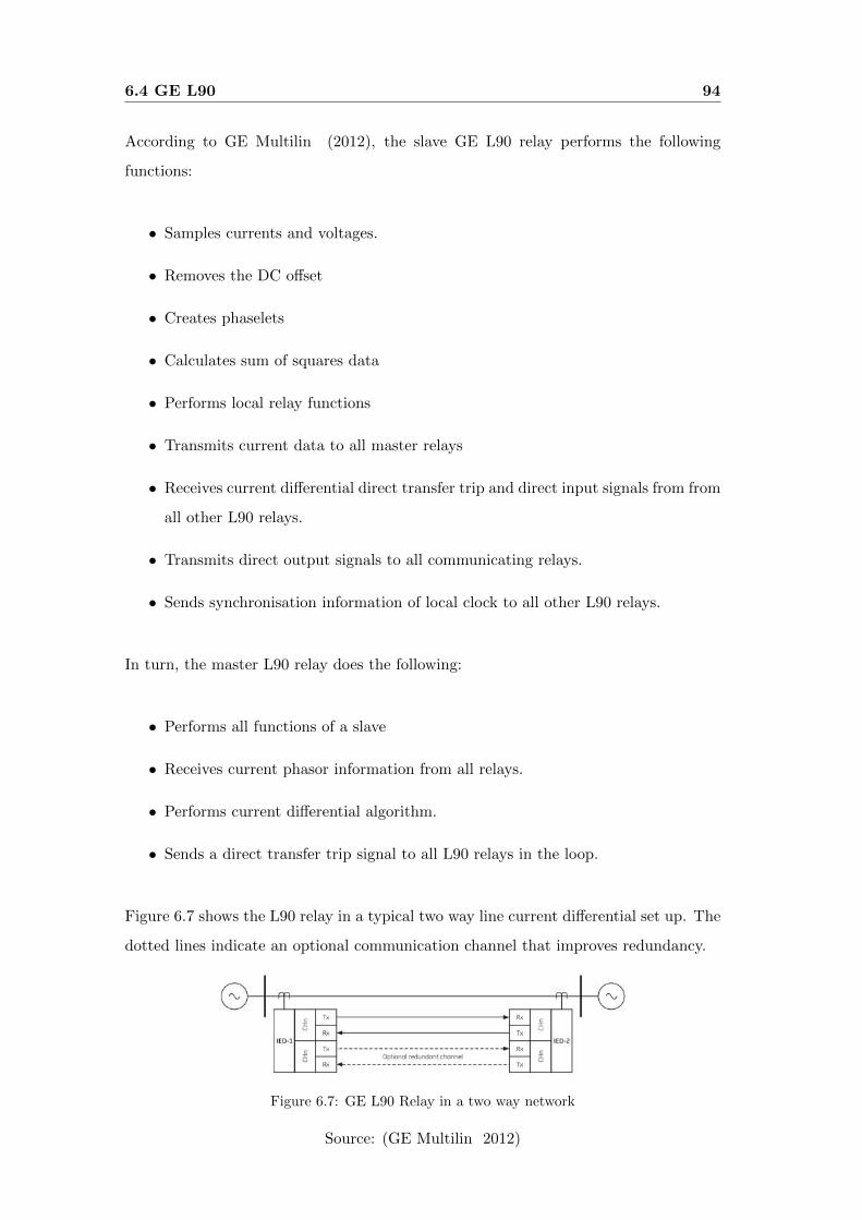
6.4 GE L90 94
According to GE Multilin (2012), the slave GE L90 relay performs the following
functions:
• Samples currents and voltages.
• Removes the DC offset
• Creates phaselets
• Calculates sum of squares data
• Performs local relay functions
• Transmits current data to all master relays
• Receives current differential direct transfer trip and direct input signals from from
all other L90 relays.
• Transmits direct output signals to all communicating relays.
• Sends synchronisation information of local clock to all other L90 relays.
In turn, the master L90 relay does the following:
• Performs all functions of a slave
• Receives current phasor information from all relays.
• Performs current differential algorithm.
• Sends a direct transfer trip signal to all L90 relays in the loop.
Figure 6.7 shows the L90 relay in a typical two way line current differential set up. The
dotted lines indicate an optional communication channel that improves redundancy.
Figure 6.7: GE L90 Relay in a two way network
Source: (GE Multilin 2012)
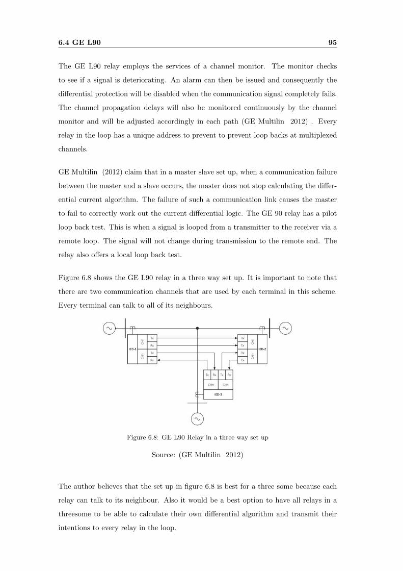
6.4 GE L90 95
The GE L90 relay employs the services of a channel monitor. The monitor checks
to see if a signal is deteriorating. An alarm can then be issued and consequently the
differential protection will be disabled when the communication signal completely fails.
The channel propagation delays will also be monitored continuously by the channel
monitor and will be adjusted accordingly in each path (GE Multilin 2012) . Every
relay in the loop has a unique address to prevent to prevent loop backs at multiplexed
channels.
GE Multilin (2012) claim that in a master slave set up, when a communication failure
between the master and a slave occurs, the master does not stop calculating the differ-
ential current algorithm. The failure of such a communication link causes the master
to fail to correctly work out the current differential logic. The GE 90 relay has a pilot
loop back test. This is when a signal is looped from a transmitter to the receiver via a
remote loop. The signal will not change during transmission to the remote end. The
relay also offers a local loop back test.
Figure 6.8 shows the GE L90 relay in a three way set up. It is important to note that
there are two communication channels that are used by each terminal in this scheme.
Every terminal can talk to all of its neighbours.
Figure 6.8: GE L90 Relay in a three way set up
Source: (GE Multilin 2012)
The author believes that the set up in figure 6.8 is best for a three some because each
relay can talk to its neighbour. Also it would be a best option to have all relays in a
threesome to be able to calculate their own differential algorithm and transmit their
intentions to every relay in the loop.
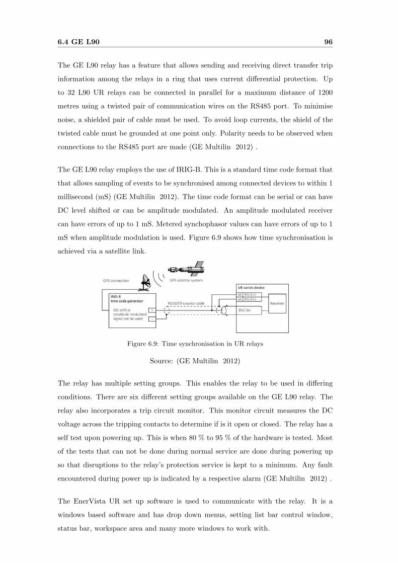
6.4 GE L90 96
The GE L90 relay has a feature that allows sending and receiving direct transfer trip
information among the relays in a ring that uses current differential protection. Up
to 32 L90 UR relays can be connected in parallel for a maximum distance of 1200
metres using a twisted pair of communication wires on the RS485 port. To minimise
noise, a shielded pair of cable must be used. To avoid loop currents, the shield of the
twisted cable must be grounded at one point only. Polarity needs to be observed when
connections to the RS485 port are made (GE Multilin 2012) .
The GE L90 relay employs the use of IRIG-B. This is a standard time code format that
that allows sampling of events to be synchronised among connected devices to within 1
millisecond (mS) (GE Multilin 2012). The time code format can be serial or can have
DC level shifted or can be amplitude modulated. An amplitude modulated receiver
can have errors of up to 1 mS. Metered synchophasor values can have errors of up to 1
mS when amplitude modulation is used. Figure 6.9 shows how time synchronisation is
achieved via a satellite link.
Figure 6.9: Time synchronisation in UR relays
Source: (GE Multilin 2012)
The relay has multiple setting groups. This enables the relay to be used in differing
conditions. There are six different setting groups available on the GE L90 relay. The
relay also incorporates a trip circuit monitor. This monitor circuit measures the DC
voltage across the tripping contacts to determine if is it open or closed. The relay has a
self test upon powering up. This is when 80 % to 95 % of the hardware is tested. Most
of the tests that can not be done during normal service are done during powering up
so that disruptions to the relay’s protection service is kept to a minimum. Any fault
encountered during power up is indicated by a respective alarm (GE Multilin 2012) .
The EnerVista UR set up software is used to communicate with the relay. It is a
windows based software and has drop down menus, setting list bar control window,
status bar, workspace area and many more windows to work with.
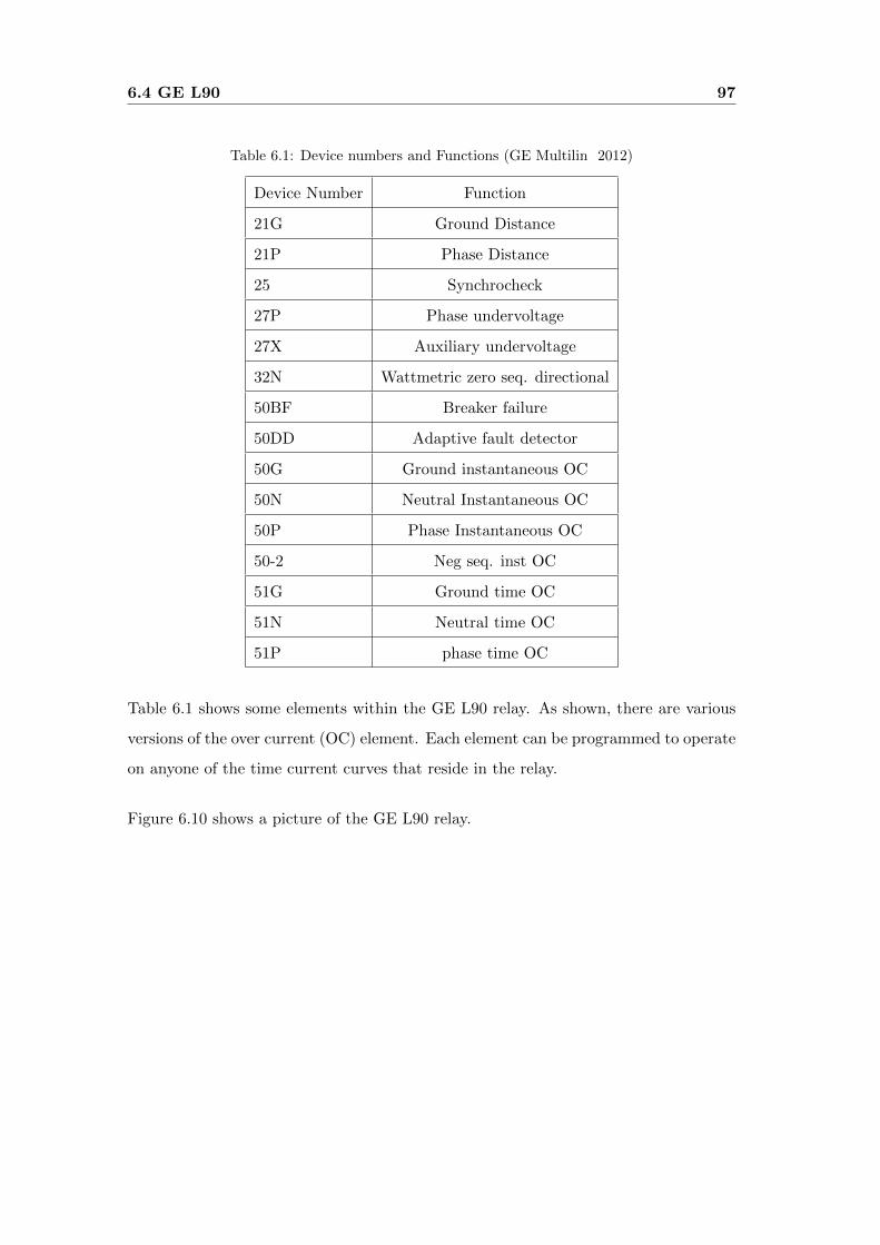
6.4 GE L90 97
Table 6.1: Device numbers and Functions (GE Multilin 2012)
Device Number Function
21G Ground Distance
21P Phase Distance
25 Synchrocheck
27P Phase undervoltage
27X Auxiliary undervoltage
32N Wattmetric zero seq. directional
50BF Breaker failure
50DD Adaptive fault detector
50G Ground instantaneous OC
50N Neutral Instantaneous OC
50P Phase Instantaneous OC
50-2 Neg seq. inst OC
51G Ground time OC
51N Neutral time OC
51P phase time OC
Table 6.1 shows some elements within the GE L90 relay. As shown, there are various
versions of the over current (OC) element. Each element can be programmed to operate
on anyone of the time current curves that reside in the relay.
Figure 6.10 shows a picture of the GE L90 relay.
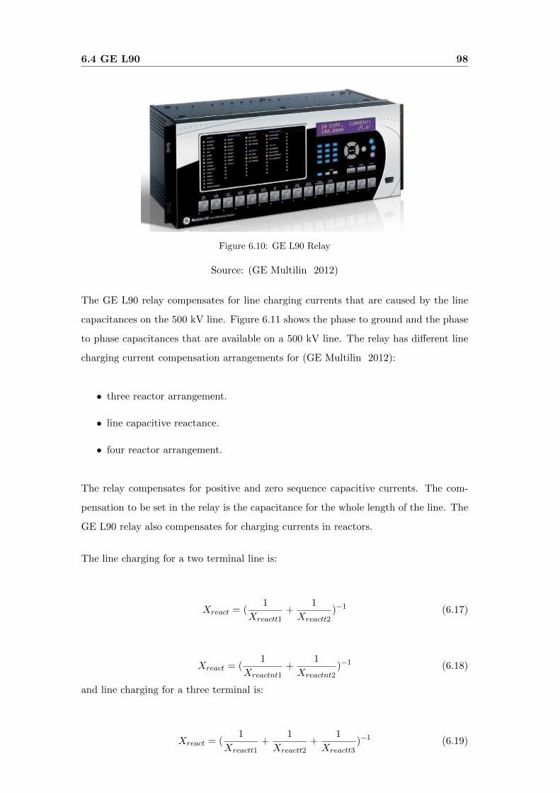
6.4 GE L90 98
Figure 6.10: GE L90 Relay
Source: (GE Multilin 2012)
The GE L90 relay compensates for line charging currents that are caused by the line
capacitances on the 500 kV line. Figure 6.11 shows the phase to ground and the phase
to phase capacitances that are available on a 500 kV line. The relay has different line
charging current compensation arrangements for (GE Multilin 2012):
• three reactor arrangement.
• line capacitive reactance.
• four reactor arrangement.
The relay compensates for positive and zero sequence capacitive currents. The com-
pensation to be set in the relay is the capacitance for the whole length of the line. The
GE L90 relay also compensates for charging currents in reactors.
The line charging for a two terminal line is:
Xreact = (1
Xreactt1+
1
Xreactt2)−1 (6.17)
Xreact = (1
Xreactnt1+
1
Xreactnt2)−1 (6.18)
and line charging for a three terminal is:
Xreact = (1
Xreactt1+
1
Xreactt2+
1
Xreactt3)−1 (6.19)
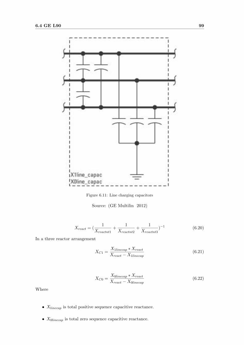
6.4 GE L90 99
Figure 6.11: Line charging capacitors
Source: (GE Multilin 2012)
Xreact = (1
Xreactnt1+
1
Xreactnt2+
1
Xreactnt3)−1 (6.20)
In a three reactor arrangement
XC1 =X1linecap ∗Xreact
Xreact −X1linecap(6.21)
XC0 =X0linecap ∗Xreact
Xreact −X0linecap(6.22)
Where
• Xlinecap is total positive sequence capacitive reactance.
• X0linecap is total zero sequence capacitive reactance.
6.4 GE L90 100
• Xreact is total inductive reactance per phase. For two identical reactances at each
end of the line, the value of reactance is divided by 2 or 3 depending on number
of line terminals.
• Xreactn is total neutral inductive reactance per phase. For two identical reactances
at each end of the line, the value of reactance is divided by 2 or 3 depending on
number of line terminals.
The GE L90 relay has a common setting for the distance elements. This is the distance
source that defines the source of the voltage provided to the distance elements. The
mho unit uses either the positive sequence voltage or a memorised voltage. There is a
time setting which determines how long the memorised voltage can be used in distance
calculations. When this time expires, the relay checks to see if the positive sequence
voltage is higher than 10 %. If it is, then the positive sequence voltage is used (GE
Multilin 2012) . If not, then the memorised voltage will continue to be used. The
memory is established whenever the voltage gets to 80 % of its nominal value for five
power frequency cycles.
There is an option to use either memory voltage polarisation or self polarisation. The
memory duration must be set long enough to cater for close in reverse three phase faults.
Because of this, the circuit breaker maximum fault clearing time must be known. At
the same time, the memory voltage can not be kept frozen for too long because that
will not represent the actual system voltage.
Figure 6.12 shows a directional mho characteristic curve of the GE L90 relay. All phase
distance elements of this relay are reversible. Some points to note on the characteristic
plot are:
• Phs Dist Z1 Reach refers to zone one (1) forward reach.
• Phs Dist Z1 RCA refers to zone one (1) characteristic angle.
• Phs Dist Z1 Comp Limit refers to the shape of zone one (1) operating character-
istic.
• Phs Dist Z1 Dir refers to RCA refers to the characteristic angle of the directional
supervising function.
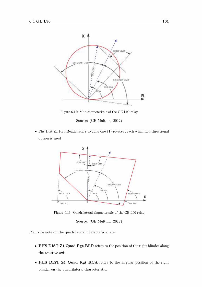
6.4 GE L90 101
Figure 6.12: Mho characteristic of the GE L90 relay
Source: (GE Multilin 2012)
• Phs Dist Z1 Rev Reach refers to zone one (1) reverse reach when non directional
option is used
Figure 6.13: Quadrilateral characteristic of the GE L90 relay
Source: (GE Multilin 2012)
Points to note on the quadrilateral characteristic are:
• PHS DIST Z1 Quad Rgt BLD refers to the position of the right blinder along
the resistive axis.
• PHS DIST Z1 Quad Rgt RCA refers to the angular position of the right
blinder on the quadrilateral characteristic.
6.4 GE L90 102
• PHS DIST Z1 Quad LFT BLD refers to the position of the left blinder along
the resistive axis.
• PHS DIST Z1 Quad LFT RCA refers to the angular position of the left
blinder along the resistive axis.
The GE L90 relay removes the DC component from its measured quantities. This re-
duces measurement errors that are caused by the inductive behaviour of a transmission
line once a voltage is applied to the line (GE Multilin 2012) . An advantage of this is
that there is less overshoot of the measured quantities (typically less than 2 %) regard-
less of the time constant of the initial magnitude and time constant of the DC offset.
This means that the measured quantity is very nearly its true value whenever the relay
is taking measurements.
6.5 Chapter Summary 103
6.5 Chapter Summary
This chapter has looked at the line differential characteristic of the SEL relay. A ratio
of remote to local currents is calculated. This ratio is used in defining the restraining
region. The characteristic plot is defined by the angle coverage of the restrain region
and the radius of the restrain region LR. The relay avoids restraining faults close to
the origin by using the inverse of the restraining radius 1/LR
Distance relay characteristics of the GE L90 relay have been analysed. The relay has
both quadrilateral and mho characteristics that can be programmed to look in any
intended direction. The power swing block element in the L90 relay has a variety of
settings that can suit almost any likely power swing disturbance.
The Siemens 7SD5 relay has a simple line differential characteristic curve. The fault
locator and the event recorder in this relay is very flexible and more user friendly when
retrieving fault information. The three way differential set up has a good optical fibre
link data distribution such that line currents in any part of the loop are known.
Chapter 7
Systematic Procedure To
Determine Relay Settings
7.1 Chapter Overview
This chapter will look at different procedures that can be adopted by any power utility
in order to come up with a procedure to determine line protection settings on a 500 kV
line. Firstly, the Aspen Software will be discussed. This software tool incorporates a
database where relay information can be stored.
Next will be the discussion on implementing settings in the relays SEL (Shweitzer
Engineering Laboratories) 311L, GE (General Electric) Multilin L90 and the Siemens
7SD5 relays. Distance protection and line current differential settings will be included
for each relay.
7.2 ASPEN Software for Relay Database
There are several procedures currently in use by various power utilities throughout the
world to determine, preserve and manage relay settings. One such programme is the
Aspen software. This software has a database for storing relay information and related
protection equipment. Any type of relay from electromechanical ones with few setting
parameters to modern day microprocessor relays with thousands of parameters can be
7.2 ASPEN Software for Relay Database 105
stored on this database (Aspen 2013).
The database is very flexible in that for any relay, multiple sets of setting values can be
stored. Some of these settings can be for historical purposes. Other settings could be
for emergency purposes or some settings will be there in the database pending approval.
Aspen (2013) database also lets users store information on circuit breakers (CBs), power
transformers, current transformers (CTs), voltage transformers and communications
equipment.
There is a task module in that database that allows users to store and follow up a huge
variety of activities related to relay settings, tests and protection system maintenance.
Each task can have an unlimited number of activities and events. In the task module,
a protection maintenance plan can be set up and accurate records of work done can be
easily retrieved.
The software has a built in reporting system that lets the user to print a report on any
relay on the database. A database administrator can be put in place to control the use
of stored information. The administrator can control things like no access at all to full
read and write permissions. The administrator can also limit substations or terminal
stations that can be accessed by users.
The system is so robust that at one location, there is a database with 10000 relays and
a million setting parameters (Aspen 2013). Below are some of the features of Aspen
software:
• Capacity to create links between different object
• Capacity to link external files and web addresses to objects in the database
• An available web interface at no extra cost
• Data back up and store capability
• Capacity to work in many languages other than English
• Ability to transfer relay settings information in both directions between relay and
database and an SEL-5030 AcSELarator file. (AcSELarator is a software used to
communicate with SEL relays)
7.3 Current Differential Protection 106
• Capability to import relay settings data from Areva, GE (General electric), ABB
(Asea Brown Boveri) and many other relay manufacturers
• Capability to store files as binary objects in the database. This is very handy in
that one can store in the database manufacture’s relay test files as well as drawing
files and trouble reports.
There are other options available in Aspen software but they are beyond the scope of
this project. One other feature of the Aspen software that deals with transmission line
parameters was discussed in chapter 4.
7.3 Current Differential Protection
7.3.1 SEL 311L Relay
The following steps outline the procedure to implement line current differential protec-
tion settings in the SEL 311L relay.
The three terminal settings 87LA, 87LB, and 87LC must be set to the same value in
order to reliably detect internal faults. The negative sequence element 87L2 will be set
to detect internal unbalanced faults.
Assuming that a three phase fault has occurred at the middle of a line and that there
is no load flowing in the line. This will result in the magnitudes of remote and local
currents at each terminal being equal in magnitude and of the same phase. This means
all the fault points will be mapped at the point 1 6 0.
At times the system may have non homogeneous effects, then the mapping of the
internal fault may lie off the point 16 0. In this case the local and remote currents may
be different in magnitudes and angles. If the remote current magnitude is less than the
local current, the the fault point will be shifted towards the origin. If the local current
is higher in magnitude than the remote current, then the fault plots at a point further
than 1 6 0. It can be noticed that the fault point is moving along the horizontal axis
either to the left or right of the point 1 6 0. Factors that cause a shift in location of fault
point are (Schweitzer Engineering Laboratories 2003) :
7.3 Current Differential Protection 107
• source impedance angles
• source angle differences
• data alignment error
• current transformer saturation
The data alignment error is caused by unequal delay in the transmission and reception of
data signals between the protection relays(Schweitzer Engineering Laboratories 2003).
Current transformer saturation may cause the fundamental component of the current
transformer secondary current to lead the primary current by as much as 40 degrees
(Schweitzer Engineering Laboratories 2003). The current transformer error combined
with the other errors itemised above could cause the phase shift of the fault vector to
be as high as 82 degrees in a 60 Hertz system. So the restrain region would have to be
set to:
87LANG = 360− 2 ∗ 82 (7.1)
which gives 87LANG to be 196 degrees. This is the setting that needs to be put in the
relay. A typical setting of 195 degrees is common.
Next to set is 87LR. This setting describes the extend of the restrain region by a radius
of choice. The inner radius of the restrain region needs to be set using the reciprocal of
87LR. The reason of setting 87LR is to avoid the origin. This is because there may be
a zero in-feed three phase fault, and this one will plot at zero or near zero, the origin.
Now if the zero point lies in the restrain region it means that a severe fault such as a
zero in-feed three phase fault will be restrained - what a catastrophe. The two radii
are as shown on figure 6.2
The next item to set is 87LPP. This is the level of the differential current which enables
tripping whenever the alpha plane lies outside the restrain region. Figure 6.2 can also
be known as the alpha plane. 87LPP setting needs to be set above the line charging
current. 87LPP needs to be set above the expected load current otherwise the 500 kV
line will trip on load current. The load of the line in this project is 1340 Mega Watts
MW.
P = 30.5 ∗ VL ∗ IL ∗ cos Θ (7.2)
7.3 Current Differential Protection 108
IL =P
30.5 ∗ VL ∗ cos Θ(7.3)
This will give a load of 1547 amps at unity power factor. Applying safety factor of 1.5
gives this current to be 2321 amps. Assuming a 1 amp relay and a CT ratio of 3000,
then the 87LPP setting will be 0.774
The next item to set is the negative sequence element 87L2P to detect all internal
unbalance faults. As with 87LPP, 87L2P must also be set to above the line charging
current. Because the line charging current depends on voltage, the greatest imbalance
of line charging current occurs during single phase auto re-closing where one or two
poles of a 500 kV circuit breaker may be open. The imbalance may also be generated by
a single phase fault outside the zone of protection. Schweitzer Engineering Laboratories
(2003) suggests 87L2P to be set to 10% of nominal current.
The setting E87L(2,3 3R, N) sets the number of line relays in a loop. 2 and 3 represent
2 or 3 relays. N represents that the differential protection is blocked from operation.
All communication channels related to the line differential protection will be blocked
as well (Schweitzer Engineering Laboratories 2003) .
7.3.2 Siemens 7SD5 Relay
The following steps outline the procedure to implement line current differential protec-
tion settings in the Siemens 7SD5 relay.
The pick up value of the differential current is found at address 1210 and it is labelled I
Diff > This is found by calculating the total fault current through the protected section
and giving a safety margin. A typical safety margin can be as high as 2.5 on a 500
kilovolts (kV) line protection setting.
The line charging current compensation is found at address 1221 and is labelled IC
comp. The setting can either be made ON or OFF. The pick up value of the charging
current must be set to 1 ∗ ICN Where ICN is the residual error of the charging current
(Siemens 2011).
If charging current is set to OFF, then the line differential pick up current must be set
to a value higher than the total shunt current of the protected line. A setting of 2 to 3
7.3 Current Differential Protection 109
times the charging current is normal.
Upon energising a long 500 kV line, pronounced high frequency reactions may take
place (Siemens 2011) . If these current peaks are not suppressed, the differential
protection may operate on energisation. To overcome this, the 7SD5 relay is equipped
with a digital filter to block these peaks. This feature is set at address 1213 where the
setting I>DIFF SWITCH ON is found.
If the line is being energised from one end, the relay scheme can sense that a dead end
exists at the end of the line. In this case, a delay has to be initiated to prevent tripping.
This is achieved in the Siemens 7SD5 relay at address 1132 where the duration of a
seal in time is set. The setting is called ’S1 TIME all CI’
The relay also has a charge comparison feature at address 1233 and the setting is called
’I DIFF>>’. In this one, the relay is measuring I>> and then converts this to charge
(Siemens 2011).
Q =
∫ t2
t1i(t) dt (7.4)
Where the difference between t2 and t1 represents a quarter of the period of the mea-
sured current. The calculated value of Q is a scalar and is easier to transmit over
the communication network than the usual complex current phasor quantity. Charge
transmission is a better method of protection during heavy fault currents when a trip-
ping decision has to be made very quickly. It is common practice to set this value to
between 100% and 200%.
When a line is energised, the pick up value of the charge comparison protection is
automatically doubled to 1.5 seconds (Siemens 2011). This is done to prevent tripping
that may be caused by transient currents in current transformers. These transient
currents are caused by remanence in current transformers (Mclaren & Jayasinghe 1997).
If the relay is being used on a feeder which ends on a transformer, then the ’INRUSH
RESTRAINT’ feature has to be set at address 2301. The next item to set would be
the ’2nd HARMONIC’ at address 2302. Associated with this is the ’MAX INRUSH
PEAK’ which is found at address 2305. Whenever there exists a current that exceeds
the maximum inrush peak, the relay will unblock the inrush restraint so that a trip is
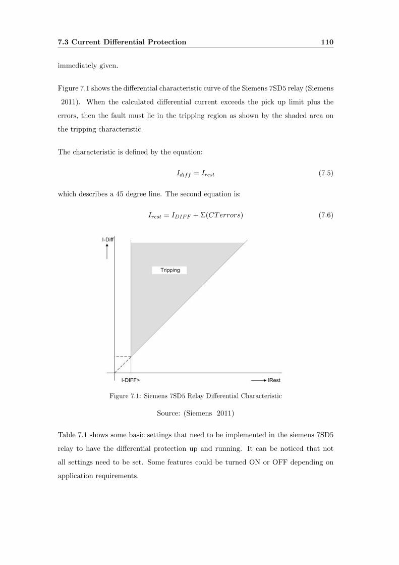
7.3 Current Differential Protection 110
immediately given.
Figure 7.1 shows the differential characteristic curve of the Siemens 7SD5 relay (Siemens
2011). When the calculated differential current exceeds the pick up limit plus the
errors, then the fault must lie in the tripping region as shown by the shaded area on
the tripping characteristic.
The characteristic is defined by the equation:
Idiff = Irest (7.5)
which describes a 45 degree line. The second equation is:
Irest = IDIFF + Σ(CTerrors) (7.6)
Figure 7.1: Siemens 7SD5 Relay Differential Characteristic
Source: (Siemens 2011)
Table 7.1 shows some basic settings that need to be implemented in the siemens 7SD5
relay to have the differential protection up and running. It can be noticed that not
all settings need to be set. Some features could be turned ON or OFF depending on
application requirements.
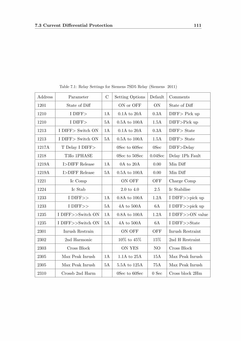
7.3 Current Differential Protection 111
Table 7.1: Relay Settings for Siemens 7SD5 Relay (Siemens 2011)
Address Parameter C Setting Options Default Comments
1201 State of Diff ON or OFF ON State of Diff
1210 I DIFF> 1A 0.1A to 20A 0.3A DIFF> Pick up
1210 I DIFF> 5A 0.5A to 100A 1.5A DIFF>Pick up
1213 I DIFF> Switch ON 1A 0.1A to 20A 0.3A DIFF> State
1213 I DIFF> Switch ON 5A 0.5A to 100A 1.5A DIFF> State
1217A T Delay I DIFF> 0Sec to 60Sec 0Sec DIFF>Delay
1218 T3Io 1PHASE 0Sec to 50Sec 0.04Sec Delay 1Ph Fault
1219A I>DIFF Release 1A 0A to 20A 0.00 Min Diff
1219A I>DIFF Release 5A 0.5A to 100A 0.00 Min Diff
1221 Ic Comp ON OFF OFF Charge Comp
1224 Ic Stab 2.0 to 4.0 2.5 Ic Stabilise
1233 I DIFF>> 1A 0.8A to 100A 1.2A I DIFF>>pick up
1233 I DIFF>> 5A 4A to 500A 6A I DIFF>>pick up
1235 I DIFF>>Switch ON 1A 0.8A to 100A 1.2A I DIFF>>ON value
1235 I DIFF>>Switch ON 5A 4A to 500A 6A I DIFF>>State
2301 Inrush Restrain ON OFF OFF Inrush Restraint
2302 2nd Harmonic 10% to 45% 15% 2nd H Restraint
2303 Cross Block ON YES NO Cross Block
2305 Max Peak Inrush 1A 1.1A to 25A 15A Max Peak Inrush
2305 Max Peak Inrush 5A 5.5A to 125A 75A Max Peak Inrush
2310 Crossb 2nd Harm 0Sec to 60Sec 0 Sec Cross block 2Hm
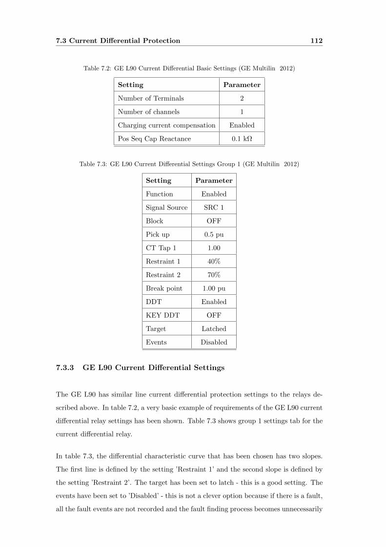
7.3 Current Differential Protection 112
Table 7.2: GE L90 Current Differential Basic Settings (GE Multilin 2012)
Setting Parameter
Number of Terminals 2
Number of channels 1
Charging current compensation Enabled
Pos Seq Cap Reactance 0.1 kΩ
Table 7.3: GE L90 Current Differential Settings Group 1 (GE Multilin 2012)
Setting Parameter
Function Enabled
Signal Source SRC 1
Block OFF
Pick up 0.5 pu
CT Tap 1 1.00
Restraint 1 40%
Restraint 2 70%
Break point 1.00 pu
DDT Enabled
KEY DDT OFF
Target Latched
Events Disabled
7.3.3 GE L90 Current Differential Settings
The GE L90 has similar line current differential protection settings to the relays de-
scribed above. In table 7.2, a very basic example of requirements of the GE L90 current
differential relay settings has been shown. Table 7.3 shows group 1 settings tab for the
current differential relay.
In table 7.3, the differential characteristic curve that has been chosen has two slopes.
The first line is defined by the setting ’Restraint 1’ and the second slope is defined by
the setting ’Restraint 2’. The target has been set to latch - this is a good setting. The
events have been set to ’Disabled’ - this is not a clever option because if there is a fault,
all the fault events are not recorded and the fault finding process becomes unnecessarily
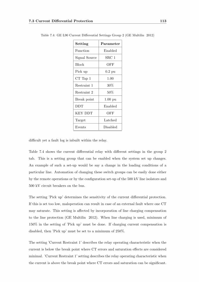
7.3 Current Differential Protection 113
Table 7.4: GE L90 Current Differential Settings Group 2 (GE Multilin 2012)
Setting Parameter
Function Enabled
Signal Source SRC 1
Block OFF
Pick up 0.2 pu
CT Tap 1 1.00
Restraint 1 30%
Restraint 2 50%
Break point 1.00 pu
DDT Enabled
KEY DDT OFF
Target Latched
Events Disabled
difficult yet a fault log is inbuilt within the relay.
Table 7.4 shows the current differential relay with different settings in the group 2
tab. This is a setting group that can be enabled when the system set up changes.
An example of such a set-up would be say a change in the loading conditions of a
particular line. Automation of changing these switch groups can be easily done either
by the remote operations or by the configuration set-up of the 500 kV line isolators and
500 kV circuit breakers on the bus.
The setting ’Pick up’ determines the sensitivity of the current differential protection.
If this is set too low, maloperation can result in case of an external fault where one CT
may saturate. This setting is affected by incorporation of line charging compensation
to the line protection (GE Multilin 2012). When line charging is used, minimum of
150% in the setting of ’Pick up’ must be done. If charging current compensation is
disabled, then ’Pick up’ must be set to a minimum of 250%.
The setting ’Current Restraint 1’ describes the relay operating characteristic when the
current is below the break point where CT errors and saturation effects are considered
minimal. ’Current Restraint 1’ setting describes the relay operating characteristic when
the current is above the break point where CT errors and saturation can be significant.
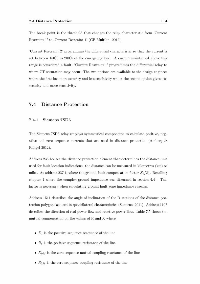
7.4 Distance Protection 114
The break point is the threshold that changes the relay characteristic from ’Current
Restraint 1’ to ’Current Restraint 1’ (GE Multilin 2012).
’Current Restraint 2’ programmes the differential characteristic so that the current is
set between 150% to 200% of the emergency load. A current maintained above this
range is considered a fault. ’Current Restraint 1’ programmes the differential relay to
where CT saturation may occur. The two options are available to the design engineer
where the first has more security and less sensitivity whilst the second option gives less
security and more sensitivity.
7.4 Distance Protection
7.4.1 Siemens 7SD5
The Siemens 7SD5 relay employs symmetrical components to calculate positive, neg-
ative and zero sequence currents that are used in distance protection (Amberg &
Rangel 2012).
Address 236 houses the distance protection element that determines the distance unit
used for fault location indications. the distance can be measured in kilometres (km) or
miles. At address 237 is where the ground fault compensation factor Z0/Z1. Recalling
chapter 4 where the complex ground impedance was discussed in section 4.4 . This
factor is necessary when calculating ground fault zone impedance reaches.
Address 1511 describes the angle of inclination of the R sections of the distance pro-
tection polygons as used in quadrilateral characteristics (Siemens 2011). Address 1107
describes the direction of real power flow and reactive power flow. Table 7.5 shows the
mutual compensation on the values of R and X where:
• X1 is the positive sequence reactance of the line
• R1 is the positive sequence resistance of the line
• X0M is the zero sequence mutual coupling reactance of the line
• R0M is the zero sequence coupling resistance of the line
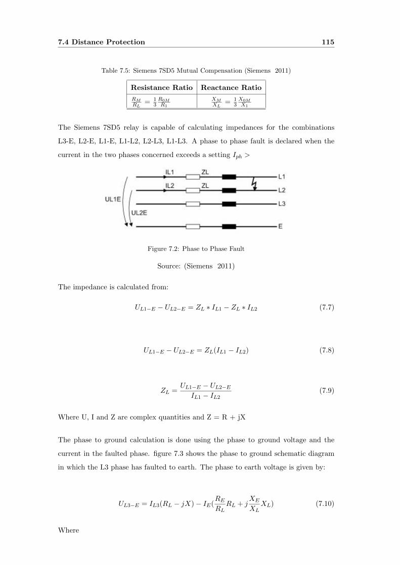
7.4 Distance Protection 115
Table 7.5: Siemens 7SD5 Mutual Compensation (Siemens 2011)
Resistance Ratio Reactance Ratio
RMRL
= 13R0MR1
XMXL
= 13X0MX1
The Siemens 7SD5 relay is capable of calculating impedances for the combinations
L3-E, L2-E, L1-E, L1-L2, L2-L3, L1-L3. A phase to phase fault is declared when the
current in the two phases concerned exceeds a setting Iph >
Figure 7.2: Phase to Phase Fault
Source: (Siemens 2011)
The impedance is calculated from:
UL1−E − UL2−E = ZL ∗ IL1 − ZL ∗ IL2 (7.7)
UL1−E − UL2−E = ZL(IL1 − IL2) (7.8)
ZL =UL1−E − UL2−E
IL1 − IL2(7.9)
Where U, I and Z are complex quantities and Z = R + jX
The phase to ground calculation is done using the phase to ground voltage and the
current in the faulted phase. figure 7.3 shows the phase to ground schematic diagram
in which the L3 phase has faulted to earth. The phase to earth voltage is given by:
UL3−E = IL3(RL − jX)− IE(RERL
RL + jXE
XLXL) (7.10)
Where
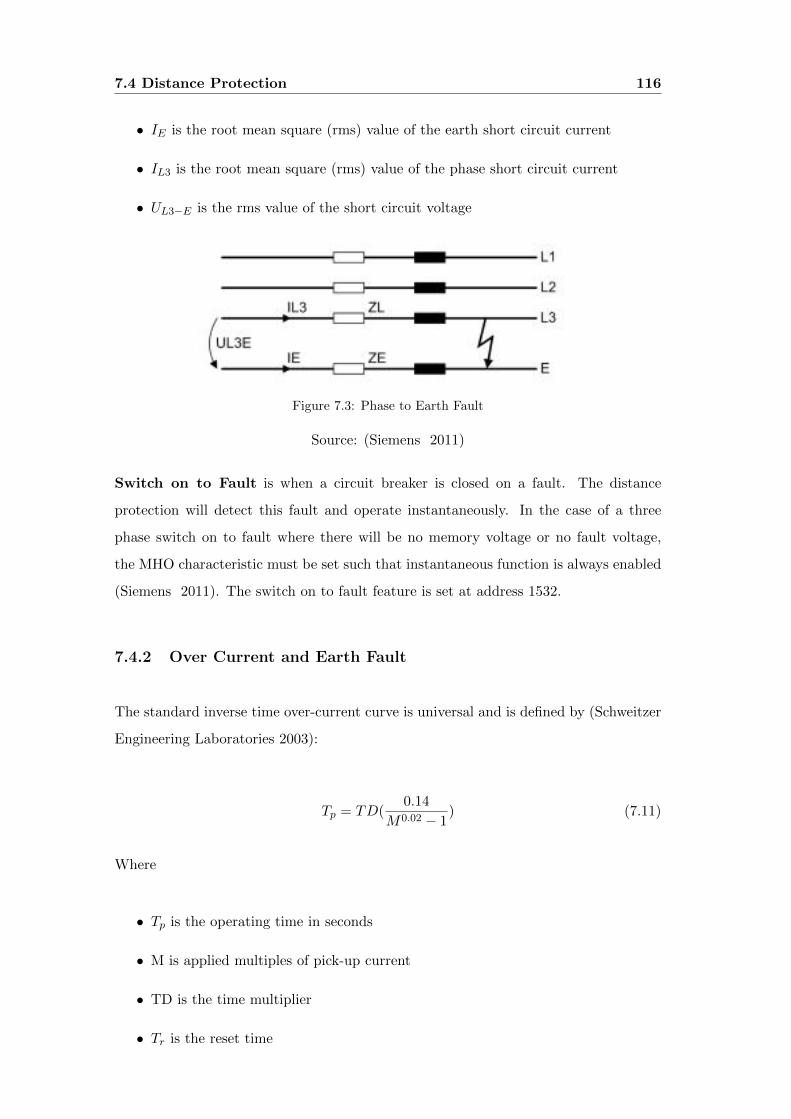
7.4 Distance Protection 116
• IE is the root mean square (rms) value of the earth short circuit current
• IL3 is the root mean square (rms) value of the phase short circuit current
• UL3−E is the rms value of the short circuit voltage
Figure 7.3: Phase to Earth Fault
Source: (Siemens 2011)
Switch on to Fault is when a circuit breaker is closed on a fault. The distance
protection will detect this fault and operate instantaneously. In the case of a three
phase switch on to fault where there will be no memory voltage or no fault voltage,
the MHO characteristic must be set such that instantaneous function is always enabled
(Siemens 2011). The switch on to fault feature is set at address 1532.
7.4.2 Over Current and Earth Fault
The standard inverse time over-current curve is universal and is defined by (Schweitzer
Engineering Laboratories 2003):
Tp = TD(0.14
M0.02 − 1) (7.11)
Where
• Tp is the operating time in seconds
• M is applied multiples of pick-up current
• TD is the time multiplier
• Tr is the reset time
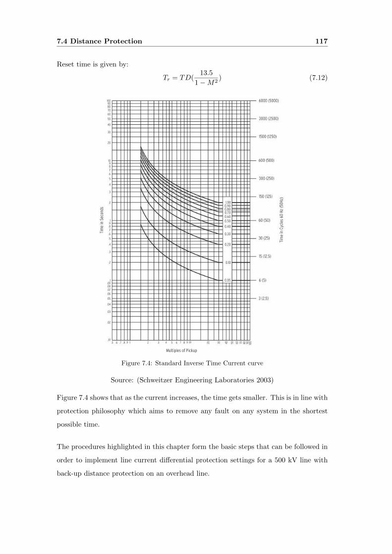
7.4 Distance Protection 117
Reset time is given by:
Tr = TD(13.5
1−M2) (7.12)
Figure 7.4: Standard Inverse Time Current curve
Source: (Schweitzer Engineering Laboratories 2003)
Figure 7.4 shows that as the current increases, the time gets smaller. This is in line with
protection philosophy which aims to remove any fault on any system in the shortest
possible time.
The procedures highlighted in this chapter form the basic steps that can be followed in
order to implement line current differential protection settings for a 500 kV line with
back-up distance protection on an overhead line.
7.5 Chapter Summary 118
7.5 Chapter Summary
This chapter has looked at the Aspen software that is used to manage and store relay
settings and lines information.
Basic steps needed to configure line current differential settings for SEL 31L, GE L90
and Siemens 7SD5 relays have been shown.
Basic steps needed to configure distance protection settings for SEL 31L, GE L90 and
Siemens 7SD5 relays have been shown.
Chapter 8
500 kV Circuit Breaker
8.1 Chapter Overview
This chapter looks at various aspects of a typical 500 kV circuit breaker. A look at an
sulphur hexaflouride SF6 circuit breaker is done. Tests that are done on circuit breakers
are discussed. Timing and arc quenching mechanisms are covered in this chapter.
8.2 Circuit Breaker Timing
As the 500 kV CB (circuit breaker) is the ultimate item in isolating a fault on a 500
kV line, it is important that time is allocated to the discussion the CB plays in a line
protection sequence.
The 500 kV CB isolates the faulty section of the 500 kV line and as such it carries the
duty of interrupting high fault currents. It is important to know the time it takes for a
circuit breaker to operate once given a command to open or close. It is very important
that a CB must operate very fast in order to clear any fault to preserve system stability
(Grainger & Stevenson 1994) . On a 500 kV line, there is need for a CB to perform a
sequence such as o-c-o (open close open) or c-o ( close open) in a reasonably very short
possible time.
When a CB opens, the open contacts become voltage dividers. If the contacts open
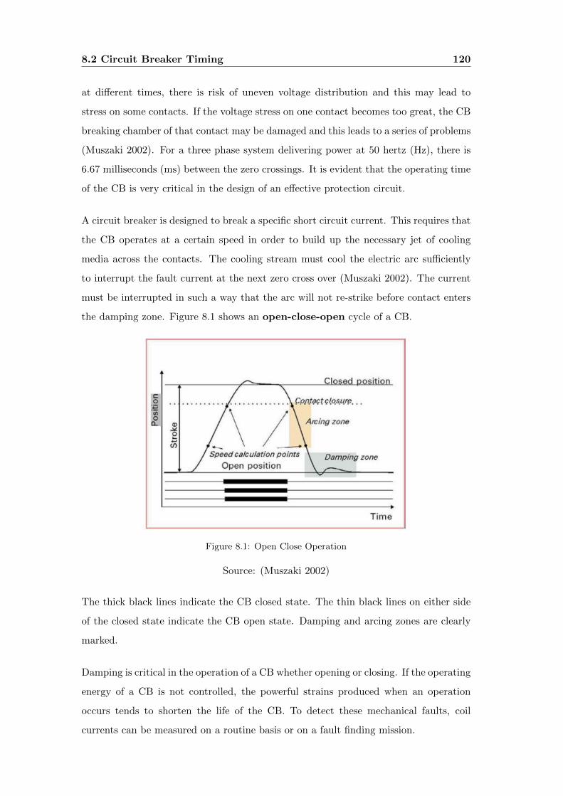
8.2 Circuit Breaker Timing 120
at different times, there is risk of uneven voltage distribution and this may lead to
stress on some contacts. If the voltage stress on one contact becomes too great, the CB
breaking chamber of that contact may be damaged and this leads to a series of problems
(Muszaki 2002). For a three phase system delivering power at 50 hertz (Hz), there is
6.67 milliseconds (ms) between the zero crossings. It is evident that the operating time
of the CB is very critical in the design of an effective protection circuit.
A circuit breaker is designed to break a specific short circuit current. This requires that
the CB operates at a certain speed in order to build up the necessary jet of cooling
media across the contacts. The cooling stream must cool the electric arc sufficiently
to interrupt the fault current at the next zero cross over (Muszaki 2002). The current
must be interrupted in such a way that the arc will not re-strike before contact enters
the damping zone. Figure 8.1 shows an open-close-open cycle of a CB.
Figure 8.1: Open Close Operation
Source: (Muszaki 2002)
The thick black lines indicate the CB closed state. The thin black lines on either side
of the closed state indicate the CB open state. Damping and arcing zones are clearly
marked.
Damping is critical in the operation of a CB whether opening or closing. If the operating
energy of a CB is not controlled, the powerful strains produced when an operation
occurs tends to shorten the life of the CB. To detect these mechanical faults, coil
currents can be measured on a routine basis or on a fault finding mission.
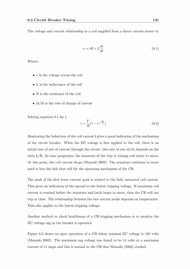
8.2 Circuit Breaker Timing 121
The voltage and current relationship in a coil supplied from a direct current source is:
v = iR+ Ldi
dt(8.1)
Where:
• v is the voltage across the coil
• L is the inductance of the coil
• R is the resistance of the coil
• di/dt is the rate of change of current
Solving equation 8.1 for i:
i =V
R(1− e−
RtL ) (8.2)
Monitoring the behaviour of the coil current i gives a good indication of the mechanism
of the circuit breaker. When the DC voltage is first applied to the coil, there is an
initial rate of rise of current through the circuit, this rate of rise di/dt depends on the
ratio L/R. As time progresses, the armature of the trip or closing coil starts to move.
At this point, the coil current drops (Muszaki 2002). The armature continues to move
until it hits the lath that will hit the operating mechanism of the CB.
The peak of the first lower current peak is related to the fully saturated coil current.
This gives an indication of the spread to the lowest tripping voltage. If maximum coil
current is reached before the armature and latch begin to move, then the CB will not
trip or close. The relationship between the two current peaks depends on temperature.
Thia also applies to the lowest tripping voltage.
Another method to check healthiness of a CB tripping mechanism is to monitor the
DC voltage sag as the breaker is operated.
Figure 8.2 shows an open operation of a CB whose nominal DC voltage is 128 volts
(Muszaki 2002). The maximum sag voltage was found to be 14 volts at a maximum
current of 11 amps and this is normal to the CB that Muszaki (2002) studied.
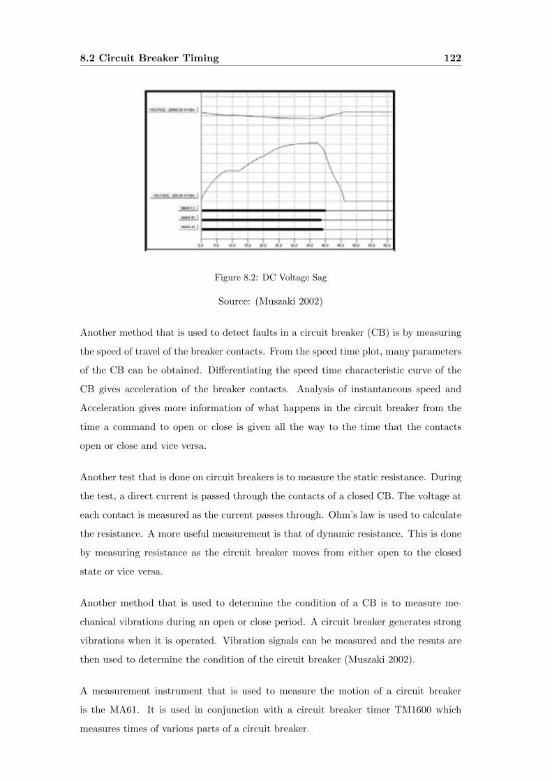
8.2 Circuit Breaker Timing 122
Figure 8.2: DC Voltage Sag
Source: (Muszaki 2002)
Another method that is used to detect faults in a circuit breaker (CB) is by measuring
the speed of travel of the breaker contacts. From the speed time plot, many parameters
of the CB can be obtained. Differentiating the speed time characteristic curve of the
CB gives acceleration of the breaker contacts. Analysis of instantaneous speed and
Acceleration gives more information of what happens in the circuit breaker from the
time a command to open or close is given all the way to the time that the contacts
open or close and vice versa.
Another test that is done on circuit breakers is to measure the static resistance. During
the test, a direct current is passed through the contacts of a closed CB. The voltage at
each contact is measured as the current passes through. Ohm’s law is used to calculate
the resistance. A more useful measurement is that of dynamic resistance. This is done
by measuring resistance as the circuit breaker moves from either open to the closed
state or vice versa.
Another method that is used to determine the condition of a CB is to measure me-
chanical vibrations during an open or close period. A circuit breaker generates strong
vibrations when it is operated. Vibration signals can be measured and the resuts are
then used to determine the condition of the circuit breaker (Muszaki 2002).
A measurement instrument that is used to measure the motion of a circuit breaker
is the MA61. It is used in conjunction with a circuit breaker timer TM1600 which
measures times of various parts of a circuit breaker.
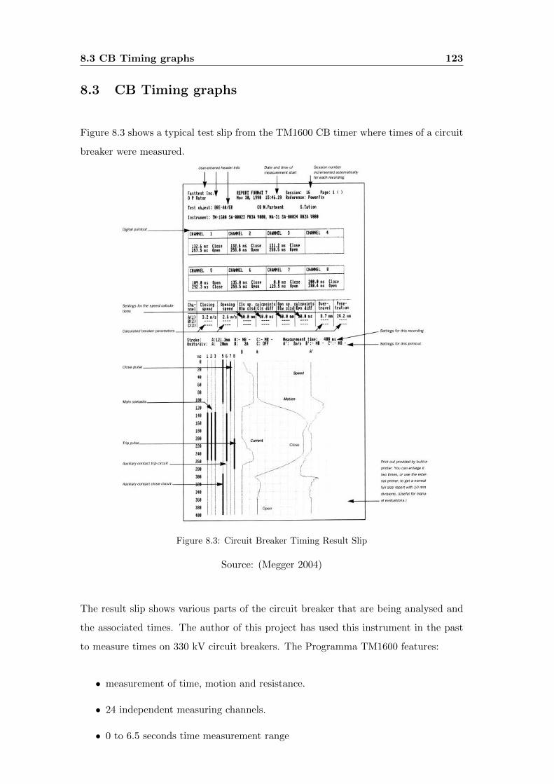
8.3 CB Timing graphs 123
8.3 CB Timing graphs
Figure 8.3 shows a typical test slip from the TM1600 CB timer where times of a circuit
breaker were measured.
Figure 8.3: Circuit Breaker Timing Result Slip
Source: (Megger 2004)
The result slip shows various parts of the circuit breaker that are being analysed and
the associated times. The author of this project has used this instrument in the past
to measure times on 330 kV circuit breakers. The Programma TM1600 features:
• measurement of time, motion and resistance.
• 24 independent measuring channels.
• 0 to 6.5 seconds time measurement range
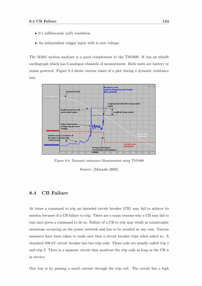
8.4 CB Failure 124
• 0.1 milliseconds (mS) resolution
• An independent trigger input with is own voltage.
The MA61 motion analyser is a good complement to the TM1600. It has an inbuilt
oscillograph which has 6 analogue channels of measurement. Both units are battery or
mains powered. Figure 8.4 shows various times of a plot during a dynamic resistance
test.
Figure 8.4: Dynamic resistance Measurement using TM1800
Source: (Muszaki 2002)
8.4 CB Failure
At times a command to trip an intended circuit breaker (CB) may fail to achieve its
mission because of a CB failure to trip. There are a many reasons why a CB may fail to
trip once given a command to do so. Failure of a CB to trip may result in catastrophic
situations occurring on the power network and has to be avoided at any cost. Various
measures have been taken to make sure that a circuit breaker trips when asked to. A
standard 500 kV circuit breaker has two trip coils. These coils are usually called trip 1
and trip 2. There is a separate circuit that monitors the trip coils as long as the CB is
in service.
One way is by passing a small current through the trip coil. The circuit has a high
8.4 CB Failure 125
value of resistance so that the flowing current does not cause the coil to operate and
trips the CB. The small current passed through the trip coil is typically 1.5 mA. This
current flows whether the CB is on local or remote selection. If the 1.5 mA current
stops flowing, an alarm is issued and the circuit must be checked for loss of DC supply
or the trip circuit is faulty or the trip coil itself is faulty.
One such relay is the Asea Brown Boveri (ABB) SPER 1C1 relay. There are different
design voltages of this relay. The design voltages are 48v, 60v, 110v, and 220v. A
different version to the SPER 1C1 relay is the SPER 1C2 relay whose DC voltages are
30v and 48v respectively and the current flow is 5 mA (ABB 2013). The resistors that
go with the SPER 1C1 relay are:
• 1.2 kΩ 5 watt resistor for the 45v dc relay
• 5.6 kΩ 5 watt resistor for the 60v dc relay
• 22 kΩ 5 watt resistor for the 110v dc relay
• 33 kΩ 5 watt resistor for the 220v dc relay
The ABB SPER 1C2 relay has:
• 380 Ω 5 watt resistor for the 30v dc relay
• 2.2 kΩ 5 watt resistor for the 48v dc relay
Another way to prevent circuit breaker failure is to monitor the availability of tripping
energy. In some circuit breakers there are springs that are compressed as the breaker
is closed. This means that there is stored energy ready to be released when wanted.
Monitoring that the springs are charged is a good way to guarantee a trip. There is
an alarm contact that is linked to the spring driven mechanism that closes when the
tripping spring is discharged. The author has worked on 33 kV circuit breakers with
this feature.
Coupled with the tripping springs is the springs charging motor. At times it is necessary
to monitor the spring charging motor as well. An unusual increase in the motor current
indicates some fault on the mechanism. An unusual sound coming from the charging
springs is another way to monitor the circuit breaker mechanism. At times audible
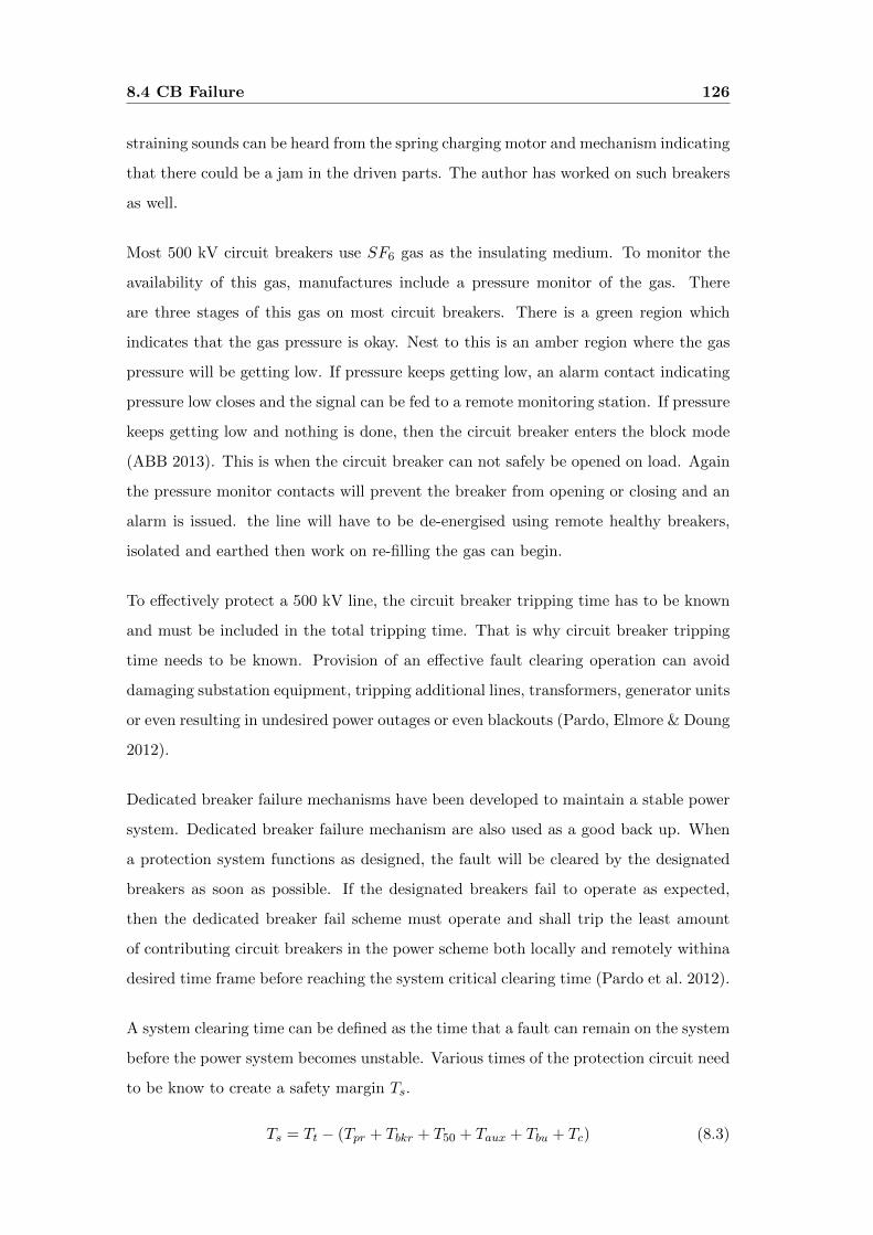
8.4 CB Failure 126
straining sounds can be heard from the spring charging motor and mechanism indicating
that there could be a jam in the driven parts. The author has worked on such breakers
as well.
Most 500 kV circuit breakers use SF6 gas as the insulating medium. To monitor the
availability of this gas, manufactures include a pressure monitor of the gas. There
are three stages of this gas on most circuit breakers. There is a green region which
indicates that the gas pressure is okay. Nest to this is an amber region where the gas
pressure will be getting low. If pressure keeps getting low, an alarm contact indicating
pressure low closes and the signal can be fed to a remote monitoring station. If pressure
keeps getting low and nothing is done, then the circuit breaker enters the block mode
(ABB 2013). This is when the circuit breaker can not safely be opened on load. Again
the pressure monitor contacts will prevent the breaker from opening or closing and an
alarm is issued. the line will have to be de-energised using remote healthy breakers,
isolated and earthed then work on re-filling the gas can begin.
To effectively protect a 500 kV line, the circuit breaker tripping time has to be known
and must be included in the total tripping time. That is why circuit breaker tripping
time needs to be known. Provision of an effective fault clearing operation can avoid
damaging substation equipment, tripping additional lines, transformers, generator units
or even resulting in undesired power outages or even blackouts (Pardo, Elmore & Doung
2012).
Dedicated breaker failure mechanisms have been developed to maintain a stable power
system. Dedicated breaker failure mechanism are also used as a good back up. When
a protection system functions as designed, the fault will be cleared by the designated
breakers as soon as possible. If the designated breakers fail to operate as expected,
then the dedicated breaker fail scheme must operate and shall trip the least amount
of contributing circuit breakers in the power scheme both locally and remotely withina
desired time frame before reaching the system critical clearing time (Pardo et al. 2012).
A system clearing time can be defined as the time that a fault can remain on the system
before the power system becomes unstable. Various times of the protection circuit need
to be know to create a safety margin Ts.
Ts = Tt − (Tpr + Tbkr + T50 + Taux + Tbu + Tc) (8.3)
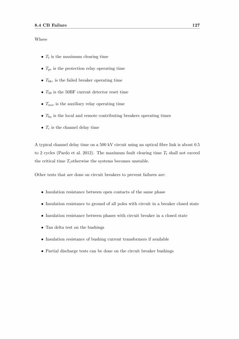
8.4 CB Failure 127
Where
• Tt is the maximum clearing time
• Tpr is the protection relay operating time
• Tbkr is the failed breaker operating time
• T50 is the 50BF current detector reset time
• Taux is the auxiliary relay operating time
• Tbu is the local and remote contributing breakers operating times
• Tc is the channel delay time
A typical channel delay time on a 500 kV circuit using an optical fibre link is about 0.5
to 2 cycles (Pardo et al. 2012). The maximum fault clearing time Tt shall not exceed
the critical time Tcotherwise the systems becomes unstable.
Other tests that are done on circuit breakers to prevent failures are:
• Insulation resistance between open contacts of the same phase
• Insulation resistance to ground of all poles with circuit in a breaker closed state
• Insulation resistance between phases with circuit breaker in a closed state
• Tan delta test on the bushings
• Insulation resistance of bushing current transformers if available
• Partial discharge tests can be done on the circuit breaker bushings
8.5 Chapter Summary 128
8.5 Chapter Summary
This chapter has covered work on high voltage circuit breakers. It has been shown that
it is important to have a good functioning circuit breaker on a 500 kV system in order
to maintain a stable power grid.
Efforts to have a good working circuit breaker involve good maintenance cycles and
periodic checks. Condition monitoring of the circuit breaker is also necessary. These
checks could be contact resistance test, dynamic resistance test, spring charging motor
checks and SF6 gas monitoring.
Other routine checks have been shown to include insulation resistance test on various
paths of the circuit breaker poles. Insulation resistance on the current transformers
need to be done if the circuit breaker has in-built current transformers. Tan delta tests
can also be done on the bushings. If there is a need, partial discharge measurement
can be done on the bushings.
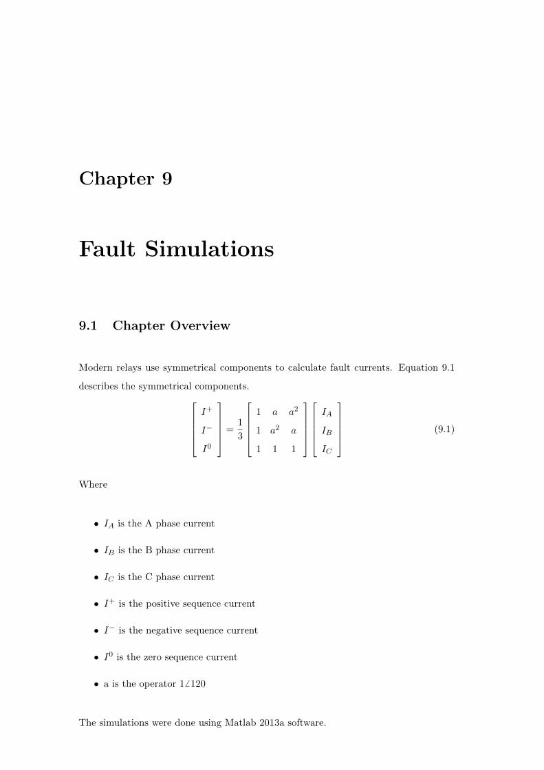
Chapter 9
Fault Simulations
9.1 Chapter Overview
Modern relays use symmetrical components to calculate fault currents. Equation 9.1
describes the symmetrical components.I+
I−
I0
=1
3
1 a a2
1 a2 a
1 1 1
IA
IB
IC
(9.1)
Where
• IA is the A phase current
• IB is the B phase current
• IC is the C phase current
• I+ is the positive sequence current
• I− is the negative sequence current
• I0 is the zero sequence current
• a is the operator 1 6 120
The simulations were done using Matlab 2013a software.
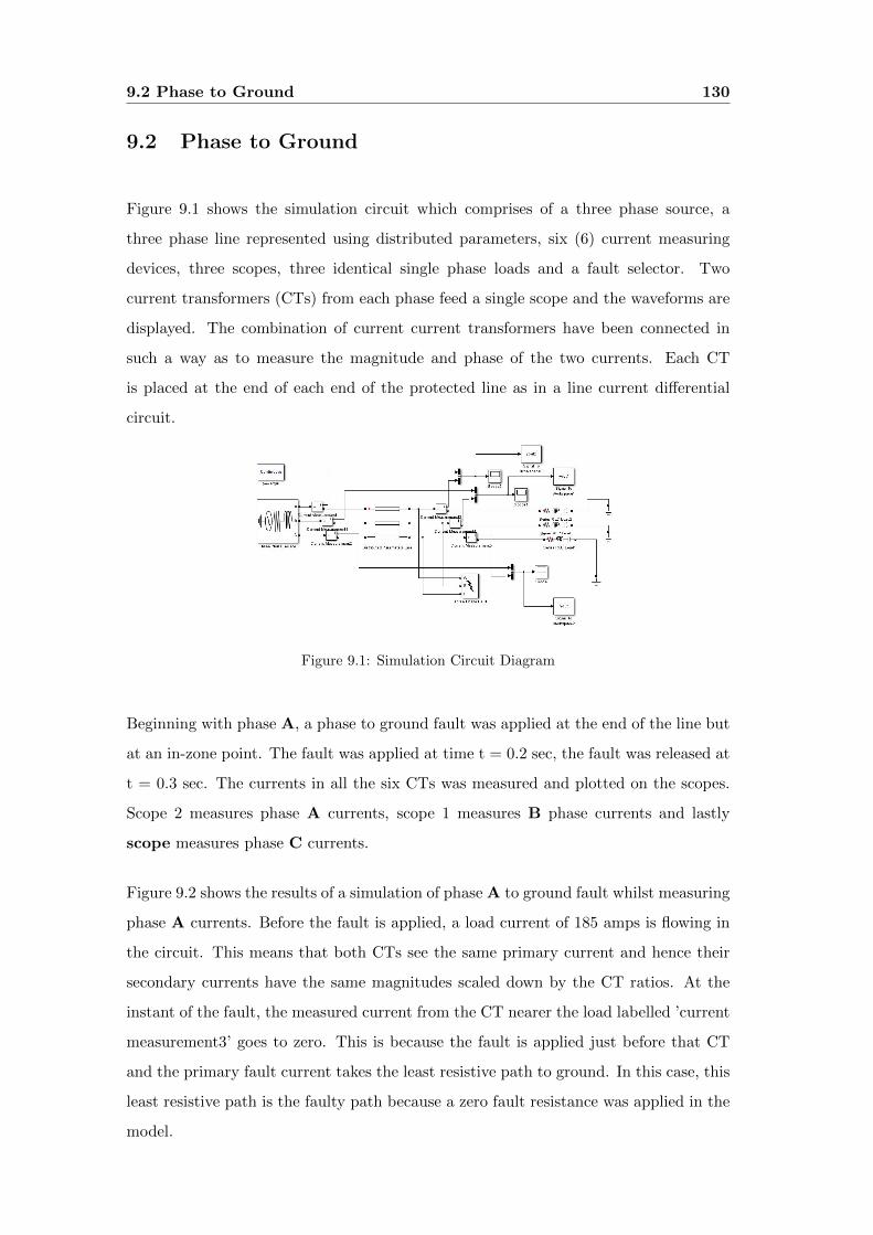
9.2 Phase to Ground 130
9.2 Phase to Ground
Figure 9.1 shows the simulation circuit which comprises of a three phase source, a
three phase line represented using distributed parameters, six (6) current measuring
devices, three scopes, three identical single phase loads and a fault selector. Two
current transformers (CTs) from each phase feed a single scope and the waveforms are
displayed. The combination of current current transformers have been connected in
such a way as to measure the magnitude and phase of the two currents. Each CT
is placed at the end of each end of the protected line as in a line current differential
circuit.
Figure 9.1: Simulation Circuit Diagram
Beginning with phase A, a phase to ground fault was applied at the end of the line but
at an in-zone point. The fault was applied at time t = 0.2 sec, the fault was released at
t = 0.3 sec. The currents in all the six CTs was measured and plotted on the scopes.
Scope 2 measures phase A currents, scope 1 measures B phase currents and lastly
scope measures phase C currents.
Figure 9.2 shows the results of a simulation of phase A to ground fault whilst measuring
phase A currents. Before the fault is applied, a load current of 185 amps is flowing in
the circuit. This means that both CTs see the same primary current and hence their
secondary currents have the same magnitudes scaled down by the CT ratios. At the
instant of the fault, the measured current from the CT nearer the load labelled ’current
measurement3’ goes to zero. This is because the fault is applied just before that CT
and the primary fault current takes the least resistive path to ground. In this case, this
least resistive path is the faulty path because a zero fault resistance was applied in the
model.
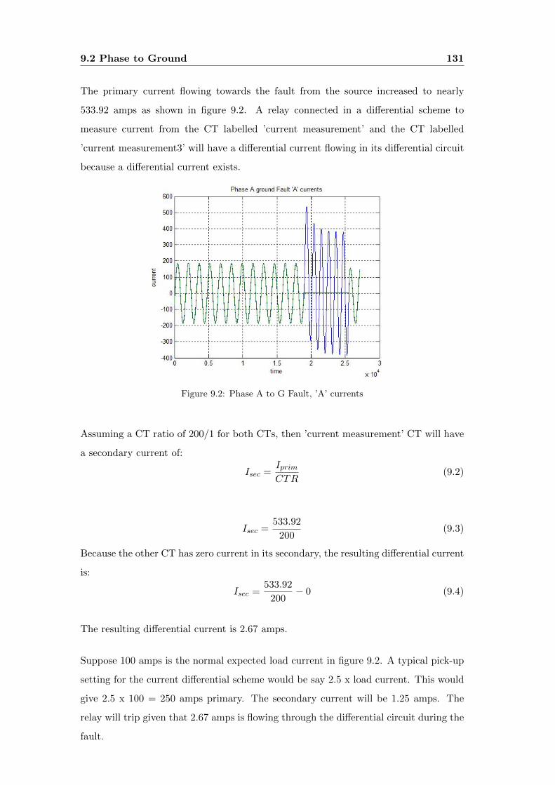
9.2 Phase to Ground 131
The primary current flowing towards the fault from the source increased to nearly
533.92 amps as shown in figure 9.2. A relay connected in a differential scheme to
measure current from the CT labelled ’current measurement’ and the CT labelled
’current measurement3’ will have a differential current flowing in its differential circuit
because a differential current exists.
Figure 9.2: Phase A to G Fault, ’A’ currents
Assuming a CT ratio of 200/1 for both CTs, then ’current measurement’ CT will have
a secondary current of:
Isec =IprimCTR
(9.2)
Isec =533.92
200(9.3)
Because the other CT has zero current in its secondary, the resulting differential current
is:
Isec =533.92
200− 0 (9.4)
The resulting differential current is 2.67 amps.
Suppose 100 amps is the normal expected load current in figure 9.2. A typical pick-up
setting for the current differential scheme would be say 2.5 x load current. This would
give 2.5 x 100 = 250 amps primary. The secondary current will be 1.25 amps. The
relay will trip given that 2.67 amps is flowing through the differential circuit during the
fault.
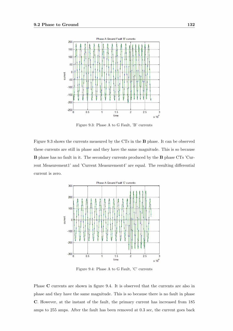
9.2 Phase to Ground 132
Figure 9.3: Phase A to G Fault, ’B’ currents
Figure 9.3 shows the currents measured by the CTs in the B phase. It can be observed
these currents are still in phase and they have the same magnitude. This is so because
B phase has no fault in it. The secondary currents produced by the B phase CTs ’Cur-
rent Measurement1’ and ’Current Measurement4’ are equal. The resulting differential
current is zero.
Figure 9.4: Phase A to G Fault, ’C’ currents
Phase C currents are shown in figure 9.4. It is observed that the currents are also in
phase and they have the same magnitude. This is so because there is no fault in phase
C. However, at the instant of the fault, the primary current has increased from 185
amps to 255 amps. After the fault has been removed at 0.3 sec, the current goes back
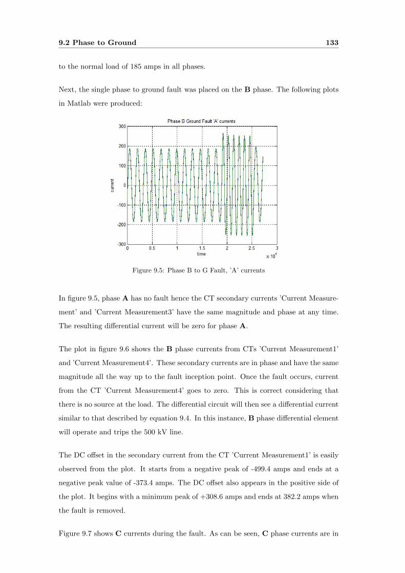
9.2 Phase to Ground 133
to the normal load of 185 amps in all phases.
Next, the single phase to ground fault was placed on the B phase. The following plots
in Matlab were produced:
Figure 9.5: Phase B to G Fault, ’A’ currents
In figure 9.5, phase A has no fault hence the CT secondary currents ’Current Measure-
ment’ and ’Current Measurement3’ have the same magnitude and phase at any time.
The resulting differential current will be zero for phase A.
The plot in figure 9.6 shows the B phase currents from CTs ’Current Measurement1’
and ’Current Measurement4’. These secondary currents are in phase and have the same
magnitude all the way up to the fault inception point. Once the fault occurs, current
from the CT ’Current Measurement4’ goes to zero. This is correct considering that
there is no source at the load. The differential circuit will then see a differential current
similar to that described by equation 9.4. In this instance, B phase differential element
will operate and trips the 500 kV line.
The DC offset in the secondary current from the CT ’Current Measurement1’ is easily
observed from the plot. It starts from a negative peak of -499.4 amps and ends at a
negative peak value of -373.4 amps. The DC offset also appears in the positive side of
the plot. It begins with a minimum peak of +308.6 amps and ends at 382.2 amps when
the fault is removed.
Figure 9.7 shows C currents during the fault. As can be seen, C phase currents are in
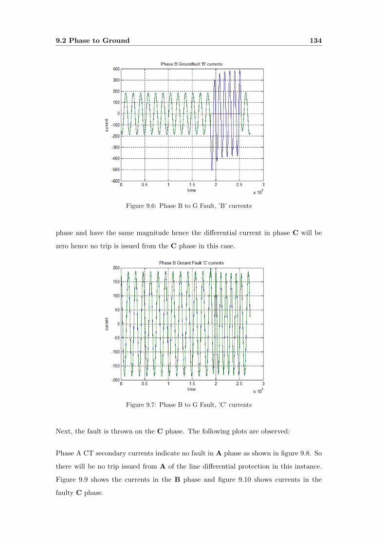
9.2 Phase to Ground 134
Figure 9.6: Phase B to G Fault, ’B’ currents
phase and have the same magnitude hence the differential current in phase C will be
zero hence no trip is issued from the C phase in this case.
Figure 9.7: Phase B to G Fault, ’C’ currents
Next, the fault is thrown on the C phase. The following plots are observed:
Phase A CT secondary currents indicate no fault in A phase as shown in figure 9.8. So
there will be no trip issued from A of the line differential protection in this instance.
Figure 9.9 shows the currents in the B phase and figure 9.10 shows currents in the
faulty C phase.
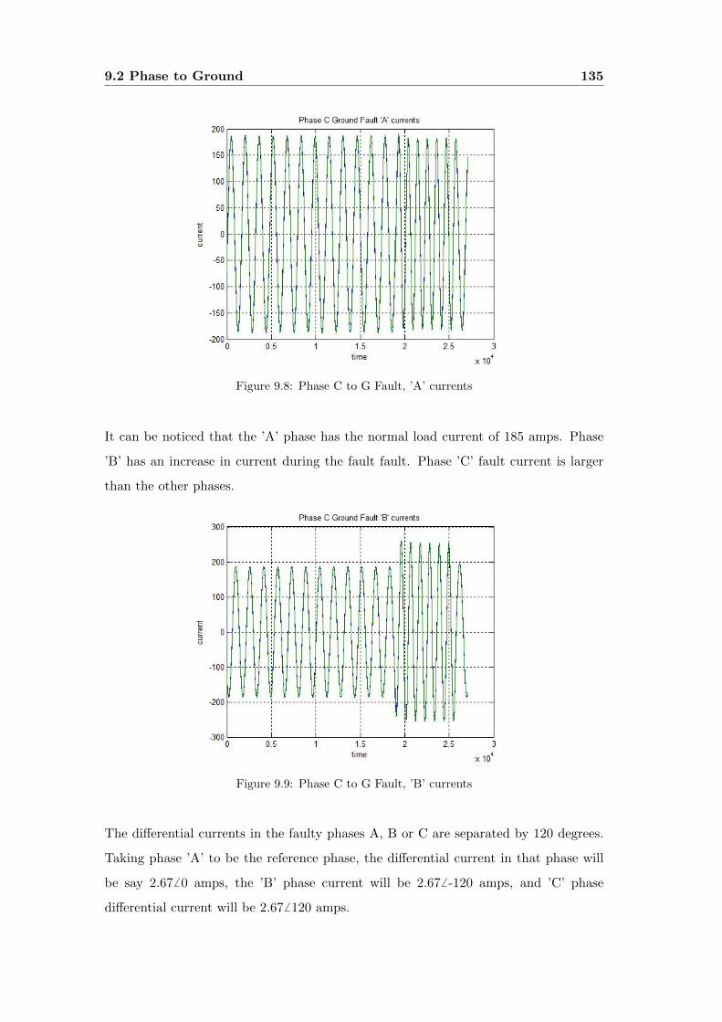
9.2 Phase to Ground 135
Figure 9.8: Phase C to G Fault, ’A’ currents
It can be noticed that the ’A’ phase has the normal load current of 185 amps. Phase
’B’ has an increase in current during the fault fault. Phase ’C’ fault current is larger
than the other phases.
Figure 9.9: Phase C to G Fault, ’B’ currents
The differential currents in the faulty phases A, B or C are separated by 120 degrees.
Taking phase ’A’ to be the reference phase, the differential current in that phase will
be say 2.67 6 0 amps, the ’B’ phase current will be 2.67 6 -120 amps, and ’C’ phase
differential current will be 2.67 6 120 amps.
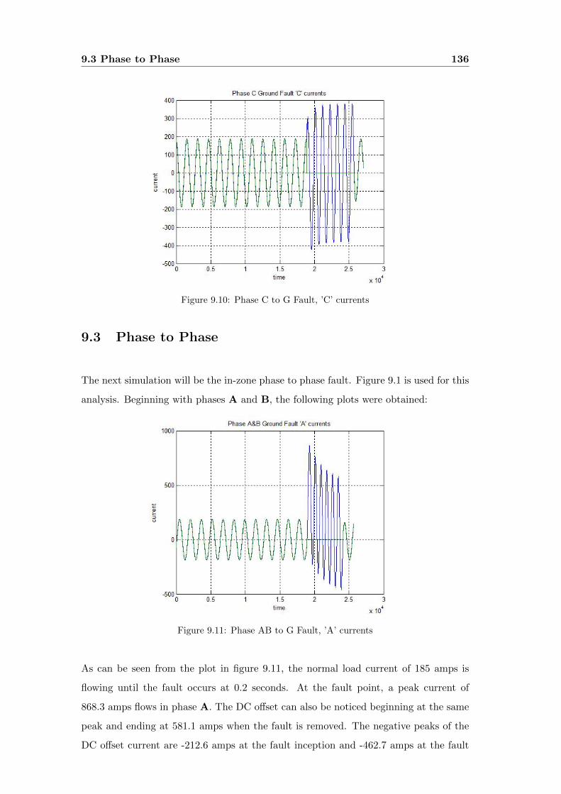
9.3 Phase to Phase 136
Figure 9.10: Phase C to G Fault, ’C’ currents
9.3 Phase to Phase
The next simulation will be the in-zone phase to phase fault. Figure 9.1 is used for this
analysis. Beginning with phases A and B, the following plots were obtained:
Figure 9.11: Phase AB to G Fault, ’A’ currents
As can be seen from the plot in figure 9.11, the normal load current of 185 amps is
flowing until the fault occurs at 0.2 seconds. At the fault point, a peak current of
868.3 amps flows in phase A. The DC offset can also be noticed beginning at the same
peak and ending at 581.1 amps when the fault is removed. The negative peaks of the
DC offset current are -212.6 amps at the fault inception and -462.7 amps at the fault
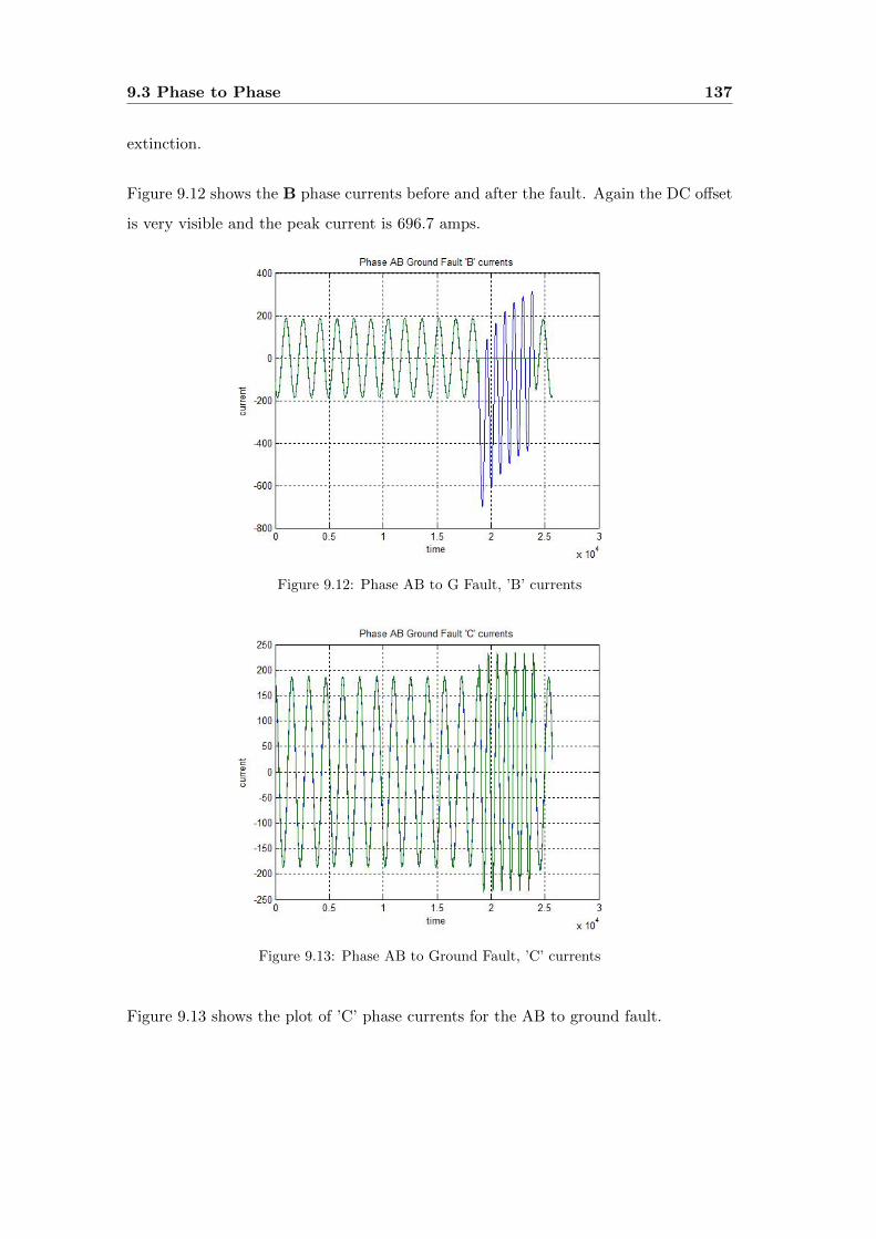
9.3 Phase to Phase 137
extinction.
Figure 9.12 shows the B phase currents before and after the fault. Again the DC offset
is very visible and the peak current is 696.7 amps.
Figure 9.12: Phase AB to G Fault, ’B’ currents
Figure 9.13: Phase AB to Ground Fault, ’C’ currents
Figure 9.13 shows the plot of ’C’ phase currents for the AB to ground fault.
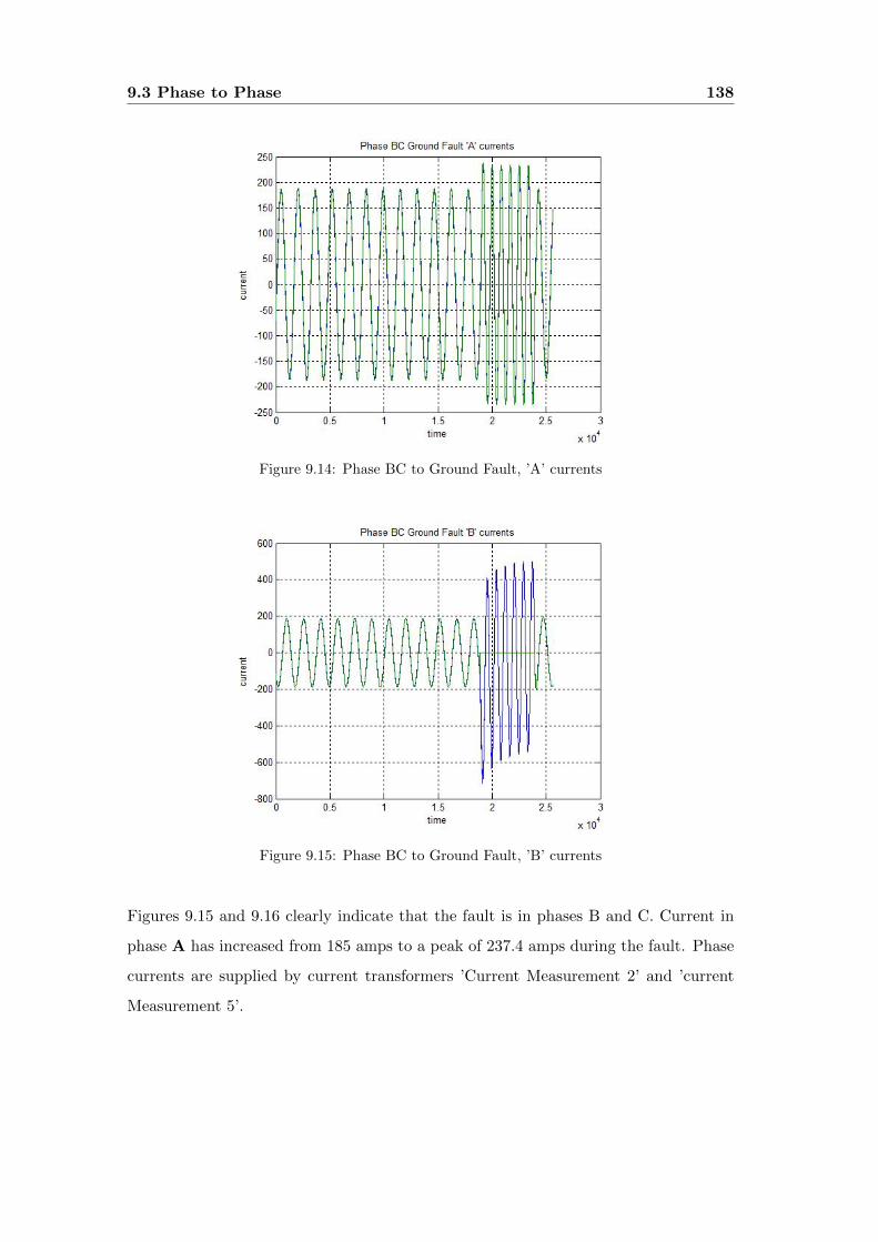
9.3 Phase to Phase 138
Figure 9.14: Phase BC to Ground Fault, ’A’ currents
Figure 9.15: Phase BC to Ground Fault, ’B’ currents
Figures 9.15 and 9.16 clearly indicate that the fault is in phases B and C. Current in
phase A has increased from 185 amps to a peak of 237.4 amps during the fault. Phase
currents are supplied by current transformers ’Current Measurement 2’ and ’current
Measurement 5’.
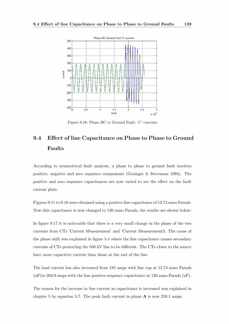
9.4 Effect of line Capacitance on Phase to Phase to Ground Faults 139
Figure 9.16: Phase BC to Ground Fault, ’C’ currents
9.4 Effect of line Capacitance on Phase to Phase to Ground
Faults
According to symmetrical fault analysis, a phase to phase to ground fault involves
positive, negative and zero sequence components (Grainger & Stevenson 1994). The
positive and zero sequence capacitances are now varied to see the effect on the fault
current plots.
Figures 9.11 to 9.16 were obtained using a positive line capacitance of 12.74 nano Farads.
Now this capacitance is now changed to 120 nano Farads, the results are shown below:
In figure 9.17 it is noticeable that there is a very small change in the phase of the two
currents from CTs ’Current Measurement’ and ’Current Measurement3. The cause of
the phase shift was explained in figure 5.4 where the line capacitance causes secondary
currents of CTs protecting the 500 kV line to be different. The CTs closer to the source
have more capacitive current than those at the end of the line.
The load current has also increased from 185 amps with line cap at 12.74 nano Farads
(nF)to 203.9 amps with the line positive sequence capacitance at 120 nano Farads (nF).
The reason for the increase in line current as capacitance is increased was explained in
chapter 5 by equation 5.7. The peak fault current in phase A is now 250.1 amps.
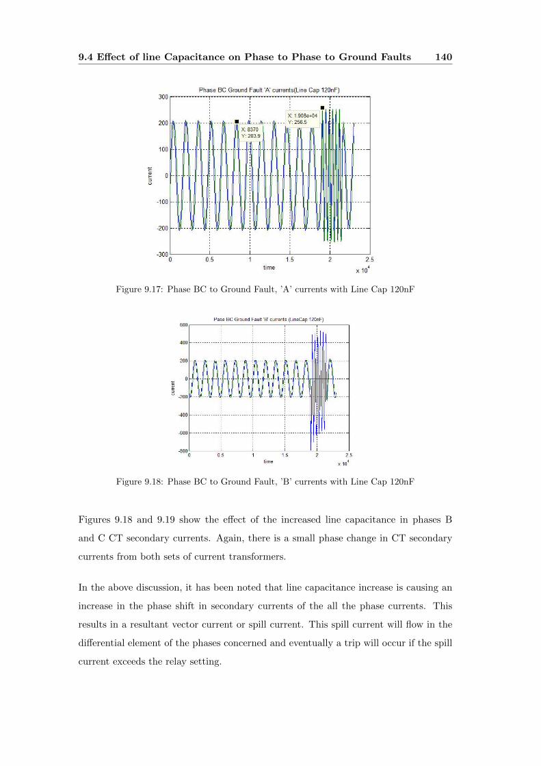
9.4 Effect of line Capacitance on Phase to Phase to Ground Faults 140
Figure 9.17: Phase BC to Ground Fault, ’A’ currents with Line Cap 120nF
Figure 9.18: Phase BC to Ground Fault, ’B’ currents with Line Cap 120nF
Figures 9.18 and 9.19 show the effect of the increased line capacitance in phases B
and C CT secondary currents. Again, there is a small phase change in CT secondary
currents from both sets of current transformers.
In the above discussion, it has been noted that line capacitance increase is causing an
increase in the phase shift in secondary currents of the all the phase currents. This
results in a resultant vector current or spill current. This spill current will flow in the
differential element of the phases concerned and eventually a trip will occur if the spill
current exceeds the relay setting.
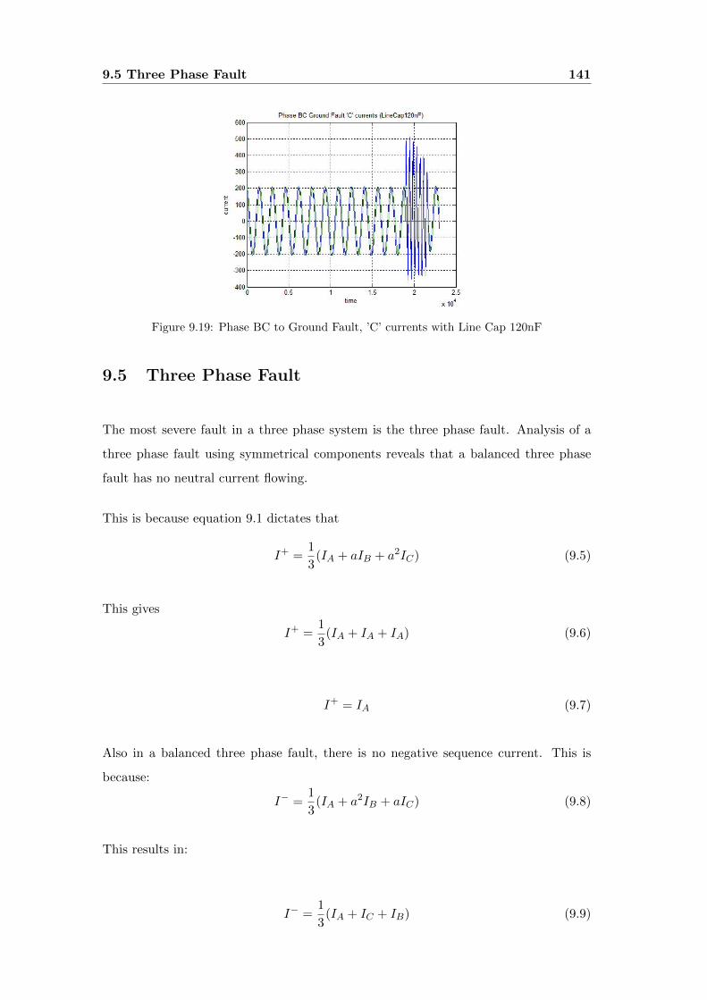
9.5 Three Phase Fault 141
Figure 9.19: Phase BC to Ground Fault, ’C’ currents with Line Cap 120nF
9.5 Three Phase Fault
The most severe fault in a three phase system is the three phase fault. Analysis of a
three phase fault using symmetrical components reveals that a balanced three phase
fault has no neutral current flowing.
This is because equation 9.1 dictates that
I+ =1
3(IA + aIB + a2IC) (9.5)
This gives
I+ =1
3(IA + IA + IA) (9.6)
I+ = IA (9.7)
Also in a balanced three phase fault, there is no negative sequence current. This is
because:
I− =1
3(IA + a2IB + aIC) (9.8)
This results in:
I− =1
3(IA + IC + IB) (9.9)
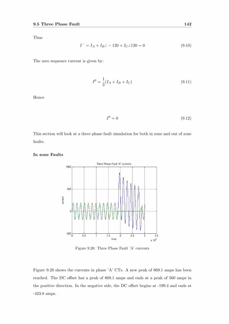
9.5 Three Phase Fault 142
Thus
I− = IA + IB 6 − 120 + IC 6 120 = 0 (9.10)
The zero sequence current is given by:
I0 =1
3(IA + IB + IC) (9.11)
Hence
I0 = 0 (9.12)
This section will look at a three phase fault simulation for both in zone and out of zone
faults.
In zone Faults
Figure 9.20: Three Phase Fault ’A’ currents
Figure 9.20 shows the currents in phase ’A’ CTs. A new peak of 869.1 amps has been
reached. The DC offset has a peak of 869.1 amps and ends at a peak of 560 amps in
the positive direction. In the negative side, the DC offset begins at -199.4 and ends at
-423.8 amps.
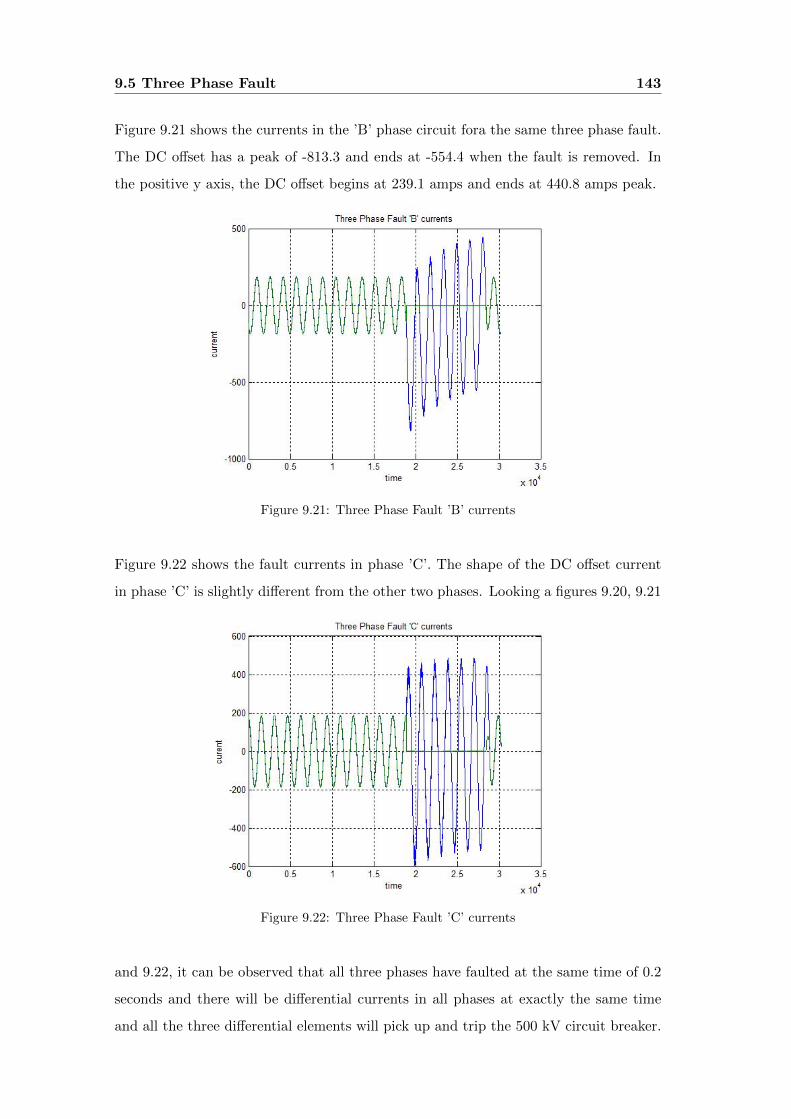
9.5 Three Phase Fault 143
Figure 9.21 shows the currents in the ’B’ phase circuit fora the same three phase fault.
The DC offset has a peak of -813.3 and ends at -554.4 when the fault is removed. In
the positive y axis, the DC offset begins at 239.1 amps and ends at 440.8 amps peak.
Figure 9.21: Three Phase Fault ’B’ currents
Figure 9.22 shows the fault currents in phase ’C’. The shape of the DC offset current
in phase ’C’ is slightly different from the other two phases. Looking a figures 9.20, 9.21
Figure 9.22: Three Phase Fault ’C’ currents
and 9.22, it can be observed that all three phases have faulted at the same time of 0.2
seconds and there will be differential currents in all phases at exactly the same time
and all the three differential elements will pick up and trip the 500 kV circuit breaker.
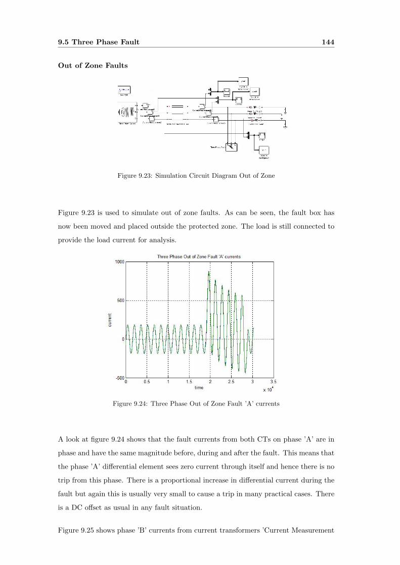
9.5 Three Phase Fault 144
Out of Zone Faults
Figure 9.23: Simulation Circuit Diagram Out of Zone
Figure 9.23 is used to simulate out of zone faults. As can be seen, the fault box has
now been moved and placed outside the protected zone. The load is still connected to
provide the load current for analysis.
Figure 9.24: Three Phase Out of Zone Fault ’A’ currents
A look at figure 9.24 shows that the fault currents from both CTs on phase ’A’ are in
phase and have the same magnitude before, during and after the fault. This means that
the phase ’A’ differential element sees zero current through itself and hence there is no
trip from this phase. There is a proportional increase in differential current during the
fault but again this is usually very small to cause a trip in many practical cases. There
is a DC offset as usual in any fault situation.
Figure 9.25 shows phase ’B’ currents from current transformers ’Current Measurement
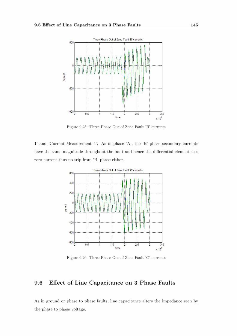
9.6 Effect of Line Capacitance on 3 Phase Faults 145
Figure 9.25: Three Phase Out of Zone Fault ’B’ currents
1’ and ’Current Measurement 4’. As in phase ’A’, the ’B’ phase secondary currents
have the same magnitude throughout the fault and hence the differential element sees
zero current thus no trip from ’B’ phase either.
Figure 9.26: Three Phase Out of Zone Fault ’C’ currents
9.6 Effect of Line Capacitance on 3 Phase Faults
As in ground or phase to phase faults, line capacitance alters the impedance seen by
the phase to phase voltage.
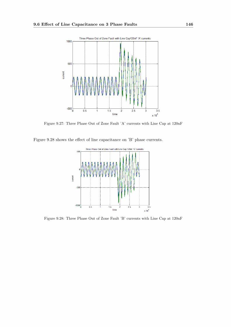
9.6 Effect of Line Capacitance on 3 Phase Faults 146
Figure 9.27: Three Phase Out of Zone Fault ’A’ currents with Line Cap at 120nF
Figure 9.28 shows the effect of line capacitance on ’B’ phase currents.
Figure 9.28: Three Phase Out of Zone Fault ’B’ currents with Line Cap at 120nF
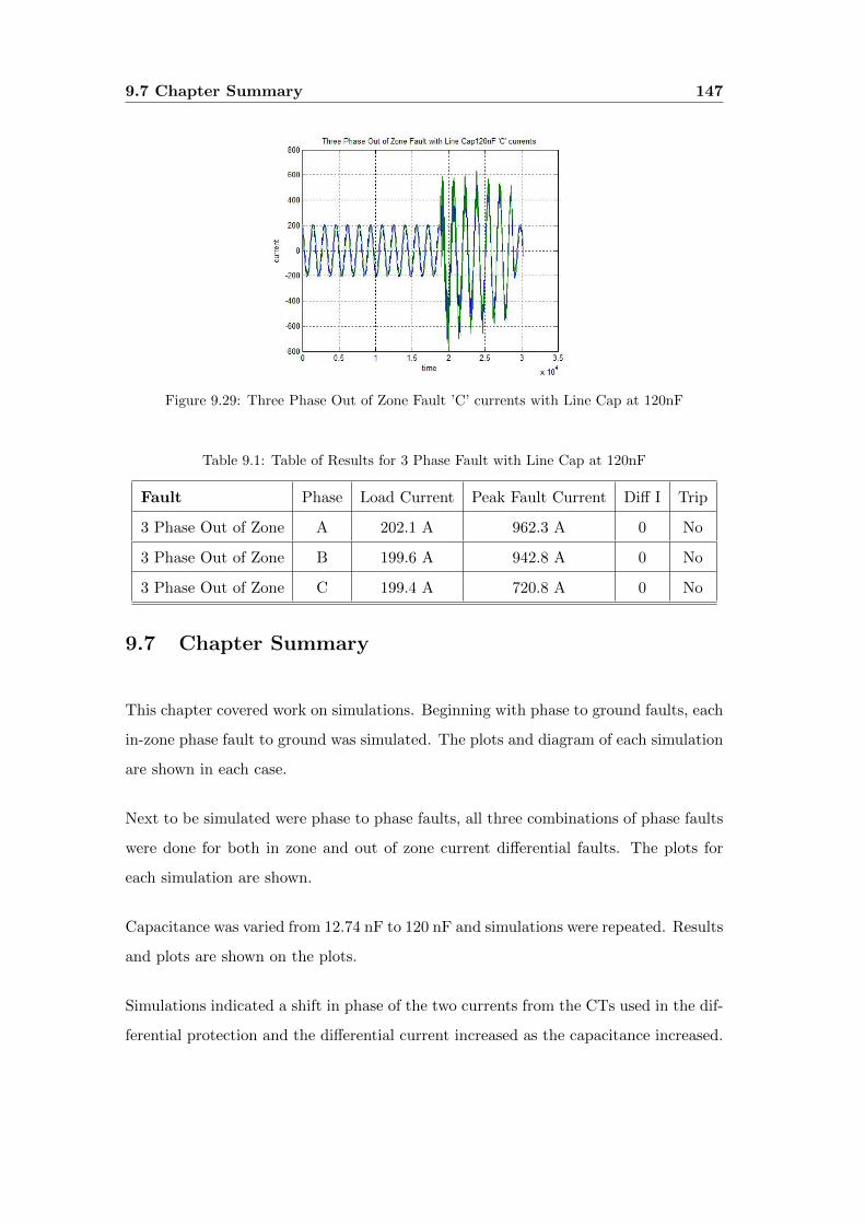
9.7 Chapter Summary 147
Figure 9.29: Three Phase Out of Zone Fault ’C’ currents with Line Cap at 120nF
Table 9.1: Table of Results for 3 Phase Fault with Line Cap at 120nF
Fault Phase Load Current Peak Fault Current Diff I Trip
3 Phase Out of Zone A 202.1 A 962.3 A 0 No
3 Phase Out of Zone B 199.6 A 942.8 A 0 No
3 Phase Out of Zone C 199.4 A 720.8 A 0 No
9.7 Chapter Summary
This chapter covered work on simulations. Beginning with phase to ground faults, each
in-zone phase fault to ground was simulated. The plots and diagram of each simulation
are shown in each case.
Next to be simulated were phase to phase faults, all three combinations of phase faults
were done for both in zone and out of zone current differential faults. The plots for
each simulation are shown.
Capacitance was varied from 12.74 nF to 120 nF and simulations were repeated. Results
and plots are shown on the plots.
Simulations indicated a shift in phase of the two currents from the CTs used in the dif-
ferential protection and the differential current increased as the capacitance increased.
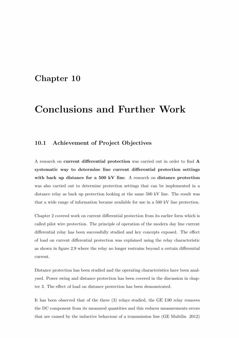
Chapter 10
Conclusions and Further Work
10.1 Achievement of Project Objectives
A research on current differential protection was carried out in order to find A
systematic way to determine line current differential protection settings
with back up distance for a 500 kV line. A research on distance protection
was also carried out to determine protection settings that can be implemented in a
distance relay as back up protection looking at the same 500 kV line. The result was
that a wide range of information became available for use in a 500 kV line protection.
Chapter 2 covered work on current differential protection from its earlier form which is
called pilot wire protection. The principle of operation of the modern day line current
differential relay has been successfully studied and key concepts exposed. The effect
of load on current differential protection was explained using the relay characteristic
as shown in figure 2.9 where the relay no longer restrains beyond a certain differential
current.
Distance protection has been studied and the operating characteristics have been anal-
ysed. Power swing and distance protection has been covered in the discussion in chap-
ter 3. The effect of load on distance protection has been demonstrated.
It has been observed that of the three (3) relays studied, the GE L90 relay removes
the DC component from its measured quantities and this reduces measurements errors
that are caused by the inductive behaviour of a transmission line (GE Multilin 2012)
10.2 Further Work 149
. An advantage of this is that there is less overshoot of the measured quantities (
typically less than 2 %) regardless of the time constant of the initial magnitude and
time constant of the DC offset. This means that the measured quantity is very nearly
its true value whenever the relay is taking measurements.
Line parameters have been investigated using the models of an overhead line. Capac-
itance measurements on a 33 kV cable were done using the Omicron CP CU1 test
equipment. It is better to calculate and also measure line parameters and compare
results before putting the line in service. This helps to get the near perfect parameters
in the relay settings.
Simulation of faults in a project is very essential in order to detect effects that may
have been overlooked during design process. Things like levels of DC offset can be
understood after enough simulations are carried out.
A systematic procedure to determine line current differential protection settings with
back up distance on a 500 kV overhead line is to follow all the steps outlined from
chapter 2 all the way to chapter 9. It should be noted that these are basic steps needed
to have the line protection working.
10.2 Further Work
Further work includes studying the effects of transients on 500 kV transmission lines
with an aim to see how protection relays respond to these transients.
Further work may involve working closely with the Aspen database to improve the
quality of relay data acquisition and storage of relays and protection information.
Further work in this project includes the involvement of the IEC 61850 standard in the
research on protection relays.
Further work involves the inclusion of auto re-close and synchro-check mechanisms as
applicable to a 500 kV overhead line.
References
ABB (2013), ‘Circuit reakers, Live Circuit Breakers, viewed 21 October 2013’, <https:
//www.abb.com./product/db003db002618/>.
Amberg, A. & Rangel, A. (2012), ‘Tutorial on Symmetrical Components,Schweitzer
EngineeringLaboratories Inc, viewed 21 August 2013’, <https://www.selinc.
com/WorkArea/DownloadAsset/aspX?=100686>.
Anderson, P. (1995), Analysis of Faulted Power Systems, 1, Wiley IEEE Press.
Arendse, P. (2010), ‘Principles of Differential Relaying, Engineers Australia, viewed 15
September 2013’, <https://www.Engineersaustralia.org.au/sites/default/
files/>.
Aspen (2013), ‘Aspen, Relay Database Software, viewed 29 July 2013’, <http://www.
aspeninc.com/aspen/>.
Bejmert, D., Rebizant, W. & Wiszniewski, W. (2011), Enhanced Differential Protection
Algorithm For Tapped Transmission Line, IEEE. http://ieeexplore.ieee.org.
ezproxy.usq.edu.au/stamp/stamp.jsp.
Calero, F. (2007), ‘Mutual Impedance In Parallel Lines Protective Relaying and
Fault Location Considerations, Schweitzer EngineeringLaboratories Inc, viewed
16 August 2013’, <https://www.selinc.com/WorkArea/DownloadAsset/aspX?
=3488>.
Dhambare, S. & Chandorkar, S. S. M. (2009), Adaptive Current Differential Protection
For Transmission Line Protection, IEEE Press. http://ieeexplore.ieee.org.
ezproxy.usq.edu.au/xpl/articleDetails.jsp.
Doble Engineering Company (2004), Doble Test Procedures, B, Doble.
REFERENCES 151
Donald, T. & Maceau, J. (2006), Asymetric operation of AC power transmission sys-
tems the key to optimizing power system reliability and economics, 1, ISBN.
Energy, G. D. (1998), ‘Digital Energy, Pilot Wire Relays, viewed 3 August 2013’,
<http://www.gedigitalenergy.com/multilin/notes/artsci/art05.pdf>.
Engineers Australia (2010), ‘Code of ethics’, http://engineersaustralia.org.au.
GE Multilin (2012), L90 differential Relay Manual, 7.0, GE.
GEC Alsthom (2011), Protective Relay Application Guide, Alsthom Grid.
GEC Measurements (1984), Micromho Relay Insruction Manual, Alsthom Grid.
Grainger, J. J. & Stevenson, W. D. (1994), Power Systems Analysis, Mcraw Hill.
Hacker, K. (1998), ‘Keith Hacker, Power System Commissioning and Practise, viewed
3 August 2013’, <http://books.googlebooks.com.au/books>.
Heading, R. A. & Hoist, S. (2012), Line Current Diferential Relay perating Under Se-
vere Transformer Saturation Conditions, IEEE. http://ieeexplore.ieee.org.
ezproxy.usq.edu.au/xpl/articleDetails.
Henville, C. (1998), ‘Digital Relay Reports Verify Power System Models’, http://
ieeexplore.ieee.org.ezproxy.usq.edu.au/stamp/stamp.jsp.
Hewitson, L. & Balakrishnan, R. (2004), Practical Power System ProtectionIDC Tech-
nologies, Practical Power System ProtectionOXFORD.
Horowitz, S. H. & Phadke, A. G. (2009), Power System Relaying, Wiley.
Ibrahim, M. A. (2012), Disturbance Analysis for Power Systems, 1, John Wiley and
Sons.
IEEE 754 Group (2004), ‘IEEE 754: Standard for Binary Floating-Point Arithmetic’,
http://grouper.ieee.org/groups/754/.
Kase, T., Kurosawa, Y. & Amo, H. (2005), ‘Charging current compensation for
distance protection’, http://ieeexplore.ieee.org.ezproxy.usq.edu.au/xpl/
articleDetails.jsp.
Kasztenny, B., Le, B. & Fischer, N. (2012), A New Multiterminal Fault Location Algo-
rithm Embeded in Line Current Differential Relays, IEEE. http://ieeexplore.
ieee.org.ezproxy.usq.edu.au/xpl/articleDetails.
REFERENCES 152
L.Bin, Wenhua, C. & Jiali, H. (2009), Special Problems in Current differential Protec-
tion Based on Bergeron Model, IEEE. http://ieeexplore.ieee.org.ezproxy.
usq.edu.au/xpl/articleDetails.
Mclaren, P. & Jayasinghe, R. P. (1997), Simulation of CTs Operating in parallel into a
differential current Protection Scheme, IEEE Press. http://ieeexplore.ieee.
org.ezproxy.usq.edu.au/xpl/articleDetails.jsp.
Megger (2004), ‘Megger, TM1600 Circuit Breaker Analysing System, viewed 20 Oc-
tober 2013’, <https://www.coast-coast.co.za/Megger/Transformertesting/
TM1600_DS_en_V02.pdf/>.
Miller, H., Burger, J. & Kasztenny, B. (2010), Modern Line Current Differential Protec-
tion Solutions, IEEE Press. http://ieeexplore.ieee.org.ezproxy.usq.edu.
au/xpl/articleDetails.jsp.
Muszaki, I. (2002), ‘Technical Guide Circuit Breake Analysis, Programma Electric AB,
viewed 15 October 2013’, <https://www.maxicont.hu/doc/hirek/GE20080402/
>.
Nise, N. S. (2007), Control Systems Engineering, 5, WILEY.
Olex Cables (2012), The 2012 Handbook, Olex Cables.
Omicron Electronics (2010), CP CU1 User Manual, Omicron.
Palm, W. (2011), Introduction to Matlab for Engineers, 3, McGraw Hill.
Pardo, J., Elmore, J. & Doung, V. (2012), ‘500kV IPT Breaker Failure Protection,
An application of dual timer Scheme for Short Critical clearing Time’, <https:
//www.ieeexplore.ieee.org.ezproxy.usq.edu.au/>.
Pas, H. P. (1993), Analog and Digital Communications, Schaum’s Outline Series,
McGraw-Hill.
Prorgramma Products (2009), ‘TM1600 MA61, Programma Products, viewed 20 Oc-
tober 2013’, <https://www.lecom.com.cn/Upfiles/200941354731.pdf/>.
Rincorn, C. & Perez, J. (2012), Calculating Loadability Limits of Distance Relays,
Protective Engineers IEEE. http://ieeexplore.ieee.org.ezproxy.usq.edu.
au/xpl/articleDetails.jsp.
REFERENCES 153
Schweitzer Engineering Laboratories (2003), SEL 3111L Manual, SEL.
Schweppes, C. (2002), ‘The importance of ethics in bussiness’, http://www.
bussinesscasestudues.co.
Shateri, H. & Jamali, S. (2008), ‘Measured impedance at relaying point consider-
ing line capacitance’, http://ieeexplore.ieee.org.ezproxy.usq.edu.au/xpl/
articleDetails.jsp.
Siemens (2011), 7SD5 RELAY Manual, Siemens.
Siemens (2012), ‘Siemens, 7PG21 Solkor R RF Relay Manual, viewed 29 July 2013’,
<http://www.energy.siemens.com/ecc_pool/REYROLLE_Protect>.
Sondhi, M. M., Morgan, D. R. & Hall, J. L. (1995), ‘Stereophonic Acoustic Echo
Cancellation – An Overview of the Fundamental Problem’, IEEE Signal Processing
Letters 2(8), 148–151.
SP Ausnet (2007), Contractor Health Safety and Environmental Rules, 10, SP AusNet.
Survevors Board Queensland (2010), ‘Code of ethics’, http://sbq.com.au/public/
more-information/code-of-practice.
TYAGI, A. K. (2012), Matlab and Simulink for Engineers, OXFORD.
Tziouvaras, D., Art, B. & Bill, L. (2005), ‘Power Swing and Out Of Step Considerations
on Transmission Lines, IEEE PSRC WG 6, viewed 2 August 2013’, <http://www.
pes-psrc.org/Reports/archive/Apublications>.
University of Southern Queensland (2013), Power Systems Protection Study Book, 1,
USQ.
Victorian Electricity Supply Industry (2006), The Green Book Code of Practise on
Electrical Safety for the Distribution bussiness in Victoria, VESI.
Voloh, I. & Johnson, R. (2005), ‘Applying digital line current differential relays over pi-
lot wires’, http://ieeexplore.ieee.org.ezproxy.usq.edu.au/stamp/stamp.
Wang, J. & etal (2000), Tests On The First 500 kV Compact Transmission Line
in China, IEEE. http://ieeexplore.ieee.org.ezproxy.usq.edu.au/xpl/
articleDetails.jsp.

REFERENCES 154
Xue, Y., Finney, D. & Le, B. (2012), ‘Charging Current in Long Lines and High Voltage
Cables, American Electric Power ,Schweitzer EngineeringLaboratories Inc, viewed
14 August 2013’, <https://www.selinc.com/WorkArea/DownloadAsset/aspX?
=101004>.
Zeek, J., Adamiak, M., Voloh, I. & Kastenny, B. (n.d.), ‘Application of Current Dif-
ferential Protection to Tapped Transmission Lines, General Electric , viewed 15
September 2013’, <https://www.store.geDigitalenergy.com/faq/documents/
L90/GER-3978>.

Appendix A
Project Specification
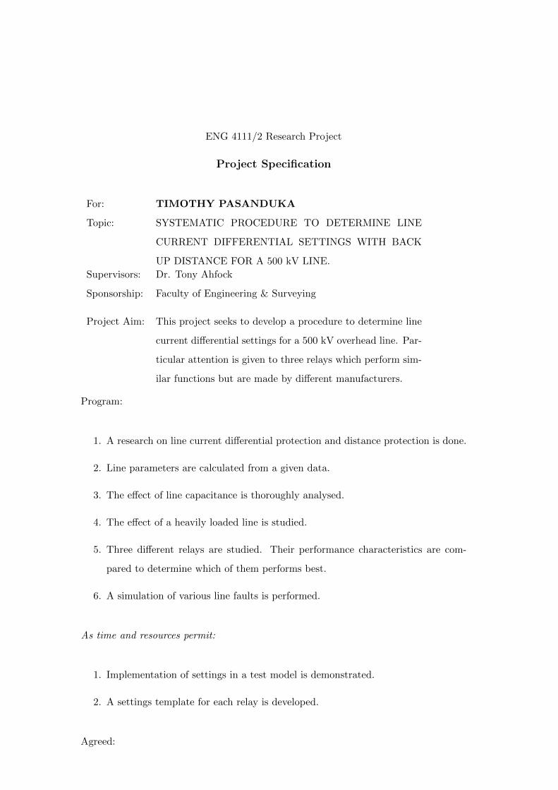
ENG 4111/2 Research Project
Project Specification
For: TIMOTHY PASANDUKA
Topic: SYSTEMATIC PROCEDURE TO DETERMINE LINE
CURRENT DIFFERENTIAL SETTINGS WITH BACK
UP DISTANCE FOR A 500 kV LINE.
Supervisors: Dr. Tony Ahfock
Sponsorship: Faculty of Engineering & Surveying
Project Aim: This project seeks to develop a procedure to determine line
current differential settings for a 500 kV overhead line. Par-
ticular attention is given to three relays which perform sim-
ilar functions but are made by different manufacturers.
Program:
1. A research on line current differential protection and distance protection is done.
2. Line parameters are calculated from a given data.
3. The effect of line capacitance is thoroughly analysed.
4. The effect of a heavily loaded line is studied.
5. Three different relays are studied. Their performance characteristics are com-
pared to determine which of them performs best.
6. A simulation of various line faults is performed.
As time and resources permit:
1. Implementation of settings in a test model is demonstrated.
2. A settings template for each relay is developed.
Agreed:

157
Student Name: Timothy Pasanduka
Date: March 2013
Supervisor Name: Tony Ahfock
Date: March 2013
Examiner/Co-Examiner:
Date:

Appendix B
Some Supporting Information
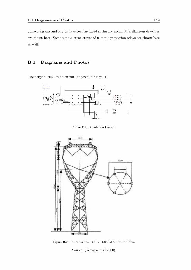
B.1 Diagrams and Photos 159
Some diagrams and photos have been included in this appendix. Miscellaneous drawings
are shown here. Some time current curves of numeric protection relays are shown here
as well.
B.1 Diagrams and Photos
The original simulation circuit is shown in figure B.1
Figure B.1: Simulation Circuit.
Figure B.2: Tower for the 500 kV, 1320 MW line in China
Source: (Wang & etal 2000)
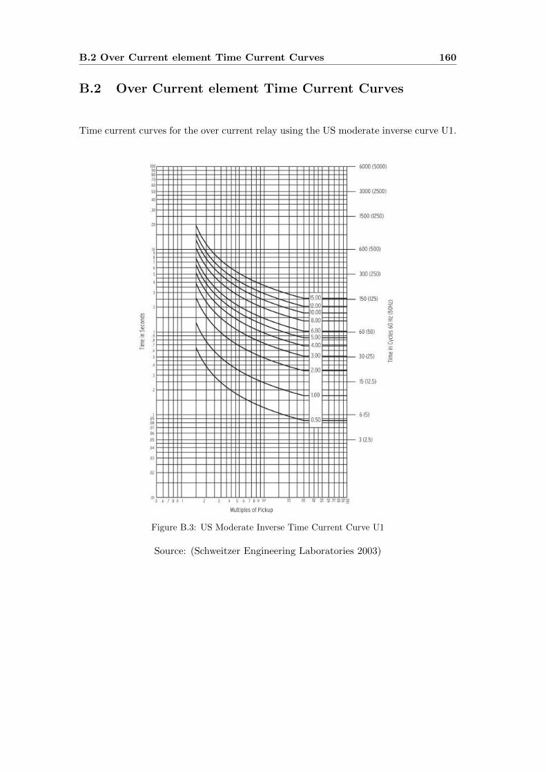
B.2 Over Current element Time Current Curves 160
B.2 Over Current element Time Current Curves
Time current curves for the over current relay using the US moderate inverse curve U1.
Figure B.3: US Moderate Inverse Time Current Curve U1
Source: (Schweitzer Engineering Laboratories 2003)
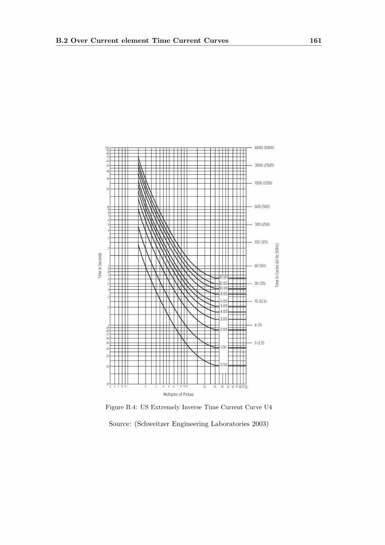
B.2 Over Current element Time Current Curves 161
Figure B.4: US Extremely Inverse Time Current Curve U4
Source: (Schweitzer Engineering Laboratories 2003)

Appendix C
Project Timeline
The chart below shows the gantt chart for the project. The chart begins with Prelimi-
nary Work activity and ends with activity Submission.
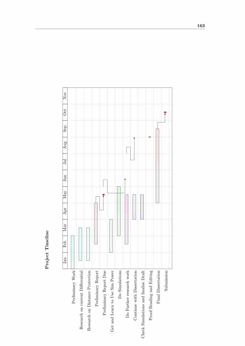
163
Pro
ject
Tim
eline
Jan
Feb
Mar
Ap
rM
ayJu
nJu
lA
ug
Sep
Oct
Nov
Pre
lim
inary
Work
Res
earc
hon
curr
ent
Diff
eren
tial
Res
earc
hon
Dis
tan
ceP
rote
ctio
n
Pre
lim
inar
yR
epor
t
Pre
lim
inar
yR
eport
Du
e
Get
an
dL
earn
toU
seS
imP
ower
Do
Sim
ula
tion
s
Do
Fu
rth
erre
searc
hw
ork
Conti
nu
ew
ith
Dis
sert
atio
n
Ch
eck
Sim
ula
tion
san
dfi
nal
ise
Dra
ft
Pro
ofR
ead
ing
and
Ed
itin
g
Fin
alD
isse
rtat
ion
Su
bm
issi
on